STRATEGIC DECISION-MAKING OF FLEXIBLE

INVESTMENTS UNDER UNCERTAINTIES IN LONG-TERM

ELECTRICITY MARKETS

DANIEL ALBERTO RIOS FESTNER

Thesis submitted to the Polytechnic Faculty of the National University of Asunción,

in partial fulfillments of the requirements for the degree of Master of Science in

Electrical Engineering

SAN LORENZO – PARAGUAY

October – 2017

STRATEGIC DECISION-MAKING OF FLEXIBLE

INVESTMENTS UNDER UNCERTAINTIES IN LONG-TERM

ELECTRICITY MARKETS

DANIEL ALBERTO RIOS FESTNER

Advisor: Prof. Dr. GERARDO ALEJANDRO BLANCO BOGADO

Thesis submitted to the Polytechnic Faculty of the National University of Asunción,

in partial fulfillments of the requirements for the degree of Master of Science in

Electrical Engineering

SAN LORENZO – PARAGUAY

October – 2017

Ríos Festner, Daniel Alberto.

Strategic Decision-Making of Flexible Investments under Uncertainties in

Long-Term Electricity Markets / Daniel Alberto Ríos Festner - - San Lorenzo, 2017.

68 p.: il.

Tesis (Maestría en Ciencias de la Ingeniería Eléctrica - - Facultad Politécnica

de la Universidad Nacional de Asunción, 2017).

Bibliografía y Apéndice

1. Generation 2. Real Options 3. Stochastic 4. Strategic Flexibility

5. System Dynamics. 6. Simulation I. Titulo.

CDD 333.793 23

To Julia Carmen, Natalia, Fernando and Harald, an unusual but compelling group

A Julia Carmen, Natalia, Fernando y Harald, un grupo inusual pero convincente

Acknowledgments

I have no words to thank all the people who have accompanied me during this time. However, I think it is fair enough to recognize the following:

First, I wish to express my sincerest gratitude to my advisor, Prof. Dr. Gerardo Blanco, for giving me the opportunity to write this thesis at the Research Group in Energy Systems (GISE-FPUNA). During the last two years, I have deeply appreciated his insightful guidance and unrestrictive support, especially, in the most difficult of times.

I am greatly indebted to Prof. Dr. Fernando Olsina, as well as to Prof. Dr. Francisco Garcés and Prof. Dr. Rolando Pringles, for accepting me at the Institute of Electrical Engineering (IEE), National University of San Juan (UNSJ), Argentina. My visit to the IEE has been certainly rewarding, and it has far excelled any previous expectation.

I would like to thank Prof. Dr. Victorio Oxilia, on behalf of the entire team at GISE-FPUNA, for giving the example in creating the best work environment one could wish for on a daily basis. I wish to express my gratitude particularly to Diana and Gabriel, who made me feel at home when I visited San Juan, Argentina.

I would not be writing these lines without the love and support of my family: my parents, Ilse and Alberto, and my siblings Claudia and Hugo. Likewise, I thank God for the life of my four grandparents. Last, but not least, I am very grateful to my fiance Cristina for her love, her patience, and for sharing dreams and projects together.

I would like to especially remark the financial support of the National Council of Science and Technology from Paraguay (CONACYT) in the development of this research work.

GRACIAS TOTALES!

Daniel, October 26th, 2017

Agradecimientos

No tengo palabras para agradecer a todas las personas que me han acompañado durante esta etapa. Sin embargo, creo justo reconocer lo siguiente:

Primero, deseo expresar mi sincera gratitud a mi tutor, Prof. Dr. Gerardo Blanco, por darme la oportunidad de trabajar en el Grupo de Investigación en Sistemas Energéticos (GISE-FPUNA). Durante los últimos dos años, he tenido un profundo aprecio por su lúcida dirección e irrestricto apoyo, sobre todo, en los momentos de mayor dificultad.

Asimismo, agradezco al Prof. Dr. Fernando Olsina, así como al Prof. Dr. Francisco Garcés y al Prof. Dr. Rolando Pringles, por aceptarme en el Instituto de Ingeniería Eléctrica (IEE), Universidad Nacional de San Juan (UNSJ), Argentina. Mi experiencia en el IEE ha sido gratificante, y ha superado con creces cualquier expectativa previa.

Me gustaría agradecer al Prof. Dr. Victorio Oxilia, en representación de todo el equipo del GISE-FPUNA, por dar el ejemplo para crear diariamente el mejor ambiente de trabajo que uno puede desear. Quisiera agradecer particularmente a Diana y Gabriel, quienes me hicieron sentir como en casa cuando visité San Juan, Argentina.

No estaría escribiendo estas líneas sin el amor y apoyo de mi familia: mis padres, Ilse y Alberto, y mis hermanos Claudia y Hugo. También agradezco a Dios por la vida de mis cuatro abuelos. Por último, pero no menos importante, estoy muy agradecido con mi novia Cristina por su amor, su paciencia, y por compartir sueños y proyectos juntos.

Quisiera destacar especialmente además el apoyo financiero del Consejo Nacional de Ciencia y Tecnología de Paraguay (CONACYT) para el desarrollo de este trabajo.

¡Gracias totales!

Daniel, 26 de octubre de 2017

STRATEGIC DECISION-MAKING OF FLEXIBLE

INVESTMENTS UNDER UNCERTAINTIES IN LONG-TERM

ELECTRICITY MARKETS

Author: DANIEL ALBERTO RIOS FESTNER

Advisor: Prof. Dr. GERARDO ALEJANDRO BLANCO BOGADO

SUMMARY

In liberalized electricity markets, the investment postponement option is deemed to be decisive for understanding the addition of new generating capacity. Basically, it refers to the investors’ chance to postpone projects for a period while waiting for the arrival of new and better information about the market evolution. When such development involves major uncertainties, the generation business becomes riskier, and the investors’ “wait-and-see” behavior might limit the timely addition of new generation capacity. The literature provides solid empirical evidence about the occurrence of construction cycles in the deregulated electricity industry. However, the strategic flexibility inherent to defer investments in power plants has not been yet rigorously incorporated as an explicit input for investment signals in the revised long-term market models. Therefore, this paper proposes a new methodology to assess the long-term development of liberalized power markets based on a more realistic approach for valuing generation investments. The proposal is based on a stochastic dynamic market model, built upon a System Dynamics simulation approach. The model considers that the addition of new generation capacity is driven by the economic value of the strategic flexibility associated to defer investments under uncertainties. The value of the postponement option is quantified in monetary terms by means of Real Options analysis. Simulations explicitly confirm the cyclical behavior of the energy-only market in the long-run, as suggested by the empirical evidence found in the literature. Furthermore, the proposed method is used to test three regulatory schemes, implemented in order to dampen the arising construction cycles. Results show that, for ensuring the supply security in markets under huge uncertainties, investors would need complementary capacity incentives in order to deploy power generation investments in timely manner.

Key words: Generation, Real Options, Stochastic Simulation, Strategic Flexibility, System Dynamics.

MODELO DE TOMA DE DECISIONES BAJO

INCERTIDUMBRE EN MERCADOS ELÉCTRICOS A LARGO

PLAZO

Autor: DANIEL ALBERTO RIOS FESTNER

Orientador: Prof. Dr. GERARDO ALEJANDRO BLANCO BOGADO

RESUMEN

En mercados de electricidad liberalizados, la opción de posponer inversiones se considera decisiva para entender la incorporación de nueva capacidad de generación. Básicamente, dicha opción se refiere a la posibilidad de que los inversores aplacen proyectos durante cierto tiempo mientras esperan la llegada de nueva y mejor información acerca de la evolución del mercado. Cuando tal desarrollo involucra grandes incertidumbres, el negocio de generación se vuelve más riesgoso, y el comporamiento de “esperar y ver” de los inversores puede limitar la adición oportuna de nueva capacidad de generación. La literatura proporciona evidencia empírica sólida sobre la ocurrencia de ciclos de construcción en la industria desregulada de electricidad. No obstante, la flexibilidad estratégica inherente a posponer inversiones en centrales eléctricas aún no ha sido rigurosamente incorporada como una entrada explícita de las señales de inversión en los modelos de mercado de largo plazo revisados. Por lo tanto, este trabajo propone una nueva metodología con el objetivo de evaluar el desarrollo a largo plazo de los mercados eléctricos liberalizados en base a un enfoque más realista para valorar inversiones en generación. La propuesta se basa en un modelo de mercado dinámico y estocástico, elaborado mediante el enfoque de simulación Dinámica de Sistemas. El modelo considera que la adición de nueva capacidad de generación está impulsada por el valor económico de la flexibilidad estratégica asociada a diferir inversiones bajo incertidumbre. El valor de la opción de posponer se cuantifica en términos monetarios mediante el análisis de las Opciones Reales. Las simulaciones confirman de forma explícita el comportamiento cíclico del mercado de energía a largo plazo, como lo sugiere la evidencia empírica encontrada en la literatura. Además, el método propuesto se utiliza para estudiar tres medidas regulatorias, aplicadas con el objetivo de amortiguar los ciclos resultantes. Los resultados muestran que, para asegurar la seguridad del suministro en mercados bajo grandes incertidumbres, los inversionistas necesitarían incentivos de capacidad complementarios para desplegar inversiones en centrales de generación de manera oportuna.

Palabras claves: Dinámica de Sistemas, Flexibilidad Estratégica, Generación, Opciones Reales, Simulación Estocástica.

CONTENTS

Page

I INTRODUCTION ................................................................................................... 1

II STATE-OF-THE-ART REVIEW ........................................................................ 6

Chapter 1 Power investment decision-making under uncertainty................... 6

1.1 Power investments in liberalized electricity markets ............................. 6

1.2 Current development of long-term electricity market models ............... 7

1.3 Valuing generation investments under uncertainties ........................... 10

III METHODOLOGY ............................................................................................. 13

Chapter 2 Scope of the thesis ............................................................................. 13

Chapter 3 Valuing flexible investments with Real Options ............................ 16

3.1 Traditional investment valuation approach .......................................... 16

3.2 Valuing investments under uncertainty and risk .................................. 17

3.3 Option analysis applied to power generation investments ................... 19

3.4 Real Options valuation methods .......................................................... 22

Chapter 4 Decision-making of flexible investments under uncertainties within

long-term electricity market models ............................................... 25

4.1 Model overview ................................................................................... 25

4.2 Simulation of the long-term power market dynamics .......................... 26

4.3 Simulation of investors’ expectation formation upon profitability ...... 30

4.4 Simulation of investors’ decision-making under uncertainties ............ 36

IV RESULTS & DISCUSSION .............................................................................. 41

Chapter 5 Simulation analysis ........................................................................... 41

5.1 System data and initial conditions ....................................................... 41

5.2 Base case simulation ............................................................................ 43

5.3 Sensitivity analysis on exogenous market variables ............................ 44

5.4 Policy implications ............................................................................... 48

5.5 Sensitivity analysis on Real Options parameters ................................. 53

V CONCLUSIONS .................................................................................................. 56

BIBLIOGRAPHICAL REFERENCES ................................................................. 58

APPENDIX ............................................................................................................... 63

A1 Modeling expectations upon profitability in the Capacity Market ...... 63

A2 Modeling expectations upon profitability with Capacity Payments .... 65

A3 Modeling the performance metrics of the capacity adequacy .............. 66

PUBLICATIONS ..................................................................................................... 67

ABOUT THE AUTHOR ......................................................................................... 68

LIST OF FIGURES

Page

Figure 1: Causal Loop Diagram of the long-term dynamics of electricity markets

according to the literature. ........................................................................ 9

Figure 2: Causal Loop Diagram of the long-term dynamics of electricity markets

with the proposed decision-making framework. .................................... 26

Figure 3: Investment multiplier as a function of the profitability index. ............... 29

Figure 4: Simulation of current (at �) and expected (at ��) demand growth at any

time. ........................................................................................................ 34

Figure 5: Example of the schematic definition of a Price Duration Curve (PDC). 34

Figure 6: Investment decision regions in the Exercise-Continuation Value plane. 40

Figure 7: Simulation of evolution of installed capacity and reserve margin. ........ 45

Figure 8: Simulation of evolution of market price. ............................................... 45

Figure 9: Simulation of evolution of reserve margin with different Load Growth

Rates (LGR). .......................................................................................... 47

Figure 10: Simulation of evolution of reserve margin with different volatilities of the

LGR. ....................................................................................................... 47

Figure 11: Simulation of evolution of reserve margin with different volatilities of fuel

prices growth rates. ................................................................................ 49

Figure 12: Simulation of evolution of reserve margin with the adoption of regulatory

schemes. ................................................................................................. 51

Figure 13: Simulation of evolution of market price with the adoption of regulatory

schemes. ................................................................................................. 51

Figure 14: Performance metrics of capacity adequacy with the adoption of regulatory

schemes. ................................................................................................. 52

Figure 15: Simulation of evolution of reserve margin with different maturities for the

postponement option. ............................................................................. 54

Figure 16: Simulation of evolution of reserve margin with different risk-free discount

rates. ....................................................................................................... 55

LIST OF TABLES

Page

Table 1: Input data for the generation test system. ............................................... 42

Table 2: Parameters of the logistic function for the multiplier of the investment rate

for each technology. ............................................................................... 42

Table 3: Parameters to characterize the stochastic growth rates of maximum and

minimum demand (��), total installed capacity (��), fuel price of hard-

coal (���,����) and fuel price of natural gas (���,���). ........................... 42

Table 4: Performance metrics of capacity adequacy with the adoption of regulatory

schemes. ................................................................................................. 52

Table 5: Input data for the scenario simulation with different maturities for the

postponement option. ............................................................................. 54

LIST OF ACRONYMS & ABBREVIATIONS

AUE Annual-average Unitary Expenditure.

CCGT Combined Cycle Gas Turbine.

CLD Causal Loop Diagram.

CT Construction Time

CVaR Conditional Value at Risk.

DDE Delay Differential Equation.

DPE Dynamic Programming based on the Expected value.

DT Decision Time

EUR Euro.

FACTS Flexible Alternative Current Transmission System.

FO Financial Options

GAST Gas Turbine.

GW Gigawatt.

HACO Hard Coal.

IEA International Energy Agency.

IRR Internal Revenuel Rate.

LDC Load Duration Curve.

LGR Load Growth Rate.

LOLP Lost of Load Probability.

MW Megawatt.

MWh Megawatt-hour.

NPV Net Present Value.

PDC Price Duration Curve.

PDE Partial Differential Equation.

PI Profitability Index.

RO Real Options.

RSME Root Square Mean Error.

SD System Dynamics.

TRM Target Reserve Margin.

VaR Value at Risk.

VOLL Value of Lost Load.

WACC Weighted Average Cost of Capital.

I INTRODUCTION

In the last three decades, the evolution towards liberalization of electricity markets has

pursued the main objective of improving the economic efficiency of the supply side

(IEA, 2003). The deregulation has been founded on strictly market mechanisms, which

has led to the unbundling of the industry and the introduction of competition, mainly,

in the generation segment. Despite many positive outcomes, the cumulated experience

after the first stage of reforms has also raised concerns regarding the market attributes

that needed to ensure the capacity adequacy (e.g. Rudnick et al., 2005; Arango et al.,

2006; Joskow, 2006). At first, this seems counterintuitive, since the theory of spot

pricing, upon which the deregulation is based, ideally provides sufficient investment

incentives in the long run (Caramanis, 1982). However, it has been reported repeatedly

since the beginning of the 1990s (e.g. Bunn and Larsen, 1992; Bunn and Larsen, 1994)

that the liberalized power industry is instead prone to suffer construction cycles1.

Many efforts have been put in order to understand the origins of this situation. One of

the most accepted explanations poses that the theoretical models that have supported

the deregulation rely on assumptions absent in real power markets, such as perfect

competition, risk neutrality and full rational behavior of market participants. Indeed,

actual markets are likely to deviate from ideal conditions, exhibiting imperfections

such as information asymmetry, risk aversion, herding behavior and bounded rational

expectations. Moreover, investors in power plants have the possibility of behaving

strategically in order to collect extraordinary profits, being prone to exercise market

1 This term refers to the fluctuating development that the capacity is perceived to have exhibited after being deregulated, due to the sequential episodes of over and under-investment.

2

power or to be unresponsive to straight market signals. In that sense, integrating the

logic behind the strategic decision-making of new generating capacity has become

vital when assessing the long-term market development.

A comprehensive literature compilation that suggests the appearance of cycles in the

construction of investor-owned power plants has been proposed by Arango and Larsen

(2011). Such work presents empirical evidence gathered from over 20 years of reforms

in electriciy markets, with England and Wales, and Chile giving the most exemplary

cases. The article explains that the unstable market behavior leads to periods with low

reserve margins, mainly affecting the demand side in terms of high prices and recurrent

shortages. However, in times of excess of capacity, generation companies are likely to

endure substantial economic losses, and potential bankruptcy. Therefore, the cyclical

investment pattern is deemed to pose major concerns for policymakers when assessing

the long-run development of the market, since it ultimately affects the security of

supply (Roques, 2008).

Despite the abundance of empirical evidence, the literature still lacks a rigorous

mathematical framework for describing, in theoretical terms, the cyclical behavior of

liberalized power markets. Nevertheless, it is worth to acknowledge that significant

modeling efforts have been done for assessing the long-run behavior of the industry

(Ventosa et al., 2005). Several works have focused on including some behavioral

aspects of investors in long-term power market models. Notwithstanding, the methods

proposed up to this day are based on simplifying the risk-averse profile that defines

the investors’ response, by adjusting their expectations upon profitability according to

predefined patterns. Thus, it is deemed that the literature can be enhanced by including

the behavioral nature driving the adequacy of capacity in current power markets.

In that context, this research work pursues the following general objective:

Formulate mathematically the investment decision-making process within liberalized

electricity markets with the consideration of the flexibility of postponing new power

plants under uncertainty.

3

Likewise, the following specific objectives are aimed to be accomplish:

Integrate a valuation framework of flexible investments with a long-term dynamic

model of a liberalized electricity market.

Provide a rigorous mathematical formulation for explaining the occurrence of

construction cycles in liberalized electricity markets.

Analyze aditional capacity remuneration mechanisms for dampening the arising

business cycles in order to improve the long-term market stability.

As mentioned previously, the liberalization of electricity markets has changed the

scope of decision-making in new generating capacity. Under this paradigm, multiple

self-oriented companies aim at maximizing their own profits, defining a market

behavior that is dynamic in nature. Therefore, investors need to develop sufficient

certainty about the recovery of vast capital costs before undertaking new power plants.

In fact, it has been perceived that investors are prone to postpone investments while

waiting for the arrival of new and better information about the uncertain market

evolution. In that context, firms might constrain the entrance of new generating

capacity even during upward movements of the market, because they expect more

profitable conditions in the future. The investment execution will become attractive

eventually but then, an excess of optimism might lead to a situation of over-capacity,

where more power plants than needed are undertaken.

By following this reasoning, this research work hypothesizes that the cyclical behavior

of the deregulated electricity industry originate because of the inclination of companies

for postponing new power plants under uncertainties, jointly with the delay due to the

construction time. In order to prove this hypothesis, a novel framework for describing

the decision-making of generation investments is integrated with a power industry

model, aiming to assess its long-term development. The proposed approach is suitable

for capturing the strategic behavior of investors when making investment decisions,

mainly because it includes the possibility of postponing new power plants in the

definition of an optimal investment policy.

4

Taking into consideration the unpredictable effects of construction cycles, the long-

term development of liberalized electricity markets involves a key topic of study. Thus,

it is supposed that the lack of a mathematical explanation for the origins of such

fluctuating behavior prevents market stakeholders of conducting more refined

assessments of their activities.

More specifically, this situation concerns power firms considering investments in

generating capacity. According to the rules of the deregulated industry, these firms are

set to take advantage of any market context in order to maximize their own profits. In

that sense, opportunities for seizing market upward movements, or to cut losses during

unfavorable situations, are of a great value. Hence, the formal description of factors

driving the long-term market behavior implies the potential of significant benefits for

generating firms.

Appropriate models are equally crucial for regulatory authorities. The availability of a

rigorous market modeling framework is essential to simulate the suitability of different

designs and policies intended to ensure the market stability and the security of supply

in the long term. During the last years, this issue has been at the center of interest, since

many countries have started to implement alternative mechanisms for remunerating

the capacity, besides the energy-only market. This has aimed to promote a stable pace

for the capacity expansion by reducing risks associated to the investment cycles in

power generation.

The chapters at the thesis are organized as follows. Chapter 1 includes a state-of-the-

art review about the subject under study. In accordance with such review, the scope of

the research work is delimited specifically in Chapter 2. Then, in Chapter 3, the Real

Options (RO) method for valuing flexible investments in the liberalized electricity

industry is presented. Chapter 4 contains the mathematical formulation of the long-

term dynamic market model adopted for this study; the description of uncertainties

driving the market development; the investor’s formation of expectations upon

profitability, and the proposed decision-making framework based on RO analysis.

Finally, results and key findings are analyzed in Chapter 5, including the base case

5

simulations; sensitivity analyzes to test the robustness of the proposed framework; and

the implementation of three regulatory schemes aiming to dampen the arising business

cycles.

II STATE-OF-THE-ART REVIEW

Chapter 1

Power investment decision-making under uncertainty

1.1 Power investments in liberalized electricity markets

Two factors can be isolated in order to gain insights about the occurrence of

construction cycles in the deregulated electricity industry. First, the decision to expand

the system has decentralized to depend on multiple self-oriented, autonomous firms,

who attempt to maximize solely their financial profits while managing risks. This

defines a market behavior that is dynamic in nature, since it is determined by the

actions of individual participants (de Vries and Heijnen, 2008). The second and most

important factor indicates that the generation activity has become exposed to several

risks, unforeseen in the former regulated industry. Such risks result from the

internalization of numerous uncertainties that drive the development of the actual

industry in the long run (IEA, 2003; Arango and Larsen, 2011).

The effects of these factors are multiplied by intrinsic features of generation

investments. Some of these particularities are listed in the following (Olsina et al.,

2006):

Capital-intensive: Investments in generating capacity involve large financial costs.

In fact, power plants normally account for most of the capital expenditures inherent

to the electricity industry.

7

One-step: A significant proportion of the total financial costs must be committed

before the power plant becomes operative.

Long amortization periods: Several years are agreed so the incurred outlay can be

paid off.

Irreversibility: Power plants are unlikely to serve for other purposes if market

conditions turn the generation activity unprofitable. Therefore, investments in

generating capacity are considered sunk costs.

Given the characteristics of the competitive generation business, investors tend to be

risk-averse when making investment decisions (Vázquez et al., 2002). Generally, this

rationale suggests that new generating units would be ordered only when large

revenues are expected, and conversely decisions would be delayed if the estimated

rents are insufficient. Hence, opportunities for investing in the generation sector are

no longer of the now-or-never type since there is the possibility of waiting for future

market conditions to be, at least partially, clarified. This opportunity incorporates one

major attribute to the deregulated generation investments, termed the postponement

option (Olsina et al., 2006). It explains the investors’ willingness to consider the

flexibility of deferring new generation investment projects when facing uncertainties

driving the evolution of key market variables (Blanco and Olsina, 2011).

1.2 Current development of long-term electricity market models

In the context of the present study, the model of a liberalized electricity market is used

for gaining insights about the long-term evolution of its structural parameters, namely

the installed capacity. Since the addition of new power plants now involves multiple,

self-oriented companies, it is essential that the model incorporates the logic behind

their autonomous decision-making.

Several modeling approaches are suitable for describing the long-run behavior of the

deregulated industry, from a financial point of view (Sterman, 1991). In particular, it

has been found that simulation models are appropriate for capturing actual behavioral

8

features of investors in liberalized markets, such as bounded rationality, learning

abilities, imperfect foresight, etc. (Ventosa et al., 2005). In that context, System

Dynamics (SD) is a modeling approach with a vast literature body regarding the

development of simulation models of complex systems (Baum et al., 2015). The SD-

based approach focuses on identifying the feedback structure of a system, at a

macroscopic level, and the logical interrelationships among its components. Then, it

aims to deliver a dynamic response in the long term by solving the governing non-

linear differential equations. A well-founded background on this subject is the work

by Sterman (2000).

Generally, dynamic models are well-known for suggesting a volatile long-term

behavior of the deregulated power sector. The situation is explained due to the

inherently unstable interaction between the power exchange and the profitability

expectation of investors. In order to gain insights about this complex interaction, SD

provides a tool known as the Causal Loop Diagram (CLD), which helps in giving an

initial perspective about the feedback structure of the system under analysis. Such

perspective eventually allows to formulate the differential equations that must describe

rigorously the long-term system dynamics.

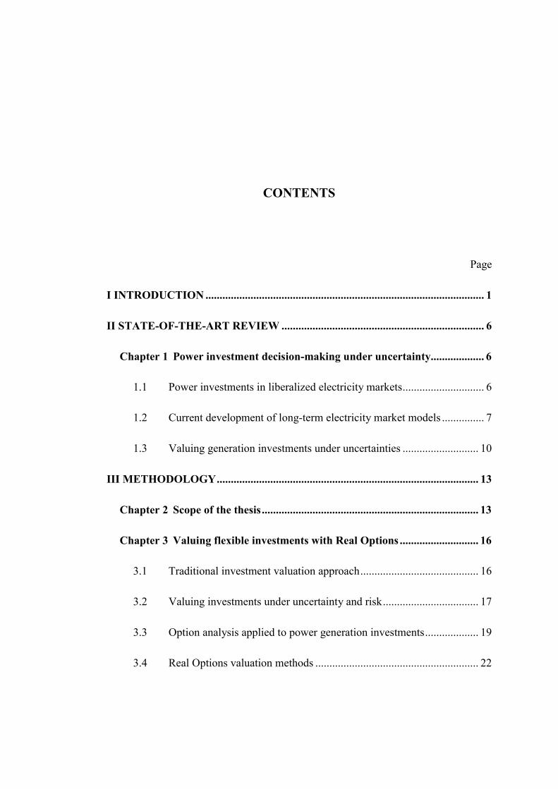
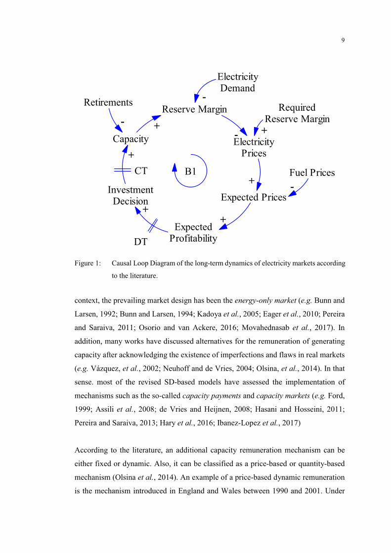
The literature contains an example of the feedback structure that formalizes the process

of capacity expansion in this study context by means of a CLD (Olsina et al., 2006).

Such diagram is included in Figure 1. Unlike in the centralized paradigm, here a delay

representing the investors’ decision-making under uncertainties is one of the factors

preventing the timely adequacy of the installed capacity. This delay represents the

Decision Time (DT) necessary for investors to develop enough certainty about the

recovery of capital costs. Since investments in power plants are no longer of the now-

or-never type, investors are then likely to wait for the arrival of new and better

information before undertaking new investment projects.

With the advent of deregulation of the power industry, the decision-making of new

generation investments has come to depend upon profitability expectations. In that

9

Capacity

InvestmentDecision

ExpectedProfitability

Retirements

+

-

+

Reserve Margin

ElectricityDemand

ElectricityPrices

Expected Prices

+

-

-

+

+

Fuel Prices

-

B1CT

RequiredReserve Margin

+

DT

Figure 1: Causal Loop Diagram of the long-term dynamics of electricity markets according

to the literature.

context, the prevailing market design has been the energy-only market (e.g. Bunn and

Larsen, 1992; Bunn and Larsen, 1994; Kadoya et al., 2005; Eager et al., 2010; Pereira

and Saraiva, 2011; Osorio and van Ackere, 2016; Movahednasab et al., 2017). In

addition, many works have discussed alternatives for the remuneration of generating

capacity after acknowledging the existence of imperfections and flaws in real markets

(e.g. Vázquez, et al., 2002; Neuhoff and de Vries, 2004; Olsina, et al., 2014). In that

sense. most of the revised SD-based models have assessed the implementation of

mechanisms such as the so-called capacity payments and capacity markets (e.g. Ford,

1999; Assili et al., 2008; de Vries and Heijnen, 2008; Hasani and Hosseini, 2011;

Pereira and Saraiva, 2013; Hary et al., 2016; Ibanez-Lopez et al., 2017)

According to the literature, an additional capacity remuneration mechanism can be

either fixed or dynamic. Also, it can be classified as a price-based or quantity-based

mechanism (Olsina et al., 2014). An example of a price-based dynamic remuneration

is the mechanism introduced in England and Wales between 1990 and 2001. Under

10

this scheme, generators received a marginal clearing price in addition to a price uplift

given by the probability of capacity shortfall, equal to the Loss of Load Probability

(LOLP), times the electricity scarcity price, given by the Value of Lost Load (VOLL)

(Olsina et al., 2014).

A quantity-based method for remunerating the generators involves the capacity

market. Here, an obligation of installed capacity is computed in advance, and it equals

a peak demand forecast plus a target reserve margin. Suppliers make bids of existing

and new capacity, juxtaposed to the conventional energy-only market, in order to reach

that obligation. Then, the price set by the capacity market clearing is used to derive an

additional remuneration for investors. This design is now operative in France and in

Great-Britain (Hary et al., 2016).

1.3 Valuing generation investments under uncertainties

Despite the general agreement on the investment dynamics, the prevailing modeling

design still assumes a risk-neutral profile for investors. Therefore, so far only a few

long-term models have characterized the risk-aversion of investors when deciding the

addition of new capacity. Some examples incorporate an Internal Rate of Return (IRR)

delayed by a fixed investment time, which denotes the time necessary for developing

enough certainty about the project feasibility (e.g. Olsina et al., 2006; Olsina and

Garcés, 2008). In the work by Sánchez et al. (2008), the profitability of new power

plants is based on a minimum rate of return, which represents the cost of debt incurred

by the generating company, and is obtained by applying concepts of credit-risk theory.

Other works focus on adjusting the investor’s previous risk-neutral expectations. For

instance, the model presented by Eager et al. (2012), includes the Value at Risk (VaR)

in the definition of project profitability. Moreover, the paper by Abani et al. (2016),

expands the previous concept by including the Conditional Value at Risk (CVaR) for

correcting a risk-neutral Net Present Value (NPV) of new power plants. Finally, Petitet

(2016), and Petitet et al. (2017), propose a concave utility function for representing the

value of the project under a risk-aversion assumption.

11

The revised methods are mainly based on adjusting the profitability expectations in

order to account for the risk-averse response of investors. Despite the efforts, it is

deemed that the literature can be improved in order to describe further behavioral

features governing the capacity adequacy in actual power markets. In fact, empirical

evidence suggests that investors are likely to defer new projects under uncertainties

about future rents and market conditions (Arango and Larsen, 2011). This implies that

the value of strategic flexibility for seizing opportunities and cutting losses contingent

upon market evolution is, at least intuitively, accounted for (Blanco and Olsina, 2011).

In that sense, strategic flexibility involves a risk management technique, suitable for

coping with major market uncertainties in order to achieve a timely investment

execution.

The quantification of the strategic flexibility of an investment is strongly associated to

the concept of Real Options (RO). RO analysis provides a well-founded background

for valuing flexible investments under uncertainty, based on the theory of Financial

Options (FO). In that context, the value of options embedded in investments in real

assets can be computed by means of stochastic dynamic programming (Trigeorgis,

1996).

Unlike the traditional NPV approach, the RO method allows to seize the possibility of

extraordinary profits, inherent to these high-risk projects. For this purpose, the

available options are used for limiting the potential losses; while the possibility of high

profits remains open. Therefore, the value given by the strategic flexibility is the key

concept in the RO appraisal, since it is always positive and it adds significant value to

the project. The availability of these options will generally impact on the actual

decision-making process, and consequently, must be fairly quantified (Olafsson,

2003).

According to the literature review presented by Martinez-Ceseña et al. (2013), many

articles have dealt with the RO-based financial valuation of generation projects.

Notwithstanding, the revised works have assessed investment portfolios in such

segment uniquely from the point of view of a single investor. It is deemed that the

12

literature body should be expanded in order to propose a RO-based framework for

valuing investments in power plants from a systemic point of view of the long-term

market development.

It has been found that the use of RO analysis for assessing transmission investments

has assumed a more general perspective of the electricity industry. For instance, the

work by Blanco et al. (2011) proposes a technique based on stochastic simulation and

Least-Square Monte Carlo for valuing the option of deferring transmission lines while

gaining flexibility by investing in FACTS devices. Inspired by this concept,

Konstantelos and Strbac (2015) assess the potential of additional flexible network and

non-network technologies for creating valuable interim measures within a long-term

planning strategy. Further articles focus on evaluating specific real options. The work

by Pringles et al. (2015b) expands the work by Blanco et al. (2011) by proposing an

approach for properly valuing the deferral option of a merchant transmission project.

Moreover, the flexibility inherent to the option to defer, the option to expand and

compound options, is appraised by Pringles et al. (2015a). Finally, the social benefit

for a network planner given by the option to defer some transmission investments are

studied by Henao et al. (2017).

III METHODOLOGY

Chapter 2

Scope of the thesis

It has been verified that System Dynamics (SD) simulation approach (Sterman, 2000)

has been used widely during the last decade for addressing the problem of describing

the long-term development of electricity markets, though recently is regaining interest

among researchers (Leopold, 2015; Ahmad et al., 2016; Rios et al., 2016). The

appealing of SD models relies on their usefulness for representing the logical

interactions among market components that ultimately govern its long-term dynamical

response.

In that sense, this research work is based on the dynamics of a competitive generation

system formulated by Olsina et al. (2006). This is due such work is well-recognized

for describing a rigorous feedback structure of the capacity expansion process as a

result of generators’ expectations upon profitability. However, this thesis is different

as it focuses on modeling the microeconomics of investors’ decision-making process.

Here, it is considered that the construction of new power plants is a function of the

strategic flexibility under uncertainties given by the postponement option. Thus, the

RO valuation approach is used to derive an optimal investment policy. The integration

of a mathematical decision-making framework that accounts for the strategic

flexibility under uncertainties of power investments within a long-term power market

model is the main contribution of this work.

14

This research takes into account only the option to postpone new investments in power

plants. Basically, this option refers to an owner’s right to defer the project execution

while waiting for upcoming (though never complete) information about the market

evolution. The proposed approach is designed to provide the profitability of both,

immediately undertaking the investment, and postponing in order to wait for more

favorable market conditions. In other words, the decision of new investments will be

determined continuously by comparing the attractiveness of investing inmediately or

in the future. This contribution aims to characterize the dynamics of capacity adequacy

in a more realistic manner, and finally yield insights about the actual market evolution.

Likewise, this thesis is limited to study a generating system composed entirely of

thermal units. Despite the mainstream academic discussion currently involves the

transition towards renewables, here it is argued that fossil fuels will prevail as the

world’s primary energy source, even in the long run. In fact, as exposed by Covert et

al. (2016), the International Energy Agency (IEA) estimates that fossil fuels will

supply 79% of the global energy still in 2040, if strong policies regarding carbon

emissions are not implemented (IEA, 2015). As far as electricity generation is

concerned, the same organization also projects that in 2035, 55% of the total electricity

generated will be produced from fossil fuels, thereby firmly establishing their

dominance in the energy mix.

Despite the great potential, the aforementioned considerations imply that the transition

towards renewable technologies will be rather slow, for instance, in emerging

countries. Thus, accelerating their penetration will require an external impetus, absent

until now in a grand scale (Toth, 2012). In this sense, and principally for less developed

economies, the assessment of fossil-fuel-based investments remains especially

important as conditions do not allow for costly sudden transitions. For instance, abrupt

increases in the cost of energy may make it even more difficult for some developing

countries to satisfy the energy needs of their populations (Toth, 2012).

In that context, the scope of this research work is delimited to yield insights about the

factors driving the market with the prevailing energy mix. Consequently, work delving

15

on the effects of large-scale energy transitions or the accomplishment of low-carbon

policies is foreseen in further projects. In that sense, it is deemed that the availability

of a RO-based investment decision-making model, in the context of a SD-based long-

term electricity market model, will be very valuable for studying the transition of a

system towards a low-carbon generation mix.

Chapter 3

Valuing flexible investments with Real Options

In this chapter, the reasoning behind the Real Options (RO) approach for valuing

flexible investments in power markets is introduced. This chapter closely follows key

outlines of the RO method presented by Blanco and Olsina (2011).

3.1 Traditional investment valuation approach

3.1.1 The Net Present Value (NPV)

Traditionally, the assessment of financial feasibility has been delimited to compute the

NPV of investment projects. The idea behind the NPV is straightforward. It is based

on comparing the present-equivalent of the future cash flows to be generated by the

project once undertaken, with the investments costs incurred today. Mathematically,

this is described by:

��� = ∑ ����

∏ (����)����

����� � = �� � (1)

where ��� denotes the cash flows to be generated in year � within the valuation horizon

�; and � represents the investments costs incurred in year 0. The discount rate � is the

cost of capital for the company making the investment. This rate represents the

project’s hurdle rate, i.e., the minimum acceptable rate of return in exchange of

17

funding the project. It is worth to mention that the discount rate may vary during the

valuation horizon, as reflected by the subscript �. An investment is considered to be

acceptable if the NPV is positive, that means, if the discounted cash flow exceeds the

investment costs. Otherwise, i.e. the NPV equals zero or is negative, the project should

be disregarded.

3.1.2 Flaws and drawbacks of the NPV

Key underlying assumptions of the NPV method might undermine its usefulness for

the financial valuation of a project. For instance, the rule poses a now-or-never

investment opportunity. This means that the only option available at the beginning is

to execute the investment, or not. If the decision-maker does not execute the

investment then, it will not be possible to execute it at any other year within the

valuation horizon (Dixit and Pindyck, 1994). Hence, the decision-maker is confined to

a fixed operating strategy.

Even though some projects satisfy this hypothesis, not all do. This is crucial for

investments in the power industry, which are characterized for including a huge

component of irreversibility. In practice, decision-makers appreciate the ability to

adapt their investment strategies in response to undesired events that may occur within

the power market. Consequently, a major drawback when applying the NPV approach

is that strategic options, which are embedded into most of power investments, are

simply overlooked.

3.2 Valuing investments under uncertainty and risk

3.2.1 Uncertainty and risk in the creation of worth

Generally, the evolution of some variables involved in the valuation process is

essential for the project returns to accrue worth. If these variables unfold with

uncertainty, the project value would develop a certain level of risk.

18

On one hand, as exposed by Blanco and Olsina (2011), uncertainty is the randomness

of the external environment. Investors cannot influence on its level, and must take it

as an input to the investment decision-making process. Several factors determine the

level of exposure of a project to uncertainty, but mainly it depends on the firm’s

business line, the cost structure and the nature of the market.

On the other hand, risk derives from the possibility of key market variables evolving

with uncertainty. Risk can be strictly associated to the probability of receiving a

different return of investment than expected. Therefore, risk involves not only negative

results, i.e. returns that are lower than expected (downside risk), but also positive

results, i.e. returns that are higher than expected (upside risk) (Blanco and Olsina,

2011).

From the traditional point of view, under large uncertainties, the project value is low.

However, if they are actively and strategically managed, great uncertainties may even

increase the asset value. This possibility involves the use of risk management tools,

which allow including the proper description of sources of uncertainty, and

consequently the quantification of the risk inherent to a project, within the decision-

making process. Ultimately, this would permit investors to flexibly respond to

uncertainty developments and define an optimal investment policy.

By means of using the aforementioned risk management tools, decision-makers would

be able to create an opportunity of huge gain, necessary to compensate for the hazards

incurred when entering the business. For this purpose, they should be able to identify

and seize the strategic options embedded into their investment projects.

3.2.2 Uncertainty and risk in power generation investments

Some sources of uncertainty incumbent to investors that determine the evolution of

electricity markets are listed in the following (Olsina et al., 2006; Blanco and Olsina,

2011):

19

Electricity demand: It is given by the variability in energy consumption along time.

It can be attached to the demographical and macroeconomic development of each

country.

Generating costs: They can be tightly correlated with fuel prices. They are

determined by a significant volatility present in actual fuel markets.

Long-term prices expectations: They depend on the prevailing balance of supply

and demand, and the imperfect foresight of investors.

Technological innovation: The potential arrival of more efficient generating

technologies represents a relevant threat for the firm’s positioning within the market

Regulatory: It represents the non-random uncertainty of periodical policy

adjustment and regulatory intervention, given the particular context of each country

or region.

3.3 Option analysis applied to power generation investments

The core concept behind RO analysis is to quantify the value generated by the intrinsic

flexibility embedded into an investment project, and thereby provide a precise

foundation for making strategic investment decisions (Brosch, 2001). In that sense,

strategic flexibility involves the inherent asymmetry between gains and losses in the

expected outcome of a project. The conventional (inflexible) NPV approach is then

expanded by the RO notion, by means of adding the value associated to the flexibility

inherent to an investment project (Olafsson, 2003):

����������� = �������������� + ������������������ (2)

The value of flexibility is the key concept in the RO approach. Since it is always

positive, its quantification allows increasing the value of the project. Therefore, the

availability of strategic options will generally impact on the actual decision-making

process, and consequently must be fairly quantified.

20

3.3.1 Financial Options (FO)

The RO appraisal is founded on the theory of Financial Options (FO). In general, an

option is the right but not the obligation, to make a particular decision in the future.

This, a financial option might also be understood as a bilateral contract by which a

party pays a sum of money to another in order to acquire the right (option) to conduct

a transaction (purchase or sale) or claim a specific sum of money in the future.

In this context, a financial option enables the owner to buy or sell an asset at a specified

price on or before a certain date in the future. The amount agreed is called the strike

or exercise price, and the date on or before which the option can be exercised is termed

maturity. As referred by Blanco and Olsina (2011), FO are a particular type of financial

assets named derivative securities. Thus, the value of the derivative is contingent upon

the value of a primary asset, known as the underlying asset.

Basically, there exist two types of FO. On one hand, an option to buy (call option)

entitles the holder to acquire an asset at a specified price on or before a certain date in

the future. On the other hand, an option to sell (put option) implies the possibility to

trade an asset at a specified price on or before a certain date. The holder of an option

is deemed to assume a long-position in an option contract, while the issuer takes a

short-position. The seller (the short-position) is obliged to buy or sell the asset

(underlying) at the exercise price to or from the owner of the right (the long position),

who aims to take advantage of her position.

Unlike the conventional strategy that involves buying assets directly (i.e. taking long-

position in the underlying), the investor might be willing to defer the investment and

purchase the right to buy the asset later (i.e. taking long-position in the call option), in

response to the unfolding of market uncertainties. Thus, the holder of the option pays

a premium to the call issuer, which represents the cost of the risk assumed by the seller

for taking the short-position (Olafsson, 2003).

21

The profitability of a long-position in an asset is determined by the incurred costs of

capital. If the asset value rises above the purchase price, there will be gain, and

conversely if it falls below the purchase price, there will be loss. Hence, the expected

returns vary linearly, both upward and downward, alongside with the asset value.

The rent profile of a long position in a call option is different. By ignoring the incurred

premium, it can be described by the following expression (Blanco and Olsina, 2011):

���� = ���(� �, �) (3)

In Eq. (3), � is the value of the underlying, while � denotes the exercise price. The

difference between both values is termed the intrinsic value of the purchase option. In

this case, the potential gains are also unbounded: an increase in the asset value leads

to a linear increase in the option intrinsic value. Nevertheless, the profitability of a

long position in a call option is limited underneath only by the loss equal to the

premium paid for it.

3.3.2 Real Options

The RO approach applies the theory of FO in the decision-making of capital projects.

Thus, the key issue is to use the available options in order to define a lower limit to

potential losses while the opportunity of extraordinary profits remains open. The RO

method allows strategically managing a portfolio which includes the underlying

project together with all available options. As mentioned by Blanco and Olsina (2011),

RO according to Copeland and Antikarov (2003), can be disaggregated into:

Postponement option: It represents the right of an owner to postpone an investment

for a period of time. In exchange, he rejects the cash flows that would be generated,

if the project is executed immediately. From a financial point of view, it can be

interpreted as a call option.

22

Abandonment option: It allows suspending activities and selling off the assets that

comprised the initial project. It is comparable to a put option with a strike price

equal to the scrap value of the investment.

Expansion or Growth option: It permits expanding production capacity and/or

accelerating the use of available resources, if the market conditions that develop

after the original investment is executed, are more favorable than expected. This

option is equivalent to a call option.

Reduction or Contraction option: It involves the opportunity of reducing the size of

operations if conditions are unfavorable. Financially, it can be seen as a put option.

Extension or Pre-cancellation option: It is the possibility to extend or reduce the

lifespan of an asset or the term of a contract. The extension option is similar to a

call option while the chance of reducing is equivalent to the put type.

Switch option: It allows using the same assets and inputs to produce different

products. Furthermore, it is also available if there is the possibility to change the

primary inputs without altering the final product. These options can be interpreted

as a financial portfolio with both call and put options.

Closing and Re-opening option: It provides the opportunity to stop or restart the

operation of the project according to market conditions. The possibility to restart

operations is equal to a call option. Stopping operations is alike a put option.

3.4 Real Options valuation methods

According to Blanco and Olsina (2011), different methods were developed to value

FO. However, their suitability for assessing RO is subject to the particularities of each

problem. In that sense, three general solution methods can be classified. Such methods

are presented in detail in the following.

3.4.1 Stochastic differential equations

The first method seeks for solving a Partial Differential Equation (PDE) in order to

provide the option value as a direct function of model inputs. Formally, the PDE

23

describes the dynamics of the option value under specific conditions. The Black-

Scholes's equation represents a well-known analytic formulation of this solution

(Black and Scholes, 1973).

This method involves many solution tools, while algorithms are quite fast. However,

the computational complexity increases with the addition of sources of uncertainty.

Furthermore, it usually works as a black-box, hampering the analysis of contingent

decisions.

3.4.2 Stochastic dynamic programming

Dynamic programming is another useful approach to deal with dynamic optimization

problems under uncertainty (Dixit and Pindyck, 1994). This method separates the

whole decision sequence into two components: the immediate decision and the

subsequent decisions deriving from it, which consequences are encapsulated by a

valuation function. A renowned example is given by the binomial lattice method,

introduced by Cox et al. (1979).

Such method allows analyzing a large number of applications of RO. Also, it is

practical because it resembles the analysis of a discounted cash flow. Therefore, this

model permits to develop a good picture of the problem so the decision can be easily

traced. Nevertheless, the binomial lattice relies on strong assumptions. The most

important include a perfect financial market, and a constant, short-term risk-free

discount rate throughout the valuation period.

Another technique involves the stochastic Dynamic Programming based on the

expected Present value (DPE) (Blanco et al., 2012). It allows properly coping with

problems associated to the implementation of binomial trees, i.e. expected returns with

supernormal volatilities.

24

3.4.3 Stochastic simulation model

In this case, several potential paths of the underlying asset evolution from current date

to the moment of decision-making are taken into account. A popular method for

simulating these paths is given by the Monte Carlo technique. At the maturity, the

optimal investment sequence for each realization can be obtained, and thus the

probability distribution of expected returns can be computed.

Monte Carlo simulations are suitable for handling various aspects of real world

applications, allows direct processing of all types of assets, whatever the number and

stochastic behavior of uncertainties. In addition, the inclusion of new sources of

uncertainty is much simpler in comparison with other models. As a drawback, it

requires a huge computation effort (Blanco et al., 2011).

Chapter 4

Decision-making of flexible investments under uncertainties within

long-term electricity market models

4.1 Model overview

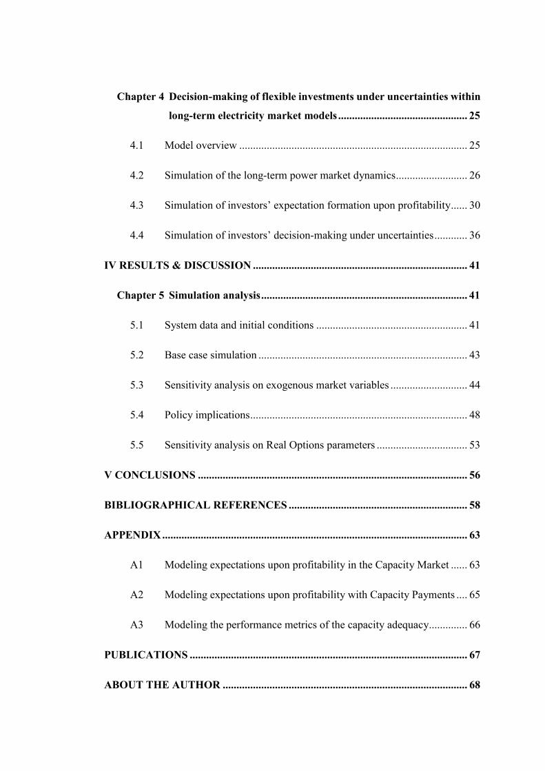
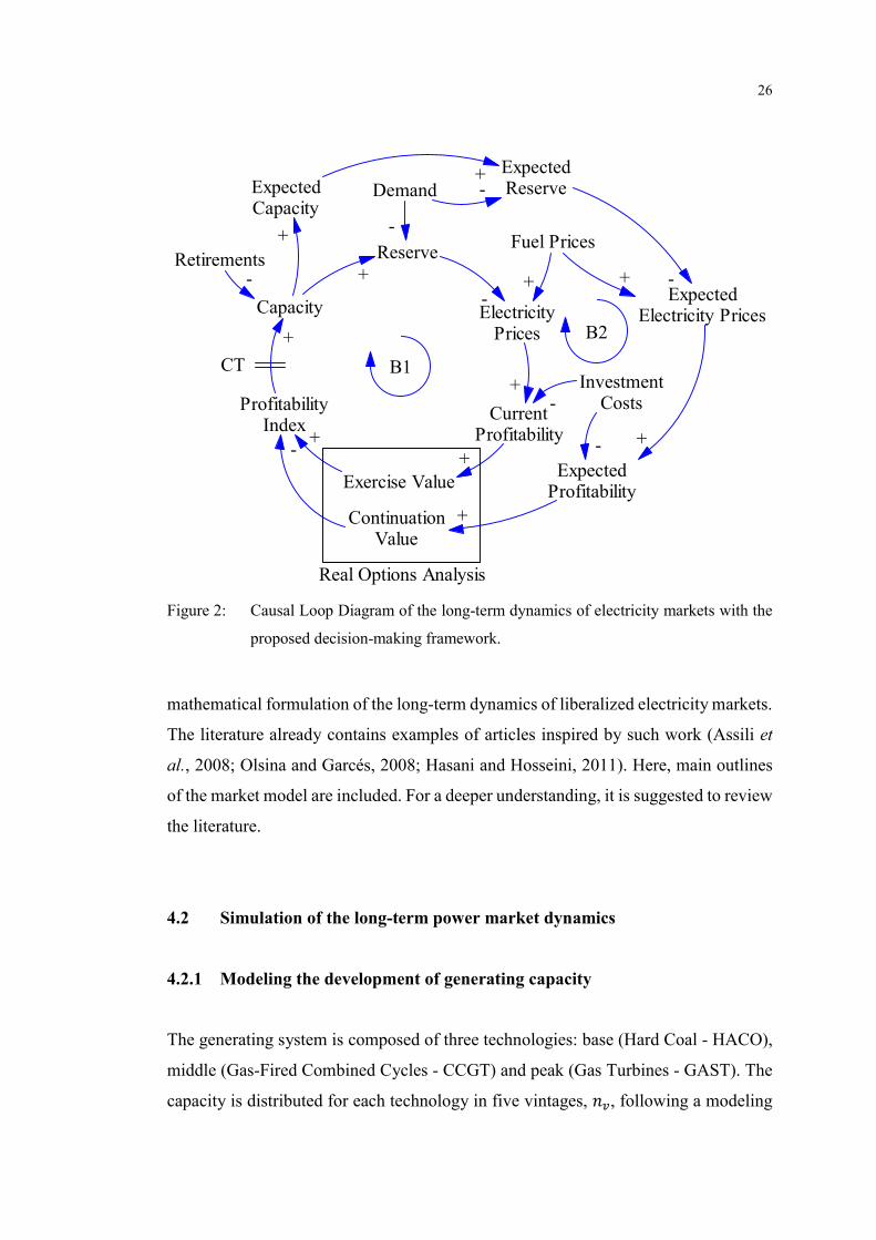
Figure 2 shows the Causal Loop Diagram (CLD) that explains the feedback structure

governing the long-term market development under the proposed decision-making

framework. Such diagram expands the CLD presented in Figure 1. First, investors

assess the prevailing market prices, based on the current state of installed capacity,

electricity demand and fuel prices, in order to estimate the profitability of undertaking

new generation projects immediately, i.e. the exercise value (loop B1). At the same

time, investors develop expectations upon future market prices, based on a stochastic

sample denoting the potential upcoming values of the same market parameters. By

means of Real Options (RO) analysis, these expectations are used to compute the

continuation value, that is, the project value if the decision is to postpone its execution,

waiting for more profitable conditions (loop B2). An investment profitability index is

then obtained from the ratio between the exercise value and the continuation value.

Such ratio determines the commissioning of new power plants, which come online,

however, only after a given Construction Time (CT). Finally, a new state of installed

capacity is defined by the existing capacity, the addition of new investments and the

decommissioning of old power plants that have accomplished their lifetime.

The model by Olsina et al. (2006) is used to assess the implementation of the proposed

investment valuation framework, since it is recognized for providing a comprehensive

26

Capacity

ProfitabilityIndex

Exercise Value

ContinuationValue

Retirements

+

-

-+

Reserve

Demand

ElectricityPrices

Fuel Prices

CurrentProfitability

+

-

-+

+

+

InvestmentCosts-

ExpectedCapacity

ExpectedReserve

+

+-

ExpectedElectricity Prices

-+

ExpectedProfitability

+-

+

B1

B2

Real Options Analysis

CT

Figure 2: Causal Loop Diagram of the long-term dynamics of electricity markets with the

proposed decision-making framework.

mathematical formulation of the long-term dynamics of liberalized electricity markets.

The literature already contains examples of articles inspired by such work (Assili et

al., 2008; Olsina and Garcés, 2008; Hasani and Hosseini, 2011). Here, main outlines

of the market model are included. For a deeper understanding, it is suggested to review

the literature.

4.2 Simulation of the long-term power market dynamics

4.2.1 Modeling the development of generating capacity

The generating system is composed of three technologies: base (Hard Coal - HACO),

middle (Gas-Fired Combined Cycles - CCGT) and peak (Gas Turbines - GAST). The

capacity is distributed for each technology in five vintages, ��, following a modeling

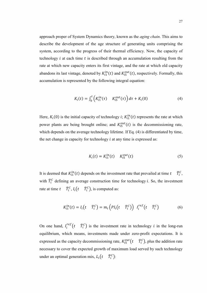
27

approach proper of System Dynamics theory, known as the aging chain. This aims to

describe the development of the age structure of generating units comprising the

system, according to the progress of their thermal efficiency. Now, the capacity of

technology � at each time � is described through an accumulation resulting from the

rate at which new capacity enters its first vintage, and the rate at which old capacity

abandons its last vintage, denoted by �����(�) and ���

���(�), respectively. Formally, this

accumulation is represented by the following integral equation:

��(�) = ∫ ������(�) ���

���(�)� ���

�+ ��(0) (4)

Here, ��(0) is the initial capacity of technology �; �����(�) represents the rate at which

power plants are being brought online; and ������(�) is the decommissioning rate,

which depends on the average technology lifetime. If Eq. (4) is differentiated by time,

the net change in capacity for technology � at any time is expressed as:

��(�) = �����(�) ���

���(�) (5)

It is deemed that �����(�) depends on the investment rate that prevailed at time � ���

�,

with ���� defining an average construction time for technology�. So, the investment

rate at time � ����, ���� ���

��, is computed as:

�����(�) = ���� ���

�� = �� ������ ������ ��

����� ���

�� (6)

On one hand, ������� ���

�� is the investment rate in technology � in the long-run

equilibrium, which means, investments made under zero-profit expectations. It is

expressed as the capacity decommissioning rate, �������� ���

��, plus the addition rate

necessary to cover the expected growth of maximum load served by such technology

under an optimal generation mix, ���� �����:

28

������� ���

�� = �������� ���

�� + ���� ����� (7)

On the other hand, the multiplier of the investment rate for technology �,

�� ������ ������, depends upon profitability expectations formed at time � ���

�.

Taking into account the system’s feedback structure, the expectation formation is

based on the prevailing balance of supply and demand, jointly with fuel prices. Hence,

the investment multiplier can be described as a function of the total capacity, demand

and fuel prices at such time:

�� ������ ������ = �� ����� ���

��, ��� �����, ���� ���

��� (8)

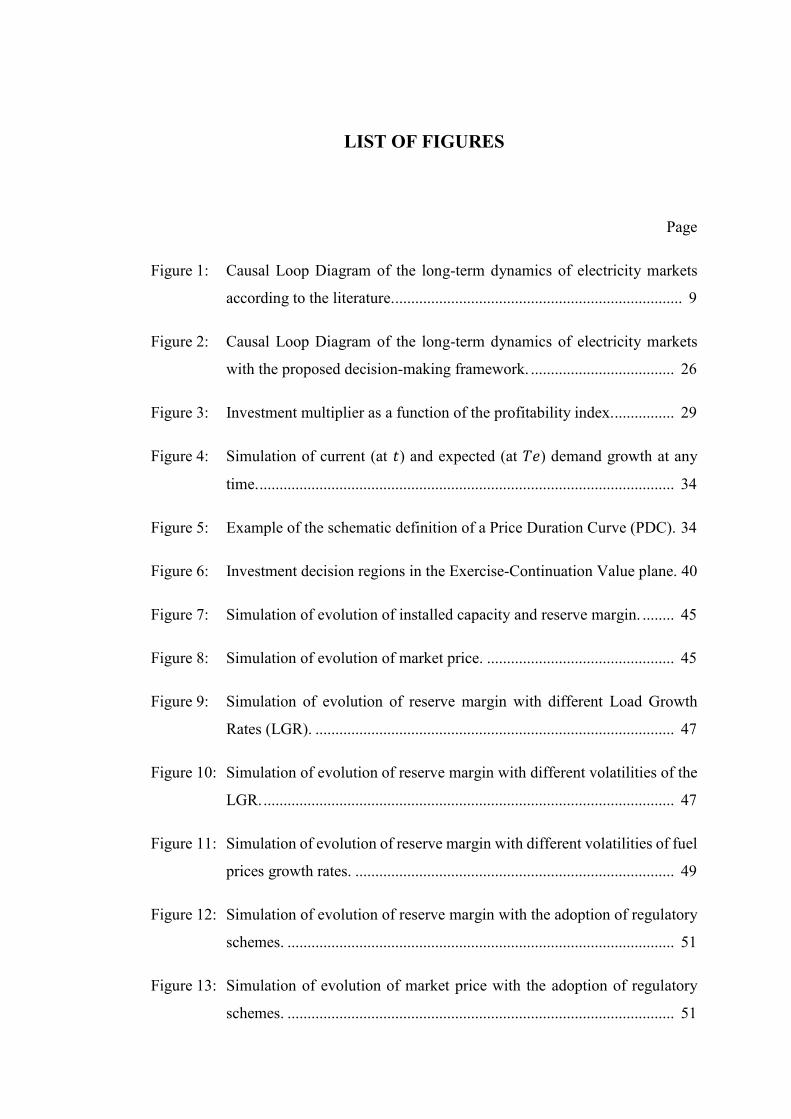
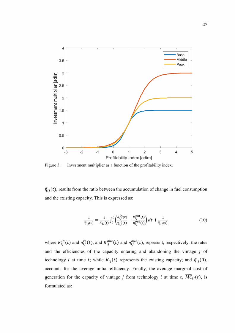
A logistic function is adopted for capturing the effect of the profitability index, ���, on

the multiplier of the investment rate for each technology �, ��. The three functions

employed in the context of the present study, one for each technology, are displayed

in Figure 3 (Olsina et al., 2006). Such curves are obtained from the following

expression:

��(�) =�����

������� ���(�)���� (9)

where ����� is the saturation level; �� controls the slope; and �� determines the

location of the function respect to the x-axis, for each technology �. The tipping point

in every case is given when the corresponding profitability index equals one.

4.2.2 Modeling the development of thermal efficiency

It is supposed that the average thermal efficiency of the generating system evolves

according to the efficiency progression and the development of capacity in each

vintage. Then, the average thermal efficiency for vintage � of technology � at time �,

29

-3 -2 -1 0 1 2 3 4 5

Profitability Index [adim]

0

0.5

1

1.5

2

2.5

3

3.5

4

Base

Middle

Peak

Figure 3: Investment multiplier as a function of the profitability index.

�̅��(�), results from the ratio between the accumulation of change in fuel consumption

and the existing capacity. This is expressed as:

�

����(�)=

�

���(�)∫ �

�����(�)

�����(�)

������(�)

������(�)

��

��� +

�

����(�) (10)

where �����(�) and ���

��(�), and ������(�) and ���

���(�), represent, respectively, the rates

and the efficiencies of the capacity entering and abandoning the vintage � of

technology � at time �; while ���(�) represents the existing capacity; and �̅��(0),

accounts for the average initial efficiency. Finally, the average marginal cost of

generation for the capacity of vintage � from technology � at time �, ���������(�), is

formulated as:

30

���������(�) =���(�)

����(�) (11)

In Eq. (11), ���(�) denotes the fuel price, and �̅��(�), the average thermal efficiency

for vintage � of technology � at time �.

4.3 Simulation of investors’ expectation formation upon profitability

4.3.1 Modeling expectations upon stochastic exogenous market variables

This thesis assumes that the market is driven exogenously by the demand and fuel

prices. Alongside with the installed capacity and fuel consumption, the assessment of

these variables is essential for investors when forming expectations upon profitability.

In that sense, this model computes the current and the expected state of such variables

at each step of the simulation horizon.

A deterministic growth pattern is assumed for describing the current state of demand

and fuel prices. Therefore, the maximum and minimum demand, and the fuel price for

technology �, at time � are formulated as:

����(�) = ����(0) ��� �; ����(�) = ����(0) �

�� � (12)

���(�) = ���(0) ����� � (13)

Here, ����(0) and ����(0) refer to the initial maximum and minimum demand, while

�� represents the annual growth rate in the long run. Accordingly, ���(0) denotes the

initial fuel price for technology �, and ���� is the annual rate driving its long-term

evolution.

The expected state of system variables at any time is characterized by a stochastic

evolution. In that sense, a mean-reverting stochastic process is prescribed for

31

describing the uncertain path of growth rates under consideration. This implies a

process where the uncertain variable evolves fluctuating around a known long-term

mean. A common mean-reverting process, known as the arithmetic Ornstein-

Uhlenbeck stochastic process, is given by:

�� = �(�̅ �)�� + ��� (14)

Here, the expected change in a growth rate, ��, after a time increment, ��, depends

upon the deviation from a long-run growth rate, �̅, and a speed of the reversion towards

the mean, �. It also depends upon a volatility parameter, �, and a variable following a

Wiener process, also known as Brownian Motion, ��. It can be shown that an

infinitesimal increment of the Wiener process, ��, is represented in continuous time

by:

�� = �√�� (15)

where � is a normally distributed random variable with mean zero and standard

deviation of 1, i.e. � = �(0,1).

In order to represent the market evolution in a more realistic way, the correlation

between, in one hand, the growth rates of demand and total installed capacity, and on

the other hand, prices of hard-coal and natural gas, is assumed. In that sense, the set of

random variables ��; � = 1,2, … ,� must be replaced by a set of correlated variables

��; � = 1,2, … , �. For computing the values of ��, the Cholesky decomposition is

applied to the correlation matrix, �, of the corresponding growth rates (Huang, 2009;

Pringles et al., 2015b):

� = ���� ���

��� ���

� = ��� (16)

32

In Eq. (16), � is a lower triangular matrix with elements ���; �, � = 1,2, … ,�, and ��

is the transpose matrix of �. Then, the value of ��; � = 1,2, … ,� is derived as the

linear combination of �, and the vector of independent variables �, which size is � ×

1:

���

��

� = �1 0

��� 1� × �

��

��� (17)

By writing Eq. (14) as a difference equation, Monte Carlo techniques can be applied

for simulating multiple stochastic realizations of correlated growth rates. Finally, a

realization � for the expected market parameters at time �� = � + ��, is derived by:

����� (��) = ����(�) �

��� ��; ����

� (��) = ����(�) ���� �� (18)

���(��) = ��(�) �

��� �� (19)

����(��) = ���(�) �

����� ��

(20)

On one hand, ����� (��) and ����

� (��) denote a realization of the expected maximum

and minimum demand at time ��, given a stochastic growth rate, ���. Furthermore, a

possible evolution of the total installed capacity is represented by ���(��), according

to a correlated growth rate, ��� . In that context, ��(�) is the total capacity of the system

at time �, which results from the dynamic model described in the previous subsection.

On the other hand, ����(��) illustrates a realization of the expected fuel price of

technology � at time ��, given a stochastic growth rate, ����� . Similarly to the case of

demand and installed capacity, the growth rates of prices for both technologies are

correlated to each other.

The modeling approach presented here assumes that the aforementioned market

variables are observable for each investor at any time � within the simulation horizon.

Such parameters are therefore described by means of constant growth rates, aiming to

33

characterize the development of the market in the long term. Notwithstanding, it is

supposed that investors are equally concerned about the ongoing uncertainties that

might divert the future growth rates from their average values. Thus, by using the

observable values at each time, the proposed model allows computing a stochastic

sample of future market variables. These parameters are employed in order to form

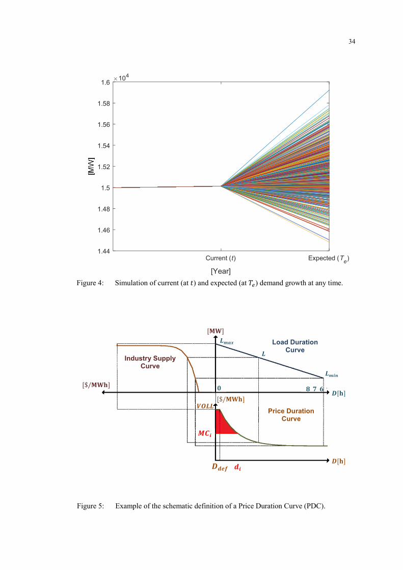
each investor’s expectations upon profitability at an expiration time �� = � + ��. An

example of the simulation of current (at time �) and expected (at time �� = � + ��)

values for the demand growth at any time is illustrated in Figure 4.

4.3.2 Modeling expectations upon operating profits

A price duration model, based on a probabilistic Price Duration Curve (PDC), is used

for deriving the current and the expected short-term, infra-marginal revenue being

perceived at each time by each technology, and thereby the market signals for decision-

making of new power plants. In order to define the appropriate PDC for each case, the

corresponding market variables, both at time �, and at time �� = � + ��, are taken into

account, by following the outlines exposed in the previous subsection.

Each PDC is computed schematically from a Load Duration Curve (LDC), jointly with

an industry supply curve. An example of such definition is included in Figure 5. First,

the LDC determines the annual probability for the system demand to equal or exceed

a certain level between its maximum and minimum values. In that sense, it is assumed

that the LDC accounts for a linear distribution, preserving such pattern over the entire

simulation horizon. Second, the industry supply curve defines the costs of supplying

to the different levels of system demand. This curve results from sorting the capacity

available in each vintage of the system following an economic dispatch merit order,

that is, according to their respective marginal cost of generation, from lower to higher.

The availability of capacity for each vintage is computed by means of a probabilistic

model, which accounts for the reliability of generating units, and the variability of

electricity demand (Olsina et al., 2006).

34

Current (t) Expected (Te)

[Year]

1.44

1.46

1.48

1.5

1.52

1.54

1.56

1.58

1.6104

Figure 4: Simulation of current (at �) and expected (at ��) demand growth at any time.

����

�

[��]

Industry Supply Curve

[$/���]

[$/���] ����

�

����

����

Load Duration Curve

�[�]

���

���� �[�]

Price Duration Curve

��

Figure 5: Example of the schematic definition of a Price Duration Curve (PDC).

35

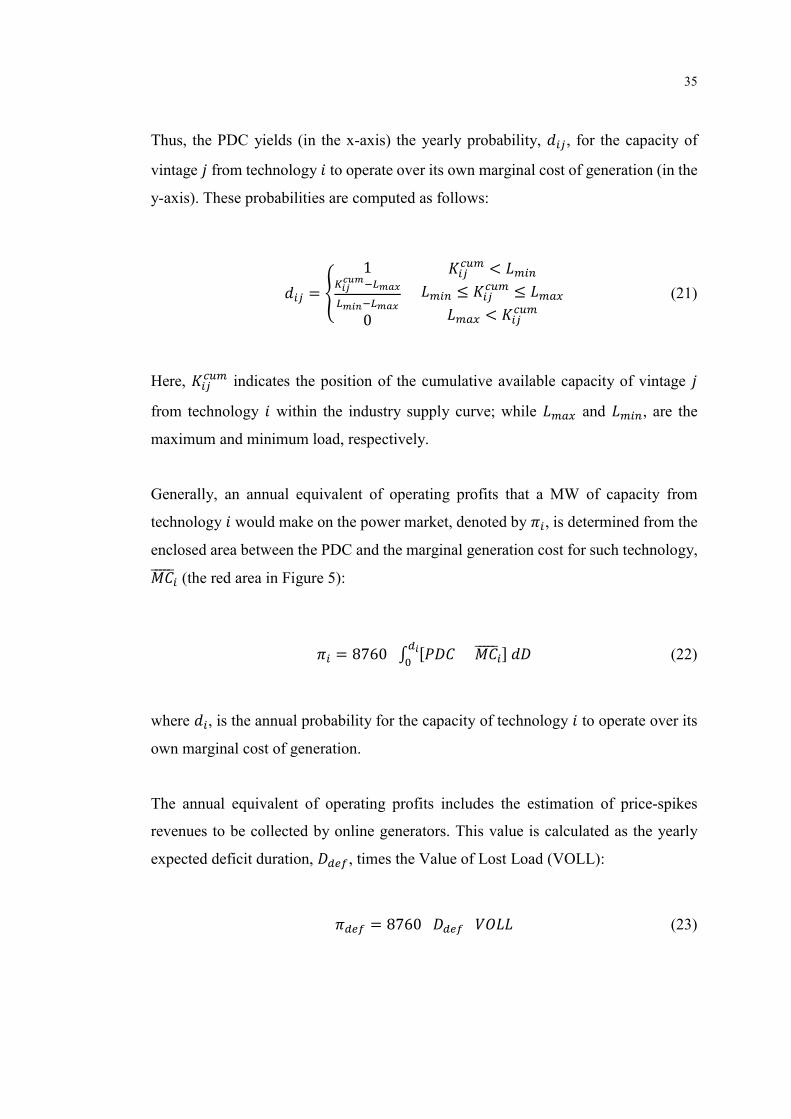
Thus, the PDC yields (in the x-axis) the yearly probability, ���, for the capacity of

vintage � from technology � to operate over its own marginal cost of generation (in the

y-axis). These probabilities are computed as follows:

��� = �

1�����������

���������

0

������ < ����

���� ≤ ������ ≤ ����

���� < ������

(21)

Here, ������ indicates the position of the cumulative available capacity of vintage �

from technology � within the industry supply curve; while ���� and ����, are the

maximum and minimum load, respectively.

Generally, an annual equivalent of operating profits that a MW of capacity from

technology � would make on the power market, denoted by ��, is determined from the

enclosed area between the PDC and the marginal generation cost for such technology,

�������� (the red area in Figure 5):

�� = 8760 ∫ [��� ��������]�����

(22)

where ��, is the annual probability for the capacity of technology � to operate over its

own marginal cost of generation.

The annual equivalent of operating profits includes the estimation of price-spikes

revenues to be collected by online generators. This value is calculated as the yearly

expected deficit duration, ����, times the Value of Lost Load (VOLL):

���� = 8760 ���� ���� (23)

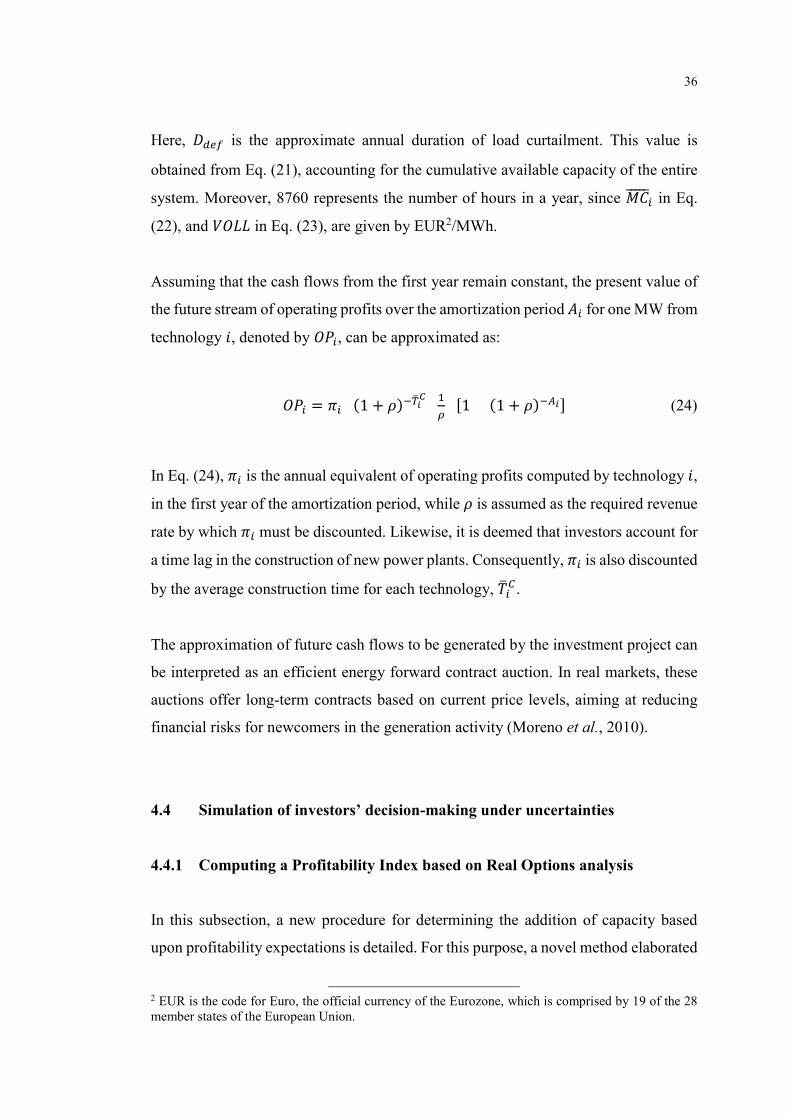
36

Here, ���� is the approximate annual duration of load curtailment. This value is

obtained from Eq. (21), accounting for the cumulative available capacity of the entire

system. Moreover, 8760 represents the number of hours in a year, since �������� in Eq.

(22), and ���� in Eq. (23), are given by EUR2/MWh.

Assuming that the cash flows from the first year remain constant, the present value of

the future stream of operating profits over the amortization period �� for one MW from

technology �, denoted by ���, can be approximated as:

��� = �� (1 + �)����

� �

�[1 (1 + �)���] (24)

In Eq. (24), �� is the annual equivalent of operating profits computed by technology �,

in the first year of the amortization period, while � is assumed as the required revenue

rate by which �� must be discounted. Likewise, it is deemed that investors account for

a time lag in the construction of new power plants. Consequently, �� is also discounted

by the average construction time for each technology, ����.

The approximation of future cash flows to be generated by the investment project can

be interpreted as an efficient energy forward contract auction. In real markets, these

auctions offer long-term contracts based on current price levels, aiming at reducing

financial risks for newcomers in the generation activity (Moreno et al., 2010).

4.4 Simulation of investors’ decision-making under uncertainties

4.4.1 Computing a Profitability Index based on Real Options analysis

In this subsection, a new procedure for determining the addition of capacity based

upon profitability expectations is detailed. For this purpose, a novel method elaborated

2 EUR is the code for Euro, the official currency of the Eurozone, which is comprised by 19 of the 28 member states of the European Union.

37

upon the notion of RO analysis is proposed. This is the main contribution of this work,

since it focuses on integrating a RO-based framework for valuing power plants under

uncertainties within a long-term dynamic market model.

Rigorously, an optimal investment policy for each technology at each time can be

derived by comparing the intrinsic value of immediately undertaking new generation

projects with the value of keeping alive the postponement option. Backward Dynamic

programming based on Expected Present value (DPE) is a suitable tool for performing

this task (Blanco et al., 2012). Moreover, it has been verified experimentally that the

DPE allows avoiding problems related to applying other dynamic programming tools

(e.g. the binomial lattice method), for instance, when dealing with highly-volatile

future profits, as in this study case.

In that context, the exercise value for technology �, ����(�), is defined by the Net

Present Value (NPV) of new generation projects, according to the current state of the

system at time �. This can be expressed as:

����(�) = ���(�) ��(�) (25)

where ���(�) is the present value of cumulated operating profits perceived by

technology � at time �; and ��(�) represents the capital outlay for bringing online a new

generator of technology � at the same time.

On the other hand, an expiration time is used to represent the future threshold when

the execution of the project must be reassessed, if the decision is to postpone it. At the

expiration time, equal to �� = � + ��, the decision problem for technology � can be

therefore modeled as:

��������, ����(��) = �[���(��)] > ��(��) (26)

�������������, ����(��) = �[���(��)] ≤ ��(��)

38

Exercise Value Continuation Value

Thus, the optimal investment policy for technology � at time ��, �� (��), can be defined

as:

�� (��) = ������[���(��)] ��(��)�; 0� (27)

On one hand, �[���(��)] denotes the expected present value of cumulated operating

profits for technology � at time ��, which is obtained based on the stochastic sample

of expected market conditions at such time. On the other hand, ��(��) represents the

investment costs expected for the same technology at time ��.

By considering only a single period, ��, between the current and the expiration time,

the continuation value of the postponement option for technology � at time �, i.e. the

project value if the decision is to postpone its execution, ������(�), can be expressed

as:

������(�) =

�� (��)(1 + �)��� (28)

where � represents a risk-free discount rate. According to the implementation of the

DPE method, this value is equal to a hurdle discount rate3, which adjustment follows

a non-neutral valuation of risk.

The optimal investment policy for technology � at each time �, �� (�), can be then

derived from the following optimization problem (Blanco et al., 2012):

�� (�) = max �����,�(�) ��(�); �� (��)

(1 + �)��� � (29)

3 The hurdle discount rate can be understood as the Weighted Average Cost of Capital (WACC) of investment projects.

39

As mentioned by Blanco et al. (2012), the relationship given by Eq. (29) allows

extending the conventional NPV-based rule for characterizing the feasibility of new

projects. In that sense, a new investment decision threshold can be defined as follows:

“At time �, the decision-maker should not invest in a new project (and wait for

reassessing it after a given period ��) unless the current NPV of the investment

portfolio (the Exercise Value) is greater than the Continuation Value”.

Accordingly, a new investment profitability index (PI) for technology � at time � can

be defined as the ratio resulting from dividing the exercise value, ����(�), by the

continuation value, ������(�):

���(�) =����(�)

������(�)

� (30)

Finally, this profitability index is set to determine the addition of new investments

within the dynamic model, which is adopted in order to analyze the long-term

development of the liberalized electricity market.

4.4.2 Investor responsiveness under uncertainties

It is worth to notice that, under this new framework, the attractiveness of undertaking

investments, as a function of the PI, can be described schematically, as in Figure 6

(Luehrman, 1998). Whenever the exercise value is positive and it exceeds the

continuation value, the optimal strategy should be to invest now (Region 1). However,

when the exercise value does not exceed the continuation value, the investor would be

cautious about the market’s uncertain conditions and would probably reconsider to

invest later (Region 2).

It is intuitive to assume that the project appraisal will be much more pessimistic

whenever its instant NPV is negative. In that context, it is natural for each generator

to withhold investments until new information about the market evolution arrives

(Region 3). Moreover, when the exercise value is negative, and its absolute exceeds

40

Figure 6: Investment decision regions in the Exercise-Continuation Value plane.

the continuation value, there would be no incentives to invest whatsoever (Region 4).

In this case, the investor could even consider switching of business.

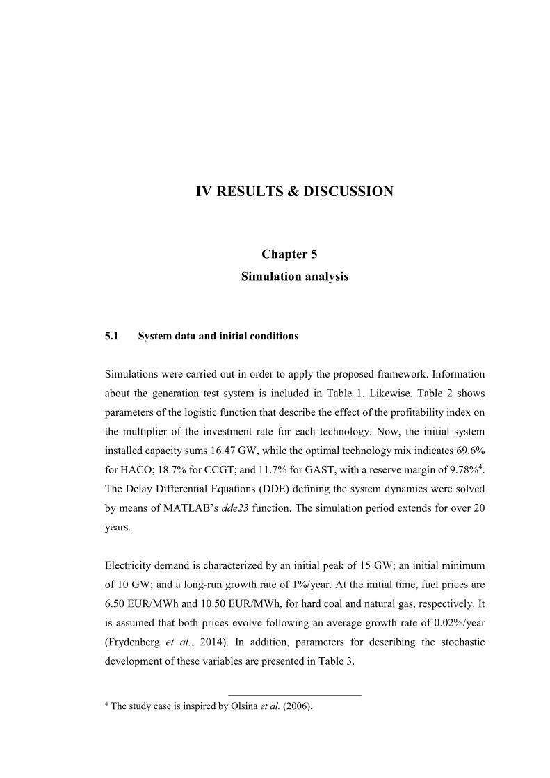
IV RESULTS & DISCUSSION

Chapter 5

Simulation analysis

5.1 System data and initial conditions

Simulations were carried out in order to apply the proposed framework. Information

about the generation test system is included in Table 1. Likewise, Table 2 shows

parameters of the logistic function that describe the effect of the profitability index on

the multiplier of the investment rate for each technology. Now, the initial system

installed capacity sums 16.47 GW, while the optimal technology mix indicates 69.6%

for HACO; 18.7% for CCGT; and 11.7% for GAST, with a reserve margin of 9.78%4.

The Delay Differential Equations (DDE) defining the system dynamics were solved

by means of MATLAB’s dde23 function. The simulation period extends for over 20

years.

Electricity demand is characterized by an initial peak of 15 GW; an initial minimum

of 10 GW; and a long-run growth rate of 1%/year. At the initial time, fuel prices are

6.50 EUR/MWh and 10.50 EUR/MWh, for hard coal and natural gas, respectively. It

is assumed that both prices evolve following an average growth rate of 0.02%/year

(Frydenberg et al., 2014). In addition, parameters for describing the stochastic

development of these variables are presented in Table 3.

4 The study case is inspired by Olsina et al. (2006).

42

Table 1: Input data for the generation test system.

Technology HACO CCGT GAST

Capacity [MW] 11460 3080 1930

Construction delay [month] 36 18 9

Lifetime [year] 40 30 20

Amortization period [year] 25 20 15

Investment costs [EUR/kW] 1000 600 300

Fuel costs [EUR/MWh] 6.50 10.50 10.50

Discount rate [%/year] 12.5 12.5 12.5

Table 2: Parameters of the logistic function for the multiplier of the investment rate for

each technology.

Parameter HACO CCGT GAST

Saturation, ����� 1.50 3.00 2.00

Alpha, �� 3.50 2.00 2.50

Beta, �� -2.8069 -2.6932 -2.500

Table 3: Parameters to characterize the stochastic growth rates of maximum and minimum

demand (��), total installed capacity (��), fuel price of hard-coal (���,����) and

fuel price of natural gas (���,���).

Parameter �� �� ���,���� ���,���

Initial growth rate [%/year] 1.00 1.00 0.02 0.02

Long-term growth rate [%/year] 1.00 1.00 0.02 0.02

Speed of reversion [%/year] 50.0 50.0 50.0 50.0

Volatility [%/year] 2.00 2.00 1.85 3.95

Correlation [dmnl] 0.80 0.80 0.71 0.71

The number of Monte Carlo realizations is 50,000, in order to satisfy convergence

criteria in the statistical estimation of the expected value of future profits.

43

The RO investment valuation model considers European options with an expiration

time, ��, equal to one year for each technology. Likewise, a hurdle discount rate equal

to 12.5%/year is adopted for each technology. This value indicates a risk-free discount

rate, adjusted following a non-neutral valuation. Finally, the Value of Lost Load

(VOLL) is set to 1000 EUR/MWh.

5.2 Base case simulation

In Figure 7, the simulation of evolution of installed capacity and reserve margin in the

test system is plotted, jointly with the expected value of peak demand. Results are

relevant because it is observed that the proposed investment valuation approach allows

reproducing explicitly the construction cycles that have occurred in several electricity

markets after the liberalization (Arango and Larsen, 2011). This is explained due to

the more refined characterization of investors’ decision-making under uncertainties, in

addition to the embedded construction delays for new power plants of each technology.

The system response is described as follows. Given the zero-profit conditions at the

beginning of simulations, i.e. long-run market equilibrium, the continuation value

outweighs the exercise value of power plants for each technology. Thus, generators

find more attractive to withhold new projects because they have the possibility to

invest later and collect extraordinary profits associated to situations of supply deficit

(Region 2 and Region 3 in Figure 6). This leads to a dramatic reduction of reserve

margins during the first years, just after the liberalization of the electricity market.

Notwithstanding, it is worth to mention that such reduction displays a discontinuous

behavior. An explanation is that the completion rate lag the investment rate by the

construction time for each technology. Therefore, during the period � ≤ ����, power

plants are still being completed according to the ordering rate given under the long-

run market equilibrium. Only after � > max������, the aggregate completion rate start

to reflect investment rates resulting from the commercial decisions of investors in each

technology. Then, the evolution of installed capacity and reserve margin begins to

display a continuous behavior.

44

The installed capacity decreases until reaching an extremely low value around year 4,

when the investment exercise is finally able to surpass the continuation value for each

technology. Only then it becomes attractive to invest now due to the high revenues

being perceived thanks to the critical supply condition (Region 1 of Figure 6). A stream

of new units is thereby incorporated to the system, and remains until the continuation

value begins to surpass the exercise value once again, due to the excess of capacity,

around year 14. The construction cycle then starts over once more.

This remarkable fluctuating behavior impacts on the electricity prices that must be paid

by consumers. In Figure 8, the annual-average market prices simulated under the

proposed framework are depicted. According with the alerted cyclical behavior, the

Real-Options-based case derives a market affected by significant price spikes,

coincident with the critical reduction of installed capacity.

5.3 Sensitivity analysis on exogenous market variables

5.3.1 Mean of demand growth rate

A sensitivity analysis was carried out respect to the mean of demand growth rate. In

that sense, the simulation of capacity adequacy with long-term load growth rates of

0%/year and 2%/year is depicted in Figure 9. Initially, it is verified that the system

shows a more dramatic reduction of reserve margins with higher growth rates. An

explanation is that increased growth rates yield greater expectations upon deficit

conditions in the short term for each technology. Hence, the continuation value

severely outweighs the exercise value, and investors constrain even more the addition

of new capacity.

When investment exercise becomes attractive, it is observed that the stream of new

power plants is incorporated to the system at a higher rate, for higher growth rates.

This would cause later a pronounced situation of capacity excess, which would define

45

0 2 4 6 8 10 12 14 16 18 20

[Year]

1

1.1

1.2

1.3

1.4

1.5

1.6

1.7

1.8

1.9

2104

0

2

4

6

8

10

12

14

16

18

20

Installed Capacity

Peak Demand

Reserve Margin

Figure 7: Simulation of evolution of installed capacity and reserve margin.

0 2 4 6 8 10 12 14 16 18 20

[Years]

10

20

30

40

50

60

70

Prod. Cost

Market Price

Figure 8: Simulation of evolution of market price.

46

again the start of a new construction cycle, but of increased amplitude. Therefore, it is

reasonable to predict a more volatile market condition as the demand growth rate

increases.

5.3.2 Volatility of demand growth rate

Figure 10 shows the simulation of capacity adequacy for different volatilities of the

demand growth rate. With higher volatilities, it is found that the market experiences a

more dramatic depletion of reserve margins along the first years. As in the previous

example, this is explained because the higher the volatility, the more likely the deficit

conditions that imply extraordinary profits in the short term for each technology.

After the first drop of reserve margins, the market with lower volatilities needs to reach

an overstepped capacity situation for the continuation value to exceed once again the

investment exercise value for each technology. This behavior is explained due to the

fewer uncertainties about the market evolution, which leads to the reduction of the

continuation value and gives the signal to invest in more power plants than required.

Later on, this leads to a more dramatic reduction of reserve margins, which impacts

directly on the stability of market prices.

On the opposite side, fewer investments are required to be added for the continuation

value of each technology to surpass again the exercise value in a highly-volatile

scenario. Despite the more stable market behavior, this means that the reserve margin

is constantly below the economic optimum, which settles the market clearing prices

on a rather high average value. An explanation is that investors are likely to execute

new projects proportionally in order to maintain a low reserve margin and secure high

deficit profits, in response to expectations upon a highly uncertain market evolution.

The described patterns are coherent with the experience in actual electricity markets.

In fact, lessons learned suggest that the combination of strong demand growth rates,

with high volatilities, was one of the main reasons that led to crises in supply security

47

0 2 4 6 8 10 12 14 16 18 20

[Years]

2

3

4

5

6

7

8

9

10

LGR = 1 %/year

LGR = 0 %/year

LGR = 2 %/year

0 2 4 6 8 10 12 14 16 18 20

[Years]

0

2

4

6

8

10

= 2.00 %/year

= 0.50 %/year

= 1.00 %/year

= 4.00 %/year

= 8.00 %/year

Figure 10: Simulation of evolution of reserve margin with different volatilities of the LGR.

Figure 9: Simulation of evolution of reserve margin with different Load Growth Rates

(LGR)

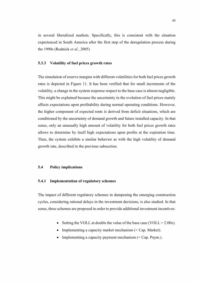
48

in several liberalized markets. Specifically, this is consistent with the situation

experienced in South America after the first step of the deregulation process during

the 1990s (Rudnick et al., 2005)

5.3.3 Volatility of fuel prices growth rates

The simulation of reserve margins with different volatilities for both fuel prices growth

rates is depicted in Figure 11. It has been verified that for small increments of the

volatility, a change in the system response respect to the base case is almost negligible.

This might be explained because the uncertainty in the evolution of fuel prices mainly

affects expectations upon profitability during normal operating conditions. However,

the higher component of expected rents is derived from deficit situations, which are

conditioned by the uncertainty of demand growth and future installed capacity. In that

sense, only an unusually high amount of volatility for both fuel prices growth rates

allows to determine by itself high expectations upon profits at the expiration time.

Then, the system exhibits a similar behavior as with the high volatility of demand

growth rate, described in the previous subsection.

5.4 Policy implications

5.4.1 Implementation of regulatory schemes

The impact of different regulatory schemes in dampening the emerging construction

cycles, considering rational delays in the investment decisions, is also studied. In that

sense, three schemes are proposed in order to provide additional investment incentives:

Setting the VOLL at double the value of the base case (VOLL = 2.00x).

Implementing a capacity market mechanism (+ Cap. Market).

Implementing a capacity payment mechanism (+ Cap. Paym.).

49

0 2 4 6 8 10 12 14 16 18 20

[Years]

2

3

4

5

6

7

8

9

10

= 1.00x

= 8.00x

= 16.00x

= 32.00x

Figure 11: Simulation of evolution of reserve margin with different volatilities of fuel prices

growth rates.

On one hand, the VOLL is a key variable which setting is within reach of regulators.

It is deemed that a higher VOLL might help in timely undertaking new power plants

because investors would perceive a higher profit in the energy-only market without

arriving to a severe deficit situation. On the other hand, the capacity market and the

capacity payment are regulatory mechanisms that intend to remunerate generators

separately from the energy-only market. In that sense, the formulation of the additional

revenues to be expected by each technology is given in detail in the Appendix. Such

profits must be eventually summed to Eq. (22) in order to determine the full expected

profitability for each technology with the implementation of each regulatory scheme.

At each time, it is assumed that the existing capacity participates entirely in the

capacity market, while only the base technology makes bids of new capacity. It is

supposed that these offers are always equal to the 15% of the instant system capacity

50

(Hary et al., 2016). The target system capacity is given by the observable peak demand

and the target optimal reserve margin, which is equal to 9.78%.

Accordingly, the LOLP necessary to compute the capacity payment is derived from

the annual-average system availability. It remains constant over the simulation

horizon, and is based on the optimal deficit duration, according to the system’s initial

conditions.

Results for the simulated reserve margin are included in Figure 12, while the simulated

market prices are depicted in Figure 13.

5.4.2 Performance of the capacity adequacy

Two metrics are adopted to characterize the performance of capacity adequacy over

the simulation horizon. First, the Root Square Mean Error (RSME) to the Target

Reserve Margin (TRM) is used to indicate the degree of supply security. Next, the

signal of economic performance is given by a so-called Annual-average Unitary

Expenditure (AUE). It denotes the yearly equivalent amount that consumers would

have paid for each MW of the system, over the average production costs, during the

entire simulation horizon. This value can be computed from the enclosed area between

the simulated market price and the corresponding production costs. For the sake of

clarity, the mathematical expression for both metrics is included in the Appendix.

The performance of each market design according to the proposed metrics is illustrated

in Figure 14. Numerical values are provided in Table 4. It is verified that the capacity

payment mechanism offers the best performance regarding the security of supply.

Nevertheless, this happens at expense of an extremely high profit for investors. From

the point of view of consumers, the energy-only market derives a much more moderate

amount of expenditure. However, in that case, there is a higher risk of deviating from

the target reserve margin, even with the increase in the VOLL, affecting the security

of supply.

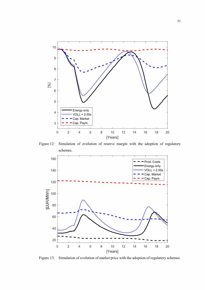
51

0 2 4 6 8 10 12 14 16 18 20

[Years]

3

4

5

6

7

8

9

10

Energy-only

VOLL = 2.00x

Cap. Market

Cap. Paym.

0 2 4 6 8 10 12 14 16 18 20

[Years]

20

40

60

80

100

120

140

160Prod. Costs

Energy-only

VOLL = 2.00x

Cap. Market

Cap. Paym.

Figure 13: Simulation of evolution of market price with the adoption of regulatory schemes.

Figure 12: Simulation of evolution of reserve margin with the adoption of regulatory

schemes.

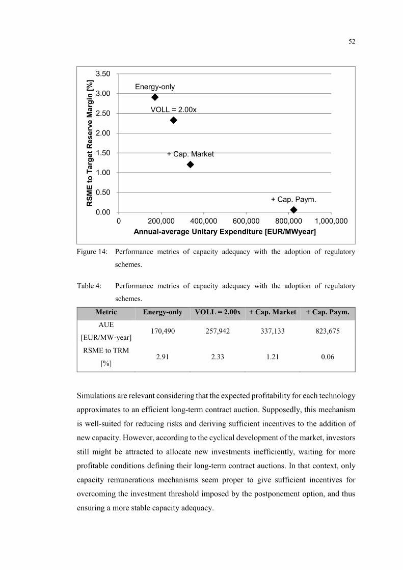
52

Energy-only

VOLL = 2.00x

+ Cap. Market

+ Cap. Paym.

0.00

0.50

1.00

1.50

2.00

2.50

3.00

3.50

0 200,000 400,000 600,000 800,000 1,000,000

RS

ME

to

Ta

rge

t R

es

erv

e M

arg

in [

%]

Annual-average Unitary Expenditure [EUR/MWyear]

Figure 14: Performance metrics of capacity adequacy with the adoption of regulatory

schemes.

Table 4: Performance metrics of capacity adequacy with the adoption of regulatory

schemes.

Metric Energy-only VOLL = 2.00x + Cap. Market + Cap. Paym.

AUE

[EUR/MW·year] 170,490 257,942 337,133 823,675

RSME to TRM

[%] 2.91 2.33 1.21 0.06

Simulations are relevant considering that the expected profitability for each technology

approximates to an efficient long-term contract auction. Supposedly, this mechanism

is well-suited for reducing risks and deriving sufficient incentives to the addition of

new capacity. However, according to the cyclical development of the market, investors

still might be attracted to allocate new investments inefficiently, waiting for more

profitable conditions defining their long-term contract auctions. In that context, only

capacity remunerations mechanisms seem proper to give sufficient incentives for

overcoming the investment threshold imposed by the postponement option, and thus

ensuring a more stable capacity adequacy.

53

5.5 Sensitivity analysis on Real Options parameters

5.5.1 Expiration time

The impact of different expiration times is also subject of discussion. It is worth to

recognize that the expiration time, also known as the option maturity, conventionally

denotes a threshold after which investments can no longer be undertaken. Due to the

irreversibility, this might derive in conveniently setting different expiration times for

each generating technology. Therefore, here it is assumed that investors might consider

investment expiration times equal to the multiple of 36, 18 and 9 months for HACO,

CCGT and GAST, respectively. On one hand, this setting explains that investors in

base technologies will be more cautious about the market uncertain development due

to the higher sunk costs. On the other hand, investors in peak technologies will not be

prone to delay investments excessively because of the lower irreversibility. The

simulated scenarios are presented in Table 5.

Results are shown in Figure 15. It is observed that the simulations with disaggregated

option maturities exhibit a more significant reduction of reserve margins in the first

years respect to the base case. This is explained due to the longer expiration times for

base technologies, which results in market uncertainties determining even more

profitable conditions if the decision is to postpone investments. This leads to a rapid

reduction of reserve margins because of the insufficient addition of base capacity,

which accounts for the greatest proportion of capacity within the system energy mix.

Furthermore, it is verified that the market with disaggregated maturities requires fewer

investments for the continuation value to exceed the exercise value once again. This

implies the setting of market prices on higher average values, representing the strategic

behavior of base investors in response to increased uncertainties at the maturity. The

situation also determines the reduction of the period in the construction cycles, which

leads to an increased instability of the market development, when considering a higher

irreversibility for base power investments.

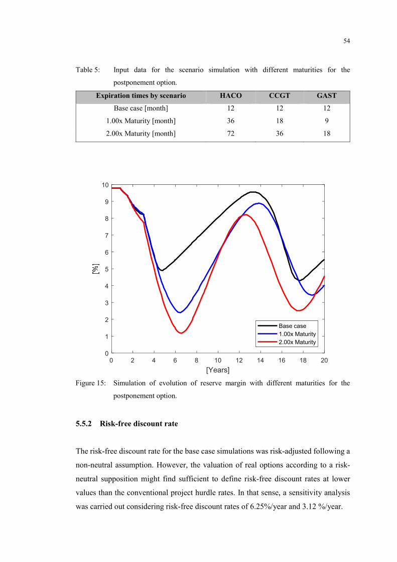
54

0 2 4 6 8 10 12 14 16 18 20

[Years]

0

1

2

3

4

5

6

7

8

9

10

Base case

1.00x Maturity

2.00x Maturity

Figure 15: Simulation of evolution of reserve margin with different maturities for the

postponement option.

Table 5: Input data for the scenario simulation with different maturities for the

postponement option.

Expiration times by scenario HACO CCGT GAST

Base case [month] 12 12 12

1.00x Maturity [month] 36 18 9

2.00x Maturity [month] 72 36 18

5.5.2 Risk-free discount rate

The risk-free discount rate for the base case simulations was risk-adjusted following a

non-neutral assumption. However, the valuation of real options according to a risk-

neutral supposition might find sufficient to define risk-free discount rates at lower

values than the conventional project hurdle rates. In that sense, a sensitivity analysis

was carried out considering risk-free discount rates of 6.25%/year and 3.12 %/year.

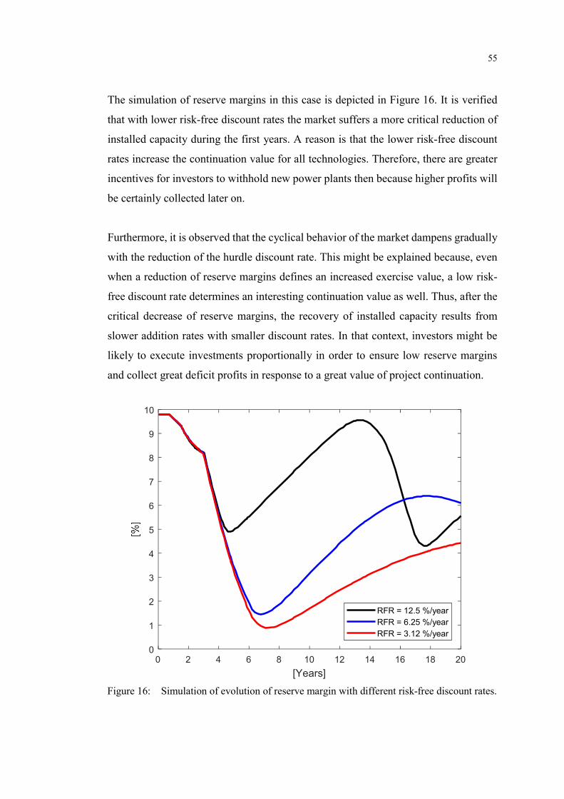
55

0 2 4 6 8 10 12 14 16 18 20

[Years]

0

1

2

3

4

5

6

7

8

9

10

RFR = 12.5 %/year

RFR = 6.25 %/year

RFR = 3.12 %/year

Figure 16: Simulation of evolution of reserve margin with different risk-free discount rates.

The simulation of reserve margins in this case is depicted in Figure 16. It is verified

that with lower risk-free discount rates the market suffers a more critical reduction of

installed capacity during the first years. A reason is that the lower risk-free discount

rates increase the continuation value for all technologies. Therefore, there are greater

incentives for investors to withhold new power plants then because higher profits will

be certainly collected later on.

Furthermore, it is observed that the cyclical behavior of the market dampens gradually

with the reduction of the hurdle discount rate. This might be explained because, even

when a reduction of reserve margins defines an increased exercise value, a low risk-

free discount rate determines an interesting continuation value as well. Thus, after the

critical decrease of reserve margins, the recovery of installed capacity results from

slower addition rates with smaller discount rates. In that context, investors might be

likely to execute investments proportionally in order to ensure low reserve margins

and collect great deficit profits in response to a great value of project continuation.

V CONCLUSIONS

After developing this research work, it is concluded that a novel decision-making

framework to assess the long-run capacity adequacy in liberalized power markets has

been proposed. The designing of the methodology has taken advantage of a well-

founded background for simulating the long-term market dynamics, based on a System

Dynamics simulation approach. However, the proposed research work is different as

it has focused on modeling the investors’ decision-making process, accounting for the

strategic flexibility of generation investments under uncertainties. For this purpose, a

new investment valuation framework, elaborated by means of Real Options analysis,

has been presented.

In that context, the simulation of multiple scenarios for depicting the market uncertain

evolution has allowed to quantify the value of postponing new power plants in order

to be reconsidered later. At each time, a new profitability index has been obtained by

relating such continuation value with the value of undertaking the investment

immediately. This relation has ultimately defined the entrance of new capacity for each

generating technology.

Results have shown that with the proposed model the long term market development

has been defined by explicit construction cycles. Several sensitivity analyses respect

to key market variables has been performed in order to test the robustness of the

described framework. In that sense, it has been suggested that the combination of

strong demand growth rates with large volatilities would derive an even more volatile

evolution of installed capacity. Likewise, the new Real- Options-based methodology

57

has been applied to assess the implementation of three different regulatory schemes

intended to dampen the perceived construction cycles. Simulations have illustrated

that, for ensuring the supply security, higher incentives must be offered in order to

counteract the investor’s behavior when deciding strategic projects under uncertainty.

Likewise, the impact of different maturity horizons and hurdle discount rates has been

explored. In that sense, it has been verified that an increase in the expiration times for

base technologies, due to the irreversibility, would determine an even more unstable

market development. Furthermore, the reduction of the hurdle discount rate might

suppress the perceived construction cycles, but at expense of significantly narrowing

the market reserve margins, because of the increased value of investment continuation.

The cyclical investment pattern depicted in this research work has reproduced the

empirical evidence that have been reported by several electricity markets after the

deregulation. In that sense, the main contribution of this work has been a rigorous

mathematical description of the origins of this phenomenon. This might help in the

design of investment incentives, suitable for deriving a stable development of the

liberalized power industry in the long term.

The following points will be included in further research:

Critical review of the expectation formation model: The possibility of multiple

paths for describing the uncertain evolution of the observable market variables

will be considered from the beginning of the simulation horizon.

Application of other Real Option methods: The impact of using binomial lattices

or stochastic simulation models, like Least-Square Monte Carlo techniques, will

be considered for valuing the American type of real options in the decision-

making of each technology.

Incorporation of non-thermal generating technologies: The generation test

system will be expanded, in order to include further generating technologies,

especially, renewables. This will help in studying the impact of large-scale

integration of renewable energy, which is now center of interest.

BIBLIOGRAPHICAL REFERENCES

ABANI, A. O., HARY, N., SAGUAN, M., & RIOUS, V. (2016). Risk aversion and generation adequacy in liberalized electricity markets: benefits of capacity markets. 2016 IEEE International Conference on the European Energy Market, (pp. 1-5). Porto, PT.

AHMAD, S., TAHAR, R. M., MUHAMMAD-SUKKI, F., MUNIR, A. B., & RAHIM, R. A. (2016). Application of System Dynamics approach in electricity sector modelling: A review. Renewable and Sustainable Energy Reviews, 56, 29-37.

ARANGO, S., & LARSEN, E. (2011). Cycles in deregulated electricity markets: Empirical evidence from two decades. Energy Policy, 39(5), 2457-2466.

ARANGO, S., DYNER, I., & LARSEN, E. (2006). Lessons from deregulation: Understanding electricity markets in South America. Utilities Policy, 14(3), 196-207.

ASSILI, M., JAVIDI, H., & GHAZI, R. (2008). An improved mechanism for capacity payment based on System Dynamics modeling for investment planning in competitive electricity environment. Energy Policy, 36(10), 3703–3713.

BAUM, G., OLSINA, F., GARCÉS, F., & BLANCO, G. (2015). Planificación de la expansión de los sistemas de transmisión en mercados eléctricos - Estado del arte. XVI ERIAC - Encuentro Regional Iberoamericano del CIGRÉ, (pp. 1-8). Puerto Iguazú, AR.

BLACK, F., & SCHOLES, M. (1973). The pricing of options and corporate liabilities. Journal of Political Economy, 81(3), 637-654.

BLANCO, G., & OLSINA, F. (2011). Optimal decision-making under uncertainty - Application to power transmission investments. In I. Dritsas, Stochastic Optimization - Seeing the Optimal for the Uncertain (pp. 107-140). Rijeka, HR: InTech.

59

BLANCO, G., OLSINA, F., & GARCÉS, F. (2012). Transmission investments under uncertainty: The impact of flexibility on decision-making. 2012 IEEE Power and Energy Society General Meeting, (pp. 1-8). San Diego, US.

BLANCO, G., OLSINA, F., GARCÉS, F., & RETHANZ, C. (2011). Real Option valuation of FACTS investments based on the least square Monte Carlo method. IEEE Transactions on Power Systems, 26(3), 1389-1398.

BROSCH, R. (2001). Portfolio-aspects in real options management. Frankfurt am Main, DE: Department of Finance, Johann Wolfgang von Goethe - University Frankfurt am Main.

BUNN, D., & LARSEN, E. (1992). Sensitivity of reserve margin to factors influencing investment behavior in the electricity market of England and Wales. Energy Policy, 20(5), 420-429.

BUNN, D., & LARSEN, E. (1994). Assessment of the uncertainty in future UK electricity investment using an industry simulation model. Utilities Policy, 4(3), 229-236.

CARAMANIS, M. (1982). Investment decisions and long-term planning under electricity spot pricing. IEEE Transactions on Power Apparatus and Systems, 12, 4640-4648.

COPELAND, T., & ANTIKAROV, V. (2003). Real Options, Revised Edition: A Practioners Guide. New York, US: Texere.

COVERT, T., GREENSTONE, M., & KNITTEL, C. (2016). Will we ever stop using fossil fuels? Journal of Economic Perspectives, 30(1), 117-138.

COX, J., ROSS, S., & RUBINSTEIN, M. (1979). Option pricing: A simplified approach. Journal of Financial Economics, 7(3), 229-263.

DE VRIES, L., & HEIJNEN, P. (2008). The impact of electricity market design upon investment under uncertainty: The effectiveness of capacity mechanisms. Utilities Policy, 16(3), 215-227.

DIXIT, A., & PINDYCK, R. (1994). Investment under uncertainty. Princeton, US: Princeton university press.

EAGER, D., BIALEK, J., & JOHNSON, T. (2010). Validation of a dynamic control model to simulate investment cycles in electricity generating capacity. 2010 IEEE Power and Energy Society General Meeting, (pp. 1-8). Minneapolis, US.

EAGER, D., HOBBS, B., & BIALEK, J. (2012). Dynamic modeling of thermal generation capacity investment: Application to markets with high wind penetration. IEEE Transactions on Power Systems, 27(4), 2127-2137.

FORD, A. (1999). Cycles in competitive electricity markets: A simulation study of the western United States. Energy Policy, 27(11), 637–658.

60

FRYDENBERG, S., ONOCHIE, J., WESTGAARD, S., MIDTSUND, N., & UELAND, H. (2014). Long‐term relationships between electricity and oil, gas and coal future prices - Evidence from Nordic countries, Continental Europe and the United Kingdom. OPEC Energy Review June 2014, 216-242.

HARY, N., RIOUS, V., & SAGUAN, M. (2016). The electricity generation adequacy problem: Assessing dynamic effects of capacity remuneration mechanisms. Energy Policy, 91, 113–127.

HASANI, M., & HOSSEINI, S. H. (2011). Dynamic assessment of capacity investment in electricity market considering complementary capacity mechanisms. Energy, 36(1), 277-293.

HENAO, A., SAUMA, E., REYES, T., & GONZALEZ, A. (2017). What is the value of the option to defer an investment in Transmission Expansion Planning? An estimation using Real Options. Energy Economics, 65, 194-207.

HUANG, M.-G. (2009). Real options approach-based demand forecasting method for a range of products with highly volatile and correlated demand. European Journal of Operational Research, 198(3), 867-877.

IBANEZ-LOPEZ, A. S., MARTINEZ-VAL, J. M., & MORATILLA-SORIA, B. Y. (2017). A dynamic simulation model for assessing the overall impact of incentive policies on power system reliability, costs and environment. Energy Policy, 102, 170-188.

IEA. (2003). Power generation investment in electricity markets. Paris, FR: OECD/IEA Publications.

IEA. (2015). World Energy Outlook 2015. Paris, FR: OECD/IEA Publications.

JOSKOW, P. (2006). Introduction to Electricity Market Liberalization: Lessons Learned for Cross-Country Studies. In F. Shiosansi, & W. Pfaffenberger, Electricity Market Reform: an International Perspective (pp. 1-32). Oxford, UK: Elsevier.

KADOYA, T., SASAKI, T., IHARA, S., LAROSE, E., SANFORD, M., GRAHAM, A., . . . EUBANKS, C. K. (2005). Utilizing System Dynamics modeling to examine impact of deregulation on generation capacity growth. Proceedings of the IEEE, 93(11), 2060–2069.

KONSTANTELOS, I., & STRBAC, G. (2015). Valuation of flexible transmission investment options under uncertainty. IEEE Transactions on Power systems, 30(2), 1047-1055.

LEOPOLD, A. (2015). Energy related system dynamic models: a literature review. Central European Journal of Operations Research, 24(1), 231-261.

LUEHRMAN, T. (1998). Strategy as a portfolio of real options. Harvard Business Review, 76, 89-101.

61

MARTINEZ-CESEÑA, E., MUTALE, J., & RIVAS-DÁVALOS, F. (2013). Real Options theory applied to electricity generation projects: A review. Renewable and Sustainable Energy Reviews, 19, 573-581.

MORENO, R., BARROSO, L. A., RUDNICK, H., MOCARQUER, S., & BEZERRA, B. (2010). Auction approaches of long-term contracts to ensure generation investment in electricity markets: Lessons from the Brazilian and Chilean experiences. Energy Policy, 38(10), 5758-5769.

MOVAHEDNASAB, A., RASHIDINEJAD, M., & ABDOLLAHI, A. (2017). A system dynamics analysis of the long run investment in market‐based electric generation expansion with renewable resources. International Transactions on Electrical Energy Systems, 27(8), 1-14.

NEUHOFF, K., & DE VRIES, L. (2004). Insufficient incentives for investment in electricity generation. Utilities Policy, 12(4), 253-267.

OLAFSSON, S. (2003). Making decision under uncertainty – Implication for high technology investment. BT Technology Journal, 21(2), 170-183.

OLSINA, F., & GARCÉS, F. (2008). Stochastic modeling of the long-term dynamics of liberalized electricity markets. 2008 IEEE Power and Energy Society General Meeting, (pp. 1-6). Pittsburgh, US.

OLSINA, F., GARCÉS, F., & HAUBRICH, H.-J. (2006). Modeling long-term dynamics of electricity markets. Energy Policy, 34(12), 1411–1433.

OLSINA, F., PRINGLES, R., LARISSON, C., & GARCÉS, F. (2014). Reliability payments to generation capacity in electricity markets. Energy Policy, 73, 211-224.

OSORIO, S., & VAN ACKERE, A. (2016). From nuclear phase-out to renewable energies in the Swiss electricity market. Energy Policy, 93, 8-22.

PEREIRA, A., & SARAIVA, J. (2011). Generation Expansion Planning (GEP) – A long-term approach using System Dynamics and Genetic Algorithms (GAs). Energy, 36(8), 5180-5199.

PEREIRA, A., & SARAIVA, J. (2013). A long term generation expansion planning model using System Dynamics – Case study using data from the Portuguese/Spanish generation system. Electric Power Systems Research, 97, 41-50.

PETITET, M. (2016). Effects of risk aversion on investment decisions in electricity generation: What consequences for market design? 2016 IEEE International Conference on the European Energy Market, (pp. 1-10). Porto, PT.

PETITET, M., FINON, D., & JANSSEN, T. (2017). Capacity adequacy in power markets facing energy transition: A comparison of scarcity pricing and capacity mechanism. Energy Policy, 103, 30-46.

62

PRINGLES, R., OLSINA, F., & GARCÉS, F. (2015a). Power transmission investment under uncertainty: A Real Option framework. IEEE 18th International Conference on Intelligent System Application to Power Systems. Porto, PT.

PRINGLES, R., OLSINA, F., & GARCÉS, F. (2015b). Real option valuation of power transmission investments by stochastic simulation. Energy Economics, 47, 215-226.

RIOS, D., FERNANDEZ, F., & BLANCO, G. (2016). Analysis of power systems expansion processes based on System Dynamics - State-of-the-art. 2016 IEEE Biennial Congress of Argentina, (pp. 1-6). Buenos Aires, AR.

ROQUES, F. (2008). Market design for generation adequacy: Healing causes rather than symptoms. Utilities Policy, 16(3), 171-183.

RUDNICK, H., BARROSO, L. A., SKERK, C., & BLANCO, A. (2005). South American reform lessons - Twenty years of restructuring and reform in Argentina, Brazil, and Chile. IEEE Power and Energy Magazine, 3(4), 49-59.

SÁNCHEZ, J. J., BARQUÍN, J., CENTENO, E., & LÓPEZ-PEÑA, A. (2008). A multidisciplinary approach to model long-term investments in electricity generation: Combining System Dynamics, Credit-risk Theory and Game Theory. 2008 IEEE Power and Energy Society General Meeting, (pp. 1-8). Pittsburgh, US.

STERMAN, J. (1991). A skeptic’s guide to computer models. Managing a nation: The microcomputer software catalog, 2, 209–229.

STERMAN, J. (2000). Business dynamics: Systems thinking and modeling for a complex world. Boston, US: Irwin/McGraw-Hill.

TOTH, F. (2012). Energy for development: resources, technologies, environment (Vol. 54). Dordrecht, NL: Springer Science+Business Media.

TRIGEORGIS, L. (1996). Real Options: Managerial flexibility and strategy in resource allocation. Cambridge, US: The MIT Press.

VÁZQUEZ, C., RIVIER, M., & PÉREZ-ARRIAGA, I. (2002). A market approach to long-term security of supply. IEEE Transactions on Power Systems, 17(2), 349-357.

VENTOSA, M., BAÍLLO, Á., RAMOS, A., & RIVIER, M. (2005). Electricity market modeling trends. Energy Policy, 33(7), 897–913.

APPENDIX

A1 Modeling expectations upon profitability in the Capacity Market

At each time, the Capacity Market is defined analogously as an industry supply curve.

It results from sorting the cumulated bids of new and existing capacity according to an

economic dispatch merit order. On one hand, bids of existing capacity are given by the

entire available capacity residing instantly at each vintage from each technology of the

generating park, together with their respective marginal cost of generation. On the

other hand, it is assumed that the bids of new capacity are an obligation only of the

base technology. Thus, the bid quantity of new capacity at any time, ����,���(�), can

be expressed as a proportion of the total installed capacity:

����,���(�) = � ��(�)

where ��(�) is the total installed capacity of the system at time �, and � is the bidding

proportion of new generating capacity. Based on the revised literature, it is assumed

that the value of � equals 15%, and remains constant over the whole simulation

horizon. It is worth to acknowledge that a sensitivity analysis over the value of � would

provide a more refined insight about its impact on the system response. Likewise, the

bid price of new capacity at any time, ����,���(�), can be derived from the marginal

cost of generation from the base technology to be added into the system, �����������(�):

����,���(�) = �����������(�)

64

Now, the target installed capacity for the market at any time, �������(�), can be defined

as a function of the expected peak demand, ����(�), jointly with the target reserve

margin, ��������:

�������(�) = ����(�) �1 + ���������

The target reserve margin is assumed to equal the initial reserve margin, obtained

according to the optimal energy mix at the beginning of simulations. Moreover, it is

assumed to remain constant over the whole study horizon.

The capacity market clearing price at any time, ���(�), can be formulated as the price

at which the cumulated bid capacity equals, or immediately exceeds, the target

installed capacity for the system:

���(�) = � �����,���(�) ≥ �������(�)�

Finally, the expected annual profitability that a MW of technology � will make in the

capacity market at any time, ��,��������, can be approximated by:

��,��������(�) = 8760 ����(�) ��������(�)�

At time �, ���(�) denotes the capacity market clearing price; ��������(�) represents the

marginal cost of generation for technology �; and 8760 is the number of hours in a

year, since prices and costs are given by EUR/MWh.

According to the literature, the capacity market mechanism presented here is inspired

by the design that is now operative in France and in Great-Britain.

65

A2 Modeling expectations upon profitability with Capacity Payments

The expected annual profitability that a MW of technology � will make from capacity

payments at any time, ��,�������(�), can be modeled as:

��,�������(�) = 8760 ���� ����� ��������(�)�

where ����, the Lost of Load Probability, represents the probability of capacity

shortfall; ���� is the Value of Lost Load, fixed to 1000 EUR/MWh; and ��������(�)

denotes the marginal cost of generation for technology �. It is worth to note that this

definition is inspired by price-based dynamic remuneration mechanism introduced in

England and Wales between 1990 and 2001.

The ���� is assumed as an indicator of the optimal system availability. It is a function

of the initial maximum and minimum demand, and the initial deficit duration and

reserve margin, obtained according to the optimal energy mix at the beginning of the

simulations. Mathematically, it can be expressed as:

���� =�����(0) ����(0)� ���� + ����(0)

����(0) �1 + ���������

Here, ����(0) and ����(0) denote the initial maximum and minimum demand,

respectively; ���� represent the initial optimal deficit duration; and �������� is the

initial optimal reserve margin. According to the microeconomics of investments in

power plants, the optimal deficit duration can be understood as the duration of load

curtailment necessary for the peak technology to recover completely its fixed costs

thanks to the Value of Lost Load.

66

A3 Modeling the performance metrics of the capacity adequacy

First, the Root Square Mean Error (RSME) to the Target Reserve Margin (TRM) can

be modeled as:

���� = �1

��(��(�) ���)��

���

where ��(�) is the simulated reserve margin for the time step � within the simulation

horizon; ��� denotes the constant Target Reserve Margin (TRM); and � represents

the number of integration steps, between the initial and the final simulation time, at

which the solution of the delay differential equations is defined.

Then, the Annual-average Unitary Expenditure (AUE) can be expressed as:

��� =1

20� ���(�) ��(�)���

�

��

Here, ��(�) is the simulated market price, and ��(�) is the simulated production cost,

at time � within the simulation horizon; while 0 and 20 denote the initial and the final

simulation time.

PUBLICATIONS

RIOS, D., BLANCO, G., & OLSINA, F. (2017). Integrating Real Options Analysis with Long-term Electricity Market Models. Working paper. Under revision in Energy Economics.

RIOS, D., BLANCO, G., & OLSINA, F. (2017). Investment Valuation in Liberalized Power Markets: Integrating Real Options with System Dynamics. ENERGY7 - The Seventh International Symposium on Energy, (Extended Abstract). Manchester, UK.

RIOS, D., FERNANDEZ, F., & BLANCO, G. (2016). Análisis de Interacciones entre Procesos de Expansión de Generación y Transmisión de Energía Eléctrica con Dinámica de Sistemas. XVII ERIAC Decimoséptimo Encuentro Regional Iberoamericano del Cigré, (pp. 1-6). Ciudad del Este, PY.

RIOS, D., FERNANDEZ, F., & BLANCO, G. (2016). Analysis of power systems expansion processes based on System Dynamics - State-of-the-art. 2016 IEEE Biennial Congress of Argentina, (pp. 1-6). Buenos Aires, AR.

ABOUT THE AUTHOR

Daniel Rios was born on September 24th, 1990 in

Asunción Paraguay. In May 2015, he graduated in

Electrical Engineering at the National University of

Asunción (UNA), Paraguay. In August of the same year,

he was awarded with a two-year scholarship by the

National Council for Sciences and Technology from

Paraguay (CONACYT) to pursue the degree of Master of

Science in Electrical Engineering. Currently, he is with Research Group in Energy

Systems at the Polytechnic Faculty, National University of Asunción, Paraguay.

The research fields of interest for Mr. Rios include power system economics, modeling

of dynamic systems, stochastic methods and Real Options.