78

BULGARIAN ACADEMY OF SCIENCES CYBERNETICS AND INFORMATION TECHNOLOGIES • Volume 10, No 2 Sofia • 2010 Strategic Integration with MAP-CLUSTER Software System1

Irina Radeva Institute of Information Technologies, 1113 Sofia E-mail: iradeva@iit.bas.bg

Abstract: This paper describes an application of multicriteria choice problems in structuring and analysis of economic clusters by MAP-CLUSTER software system. The system utilises a specially designed approach to solve analysis problems that deal with planning, structuring and prediction variants of horizontal network integration of small business enterprises.

Keywords: Multicriteria analysis, decision support system, balanced scorecard, investment preference, economic clustering.

I. Introduction

Contemporary economic practice has shown that competitiveness is supported by combining the strong positions of successfully developing companies with the positions of companies that are less successful, but technologically related and willing to cooperate in adherence to cluster principles. According to [7], an economic cluster is a network of providers, manufacturers, infrastructure elements and scientific research organizations, integrated by forming an added value that ensures the growth of competitive power through a steady growth of each element’s productivity.

1 The work reported in this paper is partially supported by projects INPORT No DVU01/0031, and No 010093/04.02.2010 “Structure investigation under uncertainty and risk”.

79

An Economic Cluster (EC) is a group of enterprises that are joined by stable economical, political and social relations, which are not defined by an organised membership. The strategic target purpose of EC is to increase the degree of using knowledge (information clusters) and to establish new networks of communication in the production of an aggregate of innovative products. The benefit from cluster organisation is the direct stimulation of the national economy competitiveness power development with an accent on regional development. The shortcomings are the strong dependency of a cluster organisation’s effectiveness on stable national politics regarding public-private partnership and the rules set up to regulate the relationships between cluster organisations and state institutions [8].

This paper describes a feasible application of multicruteria choice problems in structuring and analysis of economic clusters by MAP-CLUSTER software system which is an extension developed as a decision-making support tool in economic clustering [6]. The system utilises a specially designed approach [5], to solve analysis problems that deal with planning, structuring and prediction variants of horizontal network integration of Small Business Enterprises (SBE) in a technological network chosen by the Decision Maker (DM). The final decision regarding the working variants of the EC is made based on two classical methods of multicriteria choice – LINCOM and MAXMIN [2]. The system allows the use of a modern approach to the management of integrated economical structures including Balanced SCorecard (BCS) based assessment [1]. Integration of these tools allows finding solutions while simultaneously taking into account the state of different resources (financial, material, non-material, etc.)

MAP-CLUSTER realizes the choice of a variant of integration as a multistage interactive procedure through a two-stage evaluation. Stage one evaluates the strategic positions, the financial, market and branch conditions of individual SBE-potential elements of EC according to thirty-two prime and eleven secondary parameters. Stage two assesses estimated target parameters of strategic budgets of variants of EC by BSC. An integrated index for the Investment Preference (IP) [4] is chosen as a criterion for the two-stage evaluation This index expands the structural decision making possibilities by acquiring ranking of EC variants, which is not only a financial performance indicators function, but also the function of indicators that encompass the diverse EC’s environment [3].

The system allows the DM to experiment with different integration variants of EC with defined strategic development targets, to analyse the results and to make decisions through a multicriteria choice.

II. MAP-CLUSTER software system

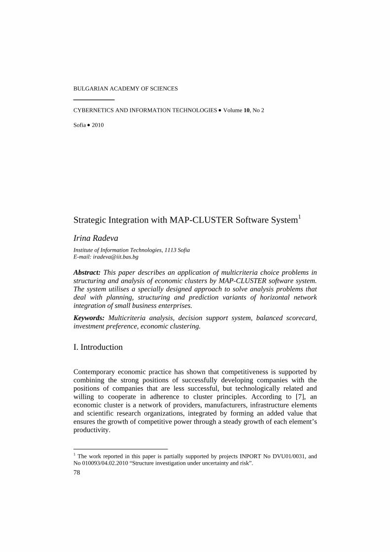
The system includes stages, which are structured in three functional blocks (A, B, C), each one comprised of certain steps. Fig. 1 shows a basic diagram of the system.

80

Techno. MAP

Enterprise data

Enterprise IP assessment

BSC

ECSampling

Strategic activities planning

Strategic Budgeting

EC IP assessment

EC selection

ECApproval

no yesEC 

budgetapproval

yes

no

A B C

A

Fig. 1. MAP-CLUSTER functional scheme

Block A facilitates the input of data on SBE, calculating Investment Preference evaluation criteria and calculating the values on indices, part of the integrated BSC.

It is necessary, however, that the DM takes some preliminary steps. First, the DM should have worked out a preliminary vision for the structure of the Technological Map (TM) of the EC and second, to sample the list of potential SBE candidates for integration. The TM is a horizontal network structure that links providers, manufacturers, dealers, financial institutions, scientific groups and other potential participants in the design work, manufacture and realization of a product or service, targets of the structural integration. TM consists of junctions that define the activity of different enterprises (SBE) in the production of the chosen multitude of products/services. Each junction corresponds to a number of SBE (existing or potential).

The list of thirty-two prime parameters, integrated in the system, can be found on Fig. 2. The qualitative parameters are evaluated on a five-level grading scale. The quantitative parameter data is taken from the financial reports of SBE and from national statistical data.

The prime parameters evaluated by the DM are used to calculate eleven secondary parameters, the formulae to which are shown on Fig. 3. These eleven parameters are used for estimation of a complex-valued measure of investment preference IPSBEi for each SBE.

81

Prime parameters ci Value type Prime parameters ci Value type

Technology level Index c1 qualitative Annual training costs c16 quantitative Environmental Index c2 qualitative Average sector productivity c17 quantitative Investment policy Index c3 qualitative Average wage in industry c18 quantitative Strategic policy index c4 qualitative Scientific and technological institutions

intercommunication c19 qualitative

Financial resources provision c5

qualitative Level of technological development c20 qualitative

Welfare expenditure c6 qualitative Internet procurement c21 qualitative Marketing policy c7 qualitative E-commerce c22 qualitative Database organization and management c8

qualitative Technological innovations c23 quantitative

Training c9 qualitative ISO c24 quantitative Internationalization Index c10 qualitative Market researches c25 qualitative Index of financial stability c11 qualitative Main production market share c26 quantitative Commodity composition elasticity Index c12

qualitative Strategic flexibility c27 qualitative

Annual expenditures c13 qualitative Range of products of commodities c28 qualitative Annual investment outlay c14 quantitative Average annual wage c30 quantitative Number of employees c15 quantitative Operating income c31 quantitative Information security c32 qualitative

Fig. 2. Prime parameters list

Secondary parameters Formula

D1 - Growing conditions Index (GCI) ∑

=

=9

31

iiicwD

D2 - Innovative activity Index (IAI) 13142 / ccD = D3 - Investments in human recourses (IHR)

∑=

=9

73

iii DwD ; ∑

=

=>3

1

1,0i

iww

D4 - Business - utilities (BU) 3232222114 cwcwcwD ++= ;

∑=

=>3

1

1,0i

iww

D5 - Technological and managerial innovation activity TMIA

( ) 1324235 / cccD +=

D6 - Competitive activity (CA) ∑

=

=28

256

iiicwD

D7 - Trading costs Index (TCI) 13167 / ccD =

D8 - Per person Annual average wage Index (PPAAWI)

1815308 / cccD ×=

D9 - Per person productivity Index (PPPI) 1715319 / cccD ×=

D10 - Economic creativity (EC) 207196

6

5

4

210 CaCaDqDwD

jjj

iii +++= ∑∑

==

D11 - Growth trough competitiveness (GC) ∑∑==

++=12

101

2

111

iii

iii DcqcwD

Fig. 3. Secondary parameters list

The choice of SBE is made according to a ranking by IPSBEi values, the calculation of which is presented later.

The third component of block A contains the BSC indices. This is a tool, by which a development strategy for the EC is formulated. The goals and indices of the system are determined by the defined strategic development themes and encompass four directions: finances, markets, internal business processes, knowledge and

82

development. The strategic themes indices included in MAP-CLUSTER are as follows:

Financial indices: Value of assets; Value of assets/number of employees; Revenue/Value of assets; Revenue/number of employees; Profit/value of assets; Profit/number of employees.

Markets: Number of regular clients; Number of regular suppliers; Market share; Client loyalty index; Supplier loyalty index; Reputation.

Internal business processes: Supply rhythm; Sales rhythm and time; Direct customer contacts (direct sales quota/indirect sales); Deficit of deliveries; Productivity growth; Nomenclature expansion.

Knowledge and development: Qualification expense/total expense; highly qualified specialists/all employees; scientific research expense/total expense; administration/all employees.

The structure of BSC is shown on Fig. 8. The BSC estimates are used in the third block of the system.

The second block (B) includes an estimate of IPSBEi, forming and approving EC variants, for which the strategic planning session is continued.

The complex value IPSIG is calculated by the following formulae:

( ) ( )

( ) ( )[ ]( ) ( )[ ] ,5/minmax

,5/minmax

,minmin

IP

111111

101010

11

1111

10

1010SBE

DDDDDD

DDD

DDD ii

i

−=Δ−=Δ

⎥⎦

⎤⎢⎣

⎡Δ−

×⎥⎦

⎤⎢⎣

⎡Δ−

=

where: i is an indicator of SBE, D10 is the Index of economic creativity

;...

,43

3

721

282726257

13

24236

3222215

2041931715

31

1815

30

13

16

2

13

14110

www

ccccwc

ccwcccw

cwcwccc

ccc

cc

wccwD

===

⎟⎠⎞

⎜⎝⎛ +++

+⎟⎟⎠

⎞⎜⎜⎝

⎛ ++⎟

⎠⎞

⎜⎝⎛ ++

+

+++

⎟⎟⎟⎟

⎠

⎞

⎜⎜⎜⎜

⎝

⎛ +++⎟⎟

⎠

⎞⎜⎜⎝

⎛=

D11 is the Index of growth through competitive power

.... , 1221

12

111 wwwcwD

iii ====∑

=

The value of IPSBEi ∈ [0, 25]. This estimate characterizes the order of individual SBE. It is meant to help the DM in his choice whether or not to include a particular SBE in a variant of an EC. The DM alone chooses the boundary value of IPSBEi, which will serve him as an EC inclusion criteria. The number of variants formed depends on the DM. The system only allows the inclusion of input SBE in

83

an EC. If the DM deems the values of the IPSBEi estimate for one or more SBE of a certain technological group as unsatisfactory, they can form a new EC variant with an incomplete technological network, but it must be noted during the following prognostic stages, that the missing activity in the technological group is to be compensated for either by outsourcing or by setting up a new group. The alternative EC structure variants can be as follows:

First. The TM has empty groups and they shall be serviced by means of outsourcing.

Second. The TM has empty groups and they shall be filled by newly created elements of the grouping (investments). During the prognostic period the activity shall be taken over by an element external to the network.

Third. All TM groups are full. Fourth. The TM has empty groups and they shall be filled by remediation of

elements (investments) that have been rejected during initial analysis.

The process is depicted in a diagram on Fig. 4. A TM has been entered in block (A) comprised of n groups and SBE with identifiers corresponding respectively to the belonging to the technological groups of the network and to the consecutive number (1,1; 1,2; ... , 1,n; 2,1; 2,2; ..., 2,n; n,1; ...; n,n). IPSBEi have been calculated in block B. The DM defines, for example, three variants of an EC that contain four groups. According to the boundary value of IPSBEi, only one of the three variants (variant 3) has a full TM; variant 1 has an unfilled group 3, variant 2 has an unfilled group 4. With these variants, the DM continues the planning procedure in block C.

1,1 1,2 2,11,n 2,2 2,3 3,12,n 3,2 3,3 n,13,n n,n

1 2 3 …

TM

… …

1

2 4

…3

… …

1

2 4

…3

… …

1

2 4

…3

Enterprise IP assessment

ECSampling 

ESApproval

B

C

A

yes

no

Var 1 Var 2 Var 3

Fig. 4. Stage B functional scheme

Block C is where the strategic budget planning procedures for all EC variants are carried out and where the final ranking is obtained. Strategic budgets estimation includes: expert assessment of an EC activity programme by period; estimating labour expenses; asset expenses; material and other expenses; estimating realisation

84

income and income in the profit centre of the EC; generating a consolidated budget; calculating the BSC indices and producing an arrangement of the EC variants.

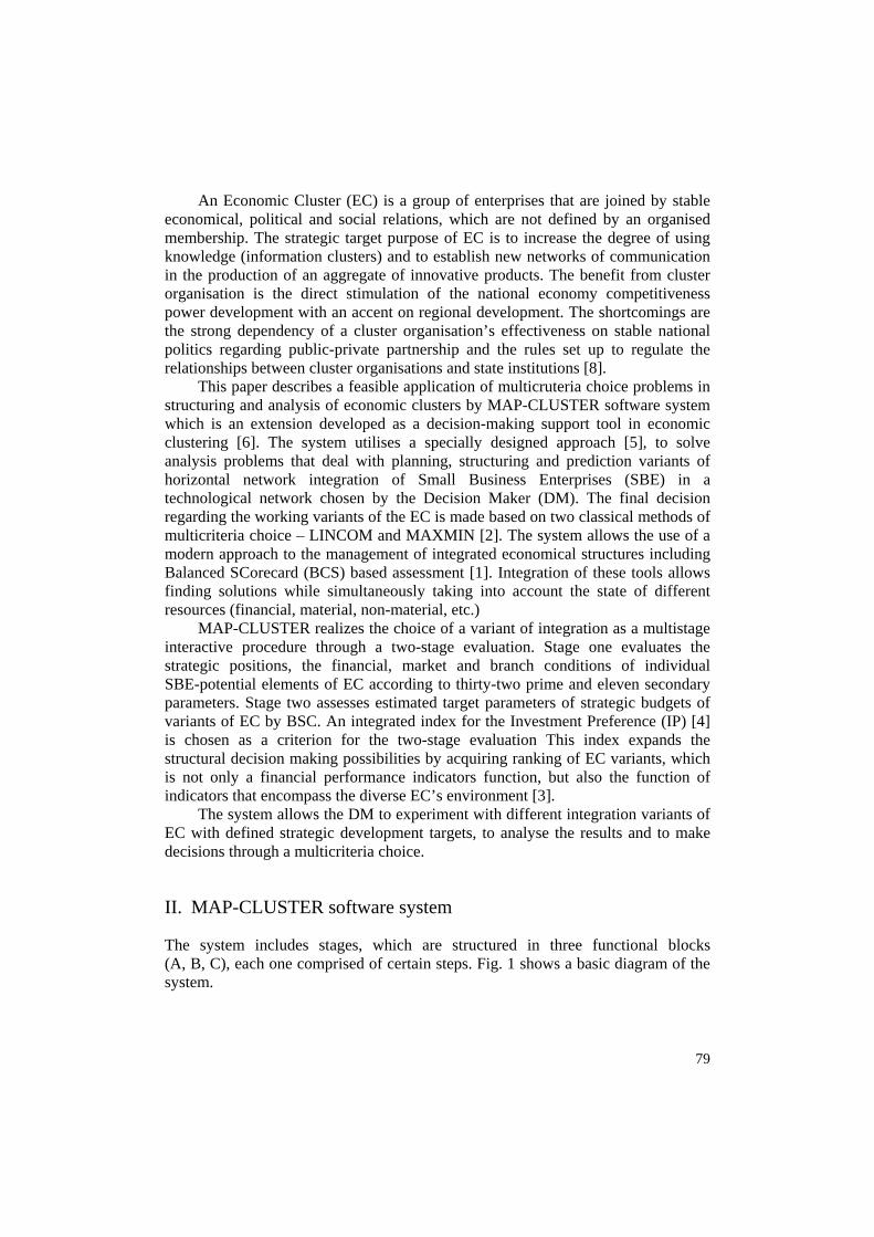
In order to form the resource expenses, the following four groups are consecutively and expertly estimated:

First group. Labour expenses for the period of planning the respective qualification groups (in kind and value), the breakdown (expertly assigned) by activity and by period. The annual labour expenses are estimated for the whole period with a change of their breakdown by activity. The qualification categories cannot be changed.

Second group. Expenses for material and non-material assets for the period of planning (in kind and value). Asset expenses are included as depreciation allowances. The breakdowns of depreciation allowances by activity are expertly assigned.

Third group. Material expenses (in kind and value), the breakdowns of these expenses by activity and period.

Fourth group. Other expenses for the planning period by type (in kind and value), the breakdowns of these expenses first by activity and then by period. When estimating the strategic budget the other expenses are not classified by item, but are expertly assigned as a total amount for the prognostic period.

The revenue of the EC is estimated for the chosen profit making centre. The revenue is formed by the income from the volume of realized production, the income from expanding the list of products, the income from international and national programmes, the income from target financing, the income from new clients (expanding the market share), loan funds (service interest is shown as “financial expenses” in the budget) and others. The value of the income and its breakdown by time can be expertly assigned.

A diagram of how revenues and expenses are formed and their breakdown by periods, quota and activities can be found in Fig. 5.

Labor costs 

Assets investments

Row mat. costs

Other expenses

n1 n2 n3 n4 n5

Expenses distribution planning

Expenses %  distribution planning

Activities distribution planning overtime horizon

Human resources Labor costs distribution 

Assets amortization distr.Assets procurement

Row mat. costs distrib.

Other expenses distrib.

Total expenses distribution overtime horizon

Total revenues distribution over time horizon in the

profit center

Revenues distributionplanning over time

horizon

Commodity composition of outputs

Volume increase 

Range  increase 

Customers  increase National and international programs fundingTarget fundingBorrowingsOthers

Row mat. procur.

C I

Fig. 5. Expenses and revenues planning scheme

85

The software system automatically generates consolidated budgets for all EC variants. The financial expenses are expertly estimated. The diagram of calculating and approving the consolidated budget can be found in Fig. 6.

Total expenses distribution overtime horizon

Total revenues distribution over 

timehorizon

Net profit

Total expenses 

Amortization expenses

Commodity output cost 

Taxes

Operating expenses 

Interests

Total revenues in the profit center

Rate ofdiscounting

Consolidatedbudget

Discounted profit

Present value cash flows (PVCFs)

++

‐

Profit 

‐X

Tax rateX

Cash flow+

X

PVCFs > 0 yes

no

III

IV

C II

Fig. 6. EC consolidated budget approval

The development, analysis and approval of the budget is a multistage interactive procedure that allows the comparison between the effects of the activity of the cluster and the resource necessities. During the process of analysis the following conditions must be observed:

First condition. The present value of cash flows PVCF > 0. The budget is considered acceptable and takes part in the procedure of choosing an EC variant.

Second condition. PVCF < 0. The estimation procedure returns to either the stage of revising the planned activities by period or the stage of estimating the costs. The iterations repeat until PVCF > 0.

The consolidated budgets of the EC variants are evaluated by the integrated BSC system. The choice of indices in the system has been made at an initial stage of the development of MAP-CLUSTER and is described in [9]. The BSC diagram is shown in Fig. 8.

86

Mission and vision

Focus of attention

Strategicobjectives

Critical successfactors

Key indicators

Investment preference criteria

Finance MarketInternal

businessprocesses

description

c5, c6, c9, c11, c13, c14, c18, c30, c2, c31

c5, c6, c9,c13, c18

description

c7, c10, c12,c17, c21, c22,c25, c26,c28

c10, c12, c21

description

c1, c2, c3, c4,c8, c20, c23,c24, c27, c32

c1, c3, c8,c20, c24

description

c16, c19

c16, c19

BSCF1, BCSF2, BCSF3, BCSF4, BCSF5, BSCM1, BSCM2, BSCM3, BSCBP1,BSCBP2, BSCBP3, BSCBP4, BSCTD1, BSCTD2

BSC Structure

Training & develop.

.1 ,1/ <⎟⎟⎠

⎞⎜⎜⎝

⎛−=

PC

SIG

PC

SIGMIP I

EIEEC .1 , IP

PC

IPIPIPPCIP C

ICCCIC −=

Δ=−=Δ ϑ

C III

Fig. 7. Strategic budget BSC validation

A critical point of investment preference (CIP) is calculated for the consolidated strategic budgets. It is an indicator of the cross point between the changes in the cumulative expenses for the activity of the EC and the changes in the income of the activity generated by these expenses. It is calculated by the following formula:

,1 ,1 PC

SIG

PC

SIG

MIP <

⎟⎟⎠

⎞⎜⎜⎝

⎛−

=IE

IE

EC

where: EM is the production expenses by cost; ESIG is the expenses for building the cluster; IPC is the income of realisation in the profit centre. The criteria for evaluating the quality of the budget are: the deviation from CIP

(∆CIP ) and θ CIP , where:

. ,PC

IPIPIPPCIP I

CCCIC Δ=−=Δ ϑ

The remaining criteria for evaluation and the method of calculation are shown in Fig. 8.

87

BSC Investment preference criteria

Financial strategic objectivesBSCF1 = Profit/ total number of employees

BSCF2 = Net profit / total expenses

BSCF3 = Net profit / total number of employees

BSCF4 = θCIP BSCF5 = Net present value / SIG construction expenses

Market strategic objectives

BSCM1 = Revenues of total of outputs/ total revenues

BSCM2 = Revenues of Range of products commodities / total revenues

BSCM3 = Revenues of new customers / total revenues

Internal business processes objectives

BSCIBP1 = License and patent purchase / total expenses

BSCIBP2 = SIG construction expenses / total expenses

BSCIBP3 = Information system development / assets expenses

BSCIBP4 = Total Management expenses / assets expenses

Training and development strategic objectives

BSCTD1 = Number of highly qualified specialists/ total number of employees

BSCTD2 = Investments in human recourses/ total expenses

Fig. 8. BSC investment preference criteria

To get a final ranking of the EC variants, the DM inputs a weight ratio for all criteria included in the BSC. The sum total of the weight ratios must equal 1. The system uses two methods of multicriteria choice – LINCOM and MAXIMIN (Fig. 9).

BSC Investment preference assessment

BSCF1 BSCF2 BSCF3 BSCF4 BSCF5

BSCM1 BSCM2 BSCM3

BSCBP1 BSCBP2 BSCBP3 BSCBP4

BSCTD1 BSCTD2

C IV

Criteriawaits

Input Σ=1C III

LINCOM

MAXIMIN

Fig. 9. BSC criteria weights input

III. Investment preference assessment problem

Let us view the following problem: choose an EC variant with a horizontal technological network, comprised of five groups: centre, supplier, trader, manufacturer, other. Analyze 12 SBE. Form at least two EC variants.

88

For shortness of presentation, the expert assessment of prime and secondary criteria are not presented here. The order of SBE by IPSBEi values is presented in Fig. 10.

Technology map unit Enterprise ID IPSBE value

Center

SBE12 25.0

SBE1 0.2

SBE2 0.1

Supplier

SBE4 0.2

SBE3 0.1

Trader

SBE10 4.4

SBE11 0.5

Manufacturer

SBE9 9.2

SBE8 1.1

SBE5 0.1

SBE6 0.1

Other

SBE4 5.4

Fig. 10. IPSIG values

The results do not allow forming an EC with a complete TM. Based on the evaluations, three variants are formed on equal incomplete TM: Centre, Manufacturer, and Trader. The variants are shown in Fig. 11.

12 1 4 5 10 11

1 2 3

2 6 8

4

93

5

7

1 – Center2 – Supplier3 – Trader4 – Manufacturer 5 – Other

12/25

9/9.2

10/4.4

1

4

3

12/25 10/4.4

1

4

3

8/1.1

11/0.3

Var 312/25

9/9.2

11/0.3

1

4

3

8/1.1

Var 2

Var 1

Fig. 11. EC Sampling

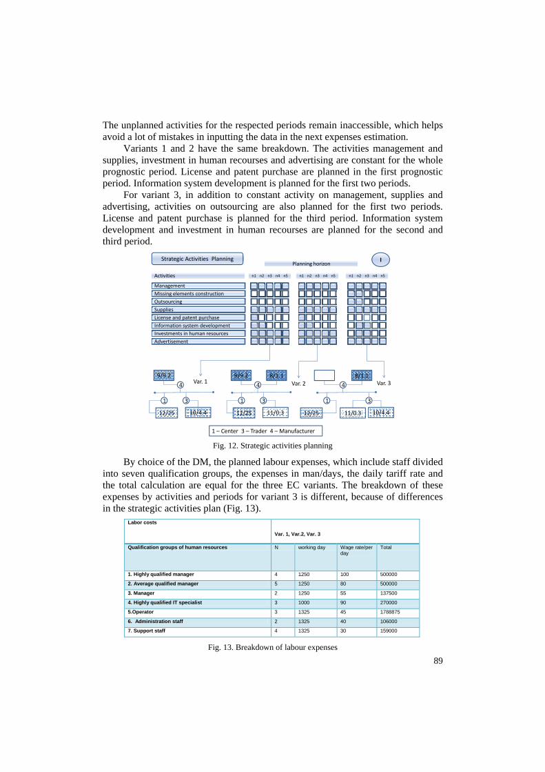
The DM plans a breakdown of activities by periods (Fig. 12). The filled squares show that expenses are planned for the particular activity and period. The unfilled squares indicate a lack of planned expenses for these activities and periods.

89

The unplanned activities for the respected periods remain inaccessible, which helps avoid a lot of mistakes in inputting the data in the next expenses estimation.

Variants 1 and 2 have the same breakdown. The activities management and supplies, investment in human recourses and advertising are constant for the whole prognostic period. License and patent purchase are planned in the first prognostic period. Information system development is planned for the first two periods.

For variant 3, in addition to constant activity on management, supplies and advertising, activities on outsourcing are also planned for the first two periods. License and patent purchase is planned for the third period. Information system development and investment in human recourses are planned for the second and third period.

1 – Center  3 – Trader  4 – Manufacturer

12/25

9/9.2

10/4.4

1

4

3

12/25 10/4.4

1

4

3

8/1.1

11/0.3

Var. 3

12/25

9/9.2

11/0.3

1

4

3

8/1.1Var. 2Var. 1

Management Missing elements constructionOutsourcingSuppliesLicense and patent purchase Information system developmentInvestments in human resourcesAdvertisement 

n1 n2 n3 n4 n5Activities n1 n2 n3 n4 n5 n1 n2 n3 n4 n5

Strategic Activities  PlanningPlanning horizon

I

Fig. 12. Strategic activities planning

By choice of the DM, the planned labour expenses, which include staff divided into seven qualification groups, the expenses in man/days, the daily tariff rate and the total calculation are equal for the three EC variants. The breakdown of these expenses by activities and periods for variant 3 is different, because of differences in the strategic activities plan (Fig. 13).

Labor costs Var. 1, Var.2, Var. 3

Qualification groups of human resources N working day Wage rate/per day

Total

1. Highly qualified manager 4 1250 100 500000

2. Average qualified manager 5 1250 80 500000

3. Manager 2 1250 55 137500

4. Highly qualified IT specialist 3 1000 90 270000

5.Operator 3 1325 45 1788875

6. Administration staff 2 1325 40 106000

7. Support staff 4 1325 30 159000

Fig. 13. Breakdown of labour expenses

90

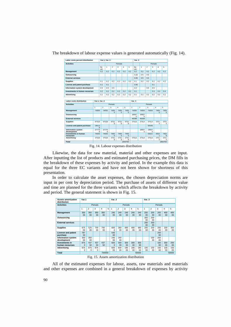
The breakdown of labour expense values is generated automatically (Fig. 14). Labor costs percent distribution Var.1, Var. 2 Var. 3

Activities Periods Periods

By act.

1 2 3 4 5 By act.

1 2 3 4 5

Management 0.2 0.2 0.2 0.2 0.2 0.2 0.2 0.2 0.2 0.2 0.2 0.2

Outsourcing 0.20 0.5 0.5

External services 0.05 0.5 0.5

Supplies 0.1 0.2 0.2 0.2 0.2 0.2 0.1 0.2 0.2 0.2 0.2 0.2

License and patent purchase 0.1 0.1 0.05 0.1

Information system development 0.3 0.5 0.5 0.2 0.5 0.5

Investments in human recourses 0.2 0.2 0.2 0.2 0.2 0.2 0.1 0.3 0.3 0.4

Advertising 0.1 0.2 0.2 0.2 0.2 0.2 0.1 0.2 0.2 0.2 0.2 0.2

Labor costs distribution Var.1, Var. 2 Var. 3

Activities Periods Periods

1 2 3 4 5 1 2 3 4 5

Management 74055 74055 74055

74055

74055

74055 74055 74055 74055

74055

Outsourcing 185070

185070

External services 46268 46268

Supplies 87028 87028 87028

87028

87028

37014 37014 37014 37014

37014

License and patent purchase 185138

92535

Information system development

277708

277708

185070

185070

Investments in human recourses

74055 74055 74055

74055

74055

55521 55521

74028

Advertising 37028 37028 37028

37028

37028

37014 37014 37014 37014

37014

Total 1850700 1850700 Fig. 14. Labour expenses distribution

Likewise, the data for raw material, material and other expenses are input. After inputting the list of products and estimated purchasing prices, the DM fills in the breakdown of these expenses by activity and period. In the example this data is equal for the three EC variants and have not been shown for shortness of this presentation.

In order to calculate the asset expenses, the chosen depreciation norms are input in per cent by depreciation period. The purchase of assets of different value and time are planned for the three variants which affects the breakdown by activity and period. The general statement is shown in Fig. 15.

Assets amortization distribution

Var.1 Var. 2 Var. 3

Activities Periods Periods Periods

1 2 3 4 5 1 2 3 4 5 1 2 3 4 5

Management 35000

35000

35000

35000

24000

24000

24000

24000

24000

20000

20000

20000

40000

40000

Outsourcing 30000

20000

External services 20000

20000

Supplies 87500

52500

70000

70000

6000

36000

48000

48000

48000

20000

20000

20000

20000

30000

License and patent purchase

78750

54000

20000

Information system development

35000

35000

24000

24000

10000

20000

Investments in human recourses

8750

43750

43750

43750

6000

30000

30000

30000

30000

10000

30000

20000

Advertising 8750

8750

8750

60000

60000

18000

18000

18000

10000

10000

10000

10000

10000

Total 700000 60000 50000 Fig. 15. Assets amortization distribution

All of the estimated expenses for labour, assets, raw materials and materials and other expenses are combined in a general breakdown of expenses by activity

91

and period. For comparison the total estimated expenses for the three EC variants are presented in Fig. 16.

The revenue of the EC is estimated for the chosen profit making centre. The revenue is formed by the income from the volume of realized production, the income from expanding the list of products, the income from international and national programmes, the income from target financing, the income from new clients (expanding the market share), loan funds (service interest is shown as “financial expenses” in the budget) and others. The value of income and its breakdown by time can be expertly assigned. The generalised data on the planned revenue for the three EC variants is presented in Fig. 16. The values for each position of revenues and expenses in Fig. 16 are shown with accrual for the whole prognostic period. This is true for all following statements.

Total revenues Var. 1 Var. 2 Var. 3

Volume of output increase 89500000 183500000 127100000 Range of products commodities increase 15000000 7000000 15000000

Customers increase 430000 840000 420000 National and international programs funding 100000 100000 100000

Target funding 0 0 0 Borrowings 250000 250000 250000

Others 0 0 0

Total 99280000 191690000 136870000

Total expenses Var. 1 Var. 2 Var. 3

Activities

Management 905275 890000 705140

Outsourcing 1392640

External services 1105036

Supplies 116390 1153500 682570

License and patent purchase 1038888 1016500 892535

Information system development 1405412 1390500 597640

Investments in human recourses 1290275 1281000 442570

Advertising 645140 643500 432570

Total 6451380 6375000 6250701

Fig. 16. Total expenses for EC variants

The consolidated budget is prepared for each EC variant. The diagram for calculating the consolidated budget is shown in Fig. 8. With the so planned revenues and expenses, the present value of cash flows is positive for all periods of planning. This makes the planned strategic budgets acceptable. The results for the consolidated budgets are shown in Fig. 17.

Consolidated budget Var. 1 Var. 2 Var. 3

Profit center total revenues 99280000 191690000 136870000 Operating expenses 6451380 6375000 6250701

Commodity output cost 20750000 45750000 25550000 Interest expenses 50000 50000 50000

Amortizations 700000 600000 500000 Total expenses 27951380 52725000 32300700

Profit 71328620 138965000 104569300

Net profit 7232863 13896500 10456930

Taxes 64195750 125068500 94112370

Rate of discounting 6% 6% 6%

Discounted profit 110864500 218896300 157767400

Cash flows 64895750 125668500 94612370

Present value of cash flows 59202140 117175100 82477430

Fig. 17. Consolidated budgets for EC variants

92

The calculated values of BSC criteria are shown in Fig. 18.

Investment preference criteria values Var. 1 Var. 2 Var. 3 Criteria waits

Financial strategic objectivesBSCF1 8334348 4316522 5950870 0.3

BSCF2 2.3721 2.2967 2.9136 0.015

BSCF3 5437761 2791120 4091842 0.015

BSCF4 0.2469 0.2235 0.1956 0.015

BSCF5 19.7127 10.0592 15.1363 0.015

Market strategic objectives

BSCM1 0.9573 0.9015 0.9286 0.15

BSCM2 0.0365 0.1511 0.1096 0.15

BSCM3 0.0044 0.0043 0.0031 0.1

Internal business processes strategic objectives

BSCIBP1 0.0193 0.0372 0.0276 0.01

BSCIBP2 0.1209 0.2308 0.1935 0.01

BSCIBP3 2.3175 2.0077 1.1953 0.01

BSCIBP4 1.4833 1.2982 1.4103 0.015

Training and development strategic objectives

BSCTD1 0.1739 0.1789 0.1739 0.01

BSCTD2 0.0243 0.04612 0.0137 0.185

Fig. 18. IP criteria values

After inputting weight ratios for each criterion, the final ranking of the EC variants can be seen in Fig. 19.

EC Variant Comment Assessment

LICOM

Var. 1 Completed TM 0.820

Var. 2 Completed TM 0.789

Var. 3 Uncompleted TM 0.686

MAXIMIN

Var. 1 Completed TM 0.363

Var. 3 Uncompleted TM 0.242

Var. 2 Completed TM 0.205

Fig. 19. EC variants ranking

The final result shows: according to the two methods the most preferable EC variant is the first one. With the weights of the criteria distributed this way by the DM, he/she shows main preference towards financial performance and more specifically – towards the index BSCF1, that calculates the accumulated profit per number of employees. As a whole this variant has the most compact structure. The second and third variants switch places in the second order due to the fact that the minimum guaranteed result, the main index of which is BSCF4, has the lowest value in variant 3. This variant also foresees outsourcing because the DM defines the TM as incomplete.

93

IV. Conclusion

The proposed approach of multicriteria evaluation of IP of the EC according to BSC allows the assessment of the quality of functioning of an integrated system while taking into account different aspects of its activity like structure, planning and management. The decision is made through an interactive problem of multicriteria choice. Due to the fact that some of the parameters are unspecified and they are often determined by expert procedures, seeking solution through algorithms of multicriteria choice provides an objective decision with the accuracy necessary for applied problems. The approach allows the integrated system of balanced scorecard to ensure balance between short-term and long-term goals, financial and non-financial indicators, internal and external factors of the activity.

Contemporary tendencies of restructuring the economy in times of financial crisis and the actuality of problems in the integral grouping of small and medium enterprises with the purpose of lessening the negative effects and providing conditions for growth, demand the development of adequate and adaptive tools to aid the process of decision making. For future development of the proposed approach and the MAP-CLUSTER system we can point out the use of other methods of multicriteria evaluation and optimization as well.

R e f e r e n c e s

1 . K a p l a n, R. The Balanced Scorecard: Translating Strategy into Action. Harvard Business School Press, 1996.

2 . P o p c h e v, I. A Technology for Multicriteria Assesment in Decision Making. – Journal of Bulgarian Academy of Sciencies, 5 (XXXII), 1986.

3 . P o p c h e v, I., I. R a d e v a. An Investment Preference under Incomplete Data. – DECOM-TT IFAC 2004, 243-248.

4 . P o p c h e v, I., I. R a d e v a. A Decision Support Method for Investment Preference Evaluation. – Cybernetics and Information Technologies, Vol. 55, 2006, 3-16.

5 . P o p c h e v, I., I. R a d e v a. MAP-CLUSTER: An Approach for Latent Cluster Identification. – In: IFAC CEFIS 2007: Synergy of Computational Economics and Financial and Industrial Systems, Istanbul, November 2007, 63-67.

6 . P o p c h e v, I., I. R a d e v a. Multi Criteria Scheme for MAP-Cluster Indentification. – Problems of Engineering Cybernetics and Robotics, 58, 2007, 3-12.

7 . P o r t e r, M. On Competition, Clusters and Competition: New Agendas for Companies, Governments, and Institutions. Boston, Harvard Business School Press, 1998.

8 . R a d e v a, I., T. N a n e v a. Economic Clusters Identification. – Automatics and Informatics, 4, 2007 (in Bulgarian).

9 . R a d e v a, I. Balance Score Card Application in Investment Preference Multi-Criteria Evaluation. – In: Proc. of Conference “Corporate Finance in Bulgaria: Today and Tomorrow”, 2009 (in print, in Bulgarian).