Strategic Trade Policy in International Trade:

To what extent did Airbus’ entry into the market for aircraft change welfare

around the world?

Bachelor Thesis by Sjors van Kuik (10274855)

June 2014

Supervised by R. Teulings

ABSTRACT

This paper aims at reviewing the validity of the Brander-Spencer model (1985) and finding out

whether it holds in the Airbus-Boeing dilemma in particular. The Brander-Spencer model states that

under certain restrictive assumptions, subsidies to home firms can increase domestic welfare,

decrease foreign welfare and increase global welfare. The model is criticized due to uncertainties

policy makers face, the fact that promoting one industry could put other industries at a disadvantage

and because possible new entrants could prevent excess profits to exist in the specific market. Since

we do not know exactly what the market situation would be when Airbus had not entered, while this

is of importance to estimate the welfare effects due to Airbus’ entry, authors consider multiple

scenarios for comparison. These welfare effects seem to be ambiguous for Europe, indicating that

the Brander-Spencer model did not hold in this case. Moreover, welfare effects seem to be negative

for the US and positive for the rest of the world. Authors are careful with making statements because

outcomes depend crucially on certain parameters used in their models. Overall, this strategic trade

policy seems to have had a negative effect on the world’s welfare.

TABLE OF CONTENTS

Section I: Introduction…………………………………………………………………………………………………….….. 4

Section II: The Brander-Spencer model………………………………………………………………………….….. 6

Section II-B: Criticism concerning the Brander-Spencer model…………………………….... 10

Section III: Empirical testing of the Brander-Spencer model……………………………………………….. 11

Section III-B: Commuter aircraft……………………………………………………………………………... 11

Section III-C: Empirical evidence in various industries…………………………………………….. 14

Section IV: Airbus-Boeing dilemma……………………………………………………………………………………… 15

Section IV-B: Wide bodied jet aircraft……………………………………………………………………… 15

Section IV-C: Entry into the market for large transport aircraft…………………………...... 21

Section IV-D: Adding a third producer………………………………………………………………....…. 26

Section V: Conclusions……………………………… ………………………………………………………………….….... 28

Section VI: Discussion………………………………………………………………………………………………….…...... 29

References…………………………………………………………………………………………………………………….…….. 31

4

Section I: Introduction

Carbaugh and Olienyk (2001) explain that the aerospace industry, which consists of space, defence

and commercial aircraft, is thought of as an important creator of wealth and employment. For this

reason and many others, like prestige and national defence, Europe and the United States compete

severely in this industry.

While before World War II there were only small aircraft producers who produced a limited

amount of jets, during the war military aircraft were produced in big quantities. After the war,

aircraft suppliers used their obtained experience and advanced technology to produce commercial

jets instead, which required similar technologies. The USA quickly became dominant in this market,

using its huge experience in building military aircraft. The aircraft industry transformed into an

industry with high research and development (R&D) costs, but strong economies of scale due to its

steep learning curve (research discussed later on by Baldwin & Krugman (1988), Klepper (1990) and

Neven et al. (1995) all assume a learning elasticity with an absolute value of 0.2, which means that

when firms double their amount of aircraft produced, marginal costs will decrease by as much as

20%). As an industry with such economies of scale is not efficient with many small producers, firms

found themselves better off merging with competitors to create synergy (profits of the merger

exceeds the sum of individual profits). This development heavily reduced the number of firms in the

industry. During the 1970s there were only three American aircraft producers left, dominating the

world market: Boeing, Lockheed and McDonnell-Douglas. Of these three, Carbaugh and Olienyk

(2001) state that Boeing was the largest, maintaining a market share of over 60%. Due to competitive

pressures, Lockheed left the market for commercial aircraft in 1971 and McDonnell-Douglas (MDD)

would merge with Boeing by 1997.

European firms did not have enough output to benefit from the economies of scale this

industry offers, nor did they have governments spending amounts comparable to the USA on military

aircraft. Carbaugh and Olienyk (2001) say that Europe could not accept the fact that their presence

(and profits) in this industry would be completely zero. Therefore, in 1970, they brought Airbus into

the market for commercial aircraft by giving direct subsidies, which according to Europe would be

paid back once Airbus was able to do so. According to Neven et al. (1995), Europe’s motive for

introducing Airbus could also be to increase world’s consumer surplus. The increase in competition

would lower world prices, which would lead to higher levels of consumer surplus. Carbaugh and

Olienyk (2001) say that the entry of Airbus gave rise to a political debate that went on for decades,

because the USA claims that direct subsidies are unfair competition and diminished their welfare due

to lower profits.

5

Standard trade theory, as summarized by Krugman et al. (2012), states that when the home

country imposes an import tariff on a good, making its imports more expensive, the domestic price

for this particular good will also rise. The domestic price rises, because home producers, competing

against the imports, can increase their price with the size of the tariff without changing their

competitive position. This domestic price increase results in a loss in consumer surplus, a gain in

producer surplus and positive revenues for the government. When combining these effects, the total

change in welfare is negative. However, when a country is large enough, its lower quantity of imports

due to the higher price could depress the world price. When the world price of the import good

diminishes, the terms-of-trade (price of the export good divided by price of the import good)

increase. This positive welfare effect adds to the previous mentioned negative effect, making the

total change in welfare unclear. When the home country offers an export subsidy, domestic

producers have an incentive to sell abroad rather than domestically. To omit this incentive, the

domestic price must rise by the size of the subsidy. Because of this domestic price increase,

consumer surplus again decreases and producer surplus increases, only now the government has

extra costs instead of revenues. The combined effect again is a negative one. When the country

imposing the subsidy is large, increased world supply will decrease the world price for the export

good, deteriorating the terms-of-trade so that the negative welfare effects are even more severe. It

can be concluded that import tariffs have an ambiguous effect on welfare and that welfare strictly

decreases by giving export subsidies.

In contrast to the standard trade theory, the Brander-Spencer (1985) (BS) model shows that

under certain assumptions export subsidies can actually be welfare improving. Governmental

subsidies would allow domestic firms to reap excess profits in imperfectly competitive markets.

Because these excess profits are shifted from the foreign to the domestic firm, domestic welfare

increases at the expense of the foreign country. If this model would hold in the given situation, the

EU would increase its welfare at the expense of the US’s by introducing Airbus.

A goal of this paper is to analyse the welfare effects in Europe, the US and the rest of the

world due to the entry of Airbus into the market for commercial aircraft. In section II of this paper,

the BS model with its underlying assumptions will be discussed. Criticism concerning the model will

also be addressed in this section. In the following section, empirical research on the BS model in

various industries will be covered to obtain a general idea about whether it holds in practice. In

section IV the focus will shift again to the Airbus-Boeing event, where in the three subsections

empirical research on this matter is discussed in detail. In section V possible conclusions are drawn

about the validity of the BS model and about the welfare effects concerning Airbus. The final section

will be a discussion about the validity of this research itself.

6

Section II: The Brander-Spencer model

To analyse the welfare effects due to the subsidized entry of Airbus into the Aircraft market, an

understanding of the Brander Spencer (1985) (BS) model is relevant. Therefore, a summary of the

model and the underlying assumptions will be given below. During later research, the model has

been criticized by various authors. These papers will be discussed in subsection IIB to provide

objectivity on the validity of the model.

BS notice that subsidies in international rivalry are an often practice in Western economies

and that there is a growing belief such policies are unfair. In their paper, they try to understand why

subsidies might be effective strategies. While constructing their model, BS impose the following

assumptions: first of all, the analysis is based on imperfect competition, because excess profits must

be available in the industry. Second, it requires an industry with at least two exporting countries,

exporting an identical good to a third country. In the third place, BS use the Cournot duopoly model

as their equilibrium model. The model can be viewed as a two-stage game, in which governments

decide their subsidy levels in the first stage and firms decide their output levels in the second stage.

Because firms decide their output levels after the subsidy level is set by the government, this

interaction is an example of Stackelberg competition in which governments are leaders and firms are

followers. Besides the subsidy level, in Cournot competition, firms also base their output on the

output levels set by their rivals. BS assume that the outcome in each stage will be at an optimal level,

being the Nash equilibrium. This implicates that governments play Nash against each other and so do

firms against each other. Finally, all produced items are exported and thus not consumed by the

exporting countries themselves.

BS explain that when their assumptions do not hold, results may not be the same. Eaton and

Grossman (1986) prove this fact by calculating that in a Bertrand duopoly, where firms compete in

prices rather than output, an export tax, instead of an export subsidy, is in fact the optimal trade

policy. An export tax decreases the level of domestic output, which decreases the total output

delivered by this duopoly. As a result, prices go up and the output level moves more towards

monopoly output, which raises domestic welfare. Eaton and Grossman also show, that when firms

exactly know what their rivals will do in terms of price and output, free trade is optimal. These results

show that the validity of the BS model is very sensitive to the underlying assumptions.

BS start their analysis by setting up a profit function for both the home firm (π) and the

foreign firm (π*):

���,�; �� = ���� + �� − ���� + �(�) (1)

7

As can be seen in the formula, the profit function for the home firm is equal to its market share (x)

times the inverse demand, which is denoted by p(x+y) (y is market share of foreign firm), minus the

total costs (c), plus the subsidy revenue (s). The foreign firm has the same profit function, only

without the subsidy revenue. Next, they take the first order condition of these functions and equalize

them to zero, since both firms are striving for maximum profit. The first order condition functions

represent the firms’ reaction curves, which represent the best choice in terms of output (remember

from the assumptions that this choice is based on output levels of rival firms and subsidy levels of

governments). For the home firm this function equals:

�� = ��� + � − �� + � = 0 (2)

In which first order conditions are denoted by subscripts, with the exception of p’, which is also a first

order condition. To represent that reaction functions are concave and decreasing, the second

derivatives are set to be smaller than zero. For the home firm these second order conditions are

shown in function (3) and (4):

��� = 2�� + ���� − ��� < 0 (3)

��� = �� + ���� < 0 (4)

Function (3) shows the changes in marginal profits due to changes in own output, whereas function

(4) does the same for changes in foreign output. BS assume that the former effect dominates the

latter:

��� < ��� (5)

Because function (5) is not only true for the home firm, but also for the foreign firm, BS are able to

state that D is larger than zero. D is not a variable, but is arbitrarily chosen for referring purposes:

= ������∗ − ������

∗ > 0 (6)

To find the effect of the subsidy (s) on market shares (x and y), the total derivative of the first order

conditions is set equal to zero. The total derivative means differentiating the reaction function with

respect to x, plus with respect to y, plus with respect to s. πxs and π*ys of this total differentiation

are known, because they are one and zero respectively (where one represents a subsidy and zero

8

does not). The remaining part of the formula can be solved by converting to a matrix form and

solving with Cramer’s rule. BS find:

�� � ��/�� � ����∗ /� 0 (7)

�� � ��/�� � ���∗ /� 0 (8)

These functions show the effect of the subsidy imposed by the home country on market shares. It

can be noticed that the subsidy has a positive effect on its own market share (7), but lowers the

market share of the foreign firm (8). Note that the fact that the positive D, that was defined above, is

used here to indicate the direction of the inequality symbol.

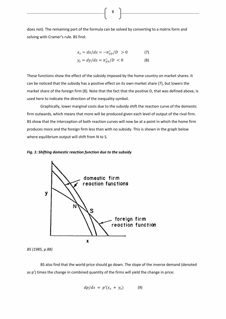
Graphically, lower marginal costs due to the subsidy shift the reaction curve of the domestic

firm outwards, which means that more will be produced given each level of output of the rival firm.

BS show that the interception of both reaction curves will now be at a point in which the home firm

produces more and the foreign firm less than with no subsidy. This is shown in the graph below

where equilibrium output will shift from N to S.

Fig. 1: Shifting domestic reaction function due to the subsidy

BS (1985, p.88)

BS also find that the world price should go down. The slope of the inverse demand (denoted

as p’) times the change in combined quantity of the firms will yield the change in price:

��/�� � �’��� ���� (9)

9

Using the results obtained in equations (7) and (8), this function can be rewritten:

�/� = �’(���∗ − ���

∗ )/ < 0 (10)

From function (5), it must hold that the part between brackets is positive. Since D was defined as a

positive number and the slope of the inverse demand is strictly negative, world prices must decrease

with home’s subsidy.

Next, BS investigate the change in domestic surplus. They set up a domestic surplus function,

which equals profits minus the costs of the subsidy itself and take the first order condition of this

function with respect to the subsidy. They find that the subsidy increases domestic surplus. BS

explain that in their model for domestic surplus, the positive subsidy is added to the firm’s profit, but

the same amount is subtracted from the government, yielding a net change of zero. BS explain that

the positive effect on domestic surplus arises because the government, who acts first in this two-

stage game, is able to change the reaction curve of the home firm to a more favourable position.

Because of this fact, BS state that countries have unilateral incentives to offer subsidies. The most

favourable position for the home firm is to be the leader in Stackelberg competition, which means

that the foreign firm will only decide its output once the home firm has already done so. This makes

the home firm the market leader. BS finally find that the Nash equilibrium is at the point where both

firms offer an export subsidy and that joint welfare of home and foreign would be higher when the

subsidy levels would be lower than Nash.

BS sum up their results in their so called propositions. These are:

Proposition 1: ‘’an increase in the domestic subsidy will increase domestic profit, decrease foreign

profit and lower the world price’’ (1985, p. 87)

Proposition 2: ‘’The domestic country has a unilateral incentive to offer an export subsidy to the

domestic firm’’ (1985, p. 87)

Proposition 3: ‘’The optimal export subsidy moves the industry equilibrium to what would, in the

absence of a subsidy, be the Stackelberg leader-follower position in output space, with the domestic

firm as leader.’’ (1985, p. 89)

Proposition 4: ‘’The noncooperative Nash subsidy equilibrium is characterized

by positive production subsidies in both exporting countries.’’ (1985, p. 95)

Proposition 5: ‘’At the noncooperative Nash subsidy equilibrium joint welfare of the producing nations

would rise if subsidy levels were reduced.’’ (1985, p. 95)

10

Section II-B: Criticism concerning the Brander-Spencer model

Krugman (1987) mentions that implementing strategic trade policy is difficult because of uncertainty.

He explains that policy makers do not know the exact values of the payoff matrix (a payoff matrix

displays the payoffs of the home and foreign firm with no intervention versus the payoffs at various

subsidy levels). Because of uncertainty, such strategies carry risks: one’s own calculation could

contain an error, for example when payoffs at a certain subsidy level are calculated too

optimistically, the value of the subsidy might be higher than the obtained excess returns. In addition,

foreign policy makers could make use of wrong numbers, resulting in an unexpected action. Krugman

adds to the uncertainty argument that even when calculations are correct, policy makers do not have

full information about how oligopolies behave.

Dixit and Grossman (1986) explain that the BS-model assumes that only the industry in

question is oligopolistic, while all other industries are perfectly competitive. The general equilibrium

principle states that resources given to a particular industry must be drawn away from other

industries. When other industries are perfectly competitive, no excess returns are lost when

resources are moved out of these industries, because these excess returns are not present. However,

when other industries are not all perfectly competitive, excess returns are in fact lost by pulling

resources out of these industries, decreasing the overall effect due to the subsidy. Dixit and

Grossman argue that this problem is even more severe when several industries in a sector use a

specific common input factor. The subsidized industry will bid up the price of this factor, putting

other industries at a disadvantage. When other industries are not all perfectly competitive,

governments must not only have full information about the industry they are to promote, but must

also have information about the losses other industries will face due to this strategy. This fortifies

Krugman’s uncertainty argument.

Horstmann and Markusen (1986) argue that possible new entrants could decrease the excess

returns obtained by the subsidy (BS assume a fixed number of firms, not taking into account possible

new entrants). When new firms enter the industry, they will take (part of) the excess returns, which

were in fact the aim of the subsidy. In the case where all excess returns are taken by new entrants

and are thus not available anymore, the entire value of the subsidy will be shifted towards

consumers indirectly in the form of lower prices. Markusen and Venables (1988) say that not only a

fixed number of players versus free entry matters, but also whether international markets are

segmented or integrated. They conclude that an export subsidy increases welfare by more (or

decreases welfare by less) when markets are segmented rather than integrated. In the case that they

are segmented, a firm sets independent sales in the home country and in foreign countries, allowing

for different prices. On the other hand, when international markets are integrated, domestic and

11

foreign prices will be equal. The difference between these two is that when markets are segmented,

this policy will not affect the world price of the foreign product, where in integrated markets it would

decrease through a decrease in world price for the domestic good. This will omit the import terms of

trade effect due to an export subsidy, leading to increased welfare. BS assumed that the exporting

countries have no consumption themselves, so do not differentiate between these two market

structures.

Since an export subsidy as described by BS is assumed to raise national welfare, but decrease

foreign welfare, according to Krugman (1987) this could lead to retaliation by the foreign country. If

the foreign country retaliates by giving a subsidy too, joint surplus of home and foreign would

decrease. This can be concluded referring back to proposition 5 by BS, which stated that when home

and foreign deviate from Nash by lowering their subsidies, joint surplus would increase. Note that

this is actually the opposite. Krugman adds that increased welfare does not mean increased welfare

for everyone. He explains that when such policies indeed lead to increased welfare, it would also

cause a redistribution of income. He claims that income would most likely be shifted to small,

influential groups of people, because they will put pressure on governments only when they benefit.

Section III: empirical testing of the Brander-Spencer model

Thus far, based on the theoretical side only, we cannot tell whether the Brander Spencer model

holds in practice. For this reason, practical research is highly relevant in this matter. Most empirical

research has been conducted in the Aircraft industry. According to Baldwin and Krugman, ‘’the

Aircraft industry is a natural target for those who study the new trade theory, which emphasizes

increasing returns, dynamics and imperfect competition’’ (1988, p. 45). They also mention the great

political conflict between the United States and the European Union as an additional reason to study

this particular sector. Since the rest of this paper focuses on this conflict, the following subchapters

will be used for research on the BS model other than Airbus-Boeing. In section III-B, research on the

commuter aircraft market will be shown in detail, because this industry is closely related to the

commercial aircraft industry. In section III-C, research on the BS model is examined in various other

industries.

Section III-B: Commuter aircraft

Baldwin and Flam (1989) empirically test the Brander-Spencer model in the market for 30-40 seat

commuter aircraft. They explain that this industry is very much like the theoretical situation

described by BS and therefore makes it an excellent field for investigation: three firms, of which one

12

Canadian, one Brazilian and one Swedish control this market and produce close to homogenous

goods. This market behaves like the general aircraft market discussed in the introduction, thus has

high start-up/R&D costs, but a steep learning curve. The Brazilian and Swedish firm have almost no

consumption of their own (as assumed by BS), therefore export nearly all goods. Canada does have

own consumption, amounting to about 40% of its sales.

In considering demand, Baldwin and Flam assume that jets will sell for 20 years until a new

model is introduced. Airliners are assumed to buy a constant number of jets (x) per year and use

them to create service revenue. An important note is that these aircraft become much cheaper over

time due to the increasing stock of aircraft (marginal utility decreases), making today’s price a

function of past and future output (see figure 2). Concerning the supply side, Baldwin and Flam set

up a cost function using fixed costs and decreasing variable costs. Both the supply and demand side

are assumed to strive for maximum profits.

Baldwin and Flam calibrate their model based on values of 1987. They view the jets as

perfect substitutes and obtain a price of $6 million per plane. Based on estimations by the companies

themselves, they use an output of 1100 aircraft for the next 20 years, equalling 55 jets per year. For

the discount rate they use 5% annually and the elasticity of demand is set at 1.5 (which is somewhat

arbitrary because an official number for this particular market is not known). For R&D costs they use

$220 million which was reported for the SF 340 (the Swedish model). Using these numbers, Baldwin

and Flam calculate the learning rate, which is used to graph the marginal costs over time. They also

estimate the price-path over time. These results can be seen in figure 2 below. Note that the price

falls steeper than marginal costs, indicating that the price decreasing effect of an increasing stock

dominates the decreasing marginal costs due to learning effects. These prices and marginal costs

over time are used for calculating the variables we are interested in, being profits of the firms and

consumer surplus.

Baldwin and Flam note from the regional distribution of sales figure, that the Swedish and

Brazilian firm are having a hard time selling on Canadian grounds. They suspect Canada of having a

certain market access restriction (MAR) policy. Moreover, they find that the Brazilian firm was able to

sell for a very low price compared to the other firms, suggesting export subsidies (ES) were received

from the Brazilian government. Baldwin and Flam compare three cases, (1) no MAR, (2) no ES and (3)

no MAR + no ES with the base case, being MAR + ES. Since Baldwin and Flam do not know the exact

nature of the MAR, they use the simplest case, being that the Canadian firm offers to Canada for the

world price, just as its competitors. Since also the size of the Brazilian subsidy is not known, Baldwin

and Flam use four different subsidy sizes in their comparison. The results can be seen in figure 3.

13

Fig. 2: Price and marginal costs relation for commuter aircraft

Baldwin and Flam (1989, p. 491)

Fig. 3: Policy effects for the base case (with subsidy of 10%)

Baldwin and Flam (1989, p. 494)

Figure 3 shows that in the base case, with the MAR and the ES, Canada is a net loser in this

market. This loss will be larger when the MAR is lifted (hence column 2). Its competitors however,

who are now able to sell for reasonable prices in Canada, increase their profits. Effects on consumer

surplus, aircraft prices and output are minor when the MAR is lifted. When an export subsidy of 10%

14

of marginal costs is given to the Brazilian firm in the base case, abolishing this subsidy will decrease

Brazilians profits by $125 million and increase profits of Canada and Sweden by $66 and $58 million

respectively. It can also be noticed that the subsidy was effective in lowering prices of aircraft and

increasing both the output and the world’s consumer surplus. Together these results indicate that

the Brander-Spencer model holds in this industry.

As mentioned earlier, Baldwin and Flam tested for four different subsidy levels, being 5, 10,

15 and 20% of marginal costs. Figure 4 shows that the 10% as used above, is in fact the optimal

subsidy level for Brazil.

Fig. 4: Changes in profits under different subsidy rates

Baldwin and Flam (1989, p. 497)

Baldwin and Flam found evidence in favour of the BS model during this research. In the next

subsection, research conducted in the automotive, semiconductor, ski production and cruise ship

market is summarized to obtain a general idea about the validity of the BS model. These industries

have characteristics similar to the aircraft industry, being high R&D/fixed costs, strong economies of

scale and are often dominated by large producers.

Section III-C: Empirical evidence in various industries

Baldwin and Krugman (1986) examine Japan’s change in welfare due to restricting its imports in the

semiconductor market. Note that an import restriction differs from an export subsidy, but either has

the ability to increase exports. Baldwin and Krugman find that Japan’s import restriction succeeds in

making them more competitive both home and abroad, but also find that total effect on welfare is

negative, because the costs exceeded the revenues. Daltung et al. (1987), who empirically test the

markets for ski production and cruise ships, find that subsidies to domestic firms are welfare

increasing in the market for ski production, but they are not able to draw a uniform conclusion for

the cruise ship market. Laussel et al. (1988) examine the Europe-Japan rivalry in the automotive

market and find that for the Netherlands and France, both import tariffs and export subsidies have

negligible effects on welfare. Though for the UK, they conclude that strategic trade policies can have

15

a significant effect on welfare. The optimal policy for the UK seems to be an export subsidy, which

could raise welfare by as much as 8.5%. They also confirm the statement made by BS that when

competing firms adopt strategic trade policy at the same time, total welfare decreases. Smith (1994)

who also examines the European car market, finds that the loss in consumer surplus in most cases

outweighs the gain in producer surplus when strategic trade policies are implemented. Therefore, his

result is that the BS model does not hold.

It can be concluded that there is evidence in favour of, but also against the BS model. Based

on these results a general conclusion cannot be drawn. In the following section the focus will shift to

the Airbus-Boeing dilemma.

Section IV: Airbus-Boeing dilemma

As mentioned in the introduction, Airbus was able to enter the market for commercial aircraft

because of subsidies granted by European governments. The purpose of this section is to test

whether the BS model holds in the Airbus-Boeing case. During later years, Carbaugh and Olienyk

(2001) explain, there have been agreements on strategic trade policies between the US and Europe.

The research discussed in this section will focus entirely on the welfare effects of the initial entry by

Airbus. In the following subchapters, three papers on this item are discussed in detail.

Section IV-B: Wide-Bodied Jet Aircraft

Baldwin and Krugman (1988) set up a model that focusses on medium-range, wide-bodied aircraft.

Baldwin and Krugman explain that not all aircraft are substitutes, because they are different in both

size and range. For this reason they consider the market for medium-range, wide bodied aircraft as a

market on its own. They say the competition between the EU and the US started when Airbus

introduced its medium-range, wide bodied A300 (Airbus’ first aircraft), which was in fact a substitute

for Boeing’s 767 (which was not sold yet, but was announced). MDD and Lockheed were also active

in the wide-bodied aircraft industry in the early years of the 1970s, but left when they noticed the

market was too small and losses were made. If Airbus was not entering the market for wide-bodied

aircraft, Boeing, with its 767 for medium-range and its 747 for long-range flights, would have had a

monopoly in this market. Baldwin and Krugman mention that the main reason Airbus would not have

succeeded on its own, is that since the introduction of the A300 it took several years before large

sales were made. Also, the sales dropped again later, when Boeing’s substitute began selling.

Deliveries of the A300 and 767 are shown in figure 5.

16

At first, Baldwin and Krugman consider the situation in which Airbus enters a market where

no other firm is producing yet and thus obtains a monopoly position. They say this is not irrelevant

because until 1982 the 767 was not sold (see figure 5) and as discussed above, there was no direct

substitute. They draw a simple monopoly position where the average cost function is above the

demand function to illustrate that entry would not be profitable under any combination of price and

quantity. Figure 6 shows that when a subsidy is given so that the firm will produce, consumer surplus

is obtained. The overall effect of the positive consumer surplus and the negative government

expenses is ambiguous and therefore, so is the change in welfare for the subsidizing country. The rest

of the world however, including the USA, could profit from the consumer surplus and does not carry

the cost of establishing this gain.

Fig. 6: Impact of subsidized entry by a monopolist

Baldwin and Krugman (1988, p. 54)

Next, Baldwin and Krugman analyse the welfare effects when a duopoly is formed, because

Boeing did enter the market for wide-bodied, medium-range aircraft, regardless of Airbus’ entry.

Fig. 5: Deliveries of commercial aircraft

Economist (1985)

17

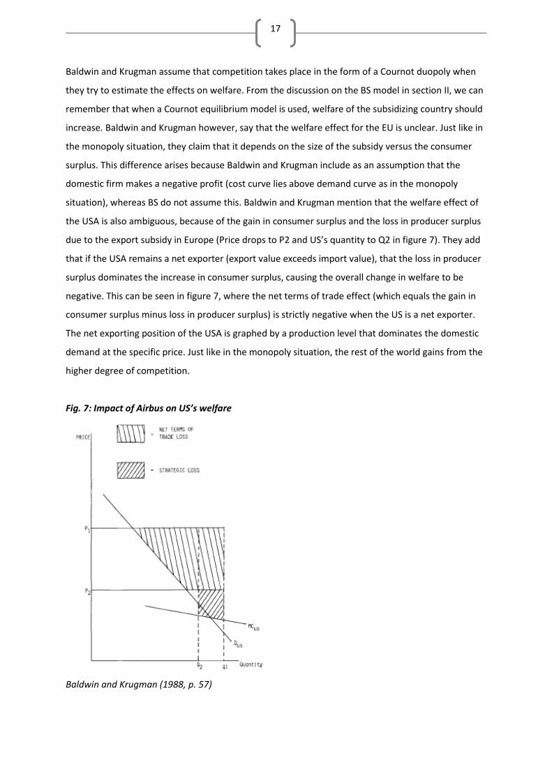
Baldwin and Krugman assume that competition takes place in the form of a Cournot duopoly when

they try to estimate the effects on welfare. From the discussion on the BS model in section II, we can

remember that when a Cournot equilibrium model is used, welfare of the subsidizing country should

increase. Baldwin and Krugman however, say that the welfare effect for the EU is unclear. Just like in

the monopoly situation, they claim that it depends on the size of the subsidy versus the consumer

surplus. This difference arises because Baldwin and Krugman include as an assumption that the

domestic firm makes a negative profit (cost curve lies above demand curve as in the monopoly

situation), whereas BS do not assume this. Baldwin and Krugman mention that the welfare effect of

the USA is also ambiguous, because of the gain in consumer surplus and the loss in producer surplus

due to the export subsidy in Europe (Price drops to P2 and US’s quantity to Q2 in figure 7). They add

that if the USA remains a net exporter (export value exceeds import value), that the loss in producer

surplus dominates the increase in consumer surplus, causing the overall change in welfare to be

negative. This can be seen in figure 7, where the net terms of trade effect (which equals the gain in

consumer surplus minus loss in producer surplus) is strictly negative when the US is a net exporter.

The net exporting position of the USA is graphed by a production level that dominates the domestic

demand at the specific price. Just like in the monopoly situation, the rest of the world gains from the

higher degree of competition.

Fig. 7: Impact of Airbus on US’s welfare

Baldwin and Krugman (1988, p. 57)

18

Since Airbus was in essence a monopolist in this specific market until the 767 started selling

in 1982, Baldwin and Krugman replicate the Airbus-Boeing dilemma by setting up a model which

captures both the monopoly and the duopoly situation respectively. As discussed above, the USA

gains in the first period and loses in the second, provided that they remain net exporters (which

Baldwin and Krugman think is a realistic assumption). The effect on the EU’s welfare would be

ambiguous in both situations. The total effect on welfare depends on the weights added to each of

the two periods. For simplification, the model is created in a world where the 767 and the A300 are

the only aircraft being produced.

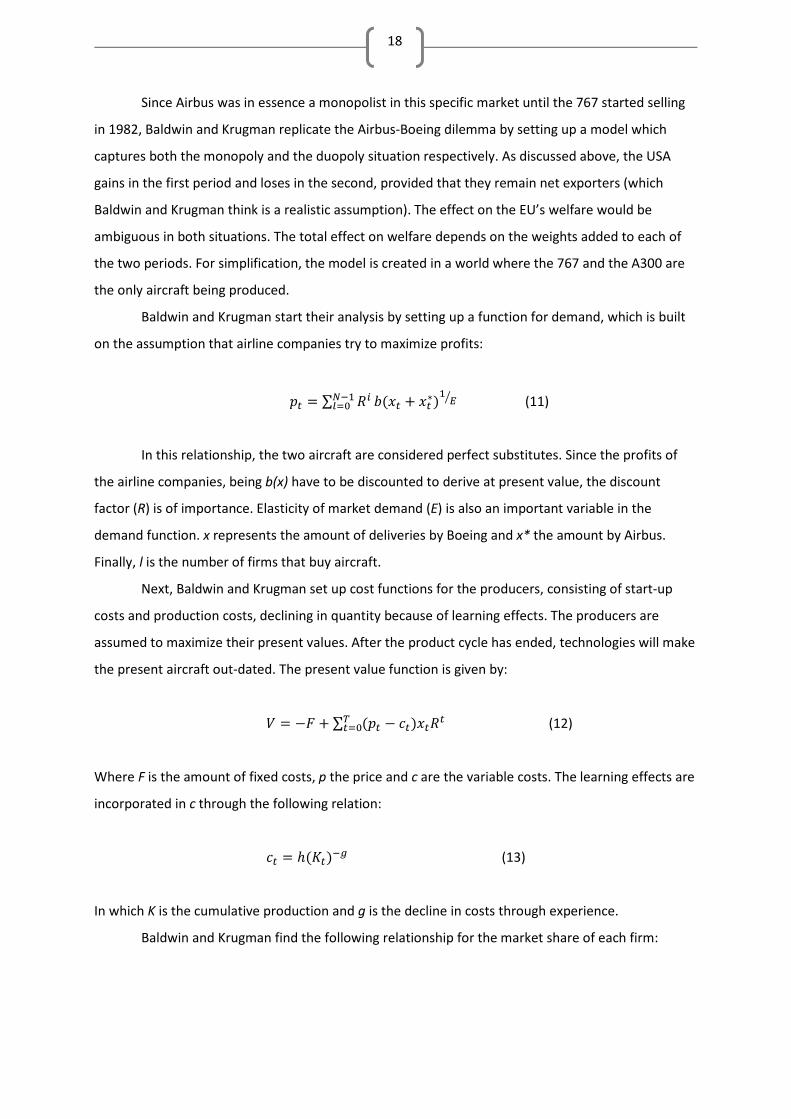
Baldwin and Krugman start their analysis by setting up a function for demand, which is built

on the assumption that airline companies try to maximize profits:

�� = ∑ ����� �(�� + ��

∗)�� (11)

In this relationship, the two aircraft are considered perfect substitutes. Since the profits of

the airline companies, being b(x) have to be discounted to derive at present value, the discount

factor (R) is of importance. Elasticity of market demand (E) is also an important variable in the

demand function. x represents the amount of deliveries by Boeing and x* the amount by Airbus.

Finally, l is the number of firms that buy aircraft.

Next, Baldwin and Krugman set up cost functions for the producers, consisting of start-up

costs and production costs, declining in quantity because of learning effects. The producers are

assumed to maximize their present values. After the product cycle has ended, technologies will make

the present aircraft out-dated. The present value function is given by:

� = −� + ∑ (����� − ��)��

� (12)

Where F is the amount of fixed costs, p the price and c are the variable costs. The learning effects are

incorporated in c through the following relation:

�� = ℎ(��)�� (13)

In which K is the cumulative production and g is the decline in costs through experience.

Baldwin and Krugman find the following relationship for the market share of each firm:

19

s=

1-m�1-1E�

�1E��1+m�

(14)

In which E again is the elasticity of demand and m is the ratio of foreign firm marginal costs to home

firm marginal costs. The amount of deliveries Boeing and Airbus make can be derived from the

demand and the market share functions.

In their next chapter, Baldwin and Krugman calibrate the model to the situation of Airbus and

Boeing. They insert the subsidy in this model by arguing that the discount rate for Airbus is pushed

down until entry is just profitable, using the number zero. For Boeing a discount rate of 5% is

estimated. The learning curve elasticity is taken as 0.2 and the initial set-up costs as 1.5 billion

dollars, which were derived from industry estimates. Baldwin and Krugman explain that the price

elasticity for this particular market is hard to obtain, because exact prices are not known. They do

find that demand elasticity for the entire aircraft market equals 0.57, but the cross-price effect

(changes in demand due to price changes in other industries/segments) must also be added to this

number. They estimate that the cross-price effect should be between one and two, equalling the

total price elasticity at a range of 1.57-2.57. They explain this range by calculating that when E < 1.57,

the internal rate of return for Airbus is larger than 3.5%, while research showed that the internal rate

of return was most likely negative or barely positive. When E > 2.57, Boeing’s 767 would be an

unprofitable project, which the literature also considers to be highly unlikely. Baldwin and Krugman

end up using E=2 as their price elasticity. They also calculate that Airbus’ direct costs are 17.2%

higher than Boeing’s because of their lack in learning relative to Boeing.

The A300 was introduced in 1979 for a price of $61 million. This price drops throughout its

entire life, but remarkably it drops by less when the 767 first sells in 1982 (see figure 8 below).

Baldwin and Krugman explain that because of intertemporal substitution (i.e. postponing purchases

when lower prices are expected), price drops have not been enormous.

Airbus’ market share decreases from 1982 onwards, because of its lower learning effects

relative to Boeing. The authors conclude that Airbus suffered a loss of $836 million. To calculate the

size of the subsidy, opportunity cost for the public funds must be accounted for. Baldwin and

Krugman calculate that when this number is 3%, cost of the subsidy would be $1294 million, with 5%

$1471 million and with 10% $1672 million. Finally, Baldwin and Krugman find values for the

consumer surplus of the EU, the US and rest of the world.

20

Fig. 8: Simulation results with E=2.0

Baldwin and Krugman (1988, pp. 66-67)

Baldwin and Krugman compare the numbers above, which they refer to as the base case,

with scenarios in which Airbus did not enter the market. In the first scenario, static demand

formulation is being used, where the demand curve is the same as in the base case, despite the fact

that there were zero sales between 1979 and 1981. The second scenario allows for intertemporal

substitution, which Baldwin and Krugman call a more realistic version. This means demand between

1979 and 1981 is shifted towards 1982.

21

In the first scenario, Baldwin and Krugman find that Boeing’s price will be around 40% higher

when it is the only producer. When using a 5% discount rate, EU’s surplus is about $2.5 billion higher

in the presence of Airbus. Since the cost of the subsidy is about $1.5 billion in this case, Europe would

gain around $1 billion. When future cash flows are discounted against a lower rate, welfare gain is

higher. Baldwin and Krugman show that in this scenario, Europe will just lose when the discount rate

is as much as 10%, so will gain when it is lower than 10%. Boeing’s profits will drop by $3.2 billion

using the 5% discount rate and consumer surplus should rise by $4 billion, resulting in a gain of $800

million. The US will also lose when discount rates are 10%. Compared to this scenario the rest of the

world would gain between $1.8 and $4 billion in consumer surplus with Airbus.

Compared to the second scenario, including intertemporal substitution, the EU will gain $0.6

billion at 3%, will just lose when the discount rate equals 5% and lose $900 million at 10%. The US

will lose $3.0 billion at 5%, $2.3 billion at 3% and $4.0 billion at a 10% discount rate. The rest of the

world will gain between $0.9 and $2.4 billion (all results are in the figure above).

Since the latter scenario is considered the more realistic one, the overall conclusion by

Baldwin and Krugman is that Europe itself loses at any discount rate above 3%. Moreover the US will

lose at any discount rate and this loss dominates the gain in consumer surplus around the world. This

indicates that the BS model only holds when discount rates are smaller than 3%.

Section IV-C: Entry into the market for large transport aircraft

In his research on this item, Klepper (1990) creates a capacity game in which he tries to find out what

time it takes for a late entrant like Airbus to omit its disadvantage. In contrast to Baldwin and

Krugman as discussed above, Klepper does focus on the entire aircraft market instead of just the

A300 versus the 767. However, McDonnell-Douglas is also left out, because according to Klepper, it

has not developed a new aircraft and would perhaps not stay in the market for commercial jets. In

the model, firms are assumed to produce identical aircraft in each of the market segments and have

the same cost function, but the incumbent firm can be further in its learning curve and thus have

lower marginal costs. The optimal capacity choice is obtained by the interception of the reaction

curves in Cournot-Nash equilibrium.

Klepper divides the aircraft industry into three segments, being S (short-range, narrow body),

M (short/medium-range, wide body) and L (long range, wide body). He predicts the demand in each

of these segments for the period 1987 till 2006 based on estimations by the aircraft manufacturers

themselves. Klepper agrees to Baldwin and Krugman that exact prices of jets are hard to obtain, so

he uses average prices which are modelled as being constant. Next, for calibration purposes, Klepper

22

finds the size of the start-up costs and the learning elasticity. For the learning elasticity he finds 0.2,

which equals the amount Baldwin and Krugman used in their paper. Klepper argues this value is

widely accepted. Finally, price elasticities are endogenous in this model and a return of 5.5% is

arbitrarily chosen,

Klepper uses the actual number of jets produced by either firm in all three market segments

to make a prediction about the period 1986-2006. The amount of aircraft already produced (before

1986) decides the amount of experience the firm already has in this segment and adds to the amount

of experience obtained while producing in the predicted period. This already obtained experience

lowers marginal costs. Klepper finds that in market segment S, Boeing has a marginal cost advantage

of 23% which results in a 69% market share. For market segment M, Airbus has a 6% advantage with

respect to costs, because of the fact that the A300 was produced before the 767 (remember from

Baldwin and Krugman that Airbus had a monopoly from 1979-1982 in this segment). Because of this

advantage, Airbus obtains a 53% market share. In segment L, Boeing starts off with experience

because of its 747, resulting in 15% lower marginal costs, giving it a market share of 55%. These

results are shown in figures 9 and 10 below.

Fig. 9: Production up to 1987

Klepper (1990, p. 787)

Fig. 10: 1987-2006 base case calibration

Klepper (1990, p. 787)

Klepper shows that in the period 1986-2006 both Airbus and Boeing would be profitable, but

Airbus would not reach break-even at the end of 2006 due to its severe losses at the start-up. The

numbers obtained here will be described as the base case, which is shown below in figure 11.

23

Fig. 11: Revenues, costs and profits (billion $)

Klepper (1990, p. 788)

Note that Baldwin and Krugman considered Airbus to be a losing producer in their

assumptions (cost curve above demand) and that these results seem to justify their assumption,

because the overall net profit margin has a negative value. When Baldwin and Krugman considered

their demand elasticity, they have assumed Boeing’s 767 to be a profitable project. Since the 767 was

first sold in 1982 and therefore finds itself in both the ‘prior to 1987’ and the ‘1987-2006’ period,

which have negative and positive return respectively, it is hard to say whether this assumption is

justified by Klepper’s research. Also, Klepper uses all aircraft by Boeing and not just the 767.

Klepper compares the base case to two other scenarios, both where Airbus stays out of the

market. In the first scenario Boeing obtains a monopoly position and in the second scenario, Boeing

will form a duopoly, not with a new entrant like Airbus, but together with an already producing firm.

In the monopoly case, Boeing’s return will increase from 12.5 to 27%, around 20% less aircraft will be

produced at a 3-16% higher price. In the duopoly case, the amount of experience of both firms is

completely equal, giving them the same amount of marginal costs and market share (Note that this

will probably not be the case, since all literature suggests that Boeing dominated the market for

aircraft before Airbus entered). In this scenario, Klepper finds that the profits the two firms make

together is substantially less than in the base case, but output and prices are barely changed. This is

due to the strong scale effects. The comparison between the base case and the two scenarios are

displayed in figures 12 and 13 below.

24

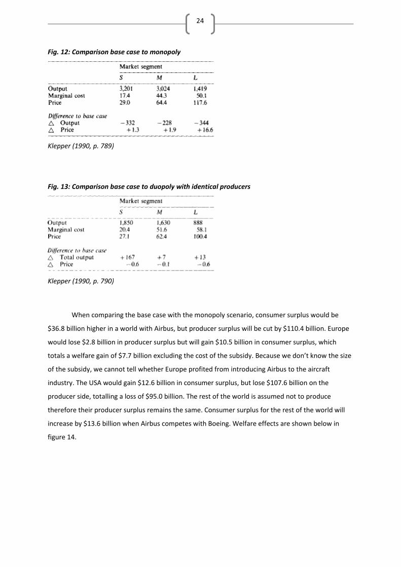
Fig. 12: Comparison base case to monopoly

Klepper (1990, p. 789)

Fig. 13: Comparison base case to duopoly with identical producers

Klepper (1990, p. 790)

When comparing the base case with the monopoly scenario, consumer surplus would be

$36.8 billion higher in a world with Airbus, but producer surplus will be cut by $110.4 billion. Europe

would lose $2.8 billion in producer surplus but will gain $10.5 billion in consumer surplus, which

totals a welfare gain of $7.7 billion excluding the cost of the subsidy. Because we don’t know the size

of the subsidy, we cannot tell whether Europe profited from introducing Airbus to the aircraft

industry. The USA would gain $12.6 billion in consumer surplus, but lose $107.6 billion on the

producer side, totalling a loss of $95.0 billion. The rest of the world is assumed not to produce

therefore their producer surplus remains the same. Consumer surplus for the rest of the world will

increase by $13.6 billion when Airbus competes with Boeing. Welfare effects are shown below in

figure 14.

25

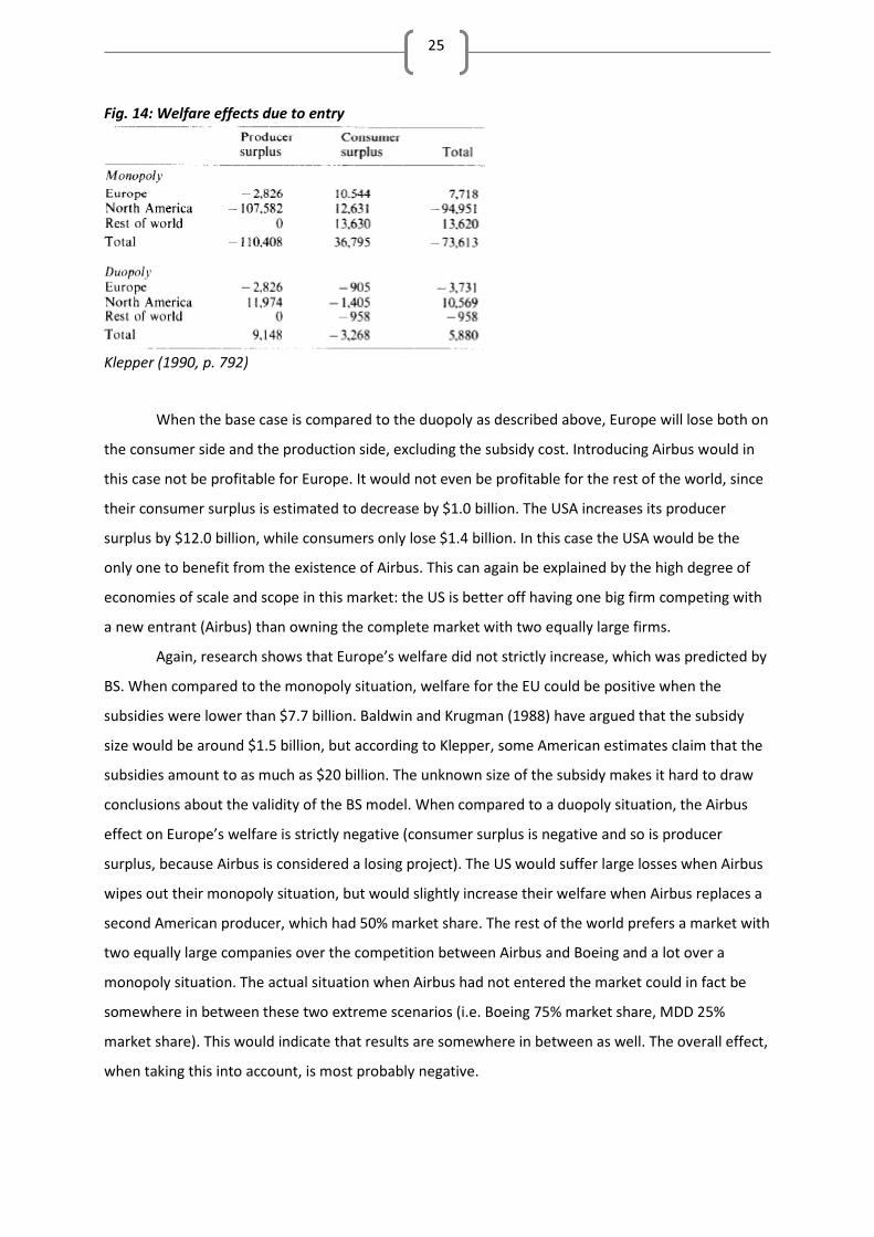
Fig. 14: Welfare effects due to entry

Klepper (1990, p. 792)

When the base case is compared to the duopoly as described above, Europe will lose both on

the consumer side and the production side, excluding the subsidy cost. Introducing Airbus would in

this case not be profitable for Europe. It would not even be profitable for the rest of the world, since

their consumer surplus is estimated to decrease by $1.0 billion. The USA increases its producer

surplus by $12.0 billion, while consumers only lose $1.4 billion. In this case the USA would be the

only one to benefit from the existence of Airbus. This can again be explained by the high degree of

economies of scale and scope in this market: the US is better off having one big firm competing with

a new entrant (Airbus) than owning the complete market with two equally large firms.

Again, research shows that Europe’s welfare did not strictly increase, which was predicted by

BS. When compared to the monopoly situation, welfare for the EU could be positive when the

subsidies were lower than $7.7 billion. Baldwin and Krugman (1988) have argued that the subsidy

size would be around $1.5 billion, but according to Klepper, some American estimates claim that the

subsidies amount to as much as $20 billion. The unknown size of the subsidy makes it hard to draw

conclusions about the validity of the BS model. When compared to a duopoly situation, the Airbus

effect on Europe’s welfare is strictly negative (consumer surplus is negative and so is producer

surplus, because Airbus is considered a losing project). The US would suffer large losses when Airbus

wipes out their monopoly situation, but would slightly increase their welfare when Airbus replaces a

second American producer, which had 50% market share. The rest of the world prefers a market with

two equally large companies over the competition between Airbus and Boeing and a lot over a

monopoly situation. The actual situation when Airbus had not entered the market could in fact be

somewhere in between these two extreme scenarios (i.e. Boeing 75% market share, MDD 25%

market share). This would indicate that results are somewhere in between as well. The overall effect,

when taking this into account, is most probably negative.

26

Section IV-D: Adding a third producer

Both Baldwin and Krugman (1988) and Klepper (1990) have modelled the situation as duopolies in

their studies, while in fact MDD did not merge with Boeing until 1997. According to Klepper, MDD’s

market share was around 10-15% at the time of his research. Neven et al.’s (1995) analysis differs

from the previous two, mainly because of the fact that in their analysis Airbus will be the third

producer, joining both Boeing and MDD.

Neven et al. divide the aircraft market in four segments and the time period, running from

the early 1960s until the late 1990s, in six stages. In each stage, all three firms will decide whether or

not to enter each market segment. When a firm decides to enter a specific segment, it bases its

output level on the output set by its rivals (Cournot competition). Production is assumed to take five

years and each jet will have a useful life of 25 years. Economies of scale are reflected by a decrease in

marginal costs when a firm has already produced in earlier stages, even when production took place

in different segments (economies of scope). Marginal costs will decrease by 20% when output is

doubled, indicating a learning elasticity of 0.2 as we have also seen in the previous papers.

The model is solved using backward induction: parameter values and historical data are used

to calculate maximum profits for each scenario at the final stage (i.e. Boeing enters segment one,

Airbus and MDD enter segment two, neither enters segment three or four). In this final stage, the

Nash equilibrium is assumed to be the outcome that will occur in the future (Note that Neven et al.

do not yet know the outcome of the final period, because their paper was written in 1995, whereas

the final period runs until the late 1990s). Next, they calculate output for each firm, matching the

Nash equilibrium and use these numbers to find the solution for the previous stage. They repeat this

sequence until they find a complete solution for all time periods.

Two important things must be noted at this point. First, production does not necessarily

occur at the Nash equilibrium and second, there can be multiple Nash equilibria. Considering the first

point, Neven et al. do assume that past production decisions were optimal, thus at the Nash

equilibrium, but are aware that this could not hold in reality. Considering the second point, the

authors do indeed find different Nash equilibria for several time periods, but at the end of their

calculations, only a single Nash equilibrium in each stage fits the overall solution.

To compare the base case with the case when Airbus does not enter, the authors obviously

leave Airbus out of the analysis in the first place, but also incorporate that Boeing and MDD are able

to produce at lower marginal costs due to increased output. Figure 15 below shows their results.

27

Figure 15: Base case results

Neven et al. (1995, p. 335)

Neven et al. agree that elasticity of demand is the hardest parameter to estimate and for this

reason they have decided to run the analysis twice, based on two different values. The absolute

values are not mentioned, but ‘High’ elasticity of demand is 20% higher than ‘Low’.

An important conclusion is that although its overall profit declines in a market with Airbus,

MDD is better off in certain segments. This can be explained by the fact that Airbus’ entry reduces

Boeing’s enormous economies of scale and scope, so that in a segment where Boeing and MDD

compete head to head, MDD has actually an increased market share. They say that when Airbus had

not entered the market, MDD would probably not have developed the MD11 to compete with

Boeing’s 777.

As can be seen in figure 15, consumer surplus and prices are showed unadjusted and

adjusted for quality. It is assumed that when firms produce new aircraft rather than continue the

production of older models, quality is improved. It can first be noticed that when Airbus enters the

market, Boeing’s profits will decrease by between $103 and $152 billion, MDD’s profits will lower by

$9 to $24 billion, prices will drop between 0 and 6% and consumer surplus will increase by $5 to $39

billion. Second, it can be noticed that with the adjustment for quality, Airbus’ effect on the increase

in consumer surplus and the decrease in prices is less significant. This indicates that when Airbus is in

the market, producers tend to be less innovative. As mentioned earlier in this paper, R&D costs are

very high in this industry, making firms better off selling older models when profits are lower rather

than developing new ones. Again, the decrease in profits is mostly due to the loss of economies of

scale through the decrease in learning. Finally, the figure shows that Airbus’ effects are more

significant during the last four periods, which run from the moment Airbus officially entered the

market until the late 1990s, but this does indicate that during the stages before the entry of Airbus,

28

Boeing and MDD already responded lightly to the announced entry of Airbus by lowering their

supply.

Neven et al. conclude that the price drop on average equals 3.5%, which they think is a minor

effect. They believe that enough competition for Boeing was already provided by MDD. They also

conclude that Airbus had a positive effect on European welfare, based on its rate of return (although

the size of the subsidy is left out, because subsidies are not considered in this model). Neven et al.

finally conclude that Airbus has had a large negative impact on world welfare, applying equal weights

to consumer surplus and profits. However, this large negative effect is mostly due to the extreme

losses Boeing faces and is thus a negative effect for the USA only. In the figure above it can be seen

that consumer surplus always increases in the presence of Airbus and it can therefore be stated that

the rest of the world (excluding the USA) will be better off with Airbus.

Section V: Conclusions

The BS model states that subsidies increase domestic welfare, decrease foreign welfare and increase

world’s welfare due to lower prices. In this paper, empirical evidence for the validity of the model is

reviewed.

Baldwin and Flam (1989) find that in the market for commuter aircraft the BS model holds,

since Brazil raises its welfare at the expense of its rivals’ welfare and increases rest of the world’s

welfare by subsidizing its domestic firm. Daltung et al. (1987) and Laussel et al. (1988) also find

evidence in favour of the BS model in the ski production and car market respectively. However,

Baldwin and Krugman (1986) conclude that Japan’s import restriction, which is a comparable

strategic trade policy, carried more costs than revenues. In addition, Smith (1994), who also tests the

European car market, finds that strategic trade policy usually decreases producer surplus by more

than consumer surplus increases, indicating that BS does not hold. Based on this evidence it is hard

to draw a general conclusion.

The next aim of this paper is to find if the BS model holds in the Airbus-Boeing dilemma.

Baldwin and Krugman (1988) have created a model in which Airbus will first be a monopolist in the

market for medium-range, wide-bodied aircraft, but shares this market with Boeing during later

years. Their main conclusions are that Europe will most likely lose in terms of welfare pursuing this

strategic trade policy. Only when the discount rate is at or lower than 3% Europe’s increase in

consumer surplus would outweigh its cost of the subsidy. This result indicates that the BS model only

holds when the discount rate is lower than 3%. According to Baldwin and Krugman the USA suffers

big losses in welfare, because the decrease in producer surplus dominates the increase in consumer

29

surplus. The rest of the world, excluding the EU and the US, wins because of increasing levels of

consumer surplus through price decreases. When the gains and losses of the EU, the US and the rest

of the world are combined, the introduction of Airbus seems to be an overall welfare decreasing

strategy. Klepper’s (1990) research seems to contribute to the conclusion drawn by Baldwin and

Krugman that Airbus’ effect on Europe’s welfare is ambiguous. They show that when a duopoly

between Airbus and Boeing is compared to a monopoly by the latter, welfare effects for the EU are

unclear, depending on the actual size of the subsidy, welfare effects for the US are highly negative

and welfare effects for the rest of the world are positive, but relatively small. When a duopoly

between Airbus and Boeing is compared to a duopoly in which two American firms have equal

market shares, welfare effects due to Airbus are strictly negative for the EU and for the rest of the

world, but are positive for the US. The US has a higher producer surplus when Boeing competes with

relatively small Airbus than with an equally sized American firm. Overall, the entry of Airbus seems to

be a welfare decreasing strategy. In addition, Klepper shows that based on his calibration that runs

until 2006, Airbus does not break even. This indicates that at least until 2006, Airbus is not a

profitable project. Neven et al. (1995) try to model the situation more realistically by also considering

MDD in the market. When Airbus enters a market in which Boeing and MDD compete, they show

that MDD will be better off in certain segments in which it competes head-to-head with Boeing.

Overall, Boeing and MDD are worse off with Airbus’ entry. Neven et al. show that Airbus is in fact

profitable and therefore increases Europe’s welfare. However, since subsidies were not considered in

this research, the total effect on Europe’s welfare is still dubious. Neven et al. moreover conclude

that the US has suffered big losses due to this strategic trade policy and prices of aircraft were only

reduced by 3.5%. They conclude that the overall effect due to Airbus is highly negative.

Even though the aircraft market connects the most to the assumptions imposed by Brander

and Spencer and the empirical research uses the same equilibrium model, which seemed to be of

critical importance, evidence suggests that the Brander-Spencer model did not hold in the Airbus-

Boeing dilemma.

Section VI: Discussion

All authors are very cautious about making statements, because certain parameters, like elasticities

and the appropriate discount rates are not known and can create a vital difference in the outcome.

Therefore, all evidence in this paper is far from conclusive, but does suggest that the BS argument did

not hold in this event. Interestingly enough, it did seem to hold in the paper by Baldwin and Flam

(1989), despite the fact that the markets for commercial and commuter aircraft seem very similar.

Baldwin and Flam have shown that Brazil loses when no export subsidy is given, just like both

30

Baldwin & Krugman and Klepper respectively assumed and calculated about Airbus’ profits. However,

Baldwin and Flam do find that Brazil makes a large profit after the subsidy is received, whereas

research in the Airbus-Boeing case (except for Neven et al.) considers Airbus to be losing even with

governmental aid. This seems to explain the different outcomes. Baldwin & Flam and Neven et al. do

produce similar outcomes (which fortifies the statement above), but Neven et al. do not calculate the

size of the subsidy, while Baldwin and Flam do estimate an optimal value of the subsidy. Estimating

the total size of the European subsidies given to Airbus seems to be hard, based on the wide range of

predictions about this number. Neven et al.’s research might be the most relevant since it is the most

recent paper, but the total value of the subsidy or subsidies is still unknown. Without the total

subsidy value, Europe’s changes in welfare cannot be known with certainty.

31

References

Baldwin, R., & Flam, H. (1989). Strategic trade policies in the market for 30–40 seat commuter

aircraft. Weltwirtschaftliches Archiv, 125(3), 484-500.

Baldwin, R., & Krugman, P. R. (1986). Market access and international competition: a simulation

study of 16K random access memories.

Baldwin, R., & Krugman, P. (1988). Industrial policy and international competition in wide-bodied jet

aircraft. In Trade policy issues and empirical analysis (pp. 45-78). University of Chicago Press.

Brander, J. A., & Spencer, B. J. (1985). Export subsidies and international market share rivalry. Journal

of international Economics, 18(1), 83-100.

Carbaugh, R., & Olienyk, J. (2001). Boeing-Airbus Subsidy Dispute: An Economic and Trade

Perspective. Global Economy Quarterly, 2(4), 261-82.

Daltung, S., Eskeland, G., & Norman, V. D. (1987). Optimum trade policy towards imperfectly

competitive industries: Two Norwegian examples (No. 218). CEPR Discussion Papers.

Dixit, A. K., & Grossman, G. M. (1986). Targeted export promotion with several oligopolistic

industries. Journal of International Economics, 21(3), 233-249.

Eaton, J., & Grossman, G. M. (1986). Optimal trade and industrial policy under oligopoly. The

Quarterly Journal of Economics, 101(2), 383-406

Horstmann, I. J., & Markusen, J. R. (1986). Up the average cost curve: Inefficient entry and the new

protectionism. Journal of International Economics, 20(3), 225-247.

Klepper, G. (1990). Entry into the market for large transport aircraft. European Economic Review,

34(4), 775-798.

Krugman, P. R. (1987). Is free trade passé?. The Journal of Economic Perspectives, 1(2), 131-144.

Krugman, P.R., Obstfeld, M., & Melitz, M.J. (2012). International Economics: Theory & Policy (9th ed.).

Harlow, Essex, England: Pearson Education Limited.

Laussel, D., Montet, C., & Peguin-Feissolle, A. (1988). Optimal trade policy under oligopoly: a

calibrated model of the Europe-Japan rivalry in the EEC car market. European Economic

Review, 32(7), 1547-1565.

Markusen, J. R., & Venables, A. J. (1988). Trade policy with increasing returns and imperfect

competition: Contradictory results from competing assumptions. Journal of International

Economics, 24(3), 299-316.

Smith, A. (1994). Strategic trade policy in the European car market. In Empirical studies of strategic

trade policy (pp. 67-84). University of Chicago Press.

Neven, D., Seabright, P., & Grossman, G. M. (1995). European industrial policy: The Airbus case.

Economic Policy, 10, 313-358.