stream solute transport incorporating hyporheic zone processes

Journal of Hydrology (2006) 329, 26–38

ava i lab le at www.sc iencedi rec t . com

journal homepage: www.elsevier .com/ locate / jhydro l

Stream solute transport incorporating hyporheiczone processes

Cevza Melek Kazezyılmaz-Alhan a,b, Miguel A. Medina Jr. a,*

a Department of Civil and Environmental Engineering, Duke University, P.O. Box 90287, Durham, NC 27708-0287, USAb Department of Civil Engineering, Auburn University, Auburn, AL 36849-5337, USA

Received 27 August 2004; received in revised form 6 January 2006; accepted 2 February 2006

Summary The behavior of solute transport in pool and riffle, or meandering types of streams, isgreatly influenced by surface/subsurface flow and solute transport interactions. It is important tomodel these processes accurately in rivers and streams to improve downstream water quality.Two decades ago, Bencala and Walters (1983) [Bencala, K.E., Walters, R.A., 1983, Simulationof solute transport in a mountain pool-and-riffle stream – a transient storage model. WaterResources Research 19(3), 718–724] introduced the transient storage model to represent themovement of solute from main streams into stagnant zones and back to the main stream. Thismodel includes the effect of both surface storage, in which water is stationary relative to themain channel and the hyporheic zone, to which water moves from the main channel, flowsthrough and returns to the main channel. However, their simplified approach lumped the surfacestorage and hyporheic zones together in a single storage zone. In this study, we take a steptowards a mechanistic model to explain the physics of water exchange between the surfacewater and the porous media by developing an improved mathematical model. For this purpose,we include the advection and dispersion processes into the transient storage zone, and we con-sider the hyporheic zone as a transient porous media from surface water to ground water. We usethis improved model to solve a test problem in order to demonstrate its capabilities. Finally, wesimulate the Uvas Creek experiment and compare our results to the observations described inBencala and Walters (1983) [Bencala, K.E., Walters, R.A., 1983, Simulation of solute transportin a mountain pool-and-riffle stream – a transient storage model. Water Resources Research19(3), 718–724] and to results of the existing transient storage model obtained by using OTIS.

�c 2006 Elsevier B.V. All rights reserved.

KEYWORDSSurface/subsurface waterinteractions;Hyporheic zone;Transient phenomena;Solute transport;Water quality

0d

5

022-1694/$ - see front matter �c 2006 Elsevier B.V. All rights reserveoi:10.1016/j.jhydrol.2006.02.003

* Corresponding author. Tel.: +1 919 660 5195; fax: +1 919 660219.E-mail address: [email protected] (M.A. Medina).

Introduction

There has been a growing interest in understanding themechanisms involved in surface water/subsurface water

d.

mailto:[email protected]

Stream solute transport incorporating hyporheic zone processes 27

interactions since these interactions play a crucial role inthe behavior of contaminant transport both in streams andground water. There are several important factors in deter-mining the concentration distribution and these have beeninvestigated in the past. However, the relevance of thesesurface/subsurface water interactions has been moreacutely understood recently (Hakenkamp et al., 1993; Win-ter et al., 1998; Packman and Bencala, 2000; Bencala, 2000;Medina et al., 2002); consequently, many issues remainunresolved. Surface/subsurface water interactions influ-ence downstream water quality significantly since the con-centration distribution both in a stream and in groundwater changes due to this exchange and biogeochemicalreactions occur between the minerals in the subsurfaceand the minerals in the streams.

Several issues have been raised in the literature with dif-ferent perspectives (e.g., analytical methods, numericalmethods, field methods, or chemical methods) which re-quire further investigation. Among these issues, describingmathematically the hyporheic zone by incorporating rele-vant physical processes is a key goal towards developing abetter understanding of the effect of surface/subsurfacewater interactions on contaminant (solute) transport. Thehyporheic zone is defined as a porous area which connectsstream water and subsurface water that results in exchangeof water between two different media (Bencala, 2000; Run-kel et al., 2003). Runkel et al. (2003) emphasize the role ofthe hyporheic zone concept in solute transport in streams.They summarize the ongoing research efforts on modelinghyporheic zone processes and point out that many chal-lenges still remain. The areas of suggested further researchare summarized as: (i) improvement of existing stream tra-cer approaches; (ii) solution for scale issue problems; and(iii) improvement of field and modeling techniques. In thisstudy, we focus on the improvement of the existing streamtracer approach. Particularly, an improved mathematicalmodel for describing the hyporheic zone is introduced.

Much progress has been made in modeling transient stor-age zone processes in the last two decades. Bencala andWalters (1983) and Bencala (1983) initiated a first stepand sparked a large horizon of research interest by develop-ing a transient storage model. Jackman et al. (1984) de-scribed three different conceptual models to representthe transient storage of solute in the streambed: (1) the ex-change model, (2) the diffusion model, and (3) the under-flow model. The exchange model assumes a uniformconcentration in the streambed and the flux of solute is pro-portional to the difference between the streambed and thestream concentration. The diffusion model assumes solutetransport in the vertical direction within the bed, describedby Fick’s law. The underflow model assumes a convectivechannel in one portion of the bed through which streamwater flows by entering at one location and returning tothe stream at another location, and the exchange model isused to describe storage throughout the rest of the bed asthe underflow model considers the existence of only oneconvective channel in the bed. They concluded thatalthough all three models can predict concentrations rea-sonably well, the second and third model seem somewhatsuperior than the first model.

Wagner and Gorelick (1986) developed a nonlinear multi-ple-regression method to estimate the parameters of con-

taminant transport and the transient storage model. Theyobtained better fits for the Uvas Creek experiment con-ducted in California than Bencala and Walters (1983). Later,Runkel and Chapra (1993) worked on efficient numericalmethods to solve the coupled transient storage equations.They decreased the computational time by two differentmethods, decoupling the differential equations and usingthe Thomas algorithm. Harvey et al. (1996) conducted astream tracer experiment at St. Kevin Gulch to evaluatethe reliability of the stream tracer approach in determininga characteristic length and time scale. By injecting a solutetracer to characterize the hyporheic zone processes, theyfound that the stream tracer approach is not sensitive toall time scales and did not provide reliable results at highbase flow. Worman (1998) developed a new model for thesolute transport which includes the effect of hyporheic zoneexchange, sorption and first order reaction. He derived ananalytical solution for this model which describes thestream concentration as a function of distance along thestream, depth into the storage zone and time. Runkel R.L.(1998) developed a well known code (one-dimensionaltransport with inflow and storage model, OTIS), whichsolves the transient storage equations to simulate solutetransport in streams and rivers. He later coupled a kine-matic wave routing model with OTIS to analyze transientstorage in streams with quasi-unsteady flow, and conducteda tracer experiment in Huey Creek to quantify the interac-tions (Runkel et al., 1998). He recently completed a thor-ough study to introduce a new metric to determine theimportance of transient storage (Runkel, 2002). Scottet al. (2003) studied a parameter estimation method whichis automated calibration inverse modeling for estimation ofparameters of the transient transport model. Lin and Medi-na (2003) developed a model which incorporates transientstorage in conjunctive stream-aquifer modeling.

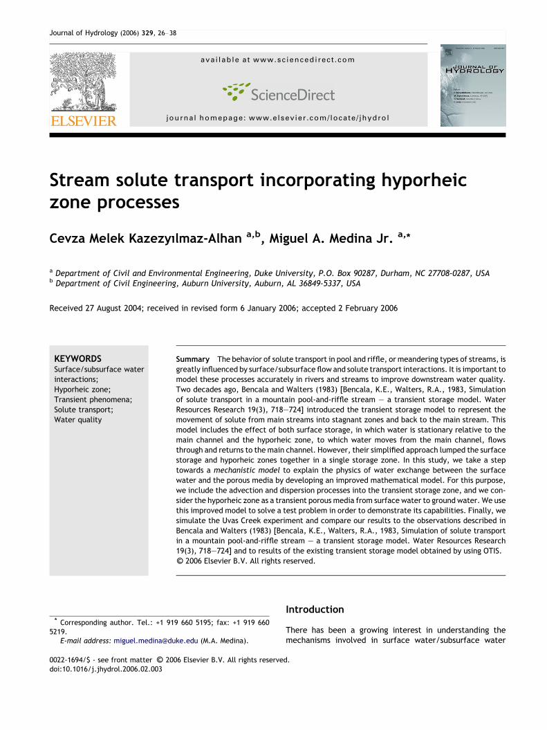
In this study, we attempt to improve the transient stor-age model introduced by Bencala and Walters (1983) andBencala (1983). Their transient storage model couples theeffect of the dead zone (Fig. 1A, in which water is immobilerelative to water in the main channel) and the effect of thehyporheic zone (where stream water moves into groundwater flow paths and returns to the stream, Fig. 1B) throughthe stream advection-dispersion equation. This model initi-ates the concept of transient storage and provides an under-standing of the behavior of solute transport in streams dueto surface/subsurface water interactions. However, as sta-ted by Runkel et al. (2003), there is still room for improve-ment: ‘‘This model is an empirical approach that does notattempt to model exchange in a mechanistic manner. Fur-ther, surface storage (Fig. 1A) and hyporheic exchange(Fig. 1B) are lumped together in a single storage zone’’.Therefore, our study aims to improve the existing transientstorage model by taking a step towards a more mechanisticrepresentation of surface/subsurface water interactionswith an improved mass-transport model.

The objectives of this study are: (1) to present an im-proved mathematical model to represent the hyporheiczone processes and model the effects of surface/subsurfacewater interactions on solute transport with a more physi-cally realistic transient storage model; (2) to develop anumerical solution with an implicit finite difference schemefor the new model; (3) to present the results of the model

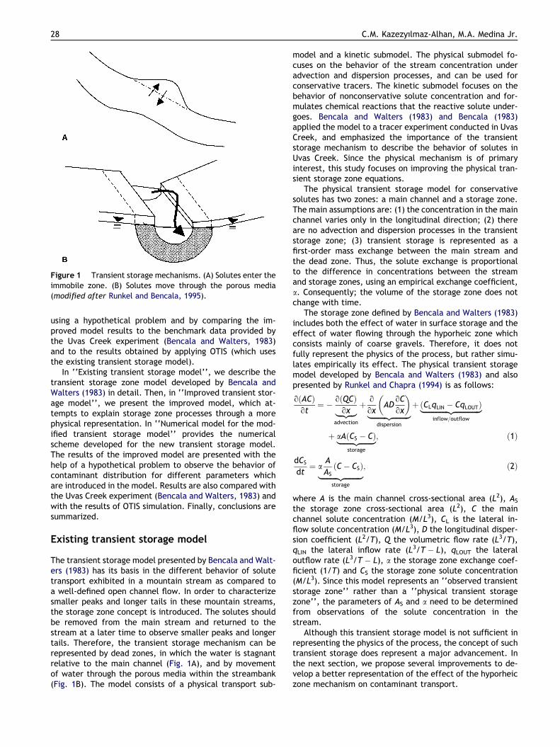
Figure 1 Transient storage mechanisms. (A) Solutes enter theimmobile zone. (B) Solutes move through the porous media(modified after Runkel and Bencala, 1995).

28 C.M. Kazezyılmaz-Alhan, M.A. Medina Jr.

using a hypothetical problem and by comparing the im-proved model results to the benchmark data provided bythe Uvas Creek experiment (Bencala and Walters, 1983)and to the results obtained by applying OTIS (which usesthe existing transient storage model).

In ‘‘Existing transient storage model’’, we describe thetransient storage zone model developed by Bencala andWalters (1983) in detail. Then, in ‘‘Improved transient stor-age model’’, we present the improved model, which at-tempts to explain storage zone processes through a morephysical representation. In ‘‘Numerical model for the mod-ified transient storage model’’ provides the numericalscheme developed for the new transient storage model.The results of the improved model are presented with thehelp of a hypothetical problem to observe the behavior ofcontaminant distribution for different parameters whichare introduced in the model. Results are also compared withthe Uvas Creek experiment (Bencala and Walters, 1983) andwith the results of OTIS simulation. Finally, conclusions aresummarized.

Existing transient storage model

The transient storage model presented by Bencala and Walt-ers (1983) has its basis in the different behavior of solutetransport exhibited in a mountain stream as compared toa well-defined open channel flow. In order to characterizesmaller peaks and longer tails in these mountain streams,the storage zone concept is introduced. The solutes shouldbe removed from the main stream and returned to thestream at a later time to observe smaller peaks and longertails. Therefore, the transient storage mechanism can berepresented by dead zones, in which the water is stagnantrelative to the main channel (Fig. 1A), and by movementof water through the porous media within the streambank(Fig. 1B). The model consists of a physical transport sub-

model and a kinetic submodel. The physical submodel fo-cuses on the behavior of the stream concentration underadvection and dispersion processes, and can be used forconservative tracers. The kinetic submodel focuses on thebehavior of nonconservative solute concentration and for-mulates chemical reactions that the reactive solute under-goes. Bencala and Walters (1983) and Bencala (1983)applied the model to a tracer experiment conducted in UvasCreek, and emphasized the importance of the transientstorage mechanism to describe the behavior of solutes inUvas Creek. Since the physical mechanism is of primaryinterest, this study focuses on improving the physical tran-sient storage zone equations.

The physical transient storage model for conservativesolutes has two zones: a main channel and a storage zone.The main assumptions are: (1) the concentration in the mainchannel varies only in the longitudinal direction; (2) thereare no advection and dispersion processes in the transientstorage zone; (3) transient storage is represented as afirst-order mass exchange between the main stream andthe dead zone. Thus, the solute exchange is proportionalto the difference in concentrations between the streamand storage zones, using an empirical exchange coefficient,a. Consequently; the volume of the storage zone does notchange with time.

The storage zone defined by Bencala and Walters (1983)includes both the effect of water in surface storage and theeffect of water flowing through the hyporheic zone whichconsists mainly of coarse gravels. Therefore, it does notfully represent the physics of the process, but rather simu-lates empirically its effect. The physical transient storagemodel developed by Bencala and Walters (1983) and alsopresented by Runkel and Chapra (1994) is as follows:

oðACÞot¼ � oðQCÞ

ox|fflffl{zfflffl}advection

þ o

oxAD

oC

ox

� �|fflfflfflfflfflfflfflfflffl{zfflfflfflfflfflfflfflfflffl}

dispersion

þ CLqLIN � CqLOUTð Þ|fflfflfflfflfflfflfflfflfflfflfflfflfflffl{zfflfflfflfflfflfflfflfflfflfflfflfflfflffl}inflow=outflow

þ aA CS � Cð Þ|fflfflfflfflfflfflffl{zfflfflfflfflfflfflffl}storage

; ð1Þ

dCS

dt¼ a

A

ASC� CSð Þ|fflfflfflfflfflfflfflfflffl{zfflfflfflfflfflfflfflfflffl}

storage

; ð2Þ

where A is the main channel cross-sectional area (L2), AS

the storage zone cross-sectional area (L2), C the mainchannel solute concentration (M/L3), CL is the lateral in-flow solute concentration (M/L3), D the longitudinal disper-sion coefficient (L2/T), Q the volumetric flow rate (L3/T),qLIN the lateral inflow rate (L3/T � L), qLOUT the lateraloutflow rate (L3/T � L), a the storage zone exchange coef-ficient (1/T) and CS the storage zone solute concentration(M/L3). Since this model represents an ‘‘observed transientstorage zone’’ rather than a ‘‘physical transient storagezone’’, the parameters of AS and a need to be determinedfrom observations of the solute concentration in thestream.

Although this transient storage model is not sufficient inrepresenting the physics of the process, the concept of suchtransient storage does represent a major advancement. Inthe next section, we propose several improvements to de-velop a better representation of the effect of the hyporheiczone mechanism on contaminant transport.


Improved transient storage model

In the improved model, the advection and dispersion pro-cesses are included in the transient storage zone, achievinga direct influence upon the stream concentration of the sur-face water interaction with the subsurface water throughthe hyporheic flow. Our main assumptions are that the med-ium is isotropic and that the solute concentration both inthe stream and in the storage zone varies only in the longi-tudinal direction. Our model improves the existing model inthe following ways:

• We incorporate transient storage into the porous mediamodel; i.e., as subsurface storage. This allows us toaccount physically for the processes of advection and dis-persion and the movement of channel flow (and there-fore the solute in the channel water) through thehyporheic zone (Fig. 1B).

• Instead of representing the stream-aquifer interactionusing an explicit inflow/outflow term, the proposedmodel implicitly takes this interaction into accountthrough use of storage terms.

• The representation of the effect of water exchange onstream concentration is achieved by the additionalexchange terms to the original mass transport equationfor the channel and the mass transport equation for thehyporheic zone.

• In the improved model, the exchange terms representthe mass transport due to the mass flux between thetwo media, whereas in the original model the exchangeterms represent the mass transport due to the concentra-tion gradient between the two media. In reality, themass transport due to both the mass flux and the concen-tration gradient should be taken into account. However,in the improved model, we neglect the mass transportdue to the concentration gradient for simplicity andinvestigate the scenario for which the mass flux is thedominant factor in mass transport between the twomedia.

The mass-transport equations for the hyporheic zone andchannel are derived using a control volume approach(Fig. 2). The accumulation, i.e., the rate of change of mass

Aexch

δx

As

Ah

qLout

qLin

Figure 2 Control volume approach for the concentrationdistribution in the stream and storage. The control volume inthe stream, V1, corresponds to the shaded control volume withthick boundaries, while the control volume in the storage zone,V2, corresponds to the clear control volumewith thin boundaries.

in a control volume is given by the difference between theincoming and outgoing mass. As it can be seen fromFig. 2, two different control volumes are selected, one inthe stream (shaded control volume with thick boundariesV1) and the other in the storage zone (clear control volumewith thin boundaries V2), in order to be able to formulatethe rate of change of mass in both media. As shown, themass going into the first control volume (V1) consists ofthe upstream, lateral inflow, and storage zone mass contri-butions. The mass flux from the storage zone into thestream represents the water exchange between the streamand the porous media. The same term is part of the outgoingmass for the second control volume (V2) in the storage zone.Control volume 1 (V1):

Accumulation:o CV1ð Þ

ot; ð3Þ

Incoming mass: CvxAf gjx�dx=2 � ADoC

ox

� ��x�dx=2

þ CSvs;yAexch

� ��xþ CLqLindxf gjx; ð4Þ

Outgoing mass: CvxAf gjxþdx=2 � ADoC

ox

� ��xþdx=2

þ CvyAexch

� ��xþ CqLoutdxf gjx. ð5Þ

Control volume 2 (V2):

Accumulation:o CSV2ð Þ

ot; ð6Þ

Incoming mass: CSvs;xAS

� ��x�dx=2

� ASDSoCS

ox

� ��x�dx=2

þ CvyAexch

� ��x; ð7Þ

Outgoing mass: CSvs;xAS

� ��xþdx=2

� ASDSoCS

ox

� ��xþdx=2

þ CSvs;yAexch

� ��x; ð8Þ

where Aexch = (dx)h and AS = eAhz. If we assume that thestream velocities in the x and y directions are equal in mag-nitude at points where the stream flows into the hyporheiczone and the storage zone velocities in the x and y direc-tions are equal in magnitude at points where the water inhyporheic zone flows back into the stream, (i.e., vx = vy = vand vs,x = vs,y = vs) and combine all the terms, the followingcoupled differential equations for stream and storage zoneare obtained:

o CAð Þot¼ � o

oxCvAð Þ|fflfflfflfflffl{zfflfflfflfflffl}

advection

þ o

oxAD

oC

ox

� �|fflfflfflfflfflfflfflfflffl{zfflfflfflfflfflfflfflfflffl}

dispersion

þ h CSvs � Cvf g|fflfflfflfflfflfflfflfflfflffl{zfflfflfflfflfflfflfflfflfflffl}storage

þ CLqLin � CqLoutf g; ð9Þo eCSð Þ

ot¼ � o

oxCSvseð Þ|fflfflfflfflfflffl{zfflfflfflfflfflffl}

advection

þ o

oxeDS

oCS

ox

� �|fflfflfflfflfflfflfflfflfflffl{zfflfflfflfflfflfflfflfflfflffl}

dispersion

þ h

AhzCv � CSvsf g|fflfflfflfflfflfflfflfflfflfflfflffl{zfflfflfflfflfflfflfflfflfflfflfflffl}storage

.

ð10Þ

Here, h is the interface thickness (L) and Ahz is the hyp-orheic zone area (L2), which are defined as new parame-ters; C is the concentration in channel (M/L3), CS is theconcentration in storage (M/L3), A is the cross-sectionalarea of the channel (L2), v is the velocity in the channel(L/T), qLin is the lateral inflow rate (L3/T � L), qLout isthe lateral outflow rate (L3/T � L), vs is the velocity inthe storage zone (L/T), D is the dispersion coefficient in


channel (L2/T), DS is the dispersion coefficient in the stor-age zone (L2/T), and e is the porosity of the hyporheiczone. The storage terms represent the exchange betweentwo different regions, i.e, the stream and hyporheic zoneand these terms relate the exchange between surfaceand subsurface phases with the velocities of water in thestream and storage under the assumption that the magni-tude of the x and y components of the velocities are equalfor both stream and channel at the interaction points(vx = vy, vsx = vsy). The maximum values for velocities vyand vsy are selected under this assumption. When we com-pare the storage terms of the existing model to the im-proved transient storage model, we observe that in theexisting model the effect of the exchange on the concen-tration is only represented by the difference in concentra-tions between the stream and storage zones using theempirical exchange coefficient, a. On the other hand, inthe improved model, the exchange between the surfaceand subsurface regions is related to the water velocitiesin those regions through another new parameter whichwe refer to as the interface thickness.

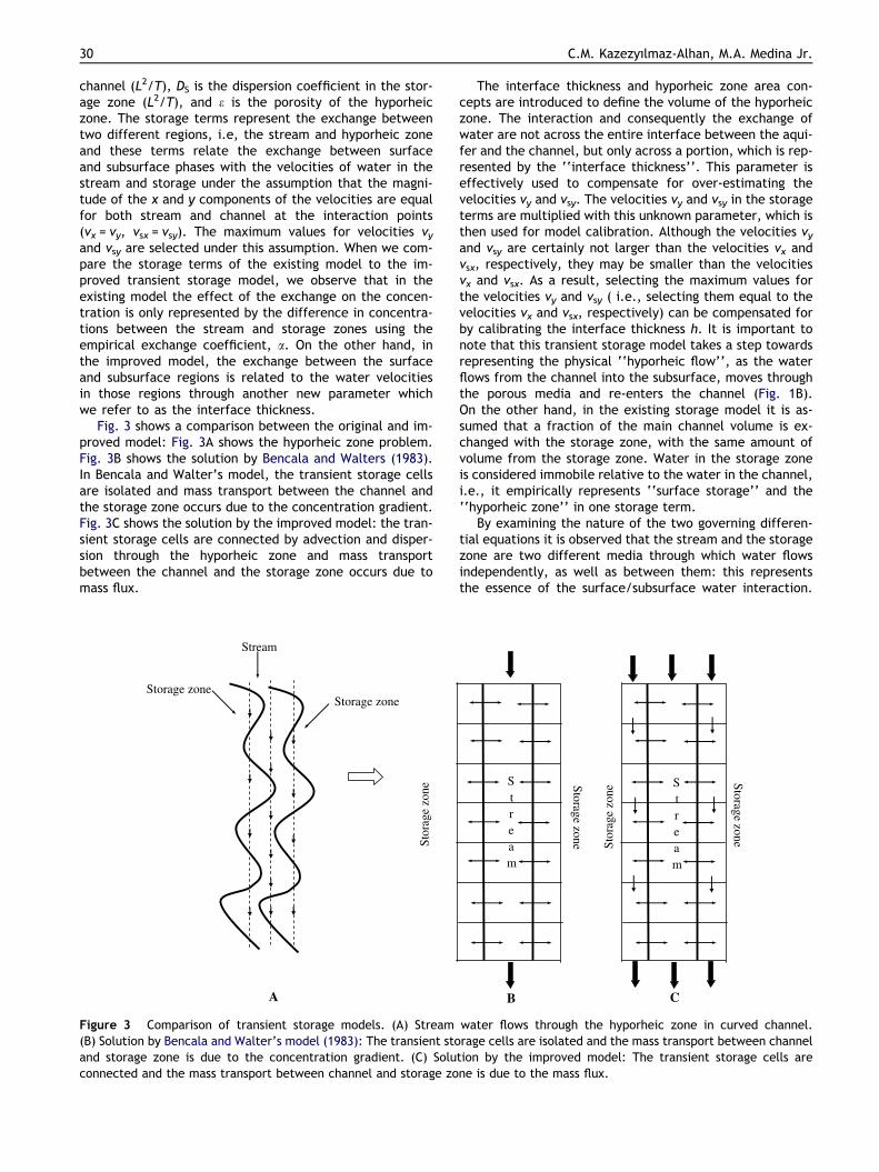
Fig. 3 shows a comparison between the original and im-proved model: Fig. 3A shows the hyporheic zone problem.Fig. 3B shows the solution by Bencala and Walters (1983).In Bencala and Walter’s model, the transient storage cellsare isolated and mass transport between the channel andthe storage zone occurs due to the concentration gradient.Fig. 3C shows the solution by the improved model: the tran-sient storage cells are connected by advection and disper-sion through the hyporheic zone and mass transportbetween the channel and the storage zone occurs due tomass flux.

Stream

Storage zoneStorage zone

Stor

age

zone

A

Figure 3 Comparison of transient storage models. (A) Stream(B) Solution by Bencala and Walter’s model (1983): The transient stoand storage zone is due to the concentration gradient. (C) Soluconnected and the mass transport between channel and storage zo

The interface thickness and hyporheic zone area con-cepts are introduced to define the volume of the hyporheiczone. The interaction and consequently the exchange ofwater are not across the entire interface between the aqui-fer and the channel, but only across a portion, which is rep-resented by the ‘‘interface thickness’’. This parameter iseffectively used to compensate for over-estimating thevelocities vy and vsy. The velocities vy and vsy in the storageterms are multiplied with this unknown parameter, which isthen used for model calibration. Although the velocities vyand vsy are certainly not larger than the velocities vx andvsx, respectively, they may be smaller than the velocitiesvx and vsx. As a result, selecting the maximum values forthe velocities vy and vsy ( i.e., selecting them equal to thevelocities vx and vsx, respectively) can be compensated forby calibrating the interface thickness h. It is important tonote that this transient storage model takes a step towardsrepresenting the physical ‘‘hyporheic flow’’, as the waterflows from the channel into the subsurface, moves throughthe porous media and re-enters the channel (Fig. 1B).On the other hand, in the existing storage model it is as-sumed that a fraction of the main channel volume is ex-changed with the storage zone, with the same amount ofvolume from the storage zone. Water in the storage zoneis considered immobile relative to the water in the channel,i.e., it empirically represents ‘‘surface storage’’ and the‘‘hyporheic zone’’ in one storage term.

By examining the nature of the two governing differen-tial equations it is observed that the stream and the storagezone are two different media through which water flowsindependently, as well as between them: this representsthe essence of the surface/subsurface water interaction.

Storage zone

Stor

age

zone

Stream

Storage zone

CB

Stream

water flows through the hyporheic zone in curved channel.rage cells are isolated and the mass transport between channeltion by the improved model: The transient storage cells arene is due to the mass flux.


If a stream is carefully observed visually, one would identifythe place referred as the hyporheic zone as a porous mediawith a relatively high porosity, since it consists of coarsegravels, goes for a very small distance and acts as a tran-sient zone from the open channel to the aquifer. Therefore,the values of water parameters flowing through the hypor-heic zone are expected to be quantitatively in-betweenthe values of water parameters flowing in the main channeland in the aquifer.

Numerical model for the modified transientstorage model

We solve the modified transient storage model using an im-plicit finite difference method, which is first order backwardin time and second order central in space. The partial dif-ferential equation for the main channel is discretized asfollows:

CAð Þjþ1i � CAð ÞjiDt

¼�CvAð Þjþ1iþ1 � CvAð Þjþ1i�1

2Dx

( )

þADð Þjþ1iþ1=2 Cjþ1

iþ1 �Cjþ1i

�� ADð Þjþ1i�1=2 Cjþ1

i �Cjþ1i�1

�Dxð Þ2

8<:

9=;

þhjþ1i CSvsð Þjþ1i � Cvð Þjþ1i

n oþ CLqLinð Þjþ1i � CqLoutð Þjþ1i

n o;

ð11Þ

ADð Þiþ1=2 ¼ADð Þiþ ADð Þiþ1

2. ð12Þ

After reorganizing, the following finite difference equa-tions for the main channel are obtained:

EiCjþ1i�1 þ FiC

jþ1i þ GiC

jþ1iþ1 þ Pb

i CSjjþ1i

¼ CAð Þji þ CLqLinð Þjþ1i Dt; ð13Þ

where

Ei ¼1

2

DtDx

� vAð Þjþ1i�1

n o� 1

2

Dt

Dxð Þ2ADð Þjþ1i þ ADð Þjþ1i�1

n o; ð14Þ

Fi ¼ Ajþ1i þ 2

Dt

Dxð Þ2ADð Þjþ1i þ Dthjþ1

i vjþ1i þ qLoutð Þjþ1i Dt; ð15Þ

Gi ¼1

2

DtDx

vAð Þjþ1iþ1

n o� 1

2

Dt

Dxð Þ2ADð Þjþ1iþ1 þ ADð Þjþ1i

n o; ð16Þ

Pbi ¼ �h

jþ1i vsjjþ1i Dt. ð17Þ

The finite difference equation for transient storage zoneis derived following a similar methodology to that for themain channel. Since the equations are coupled, the concen-trations in the stream and storage zone are solved simulta-neously. A fixed concentration at the upper boundary and afixed dispersive flux at the lower boundary are used asboundary conditions for both the stream and the hyporheiczone.

In order to verify the accuracy of the numerical solution,we first compare the simulation results for zero interfacethickness (no exchange between two media) with the ana-lytical solutions which exist in the literature for the generaladvection-dispersion equation with constant velocity anddispersion. If the interface thickness, h, is zero, then thestorage terms drop in both differential equations and both

equations reduce to classical advection-dispersion equa-tions for open channel and porous media transport. The ana-lytical solution for the general advection-dispersionequation with a continuous source boundary condition is gi-ven as follows (Bear, 1972):

C x; tð Þ ¼ C0 þ1

2CIN � C0ð Þ erfc

x � vtffiffiffiffiffiffiffiffi4Dtp

� ��

þ expxv

D

�erfc

x þ vtffiffiffiffiffiffiffiffi4Dtp

� ��. ð18Þ

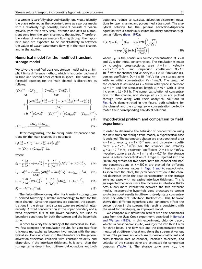
where CIN is the continuous source concentration at x = 0and C0 is the initial concentration. The simulation is madeby choosing cross-sectional area A = 1 m2, velocityv = 1 · 10�3 m/s, and dispersion coefficient D = 1 ·10�2 m2/s for channel and velocity vs = 1 · 10�4 m/s and dis-persion coefficient DS = 1 · 10�3 m2/s for the storage zonewith an initial concentration C0 = 1 mg/l. The length ofthe channel is assumed as L = 100 m with space incrementDx = 1 m and the simulation length tL = 40 h with a timeincrement Dt = 0.1 h. The numerical solution of concentra-tion for the channel and storage at x = 30 m are plottedthrough time along with their analytical solutions inFig. 4. As demonstrated in the figure, both solutions forthe channel and the storage zone concentration perfectlymatch their corresponding analytical solutions.

Hypothetical problem and comparison to fieldexperiment

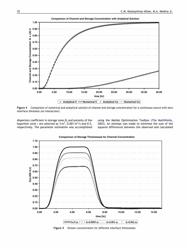
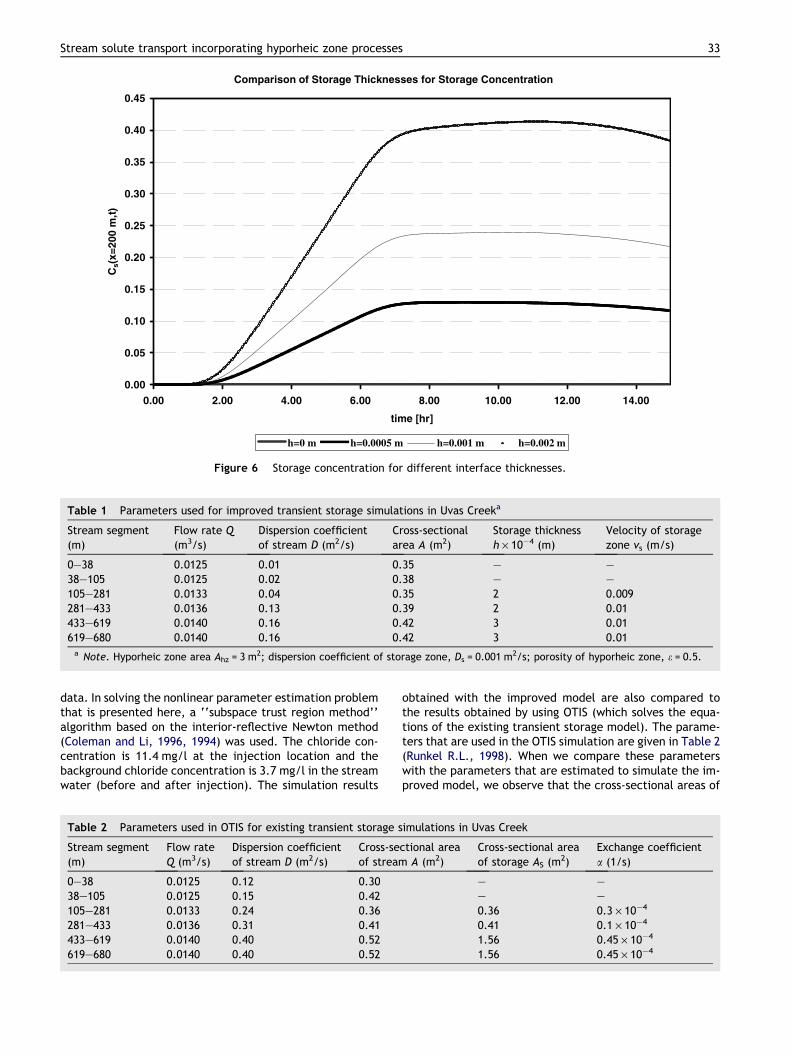
In order to determine the behavior of concentration usingthe new transient storage zone model, a hypothetical caseis designed. The parameters chosen are cross-sectional areaA = 1 m2, velocity v = 3 · 10�2 m/s, and dispersion coeffi-cient D = 2 · 10�1 m2/s for the channel and velocityvs = 3 · 10�3 m/s, dispersion coefficient Ds = 2 · 10�2 m2/s,hyporheic zone area Ahz = 3 m2 and e = 0.7 for the storagezone. A solute concentration of 1 mg/l is injected into the600 m long stream for five hours. Both the channel and stor-age concentrations at x = 200 m are plotted for differentinterface thickness values in Figs. 5 and 6, respectively.As seen from the plots, the peak concentration in the chan-nel decreases while the peak concentration in the storagezone increases with increasing interface thickness. This isan expected behavior since the increase in interface thick-ness allows more interaction between the two differentmedia. Incorporating hyporheic zone processes to streamsolute transport results in different steady-state concentra-tions for different interface thicknesses. This behaviorshows that different hyporheic zone conditions affect theconcentration in the stream: this result is consistent withthe need for developing an improved model.

We compare our simulation results with the benchmarkdata from the Uvas Creek experiment described in Bencalaand Walters (1983). In this experiment, chloride tracer,which is a conservative solute, was injected into Uvas Creekfor three hours. The flow rate and the concentration weremeasured at different locations along the stream at varioustimes. The parameters which are dispersion coefficient andcross-sectional area of channel, interface thickness, andvelocity of the storage zone are estimated for comparisonpurposes (Table 1). The storage zone area Ahz, the

Comparison of Channel and Storage Concentration with Analytical Solution

0.00

0.10

0.20

0.30

0.40

0.50

0.60

0.70

0.80

0.90

1.00

0.00 5.00 10.00 15.00 20.00 25.00 30.00 35.00 40.00

time [hr]

Ch

ann

el a

nd

Sto

rag

eC

on

cen

trat

ion

@ x

=30

m

Analytical C Numerical C Analytical Cs Numerical Cs

Figure 4 Comparison of numerical and analytical solution of channel and storage concentration for a continuous source with zerointerface thickness (no interaction).


dispersion coefficient in storage zone Ds and porosity of thehyporheic zone e are selected as 3 m2, 0.001 m2/s and 0.5,respectively. The parameter estimation was accomplished

Comparison of Storage Thicknes

0.00

0.10

0.20

0.30

0.40

0.50

0.60

0.70

0.80

0.90

1.00

1.10

0.00 2.00 4.00 6.00

ti

C(x

=200

m,t

)

h=0 m h=0.0005 m

Figure 5 Stream concentration for

using the Matlab Optimization Toolbox (The MathWorks,2003). An attempt was made to minimize the sum of thesquared differences between the observed and calculated

ses for Channel Concentration

8.00 10.00 12.00 14.00

me [hr]

h=0.001 m h=0.002 m

different interface thicknesses.

Comparison of Storage Thicknesses for Storage Concentration

0.00

0.05

0.10

0.15

0.20

0.25

0.30

0.35

0.40

0.45

0.00 2.00 4.00 6.00 8.00 10.00 12.00 14.00

time [hr]

Cs(

x=20

0 m

,t)

h=0 m h=0.0005 m h=0.001 m h=0.002 m

Figure 6 Storage concentration for different interface thicknesses.

Table 1 Parameters used for improved transient storage simulations in Uvas Creeka

Stream segment(m)

Flow rate Q(m3/s)

Dispersion coefficientof stream D (m2/s)

Cross-sectionalarea A (m2)

Storage thicknessh · 10�4 (m)

Velocity of storagezone vs (m/s)

0–38 0.0125 0.01 0.35 – –38–105 0.0125 0.02 0.38 – –105–281 0.0133 0.04 0.35 2 0.009281–433 0.0136 0.13 0.39 2 0.01433–619 0.0140 0.16 0.42 3 0.01619–680 0.0140 0.16 0.42 3 0.01a Note. Hyporheic zone area Ahz = 3 m2; dispersion coefficient of storage zone, Ds = 0.001 m2/s; porosity of hyporheic zone, e = 0.5.


data. In solving the nonlinear parameter estimation problemthat is presented here, a ‘‘subspace trust region method’’algorithm based on the interior-reflective Newton method(Coleman and Li, 1996, 1994) was used. The chloride con-centration is 11.4 mg/l at the injection location and thebackground chloride concentration is 3.7 mg/l in the streamwater (before and after injection). The simulation results

Table 2 Parameters used in OTIS for existing transient storage s

Stream segment(m)

Flow rateQ (m3/s)

Dispersion coefficientof stream D (m2/s)

Cross-seof stream

0–38 0.0125 0.12 0.3038–105 0.0125 0.15 0.42105–281 0.0133 0.24 0.36281–433 0.0136 0.31 0.41433–619 0.0140 0.40 0.52619–680 0.0140 0.40 0.52

obtained with the improved model are also compared tothe results obtained by using OTIS (which solves the equa-tions of the existing transient storage model). The parame-ters that are used in the OTIS simulation are given in Table 2(Runkel R.L., 1998). When we compare these parameterswith the parameters that are estimated to simulate the im-proved model, we observe that the cross-sectional areas of

imulations in Uvas Creek

ctional areaA (m2)

Cross-sectional areaof storage AS (m

2)Exchange coefficienta (1/s)

– –– –0.36 0.3 · 10�4

0.41 0.1 · 10�4

1.56 0.45 · 10�4

1.56 0.45 · 10�4


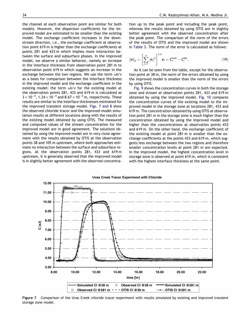
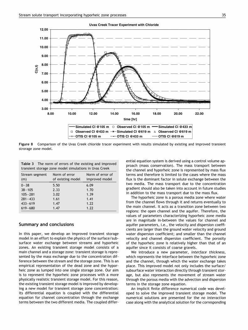
the channel at each observation point are similar for bothmodels. However, the dispersion coefficients for the im-proved model are estimated to be smaller than the existingmodel. The exchange coefficient increases in the down-stream direction, i.e., the exchange coefficient at observa-tion point 619 m is higher than the exchange coefficients atpoints 281 and 433 m which implies more interaction be-tween the surface and subsurface phases. In the improvedmodel, we observe a similar behavior, namely an increasein the interface thickness from observation point 281 m toobservation point 619 m which suggests an increase in theexchange between the two regions. We use the term aA/vas a basis for comparison between the interface thicknessin the improved model and the exchange coefficient in theexisting model: the term aA/v for the existing model atthe observation points 281, 433 and 619 m is calculated as3 · 10�4, 1.24 · 10�4 and 8.67 · 10�4 m, respectively. Theseresults are similar to the interface thicknesses estimated forthe improved transient storage model. Figs. 7 and 8 showthe observed chloride tracer and the improved model simu-lation results at different locations along with the results ofthe existing model obtained by using OTIS. The measuredand computed values of the stream concentration for theimproved model are in good agreement. The solutions ob-tained by using the improved model are in very close agree-ment with the results obtained by OTIS at the observationpoints 38 and 105 m upstream, where both approaches esti-mate no interaction between the surface and subsurface re-gions. At the observation points 281, 433 and 619 mupstream, it is generally observed that the improved modelis in slightly better agreement with the observed concentra-

Uvas Creek Tracer Exp

3.00

4.00

5.00

6.00

7.00

8.00

9.00

10.00

11.00

12.00

8.00 10.00 12.00 14.00

ti

C (

x,t)

Simulated Cl @38 m ObseObserved Cl @281 m OTIS

Figure 7 Comparison of the Uvas Creek chloride tracer experimstorage zone model.

tion up to the peak point and including the peak point,whereas the results obtained by using OTIS are in slightlybetter agreement with the observed concentration afterthe peak point. The comparison of the norm of the errorsof the results of OTIS and the improved model are shownin Table 3. The norm of the error is calculated as follows:

ek k2 ¼Xni¼1

eij j2" #1=2

ei ¼ Cnumi � Cobs

i . ð19Þ

As it can be seen from the table, except for the observa-tion point at 38 m, the norm of the errors obtained by usingthe improved model is smaller than the norm of the errorsby using OTIS.

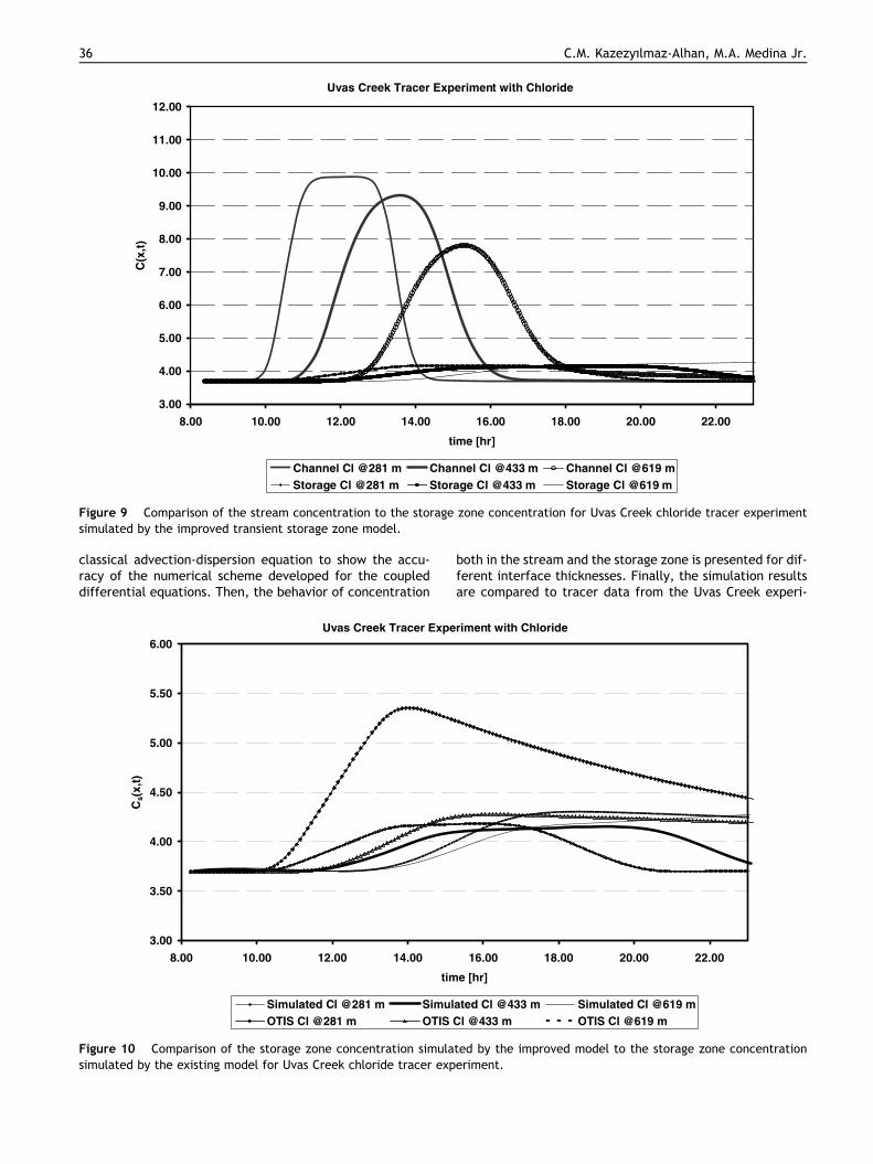
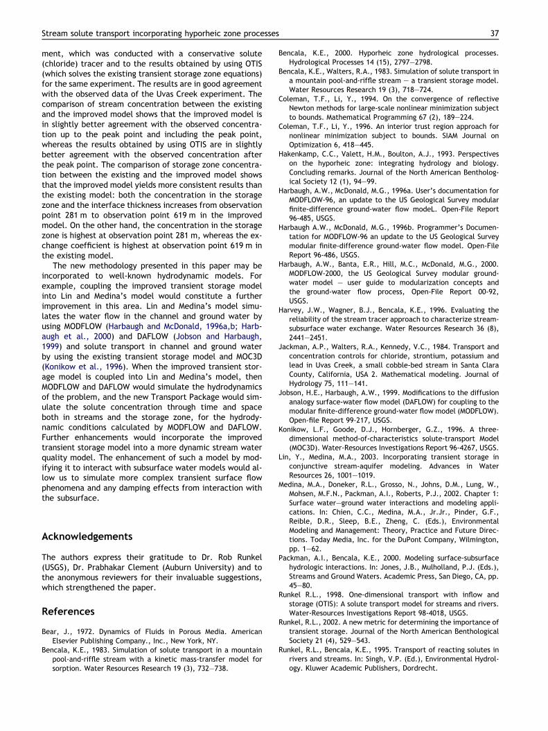
Fig. 9 shows the concentration curves in both the storagezone and stream at observation points 281, 433 and 619 mobtained by using the improved model. Fig. 10 comparesthe concentration curves of the existing model to the im-proved model in the storage zone at locations 281, 433 and619 m. The concentration obtained by using OTIS at observa-tion point 281 m in the storage zone is much higher than theconcentration obtained by using the improved model andhigher than the concentrations at observation points 433and 619 m. On the other hand, the exchange coefficient ofthe existing model at point 281 m is smaller than the ex-change coefficients at the points 433 and 619 m, which sug-gests less exchange between the two regions and thereforesmaller concentration levels at point 281 m are expected.In the improved model, the highest concentration level instorage zone is observed at point 619 m, which is consistentwith the highest interface thickness at the same point.

eriment with Chloride

16.00 18.00 20.00 22.00

me [hr]

rved Cl @38 m Simulated Cl @281 m Cl @38 m OTIS Cl @281 m

ent with results simulated by existing and improved transient

Uvas Creek Tracer Experiment with Chloride

3.00

4.00

5.00

6.00

7.00

8.00

9.00

10.00

11.00

12.00

8.00 10.00 12.00 14.00 16.00 18.00 20.00 22.00

time [hr]

C(x

,t)

Simulated Cl @105 m Observed Cl @105 m Simulated Cl @433 mObserved Cl @433 m Simulated Cl @619 m Observed Cl @619 mOTIS Cl @105 m OTIS Cl @433 m OTIS Cl @619 m

Figure 8 Comparison of the Uvas Creek chloride tracer experiment with results simulated by existing and improved transientstrorage zone model.

Table 3 The norm of errors of the existing and improvedtransient storage zone model simulations in Uvas Creek

Stream segment(m)

Norm of errorof existing model

Norm of error ofimproved model

0–38 5.50 6.0938–105 2.33 1.70105–281 3.02 1.39281–433 1.61 1.41433–619 1.47 1.22619–680 1.47 1.22


Summary and conclusions

In this paper, we develop an improved transient storagemodel in an effort to explain the physics of the surface/sub-surface water exchange between streams and hyporheiczones. An existing transient storage model consists of amain channel and a storage zone: transient storage is repre-sented by the mass exchange due to the concentration dif-ference between the stream and the storage zone. This is anempirical representation of the dead zone and the hypor-heic zone as lumped into one single storage zone. Our aimis to represent the hyporheic zone processes with a morephysically realistic transient storage model. For this reason,the existing transient storage model is improved by develop-ing a new model for transient storage zone concentration:its differential equation is coupled with the differentialequation for channel concentration through the exchangeterms between the two different media. The coupled differ-

ential equation system is derived using a control volume ap-proach (mass conservation). The mass transport betweenthe channel and hyporheic zone is represented by mass fluxterms and therefore is limited to the cases where the massflux is the dominant factor in solute exchange between thetwo media. The mass transport due to the concentrationgradient should also be taken into account in future studiesin addition to the mass transport due to the mass flux.

The hyporheic zone is a porous media zone where waterfrom the channel flows through it and returns eventually tothe main channel. It acts as a transition zone between tworegions: the open channel and the aquifer. Therefore, thevalues of parameters characterizing hyporheic zone mediaare in magnitude in-between the values for channel andaquifer parameters, i.e., the velocity and dispersion coeffi-cients are larger than the ground water velocity and groundwater dispersion coefficient; and smaller than the channelvelocity and channel dispersion coefficient. The porosityof the hyporheic zone is relatively higher than that of anaquifer since it consists of coarse gravels.

We introduce a new parameter, interface thickness,which represents the interface between the hyporheic zoneand the channel, through which the water exchange takesplace. This improved model not only includes the surface/subsurface water interaction directly through transient stor-age, but also represents the movement of stream waterthrough the porous media with the advection and dispersionterms in the storage zone equation.

An implicit finite difference numerical code was devel-oped to solve the improved transient storage model. Thenumerical solutions are presented for the no interactioncase along with the analytical solution for the corresponding

Uvas Creek Tracer Experiment with Chloride

3.00

4.00

5.00

6.00

7.00

8.00

9.00

10.00

11.00

12.00

8.00 10.00 12.00 14.00 16.00 18.00 20.00 22.00

time [hr]

C(x

,t)

Channel Cl @281 m Channel Cl @433 m Channel Cl @619 mStorage Cl @281 m Storage Cl @433 m Storage Cl @619 m

Figure 9 Comparison of the stream concentration to the storage zone concentration for Uvas Creek chloride tracer experimentsimulated by the improved transient storage zone model.


classical advection-dispersion equation to show the accu-racy of the numerical scheme developed for the coupleddifferential equations. Then, the behavior of concentration

Uvas Creek Tracer Expe

3.00

3.50

4.00

4.50

5.00

5.50

6.00

8.00 10.00 12.00 14.00

tim

Cs(

x,t)

Simulated Cl @281 m SimulOTIS Cl @281 m OTIS

Figure 10 Comparison of the storage zone concentration simulasimulated by the existing model for Uvas Creek chloride tracer exp

both in the stream and the storage zone is presented for dif-ferent interface thicknesses. Finally, the simulation resultsare compared to tracer data from the Uvas Creek experi-

riment with Chloride

16.00 18.00 20.00 22.00

e [hr]

ated Cl @433 m Simulated Cl @619 mCl @433 m OTIS Cl @619 m

ted by the improved model to the storage zone concentrationeriment.


ment, which was conducted with a conservative solute(chloride) tracer and to the results obtained by using OTIS(which solves the existing transient storage zone equations)for the same experiment. The results are in good agreementwith the observed data of the Uvas Creek experiment. Thecomparison of stream concentration between the existingand the improved model shows that the improved model isin slightly better agreement with the observed concentra-tion up to the peak point and including the peak point,whereas the results obtained by using OTIS are in slightlybetter agreement with the observed concentration afterthe peak point. The comparison of storage zone concentra-tion between the existing and the improved model showsthat the improved model yields more consistent results thanthe existing model: both the concentration in the storagezone and the interface thickness increases from observationpoint 281 m to observation point 619 m in the improvedmodel. On the other hand, the concentration in the storagezone is highest at observation point 281 m, whereas the ex-change coefficient is highest at observation point 619 m inthe existing model.

The new methodology presented in this paper may beincorporated to well-known hydrodynamic models. Forexample, coupling the improved transient storage modelinto Lin and Medina’s model would constitute a furtherimprovement in this area. Lin and Medina’s model simu-lates the water flow in the channel and ground water byusing MODFLOW (Harbaugh and McDonald, 1996a,b; Harb-augh et al., 2000) and DAFLOW (Jobson and Harbaugh,1999) and solute transport in channel and ground waterby using the existing transient storage model and MOC3D(Konikow et al., 1996). When the improved transient stor-age model is coupled into Lin and Medina’s model, thenMODFLOW and DAFLOW would simulate the hydrodynamicsof the problem, and the new Transport Package would sim-ulate the solute concentration through time and spaceboth in streams and the storage zone, for the hydrody-namic conditions calculated by MODFLOW and DAFLOW.Further enhancements would incorporate the improvedtransient storage model into a more dynamic stream waterquality model. The enhancement of such a model by mod-ifying it to interact with subsurface water models would al-low us to simulate more complex transient surface flowphenomena and any damping effects from interaction withthe subsurface.

Acknowledgements

The authors express their gratitude to Dr. Rob Runkel(USGS), Dr. Prabhakar Clement (Auburn University) and tothe anonymous reviewers for their invaluable suggestions,which strengthened the paper.

References

Bear, J., 1972. Dynamics of Fluids in Porous Media. AmericanElsevier Publishing Company., Inc., New York, NY.

Bencala, K.E., 1983. Simulation of solute transport in a mountainpool-and-riffle stream with a kinetic mass-transfer model forsorption. Water Resources Research 19 (3), 732–738.

Bencala, K.E., 2000. Hyporheic zone hydrological processes.Hydrological Processes 14 (15), 2797–2798.

Bencala, K.E., Walters, R.A., 1983. Simulation of solute transport ina mountain pool-and-riffle stream – a transient storage model.Water Resources Research 19 (3), 718–724.

Coleman, T.F., Li, Y., 1994. On the convergence of reflectiveNewton methods for large-scale nonlinear minimization subjectto bounds. Mathematical Programming 67 (2), 189–224.

Coleman, T.F., Li, Y., 1996. An interior trust region approach fornonlinear minimization subject to bounds. SIAM Journal onOptimization 6, 418–445.

Hakenkamp, C.C., Valett, H.M., Boulton, A.J., 1993. Perspectiveson the hyporheic zone: integrating hydrology and biology.Concluding remarks. Journal of the North American Bentholog-ical Society 12 (1), 94–99.

Harbaugh, A.W., McDonald, M.G., 1996a. User’s documentation forMODFLOW-96, an update to the US Geological Survey modularfinite-difference ground-water flow modeL. Open-File Report96-485, USGS.

Harbaugh A.W., McDonald, M.G., 1996b. Programmer’s Documen-tation for MODFLOW-96 an update to the US Geological Surveymodular finite-difference ground-water flow model. Open-FileReport 96-486, USGS.

Harbaugh, A.W., Banta, E.R., Hill, M.C., McDonald, M.G., 2000.MODFLOW-2000, the US Geological Survey modular ground-water model – user guide to modularization concepts andthe ground-water flow process, Open-File Report 00-92,USGS.

Harvey, J.W., Wagner, B.J., Bencala, K.E., 1996. Evaluating thereliability of the stream tracer approach to characterize stream-subsurface water exchange. Water Resources Research 36 (8),2441–2451.

Jackman, A.P., Walters, R.A., Kennedy, V.C., 1984. Transport andconcentration controls for chloride, strontium, potassium andlead in Uvas Creek, a small cobble-bed stream in Santa ClaraCounty, California, USA 2. Mathematical modeling. Journal ofHydrology 75, 111–141.

Jobson, H.E., Harbaugh, A.W., 1999. Modifications to the diffusionanalogy surface-water flow model (DAFLOW) for coupling to themodular finite-difference ground-water flow model (MODFLOW).Open-file Report 99-217, USGS.

Konikow, L.F., Goode, D.J., Hornberger, G.Z., 1996. A three-dimensional method-of-characteristics solute-transport Model(MOC3D). Water-Resources Investigations Report 96-4267, USGS.

Lin, Y., Medina, M.A., 2003. Incorporating transient storage inconjunctive stream-aquifer modeling. Advances in WaterResources 26, 1001–1019.

Medina, M.A., Doneker, R.L., Grosso, N., Johns, D.M., Lung, W.,Mohsen, M.F.N., Packman, A.I., Roberts, P.J., 2002. Chapter 1:Surface water–ground water interactions and modeling appli-cations. In: Chien, C.C., Medina, M.A., Jr.Jr., Pinder, G.F.,Reible, D.R., Sleep, B.E., Zheng, C. (Eds.), EnvironmentalModeling and Management: Theory, Practice and Future Direc-tions. Today Media, Inc. for the DuPont Company, Wilmington,pp. 1–62.

Packman, A.I., Bencala, K.E., 2000. Modeling surface-subsurfacehydrologic interactions. In: Jones, J.B., Mulholland, P.J. (Eds.),Streams and Ground Waters. Academic Press, San Diego, CA, pp.45–80.

Runkel R.L., 1998. One-dimensional transport with inflow andstorage (OTIS): A solute transport model for streams and rivers.Water-Resources Investigations Report 98-4018, USGS.

Runkel, R.L., 2002. A new metric for determining the importance oftransient storage. Journal of the North American BenthologicalSociety 21 (4), 529–543.

Runkel, R.L., Bencala, K.E., 1995. Transport of reacting solutes inrivers and streams. In: Singh, V.P. (Ed.), Environmental Hydrol-ogy. Kluwer Academic Publishers, Dordrecht.


Runkel, R.L., Chapra, S.C., 1993. An efficient numerical-solution ofthe transient storage equations for solute transport in smallstreams. Water Resources Research 29 (1), 211–215.

Runkel, R.L., Chapra, S.C., 1994. Reply. Water Resources Research30 (10), 2863–2865.

Runkel, R.L., McKnight, D.M., Andrews, E.D., 1998. Analysis oftransient storage subject to unsteady flow: diel flow variation inan Antarctic stream. Journal of the North American Bentholog-ical Society 17 (2), 143–154.

Runkel, R.L., McKnight, D.M., Rajaram,H., 2003. Modeling hyporheiczone processes. Advances in Water Resources 26 (9), 901–905.

Scott, D.T., Goosef, M.N., Bencala, K.E., Runkel, R.L., 2003.Automated calibration of a stream solute transport model:implications for interpretation of biogeochemical parameters.

Journal of the North American Benthological Society 22 (4),492–510.

The MathWorks., 2003. Optimization Toolbox for use with Matlab,User’s Guide, Version 2.

Wagner, B.J., Gorelick, S.M., 1986. A statistical methodology forestimating transport parameters: theory and applications toone-dimensional advective-dispersive systems. Water ResourcesResearch 22 (8), 1303–1315.

Winter, T.C., Harvey, J.W., Franke, O.L., Alley, W.M., 1998.Ground water and surface water as a single resource. USGeological Survey Circular 1139.

Worman, A., 1998. Analytical solution and timescale for transportof reacting solutes in rivers and streams. Water ResourcesResearch 34 (10), 2703–2716.

stream solute transport incorporating hyporheic zone processes

Documents