strength of materials - npteltextofvideo.nptel.ac.in/105105108/lec26.pdf · strength of materials ....

Strength of Materials Prof. S.K.Bhattacharya

Dept. of Civil Engineering, I.I.T., Kharagpur

Lecture No.26 Stresses in Beams-I

Welcome to the first lesson of the 6th module which is on Stresses in Beams part 1. In the

last module we had discussed some aspects of the shear force and bending moment on

beams and in this particular module we are going to discuss how to utilize the

information on the shear force and bending moment in evaluating the stresses in the

beam.

(Refer Slide Time: 01:04-01:05)

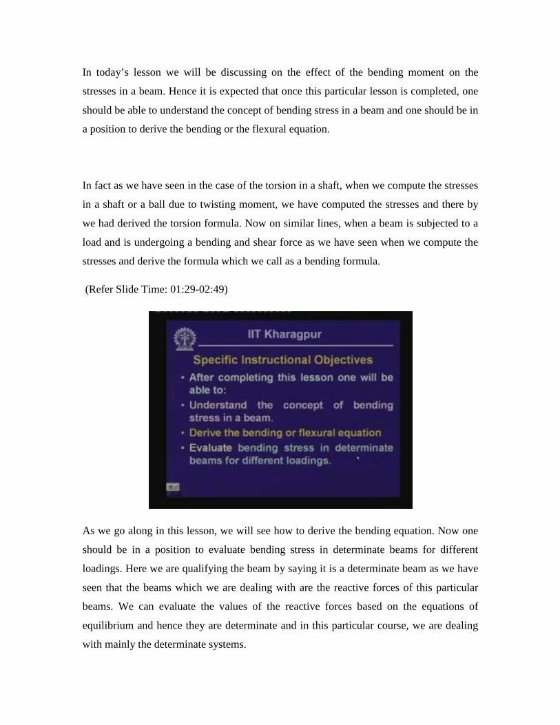
In today’s lesson we will be discussing on the effect of the bending moment on the

stresses in a beam. Hence it is expected that once this particular lesson is completed, one

should be able to understand the concept of bending stress in a beam and one should be in

a position to derive the bending or the flexural equation.

In fact as we have seen in the case of the torsion in a shaft, when we compute the stresses

in a shaft or a ball due to twisting moment, we have computed the stresses and there by

we had derived the torsion formula. Now on similar lines, when a beam is subjected to a

load and is undergoing a bending and shear force as we have seen when we compute the

stresses and derive the formula which we call as a bending formula.


As we go along in this lesson, we will see how to derive the bending equation. Now one

should be in a position to evaluate bending stress in determinate beams for different

loadings. Here we are qualifying the beam by saying it is a determinate beam as we have

seen that the beams which we are dealing with are the reactive forces of this particular

beams. We can evaluate the values of the reactive forces based on the equations of

equilibrium and hence they are determinate and in this particular course, we are dealing

with mainly the determinate systems.


Hence the scope of this particular lesson includes the recapitulation of the previous lesson

as we will be discussing the aspects of the previous lessons through the question answer

session. We will also be deriving the bending or the flexural equation in a beam due to

pure bending. In this particular lesson, we will discuss about the pure bending and then

we will looking into some examples for the evaluation of bending stresses in determinate

beams for different loadings.


Let us look into the questions which were given last time and their answers. The first

question given was on the effect of articulation in an indeterminate beam. Now this is a

term wherein we introduce a mechanism in a beam, where at that particular point it can

sustain the shear force but it cannot resist any bending moment. What happens if we

introduce this kind of articulation in a beam in an indeterminate beam? The next question

is that if we introduce a similar kind of articulation in a determinate beam then what will

be the consequence?


Let us look into these two questions in one go and let me answer those questions. If I

have a beam which is fixed at one end and subjected to different kinds of loading say

uniformly distributed load, concentrated load, a concentrated moment etc. Now as we

have seen in this particular beam at this end, we have a fixed support where we have

reactive forces such as the vertical force, the horizontal force and the bending moment.

This is the reactive force R, horizontal force H and moment M and all these 3 quantities

can be evaluated using the equations of statics namely the summation of horizontal forces

is 0, the summation of vertical forces is 0 and the summation of moment at any point

within this beam is 0. If we do that we can evaluate these unknown reactive forces H M

and R. So this particular system is a determinate system.

(Refer Slide Time: 05:23)

Let us supposing we introduce one roller at this particular end and thereby introduce

another reactive force in this particular end; (Refer Slide Time: 05:23) let us call this as

R1 and this as R2. Now as soon as we do this, this particular beam becomes indeterminate

that is it is no longer determinate. The reason is that we have 4 unknown reactions and

they are H, M, R1 and R2. So there are 4 unknown reactive forces and we have only 3

equations of statics. Hence this particular system is statically indeterminate.

To find a solution for such a problem, many a times we introduce another condition in a

beam. Let us say that we introduce a hinge in this particular beam inside and this hinge is

such that it cannot resist any moment but it can support shear force. It can support the

shear force at this particular end but it cannot resist any moment.

Now as soon as we introduce this particular kind of articulation in a beam wherein it

cannot resist any moment, that means we generate an additional equation from this

particular condition, that means if we take the moment of all the forces about that

particular point it is expected that the moment resistance will be 0.

Hence we get another equation based on which we can solve the unknown reactive

forces. If you have an articulation introduced in an indeterminate beam where you have

additional unknown reactive forces, then we can solve that or the beam becomes

determinate in that situation.

This particular articulation can be introduced in this form. This is the beam and the other

part may be resting on this in this particular form. So this particular part is fixed at this

end and this is on a roller. At this particular support if you split it into two parts the

reactive force from this particular part is supported on roller at this end now here we will

have a reactive force. These forces are the same and if we call this r this is also r because

this particular section can resist the shear force.

We can have a reactive force generator at this particular end. Now this is a determinate

system having a fixed end which is a cantilever and this is like a simply supported one

and these unknown reactive forces can be calculated which are the shear at this particular

end. If we have an articulation in a beam, then that indeterminate beam becomes a

determinate one. The beam becomes determinate because we generate an additional

equation so we have four unknowns.

We get three equations of statics and 1 additional equation, so it becomes a determinate

situation. Now if we have a determinate beam in which we do not have a support, it is

just a cantilever. Then if we have the cantilever beam which is fixed at this particular end

and let us suppose we introduce this articulation over here where again this is subjected

to different kinds of loading; distributed loading and the concentrated loading or may be a

concentrated moment.

If we have an articulation in this beam, that means if we have the beam again in the same

form as we were discussing that you have a fixed end here and this particular part is like

this. Since this particular part does not have any support, so when it is subjected to the

loading, it will topple because it cannot resist any moment over here. So, a determinate

beam becomes unstable when an articulation is provided in a determinate system.

This is the impact of the articulation. One should be careful that if you have an

indeterminate beam and if you introduce an articulation within the beam then that

indeterminate beam becomes determinate or you get an additional equation generated for

every articulation you induce and if you have a determinate beam in which we introduce

any articulation, it becomes unstable.


This is what is indicated over here where the introduction of articulation in an

indeterminate beam reduces the beam to a determinate one and the introduction of

articulation in a determinate beam reduces the beam to an unstable system.


So, that answers the first two questions. Now the third question is: What is the necessity

of drawing shear force and bending moment diagrams of beams? You have gone through

the previous module wherein we have discussed various kinds of loading on various

kinds of beams and then we have evaluated the shear forces and bending moment at

different sections.

If we need to know the variation of the shear force or the bending moment along the

length of the beam and if we draw the diagram over the length of the beam where the

variation of the shear force is at every section then it becomes easier to understand

‘which’ part of the beam is subjected to ‘what’ kind of shear forces or bending moment.

From the diagram of shear force or the bending moment readily, we can get the different

values of bending moments and shear force along the length of the beam from which we

can determine at which part the magnitude of the shear force of the bending moment is

larger or smaller. Hence, for evaluating the stresses in a beam it becomes much simpler.

Once we know the variation of the shear force and the bending moment in a beam, it

becomes easier to compute the corresponding stresses.


In this lesson we will discuss how that induces the bending stress in the beam. So, the

shear force and bending moment diagram indicate their variations respectively in a beam.

The variation of the bending moment and shear force along the length of the beam and

the diagram thus help in finding the maximum values of shear force or the bending

moment because when we deal with stresses, we will need the maximum magnitude of

the bending moment based on which we can compute the stress.

We need to know at which point for some loading in a beam the maximum bending

moment occurs and for that reason, we need to draw the bending moment diagram and so

is the case with the shear force.


Let us see what happens when a beam is subjected to a pure bending. We had drawn the

shear force and bending moment diagram for a beam say which is simply supported and

subjected to two concentrated loads which are placed equally from the two ends say

distance a and a and in this particular beam, we had drawn the bending moment diagram

wherein you had seen that the bending moment over this particular zone is constant.

If you have a cantilever beam in which you have a concentrated moment, you also get the

same moment ‘m’. So these are the cases where a beam is subjected to pure bending

moment. Now when a beam is subjected to this kind of pure bending moment, then if we

are interested in finding out the stresses, we need to develop the relationship between the

bending moment that is acting in the beam and the corresponding stress induced in the

section in terms of the sectional properties and that is what we are going to look into now.

As we made some assumption while deriving the torsion equation, we make some

assumptions here as well. Let us assume that this is a part of the prismatic beam in which

the cross section of this particular beam is such that it is symmetrical with respect to the

vertical axis y and so this is y axis. Now this particular section here is soon in the form of

a trapezium wherein this is symmetrical with respect to y axis where as it is not

symmetrical with respect to z axis since x is a longer length of the member.

This is the centroid of this particular section. The axis which we draw along the centroid

we call as the axis of the beam. Also along the y axis if we pass the plane the load acts

and the bending which is acting in the beam are in the vertical plane. Here we assume

that the section is symmetrical with respect to this vertical plane and the plane of bending

is this particular plane and also in this particular plane the load acts.

So we say generally that the beam has an axial plane of symmetry, which is the x y plane

in this particular case and this is the plane of symmetry. That means the section is

symmetrical with respect to this plane and the applied loads lie in the plane of symmetry

which is what we assume over here.

As we have seen that because of the loading it will be subjected to shear force and

bending moment it will undergo deformation. Now when it undergoes deformation the

axis of the beam which we have chosen over here undergoes bending and we assume that

it does not undergo stretching. The most important assumption which we make over here

is that the cross section of the beam which was plane before the application of the load

remains plane or perpendicular to the deformed axis after the bending occurs.

That means after the beam undergoes bending which forms a part of the circle and the

axis also takes that particular form of the circle and anywhere if we take a section the

cross section remains perpendicular to the deformed axis and the section which was plane

originally, remains plane even after bending. Thus this is one of the main assumptions

which you make while deriving the bending equation.


Now with these assumptions let us look into a small segment of this prismatic beam

wherein it is acted on by the pure moment M. Let us say that we take a small segment out

of this prismatic beam of length d x and we choose a fiber a and b and a b also is of

length d x. Let us assume that a b is at a distance of y from this axis of the beam which is

the x axis. Under loading let us say it under goes deformation and the deform shape is

something like this which is a part of a great circle.

Let us concentrate on this particular segment which was originally d x and let us say that

it undergoes deformation. Along this particular length this is d s and this axis of the beam

has a radius Row with reference to the center of this great circle. The fiber a b here is a

dash b dash and now here at a distance of y this also under goes deformation.

Let us assume that this particular segment forms an angle d Theta. Hence the radius of

this particular arc is Row– y. We can write this particular distance d s from the radius r

and this angle d theta as Row D Theta and we can write the segmental distance a dash b

dash as Row - y d Theta.

If we call this as d u bar, this is Row - y d Theta. The final length - the original length

which is Row d Theta is the deformation and we get - y d Theta. Let us divide this by the

original length and d u bar d s = - y d Theta d s and d s as you know is Row d Theta. So,

we get - y by Row. Now d u bar is the stretching in the curve direction and if we take its

horizontal component, the angle being very small causes that angle which varies. We can

call d u bar as the axial stretching d u.

Like wise the distance d s which is around the arc length has a component in the

horizontal direction which is equal to the original length dx. If we substitute that this

gives us the extension d u over the original length dx and as we have defined the

extension over the original length as a strain. We call the strain along the axial direction

or normal to the cross section as normal strength which is –y/Row.

If we call epsilon as the normal strength which -y by Row and Row is the radius of

curvature of the axis of the beam and many a times we designate this particular quantity

1/Row as Kappa which we call as curvature and the strength Epsilon is –y/Row.

Consequently, as we know the relationship between the stress and strain in terms of the

modulus of elasticity is Sigma = e multiplied by Epsilon. This is as per the hooks law

assuming that we are dealing with beams that are within their elastic limit.

So within the elastic limit stress is proportional to the strain as per the hooks law. The

stress Sigma is equal to e multiplied by epsilon and = -E (y)/Row. Here epsilon is equal to

–y/Row and Sigma = -E(y)/Row. These are the values of the normal strain and stress

which act on the cross section of the member. Here you note that strain in the stress vary

along the depth y which is the depth of the beam. From the geometrical compatibility of

the beam under the geometrical deformation we understand how it undergoes strain.

This gives us a relationship which we call as compatibility. We have to look into the

equations of equilibrium so that we can establish the relationship between the stress and

the corresponding stress resultant which is the moment. Let us keep this aspect in mind

that epsilon = -y by Row and Sigma = - e y / Ρ and we need to locate where the variation

of y is along the depth.


Now let us look into a segment of this beam again. We have shown three axis: the z axis,

the y axis and the x axis. Let us consider a small element here having an area d a. As we

know that the summation of the horizontal forces f x = 0 and this force is nothing but the

stress multiplied by the area. If we integrate these over the entire area this is 0. The

Sigma as we have seen is -E y /Row (da) integral this over area which is equal to 0.

If we take out these two constants, e - e Row e (Row) so this over area a y d a = 0. Now

we can write this as a y bar times this constant value e /Row = 0. Since area a ≠ 0 y bar =

0 which means that the distance of that segmental area with respect to the centroid axis or

origin is 0. This can happen only if the centroid of the cross section matches with the

origin.

Now this signifies that the z axis must pass through the centroid of the beam. If this y = 0

then from the expression of strain which we had as -y /Row and Sigma as - e y /Row

these quantities are 0 when y = 0. That means at this particular point the strain and the

stress is 0 and that is the reason this particular axis is termed as the neutral axis. In fact if

we look into the cross section we have a point where the strain and the stress is 0 and it

linearly varies in the entire depth of the beam.

We will have a variation wherein we will have a zero strain or zero stress over here and

here we will have strain and corresponding stresses and this will give us the variation of

the strain and the stress. This is one equation of equilibrium from which we can position

or locate the neutral axis in the cross section.

For positioning the neutral axis in the cross section it should pass through the centroid of

the cross section. Given a cross section which is symmetrical with respect to y axis we

got to locate its centroidal point and through the centroidal point the neutral axis will pass

through. This is the information which we get corresponding to this particular

equilibrium equation.

Let us look into the relationship between the moment and the stress. The other

equilibrium equation which we can have is the moment value. Let us take the moment of

this particular area where this is the beam segment which we are assuming with a

moment M and here we are considering the force which is Sigma x (da). So the moment

of this force is Sigma x d a multiplied by the distance y. If we call this distance as y then

moment M + Sigma x da(y) integrated over the area is 0.

If you substitute the value of Sigma this is m- e/Row (y d a y) = 0. This is nothing but M

= E /Row (integral y square) d a. This integral y square d a is the second moment of this

segmental area with reference to this neutral axis and this we designate as the moment

of inertia and we call this as I. From this relationship we get M = E I by Row. Now we

have already observed that in the relationship between the stress and the Row we have

Sigma = - E y by Row.


From these we can say that Sigma/y = E/Row. So, Sigma/y = - E/Row and E/Row = M

/E I so this - M/I. So, we can write that M/I = E/Row = - Sigma/y. This particular

equation which relates the moment with the curvature we call as the bending equation or

the moment equation. Finally this is the diagram which we get.

As we have seen that this is the plane of bending along which the load acts. We call this

particular axis along which the stress is 0 as neutral axis and for each cross section if we

plot this neutral axis, we get a surface which we call as neutral surface. The neutral

surface of the beam which is plotted over here is the axis of the beam and this is the

neutral axis of the cross section.


The bending equation which we get is this kind where the M is the bending moment, I is

the moment of inertia, E is the modulus of the velocity, Row is the radius of the curvature

of the neutral axis, Sigma is a stress and y is the point at the point where we are trying to

find out the bending stress.

Now in a beam at a particular cross section if our interest is to evaluate the bending

stress, the location of that particular point with reference to the neutral axis will be known

and hence the distance y will be known. Here ‘I’ is the moment of inertia of the cross

section with respect to the neutral axis and M is the bending moment which is acting at

that particular section. Once we know these parameters, we can compute the value

Sigma. So from these we can write that the relationship M/I = -Sigma/y or Sigma = M

y/I.

If we take a segment in the positive bending moment in the beam this particular type of

moment causes compression at the top and tension at the bottom because of the bending

which is acting in this particular segment. The bottom fibers undergo stretching which we

call as tensile and the top fiber undergoes compression which is compressive. If we apply

the positive bending moment in this particular equation we get the stress as negative and

the negative stress indicates that it is compression and likewise if we compute the stress

at the bottom fiber wherein y will be negative, we get the stress as positive and there by

the positive stress gives us the tensile stress.

If we take the positive moment and correspondingly if we place the values of y according

to the position of the point where we are evaluating the stress, the negative value of the

stress will give us the compressive stress and the positive value will give us a tensile

stress. These are the steps that we must go through to find out the bending stress at a

point in a given cross section.


When we want to find out the stress at that particular section, we must know what is the

value of the bending moment it is subjected to because of the external load that is acting

on the beam. So for a particular type of a beam for which we know the support condition

and the loading on the beam, we compute the value of the bending moment at a particular

section where we want to evaluate the bending stress.

Once we know the value of the bending moment then for that particular cross section we

have to establish the position of the neutral axis and once you know the neutral axis, you

can compute the moment of inertia of that particular section and also distance y with

respect to the neutral axis and we know the bending moment.

We know the distance y, we know the moment of inertia of the cross section with respect

to the neutral axis, so we can compute the value of the bending stress which is M y/I and

this is what is indicated over here. You have to evaluate the bending moment at the point

where you want to find out the stress and locate the position of the neutral axis. You will

have to determine the moment of inertia of the cross section about neutral axis and you

will have to determine the y coordinate of the point so that you know the distance y.

The position of the neutral axis will guide us to evaluate ‘I’ and y. These two parameters

will be dependent on this and then we will have to compute the bending stress from this

expression which is M y/I. We can take the appropriate sign of the corresponding

parameter so that the stress can be completed. We can then conclude whether there is a

compressive stress or tensile stress that is acting at that particular point. That is how you

can visualize how the variation of the bending moment or shear force along the length of

beam is going to help us evaluate the stress at a point in a beam which is subjected to

some kinds of loading.


Let us take some examples wherein we can apply this technique. Now this is the example

problem which in fact I had given you last time and asked you to solve. We need to draw

the shear force and bending moment diagram for this particular beam and as you can see

here, this is on hinged support and this is on a roller support and there is an over hand on

this beam and this is subjected to a uniformly distributed load of 10 kilo Newton/m.

Here the reactive forces will have a vertical reaction RA and we will have the horizontal

reaction HA and here we will have the vertical reaction RB. Since we do not have any

horizontal load on this, the summation of horizontal force = 0 will give us the reactive

force HA = 0. Now the summation of vertical force = 0 means RA + RB = the total force

which is 10 kilo Newton/m over a length of 3M and this is 30 kilo Newton.

If we take the moment of all the forces with respect to a beam, then we can get the value

of the reactive force R. So, RA (2), which is a clockwise moment and this loading, causes

an anti-clockwise moment and this part of the loading causes a clockwise moment. So,

RA (2) + this part is 10(1) (1/2) which is a moment over this point and this part is -10(2)

(1) = 0. So, this is 10(220) and this is 5 and we get -15. Here RA = 7.5 kilo Newton and

correspondingly from this RB = 30 kilo Newton.

Let us look into some examples wherein we can draw the shear force and the bending

moment diagram. Here RA + RB = 30 kilo Newton and RA = 7.5 kilo Newton and RB =

22.5 kilo Newton. Now let us take a section here at a distance of x so that we can draw

the free body of that particular part and if we draw the free body of that part we get the

reactive force R A.


Here, we have the shear force V, the bending moment M, the uniformly distributed load

which is acting over this particular segment and the length of this segment which is x. If

we take the equilibrium of the vertical forces, then we have V + RA - 10(x) = 0. This

gives us V = 10 x-RA and R A = 7.5 and we get the expression V=10x - 7.5.

Correspondingly, if we calculate the value of the bending moment, we have a bending

moment M acting in an anticlockwise direction. The load gives a moment in an anti-

clockwise direction if we take the moment with respect to this point, so M + 10. This is x

and this distance is x/2 so x square/2 - RA (x) = 0.This gives us M = 7.5(x) = 5x square

which is the expression for the bending moment and we have the values of the bending

moment and the shear force indicated by this expression.

If we need to find out the shear force at the point B where x = 2 since we do not have any

load in between at x = 2, the value of V = 10 (-7.5) = 20 -7.5 and this is 12.5 and this is +

12.5. When x = 0, V = -7.5 and V at x = 2 and V = +12.5. It varies from -7.5 to 12.5 and

somewhere in between, the shear force will be 0.

Let us suppose we need to know the point where the shear force is 0. Since we know

this is the expression for the shear force between A and B; we substitute V = 0 so 0 = 10x

-7.5 which gives us the value of x which =0.75. At a distance of 0.75 from the left end,

the value of the shear force is 0 which is indicated over here. At the point of the shear

force where the value is 0 the sign changes from the positive to the negative or vice versa

and these are the places where you can expect that the bending moment is going to be 0.

Here, this is one of the places where it is expected that the bending moment could be

maximum. Now corresponding to the slope from 7.5 to 12.5, we get over here if you look

into a section corresponding to this beyond this reactive value, what would be the value

of the shear force that we get? We have RA here, we have RB here and we have the

uniformly distributed load. Now this is the section which is at a distance of x from here

and we have the section which is V and the moment M so V + RA + RB - 10 (x) = 0.

So, the shear force V = 10x - RA - RB. Here x is 2; so this is 20 - 7.5 = 12.5 an RA= 12.5

and RB is 22.5 and this is 10. We get a positive value of shear as 10 and from 12.5 to - 10

it will become 0. This is the variation of the shear force and this is the shear force

diagram for this particular beam.

Consequently, let us look at the value of the bending moment where x = 0 and the

moment = 0. Now when x = .75, we get a value of bending moment which = 2.813 kilo

Newton meter. If we substitute the value of x = .75, we get the value of the maximum

positive bending moment. When we compute the bending moment at this particular point

when x = 2, we find that this is 15 - 4 (5) = 20 and this is 15. This gives us a -5 kilo

Newton meter and at this point, we get a bending moment which is 5 kilo Newton meter

which is negative.

In a beam as we have discussed earlier you can get the values positive in the maximum

value at a different point but if we are interested in the maximum possible values, then

whether it is negative or positive, the maximum bending moment that is occurring in this

particular section or in this particular beam is 5 kilo Newton meter.

The maximum positive bending moment is 2.813 kilo Newton meter and we get the

variation of the bending moment and the variation of the shear force. If you notice here

that the bending moment diagram also changes its signs from positive to negative so

somewhere within this particular zone A B, the bending moment = 0.

Let us suppose we want to compute the distance that you can compute from this bending

moment diagram, bending moment expression. Here we have the expression for the

bending moment as m = 7.5x - 5x square. Now if this moment is 0, we have 7.5x = 5x

square. So, if we say x = 1.5M at a distance of 1.5M the bending moment = 0 and this

distance is 1.5M from here.

So, the magnitude of the bending moment at this point which is at this support point = 5

kilo Newton meter because of this overhand and the bending moment is 0 at a distance of

1.5M from the left support and we get the values of the bending moment and shear force

for this particular problem.


Now let us look at another example that I had given you last time wherein in these

particular beams, we have introduced an articulation and let us look into this particular

beam which is of indeterminate type this beam which is on hinge support and this on one

roller support. If you look into the reactive forces here we have the vertical force here, we

have the horizontal force here and we have RB, this is RC and this is RE.

Now here you have a horizontal force HA and take a look at the number of unknowns 1,

2, 3, 4 and as we have seen that we have three equations of statics and four unknown

reactive values. Hence we cannot solve it using equations of statics alone which is why it

is an example of an indeterminate beam. Now since we have one additional unknown

equation to be evaluated we need at least another equation so that we can solve for the

unknown reactive forces.

This additional equation can be generated from the criteria that it has been indicated. The

beam has an articulation wherein these articulations can take the shear but cannot resist

the bending moment. It will take the moment of all the forces with respect to this

particular point which is 0 and then we get an additional set of equations. Basically here

there are two beams which are interconnected at this particular part. So if we compute the

values of the reactive forces, then we can evaluate the shear force diagram based on

which we can find out the maximum shear force in the beam.


We have the diagram plotted but this particular beam has been split at the articulation and

we have introduced one reactive force RD over here. Now these two forces are balancing

in nature, which means that one beam is getting supported over the other and transferring

the shear force here. It can resist the shear force but it rotates when it comes for the

bending.

If we are interested in finding out the values of this uniformly distributed load acting over

q, we have a length 2L and all these segmental lengths or L and the summation of

horizontal force 0 which gives you 0. Let us take this particular part RD + RE = 2q Lq

(L). So, we have one equation and from this we can say that if we take the moment of RD

with respect to this point then RE (2L) = q (2L) (L). So, 2L gets cancelled and RE = q (L)

and there by RD = q (L). The values of the reactive forces are RE and RD = q (L).

In the left segment the summation of vertical forces 0 will give you RB + RC - RD + P =

0. So this gives us RB + RC = RD -P and RD = qL and we have qL - P. If you take the

moment of all the forces with respect to this, then we get another set of equations for RB

and RC and correspondingly we get the value of RB = -2P - qL and the value of RC.

Correspondingly, we get 2qL + P and we get the values of reactive forces where RE = qL

and the shear force which acts in the articulation as RD = qL.

Now if we plot the shear force and take a free body over here, we have the force P and

this is V. So, P + V = 0 and V = -P and here we have -P from here to here. Since you do

not have any other load, at this particular point if you take the free body we have the

force which is acting over there which is P and we have the reactive force RB. So, we

have P, RB and V here and we have V + P + RV = 0. Therefore V = -P -RB and RB = -2P

- qL. So, this is +2P + q L and that will give us a value of P + q L.

Here we get a shear force of magnitude P + qL and from -P it changes over to + P + qL.

Then up to this segment again, the situation is the same and everywhere we have the

identical shear force. Now immediately after this particular reactive force if you take the

free body diagram of this particular part we have P + RB + RC + P = 0 and from there if

we compute the value of V we find that it becomes again -qL.

Up to this it is uniform since we do not have any load in between from qL. Here it varies

over the length of 2i 2L and -qL to + q L and comes back over here. So this is the

variation of the shear force over the entire length of the beam. If we note that this is the

maximum value of the shear force that we get anywhere within this here it is P, here it is

qL, here it is P + qL, the maximum value of the shear force is P + qL which occurs just

after this particular reactive force V which is what was asked for in this particular

example.


Now let us look an example which is based on our discussion. In this particular beam let

us call this as A B and this beam has a rectangular cross section of size 50mm/80mm.

We will have to determine the magnitude and location of the maximum bending stress in

the beam. First we will have to find out the magnitude and also we will have to locate

where this maximum stress is occurring and this is subjected to a concentrated load 2 kilo

Newton and a concentrated moment 5 kilo Newton meter.

To evaluate the value of bending stress at a point, we need to know the bending moment

that is acting at that particular section. So, first we need to draw the shear force and the

bending moment diagram of this particular beam. Since we have a hinged support and a

roller support we have a reactive force which is a vertical reaction RA and the horizontal

reaction HA and we have the vertical reactive force RB over here.

If we take the summation of horizontal forces as 0, HA = 0 and the summation of vertical

forces will give RA + RB = 2 and if we take the moment about this particular point of all

the forces we get the values of RA. So let us compute first the reactive forces and then

plot the shear force diagram so that we can compute the position of the maximum

bending moment and the bending stress.


This is the reactive force RA, the horizontal force HA and the vertical reactive force. Here

we have RB over the beam segment A B. Now the moment about B= 0 gives us RA (3)

which is a clockwise moment and class 5 kilo Newton meter which is also a clockwise

moment and 2 kilo Newton meter which is an anticlockwise moment and we get 0. We

get a value of RA = -1 kilo Newton and as we have seen i= 2kilo Newton and RA -1 kilo

Newton will give us the value of RB = 3 kilo Newton.

These are the values of RA and RB. Now take a section over here which has a reactive

force which is 1 kilo Newton and this being negative is in the opposite direction and we

have a positive value of the shear and the moment does not change the vertical force.

You have the uniform shear which is of +1 kilo Newton. At the load point there is a

change over from -1 + 1-3. So this is a 3 kilo Newton load which is shear and then finally

it is constant over this particular region. So, we get the value which is the shear force

diagram. If you plot the bending moment diagram correspondingly, we find that at the

point of the concentrated moment from 1 kilo Newton, it changes over to 4 kilo Newton

meter and here the moment comes to 3 kilo Newton meter and we get 0.

As we can see the value of the maximum bending moment is 4 kilo Newton meter and if

we compute the bending stress c= My (Ic) = M y (I). Here M = 4 kilo Newton meter

which is 4(10 to the power of 6) y = 50 y = 80y= 40 and this is 50 × 80q/12. The stress is

75 Mega Pascal and this bending stress here is a positive value which is why we will

have compression at the top and tensile stress at the bottom. The bending causes a

bending stress of 75 mpa which is located just to the right of the concentrated moment

and we have a negative magnitude which is a compressive stress at the top and a tensile

stress at the bottom.

We have another problem wherein we have a uniformly distributed load and a

concentrated load on a simply supported beam. We will have to determine the largest

allowable value of P if the bending stress is limited to 10 Mega Pascal. This problem is

set for you, which we will discuss in the next lesson.

(Refer Slide Time: 56:42 - 57:00)


Let us summarize this particular lesson. We have included what we have looked into in

the previous lesson; we have introduced the concept of the bending stress and we have

derived the bending equation and also looked into some examples to evaluate the bending

stresses in a beam.

(Refer Slide Time: 57:20 – 57:30)

Now these are the following questions given for you:

What are the assumptions made in evaluating the bending stress in a beam? What is the

bending equation? How do you locate neutral axis in a given cross section of a beam? We

will answer these questions in the next lesson.

strength of materials - npteltextofvideo.nptel.ac.in/105105108/lec26.pdf · strength of materials ....

Documents