strengths and limitations of adjustment … · in medical research logistic regression and cox...

CHAPTER 3

STRENGTHS AND LIMITATIONS OFADJUSTMENT METHODS

3.1 “CONDITIONING ON THE PROPENSITY SCORE

CAN RESULT IN BIASED ESTIMATION OF

COMMON MEASURES OF TREATMENT EFFECT:A MONTE CARLO STUDY”

Edwin P. Martensa,b, Wiebe R. Pestmanb and Olaf H. Klungela

a Department of Pharmacoepidemiology and Pharmacotherapy, Utrecht Institute of PharmaceuticalSciences (UIPS), Utrecht University, Utrecht, the Netherlandsb Centre for Biostatistics, Utrecht University, Utrecht, the Netherlands

Statistics in Medicine 2007, 26;16:3208-3210

Letter to the editor as reaction on: Austin PC, Grootendorst P, Sharon-Lise TN, Anderson GM.Conditioning on the propensity score can result in biased estimation of common measures oftreatment effect: A Monte Carlo study. Statistics in Medicine 2007, 26;4:754-768, 2007

33

CHAPTER 3: STRENGTHS AND LIMITATIONS OF ADJUSTMENT METHODS

ABSTRACT

In medical research logistic regression and Cox proportional hazards regression analysis, inwhich all the confounders are included as covariates, are often used to estimate an adjustedtreatment effect in observational studies. In the last decade the method of propensity scores hasbeen developed as an alternative adjustment method and many examples of applications can befound in the literature. Frequently this analysis is used as a comparison for the results foundby the logistic regression or Cox proportional hazards regression analysis, but researchers areinsufficiently aware of the different types of treatment effects that are estimated by these anal-yses.

This is emphasized by a recent simulation study by Austin et al. in which the main objec-tive was to investigate the ability of propensity score methods to estimate conditional treatmenteffects as estimated by logistic regression analysis. Propensity score methods are in generalincapable of estimating conditional effects, because their aim is to estimate marginal effectslike in randomized studies. Although the conclusion of the authors is correct, it can be easilymisinterpreted. We argue that in treatment effect studies most researchers are interested in themarginal treatment effect and the many possible conditional effects in logistic regression anal-ysis can be a serious overestimation of this marginal effect.

For studies in which the outcome variable is dichotomous we conclude that the treatmenteffect estimate from propensity scores is in general closer to the treatment effect that is of mostinterest in treatment effect studies.

Keywords: Confounding; Propensity scores; Logistic regression analysis; Marginal treatmenteffect; Conditional treatment effect; Average treatment effect

34 E.P. MARTENS - METHODS TO ADJUST FOR CONFOUNDING

3.1 BIASED ESTIMATION WITH PROPENSITY SCORE METHODS?

In a recent simulation study Austin et al. conclude that conditioning on the propensity scoregives biased estimates of the true conditional odds ratio of treatment effect in logistic regressionanalysis. Although we generally agree with this conclusion, it can be easily misinterpreted be-cause of the word bias. From the same study one can similarly conclude that logistic regressionanalysis will give a biased estimate of the treatment effect that is estimated in a propensity scoreanalysis. Because propensity score methods aim at estimating a marginal treatment effect, webelieve that the last statement is more meaningful.

DIFFERENT TREATMENT EFFECTS

The authors raise an important issue, which is probably unknown to many researchers, that inlogistic regression analysis a summary measure of conditional treatment effects will in gen-eral not be equal to the marginal treatment effect. This phenomenon is also known as non-collapsibility of the odds ratio,1 but is apparent in all non-linear regression models and gener-alized linear models with a link function other than the identity link (linear models) or log-linkfunction.2 In other words, even if a prognostic factor is equally spread over treatment groups,the inclusion of this variable in a logistic regression model will increase the estimated treatmenteffect. This increasing effect of a conditional treatment effect compared to the overall marginaleffect is larger when more prognostic factors are added, but lower when the treatment effect iscloser to OR=1 and also lower when the incidence rate of the outcome is smaller.3 In general, itcan be concluded that in a given research situation many different conditional treatment effectsexist, depending on the number of prognostic factors in the model.

TRUE CONDITIONAL TREATMENT EFFECT

The true treatment effect is the effect on a specific outcome of treating a certain populationcompared to not treating this population. In randomized studies this can be estimated as theeffect of the treated group compared to the non-treated group. The true conditional treatmenteffect as defined in Austin et al. is the treatment effect in a certain population given the set ofsix prognostic factors and given that the relationships in the population can be captured by alogistic regression model. Two of the six prognostic factors were equally distributed betweentreatment groups and included in the equation for generating the data. But there are also non-confounding prognostic factors excluded from this equation, because not all of the variationin the outcome is captured by the six prognostic factors. That means that it seems to be atleast arbitrary how many and which of the non-confounding prognostic factors were includedor excluded to come to a ‘true conditional treatment effect’. Because of the non-collapsibilityof the odds ratio, all these conditional treatment effects are in general different from eachother, but which of these is the one of interest remains unclear. The only thing that is clear,

E.P. MARTENS - METHODS TO ADJUST FOR CONFOUNDING 35


is that application of the model that was used to generate the data will find on average this‘true conditional treatment effect’, while all other models, including less or more prognosticfactors, will in general find a ‘biased’ treatment effect. It should be therefore no surprise thatpropensity score models will produce on average attenuated treatment effects, for propensityscore models correct for only one prognostic factor, the propensity score. This implies that thetreatment effect estimates from propensity score models are in principal closer to the overallmarginal treatment effect than to one of the many possible conditional treatment effects.

MARGINAL OR CONDITIONAL TREATMENT EFFECTS?

The authors give two motivations why a conditional treatment effect is more interesting thanthe overall marginal treatment effect (which is the effect that would be found if treatmentswere randomized). Firstly, they indicate that a conditional treatment effect is more interest-ing to physicians, because it allows physicians to make appropriate treatment effect decisionsfor specific patients. Indeed, in clinical practice treatment decisions are made for individualpatients, but these decisions are better informed by subgroup analyses with specific treatmenteffects for subgroups: a specific conditional treatment effect is still some kind of ‘average’ overall treatment effects in subgroups. Another argument is that treatment decisions on individualpatients should be based on the absolute risk reduction and not on odds ratios or relative risks.4

Secondly, the authors suggest that in practice researchers use propensity scores for estimatingconditional treatment effects. However, in most studies in which propensity scores and logisticregression analysis are both performed, researchers rather have an overall marginal treatmenteffect in mind than one specific conditional treatment effect.5 Furthermore, the overall marginaltreatment effect is one well-defined treatment effect, whereas conditional treatment effects areeffects that are dependent on the chosen model. The reason for comparing propensity scoremethods with logistic regression analysis is probably not because the aim is to estimate con-ditional effects, but simply because logistic regression is the standard way of estimating anadjusted treatment effect with a dichotomous outcome.

In conclusion, propensity score methods aim to estimate a marginal effect, which in generalis not a good estimate of a conditional effect in logistic regression analysis because of the non-collapsibility of the odds ratio. An overall marginal treatment effect is better defined and seemsto be of more interest than all possible conditional treatment effects. Finally, these conditionaleffects are dependent on the number of non-confounders, which is not the case for propensityscore methods.


3.1 BIASED ESTIMATION WITH PROPENSITY SCORE METHODS?

REFERENCES

[1] Greenland S, Robins MR, Pearl J. Confounding and collapsibility in causal inference. Stat Science, 14:29–46,1999.

[2] Gail MH, Wieand S, Piantadosi S. Biased estimates of treatment effect in randomized experiments with non-linear regressions and omitted covariates. Biometrika, 71:431444, 1984.

[3] Rosenbaum PR. Propensity score. In: Armitage P, Colton T, eds. Encyclopedia of biostatistics. Wiley, Chich-ester, United Kingdom, 1998.

[4] Rothwell PM, Mehta Z, Howard SC, Gutnikov SA, Warlow CP. From subgroups to individuals: generalprinciples and the example of carotid endarterectomy. The Lancet, 365 (9455):256–265, 2005.

[5] Shah BR, Laupacis A, Hux JE, Austin PC. Propensity score methods gave similar results to traditional regres-sion modeling in observational studies: a systematic review. J Clin Epidemiol, 58:550–559, 2005.


3.2 AN IMPORTANT ADVANTAGE OF PROPENSITY

SCORE METHODS COMPARED TO LOGISTIC

REGRESSION ANALYSIS

Edwin P. Martensa,b, Wiebe R. Pestmanb, Anthonius de Boera, Svetlana V. Belitsera

and Olaf H. Klungela


Provisionally accepted by International Journal of Epidemiology

39


ABSTRACT

In medical research propensity score (PS) methods are used to estimate a treatment effect inobservational studies. Although advantages for these methods are frequently mentioned in theliterature, it has been concluded from literature studies that treatment effect estimates are sim-ilar when compared with multivariable logistic regression (LReg) or Cox proportional hazardsregression. In this study we demonstrate that the difference in treatment effect estimates be-tween LReg and PS methods is systematic and can be substantial, especially when the numberof prognostic factors is more than 5, the treatment effect is larger than an odds ratio of 1.25(or smaller than 0.8) or the incidence proportion is between 0.05 and 0.95. We conclude thatPS methods in general result in treatment effect estimates that are closer to the true averagetreatment effect than a logistic regression model in which all confounders are modeled. This isan important advantage of PS methods that has been frequently overlooked by analysts in theliterature.

Keywords: Confounding; Propensity scores; Logistic regression analysis; Marginal treatmenteffect; Conditional treatment effect; Average treatment effect


3.2 AN IMPORTANT ADVANTAGE OF PROPENSITY SCORES

INTRODUCTION

A commonly used statistical method in observational studies that adjusts for confounding, isthe method of propensity scores (PS).1, 2 This method focusses on the balance of covariatesbetween treatment groups before relating treatment to outcome. In contrast, classical methodslike linear regression, logistic regression (LReg) or Cox proportional hazards regression (CoxPH) directly relate outcome to treatment and covariates by a multivariable model. Advantagesto use PS methods that are frequently mentioned in the literature are the ability to include moreconfounders, the better adjustment for confounding when the number of events is low and theavailability of information on the overlap of covariate distributions.1–7 In two recent literaturestudies it is concluded that treatment effects estimated by both PS methods and regressiontechniques are in general fairly similar to each other.8, 9 Instead of a focus on the similarityin treatment effects between both methods, we will illustrate that the differences between PSmethods and LReg analysis are systematic and can be substantial. We will also demonstrate thattreatment effect estimates from PS methods are in general closer to the true average treatmenteffect than from LReg, which results in an important advantage of PS methods over LReg.

SYSTEMATIC DIFFERENCES BETWEEN TREATMENT EFFECT

ESTIMATES

In the literature review of Shah et al. the main conclusion was that propensity score methodsresulted in similar treatment effects compared to traditional regression modeling.8 This wasbased on the agreement that existed between the significance of treatment effect in PS methodscompared to LReg or Cox PH methods in 78 reported analyses. This agreement was denotedas excellent (κ = 0.79) and the mean difference in treatment effect was quantified as 6.4%. Inthe review of Sturmer et al. it was also stressed that PS methods did not result in substantiallydifferent treatment effect estimates compared to LReg or Cox PH methods.9 They reported thatin only 9 out of 69 studies (13%) the effect estimate differed by more than 20%.

The results of these reviews can also be interpreted differently: the dissimilarity betweenmethods is systematic resulting in treatment effect estimates that are on average stronger inLReg and Cox PH analysis. In Shah et al. the disagreement between methods was in thesame direction: all 8 studies that disagreed resulted in a significant effect in LReg or Cox PHmethods and a non-significant effect in PS methods (p = 0.008, McNemar’s test). Similarly,the treatment effect in PS methods was more often closer to unity than in LReg or Cox PH (34versus 15 times, p = 0.009, binomial test with π0 = 0.5). In the review of Sturmer et al. itturned out that substantial differences between both methods only existed when the estimatesin LReg or Cox PH were larger than in PS methods. Because both reviews were partly basedon the same studies, we summarized the results in Table 3.1 by taking into account studies that



were mentioned in both reviews. We included all studies that reported treatment effects for PSmethods (matching, stratification or covariate adjustment) and regression methods (LReg orCox PH), even when the information was that effects were ‘similar’.

Table 3.1: Comparison of treatment effect estimates between propensity score methods (PS) andlogistic regression (LReg) or Cox proportional hazards regression (Cox PH)8, 9

number of studies percentageTreatment effect is stronger in PS methods 24 25.0%Treatment effects are equal or reported as ‘similar’ 22 22.9%Treatment effect is stronger in LReg or Cox PH 50 52.1%

From all 96 studies (Table 3.1) there were twice as many studies in which the treatment effectfrom LReg or Cox PH methods was stronger than from PS methods: 50 versus 24 (= 68%).Testing the null hypothesis of equal proportions (binomial test, π0 = 0.5, leaving out the cate-gory when effects were reported to be equal or similar) resulted in highly significant differences(p = 0.003). The mean difference in the logarithm of treatment effects (δ)8 between both meth-ods was calculated at 5.0%, significantly different from 0 (p = 0.001, 95% confidence interval(CI): 2.0, 7.9). In studies with treatment effects larger than an odds ratio (OR) of 2.0 or smallerthan 0.5 this mean difference was even larger: δ = 19.0%, 95% CI: 10.3, 27.6.

We conclude that PS methods result in treatment effects that are significantly closer to thenull hypothesis of no effect than LReg or Cox PH methods. The larger the treatment effects,the larger the differences.

EXPLAINING DIFFERENCES IN TREATMENT EFFECT ESTIMATES

The reason for the systematic differences between treatment effect estimates from PS meth-ods and LReg or Cox PH methods can be found in the non-collapsibility of the odds ratio andhazard ratio used as treatment effect estimators. In the literature this phenomenon has beenrecognized and described by many authors.10–18 To understand this, we start by defining a trueaverage treatment effect as the effect of treating a certain population instead of not treating asimilar population, where similarity is defined in terms of prognostic factors. In general, this isthe treatment effect in which we are primarily interested and equals the average effect in ran-domized studies. Note that this treatment effect is defined without using any outcome modelwith covariates. When treated and untreated populations are similar on prognostic factors, thistrue average treatment effect can be simply estimated by an unadjusted treatment effect, forinstance a difference in means, a risk ratio or an odds ratio. When on the other hand bothpopulations are not similar on prognostic factors, as is to be expected in observational studies,one should estimate an adjusted treatment effect, trying to correct for all potential confounders.This can be done for instance by any multivariable regression model or by PS methods usingstratification, matching or covariate adjustment. When treated and untreated populations are



exactly similar on all covariates, unadjusted and adjusted treatment effects should coincide,because the primary objective of adjustment is to adjust for dissimilarities in covariate distri-butions: if there are none, ideally adjustment should have no effect. Unfortunately, this is notgenerally true, for instance when odds ratios from LReg analysis are used to quantify treatmenteffects. Consider two LReg models:

logit(y) = α1 + βtt (3.1)

logit(y) = α2 + β∗t t + β1x1 (3.2)

where y is a dichotomous outcome, t a dichotomous treatment, x1 a dichotomous prognosticfactor and α1 and α2 constants, eβt the unadjusted treatment effect, eβ∗t the adjusted treatmenteffect and eβ1 the effect of x1.

Suppose that in a certain situation only one prognostic factor exists (x1) with a differentdistribution for both treatment groups. An adjusted treatment effect β∗t will be interpreted asan estimate for the true average treatment effect, i.e. the effect that would be found when bothtreatment groups had similar distributions of x1. But when in reality the distribution of x1

is similar for both treatment groups and model 3.2 is applied, it turns out that the adjustedtreatment effect estimate β∗t does not equal the unadjusted treatment effect βt. More gener-ally, when both treatment groups are similar with respect to their covariate distributions, theadjusted and unadjusted treatment effects will not coincide in non-linear regression models orgeneralized linear models with another link function than the identity link (equalling a linearregression analysis) or log-link. We refer to the literature for a mathematical explanation of thisphenomenon10, 11, 19 and will illustrate in the next paragraph its implications for the comparisonbetween LReg and PS methods in epidemiological research.

ADJUSTING FOR EQUALLY DISTRIBUTED PROGNOSTIC FACTORS

To illustrate the non-collapsibility of the OR, we created a large population of n = 100, 000,a binary outcome y (πy varying from 0.02 to 0.20), a treatment t (πt = 0.50) and 20 binaryprognostic factors x1, ..., x20 with πx1= ... =πx20 = 0.50 and eβx1= ... =eβx20 = 2.0.These factors, which we will call non-confounders, were exactly equally distributed acrosstreatments t = 1 and t = 0. The true average treatment effect is therefore known and equalsthe unadjusted effect of treatment on outcome eβt in equation 3.1, which was set to 2.0.First we included the factor x1 in the LReg model of equation 3.2 and calculated an adjustedtreatment effect eβ∗t . We extended this model by including the factors x2 to x20 and calculatedthe corresponding adjusted treatment effects. In Figure 3.1 all these adjusted treatment effectswere plotted for various incidence proportions. For example, with an incidence proportion ofπy = 0.10 the adjusted treatment effect is estimated as nearly 2.16 in a LReg model with 10



non-confounders and as 2.43 in a model with 20 non-confounders. Its increase is strongerwhen the incidence proportion is higher. Also an increase in the strength of the treatment effect(here fixed at 2.0) or an increase in the strength of the association between non-confoundersand outcome (also fixed at 2.0) will increase the difference between adjusted and unadjustedtreatment effect estimates (data not shown).20

Figure 3.1: Adjusted treatment effects for 1 to 20 non-confounding prognostic factors and variousincidence proportions in logistic regression and propensity score stratification (n = 100, 000, eβt = 2.0)

Number of non-confounding prognostic factors included in the model

Adj

uste

d tr

eatm

ent e

ffect

est

imat

e (o

dds

ratio

)

0 5 10 15 20

2.0

2.2

2.4

2.6

o = Logistic regression analysis

x = Propensity score stratification

πy=0.20

πy=0.10

πy=0.05

πy=0.02

This is in sharp contrast with PS methods for which treatment effects remain unchanged, irre-spective of the number of covariates in the PS model, the incidence proportion, the strength ofthe treatment effect and the strength of the association between non-confounders and outcome.The reason is that all prognostic factors are equally distributed between treatment groups (uni-variate as well as multivariate), which means that the calculated propensity score is constant forevery individual. Stratification on the PS or including it as a covariate will leave the unadjustedtreatment effect unchanged. Although it seems obvious, it illustrates an important advantage ofPS methods compared to LReg: PS methods leave the unadjusted treatment effect unchangedwhen prognostic factors are equally distributed between treatment groups. In contrast, this isnot true for LReg analysis.



ADJUSTING FOR IMBALANCED PROGNOSTIC FACTORS

Perfectly balanced treatment groups, as used in the previous paragraph, are quite exceptionalin practice. In general, treatment groups will differ from each other with respect to covariatedistributions, in observational studies (systematic and random imbalances), but also in random-ized studies (random imbalances). In this paragraph we will explore the differences betweenLReg and PS analysis when adjustment takes place for imbalanced prognostic factors. In sim-ulation studies it is common to create imbalance between treatment groups by first modelingtreatment as a function of covariates and then outcome as a function of treatment and co-variates.5, 21–23 Unfortunately, the treatment effect that is defined in such studies as the truetreatment effect does not match the effect that is commonly of interest when treatment effectstudies are performed. It is an adjusted treatment effect which is conditional on the covari-ates that has been chosen in the true model. So, in such simulation studies the true averagetreatment effect as defined in the third section will be unknown.24 One solution is to calculatesuch a true treatment effect with an iterative procedure,25 but still all data are based on logisticregression models, one of the methods to be evaluated. These problems can be circumventedwhen one starts with a balanced population with a known true treatment effect in which no out-come model is involved in generating the data. By using the imbalances on prognostic factorsthat appear in random samples, the effects of adjustment between LReg and PS methods canbe fairly compared. Random imbalances are indistinguishable from systematic model-basedimbalances at the level of an individual data set: they only differ from one another by the factthat random imbalances will cancel out when averaged over many samples. For illustrating thedifferences between LReg and PS methods when adjusting for imbalances it is not importanthow imbalances have arisen.

SIMULATIONSWe created a population of n = 100, 000, a binary outcome y (πy = 0.30), treatment t (πt =0.50) and 5 normally distributed prognostic factors x1, ..., x5 with mean= 0.50, standarddeviation= 0.4 and eβx1= ... =eβx5 = 2.0. The true treatment effect in the population wasset to eβt = 2.5. To randomly create imbalance, we took 1, 000 random samples with varyingsample sizes (n = 200, 400, 800 and 1, 600). The LReg model used for adjustment is:

logit(y) = αy + β∗t t + β1yx1 + ... + β5yx5 (3.3)

and the propensity scores are calculated as:

PS =elogit(t)

1 + elogit(t) (3.4)

with logit(t) = αt + β1tx1 + ... + β5tx5.



To adjust for confounding we stratified subjects on the quintiles of the PS and calculated acommon treatment effect using the Mantel-Haenszel estimator.

COMPARISON OF ADJUSTED TREATMENT EFFECTSIn Figure 3.2 it is illustrated that the adjusted odds ratios in a LReg analysis with n = 400 arenearly 9% larger than those in PS analysis: in nearly all samples (97%) the ratio of adjustedtreatment effects from both analysis is larger than 1. This confirms the results found in thereviews and presented in Table 3.1 that LReg or Cox PH result in general higher treatmenteffects than PS analysis (50/74 = 68%). The difference between both percentages is due tothe diversity in models, treatment effects, sample sizes and number of confounders that werefound in the literature.

Figure 3.2: Histogram of the ratio of adjusted odds ratios of treatment effect in logistic regressioncompared to propensity score analysis, 1,000 samples of n = 400

0.9 1.0 1.1 1.2 1.3

010

020

030

040

0

Ratio of adjusted odds ratio in logistic regression compared to propensity score analysis

mean= 1.087

median= 1.081

st.dev.= 0.055

[ratio > 1]= 97%

In Table 3.2 the results are summarized for various sample sizes. Between sample sizes of 400,800 and 1, 600 there are only minor differences in the mean and median ratio. Overall it can beconcluded that with the chosen associations and number of covariates, the adjusted treatmenteffect in LReg is 8− 10% higher than in PS analysis, slightly decreasing with sample size.



Table 3.2: Summary measures of the ratio of adjusted odds ratios of treatment effect in logisticregression compared to propensity score analysis in 1, 000 samples.

n=200 n=400 n=800 n=1,600Mean 1.102 1.087 1.085 1.082Median 1.094 1.081 1.082 1.082Standard deviation 0.096 0.055 0.038 0.030Fraction > 1 0.887 0.970 0.994 0.999

COMPARISON OF ADJUSTED AND UNADJUSTED TREATMENT EFFECTSApart from a comparison between LReg and PS methods, it is relevant to compare the adjustedeffect in both methods to the unadjusted effect, which in our setting equals on average thetrue treatment effect. Ideally, the average of the ratio of adjusted to unadjusted effect should belocated around 1, because then the adjusted effect is an unbiased estimator of the true treatmenteffect.

Figure 3.3: Histograms of the ratio of adjusted to unadjusted odds ratios of treatment effect in logisticregression and propensity score analysis, 1, 000 samples of n = 400

0.8 1.0 1.2 1.4

010

030

0

Ratio of adjusted to unadjusted odds ratio (logistic regression)

mean= 1.118

median= 1.109

st.dev.= 0.097

0.8 1.0 1.2 1.4

010

030

0

Ratio of adjusted to unadjusted odds ratio (propensity score analysis)

mean= 1.029

median= 1.011

st.dev.= 0.078



The results are presented in Figure 3.3 for sample sizes of 400. From the upper panel it canbe concluded that when the adjusted treatment effect is used as treatment effect estimate in-stead of the unadjusted treatment effect (in this setting known on average to be true), LRegsystematically overestimates the effect by 12%. In contrast, the center of the histogram forPS stratification is much closer to 1 with an overestimation of only 3%. Another differenceis the smaller standard deviation in PS analysis (0.078) compared to LReg (0.097). When thenumber of prognostic factors, the incidence proportion, the strength of the treatment effect orthe strength of the association between prognostic factors and outcome increase, the overesti-mation in LReg compared to PS methods also increases.20

CONCLUSION AND DISCUSSION

In medical studies logistic regression analysis and propensity score methods are both appliedto estimate an adjusted treatment effect in observational studies. Although effect estimates ofboth methods are classified as ‘similar’ and ‘not substantially different’, we stressed that dif-ferences are systematic and can be substantial. With respect to the objective to adjust for theimbalance of covariate distributions between treatment groups, we illustrated that the estimateof propensity score methods is in general closer to the true average treatment effect than theestimate of logistic regression analysis. The advantage can be substantial, especially when thenumber of prognostic factors is more than 5, the treatment effect is larger than an odds ratio of1.25 (or smaller than 0.8) or the incidence proportion is between 0.05 and 0.95. This impliesthat there is an advantage of propensity score methods over logistic regression models that isfrequently overlooked by analysts in the literature.

We showed that the number of included factors in the outcome model is one of the expla-nations for the difference in treatment effect estimates between the studied methods in whichodds ratios are involved. For PS methods without further adjustment, this is only 2 (i.e. thepropensity score and treatment), while for LReg this is in general much larger (the numberof included covariates plus 1). For that reason it is to be expected that the main results arenot largely dependent on the specific PS method used (stratification, matching, covariate ad-justment or weighting), except when PS methods are combined with further adjustment forconfounding by entering some or all covariates separately in the outcome model. Besides PSstratification we also used covariate adjustment using the PS. We hardly found any differencesand speculate that the same is true for other PS methods like matching or weighing on the PS.

We used only the most simple PS model (all covariates linearly included) and did not makeany effort to improve the PS model in order to minimize imbalances.26 The advantage of PSmethods is expected to be larger when a more optimal PS model will be chosen.

We conclude that PS methods in general result in treatment effect estimates that are closerto the true average treatment effect than a logistic regression model in which all confoundersare modeled.



REFERENCES

[1] Rosenbaum PR, Rubin DB. The central role of the propensity score in observational studies for causal effects.Biometrika, 70:41–55, 1983.

[2] D’Agostino, RB Jr. Tutorial in biostatistics: propensity score methods for bias reduction in the comparison ofa treatment to a non-randomized control group. Stat Med, 17:2265–2281, 1998.

[3] Rosenbaum PR, Rubin DB. Reducing bias in observational studies using subclassification on the propensityscore. JAMA, 387:516–524, 1984.

[4] Braitman LE, Rosenbaum PR. Rare outcomes, common treatments: analytic strategies using propensityscores. Ann Intern Med, 137:693–695, 2002.

[5] Cepeda MS, Boston R, Farrar JT, Strom BL. Comparison of logistic regression versus propensity score whenthe number of events is low and there are multiple confounders. Am J Epidemiol, 158:280–287, 2003.

[6] Glynn RJ, Schneeweiss S, Sturmer T. Indications for propensity scores and review of their use in pharma-coepidemiology. Basic and Clinical Pharmacology and Toxicology, 98:253–259, 2006.

[7] Weitzen S, Lapane KL, Toledano AY, Hume AL, Mor V. Principles for modeling propensity scores in medicalresearch: a systematic literature review. Pharmacoepidemiol Drug Saf, 13(12):841–853, 2004.

[8] Shah BR, Laupacis A, Hux JE, Austin PC. Propensity score methods gave similar results to traditionalregression modeling in observational studies: a systematic review. J Clin Epidemiol, 58:550–559, 2005.

[9] Sturmer T, Joshi M, Glynn RJ, Avorn J, Rothman KJ, Schneeweiss S. A review of the application of propensityscore methods yielded increasing use, advantages in specific settings, but not substantially different estimatescompared with conventional multivariable methods. J Clin Epidemiol, 59:437–447, 2006.

[10] Gail MH, Wieand S, Piantadosi S. Biased estimates of treatment effect in randomized experiments withnonlinear regressions and omitted covariates. Biometrika, 71:431444, 1984.

[11] Gail MH. The effect of pooling across strata in perfectly balanced studies. Biometrics, 44:151163, 1988.

[12] Robinson LD, Jewell NP. Some surprising results about covariate adjustment in logistic regression models.Int Stat Rev, 58:227–240, 1991.

[13] Guo J, Geng Z. Collapsibility of logistic regression coefficients. J R Statist Soc B, 57:263–267, 1995.

[14] Greenland S, Robins MR, Pearl J. Confounding and collapsibility in causal inference. Stat Science, 14:29–46,1999.

[15] Greenland S. Interpretation and choice of effect measures in epidemiologic analyses. Am J Epidemiol,125:761–768, 1987.

[16] Wickramaratne PJ, Holford ThR. Confounding in epidemiologic studies: The adequacy of the control groupas a measure of confounding. Biometrics, 43:751–765, 1987. Erratum in: Biometrics 45:1039, 1989.

[17] Bretagnolle J, Huber-Carol C. Effects of omitting covariates in Coxs model for survival data. Scand J Stat,15:125–138, 1988.

[18] Morgan TM, Lagakos SW, Schoenfeld DA. Omitting covariates from the proportional hazards model. Bio-metrics, 42:993–995, 1986.

[19] Robins JM, Tsiatis AA. Correcting for non-compliance in randomized trials using rank preserving structuralfailure time models. Commun Statist -Theory Meth, 20(8):2609–2631, 1991.

[20] Rosenbaum PR. Propensity score. In: Armitage P, Colton T, eds. Encyclopedia of biostatistics. Wiley,Chichester, United Kingdom, 1998.

[21] Austin PC, Grootendorst P, Normand ST, Anderson GM. Conditioning on the propensity score can resultin biased estimation of common measures of treatment effect: a Monte Carlo study. Stat Med, 26:754–768,2007.



[22] Austin PC, Grootendorst P, Anderson GM. A comparison of the ability of different propensity score models tobalance measured variables between treated and untreated subjects: a Monte Carlo study. Stat Med, 26:734–753, 2007.

[23] Negassa A, Hanley JA. The effect of omitted covariates on confidence interval and study power in binaryoutcome analysis: A simulation study. Cont Clin trials, 28:242–248, 2007.

[24] Martens EP, Pestman WR, Klungel OH. Letter to the editor: ‘Conditioning on the propensity score canresult in biased estimation of common measures of treatment effect: a Monte Carlo study, by Austin PC,Grootendorst P, Normand ST, Anderson GM’. Stat Med, 26:3208–3210, 2007.

[25] Austin PC. The performance of different propensity score methods for estimating marginal odds ratios. StatMed, 2007. On line: DOI: 10.1002/sim.2781.

[26] Rubin DB. On principles for modeling propensity scores in medical research (Editorial). PharmacoepidemiolDrug Saf, 13:855–857, 2004.


3.3 INSTRUMENTAL VARIABLES: APPLICATION AND

LIMITATIONS

Edwin P. Martensa,b, Wiebe R. Pestmanb, Anthonius de Boera, Svetlana V. Belitsera

and Olaf H. Klungela


Epidemiology 2006; 17:260-267

51


ABSTRACT

To correct for confounding, the method of instrumental variables (IV) has been proposed. Itsuse in medical literature is still rather limited because of unfamiliarity or inapplicability. Byintroducing the method in a non-technical way, we show that IV in a linear model is quite easyto understand and easy to apply once an appropriate instrumental variable has been identified.We also point at some limitations of the IV estimator when the instrumental variable is onlyweakly correlated with the exposure. The IV estimator will be imprecise (large standard error),biased when sample size is small, and biased in large samples when one of the assumptions isonly slightly violated. For these reasons it is advised to use an IV that is strongly correlatedwith exposure. However, we further show that under the assumptions required for the validityof the method, this correlation between IV and exposure is limited. Its maximum is low whenconfounding is strong, for instance in case of confounding by indication. Finally we showthat in a study where strong confounding is to be expected and an IV has been used that ismoderately or strongly related to exposure, it is likely that the assumptions of IV are violated,resulting in a biased effect estimate. We conclude that instrumental variables can be usefulin case of moderate confounding, but are less useful when strong confounding exists, becausestrong instruments cannot be found and assumptions will be easily violated.

Keywords: Confounding; Instrumental variables; Adjustment method; Structural equations;Non-compliance


3.3 INSTRUMENTAL VARIABLES: APPLICATION AND LIMITATIONS

INTRODUCTION

In medical research randomized controlled trials (RCTs) remain the gold standard in assessingthe effect of one variable of interest, often a specified treatment. Nevertheless, observationalstudies are often used in estimating such an effect.1 In epidemiologic as well as sociologicaland economic research, observational studies are the standard for exploring causal relationshipsbetween an exposure and an outcome variable. The main problem of estimating the effect insuch studies is the potential bias resulting from confounding between the variable of interestand alternative explanations for the outcome (confounders). Traditionally, standard methodssuch as stratification, matching, and multiple regression techniques have been used to dealwith confounding. In the epidemiologic literature some other methods have been proposed,2, 3

of which the method of propensity scores is best known.4 In most of these methods, adjustmentcan be made only for observed confounders.

A method that has the potential to adjust for all confounders, whether observed or not,is the method of instrumental variables (IV). This method is well known in economics andeconometrics as the estimation of simultaneous regression equations5 and is also referred to asstructural equations and two-stage least squares. This method has a long tradition in economicliterature, but has entered more recently into the medical research literature with increased fo-cus on the validity of the instruments. Introductory texts on instrumental variables can be foundin Greenland6 and Zohoori and Savitz.7

One of the earliest applications of IV in the medical field is probably the research of Per-mutt and Hebel,8 who estimated the effect of smoking of pregnant women on their child’s birthweight, using an encouragement to stop smoking as the instrumental variable. More recentexamples can be found in Beck et al.,9 Brooks et al.,10 Earle et al.,11 Hadley et al.,12 Leigh andSchembri,13 McClellan14 and McIntosh.15 However, it has been argued that the application ofthis method is limited because of its strong assumptions, making it difficult in practice to finda suitable instrumental variable.16

The objectives of this paper are first to introduce the application of the method of IV inepidemiology in a non-technical way, and second to show the limitations of this method, fromwhich it follows that IV is less useful for solving large confounding problems such as con-founding by indication.

A SIMPLE LINEAR IV MODEL

In a randomized controlled trial (RCT) the main purpose is to estimate the effect of one explana-tory factor (the treatment) on an outcome variable. Because treatments have been randomlyassigned to individuals, the treatment variable is in general independent of other explanatoryfactors. In case of a continuous outcome and a linear model, this randomization procedureallows one to estimate the treatment effect by means of ordinary least squares with a well



known unbiased estimator (see for instance Pestman17). In observational studies, on the otherhand, one has no control over this explanatory factor (further denoted as exposure) so that or-dinary least squares as an estimation method will generally be biased because of the existenceof unmeasured confounders. For example, one cannot directly estimate the effect of cigarettesmoking on health without considering confounding factors such as age and socioeconomicposition.

One way to adjust for all possible confounding factors, whether observed or not, is to makeuse of an instrumental variable. The idea is that the causal effect of exposure on outcome canbe captured by using the relationship between the exposure and another variable, the instru-mental variable. How this variable can be selected and which conditions have to be fulfilled, isdiscussed below. First we will illustrate the model and its estimator.

THE IV MODEL AND ITS ESTIMATORA simple linear model for IV-estimation consists of two equations

Y = α + βX + E (3.5)

X = γ + δZ + F (3.6)

where Y is the outcome variable, X is the exposure, Z is the instrumental variable and E andF are errors. In this set of structural equations the variable X is endogenous, which meansthat it is explained by other variables in the model, in this case the instrumental variable Z.Z is supposed to be linearly related to X and exogenous, i.e. explained by variables outsidethe model. For simplicity we restrict ourselves to one instrumental variable, two equations andno other explaining variables. Under conditions further outlined in the next section, it can beproved that expression 3.7 presents an asymptotically unbiased estimate of the effect of X onY :18

βiv =1

n−1

∑ni=1(zi − z)(yi − y)

1n−1

∑ni=1(zi − z)(xi − x)

=σZ,Y

σZ,X(3.7)

where σZ,Y is the sample covariance of Z and Y and σZ,X is the sample covariance of Z andX . It is more convenient to express the IV estimator in terms of two ordinary least squaresestimators:

βiv =σZ,Y

σZ,X=

σZ,Y /σ2Z

σZ,X/σ2Z

=βols(Z→Y )

βols(Z→X)

(3.8)

The numerator equals the effect of the instrumental variable on the outcome, whereas in thedenominator the effect of the IV on the exposure is given. In case of a dichotomous IV, thenumerator equals simply the difference in mean outcome between Z = 0 and Z = 1 andthe denominator equals the difference in mean exposure. When the outcome and exposurevariable are also dichotomous and linearity is still assumed, this model is known as a linear



probability model. In that case the IV estimator presented above can be simply expressed asprobabilities:18

βiv =P (Y = 1|Z = 1)− P (Y = 1|Z = 0)P (X = 1|Z = 1)− P (X = 1|Z = 0)

(3.9)

where P (Y = 1|Z = 1) − P (Y = 1|Z = 0) equals the risk difference of an event betweenZ = 1 and Z = 0.

HOW TO OBTAIN A VALID INSTRUMENTAL VARIABLEOne can imagine that a method that claims to adjust for all possible confounders without ran-domization of treatments puts high requirements on the IV to be used for estimation. Whenthis method is applied, three important assumptions have been made. The first assumption isthe existence of at least some correlation between the IV and the exposure, because otherwiseequation 3.6 would be useless and the denominator of equation 3.8 would be equal to zero. Inaddition to this formal condition it is important that this correlation should not be too small(see Implications of weak instruments).

The second assumption is that the relationship between the instrumental variable and theexposure is not confounded by other variables, so that equation 3.6 is estimated without bias.This is the same as saying that the correlation between the IV and the error F must be equalto zero. One way to achieve this, is to use as IV a variable that is controlled by the researcher.An example can be found in Permutt and Hebel,8 where a randomized encouragement to stopsmoking was used as the IV to estimate the effect of smoking by pregnant women on child’sbirth weight. The researchers used two encouragement regimes, an encouragement to stopsmoking versus no encouragement, randomly assigned to pregnant smoking women. Alterna-tively, in some situations a natural randomization process can be used as the IV. An example,also known as Mendelian randomization, can be found in genetics where alleles are consideredto be allocated at random in offspring with the same parents.19, 20 In a study on the causalitybetween low serum cholesterol and cancer a genetic determinant of serum cholesterol was usedas the instrumental variable.21, 22 When neither an active randomization nor a natural random-ization is feasible to obtain an IV, the only possibility is to select an IV on theoretical grounds,assuming and reasoning that the relationship between the IV and the exposure can be estimatedwithout bias. Such an example can be found in Leigh and Schembri13 where the observedcigarette price per region was used as the IV in a study on the relationship between smokingand health. The authors argued that there was no bias in estimating the relationship betweencigarette price and smoking because the price elasticities in their study (the percentage changein number of cigarettes smoked related to the percentage change in cigarette price) matchedthe price elasticities mentioned in the literature.

The third assumption for an IV is most crucial, and states that there should be no correla-tion between the IV and the error E (further referred to as the main assumption). This meansthat the instrumental variable should influence the outcome neither directly, nor indirectly by



its relationship with other variables. Whether this assumption is valid can be argued only the-oretically, and cannot be tested empirically.These three assumptions can be summarized as follows:

1) ρZ,X 6= 0, no zero-correlation between IV and exposure2) ρZ,F = 0, no correlation between IV and other factors explaining X (error F )3) ρZ,E = 0, no correlation between IV and other factors explaining Y (error E),

main assumptionIt should be noted that confounders of the X-Y relation are not explicitly mentioned in theseassumptions, and that these confounders are part of both errors E and F. In the special case thatρE,F = 1, only confounders can be used to formulate the assumptions.6

NUMERICAL EXAMPLE OF IV APPLICATIONAs an example of IV estimation we will use the research of Permutt and Hebel.8 Here the effectof smoking (X) by pregnant women on child’s birth weight (Y ) was studied. The instrumen-tal variable (Z) was the randomization procedure used to assign women to an encouragementprogram to stop smoking, which fulfills the second assumption. To apply IV estimation, firstthe intention-to-treat estimator βols(Z→Y ) needs to be calculated. In case of a dichotomousIV this simply equals the difference in mean birth weight between women who were encour-aged to stop smoking and women who were not (βols(Z→Y ) = 98 gram). Next we calculatethe difference between encouragement groups in the fraction of women who stopped smoking(βols(Z→X) = 0.43 − 0.20 = 0.23). The ratio equals the IV-estimator (= 98

0.43−0.20 = 430gram), indicating that stopping smoking raises average birth weight by 430 gram. Figure 3.4illustrates this calculation, where “actually stopped smoking” is denoted as X = 1 and “con-tinued to smoke” as X = 0.

The encouragement-smoking relationship and the encouragement-birth weight relationshipare represented by the solid lines in the lower and upper panel respectively. Under the assump-tions of IV estimation, the effect of smoking on birth weight is known only when smoking ischanged from 0.43 to 0.20, where in fact interest is in a change from X = 0 to X = 1. Extend-ing this difference to a difference from 0 to 1, indicated by the dotted line in the lower panel,and using the relationship between Z and Y in the upper panel, the intention-to-treat estimatorof 98 gram is ‘extended’ to become the IV estimator of 430 gram. Reminding that our secondassumption has been fulfilled by randomization, the possible bias of the IV estimator mainlydepends on the assumption that there should be no effect from encouragement on child’s birthweight other than by means of changing smoking behavior. Such an effect can not be ruled outcompletely, for instance because women who were encouraged to stop smoking, could becomealso more motivated to change other health related behavior as well (for instance nutrition).Birth weight will then be influenced by encouragement independently of smoking, which willlead to an overestimation of the effect of stopping smoking.



Figure 3.4: The instrumental variable estimator in the study of Permutt and Hebel8

X = 0.20

X = 0

X = 0.43

X = 1

bir

thw

eig

ht

( Y

)sm

oki

ng

beh

avi

ou

r (

X )

98 gram430 gram

Z = 0 Z = 1

encouragement to

stop smoking ( Z )

IMPLICATIONS OF WEAK INSTRUMENTS

In the previous sections the method and application of instrumental variables in a linear modelwas introduced in a non-technical way. Here we will focus on the implications when thecorrelation between the instrumental variable and the exposure is small, or when the instrumentis weak. We will refer to this correlation as ρZ,X .

LARGE STANDARD ERRORA weak instrument means that the denominator in equation 3.8 is small. The smaller thiscovariance, the more sensitive the IV estimate will be to small changes. This sensitivity ismentioned by various authors16, 23 and can be deduced from the formula for the standard error:

σβiv =σZ σE

σZ,X(3.10)

where σZ is the standard deviation of Z, σE is the standard deviation of E and σZ,X is thecovariance of Z and X . This covariance in the denominator behaves as a multiplier, which



means that a small covariance (and hence a small correlation) will lead to a large standarderror. In Figure 3.4 this sensitivity is reflected by the fact that the slope estimate in the lowerpanel becomes less reliable when the difference in X between Z = 0 and Z = 1 becomessmaller.

BIAS WHEN SAMPLE SIZE IS SMALLAn important characteristic of an estimator is that it should equal on average the true value(unbiasedness). Assuming that the assumptions of IV are not violated, the IV estimator is onlyasymptotically unbiased, meaning that on average bias will exist when the estimator βiv is usedin smaller samples. This bias appears because the relationship between the instrumental vari-able and the exposure is in general unknown and has to be estimated by equation 3.6. As isusual in regression, overfitting generates a bias that depends on both the sample size and thecorrelation between the IV and the exposure. With moderate sample size and a weak instru-ment, this bias can become substantial.24 It can be shown that this bias will be in the directionof the ordinary least squares estimator βols calculated in the simple linear regression of out-come on exposure.23, 25 Information on the magnitude of the small-sample bias is contained inthe F -statistic of the regression in equation 3.6, which can be expressed as

F =ρ2

Z,X(n− 2)

1− ρ2Z,X

(3.11)

An F -value not far from 1 indicates a large small-sample bias, whereas a value of 10 seemsto be sufficient for the bias to be negligible.16 For example, in a sample of 250 independentobservations the correlation between Z and X should be at least 0.20 to reach an F-value of10. Another solution to deal with possible small-sample bias is to use other IV estimators.16, 26

BIAS WHEN THE MAIN ASSUMPTION IS ONLY SLIGHTLY VIOLATEDEvery violation of the main assumption of IV will naturally result in a biased estimator. Moreinteresting is that only a small violation of this assumption will result in a large bias in case of aweak instrument because of its multiplicative effect in the estimator. Bound et al.23 expressedthis bias in infinitely large samples (inconsistency) as a relative measure compared with thebias in the ordinary least squares estimator

lim βiv − β

lim βols − β=

ρZ,E/ρX,E

ρZ,X(3.12)

where lim is the limit as sample size increases. From this formula it can be seen that even asmall correlation between the instrumental variable and the error (ρZ,E in the denominator) willproduce a large inconsistency in the IV estimate relative to the ordinary least squares estimatewhen the instrument is weak, i.e. when ρZ,X is small. Thus, when Z has some small direct



effect on Y , or an indirect effect other than through X , the IV estimate will be increasinglybiased when the instrument becomes weaker, even in very large samples.

It can be concluded that a small correlation between the IV and the exposure can be a threatfor the validity of the IV method, mainly in combination with a small sample or a possibleviolation of the main assumption. Although known from the literature, this aspect is oftenoverlooked.

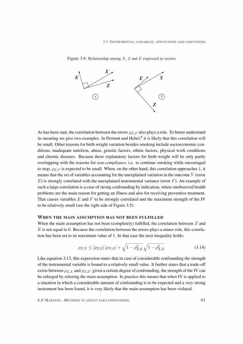
A LIMIT ON THE STRENGTH OF INSTRUMENTS

From the last section it follows that the correlation between a possible instrumental variable andexposure (the strength of the IV ρZ,X ) has to be as strong as possible, which also intuitivelymakes sense. However, in practice it is often difficult to obtain an IV that is strongly relatedto exposure. One reason can be found in the existence of an upper bound on this correlation,which depends on the amount of confounding (indicated by ρX,E), the correlation betweenthe errors in the model (ρE,F ) and the degree of violation of the main assumption (ρZ,E). Wewill further explore the relationship between these correlations, and will distinguish between asituation where the main assumption is fulfilled and one in which it is not.

WHEN THE MAIN ASSUMPTION HAS BEEN FULFILLEDIn case the main assumption of IV has been fulfilled, which means that the IV changes theoutcome only through its relationship with the exposure, it can be shown that

|ρZ,X | =√√√√ 1− ρ2

X,E

ρ2E,F

(3.13)

of which the proof is given in Appendix A. Equation 3.13 indicates that there is a maximum onthe strength of the instrumental variable, and that this maximum decreases when the amountof confounding increases. In case of considerable confounding, the maximum correlationbetween IV and exposure will be quite low. This relationship between the correlations isillustrated in Figure 3.5.

The relation between the strength of the IV ρZ,X and the amount of confounding ρX,E isillustrated by curves representing various levels of the correlation between the errors ρE,F .It can be seen that the maximum correlation between the potential instrumental variableand exposure becomes smaller when the amount of confounding becomes larger. When forexample there is considerable confounding by indication (ρX,E = 0.8), the maximum strengthof the IV is 0.6. Probably this maximum will be even lower because the correlation betweenthe errors will generally be less than 1.0. When for instance ρE,F = 0.85 this maximum dropsto only 0.34.



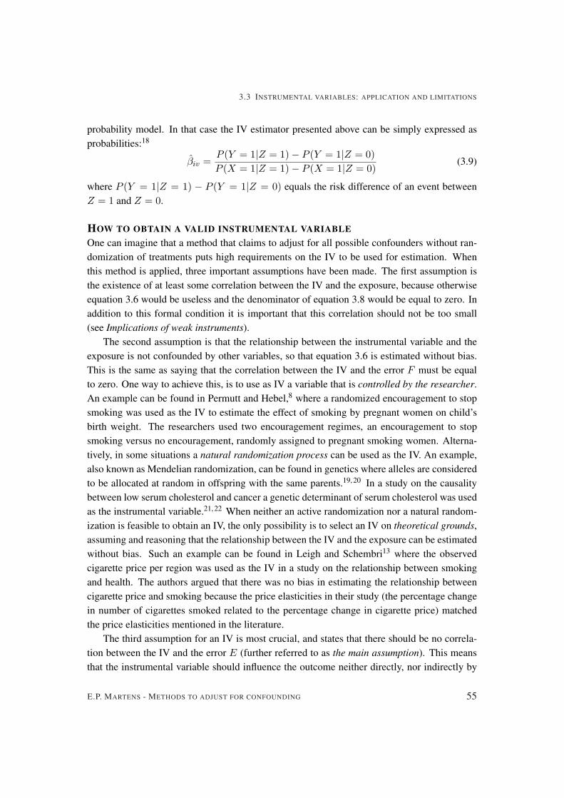
Figure 3.5: Relationship between strength of an instrumental variable (ρZ,X ) and amount of con-founding (ρX,E) for different error correlation levels (ρE,F ), when main assumption has been fulfilled(ρZ,E = 0)

Of the three correlations presented in equation 3.13 and Figure 3.5, the correlation betweenthe errors is most difficult to understand. For the main message, however, its existence is notessential, as is illustrated in Figure 3.6 using vectors.

In panel a of Figure 3.6 the angle between X and E is close to 90◦, meaning that theircorrelation is small (small confounding). Because Z has to be uncorrelated with E accordingto the third IV assumption (perpendicular), the angle between X and Z will be automaticallysmall, indicating a strong IV. In contrast, panel b of Figure 3.6 shows that a large confoundingproblem (small angle between X and E) implies a weak instrument (large angle and smallcorrelation between X and Z). The trade-off between these correlations is an importantcharacteristic of IV estimation. (Note that we simplified the figure by choosing Z in the sameplane as X and Y in order to remove ρE,F from the figure because it equals its maximum of1.0. See Appendix B for the situation in which Z is not in this plane.)



Figure 3.6: Relationship among X , Z and E expressed in vectors

E X

Z

E

X

Z

ba

As has been said, the correlation between the errors ρE,F also plays a role. To better understandits meaning we give two examples. In Permutt and Hebel,8 it is likely that this correlation willbe small. Other reasons for birth weight variation besides smoking include socioeconomic con-ditions, inadequate nutrition, abuse, genetic factors, ethnic factors, physical work conditionsand chronic diseases. Because these explanatory factors for birth weight will be only partlyoverlapping with the reasons for non-compliance, i.e. to continue smoking while encouragedto stop, ρE,F is expected to be small. When, on the other hand, this correlation approaches 1, itmeans that the set of variables accounting for the unexplained variation in the outcome Y (errorE) is strongly correlated with the unexplained instrumental variance (error F ). An example ofsuch a large correlation is a case of strong confounding by indication, where unobserved healthproblems are the main reason for getting an illness and also for receiving preventive treatment.That causes variables E and F to be strongly correlated and the maximum strength of the IVto be relatively small (see the right side of Figure 3.5).

WHEN THE MAIN ASSUMPTION HAS NOT BEEN FULFILLEDWhen the main assumption has not been (completely) fulfilled, the correlation between Z andE is not equal to 0. Because the correlation between the errors plays a minor role, this correla-tion has been set to its maximum value of 1. In that case the next inequality holds:

ρZ,X ≤ |ρZ,E | |ρX,E |+√

1− ρ2Z,E

√1− ρ2

X,E (3.14)

Like equation 3.13, this expression states that in case of considerable confounding the strengthof the instrumental variable is bound to a relatively small value. It further states that a trade-offexists between ρZ,X and ρZ,E : given a certain degree of confounding, the strength of the IV canbe enlarged by relaxing the main assumption. In practice this means that when IV is applied toa situation in which a considerable amount of confounding is to be expected and a very stronginstrument has been found, it is very likely that the main assumption has been violated.



THE EFFECT ON BIASThe limit of the correlation between exposure and instrumental variable has an indirect effecton the bias, because the correlation to be found in practice will be low. This has several dis-advantages that can be illustrated using some previous numerical examples. Suppose we dealwith strong confounding by indication, say ρX,E = 0.80. As has been argued before, this willnaturally imply a strong but imperfect correlation between the errors, say ρE,F = 0.85. In thatcase, the limit of the correlation between exposure and IV will be ρZ,X = 0.34. Restrictingourselves to instrumental variables that fulfill the main assumption (ρZ,E = 0), it will be practi-cally impossible to find an IV that possess the characteristic of being maximally correlated withexposure, which implies that this correlation will be lower than 0.34, for instance 0.20. Withsuch a small correlation, the effect on the bias will be substantial when sample size falls below250 observations. Because we cannot be sure that the main assumption has been fulfilled, caremust be taken even with larger samples sizes.

DISCUSSION

We have focused on the method of instrumental variables for its ability to adjust for confound-ing in non-randomized studies. We have explained the method and its application in a linearmodel and focused on the correlation between the IV and the exposure. When this correlationis very small, this method will lead to an increased standard error of the estimate, a consider-able bias when sample size is small and a bias even in large samples when the main assumptionis only slightly violated. Furthermore, we demonstrated the existence of an upper bound onthe correlation between the IV and the exposure. This upper bound is not a practical limitationwhen confounding is small or moderate because the maximum strength of the IV is still veryhigh. When, on the other hand, considerable confounding by indication exists, the maximumcorrelation between any potential IV and the exposure will be quite low, resulting possibly in afairly weak instrument in order to fulfill the main assumption. Because of a trade-off betweenviolation of this main assumption and the strength of the IV, the presence of considerable con-founding and a strong instrument will probably indicate a violation of the main assumption andthus a biased estimate.

This paper serves as an introduction on the method of instrumental variables demonstratingits merits and limitations. Complexities such as more equations, more instruments, the inclu-sion of covariates and non-linearity of the model have been left out. More equations could beadded with more than two endogenous variables, although it is unlikely to be useful in epidemi-ology when estimating an exposure (treatment) effect. In equation 3.6, multiple instrumentscould be used; this extension does not change the basic ideas behind this method.27 An advan-tage of more than one instrumental variable is that a test on the exogeneity of the instrumentsis possible.16 Another extension is the inclusion of measured covariates in both equations.27

We limited the model to linear regression, assuming that the outcome and the exposure are



both continuous variables, while in medical research dichotomous outcomes or exposures aremore common. The main reason for this choice is simplicity: the application and implicationscan be more easily presented in a linear framework. A dichotomous outcome or dichotomousexposure can easily fit into this model when linearity is assumed using a linear probabilitymodel. Although less known, the results from this model are practically indistinguishable fromlogistic and probit regression analyses, as long as the estimated probabilities range between 0.2and 0.8.28, 29 When risk ratios or log odds are to be analyzed, as in logistic regression analysis,the presented IV-estimator cannot be used and more complex IV-estimators are required. Werefer to the literature for IV-estimation in such cases or in non-linear models in general.6, 30, 31

The limitations when instruments are weak, and the impossibility of finding strong instrumentsin the presence of strong confounding, apply in a similar way.

When assessing the validity of study results, investigators should report both the correlationbetween IV and exposure (or difference in means) and the F-value resulting from equation 3.6and given in equation 3.11. When either of these are small, instrumental variables will not pro-duce unbiased and reasonably precise estimates of exposure effect. Furthermore, it should bemade clear whether the IV is randomized by the researcher, randomized by nature, or is simplyan observed variable. In the latter case, evidence should be given that the various categories ofthe instrumental variable have similar distributions on important characteristics. Additionally,the assumption that the IV determines outcome only by means of exposure is crucial. Becausethis can not be checked, it should be argued theoretically that a direct or indirect relationshipbetween the IV and the outcome is negligible. Finally, in a study in which considerable con-founding can be expected (e.g. strong confounding by indication), one should be aware thatthe existence of a very strong instrument within the IV assumptions is impossible. Whether theinstrument is sufficiently correlated with exposure depends on the number of observations andthe plausibility of the main assumption.

We conclude that the method of IV can be useful in case of moderate confounding, but isless useful when strong confounding (by indication) exists, because strong instruments can notbe found and assumptions will be easily violated.



APPENDIX A

Theorem 1The correlation between Z and X , ρZ,X is bound to obey the equality

|ρZ,X | =√√√√ 1− ρ2

X,E

ρ2E,F

(3.15)

Proof: According to the model one has{

Y = α + βX + E

X = γ + δZ + F

withσZ,E = 0 and σZ,F = 0

It follows from this that σX,E = σγ,E + δ σZ,E + σF,E = 0 + 0 + σE,F = σE,F . Using thisexpression for σX,E one derives that

ρX,E =σX,E

σXσE=

σE,F

σXσE

σF

σF= ρE,F

σF

σX

= ±√

ρ2E,F

σ2F

σ2X

= ±√

ρ2E,F (1− ρ2

Z,X)

Squaring, rearranging terms and taking square roots will give

|ρZ,X | =√√√√1− ρ2

X,E

ρ2E,F

which proves the theorem. ¤



APPENDIX B

The condition ρE,F = 1 is equivalent to the condition that Z is in the same plane as X andE as can be seen in Figure 3.7. For simplicity we assume that the expectation values of thevariables X , Y and Z are all equal to zero.

Figure 3.7: Relationship between X , Z, E and F expressed in vectors

E

F

X

X'

Z

E

X

Z

a b

According to the IV condition that ρZ,E = 0 (these are perpendicular in panel a of Figure 3.7)and the condition that ρZ,F = 0, it follows from panel b of Figure 3.7 that E and F necessarilypoint in the same or opposite direction, implying ρE,F = 1. In this situation there is (up toscalar multiples) only one instrumental variable Z possible in the plane spanned by E and X .As has been argued in the text, it is not likely that this correlation equals 1. This is visualizedin Figure 3.8 where Z is not in the plane spanned by X and E, meaning that F , which is in theplane spanned by X and Z and perpendicular to Z, can impossibly point in the same directionas E. Consequently one then has ρE,F < 1. Here Z ′ is the projection of Z on the planespanned by E and X . The vector Z can now be decomposed as Z = Z ′ + O where Z ′ is inthe plane spanned by E and X and where O is perpendicular to this plane. The vector O canbe referred to as noise because it is uncorrelated to both X and Y . Note that the variable Z ′ isan instrumental variable itself.



Figure 3.8: Three dimensional picture of X , Z, E and noise O expressed in vectors

E

X

Z

Z'

O

V



REFERENCES

[1] Concato J, Shah N, Horwitz RI. Randomized, controlled trials, observational studies, and the hierarchy ofresearch designs. N Engl J Med, 342:1887–1892, 2000.

[2] McMahon AD. Approaches to combat with confounding by indication in observational studies of intendeddrug effects. Pharmacoepidemiol Drug Saf, 12:551–558, 2003.

[3] Klungel OH, Martens EP, Psaty BM, et al. Methods to assess intended effects of drug treatment in observa-tional studies are reviewed. J Clin Epidemiol, 57:1223–1231, 2004.

[4] Rosenbaum PR, Rubin DB. The central role of the propensity score in observational studies for causal effects.Biometrika, 70:41–55, 1983.

[5] Theil H. Principles of Econometrics. Wiley, 1971.

[6] Greenland S. An introduction to instrumental variables for epidemiologists. Int J Epidemiol, 29:722–729,2000.

[7] Zohoori N, Savitz DA. Econometric approaches to epidemiologic data: relating endogeneity and unobservedheterogeneity to confounding. Ann Epidemiol, 7:251–257, 1997. Erratum in: Ann Epidemiol 7:431, 1997.

[8] Permutt Th, Hebel JR. Simultaneous-equation estimation in a clinical trial of the effect of smoking on birthweight. Biometrics, 45:619–622, 1989.

[9] Beck CA, Penrod J, Gyorkos TW, Shapiro S, Pilote L. Does aggressive care following acute myocardialinfarction reduce mortality? Analysis with instrumental variables to compare effectiveness in Canadian andUnited States patient populations. Health Serv Res, 38:1423–1440, 2003.

[10] Brooks JM, Chrischilles EA, Scott SD, Chen-Hardee SS. Was breast conserving surgery underutilized forearly stage breast cancer? Instrumental variables evidence for stage II patients from Iowa. Health Serv Res,38:1385–1402, 2003. Erratum in: Health Serv Res 2004;39(3):693.

[11] Earle CC, Tsai JS, Gelber RD, Weinstein MC, Neumann PJ, Weeks JC. Effectiveness of chemotherapy foradvanced lung cancer in the elderly: instrumental variable and propensity analysis. J Clin Oncol, 19:1064–1070, 2001.

[12] Hadley J, Polsky D, Mandelblatt JS, et al. An exploratory instrumental variable analysis of the outcomes oflocalized breast cancer treatments in a medicare population. Health Econ, 12:171–186, 2003.

[13] Leigh JP, Schembri M. Instrumental variables technique: cigarette price provided better estimate of effectsof smoking on SF-12. J Clin Epidemiol, 57:284–293, 2004.

[14] McClellan M, McNeil BJ, Newhouse JP. Does more intensive treatment of acute myocardial infarction in theelderly reduce mortality? Analysis using instrumental variables. JAMA, 272:859–866, 1994.

[15] McIntosh MW. Instrumental variables when evaluating screening trials: estimating the benefit of detectingcancer by screening. Stat Med, 18:2775–2794, 1999.

[16] Staiger D, Stock JH. Instrumental variables regression with weak instruments. Econometrica, 65:557–586,1997.

[17] Pestman WR. Mathematical Statistics. Walter de Gruyter, Berlin, New York, 1998.

[18] Angrist JD, Imbens GW, Rubin DB. Identification of causal effects using instrumental variables. JASA,91:444–455, 1996.

[19] Thomas DC, Conti DV. Commentary: the concept of ’Mendelian Randomization’. Int J Epidemiol, 33:21–25,2004.

[20] Minelli C, Thompson JR, Tobin MD, Abrams KR. An integrated approach to the meta-analysis of geneticassociation studies using Mendelian Randomization. Am J Epidemiol, 160:445–452, 2004.

[21] Katan MB. Apolipoprotein E isoforms, serum cholesterol, and cancer. Lancet, 1:507–508, 1986.



[22] Smith GD, Ebrahim S. Mendelian randomization: prospects, potentials, and limitations. Int J Epidemiol,33:30–42, 2004.

[23] Bound J, Jaeger DA, Baker RM. Problems with instrumental variables estimation when the correlation be-tween the instruments and the endogenous explanatory variable is weak. JASA, 90:443–450, 1995.

[24] Sawa T. The exact sampling distribution of ordinary least squares and two-stage least squares estimators. JAm Stat Ass, 64:923–937, 1969.

[25] Nelson CR, Startz R. Some further results on the exact small sample properties of the instrumental variableestimator. Econometrica, 58:967–976, 1990.

[26] Angrist JD, Krueger AB. Split sample instrumental variables. J Bus and Econ Stat, 13:225–235, 1995.

[27] Angrist JD, Imbens GW. Two-stage least squares estimation of average causal effects in models with variabletreatment intensity. JASA, 90:431–442, 1995.

[28] Cox DR, Snell EJ. Analysis of Binary Data. Chapman and Hall, 1989.

[29] Cox DR, Wermuth N. A comment on the coefficient of determination for binary responses. The AmericanStatistician, 46:1–4, 1992.

[30] Bowden RJ, Turkington DA. A comparative study of instrumental variables estimators for nonlinear simulta-neous models. J Am Stat Ass, 76:988–995, 1981.

[31] Amemiya T. The nonlinear two-stage least-squares estimator. Journal of econometrics, 2:105–110, 1974.


strengths and limitations of adjustment … · in medical research logistic regression and cox...

Documents