string branes and superstring theory
DESCRIPTION
Modern physicsTRANSCRIPT

arX
iv:h
ep-t
h/01
1005
5 v3
3
Jan
2002 Strings, Branes and
Extra Dimensions
Stefan Forste
Physikalisches Institut, Universitat BonnNussallee 12, D-53115 Bonn, Germany
Abstract
This review is devoted to strings and branes. Firstly, perturbative string theory isintroduced. The appearance of various types of branes is discussed. These include
orbifold fixed planes, D-branes and orientifold planes. The connection to BPS vacuaof supergravity is presented afterwards. As applications, we outline the role of branes
in string dualities, field theory dualities, the AdS/CFT correspondence and scenarioswhere the string scale is at a TeV. Some issues of warped compactifications are also
addressed. These comprise corrections to gravitational interactions as well as thecosmological constant problem.

Contents
1 Introduction 1
2 Perturbative description of branes 42.1 The Fundamental String . . . . . . . . . . . . . . . . . . . . . . . . . . 4
2.1.1 Worldsheet Actions . . . . . . . . . . . . . . . . . . . . . . . . . 42.1.1.1 The closed bosonic string . . . . . . . . . . . . . . . . 4
2.1.1.2 Worldsheet supersymmetry . . . . . . . . . . . . . . . 72.1.1.3 Space-time supersymmetric string . . . . . . . . . . . 10
2.1.2 Quantization of the fundamental string . . . . . . . . . . . . . 132.1.2.1 The closed bosonic string . . . . . . . . . . . . . . . . 14
2.1.2.2 Type II strings . . . . . . . . . . . . . . . . . . . . . . 192.1.2.3 The heterotic string . . . . . . . . . . . . . . . . . . . 25
2.1.3 Strings in non-trivial backgrounds . . . . . . . . . . . . . . . . 28
2.1.4 Perturbative expansion and effective actions . . . . . . . . . . . 362.1.5 Toroidal Compactification and T-duality . . . . . . . . . . . . . 42
2.1.5.1 Kaluza-Klein compactification of a scalar field . . . . 422.1.5.2 The bosonic string on a circle . . . . . . . . . . . . . . 43
2.1.5.3 T-duality in non trivial backgrounds . . . . . . . . . . 462.1.5.4 T-duality for superstrings . . . . . . . . . . . . . . . . 48
2.2 Orbifold fixed planes . . . . . . . . . . . . . . . . . . . . . . . . . . . . 502.2.1 The bosonic string on an orbicircle . . . . . . . . . . . . . . . . 51
2.2.2 Type IIB on T 4/Z2 . . . . . . . . . . . . . . . . . . . . . . . . . 542.2.3 Comparison with type IIB on K3 . . . . . . . . . . . . . . . . . 57
2.3 D-branes . . . . . . . . . . . . . . . . . . . . . . . . . . . . . . . . . . . 61
2.3.1 Open strings . . . . . . . . . . . . . . . . . . . . . . . . . . . . 612.3.1.1 Boundary conditions . . . . . . . . . . . . . . . . . . . 61
2.3.1.2 Quantization of the open string ending on a single D-brane . . . . . . . . . . . . . . . . . . . . . . . . . . . 65
2.3.1.3 Number of ND directions and GSO projection . . . . 672.3.1.4 Multiple parallel D-branes – Chan Paton factors . . . 68
2.3.2 D-brane interactions . . . . . . . . . . . . . . . . . . . . . . . . 702.3.3 D-brane actions . . . . . . . . . . . . . . . . . . . . . . . . . . . 78
2.3.3.1 Open strings in non-trivial backgrounds . . . . . . . . 792.3.3.2 Toroidal compactification and T-duality for open strings 852.3.3.3 RR fields . . . . . . . . . . . . . . . . . . . . . . . . . 91
i

CONTENTS ii
2.3.3.4 Noncommutative geometry . . . . . . . . . . . . . . . 932.4 Orientifold fixed planes . . . . . . . . . . . . . . . . . . . . . . . . . . 98
2.4.1 Unoriented closed strings . . . . . . . . . . . . . . . . . . . . . 982.4.2 O-plane interactions . . . . . . . . . . . . . . . . . . . . . . . . 101
2.4.2.1 O-plane/O-plane interaction, or the Klein bottle . . . 1012.4.2.2 D-brane/O-plane interaction, or the Mobius strip . . 107
2.4.3 Compactifying the transverse dimensions . . . . . . . . . . . . 1122.4.3.1 Type I/type I′ strings . . . . . . . . . . . . . . . . . . 113
2.4.3.2 Orbifold compactification . . . . . . . . . . . . . . . . 116
3 Non-Perturbative description of branes 1243.1 Preliminaries . . . . . . . . . . . . . . . . . . . . . . . . . . . . . . . . 1243.2 Universal Branes . . . . . . . . . . . . . . . . . . . . . . . . . . . . . . 125
3.2.1 The fundamental string . . . . . . . . . . . . . . . . . . . . . . 1273.2.2 The NS five brane . . . . . . . . . . . . . . . . . . . . . . . . . 131
3.3 Type II branes . . . . . . . . . . . . . . . . . . . . . . . . . . . . . . . 134
4 Applications 1384.1 String dualities . . . . . . . . . . . . . . . . . . . . . . . . . . . . . . . 138
4.2 Dualities in Field Theory . . . . . . . . . . . . . . . . . . . . . . . . . 1414.3 AdS/CFT correspondence . . . . . . . . . . . . . . . . . . . . . . . . . 145
4.3.1 The conjecture . . . . . . . . . . . . . . . . . . . . . . . . . . . 1464.3.2 Wilson loop computation . . . . . . . . . . . . . . . . . . . . . 149
4.3.2.1 Classical approximation . . . . . . . . . . . . . . . . . 149
4.3.2.2 Stringy corrections . . . . . . . . . . . . . . . . . . . . 1544.4 Strings at a TeV . . . . . . . . . . . . . . . . . . . . . . . . . . . . . . 161
4.4.1 Corrections to Newton’s law . . . . . . . . . . . . . . . . . . . . 165
5 Brane world setups 1675.1 The Randall Sundrum models . . . . . . . . . . . . . . . . . . . . . . . 167
5.1.1 The RS1 model with two branes . . . . . . . . . . . . . . . . . 1675.1.1.1 A proposal for radion stabilization . . . . . . . . . . . 171
5.1.2 The RS2 model with one brane . . . . . . . . . . . . . . . . . . 1745.1.2.1 Corrections to Newton’s law . . . . . . . . . . . . . . 1755.1.2.2 ... and the holographic principle . . . . . . . . . . . . 179
5.1.2.3 The RS2 model with two branes . . . . . . . . . . . . 1815.2 Inclusion of a bulk scalar . . . . . . . . . . . . . . . . . . . . . . . . . 183
5.2.1 A solution generating technique . . . . . . . . . . . . . . . . . . 1835.2.2 Consistency conditions . . . . . . . . . . . . . . . . . . . . . . . 186
5.2.3 The cosmological constant problem . . . . . . . . . . . . . . . . 1885.2.3.1 An example . . . . . . . . . . . . . . . . . . . . . . . . 189
5.2.3.2 A no go theorem . . . . . . . . . . . . . . . . . . . . . 193

CONTENTS iii
6 Bibliography and further reading 1976.1 Chapter 2 . . . . . . . . . . . . . . . . . . . . . . . . . . . . . . . . . . 197
6.1.1 Books . . . . . . . . . . . . . . . . . . . . . . . . . . . . . . . . 1976.1.2 Review articles . . . . . . . . . . . . . . . . . . . . . . . . . . . 198
6.1.3 Research papers . . . . . . . . . . . . . . . . . . . . . . . . . . 1986.2 Chapter 3 . . . . . . . . . . . . . . . . . . . . . . . . . . . . . . . . . . 200
6.2.1 Review articles . . . . . . . . . . . . . . . . . . . . . . . . . . . 2006.2.2 Research Papers . . . . . . . . . . . . . . . . . . . . . . . . . . 200
6.3 Chapter 4 . . . . . . . . . . . . . . . . . . . . . . . . . . . . . . . . . . 2006.3.1 Review articles . . . . . . . . . . . . . . . . . . . . . . . . . . . 200
6.3.2 Research papers . . . . . . . . . . . . . . . . . . . . . . . . . . 2016.4 Chapter 5 . . . . . . . . . . . . . . . . . . . . . . . . . . . . . . . . . . 202
6.4.1 Review articles . . . . . . . . . . . . . . . . . . . . . . . . . . . 202
6.4.2 Research papers . . . . . . . . . . . . . . . . . . . . . . . . . . 202

Chapter 1
Introduction
One of the most outstanding problems of theoretical physics is to unify our picture of
electroweak and strong interactions with gravitational interactions. We would like to
view the attraction of masses as appearing due to the exchange of particles (gravitons)
between the masses. In conventional perturbative quantum field theory this is not
possible because the theory of gravity is not renormalizable. A promising candidate
providing a unified picture is string theory. In string theory, gravitons appear together
with the other particles as excitations of a string.
On the other hand, also from an observational point of view gravitational interac-
tions show some essential differences to the other interactions . Masses always attract
each other, and the strength of the gravitational interaction is much weaker than the
electroweak and strong interactions. A way how this difference could enter a theory
is provided by the concept of “branes”. The expression “brane” is derived from mem-
brane and stands for extended objects on which interactions are localized. Assuming
that gravity is the only interaction which is not localized on a brane, the special fea-
tures of gravity can be attributed to properties of the extra dimensions where only
gravity can propagate. (This can be either the size of the extra dimension or some
curvature.)
The brane picture is embedded in a natural way in string theory. Therefore, string
theory has the prospect to unify gravity with the strong and electroweak interactions
while, at the same time, explaining the difference between gravitational and the other
interactions.
This set of notes is organized as follows. In chapter 2, we briefly introduce the
concept of strings and show that quantized closed strings yield the graviton as a string
excitation. We argue that the quantized string lives in a ten dimensional target space.
It is shown that an effective field theory description of strings is given by (higher di-
mensional supersymmetric extensions of) the Einstein Hilbert theory. The concept
1
1. Introduction 2
of compactifying extra dimensions is introduced and special stringy features are em-
phasized. Thereafter, we introduce the orbifold fixed planes as higher dimensional
extended objects where closed string twisted sector excitations are localized. The
quantization of the open string will lead us to the concept of D-branes, branes on
which open string excitations live. We compute the tensions and charges of D-branes
and derive an effective field theory on the world volume of the D-brane. Finally,
perturbative string theory contains orientifold planes as extended objects. These are
branes on which excitations of unoriented closed strings can live. Compactifications
containing orientifold planes and D-branes are candidates for phenomenologically in-
teresting models. We demonstrate the techniques of orientifold compactifications at a
simple example.
In chapter 3, we identify some of the extended objects of chapter 2 as stable
solutions of the effective field theory descriptions of string theory. These will be the
fundamental string and the D-branes. In addition we will find another extended object,
the NS five brane, which cannot be described in perturbative string theory.
Chapter 4 discusses some applications of the properties of branes derived in the
previous chapters. One of the problems of perturbative string theory is that the string
concept does not lead to a unique theory. However, it has been conjectured that all
the consistent string theories are perturbative descriptions of one underlying theory
called M-theory. We discuss how branes fit into this picture. We also present branes
as tools for illustrating duality relations among field theories. Another application, we
are discussing is based on the twofold description of three dimensional D-branes. The
perturbative description leads to an effective conformal field theory (CFT) whereas the
corresponding stable solution to supergravity contains an AdS space geometry. This
observation results in the AdS/CFT correspondence. We present in some detail, how
the AdS/CFT correspondence can be employed to compute Wilson loops in strongly
coupled gauge theories. An application which is of phenomenological interest is the
fact that D-branes allow to construct models in which the string scale is of the order of
a TeV. If such models are realized in nature, they should be discovered experimentally
in the near future.
Chapter 5 is somewhat disconnected from the rest of these notes since it considers
brane models which are not directly constructed from strings. Postulating the existence
of branes on which certain interactions are localized, we present the construction of
models in which the space transverse to the brane is curved. We discuss how an
observer on a brane experiences gravitational interactions. We also make contact to the
AdS/CFT conjecture for a certain model. Also other questions of phenomenological
relevance are addressed. These are the hierarchy problem and the problem of the
cosmological constant. We show how these problems are modified in models containing

1. Introduction 3
branes.
Chapter 6 gives hints for further reading and provides the sources for the current
text.
Our intention is that this review should be self contained and be readable by people
who know some quantum field theory and general relativity. We hope that some people
will enjoy reading one or the other section.

Chapter 2
Perturbative description of
branes
2.1 The Fundamental String
2.1.1 Worldsheet Actions
2.1.1.1 The closed bosonic string
Let us start with the simplest string – the bosonic string. The string moves along a
surface through space and time. This surface is called the worldsheet (in analogy to a
worldline of a point particle). For space and time in which the motion takes place we
will often use the term target space. Let d be the number of target space dimesnions.
The coordinates of the target space are Xµ, and the worldsheet is a surface Xµ (τ, σ),
where τ and σ are the time and space like variables parameterizing the worldsheet.
String theory is defined by the requirement that the classical motion of the string
should be such that its worldsheet has minimal area. Hence, we choose the action of
the string proportional to the worldsheet. The resulting action is called Nambu Goto
action. It reads
S = − 1
2πα′
∫d2σ√−g. (2.1.1.1)
The integral is taken over the parameter space of σ and τ . (We will also use the
notation τ = σ0, and σ = σ1.) The determinant of the induced metric is called g. The
induced metric depends on the shape of the worldsheet and the shape of the target
space,
gαβ = Gµν (X)∂αXµ∂βX
ν , (2.1.1.2)
4
2. Worldsheet Actions 5
where µ, ν label target space coordinates, whereas α, β label worldsheet parameters.
Finally, we have introduced a constant α′. It is the inverse of the string tension and
has the mass dimension −2. The choice of this constant sets the string scale. By con-
struction, the action (2.1.1.1) is invariant under reparametrizations of the worldsheet.
Alternatively, we could have introduced an independent metric γαβ on the world-
sheet. This enables us to write the action (2.1.1.1) in an equivalent form,
S = − 1
4πα′
∫d2σ√−γγαβGµν∂αXµ∂βX
ν . (2.1.1.3)
For the target space metric we will mostly use the Minkowski metric ηµν in the present
chapter. Varying (2.1.1.3) with respect to γαβ yields the energy momentum tensor,
Tαβ = − 4πα′√−γδS
δγαβ= ∂αX
µ∂βXµ −1
2γαβγ
δγ∂δXµ∂γXµ, (2.1.1.4)
where the target space index µ is raised and lowered with Gµν = ηµν . Thus, the γαβ
equation of motion, Tαβ = 0, equates γαβ with the induced metric (2.1.1.2), and the
actions (2.1.1.1) and (2.1.1.3) are at least classically equivalent. If we had just used
covariance as a guiding principle we would have written down a more general expression
for (2.1.1.3). We will do so later. At the moment, (2.1.1.3) with Gµν = ηµν describes
a string propagating in the trivial background. Upon quantization of this theory we
will see that the string produces a spectrum of target space fields. Switching on non
trivial vacua for those target space fields will modify (2.1.1.3). But before quantizing
the theory, we would like to discuss the symmetries and introduce supersymmetric
versions of (2.1.1.3).
First of all, (2.1.1.3) respects the target space symmetries encoded in Gµν . In
our case Gµν = ηµν this is nothing but d dimensional Poincare invariance. From
the two dimensional point of view, this symmetry corresponds to field redefinitions
in (2.1.1.3). The action is also invariant under two dimensional coordinate changes
(reparametrizations). Further, it is Weyl invariant, i.e. it does not change under
γαβ → eϕ(τ,σ)γαβ. (2.1.1.5)
It is this property which makes one dimensional objects special. The two dimensional
coordinate transformations together with the Weyl transformations are sufficient to
transform the worldsheet metric locally to the Minkowski metric,
γαβ = ηαβ. (2.1.1.6)
It will prove useful to use instead of σ0, σ1 the light cone coordinates,
σ− = τ − σ , and σ+ = τ + σ. (2.1.1.7)

2. Worldsheet Actions 6
So, the gauged fixed version1 of (2.1.1.3) is
S =1
2πα′
∫dσ+dσ−∂−X
µ∂+Xµ. (2.1.1.8)
However, the reparametrization invariance is not completely fixed. There is a residual
invariance under the conformal coordinate transformations,
σ+ → σ+(σ+)
, σ− → σ−(σ−). (2.1.1.9)
This invariance is connected to the fact that the trace of the energy momentum tensor
(2.1.1.4) vanishes identically, T+− = 02 . However, the other γαβ equations are not
identically satisfied and provide constraints, supplementing (2.1.1.8),
T++ = T−− = 0. (2.1.1.10)
The equations of motion corresponding to (2.1.1.8) are3
∂+∂−Xµ = 0 (2.1.1.11)
Employing conformal invariance (2.1.1.9) we can choose τ to be an arbitrary solution
to the equation ∂+∂−τ = 0. (The combination of (2.1.1.9) and (2.1.1.7) gives
τ → 1
2
(σ+(σ+)
+ σ−(σ−)), (2.1.1.12)
which is the general solution to (2.1.1.11)). Hence, without loss of generality we can
fix
X+ =1√2
(X0 + X1
)= x+ + p+τ, (2.1.1.13)
where x+ and p+ denote the center of mass position and momentum of the string in
the + direction, respectively. The constraint equations (2.1.1.10) can now be used to
fix
X− =1√2
(X0 −X1
)(2.1.1.14)
as a function of X i (i = 2, . . . , d − 1) uniquely up to an integration constant corre-
sponding to the center of mass position in the minus direction. Thus we are left with
1Gauge fixing means imposing (2.1.1.6).2The corresponding symmetry is called conformal symmetry. It means that the action is invari-
ant under conformal coordinate transformations while keeping the worldsheet metric fixed. In twodimensions this is equivalent to Weyl invariance.
3For the time being we will focus on closed strings. That means that we impose periodic boundaryconditions and hence there are no boundary terms when varying the action. We will discuss openstrings when turning to the perturbative description of D-branes in section 2.3.

2. Worldsheet Actions 7
d−2 physical degrees of freedom X i. Their equations of motion are (2.1.1.11) without
any further constraints. By employing the symmetries of (2.1.1.3) we managed to
reduce the system to d − 2 free fields (satisfying (2.1.1.11)). Since these symmetries
may suffer from quantum anomalies we will have to be careful when quantizing the
theory in section 2.1.2.
2.1.1.2 Worldsheet supersymmetry
In this section we are going to modify the previously discussed bosonic string by
enhancing its two dimensional symmetries. We will start from the gauge fixed ac-
tion (2.1.1.8) which had as residual symmetries two dimensional Poincare invariance
and conformal coordinate transformations (2.1.1.9).4 A natural extension of Poincare
invariance is supersymmetry. Therefore, we will study theories which are supersym-
metric from the two dimensional point of view. In order to construct a supersymmet-
ric extension of (2.1.1.8) one should first specify the symmetry group and then use
Noether’s method to build an invariant action. We will be brief and just present the
result,
S =1
2πα′
∫dσ+dσ−
(∂−X
µ∂+Xµ +i
2ψµ+∂−ψ+µ +
i
2ψµ−∂+ψ−µ
), (2.1.1.15)
where ψ± are two dimensional Majorana-Weyl spinors. To see this, we first note that
iψ+∂−ψ+ + iψ−∂+ψ− = −1
2(ψ+,−ψ−)
(ρ+∂+ + ρ−∂−
)(ψ−ψ+
), (2.1.1.16)
where
ρ± = ρ0 ± ρ1, (2.1.1.17)
with
ρ0 =
(0 −ii 0
)and ρ1 =
(0 i
i 0
). (2.1.1.18)
It is easy to check that the above matrices form a two dimensional Clifford algebra,ρα, ρβ
= −2ηαβ. (2.1.1.19)
Also, note that i (ψ+,−ψ−) is the Dirac conjugate of
(ψ−ψ+
)for real ψ±, i.e. of the
Majorana spinor
(ψ−ψ+
). In addition to two dimensional Poincare invariance and
4Alternatively, we could start from the action (2.1.1.3). This we would modify such that it becomeslocally supersymmetric. Finally, we would fix symmetries in the locally supersymmetric action.

2. Worldsheet Actions 8
invariance under conformal coordinate transformations (2.1.1.9)5 the action (2.1.1.15)
is invariant under worldsheet supersymmetry,
δXµ = εψµ = iε+ψµ− − iε−ψµ+, (2.1.1.20)
δψµ = −iρα∂αXµε. (2.1.1.21)
In components (2.1.1.21) gives rise to the two equations
δψµ− = −2ε+∂−Xµ, (2.1.1.22)
δψµ+ = 2ε−∂+Xµ. (2.1.1.23)
When checking the invariance of (2.1.1.15) under (2.1.1.20), (2.1.1.22), (2.1.1.23) one
should take into account that spinor components are anticommuting, e.g. ε+ψ− =
−ψ−ε+. Since the supersymmetry parameters ε± form a non chiral Majorana spinor,
the above symmetry is called (1, 1) supersymmetry. (In the end of this section we will
also discuss the chiral (1, 0) supersymmetry.) To summarize, the action (2.1.1.15) has
the following two dimensional global symmetries: Poincare invariance and supersym-
metry. The corresponding Noether currents are the energy momentum tensor,
T++ = ∂+Xµ∂+Xµ +
i
2ψµ+∂+ψ+µ, (2.1.1.24)
T−− = ∂−Xµ∂−Xµ +i
2ψµ−∂−ψ−µ, (2.1.1.25)
and the supercurrent
J+ = ψµ+∂+Xµ, (2.1.1.26)
J− = ψµ−∂−Xµ. (2.1.1.27)
The vanishing of the trace of the energy momentum tensor T+− ≡ 0 is again a con-
sequence of the invariance under the (local) conformal coordinate transformations
(2.1.1.9). The supercurrent is a spin–32 object and naively one would expect to get
four independent components. That there are only two non-vanishing components is
a consequence of the fact that the supersymmetries (2.1.1.20), (2.1.1.22), (2.1.1.23)
leave the action invariant also when we allow instead of constant ε± for
ε− = ε−(σ+)
and ε+ = ε+(σ−), (2.1.1.28)
i.e. they are “partially” local symmetries. Once again, the vanishing of the energy
momentum tensor is an additional constraint on the system. We did not derive this
5Under the transformation (2.1.1.9) the spinor components transform as ψ± →(σ±′)− 1
2 ψ± .

2. Worldsheet Actions 9
explicitly here. But it can be easily inferred as follows. In two dimensions the Einstein
tensor vanishes identically. Thus, if we were to couple to two dimensional (Einstein)
gravity, the constraint Tαβ = 0 would correspond to the Einstein equation. Simi-
larly, the supercurrents (2.1.1.26), (2.1.1.27) are constrained to vanish. (If the theory
was coupled to two dimensional supergravity, this would correspond to the gravitino
equations of motion.)
As in the bosonic case we can employ the symmetry (2.1.1.9) to fix
X+ = x+ + p+τ. (2.1.1.29)
The local supersymmetry transformation (2.1.1.21) with ε given by (2.1.1.28) can be
used to gauge
(ψ−ψ+
)µ=+
= 0. (2.1.1.30)
(We have written here the target space (light cone) index as µ = + in order to avoid
confusion with the worldsheet spinor indices.) Note, that the gauge fixing condi-
tion (2.1.1.30) is compatible with (2.1.1.29) and the supersymmetry transformations
(2.1.1.20), (2.1.1.21), as (2.1.1.30) implies the supersymmetry transformation
δX+ = 0. (2.1.1.31)
The constraints (2.1.1.24), (2.1.1.25), (2.1.1.26), (2.1.1.27) can be solved for X−, and
ψµ=−α (here, α denotes the worldsheet spinor index). Therefore, after fixing the local
symmetries completely we are left with d− 2 free bosons and d− 2 free fermions (from
a two dimensional point of view).
We should note that in the closed string case (periodic boundary conditions in
bosonic directions) we have two choices for boundary conditions on the worldsheet
fermions. Boundary terms appearing in the variation of the action vanish for either
periodic or anti periodic boundary conditions on worldsheet fermions. (Later, we will
call the solutions with antiperiodic fermions Neveu Schwarz (NS) sector and the ones
with periodic boundary conditions Ramond (R) sector.
Going back to (2.1.1.15), we note that alternatively we could have written down
a (1, 0) supersymmetric action by setting the left handed fermions ψµ+ = 0. The
supersymmetries are now given by (2.1.1.20) and (2.1.1.22), only. The parameter ε−does not occur anymore, and hence we have reduced the number of supersymmetries by
one half. More generally one can add left handed fermions λA+ which do not transform
under supersymmetries. Therefore, they do not need to be in the same representation
of the target space Lorentz group as the Xµ (therefore the index A instead of µ).

2. Worldsheet Actions 10
Summarizing we obtain the following (1, 0) supersymmetric action
S =1
2πα′
∫dσ+dσ−
(∂−X
µ∂+Xµ +i
2ψµ−∂+ψ−µ +
i
2
N∑
A=1
λA+∂−λ+A
). (2.1.1.32)
this will turn out to be the worldsheet action of the heterotic string. The energy mo-
mentum tensor is as given in (2.1.1.24), (2.1.1.25) with λA+ replacing ψµ+ in (2.1.1.25).
There is only one conserved supercurrent (2.1.1.26).
Finally, we should remark that there are also extended versions of two dimensional
supersymmetry (see for example [456]). We will not be dealing with those in this
review.
2.1.1.3 Space-time supersymmetric string
In the above we have extended the bosonic string (2.1.1.3) to a superstring from the two
dimensional perspective. We called this worldsheet supersymmetry. Another direction
would be to extend (2.1.1.3) such that the target space Poincare invariance is enhanced
to target space supersymmetry. This concept leads to the Green Schwarz string. Space
time supersymmetry means that the bosonic coordinates Xµ get fermionic partners θA
(where A labels the number of supersymmetries N) such that the targetspace becomes
a superspace. In addition to Lorentz symmetry, the supersymmetric extension mixes
fermionic and bosonic coordinates,
δθA = εA, (2.1.1.33)
δθ = εA, (2.1.1.34)
δXµ = iεΓµθA, (2.1.1.35)
where the global transformation parameter εA is a target space spinor and Γµ denotes
a target space Dirac matrix. In order to construct a string action respecting the
symmetries (2.1.1.33) – (2.1.1.35) one tries to replace ∂αXµ by the supersymmetric
combination
Πµα = ∂αX
µ − iθAΓµ∂αθA . (2.1.1.36)
This leads to the following proposal for a space time supersymmetric string action
S1 = − 1
4πα′
∫d2σ√−γγαβΠµ
αΠβµ. (2.1.1.37)
Note that in contrast to the previously discussed worldsheet supersymmetric string,
(2.1.1.37) consists only of bosons when looked at from a two dimensional point of view.
The action (2.1.1.37) is invariant under global target space supersymmetry, i.e. Lorentz

2. Worldsheet Actions 11
transformations plus the supersymmetry transformations (2.1.1.33) – (2.1.1.35). From
the worldsheet perspective we have reparametrization invariance and Weyl invariance
(2.1.1.5). This is again enough to fix the worldsheet metric γαβ = ηαβ (cf (2.1.1.6)).
The resulting action will exhibit conformal coordinate transformations (2.1.1.9) as
residual symmetries. The energy momentum tensor ((2.1.1.4) with ∂αXµ replaced by
Πµα (2.1.1.36)) is again traceless. Like in section 2.1.1.1, the vanishing of the energy mo-
mentum tensor gives two constraints. We have seen that in the non-supersymmetric
case fixing conformal coordinate transformations and solving the constraints leaves
effectively d− 2 (transversal) bosonic directions.6 In order for the target space super-
symmetry not to be spoiled in this process, we would like to reduce the number of
fermionic directions θA by a factor of
2[d−2]
2
2[d]2
=1
2
simultaneously. So, we need an additional local symmetry whose gauge fixing will
remove half of the fermions θA. The symmetry we are looking for is known as κ
symmetry. It exists only in special circumstances. First of all, the number of super-
symmetries should not exceed N = 2 (i.e. A = 1, 2). Then, adding a further term
S2 =1
2πα′
∫d2σ
−iεαβ∂αXµ
(θ1Γµ∂βθ
1 − θ2Γµ∂βθ2)
+εαβ θ1Γµ∂αθ1θ2Γµ∂βθ
2
(2.1.1.38)
to (2.1.1.37) results in a κ symmetric action. (We will give the explicit transformations
below.) In (2.1.1.38) εαβ denotes the two dimensional Levi Civita symbol. If one is
interested in less than N = 2 one can just put the corresponding θA to zero. The
requirement that adding S2 to the action does not spoil supersymmetry (2.1.1.33) –
(2.1.1.35), leads to further constraints,
(i) d = 3 and θ is Majorana
(ii) d = 4 and θ is Majorana or Weyl
(iii) d = 6 and θ is Weyl
(iv) d = 10 and θ is Majorana-Weyl.It remains to give the above mentioned κ symmetry transformations explicitly.
By adding S1 and S2 one observes that the kinetic terms for the θ’s (terms with one
derivative acting on a fermion) contain the following projection operators
Pαβ± =1
2
(γαβ ± εαβ√−γ
). (2.1.1.39)
6Since the field equations are different for (2.1.1.37) the details of the discussion in the bosonic casewill change. The above frame just gives a rough motivation for a modification of (2.1.1.37) carriedout below.
2. Worldsheet Actions 12
The transformation parameter for the additional local symmetry is called κAα . It is a
spinor from the target space perspective and in addition a worldsheet vector subject
to the following constraints
κ1α = Pαβ− κ1β , (2.1.1.40)
κ2α = Pαβ+ κ2
β , (2.1.1.41)
(2.1.1.42)
where the worldsheet indices α, β are raised and lowered with respect to the worldsheet
metric γαβ. Now, we are ready to write down the κ transformations,
δθA = 2iΓµΠαµκAα, (2.1.1.43)
δXµ = iθAΓµδθA, (2.1.1.44)
δ(√−γγαβ
)= −16
√−γ(Pαγ− κ1β∂γθ
1 + Pαγ+ κ2β∂γθ
2). (2.1.1.45)
For a proof that these transformations leave S1 + S2 indeed invariant we refer to[222]
for example.
Once we have established that the number of local symmetries is correct, we can
now proceed to employ those symmetries and reduce the number of degrees of freedom
by gauge fixing. We will go to the light cone gauge in the following. Here, we will
discuss only the most interesting case of d = 10. As usual we use reparametrization
and Weyl invariance to fix γαβ = ηαβ. We can fix κ symmetry (2.1.1.43)–(2.1.1.45) by
the choice
Γ+θ1 = Γ+θ2 = 0, (2.1.1.46)
where
Γ± =1√2
(Γ0 ± Γ9
). (2.1.1.47)
This sets half of the components of θ to zero. With the κ fixing condition (2.1.1.46)
the equations of motion for X+ and X i (i = 2, . . . , d − 1) turn out to be free field
equations (cf (2.1.1.11)). The reason for this can be easily seen as follows. After
imposing (2.1.1.46), out of the fermionic terms only those containing θAΓ−θA remain
in the action S1 + S2. Especially, the terms fourth order in θA have gone. The above
mentioned terms with Γ− couple to ∂αX+, and hence they will only have influence
on the X− equation (obtained by taking the variation of the action with respect to
X+). Thus we can again fix the conformal coordinate transformations by the choice
(2.1.1.13). TheX− direction is then fixed (up to a constant) by imposing the constraint
of vanishing energy momentum tensor. Since the coupling of bosons and fermions is
2. Quantization of the fundamental string 13
reduced to a coupling to ∂αX+, there is just a constant p+ in front of the free kinetic
terms of the fermions.
In the light-cone gauge described above the target space symmetry has been fixed
up to the subgroup SO(8), where the X i and the θA transform in eight dimensional
representations.7 For SO(8) there are three inequivalent eight dimensional representa-
tions, called 8v, 8s , and 8c. The group indices are chosen as i, j, k for the 8v, a, b, c for
the 8s, and a, b, c for the 8c. In particular, X i transforms in the vector representation
8v. For the target space spinors we can choose either 8s or 8c. Absorbing also the
constant in front of the kinetic terms in a field redefinition we specify this choice by
the following notation
√p+θ1 → S1a or S1a (2.1.1.48)
√p+θ2 → S2a or S2a. (2.1.1.49)
Essentially, we have here two different cases: we take the same SO(8) representation
for both θ’s or we take them mutually different. The first option results in type IIB
theory whereas the second one leads to type IIA.
So, the gauge fixing procedure simplifies the theory substantially. The equations of
motion for the remaining degrees of freedom are just free field equations. For example
for the type IIB theory they read,
∂+∂−Xi = 0, (2.1.1.50)
∂+S1a = 0, (2.1.1.51)
∂−S2a = 0. (2.1.1.52)
They look almost equivalent to the equations of motion one obtains from the world-
sheet supersymmetric action (2.1.1.15) after eliminating the ± directions by the light
cone gauge. Especially, (2.1.1.51) and (2.1.1.52) have the form of two dimensional
Dirac equations where S1 and S2 appear as 2d Majorana-Weyl spinors. An important
difference is however, that in (2.1.1.15) all worldsheet fields transform in the vector
representation of the target space subgroup SO(d− 2).
In the rest of this chapter we will focus only on the worldsheet supersymmetric
formulation. There, target space fermions will appear in the Hilbert space when quan-
tizing the theory. We will come back to the Green Schwarz string only when discussing
type IIB strings living in a non-trivial target space (AdS5 × S5) in section 4.3.
2.1.2 Quantization of the fundamental string
7A Majorana-Weyl spinor in ten dimensions has 16 real components. Imposing (2.1.1.46) leaveseight.

2. Quantization of the fundamental string 14
2.1.2.1 The closed bosonic string
Our starting point is equation (2.1.1.11).
∂+∂−Xi = 0. (2.1.2.1)
Imposing periodicity under shifts of σ1 by π we obtain the following general solutions8
Xµ = XµR
(σ−)
+ XµL
(σ+), (2.1.2.2)
with
XµR =
1
2xµ +
1
2pµσ− +
i
2
∑
n6=0
1
nαµne
−2inσ− , (2.1.2.3)
XµL =
1
2xµ +
1
2pµσ+ +
i
2
∑
n6=0
1
nαµne
−2inσ+. (2.1.2.4)
Here, all σα dependence is written out explicitly, i.e. xµ, pµ, αµn, and αµn are σα
independent operators. Classically, one can associate xµ with the center of mass
position, pµ with the center of mass momentum and αµn (αµn) with the amplitude
of the n’th right moving (left moving) vibration mode of the string in xµ direction.
Reality of Xµ imposes the relations
ᵆn = αµ−n and ᵆn = αµ−n. (2.1.2.5)
We also define a zeroth vibration coefficient via
αµ0 = α
µ0 =
1
2pµ. (2.1.2.6)
Since the canonical momentum is obtained by varying the action (2.1.1.8) with
respect to Xµ (where the dot means derivative with respect to τ) we obtain the
following canonical quantization prescription. The equal time commutators are given
by
[Xµ (σ) , Xν
(σ′)]
=[Xµ (σ) , Xν
(σ′)]
= 0, (2.1.2.7)
and[Xµ (σ) , Xν
(σ′)]
= −iπδ(σ − σ′
)ηµν (2.1.2.8)
where the delta function is a distribution on periodic functions. Formally it can be
assigned a Fourier series
δ (σ) =1
π
∞∑
k=−∞e2ikσ. (2.1.2.9)
8Frequently, we will put α′ = 12. Since it is the only dimensionfull parameter (in the system with
~ = c = 1), it is easy to reinstall it when needed.
2. Quantization of the fundamental string 15
With this we can translate the canonical commutators (2.1.2.7) and (2.1.2.8) into
commutators of the Fourier coefficients appearing in (2.1.2.3) and (2.1.2.4),
[pµ, xν ] = −iηµν , (2.1.2.10)
[αµn, ανk] = nδn+kη
µν , (2.1.2.11)
[αµn, ανk] = nδn+kη
µν , (2.1.2.12)
where δn+k is shorthand for δn+k,0. So far, we did not take into account the constraints
of vanishing energy momentum tensor (2.1.1.10). To do so we go again to the light
cone gauge (2.1.1.13), i.e. set
α+n = α+
n = 0 for n 6= 0. (2.1.2.13)
Now the constraint (2.1.1.10) can be used to eliminate X− (up to x−), or alternatively
the α−n and α−n ,
p+α−n =
∞∑
m=−∞: αin−mα
im : −2aδn, (2.1.2.14)
p+α−n =
∞∑
m=−∞: αin−mα
im : −2aδn (2.1.2.15)
where a sum over repeated indices i from 2 to d− 1 is understood. The colon denotes
normal ordering to be specified below. We have parameterized the ordering ambiguity
by a constant a. (In principle one could have introduced two constants a, a. But this
would lead to inconsistencies which we will not discuss here.) Equations (2.1.2.14) and
(2.1.2.15) are not to be read as operator identities but rather as conditions on physical
states which we will construct now. We choose the vacuum as an eigenstate of the pµ
pµ |k〉 = kµ |k〉 , (2.1.2.16)
with kµ being an ordinary number. Further, we impose that the vacuum is annihilated
by half of the vibration modes,
αin |k〉 = αin |k〉 = 0 for n > 0. (2.1.2.17)
The rest of the states can now be constructed by acting with a certain number of
αi−n and αi−n (n > 0) on the vacuum. But we still need to impose the constraint
(2.1.1.10). Coming back to (2.1.2.14) and (2.1.2.15) we can now specify what is meant
by the normal ordering. The αik (αik) with the greater Fourier index k is written to
the right9. For n 6= 0 (2.1.2.14) and (2.1.2.15) just tell us how any α−n or α−n can be9E.g. for k > 0 this implies that : αikα
i−k := αi−kα
ik, i.e. the annihilation operator acts first on a
state.

2. Quantization of the fundamental string 16
expressed in terms of the αik and αil . The nontrivial information is contained in the
n = 0 case. It is convenient to rewrite (2.1.2.14) and (2.1.2.15) for n = 0,
2p+p− − pipi = 8(N − a) = 8(N − a), (2.1.2.18)
where (doing the normal ordering explicitly)
N =
∞∑
n=1
αi−nαin, (2.1.2.19)
N =
∞∑
n=1
αi−nαin. (2.1.2.20)
The N (N) are number operators in the sense that they count the number of creation
operators αi−n (αi−n) acting on the vacuum. To be precise, the N (N) eigenvalue of
a state is this number multiplied by the index n and summed over all different kinds
of creation operators acting on the vacuum (for left and right movers separately).
Interpreting the pµ eigenvalue kµ as the momentum of a particle (2.1.2.18) looks like
a mass shell condition with the mass squared M2 given by
M2 = 8(N − a) = 8(N − a). (2.1.2.21)
The second equality in the above equation relates the allowed right moving creation
operators acting on the vacuum to the left moving ones. It is known as the level
matching condition.
For example, the first excited state is
αi−1αj−1 |k〉 . (2.1.2.22)
By symmetrizing or antisymmetrizing with respect to i, j and splitting the symmetric
expression into a trace part and a traceless part one sees easily that the states (2.1.2.22)
form three irreducible representations of SO(d − 2). Since we have given the states
the interpretation of being particles living in the targetspace, these should correspond
to irreducible representations of the little group. Only when the above states are
massless the little group is SO(d − 2) (otherwise it is SO(d − 1)). Therefore, for
unbroken covariance with respect to the targetspace Lorentz transformation, the states
(2.1.2.22) must be massless. Comparing with (2.1.2.21) we deduce that the normal
ordering constant a must be one,
a!
= 1. (2.1.2.23)
In the following we are going to compute the normal ordering constant a. Requiring
agreement with (2.1.2.23) will give a condition on the dimension of the targetspace

2. Quantization of the fundamental string 17
to be 26. The following calculation may look at some points a bit dodgy when it
comes to computing the exact value of a. So, before starting we should note that the
compelling result will be that a depends on the targetspace dimension. The exact
numerics can be verified by other methods which we will not elaborate on here for
the sake of briefness. We will consider only N since the calculation with N is a very
straightforward modification (just put tildes everywhere). The initial assumption is
that naturally the ordering in quantum expressions would be symmetric, i.e.
N − a =1
2
∞∑
n=−∞,n6=0
αi−nαin. (2.1.2.24)
By comparison with the definition of N (2.1.2.19) and using the commutation relations
(2.1.2.11) we find
a = −d− 2
2
∞∑
n=1
n. (2.1.2.25)
This expression needs to be regularized. A familiar method of assigning a finite num-
ber to the rhs of (2.1.2.25) is known as ‘zeta function regularization’. One possible
representation of the zeta function is
ζ (s) =
∞∑
n=1
n−s. (2.1.2.26)
The above representation is valid for the real part of s being greater than one. The
zeta function, however, can be defined also for complex s with negative real part. This
is done by analytic continuation. The way to make sense out of (2.1.2.25) is now to
replace the infinite sum by the zeta function
a = −d − 2
2ζ (−1) =
d− 2
24. (2.1.2.27)
Comparing with (2.1.2.23) we see that we need to take
d = 26 (2.1.2.28)
in order to preserve Lorentz invariance. This result can also be verified in a more rigid
way. Within the present approach one can check that a = 1 and d = 26 are needed
for the target space Lorentz algebra to close. In other approaches, one sees that the
Weyl symmetry becomes anomalous for d 6= 26.
Since N and N are natural numbers we deduce from (2.1.2.21) that the mass
spectrum is an infinite tower starting from M2 = −8 = −4/α′ and going up in steps of
8 = 4/α′. The presence of a tachyon (a state with negative mass square) is a problem.

2. Quantization of the fundamental string 18
GRAVITON
Spin/~
M2α′-4 0 4 8
2
Figure 2.1: Mass spectrum of the closed bosonic string
It shows that we have looked at the theory in an unstable vacuum. One possibility
that this is not complete nonsense could be that apart from the massterm the tachyon
potential receives higher order corrections (like e.g. a power of four term) with the
opposite sign. Then it would look rather like a Higgs field than a tachyon, and one
would expect some phase transition (tachyon condensation) to occur such that the
final theory is stable. For the moment, however, let us ignore this problem (it will not
occur in the supersymmetric theories to be studied next).
The massless particles are described by (2.1.2.22). The part symmetric in i, j and
traceless corresponds to a targetspace graviton. This is one of the most important
results in string theory. There is a graviton in the spectrum and hence string theory
can give meaning to the concept of quantum gravity. (Since Einstein gravity cannot
be quantized in a straightforward fashion there is a graviton only classically. This
corresponds to the gravitational wave solution of the Einstein equations. The particle
aspect of the graviton is missing without string theory.) The trace-part of (2.1.2.22) is
called dilaton whereas the piece antisymmetric in i, j is simply the antisymmetric ten-
sor field (commonly denoted with B). A schematic summary of the particle spectrum
of the closed bosonic string is drawn in figure 2.1.
As a consistency check one may observe that the massive excitations fit in SO(25)
representations, i.e. they form massive representations of the little group of the Lorentz
group in 26 dimensions.
As we have already mentioned, this theory contains a graviton, which is good since
it gives the prospect of quantizing gravity. On the other hand, there is the tachyon, at
best telling us that we are in the wrong vacuum. (There could be no stable vacuum
at all – for example if the tachyon had a run away potential.) Further, there are no
2. Quantization of the fundamental string 19
target space fermions in the spectrum. So, we would like to keep the graviton but to
get rid of the tachyon and add fermions. We will see that this goal can be achieved
by quantizing the supersymmetric theories.
2.1.2.2 Type II strings
In this section we are going to quantize the (1,1) worldsheet supersymmetric string.
We will follow the lines of the previous section but need to add some new ingredients.
We start with the action (2.1.1.15). The equations of motion for the bosons Xµ are
identical to the bosonic string. So, the mode expansion of the Xµ is not altered and
given by (2.1.2.3) and (2.1.2.4). The equations of motion for the fermions are,
∂−ψµ+ = 0, (2.1.2.29)
∂+ψµ− = 0. (2.1.2.30)
Further, we need to discuss boundary conditions for the worldsheet fermions. Modulo
the equations of motion (2.1.2.29) and (2.1.2.30) the variation of the action (2.1.1.15)
with respect to the worldsheet fermions turns out to be10
i
2π
(−ψ+µδψ
µ+ + ψ−µδψ
µ−)∣∣πσ=0
. (2.1.2.31)
For the closed string we need to take the variation of ψµ+ independent from the one of
ψµ− at the boundary (because we do not want the boundary condition to break part
of the supersymmetry (2.1.1.22) and (2.1.1.23)). Hence, the spinor components can
be either periodic or anti-periodic under shifts of σ by π. The first option gives the
Ramond (R) sector. In the R sector the general solution to (2.1.2.29) and (2.1.2.30)
can be written in terms of the following mode expansion
ψµ− =∑
n∈Zdµne−2in(τ−σ), (2.1.2.32)
ψµ+ =
∑
n∈Zdµne−2in(τ+σ). (2.1.2.33)
The other option to solve the boundary condition is to take anti-periodic boundary
conditions. This is called the Neveu Schwarz (NS) sector. In the NS sector the general
solution to the equations of motion (2.1.2.29) and (2.1.2.30) reads11
ψµ− =∑
r∈Z+ 12
bµr e−2ir(τ−σ), (2.1.2.34)
ψµ+ =∑
r∈Z+ 12
bµr e−2ir(τ+σ), (2.1.2.35)
10Again we put α′ = 12.
11The reality (Majorana) condition on the worldsheet spinor components provides relations analo-gous to (2.1.2.5).

2. Quantization of the fundamental string 20
where now the sum is over half integer numbers (. . . ,−12 ,
12 ,
32 , . . .).
For the bosons the canonical commutators are as given in (2.1.2.7), (2.1.2.8).
Hence, the oscillator modes satisfy again the algebra (2.1.2.10) – (2.1.2.12). World-
sheet fermions commute with worldsheet bosons. The canonical (equal time) anti-
commutators for the fermions are
ψµ+ (σ) , ψν+
(σ′)
=ψµ− (σ) , ψν−
(σ′)
= πηµνδ(σ − σ′
), (2.1.2.36)
ψµ+ (σ) , ψν−
(σ′)
= 0. (2.1.2.37)
For the Fourier modes this implies
bµr , bνs =bµr , b
νs
= ηµνδr+s (2.1.2.38)
in the NS sectors12, and
dµm, dνn =dµm, d
νn
= ηµνδm+n (2.1.2.39)
in the R sectors. Like the bosonic Fourier modes these can be split into creation
operators with negative Fourier index, and annihilation operators with positive Fourier
index. What about zero Fourier index? For the NS sector fermions this does not occur.
The vacuum is always taken to be an eigenstate of the bosonic zero modes where the
eigenvalues are the target space momentum of the state. (This is exactly like in the
bosonic string discussed in the previous section.) The Ramond sector zero modes
form a target space Clifford algebra (cf (2.1.2.39)). This means that the Ramond
sector states form a representation of the d dimensional Clifford algebra, i.e. they are
target space spinors. We will come back to this later. Pairing left and right movers,
there are altogether four different sectors to be discussed: NSNS, NSR, RNS, RR.
In the NSNS sector for example the left and right moving worldsheet fermions have
both anti-periodic boundary conditions. The vacuum in the NSNS sector is defined
via (2.1.2.16), (2.1.2.17) and
bµr |k〉 = bµr |k〉 = 0 for r > 0. (2.1.2.40)
We can build states out of this by acting with bosonic left and right moving creation
operators on it. Further, left and right moving fermionic creators from the NS sectors
can act on (2.1.2.40). We should also impose the constraints (2.1.1.24) – (2.1.1.27) on
those states. As before, we do so by going to the light cone gauge
α+n = α+
n = b+r = b+
r = 0. (2.1.2.41)
12We say NS sectors and not NS sector because there are two of them: a left and a right movingone.
2. Quantization of the fundamental string 21
Then the constraints can be solved to eliminate the minus directions. The important
information is again in the zero mode of the minus direction. This reads (2.1.2.18)
2p+p− − pipi = 8(NNS − aNS) = 8(NNS − aNS). (2.1.2.42)
The expressions for the number operators are modified due to the presence of (NS
sector) worldsheet fermions
NNS =∞∑
n=1
αi−nαin +
∞∑
r= 12
rbi−rbir, (2.1.2.43)
and the analogous expression for NNS. Its action on states is like in the bosonic
case (see discussion below (2.1.2.20)) taking into account the appearance of fermionic
creation operators. Again, we have put a so far undetermined normal ordering constant
in (2.1.2.42) and taken normal ordered expressions for the number operators. Now,
the first excited state is
bi− 12bj− 1
2
|k〉 . (2.1.2.44)
Its target space tensor structure is identical to the one of (2.1.2.22). In particular it
forms massless representations of the target space Lorentz symmetry. Thus, Lorentz
covariance implies that
aNS =1
2(2.1.2.45)
should hold.
We compute now aNS by first naturally assuming that a symmetrized expression
appears on the rhs of (2.1.2.42). This gives (see also (2.1.2.25))
aNS = −d− 2
2
∞∑
n=1
n+d− 2
2
∞∑
r= 12
r. (2.1.2.46)
We use again the zeta function regularization to make sense out of (2.1.2.46). For the
second sum the following formula proves useful
∞∑
n=0
(n + c) = ζ (−1, c) = − 1
12
(6c2 − 6c+ 1
). (2.1.2.47)
(Note, that splitting the lhs of (2.1.2.47) into ζ (−1)+c+cζ (0) gives a different (wrong)
result. This is because we understand the infinite sum as an analytic continuation of
a finite one:∑
(n+ a)−s with real part of s greater than one. For generic s the above
2. Quantization of the fundamental string 22
splitting is not possible.) Anyway, with the regularization prescription (2.1.2.47) we
get for (2.1.2.46)
aNS =d− 2
16. (2.1.2.48)
We conclude that the critical dimension for the (1, 1) worldsheet supersymmetric string
is
d = 10. (2.1.2.49)
Like in the bosonic string there are more rigid calculations giving the same result.
The massless spectrum from the NSNS sector is identical to the massless spectrum
of the closed bosonic string. Again, we have a tachyon: the NSNS groundstate. Here,
however this can be consistently projected out. This is done by imposing the GSO
(Gliozzi-Scherk-Olive) projection. To specify what this projection does in the NS sector
we introduce fermion number operators F (F ) counting the number of worldsheet
fermionic NS right (left) handed creation operators acting on the vacuum. In addition,
we assign to the right (left) handed NS vacuum an F (F ) eigenvalue of one13 . Now, the
GSO projection is carried out by multiplying states with the GSO projection operator
PGSO =1 + (−1)F
2
1 + (−1)F
2. (2.1.2.50)
Obviously this does not change the first excited state (2.1.2.44) but removes the tachy-
onic NSNS ground state. There are several reasons why this projection is consistent.
At tree level14 for example one may check that the particles which have been projected
out do not reappear as poles in scattering amplitudes. Imposing the GSO projection
becomes even more natural when looking at the one loop level. In the Euclidean
version this means that the worldsheet is a torus. Summing over all possible spin
structures (the periodicities of worldsheet fermions when going around the two cycles
of the torus) leads naturally to the appearance of (2.1.2.50) in the string partition
function [415] (see also [331]). The NSNS spectrum subject to the GSO projection
looks as follows. The number operator (2.1.2.43) is quantized in half-integer steps.
The GSO projection removes half of the states, the groundstate, the first massive
states, the third massive states and so on. The NSNS spectrum of the type II strings
is summarized in figure 2.2.
We have achieved our goal of removing the tachyon from the spectrum while keep-
ing the graviton. We also want to have target space spinors. We will see that those
13This means that we can write F = 1 +∑
r>0 bi−rb
ir, and an analogous expression for F .
14The worldsheet has the topology of a cylinder, or a sphere when Wick rotated to the Euclidean2d signature.

2. Quantization of the fundamental string 23
GRAVITON
Spin/~
M2α′-2 0 2 4
2
Figure 2.2: NS-NS spectrum of the type II string. In comparison to figure 2.1 thehorizontal axis has been stretched by a factor of two.
come by including the R sector into the discussion. The most important issue to be
addressed here is the action of the zero modes on the R groundstate. By going to the
light-cone gauge, we can again eliminate the plus and minus (or the 0 and 1) direc-
tions leaving us with eight15 zero modes for the left and right moving sectors each.
We rearrange these modes into four complex modes
D1 = d20 + id3
0, (2.1.2.51)
D2 = d40 + id5
0, (2.1.2.52)
D3 = d60 + id7
0, (2.1.2.53)
D4 = d80 + id9
0. (2.1.2.54)
The only non-vanishing anti-commutators for these new operators are (I = 1, . . . , 4;
no sum over I)DI , D
†I
= 2. (2.1.2.55)
In particular, the DI and D†I are nilpotent. We can now construct the right moving
R vacuum by starting with a state which is annihilated by all the DI ,16
DI |−,−,−,−〉 = 0 for all I. (2.1.2.56)
Acting with a D†I on the vacuum changes the Ith minus into a plus, e.g.
D†3 |−,−,−,−〉 = |−,−,+,−〉 . (2.1.2.57)
15We use here the previous result that we need to have d = 10 in order to preserve target spaceLorentz invariance.
16In this notation we suppress the eigenvalue kµ of the bosonic zero modes.

2. Quantization of the fundamental string 24
Acting once more with D†3 will give zero. Acting with D3 on (2.1.2.57) will give back
(2.1.2.56) because of (2.1.2.55). Thus, we have a 24 = 16-fold degenerate vacuum.
This gives an on shell Majorana spinor in ten dimensions. For the left movers the
construction is analogous. (The above method to construct the state is actually an
option to construct (massless) spinor representations when the di0 are identified with
the target space Gamma matrices.) Without further motivation (which is given in the
books and reviews listed in section 6) we state how the GSO projection is performed
in the R sector. First, we define
(−1)F = 24 d20d
30d
40d
50d
60d
70d
80d
90 (−1)
∑n>0 d
i−nd
in , (2.1.2.58)
where the factor of 24 has been introduced such that (−)2F = 1, ensuring that
(2.1.2.59) defines projection operators. Note also that Γµ =√
2dµ0 satisfies the canon-
ically normalized Clifford algebra Γµ,Γν = 2ηµν . For the groundstate this is just
the chirality operator (the product of all Gamma matrices) in the transverse eight
dimensional space. Now, we multiply the R states by one of the following projection
operators
P±GSO =1± (−1)F
2(2.1.2.59)
We perform the analogous construction in the left moving R sector. There are essen-
tially two inequivalent options: we take the same sign in (2.1.2.59) for left and right
movers, or different signs. Taking different signs leads to type IIA strings whereas the
option with the same signs is called type IIB. Multiplying the R groundstate with one
of the operators (2.1.2.59) reduces the 16 dimensional Majorana spinor to an eight
dimensional Weyl spinor17.
To complete the discussion of the R sector we have to combine left and right movers,
i.e. to construct the NSR, RNS, and RR sector of the theory. Let us start with the
NSR sector. The mass shell condition (2.1.2.42) reads now
2p+p− − pipi = 8
(NNS −
1
2
)= 8NR, (2.1.2.60)
where the number operator in the R sector is given as
NR =
∞∑
n=1
αi−nαin +
∞∑
n=1
ndi−ndin, (2.1.2.61)
and the analogous expression for the left movers. We have put the normal ordering
constant in the Ramond sector to zero. This can easily be justified by replacing the
17The two different choices in (2.1.2.59) give either the 8s or the 8c representation of SO(8) men-tioned in section 2.1.1.3
2. Quantization of the fundamental string 25
half integer modded sum over r by an integer modded one in (2.1.2.46). Level matching
implies that the lowest allowed state in the NSR sector is massless and given by
bi− 12|k〉ua (2.1.2.62)
where ua denotes the eight component Majorana-Weyl spinor comming from the R
ground states surviving the GSO projection. The 64 states contained in (2.1.2.62)
decompose into an eight dimensional and a 56 dimensional representation of the target
space little group SO(8). The 56 dimensional representation gives a gravitino of fixed
chirality, whereas the eight dimensional one gives a dilatino of fixed chirality.
The discussion of the RNS sector goes along the same line giving again a gravitino
and a dilatino either of opposite (to the NSR sector) chiralities corresponding to type
IIA theory, or of the same chiralities when the type IIB GSO projection is imposed.
Finally, in the RR sector the lowest state is obtained by combining the left with
the right moving vacuum. This state is massless due to the normal ordering constant
aR = 0. It has 64 components. The irreducible decompositions of the RR state
depend on whether we have imposed GSO conditions corresponding to type IIA or
type IIB. In the type IIA case the 64 states decompose into an eight dimensional
vector representation and a 56 dimensional representation. Thus in the type IIA
theory, the RR sector gives a massless U(1) one-form gauge potential Aµ and a three-
form gauge potential Cµνρ. In the type IIB theory the 64 splits into a singlet, a 28 and
a 35 dimensional representation of SO(8). This corresponds to a “zero-form” Φ′, a
two-form B′µν , and a four-form gauge potential with selfdual field strength C∗µνρσ . The
particle content of the type II theories can be arranged in to N = 2 supermultiplets of
chiral (type IIB) or non-chiral (type IIA) ten dimensional supergravity. The (target
space bosons of the) massless spectrum of the type II strings is summarized in table
2.1.
2.1.2.3 The heterotic string
Since the heterotic string is a bit out of the focus of the present review we will briefly
state the results. The starting point is the action (2.1.1.32). Without the λA+ this
looks like the type II theories with the left handed worldsheet fermions removed.
Indeed, this part of the theory leads to the spectrum of the type II theories with
only the NS and R sector. The massless spectrum corresponds to N = 1 chiral
supergravity in ten dimensions. It corresponds to the states (the αin are the Fourier
coefficients for the left moving bosons, and the bir for the right moving fermions in the
NS sector)
αi−1bj
− 12
|k〉 , (2.1.2.63)

2. Quantization of the fundamental string 26
in the NS sector, and
αi−1 |k〉uα (2.1.2.64)
in the R sector, where we denoted again the GSO projected R vacuum with uα. The
above states must be massless since they form irreducible representations of SO(d−2).
Focusing on the right moving sector we can deduce that the right moving normal
ordering constant must be 12 like in the type II case. Hence, the number of dimensions
(range of µ) is ten. As it stands the above spectrum leads to an anomalous theory.
But there is still the option of switching on the λA+. Let us first deduce the number
of additional directions (labeled by A) needed. In the sector where the vacuum is
non degenerate due to the presence of the λA+, we know that we need the left moving
normal ordering constant to be one. (Otherwise the states (2.1.2.63) would not be
massless, but still form SO(d − 2) representations.) The vacuum does not receive
further degeneracy in the sector where all of the λ+A have anti-periodic boundary
conditions. In this sector the normal ordering constant is (see also (2.1.2.46)), the
label A stands for anti-periodic
aA =d− 2
24+D
48, (2.1.2.65)
where we have called the number of additional directions D (A = 1, . . . , D). The
consistency condition aA = 1 tells us that there must be 32 additional directions,
D = 32. (2.1.2.66)
Let us first discuss the simplest option, namely that all of the λA+ have always
identical boundary conditions, either periodic or antiperiodic. In the periodic sector
one easily computes that the normal ordering constant aP is negative (−13). Hence,
there are no massless states in this sector. In the NS sector we find in addition to
(2.1.2.63) the massless states (denoting with bAr the Fourier coefficients of λA+ in the
anti-periodic sector)
bA− 12bB− 1
2bi− 1
2|k〉 . (2.1.2.67)
Since the bA anti-commute this is an anti-symmetric 32 × 32 matrix. In addition it
is a target space vector (because of the index i). Therefore, the state (2.1.2.67) is an
SO(32) gauge field. The corresponding R sector provides (after imposing the GSO
projection) fermions filling up an N = 1 supermultiplet in ten dimensions. Together,
with this SO(32) Yang-Mills part the ten dimensional field theory with the same
massless content is anomaly free. The GSO projection in the periodic sector is such
that only states with an even number of left moving fermionic creators survive. In the

2. Quantization of the fundamental string 27
# of Q’s # of ψµ’s massless bosonic spectrum
IIA 32 2 NSNS Gµν , Bµν , ΦRR Aµ, Cµνρ
IIB 32 2 NSNS Gµν , Bµν , Φ
RR C∗µνρσ , B′µν , Φ′
heterotic 16 1 Gµν , Bµν , Φ
E8 ×E8 Aaµ in adjoint of E8 × E8
heterotic 16 1 Gµν , Bµν , ΦSO(32) Aaµ in adjoint of SO(32)
Table 2.1: Consistent closed string theories in ten dimensions.
P sector it removes half of the groundstates (leaving only spinors of definite chirality
with respect to the internal space spanned by the A directions).
Another option is to group the λA+ into two groups of 16 directions. Then we would
naturally split the state (2.1.2.67) into three groups: (120, 1), (1, 120), and (16, 16),
depending on whether A and B in (2.1.2.67) are both in the first half (1, . . . , 16),
both in the second half (17, . . . , 32), or one of them out of the first half and the other
one out of the second half. So far, this gave only a rearrangement of those states.
But now we impose the GSO projection such that only states survive where an even
number of fermionic left moving creators act in each half separately. This removes the
(16, 16) combination. Further, when we split the range of indices into two groups of
16 each, there will be additional massless states. It is simple to check that in the sector
where half of the boundary conditions are periodic and the other half is anti-periodic
(the AP or PA sector), the left moving normal ordering constant vanishes. Hence, the
corresponding ground states give rise to massless fields, provided right moving creation
operators act such that level matching is satisfied. This gives (removing half of those
states by GSO projection) (128, 1) additional massless vectors from the PA sector,
and another (1, 128) from the AP sector. Together with the vectors from the AA
sector this gives an E8 ×E8 Yang-Mills field. The R sector state fills in the fermions
needed for N = 1 supersymmetry in ten dimensions. This corresponds to the other
known N = 1 anomaly free field theory.
The bosonic parts of the massless spectra of the consistent closed string theories in
ten dimensions is summarized in table 2.1. We have added the number of supercharges
Q from a target space perspective, and also the number of worldsheet supersymmetries
ψµ, in the NSR formulation.
2. Strings in non-trivial backgrounds 28
2.1.3 Strings in non-trivial backgrounds
In the previous sections we have seen that all closed strings contain a graviton, a
dilaton, and an antisymmetric tensor field in the massless sector. This is called the
universal sector. So far, we have studied the situation where the target space metric is
the Minkowski metric, the antisymmetric tensor has zero field strength and the dilaton
is constant. In order to investigate what happens when we change the background,
we need to modify the action (2.1.1.3) as follows (this action is called the string sigma
model)
S = − 1
4πα′
∫d2σ
(√γγαβGµν (X)∂αX
µ∂βXν + iεαβBµν (X)∂αX
µ∂βXν)
− 1
4π
∫d2σ√γΦ (X)R(2), (2.1.3.1)
where R(2) is the scalar curvature computed from γαβ. Throughout this section we will
consider a Euclidean worlsheet signature. Note, that the dilaton term does not contain
α′. In general, the theory (2.1.3.1) cannot be quantized in an easy way. The best one
can do is to take a semiclassical approach. Since α′ enters like ~ in ordinary field
theories this will result in a perturbative expansion in α′. The term with the dilaton
can be viewed as a first order contribution in this expansion. Without this term,
(2.1.3.1) has again three local symmetries: diffeomorphisms and Weyl invariance. The
dilaton term breaks Weyl invariance in general. We will be interested in the question
under which circumstances Weyl invariance remains unbroken in the semiclassically
quantized theory. To answer this, first note that Gµν , Bµν , and Φ can be viewed as
couplings from a two dimensional perspective. Weyl invariance in particular implies
global scale invariance. But scale invariance is related to vanishing beta functions in
field theory. Thus, we will compute the beta functions of Gµν , Bµν and Φ as a power
series in α′. However, there is a subtlety here. Under field redefinitions (infinitesimal
shifts of X by χ [X ]) the couplings change according to
δGµν = 2D(µχν), (2.1.3.2)
δBµν = χρHρµν + ∂µLν − ∂νLµ, (2.1.3.3)
δΦ = χρ∂ρφ, (2.1.3.4)
where we have defined
Hρλκ = ∂ρBλκ + ∂λBκρ + ∂κBρλ (2.1.3.5)
and
Lκ = χρBκρ. (2.1.3.6)

2. Strings in non-trivial backgrounds 29
Expression (2.1.3.5) defines a field strength corresponding to the B field. It is invariant
under a U(1) transformation
δBµν = ∂[µVν], (2.1.3.7)
with Vµ being an arbitrary target space vector. It is easy to check that also (2.1.3.1)
possesses the invariance (2.1.3.7). The symmetry (2.1.3.7) can be taken care of by
allowing for arbitrary Lµ in (2.1.3.3). Thus the couplings and hence the beta functions
are not unique. But actually we will be not just interested in vanishing beta functions.
This would ensure only global scale invariance. The requirement of Weyl invariance is
more strict and will fix the arbitrariness.
In order to compute the beta functions, we need to fix the worldsheet diffeomor-
phisms. We leave the explicit form of the fixed metric γαβ unspecified. The gauge
fixing procedure introduces ghosts, the diffeomorphism invariance is replaced by BRST
invariance. The ghost action depends only on the 2d geometry. Therefore, we expect
that the ghosts contribute only to the dilaton beta function. We will not treat them
explicitly but guess their contribution in the end of this section. The semiclassical ap-
proach means that we start from some background string Xµ satisfying the equations
of motion. We study the theory of the fluctuations around this background string.
Instead of using the fluctuation in the coordinate field Xµ we will take the tangent
vector to the geodesic connecting the background value Xµ with the actual value Xµ.
This difference is supposed to be small in this approximation. In order to compute
the tangent vectors we connect the background value and the actual position of the
string by a geodesic. The line parameter t is chosen such that at t = 0 we are at the
background position and at t = 1 at the actual position. The geodesic equation is (the
dot denotes the derivative with respect to t),
λµ + Γµνρλνλρ = 0 (2.1.3.8)
and the boundary conditions are
λµ (0) = Xµ , λµ (1) = Xµ. (2.1.3.9)
Note that the target space Christoffel connection Γµνρ depends on Xµ. The first non-
trivial effects should come from terms second order in the fluctuations in the action.
(First order terms vanish when the background satisfies the equations of motion.) We
call the tangent vector to the geodesic (at Xµ)
ξµ = λµ (0) . (2.1.3.10)
One can solve (2.1.3.8) iteratively leading to a power series in t,
λµ (t) = Xµ + ξµt− 1
2Γµνρξ
νξρt2 − 1
3!Γµνρκξ
νξρξκt3 + . . . , (2.1.3.11)
2. Strings in non-trivial backgrounds 30
where
Γµνρκ = ∇νΓµρκ = ∂νΓµρκ − ΓλνρΓ
µλκ − ΓλνκΓµρλ. (2.1.3.12)
Further, we may choose local coordinates such that only the constant and the term
linear in t appears in (2.1.3.11) and all higher order terms vanish in a neighborhood
of Xµ. (This is done by spanning the local coordinate system by tangent vectors to
geodesics.) The corresponding coordinates are called Riemann normal coordinates. In
these coordinates the Taylor expansion of the various terms in (2.1.3.1) around Xµ
takes the following form (up to second order in the fluctuations),
∂αXµ = ∂αX
µ + Dαξµ +
1
3Rµλκν
(X)ξλξκ∂αX
ν , (2.1.3.13)
Gµν (X) = Gµν(X)− 1
3Rµρνκ
(X)ξρξκ, (2.1.3.14)
Bµν (X) = Bµν(X)
+DρBµν(X)ξρ +
1
2DλDρBµν
(X)ξλξρ
−1
6RλρµκBλν
(X)ξρξκ +
1
6RλρνκBλµ
(X)ξρξκ, (2.1.3.15)
Φ (X) = Φ(X)
+ DµΦ(X)ξµ +
1
2DµDνΦ
(X)ξµξν , (2.1.3.16)
where Dρ denotes the usual covariant derivative in target space, and Rµνρσ is the
target space Riemann tensor
Rµνρλ = ∂ρΓµνλ − ∂λΓµνρ + ΓωνλΓµωρ − ΓωνρΓ
µωλ. (2.1.3.17)
Note that in the Riemann normal coordinates the contributions quadratic in the
Christoffels vanish. Further, we have defined
Dαξµ = ∂αξ
µ + Γµλνξ
λ∂αXν . (2.1.3.18)
Collecting everything, one can expand the action (2.1.3.1) in a classical contribution
S0 and a contribution due to fluctuations. There will be no part linear in ξµ as long
as Xµ satisfies the equations of motion. The first non-trivial part is quadratic in the
ξµ. We denote it by
S(2) = S(2)G + S
(2)B + S
(2)Φ , (2.1.3.19)

2. Strings in non-trivial backgrounds 31
with (the background fields G, B and Φ are taken at Xµ)
S(2)G = − 1
4πα′
∫d2σ√γγαβ (GµνDαξ
µDβξν
+Rρµκν∂αXµ∂βX
νξρξκ), (2.1.3.20)
S(2)B = − 1
4πα′
∫d2σiεαβ
(∂αX
ρHρµνξνDβξ
µ
+1
2DλHρµνξ
λξρ∂αXµ∂βX
ν
)(2.1.3.21)
S(2)Φ = − 1
4π
∫d2σ√γR(2) 1
2DµDνΦξµξν . (2.1.3.22)
The next step is to redefine the fields ξµ in terms of a vielbein,
ξµ = EµAξ
A, (2.1.3.23)
with
Gµν = EAµE
Bν ηAB, (2.1.3.24)
EµAEµB = ηAB. (2.1.3.25)
In what follows, capital latin indices will be raised and lowered with the Minkowski
metric. The normal coordinate expansion is useful not only to get the expressions
(2.1.3.20), (2.1.3.21), (2.1.3.22) in a covariant looking form. An important advantage
of this method is that the functional measure (in a path integral approach) for the
ξA is the usual translation invariant measure. This will simplify the computation of
the partition function. In order to be able to do the field redefinition (2.1.3.23) in a
meaningfull way we have to ensure that the fluctuations are parameterized by target
space vectors. The tangent vectors to geodesics connecting the background with the
actual value are a natural choice. Before writing down the action in terms of the ξA,
we will absorb the first term in (2.1.3.21) in an additional connection in the kinetic
term (the first term in (2.1.3.20)). That can be done by adding and subtracting a
term looking like
∂αXρ∂αXκHρ
λµHκλνξ
µξν .
We define the covariant derivative on ξA by plugging (2.1.3.23) into (2.1.3.18) and
introducing an additional connection
DαξA = DαξA +
i
2
εαβ
√−γ ∂βXρEA
µHρµνE
νBξ
B, (2.1.3.26)
where DαξA corresponds to the contribution from (2.1.3.18). The part of the action
quadratic in fluctuations finally takes the form
S(2) = − 1
4πα′
∫d2σ√γ(γαβDαξADβξA + MABξ
AξB), (2.1.3.27)
2. Strings in non-trivial backgrounds 32
where the potential is
MAB = γαβ∂αXµ∂βX
νGµνAB + iεαβ√γ∂αX
µ∂βXνBµνAB + α′R(2)FAB. (2.1.3.28)
The matrices G , B and F do not have an explicit dependence on the worldsheet
coordinates and are given by
GµνAB = EρAE
κB
(Rρµκν −
1
4Hµ
λρHνλκ
), (2.1.3.29)
BµνAB =1
2DλHρµνE
λAE
ρB, (2.1.3.30)
FAB =1
2EµAE
νBDµDνΦ. (2.1.3.31)
Since the action (2.1.3.27) is quadratic in the fluctuations, integrating over the fluc-
tuations will result in the determinant of an operator. For the general form of the
operator in (2.1.3.27) it is very covenient to use known formulæ from the heat kernel
technique. In the heat kernel approach the partition function
Z =
∫DξA eiS(2)
can be expressed as a formal sum[202, 83]
logZ =1
2
∫dt
te−Ot =
1
2
∫ ∞
εµ−2
dt
t
∞∑
n=−2
antn2−1, (2.1.3.32)
where ε is a dimensionless UV cutoff and µ is a mass scale introduced for dimensional
reasons. The symbol O stands for the operator whose determinant is of interest. We
rescale t by α′ such that O has mass dimension 2.18 In order to compute the beta
functions, we are interested in the logarithmically divergent piece, i.e. in a2. This can
be found in the literature[202, 83]
a2 =1
4π
∫d2σ√γ
(−MA
A +d
6R(2)
). (2.1.3.33)
The divergence can be cancelled by adding appropriate counterterms to the action.
This amounts to a replacement of the bare (infinite) couplings Gµν , Bµν , Φ in the
18The appearance of a power series in α′ is more obvious in a Feynman diagramatic treatment.There, the propagator goes like α′ whereas vertices go like 1/α′. This relates directly the order of α′
in logarithmically divergent diagrams to the number of loops. The disadvantage of this approach isthat the discussion for a general worldsheet metric γ is more involved. Fixing γ to be the Minkowskimetric results in problems when computing the dilaton beta function since R(2) vanishes for thischoice.

2. Strings in non-trivial backgrounds 33
following way,
Gµν = Grenµν −α′
2log(µ2/ε
)GµνAA, (2.1.3.34)
Bµν = Brenµν −α′
2log(µ2/ε
)BµνAA, (2.1.3.35)
Φ = Φren − 1
2log(µ2/ε
)(−d+ cg
6+ α′FAA
), (2.1.3.36)
where G, B and F are as defined in (2.1.3.29), (2.1.3.30) and (2.1.3.31) but now in
terms of the renormalized couplings. Further, we have included a possible contribution
of the diffeomorphism fixing ghosts. Their action depends only on the intrinsic two
dimensional geometry and neither on the embedding in the target space nor on the
form of the background fields Gµν , Bµν and Φ. Therefore, the ghosts can contribute
only a constant renormalization of the dilaton Φ which we have parameterized by cg
in (2.1.3.36). The beta functions can be computed by taking the derivative of the
renormalized couplings with respect to logµ using the µ independence of the bare
couplings. Up to order α′ this leads to (they are all expressed in terms of renormalized
quantities and we supress the corresponding superscript in the following)
β(G)µν = α′
(Rµν −
1
4Hµ
λρHνλρ
), (2.1.3.37)
β(B)µν =
α′
2DλHλµν , (2.1.3.38)
β(Φ) = −d+ cg6
+α′
2D2Φ. (2.1.3.39)
Because of the ambiguities related to the field redifinitions (2.1.3.2) – (2.1.3.4) we
cannot just set the beta functions to zero but only deduce that the model is Weyl
invariant (in first approximation) if
β(G)µν = β(G)
µν + D(µMν) = 0, (2.1.3.40)
β(B)µν = β(B)
µν +1
2Hµν
λMλ + ∂[µLν] = 0, (2.1.3.41)
β(Φ) = β(Φ) +1
2∂µΦMµ = 0 (2.1.3.42)
The vectors Mµ and Lµ are not fixed by just checking for global scale invariance. In
order to compute them we would need to impose (local) Weyl invariance. This could
be done by computing the expectation value of the trace of the energy momentum ten-
sor. Instead of doing so, we will choose a rather indirect way of fixing the ambiguity.
Implicitly, we will be using a theorem stating that β(Φ) is constant if (2.1.3.40) and
(2.1.3.41) are satisfied[111]. In other words this means that up to a constant contribu-
tion (2.1.3.42) should be an integrability condition for the other two equations. Before
2. Strings in non-trivial backgrounds 34
deriving such a condition we need to study of which form the vectors Mµ and Lµ could
be at the given order in α′. We want to express a vector in terms of our background
fields Gµν , Φ and Bµν . The field Bµν should enter only via the gauge invariant field
strength Hµνλ (since we have performed partial integegrations in S(2) such that the
beta functions come out in a gauge invariant form). With this information it is easy
to check that the only option we have is (a is some constant)
Mµ = a∂µΦ , Lµ = 0, (2.1.3.43)
where we do not consider a gradient contribution in Lµ since this would not be relevant.
The next step is to take the divergence of (2.1.3.40). Using the Bianchi identity (i.e.
the vanishing divergence of the Einstein tensor), the identity
HρλµDρHλµν =1
6Dν
(HµλρH
µλρ),
and equations (2.1.3.40) and (2.1.3.41) one obtains
Dν
(a
2D2Φ +
α′
12H2 +
a2
2α′(∂Φ)2
)= 0, (2.1.3.44)
where we have defined
H2 = HρνλHρνλ. (2.1.3.45)
On the other hand, equation (2.1.3.42) implies
Dν
(α′
2D2Φ +
a
2(∂Φ)2
)= 0. (2.1.3.46)
Without the H2 term, (2.1.3.44) and (2.1.3.46) would be the same. The H2 term in
the dilaton beta function is actually missing in our computation since we took into
account only one loop contributions. Any counterterm in the action leading to an
order α′ contribution in the dilaton beta function should be linear in α′. Since, at tree
level the B field enters with a factor 1α′ , the H2 term in β(Φ) corresponds to a two loop
contribution. In our implicit approach we obtained this term (and in fact all order α′
terms in β(Φ)) without doing a two loop analysis.
We were not able to fix the value of the constant a, however. This is because
it could be absorbed in a rescaling of the field Φ. But this would change the ratio
of the constant contribution to the dilaton beta function to the other contributions.
Therefore, a is not arbitrary. The constant a can be fixed for example by studying
models with trivial metric and B field and a linear dilaton. These models are much
easier to treat than the generic one. The result is
a = 2α′. (2.1.3.47)
2. Strings in non-trivial backgrounds 35
Let us discuss the case of trivial metric and vanishing B field a bit further. For a
linear dilaton, the β(G) and β(B) vanish identically. According to the previously stated
theorem (and to our result) the β(Φ) function is constant in this case. Models with
that feature are known as conformal field theories. The constant dilaton β function
is related to an anomaly of the transformation of the energy momentum tensor under
conformal coordinate changes (while keeping the worldsheet metric fixed). If we fix
the worldsheet metric to be the Minkowski metric the anomalous transformation of
the energy momentum tensor with respect to (2.1.1.9) reads
Tσ+σ+ =
(dσ+
dσ+
)2
Tσ+σ+
(σ+)
+c
12S(σ+, σ+
)(2.1.3.48)
where the second term denotes the Schwarz derivative
S (w, z) =z′z′′′ − 3
2 (z′′)2
(z′)2 , (2.1.3.49)
where z is a function of w and the primes denote derivatives. The Schwarz derivative
has the following chain rule
S (w (v (z)) , z) =
(∂v
∂w
)2
S (v, z) + S (w, v) . (2.1.3.50)
The transformation law (2.1.3.48) is the most general possibility such that associa-
tivity holds. An analogous consideration applies to T−−. Now, from (2.1.3.48) one
can deduce part of the operator product expansion (OPE) of two energy momentum
tensors. To this end, one considers infinitesimal transformations and uses the fact that
they are generated by T++. One obtains the following OPE
Tσ+ σ+
(σ+)Tσ+σ+
(σ+)
=c/2
(σ+ − σ+)4 +2
(σ+ − σ+)2Tσ+σ+
(σ+)
+1
σ+ − σ+∂σ+Tσ+σ+
(σ+)
+ . . . , (2.1.3.51)
where the dots stand for terms which are regular for σ+ = σ+. For linear dilaton
backgrounds this OPE can easily be computed directly19, leading to (2.1.3.47).
It remains to fix the contribution coming from the gauge fixing ghosts cg. This
can of course be calculated directly[375, 376]. Here, we will guess it correctly, instead.
From our discussion of the quantized bosonic string in the light cone gauge in 2.1.2 we
remember that the classical Lorentz covariance was preserved in d = 26. Comparing
with (2.1.3.48) we observe that our gauge fixing procedure was justified only if c = 0.
Since, we did not have a linear dilaton background there, this can happen only if
cg = −26. (2.1.3.52)
19One should first compute Tαβ by varying the action with respect to γαβ , and gauge fix γαβ = ηαβafterwards.
2. Perturbative expansion and effective actions 36
Equation (2.1.3.52) can be confirmed by an explicit computation (which can also be
viewed as an alternative way of deriving the critical dimension).
Given the fact, that a linear dilaton contributes to c, one may want to go directly to
d = 4 by switching on a linear dilaton. One obvious problem with this is however that
target space Lorentz covariance is broken explicitly – there is a distinguished direction
in which the dilaton derivative points. The more useful way of getting away from a
26 dimensional target space is to replace 22 of the string coordinates by a conformal
field theory with central charge d→ c = 22.
To summarize, up to order α′ the action (2.1.3.1) is Weyl invariant provided that
the following set of equations holds,
Rµν −1
4HµρλHν
ρλ + 2Dµ∂νΦ = 0, (2.1.3.53)
−1
2DλHλµν +HλµνD
λΦ = 0, (2.1.3.54)
1
6(d− 26)− 1
2α′D2Φ + α′ (∂Φ)2 − α′
24H2 = 0. (2.1.3.55)
2.1.4 Perturbative expansion and effective actions
In the previous section we have seen that imposing Weyl invariance provides us with
constraints on the background in which the string propagates. These constraints can
be viewed as equations of motion for the background fields. Lifting those up to an
action would then yield an effective field theory description for the string theory. We
have discussed only the bosonic string, but an extension to the superstring is possible.
It may however be problematic. In the NSR formalism it is for example not possible
to include terms into the string sigma model which would correspond to non-trivial
RR backgrounds. Therefore, we will sketch an alternative method of computing an
effective action here. We will not present any explicit calculations but just describe the
strategy. Starting from the spectrum and the amount of supersymmetries belonging to
a certain string theory one can write down a general ansatz for an effective field theory
action of the string excitation modes. This ansatz can be further fixed by comparing
scattering amplitudes computed from the effective description to amplitudes obtained
from a string computation. The string amplitudes can be described in a diagramatic
fashion as depicted in figure 2.3.
The external four legs (hoses) correspond to the two incoming particles scattering
into two outgoing particles. The expansion is in terms of the number of holes (the
genus) of the worldsheet. The first diagram in 2.3 correponds to two incoming strings
joining into one string which in turn splits into two outgoing strings. In that sense it
contains two vertices. Analogously the second diagram contains four vertices and so
on. Assigning to each vertex one power of the string coupling gs, this gives a formal
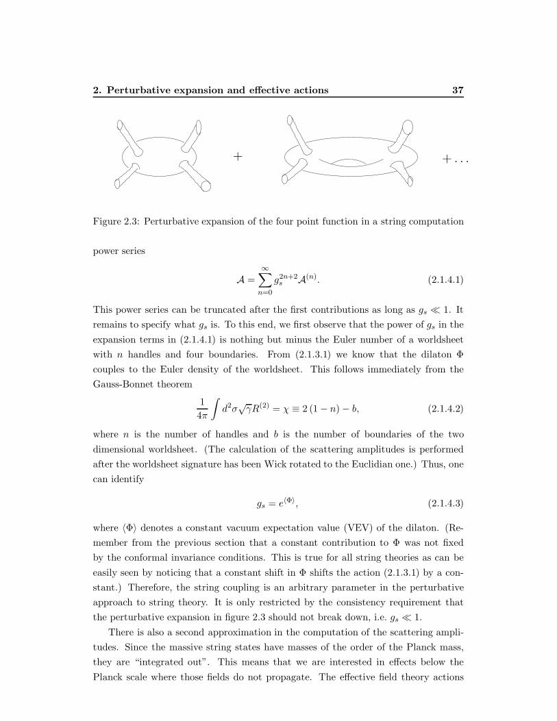
2. Perturbative expansion and effective actions 37
+ . . .+
Figure 2.3: Perturbative expansion of the four point function in a string computation
power series
A =
∞∑
n=0
g2n+2s A(n). (2.1.4.1)
This power series can be truncated after the first contributions as long as gs 1. It
remains to specify what gs is. To this end, we first observe that the power of gs in the
expansion terms in (2.1.4.1) is nothing but minus the Euler number of a worldsheet
with n handles and four boundaries. From (2.1.3.1) we know that the dilaton Φ
couples to the Euler density of the worldsheet. This follows immediately from the
Gauss-Bonnet theorem
1
4π
∫d2σ√γR(2) = χ ≡ 2 (1− n)− b, (2.1.4.2)
where n is the number of handles and b is the number of boundaries of the two
dimensional worldsheet. (The calculation of the scattering amplitudes is performed
after the worldsheet signature has been Wick rotated to the Euclidian one.) Thus, one
can identify
gs = e〈Φ〉, (2.1.4.3)
where 〈Φ〉 denotes a constant vacuum expectation value (VEV) of the dilaton. (Re-
member from the previous section that a constant contribution to Φ was not fixed
by the conformal invariance conditions. This is true for all string theories as can be
easily seen by noticing that a constant shift in Φ shifts the action (2.1.3.1) by a con-
stant.) Therefore, the string coupling is an arbitrary parameter in the perturbative
approach to string theory. It is only restricted by the consistency requirement that
the perturbative expansion in figure 2.3 should not break down, i.e. gs 1.
There is also a second approximation in the computation of the scattering ampli-
tudes. Since the massive string states have masses of the order of the Planck mass,
they are “integrated out”. This means that we are interested in effects below the
Planck scale where those fields do not propagate. The effective field theory actions
2. Perturbative expansion and effective actions 38
contain only the massless modes. For consistency, one should then restrict to processes
where the momentum transfer is p2 1/α′.
The (bosonic part of the) effective Lagrangians with at most two derivatives and
only the massless fields turn out to be
S = Suniv + Smodel, (2.1.4.4)
where Suniv does not depend on which of the superstring theories we are looking at,
and Smodel is model dependent. The universal sector has as bosonic fields the metric,
the dilaton, and the B field. The corresponding action is
Suniv =1
2κ2
∫d10x√−Ge−2Φ
(R+ 4 (∂Φ)2 − 1
12H2
), (2.1.4.5)
where κ2 ∼ (α′)4 is the ten dimensional gravitational constant. Note that the set
of equations of motion obtained from this action coincides with the conformal invari-
ance conditions (2.1.3.53)– (2.1.3.55), with the difference that for the superstring the
constant contribution in the dilaton equation vanishes for d = 10.
For type II strings there are additional contributions giving the kinetic terms for
the RR gauge forms and Chern-Simons interactions,
SIImodel = − 1
2κ2
∫d10x
∑
p
1
2(p+ 2)!F 2p+2, (2.1.4.6)
where Fp+2 is the fieldstrength of a p+ 1 form RR gauge field (plus –in some cases–
additional contributions which we will discuss later),
Fp+2 = dAp+1 + . . . . (2.1.4.7)
The number p is the spatial extension of an object which couples electrically to the
p+ 2 form gauge field. In the worldvolume action of the corresponding p dimensional
object this coupling is
∫dp+1σ iεα1···αp+1∂α1X
µ1 · · ·∂αp+1Xµp+1Aµ1 ···µp+1 . (2.1.4.8)
For a point particle (p = 0) the above expression reads for example
i
∫dτdXµ
dτAµ.
From expression (2.1.3.1) we observe that the fundamental string is electrically charged
under the NSNS B field. We will meet objects which are charged under the RR gauge
forms when discussing D-branes in section 2.3. For the type IIA theory we have

2. Perturbative expansion and effective actions 39
p = 0, 2, 4. Alternatively we could replace the field strength in (2.1.4.6) by its Hodge
dual20
F8−p = ?Fp+2. (2.1.4.9)
In the type IIA theory the definition (2.1.4.7) is modified for the four form field strength
F4 = dA3 +A1 ∧H, (2.1.4.10)
leading to a non standard Bianchi identity for the four form field strength
dF4 = F2 ∧H. (2.1.4.11)
Finally, the Chern-Simons interaction for type IIA is
SIIACS = − 1
8κ2
∫F4 ∧ F4 ∧B. (2.1.4.12)
For type IIB theories one has p = −1, 1, 3. For p = −1 the gauge form is a scalar,
which is called axion. The object which is electrically charged under this zero form is
localized in space and time. This is an instanton. The definition of the field strength
(2.1.4.7) receives further contributions for p = 1 and p = 3
F3 = dA2 − A0 ∧H, (2.1.4.13)
F5 = dA4 −1√3A2 ∧H +
1√3B ∧ F3. (2.1.4.14)
The Chern-Simons interaction for the type IIB theory is
SIIBCS = − 9
4κ2
∫A4 ∧H ∧ F3. (2.1.4.15)
The five form field strength has to be selfdual. This is not encoded in the action
(2.1.4.6) but has to be added as an additional constraint,
F5 = ?F5. (2.1.4.16)
In the heterotic string we have gauge fields transforming in the adjoint of SO(32)
or E8 × E8. Their field strength is defined as (we assign mass dimension one to the
gauge fields A – this is related to a√α′ rescaling of A)
F = dA+A ∧A. (2.1.4.17)
20This can be done by adding the Bianchi identity dFp+2 = d (· · · ) with a Lagrange multiplier tothe action and integrating out Ap+1. Because of covariance the Lagrange multiplier is a 7 − p formand its field strength is an 8− p form.
2. Perturbative expansion and effective actions 40
The definition of H in (2.1.4.5) needs to be modified21
H = dB − α′
4(ωY − ωL) . (2.1.4.18)
The Yang-Mills Chern-Simons form ωY is
ωY = trA ∧ dA+2
3trA ∧A ∧A, (2.1.4.19)
where A is the gauge connection of either E8 × E8 or SO(32). The modification
(2.1.4.18) implies that the B field transforms under gauge transformations and under
local Lorentz rotations in a non-trivial way such that H is gauge invariant. The
Yang-Mills Chern-Simons form has the property that its exterior derivative gives the
instanton density (in a four dimensional subspace with Euclidean signature),
dωY = trF ∧ F. (2.1.4.20)
The Lorentz Chern-Simons form is constructed from the spin connection ω,
dωL = trω ∧ dω +2
3trω ∧ ω ∧ ω. (2.1.4.21)
If its exterior derivative takes values only on a four dimensional submanifold with
Euclidean signature it corresponds to the Euler density of that manifold,
dωL = trR ∧ R. (2.1.4.22)
If we take the ten dimensional geometry to consist of a direct product of a six dimen-
sional non compact and a four dimensional compact space (with Euclidean signature)
the modification (2.1.4.18) implies restrictions on the allowed gauge bundles on the
four dimensional compact space. The integration of dH over a compact space should
vanish. It follows that the Euler number of this space must be equal to the instanton
number of the gauge bundle.
In addition to the universal piece (2.1.4.5), the heterotic action contains a gauge
kinetic term and also the Green-Schwarz term which ensures anomaly cancellation
Sheteroticmodel = Sgauge + SGS , (2.1.4.23)
with
Sgauge = − 1
2κ2
∫d10xe−2Φα
′
8trF 2, (2.1.4.24)
21We present the effective action for the heterotic string just for completeness, more details ondifferential geometry and anomaly cancelation in the context of the effective heterotic theory can befound e.g. in [223].

2. Perturbative expansion and effective actions 41
where again, the trace is taken over the gauge group (E8 × E8 or SO(32)). The
Green-Schwarz term is
SGS =8πi
α′
∫B ∧X8, (2.1.4.25)
with (here, a power is meant with respect to the wedge product, e.g. F 4 ≡ F∧F∧F∧F )
X8 =1
2
1
(2π)6
1
48
(5
4trF 4 − 1
8
(trF 2
)2 − 1
8trF 2trR2 +
1
8trR4 +
1
32
(trR2
)2)
(2.1.4.26)
To close this section on effective actions we identify the different contributions
with the worldsheet topologies they correspond to. First, we observe that all the
terms appearing in the effective actions are of a structure such that they contain some
power of eΦ times a factor which is invariant under constant shifts in Φ. In (2.1.4.3)
we have identified the string coupling as a constant part of eΦ. Thus, the leading term
in the perturbative expansion in figure 2.3 enters the effective action accompanied
with a factor of e−2Φ. These are all terms in (2.1.4.5) and the gauge kinetic term
in the heterotic theory (2.1.4.24). One may be tempted to interpret the other terms
(containing no e−2Φ factor) as one loop contributions. This is, however, misleading.
In order to simplify the Bianchi identities for the RR gauge forms we have rescaled
the RR gauge potentials by eΦ. Undoing this rescaling means that for example the
RR form F2 receives a further contribution
A1 = e−ΦA′1 −→ F2 = e−Φ(dA′1 − dΦ ∧A′1
)≡ e−ΦF ′2, (2.1.4.27)
and similar relations for the other RR field strengths. (If the terms denoted by dots in
(2.1.4.7) contain other RR field strengths additional Φ derivatives will be picked up.
But no relative power of eΦ will appear, since those terms always contain one RR field
strength or potential and an NSNS field strength or potential. The NSNS fields are
not rescaled.) After this rescaling all terms in the type II thoeries are of the structure
e−2Φ (invariant under Φ→ Φ + constant) .
Since the rescaled (primed) fields correspond to the actual string excitations, the
effective type II actions given here contain only tree level contributions.
As (implicitly) stated above, one loop contributions are multiplied by g2s and hence
enter the effective action with a factor of e−2Φ+2Φ = 1. In the type II examples, we
have seen that due to field redefinitions this correspondence may be changed. In
the heterotic case, however, there is no field redefinition such that all the terms in
the effective action are multiplied by the same power of eΦ. Indeed, the appearance

2. Toroidal Compactification and T-duality 42
of the Green-Schwarz term corresponds to a torus amplitude from the string theory
perspective. We excluded also higher orders in α′ which would lead to higher derivative
terms and contributions with massive string excitations.22 As long as the string scale
is much shorter (in length) than the scale of the process we are interested in those
terms can be neglected.
2.1.5 Toroidal Compactification and T-duality
In the previous sections we argued that perturbative superstring theories are consistent
provided that the target space is ten dimensional. As it stands, this cannot describe
our observable (four dimensional) world. At the end of section (2.1.3), we sketched as
a possible resolution to this problem the option to replace six of the target space di-
mensions by a conformal field theory with the desired central charge. One simple way
to do so, is to replace a six dimensional subspace of the ten dimensional Minkowski
space by a compact manifold. The coordinates of that compact manifold should be-
long to a conformal field theory with a consistent central charge. This restricts the
set of possible compactifications. The easiest option is to compactify the additional
directions on circles (by periodic identification of the corresponding coordinates). This
clearly does not change the central charge contribution of those directions, since the
central charge depends only on local features of the target space.
2.1.5.1 Kaluza-Klein compactification of a scalar field
Before discussing some details of torus compactifications of string theories we recall
the Kaluza-Klein compactification of a free massless scalar field. This will enable us
to appreciate new “stringy” features which we will study afterwards. Let us start with
a free massless scalar living in a five dimensional Minkowski space. We label the first
four coordinates with a greek index µ = 0, . . . , 3 and call the fifth direction y. The
five dimensional field equation for the scalar ϕ is
(ηµν∂µ∂ν + ∂2
y
)ϕ (xµ, y) = 0. (2.1.5.1)
Now, we compactify the fifth direction on a circle of radius R
y ≡ y + 2πR. (2.1.5.2)
Solutions to (2.1.5.1) have to respect the periodicity (2.1.5.2). Therefore, the y depen-
dent part of ϕ can be expanded into a Fourier series of periodic functions. Focusing
22An exception is the ωL correction in (2.1.4.18) and the Green Schwarz term. They can be deducedby using supersymmetry and anomaly cancellation.
2. Toroidal Compactification and T-duality 43
on the nth Fourier mode, we find
ϕn (xµ, y) = ϕn (xµ) einRy, (2.1.5.3)
with integer n, i.e. the momentum in the fifth direction is quantized. Plugging (2.1.5.3)
back into (2.1.5.1) leads to
(ηµν∂µ∂ν −m2
n
)ϕn (xµ) = 0, (2.1.5.4)
with
mn =n
R, (2.1.5.5)
i.e. the nth Fourier mode leads in the effective four dimensional description to a Klein-
Gordon field with mass (2.1.5.5). Since the general solution of (2.1.5.1) is a super-
position of all Fourier modes the four dimensional description contains an infinite
Kaluza-Klein tower of massive four dimensional fields (depending only on the xµ).
There are two limits to be discussed. The decompactification limit is R → ∞. In
this case all the Kaluza-Klein masses (2.1.5.5) vanish. The four dimensional descrip-
tion breaks down. The other limit is R → 0 (or the compactification radius becomes
much shorter than the experimental distance resolution). In this case, the KK masses
(2.1.5.5) become infinite except for n = 0. Only the massless mode survives and no
trace from the fifth dimension is left. This picture is very different in string theories
as we will see now.
2.1.5.2 The bosonic string on a circle
Even though the bosonic string is inconsistent because it contains a tachyon, we will
first study the compactification of the bosonic string on a circle. The essential stringy
properties will be visible in this toy model. We compactify the 26th coordinate (the
25th spatial direction),
x25 ≡ x25 + 2πR. (2.1.5.6)
In the point particle limit string theory is just quantum mechanics of a free relativistic
particle. The plane wave solution contains the factor eip25x25
where p25 is the center of
mass momentum in the 25th direction. This wave function should be periodic under
(2.1.5.6). This leads to a quantization condition for the center of mass momentum in
the compact direction
p25 =n
R, (2.1.5.7)
2. Toroidal Compactification and T-duality 44
with integer n (the momentum number). So far, everything is analogous to the free
scalar field discussed above. The new stringy property arises by observing that the
string can wind around the compact direction. Technically, this means that the peri-
odic boundary condition for the closed string is modified
X25 (τ, σ + π) = X25 (τ, σ) + 2πmR, (2.1.5.8)
where the integer m denotes the winding number. With this ingredients the mode
expansions (2.1.2.3) and (2.1.2.4) are
X25R =
1
2x25 +
( n
2R−mR
)σ− +
i
2
∑
k 6=0
1
kα25k e−2ikσ− , (2.1.5.9)
X25L =
1
2x25 +
( n
2R+ mR
)σ+ +
i
2
∑
k 6=0
1
kα25k e−2ikσ+
. (2.1.5.10)
Taking into account the compact direction, the mass shell condition has to be modified
in a straightforward way,
24∑
µ=0
pµpµ = −M2. (2.1.5.11)
Comparison with the constraints T++ = T−− = 0 (2.1.1.10) gives
M2 = 4( n
2R−mR
)2+ 8N − 8 = 4
( n
2R+ mR
)2+ 8N − 8 (2.1.5.12)
where we have used the result of section 2.1.2 for the normal ordering. In particular,
the level matching condition (the second equality in (2.1.5.12)) implies that
N − N = nm. (2.1.5.13)
Thus, for zero winding and momentum number the spectrum coincides with the spec-
trum of the uncompactified string (see section 2.1.2). In the massless sector we have
again a graviton, antisymmetric tensor and dilaton which are obtained from the state
αi−1αj−1 |k〉 , i, j 6= 25. (2.1.5.14)
The target space interpretation of the remaining excitations (containing creator(s) in
25th direction) is different. The two states
αi−1α25−1 |k〉 , α25
−1αi−1 |k〉 (2.1.5.15)
are target space vectors. They correspond to gauge fields of a U (1) × U (1) gauge
symmetry. Finally, the state
α25−1α
25−1 |k〉 (2.1.5.16)

2. Toroidal Compactification and T-duality 45
describes a target space scalar. The spectrum is supplemented by a Kaluza-Klein
and winding tower of additional states as n,m run through the integer numbers. An
interesting question is wether some of these additional states are massless. For massless
states the mass shell condition (2.1.5.12) reads
2N − 2 +( n
2R−Rm
)2= 2N − 2 +
( n
2R+ Rm
)2= 0. (2.1.5.17)
These equations can be solved for nonvanishing n or m only at special values of R.
The most interesting case is23
R2 =1
2= α′. (2.1.5.18)
One obtains the additional solutions listed in table 2.2.
n m N N
1 1 1 0
-1 -1 1 0
1 -1 0 1
-1 1 0 1
2 0 0 0
-2 0 0 0
0 2 0 0
0 -2 0 0
Table 2.2: Each line in this table gives a configuration of winding, momentum andoccupation numbers leading to massless states at R2 = 1
2 .
Each of the first four states in table 2.2 contains one creator. This gives four
additional massless vectors (if the creator points into a non-compact direction) and four
massless scalars (if the creator points into the 25th direction). The latter four states
in table 2.2 correspond to massless scalars. Together with (2.1.5.15) and (2.1.5.16) we
have six vectors and nine scalars. The vectors combine into an SU(2)× SU(2) gauge
field whereas the scalars form a (3, 3) representation. For the special value (2.1.5.18)
the gauge group U (1)× U (1) is enhanced to the non-abelian group SU (2)× SU (2).
The rank of the gauge group is not changed.
An immediate question is: what is so special about (2.1.5.18)? To answer this, we
rewrite (2.1.5.12) in a suggestive way
M2 = 4N + 4N − 8 +n2
R2+ 4m2R2, (2.1.5.19)
23Later, in section 2.2.1, we will also discus the case R2 = 2, where less states become massless.
2. Toroidal Compactification and T-duality 46
where we already aplied (2.1.5.13). We observe that the spectrum is invariant under
n↔ m and R↔ α′
R. (2.1.5.20)
Recall that in the previous equations we have set α′ = 1/2. The symmetry (2.1.5.20)
is called T-duality. Winding and momentum numbers are interchanged and simulta-
neously the compactification radius is inverted. If R takes the value (2.1.5.18), the
spectrum is invariant under interchanging winding with momentum. This radius is
called the selfdual radius. Because of the symmetry (2.1.5.20) we can restrict the
compactifications to radii equal or larger than (2.1.5.18). This is an important differ-
ence to the point particle discussed in the previous section. To make this difference
clearer let us take the compactification radius to zero. All the Kaluza-Klein momenta
diverge and only states with n = 0 survive. This is similar to the point particle case.
On the other hand, all winding states degenerate. In order to make sense out of
this situation one can apply the T-duality tranformation (2.1.5.20). But then R = 0
leads to the decompactification limit and we are back at the 26 dimensional string.
Therefore, in string theory there are always traces of compact dimensions left.
Compactifying the string on a D dimensional torus, the above considerations lead
to a ZD2 symmetry in a straightforward way. However, combining the T-duality along
circles with basis redefinitions of the torus lattice and integer shifts in the internal B
field leads to an enhancement of the T-duality group to SO (D,D,Z).
2.1.5.3 T-duality in non trivial backgrounds
In this section we will argue that the above described T-dualiy is also a symmetry for
non-trivial background configurations. We closely follow[392]. Our starting point is
the non-linear sigma model (2.1.3.1). Compactification of one target space dimension
is possible if the sigma model is invariant under constant shifts in this direction. For
the first term in (2.1.3.1) this implies that the tangent to the compactified direction
is a Killing vector. The second term is invariant provided that the Lie derivative of
Bµν in the Killing direction is an exact two-form. For the last term to be invaraint
the Lie derivative of the dilaton Φ must vanish. We now choose coordinates such that
the isometry is represented by a translation in the d− 1 direction
Xd−1 → Xd−1 + c. (2.1.5.21)
We call the other coordinates X i. The previously mentioned conditions on Bµν and
Φ imply that those fields are independent of Xd−1 (up to gauge transformations).
The next step is to gauge the symmetry (2.1.5.21) and to “undo” this by constrain-
ing the gauge fields to be of pure gauge. The constraint is implemented with the help

2. Toroidal Compactification and T-duality 47
of a Lagrange multiplier λ which finally will replace Xd−1 in the T-dual model. We
introduce two dimensional gauge fields Aα changing under (2.1.5.21) as
Aα → Aα − ∂αc, (2.1.5.22)
and replace
∂αXd−1 → DαX
d−1 ≡ ∂αXd−1 +Aα. (2.1.5.23)
Together with the above mentioned constraint (implemented by a Lagrange multiplier)
this amounts to adding to (2.1.3.1) (for simplicity we choose γαβ = ηαβ)24 a term
SA = − 1
4πα′
∫d2σ (Gd−1,d−1AαA
α + 2Gd−1,νAα∂αX
ν
+2εαβBd−1,νAα∂βXν + 2λεαβ∂αAβ
). (2.1.5.24)
Integrating over λ will result in the constraint of vanshing field strength for the Aα
which in turn imposes
Aα = ∂αϕ, (2.1.5.25)
with ϕ being a worldsheet scalar. Shifting Xd−1 by ϕ gives back the original sigma
model (2.1.3.1). Thus, adding (2.1.5.24) does not change anything. However, there
is a subtlety here. Compactifying the d − 1 direction means that we identify Xd−1
with Xd−1 + 2π (this time we put the compactification radius into the target space
metric). In order to be able to absorb ϕ intoXµ, ϕ should respect the same periodicity.
This can be ensured as follows. We continue the worldsheet to Euclidean signature
and study the sigma model for a torus worldsheet. Then we can assign two winding
numbers (corresponding to the two cycles of the torus) to the Lagrange multiplier
λ. Summing over these winding numbers (in a path integral approach) will impose
the required periodicity on the gauge fields Aα. Going through the details of this
prescription leads to the conclusion that the λ “direction” is compact λ ≡ λ+ 2π.
Instead of integrating out λ (to check that we did not change the model) we can
integrate out Aα. (Since Aα is not a propagating field this can be done by solving the
equations of motion. As well, one can integrate out Aα in a path integral, which is
Gaussian.) This procedure leads us to a dual model
S = − 1
4πα′
∫d2σ
(√−γγαβGµν∂αXµ∂βXν + εαβBµν∂αX
µ∂βXν)
− 1
4π
∫d2σ√−γΦR(2). (2.1.5.26)
24For the Minkowskian worldsheet signature the i in front of the Bµν coupling in (2.1.3.1) is replacedby one.

2. Toroidal Compactification and T-duality 48
The set of dual coordinates isXµ
=λ,X i
, and the dual background fields are,
Gd−1,d−1 =1
Gd−1,d−1, Gd−1,i =
Bd−1,i
Gd−1,d−1, (2.1.5.27)
Gij = Gij −Gi,d−1Gd−1,j +Bi,d−1Bd−1,j
Gd−1,d−1, (2.1.5.28)
Bd−1,i =Gd−1,i
Gd−1,d−1, Bij = Bij +
Gi,d−1Bd−1,j +Bi,d−1Gd−1,j
Gd−1,d−1. (2.1.5.29)
To find the dual expression for the dilaton is a bit more complicated. One can compute
Φ in a perturbative way. To this end, one requires that Φ is such that the conformal in-
variance conditions (2.1.3.53), (2.1.3.54), (2.1.3.55) are satisfied whenever the original
background satisfies them. This leads to the following formula for the dual dilaton
e−2Φ√−G = e−2Φ
√−G. (2.1.5.30)
From a path integral perspective the dilaton transformation can be motivated as fol-
lows. The path integral measure for the Xµ is covariant with respect to the metric
Gµν . In the dual model one would naturally use a measure which is covariant with re-
spect to the dual metric Gµν . The change of the measure introduces a Jacobian which
leads to (2.1.5.30). To our knowledge this is a rather qualitative statement which is
difficult to prove explicitly.
To make contact with the simple case discussed in the previous section we should
take Gd−1,d−1 = R2/α′, Gij = ηij , Bµν = 0 and Φ = const. Then the T-duality
formulæ (especially (2.1.5.27)) imply that the compactification radius is inverted. The
dilaton receives a constant shift and nothing else changes. This dilaton shift was not
visible in the discussion of the previous section. On the other hand, in the present
section we did neither see that T-duality interchanges winding with momentum nor
that there is an enhancement of gauge symmetry at the selfdual radius, because we
did not study the spectrum of the general string theory.
2.1.5.4 T-duality for superstrings
In extending the discussion of section 2.1.5.2 to the superstring we will be sketchy
and omit the technical details. Most of the statements from section 2.1.5.2 can be
directly taken over to the superstring. In the Ramond sector, some new ingredients
occur. First, we consider the type II superstring. Instead of the 26th direction we
compactify the tenth direction. Combining the T-duality transformation (2.1.5.20)
with the mode expansions (2.1.5.9) and (2.1.5.10) one realizes that (2.1.5.20) can be

2. Toroidal Compactification and T-duality 49
achieved by assigning X9 = X9L − X9
R, instead of X9 = X9L + X9
R, or equivalently
change
(right movers) −→ − (right movers) (2.1.5.31)
while keeping the original prescription of combining left with right movers. Carrying
this prescription over to the fermionic sector we observe that in the right moving
Ramond sector (see (2.1.2.58) for the definition)
(−)F −→ − (−)F . (2.1.5.32)
This in turn implies that the T-duality transformation takes us from the type IIA
to type IIB string and vice versa. Hence, T-duality is not a symmetry in type II
superstrings but relates the type IIA string with type IIB. (This is true, whenever we
perform T-duality in an odd number of directions.) The type IIA string compactified
on a circle with radius R is equivalent to the type IIB string compactified on a circle
with radius α′/R. This is consistent with the observation that the massless spectra of
circle compactified type IIA and type IIB theories are identical as depicted in table
2.3, where µ, ν = 0, . . . , 8.
NS-NS R-R
IIA Gµν , Bµν , Φ, Gµ9, Bµ9 Aµ, A9, Cµνρ , Cµν9
IIB Gµν , Bµν , Φ, Gµ9, Bµ9 B′µ9, Φ′, Cµνρ9, B′µν
Table 2.3: Massless type II fields in nine dimensions
In order to discuss compactifications of the heterotic string, it is useful to employ
a formulation where the additional 32 left moving fermions are bosonized into 16 left
moving bosonic degrees of freedom. We will not carry out this construction here.
It can be found in the books listed in section 6.1.1. The result which is of interest
in the current context is that those 16 left moving bosons are compactified on an
even selfdual lattice25. That is, that even without further compactifications from
ten to less dimensions the heterotic string contains already a left-right asymmetric
compactification. The theory does not depend on changing the basis of the ‘internal’
lattice. Compactifying the tenth dimension one observes another new feature which
is present in the heterotic string. In the previously discussed cases, there was one
modulus in circle compactfications, viz. the radius of the circle. For the heterotic
string we have 16 more moduli. These are called Wilson lines. They arise from the
25There exist exactly two such lattices Γ8 × Γ8 and Γ16 giving rise to the E8 × E8 and the SO(32)string, respectively.
2. Orbifold fixed planes 50
possibility that the non-abelian gauge fields can take constant vacuum expectation
values (vev) in the Cartan subalgebra of the gauge group. The fact that (at least) one
of the ten directions has been compactified is important here. Otherwise, a constant
vev could be gauged away. To see this explicitly, let us assume that the gauge field
vev is (proportional to a generator in the Cartan subalgebra)
A9 =Θ
R= e−
x9ΘR ∂9e
x9ΘR , (2.1.5.33)
where the second part of the equation shows that a constant vev is a pure gauge
configuration. However, in the compact case we have identified x9 with x9 + 2πR and
hence only gauge transformations which are periodic under this shift are allowed. This
implies that the Wilson line (2.1.5.33) can be gauged away only if Θ is an integer. From
this discussion it follows that generically the gauge group is broken to U(1)16 in the
compactification process. In addition there are the (abelian) Kaluza-Klein gauge fields
G9µ and B9µ corresponding to a U(1)×U(1) gauge symmetry. Thus, generically there
is a U (1)18 gauge symmetry in the circle compactified heterotic string. Depending
on the moduli (Wilson lines and compactification radius) there are special points of
stringy gauge group enhancement.
It can be proven that the E8 × E8 heterotic string and the SO(32) string are
continuously connected in moduli space once they have been compactified to nine
dimensions. This can be shown by observing that for a certain configuration of Wilson
lines (where the gauge group is broken to SO(16) × SO(16) in either theory) T-
duality maps the two compactifications on each other. (For details see e.g. Polchinski’s
book[371].) All other compactifications can be reached by continuously changing the
moduli. Including the original ten dimensional theories as decompactification limits
we see that the two different heterotic strings belong to the same set of theories sitting
at different corners in moduli space. For completeness we should mention that for
compactifications of the heterotic string on a D dimensional torus one finds the T-
duality group SO (16 +D,D,Z).
2.2 Orbifold fixed planes
In the previous sections we have studied the theory of a one dimensional extended
object – the string. One of the striking features of this theory is that it automatically
also describes objects which are extended along more than one space direction. As the
simplest example we will study now the orbifold fixed planes. Here, one compactifies
the string on a torus whose lattice has a discrete symmetry, and gauges this symme-
try26. Thus, the compact manifold is a D dimensional torus divided by some discrete26With gauging of a discrete symmetry we mean that only invariant states are kept.
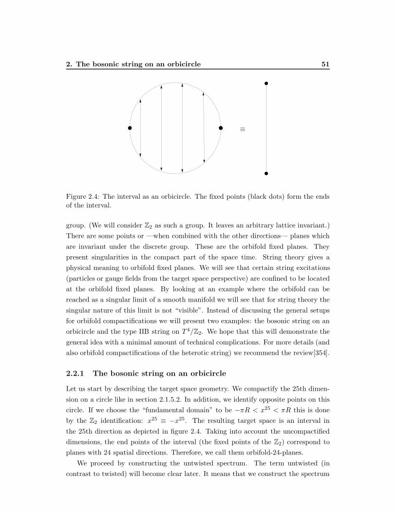
2. The bosonic string on an orbicircle 51
≡
Figure 2.4: The interval as an orbicircle. The fixed points (black dots) form the endsof the interval.
group. (We will consider Z2 as such a group. It leaves an arbitrary lattice invariant.)
There are some points or —when combined with the other directions— planes which
are invariant under the discrete group. These are the orbifold fixed planes. They
present singularities in the compact part of the space time. String theory gives a
physical meaning to orbifold fixed planes. We will see that certain string excitations
(particles or gauge fields from the target space perspective) are confined to be located
at the orbifold fixed planes. By looking at an example where the orbifold can be
reached as a singular limit of a smooth manifold we will see that for string theory the
singular nature of this limit is not “visible”. Instead of discussing the general setups
for orbifold compactifications we will present two examples: the bosonic string on an
orbicircle and the type IIB string on T 4/Z2. We hope that this will demonstrate the
general idea with a minimal amount of technical complications. For more details (and
also orbifold compactifications of the heterotic string) we recommend the review[354].
2.2.1 The bosonic string on an orbicircle
Let us start by describing the target space geometry. We compactify the 25th dimen-
sion on a circle like in section 2.1.5.2. In addition, we identify opposite points on this
circle. If we choose the “fundamental domain” to be −πR < x25 < πR this is done
by the Z2 identification: x25 ≡ −x25. The resulting target space is an interval in
the 25th direction as depicted in figure 2.4. Taking into account the uncompactified
dimensions, the end points of the interval (the fixed points of the Z2) correspond to
planes with 24 spatial directions. Therefore, we call them orbifold-24-planes.
We proceed by constructing the untwisted spectrum. The term untwisted (in
contrast to twisted) will become clear later. It means that we construct the spectrum
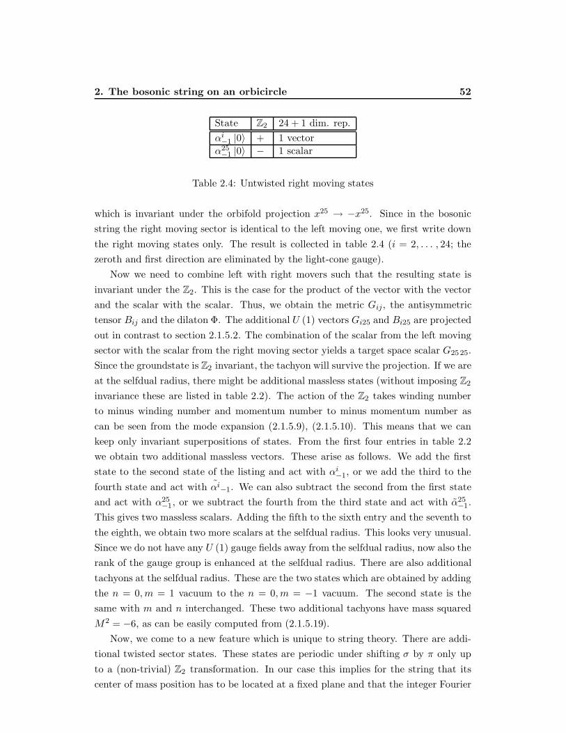
2. The bosonic string on an orbicircle 52
State Z2 24 + 1 dim. rep.
αi−1 |0〉 + 1 vector
α25−1 |0〉 − 1 scalar
Table 2.4: Untwisted right moving states
which is invariant under the orbifold projection x25 → −x25. Since in the bosonic
string the right moving sector is identical to the left moving one, we first write down
the right moving states only. The result is collected in table 2.4 (i = 2, . . . , 24; the
zeroth and first direction are eliminated by the light-cone gauge).
Now we need to combine left with right movers such that the resulting state is
invariant under the Z2. This is the case for the product of the vector with the vector
and the scalar with the scalar. Thus, we obtain the metric Gij , the antisymmetric
tensor Bij and the dilaton Φ. The additional U (1) vectors Gi25 and Bi25 are projected
out in contrast to section 2.1.5.2. The combination of the scalar from the left moving
sector with the scalar from the right moving sector yields a target space scalar G25 25.
Since the groundstate is Z2 invariant, the tachyon will survive the projection. If we are
at the selfdual radius, there might be additional massless states (without imposing Z2
invariance these are listed in table 2.2). The action of the Z2 takes winding number
to minus winding number and momentum number to minus momentum number as
can be seen from the mode expansion (2.1.5.9), (2.1.5.10). This means that we can
keep only invariant superpositions of states. From the first four entries in table 2.2
we obtain two additional massless vectors. These arise as follows. We add the first
state to the second state of the listing and act with αi−1, or we add the third to the
fourth state and act with αi−1. We can also subtract the second from the first state
and act with α25−1, or we subtract the fourth from the third state and act with α25
−1.
This gives two massless scalars. Adding the fifth to the sixth entry and the seventh to
the eighth, we obtain two more scalars at the selfdual radius. This looks very unusual.
Since we do not have any U (1) gauge fields away from the selfdual radius, now also the
rank of the gauge group is enhanced at the selfdual radius. There are also additional
tachyons at the selfdual radius. These are the two states which are obtained by adding
the n = 0, m = 1 vacuum to the n = 0, m = −1 vacuum. The second state is the
same with m and n interchanged. These two additional tachyons have mass squared
M2 = −6, as can be easily computed from (2.1.5.19).
Now, we come to a new feature which is unique to string theory. There are addi-
tional twisted sector states. These states are periodic under shifting σ by π only up
to a (non-trivial) Z2 transformation. In our case this implies for the string that its
center of mass position has to be located at a fixed plane and that the integer Fourier

2. The bosonic string on an orbicircle 53
modes are replaced by half-integer ones in the 25th direction. In the twisted sector we
need to compute the groundstate energy. This can be done by first modifying equation
(2.1.2.46) in a straightforward way
atwisted = −23
2
∞∑
n=1
n − 1
2
∞∑
r= 12
r. (2.2.1.1)
Regularizing this expression according to the prescription (2.1.2.47) gives a = 1516 .
This implies that the groundstate is tachyonic and also that there is no massless state
coming from this twisted ground state. There is one more tachyonic state at the first
level in the twisted sector. This is obtained by acting with α25− 1
2
α25− 1
2
. Collecting the
results, we obtain one tachyon with M2 = −152 and one with M2 = −7
2 at each fixed
plane. Altogether, there are four tachyons (and states with positive mass squared)
located at the fixed planes.
The singular nature of the fixed points does not raise any problem in string theory.
It introduces twisted sector states which result in additional particles which are located
at the orbifold-24-planes in target space.
It is interesting to note that the orbifold at the selfdual radius is equivalent to the
toroidally compactified bosonic string at twice the selfdual radius.27 For a detailed
disussion of this equivalence we refer to Polchinski’s book[371]. Here, we will only
check that the light (tachyonic and massless) spectra coincide. Obviously, the gauge
groups U (1)× U (1) are the same. For the bosonic string on the circle (with R2 = 2)
these are the off-diagonal metric and B-field components Gi25, Bi25, whereas for the
orbicircle compactification at R2 = 12 these come from states with non-trivial winding
and momenta as discussed above. It remains to identify the four additional massless
scalars and the two tachyons (found in the non-trivial winding-momenta sector) of the
orbicircle compactification (at selfdual radius) and the four additional tachyons from
the twisted sector in the circle compactification. Here, the special choice R2 = 2 for
the circle compactification comes into the game. With (2.1.5.19) evaluated at R2 = 2
we find exactly these missing states. At first, there are four massless scalars: the vacua
with m = 0 and n = ±4, or m = ±1 and n = 0. The two tachyons with M2 = −6 are
obtained from the two vacua with m = 0 and n = ±2. The two twisted sector tachyons
with M2 = −152 correspond to the two vacua with m = 0 and n = ±1. The other two
twisted sector tachyons with M2 = −72 can be identified in the circle compactification
as the vacua with m = 0 and n = ±3.
The equivalence of the S1/Z2 compactification at the selfdual radius and the S1
compactification at twice the selfdual radius shows that the moduli spaces of both
27Alternatively, we could use the T-dual version at half the selfdual radius.

2. Type IIB on T 4/Z2 54
x8
x9
Figure 2.5: The orbifold T 2/Z2
compactifications are connected at this point. This feature has a stringy origin. From
the target space perspective this is quite surprising. A field theory on 24 + 1 dimen-
sional Minkowski space times an interval with certain fields constrained to live at the
endpoints of the interval is smoothly connected to a field theory on 24+1 dimensional
Minkowski space times a circle with all fields living in the whole space. However, due
to the tachyons both vacua are unstable. In the next section we will see that similar
things happen for the superstring which does not have tachyons in its spectrum.
2.2.2 Type IIB on T 4/Z2
Again, we start by describing the target space geometry. We compactify the six, seven,
eight and nine direction on a four dimensional torus. We view this four dimensional
torus as the product of two two-dimensional tori. The coordinates are labeled such
that the sixth and seventh direction form one T 2 and the eighth and ninth a second
T 2. Let us focus on this second T 2 with the understanding that the same applies to the
first T 2. In figure 2.5 this is depicted by drawing a lattice in the eight-nine plane. The
fundamental cell is the parallelogram with edges drawn with stronger lines. The lattice
vectors are the lower and the left edge of the fundamental cell. A two dimensional
torus is obtained by gluing together the opposite edges of the fundamental cell. Shifts
by lattice vectors connect identified points.
“Dividing” the T 4 by Z2 means that in addition we identify points via the pre-
scription
x6, x7, x8, x9
→−x6,−x7,−x8,−x9
. (2.2.2.1)
This Z2 action leaves the four points indicated by black dots in figure 2.5 times the
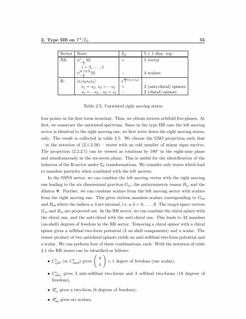
2. Type IIB on T 4/Z2 55
Sector State Z2 5 + 1 dim. rep.
NS: ψi− 12
|0〉 + 1 vector
i = 2, . . . , 5
ψ6,7,8,9
− 12
|0〉 − 4 scalars
R: |s1s2s3s4〉 eiπ2
(s3+s4)
s1 = s2, s3 = −s4 + 2 (anti-chiral) spinorss1 = −s2 , s3 = s4 − 2 (chiral) spinors
Table 2.5: Untwisted right moving states
four points in the first torus invariant. Thus, we obtain sixteen orbifold five-planes. At
first, we construct the untwisted spectrum. Since in the type IIB case the left moving
sector is identical to the right moving one, we first write down the right moving states,
only. The result is collected in table 2.5. We choose the GSO projection such that
—in the notation of (2.1.2.56)— states with an odd number of minus signs survive.
The projection (2.2.2.1) can be viewed as rotations by 180 in the eight-nine plane
and simultaneously in the six-seven plane. This is useful for the identification of the
behavior of the R-sector under Z2 transformations. We consider only states which lead
to massless particles when combined with the left movers.
In the NSNS sector, we can combine the left moving vector with the right moving
one leading to the six dimensional graviton Gij , the antisymmetric tensor Bij and the
dilaton Φ. Further, we can combine scalars from the left moving sector with scalars
from the right moving one. This gives sixteen massless scalars corresponding to Gab
and Bab where the indices a, b are internal, i.e. a, b = 6, . . . , 9. The target space vectors
Gia and Bia are projected out. In the RR sector, we can combine the chiral spinor with
the chiral one, and the anti-chiral with the anti-chiral one. This leads to 32 massless
(on-shell) degrees of freedom in the RR sector. Tensoring a chiral spinor with a chiral
spinor gives a selfdual two-form potential (3 on shell components) and a scalar. The
tensor product of two antichiral spinors yields an anti-selfdual two-form potential and
a scalar. We can perform four of those combinations, each. With the notation of table
2.1 the RR states can be identified as follows:
• C∗ijkl (or C∗abcd) gives
(4
4
)= 1 degree of freedom (one scalar),
• C∗abij gives 3 anti-selfdual two-forms and 3 selfdual two-forms (18 degrees of
freedom),
• B′ij gives a two-form (6 degrees of freedom),
• B′ab gives six scalars,
2. Type IIB on T 4/Z2 56
• Φ′ gives a scalar .
All other fields from the RR sector are projected out. Fermionic degrees of freedom
are obtained from the NSR and RNS sector. Combing the vector with the anti-chiral
spinors gives four times28a (2, 2) ⊗ (2, 1) = (3, 2) ⊕ (1, 2) representation of the six
dimensional little group SO (4) = SU (2) × SU (2).29 Therefore, this tensor product
provides us with four chiral gravitini and four chiral fermions.
Combining the NS sector scalars with the chiral R sector spinors gives 16 chiral
spinors. From the existence of the four chiral gravitini we can guess that the resulting
low energy effective field theory has N = 4 chiral supersymmetry in six dimensions.
(For a collection of supersymmetries in various dimension see[399].)
Before checking that also the rest of the massless states fit into supersymmetric
multiplets we should construct the twisted sector states. The construction does not
depend on the location of the fixed plane. Therefore, we restrict the construction
to one plane and multiply the result by 16. In the twisted sector, the NS fermions
with an index corresponding to a compact dimension are integer modded whereas the
R sector fermions are half integer modded. Now, there are NS sector zero modes
forming a four dimensional Clifford algebra. The twisted NS ground state is two-fold
degenerate after imposing the GSO projection. (We modify the notation of (2.1.2.56)
in a straightforward way. Since we have only two creators and two anihilators, the
twisted NS groundstate has two entries. Performing the GSO projection means that
we keep those states with an odd number of minus signs.) In the twisted R sector
we do not have zero modes in the compact direction. This lifts some of the vacuum
degeneracy as compared to the untwisted sector. The twisted R ground state is labeled
only by the first two entries. Again, we keep only states with an odd number of minus
signs. In order to deduce the masses of the states in the twisted NS sector, we observe
from (2.1.2.46) (and its regularisation) that replacing four integer moded bosons by
half integer moded ones changes the normal ordering constant by − 424 − 4
16 = − 512 .
Changing the modding of four worldsheet fermions from half-integer to integer gives
another shift of − 416 + 4
24 = − 112 . Thus, we arrive at
atwistedNS = auntwistedNS − 1
2= 0. (2.2.2.2)
The twisted NS sector groundstate is massless. The R sector groundstate is always
massless, since fermions have the same modding as bosons. The analogon of table
2.5 for the twisted sector is table 2.6. Since all the twisted sector groundstates are
28One factor of two arises because the NSR and RNS sector yield such a tensor product, each. Thesecond factor of two is due to the two anti-chiral spinors in table 2.5.
29A vector is in the (2,2), an anti-chiral spinor in the (2,1), a chiral spinor in the (1,2), a selfdualtwoform in the (3,1) and an anti-selfdual twoform in the (1,3).
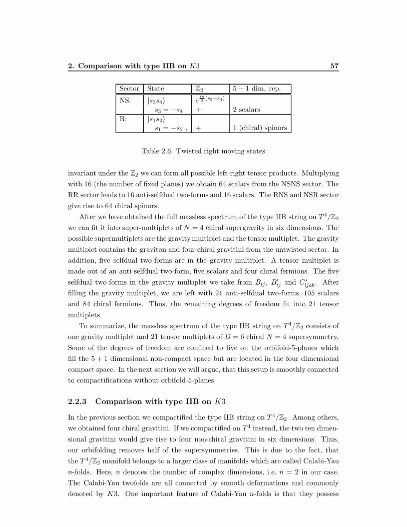
2. Comparison with type IIB on K3 57
Sector State Z2 5 + 1 dim. rep.
NS: |s3s4〉 eiπ2
(s3+s4)
s3 = −s4 + 2 scalars
R: |s1s2〉s1 = −s2 , + 1 (chiral) spinors
Table 2.6: Twisted right moving states
invariant under the Z2 we can form all possible left-right tensor products. Multiplying
with 16 (the number of fixed planes) we obtain 64 scalars from the NSNS sector. The
RR sector leads to 16 anti-selfdual two-forms and 16 scalars. The RNS and NSR sector
give rise to 64 chiral spinors.
After we have obtained the full massless spectrum of the type IIB string on T 4/Z2
we can fit it into super-multiplets of N = 4 chiral supergravity in six dimensions. The
possible supermultiplets are the gravity multiplet and the tensor multiplet. The gravity
multiplet contains the graviton and four chiral gravitini from the untwisted sector. In
addition, five selfdual two-forms are in the gravity multiplet. A tensor multiplet is
made out of an anti-selfdual two-form, five scalars and four chiral fermions. The five
selfdual two-forms in the gravity multiplet we take from Bij , B′ij and C∗ijab. After
filling the gravity multiplet, we are left with 21 anti-selfdual two-forms, 105 scalars
and 84 chiral fermions. Thus, the remaining degrees of freedom fit into 21 tensor
multiplets.
To summarize, the massless spectrum of the type IIB string on T 4/Z2 consists of
one gravity multiplet and 21 tensor multiplets of D = 6 chiral N = 4 supersymmetry.
Some of the degrees of freedom are confined to live on the orbifold-5-planes which
fill the 5 + 1 dimensional non-compact space but are located in the four dimensional
compact space. In the next section we will argue, that this setup is smoothly connected
to compactifications without orbifold-5-planes.
2.2.3 Comparison with type IIB on K3
In the previous section we compactified the type IIB string on T 4/Z2. Among others,
we obtained four chiral gravitini. If we compactified on T 4 instead, the two ten dimen-
sional gravitini would give rise to four non-chiral gravitini in six dimensions. Thus,
our orbifolding removes half of the supersymmetries. This is due to the fact, that
the T 4/Z2 manifold belongs to a larger class of manifolds which are called Calabi-Yau
n-folds. Here, n denotes the number of complex dimensions, i.e. n = 2 in our case.
The Calabi-Yau twofolds are all connected by smooth deformations and commonly
denoted by K3. One important feature of Calabi-Yau n-folds is that they possess
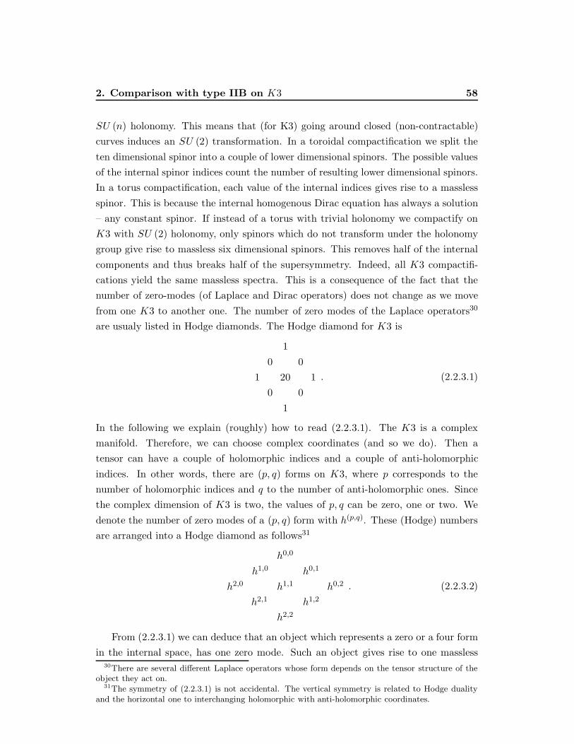
2. Comparison with type IIB on K3 58
SU (n) holonomy. This means that (for K3) going around closed (non-contractable)
curves induces an SU (2) transformation. In a toroidal compactification we split the
ten dimensional spinor into a couple of lower dimensional spinors. The possible values
of the internal spinor indices count the number of resulting lower dimensional spinors.
In a torus compactification, each value of the internal indices gives rise to a massless
spinor. This is because the internal homogenous Dirac equation has always a solution
– any constant spinor. If instead of a torus with trivial holonomy we compactify on
K3 with SU (2) holonomy, only spinors which do not transform under the holonomy
group give rise to massless six dimensional spinors. This removes half of the internal
components and thus breaks half of the supersymmetry. Indeed, all K3 compactifi-
cations yield the same massless spectra. This is a consequence of the fact that the
number of zero-modes (of Laplace and Dirac operators) does not change as we move
from one K3 to another one. The number of zero modes of the Laplace operators30
are usualy listed in Hodge diamonds. The Hodge diamond for K3 is
1
0 0
1 20 1
0 0
1
. (2.2.3.1)
In the following we explain (roughly) how to read (2.2.3.1). The K3 is a complex
manifold. Therefore, we can choose complex coordinates (and so we do). Then a
tensor can have a couple of holomorphic indices and a couple of anti-holomorphic
indices. In other words, there are (p, q) forms on K3, where p corresponds to the
number of holomorphic indices and q to the number of anti-holomorphic ones. Since
the complex dimension of K3 is two, the values of p, q can be zero, one or two. We
denote the number of zero modes of a (p, q) form with h(p,q). These (Hodge) numbers
are arranged into a Hodge diamond as follows31
h0,0
h1,0 h0,1
h2,0 h1,1 h0,2
h2,1 h1,2
h2,2
. (2.2.3.2)
From (2.2.3.1) we can deduce that an object which represents a zero or a four form
in the internal space, has one zero mode. Such an object gives rise to one massless30There are several different Laplace operators whose form depends on the tensor structure of the
object they act on.31The symmetry of (2.2.3.1) is not accidental. The vertical symmetry is related to Hodge duality
and the horizontal one to interchanging holomorphic with anti-holomorphic coordinates.
2. Comparison with type IIB on K3 59
six-dimensional field. A p + q = 2 form possesses 22 zero modes, thus leading to 22
massless fields in six dimensions. In order to write down the massless spectrum of
the K3 compactified type IIB string we need to know another feature of the family of
K3 manifolds. All Calabi-Yau manifolds (and in particular K3) are Ricci flat. This
means that the Ricci tensor vanishes and hence we do not need any non-trivial back-
ground configuration in order to satisfy the conformal invariance conditions derived in
section 2.1.3. This remains true under certain deformations of the metric of K3. The
space of such non-trivial (not related to coordinate changes) metric deformations is 58
dimensional for the family of K3s.
Now, we are ready to derive the bosonic massless spectrum of the K3 compactified
type IIB string. At first, we collect all zero forms of K3. From the NSNS sector these
are Gij ,Bij ,Φ, and from the RR sector B′ij , Φ′, C∗ijkl. Since h(0,0) = 1 these appear
once in the lower dimensional spectrum. The Gab are not differential forms on K3 but
metric deformations. They result in 58 massless scalars. Since h(p,q) = 0 for p+q odd,
the Kaluza-Klein fields Gia and Bia do not give rise to massless six dimensional fields.
It remains to count the two-forms on K3. (The four form C∗abcd we have already
counted as C∗ijkl because of selfduality.) The two-forms are Bab, B′ab and C∗ijab. Bab
and B′ab lead to 44 scalars in six dimensions. The 22 zero-modes of C∗ijab can be
decomposed into three selfdual and 19 anti-selfdual twoforms in six dimensions[38].
Taking into account that the SU(2) holonomy breaks half of the supersymmetry (as
compared to T 4 compactifications) and that the fermionic zero modes are all of the
same chirality, we obtain the same massless spectrum as in the T 4/Z2 case.
Indeed, T 4/Z2 corresponds to a limit in the space of K3 manifolds where the K3
degenerates. As long as one considers K3s very close to that point one obtains the
same massless spectrum. In string theory even the limit to the point where the K3
degenerates is well defined.
Let us see what happens when we repeat theK3 analysis for the orbifold T 4/Z2. We
will focus only on the bosonic spectrum. First, we need to know the Hodge diamond for
T 4/Z2. This can be easily “computed” without much knowledge of algebraic geometry.
On T 4 we obtain the Hodge numbers just by counting independent components of the
corresponding differential forms,
hp,q =
(2
p
)(2
q
). (2.2.3.3)
The Z2 action is taken into account by removing forms which are odd under the Z2.

2. Comparison with type IIB on K3 60
Thus, the Hodge diamond for T 4/Z2 is
1
0 0
1 4 1
0 0
1
. (2.2.3.4)
In six dimensions we obtain two twoforms Bij and B′ij and three scalars Φ, Φ′, C∗ijkl.
The internal metric components Gab yield ten scalars. (Note, that constant rescal-
ings of the coordinates would change the range of those coordinates, and hence are
non-trivial deformations equivalent to a constant change of the corresponding metric
components.) From the metric deformations we obtain 48 less scalars than in the K3
compactification. It remains to take into account the twoforms on T 4/Z2: Bab, B′ab
and C∗ijab. We obtain 12 massless scalars from Bab and B′ab, together. On the K3 there
were 32 more massless scalars coming from this sector. The C∗ijab combine into three
selfdual and three anti-selfdual twoforms. In the K3 compactification we obtained 16
more anti-selfdual two-forms.
The T 4/Z2 spectrum we computed here, would correspond to the one which we
had obtained in a field theory compactification. It has 80 massless scalars and 16
anti-selfdual twoforms less than the K3 compactified theory. In field theory, the spec-
trum jumps when we take the singular orbifold limit in the family of K3s. From the
above construction it is obvious that we counted only untwisted states from a string
perspective. Indeed, the missing 80 scalars and 16 anti-selfdual twoforms are exactly
what we obtained from the twisted sector in the previous section. In string theory the
spectrum of the compactified theory does not feel the singular nature of the orbifold
limit. All that happens is that some part of the spectrum is localized to the orbifold
fixed planes. This localization appears in internal space and is not visible at exper-
iments which cannot resolve the distances of the size of the compact manifold. The
energy scale of such experiments depends on the type of interactions fields propagating
into the compact directions carry. For purely gravitational interactions it needs to be
much higher than e.g. for electro-magnetic interactions. We will come back to this
later.
To summarize we recall that string theory can be compactified on singular mani-
folds. The moduli spaces of such compactifications can be connected to compactifica-
tions on smooth manifolds. There are massless states which are localized at singular-
ities of the compact manifold. These are the twisted sector states. They are of truly
stringy origin.

2. D-branes 61
2.3 D-branes
In this section we will present another kind of extended objects resulting from string
theory — the D-branes. They are different from the previously studied orbifold planes.
D-branes can exist also in uncompactified theories. They are dynamical objects, i.e.
they interact with each other and can move independent of the size of some compact
space. (The orbifold planes could move only if we changed the size or shape of the
compact manifold.) When we discussed the fundamental string we did not consider
the possibility of open strings. We will catch up on that in the following.
2.3.1 Open strings
2.3.1.1 Boundary conditions
We recall the action of the superstring
S =1
2πα′
∫dσ+dσ−
(∂−X
µ∂+Xµ +i
2ψµ+∂−ψ+µ +
i
2ψµ−∂+ψ−µ
). (2.3.1.1)
Now, we view the values σ = 0, π as true boundaries of the string worldsheet. Varying
(2.3.1.1) with respect to Xµ gives apart from the equations of motion (which are
identical to closed strings) boundary terms which should vanish separately,
δXµ∂σXµ|πσ=0 = 0. (2.3.1.2)
For the closed string we have solved this equation by relating the values at σ = 0 with
the ones at σ = π. This procedure was local because we took the string to join to a
closed string at σ = π. Now, we proceed differently by not correlating the two ends of
the string, i.e.
δXµ∂σXµ|σ=0 = δXµ∂σXµ|σ=π = 0. (2.3.1.3)
Let us focus on the boundary at σ = 0. We have two choices to satisfy the boundary
condition. If —for i = 0, . . . , p— we allow for free varying ends (δX i arbitrary at the
boundary) we obtain Neumann boundary conditions at those ends32
∂σXi = 0 , i = 0, . . . , p. (2.3.1.4)
For the remaining d− p− 1 coordinates Xa we choose to freeze the end of the string
— the variation vanishes at the boundary. Hence, in those directions the end of the
string is confined to some constant position. The resulting boundary conditions are
Dirichlet conditions (ca is a constant vector),
Xa = ca , a = p+ 1, . . . , d. (2.3.1.5)
32Here, we use i to label Neumann directions. After fixing the light cone gauge we take i = 2, . . . , p.
2. Open strings 62
The end of the open string defines a surface which extends along p+ 1 dimensions and
is located in d− p− 1 dimensions. This object is called D-brane, where the “D” refers
to the Dirichlet boundary condition specifying its position. If we choose identical
boundary conditions for the other end of the open string (at σ = π), we describe
an open string starting and ending on the same D-brane. For different boundary
conditions the open string stretches between two different D-branes. The Neumann
conditions imply that no momentum can flow out of the ends of the open string. In the
Dirichlet directions momentum can leave the string through its end — it is absorbed
by the D-brane. The target space Lorentz group is broken to SO(p, 1).
Varying the action with respect to the worldsheet fermions results in the same
equations of motions as in the closed string case and in the boundary conditions
(−ψ+µδψ
µ+ + ψ−µδψ
µ−)∣∣πσ=0
= 0. (2.3.1.6)
In the closed string case we have solved this by assigning either periodic or anti-
periodic boundary conditions to the worldsheet fermions. Since now the ends of the
string are separated in the target space this would imply some non-locality. Therefore,
we impose the boundary conditions (2.3.1.6) at each end separately
(−ψ+µδψ
µ+ + ψ−µδψ
µ−)∣∣σ=0
=(−ψ+µδψ
µ+ + ψ−µδψ
µ−)∣∣σ=π
= 0. (2.3.1.7)
Let us focus again on the boundary at σ = 0. We can solve (2.3.1.7) by one of the
options
ψµ+ = ±ψµ− at σ = 0. (2.3.1.8)
However, there is a correlation with the bosonic boundary conditions via worldsheet
supersymmetry. To be specific, we choose the plus sign for Neumann conditions
ψi+ = ψi− at σ = 0. (2.3.1.9)
The supersymmetry transformations (in particular (2.1.1.22) and (2.1.1.23)) should
not change this boundary condition. Since ∂τXi is not specified by the boundary
conditions this yields
ε+ = −ε− at σ = 0, (2.3.1.10)
which implies that due to the boundary (at least) half of the worldsheet supersymmetry
is broken. (If we had started with (1, 0) worldsheet supersymmetry —as we did for the
heterotic string— the boundary would break worldsheet supersymmetry completely.)
In order to ensure that not all of the supersymmetry is broken we have to choose
2. Open strings 63
the opposite (compared to (2.3.1.9)) boundary conditions for worldsheet fermions in
Dirichlet directions
ψa+ = −ψa− at σ = 0. (2.3.1.11)
We could also interchange the fermionic boundary conditions in Dirichlet and Neu-
mann directions. Then another worldsheet supersymmetry would survive. There is
no physical difference between the two choices. Nevertheless it is important, that we
take the boundary conditions in the Neumann directions to be “opposite” to the ones
in Dirichlet directions. One may also check that the open string action is invariant
under the worldsheet supersymmetries (2.1.1.20), (2.1.1.22) and (2.1.1.23) provided
that the worldsheet fermions satisfy the boundary conditions (2.3.1.9), (2.3.1.11) and
(2.3.1.10) is fulfilled. (Partial integration introduces boundary integrals which vanish
if these additional constraints hold.) Recall also that the functional form of the world-
sheet supersymmetry parameter is restricted by the chirality conditions (2.1.1.28).
In the following we are going to discuss the boundary conditions at the other end
of the open string at σ = π. Going back to the closed string we deduce from (2.1.1.22)
that for anti-periodic supersymmetry parameter ε+ the fermions are anti-periodic for
periodic bosons and vice versa. This means that anti-periodic ε+ belongs to the
NS sector and periodic ones to the R sector. From the discussion of the boundary
conditions at σ = 0 we infer that the supersymmetry parameter has to satisfy one of
the following conditions,
ε+ = ±ε− at σ = π. (2.3.1.12)
In order to relate this to something like periodicity or anti-periodicity we perform
the so called doubling trick. This means that we define a function ε on the interval
0 ≤ σ < 2π. This is done in the following way (we indicate only the σ dependence),
ε =
ε+ (σ) , 0 ≤ σ < π
±ε− (2π − σ) , π ≤ σ < 2π. (2.3.1.13)
The sign in the second line of (2.3.1.13) is correlated to the sign in (2.3.1.12) by the
requirement of continuity at σ = π. Hence, ε is (anti)-periodic for the lower (upper)
sign in (2.3.1.12) (taking into account the sign in (2.3.1.10)).
Now, let us perform this doubling trick also on the worldsheet bosons and fermions.
For the bosons it is useful to rewrite the boundary conditions. Dirichlet boundary
conditions mean that
∂+Xa = −∂−Xa at σ+ − σ− = 0. (2.3.1.14)

2. Open strings 64
Neumann conditions can be written as
∂+Xi = ∂−X
i at σ+ − σ− = 0. (2.3.1.15)
The next step is to specify the boundary conditions at σ = π. After having done this,
one can perform the doubling trick, i.e. define a boson ∂Xµ on the interval 0 ≤ σ < 2π
analogously to the definition of ε in (2.3.1.13) where ∂±X take the role of ε±. As the
reader can easily verify, the outcome is that ∂Xµ is periodic whenever we have chosen
the same type of boundary conditions at the two ends of the string in the xµ direction.
The corresponding open string sectors are called DD (NN) according to the choice of
Dirichlet (Neumann) boundary conditions at the two ends. For an opposite choice of
boundary conditions (ND or DN strings) ∂Xµ will turn out to be anti-periodic. In
analogy to the closed string we call the sector with periodic ε R sector and the one
with anti-periodic ε NS sector. For DD or NN strings this implies that in the NS
sector we take the boundary conditions at σ = π to be
ψi+ = −ψi− , ψa+ = ψa− at σ = π. (2.3.1.16)
Defining a “doubled” worldsheet fermion Ψµ in analogy to ε (where the role of ε± is
taken over by the ψµ±) we find that for DD or NN strings Ψ is anti-periodic. In the R
sector we take the boundary conditions
ψi+ = ψi− , ψa+ = −ψa− at σ = π (2.3.1.17)
and obtain periodic boundary conditions. In the above we have used that, for example,
in the R-sector periodicity of ε implies that the boundary conditions of ε± at σ = π
are identical to the ones at σ = 0. Plugging this back into the supersymmetry trans-
formations (2.1.1.22) and (2.1.1.23) evaluated at σ = π and taking into account the
boundary conditions for the bosons, we obtain the boundary conditions of the world-
sheet fermions at σ = π. This in turn determines the periodicity of Ψµ. Performing
the same procedure for ND or DN boundary conditions, one finds that Ψµ is periodic
in the NS sector and anti-periodic in the R sector whenever xµ is a direction with ND
or DN boundary conditions. The ND or DN directions are somewhat similar to the
twisted sectors we met when discussing Z2 orbifolds.
At first, we will consider only the case of a single D-brane. This means that we can
have only DD or NN boundary conditions depending on whether we are looking at a
direction transverse or longitudinal to the D-brane. Then ∂Xµ will always be periodic
and Ψµ (anti-)periodic in the (NS) R sector.

2. Open strings 65
2.3.1.2 Quantization of the open string ending on a single D-brane
The quantization of the open string is very similar to the closed superstring. In
the following we will point out the differences. At first, we solve the equations of
motion again by taking a superposition of left-moving and right-moving fields. For
the bosons, these are given in (2.1.2.3) and (2.1.2.4). The boundary conditions relate
this two solutions. (In addition, we need to replace e−2inσ± → e−inσ±
.)33 In Neumann
directions, they impose
αin = αin. (2.3.1.18)
For Dirichlet directions, we obtain a similar relation and constraints on the zero modes,
xa = ca , pa = 0 , αan = −αan. (2.3.1.19)
The general solutions for the bosonic directions read
X i = xi + piτ + i∑
n6=0
1
nαine
−inτ cosnσ, (2.3.1.20)
Xa = ca −∑
n6=0
1
nαane
−inτ sinnσ. (2.3.1.21)
The mode expansions for the NS sector fermions look as follows
ψi− =1√2
∑
r∈Z+ 12
bire−irσ− , (2.3.1.22)
ψi+ =1√2
∑
r∈Z+ 12
bire−irσ+
, (2.3.1.23)
ψa− =1√2
∑
r∈Z+ 12
bare−irσ− , (2.3.1.24)
ψa+ = − 1√2
∑
r∈Z+ 12
bare−rσ+
. (2.3.1.25)
For the R sector fermions, one obtains
ψi− =∑
n∈Zdine−inσ− , (2.3.1.26)
ψi+ =∑
n∈Zdine−inσ+
, (2.3.1.27)
ψa− =∑
n∈Zdane−inσ− , (2.3.1.28)
ψa+ = −∑
n∈Zdane−inσ+
. (2.3.1.29)
33If we had chosen the open string half as long as the closed one we would not need this replacement.

2. Open strings 66
The next step is to eliminate two directions by performing the light cone gauge. We
take this to be the time-like (Neumann) direction and a space-like Neumann direction,
which we choose to be x1.34 For the open string we have only an NS sector and
an R sector. Since the right movers are not independent from the left movers, the
right and left moving sectors do not decouple anymore. The constraints that the
expressions (2.1.1.24) – (2.1.1.27) vanish are not all independent. The zero mode part
of vanishing energy momentum tensor again yields the mass shell condition (since the
mode expansions differ by factors of two, there is a difference of a factor of four as
compared to the closed string (2.1.2.42)),
M2 = 2 (N − a) , (2.3.1.30)
where a is the normal ordering constant and the number operator N is defined in
(2.1.2.43) for the NS sector and in (2.1.2.61) for the R sector. In the NS sector the
GSO projection operator is as in (2.1.2.50) with the second factor removed. The lowest
GSO invariant states in the NS sector are
bi− 12|k〉 , ba− 1
2|k〉 , (2.3.1.31)
where we have indicated again the momentum eigenvalue of the vacuum by k. The
first set of these states transforms in the vector representation of SO(p−1) – the little
group of the unbroken Lorentz group. Hence, this state should be massless leading to
the consistency condition35
aNS =1
2. (2.3.1.32)
Like in the closed string, this translates into a condition on the number of target-space
dimensions
d = 10. (2.3.1.33)
The first states in (2.3.1.31) (with label i) form a U (1) gauge field. The states with
label a are scalars transforming in the adjoint of U (1) (here, this appears just as a
pompous way of saying that they are neutral under U(1), however, later we will discuss
34We do not consider an open string ending on a D0 brane, here. As in the case of the closedstring, it is useful to take Lorentz invariance as a guiding principle for a consistent quantization. Fora D0 brane, the Lorentz group is broken down to time reparameterizations which is too small for ourpurposes. Later, we will see that we can obtain the D0 brane by T-dualizing a higher dimensionalD-brane.
35In principle, we could combine the first states in (2.3.1.31) with one of the second states in orderto form a massive vector representation as long as p < d− 1. However, later we will see that the casep = d − 1 is related by T-duality to the other cases. With this additional ingredient it follows thatthe states in (2.3.1.31) must be massless.

2. Open strings 67
0
Spin/~
M2α′
1PHOTON
1
Figure 2.6: NS mass spectrum of the open superstring
non-abelian gauge groups where those fields are adjoints rather than singlets). Since
the center of mass position of the open string is confined to be within the world volume
of the D-brane, all the open string states correspond to target-space particles which
are confined to live on the D-brane. The NS mass-spectrum is depicted in figure 2.6.
The construction of the R sector vacuum state goes along the same lines as in
the closed string. The ten dimensional Majorana spinor decomposes into a couple of
spinors with respect to the unbroken Lorentz group SO(p, 1). We impose the GSO
projection by multiplying the states with one of the projection operators defined in
(2.1.2.59). The sign is a matter of convention. The R-vacuum is massless on its own.
It leads to target space spinors providing all fermionic degrees of freedom which are
needed to obtain the maximal rigid supersymmetry in p+ 1 dimensions.36
In the following sections we will investigate systems with more than one D-brane.
This will lead to non-abelian field theories on a stack of D-branes. But before doing
so, we will briefly discuss the possible D-brane setups which are in agreement with
supersymmetry.
2.3.1.3 Number of ND directions and GSO projection
At first, consider the case that we have an open string with an odd number of ND
directions. Thus, we will have an odd number of directions where the worldsheet
36The maximally possible amount of supersymmetry differs for rigid and local supersymmetry. Inrigid supersymmetry, the highest occurring spin should not exceed one, whereas in locally supersym-metric field theories, spin two fields (the gravitons) are allowed. In 3 + 1 dimensions, the maximalsupersymmetry is N = 4 (N = 8) for rigid (local) supersymmetry. From this one can deduce themaximally allowed amount of supersymmetry in higher dimensions by viewing the 3 + 1 dimensionaltheory as a toroidally compactified higher dimensional theory.

2. Open strings 68
fermions have zero-modes. For example in the R sector, the zero-modes form a Clifford
algebra in p+1 = odd dimensions. The representation of this algebra by the R ground
state will be irreducible (there is no notion of chirality in odd dimensions). Therefore,
we cannot perform the GSO projection on those states. The theory will not lead to
target-space supersymmetry.
Let us now discuss the case of an even number of ND directions, taken to be 8−2n.
Then the GSO projection operator on the R sector ground state will be of the form
PGSO = 1± 2n d20 . . .d
2n+10 . (2.3.1.34)
Using some algebra this can be written as
PGSO = 1± eiπ(J23+...+J2n,2n+1 ), (2.3.1.35)
where the Jkl are the generators of rotations in the kl plane
Jkl = − i2
[dk0, d
l0
]. (2.3.1.36)
The eigenvalue of the ND Ramond groundstate under a 180 rotation in one plane is
±i. Thus, the eigenvalues of the R groundstate |R〉 under PGSO will be
PGSO |R〉 = (1± in) |R〉 . (2.3.1.37)
From this we deduce that the GSO projection is possible only if the number of ND
directions is an integer multiple of four. This means for example that, if a lower
dimensional D-brane lives inside the worldvolume of a higher dimensional D-brane,
the higher dimensional D-brane has to extend in four or eight more directions. We
could have deduced this result faster by noting that (2.3.1.34) defines a projection
operator only if n is a multiple of four since otherwise the second term in (2.3.1.34)
squares to −1.
2.3.1.4 Multiple parallel D-branes – Chan Paton factors
In this section we will discuss sets of parallel Dp-branes.37 First, let us have a look
at two parallel Dp-branes which are separated by a vector δca in the transverse space.
(Later we will see that the distance between parallel D-branes is a modulus, i.e. any
value is consistent.) From strings ending with both ends on the same D-brane we
obtain the same spectrum as discussed in the section 2.3.1.2. In particular, we obtain
a U(1)× U(1) gauge symmetry where the corresponding gauge fields live on the first
brane for the first U(1) and on the second brane for the second U(1) factor.
37Recall that the worldvolume of a Dp-brane has p space like and one time like dimension.

2. Open strings 69
In addition, we have strings stretching between the two branes. There are two
such strings with opposite orientations. As compared to section 2.3.1.2, only the
mode expansion for the bosons in Dirichlet directions is modified. The string starting
on the brane at ca and ending on the brane at ca + δca has the mode expansion
Xa = ca +δca
πσ −
∑
n6=0
1
nαane
−inτ sinnσ. (2.3.1.38)
The string with the opposite orientation is obtained by replacing σ → π − σ. We
rewrite the term with δca in a suggestive way
δcaσ =1
2δca(σ+ − σ−
)(2.3.1.39)
and compare with the expressions (2.1.5.9) and (2.1.5.10). The finite distance between
the D-branes enters the mode expansion in a very similar way as the winding number
in the toroidally compactified closed string does. This is also intuitively expected – the
winding closed string is stretched around a compact dimension. As a finite winding
number also the finite distance contributes to the mass of the stretched string state,
it results in a shift of
δM2 =(δca)2
π2. (2.3.1.40)
The strings stretching between the branes transform under U(1) × U(1) with the
charges (1,−1) and (−1, 1) depending on the orientation. We will see below that
these charge assignments are necessary for consistency. Pictorially, they are obtained
by the rule that a string starting at a brane has charge +1 with respect to the U(1)
living on that brane whereas it has charge −1 if it ends on the brane. (The photon
which starts and ends on the same brane has net charge zero.) The U(1)× U(1) can
be also rearranged into a diagonal and a second U(1) such that all states are neutral
under the diagonal U(1).
The lightest GSO-even states in the NS sector of the stretched string are
ψi− 12|12〉 , ψi− 1
2|21〉 , (2.3.1.41)
ψa− 12|12〉 , ψa− 1
2|21〉 (2.3.1.42)
where |12〉 and |21〉 denote the NS vacua for strings stretched between the two D-
branes and we have dropped the zero mode momentum eigenvalues k in the notation.
In this sector, the lightest states form a vector and d−(p+2) scalars. (Note that, in the
light cone gauge, we have to combine one of the transverse excitations (2.3.1.42) with
the longitudinals (2.3.1.41) in order to obtain a massive vector.) The R sector states
provide the fermions needed to fill up supermultiplets. (The amount of supersymmetry
is the same as in the single brane case.)

2. D-brane interactions 70
Now, take the inter-brane distance to zero. We obtain two massless vectors and
2 (d− p− 1) massless scalars. Together with the massless fields coming from strings
ending on identical branes, the vectors combine into a U(2) gauge field, and the scalars
combine into d − p − 1 scalars transforming in the adjoint of U(2). (One can split
U(2) into a diagonal U(1) times an SU(2). All fields are SU(2) adjoints and neutral
under U(1).) Moving the D-branes apart from each other can be viewed as a Higgs
mechanism from the target space perspective. The amount of supersymmetry leads
to flat directions for the scalars in the adjoint of U(2). This means that a scalar can
have some non zero vev breaking U(2) to U(1) × U(1). With the given amount of
supersymmetry, all massless fields transform in the same representation of the gauge
group as the vector bosons (viz. in the adjoint). Therefore, the Higgs mechanism can
only work for non-abelian gauge groups. Our charge assignments of the open strings
stretched between two different D-branes thus lead to a consistent picture.
An economic way of studying systems with N parallel D-branes is to replace all
the different sectors corresponding to the possibilities of strings stretching among the
N D-branes by one matrix valued state
|·〉 → |·, ij〉λji (2.3.1.43)
where λ is an N × N matrix. The component λji corresponds to a string stretching
between the ith and the jth brane. The matrix λ is called Chan-Paton factor. Consider
again the case where all the N D-branes are separated in the transverse space. For
the lightest NS sector states the diagonal elements λii are N U(1) gauge fields and
d− p− 2 scalars. They are neutral under U(1)N , i.e.
λii = λ†ii. (2.3.1.44)
The off-diagonal elements correspond to massive vectors and scalars. Open string
sectors with opposite orientation have opposite charges under U(1)N , i.e.
λij = λ†ji. (2.3.1.45)
The Chan-Paton factor is a unitary N ×N matrix. Maximal gauge symmetry is ob-
tained when allN D-branes sit at the same point in the transverse space. The diagonal
and off-diagonal elements of λ combine and give rise to a U(N) vector multiplet.
2.3.2 D-brane interactions
Already at an intuitive level, one can deduce that D-branes interact. This comes about
as follows. The two ends of an open string ending on the same D-brane can join to
form a closed string. The closed string is no longer bound to live on the D-brane,

2. D-brane interactions 71
Dj
σ
τ
Di
Figure 2.7: D-brane Di and D-brane Dj talking to each other by exchanging a closedstring.
it can escape into the bulk of the target space. In particular, it may reach another
D-brane by which it is absorbed. The absorption process is inverse to the emission
process. The closed string hits the D-brane where it can split into an open string
which is constrained to live on the second D-brane. D-branes talk to each other by
exchanging closed strings. In figure 2.7 we have drawn such a process. In order to
make contact to conventions of the standard reviews on D-brane physics we take the
closed string twice as long as the open string (see also the footnote 33). This implies
that in the closed string mode expansions we replace e−2inσ± → e−inσ±
.
We will compute the process depicted in figure 2.7 in Euclidean worldsheet signa-
ture. The range of the worldsheet coordinates is
0 ≤ σ < 2π , 0 ≤ τ < 2πl. (2.3.2.1)
The Euclidean worldtime τ is taken to be compactified on a a circle of radius 2l. The
worldtime taken by a string to get from one brane to the other one is 2πl – this process
can be periodically continued such that one period lasts 4πl. (The factor of 2π is a
matter of convention. It is introduced because compact directions are usually specified
by the radius of the compactification circle rather than its circumference.) Note also,
that l has nothing to do with the distance of the D-branes. The distance in target
space will appear later and will be denoted by y.
Since we have defined the D-branes in terms of open strings it will be useful to
compute also the D-brane interactions in terms of open strings. To this end, we
perform a so called worldsheet duality transformation, i.e. we interchange σ with τ .
The resulting picture is an open string one-loop vacuum amplitude. It is described by
the annulus diagram drawn in figure 2.8.

2. D-brane interactions 72
τ
Di
Djσ σ
Figure 2.8: D-brane Di and D-brane Dj talking to each other by a pair of virtual open
strings stretching between them.
The parameter ranges for the open string are
0 ≤ τ < 2π , 0 ≤ σ < 2πl. (2.3.2.2)
The periodicity of closed string worldsheet fermions is related to the behavior of
open strings under shifts in τ by 2π. The diagram 2.8 corresponds to a vacuum ampli-
tude and thus to a trace in the open string sector. This trace is actually a supertrace
with respect to worldsheet (and target space) supersymmetry. The additional sign in
the trace over worldsheet fermions is imposed by specifying the boundary condition
ψµ± (τ + 2π, σ) = (−)F ψµ± (τ, σ) . (2.3.2.3)
Thus, a (−)F insertion (canceling the (−)F in (2.3.2.3)) corresponds to closed string
RR sector exchange whereas no (−)F insertion yields the closed string NSNS sector
exchange. From the open string perspective there is no exchange of NSR or RNS
sector closed strings between the D-branes. In the picture 2.7, the D-brane appears
as a boundary state of the closed string.38 This boundary state is a superposition
of an NSNS sector state and an RR sector state. There are no NSR or RNS sector
contributions. This can be explained by the fact that the D-brane is a target space
boson. It is specified by the target space vector ca in (2.3.1.5) and hence transforms
as a vector and not as a spinor under rotations in the space transverse to the brane.
We will not present the details of the boundary state formalism here, and recommend
38It will turn out that the closed strings which are exchanged in figure 2.7 are type II superstrings.

2. D-brane interactions 73
the review [195] instead. To be slightly more specific let us just present the defining
equation for a boundary state in closed string theory (as usual we label the Neumann
directions by i = 0, . . . , p and the Dirichlet directions by a = p+ 1, . . . , 9)
∂τXi |D-brane〉 = (Xa − ca) |D-brane〉 = 0. (2.3.2.4)
This relates the right moving and left moving bosonic excitations the boundary state
can carry. Applying the worldsheet supersymmetry transformations (2.1.1.22) and
(2.1.1.23) on (2.3.2.4) and requiring that there is a combination of the two supersym-
metries which annihilates the boundary state tells us that the boundary state should
have the same number of right moving and left moving fermionic excitations. Also,
when ε+ is taken to be (anti)-periodic then ε− should have the same periodicity. The
boundary state cannot be excited by NS fermions in, say, the right moving sector and
R fermions in the left moving sector. It has only an NSNS and an RR sector.
Instead of the non-standard range for the open string worldsheet coordinates we
would like to have the standard range
0 ≤ τ < 2πt , 0 ≤ σ < π. (2.3.2.5)
In order to achieve this we redefine τ → τt and σ → σ2l . Under this redefinition,
the Hamiltonian (which is obtained by integrating the ττ component of the energy
momentum tensor over σ) transforms according to
H → 2lt2H. (2.3.2.6)
Further, we want the time evolution operator when going once around the annulus
to transform as (2πt should be identified with the worldsheet time it takes the open
string to travel around the annulus once)
e−2πH → e−2πtH . (2.3.2.7)
This yields the relation
tl =1
2. (2.3.2.8)
The annulus vacuum amplitude in figure 2.8 yields the vacuum energy of an open string
starting on the D-brane Di and ending on the D-brane Dj . This can be expressed as
−1
2log detH = −1
2tr logH =
1
2limε→0
trdH−ε
dε=
tr
(limε→0
d
dε
(ε
∫ ∞
0
dt
2ttεe−2πtH
)+
1
2log 2π − 1
2Γ′ (1)
). (2.3.2.9)

2. D-brane interactions 74
At a formal level this expression is correct. However, the next step is to take the
limit of ε → 0 before performing the integral over t. This would be allowed only if
the integral were converging. This is not the case in most of the applications (for
example, the integral diverges if H is just a number and no trace is taken). But the
error done is some unknown additive constant contribution which is not of interest for
us39. Together with this unknown constant we also drop the 12 (log 2π − Γ′ (1)) and
obtain for the amplitude in figure 2.8 (reinstalling α′)∫ ∞
0
dt
2tStr e−2πα′tH (2.3.2.10)
(here we have replaced the trace by a supertrace. It refers to target space supersym-
metry, i.e. the trace receives an additional minus sign for target space spinors. The
integral over t is usually regulated by a UV cutoff near t = 0.) The expression (2.3.2.10)
has also an intuitive interpretation. The supertrace describes a process where a pair of
open strings is created from the vacuum, then propagates for a time 2πt and annihi-
lates. This corresponds to the diagram drawn in figure 2.8. Further, we integrate over
all possible moduli t of the annulus with the measure dt2t . The Hamiltonian is p2 +M2
which can be expressed by use of (2.3.1.30) and (2.3.1.40) as follows
H = p2 +y2
π2+ 2 (N − a) , (2.3.2.11)
where y is the distance between the two D-branes, and a is the normal ordering
constant ( 124 per bosonic direction, 1
48 per fermionic direction in the NS sector, and
− 124 per fermionic direction in the R sector). Recalling that in this expression we
have set α′ = 12 gives (just multiply with appropriate powers of 2α′ to get the mass
dimension right)
α′H = α′p2 +y2
4π2α′+ (N − a) . (2.3.2.12)
It is useful to split (2.3.2.10) into several contributions∫dt
2tStr e−2πα′tH =∫
dt
2ttr ZERO
MODES
(e−2πtα′H0
)trBOSONS
(e−2πtHB
)
(trGSONS
FERMIONS
(e−2πtHNS
)− trGSOR
FERMIONS
(e−2πtHR
)). (2.3.2.13)
We have split the Hamiltonian into
α′H = α′H0 +HB +HNS/R, (2.3.2.14)
39In our case the trace is actually a supertrace which vanishes when taken over a constant. However,since the corresponding series does not converge absolutely the result depends on the ordering in whichwe take the trace.

2. D-brane interactions 75
with
H0 = p2 +y2
4α′2π2, (2.3.2.15)
HB =
8∑
i=1
( ∞∑
n=1
αi−nαin −
1
24
), (2.3.2.16)
HNS =8∑
i=1
∞∑
r= 12
rbi−rbir −
1
48
, (2.3.2.17)
HR =
8∑
i=1
( ∞∑
n=1
ndi−ndin +
1
24
). (2.3.2.18)
An additional minus sign in the R sector contribution is due to the fact that we take
the supertrace with respect to space time supersymmetry (R-sector states are space
time fermions). The superscript GSO indicates that the trace is taken over GSO even
states. We will clarify this point later.
The trace over the zero modes is
tr ZEROMODES
= 2Vp+1
∫dp+1k
(2π)p+1e−2πtα′k2− ty2
2πα′ = 2Vp+1
(8π2α′t
)− p+12 e−
ty2
2πα′ , (2.3.2.19)
where the factor of two counts the possible orientations of the open string traveling
through the annulus. The factor Vp+1 denotes formally the worldvolume of the parallel
Dp branes. It arises due to the normalization of states with continuous momentum
(〈p|p〉 = δ(p+1) (0) = Vp+1/ (2π)p+1). To express oscillator traces, it is useful to define
the following set of functions40
f1 (q) = q112
∞∏
n=1
(1− q2n
), f2 (q) = q
112
√2
∞∏
n=1
(1 + q2n
),
f3 (q) = q−124
∞∏
n=1
(1 + q2n−1
), f4 (q) = q−
124
∞∏
n=1
(1− q2n−1
). (2.3.2.20)
These functions satisfy the identity
f83 (q) = f8
2 (q) + f84 (q) . (2.3.2.21)
In order to translate the open string calculation back to the closed string process
(figure 2.7) we will make use of the modular transformation properties,
f1
(e−
πs
)=√sf1
(e−πs
), f3
(e−
πs
)= f3
(e−πs
), f2
(e−
πs
)= f4
(e−πs
). (2.3.2.22)
40These are related to the Jacobi theta functions, which are also often used in the literature.
2. D-brane interactions 76
Next, we are going to compute the trace over the worldsheet bosons. The sum over the
coordinate label i in (2.3.2.16) can be written in front of the exponential as a product.
Nothing depends explicitly on the direction i, therefore this gives a power of eight to
the result for a single bosonic direction. The second sum can be decomposed into a
level part and an occupation number part, giving the result
trBOSONS e−2πtHB =
(eπt12
∞∏
l=1
∞∑
k=0
e−2πtlk
)8
. (2.3.2.23)
Here, l denotes the level of a creator α−l acting on the ground state and k is the
occupation number (the number of times this creation operator acts). The sum over
k is just a geometric series, and we obtain the result
trBOSONS e−2πtHB =
1
f81 (e−πt)
. (2.3.2.24)
The calculation of the traces over the fermionic sectors is similar. Let us just point
out the differences. First of all, we have to take the trace only over GSO even states.
This is done by inserting the GSO projection operator into the trace and summing
over all states
trGSO (· · ·) =1
2tr (· · · ) +
1
2tr(
(−)F · · ·). (2.3.2.25)
The second difference – as compared to the bosonic calculation – is that for world-
sheet fermions the occupation number can be only zero or one (since the creators
anticommute). The NS trace without the (−)F insertion comes out to be
1
2trNS
(e−2πtHNS
)=
1
2f8
3
(e−πt
). (2.3.2.26)
Since the NS vacuum is GSO odd we assign an additional minus to states with even
and zero occupation if (−)F is inserted into the trace,
1
2trNS
((−)F e−2πtHNS
)= −1
2f8
4
(e−πt
). (2.3.2.27)
For the R-sector trace without the (−)F insertion one obtains
−1
2trR
(e−2πtHR
)= −1
2f8
2
(e−πt
), (2.3.2.28)
where the 16-fold degeneracy of the R vacuum has been taken into account by the
factor of√
2 in the definition of f2 (2.3.2.20). The R sector trace with a (−)F insertion
vanishes identically. Half of the R sector groundstates have eigenvalue +1 whereas the
other half has eigenvalue −1. Adding up all the results and using the identity (2.3.2.21)
we find that the net result for the annulus amplitude vanishes. This implies also that

2. D-brane interactions 77
Sector∫l→∞ dl×
RR -12
(4α′π2
)− p+12 Vp+1 l
p−92 e−
y2
4πα′l
NSNS 12
(4α′π2
)− p+12 Vp+1 l
p−92 e−
y2
4πα′ l
Table 2.7: Contributions of massless RR and NSNS sector closed strings to figure 2.7.
the closed string diagram 2.7 vanishes, and a hasty interpretation of this would lead
to the conclusion that D-branes do not interact (at least not via the exchange of
closed strings). However, as we will argue now, this is not the case. The situation
rather is that repulsive and attractive interactions average up to zero. In order to
see this41, let us translate the annulus result back to the tree channel. Further, we
would like to filter out the contributions of massless closed string excitations. To this
end, we replace t in terms of l using (2.3.2.8), and afterwards apply (2.3.2.22). The
contribution of massless closed string excitations is obtained by focusing on the leading
contribution in the l → ∞ limit. (Massless interactions have infinite range whereas
the interactions carried by massive bosons have finite range.) We collect the result
of this straightforward calculation in table 2.7. We separate closed RR contributions
from NSNS sector contributions. The former ones correspond to the (−)F insertion
and the latter to the 1 insertion in the annulus amplitude.
From table 2.7 we deduce that interactions carried by closed strings in the RR
sector cancel interactions mediated by closed strings in the NSNS sector. One can
take the diagram 2.7 to the field theory limit. In that limit the ‘hose’ connecting
the two D-branes becomes particle propagators (lines). In the NSNS sector we find
propagators for the metric (fluctuations), the dilaton and the anti-symmetric tensor
Bµν . The D-branes appear as source terms for those fields. The NSNS contribution to
diagram 2.7 tells us the strength of this coupling. In particular, it yields the strength
of the gravitational coupling which is given by the tension Tp. A detailed analysis of
the effective field theory and comparison with table 2.7 leads to the result [371]
T 2p =
π
κ2
(4π2α′
)3−pe−2Φ0 , (2.3.2.29)
41Already in the annulus computation, there are signs for such a cancellation. For the result, theminus sign in front of the R sector contribution was essential. Since R sector states are target spacefermions, this indicates that the result is due to target space supersymmetry.

2. D-brane actions 78
where κ is the gravitational coupling in the effective theory (see section 2.1.4) and
Φ0 denotes the constant vev of the dilaton. Even though we did not derive this
explicitly here, let us make a few comments to motivate the expression qualitatively.
In a field theory calculation the propagator of an NSNS field is accompanied by a
power of κ2e2Φ0 . With Tp defined as in (2.3.2.29) the κ and Φ0 dependence drop
out. Since κ2 ∼ (α′)4, the mass dimension of Tp is correct. (The α′ dependence
in the string calculation yields agreement with (2.3.2.29) after substituting for the
integration variable l such that the α′ dependence in the exponent vanishes.) Further,
the exchange of massless particles should lead to a Coulomb interaction in field theory.
For the interaction between the two D-branes this means that the potential should be
given by the distance to the power of two minus the number of transverse dimensions
V ∼ yp−7. (2.3.2.30)
In the string result (table 2.7), we can extract the y dependence after rescaling the
integration parameter l such that the y dependence in the exponent disappears. The
result agrees with (2.3.2.30). In order to fix the numerical coefficient, one needs to do
a more detailed analysis of the field theory calculation. More details on this can be
found in Polchinski’s book[371].
The second line in table 2.7 tells us that and how string RR fields couple to the
brane. We find the same Coulomb law as for the gravitational interaction. The RR
field should be a p+ 1 form. The p = even branes interact via closed type IIA strings
and the p = odd branes via closed type IIB strings. The value of the RR contribution
is exactly minus the value of the NSNS contribution. This provides us with the RR
charge of the D-brane42
µ2p = 2κ2T 2
p e2Φ0 , (2.3.2.31)
where we have taken into account the dilaton dependent RR field redefinition per-
formed in section 2.1.4. The signs are undetermined at this level.
2.3.3 D-brane actions
In the following we will specify the actions for the field theory on the D-brane. We
will also argue that the D-brane interaction with the bulk field is obtained by adding
the action for fields living on the D-brane (the D-brane action) to the effective type
II action of section 2.1.4. The previous calculation fixes the coefficient in front of the
D-brane action.
42The factor of 2κ2 has been introduced in order to match the charge definition to be used later inequ. (3.3.0.12).

2. D-brane actions 79
2.3.3.1 Open strings in non-trivial backgrounds
In this section we will modify the calculation presented in section 2.1.3 such that
it accommodates open string excitations. We perform a Wick rotation such that the
worldsheet is of Euclidean signature. Further, we map the parameter space of the open
string worldsheet from a strip to the upper half plane via the conformal transformation
z = eτ+iσ = z1 + iz2. (2.3.3.1)
The discussion is performed for bosonic strings but later we will also give the result for
superstrings. Since the open string couples naturally to closed strings (via joining its
ends) we also switch on non-trivial closed string modes. These are the metric Gµν and
the antisymmetric tensor Bµν . We will take those background fields to be constant.
For the open string we take Neumann boundary conditions in all directions at first.
(For the superstring this is not consistent with RR conservation. At the moment we
will ignore this problem and return to it later.) Later, we will discuss that T-duality
maps Neumann to Dirichlet boundary conditions. Hence, the restriction to Neumann
boundary conditions will not result in a loss of generality. At first, we consider a single
brane setup. The massless open string excitation is now a U(1) gauge field Aµ. We
restrict ourself to the special case that the U(1) field strength Fµν is slowly varying, i.e.
we neglect contributions containing second or higher derivatives of Fµν . Under these
conditions we will be able to perform the calculation to all orders in α′ (in difference
to section 2.1.3). The nonlinear sigma model reads
S =1
2πα′
[∫d2z
1
2
(∂αXµ∂
αXµ + iεαβBµν∂αXµ∂βX
ν)
+ i
∫
z2=0dz1Aµ∂1X
µ
]. (2.3.3.2)
Here, A has been rescaled such that α′ appears as an overall factor in front of the action.
The target space indices µ,ν are raised and lowered with the constant background
metric Gµν . The worldsheet metric is taken to be the identity in the zα coordinates
(2.3.3.1).43 Using Stoke’s theorem the term with the constant B field can be rewritten
as a surface integral∫d2zεαβBµν∂αX
µ∂βXν = 2
∫
z2=0dz1BµνX
µ∂1Xν. (2.3.3.3)
The term with the B-field can be absorbed into a redefinition of the gauge field Aµ
and we can put it to zero without loss of generality. (It can be recovered by replacing
F → F − 2B.)43In principle this choice introduces gauge fixing ghosts as stated in section 2.1.3. Since their effect
is not altered by the presence of the boundary we will not discuss the ghosts here. We should, however,mention that there are technical subtleties when taking into account the dilaton in worldsheets withboundaries, see e.g. [49]. (Recall that the ghosts contribute to the dilaton beta function.)

2. D-brane actions 80
In order to proceed we specify a classical configuration around which we are going
to expand. We denote this again by Xµ. For freely varying ends the equation of
motion and boundary conditions read
∂z∂zXµ = 0, (2.3.3.4)
(∂2X
µ + iFνµ∂1X
ν)|z2=0
= 0. (2.3.3.5)
The presence of the U(1) gauge field Aµ results in inhomogeneous Neumann boundary
conditions. Since we have restricted ourselves to the case where the target space
metric is constant, the background field expansion simplifies in comparison to the
computation of section 2.1.3. The fields can simply be Taylor expanded. Neglecting
second and higher derivatives of Fµν , the background field expansion terminates at
the third order in the fluctuations,
S[X + ξ
]= S
[X]
+1
2πα′
∫d2z
1
2∂αξµ∂αξ
µ
+i
2πα′
∫
z2=0dz1
(1
2Fµν ξ
ν∂1ξµ +
1
2∂νFµλξ
νξλ∂1Xµ +
1
3∂νFµλξ
νξλ∂1ξµ
).(2.3.3.6)
Since we have chosen the worldsheet metric to be the identity (and the geodesic curva-
ture of the boundary to vanish) a suitable technique to integrate out the fluctuations
ξµ is given by a Feynman diagrammatic approach. This means that we split the action
into a free and an interacting piece. The free piece determines the propagator whereas
the interacting one leads to vertices. As the free part of the action we take
Sfree =1
4πα′
∫d2z∂αξµ∂αξ
µ +i
4πα′
∫
z2=0
dz1Fµν ξν∂1ξ
µ. (2.3.3.7)
Hence, the interacting part is given by the rest
Sint =i
2πα′
∫
z2=0dz1
(1
2∂νFµλξ
νξλ∂1Xµ +
1
3∂νFµλξ
νξλ∂1ξµ
). (2.3.3.8)
In order to compute the propagator we have to invert the two dimensional Laplacian
and to satisfy the (inhomogeneous Neumann) boundary conditions arising from the
variation of Sfree with respect to ξµ (with free varying ends of the ξµ),
1
2πα′2∆µν
(z, z′
)= −δ
(z − z′
)Gµν , (2.3.3.9)
(∂2∆µν
(z, z′
)+ iFµ
λ∂1∆λν
(z, z′
))|z2=0
= 0. (2.3.3.10)
This boundary value problem can be solved (for example by borrowing the method of
mirror charges from electro statics) with the result
∆µν(z, z′
)=
−α′[Gµν log
|z − z′||z − z′| +
(G−1
)µνlog∣∣z − z′
∣∣2 + θµν logz − z′z − z′
].(2.3.3.11)

2. D-brane actions 81
12∂νFµλ∂1X
µ
z′
µ
z
ν∆µν (z, z′)
ν λ
ν µ λ
13∂νFµλ · (∂1·)·
Figure 2.9: Feynman rules: The dotted line denotes the worldsheet boundary. Theslash on the leg means that a derivative acts on the corresponding leg.
Here, we have introduced the following matrices (an index S(A) stands for (anti-
)symmetrization and Gµν are the components of the inverted target space metric G−1,
as usual)
(G−1
)µν=
(1
G+ F
)µν
S
=
(1
G+ FG
1
G− F
)µν, (2.3.3.12)
(G)µν
= Gµν −(FG−1F
)µν, (2.3.3.13)
θµν =
(1
G+ F
)µν
A
=
(1
G+ FF
1
G− F
)µν. (2.3.3.14)
The interaction piece Sint gives rise to two vertices —one with two and one with
three legs— located at the boundary. The Feynman rules are summarized in figure
2.9.
The propagator ∆µν (z, z′) becomes logarithmically divergent if the arguments co-
incide. Therefore, we replace the logarithm of zero by its dimensionally regularized
version
log∣∣z − z′
∣∣|z=z′ = −
∫d2k
2k2ek(z−z′ )
|z=z′ = − limε→0
µε∫
d2−εk2 (k2 +m2)
, (2.3.3.15)
where the momentum integral extends over a two dimensional plane. We introduced a
mass scale µ which is needed in order to keep the mass dimension fixed while changing
the momentum space dimension. In the last step we have introduced also an infrared

2. D-brane actions 82
cutoff m2.44 With our regularization prescription we obtain
log(z − z′
)|z=z′ =
1
2π
2−ε2
( µm
)εΓ( ε
2
), (2.3.3.16)
which has a simple pole as ε goes to zero.
The bare background field (coupling) Aµ is infinite. By adding counterterms to
the action the bare field can be expressed in terms of a renormalized field which is
finite as ε goes to zero. The only counterterm arises from the diagram in figure 2.10.
The action is written in terms of renormalized fields by adding
δS = − i
2πα′
∫
z2=0
dz1 1
2∂νFµλ∂1X
µ∆νλ(z1, z′1
)|z′→z . (2.3.3.17)
(and replacing the bare gauge field by the renormalized one. Hoping that the renor-
malization program is sufficiently familiar we do not introduce sub- or super-scripts
indicating the difference between bare and renormalized couplings). The beta-function
of Aµ is obtained by applying µ ddµ on the renormalized couplings and using the fact
that the bare couplings are independent of the cutoff. This leads to (now, Aµ denotes
the renormalized coupling)
βAρ = µd
dµAρ = ∂νFρλ
(G−1
)λν. (2.3.3.18)
In this case the vanishing of the beta function ensures conformal invariance. (We do
not encounter the subtleties which we met in section 2.1.3. Partially, this is the case
because we have written the action always in a manifestly gauge invariant form, i.e.
in terms of the gauge field strength. By performing partial integrations differently we
could have carried out the calculation in a slightly more complicated way, with the
same result.) The equation of motion for the gauge field is
βAµ = 0. (2.3.3.19)
This equation of motion can be lifted to the Dirac-Born-Infeld action
S =
√π
κ
(4π2α′
) 3−p2
∫dp+1x e−Φ
√det (G+ F ), (2.3.3.20)
where p+1 is the number of Neumann directions (i.e. for our discussion p+1 = 10(26)
for the super (bosonic) string45). The factor in front of the integral in (2.3.3.20) has
not been fixed by our current discussion. We will explain how to fix it below. The
same applies to the dilaton dependence. (We discussed only the case of a constant
dilaton Φ.) Since we have rescaled Aµ by powers of α′ such that the α′ dependence

2. D-brane actions 83
Figure 2.10: The logarithmically divergent Feynman diagram.
appears as an overall factor in (2.3.3.2), the α′ expansion of the action (2.3.3.20) is
not obvious. Performing rescalings such that Aµ has mass-dimension one (or zero)
shows that the α′ expansion is a power expansion in Fµν . Also, we note that the
propagator (2.3.3.17) contains higher orders in α′. Alternatively, we could have chosen
a propagator satisfying homogenous Neumann boundary conditions at the price of
having an additional vertex operator. This additional vertex does not lead to a one
loop (leading order in α′) divergence since it is antisymmetric in its legs. The leading
order α′ equation is
∂µFµν = 0. (2.3.3.21)
Lifting this to an action would give (in the small α′ approximation)
S ∼∫dp+1xe−Φ
√−GF 2, (2.3.3.22)
where the Φ dependence has been taken such that the result coincides with the small
α′ expansion of (2.3.3.20). Expanding (2.3.3.20) in powers of F and keeping only terms
up to F 2 we find in addition to (2.3.3.22) a contribution∫dp+1xe−Φ
√−G. From a
field theory perspective this is a tree level vacuum energy. So far, we did not properly
couple the open string excitations to gravity. We included the effects of bulk fields
on the equations of motion for open string excitations, but we did not encounter a
back reaction, i.e. that the field Aµ enters the equations of motion for the closed string
excitations. The reason is that the back reaction is an annulus effect. We will not
present a detailed annulus calculation but sketch the result. (In principle we have
done the necessary computations in the previous section.) Since the beta functions
depend on local features (short distance behaviors) one would guess that for the beta
function it may not matter whether the worldsheet is an annulus or a disc. However,
the annulus may degenerate as depicted in figure 2.11.44A different (maybe more elegant) way to deal with infrared divergences is discussed e.g. in [102],
see also the appendix of[228].45We view the result of our computation as a result for the bosonic modes of the superstring. Since
we did not specify the effective action for the closed bosonic string the factor in front of (2.3.3.20) isirrelevant for the bosonic string (see also the discussion of the Fischler Susskind mechanism below).

2. D-brane actions 84
Figure 2.11: Fischler Susskind mechanism: The annulus degenerates into a punctured
disc as the inner circle shrinks to zero. This gives rise to a closed string countertermdepending on the open string excitations.
This gives an additional short distance singularity. (The inner circle of the annulus
becomes short.) This singularity can be taken care of by adding counterterms to
the closed string action. The counterterms depend on open string modes. This in
turn leads to terms in the closed string beta functions which depend on the open
string modes. This process is known as the Fischler Susskind mechanism. The net
effect is that we add the open string effective action to the closed string effective
action (2.3.3.20) and obtain the equations of motion by varying the sum. This is
the expected back reaction. (In particular the Einstein equation now contains the
energy momentum tensor of the open string modes.) After taking the back reaction
into account, the coefficient in (2.3.3.20) does matter. In the previous section we
have computed the tension of the D-brane (2.3.2.29). This fixes the coefficient and the
dilaton dependence46 as given in (2.3.3.20). According to our discussion in the previous
section, the presence of a D-brane should also back-react on the RR background. We
could not see this in the present consideration since we did not take into account non
trivial RR backgrounds. (In fact, it is rather complicated to switch on non-trivial RR
backgrounds in the non-linear sigma model.) We will come back to the discussion of
RR contributions to the open string effective action below.
So far, we have studied the case of a single D-brane. How is this discussion modified
in the presence of multiple D-branes? We have focused on the case where we have only
Neumann boundary conditions. This means that multiple D-branes must sit on top
of each other, simply because there is no space dimension left in which they could be
separated. The effect of having more than a single brane is that the gauge field Aµ is
a U(N) gauge field – it is a matrix. Calling the expression (2.3.3.2) an action does not
make much sense anymore since we would have a matrix valued action. Therefore, one
46Note also that this dilaton dependence agrees with our general discussion in section 2.1.4. TheEuler number of the disc differs by one from the Euler number of the sphere.

2. D-brane actions 85
takes just the bulk part of the action (the first line in (2.3.3.2)) and computes instead
of the partition function the Wilson loop along the string boundary[142],
W =⟨tr(Pei
∫∂M dtAµXµ
)⟩, (2.3.3.23)
where we have denoted the boundary of the worldsheet by ∂M and chosen some t
to parameterize this curve. The letter P stands for the path ordered product. The
expectation value is computed with respect to the bulk action only. Now, it is prob-
lematic to get an expression containing all orders in α′. The leading α′ contribution
to the beta function results in the Yang-Mills equation
∇µFµν = 0, (2.3.3.24)
where ∇ denotes a gauge covariant derivative. The effective action in leading ap-
proximation can be obtained as follows. We expand (2.3.3.20) to first order in F 2.
We replace F 2 by trF 2. In addition, we multiply the zeroth order term in F by the
number N of D-branes (the tension is N times the tension of a single D-brane). The
generalization of the Dirac-Born-Infeld action (2.3.3.20) to non-abelian gauge fields is
a subject of ongoing research, see e.g. [449, 75].
2.3.3.2 Toroidal compactification and T-duality for open strings
In the previous section we have discussed the case of having Neumann boundary
conditions in all directions. This means that the D-branes have been space filling
objects. In order to obtain results for D-branes extending along less dimensions we
will discuss T-duality for open strings, now.
At first, we focus on the case with trivial background fields. From section 2.1.5 we
recall that T-duality interchanges winding with momentum modes. For the open string
we have either winding or momentum modes in compact directions. A string with
DD boundary conditions along the compact dimension can have non-trivial winding
modes. Since the ends of the string are tied to the D-brane it cannot unwrap. On
the other hand, the DD string does not have quantized Kaluza Klein momenta. The
D-brane can absorb any momentum carried by the string in the compact direction.
For NN strings, opposite statements are true. If the string has Neumann boundary
conditions along the compact dimension, its ends can move freely in that direction –
it can continuously wrap and unwrap the compact dimension. On the other hand, the
string cannot transfer Kaluza-Klein momentum to the D-brane. The NN string has
non-trivial momentum modes. This consideration suggests that T-duality for open
strings interchanges Neumann with Dirichlet boundary conditions.
Let us substantiate these qualitative statements by studying the effect of T-duality
on the mode expansions. For the T-duality transformation we use the “recipe” (2.1.5.31).
2. D-brane actions 86
To be specific we choose the ninth direction to be compact, i.e.
x9 ≡ x9 + 2πR. (2.3.3.25)
For the string with NN boundary conditions in the ninth dimension this implies that
the center of mass momentum is quantized
p9 =n
R, (2.3.3.26)
with n being an integer. There are no integer winding numbers in the case of NN
boundary conditions. We rewrite the mode expansion (2.3.1.20) in a suggestive way
X9 = X9R +X9
L, (2.3.3.27)
X9R =
x9
2+
n
2Rσ− +
i
2
∑
n6=0
1
nα9ne−inσ− , (2.3.3.28)
X9L =
x9
2+
n
2Rσ+ +
i
2
∑
n6=0
1
nα9ne−inσ+
. (2.3.3.29)
Applying the recipe (2.1.5.31), we obtain the mode expansion for the T-dual coordinate
X9 T-DUALITY−→ X9 =n
Rσ +
∑
n6=0
1
nα9ne−inτ sinnσ. (2.3.3.30)
This mode expansion is zero at σ = 0 and 2nR′ at σ = π, where (see (2.1.5.20))
R′ =1
2R=α′
R. (2.3.3.31)
The interpretation is that the open string ends on a D-brane located at x9 = 047.
The open string winds n times around a circle of radius R′. It is rather obvious that
—starting from a DD string with mode expansion (2.3.3.30)— T-duality will take us
to an NN string with mode expansion (2.3.3.27), (the center of mass position depends
again on the way we distribute a constant between left and right movers). So, T-
duality inverts the compactification radius and interchanges Dirichlet with Neumann
boundary conditions. We leave it to the reader to verify that an investigation of the
worldsheet fermions and of ND directions is consistent with this picture.
In section 2.3.2 we have noticed that Dp-branes with p even (odd) interact via
the exchange of closed type IIA(B) strings. Our present observation that T-duality
along a compact direction interchanges Dirichlet with Neumann boundary conditions
implies that a Dp-brane with even p is mapped onto a Dq-brane with odd q, and vice
47We could have obtained a different position by distributing the center of mass position of the NNstring x9 asymmetrically among left and right movers.
2. D-brane actions 87
versa (q = p ± 1). This goes along nicely with our earlier statement (section 2.1.5.4)
that T-duality along one circle interchanges type IIA with type IIB strings.
Finally, let us discuss T-duality for open strings in the presence of non-trivial
background fields. For the closed string we have done this in section 2.1.5.3. Because
the discussion of the closed string background fields is not affected by the open string,
we will focus on the special case where only the open string gauge field is non-trivial.
For simplicity we also restrict to one D-brane only (for multiple D-branes see e.g.
[143])48. Let us first outline in words the procedure we are going to carry out. The
compactification has to be done in a Killing direction. (Shifts along the compact
direction are isometries.) We will take this dimension to be the ninth. The next step
is to gauge this isometry and to undo the gauge by forcing the corresponding gauge
field to be trivial. This will be done again by adding a Lagrange multiplier times the
field strength of the isometry gauge field. The Lagrange multiplier will become the
T-dual coordinate in the end. In particular the Lagrange multiplier lives on a circle
whose radius is inverse to the original compactification radius. This is derived from
the requirement that the radius of the isometry-gauge group (U(1)) agrees with the
compactification radius. We will not discuss the technical details of this derivation
(they are presented for example in the appendix of [15]). Instead, we will focus on
a detailed discussion of the boundary conditions. The boundary condition of the
isometry gauge fields is constrained by the boundary condition of the open string. This
will be implemented by a second Lagrange multiplier which lives only at the boundary
of the worldsheet. After integrating out the isometry gauge fields the integration
over this second Lagrange multiplier will give the boundary condition for the T-dual
coordinate (the “first” Lagrange multiplier)49.
After having described the strategy, we will now present the details of the proce-
dure. Setting α′ = 12 the open string worldsheet action with a non-trivial U(1) gauge
field coupling to the boundary reads (for convenience we use a rescaled Aµ as compared
to (2.3.3.2) and choose Minkowskian worldsheet signature here)
S =1
2π
(∫
Md2z ∂αX
µ∂αXµ +
∫
∂Mdt (Aµ∂tX
µ + Vµ∂nXµ)
), (2.3.3.32)
where M denotes the worldsheet and ∂M its boundary (parameterized by t). With
∂n we denote the derivative into the direction normal to the boundary. We specify the
48We will comment briefly on the case of multiple D-branes at the end of this section.49As we will see below integrating over the second Lagrange multiplier κ boils down to setting an
argument of a delta function to zero. This in turn implies boundary conditions on the Lagrangemultiplier λ.
2. D-brane actions 88
character of the boundary conditions in X9 direction by the following assignments50
Boundary Condition δX9 ∂nδX9
Dirichlet fixed free
Neumann free fixed
. (2.3.3.33)
This implies that for Dirichlet boundary conditions we set A9 = 0 whereas for Neu-
mann boundary conditions V9 = 0 is chosen. For the Neumann boundary conditions
(free varying ends) the variation of S gives the boundary condition (we denote the
normal vector with nα and the tangent vector with tα)
nα∂αX9 = −1
2F 9ν∂txν , (2.3.3.34)
where Fµν is the field strength of the U(1) gauge field Aµ. For Dirichlet conditions we
obtain
V9 = 0. (2.3.3.35)
Since this should be in agreement with our assignment that the variation of the end
of the open string in the ninth direction is fixed (possibly related to the variations in
other directions), the function Vµ should be interpreted as a vector which is tangent to
the brane. Equation (2.3.3.35) then means that the D-brane is localized in the ninth
direction.
Since we have chosen the simplified case of trivial closed string backgrounds any
direction (in cartesian target space coordinates) is an isometry. Suppose that in ad-
dition the x9 derivative of the U(1) gauge field is pure gauge, i.e. zero modulo gauge
transformations. So, without loss of generality we restrict ourselves to the case that
the gauge background is X9 independent. We also assume that the tangent vector Vµ
does not depend on X9. We specify the boundary condition on X9 by the equation
bα∂αX9|∂M = independent of X9, (2.3.3.36)
where bα is a worldsheet vector with a given orientation to the boundary. In case
of Dirichlet boundary conditions, bα is parallel to the boundary (bα = tα). For free
varying ends (Neumann boundary conditions) bα is normal to the boundary. In the
action (2.3.3.32) X9 does not mix with the other fields. We focus on the X9 dependent
part
S = S + S(9), (2.3.3.37)
S(9) =1
2π
(∫
Md2z ∂αX
9∂αX9 +
∫
∂Mdt(A9∂tX
9 + V9∂nX9)),(2.3.3.38)
50A fixed boundary condition on a variation means that this variation depends on the boundaryvalues of variations of other fields (or is zero). In particular, if we do not vary the other directions wecan replace “fixed” by “zero” in (2.3.3.33).
2. D-brane actions 89
where S stands for the X9 independent part. The action is invariant under constant
shifts in X9. We transform this into a local symmetry by the replacement
∂αX9 → DαX
9 = ∂αX9 + Ωα, (2.3.3.39)
where Ωα is the isometry gauge field. (We use this terminology in order to avoid
confusion with the open string excitation mode Aµ.) The isometry gauge field Ωα
transforms under local shifts in X9 such that DαX9 is invariant. We introduce a bulk
Lagrange multiplier λ in order to constrain the Ω-field strength51
f = εαβ∂αΩβ (2.3.3.40)
to vanish. Further, we add a second boundary Lagrange multiplier κ whose task is to
fix the boundary condition of Ωα. Taking into account the Lagrange multipliers, the
gauged action reads52
S(9)gauged =
1
2π
∫
Md2z
(∂αX
9∂αX9 + ΩαΩα + 2Ωα∂αX9 − 2εαβΩβ∂αλ
)
+1
2π
∫
∂Mdt(A9∂tX
9 + V9∂nX9)
+1
2π
∫
∂Mdt (A9tα + V9nα + κbα + 2λtα) Ωα, (2.3.3.41)
where for later convenience we have performed partial integrations such that no deriva-
tive of Ωα appears in the action. The worldsheet vector tα denotes the tangent vector
to the boundary. The T-dual model will be obtained by integrating out Ωα. The
T-dual coordinate will be λ. Its boundary conditions are going to be fixed by the
integration over κ. Before going through the steps of this prescription, let us verify
that the gauged action is equivalent to the ungauged one. Integration over λ leads to
Ωα = ∂αρ, (2.3.3.42)
where ρ is an arbitrary worldsheet scalar. Integrating out κ leads to the boundary
condition
bα∂αρ = 0. (2.3.3.43)
Because neither the background (nor bα) depend on X9, the scalar ρ can be absorbed
completely into a redefinition ofX9 without spoiling the boundary condition (2.3.3.36).
(In addition ρ needs to live on a circle with radius equals the compactification radius.
51In two dimensions we can hodge dualize the two form field strength to a scalar f .52As before we write the case of D and N boundary conditions into one formula. Recall that A9 = 0
and bα = tα for D boundary conditions, and V9 = 0 and bα = nα for N boundary conditions.
2. D-brane actions 90
This issue has been addressed in [15]. The discussion given there leads to the obser-
vation that λ lives on a circle with inverted radius.) Hence, the gauged and ungauged
models are equivalent.
In order to construct the T-dual model we first integrate out Ωα. Because the
action (2.3.3.41) does not contain any derivatives of Ωα (it is ultra local with respect
to the isometry gauge field), the functional integral over Ωα factorises into a bulk
integral and a boundary integral
∫DΩM∪∂M (. . . ) =
∫DΩM (. . .)×
∫DΩ∂M (. . .) . (2.3.3.44)
Integrating out Ω in the bulk leads to the ungauged bulk action with X9 replaced by
λ. This is exactly as in the closed string computation (up to a boundary term)
S(9)bulk =
1
2π
∫
Md2z
(∂αλ∂
αλ+ 2εαβ∂αλ∂βX9)
(2.3.3.45)
=1
2π
∫
Md2z ∂αλ∂
αλ+
∫
∂Mdt 2λ∂tX
9, (2.3.3.46)
where in the second line we have used Stokes theorem.
The additional ingredient comes from the second factor in (2.3.3.44). This gives a
two dimensional delta function∫DΩ∂Me−Sgauged,∂M ∼ δ2 (A9tα + V9nα + κbα + 2iλtα) . (2.3.3.47)
Let us evaluate this delta function for the two cases: X9 has Dirichlet boundary
conditions (bα = tα) or Neumann conditions (bα = nα). In the first case, the evaluation
of the delta function fixes κ in terms of λ and sets V9 = 0. This means that λ has free
varying ends, i.e. Neumann boundary conditions. Taking into account the boundary
term in (2.3.3.46) we obtain that the dual U(1) gauge field is determined by the
position of the original D-brane,
Aλ = −2X9|∂M . (2.3.3.48)
Recall that the original Dirichlet boundary condition may depend on the other direc-
tions, i.e. the rhs of (2.3.3.48) is some fixed function.
If X9 satisfies Neumann conditions, the evaluation of the delta function leads to
κ = 0 and the Dirichlet boundary condition
λ|∂M = −1
2A9. (2.3.3.49)
In the T-dual string theory there is a D-brane located in x9 along the curve A9 (note
that A9 may depend on the coordinates different from x9). Note also that plugging

2. D-brane actions 91
the boundary condition (2.3.3.49) into (2.3.3.46) cancels the original A9 coupling to
the boundary.
To summarize, we have seen that T-duality interchanges Dirichlet with Neumann
boundary conditions. The position of the D-brane is interchanged with the U(1)
gauge field component in the T-dualized directions. Starting with Neumann boundary
conditions it is easy to see that gauge transformations do not change the sigma model
for the string, i.e. the field equations of the string excitations do not depend on gauge
transformations. Via T-duality this translates to changes of the position of a D-brane,
in particular constant shifts are moduli of the theory. From the above expressions it
is also clear that performing the T-duality twice will result in the original theory.
With these considerations we can go back to the effective action (2.3.3.20) and
generalize it to non space filling branes. This is done by simply replacing the Aµ
components where µ labels a Dirichlet direction by scalars. These scalars are the
collective coordinates of the lower dimensional D-brane. One can also parameterize
the worldvolume of the D-brane by an arbitrary set of parameters. In this case one
needs to replace bulk fields by the induced quantities. The effective D-brane action
for lower dimensional D-branes can be also computed in the sigma model approach
directly. This has been done in [315].
Finally, let us comment briefly on the case of multiple branes. We start with
Neumann boundary conditions. The gauge field A9 is now a matrix. Suppose that
this matrix is diagonal. In this case the above discussion is valid if we just replace A9
by a diagonal matrix everywhere. In the T-dual theory, the position of the D-brane is
a diagonal matrix. The interpretation is that each entry corresponds to the position
of a single D-brane. The matrix describes a set of D-branes. The more general case of
non-diagonal gauge fields is rather complicated. It is addressed e.g. in[143, 140, 141].
2.3.3.3 RR fields
So far, we have discussed D-brane effective actions only for trivial RR backgrounds.
The reason was mainly of technical origin. It is rather complicated to describe non-
trivial RR backgrounds in a sigma model approach. Later in section 4.3, we will use
such a description for a particular background. Now, we will not discuss the RR
background in a sigma model. Instead we will use our computation of section 2.3.2
and field theoretic arguments.
In section 2.3.2 we have seen that the Dp-brane carries RR charge with respect
to a p + 1 form RR gauge potential of type II theories. In section 2.3.3.1 we argued
that the interaction of D-branes via closed strings is obtained by adding the effective
D-brane action to the effective type II action (IIA for even p, and IIB for odd p).

2. D-brane actions 92
Combining these two observations, we infer that the effective D-brane action contains
an additional piece
S1 = SDBI +
√π
κ
(4π2α′
) 3−p2
∫dp+1xA1,... ,p+1, (2.3.3.50)
where we assume that the D-brane worldvolume extends along the first p+ 1 dimen-
sions. (In general, the D-brane can be parameterized by a set of p+ 1 parameters. In
this case, the D-brane action is written in terms of induced fields.) We have abbrevi-
ated the action (2.3.3.20) with SDBI . Further, we used the result (2.3.2.31) to fix the
coefficient in front of the RR coupling.
The label in S1 has been introduced because now we will argue that there are
further couplings to RR fields. These occur if another a D-brane lies within the
worldvolume of the considered D-brane, or a D-brane intersects the considered D-
brane. In such a case there will be strings starting and ending on different D-branes.
They give rise to massless fields transforming in the fundamental representation of
the gauge group living on the considered D-brane. Under certain circumstances there
may be chiral fermions leading to potential gauge anomalies. Such anomalies can be
canceled by assigning anomalous gauge transformations to certain bulk RR fields and
adding an interaction term to the effective D-brane action. This procedure has been
carried out in detail in[218, 145]. Here, we just briefly give the result.
In cases that there is an anomaly, this anomaly can be canceled by adding a Chern-
Simons term to the D-brane action
S = S1 + SCS , (2.3.3.51)
with (for N coincident D-branes – for N > 1 also the DBI action needs to be modified
as discussed in the end of section 2.3.3.1)
SCS =
∫
BpC ∧
(tr e
iF2π
)√A (R). (2.3.3.52)
The way of writing the Chern-Simons term needs explanation. The integral is taken
over the worldvolume of the Dp-brane which is denoted by Bp. The integral is a
formal expression in differential forms. It is understood that only p + 1 forms out of
this expression are kept.
The first form C is an RR q+1 form where q is the spatial dimension of the surface
in which the two D-branes (or sets of D-branes) overlap. The last term contains the
so called A-roof genus. This is a polynomial in the curvature two-form (for an explicit
definition see e.g. [218]). In addition to adding SCS to the D-brane action the RR form
C receives a contribution under gauge transformations. This comes about as follows.

2. D-brane actions 93
The definition of the RR field strength receives a correction (the correction is related
to a Chern-Simons form whose explicit form is not needed here)
H = dC + correction (2.3.3.53)
such that
dH = 2πδ (Bp →M10) TrNeiF2π
√A (R), (2.3.3.54)
where the delta function means that this correction is supported on the worldvolume
of the D-brane, only. Even though the right hand side of (2.3.3.54) is gauge invariant,
C has to change under gauge transformations in order to ensure that H is invariant.
The construction is such that the change of SCS under gauge transformations cancels
the anomaly.
2.3.3.4 Noncommutative geometry
It is interesting to observe that the D-brane action can be expressed as a noncommu-
tative gauge theory. Here, noncommutative must not be confused with non Abelian.
It does not refer to the gauge group but to a property of space. Before sketching the
connection to string theory, we will briefly give some basic ingredients of noncommu-
tative field theory. In difference to commutative field theory it is assumed that the
coordinates of Rn do not commute (we indicate this by putting a hat on the coordinate)
[xi, xj
]= iθij , (2.3.3.55)
where we restrict to the case that θij are c-numbers. Because of the non commuting
coordinates one has to specify the ordering in say complex functions. For our purpose
the Weyl ordering is appropriate. The Weyl ordering is constructed as follows. The
starting point is the pair of the function and its Fourier transform in commutative
space (first with commuting coordinates)
φ (x) =1
(2π)n2
∫dnk eikxφ (k) . (2.3.3.56)
The Weyl ordered functions are defined by replacing the commuting coordinates xi
with the non commuting ones xi in (2.3.3.56) (but keeping k as a commutative inte-
gration variable),
φW (x) =1
(2π)n2
∫dnk eikxφ (k) . (2.3.3.57)
2. D-brane actions 94
A natural prescription to multiply two Weyl ordered functions is
(φW ? ψW ) (x) ≡ φ (x)ψ (x) =1
(2π)n
∫dnkdnq e−i(k+q)xeikxφ (q + k) ψ (−k) .
(2.3.3.58)
Multiplying the two exponentials on the rhs of (2.3.3.58) using the BCH formula and
afterwards dropping the hat on the coordinates leads to a natural way to deform the
algebra of ordinary functions (φ: commuting Rn → C) by replacing the ordinary
product by the Moyal product
(φ ? ψ) (x) = eiθij ∂
∂xi∂
∂yj φ (x)ψ (y)|x=y . (2.3.3.59)
This deformed algebra is noncommutative but still associative. In the limit θij → 0 it
becomes the familiar commuting algebra (ordinary multiplication in C).
Noncommutative field theories – as we will meet them on D-branes– are roughly
obtained as follows. One takes the ordinary action for the field theory and replaces
products of fields by the Moyal product (2.3.3.59). (This is only a very rough prescrip-
tion since for example any “zero” can be expressed as the commutator with respect to
the ordinary product which becomes something non-trivial after the deformation. An
additional principle is for example given by the requirement that the deformed action
should posses the same (but possibly deformed) symmetries as the commutative one.)
Our starting point for connecting D-branes to noncommutative field theory is a
slightly rescaled version of the non linear sigma model (2.3.3.2)53
S =1
4πα′
∫
Md2z
(Gij∂αX
i∂αXj − 2πiα′Bijεαβ∂αX i∂βXj). (2.3.3.60)
A possible U(1) gauge background could be absorbed into Bij by use of Stoke’s the-
orem. However, we will restrict first to the case that Bij is constant, and add a U(1)
gauge field coupling to the boundary later. Note also that Bij has now mass dimension
two – the canonical dimension of a gauge field strength. We consider the case that
all coordinates X i have Neumann boundary conditions (coordinates with Dirichlet
boundary conditions do not play a role here and may be added as spectators). The
propagator for the X i can be easily obtained from the expressions (2.3.3.11). The
53The index i instead of µ indicates here that we focus on space like target space dimensions. Therescalings of fields have been done mainly in order to achieve agreement with the literature[418].
2. D-brane actions 95
redefined quantities are
(G−1
)ij=
(1
G+ 2πα′B
)ij
S
=
(1
G+ 2πα′BG
1
G− 2πα′B
)ij, (2.3.3.61)
Gij = Gij −(2πα′
)2 (BG−1B
)ij, (2.3.3.62)
θij = 2πα′(
1
G+ 2πα′B
)ij
A
= −(2πα′
)2(
1
G+ 2πα′BB
1
G− 2πα′B
)ij. (2.3.3.63)
In particular the open string ends propagate according to (call z1 = τ)
〈X i (τ)Xj(τ ′)〉 = −α′
(G−1
)ijlog(τ − τ ′
)2+i
2θij ε
(τ − τ ′
), (2.3.3.64)
where the epsilon function is equal to the sign of its argument, and zero for vanishing
argument.
Let us pause for a moment and explain how the last term in (2.3.3.64) arises. The
propagator (2.3.3.11) contains a term ( a factor of α′ appears now in the definition of
θij (2.3.3.63))
−θij
2πlog
z − z′z − z′ . (2.3.3.65)
We take z = τ + iσ (hoping that this does not cause confusion due to the fact that
now τ and σ parameterize the upper half plane whereas they parameterized a strip
earlier (and will so in later sections)). Ordering with respect to real and imaginary
part, one obtains for (2.3.3.65)
−θij
2πlog
((τ − τ ′)2 + 2i (σ + σ′) (τ − τ ′)
(τ − τ ′)2 + (σ + σ′)2
). (2.3.3.66)
Using the relation
log z = log |z|+ i arg (z)
and taking the limit σ + σ′ → +0 one obtains
− i2θij(1− ε
(τ − τ ′
)). (2.3.3.67)
Dropping an irrelevant constant, this yields the last term in (2.3.3.64).
In the following we will be interested in the α′ → 0 limit (while keeping θij fixed),
where the propagator (2.3.3.64) takes the form
〈X i (τ)Xj (0)〉 =i
2θijε (τ) . (2.3.3.68)
2. D-brane actions 96
With this propagator one can compute the following operator product
: eipixi(τ) :: eiqix
i(0) : = e−i2θijpiqjε(τ) : eipiX
i(τ)+iqiXi(0) :, (2.3.3.69)
where the normal ordering means that self contractions within the exponentials are
subtracted. By use of Fourier transformation one can deduce the operator product for
generic functions
: φ (X (τ)) :: ψ (X (0)) : = : ei2θij ∂2
∂Xi(τ)∂Xj (0)φ (X (τ))ψ (X (0)) : . (2.3.3.70)
In the limit of coincident arguments the operator product can be related to the Moyal
product
limτ→+0
: φ (X (τ))ψ (X (0)) : = (φ ? ψ) (X (0)) . (2.3.3.71)
This expression suggests that we are likely to obtain noncommutative field theory if
we use the limiting procedure on the lhs of (2.3.3.71) as a way to regularize composite
operators. This regularization technique is known as point splitting. In composite
operators well defined (normal ordered) parts are taken at different points, and then
the limit to coinciding points is performed (after adding counterterms if needed).
In the following we are going to argue that we obtain an effective noncommutative
theory on the D-brane if we use the point splitting regularization instead of dimensional
(or Pauli-Villars) regularization. For a trivial worldsheet metric point splitting simply
means that we cut off short distances by keeping
∣∣τ − τ ′∣∣ > δ, (2.3.3.72)
and take δ to zero in the end. First, we add the following interaction term to (2.3.3.60)
Sint = −i∫dτAi (X)∂τX
i. (2.3.3.73)
Classically this term is invariant under a gauge transformation
δAi = ∂iλ. (2.3.3.74)
Now, we are going to observe that whether or not the partition function is invariant
depends on the regularization prescription. To this end, note that δZ contains a term
δZ = −〈∫dτAi (X)∂τX
i ·∫dτ ′∂τ ′λ〉+ . . . . (2.3.3.75)
Schematically this integral has the form
∫dτ
∫dτ ′∂τ ′f
(〈X i (τ)Xj
(τ ′)〉)
=
∫dτf
(〈X i (τ)Xj
(τ ′)〉)∣∣∣∣τ ′=τ−δ
τ ′=τ+δ
. (2.3.3.76)

2. D-brane actions 97
If we treat the divergence at τ = τ ′ with dimensional regularization (as we did in
section 2.3.3.1) this expression vanishes since it does not matter from which side we
approach the singularity. (The epsilon function in the propagator is zero at τ = τ ′
and the logarithms are replaced by the regularized expressions.)
If, however, we choose the point splitting method (2.3.3.72) instead, we obtain
δZ = −∫dτ : Ai (X (τ)) ∂τX
i (τ) :: λ (X (τ − 0))− λ (X (τ + 0))
= −∫dτ : (Ai ? λ− λ ? Ai) ∂τX i : + . . . , (2.3.3.77)
where in the second step the connection between the operator product and the Moyal
product (2.3.3.71) has been used. Hence, when using the point-splitting regularization
(2.3.3.72), the string partition function is not invariant under ordinary gauge trans-
formations. However, the lack of invariance can be cured by replacing the gauge field
Ai with a “noncommutative” gauge field Ai with the deformed gauge transformation
δAi = ∂iλ+ iλ ? Ai − iAi ? λ. (2.3.3.78)
Such a transformation is a gauge symmetry in the noncommutative version of (U (1))
Yang-Mills theory. The gauge invariant field strength is
Fij = ∂iAj − ∂jAi − iAi ? Aj + iAj ? Ai. (2.3.3.79)
Indeed, computing the effective action of the open string with the point-splitting
method, one finds the noncommutative version of the Dirac-Born-Infeld action (2.3.3.20).
We will not go through the details here, but refer the interested reader to[418] and
further references to be given in the end of this review.
The effective D-brane action was obtained by setting open string beta functions
to zero. Now, we have seen that the outcome can depend on the way we regularize
singularities: commutative Dirac-Born-Infeld e.g. for dimensional regularization and
noncommutative Dirac-Born-Infeld for point-splitting. From quantum field theory it
is known that beta functions which differ by the way of renormalization should be
identical up to redefinitions of the couplings. In our example the couplings are Ai in
the commutative case, and Ai in the noncommutative one. Therefore, there should
exist a field redefinition relating commutative gauge theory to noncommutative one.
Indeed, such a field redefinition has been found in[418], it is sometimes called the
Seiberg-Witten map.
The connection between D-branes and noncommutative field theory has many in-
teresting aspects, which we will, however not further discuss in this review.
2. Orientifold fixed planes 98
2.4 Orientifold fixed planes
In this section we will introduce an extended object which is called orientifold fixed
plane. This is nothing but the orbifold plane of section 2.2 whenever the corresponding
discrete target space mapping is combined with a worldsheet parity inversion. (Recall
that an orbifold fixed plane was defined as an object being invariant under an element
of a discrete group acting on the target space.)
At first we will study unoriented closed (type II) strings. These are closed strings
which can be emitted or absorbed by an orientifold fixed plane. Afterwards we will
investigate how orientifold fixed planes interact via closed strings. We will learn that
orientifold fixed planes carry tension and RR charges. In particular, RR charge conser-
vation implies that orientifold fixed planes cannot exist whenever they possess compact
transverse dimensions. However, by adding D-branes one can construct models con-
taining orientifold planes with transverse compact dimensions. Such constructions
are known as orientifold compactifications. We will present the type I theory and an
orientifold analogon of the K3 orbifold discussed in section 2.2.2. (Type I theory is
actually not a compactification. Here, the orientifold planes are space filling and do
not have transverse dimensions. However, the construction falls into the same category
as orientifold compactifications.)
2.4.1 Unoriented closed strings
Recall the mode expansions for type II strings (now with 0 ≤ σ < 2π). The general
solution to the equation of motion for the bosons is
Xµ = XµR
(σ−)
+ XµL
(σ+), (2.4.1.1)
with
XµR =
1
2xµ +
1
2pµσ− +
i
2
∑
n6=0
1
nαµne
−inσ− , (2.4.1.2)
XµL =
1
2xµ +
1
2pµσ+ +
i
2
∑
n6=0
1
nαµne
−inσ+. (2.4.1.3)
The mode expansions for the worldsheet fermions are
ψµ− =∑
n∈Zdµne−inσ− , (2.4.1.4)
ψµ+ =∑
n∈Zdµne−inσ+
, (2.4.1.5)

2. Unoriented closed strings 99
in the R sectors, and
ψµ− =∑
r∈Z+ 12
bµre−irσ− , (2.4.1.6)
ψµ+ =∑
r∈Z+ 12
bµre−irσ+
(2.4.1.7)
in the NS sectors.
We define an operator Ω which changes the orientation of the worldsheet. For the
closed string the action of Ω is
Ω : σ ↔ −σ. (2.4.1.8)
For left handed fermionic modes, we introduce an additional sign such that the product
of a left with a right handed fermionic mode is Ω invariant (recall that fermionic modes
from the left moving sector anti-commute with fermionic modes from the right moving
sector). In formulæ, this means
ΩαµnΩ−1 = αµn, ΩbµrΩ−1 = bµr , ΩbµrΩ−1 = −bµr ,ΩdµnΩ−1 = dµn, ΩdnΩ−1 = −dµn.
(2.4.1.9)
From this we see that Ω is a symmetry in type IIB theory – the only closed superstring
which is left-right symmetric. (Note that the GSO projection operator (2.1.2.59) in
the R sector contains an even number of d0’s. Hence, the sign in the transformation
(2.4.1.9) cancels out and e.g. P+GSO is interchanged with P+
GSO.)
Let us study the action of Ω on the massless sector of type IIB excitations. We
take the vacuum to be invariant under worldsheet parity reversal. The massless NSNS
sector states are (in light cone gauge)
bi− 12bj− 1
2
|k〉 (2.4.1.10)
The action of Ω on this state interchanges the indices i and j. Thus the states surviv-
ing an Ω projection are symmetric in i, j – these are the graviton Gij and the dilaton
Φ. Since Ω relates the NSR with the RNS sector only invariant superpositions are
kept. Thus we obtain only one gravitino (56 components) and one dilatino (8 compo-
nents). Half of the target space supersymmetry is broken by the Ω projection. The
massless states in the RR sector are obtained from the tensor product of the left with
the right moving R vacuum. The R vacua are target space spinor components and
Ω interchanges the left with the right moving vacuum. Because spinor components
anti-commute the antisymmetrized tensor product survives the Ω projection. This is
the 28 dimensional SO(8) representation – the antisymmetric tensor B′ij . We obtain

2. Unoriented closed strings 100
the field content of the heterotic string without the internal fermions λA+. As we stated
before, a theory with such a massless spectrum suffers from gravitational anomalies. In
the heterotic theory we actually needed 32 worldsheet fermions λA+ whose quantization
provided exactly the gauge multiplets needed to obtain an anomaly free massless spec-
trum. Later we will see that one needs to add D-9-branes to the unoriented type IIB
theory, for consistency. Before going into that let us study for a while the unoriented
closed stringtheory – even though it is not consistent yet.
The theory of unoriented type IIB strings contains orientifold-nine-planes – or short
O-9-planes. An O-plane is a set of target space points which is fixed under an element
of a discrete group which contains Ω (the element must contain Ω). Because Ω alone
does not act on the target space geometry the full target space is fixed under Ω. The
fixed set of points is space filling – it is an O-9-plane.
We have seen that when we compactify the type IIB string on a circle and perform
a T-duality we obtain type IIA theory compactified on a circle with inverted radius.
Let us study what happens to the O-9-planes in this process. Formally, we have the
expression (X9 stands for the bosonic string coordinate)
ΩX9Ω−1 T-DUALITY−→ TΩT−1TX9T−1(TΩT−1
)−1. (2.4.1.11)
We want to know the T-dual of Ω which is denoted by TΩT−1. This can be computed
as follows. We first perform a T-duality, then act with Ω on the T-dual coordinate,
and finally T-dualize back. These steps are collected in the following diagram (we use
(2.1.5.31) for T-duality)
X9L +X9
RT−→ X9
L −X9R
Ω−→ X9R −X9
LT−1
−→ −X9R −X9
L (2.4.1.12)
Thus we see that TΩT−1 reflects the dimension in which T acts, and also interchanges
left with right movers (the second statement can be easily verified by drawing the
diagram (2.4.1.12) for the left or right moving piece alone). Thus, for T-duality in X9
direction we can write
TΩT−1 = R9Ω, (2.4.1.13)
where R9 is the Z2 element
R9 : X9 → −X9. (2.4.1.14)
The action on the worldsheet fermions can be studied likewise. Now we go to the
decompactification limit on the type IIA side. Instead of an O-9-plane we have an
O-8-plane, because now only points with X9 = 0 are fixed under the action of ΩR9.
Repeating this argumentations for more than one T-dualized circle we conclude that

2. O-plane interactions 101
=12
+ 12
Figure 2.12: The superposition of two strings with opposite orientation can be viewedas a crosscap. The crosscap is a circle with diagonally opposite points being identified.
we have O-p-planes with even (odd) p in type IIA (B) theory. For an O-p-plane with
even p, Ω comes combined with a Z2 operator reflecting an odd number of dimensions.
In particular, this combination interchanges e.g. P+GSO with P−GSO , i.e. it is indeed a
symmetry of type IIA strings. The closed string is unoriented only when it is located
on an O-plane. A string off the O-plane is oriented. Its counterpart with the opposite
orientation is the R9 image of the string.
2.4.2 O-plane interactions
An O-plane is defined as an object where closed strings become unoriented when they
hit it. Topologically this can be depicted by a crosscap as illustrated in figure 2.12.
The opposite process is a crosscap decaying into a pair of strings with different
orientations. Only one string out of this pair is physical – the other one is the ΩR
image, where R now stands for a target space mapping leaving the O-plane fixed. Thus
O-planes can emit or absorb oriented strings. They possibly interact via the exchange
of closed oriented strings. This indicates that there is an interaction among O-planes
and between D-branes and O-planes. We are going to study these interactions in the
following two subsections.
2.4.2.1 O-plane/O-plane interaction, or the Klein bottle
In figure 2.13 we have drawn a process in which two O-planes interact via the exchange
of closed strings. We restrict to the special case that the orientifold group element ΩR
squares to one. (Combining orbifold compactifications with orientifolds, one can have
the more general situation that the orientifold group elements square to a nontrivial
orbifold group element. This has to be the same for the two O-planes. Then a twisted
sector closed string is exchanged.)
In the following we are going to compute this process. As in the D-brane compu-
tation, we take the O-planes to be parallel. The range for the worldsheet coordinates
is
0 ≤ σ < 2π , 0 ≤ τ < 2πl. (2.4.2.1)

2. O-plane interactions 102
Oj
σ
τ
Oi
Figure 2.13: O-plane Oi and O-plane Oj talking to each other by exchanging a closedstring.
Figure 2.14: The triangulated version of fig. 2.13 on the left. By manipulations
preserving the topology this can be mapped onto the triangulated version of a Kleinbottle on the right.
Like in section 2.3.2 we want to perform the computation in the scheme where the
role of τ and σ are interchanged – i.e. in the worldsheet dual channel. In this dual
channel, a virtual pair of closed strings pops out of the vacuum – one of the strings
changes its orientation before they rejoin. Therefore, this is called the loop channel.
Before performing the transformation to the loop channel, we need to describe the tree
channel process fig. 2.13 such that it is periodic in time. The method of doing so differs
slightly from the D-brane/D-brane interaction. It is best explained by looking at the
triangulated version of picture 2.13 and its double cover which is a torus. We draw this
in figure 2.14. In the left picture, the shaded region is the triangulated version of figure
2.13. The half-circles indicate the identifications of the crosscaps. The white region
shows our intention to obtain a description which is periodic in τ , with a period 4πl.
Now, one cuts the shaded part along the dotted line (with the indicated orientation),
and flips the upper rectangle once around its right vertical edge and afterwards shifts
it down in the vertical direction. We obtain a process which is indeed periodic in τ ,
and now τ ∈ [0, 4πl). (This periodicity appears due to the crosscap identifications

2. O-plane interactions 103
indicated by the left half circles. The crosscap identifications for the other O-plane
ensure that one can glue the upper rectangle to the lower one after the flip and the
shift.) It is difficult to describe this process as a tree channel closed string exchange.
Instead we can interchange the roles of σ and τ . Then the interpretation is that a pair
of closed strings of length 4πl pops out of the vacuum, one of the closed strings changes
its orientation before they annihilate after a worldsheet time π. This is a vacuum loop
amplitude which has the topology of the Klein bottle. The parameter range is
0 ≤ σ < 4πl , 0 ≤ τ < π. (2.4.2.2)
As in the D-brane case (section 2.3.2) we want to rescale the dualized worldsheet
coordinates such that their ranges are the canonical ones, which (now for the closed
string) are
0 ≤ σ < 2π , 0 ≤ τ < 2πt. (2.4.2.3)
This can be achieved by the redefinitions
τ → τ2t , σ→ σ
2l. (2.4.2.4)
For the Hamiltonian this induces a rescaling
H → 2l (2t)2H. (2.4.2.5)
Analogous to the annulus discussion in section 2.3.2 we require that the action of the
rescaling on the time evolution operator is
e−πH → e−2πtH . (2.4.2.6)
This yields a relation between l and t
lt =1
4. (2.4.2.7)
Periodic boundary conditions on fermions along the vertical axis of the lhs of figure
2.14 correspond to a (−)F = (−)F insertion whenever the vertical axis is identified
with the worldsheet time on the rhs of figure 2.14. Only closed strings for which the
rightmoving (−)F eigenvalue equals the leftmoving one contribute to the Klein bottle
amplitude. (In the R sector an additional sign may occur depending on whether we
are looking at type IIA or IIB strings. This does not matter here since the R-sector
contributions with a (−)F insertion vanish anyway.)
Since the connection between tree level periodicities and loop channel insertions is
a bit less obvious than in the D-brane/D-brane interaction, let us explain it in some
2. O-plane interactions 104
detail here. We take the parameter range (2.4.2.3). We are interested in the behavior
of worldsheet fermions under shifts in τ by 4πt. Periodic behavior corresponds to tree
level RR exchange whereas anti-periodicity translates to NSNS exchange. Fig. 2.14
tells us how to continue in τ beyond 2πt
ψµ± (τ + 4πt, σ) = (−)F+F ψµ± (τ + 2πt, 2π− σ) , (2.4.2.8)
where the (−)F+F reflects the boundary condition on worldsheet fermions under 2πt
shifts in τ . However, in the Klein bottle amplitude only states with (−)F = (−)F
contribute because of an Ω insertion in the trace over states. Therefore, the additional
factor in (2.4.2.8) is not relevant. Now, the 2πt shift in τ can be replaced by acting
with the trace insertion (−)F Ω. The (−)F insertion just cancels a sign included in
the definition of the trace over fermions for the right movers. By the same token we
have to insert a (−)F for the left movers. Thus we obtain
ψµ± (τ + 4πt, σ) = (−)F Ωψµ± (τ, 2π− σ) Ω−1 = ψµ± (τ, σ) , (2.4.2.9)
where in the last step we used our definition for Ω (2.4.1.9) and the 2π periodicity in
σ. Thus the (−)F insertion in the loop channel filters out the RR tree level exchange,
indeed. Strictly speaking the above consideration is correct only when the fermions
point in directions longitudinal to the O-plane (where the Z2 reflection R acts as the
identity). For the other directions there are two signs canceling each other and leading
to the same result. At first, there is an additional minus sign in (2.4.2.8) because the
half-circles in fig. 2.14 now contain also the (non-trivial) action of the Z2 reflection R.
This sign is canceled when we replace Ω by ΩR in (2.4.2.9).
We want to filter out the contribution due to RR exchange in the tree channel.
Then, the loop channel vacuum amplitude is given by the following expression
∫dt
2tStr
(ΩR
(−)F
2e−2πα′tH
)=
∫dt
2ttr ZERO
MODES
(ΩRe−2πα′tH0
)trBOSONS
(ΩRe−2πt(HB+HB)
)
tr NSNSFERMIONS
(ΩR
(−)F
2e−2πt(HNS+HNS)
). (2.4.2.10)
Here, we split the Hamiltonian into right and left moving parts H + H and these in
turn into
α′H = α′H0 + HB +HNS (2.4.2.11)
2. O-plane interactions 105
with54
H0 =p2
4(2.4.2.12)
HB =
8∑
i=1
( ∞∑
n=1
αi−nαin −
1
24
), (2.4.2.13)
HNS =
8∑
i=1
∞∑
r= 12
rbi−rbir −
1
48
, (2.4.2.14)
and the corresponding expressions for the left moving sector. The ΩR insertion
projects out contributions of states with zero mode momenta perpendicular to the
O-planes, since those states are mapped onto states with the negative momentum
in the perpendicular direction by the ΩR insertion. The result for the zero mode
contribution reads
tr ZEROMODES
= 2Vp+1
∫dp+1k
(2π)p+1 e−2πα′t k
2
2 = 2 · 2 p+12 Vp+1
(8α′π2t
)− p+12 . (2.4.2.15)
Also here there is an additional factor of two, due to the possible orientations of the
closed string. (The trace is taken over oriented strings with an Ω insertion. Another
point of view would be that one needs to add to the picture on the rhs of figure 2.14 a
picture with reversed orientations on the horizontal edges.) For the traces over excited
states we note that the insertion ΩR in the trace means that only states contribute
which are eigenstates of ΩR. This means that the left moving excitations have to be
identical to the right moving ones. Thus, it is straightforward to modify the calculation
presented in section 2.3.2 by just changing the power of the arguments in the functions
2.3.2.20 by two (since the identical left and right moving contributions add). We obtain
trBOSONS
(ΩRe−2πt(HB+HB)
)=
1
f81 (e−2πt)
(2.4.2.16)
for the trace over the bosonic excitations, and
tr NSNSFERMIONS
(ΩR
(−)F
2e−2πt(HNS+HNS)
)= −1
2f8
4
(e−2πt
). (2.4.2.17)
Thus we obtain∫dt
2tStr
(ΩR
(−)F
2e−2πtH
)=
−1
22p+1
2 Vp+1
∫dt
2t
(8α′π2t
)− p+12f8
4
(e−2πt
)
f81 (e−2πt)
. (2.4.2.18)
54From our treatment in section 2.1.2.2 we would get a factor of α′8/2 = 2 instead of α′4/2 = 1 inthe oscillator contributions. Recall, however, that we have changed the σ range from [0, π) to [0, 2π),meanwhile. We have distributed the zero mode contribution symmetrically on H and H. Taking intoaccount the effect of rescaling, this gives the factor of 1/4.

2. O-plane interactions 106
Now we undo the worldsheet duality by expressing t in terms of l (2.4.2.7). We use
the transformation properties (2.3.2.22) and take the limit l → ∞ in which the con-
tribution of massless closed string excitations dominates. This leads to the expression
−1
2
∫
l→∞dl 2p+1 Vp+1
(4α′π2
)− p+12 l
p−92 . (2.4.2.19)
We see that the result has almost the same structure as the one we obtained for the
D-brane/D-brane interaction in table 2.7. (Recall that now, we separated out the RR
sector exchange.) The differences are that we do not have the exponential dependence
on the distance and that we do have an additional factor of 2p+1. The explanation for
the missing exponent is very simple. Since the orientifold planes are all located at a
fixed point of the Z2 action R, they cannot be separated in target space. (However,
we could for example compactify the dimensions transverse to the brane. In that case
winding modes would play the role of the distance.)
Before we can deduce the ratio of the O-plane RR to the D-brane RR charge, we
need to discuss a subtlety appearing because we have modded out reflections in the
transverse directions. This has the effect that each transverse direction is “half as
long” as in the D-brane computation. The implications of this effect are best seen
in a field theory consideration. The field theory result gives a “Coulomb potential”
which is of the structure charge-squared times density. (The density appears as the
inverse of a second order differential operator.) The charge is obtained as an integral
over the transverse space (analogous to Q =∫d3xj0 in electro-dynamics). In the
O-plane case this gives a factor of a half per transverse direction as compared to the
D-brane/D-brane interaction. On the other hand the density is multiplied by a factor
of two per transverse direction. Hence, the overall net-effect of this transformations is
an additional factor of 2p−9 which we need to put by hand into the O-plane/O-plane
result, before we can compare it with the D-brane/D-brane calculation.55 Taking this
into account, the ratio of the D-p-brane RR charge µp to the O-p-plane RR charge µ′p
µ′p = ∓2p−4µp. (2.4.2.20)
We cannot fix the sign by the present calculation since the charges enter quadratically
the expressions we derived so far. Computing also the contributions without the (−)F
insertions to the Klein bottle, one obtains the square of the O-plane tension. Here, we
infer the result by supersymmetry instead. Since the ΩR projection leaves half of the
55If we performed a detailed field theory calculation we would find this factor due to the differenttarget spaces (as argued in the text). Later, we will compactify the transverse dimensions. Then thisfactor will appear “automatically” due to a Poisson resummation of the sum over the winding modes.This must be the case since in the compactified theory D-branes and O-Planes will have the sametransverse space.

2. O-plane interactions 107
Oj
σ
τ
Di
Figure 2.15: D-brane Di and O-plane Oj talking to each other via the exchange ofclosed strings.
supersymmetries unbroken, the total one loop amplitude should vanish. This tells us
that the ratio of the D-brane tension Tp to the O-plane tension T ′p is
T ′p = ∓2p−4Tp, (2.4.2.21)
where at the present stage of the calculation the sign is not known. In order to fix the
signs in (2.4.2.20) and (2.4.2.21) we need to study the interaction between D-branes
and O-planes. We will do so in the next subsection.
2.4.2.2 D-brane/O-plane interaction, or the Mobius strip
So far, we have seen that D-branes as well as O-planes interact via the exchange of
closed type II strings. This suggests that also D-branes interact with O-planes. Such
a process is depicted in figure 2.15. We consider the case of parallel D-branes and O-
planes. This implies that the D-brane is located in directions where the Z2 reflection
acts with a sign and extended along the other directions.
Again, the range for the worldsheet coordinates is
0 ≤ σ < 2π , 0 ≤ τ < 2πl. (2.4.2.22)
In order to understand how to perform the worldsheet duality transformation it is
useful to study the triangulated version of the diagram 2.15. The result of this in-
vestigation is drawn in figure 2.16. The right picture is obtained by cutting the left
one along the dashed line flipping the upper rectangular around its right edge and
afterwards shifting it down. Looking at the left picture with time passing along the
vertical axis we see a process in which a pair of open strings pops out of the vacuum.
Both ends of the strings are in the worldvolume of the brane Di. As time goes by one

2. O-plane interactions 108
Di Di
Di
Figure 2.16: The triangulated version of fig. 2.15 on the left. By manipulations pre-
serving the topology this is mapped onto the triangulated version of a Mobius stripon the right.
of the open strings changes its orientation before they finally annihilate. The topology
of this diagram is called Mobius strip (or Mobius band).
The range for the worldsheet coordinates after interchanging the role of time and
space is
0 ≤ σ < 4πl , 0 ≤ τ < π, (2.4.2.23)
whereas the canonical range for the open string parameters is
0 ≤ σ < π , 0 ≤ τ < 2πt. (2.4.2.24)
Hence, we perform the rescaling
τ → τ2t , σ → σ
4l. (2.4.2.25)
For the Hamiltonian this induces
H → 4l (2t)2H. (2.4.2.26)
Finally the time evolution operator should take its canonical form
e−πH!→ e−2πtH . (2.4.2.27)
This tells us how to relate l and t
lt =1
8. (2.4.2.28)
Now, we would like to identify which of the loop channel contributions corresponds
to an RR exchange in the tree channel. Periodicity under 4πt shifts in τ translates to
RR tree level exchange and anti-periodicity to NSNS tree level exchange. We use fig.
2.15 to identify
ψµ± (τ + 4πt, σ) = (−)F ψµ± (τ + 2πt, π − σ) , (2.4.2.29)

2. O-plane interactions 109
where the factor of (−)F appears due to the anti-periodic boundary condition of world-
sheet fermions under shifts of 2πt in τ . Let us study the case where we insert in the loop
channel trace just Ω (possibly combined with some target space Z2 action which we
will discuss below). Taking into account the sign when a trace is taken over worldsheet
fermions we obtain
ψµ± (τ + 4πt, σ) = Ωψµ± (τ, π − σ) Ω−1
= Ωψµ∓ (τ, σ − π) Ω−1, (2.4.2.30)
where in the second step we have used the mode expansions (2.3.1.22)–(2.3.1.29). In
the open string sector we define the action of Ω as taking σ → π − σ. This finally
results in
ψµ± (τ + 4πt, σ) = ψ
µ∓ (τ, 2π− σ)
= ψµ± (τ, σ− 2π) , (2.4.2.31)
where once again the mode expansion has been used. We deduce that open string R
sector contributions correspond to closed string RR exchange. (This can also easily
be seen in the mode expansions (2.3.1.22)–(2.3.1.29)). The above consideration is
correct only in NN directions (in directions in which the D-brane extends). For DD
directions there are a couple of signs which cancel each other such that one gets the
same result. Since the Z2 reflection R acts with a sign in those directions, the first
line in (2.4.2.30) receives an additional minus sign. Looking at the mode expansion
(2.3.1.22)–(2.3.1.29) in DD directions we observe that this sign is canceled when going
to the second line in (2.4.2.30). Because now we need to replace Ω by ΩR, the first
line in (2.4.2.31) contains an additional minus sign which again is canceled by using
the DD mode expansion when going to the second line in (2.4.2.31).
In the above consideration we have only specified how Ω acts on the oscillators,
and not how it acts on the vacuum. (In the closed string we tacitly took the vacuum as
being invariant under Ω leaving in the NSNS sector the metric invariant and projecting
out the B-field.) The computations of the D-brane/D-brane and the O-plane/O-plane
interactions provided the absolute values of the corresponding RR charges. The result
for the D-brane/O-plane calculation will give the product of the O-plane times the
D-brane charge. This should be compatible with our previous result. As we will see
in a moment this leaves the two choices that the ΩR eigenvalue of the open string
R-vacuum is ±1. We will choose the minus sign. This corresponds to a D-brane. The
action on the NS sector can be inferred by supersymmetry, i.e. it should be such that
the complete one loop Mobius strip amplitude vanishes. The result is that the massless
states have eigenvalue minus one. (This holds as well for Neumann directions as for

2. O-plane interactions 110
Dirichlet directions, since a sign due to the different mode expansions cancels a sign
due to the non-trivial action of R in Dirichlet directions.)
Now, we have collected all the necessary information needed to write down the
loop channel amplitude which gives the tree channel RR exchange (recall that a (−)F
insertion leads to a vanishing R sector trace)
−∫dt
2ttrRΩR
1
2e−2πα′H =
−∫dt
2ttr ZERO
MODES
(ΩRe−2πtα′H0
)trBOSONS
(ΩRe−2πtHB
)
tr RFERMIONS
(ΩR
1
2e−2πtHR
). (2.4.2.32)
The expressions for the Hamiltonians can be directly taken from (2.3.2.14)–(2.3.2.18)
with the difference that we put y = 0 in (2.3.2.15) (because of the ΩR insertion in
the trace only D-branes at distance zero from the O-plane contribute). With this
difference the trace over the zero modes gives (see (2.3.2.19)
tr ZEROMODES
= 2Vp+1
∫dp+1k
(2π)p+1e−2πtα′k2
= 2Vp+1
(8π2α′t
)− p+12 , (2.4.2.33)
From the mode expansion (2.3.1.20), (2.3.1.21) we learn that
ΩRαµ−n (ΩR)−1 = (−1)n αµ−n. (2.4.2.34)
Modifying the expression (2.3.2.23) accordingly we obtain
trBOSONS ΩRe−2πtHB = e−iπ23
1
f81
(e−π(t+ i
2)) . (2.4.2.35)
The next step is to split the product over integers in the definition of f1 (2.3.2.20) into
a product over even times a product over odd numbers. This gives finally
trBOSONS ΩRe−2πtHB =1
f81 (e−2πt) f8
3 (e−2πt). (2.4.2.36)
The mode expansion on the fermions (2.3.1.22)–(2.3.1.29) yields
ΩRdµn (ΩR)−1 = eiπndµn. (2.4.2.37)
Manipulations analogous to the bosonic trace give the result (recall that we have
chosen the ΩR eigenvalue of the R vacuum to be minus one)
−tr RFERMIONS
(ΩR
2e−2πtHR
)= f8
2
(e−2πt
)f8
4
(e−2πt
), (2.4.2.38)

2. O-plane interactions 111
where the 16-fold degeneracy of the R vacuum has been taken into account. We are
interested in the contributions due to tree channel RR exchange and have computed
now everything we need to obtain the result. However, in order to specify the action
of ΩR on the NS vacuum one needs to compute the tree channel NSNS exchange. The
requirement that this cancels the RR interaction determines the action of ΩR on the
open string NS vacuum. We leave this as an exercise. The result is that the massless
vector is odd under ΩR. In the computation of the open string NS sector trace it is
useful to apply the identity (2.3.2.21) on the f functions with the shifted arguments
and afterwards to proceed as we did above, i.e. to split the product in the definitions
of the f ’s into a product over even and over odd numbers.
So far, we obtained the result
−∫dt
2lΩRtrR
1
2e−2πα′H = Vp+1
∫dt
2t
(8π2α′t
)− p+12f8
2
(e−2pit
)f8
4
(e−2πt
)
f81 (e−2πt) f8
3 (e−2πt). (2.4.2.39)
Expressing t in terms of l via (2.4.2.28) and using the properties (2.3.2.22) yields finally
the tree channel infrared asymptotics
21
2Vp+1
∫
l→∞dl(4π2α′
)− p+12 2p−4l
p−92 . (2.4.2.40)
This expression has to be compared with the second line (RR contribution) of table
2.7 and (2.4.2.19), where (2.4.2.19) has to be multiplied with 2p−9 as discussed earlier.
(For the Mobius strip we do not need to put such a factor since there is a cancellation
between the O-plane charge and the density.) In (2.4.2.40) we have pulled out a factor
of two. If we take the D brane distance y to zero in (2.7) we can write down the
cumulative infrared asymptotics for a system consisting out of one D-brane and one
O-plane (situated at the origin in the transverse space)
−Vp+1
(4π2α′
)− p+12
∫
l→∞dll
p−92(1− 2p−4
)2. (2.4.2.41)
In field theory one obtains a result proportional to(µp + µ′p
)2, (recall that µp is the
D-brane charge and µ′p the O-plane charge). Thus we obtain finally the ratio between
D-brane and O-plane RR charges
µ′p = −2p−4µp. (2.4.2.42)
The Mobius strip computation fixed also the sign of this ratio. However, if we assigned
an ΩR eigenvalue of +1 to the open string R vacuum we would obtain an additional
minus sign in (2.4.2.42). There is an ambiguity here. In the next section we will use
our results to construct consistent string theories containing D-branes and O-planes.
In this construction this ambiguity cancels out. (In some sense it will turn out that our

2. Compactifying the transverse dimensions 112
present choice is the “natural” one.) The ratio of the D-brane tension to the O-plane
tension can be inferred by supersymmetry
T ′p = −2p−4Tp. (2.4.2.43)
2.4.3 Compactifying the transverse dimensions
When we are trying to compactify the transverse directions of a D-brane and/or an
O-plane we immediately run into problems. These arise as follows. The equation of
motion for the RR field under which the D-p-brane (or the O-p-plane) is charged reads
(for otherwise trivial background)
d ? Fp+2 = ?jp+1, (2.4.3.1)
where jp is the external U (1) current indicating the presence of the D-brane (O-plane).
Integrating this equation over a compact transverse space gives zero for the left hand
side and the D-brane (O-plane) charge on the right hand side. Therefore, the RR
charge on the rhs has to vanish. To overcome this problem one may want to add
D-branes and O-planes such that the net RR charge is zero. Since one needs more
than one D-brane in order to achieve a vanishing net RR charge, one has to specify
how ΩR acts on a set of multiple D-branes. For example it could (and actually will)
happen that ΩR (anti)symmetrises strings starting and ending on different D-branes.
Technically, we define a (projective) representation of the Z2 (generated by ΩR) on the
Chan-Paton labels carried by open string in case of multiple D-branes. The generating
element of this representation is denoted by γΩR. The ΩR action on an open string is
ΩR : |ψ, ij〉 → (γΩR)ii′∣∣ΩR (ψ) , j ′i′
⟩ (γ−1
ΩR
)j′j . (2.4.3.2)
Here, ψ denotes the oscillator content of the string on which ΩR acts in the same way
as discussed previously. In addition, the order of the Chan-Paton labels is altered due
to the orientation reversal. Acting twice with ΩR should leave the state invariant.
This leads to the condition
γΩR = ±γTΩR, (2.4.3.3)
i.e. γΩR is either symmetric or antisymmetric. By a choice of basis this gives the two
possibilities
γΩR = I or γΩR =
(0 iI
−iI 0
). (2.4.3.4)
Let N be the number of D-branes (ΩR images are counted). Then I denotes an N×Nidentity matrix for symmetric γΩR and an N
2 × N2 identity matrix for antisymmetric
γΩR.
2. Compactifying the transverse dimensions 113
The trace in the open string amplitudes (annulus and cylinder) includes also a
trace over the Chan-Paton labels. For the annulus this is simply
N∑
i,j=1
〈ij| ij〉 =
N∑
i,j=1
δiiδjj = N2. (2.4.3.5)
In the Mobius strip amplitude the trace over the Chan-Paton labels yields the addi-
tional factor
N∑
i,j=1
〈ij|ΩR |ij〉 = tr(γ−1
ΩRγTΩR
)= ±N, (2.4.3.6)
with the (lower) upper sign for (anti-) symmetric γΩR.
2.4.3.1 Type I/type I′ strings
In the following we are going to investigate the case where the compact space is a torus.
The next issue we need to discuss are zero mode contributions due to windings in
the compact transverse dimensions. For open strings windings can appear in Dirichlet
directions. Since ΩR leaves the winding number of a state invariant these contribute to
the annulus, the Klein bottle and the Mobius strip. Including the sum over the winding
numbers into the corresponding traces leads to additional factors. The transverse space
is a 9− p–torus:
T 9−p = S1 × · · · × S1︸ ︷︷ ︸
9−p factors
. (2.4.3.7)
For simplicity we take the radii of these S1s to be identical and denote them by r. It
is useful to introduce a dimensionless parameter
ρ =r2
α′(2.4.3.8)
for the size of the compact space.
With this ingredients the sum over the winding modes gives the following factors
(under the dt2t integral):
( ∞∑
w=−∞e−2πtρw2
)9−p
for the annulus, (2.4.3.9)
( ∞∑
w=−∞e−πtρw
2
)9−p
for the Klein bottle, (2.4.3.10)
( ∞∑
w=−∞e−2πtρw2
)9−p
for the Mobius strip. (2.4.3.11)

2. Compactifying the transverse dimensions 114
In the annulus we have restricted ourselves to the special case that all D-branes are
situated at the same point. This configuration gives the correct leading infrared contri-
bution to tree channel amplitude. One can also include distances among the D-branes
into the computation. In that case the trace over the Chan-Paton labels cannot be
directly taken as in (2.4.3.5) because the zero mode contribution depends on the Chan-
Paton label. Taking the infrared limit in the tree channel removes this dependence
on the Chan-Paton labels and gives the same result as our slightly simplified compu-
tation.56 Now, we express t in terms of l using (2.3.2.8), (2.4.2.7) and (2.4.2.28) and
apply the Poisson resummation formula
∞∑
n=−∞e−π
(n−b)2a =
√a
∞∑
s=−∞e−πas
2+2πisb. (2.4.3.12)
We obtain
l9−p
2 ρp−9
2
( ∞∑
w=−∞e−πlw2
ρ
)9−p
for the annulus, (2.4.3.13)
l9−p
2 ρp−9
2 29−p( ∞∑
w=−∞e− 4πlw2
ρ
)9−p
for the Klein bottle, (2.4.3.14)
l9−p
2 ρp−9
2 29−p( ∞∑
w=−∞e− 4πlw2
ρ
)9−p
for the Mobius strip. (2.4.3.15)
In the IR limit l → ∞ the sums become a factor of one. The common ρ dependent
factor is a dimensionless quantity representing the volume of the transverse space
(sometimes denoted by v9−p). In the Klein bottle as well as in the Mobius strip
there is an additional factor of 29−p. In the Mobius strip this is simply the number
of O-planes. (The number of R-fixed points is two per S1.) Since the Klein bottle
amplitude is proportional to the square of the total O-plane charge we would expect
another factor of 29−p here. However, this is “canceled” by the correction factor we
put earlier in by hand. As promised in footnote 55 this factor appeared automatically
after we compactified the transverse dimensions. This is good because now we would
miss the argument for putting it in by hand.
Together with our previous results table 2.7, (2.4.2.19) and (2.4.2.40) we obtain
for the infrared limit of the total (tree level RR channel) amplitude
−1
2
(4α′π2
)− p+12 Vp+1ρ
p−92
∫
l→∞dl(N2 + 322 ∓ 2N32
), (2.4.3.16)
where the ∓ sign is correlated with the ± sign in (2.4.3.3). We observe that the contri-
butions of the D-brane/D-brane, O-plane/O-plane and D-brane/O-plane interaction56In the limit l→∞ the distance dependent exponential function in table 2.7 becomes one.

2. Compactifying the transverse dimensions 115
add up to a complete square, proportional to
(32∓N)2 . (2.4.3.17)
For consistency the total RR charge has to vanish. Thus, we are lead to the conditions
γΩR = γTΩR (2.4.3.18)
and
N = 32. (2.4.3.19)
Note that the condition (2.4.3.18) is related to our choice that the ΩR eigenvalue of
the R vacuum (in the open string sector) is minus one. Since (2.4.3.18) implies that
we can choose a basis such that
γΩR = I, (2.4.3.20)
our choice of the ΩR eigenvalue of the R vacuum seems natural. The case p = 9
can be obtained from our previous considerations in two ways. The simplest is to set
p = 9 in (2.4.3.16). Requiring this expression to vanish yields equations (2.4.3.18)
and (2.4.3.17) independent of p.57 An alternative way is to perform T-dualities with
respect to all compact directions and to take the decompactification limit in the T-dual
model. Both methods lead to the same results. The massless closed string spectrum
has been discussed in section 2.4.1. In the NSNS sector one finds the metric Gij and
the dilaton Φ. The RR sector provides the antisymmetric tensor B′ij . The Ω invariant
combinations of the NSR with the RNS sector massless states yield the space time
fermions needed to fill N = 1 supermultiplets.
It remains to study the open string sector. The massless NS sector states are
ψi− 12|k,mn〉λmn. (2.4.3.21)
The ΩR image of these states is
−ψi− 12|k,mn〉
(λT)mn
. (2.4.3.22)
Hence, the Chan-Paton matrix λ must be antisymmetric
λ = −λT . (2.4.3.23)
The states (2.4.3.21) are vectors and thus should be interpreted as gauge fields of
a certain gauge group. In order to identify the gauge group, we require that the
57Recall that a p-dependence cancels in the product of O-plane charges with the number of O-planes.
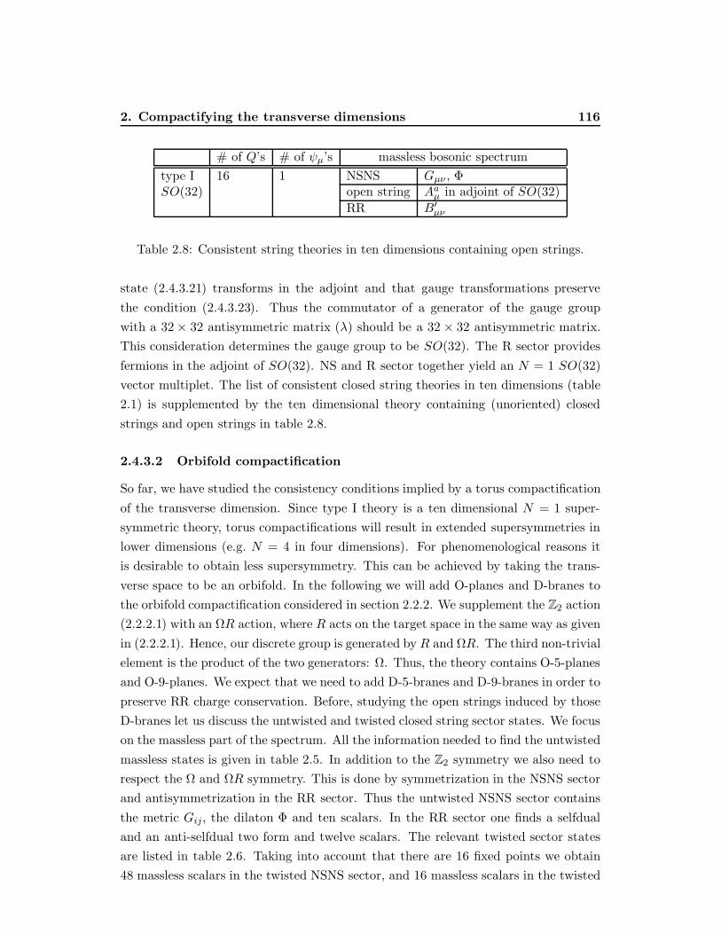
2. Compactifying the transverse dimensions 116
# of Q’s # of ψµ’s massless bosonic spectrum
type I 16 1 NSNS Gµν , ΦSO(32) open string Aaµ in adjoint of SO(32)
RR B′µν
Table 2.8: Consistent string theories in ten dimensions containing open strings.
state (2.4.3.21) transforms in the adjoint and that gauge transformations preserve
the condition (2.4.3.23). Thus the commutator of a generator of the gauge group
with a 32× 32 antisymmetric matrix (λ) should be a 32 × 32 antisymmetric matrix.
This consideration determines the gauge group to be SO(32). The R sector provides
fermions in the adjoint of SO(32). NS and R sector together yield an N = 1 SO(32)
vector multiplet. The list of consistent closed string theories in ten dimensions (table
2.1) is supplemented by the ten dimensional theory containing (unoriented) closed
strings and open strings in table 2.8.
2.4.3.2 Orbifold compactification
So far, we have studied the consistency conditions implied by a torus compactification
of the transverse dimension. Since type I theory is a ten dimensional N = 1 super-
symmetric theory, torus compactifications will result in extended supersymmetries in
lower dimensions (e.g. N = 4 in four dimensions). For phenomenological reasons it
is desirable to obtain less supersymmetry. This can be achieved by taking the trans-
verse space to be an orbifold. In the following we will add O-planes and D-branes to
the orbifold compactification considered in section 2.2.2. We supplement the Z2 action
(2.2.2.1) with an ΩR action, where R acts on the target space in the same way as given
in (2.2.2.1). Hence, our discrete group is generated by R and ΩR. The third non-trivial
element is the product of the two generators: Ω. Thus, the theory contains O-5-planes
and O-9-planes. We expect that we need to add D-5-branes and D-9-branes in order to
preserve RR charge conservation. Before, studying the open strings induced by those
D-branes let us discuss the untwisted and twisted closed string sector states. We focus
on the massless part of the spectrum. All the information needed to find the untwisted
massless states is given in table 2.5. In addition to the Z2 symmetry we also need to
respect the Ω and ΩR symmetry. This is done by symmetrization in the NSNS sector
and antisymmetrization in the RR sector. Thus the untwisted NSNS sector contains
the metric Gij , the dilaton Φ and ten scalars. In the RR sector one finds a selfdual
and an anti-selfdual two form and twelve scalars. The relevant twisted sector states
are listed in table 2.6. Taking into account that there are 16 fixed points we obtain
48 massless scalars in the twisted NSNS sector, and 16 massless scalars in the twisted

2. Compactifying the transverse dimensions 117
RR sector. Adding the fermions in the Ω and ΩR invariant combinations of NSR
and RNS sector states, one obtains finally a d = 6, N = 1 supergravity multiplet, one
tensor multiplet and 20 hypermultiplets. (We should emphasize again that the present
review is not self contained as far as the supergravity representations are concerned.
The reader may view the arrangement of the massless states into multiplets as some
additional information which is not really employed in the forthcoming discussions.
In order to obtain a nice overview about supermultiplets in various dimensions we
recommend[399].)
As already mentioned, we need to add D-5- and D-9-branes in order to cancel the
O-plane RR charges. Thus the Chan-Paton matrix is built out of the following blocks:
λ(99) corresponding to strings starting and ending on D-9-branes, λ(55) corresponding
to strings starting and ending on D-5-branes, λ(59) and λ(95) corresponding to open
strings with ND boundary conditions in the compact dimensions. The action of Ω
and ΩR on the Chan-Paton labels is as described in (2.4.3.2). The γΩ and γΩR posses
also a block structure distinguishing between the action on a string end at a D-5- or
D-9-brane, e.g. γ(9)Ω represents the Ω action on a Chan-Paton label corresponding to
an open string end on a D-9-brane. Finally, we specify the representation of the Z2
element R (2.2.2.1) as follows
R : |ψ, ij〉 → (γR)ii′∣∣R (ψ) , i′j ′
⟩ (γ−1R
)j′j . (2.4.3.24)
Also, the γR can be split into two blocks: γ(9)R and γ
(5)R . The requirement that perform-
ing twice the same Z2 action should leave the state invariant leads to the conditions
that every gamma-block containing an Ω in the subscript must be either symmetric
or anti-symmetric, whereas the gamma-blocks without an Ω in the subscript must
square to the identity58. At this point, we need to discuss a subtlety of the five-nine
sector, i.e. strings with ND boundary conditions along the compact dimensions. In
that sector the Fock space state (without the Chan-Paton label) has an Ω2 and an
(ΩR)2 eigenvalue of minus one. Unfortunately, we did not develop the techniques
needed to show this, in this review. An argument employing an isomorphism between
the algebra of vertex operators and Fock space states can be found in[204]. Since Ω2
and (ΩR)2 should leave states invariant, this minus sign needs to be canceled by an
appropriate action on the Chan-Paton labels. For example a symmetric γ(9)Ω implies
an anti-symmetric γ(5)Ω , and a symmetric γ
(5)ΩR implies an anti-symmetric γ
(9)ΩR.
Let us now study the amplitudes in the loop channel. For strings starting and end-
ing on D-9-branes there is a tower of Kaluza-Klein momentum modes but no winding
modes. The D-9-branes are space filling and thus must lie on top of each other. Open
58We fix a possible phase to one.

2. Compactifying the transverse dimensions 118
strings with both ends on a D-5-brane can have winding modes and can be separated
in the compact directions. (In our previous computation we did not consider this sep-
aration, because it is not relevant in the tree channel infrared limit. In order to see
explicitly that the dependence on the distance among D-5-branes drops out, we will
take it into account, here. We call the component of the position of the ith brane cai .)
Further, all amplitudes obtain an additional insertion
1 +R
2, (2.4.3.25)
ensuring that we trace only over states which are invariant under the orbifold group.
For terms containing an R insertion the D-5-brane must be located at R fixed points,
since otherwise the states in the (55) sector are not eigenstates under R. For the same
reason the winding or Kaluza-Klein momentum modes have to vanish in the presence
of an R insertion. Further, there will be additional signs for oscillators pointing into
a compact dimension. This modifies the oscillator contribution to the trace in a
straightforward way. (We leave the details as an exercise.) Taking into account all
these effects and the discussion in section 2.3.2 one finds for the annulus amplitude A
A = −V6
4
∫dt
t4(8π2α′
)−3
f
84
(e−πt
)
f81 (e−πt)
(
trγ(9)1
)2( ∞∑
n=−∞e−
2πtn2
ρ
)4
+∑
i,j∈5
(γ
(5)1
)ii
(γ
(5)1
)jj
9∏
a=6
∞∑
w=−∞e−t
(2πw√ρα′+cai −c
aj )
2
2πα′
−2f4
2
(e−πt
)f4
4
(e−πt
)
f41 (e−πt) f4
3 (e−πt)
(16∑
I=1
trγ(5)R,I
)(trγ
(9)R
)
+4f4
3
(e−πt
)f4
4
(e−πt
)
f41 (e−πt) f4
2 (e−πt)
(trγ
(9)R
)2+
16∑
I=1
(tr γ
(5)R,I
)2]
, (2.4.3.26)
where we have formally assigned a gamma with subscript 1 to the action of the identity
element of the orbifold group on the Chan-Paton labels. The sum over i, j ∈ 5 means
that we sum over all Chan-Paton labels belonging to an open string end on a D-5-brane.
The index I = 1, . . . , 16 labels the fixed 5-planes, and a corresponding subscript at a
γ(5) indicates that the D-5-brane is located on the Ith fixed plane.
Next, we want to compute the Klein bottle amplitude K. It contains the insertions
Ω and ΩR. In principle, we have to take the trace over untwisted and twisted sector
states (with the (−)F insertion). Because half of the RR sector states have the opposite
(−)F eigenvalue than the other half, RR sector states do not contribute to the trace
with a (−)F insertion. The same applies to RR and NSNS twisted sector states.
Eigenstates of Ω have zero winding numbers whereas for eigenstates of ΩR the Kaluza-
2. Compactifying the transverse dimensions 119
Klein momenta are zero. With this ingredients we find
K = −8V6
4
∫dt
t4(8π2α′
)−3
f84
(e−2πt
)
f81 (e−2πt)
( ∞∑
n=−∞e−πtn2
ρ
)4
+
( ∞∑
w=−∞e−πtρw
2
)4 . (2.4.3.27)
Finally, for the Mobius strip amplitude M we need to trace over R sector states
with an Ω + ΩR insertion. Eigenstates correspond to open strings starting and ending
on the same brane. According to our earlier assignments, the ΩR eigenvalue of the R
vacuum corresponding to a string ending on a D-5-brane is minus one, and so is the
Ω eigenvalue of the R vacuum corresponding to a string ending on D-9-branes. To
determine the remaining eigenvalues one has to act with R on the Ramond vacuum.
R can be viewed as a 180 rotation and the R vacua as target space spinors. Hence,
half of the Ramond vacua have R eigenvalue minus one and the other half plus one.
For this reason, only D-9-branes contribute to the term with the Ω insertion whereas
only D-5-branes give a non-vanishing result for the trace containing an ΩR insertion.
The result for the Mobius strip is
M =V6
4
∫dt
t4(8π2α′
)−3 f82
(e−2πt
)f8
4
(e−2πt
)
f81 (e−2πt) f8
3 (e−2πt)tr
((γ
(9)Ω
)−1 (γ
(9)Ω
)T)( ∞∑
n=−∞e− 2πtn2
ρ
)4
+tr
((γ
(5)ΩR
)−1 (γ
(5)ΩR
)T)( ∞∑
w=−∞e−2πtρw2
)4 . (2.4.3.28)
With the next steps necessary to compute the total RR charge of the system we
are familiar by now. We replace t = 12l in the annulus, t = 1
4l in the Klein bottle
and t = 18l in the Mobius strip. In order to be able to read off the infrared (large l)
asymptotics we use formulæ (2.3.2.22) and (2.4.3.12). The final result is
A+ K+M −→ −V6
4
∫
l→∞dl(4π2α′
)3[ρ2
(trγ
(9)1
)2− 32tr
((γ
(9)Ω
)−1(γΩ)T
)+ 322
+1
ρ2
(trγ
(5)1
)2− 32tr
((γ
(5)ΩR
)−1(γΩ)T
)+ 322
+1
4
16∑
I=1
(trγ
(9)R + 4trγ
(5)R,I
)2]. (2.4.3.29)
2. Compactifying the transverse dimensions 120
The setup respects RR charge conservation if (2.4.3.29) vanishes. Thus, we need 32
D-9-branes and 32 D-5-branes. (A gamma representing the identity is of course the
identity matrix.) Further, we take
γ(5)ΩR =
(γ
(5)ΩR
)T, γ
(9)Ω =
(γ
(9)Ω
)T. (2.4.3.30)
Our previous discussion of the (59) sector implies
γ(5)Ω = −
(γ
(5)Ω
)T, γ
(9)ΩR = −
(γ
(9)ΩR
)T. (2.4.3.31)
The remaining representation matrices can be found by imposing that the gammas
should form a projective59 representation of the orientifold group (Z2 × Z2). We
simply choose
γ(5)R = γ
(5)ΩRγ
(5)Ω (2.4.3.32)
γ(9)R = γ
(9)ΩRγ
(9)Ω . (2.4.3.33)
By fixing a basis in the Chan-Paton labels we obtain
γ(5)ΩR = γ
(9)Ω = I, (2.4.3.34)
where the rank of the identity matrix is 32. The antisymmetric form is
γ(5)Ω = γ
(9)ΩR =
(0 iI
−iI 0
), (2.4.3.35)
with I being a 16× 16 identity matrix, here. Note that our choice is consistent with
the requirement that γ(·)R squares to the identity. So far, we did not take into account
that the last term in (2.4.3.29) has to vanish. With γ(·)R being traceless this is ensured.
We have now all the ingredients needed to determine the open string spectrum. Let
us first study strings starting and ending on the D-9-branes, or in short the (99) sector.
We keep states which are invariant under each element of the orientifold group. (The
D-9-branes are fixed under each element of the orientifold group.) In the NS sector
we find massless vectors with the Chan-Paton matrix
λ(99)vector =
(A S
−S A
), (2.4.3.36)
where A denotes a real antisymmetric and otherwise arbitrary 16× 16 matrix and S
stands for a real 16× 16 symmetric matrix. For the scalars in the NS sector one finds
λ(99)scalars =
(A1 A2
A2 −A1
), (2.4.3.37)
59“Projective” means up to phase factors, which drop out since the gamma acts in combinationwith its inverse on the Chan-Paton label.

2. Compactifying the transverse dimensions 121
where the Ai are 16 × 16 antisymmetric matrices. Let us ignore the D-5-branes for
a moment and determine the gauge group and its action on the scalars in the (99)
sector. Since the vectors are in the adjoint of the gauge group, the gauge group should
be 162 dimensional. U (16) is a good candidate. Further, we know that the vector
should transform in the adjoint under global gauge transformations under which it
should not change the form specified by (2.4.3.36). Thus, we define an element of the
gauge group as
g(9) = exp
(Ag Sg
−Sg Ag
), (2.4.3.38)
where Sg (Ag) are real anti-(symmetric) matrices with infinitesimal entries. A gauge
transformation acts on the Chan-Paton matrix as
λ(99)→ g(9)λ(99)(g(9))−1
=
[(Ag Sg
−Sg Ag
), λ
]. (2.4.3.39)
We observe that the vectors transform in the adjoint and the form of the Chan-Paton
matrix is preserved. Note also that g(9) is unitary and has 162 parameters. It is a
U (16) element. The U (1) subgroup corresponds to Ag = 0 and Sg proportional to the
identity. From our assignment that the Chan-Paton matrix transforms in the adjoint
of U (16) it is also clear that the Chan-Paton label i and j transform in the 16 and
16 of U (16) Thus, the scalars can be decomposed into the antisymmetric 120 + 120.
One may also explicitly check that the form of the Chan-Paton matrix for the scalars
is not altered by a gauge transformation. We leave the discussion of the fermions in
the R sector as an exercise. The result is that that half of them carry the Chan-Paton
matrix (2.4.3.36) and the other half the matrix (2.4.3.39). Altogether the (99) sector
provides a vector multiplet in the adjoint of U (16) and a hypermultiplet in the 120
+ 120.
Now, we include the D-5-branes. Here, we have to distinguish between the case
that a D-5-brane is situated at a fixed plane or not. In the first case the (55) strings
have to respect the ΩR and R symmetry, whereas in the second case these orientifold
group elements just fix the fields on the image brane. Suppose we have 2mI D-5-branes
at the Ith fixed plane. (The number of the D-5-branes per fixed plane must be even,
since otherwise they cannot form a representation of the orientifold group.) The NS
sector leads again to a massless vector and massless scalars with almost the same Chan-
Paton matrices as in the (99) sector ((2.4.3.36) and (2.4.3.39)). The only difference is
that the antisymmetric and symmetric matrices are now mI ×mI instead of 16× 16.
Hence, we obtain a vector multiplet in the adjoint of U (mI) and a hypermultiplet in
the mI
2 (mI-1) + mI
2 (mI-1).

2. Compactifying the transverse dimensions 122
Let 2nj D-5-branes be situated away from the fixed plane (but on top of each other).
For the (55) sector belonging to those D-5-branes we impose invariance under Ω, only.
The solution for γ(5)Ω is given in (2.4.3.35). Together with the minus eigenvalue on the
massless NS sector Fock space state, this leads to the result that the vector in the (55)
sector is an element of the USp (2nj) Lie algebra in the adjoint representation. Taking
into account (part of) the R sector this is promoted to a USp (2nj) vector multiplet.
The scalars together with the remaining R sector states form a hypermultiplet in the
antisymmetric nj (2nj-1) representation.
It remains to study the (95) sector. (Here, one has to take into account that
along the compact directions NS sector fermions are integer modded whereas R sector
fermions are half integer modded. This is quite similar to the twisted sector closed
string. In particular, the (95) NS sector ground state is already massless. Hence,
the NS sector does not give rise to massless vectors. We do not impose Ω or ΩR
invariance on (95) strings since they are mapped onto (59) strings by the worldsheet
parity inversion. If the considered D-5-branes are situated at one of the fixed planes
we impose R invariance. In this case, one finds in the NS sector two scalars with the
Chan-Paton matrix
λ(95) =
(X1 X2
−X2 X1
), (2.4.3.40)
where the Xi are general mi × 16 matrices. Together with the R sector this leads to
a hypermultiplet in the (16 , mI) of U (16)× U (mI), (the hypermultiplet is neutral
under the gauge group living on D-5-branes not situated at the Ith fixed plane). For
D-5-branes which are not a fixed plane the (95) sector provides a hypermultiplet in
the (16, 2nJ) of U (16)× USp (2nj).
Altogether we find the gauge group is
U (16)×16∏
I=1
U (mI)×∏
J
USp (2nj) , (2.4.3.41)
where j labels the D-5-brane packs away from fixed planes. In addition the total
number of D-5-branes has to be 32 (images are counted), i.e.
16∑
I=1
2mI + 2∑
j
2nj = 32. (2.4.3.42)
There are hypermultiplets in the representation
2 (120 , 1, 1) +16∑
I=1
2
(1,
1
2mI (mI-1) , 1
)
I
+ (16,mI , 1)I
+∑
j
(1, 1,nj (2nj-1) -1)j + (1, 1, 1) + (16, 1, 2nj)j
, (2.4.3.43)

2. Compactifying the transverse dimensions 123
where we have split the anti-symmetric representation of USp (2nj) into its irreducible
parts and an index I , j refers to the gauge group on the D-5-brane pack at a fixed plane
and off a fixed plane, respectively. It can be checked that the effective six dimensional
theory is free of anomalies. The models belonging to different distributions of the
D-5-branes on and off fixed planes can be continuously transformed into each other.
In the field theory description this corresponds to the Higgs mechanism.
We have seen that adding to the orbifold compactification of section 2.2 O-planes
and D-branes gives a very interesting picture. Apart from the closed string twisted
sector states located at the orbifold fixed planes we obtain various fields from open
strings ending on D-branes. These D-branes can be moved within the compact direc-
tions while keeping the geometry fixed. The techniques described in this section can be
also applied to phenomenologically more interesting setups leading to four dimensional
theories. A description of such models is beyond the scope of the present review.
Chapter 3
Non-Perturbative description of
branes
3.1 Preliminaries
In the previous sections we gave a perturbative description of various extended ob-
jects: the fundamental string, orbifold planes, D-branes and Orientifold planes. The
string plays an outstanding role in the sense that field theories on the worldvolumes
of the other extended objects are effective string theories. The quantization of the
fundamental string is performed in a trivial target space (i.e. the target space metric
is the Minkowski metric and all other string excitations are constant or zero). Further,
the worldsheet topology is specified to the spherical (for closed strings) or disc (for
open strings) topology (after Wick rotating to Euclidean worldsheet signature). Our
treatment leads to a perturbative expansion in the genus of the worldsheet (see section
2.1.4). The perturbative expansion is governed by the string coupling
gs = e〈Φ〉, (3.1.0.1)
which needs to be small. Perturbative closed string theory has an effective field theory
description which contains supergravity. How does one obtain insight into regions
where gs is large? Clearly, the perturbation theory breaks down in this case, and
indeed this region is rather difficult to study. There are, however, a few results one
can obtain also for strong couplings. Let us recall how non perturbative effects in Yang-
Mills theory can be studied. Apart from the trivial vacuum, (Euclidean) Yang-Mills
theory contains several other stable vacua, viz. the instantons. Studying fluctuations
around an instanton vacuum, one finds an additional weight factor in the path integral
which comes from the background value of the action and is of the form
e− ng2 ,
124

3. Universal Branes 125
where n is the instanton number and g is the Yang-Mills gauge coupling. As long as g is
small, the fluctuations around an instanton vacuum are heavily suppressed. However,
as soon as g becomes large, the suppression factor becomes large. Thus, knowing about
the instanton solutions in Yang-Mills theory gives a handle on non perturbative effects.
But how can one know, that one does not have to include strong coupling effects into
the theory before deriving the instanton solutions? The answer is that instantons are
stable, they are characterized by a topological number which cannot be changed in
a continuous way when taking g from small to large. Therefore, instantons can give
information about strongly coupled Yang-Mills theory even though they are found as
solutions to the perturbative formulation of Yang-Mills theories. States (vacua) with
such a feature are called BPS states.12
Therefore, our aim will be to find BPS states in string theory. In the low energy
limit, the various superstring theories are described by supergravities. Insights into
non-perturbative effects in string theory can be gained by finding the BPS states of
perturbative string theory. As a guiding principle, we will look for solutions to the
effective equations of motion that preserve part of the supersymmetry (i.e. are invariant
under a subset of the supersymmetry transformations). Roughly speaking, it is then
the number of preserved supersymmetries which cannot be changed continuously when
taking the string coupling from weak to strong. We will see that such solutions can
be viewed as branes. The number of branes takes the role of the instanton number
in the Yang-Mills example discussed above. We will be very brief in our analysis and
essentially only summarize some of the important results. The classical review on
branes as supergravity solutions is[152] and we will give more references in the end of
this review.
3.2 Universal Branes
From section 2.1.4 we recall that all the closed superstring theory effective actions
contain a piece
Suniv =1
2κ2
∫d10x√−Ge−2Φ
(R+ 4 (∂Φ)2 − 1
12H2
). (3.2.0.1)
In the present section we will truncate all closed string effective field theories to (the
supersymmetric extension of) (3.2.0.1). This is consistent because we will restrict on
backgrounds where the discarded part of the action vanishes and the corresponding
equations of motion are satisfied trivially. By adding appropriate terms including
1There are also stable non BPS states (for reviews see e.g. [424, 319, 195]). We will not discussthese.
2BPS stands for the names Bogomolny, Prasad and Sommerfield, and refers to the papers[76, 379].
3. Universal Branes 126
fermions (2.1.4.5) can be promoted to an N = 1 supersymmetric theory. (For type II
theories this is a sub-symmetry of the N = 2 supersymmetry.) The supersymmetric
extension is usually given in the Einstein frame. The action (3.2.0.1) is written in the
string frame were the string tension is a constant and independent of the dilaton. The
Einstein frame is obtained by the metric redefinition
gµν = e−Φ2 Gµν , (3.2.0.2)
where Gµν is the string frame metric and gµν is the Einstein frame metric. The action
(3.2.0.1) takes the form
SE,univ =1
2κ2
∫d10x√−g
(R− 1
2(∂Φ)2 − 1
12e−ΦH2
). (3.2.0.3)
We observe that (3.2.0.3) starts with the familiar Einstein Hilbert term (therefore the
name “Einstein frame”). Further, the kinetic term of the dilaton has the “correct”
sign now, and the coupling of the B field is Φ dependent. In the supersymmetric
extension, a gravitino and a dilatino are added. We do not give the supersymmetric
action explicitly. For us, it will suffice to know the supersymmetry transformations of
the gravitino and the dilatino. These are
δψµ = Dµε+1
96e−
Φ2(Γµ
νρκ − 9δνµΓρκ)Hνρκε, (3.2.0.4)
δλ = − 1
2√
2Γµ∂µΦε+
1
24√
2e−
Φ2 ΓµνρHµνρε, (3.2.0.5)
where ψµ denotes the gravitino and λ the dilatino. The Gamma matrices with curved
indices are obtained from ordinary Gamma matrices (16× 16 matrices satisfying the
usual Clifford algebra in ten dimensional Minkowski space) by transforming the flat
index with a vielbein to a curved one. A Gamma with multiple indices denotes the
anti-symmetrized product of Gamma matrices. The spinor ε is the supersymmetry
transformation parameter.
Sometimes it is useful to formulate the theory in a slightly different way. To
this end, one adds to the action (3.2.0.3) a Lagrange multiplier term providing the
constraint of a fulfilled Bianchi identity. Calling the Lagrange multipliers Aµ1 ...µ6 ,
such a term looks like∫d10x εµ1 ...µ10Aµ1 ...µ6∂µ7Hµ8µ9µ10 . (3.2.0.6)
The Aµ1 ...µ6 equation of motion yields the Bianchi identity of the B field strength
Hµνρ. However, one can alternatively solve the B field equation of motion with the
result
Hµνρ ∼ eΦεµνρµ1 ...µ7Kµ1...µ7 , (3.2.0.7)

3. The fundamental string 127
with
Kµ1...µ7 = ∂[µ1Aµ2 ...µ7 ]. (3.2.0.8)
This means that we can trade the antisymmetric tensor B for a six form potential
A. Choosing an appropriate normalization for the Lagrange multiplier terms (3.2.0.6),
the effective action (3.2.0.3) in terms of the six form potential A reads
SE,univ =1
2κ2
∫d10x√−g
(R− 1
2(∂Φ)2 − 1
2 · 7!eΦK2
). (3.2.0.9)
Also in this form the action can be supersymmetrized. In terms of the six form
potential A the gravitino and dilatino supersymmetry transformations read
δψµ = Dµε+1
2 · 8!e
Φ2(3Γµ
ν1 ...ν7 − 7δν1µ Γν2 ...ν7
)Kν1 ...ν7ε, (3.2.0.10)
δλ = − 1
2√
2Γµ∂µΦε − 1
2 · 2√
2 · 7!e
Φ2 Γµ1 ...µ7Kµ1...µ7ε. (3.2.0.11)
In the following two subsections, we will present two solutions preserving half of
the supersymmetry.
3.2.1 The fundamental string
The solutions we are going to discuss in the present and subsequent sections are gen-
eralizations of extreme Reissner–Nordstrom black holes. Reissner–Nordstrom black
holes are solutions of Einstein–Hilbert gravity coupled to an electro magnetic field.
They carry mass and electric or magnetic charge. Extreme Reissner–Nordstrom black
holes satisfy a certain relation between the charge and the mass. (In our case such
a relation will be dictated by the requirement of partially preserved supersymmetry.)
Replacing the electro magnetic field strength F by its dual ?F interchanges electric
with magnetic charge. (For a more detailed discussion of Reissner–Nordstrom black
holes see e.g.[442].)
The action (3.2.0.3) bears some analogy to four dimensional Einstein gravity cou-
pled to an electro magnetic field. The difference is that the theory is ten dimensional
instead of four dimensional and the electro magnetic field strength is replaced by the
three form H . In addition, there is the scalar Φ. Since the gauge potential is now a
two form which naturally couples to the worldvolume of a string, we look for “extreme
Reissner–Nordstrom black strings” instead of black holes. The corresponding ansatz
for the metric is
ds2 = e2Aηijdxidxj + e2Bδabdy
adyb, (3.2.1.1)

3. The fundamental string 128
with i, j = 0, 1 and a, b = 2, . . . , 9. Further, A and B are functions of
r =√δabyayb, (3.2.1.2)
only. Here, we have taken the second step before the first one in the sense that
first we should have thought about what kind of isometries we would like to obtain
and only afterwards we should have written down a general ansatz respecting the
isometries. Therefore, let us perform the first step now and discuss the isometries of
the ansatz. Clearly, there is an SO (1, 1) isometry acting on the xi. This means, that
up to Lorentz boosts, xi spans the worldvolume of a straight static string. There is no
further dependence on xi in the ansatz because we do not wish to distinguish a point
on the worldvolume of the string. The other isometry acts as an SO (8) on the ya.
This is the natural extension of the SO (3) isometry associated with non-rotating four
dimensional black holes. It is SO (8) now because the space transverse to the string is
eight dimensional (whereas in 4d black holes the space transverse to the hole is three
dimensional). The r dependence respects the SO (8) isometry. Distinguishing between
different values of r means specifying the position of the string, i.e. r measures the
radial distance from the string.
In order not to spoil the above symmetries, we choose for the remaining fields the
ansatz
B01 = −eC , Φ = Φ (r) , (3.2.1.3)
where C is also a function of r only. All other components of B are zero. Viewed as a
two form, B is proportional to the invariant volume form of the string worldvolume.
The factor eC may depend on r.
The ansatz for the target space spinors is that they all vanish. As mentioned earlier
we are interested in situations where the solution preserves part of the supersymmetry
because this ensures that we can continuously take the string coupling from weak to
strong. In particular, the unbroken supersymmetry is parameterized by spinors ε for
which the gravitino and dilatino values of zero do not change under supersymmetry
transformations, i.e. those ε for which the rhs of (3.2.0.4) and (3.2.0.5) vanish. In order
to find such solutions for our ansatz it is convenient to represent the ten dimensional
Gamma matrices A,B = 0, . . . , 9,
ΓA,ΓB = 2ηAB (3.2.1.4)
as a tensor product of 2×2 matrices γi in 1+1 and 8×8 matrices Σa in 8 dimensions3
ΓA = (γi ⊗ I, γ3 ⊗ Σa) , (3.2.1.5)
3The corresponding algebras are γi, γj = 2ηij and Σa,Σb = 2δab.
3. The fundamental string 129
where I is the 8× 8 identity matrix and
γ3 = γ0γ1 (3.2.1.6)
squares to the 2 × 2 identity matrix. Further, we have to take into account that the
ten dimensional N = 1 supersymmetry parameter ε is subject to the constraint
Γ11ε = ε. (3.2.1.7)
Under certain conditions to be specified below the variations of the gravitino and the
dilatino vanish for
ε = e3Φ8 ε0 ⊗ η0, (3.2.1.8)
where ε0 and η0 are SO (1, 1) and SO (8) constant spinors, respectively, which satisfy
the lower dimensional chirality conditions
(1− γ3) ε0 = 0 ,
(1−
9∏
a=2
Σa
)η0 = 0. (3.2.1.9)
This breaks the supersymmetry to half the amount of the perturbative (trivial) vac-
uum. (The condition (3.2.1.7) could be also satisfied by choosing simultaneously the
opposite chiralities in the two equations (3.2.1.9).)
We already mentioned that only under certain conditions we can find unbroken
supersymmetries at all. Requiring that asymptotically (r→∞) we obtain the pertur-
bative vacuum, these conditions read
A =3
4(Φ− Φ0) , (3.2.1.10)
B = −1
4(Φ− Φ0) , (3.2.1.11)
C = 2Φ− 3
2Φ0 (3.2.1.12)
where Φ0 is the asymptotic value of Φ. Hence supersymmetry leaves only one function
out of our ansatz undetermined. This function can be taken to be the dilaton whose
equation of motion boils down to
δab∂a∂be−2Φ(r) = 0, (3.2.1.13)
i.e. the “flat” Laplacian of the transverse space (spanned by the ya) acting on e−2Φ
has to vanish. As in the case of four dimensional black holes, we solve this equation
everywhere but at the origin r = 0, where there are additional contributions due to
a source string. (We do not add the source string explicitly here, but will infer its
3. The fundamental string 130
properties (tension and charge) in an indirect way below. For the explicit inclusion of
the source term see e.g.[152].) The solution to (3.2.1.13) reads
e−2Φ = e−2Φ0
(1 +
k
r6
), (3.2.1.14)
where k is an integration constant which will be related to the string tension below.
Plugging this back into (3.2.1.10) – (3.2.1.12) and in the ansatz gives the final solution.
Next, we would like to deduce the tension of the string source from our solution.
This is done by studying the Newtonian limit of general relativity. In particular, by
comparing the Einstein equation with the geodesic equation of a point particle (which
has constant mass in the Einstein frame) one finds that the Newton potential of the
string-source is encoded in the subleading term in a large r expansion of g00. Therefore,
we first observe that for large r
g00 = −1 +3k
4r6+ . . . . (3.2.1.15)
The relation between g00 and the Newton potential of a string is explicitly such that4
1
r7∂r(r7∂rg00
)= −3
2κ2TE
δ (r)
Ω7r7(3.2.1.16)
holds, with the understanding that terms denoted by . . . in (3.2.1.15) are neglected.
The string tension is denoted by TE. Further, the unit volume of a seven–sphere Ω7
enters the expression. Hence, we obtain
TE =3k
κ2Ω7. (3.2.1.17)
We put the index E at the tension in order to indicate that it is measured in the Ein-
stein frame. What we are actually interested in, is the tension in the string frame. This
is readily obtained by noticing that transforming back to the string frame (asymptot-
ically) implies
κ2 → e2Φ0κ2 , Ω7 → e7Φ0
2 Ω7. (3.2.1.18)
Thus in the string frame the tension is5
T =3k
κ2e
3Φ02 Ω7. (3.2.1.19)
4Equation (3.2.1.16) has the same form as the equation satisfied by the Newton potential. Thenumerical factor of 3
2= 7−p
4on the rhs of (3.2.1.16) is a matter of convention, which fixes the relation
between κ, the speed of light (c = 1), and Newton’s constant (see e.g.[432]). We choose our conventionin agreement with[152], where explicit source terms (containing the tension) are added.
5On dimensional grounds, one would expect a different scaling of T . In order to obtain this, onehas to take into account that k is a dimensionful quantity. In (3.2.1.19) k is given Einstein frameunits.

3. The NS five brane 131
Recalling that our “elementary particle” is a string of tension 12πα′ and requiring that
any string like object must consist out of an integer number N of elementary strings
we finally determine the integration constant k to be6
k = Nκ2
6πα′Ω7e−
3Φ02 . (3.2.1.20)
It remains to compute the U (1) charge carried by the vacuum. This is basically
done by integrating the B equation of motion over the transverse space. The result is
µ =1√2κ
∫
S7
e−Φ ? H, (3.2.1.21)
where the integration is over an asymptotic seven-sphere enclosing the string source.
The U (1) charge is denoted by µ. Expressing the result in terms of the string tension
one obtains
µ =√
2κN
2πα′. (3.2.1.22)
This equality is related to partially unbroken supersymmetry. If the configuration
was not stable the tension of the bound state would be larger than the sum of the
elementary tensions. Hence, the rhs of (3.2.1.22) is larger for general (non BPS) states.
The BPS state saturates a general inequality. Since the BPS state is stable, there can
be no state with less tension and the same charge since otherwise the BPS state would
decay into such a state. The lower bound on the tension set by the BPS state is called
the Bogomolnyi bound.
3.2.2 The NS five brane
In this subsection we repeat the analysis of the previous section, however, with the
action (3.2.0.9) instead of (3.2.0.3). Thus, we will obtain the magnetic dual of the
previously discussed string solution. This is called the NS five brane. Its properties
(tension, charge) will be fixed in terms of the string properties via the Dirac quanti-
zation condition. (For generalizations of the Dirac quantization condition to extended
objects see[353, 438].) As the derivation of the NS five brane solution goes along the
same lines as the one given in the previous subsection, we will be even more sketchy
here. Instead of the two form potential, we have now the six form potential A. Since
an object which extends along five spatial dimensions naturally couples to a six form
potential, we choose the following ansatz for the metric
ds2 = e2Aηijdxidxj + e2Bδabdy
adyb, (3.2.2.1)
6Here we use the fact that for a superposition of BPS states there is no binding energy, i.e. thetotal tension is obtained by simply summing the tensions of the individual BPS states.

3. The NS five brane 132
where now i, j = 0, . . . , 5 and a, b = 6, . . . , 9. The five brane worldvolume extends
along the xi directions and the functions A and B are allowed to depend on the radial
distance from the five brane r with
r =√δabyayb. (3.2.2.2)
The ansatz for the six form potential is
A012345 = −eC , (3.2.2.3)
where C is a function of r. The components of A which cannot be obtained by
permuting the indices in (3.2.2.3) are zero. The final input is that also the dilaton
depends only on r,
Φ = Φ (r) . (3.2.2.4)
All fermionic fields are again set to zero. There is an unbroken supersymmetry if
we can find a spinor such that the gravitino and dilatino transformations (3.2.0.10)
and (3.2.0.11) vanish. It turns out that half of the supersymmetry is preserved if the
following relations hold
A = −1
4(Φ− Φ0) , (3.2.2.5)
B =3
4(Φ− Φ0) , (3.2.2.6)
C = −2Φ +3
2Φ0, (3.2.2.7)
where Φ0 denotes again the asymptotic r → ∞ value of the dilaton. (In addition
to partially unbroken supersymmetry we have once again imposed that for large r
the vacuum should approach the perturbative vacuum.) Under these conditions the
equations of motion boil down to
δab∂a∂be2Φ = 0. (3.2.2.8)
We solve this equation everywhere but at r = 0 where we allow for additional contri-
butions due to source terms. One finds
e2(Φ−Φ0) = 1 +k
r2. (3.2.2.9)
The integration constant k can be fixed by exploiting the Dirac quantization condition.
To this end we compute the charge carried by the vacuum
µ =1√2κ
∫
S3
eΦ ? K =
√2Ω3k
κe
Φ02 , (3.2.2.10)
3. The NS five brane 133
where the integral is over an asymptotic three–sphere surrounding the five brane and
Ω3 denotes the volume of a unit three–sphere. Now, the Dirac quantization condition
reads
µµ = 2πNN, (3.2.2.11)
where µ is the charge of N elementary strings (3.2.1.22). The number of five branes
(number of magnetic charges) is N . This fixes the integration constant,
k =πN
TSΩ3e−
Φ02 , (3.2.2.12)
where TS is the elementary string tension (TS = 12πα′ in the string frame). By com-
puting the gravitational potential in the Newtonian limit, one finds the tension of the
five brane in the Einstein frame (with TS and κ also in Einstein frame units)
TE =πN
TSκ2e−
Φ02 . (3.2.2.13)
The mass dimension of TE is six. Hence, we obtain
T = e−2Φ02πα′πNκ2
(3.2.2.14)
in the string frame. We observe that the five brane tension behaves as 1/g2s . In the
perturbative region the NS five brane is very heavy whereas it becomes lighter when
the string coupling increases.
The NS five brane is an extended object for which we did not give a perturbative
description. Indeed, such a description is not known. One could try to quantize strings
in the NS five brane background. This is possible only in certain spatial regions.
Firstly, for large r the background becomes flat, and we know how to quantize strings
there. But also in the background at r → 0 (the near horizon limit) one can find a
quantized string theory. In that limit the string frame metric reads
ds2s = ηijdx
idxj + k (d log r)2 + kdΩ23, (3.2.2.15)
and the dilaton is linear in ρ = log r. With dΩ23 we denote the metric of a unit three–
sphere. The NSNS field strength H is a constant times the volume element dΩ3. The
geometry factorises into a 5 + 1 dimensional Minkowski space times the direction on
which the dilaton depends linearly times an S3. Since S3 is an SU (2) group manifold,
string theory can be quantized in such a background. For more details see[97] or the
review[96].

3. Type II branes 134
3.3 Type II branes
Like in the previous sections, we are interested in setups where only a truncated version
of the effective actions (see section 2.1.4 ) is relevant. The bosonic part of the truncated
type II action reads
S =1
2κ2
∫d10x
(e−2Φ
(R+ 4 (∂Φ)2
)− 1
2 (p+ 2)!F 2p+2
), (3.3.0.1)
where Fp+2 denotes the field strength of an RR p+ 1 form potential. For type IIA p is
even whereas it is odd for type IIB theory. For p = 3 the action has to be supplemented
by the constraint that the field strength is selfdual. The (p+2 form) field strengths are
not all independent but related by Hodge duality to the field strength corresponding
to 6 − p (an 8 − p form field strength). We will restrict the discussion to the cases
0 ≤ p < 7. For p = 7 the solution presented in[225] is relevant. The 8-brane appears
as a solution of massive type IIA supergravity[56]. How this is related to string theory
(or rather M-theory) is discussed in the recent paper[236] (see also references therein).
We will consider only a single relevant p at a time. The field redefinition (3.2.0.2)
takes us to the action in the Einstein frame
SE =1
2κ2
∫d10x√−g
(R− 1
2(∂Φ)2 − 1
2 (p+ 2)!e
3−p2
ΦF 2p+2
). (3.3.0.2)
The p-brane ansatz reads
ds2 = e2Aηijdxidxj + e2Bδabdy
adyb, (3.3.0.3)
with i, j = 0, . . . , p and a, b = p+ 1, . . . , 9. A and B are functions of
r =√δabyayb (3.3.0.4)
The dilaton is also taken to be a function of r. Let us first exclude the case p = 3 from
the discussion. For the p+ 1 form gauge field we choose
A0,... ,p = −eC , (3.3.0.5)
where C is a function of r, and all other components of A (which cannot be obtained
by permuting the indices in (3.3.0.5)) are zero. All the other fields (NSNS B-field, the
remaining RR forms, and the fermions) are zero. The BPS condition leaves one out
of the four functions A, B, C and Φ undetermined. Choosing for convenience C to be
the undetermined function, these conditions read
A =7− p
16(C − C0) , (3.3.0.6)
B = −p+ 1
16(C − C0) , (3.3.0.7)
Φ =p− 3
4(C − C0) +
4C0
p− 3, (3.3.0.8)
3. Type II branes 135
where again the boundary condition that for r→∞ the background should be trivial
has been imposed. C0 denotes the asymptotic value of C which is related to the
asymptotic dilaton value
C0 =p− 3
4Φ0. (3.3.0.9)
The equations of motion reduce to
δab∂a∂be−C = 0. (3.3.0.10)
We solve this by
e−C = e−C0 +kpr7−p . (3.3.0.11)
The RR charge of the vacuum is
µp =1√2κ
∫
S8−pe
3−p2
Φ ? Fp+2 =7− p√
2κΩ8−pkp, (3.3.0.12)
where the integration is over an asymptotic (8− p)–sphere surrounding the p brane,
and Ω8−p is the volume of the unit sphere. Now we try whether we can identify the
type II p-branes with the D-branes discussed in section 2.3. This trial is motivated by
the observation that the D-branes considered in section 2.3 are also extended objects
carrying RR charge. In section 2.3 we computed the charge of a single D-brane to be
(see (2.3.2.31) and (2.3.2.29))
µsingle branep =
√2π(4π2α′
) 3−p2 . (3.3.0.13)
Assuming that the vacuum considered in the present section is composed out of an
integer number Np of single D-branes, we identify (TS denotes the frame dependent
tension of a single fundamental string)
kp = Np2κ(4π2/TS
) 3−p2√π
(7− p) Ω8−p, (3.3.0.14)
such that
µp = Npµsingle branep . (3.3.0.15)
A first consistency check is to observe that the Dirac quantization condition
µpµ6−p = 2πNpN6−p (3.3.0.16)
is satisfied. After we have fixed the integration constant kp the tension of the brane
solution is determined. Because the vacuum considered here and the D-branes consid-
ered in section 2.3 are BPS objects the tension is related to the charge and we expect

3. Type II branes 136
that our tension should be in agreement with (2.3.2.29). Let us nevertheless compute
it explicitly. To this end, we write down the asymptotic expansion of g00
g00 = −1 +7− p
8
kpr7−p e
p−34
Φ0 + . . . . (3.3.0.17)
The tension is given via (see also (3.2.1.16))
1
r8−p∂r(r8−p∂rg00
)= −7− p
4κ2Tp,E
δ (r)
Ω8−pr8−p , (3.3.0.18)
where Tp,E denotes the tension in Einstein frame units and it is understood that terms
denoted by dots in (3.3.0.17) are neglected. This yields
Tp,E =7− p2κ2
Ω8−pkpep−3
4Φ0 . (3.3.0.19)
Since Tp,E has mass dimension p + 1, it receives a factor of e−p+1
4Φ under the trans-
formation to the string frame. Taking this and (3.3.0.14) into account, we find for the
string frame tension
Tp = Npe−Φ0κ
√π(4π2α′
) 3−p2
1
κ, (3.3.0.20)
in agreement with (2.3.2.29). Thus, we found that the p-brane vacuum can be viewed as
consisting out of an integer number of “elementary” (or magnetic) D-branes considered
in section 2.3.
So far, we have derived this result only in the case p 6= 3. In the case p = 3, the
condition (3.3.0.8) is changed into
Φ = Φ0 , C0 = 0. (3.3.0.21)
The selfduality condition can be imposed by replacing F5 from our ansatz with F5+?F5,
F5 → F5 + ?F5. (3.3.0.22)
The solution for C is
e−C = 1 +k3
r4. (3.3.0.23)
The “electric” charge is
µ3 =1√2κ
∫
S5
?dA0123 =4√2κ
Ω5k3. (3.3.0.24)
The replacement (3.3.0.22) implies that the solution carries also a magnetic charge
µp = µp. Thus, the Dirac quantization condition yields (N3 is the number of D3-
branes)
k3 = N3
√πκ
2Ω5, (3.3.0.25)
3. Type II branes 137
such that
µ3 =√
2πN3. (3.3.0.26)
For the tension, one obtains in the string frame
T3 = N3e−Φ0
√π
κ. (3.3.0.27)
Thus, also for p = 3 we can consistently assume that the vacuum solution is made out
of an integer number of the D3-branes introduced in section 2.3. We will return to the
solution for p = 3 in section 4.3.
We stop our discussion on the appearance of branes as vacua of the effective actions
at this point. We should, however, mention that there are many more configurations
which can be constructed. For example, one can find vacua where branes lie within
the worldvolume of other higher dimensional branes. Such studies confirm the result
of section 2.3.1.3 that supersymmetry is completely broken unless the number of ND
directions is an integer multiple of four.
A final remark about the BPS vacua of type I theory is in order. Although we
called this section “type II branes”, the discussion applies to type I theory as well. In
the closed string sector of type I theory the NSNS B field is projected out, and thus
there is neither a fundamental string nor an NS five brane vacuum in the effective
type I theory. On the other hand, the RR two form potential survives the projection.
Hence, type I theory possesses the D1 and the D5 brane vacua.

Chapter 4
Applications
In this chapter, we are going to present some applications of the branes discussed so
far. In the following, we will show that branes are a useful tool in supporting duality
conjectures involving an interchange between strong and weak couplings. As a first
example we consider dualities among different string theories. Thereafter, field theory
dualities will be translated into manipulations within certain brane setups. Next, we
want to present the AdS/CFT correspondence – a duality between closed and open
string theory, or in first approximation between gravity and gauge theory. Finally, we
argue that branes allow constructions in which the string scale is about a TeV. Such
setups have the prospect of being discovered in the near future. There are many more
applications of branes in theoretical physics. Some of them we will list in chapter 6
containing suggestions for further reading.
4.1 String dualities
There are many excellent reviews on string dualities and we do not plan to provide an
introduction into this subject here. We just want to summarize how branes are mapped
among each other under duality transformations. We start by drawing the M-theory
star in figure 4.1. The idea behind this picture is that the theories written at the tips
of the “star” are different descriptions of one underlying theory called M-theory. This
underlying theory is not known. It is assumed to possess a moduli space which looks
like figure 4.1. The picture is supported by evidences for the conjecture that all the
other theories appearing in figure 4.1 are related by motions in their moduli spaces.
Let us briefly summarize how these theories are connected. We start at the top of
the star (11D SUGRA) and work our way down to the bottom (type I), first counter
clockwise. Compactifying eleven dimensional supergravity on an interval (S1/Z2)
yields the effective field theory of the heterotic E8 × E8 string. The dilaton is re-
138

4. String dualities 139
M
11 D SUGRA
HeteroticE8 × E8
HeteroticSO (32)
Type I
Type IIB
Type IIA
Figure 4.1: M-theory star
lated to the length of the interval such that the string coupling is small when the
interval is short. The E8 × E8 fields live as twisted sector fields at the ends of the
interval (the orbifold nine planes). If we take the string coupling of the E8 × E8 het-
erotic string to be strong, 11D supergravity on an interval provides the more suitable
description. The connection between the E8 ×E8 and the SO (32) string was already
discussed in section 2.1.5.4. It does not relate strong with weak coupling but small
with large compactification radii in nine dimensions. The heterotic SO (32) string is
connected to type I strings by a strong/weak coupling duality. Now, let us go back
to the top of the star and go down clockwise. Type IIA supergravity can be obtained
by compactifying 11 dimensional supergravity on a circle. The radius of the circle
determines the vev of the dilaton. For small string coupling the circle is small, and
for strong coupling it is large. The connection between type IIA and type IIB strings
is seen by compactifying further down to nine dimensions and inverting the radius, as
argued in section 2.1.5.4. Type I theory is obtained by gauging worldsheet parity of
type IIB strings and adding the D-branes needed to ensure RR-charge conservation
(in a sense these can be viewed as twisted sector states).
Because the branes we have discussed are stable under deformations in the moduli
space, they should be mapped in a one-to-one way onto each other by string dualities.
Since eleven dimensional supergravity did not appear until now in our discussion (it
does not correspond to an effective weakly coupled string theory), we have to list
the relevant BPS branes of 11 dimensional supergravity. 11 dimensional supergravity
contains a three form gauge potential which can be Hodge dualized to a six form gauge
potential. Analogously to the solutions found in the previous chapter, one finds thus
a membrane (2 brane) and a five brane.
4. String dualities 140
Let us now walk once around the star in figure 4.1 in a clockwise direction and follow
the branes along this journey. Upon compactifying one of the eleven dimensions the
momentum into this direction becomes quantized. The off diagonal metric components
containing one 11 label become a Kaluza Klein gauge field – a one form potential, which
can be Hodge dualized (with respect to the non compact directions) to a seven form
potential. The associated BPS states are zero and six branes. These become the D0
and the D6 branes in the type IIA picture. For the branes which exist already in
the uncompactified theory, there are two options within the compactification. The
compact dimension can be transverse or longitudinal. Hence, the membrane will be
either described by a fundamental string or by a D2 brane in weakly coupled type
IIA theory, and the five brane yields the D4 brane and the NS five brane of type IIA
theory.
Compactifying further down to nine dimensions and taking the decompactification
limit after a T-duality transformation, type IIA theory goes over into type IIB theory.
The D-branes gain or lose one spatial direction due to the T-duality, and hence we
obtain all the D-branes of type IIB theory. Type IIB theory possesses a symmetry
which is not depicted in figure 4.1. This is an SL (2,Z) symmetry which we do not
want to discuss in detail. For later use we state that the SL (2,Z) symmetry contains
a transformation called S duality. S duality interchanges strong with weak coupling,
the D1 brane with a fundamental string and the D5 brane with the NS five brane.
The D3 brane stays a D3 brane under S-duality.1
Type I strings are obtained by projecting out worldsheet parity in type IIB strings.
This removes the fundamental string, the NS five brane, and the D3 brane from the
spectrum of BPS states. The remaining states are the D1 and the D5 brane. Under
the strong/weak coupling duality mapping of type I theory to the SO (32) heterotic
theory, these become the fundamental string and the NS five brane of the heterotic
string. The BPS spectrum is not affected when going over to the E8 × E8 heterotic
string via T-duality. The E8 × E8 theory is supposed to be dual to 11 dimensional
supergravity on S1/Z2. Therefore, let us discuss which of the branes of 11 dimensional
supergravity survive the Z2 projection. First of all, the zero and the six branes are
projected out since the Kaluza-Klein gauge field is odd under changing the sign of the
eleventh coordinate. In order to deduce the Z2 action on the three form potential C,
we note that the action of 11 dimensional supergravity contains a Chern Simons term∫C ∧ dC ∧ dC.
This term is symmetric under the Z2 if C receives an additional sign, i.e. a C component1We do not include the D7 brane and its counterpart, the D instanton (related by Hodge duality),
into the discussion.

4. Dualities in Field Theory 141
containing an 11 label is even under the Z2. Conversely, the Z2 even components of
the dual six form potential do not contain an 11 label. From the ten dimensional
perspective, a one brane and a five brane survive the Z2 projection. These are the
fundamental string and the NS five brane in the heterotic description.
Hence, we have seen that continuous changes of M theory moduli preserve the
spectrum of BPS branes. We have identified dual descriptions of branes. Note also
that not all tips of the star in figure 4.1 are connected by continuous changes of
moduli. For example, 11 dimensional supergravity on S1 is not continuously connected
to 11 dimensional supergravity on S1/Z2. Therefore, the BPS branes of the circle
compactified 11 dimensional supergravity have a one-to-one description in type IIA
theory, but the type IIA BPS branes cannot all be given a heterotic description, and
so on.
4.2 Dualities in Field Theory
Another area where supersymmetry allows insight into strongly coupled regions of
perturbatively formulated theories are supersymmetric field theories. In this section
we will focus on four dimensionalN = 1 gauge theories with matter in the fundamental
representation (supersymmetric QCD). For the various other examples we refer to the
literature (see chapter 6). In supersymmetric theories, non-renormalization theorems
allow to study the moduli space in strongly coupled regions. In N = 1 theories, the
superpotential must be holomorphic in the fields. This often restricts its form, and the
moduli space is found by searching for flat directions in the superpotential. A thorough
analysis of N = 1 SU(Nc) gauge theory with Nf chiral multiplets in the fundamental
representation led Seiberg to the conjecture that perturbatively completely different
looking theories are connected in moduli space. Analyzing results on beta functions
in such theories, one finds that for 32Nc < Nf < 3Nc the beta function becomes
zero at a certain (strong) coupling. Hence, such gauge theories flow to a conformal
fixed point in the infrared (they are asymptotically free). The amazing result of
Seiberg’s analysis is that an SU(Nf −Nc) theory with Nf chiral multiplets in the
fundamental representation of SU(Nf −Nc) and N2f gauge singlets flows to the same
infrared fixed point as the above mentioned SU(Nc) theory. Thus, the moduli spaces of
the two theories are connected in the strong coupling region. The field theory analysis
involves first finding a duality map between conformal primaries at the infrared fixed
point and to test whether the picture is consistent under continuous deformations.
Another quite non trivial consistency check is that the ‘t Hooft anomaly matching
conditions are satisfied. In the present section we will sketch how the moduli spaces
of the two theories mentioned above can be connected by simply playing around with

4. Dualities in Field Theory 142
Nc D4
NS5 Nf D6 NS5′
Figure 4.2: Brane setup for supersymmetric QCD. It has to be looked at in combinationwith table 4.1.
0 1 2 3 4 5 6 7 8 9
NS5 – – – – – – · · · ·NS5′ – – – – · · · · – –
D4 – – – – · · – · · ·D6 – – – – · · · – – –
Table 4.1: Brane setup for supersymmetric QCD. The numbers in the first line label
the dimensions. Hyphens denote longitudinal and dots transverse dimensions.
branes. Throughout this section we will neglect the back reaction of branes on the
target space geometry, i.e. we take a limit where gravity decouples.
Our first task is to translate N = 1 SU(Nc) supersymmetric gauge theory with
Nf chiral multiplets in the fundamental representation into a brane setup. A setup
yielding the desired theory is drawn in figure 4.2. Since it is difficult to draw pictures
in ten dimensions we supplement the figure by table 4.1 where hyphens stand for
longitudinal and dots for transverse dimensions. The D4-brane stretches in the sixth
direction between the two NS5 branes. Hence, its extension along the sixth dimension
is given by the finite distance of the NS5 and the NS5′ brane. If this distance is
shorter than the experimental resolution, the theory on the D4-branes is effectively
3+1 dimensional. The positions of the NS5, NS5′ and the D4 in the seventh dimension
must coincide (simply for geometrical reasons). We take Nc of such D4-branes in
order to obtain SU (Nc) gauge theory. The position of the D4-branes in the transverse
directions is fixed by the condition that it stretches between the NS5 and NS5′ brane.
The scalar fields in the adjoint of the gauge group correspond to collective coordinates
for those positions. They are projected out by the boundary condition. Therefore,
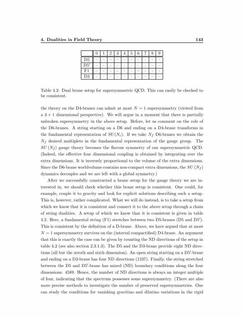
4. Dualities in Field Theory 143
0 1 2 3 4 5 6 7 8 9
D5 – – – – – – · · · ·D5′ – – – – · · · · – –
F1 – · · · · · – · · ·D3 – · · · · · · – – –
Table 4.2: Dual brane setup for supersymmetric QCD. This can easily be checked tobe consistent.
the theory on the D4-branes can admit at most N = 1 supersymmetry (viewed from
a 3 + 1 dimensional perspective). We will argue in a moment that there is partially
unbroken supersymmetry in the above setup. Before, let us comment on the role of
the D6-branes. A string starting on a D6 and ending on a D4-brane transforms in
the fundamental representation of SU(Nc). If we take Nf D6-branes we obtain the
Nf desired multiplets in the fundamental representation of the gauge group. The
SU (Nf) gauge theory becomes the flavour symmetry of our supersymmetric QCD.
(Indeed, the effective four dimensional coupling is obtained by integrating over the
extra dimensions. It is inversely proportional to the volume of the extra dimensions.
Since the D6-brane worldvolume contains non-compact extra dimensions, the SU (Nf )
dynamics decouples and we are left with a global symmetry.)
After we successfully constructed a brane setup for the gauge theory we are in-
terested in, we should check whether this brane setup is consistent. One could, for
example, couple it to gravity and look for explicit solutions describing such a setup.
This is, however, rather complicated. What we will do instead, is to take a setup from
which we know that it is consistent and connect it to the above setup through a chain
of string dualities. A setup of which we know that it is consistent is given in table
4.2. Here, a fundamental string (F1) stretches between two D5-branes (D5 and D5′).
This is consistent by the definition of a D-brane. Above, we have argued that at most
N = 1 supersymmetry survives on the (interval compactified) D4-brane. An argument
that this is exactly the case can be given by counting the ND directions of the setup in
table 4.2 (see also section 2.3.1.3). The D5 and the D3-brane provide eight ND direc-
tions (all but the zeroth and sixth dimension). An open string starting on a D5′-brane
and ending on a D3-brane has four ND directions (1237). Finally, the string stretched
between the D5 and D5′-brane has mixed (ND) boundary conditions along the four
dimensions: 4589. Hence, the number of ND directions is always an integer multiple
of four, indicating that the spectrum possesses some supersymmetry. (There are also
more precise methods to investigate the number of preserved supersymmetries. One
can study the conditions for vanishing gravitino and dilatino variations in the rigid

4. Dualities in Field Theory 144
NS5 NS5′
Nc D4
Nf D6
(Nf −Nc
)D4
Figure 4.3: Brane setup of figure 4.2 after pushing the D6-branes past the NS5 brane.
limit, see e.g. [158] for such an analysis within the present context.) It remains to see
that the setup in table 4.2 is connected to the one which we are interested in (table
4.1). Table 4.2 contains branes of type IIB theory. Therefore, we can apply an S-
duality (shortly described in the previous section) on this system. This takes the D5
and D5′-brane to the NS5 and NS5′ brane of table 4.1. The fundamental string (F1)
turns into a D1 string and the D3-brane remains invariant under S-duality. Performing
a T duality along the first, second and third dimension (replacing type IIB by IIA)
yields the configuration of table 4.1.
In the following we will describe a path in the moduli space of the setup in figure
4.2 taking us to the dual theory found by Seiberg. We will do so by essentially
interchanging the position of the NS5 with the NS5′ brane. This involves however
some subtleties which we will mention but not elaborate on. For more details we ask
the interested reader to consult[158] or literature to be given in chapter 6. Our first
step is to move the D6-branes to the left of the NS5 brane. When the D6-branes cross
the NS5 brane, Nf additional D4-branes stretching between the D6-branes and the
NS5 brane are created[238]. After the D6-branes have been moved to the left of the
NS5 brane, there is a point in moduli space where there are no D4-branes stretching
between the NS5 and the NS5′ brane. This can be achieved by connecting the Nc
D4-branes stretching between NS5′ and NS5 branes with Nc out of the Nf D4-branes
which stretch between D6-branes and NS5′ branes. The result of performing this first
step in moduli space is drawn in figure 4.3.
Now, the boundary conditions are such that we can displace the NS5 brane in the
seventh dimension. After doing so, it can be moved to the right of the NS5′ brane

4. AdS/CFT correspondence 145
Nf D4
Nf D6 NS5′ NS5
(Nf −Nc
)D4
Figure 4.4: Brane setup for the dual gauge theory.
along the sixth dimension.2 As soon as the NS5 brane is situated to the right of the
NS5′ brane, we realign it in the seventh dimension with the positions of the NS5′ and
the D4-branes. There are now (Nf −Nc) D4-branes starting at the D6-branes passing
through the NS5′ branes and ending on the NS5 brane. These we break on the NS5′
brane. The picture drawn in figure 4.4 emerges.
Finally, we need to read off the perturbative formulation of the field theory cor-
responding to figure 4.4. The gauge group of the theory living on the D4-branes
stretching between the NS5 and the NS5′ brane is SU (Nf −Nc). There are Nf chi-
ral multiplets in the fundamental of the gauge group coming from strings stretching
between the Nf D4-branes on the left and the Nf −Nc D4-branes in the middle. The
D4-branes to the left can move (fluctuate) in the eighth and ninth dimension. This
gives rise to N2f chiral multiplets which are singlets under the gauge group.
In this section we have seen that branes can be useful tools in deriving (or at least
illustrating) quite nontrivial connections between gauge field theories. Our purpose
was to provide the rough ideas on how this works within an example. The reader who
found this interesting is strongly advised to check the literature (chapter 6) for more
details and subtleties.
4.3 AdS/CFT correspondence
In this section we will describe a duality between gravity and field theory, or from a
stringy perspective between closed string excitations and open string excitations. We
will focus on the most prominent example where the field theory is N = 4 supercon-
2Here, it is important that the NS branes do not meet when passing each other.
4. The conjecture 146
formal SU (N) Yang-Mills theory3 (the theory of open string excitations ending on
D3 branes) and gravity lives on an AdS5×S5 space (the near horizon geometry of D3
branes). In the next subsection we will state the duality conjecture and mention the
most obvious consistency checks. Instead of elaborating on the various more involved
consistency checks which have been performed in the literature, we will discuss an
application of the duality. We will use the gravity side of the conjecture (the theory of
closed string excitations) to compute a Wilson loop in field theory. This will be done
in a semiclassical approximation. We will also discuss next to leading order correc-
tions. In order to avoid disappointment, we should mention here that we will not give
a quantitative result for the next to leading order corrections.
4.3.1 The conjecture
From section 3.3 we recall that in the case of the D3 branes the truncated action in
the Einstein frame and in the string frame look almost the same. We will work in the
string frame and absorb the constant dilaton into the definition of the gravitational
coupling κ. Choosing in addition a convenient4 numerical relation between α′ and κ,
we can write (see (3.3.0.23))
e−C = 1 +4πgsNα
′2
r4, (4.3.1.1)
where gs denotes the string coupling, and N = N3 is the number of D3 branes. Recall
also that the metric is (3.3.0.3) (use (3.3.0.6) and (3.3.0.7) and i, j = 0, . . . , 4, and we
parameterize the transverse space by polar coordinates, i.e. dΩ25 is the metric of a unit
five sphere)
ds2 = eC2 ηijdx
idxj + e−C2(dr2 + r2dΩ2
5
). (4.3.1.2)
Now we take the near horizon limit following the prescription
α′ → 0 and U ≡ r
α′fixed. (4.3.1.3)
The first limit ensures that the field theory on the brane decouples from gravity living
in the bulk. The second limit implies that we zoom in on the near horizon region. It
is taken such that the mass of an open string stretching between the N D3 branes and
3In order to distinguish between the number of branes and the number of supersymmetries we useN for the number of supersymmetries in the present section.
4The precise relation is (in Einstein frame units) κ2 = 16π7α′4, where Ω5 = π3 has been used(see (3.3.0.25)). Plugging this into (3.2.1.22), one finds that for this choice the NSNS charge of thefundamental string equals the RR charge of the D1 string (3.3.0.13). This implies that the numericsinvolved in the S duality of type IIB simplifies to gs → 1
gs.
4. The conjecture 147
some probe brane at a finite distance is constant. Performing the limit (4.3.1.3) the
metric (4.3.1.2) becomes5
ds2 = α′[
U2
√4πgsN
ηijdxidxj +
√4πgsN
dU2
U2+√
4πgsNdΩ25
]. (4.3.1.4)
This describes an AdS5×S5 geometry. Before taking a short detour on the description
of AdS5 spaces as hypersurfaces of a six dimensional space let us check the validity
region of (4.3.1.4) by focusing on the S5 part. The radius of the S5 is
R2 = α′√
4πgsN. (4.3.1.5)
In order to avoid high curvature (where higher derivative corrections become impor-
tant, or even the effective gravity description may break down) one should take this
radius to be large, i.e.
gsN 1. (4.3.1.6)
In addition we should keep the string coupling small which implies that the number
of D3 branes we look at has to be large. Now, we recall that the field theory living on
the D3 branes is N = 4 supersymmetric SU (N) gauge theory. The gauge coupling
is g2YM = 2πgs (see (2.3.3.22)). So, at first sight it seems that the gauge coupling
is small whenever the string coupling is small. However, we should also impose the
condition (4.3.1.6), in particular the large N limit. For large N SU (N) gauge theories
‘t Hooft developed a perturbative expansion in the parameter (the ‘t Hooft coupling)
g2YMN [435]. The condition (4.3.1.6) implies that the ‘t Hooft coupling is large when-
ever the effective gravity description is reliable. We will argue below that gravity (or
closed type IIB strings) in the space (4.3.1.4) is dual to the gauge theory living on
the D3 branes. Because of (4.3.1.6) this is a strong/weak coupling duality. One of
the first things one should check before publishing a conjecture on dual pairs is that
the global symmetries of the dual descriptions should match. (Global symmetries are
observable.) Therefore, let us take a short detour and describe the AdS5 space as a
hypersurface in a six dimensional space. This will enable us to see the isometries of
AdS5 in much the same way as one sees the SO (6) isometry of S5 when viewing it as
a hypersurface in six dimensional space.
The space in which we will find an AdSp+2 space as a hypersurface is a 2 + p + 1
dimensional space with the metric
ds2 = −dX2−1 − dX2
0 +
p+1∑
α=1
dX2α. (4.3.1.7)
5One can obtain this metric directly when dropping the requirement of an asymptotically trivialbackground in the search for BPS branes in section 3.3.
4. The conjecture 148
Analogously to a sphere, the AdSp+2 space is defined as the set of points satisfying
the condition
−X2−1 −X2
0 +
p+1∑
α=1
X2α = −R2, (4.3.1.8)
where R is called the radius of the AdSp+2 space. We solve this equation by
X−1 + Xp+1 = U, (4.3.1.9)
for i = 0, . . . , p: Xi = xiU
R, (4.3.1.10)
X−1 −Xp+1 =x2U
R2+R2
U, (4.3.1.11)
where x2 = ηijxixj and U and xi parameterize the hypersurface (4.3.1.8). Plugging
(4.3.1.9) – (4.3.1.11) into (4.3.1.7), we obtain the AdSp+2 metric
ds2 =U2
R2ηijdx
idxj + R2dU2
U2. (4.3.1.12)
Comparison with (4.3.1.4) shows us that the limit (4.3.1.3) took us to an AdS5 × S5
space where the radii of the AdS5 and the S5 coincide and are given by (4.3.1.5).
After this detour we can easily read of the isometries of (4.3.1.4). The isometry is
SO (4, 2)× SO (6). These isometries show up in the field theory on the D3 branes as
follows. The SO (6) (= SU (4)) is the R symmetry of N = 4 supersymmetric Yang-
Mills theory. The beta function of the gauge theory vanishes exactly, i.e. the gauge
theory is a conformal field theory. The SO (4, 2) part of the isometry corresponds to
the conformal group which is a symmetry in the gauge theory. Taking into account the
preserved supersymmetries6, one observes that the isometry group SO (4, 2)× SO (6)
can be extended to the superconformal group acting in the field theory. Thus the
global symmetries of the two descriptions match. In the asymptotic region U → ∞the AdS part of the metric (4.3.1.4) becomes (up to a conformal factor) the 3+1
dimensional Minkowski space. This is the boundary of the AdS space. The SO (4, 2)
isometry acts as the group of conformal transformations on the Minkowski space.
In this sense, one can identify the boundary of the AdS space with the location of
the D3 branes, although one should not think of the two descriptions simultaneously,
because whenever the parameters are such that the gravity description is reliable, the
perturbative description of the gauge theory breaks down and vice versa.
Moreover, one can identify the SL (2,Z) duality of the type IIB string with the
Montonen Olive duality[346, 463, 360, 457] of N = 4 super Yang Mills theory.
6These are enhanced in the near horizon limit.

4. Wilson loop computation 149
Thus, we have seen some evidence that the AdS/CFT correspondence conjecture
holds. More checks have been performed, but we will not discuss those here. In the
following section we want to illustrate the duality by computing Wilson loops in gauge
theory using type IIB superstrings. Before doing so, let us summarize the AdS/CFT
correspondence (duality) conjecture.
• Type IIB superstrings living in an AdS5 × S5 background are dual to open
superstrings ending on a stack of D3 branes.
• The AdS5 and the S5 have the same radius whose value (in units of α′) is
related to the ‘t Hooft coupling of the gauge theory via equation (4.3.1.5), and
g2YM = 2πgs.
• The type IIB string theory is in its perturbative regime if gs is small, and higher
curvature effects are not dangerous as long as (4.3.1.6) holds. In this region, the
gauge theory is in the large N limit and strongly coupled.
In a somewhat weaker statement, one should replace “type IIB superstrings” by “type
IIB supergravity” and “open strings ending on D3 branes” by N = 4 SU (N) gauge
theory. We will take the duality conjecture as stated in the items.
4.3.2 Wilson loop computation
4.3.2.1 Classical approximation
A Wilson loop is the (normalized) partition function of gauge theory in the presence
of an external quark anti-quark pair. A perturbative description of this situation in
a D3 brane setup for static quarks is drawn in figure 4.5. In order to employ the
AdS/CFT duality conjecture, we need to translate figure 4.5 to type IIB strings living
on AdS5 × S5. The prescription is that the open strings in figure 4.5 translate into
a background string of type IIB theory on AdS5 × S5. In the previous section we
have argued that the position of the N D3 branes is translated to the boundary of the
AdS5 space. (We should point out again that the emphasis is on “translated” since
the gauge theory description breaks down whenever the AdS prescription is reliable.)
Therefore, the background string should fulfill the boundary condition that its ends on
the AdS5 boundary are separated by a distance L. Classically, the background string
is then uniquely determined by the requirement of minimal worldsheet area. As we
will see in a moment, the picture drawn in figure 4.6 arises. The fact that the string
with minimal area goes down from the boundary into the AdS space and up again to
satisfy the boundary condition is a result of the non trivial metric. The corresponding

4. Wilson loop computation 150
D3 Brane
L
N
D3 Branes
single
Figure 4.5: The perturbative Wilson loop setup. The quark anti-quark pair cor-responds to the ends of open strings on the N D3 branes. The open strings have
opposite orientation. The quark anti-quark pair is chosen to be static. The dynamicsof the quarks decouples as long as the single D3 brane is very far away from the N D3
branes. The distance between the quark and the anti-quark is L.
String
Boundary
of AdS5
L
Background
Figure 4.6: The non perturbative Wilson loop setup. The quark anti-quark pair
corresponds to a background string ending on the AdS5 boundary.
4. Wilson loop computation 151
calculation can be carried out explicitly. For the sake of a minor simplification, we
redefine the coordinate U = R2
α′ u such that the metric (4.3.1.4) reads
ds2 = R2
[u2ηijdx
idxj +du2
u2+ dΩ2
5
]. (4.3.2.1)
The worldsheet area of the background string is
S =1
2πα′
∫dτdσ
√− det g (4.3.2.2)
where gαβ is the induced metric (2.1.1.2). As an ansatz for the background string we
take
X0 = τ , X1 = σ , X4 = U (σ) , (4.3.2.3)
and the rest of the string positions is constant in σ and τ . The indices are assigned in
the order in which coordinates appear in (4.3.2.1), and X4 = U (the capital U denotes
the string position in the space with the metric (4.3.2.1) and should not be confused
with the capital U in (4.3.1.3)). The first two equations in (4.3.2.3) represent the static
gauge and the sigma dependence of U allows for the string to describe the curve of
figure 4.6. This is the simplest consistent ansatz for the given boundary conditions.
The induced metric is
ds2ind
R2= −U2dτ2 +
(U2 +
(∂σU)2
U2
)dσ2. (4.3.2.4)
and thus the Nambu-Goto action (4.3.2.2) reads
S =TR2
2π
∫dσ
√(∂σU)2 + U4, (4.3.2.5)
where T denotes the time interval we are considering and we have set α′ to one (R2
is then a dimensionless quantity giving the AdS radius in units of α′). The action
(4.3.2.5) (and also the Lagrange density L obtained by dividing S by T ) does not
depend explicitly on σ. This implies
0 =∂L∂σ
= − (∂σU)∂L∂U−(∂2σU) ∂L∂ (∂σU)
+dLdσ
= − d
dσ
((∂σU)
∂L∂ (∂σU)
− L), (4.3.2.6)
where the Euler-Lagrange equations have been used in the last step. For our system
we obtain
∂σU = ±U2
U20
√U4 − U4
0 , (4.3.2.7)

4. Wilson loop computation 152
where U0 is a constant related to the integration constant of the last equation in
(4.3.2.6). U0 is the lower bound on the curve in figure (4.6) at σ = 0. Thus, we can
solve for σ as a function of U
σ = ±∫ U
U0
dUU2
0
U2
√U4 − U4
0
, (4.3.2.8)
where the plus-minus sign appears due to the two branches of the curve in figure 4.6
(σ is a horizontal coordinate and U a vertical one in this figure). At the boundary
(U →∞) the difference between the two values of σ should be L. Some straightforward
manipulations with the integral in (4.3.2.8) yield
L
2=
1
4U0B
(3
4,1
2
), (4.3.2.9)
where
B (α, β) =
∫ 1
0dxxα−1 (1− x)β−1 =
Γ (α) Γ (β)
Γ (α + β)
denotes Euler’s Beta function. Using the identities
xΓ (x) = Γ (x+ 1) , Γ (x) Γ (1− x) =π
sin πx, Γ
(1
2
)=√π
one finds for the integration constant
U0 =(2π)
32
Γ(
14
)2L. (4.3.2.10)
This shows our earlier statement that the background string is uniquely determined
by the boundary condition. The Wilson loop W [C] is the partition function for the
background string. For the classical approximation we find
W [C] = e−TE, (4.3.2.11)
with
E =R2
2π
∫dσ
√(∂σU)2 + U4. (4.3.2.12)
Plugging in the classical solution (4.3.2.7) (and taking into account a factor of two due
to the two branches) yields
E =R2
π
∫ ∞
U0
dUU2
√U4 − U4
0
. (4.3.2.13)
Now we split this integral into two pieces (the motivation for this will become clear
below)
E = Ec +Es, (4.3.2.14)

4. Wilson loop computation 153
with
Es =R2
π
∫ ∞
U0
dUU4 + U4
0
U2√U4 − U4
0
, (4.3.2.15)
and
Ec = −R2
π
∫ ∞
U0
dUU4
0
U2√U4 − U4
0
. (4.3.2.16)
Let us first discuss the integral Es. This integral is divergent due to the upper inte-
gration bound and we regularize it by a cutoff Umax. The asymptotic expansion for
large Umax is
Es =R2U0
π
∫ UmaxU0
1dy
y4 + 1
y2√y4 − 1
=R2U0
π
[√y4 − 1
y
]UmaxU0
1
=R2
πUmax + . . . , (4.3.2.17)
where the dots stand for terms going to zero as Umax is taken to infinity. Thus, Es
corresponds to the self energy of the two strings in figure 4.5. It does not depend on the
distance L and diverges as the length of the string is taken to infinity. Here, we observe
one interesting feature of the AdS/CFT correspondence. From the AdS perspective
Umax is a large distance, i.e. an IR cutoff. On the field theory side this appears as
a cutoff for high energies, i.e. a UV cutoff. This interchange between infrared and
ultraviolet cutoffs is a general characteristics of the correspondence[434]. Let us give a
technical remark in connection with the integral Es. Plugging in our classical solution
(4.3.2.7) into the induced metric (4.3.2.4), we find the classical value of the induced
metric (for later use we call this R2hαβ)
ds2class ≡ R2hαβdσ
αdσβ = R2
(−U2dτ2 +
U6
U40
dσ2
). (4.3.2.18)
The scalar curvature computed from hαβ reads
R(2) = 2U4 + U4
0
U4. (4.3.2.19)
With this information it is easy to verify that the structure of the self energy integral
is
Es =R2
4πT
∫d2σ√−hR(2). (4.3.2.20)
(This does not contradict the Gauss–Bonnet theorem because the worldsheet of the
background string is not compact.)

4. Wilson loop computation 154
Now, let us come to the second contribution in (4.3.2.14). This will turn out to be
the more interesting one. Its computation is quite similar to the computation of U0 in
terms of L. Therefore, let us just give the result
Ec = −4π2√
2g2YMN
Γ(
14
)4L
, (4.3.2.21)
where (4.3.1.5) and g2YM = 2πgs has been used. This is the part of the quark anti-quark
potential which arises due to gluon exchange among the two quarks. It is a Coulomb
potential. Since L is the only scale appearing in the setup and N = 4 supersymmetric
Yang–Mills theory has a conformal symmetry, there can be only a Coulomb potential.
Anything else would need another scale to produce an energy, but this cannot appear
due to conformal invariance.
In that respect models with less or none supersymmetry are more interesting be-
cause one can observe confinement in those models. The corresponding literature is
listed in chapter 6. The case we are considering here, is the one where the AdS/CFT
correspondence is perhaps best understood. We will study a question which is inter-
esting from a more theoretical perspective, namely whether there are corrections to
the result (4.3.2.21).
4.3.2.2 Stringy corrections
Before discussing corrections to (4.3.2.21) we should envisage the possibility that
(4.3.2.21) is an exact result. There are some results which may lead to this con-
clusion. By analyzing the structure of possible corrections to the AdS5×S5 geometry,
physicists[43, 340, 276] found that this geometry is exact. Still, there is a very simple
argument destroying the hope that (4.3.2.21) might be exact. Namely, the above Wil-
son loop computation can also be performed in the perturbative regime, where the ‘t
Hooft coupling is small. Then one finds, of course, also a Coulomb law but the depen-
dence on the ‘t Hooft coupling is linear instead of a square root dependence (which
actually cannot be obtained in a perturbative calculation). This does not contradict
the result (4.3.2.21) but tells us that taking the ‘t Hooft coupling smaller should result
in corrections such that finally for very small ‘t Hooft coupling the square root like
dependence goes over into a linear one.
After we have excluded corrections to the AdS5 × S5 geometry, we will study
fluctuations of the IIB string around the background string in figure 4.6. That is, we
consider the Wilson loop as the quantum mechanical partition function
W [C] =
∫[DδX ] [Dδθ] e−SIIB(X+δX,δθ), (4.3.2.22)

4. Wilson loop computation 155
where δX denote bosonic fluctuations and δθ fermionic ones (the fermionic background
of the string is trivial). Before going into the details of the computation, let us describe
the expansion we are going to perform. From (4.3.2.2) and (4.3.2.1) we see that the
square root of the ‘t Hooft coupling appears as an overall constant in front of the metric.
(This is also true for terms containing fermions.) Therefore, the expansion parameter ~(or α′ in section 2.1.3) is identified with the inverse square root of the ‘t Hooft coupling.
The expression (4.3.2.22) can be computed as a power series in this parameter. In
particular, the next to leading order correction to (4.3.2.21) will not depend on the ‘t
Hooft coupling. It is this correction we will discuss in some detail in the following. In
order to be able to use (4.3.2.22) for explicit calculations we need to know the type
IIB string action in an AdS5×S5 background. Fortunately, this has been constructed
in the literature[340]. These authors gave a type IIB action in the Green Schwarz
formalism, which is appropriate in the presence of non-trivial RR backgrounds. The
construction is similar to the one discussed in section 2.1.1.3. One uses target space
supersymmetry and kappa symmetry as a guide. The technicalities are rather involved
and we will not discuss them here. Because we will restrict ourselves to terms second
order in fluctuations we only need a truncated version of the action of type IIB strings
on AdS5 × S5. The complete action does not contain terms with an odd number of
target space fermions, in particular no terms linear in target space fermions. Since the
fermionic background is trivial, contributions quadratic in fluctuations can either have
two fermionic fluctuations and no bosonic fluctuation or only bosonic fluctuations.
The part of the action which is quadratic in the fluctuations consists of a sum of terms
with only bosonic fluctuations and terms with only fermionic fluctuations.
Let us discuss the bosonic fluctuations first. The type IIB action is a kappa
symmetric extension of (4.3.2.2). For the bosonic fluctuations only the contribution
(4.3.2.2) is relevant (for the lowest non trivial contribution). As in section 2.1.3 we pa-
rameterize the fluctuations by tangent vectors to geodesics connecting the background
with the actual value, i.e. we perform a normal coordinate expansion. The quantum
fields are
ξa = Eaµξµ, (4.3.2.23)
where Eaµ are the vielbein components obtained by taking the square root of the
diagonal metric components. A number as a label on a ξ will stand for a flat index
(a), unless stated explicitly otherwise. The computation of the term second order in
the ξa is a bit lengthy but straightforward with the information given in section 2.1.3.
(The only difference to section 2.1.3 is that we expand now a Nambu-Goto action
instead of a Polyakov action.) Before giving the result it is useful to perform a local

4. Wilson loop computation 156
ξµ=4
BackgroundString
ξµ=1
γ
x4 = u
x1 = σ
Figure 4.7: Perpendicular and longitudinal fluctuations in the one–four plane.
Lorentz rotation in the space spanned by the ξa. The rotation is7
(ξ‖
ξ⊥
)=
(cosα sinα
− sinα cosα
)(ξ1
ξ4
), (4.3.2.24)
with
cosα =U2
0
U2, sinα =
√U4 − U4
0
U2. (4.3.2.25)
Note that the determinant of the matrix appearing in (4.3.2.24) is one. The fields ξ‖
and ξ⊥ describe fluctuations parallel and perpendicular to the worldsheet, respectively.
This is illustrated in figure 4.7. Fluctuations drawn into figure 4.7 carry Einstein in-
dices which we indicated explicitly. The angle γ is given by the slope of the background
string
tanγ = ∂σU. (4.3.2.26)
The combination
ξµ=4 − tanγ ξµ=1 (4.3.2.27)
vanishes for
tanγ =ξµ=4
ξµ=1, (4.3.2.28)
7We employ the symmetry of the background string and take 0 ≤ σ ≤ L2 and the plus sign in
(4.3.2.7).

4. Wilson loop computation 157
i.e. if ξµ=1 + ξµ=4 is tangent to the background string. Thus, the combination in
(4.3.2.27) is normal to the background string. Transforming the indices to flat ones
(with the vielbein) and ortho-normalization yields ξ‖ and ξ⊥ with the given interpre-
tation. When writing down the Lagrangian second order in the fluctuations, we can
set R = 1 since we know the general R dependence (viz. none) from the argument
given above. The Lagrangian for the bosonic fluctuations comes out to be
L(2)bosons = L(2)
AdS5+ L(2)
S5 (4.3.2.29)
with
L(2)AdS5
=1
2
√−h
∑
a=2,3,⊥ξa∆ξa − 2
(ξ2)2 − 2
(ξ3)2
+(R(2) − 4
)(ξ⊥)2], (4.3.2.30)
L(2)S5 =
1
2
√−h
9∑
a′=5
ξa′∆ξa
′, (4.3.2.31)
where total derivative terms have been dropped (the fluctuations should satisfy Dirich-
let boundary conditions in order not to change the classical boundary conditions).
Further, ∆ denotes the two dimensional Laplacian with respect to the metric hαβ
(4.3.2.18) and R(2) is the corresponding scalar curvature (4.3.2.19). We observe that
the longitudinal fluctuations ξ0 and ξ‖ drop out of the action. Hence, we can fix the
worldsheet diffeomorphisms via
ξ0 = ξ‖ = 0. (4.3.2.32)
If the normalization of the functional integral in (4.3.2.22) contains a division by the
volume of the worldsheet diffeomorphisms, we cancel the ξ0 and ξ‖ integration against
this term in the normalization. This may be problematic, and we will comment on
this issue later.
It remains to study the fermionic fluctuations. Since the fermionic background is
trivial we just need to copy the Lagrangian from[340] (truncated to quadratic terms)
and to plug in our background. The result of the copying task is
LF = −1
2
√−hhαβ
(E aα − iθI γ a (Dαθ)
I)(
E aβ − iθJ γ a (Dβθ)
J)
−iεαβE aα
(θ1γ a (Dβθ)
1 − θ2γ a (Dβ)2). (4.3.2.33)
First, we need to explain some of the notation. The index a = 0, . . . , 9 labels the
tangent space coordinates of AdS5 × S5. Later, we will use an index a = 0, . . . , 4 for

4. Wilson loop computation 158
the tangent space of AdS5 and a′ = 5, . . . , 9 for the tangent space of S5. The vielbein
with a worldsheet index is
E aα = E a
µ∂αXµ, (4.3.2.34)
where Xµ is the position of the background string. The indices I, J = 1, 2 label the
two target space supersymmetries. The derivative Dα is defined as
(Dαθ)I =
[δIJ(∂α +
1
4(∂αX
µ)ωabµ γab
)− i
2εIJ (∂αX
µ)Eaµγ
a
]θJ
≡ ∇αθI −i
2εIJ (∂αX
µ)Eaµγ
aθJ . (4.3.2.35)
Here, ωabµ denotes the target space spin connection and we have used the fact that our
background is trivial in S5 directions. The gamma matrices γ a =(γa, iγa
′)
satisfy
SO (4, 1) and SO (5) Clifford algebras, respectively. The θI are sixteen component
spinors each. They are conveniently labeled by a double spinor index θαα′
where α is
a spinor index in the tangent space of the AdS5, and α′ a spinor index in the tangent
space of S5. The γa and γa′
are four times four matrices tensored with four times
four identity matrices. (In the following we will suppress target space spinor indices
in order to avoid confusion with worldsheet indices which are also labeled by small
Greeks.)
We do not intend to give a derivation of (4.3.2.33) but let us have a brief look
at its structure before proceeding. Expression (4.3.2.35) is a tensor (density) with
indices αβ contracted either with hαβ or εαβ . The terms with hαβ can be thought
of as arising from the replacement (2.1.1.36)8 whereas the εαβ contracted terms come
from the Wess Zumino term (2.1.1.38) needed for kappa symmetry. The details differ
from the discussion in section 2.1.1.3 due to the different target space geometry and
the RR four form flux.
For our background, the Lagrangian (4.3.2.33) can be written in a compact way
LF = −√−h(θ1, θ2
)(
2iEaµ (∂αX
µ)γaPαβ− ∇β 1− B−1− B 2iEa
µ (∂αXµ) γaPαβ+ ∇β
)(θ1
θ2
), (4.3.2.36)
where Xµ stands for the background position of the string and
Pαβ± =1
2
(hαβ ± εαβ√
−h
), (4.3.2.37)
B =1
2√−h
εαβEaµE
bν (∂αX
µ) (∂βXν)γab. (4.3.2.38)
8In general, the combination in (2.1.1.36) contains also terms higher than quadratic order in thefermions. This is because the superalgebra is altered in the AdS5 × S5 case as compared to a flattarget space. This should be clear by noting that the isometries form a subgroup of the supersymmetrytransformations.
4. Wilson loop computation 159
As usual, a gamma with a multiple index is the antisymmetrised product of gamma
matrices.
It is useful to perform the rotation (4.3.2.24) also on the spinors (with α as given
in (4.3.2.25))
θI =(
cosα
2− sin
α
2γ14)ψI . (4.3.2.39)
In order to compute the partition function, we should fix the kappa symmetry. This
is conveniently done in terms of the nilpotent matrices
γ± =1
2
(γ0 ± γ1
). (4.3.2.40)
In analogy to section 2.1.1.3, we choose the kappa fixing conditions
γ−ψ1 = 0 , γ+ψ2 = 0. (4.3.2.41)
We assume that the integration over spinors not satisfying (4.3.2.41) cancels the volume
of kappa transformations appearing as a normalization factor in the functional integral.
This may be problematic, and we will comment on this issue later. Spinors satisfying
the kappa fixing condition are then governed by the Lagrangian
LF = −√−h(ψ1, ψ2
)(iγ+∇+ 2
−2 iγ−∇−
)(ψ1
ψ2
), (4.3.2.42)
where ∇± are tangent space derivatives defined as follows
∇± = eτ0∇τ ± eσ1∇σ =1
U∇τ ±
U20
U3∇σ, (4.3.2.43)
where eτ0 and eσ1 are two dimensional (inverse) vielbein components obtained from the
square roots of the diagonal elements of hαβ. Note also that the covariant derivative
simplifies when acting on spinors satisfying (4.3.2.41). Defining partial tangent space
derivatives analogously to (4.3.2.43) one finds
∇±ψI =(∂± ±
ω±2
)ψI , (4.3.2.44)
where
ω± = eτ0ω01τ ± eσ1ω01
σ (4.3.2.45)
are tangent space components of the two dimensional spin connection ω01α computed
from the zweibeinen defined in (4.3.2.43). Let us further define the matrices
ρ+ =
(0 0
γ0 0
), ρ− =
(0 −γ0
0 0
). (4.3.2.46)

4. Wilson loop computation 160
These are the same matrices as in (2.1.1.17) with i replaced by γ0/2. Finally, we
rewrite (4.3.2.42) in a suggestive way as follows
LF = −√−h(ψ2, −ψ1
)(
−2 iγ−∇−−iγ+∇+ −2
)(ψ1
ψ2
)
= −√h(ψ2, −ψ1
)(
−2 2iγ0∇−−2iγ0∇+ −2
)(ψ1
ψ2
)
= 2√−h(ψ2, −ψ1
)(iρm∇m + 1)
(ψ1
ψ2
), (4.3.2.47)
where in the second line (4.3.2.41) has been used and a repeated index m stands
for the sum over the labels + and −. Comparison with the expressions in section
2.1.1.2 shows that the part of the action containing target space spinor fluctuations
‘metamorphosed’ into an action for worldsheet spinors after imposing the kappa fixing
condition (4.3.2.41). The difference is that the derivative contains the spin connection
due to the non trivial worldsheet metric hαβ (4.3.2.18), and the mass terms appearing
due to the constant non vanishing curvature of the AdS space.
Now we have collected all the information needed to express the second order fluctu-
ation contribution to (4.3.2.22) in terms of determinants of two dimensional differential
operators. (For Dirac operators one uses the formal identity detA =√
detA2.)
Integration over the fluctuations leads to determinants of operators which can be
read off from (4.3.2.30), (4.3.2.31) and (4.3.2.47). The corrected expression for the
Wilson loop reads
W [C] = e−TEclassdet(−∆F − 1
4R(2) + 1
)
det (−∆ + 2) det12(−∆ + 4− R(2)
)det
52 (−∆)
. (4.3.2.48)
The exponential is the classical contribution with Eclass given by (4.3.2.14), (4.3.2.20)
and (4.3.2.21). Note also that the operator appearing in the numerator of (4.3.2.48) is a
four times four matrix. The Laplacian acting on worldsheet fermions ∆F is ηmn∇n∇m.
Unfortunately it is not known how to evaluate the determinants in (4.3.2.48) exactly.
What is known exactly are the divergent contributions. These are given in (2.1.3.33).
They are of the form
Ediv ∼∫d2σ√−hR(2). (4.3.2.49)
Comparing with (4.3.2.20), we find that this divergence renormalizes the self-energy
which is infinite anyway. A correction to the Coulomb charge of the quarks will be
finite. Unfortunately, we cannot give it in a more explicit way (as a number).
In addition, there is also a conceptual puzzle with the divergent contribution.
Although for our problem it is not relevant, it should not be there. The argument

4. Strings at a TeV 161
that something might have gone wrong goes as follows. The string action is equivalent
to a Polyakov type action, at least at a classical level (see section (2.1.1.1)). The
Polyakov action is conformally invariant, and in a consistent string background the
conformal invariance should not be broken by quantum effects. Therefore, divergences
which introduce a cutoff (or renormalization group scale) cannot occur. Indeed, it
was argued in[149] that a treatment analogous to ours but with a Polyakov instead
of the Nambu-Goto action leads to a finite result. This treatment is a bit more
complicated since the worldsheet metric appears as an independent field which also
fluctuates. The advantage is however that subtle contributions due to the occurring
integral measures are well understood. Such contributions are typically of the structure
(4.3.2.49)[16, 193, 328]. (Note, however, that if the worldsheet metric is identified with
the induced metric, the term in (4.3.2.49) is not really distinguishable from (∂X)2
terms (see e.g.[155])). In our derivation, we have mentioned already two places where
nontrivial measure contributions could arise. This could happen when we cancel the
integration over the longitudinal fluctuations against the volume of the worldsheet
diffeomorphisms and in the kappa fixing procedure. Unfortunately, the Nambu-Goto
case is less understood than the Polyakov formulation. (For a recent attempt to fix
the functional measures in the bosonic part see[347].) Fortunately, the result of the
better understood calculation in the Polyakov approach is identical to the one given
here (up to the irrelevant divergence)[149].
With these open questions we close our discussion on the AdS/CFT correspon-
dence. The reader who wants to know more will find some references in chapter 6.
4.4 Strings at a TeV
So far we have not determined the numerical value of the string scale (set by α′) in
terms of a number. We restricted our discussions mostly to the massless excitations
of the string. This was motivated by the belief that the string scale (in energies)
is large compared to observed energy scales. Often it is comparable to the Planck
scale. This identification is motivated by studies of heterotic weakly coupled strings
which provided for a long time the most promising starting point in constructing
phenomenologically interesting models. Such models are obtained by compactifying
the ten dimensional heterotic (mostly E8 × E8) string down to four dimensions on a
Calabi–Yau manifold. Let us give a rough estimate for the resulting four dimensional
couplings. The effective four dimensional heterotic action is of the form
Shet =
∫d4x
V
g2h
(l−8h R(4) − l−6
h trF 2 + . . .), (4.4.0.1)
4. Strings at a TeV 162
where we drop details which are not relevant for the present estimate on scales. In
(4.4.0.1) lh is the heterotic string scale (set by α′), gh the heterotic string coupling
(fixed by the dilaton vev), and V is the volume of the compact space. The quantities
in which four dimensional physics is usually described are the four dimensional Planck
mass Mp and the gauge coupling gYM . These are related to the input data (gh, lh and
V ) as follows
M2p =
V
g2hl
8h
,1
g2YM
=V
g2hl
6h
. (4.4.0.2)
Expressing gh in the first equation in terms of the second equation and further defining
the string mass scale as Mh = 1/lh the above equation can be rewritten as
Mh = gYMMp , gh = gYM
√V
l3h. (4.4.0.3)
Now we assume that a gYM ∼ 0.2 is a realistic value. (This is the gauge coupling of
the minimal supersymmetric standard model at the GUT scale.) Plugging gYM = 0.2
into the first equation in (4.4.0.3) we find that the heterotic string scale is
Mh ∼ 1018GeV, (4.4.0.4)
i.e. of the order of the Planck scale. The second equation in (4.4.0.3) implies that the
compact space is also of the Planck size if we want to stay within the region where the
string coupling is small.
Now let us investigate how the above estimates on scales are altered in a the-
ory containing branes. Phenomenologically interesting models arise also as orientifold
compactifications of type II theories. As we have seen in section 2.4, these contain typ-
ically D-branes on which the gauge interactions are localized whereas the gravitational
sector corresponds to closed string excitations which propagate in all dimensions. As-
suming that the gauge sector (and charged matter) is confined to live on Dp-branes
the effective action for the orientifold compactification will be of the form
Sori =
∫d10x
1
g2II l
8II
R−∫dp+1x
1
gII lp−3II
trF 2, (4.4.0.5)
where lII and gII are the string scale and coupling of the underlying type II theory,
respectively. Assuming further that our orientifold construction is such that the com-
pact space has dimensions which are transverse to all relevant D-branes we denote by
V⊥ the volume of the compact space transverse to the branes and by V‖ the volume of
the compact space longitudinal to the branes (such that the overall compact volume
is V = V⊥V‖). With this notation the four dimensional action reads
Sori =
∫d4x
V‖V⊥g2II l
8II
R−∫d4x
V‖gIIl
p−3II
trF 2, (4.4.0.6)
4. Strings at a TeV 163
from which we obtain the four dimensional Planck length lp and gauge coupling gYM
1
l2p=V‖V⊥g2IIl
8II
,1
g2YM
=V‖
gII lp−3II
. (4.4.0.7)
Hence, the four dimensional Planck mass (Mp = 1/lp) and the string coupling gII are
M2p =
v⊥l−2II
v‖ (gYM )4 , gII = g2YMv‖, (4.4.0.8)
where
v‖ = V‖ l3−pII , v⊥ = V⊥ l
p−9II (4.4.0.9)
are dimensionless numbers describing the size of the compact space in string scale
units. The relations (4.4.0.8) allow to take the string length lII larger than the four
dimensional Planck length lp. This can be achieved by taking v⊥ large. The size of the
parallel volume is taken to be of the “string size”, i.e. v‖ ∼ 1. If the parallel volume is
smaller than the string size, we T-dualize with respect to the smaller dimension. This
dimension will then contribute to the perpendicular volume since the string changes
boundary conditions. Hence, the v‖ < 1 case is T dual to the considered case of large
v⊥. On the other hand if v‖ > 1, the second equation in (4.4.0.8) tells us that in this
case the string coupling becomes strong, and our description breaks down. (Moreover,
it is problematic for gauge interactions to be compactified on large volumes because
the corrections to the four dimensional gauge interactions are usually ruled out by
experimental accuracy.)
Let us analyse in some detail what happens if we choose a TeV for the string scale.
This is about the lowest value which is just in agreement with experiments. (For a
lower value massive string excitations should have shown up in collider experiments.)
With Mp ∼ 1016TeV we find
v⊥ ∼ 1028 → V⊥ = 1028 1
(TeV)9−p . (4.4.0.10)
The Planck length is about 10−33cm and hence in our units one TeV corresponds to
1/(10−18m
). Thus we obtain
V⊥ ∼ 1028−(9−p)18 (m)9−p . (4.4.0.11)
For the case p = 8 (one extra large dimension) we obtain that the perpendicular
dimension is compactified on a circle of the size
p = 8 → R⊥ ∼ 1010km. (4.4.0.12)

4. Strings at a TeV 164
Such a value is certainly excluded by observations. (In the next subsection we will
compute corrections to Newton’s law due to Kaluza-Klein massive gravitons and see
that the size of the compact space should be less than a mm.) For p = 7 we obtain
(distributing the perpendicular volume equally on the two (extra large) dimensions)
p = 7→ R⊥ ∼ 0.1mm. (4.4.0.13)
This value is just at the edge of being experimentally excluded. The situation improves
the more extra large dimensions there are. For example in the case p = 3 (and again
a uniform distribution of the perpendicular volume on the six dimensions (V⊥ = R6⊥))
we obtain
p = 3 → R⊥ ∼ 10−10m, (4.4.0.14)
which is in good agreement with the experimental value (Rexp⊥ = 0...0.1mm).
We have seen that D branes allow the construction of models where the string
scale is as low as a TeV. (Note also, that in the above discussion we can perform
T-dualities along the string sized parallel dimensions. This changes p but leaves the
large extra dimensions unchanged. Actually, it might be preferable to have p = 3 in
order to avoid Kaluza–Klein gauge bosons of a TeV mass.) This gives the exciting
perspective that string theory might be at the horizon of experimental discovery. In
near future collider experiments, massive string modes would be visible. In addition,
the extra large dimensions could be also discovered soon. This can happen either by
the production of Kaluza-Klein gravitons in particle collisions or by short distance
Cavendish like experiments. However, it might as well be the case that models with
less “near future discovery potential” are realized in nature.
Apart from the prospect of being observed soon, strings at a TeV scale are interest-
ing for another reason. If the string scale is at a TeV, we would call this a fundamental
scale. Thus the hierarchy problem would be rephrased. With the fundamental scale at
a TeV we should wonder why the (four dimensional) Planck scale is so much higher, or
why gravitational interactions are so much weaker than the other known interactions.
This hierarchy is now attributed to the size of the extra large dimensions. Super-
symmetry may not be necessary to explain the hierarchy between the Planck scale
and the weak scale. Therefore, in the above models supersymmetry could be broken
already by the compactification. In such models the question of stability is typically
a problematic issue.
The above considerations are also interesting if one does not insist on a direct
connection to string theory. If one just starts ‘by hand’ with a higher dimensional
setup containing branes, one would also obtain the first equation in (4.4.0.8). In this
4. Corrections to Newton’s law 165
case, one calls lII the higher dimensional Planck length, which in turn can be chosen
to be 1/TeV.
4.4.1 Corrections to Newton’s law
In the previous section we stated that observations provide experimental bounds on
the size of extra dimensions. In the brane setup in which we found the possibility of
large (as compared to the Planck length) extra dimensions, these extra dimensions
are typically tested only by gravitational interactions. Therefore, let us describe the
influence of additional dimensions on the gravitational interaction in some more detail.
We will be interested in the Newtonian limit of gravity. For simplicity, we assume that
the space is of the structure M4 × Tn, where M4 is the 3 + 1 dimensional compact
space and Tn is an n dimensional torus of large volume. (There might be an additional
compact space of Planck size. This does not enter the computation carried out below.)
The analysis we will carry out here is similar to the discussion of the massless scalar
in section 2.1.5.1, where the role of the scalar is taken over by the Newton potential.
Let us arrange the spatial coordinates into a vector (x,y), where x corresponds to
the M4 and y to the Tn. For simplicity we assume that the torus is described by a
quadratic lattice and the uniform length of a cycle is 2πR, i.e.
y ≡ y + 2πR. (4.4.1.15)
The n+ 4 dimensional Newton potential Vn+4 of a point particle with mass µ located
at the origin is given by the equation
∆n+3Vn+4 = (n+ 1) Ωn+2Gn+4 µ δ(n+3) (x,y) , (4.4.1.16)
where ∆n+3 is the three dimensional flat Laplacian and Ωn+2 is the volume of a unit
n+ 2 sphere. Any solution to (4.4.1.16) should be periodic under (4.4.1.15). This can
be ensured by expanding the potential in terms of eigenfunctions ψ k (y) of a Laplace
operator. The eigenvalue equation is
∆nψk (y) = −m2kψk (y) . (4.4.1.17)
Thus an orthonormal set of eigenfunctions is
ψk =1
(2πR)n2
eikRy, (4.4.1.18)
where k is an n dimensional vector with integer entries. We expand the higher di-
mensional Newton potential into a series of the eigenfunctions with r = |x| dependent
coefficients
Vn+4 =∑
k
φk (r)ψk (y) . (4.4.1.19)
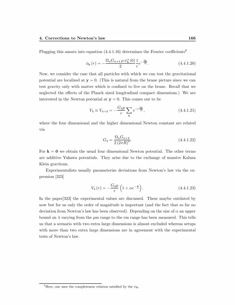
4. Corrections to Newton’s law 166
Plugging this ansatz into equation (4.4.1.16) determines the Fourier coefficients9
φk (r) = −ΩnGn+4 µψ?k (0)
2
1
re−|k|R . (4.4.1.20)
Now, we consider the case that all particles with which we can test the gravitational
potential are localized at y = 0. (This is natural from the brane picture since we can
test gravity only with matter which is confined to live on the brane. Recall that we
neglected the effects of the Planck sized longitudinal compact dimensions.) We are
interested in the Newton potential at y = 0. This comes out to be
V4 ≡ Vn+4 = −G4µ
r
∑
k
e−r|k|R , (4.4.1.21)
where the four dimensional and the higher dimensional Newton constant are related
via
G4 =ΩnGn+4
2 (2πR)n. (4.4.1.22)
For k = 0 we obtain the usual four dimensional Newton potential. The other terms
are additive Yukawa potentials. They arise due to the exchange of massive Kaluza
Klein gravitons.
Experimentalists usually parameterize deviations from Newton’s law via the ex-
pression [323]
V4 (r) = −G4µ
r
(1 + αe−
rλ
). (4.4.1.23)
In the paper[323] the experimental values are discussed. These maybe outdated by
now but for us only the order of magnitude is important (and the fact that so far no
deviation from Newton’s law has been observed). Depending on the size of α an upper
bound on λ varying from the µm range to the cm range has been measured. This tells
us that a scenario with two extra large dimensions is almost excluded whereas setups
with more than two extra large dimensions are in agreement with the experimental
tests of Newton’s law.
9Here, one uses the completeness relation satisfied by the ψk.
Chapter 5
Brane world setups
In the last section of the previous chapter we have argued that branes allow for scenar-
ios with large extra dimensions transverse to the brane. This is because those extra
large dimensions can be tested only via gravitational interactions which are (due to
their weakness) measured only at scales down to about 0.1 mm. We obtained such
models via investigations of string theory. One could, however, just postulate the exis-
tence of branes (on which charged interactions are located). In this last chapter we will
take this latter point of view and not worry whether the setups we are going to discuss
have a stringy origin. Because in the presence of branes we can attribute the hierarchy
between the Planck and the weak scale to the size of the transverse dimensions, we
do not need supersymmetry in such setups. Without supersymmetry, quantum effects
usually create vacuum energies. A non vanishing vacuum energy on a brane will back
react on the geometry of the space in which the brane lives. Taking into account such
back reactions leads to so called warped compactifications. This means that the higher
dimensional geometry is sensitive to the position of a brane. The most prominent ex-
ample of such warped compactifications are the Randall Sundrum models which we
will discuss next.
5.1 The Randall Sundrum models
5.1.1 The RS1 model with two branes
In the model we are going to describe in this section there is one extra dimension which
will be denoted by φ. The five dimensional space is a foliation with four dimensional
Minkowski slices. The fifth dimension is compactified on an orbifold S1/Z2. 3-branes
are located at the orbifold fixed planes (at φ = 0 and φ = π) . Hence the action is of
167

5. The RS1 model with two branes 168
the form
S = Sbulk + Sb1 + Sb2, (5.1.1.1)
where Sb1 and Sb2 denote the actions on the branes. For the bulk action we take five
dimensional gravity with a bulk cosmological constant,
Sbulk =
∫d4x
∫ π
−πdφ√−G
(2M3R− Λ
), (5.1.1.2)
where M denotes the five dimensional Planck mass and GMN is the five dimensional
metric. The branes are located in φ and we identify the brane coordinates with the
remaining 5d coordinates xµ, µ = 0, . . . , 3. Then the induced metrics on the branes
are simply
gb1µν = Gµν |φ=0 , gb2µν = Gµν |φ=π . (5.1.1.3)
We assume that fields being localized on the brane are in the trivial vacuum and
take into account only nonzero vacuum energies on the branes. Calling those vacuum
energies T1 and T2, the brane actions read
Sb1 + Sb2 = −∫d4x
(T1
√−gb1 + T2
√−gb2
), (5.1.1.4)
where the first (second) term on the lhs is attributed to the first (second) term on
the rhs. Instead of working out the solutions to the system on an interval S1/Z2 it
is technically easier to construct a solution in a non compact space, such that the
solution is periodic in
φ ≡ φ+ 2π, (5.1.1.5)
and even under
φ→ −φ. (5.1.1.6)
A vacuum with this property yields then automatically a compact interval in φ. (The
equivalent1 and more complicated alternative is to define the theory on an interval from
the very beginning and take into account surface terms when deriving the equations
of motion as well as Gibbons Hawking[200] boundary terms (for a discussion in the
context of brane worlds see also[132, 133]).) With these remarks the Einstein equations
of motion read (capital indices run over all dimensions M,N = 0, . . . , 4)
√−G
(RMN −
1
2GMN
)=
− 1
4M3
[Λ√−GGMN +
2∑
i=1
Ti√−gbigbiµνδµM δνN δ (φ− φi)
], (5.1.1.7)
1I acknowledge discussions with Rados law Matyszkiewicz on this topic.

5. The RS1 model with two branes 169
−π
|φ|
φ
π0−2π
Figure 5.1: The periodic modulus function.
with φ1 = 0 and φ2 = π. The delta functions appearing on the rhs of (5.1.1.7) are
defined on a real line. The most general metric ansatz possessing a four dimensional
Poincare transformation as isometry is
ds2 = e−2σ(φ)ηµνdxµdxν + r2
cdφ2. (5.1.1.8)
We could rescale φ such that the rc dependence drops out, but that would change
the periodicity condition (5.1.1.5). Plugging this ansatz into the equations of motion
(5.1.1.7) yields (a prime denotes differentiation with respect to φ)
6σ′2
r2c
= − Λ
4M3, (5.1.1.9)
3σ′′
r2c
=T1
4M3rcδ (φ) +
T2
4M3rcδ (φ− π) . (5.1.1.10)
The solution to (5.1.1.9) is
σ = rc |φ|√−Λ
24M3, (5.1.1.11)
where the modulus function is defined as usual in the interval −π < φ < π,
|φ| =−φ , −π < φ < 0
φ , 0 < φ < π. (5.1.1.12)
This ensures that the solution is even under φ → −φ. In order to incorporate
(5.1.1.5), we define the modulus function on the real line by the periodic continu-
ation of (5.1.1.12). The resulting function is drawn in figure 5.1. Away from the
points at φ = 0 and integer multiples of π, the second derivative of σ vanishes and

5. The RS1 model with two branes 170
(5.1.1.10) is fulfilled in those regions. In order to take into account the delta function
sources in (5.1.1.10), one integrates this equation over an infinitesimal neighborhood
around the location of the brane sources. This gives rise to the constraints
T1 = −T2 = 24M3k ,with k2 = − Λ
24M3(5.1.1.13)
on the parameters of the model. These constraints can be thought of as fine tuning
conditions for a vanishing effective cosmological constant in four dimensions. We will
come back to this point in section 5.2.3. Our final solution is
ds2 = e−2krc |φ|ηµν + r2cdφ
2, (5.1.1.14)
where k2 is defined in (5.1.1.13), and we take k to be positive (for a negative k just
redefine φ→ π − φ).
We observe that by taking into account the back reaction of the branes onto the
geometry, we obtain a metric which depends on the position in the compact direction.
For the particular model we consider this dependence is exponential. That opens up
an interesting alternative explanation for the large hierarchy between the Planck scale
and the weak scale. We take all the input scales (M , Λ , rc) to be of the order of the
Planck scale. First, we should check whether this provides the correct four dimensional
Planck mass. To this end, we expand a general 4d metric around the classical solution
ds2 = e−2krc (ηµν + hµν)dxµdxν + r2cdφ
2. (5.1.1.15)
In principle we should also allow the four-four component of the metric r2c to fluctuate.
Since rc is an integration constant, such fluctuations will be seen as massless scalars
in the effective four dimensional theory. This is a common problem known as moduli
stabilization problem. We will assume here that some unknown mechanism gives a
mass to the fluctuations of G44 and take it to be frozen at the classical value r2c . The
Kaluza-Klein gauge fields Gµ4 are projected out by the Z2. Plugging (5.1.1.15) into the
action and integrating over φ yields the effective action for four dimensional gravity
Seff = M2p
∫d4x√−gR(4) (g) , (5.1.1.16)
where R(4) (g) denotes the four dimensional scalar curvature computed from gµν =
ηµν + hµν and the four dimensional Planck mass Mp is given by
M2p = M3rc
∫ π
−πdφe−2krc|φ| =
M3
k
(1− e−2krcπ
). (5.1.1.17)
This tells us that choosing five dimensional scales of the order of the Planck scale gives
the correct order of magnitude for the four dimensional Planck scale.
5. The RS1 model with two branes 171
Now, let us consider matter living on the branes. On the first brane located at
φ = 0, the induced metric is just the Minkowski metric and Lagrangians for matter
living on that brane will just have their usual form. On the other hand, matter living
on the second brane (located at φ = π) feels the φ dependence of the bulk metric. Let
us focus on a Higgs field being located at the second brane. Its action will be of the
form
Sb2Higgs =
∫d4xe−4krcπ
e2krcπηµνDµH
†DνH − λ(|H |2 − v2
o
)2, (5.1.1.18)
where the overall exponential factor originates from the determinant of the induced
metric. Rescaling the Higgs field H such that the kinetic term in (5.1.1.18) takes its
canonical form induces the rescaling
v0 → veff = e−krcπv0. (5.1.1.19)
This means that a symmetry breaking scale which is written as v0 into the model
effectively is multiplied by a factor of e−krcπ . Repeating the above argument for any
massive field, one finds that any mass receives such a factor
m0 → meff = e−krcπm0, (5.1.1.20)
when going to an effective description in which kinetic terms are canonically normal-
ized. Choosing krc ≈ 10 (which is roughly a number of order one), one can achieve
that the exponential in (5.1.1.20) takes Planck sized input masses to effective masses
of the order of a TeV. Hence, in the above model we can obtain the TeV scale from
the Planck scale without introducing large numbers, provided we live on the second
brane.
5.1.1.1 A proposal for radion stabilization
In the previous section, we have already mentioned that the internal metric component
G44 gives rise to a massless field in an effective description. This means that its vev
rc is very sensitive against any perturbation and rather unstable. For the discussion
of the hierarchy problem it is important that the distance of the branes rc is of the
order of the Planck length. Therefore, it is desirable to stabilize this distance, i.e.
to give a mass to G44 in the effective description. In the present section we briefly
present a proposal of Goldberger and Wise how a stabilization might be achieved via
an additional scalar living in the bulk. We will neglect the back reaction of the scalar
field on the geometry. This means that we just consider a scalar field in the RS1
background constructed in the previous section. The action consists out of three parts
S = Sbulk + Sb1 + Sb2, (5.1.1.21)
5. The RS1 model with two branes 172
where Sbulk defines the five dimensional dynamics of the field and Sb1 and Sb2 its
coupling to the respective branes. We choose
Sbulk =1
2
∫d4x
∫ π
−πdφ√−G
(GMN∂MΦ∂NΦ−m2Φ2
), (5.1.1.22)
where Φ is the scalar field and GMN is given in (5.1.1.14). The coupling to the branes
is taken to be
Sb1 = −∫d4x√−gb1λ1
(Φ2 − v2
1
)2, (5.1.1.23)
Sb2 = −∫d4x√−gb2λ2
(Φ2 − v2
2
)2, (5.1.1.24)
where vi and λi are dimensionfull parameters whose values will be discussed below.
With the ansatz that Φ does not depend on the xµ for µ = 0, . . . , 3 the equation of
motion for the scalar is
e−4krc|φ|(−e
4krc |φ|
r2c
∂φ
(e−4krc |φ|∂φΦ
)+m2Φ
+4λ1Φ(Φ2 − v2
1
) δ (φ)
rc+ 4λ2Φ
(Φ2 − v2
2
) δ (φ− π)
rc
)= 0. (5.1.1.25)
With ν =√
4 + m2
k2 the solution inside the bulk 0 < φ < π is written as
Φ = e2krc|φ|(Aekrcν|φ| +Be−krcν|φ|
), (5.1.1.26)
where the integration constants A and B will be fixed below. Plugging this solution
back into the Lagrangian yields an rc dependent constant, i.e. a potential for the
distance of the two branes,
V (rc) = k (ν + 2)A2(e2νkrcπ − 1
)+ k (ν − 2)B2
(1− e−2νkrcπ
)
+λ1
(Φ (0)2 − v2
1
)2+ λ2e
−4krcπ(
Φ (π)2 − v22
)2. (5.1.1.27)
Because of the dependence of Φ on the modulus function (see figure 5.1) the second
derivative in the first term in (5.1.1.25) will lead to delta functions whose argument
vanishes at the position of the branes. Matching this with the delta function source
terms in (5.1.1.25) yields equations for the integration constants A and B. Instead
of writing down and solving those equations explicitly we suppose that λ1 and λ2 are
large enough for the approximation
Φ (0) = v1 , Φ (π) = v2 (5.1.1.28)

5. The RS1 model with two branes 173
to be sufficiently accurate. In this approximation one obtains
A = v2e−(2+ν)krcπ − v1e
−2νkrcπ, (5.1.1.29)
B = v1
(1 + e−2νkrcπ
)− v2e
−(2+ν)krcπ. (5.1.1.30)
The next approximation lies in the assumption that
ε =m2
4k 1. (5.1.1.31)
In evaluating the potential V (rc) (5.1.1.27), we neglect terms of order ε2 but do not
treat εkrc as a small number. This yields
V (rc) = kεv21 + 4ke−4krcπ
(v2 − v1e
−εkrcπ)2 (
1 +ε
4
)
−kεv1e−(4+ε)krcπ
(2v2 − v1e
−εkrcπ). (5.1.1.32)
Up to orders of ε, this potential has a minimum at
krc =4k2
πm2log
(v1
v2
). (5.1.1.33)
In figure 5.2, we have drawn the potential in a neighborhood of the minimum (using
Maple). (What is actually drawn is V − kεv21 .) With the appropriate choice for the
scales, the minimum of the potential is clearly visible. One should note, however, the
exponentially suppressed height of the right wall of the potential. If we had chosen
a larger scale for the drawing, figure 5.2 would just show a runaway potential which
rapidly reaches its asymptotic value. This might be a drawback of the stabilization
mechanism.
The expression for the stable distance between the branes (5.1.1.33) shows that
no extreme fine tuning is needed in order to obtain the wanted value of about ten
for krc. It remains to investigate whether the various approximations (including the
neglection of the back reaction) are sensible. This investigation has been carried out
in[215] by estimating the size of next to leading order corrections. The result is that
the approximations are fine.
To close this section, we should mention that the described stabilization method
is often called “Goldberger Wise mechanism” in the literature. We preferred to use
the term “proposal” because we are not certain that this mechanism is the commonly
established method for solving the problem of moduli stabilization. We decided to
present a brief description of the method because it is one of the most prominent lines
of thought in the context of the Randall Sundrum model. In general, the problem of
moduli stabilization is not very well understood.

5. The RS2 model with one brane 174
–6e–09
–4e–09
–2e–09
0
2e–09
4e–09
6e–09
0.15 0.16 0.17 0.18 0.19 0.2x
Figure 5.2: The Goldberger Wise potential for k = 10, m = 9, v2 = 1, v1 = 3. The
vertical axis shows V − kεv21 whereas on the horizontal axis rc is drawn.
5.1.2 The RS2 model with one brane
In this section we are going to consider a variant of the model presented in section
5.1.1 where the second brane is removed. Since for the solution of the hierarchy it
was essential that the observers live on this second brane, we now give up the goal of
solving the hierarchy problem (at least temporarily). The construction of the single
brane solution is very simple. The extra dimension is not compact anymore and
therefore we use the coordinate y instead of φ. We do not impose the periodicity
condition (5.1.1.5) but still require a Z2 symmetry under
y → −y. (5.1.2.34)
Further, we remove Sb2 from the action (5.1.1.1). Since the extra dimension is not
compact, we can perform rescalings of y in order to remove the rc dependence of the
ansatz (5.1.1.8). Without loss of generality we take rc = 1. Thus, in the single brane
case, the solution for the metric is
ds2 = e−2k|y|ηµνdxµdxν + dy2. (5.1.2.35)

5. The RS2 model with one brane 175
With a non compact extra dimension, one may worry that gravity is five dimensional
now. However, taking the rc → ∞ limit of (5.1.1.17), one finds that the effective
four dimensional Planck mass is finite. This means that the graviton zero mode is
normalizable and yields a four dimensional Newton law. Apart from the zero modes,
there will be also massive gravitons who lead to corrections of Newton’s law. In the
following subsection we will investigate these corrections.
5.1.2.1 Corrections to Newton’s law
The Newton potential is obtained by studying fluctuations around the background
(5.1.2.35), for example
G00 = −e−2k|y| − V (x, y) , (5.1.2.36)
where V denotes a fluctuation. In the presence of a point particle with mass µ at the
origin, the non relativistic limit of the linearized equation for V reads
[∆3 + e−2k|y| (∂2
y + 4kδ (y)− 4k2)]V (x, y) = Gµ δ(3) (x) δ (y) , (5.1.2.37)
whereG is the five dimensional Newton constant. The fact that V is indeed the Newton
potential can be confirmed by studying the geodesic equation of a point particle probe
and comparing it with the Newton equation of motion. The equation (5.1.2.37) is the
warped geometry analogon of equation (4.4.1.16). (The normalization of the higher
dimensional Newton constant is not really important here.) It is useful to redefine the
coordinate y according to
z ≡ sgn (y)
k
(ek|y| − 1
). (5.1.2.38)
With
V = V (x, y) ek|y|
2 (5.1.2.39)
equation (5.1.2.37) takes the form
[∆3 + ∂2
z −15k2
4 (k |z|+ 1)2+ 3kδ (z)
]V = Gµ δ(3) (x) δ (z) (5.1.2.40)
Analogous to section 4.4.1 we plan to expand the solution V into a series of eigenfunc-
tions, i.e. in the case at hand we are looking for solutions of the differential equation
[∂2z −
15k2
4 (k |z|+ 1)2+ 3kδ (z)
]ψ (m, z) = −m2ψ (m, z) , (5.1.2.41)

5. The RS2 model with one brane 176
where we expect a continuous eigenvalue m now, since the “internal space” is not
compact. Let us discuss first the zero mode, i.e. the solution to (5.1.2.41) with m2 = 0.
The zero mode is found to be2
ψ0 (z) ≡ ψ (0, z) =N0
(k |z|+ 1)32
, (5.1.2.42)
where N0 is an integration constant to be fixed later. Note that
∂z |z| = sgn (z) , ∂zsgn (z) = 2δ (z) . (5.1.2.43)
Now, we take m > 0. For z > 0 the general solution to the above equation can be
written as a superposition of Bessel functions
ψ (m, z) =
√|z|+ 1
k
(c1J2
(m
(|z|+ 1
k
))+ c2Y2
(m
(|z|+ 1
k
))), (5.1.2.44)
where Jν denotes the Bessel functions of the first kind whereas Yν stands for the
Bessel functions of the second kind and c1,2 are constants to be fixed below. Because
the solution (5.1.2.44) is written as a function of |z|, the second derivative with respect
to z in (5.1.2.41) will yield a term containing a δ (z) (and other terms). One can fix
the ratio c1/c2 by matching the factor in front of this delta function with the factor in
front of the delta function in (5.1.2.44). We will do this in an approximate way. The
most severe corrections to Newton’s law are to be expected from gravitons with small
m (because they carry interactions over longer distances). In matching the coefficients
of the delta functions, only a neighborhood around z = 0 matters. Therefore, we
replace the Bessel functions by their asymptotics for small arguments, which are
J2
(m
(|z|+ 1
k
))∼ m2
(|z|+ 1
k
)2
8, (5.1.2.45)
Y2
(m
(|z|+ 1
k
))∼ − 4
πm2(|z|+ 1
k
)2 −1
π. (5.1.2.46)
Plugging the asymptotic approximation into (5.1.2.44) and then into (5.1.2.41) one
finds that the overall coefficient in front of the delta function vanishes if
c1
c2=
4k2
πm2. (5.1.2.47)
Hence, our general solution (5.1.2.44) reads
ψ (m, z) = Nm
√|z|+ 1
k
[Y2
(m |z|+ 1
k
)+
4k2
πm2J2
(m
(|z|+ 1
k
))], (5.1.2.48)
2In forthcoming expressions we will always imply that m > 0 when writing ψ (m,z). The zeromode will be denoted by ψ0 (z) from now on.

5. The RS2 model with one brane 177
where we replaced c2 = Nm because this remaining integration constant will turn out
to depend on the eigenvalue m.
Recall that the extra dimension y (or z) is not compact. Thus the eigenvalue m is
continuous. Therefore, we normalize
∫dz ψ (m, z)ψ
(m′, z
)= δ
(m−m′
), (5.1.2.49)
for m,m′ > 0. For m ≥ 0 we impose the normalization condition
∫dz ψ0 (z)ψ (m, z) = δm,0, (5.1.2.50)
such that the completeness relation reads
ψ0 (z)ψ0
(z′)
+
∫ ∞
0dmψ (m, z)ψ
(m, z′
)= δ
(z − z′
). (5.1.2.51)
The orthonormalization condition (5.1.2.49) fixes Nm. It turns out that the compu-
tation simplifies essentially in the approximation where the arguments of the Bessel
functions are large, since the corresponding asymptotics yields plane waves. Explicitly,
for large mz the Bessel functions are approximated by
√zJ2 (mz) ∼
√2
πmcos
(mz − 5π
4
), (5.1.2.52)
√zY2 (mz) ∼
√2
πmsin
(mz − 5π
4
). (5.1.2.53)
Because we are mainly concerned about large (> µm 1/Mp) distance modifications
of Newton’s law we focus on the contribution of the “light” modes (m2
k2 1). (Recall
that k is of the order of the Planck mass.) Then (5.1.2.49) yields for the normalization
constant (for m > 0)
Nm =πm
52
(4k2). (5.1.2.54)
The condition (5.1.2.50) is satisfied for m > 0 to a good approximation. Evaluating
(5.1.2.50) for m = 0 fixes
N0 =√k. (5.1.2.55)
Now, we expand V (x, z) into eigenfunctions ψ0 (z) and ψ (m, z) with x dependent
coefficients ϕm (x)
V (x, z) = ϕ0 (x)ψ0 (z) +
∫ ∞
0
dmϕm (x)ψ (m, z) . (5.1.2.56)

5. The RS2 model with one brane 178
By plugging the ansatz (5.1.2.56) into (5.1.2.40), we find that for m ≥ 0 and r = |x|
ϕm (x) = −Gµre−mram, (5.1.2.57)
with the constants am taken such that
a0ψ0 (z) +
∫dmamψ (m, z) = δ (z) . (5.1.2.58)
Comparison with (5.1.2.51) yields
a0 = ψ0 (0) , am = ψ (m, 0) . (5.1.2.59)
In the current setup we are interested in corrections to Newton’s law as an observer on
the brane at the origin would measure them. Defining the four dimensional Newton
constant G4 as
G4 = Gk, (5.1.2.60)
we find from (5.1.2.56)
V (x, 0) = V (x, 0) = −G4µ
r
(1 +
∫ ∞
0dm
m
k2e−mr
), (5.1.2.61)
where once again we took into account only modes with m/k 1 such that we could
use the asymptotics (5.1.2.45) and (5.1.2.46) in order to evaluate ψ (m, 0). Finally,
performing the integral in (5.1.2.61) leads to
V (x, 0) = −G4µ
r
(1 +
1
r2k2
). (5.1.2.62)
For k being of the order of the Planck mass (5.1.2.62) is in very good agreement
with the experimental values. This may look a bit surprising. Even though the extra
dimension is not compact, we obtain a four dimensional Newton potential for observers
who live on the brane at y = 0. This non trivial result finds its explanation in the
exponentially warped geometry. It is this geometry which is responsible for the fact
that the amplitude of the zero mode has its maximum at the brane and vanishes rapidly
for finite z. On the other hand, the massive modes reach their maximal amplitudes
asymptotically far away from the brane. Therefore, they have very little influence on
the gravitational interactions on the brane, although the masses of the extra gravitons
can be arbitrarily small.
In the following subsection we are going to rederive (5.1.2.62) in a different way.

5. The RS2 model with one brane 179
5.1.2.2 ... and the holographic principle
In section 4.3 we have described a duality between a field theory living on the boundary
of anAdS5 space and a theory living in the bulk of anAdS5 space. This correspondence
is sometimes called the holographic principle since it allows to reproduce bulk data
from boundary data (and vice versa). Now we are going to apply this principle to the
RS2 setup. Before doing so, we will establish that the RS2 setup has something to do
with an AdS5 space (namely it is a slice of an AdS5 space). To this end, we first write
down the RS2 metric (5.1.2.35) in terms of the coordinate z defined in (5.1.2.38). This
results in
ds2RS2 =
1
(k |z|+ 1)2 ηµνdxµdxν + dz2. (5.1.2.63)
For symmetry reasons the coordinate z can be restricted to the half interval between
zero and infinity. The singularity at z = 0 is caused by the brane.
Now, let us recall from section 4.3 that the AdS5 metric is (see (4.3.1.12))
ds2AdS =
U2
R2ηµνdx
µdxν +R2dU2
U2. (5.1.2.64)
Changing the coordinates according to (−R < z <∞)
U =R2
z + R(5.1.2.65)
yields an AdS metric of the form
ds2Ads =
1(1 + z
R
)2 ηµνdxµdxν + dz2. (5.1.2.66)
Comparing (5.1.2.66) with (5.1.2.63), we observe that the RS2 geometry describes a
slice of an AdS5 space. The radius of the AdS5 space is 1/k, and the space is cut off at
z = 0. Since the boundary of the AdS5 space is situated at U →∞, the cutoff at z = 0
means that we lost the region between U = R and the boundary. Hence, the position of
the brane in the RS2 setup can be viewed as an infrared cutoff for gravity on an AdS5
space. This suggests that we may apply the AdS/CFT conjecture on the RS2 scenario.
(Note however, that we do not have any supersymmetry now. Without supersymmetry
the AdS/CFT conjecture has passed less consistency checks. Nevertheless, let us
assume that the conjecture is correct also without supersymmetry.) The field theory
dual of the RS2 setup is thus a conformal field theory with a UV cutoff3 given by
k. (The cutoff actually breaks the conformal invariance. The conformal anomaly
3Recall from section 4.3.2.1 that an IR cutoff in the bulk theory corresponds to a UV cutoff in thedual field theory.
5. The RS2 model with one brane 180
induces a coupling of the field theory to gravity.) In particular, we plan to employ the
AdS/CFT duality conjecture for the computation of corrections to Newton’s law. As
a preparation let us sketch how Newton’s potential is related to the gravity propagator
in four dimensions. If we did not have an extra dimension, the gravity propagator in
momentum space is (up to a polarization tensor) 1/(M2p p
2). The Newton potential
can be obtained from this propagator by formally setting the p0 component to zero
and Fourier transforming4 with respect to the spatial momentum components. The
result in position space is then 1/(M2pr). Therefore, we will use the AdS/CFT duality
conjecture to compute the corrected graviton propagator and deduce the corrected
Newton potential via the above description.
The dual picture for the RS2 setup is that we have four dimensional gravity plus
the CFT dual of gravity on AdS5 with a UV cutoff k. Corrections to four dimensional
gravity are caused by the interaction of gravity with the CFT. The effective graviton
propagator is obtained by integrating over the CFT degrees of freedom. The one loop
corrected graviton propagator will be schematically of the form
1
M2p p
2
(1 + 〈TCFT (p)TCFT (−p)〉 1
M2pp
2
), (5.1.2.67)
where TCFT stands for the energy momentum tensor of the CFT dual. (The coupling
of gravity to the CFT fields is given by the energy momentum tensor.) For any four
dimensional CFT, the two point function of the energy momentum tensor is fixed to
be of the form
〈TCFT (p)TCFT (−p)〉 = cp4, (5.1.2.68)
where we imposed that the UV cutoff is k. We will not derive this result here, but
just give two comments. First, notice that (5.1.2.68) is the four dimensional analogon
of (2.1.3.51). The number c quantifies the conformal anomaly. The second remark
is, that the reader may get some impression on how the expression (5.1.2.68) arises
by computing it explicitly for pure gauge theory. We are interested in the order of
magnitude of c. This has been computed in[241] to be
c ≈ M35
k3=M2p
k2, (5.1.2.69)
where M5 denotes the five dimensional Planck mass and the radius of the AdS space
dual to the CFT is 1/k. In the second equality of (5.1.2.69) we used the relation4We use the following prescription for performing the Fourier transformation. Transforming the
equation ∆3f (x) = δ(3) (x) one finds that 1/p2 transforms into 1/r. Later we will also have to computeFourier transforms with additional powers of p in the numerator or denominator. An additional powerof p in the numerator transforms into ∂r whereas powers of p in the denominator can be generated by∂p which in turn transforms into r.

5. The RS2 model with one brane 181
between the five and four dimensional Planck mass (M5 and Mp) which, in the RS2
setup, is obtained by taking rc →∞ in (5.1.1.17).
The corrected Newton potential is obtained by setting formally p0 to zero in
(5.1.2.67) and performing a three dimensional Fourier transformation to the posi-
tion space. Thus, the effect of integrating over the CFT fields results in the following
replacement of the Coulomb (Newton) potential
−1
r→ −1
r
(1 +
1
k2r2
). (5.1.2.70)
This result agrees with the expression (5.1.2.62) computed in the previous section.
Thus, we have learned that integrating over the CFT fields yields the same corrections
to four dimensional gravity as taking into account the massive “Kaluza-Klein” gravi-
tons. Employing the AdS/CFT correspondence, the computational effort decreases
substantially. We will make use of this fact when we combine the RS1 with the RS2
scenario in the next subsection.
5.1.2.3 The RS2 model with two branes
In the previous two subsections we have seen that the RS2 setup has the exciting
feature of giving rise to effectively four dimensional gravitational interactions even
though the extra dimension is not compact. On the other hand, we observed before
that the RS1 model is capable to explain the hierarchy between the Planck scale and
the weak scale without introducing large numbers. How can we combine these two
models? We should introduce a brane with the observers at y = πrc into the RS2
setup. However, this brane should not cause a change of the RS2 metric (5.1.2.35).
The observers on the additional brane (at y = πrc) can achieve this by performing a
fine tuning such that the vacuum energy on their brane vanishes. In the following we
will call the brane at y = πrc the SM (Standard Model) brane. The SM brane can
be viewed as a probe in the RS2 background. The hierarchy can now be explained in
the same way as it is explained in the RS1 setup. What we should worry about are
the gravitational interactions as viewed by an observer on the SM brane. In principle,
these can be computed along the lines of section 5.1.2.1. The situation is, however,
slightly more complicated since the approximation has to be refined. In particular,
replacing the Bessel functions by their plane wave asymptotics in the computation
of Nm is too rough an estimate. Now, this would imply that the observer on the
SM brane sees the Bessel functions as plane waves. As argued in[332] this is not the
case, in particular for the light continuum modes. The authors of[332] refined the

5. The RS2 model with one brane 182
approximation and obtained the result
V (r, y = πrc) = −G4µ
r
(1 +
1
k2r2
)− µ
M8wr
7(5.1.2.71)
for the Newton potential observed on the SM brane. Here, Mw is of the order of a TeV
if we take rc such that the hierarchy problem is solved. Instead of going through the
tedious refinement of the approximations performed in section 5.1.2.1, we employ the
AdS/CFT correspondence to motivate (5.1.2.71). The introduction of the SM brane
modifies the RS2 dual such that it consists out of four dimensional gravity, the CFT
dual of the RS2 AdS5 slice and the Standard Model of the probe brane. Note that
yc = rcπ is translated to U0−Uc = TeV in the course of the coordinate transformations
(5.1.2.38) and (5.1.2.65), where U0 denotes the position of the brane at the origin and
Uc the position of the SM brane. This means that SM fields and CFT fields interact via
fields with masses of the order of a TeV .5 Integrating out those fields yields effective
coupling terms between SM fields and CFT fields. (This is analogous to generating
the Fermi interaction via integrating out the W and Z bosons.) The structure of the
possible interaction terms is restricted by symmetries to[37]
1
M4w
TµνSMTµνCFT . (5.1.2.72)
Note the similarity to the coupling of the SM fields to gravitons. Apart from charged
interactions, the SM fields interact via gravitons and via CFT fields. This suggests
that for an observer on the SM brane the effective graviton propagator is
1
M2pp
2
(1 + 〈TCFT (p)TCFT (−p)〉 1
M2p p
2
)+
1
M8w
〈TCFT (p)TCFT (−p)〉, (5.1.2.73)
where the first two terms are the same as in (5.1.2.67), and the last term means
that the observer will interpret the interaction (5.1.2.72) as gravitational interaction.
In computing the contribution due to the last term we use (5.1.2.68). Applying the
recipe of the previous section, we obtain out of the propagator the modified Newton
potential (5.1.2.71). This potential is still in agreement with the observational bounds
on deviations from Newton’s law. Hence, adding a probe brane at y = πrc in the
RS2 setup one obtains a model which explains the hierarchy and possesses effectively
four dimensional gravitational interactions, even though there is a non compact extra
dimension. However, we should remark that we discussed the setup only classically and
showing its stability against quantum corrections may be a problematic issue. This
5One may view the field theory dual as a stack of D-branes on which the CFT lives and the SMprobe brane separated by a distance 1/TeV from the CFT branes. The interaction between the CFTand the SM can be thought of as arising due to open strings stretching between the correspondingbranes.

5. Inclusion of a bulk scalar 183
corresponds to the technical hierarchy problem which can be solved by supersymmetry
in conventional four dimensional models. Supersymmetric versions of the RS model
appear in the literature listed in chapter 6.
5.2 Inclusion of a bulk scalar
In this section, we are going to modify the Randall Sundrum models of the previous
section by introducing a bulk scalar Φ which couples also to the branes. Actually, we
have considered this modification already in section 5.1.1.1, where we neglected the
back reaction of the scalar on the geometry. In the current section we are going to
take this back reaction into account. We will not return to the stabilization mechanism
of section 5.1.1.1, though. (The inclusion of back reaction into the Golberger Wise
mechanism is discussed in[128], with the result that the mechanism works also when
the back reaction is included.) Instead of addressing the question of how a scalar
helps to stabilize the inter brane distance, we want to consider another question. As
we will see the cosmological constant problem is reformulated in a brane world setup.
We will investigate whether a scalar can help to find a solution to the cosmological
constant problem. Before doing so, we briefly present a solution generating technique
and consistency conditions on the solutions.
5.2.1 A solution generating technique
Introducing a bulk scalar Φ modifies the action (5.1.1.1) to6
S =
∫d4x
∫dy√−G
(R− 4
3(∂Φ)2 − V (Φ)
)−∑
i
∫
bi
d4x√−gbifi (Φ) , (5.2.1.1)
where y is the coordinate labeling the extra dimension, and the sum over i stands for a
sum over the branes. The index bi at the integral means that y is fixed to the position
(yi) of the brane bi. The function V (Φ) is a bulk potential for the scalar and fi (Φ) is
the coupling function of the scalar to the brane bi.
For later use let us also generalize the ansatz (5.1.1.8) to
ds2 = e2A(y)gµνdxµdxν + dy2, (5.2.1.2)
where gµν denotes the metric of a four dimensional maximally symmetric space, i.e.
gµν =
diag (−1, 1, 1, 1) for M4
diag(−1, e2
√Λt, e2
√Λt, e2
√Λt)
for dS4
diag(−e2√−Λx3
, e2√−Λx3
, e2√−Λx3
, 1)
for AdS4
. (5.2.1.3)
6For simplicity we set the five dimensional Planck mass to one. It can be introduced if needed bya simple analysis of the mass dimensions.

5. A solution generating technique 184
The constant Λ is related to the constant curvature of the de Sitter (dS4) and the anti
de Sitter (AdS4) slices.
Let us first discuss the simplest case with Λ = 0. As usual we consider fields which
depend only on y and denote a derivative with respect to y by a prime. The equations
of motion for Λ = 0 are
8
3Φ′′ +
32
3A′Φ′ − ∂V
∂Φ−∑
i
∂fi∂Φ
δ(y − yi) = 0, (5.2.1.4)
6(A′)2 − 2
3
(Φ′)2
+V
2= 0, (5.2.1.5)
3A′′ +4
3
(Φ′)2
+1
2
∑
i
fi δ(y − yi) = 0. (5.2.1.6)
First, we analyze this system of equations in absence of the branes. We start with the
ansatz
A′ = W (Φ) . (5.2.1.7)
Equation (5.2.1.6) fixes then
Φ′ = −9
4
∂W
∂Φ. (5.2.1.8)
the second equation (5.2.1.5) yields
V =27
4
(∂W
∂Φ
)2
− 12W 2. (5.2.1.9)
Finally, the first equation (5.2.1.4) is satisfied automatically.
With view on (5.2.1.9), we could formally call W a superpotential because such a
relation is known from five dimensional gauged supergravity[192]. A solution in the
absence of branes can now be constructed as follows. Equation (5.2.1.9) determines
W up to an integration constant. With a given W , one can solve (5.2.1.8) for Φ up to
another integration constant. Equation (5.2.1.7) fixes A up to an integration constant.
So altogether, there are three integration constants in the general solution.
Now, we take into account the source terms caused by the presence of the branes.
We are looking for solutions in which the fields are continuous. Therefore, the first
derivatives of the fields A and Φ are finite arbitrarily close to the position of the branes.
However, the first derivatives must jump when y passes a yi. Integrating (5.2.1.6) and
(5.2.1.4) over y = yi − ε . . . yi + ε and taking the limit ε → 0, one finds the jump
conditions
3(A′ (yi + 0)− A′ (yi − 0)
)= −1
2fi, (5.2.1.10)
8
3
(Φ′ (yi + 0)− Φ′ (yi − 0)
)=
∂fi∂Φ
. (5.2.1.11)

5. A solution generating technique 185
For the “superpotential” W , this implies
3(W|y=yi+0 −W|y=yi−0
)= −1
2fi, (5.2.1.12)
3
2
(∂W
∂Φ |y=yi+0− ∂W
∂Φ |y=yi−0
)= −∂fi
∂Φ. (5.2.1.13)
This means that there are two additional conditions per brane. If we safely want to
obtain four dimensional gravity in the effective theory, we should compactify the extra
dimension. For an interval compactification we need at least two branes. The length
of the interval (the inter brane distance) enters the ansatz as a further integration
constant (e.g. rc in (5.1.1.8) now appears in (5.1.1.5)). Therefore, four integration
constants are to be fixed by four conditions. However, we should take into account
that one of the integration constants corresponds to constant shifts in A which can
be absorbed into a rescaling of x. A enters the equation of motions and the jump
conditions only with its derivatives. Therefore, one of the integration constants is not
fixed by the jump conditions. This means that in a two (or more) brane setup at least
one fine tuning of the model parameters (appearing in V (Φ) and fi (Φ)) is necessary
for the existence of a solution with Λ = 0.
For example in the RS1 model, we obtained two fine tuning conditions (5.1.1.13).
The fact that there is one more fine tuning condition than expected by naive counting
is related to the fact that the inter brane distance rc is a modulus of the solution. This
feature is closely connected with the observation that we can remove the second brane
and still obtain four dimensional effective gravity. Even after removing one brane the
Randall Sundrum model requires one fine tuning. We will come back to this point in
section 5.2.3.
The fact that our solution requires fine tuning of parameters has its origin in the
Λ = 0 condition of the ansatz we have considered so far. We can view Λ as an
additional integration constant in the ansatz (5.2.1.2). In general, constant shifts in
A can be absorbed in a rescaling of xµ in combination with a redefinition of Λ. This
suggests that a mismatch in the fine tuning conditions results in a nonzero Λ. In order
to see this more explicitly we write down the equations of motion for Λ 6= 0,
8
3Φ′′ +
32
3A′Φ′ − ∂V
∂Φ−∑
i
∂fi∂Φ
δ(y − yi) = 0, (5.2.1.14)
6(A′)2 − 2
3
(Φ′)2
+V
2− 6Λe−2A = 0, (5.2.1.15)
3A′′ +4
3
(Φ′)2
+ 3Λe−2A +1
2
∑
i
fi δ(y − yi) = 0. (5.2.1.16)
The jump conditions (5.2.1.10) and (5.2.1.11) are still of the same form. We observe
that a constant shift in A enters the equations of motion. Hence, there is no fine

5. Consistency conditions 186
tuning to be expected if we do not fix the value of Λ in the ansatz. For completeness,
we note that the equations of motion can be reduced to a set of first order equations
like in the Λ = 0 case. The corresponding first order equations are
V =27
4
1
γ(r)2
(∂W (Φ)
∂Φ
)2
− 12W (Φ)2 , (5.2.1.17)
A′ = γ(r)W (Φ) , (5.2.1.18)
Φ′ = −9
4
1
γ(r)
∂W (Φ)
∂Φ, (5.2.1.19)
γ(r) =
√1 +
Λ
W (Φ)2 e−2A. (5.2.1.20)
To find a solution to this system of first order equations looks more complicated than
in the Λ = 0 case. The equation (5.2.1.17) now couples to the rest of the equations
due to the γ dependent factor.
5.2.2 Consistency conditions
In this subsection we are going to discuss consistency conditions which any solution
to the setup of the previous subsection has to satisfy. In principle, these consistency
conditions constitute nothing but a check whether there has been a computational
error. They are, however, useful in cases where the envisaged solution possesses singu-
larities. Further, consistency conditions give sometimes informations about the system
without the need of constructing an explicit solution. The condition we are going do
derive next is most simply expressed in words. It states that the four dimensional
effective cosmological constant is compatible with the constant curvature of the four
dimensional slices. (This curvature is fixed by Λ in (5.2.1.3).) Now let us translate
this verbal statement into fromulæ.
In order to obtain the four dimensional effective cosmological constant, we need
to construct an effective action for four dimensional gravity. We start with the five
dimensional metric
ds2 = e2A(y)gµνdxµdxν + dy2, (5.2.2.1)
where
gµν = gµν + hµν (5.2.2.2)
is the metric on the four dimensional slices. It is taken to be independent of y, and the
background metric gµν is defined in (5.2.1.3). If we do not consider other fluctuations
than hµν , the action for four dimensional gravity will be of the general form
S4 = M2p
∫d4x√−g(R(4) − λ
), (5.2.2.3)

5. Consistency conditions 187
where R(4) is the four dimensional scalar curvature computed from gµν . The cosmo-
logical constant λ is fixed by the condition that gµν = gµν should be a stationary point
of (5.2.2.3). This yields
λ = 6Λ. (5.2.2.4)
We should also recall that the effective four dimensional Planck mass is given by
M2p =
∫dy e2A(y), (5.2.2.5)
where A takes its classical value. The vacuum value of the Lagrange density in (5.2.2.3)
can be easily computed to be
L4 = M2p
(R(4) − λ
)= 6ΛM2
p , (5.2.2.6)
where R(4) is the scalar curvature computed from gµν .
For consistency, L4 should coincide with a result obtained in the following way.
We plug the solution of the equations of motion into the five dimensional action and
integrate over y. (This is exactly the prescription of obtaining the classical value of
the four dimensional Lagrangian.) In order to do so, it is useful to write down part of
the equations of motion in a less explicit form than before. The equations obtained
from five dimensional metric variations are the five dimensional Einstein equations
RMN −1
2GMNR =
1
2TMN . (5.2.2.7)
For the model defined in (5.2.1.1), the energy momentum tensor TMN is
TMN =8
3∂MΦ∂NΦ− 4
3(∂Φ)2GMN − V (Φ)GMN −
∑
i
fi δ(y − yi) gµνδµM δνN ,
(5.2.2.8)
where gµν is the metric induced on the brane (see (5.1.1.3)). The classical value of R
can be easily computed by taking the trace of (5.2.2.7) with the result
R =4
3(∂Φ)2 +
5
3V (Φ) +
4
3
∑
i
fi δ(y − yi) . (5.2.2.9)
Plugging this into (5.2.1.1), we obtain the classical value for the four dimensional
Lagrangian
L4 =
∫dy e4A
(2
3V (Φ) +
1
3
∑
i
fi δ(y − yi)), (5.2.2.10)

5. The cosmological constant problem 188
where it is understood that A and Φ satisfy the equations of motion. Comparing with
(5.2.2.6) and using (5.2.2.8), we obtain finally the consistency condition
−1
3
∫dy e4A
(T 0
0 + T 55
)= 6ΛM2
p . (5.2.2.11)
We should emphasize again that (5.2.2.11) is just a consequence of the equations of
motion. For Λ = 0, (5.2.2.11) implies that the vacuum energy density of the solution
has to vanish.
Before closing this subsection we want to describe an alternative way to obtain the
same (or equivalent) consistency conditions. First, we note that
(A′enA
)′= enA
(n− 4
9
(Φ′)2− nV
12+ (n− 1) Λe−2A− 1
6
∑
i
fi δ(y − yi)). (5.2.2.12)
This can be easily checked with the equations (5.2.1.15) and (5.2.1.16). With the
expression (5.2.2.8) we rewrite (5.2.2.12) in the following way
(A′enA
)′= enA
(1
6T 0
0 +
(n
12− 1
6
)T 5
5 + (n − 1) Λe−2A
). (5.2.2.13)
Assuming that for a consistent solution the integral over the total derivative on the
lhs of (5.2.2.13) vanishes we find
−1
3
∫dy enA
(T 0
0 +(n
2− 1)T 5
5
)= 2 (n− 1) Λ
∫dy e(n−2)A. (5.2.2.14)
We observe that for n = 4 this condition is identical to the previously derived condition
(5.2.2.11). In the next subsection we will discuss solutions with singularities. For those
solutions, one could argue that the preposition of condition (5.2.2.14) is not necessarily
satisfied. If there are singularities, an integral over a total derivative may differ from
zero, and one may not worry about (5.2.2.14) in such a case. For n = 4, we have shown
that (5.2.2.14) encodes the statement that the effective four dimensional cosmological
constant is compatible with the curvature of the four dimensional slices. This should
be the case also in the presence of singularities. We leave it as an exercise to verify
that the Randall Sundrum models satisfy all the consistency conditions.
5.2.3 The cosmological constant problem
In this section, we are going to discuss whether it is possible to solve the cosmological
constant problem within a brane world scenario containing a bulk scalar. Let us first
state the problem as it arises in conventional quantum field theory. The observational
bound on the value of the cosmological constant (as measured from the curvature of
the universe) is
λM2p ≤ 10−120 (Mp)
4 . (5.2.3.1)

5. The cosmological constant problem 189
Taking into account the leading order contribution of quantum field theory, one obtains
λM2p = λ0M
2p + (UV-cutoff)4 Str (1) , (5.2.3.2)
where λ0 corresponds to a tree level contribution which can be viewed as an input
parameter of the model. The size of the UV-cutoff is set by the scale up to which
the effective field theory at hand is valid. The supertrace is taken over degrees of
freedom which are light compared to the UV-cutoff. If for example we assume that
the standard model of particle physics is a valid effective description of physics up
to the Planck scale, we need to fine tune 120 digits of the input parameter λ0M2p in
order to obtain agreement with (5.2.3.1). The situation slightly improves if we assume
that the standard model is a good effective description only up to a supersymmetry
breaking scale at (at least) about a TeV. In this case we should take the UV-cutoff
to be roughly a TeV. We still have to fine tune 60 digits in λ0M2p in order to match
the observation (5.2.3.1). To summarize, the cosmological constant problem is that a
huge amount of fine tuning of input parameters is implied by the observational bound
on the cosmological constant.
How could the situation improve in a brane world setup? Here, it may happen
that the field theory produces a huge amount of vacuum energy which however results
only in a curvature along the invisible extra dimension. In section 5.2.1 we have seen
that in a two (or more) brane setup we need to fine tune input parameters such that
Λ = 07 is a solution of the model. (See equation (5.2.2.4) for the relation between Λ
and λ.) Actually, the amount of fine tuning needed in a two brane setup is of the order
of magnitude by which the vacuum energy on a brane deviates from the observed value
(5.2.3.1) because this quantity enters the jump conditions. One may hope to find a
single brane model for which a solution without fine tuning exists. This possibility is
not excluded by our investigations in section 5.2.1. However, we will prove later that a
single brane model with effectively four dimensional gravity requires a fine tuning (as
the RS2 model of section 5.1.2 does). Before presenting the general (negative) result,
we would like to demonstrate the problems at an illustrative example.
5.2.3.1 An example
The model we are going to discuss is a special case of (5.2.1.1) with a single brane at
y = 0 as well as V (Φ) ≡ 0 and f0(Φ) = TebΦ. Hence, the action reads
S =
∫d5x√−G
(R− 4
3(∂Φ)2
)−∫d4x√−gTebΦ |y=0 , (5.2.3.3)
7Recent observations seem to hint at a small but non zero constant. For the discussion of the finetuning problem this value is too small to be relevant.

5. The cosmological constant problem 190
where b and T are constants. In what follows we will focus on the case b 6= ±43 . The
case b = ±43 is similar and discussed in[268, 267], [36], [186, 187]. We take the ansatz
(5.2.1.2) with Λ = 0. From equation (5.2.1.5) one finds that
A′ = ±1
3Φ′. (5.2.3.4)
We choose
A′ =
13Φ′, y < 0
−13Φ′, y > 0
. (5.2.3.5)
The reader may verify that taking the same sign on both sides of the brane does not
lead to a consistent solution. The only other choice is to interchange the signs in
(5.2.3.5). This can be undone by redefining y → −y and hence the ansatz (5.2.3.5)
is general (for b 6= ±43). The rest of the equations of motion is easily solved with the
result
Φ(y) =
34 log
∣∣43y + c1
∣∣+ d1, y < 0
−34 log
∣∣43y + c2
∣∣+ d2, y > 0, (5.2.3.6)
where ci and di are integration constants. The condition that Φ should be continuous
at y = 0 fixes d2 in terms of the other integration constants. The jump conditions
(5.2.1.10) and (5.2.1.11) determine c1 and c2 in terms of d1 according to
2
c2=
(−3b
8− 1
2
)Tebd1 |c1|
3b4 , (5.2.3.7)
2
c1=
(−3b
8+
1
2
)Tebd1 |c1|
3b4 . (5.2.3.8)
Together with possible constant shifts in A, two integration constants are not fixed by
the equations of motion.
The next step is to ensure that an observer will experience four dimensional gravi-
tational interactions (plus possible small corrections). This is the case only if the four
dimensional Planck mass is finite. The expression for the four dimensional Planck
mass is given in (5.2.2.5). If the parameters (T and b) of the model are such that
there is no singularity at some y > 0 (y < 0) the integration region in (5.2.2.5) extends
to (minus) infinity. In one or both of these cases the four dimensional Planck mass
diverges, and an effective four dimensional theory decouples from gravity. This is not
what we are interested in since with decoupled gravity the problem of the cosmological
constant does not occur. Therefore, we have to choose our parameters such that there
are singularities at which we can cut off the integration over y. Explicitly this imposes
5. The cosmological constant problem 191
the conditions
T
(1
2− 3b
8
)> 0,
T
(−1
2− 3b
8
)< 0. (5.2.3.9)
These conditions are easy to satisfy without fine tuning of the parameters. So far,
it looks as if we have achieved to find a solution with vanishing four dimensional
curvature without the necessity of a severe fine tuning of input parameters.
It remains to check whether the consistency condition (5.2.2.11) is satisfied. Since
we have taken the ansatz with Λ = 0, the condition states that the vacuum energy
density of our solution should vanish. The vacuum energy density is most easily
computed from (5.2.2.10). To be specific, we fix the integration constant in A via
A = 13Φ for y < 0. Taking further into account that our background is static, we find
for the vacuum energy density
E = −1
3Te4A+bΦ
|y=0 = −2
3
8
4− 3be
43d1 6= 0. (5.2.3.10)
We see that the consistency condition is not satisfied. Since the condition of vanishing
vacuum energy density E = 0 is derived from the equation of motion, (5.2.3.10) im-
plies that the equations of motion are not solved. Indeed, with the parameter choice
(5.2.3.9), the second derivatives of Φ and A contain delta functions which are not can-
celed by source terms in the equations of motion. We have to cure this inconsistency
by adding additional source terms to the setup, i.e. to extend the single brane scenario
to a three brane scenario. From our considerations in section 5.2.1, we know already
that this will lead to fine tuning conditions on the input parameters. For illustrative
purposes, let us demonstrate the appearance of the fine tuning explicitly. We modify
our action (5.2.3.3) by two additional source terms, i.e.
S → S + S+ + S−, (5.2.3.11)
with
S± = −∫d4xT±e
b±Φ|y=y± . (5.2.3.12)
The quantities b± and T± are now input parameters of the model. The value of y±gives the locations of the singularities,
y− = −3
4c1 , y+ = −3
4c2. (5.2.3.13)

5. The cosmological constant problem 192
The additional source terms give rise to four more jump conditions to be satisfied by
the solution. These jump conditions are
8
3
(Φ′(y± + 0)− Φ′(y± − 0)
)= b±T±e
b±Φ(y±), (5.2.3.14)
∓(Φ′(y± + 0)− Φ′(y± − 0)
)= −1
2T±e
b±Φ(y). (5.2.3.15)
Before solving these additional jump conditions we need to give a prescription how to
continue our solution beyond the singularities. There are several possible descriptions.
For example, one may continue in such a way that the setup becomes periodic in y.
The simplest choice is to effectively cut off the space at the singularities (at y = y±) by
freezing the fields to the singularity values for y 6∈ [y−, y+] such that the first derivatives
vanish beyond the singularities. (The final conclusion is not affected by the particular
way of continuing the solution beyond the singularities.) With our prescription the
conditions (5.2.3.14) and (5.2.3.15) are solved by
b± = ±4
3(5.2.3.16)
and
T−e−43d1 = T+e
43d2 = −2. (5.2.3.17)
One should recall that d2 is already fixed by the jump conditions at y = 0. We observe
that the input parameters need to be fine tuned.
The contribution of the branes at y = y± to the vacuum energy density is
E+ + E− = −1
3
(T+e
4A+b+Φ|y=y+
+ T−e4A+b−Φ
|y=y−)
=2
3e
43d1
8
4− 3b, (5.2.3.18)
where we have employed the jump conditions and fixed an integration constant in
A by the choice A = 13Φ for y < 0. Hence, the contribution (5.2.3.10) is exactly
canceled by the additional branes and the model is consistent now. However, we failed
to construct a brane setup yielding a vanishing effective four dimensional cosmological
constant without fine tuning of the parameters. If the fine tuning is not satisfied, there
exist Λ 6= 0 solutions[267]. (The situation is slightly different in the b = ±43 case where
the possible value of Λ is fixed by the bulk potential V , which needs to be fine tuned
to zero for Λ = 0 to be a solution[187]. In addition there is a fine tuning due to the
necessity of additional branes for b = ±43 , too.)
In the next subsection we will show that our failure to find a Λ = 0 solution without
fine tuning is not caused by an unfortunate choice of the model we started with but
rather a generic feature of brane models with a bulk scalar.

5. The cosmological constant problem 193
5.2.3.2 A no go theorem
The prepositions for the no go theorem for a “brany” solution to the cosmological
constant problem are:
• The model contains a single brane and Λ = 0.
• The four dimensional Planck mass is finite.
• The model does not contain singularities apart from the one corresponding to
the single brane source.
• The bulk potential V can be expressed in terms of the “superpotential” W
according to (5.2.1.9).
In a first step, we are going to show that these prepositions imply that the five
dimensional space must be asymptotically (for large |y|) an AdS space. Suppose the
warp factor asymptotically shows a power like behavior,
eA ∼ |y|−α . (5.2.3.19)
The four dimensional Planck mass is computed in (5.2.2.5). With a single brane and no
further singularities the integration is taken over y ∈ (−∞,∞). A necessary condition
for∫ ∞
−∞dy e2A <∞ (5.2.3.20)
is
α >1
2. (5.2.3.21)
On the other hand, equation (5.2.1.6) tells us that in the bulk (in particular asymp-
totically)
A′′ < 0 =⇒ α < 0. (5.2.3.22)
We conclude that eA cannot fall off with a power of |y| as |y| → ∞.
Therefore, we assume an exponential fall off, i.e. for large |y|
A = −k |y| , (5.2.3.23)
with k being a positive constant. In the following we will show that in this case there is
a fine tuning similar to the fine tuning of the RS2 model. Before going into the details,
let us sketch the outline of the proof. The asymptotic behavior (5.2.3.23) suffices to

5. The cosmological constant problem 194
reproduce the superpotential for all y. Plugging this into the matching conditions
(5.2.1.12) and (5.2.1.13) will show that the input parameters of the model need to be
fine tuned. Let us now present the details of the slightly tedious construction of W
from its asymptotics.
From equation (5.2.1.6) we learn that Φ must be asymptotically constant. We de-
note the asymptotic values of Φ by Φ±c corresponding to the limits y → ±∞. Equation
(5.2.1.8) implies that
∂W
∂Φ |Φ=Φ±c= 0. (5.2.3.24)
Plugging (5.2.3.23) into (5.2.1.7) yields
W(Φ+c
)< 0 and W
(Φ−c)> 0. (5.2.3.25)
Let us look again at equation (5.2.1.8)
Φ′ = −9
4
∂W
∂Φ, (5.2.3.26)
and view Φ′ as a function of Φ. Φ should reach its asymptotic values in a dynamical way
which means that Φ′ should be monotonically decreasing (increasing) as Φ approaches
Φ+c (Φ−c ). We obtain the conditions
∂2W
∂Φ2 |Φ=Φ+c
> 0 ,∂2W
∂Φ2 |Φ=Φ−c< 0. (5.2.3.27)
(Equation (5.2.3.26) can be viewed as a renormalization group equation, where the
renormalization group scale is related to Φ. W is proportional to the running coupling,
and Φ′ (viewed as a function of Φ) is the beta function. The conditions (5.2.3.27) mean
that Φ = Φ+c (Φ = Φ−c ) correspond to stable UV (IR) fixed points.) Equations (5.2.1.9)
and (5.2.3.24) fix the asymptotic values of the superpotential according to
V(Φ−c)
= −12W(Φ−c)2
, V(Φ+c
)= −12W
(Φ+c
)2. (5.2.3.28)
This implies that the asymptotic values of V must be negative. Further note that
the asymptotic values of W are fixed in a unique way with the additional conditions
(5.2.3.25). So far, we know the asymptotic value of W in terms of the input parameters
and the asymptotics of the first derivative of W (5.2.3.24).
In order to compute the higher derivatives of W , it is useful to express the nth
derivative of V in terms of W via (5.2.1.9). The corresponding expression is
∂nV
∂Φn=
n∑
k=1
2
(n− 1
k − 1
)∂kW
∂Φk
(27
4
∂n−k+2W
∂Φn−k+2− 12
∂n−kW∂Φn−k
). (5.2.3.29)
5. The cosmological constant problem 195
This formula is most easily proven in the following way. First, apply the Leibniz rule
(F and G are arbitrary functions of Φ)
∂n (FG)
∂Φn=
n∑
k=0
(n
k
)∂kF
∂Φk
∂n−kG∂Φn−k (5.2.3.30)
on ∂W 2
∂Φ2 = 2W ∂W∂Φ in order to show that
∂nW 2
∂Φn=
n∑
k=1
2
(n− 1
k − 1
)∂n−kW∂Φn−k
∂kW
∂Φk. (5.2.3.31)
In a second step use (5.2.3.31) with W replaced by its first derivative and redefine the
summation index k → n+ 1− k.
In the following we will employ (5.2.3.29) to compute the asymptotics of all deriva-
tives of W . Since there are no singularities between the brane and the asymptotic
region, this will enable us to expand W in a Taylor series yielding its value arbitrarily
close to the brane.
The second derivative of W needs some separate discussion. With the result
(5.2.3.24) we obtain the relation[
27
2
(∂2W
∂Φ2
)2
− 24W∂2W
∂Φ2− ∂2V
∂Φ2
]
|Φ=Φ±c
= 0. (5.2.3.32)
This equation has real solutions for the asymptotics of the second derivative of W
provided that
∂2V
∂Φ2 |Φ=Φ±c>
8
9V(Φ±c). (5.2.3.33)
Taking into account that the asymptotic value of W is fixed uniquely by (5.2.3.28)
and (5.2.3.25), and that the sign of the asymptotic value of the second derivative of
W is determined by (5.2.3.27), one finds that (5.2.3.32) can be solved in a unique way.
Note, that (5.2.3.25) and (5.2.3.27) imply
∂2V
∂Φ2 |Φ=Φ±c> 0. (5.2.3.34)
The computation of the higher derivatives of W in the large |y| region is somewhat
simpler. First, we notice that asymptotically on the rhs of (5.2.3.29) the nth derivative
of W is the highest occurring derivative (see (5.2.3.24)). Terms containing the nth
derivative correspond to k = 2, n. The expression (5.2.3.29) evaluated at Φ±c takes the
form (n > 2)
∂nV
∂Φn |Φ=Φ±c=
[∂nW
∂Φn
(27
2n∂2W
∂Φ2− 24W
)+ . . .
]
|Φ=Φ±c
, (5.2.3.35)

5. The cosmological constant problem 196
where the dots stand for terms containing lower derivatives of W . The relation
(5.2.3.35) allows to determine all derivatives of W provided that the coefficient at
the nth derivative of W differs from zero. This is ensured by equations (5.2.3.32)
and (5.2.3.34). Indeed, requiring the coefficient in front of the nth derivative of W to
vanish yields
[∂2V
V ∂Φ2
]
|Φ=Φ±c
= − 32
9n
(1− 1
n
), (5.2.3.36)
which is not compatible with (5.2.3.34) and (5.2.3.28). We conclude that in the Taylor
expansion
W (Φ) =
∑∞n=0
1n!∂nW∂Φn |Φ=Φ−c
(Φ− Φ−c )n, y < 0
∑∞n=0
1n!∂nW∂Φn |Φ=Φ+
c(Φ− Φ+
c )n, y > 0
(5.2.3.37)
all the coefficients are fixed uniquely by the model parameters. Then the jump condi-
tion (5.2.1.12) will fix the value of Φ at y = 0, whereas (5.2.1.13) imposes generically
a fine tuning of the model parameters.
It may look somewhat disappointing to close a review with the proof of a no go
theorem. However, often no go theorems help to find a way leading to the desired
aim. This way should then start with a model not satisfying the prepositions of the
no go theorem. Indeed, there have been proposals for not fine tuned solutions with
Λ = 0. These proposals are based on the idea of introducing more integration constants
without increasing the number of jump conditions. We provide the corresponding
references in section 6. Here, we should remark that (so far) there is no commonly
accepted solution to the cosmological constant problem within brane world setups.
The explanation of the observed value of the cosmological constant remains a great
challenge. Whether branes will be helpful in a solution of this problem has to be seen
in the future.

Chapter 6
Bibliography and further reading
Throughout the text I have already given some references. However, this I did only
when I felt that a direct hint on results obtained in the literature would be useful for
the reader at that particular point. Of course, these notes are based on many more
publications than already given in the text. In the present chapter, I will provide
all the references I used and give suggestions for further reading. However, there are
many more contributions to this field. I apologize to all those authors whose work
could have been listed but is not.
6.1 Chapter 2
6.1.1 Books
In [222, 223], [87], [331], [371], [269, 270] I list the textbooks on string theory of which
I am aware. In section 2.1 I used mainly[222] but also[331]. For the discussion of
orbifold planes in section 2.2 I borrowed some results presented in[371]. D-branes and
orientifolds are also covered in[371]. Since string theory is a conformal field theory the
book[191] may be also a useful reference. The subject of Calabi-Yau compactifications
entered the text rather as a side remark. Apart from the discussions presented in the
above mentioned textbooks on strings, the book[251] is perhaps a useful reference for
people who are interested in Calabi-Yau spaces. Let me also mention three books on
supersymmetry. Often the conventions of the standard reference[41] are used in the
literature. Ref.[456] contains (at least in its second edition) a discussion of supersym-
metry in two dimensions. Finally, [399] is not really a textbook but a collection of
papers dealing with supergravity in various dimensions. For each dimension there is
a summary of the possible supermultiplets.
197
6. Review articles 198
6.1.2 Review articles
Four recent review articles on perturbative string theory are [20], [368], [359] and [295].
In the context of perturbative string theory, the CFT lectures[205] may be also useful.
The computation of beta functions in nonlinear sigma models is reviewed in[445].
Various aspects of T-duality are presented in[211, 14]. Orbifold compactifications are
covered in most of the textbooks mentioned in 6.1.1. Two review articles on orbifolds
are listed in[354], [139]. K3 and other Calabi-Yau compactifications are e.g discussed
in[249], [224], [38], [350]. There are various reviews on D-branes: [373, 370], [39, 40],
[437], [439], [263, 264], [130, 131]. Readers who are interested in D-branes on Calabi-
Yau spaces should consult[146] (and references therein). In[397], [118] two lecture notes
on orientifolds are listed. Phenomenological aspects of string theory are reviewed in
[324, 325], [380, 381], [135]. There are quite a few reviews on supersymmetry, e.g.
[355], [429], [333]. Ref. [127] presents supergravities in various dimensions.
6.1.3 Research papers
For early papers on string theory I refer to the excellent commented bibliography given
in [222, 223]. Although there is still some overlap with the references in[222], I want
to start with section 2.1.3. Here, we presented details which at some points differ
from the discussion in[222]. A list of references about beta functions in string sigma
models (some of them about the open string (section 2.3.3.1)) is [18], [79], [326, 327],
[189, 190], [98], [419], [99], [1], [44], [447, 446], [315], [111], [142], [49] and many others.
The normal coordinate expansion technique in section 2.1.3 is taken from[18]. In a
slightly different version it can be found in[79]. The Fischler Susskind mechanism
is developed in [170, 171] and also discussed in e.g.[327], [48]. Like the present text,
most of the articles do not include the discussion of non trivial backgrounds for massive
string modes. The corresponding sigma model is not renormalizable. Some papers on
beta functions for massive string modes are [311], [89], [162], [314], [176], [90], [91].
Concerning section 2.1.4 I give some references related to the construction of the
supergravity theories. The existence of ten dimensional type II supergravities (and
also 11 dimensional supergravity) was suggested in[349]. The explicit construction has
been carried out in[219] (see also[411, 405, 250]). Anomalies are discussed in[21]. That
N = 1 ten dimensional supergravity coupled to E8 × E8 or SO (32) gauge theory is
anomaly free was demonstrated in[220].
T-duality for the circle compactified bosonic string is discussed in[290, 398]. For
compactifications on higher dimensional tori see[352, 425, 212]. The presentation in
section 2.1.5.3 follows closely[392]. T-duality in non trivial backgrounds with abelian
isometries was originally studied in[94, 95]. Some related papers are: [339], [213], [209],

6. Research papers 199
[296], [12, 11], [448], [207], [298]. T-duality has been also discussed for backgrounds
with non Abelian isometries e.g. in [126], [11, 13], [214], [297], [305], [160], [113, 114,
112], [17], [450], [9], [343], [242]. The T-duality relation between type IIA and type IIB
strings can be found in [136], [122], [57], [289]. The connection between compactified
E8 ×E8 and SO (32) strings is presented in [206].
The techniques for orbifold compactifications of string theory have been devel-
oped in [137, 138]. More papers on orbifolds are (including explicit constructions of
phenomenological interest): [451], [237], [42], [286], [256], [257], [253], [174], [173],
[255], [318], [175]. T-duality for orbifold compactifications is for example discussed in
[312, 313].
The importance of D-branes was realized in[369], where the connection to BPS
solutions of supergravity was discovered. In the text I have given conditions imposed
by the requirement unbroken supersymmetry on the number of ND directions. More
generally, D-branes can intersect at certain angles[59]. The computation of D-brane
interactions is presented in [372], [92, 93]. References concerning the beta function
approach are given together with the other references for the beta function approach
to effective field theories, above. D-brane actions are also e.g. discussed in[400]. The
interchange of Dirichlet with Neumann boundary conditions via T-duality has been
pointed out in [122], [243], [217]. For general backgrounds, T-duality for open strings
with respect to abelian isometries is presented in[15], [143]. T-duality with respect to
non-Abelian isometries has been performed in [184], [77]. (The boundary Lagrange
multiplier has been introduced in [184, 185].) A different method of performing T-
duality transformations in general backgrounds has been proposed in [306]. The Wess-
Zumino term in the D-brane action has been derived (in steps) in [145], [320], [61, 62],
[218]. Our discussion of open strings and non commutative geometry follows closely
(the introductory section of) [418]. Constant B-fields and non commutative geometry
have been connected earlier in e.g. [147], [106], [404]. The connection between non
commutativity and the renormalization scheme is further investigated e.g. in [24, 23].
A more abstract conformal field theory approach to D-branes can for example be found
in [194], [388]. There are many more aspects of D-branes for which I would like to ask
the reader to consult one of the given reviews and the references therein.
Orientifolds were introduced in[396]. For early papers on orientifold constructions
see also [378], [216], [244], [63, 64]. The cancellation of divergences in string diagrams
of type I SO (32) strings is observed in[221]. The model of section 2.4.3.2 has been
first constructed in [63, 64]. The presentation in the text follows [204]. Indeed, it
has been the paper [204] which triggered an enormous amount of research devoted to
orientifolds. This research resulted in a lot of papers out if which I list only “a few”:
[120, 121], [203], [60], [68], [272], [469], [179], [178], [357], [5], [71, 70], [115], [377],

6. Chapter 3 200
[183], [254], [31], [25], [8], [26], [28], [27], [383], [302], [300], [301], [72], [73], [182], [382],
[74], [7, 6], [117, 116].
6.2 Chapter 3
As far as I know there are no books devoted to solutions of ten dimensional super-
gravity.
6.2.1 Review articles
There are quite a few review articles to be mentioned in the context of brane solutions
to supergravity. In the text I used mainly results presented in[152]. BPS solutions
to ten dimensional supergravity are also derived in [97], [431]. The theories on the
worldvolumes of the branes are discussed e.g. in [444]. Intersecting brane solutions are
e.g. reviewed in[196]. In the text I did not discuss the relevance of the brane solutions
to black hole physics. A nice introductory review to black holes is[442]. Branes in
the context of black hole physics are reviewed e.g. in[337, 338], [46], [464], [362], [428],
[151], [344, 345], [348].
6.2.2 Research Papers
The elementary string solution was found in[119]. The five brane solution has been
considered e.g. in [433], [154], [97]. The general p-brane solutions are presented in
[248]. For more references on the topic of brane solutions to supergravity I would like
to ask the reader to consult the review articles mentioned in section 6.2.1.
6.3 Chapter 4
The presented applications of branes are not a subject of a book. A discussion of
string dualities can be found in[371].
6.3.1 Review articles
There are many reviews devoted to the subject of string dualities: [441, 443], [38],
[407, 408], [452], [188], [127], [265], [423], [356], [235].
A comprehensive review on the relation between brane setups and field theory
dualities is listed in[210]. (Another (shorter) review is [282].) In the text I mentioned
only duality relations in N = 1 supersymmetric field theories. Such dualities are
summarized in[414, 261], [208], [365], [426]. N = 2 supersymmetric field theories are

6. Research papers 201
considered in[65], [129], [317], [19], [33]. The duality of N = 4 super Yang-Mills theory
is presented in [358], [239].
The standard review article on the AdS/CFT correspondence is[2]. Two more
introductory notes are listed in [366], [299]. Lecture notes dealing with Wilson loops
in the context of the AdS/CFT correspondence are e.g.[430].
Settings where the string scale is the TeV scale are reviewed in[32], [29].
6.3.2 Research papers
Early proposals of strong/weak coupling duality appear within the context of the com-
pactified heterotic string[172], [389]. This conjecture was supported by observations
reported in[420, 422, 421], [410, 409]. The existence of 11 dimensional supergravity
was suggested in[349]. The explicit construction was carried out in[108]. The M-theory
picture was developed in the papers[252], [440], [458]. The duality between SO (32)
type I and heterotic strings was proposed in[374]. The SL (2,Z) duality of type IIB
strings is discussed in[406]. The relation between the E8 × E8 heterotic string and
eleven dimensional supergravity is worked out in[246, 245].
Dualities in field theories were conjectured in[346], and shown to be exact in N = 4
supersymmetric Yang Mills theory in[463], [360], [457]. Strong coupling results in
N = 2 gauge theories are presented in [416], [417], for SU (2). Extensions to other
gauge groups are discussed in e.g.[304], [303], [34], [167], [166]. The N = 1 field
theory dualities have been conjectured in[412, 413]. Some out of many subsequent
papers are[316], [258], [260], [259], [156, 157], [309], [310], [88]. Studying field theories
via manipulations in brane setups was initiated in[238]. The discussion in the text
follows[158]. There are many related works. Some examples are: [125], [159], [165],
[82], [3], [436], [283]. The connection between N = 2 supersymmetric gauge theories
and M-theory branes is considered in[459]. There is also a larger list of literature
dealing with brane setups for N = 2 theories, for which, however, I would like to ask
the reader to consult one of the reviews since this would lead to far away from the
subjects discussed in the text.
The AdS/CFT correspondence is conjectured in[335], and further elaborated in[233],
[460]. The computation of Wilson loops within the conjecture is described in[336],
[391]. Differently shaped Wilson loops are discussed in[54], [148]. Breaking supersym-
metry by a finite temperature one can observe the confinement of quarks[461]. Related
papers are[81], [390], [80], [230], [234], [144], [361] and many others. The string ac-
tion on AdS5 × S5 is constructed in[340]. This action is discussed further in[276],
[275], [273], [364], [277], [384]. The construction of[340] leads also to the result that
the AdS5 × S5 background is exact. Different arguments for this statement are given
6. Chapter 5 202
in[43]. The discussion of the stringy corrections to the Wilson loop follows[180, 181].
A similar approach (in the conformal gauge) and more examples are discussed in[149].
This paper also addresses the problem of the divergence and gives a numerical estimate
of the correction. String fluctuations as a source for corrections to the Wilson loop are
also discussed in[226], [351], [466], [294], [262], [322]. Corrections to the field theory
calculation are derived in[163], [467], [164],[367]. An attempt to apply the techniques
for computing corrections to the Wilson loop on the M5 brane case is reported in[177].
That branes allow constructions with the string scale at a TeV has been pointed
out in[30]. (Relating the hierarchy problem to the size of extra dimensions has been
proposed before in a field theory context[35].) The argument that in compactifications
of the perturbative heterotic string the size of the compact space is of the order of the
Planck size is given in[281]. Our discussion of corrections to Newton’s law follows[287].
6.4 Chapter 5
Since there are no books on the subject of brane world setups I start directly with a
list of review articles.
6.4.1 Review articles
The review articles on brane world setups with warped transverse dimensions I am
aware of are[266], [393], [133], [334]. An overview on the cosmological constant problem
is presented in[455], [462], [66].
6.4.2 Research papers
Brane world models have been proposed already sometime back in[394], [4]. The model
discussed in section 5.1.1 is presented in[386]. The stabilization mechanism is proposed
in[215]. The model of section 5.1.2 is taken from[385]. An early paper on connecting
the Randall Sundrum model with the holographic principle is[454]. The computation
of the Newton potential via the holographic principle has been pointed out by Witten
in the discussion session in a Santa Barbara Conference in 1999. (I have not been
there.) The presentation in the text is taken from[232] (see also[153]). The inclusion
of the second brane into the RS2 scenario is performed in[332]. The computation
of the Newton potential via the AdS/CFT correspondence is taken from[37] (see also
[201]). More discussions of the RS models from a holographic perspective can be found
e.g. in[22], [78], [387], [363] , [284, 285], [427], [197], [107]. Supersymmetry within the
context of the Randall Sundrum model is discussed in[274], [47], [10], [198], [168, 169],
[58], [468].
6. Research papers 203
Section 5.2.1 is closely related to[128]. The consistency condition that the effec-
tive cosmological constant should be compatible with the metric on the brane is also
mentioned in[128]. The derivation and form of the consistency condition in section
5.2.2 is presented in[187]. The alternative method of integrating a total derivative is
developed in[161]. The connection between the two conditions has been pointed out
in[187]. The complete set of consistency conditions (as it appears in the text) is given
in[199]. (Different consistency conditions are discussed in[279].)
That the cosmological constant problem is rephrased within a brane world setup
is discussed in[395]. The example of section 5.2.3.1 (and a closely related example)
appear in[268], [36]. That the effective cosmological constant does not vanish in this
models is observed (simultaneously) in [465], [186]. To reach consistency by adding
branes and consequently fine tuning input parameters is proposed in [186]. (Problems
with singularities in warped compactifications are considered e.g. also in[231], [291].)
The proof of the no go theorem is taken from[110].
There are too many papers on warped brane world scenarios to be listed. Therefore,
the following list is restricted to papers dealing with the cosmological constant problem
(and most likely this list is also incomplete): [101], [123], [280], [124], [247], [227], [45],
[308, 307], [105], [67], [321], [271], [278], [104], [55], [85], [100], [103], [134], [86], [240].
Papers containing proposals on avoiding the fine tuning problem of the cosmological
constant by going beyond the prepositions of the no go theorem (section 5.2.3.2)
are [288], [292, 293], [109, 229]. A different proposal for addressing the cosmological
constant problem in brane world scenarios is put forward in[453], [401, 402, 403].
Warped compactifications in the context of string theory are e.g. discussed in[330,
329], [53], [150], [69], [84].
Observational bounds on extra dimension scenarios are e.g. presented in[323], [342],
[341].
Acknowledgments
The topics of these notes represent the experience with string theory that the author
gained over the past years. During this period I collaborated with and received in-
valuable help from various people. First, I thank Hans-Jorg Otto and Harald Dorn
who patiently taught me the basics of string theory, the beta function approach to
the effective field theory, and non critical strings. I enjoyed very much collaborating
with Klaus Behrndt on[50, 51, 52]. These collaborations have been very efficient even
at times when we communicated only via email. I would like to thank the Jerusalem
group: Shmuel Elitzur, Amit Giveon and Eliezer Rabinovici for many insights into the
subjects of T-duality, marginal deformations of conformal field theories, and strongly

6. Research papers 204
coupled supersymmetric gauge theories. I also acknowledge many enjoyable discussions
with Gautam Sengupta. In Munich, I learned quite a lot about string dualities from
Jan Louis and Stefan Theisen. I would like to thank Stefan Schwager and Alexandros
Kehagias for collaborations on T-duality in open string models. I had many interest-
ing discussions with Kristin Forger, Debashis Ghoshal, Jacek Pawelczyk and Emanuel
Scheidegger. I thank Debashis Ghoshal and Sudhakar Panda for collaborating on
orientifold constructions. I also enjoyed very much the collaboration with Debashis
Ghoshal and Stefan Theisen on stringy corrections to the Wilson loop in the context
of the AdS/CFT correspondence. Finally, it is my pleassure to express my gratitude
to the high energy physics group in Bonn. I acknowledge the fruitful collaboration
with Zygmunt Lalak, Stephane Lavignac and Hans-Peter Nilles on the cosmological
constant problem. Many thanks to Gabriele Honecker and Ralph Schreyer for col-
laborating with me on orientifolds. While writing these notes I had many helpful
discussions with Jan Conrad, Athanasios Dedes, Dumitru Ghilencea, Stefan Groot
Nibbelink, Gabriele Honecker, Mark Hillenbach, Hanno Klemm, Marco Peloso, Ralph
Schreyer and Martin Walter. Special thanks to Gabriele Honecker and Ralph Schreyer
for frequent proof reading of the manuscript. Part of these notes I presented in a lecture
during the summer term 2001. I thank the students for the stimulating atmosphere
during these lectures and Martin Walter for preparing and delivering accompanying
exercises. Last but not least, I would like to express my gratitude to Hans-Peter Nilles
for his steady support and encouragement.
My current work is supported in part by the European Commission RTN programs
HPRN-CT-2000-00131, 00148 and 00152.

Bibliography
[1] A. Abouelsaood, C. G. Callan, C. R. Nappi, and S. A. Yost. Open strings in
background gauge fields. Nucl. Phys., B280:599, 1987.
[2] O. Aharony, S. S. Gubser, J. Maldacena, H. Ooguri, and Y. Oz. Large N field the-
ories, string theory and gravity. Phys. Rept., 323:183–386, 2000. hep-th/9905111.
[3] O. Aharony and A. Hanany. Branes, superpotentials and superconformal fixed
points. Nucl. Phys., B504:239–271, 1997. hep-th/9704170.
[4] K. Akama. An early proposal of ’brane world’. Lect. Notes Phys., 176:267–271,
1982. hep-th/0001113.
[5] G. Aldazabal, A. Font, L. E. Ibanez, and G. Violero. D = 4, N = 1, type IIB
orientifolds. Nucl. Phys., B536:29–68, 1998. hep-th/9804026.
[6] G. Aldazabal, S. Franco, L. E. Ibanez, R. Rabadan, and A. M. Uranga. D = 4
chiral string compactifications from intersecting branes. 2000. hep-th/0011073.
[7] G. Aldazabal, S. Franco, L. E. Ibanez, R. Rabadan, and A. M. Uranga. Inter-
secting brane worlds. JHEP, 02:047, 2001. hep-ph/0011132.
[8] G. Aldazabal and A. M. Uranga. Tachyon-free non-supersymmetric type IIB
orientifolds via brane-antibrane systems. JHEP, 10:024, 1999. hep-th/9908072.
[9] A. Yu. Alekseev, C. Klimcik, and A. A. Tseytlin. Quantum Poisson-Lie T-duality
and WZNW model. Nucl. Phys., B458:430–444, 1996. hep-th/9509123.
[10] R. Altendorfer, J. Bagger, and D. Nemeschansky. Supersymmetric Randall-
Sundrum scenario. Phys. Rev., D63:125025, 2001. hep-th/0003117.
[11] E. Alvarez, L. Alvarez-Gaume, J. L. F. Barbon, and Y. Lozano. Some global
aspects of duality in string theory. Nucl. Phys., B415:71–100, 1994. hep-
th/9309039.
205

BIBLIOGRAPHY 206
[12] E. Alvarez, L. Alvarez-Gaume, and Y. Lozano. A Canonical approach to duality
transformations. Phys. Lett., B336:183–189, 1994. hep-th/9406206.
[13] E. Alvarez, L. Alvarez-Gaume, and Y. Lozano. On nonAbelian duality. Nucl.
Phys., B424:155–183, 1994. hep-th/9403155.
[14] E. Alvarez, L. Alvarez-Gaume, and Y. Lozano. An introduction to T duality in
string theory. Nucl. Phys. Proc. Suppl., 41:1–20, 1995. hep-th/9410237.
[15] E. Alvarez, J. L. F. Barbon, and J. Borlaf. T-duality for open strings. Nucl.
Phys., B479:218–242, 1996. hep-th/9603089.
[16] O. Alvarez. Theory of strings with boundaries: Fluctuations, topology, and
quantum geometry. Nucl. Phys., B216:125, 1983.
[17] O. Alvarez and C. Liu. Target space duality between simple compact Lie groups
and Lie algebras under the Hamiltonian formalism: 1. Remnants of duality at
the classical level. Commun. Math. Phys., 179:185–214, 1996. hep-th/9503226.
[18] L. Alvarez-Gaume, D. Z. Freedman, and S. Mukhi. The background field method
and the ultraviolet structure of the supersymmetric nonlinear sigma model. Ann.
Phys., 134:85, 1981.
[19] L. Alvarez-Gaume and S. F. Hassan. Introduction to S-duality in N = 2 su-
persymmetric gauge theories: A pedagogical review of the work of Seiberg and
Witten. Fortsch. Phys., 45:159–236, 1997. hep-th/9701069.
[20] L. Alvarez-Gaume and M. A. Vazquez-Mozo. Topics in string theory and quan-
tum gravity. 1992. hep-th/9212006.
[21] L. Alvarez-Gaume and E. Witten. Gravitational anomalies. Nucl. Phys.,
B234:269, 1984.
[22] L. Anchordoqui, C. Nunez, and K. Olsen. Quantum cosmology and AdS/CFT.
JHEP, 10:050, 2000. arXiv:hep-th/0007064.
[23] O. Andreev and H. Dorn. Diagrams of noncommutative Φ3 theory from string
theory. Nucl. Phys., B583:145–158, 2000. hep-th/0003113.
[24] O. Andreev and H. Dorn. On open string sigma-model and noncommutative
gauge fields. Phys. Lett., B476:402–410, 2000. hep-th/9912070.
[25] C. Angelantonj. Comments on open-string orbifolds with a non-vanishing Bab.
Nucl. Phys., B566:126–150, 2000. hep-th/9908064.

BIBLIOGRAPHY 207
[26] C. Angelantonj, I. Antoniadis, G. D’Appollonio, E. Dudas, and A. Sagnotti.
Type I vacua with brane supersymmetry breaking. Nucl. Phys., B572:36–70,
2000. hep-th/9911081.
[27] C. Angelantonj, I. Antoniadis, E. Dudas, and A. Sagnotti. Type-I strings on
magnetised orbifolds and brane transmutation. Phys. Lett., B489:223–232, 2000.
hep-th/0007090.
[28] C. Angelantonj, R. Blumenhagen, and M. R. Gaberdiel. Asymmetric orientifolds,
brane supersymmetry breaking and non-BPS branes. Nucl. Phys., B589:545–576,
2000. hep-th/0006033.
[29] I. Antoniadis. String and D-brane physics at low energy. 2001. hep-th/0102202.
[30] I. Antoniadis, N. Arkani-Hamed, S. Dimopoulos, and G. Dvali. New dimensions
at a millimeter to a Fermi and superstrings at a TeV. Phys. Lett., B436:257–263,
1998. hep-ph/9804398.
[31] I. Antoniadis, E. Dudas, and A. Sagnotti. Supersymmetry breaking, open strings
and M-theory. Nucl. Phys., B544:469–502, 1999. hep-th/9807011.
[32] I. Antoniadis and A. Sagnotti. Mass scales, supersymmetry breaking and open
strings. Class. Quant. Grav., 17:939–950, 2000. hep-th/9911205.
[33] P. C. Argyres. Dualities in supersymmetric field theories. Nucl. Phys. Proc.
Suppl., 61A:149–157, 1998. hep-th/9705076.
[34] P. C. Argyres and M. R. Douglas. New phenomena in SU(3) supersymmetric
gauge theory. Nucl. Phys., B448:93–126, 1995. hep-th/9505062.
[35] N. Arkani-Hamed, S. Dimopoulos, and G. Dvali. The hierarchy problem and new
dimensions at a millimeter. Phys. Lett., B429:263–272, 1998. hep-ph/9803315.
[36] N. Arkani-Hamed, S. Dimopoulos, N. Kaloper, and R. Sundrum. A small cosmo-
logical constant from a large extra dimension. Phys. Lett., B480:193–199, 2000.
hep-th/0001197.
[37] N. Arkani-Hamed, M. Porrati, and L. Randall. Holography and phenomenology.
JHEP, 08:017, 2001. hep-th/0012148.
[38] P. S. Aspinwall. K3 surfaces and string duality. 1996. hep-th/9611137.
[39] C. Bachas. (half) a lecture on D-branes. 1996. hep-th/9701019.
[40] C. P. Bachas. Lectures on D-branes. 1998. hep-th/9806199.

BIBLIOGRAPHY 208
[41] J. Bagger and J. Wess. Supersymmetry and supergravity. JHU-TIPAC-9009.
[42] J. A. Bagger, Jr. Callan, C. G., and J. A. Harvey. Cosmic strings as orbifolds.
Nucl. Phys., B278:550, 1986.
[43] T. Banks and M. B. Green. Non-perturbative effects in AdS5×S5 string theory
and d = 4 susy Yang-Mills. JHEP, 05:002, 1998. hep-th/9804170.
[44] T. Banks and E. Martinec. The renormalization group and string field theory.
Nucl. Phys., B294:733, 1987.
[45] V. Barger, T. Han, T. Li, J. D. Lykken, and D. Marfatia. Cosmology and
hierarchy in stabilized warped brane models. Phys. Lett., B488:97–107, 2000.
hep-ph/0006275.
[46] K. Behrndt. Classical and quantum aspects of 4 dimensional black holes. Nucl.
Phys. Proc. Suppl., 56B:11–22, 1997. hep-th/9701053.
[47] K. Behrndt and M. Cvetic. Anti-de Sitter vacua of gauged supergravities with
8 supercharges. Phys. Rev., D61:101901, 2000. hep-th/0001159.
[48] K. Behrndt and H. Dorn. Boundary effects relevant for the string interpretation
of sigma models. Phys. Lett., B266:59–64, 1991.
[49] K. Behrndt and H. Dorn. Weyl anomaly and Curci-Paffuti theorem for sigma
models on manifolds with boundary. Int. J. Mod. Phys., A7:1375–1390, 1992.
[50] K. Behrndt and S. Forste. Cosmological string solutions in four-dimensions from
5-d black holes. Phys. Lett., B320:253–258, 1994. hep-th/9308131.
[51] K. Behrndt and S. Forste. String Kaluza-Klein cosmology. Nucl. Phys.,
B430:441–459, 1994. hep-th/9403179.
[52] K. Behrndt, S. Forste, and S. Schwager. Instanton effects in string cosmology.
Nucl. Phys., B508:391–408, 1997. hep-th/9704013.
[53] K. Behrndt and S. Gukov. Domain walls and superpotentials from M theory on
Calabi-Yau three-folds. Nucl. Phys., B580:225–242, 2000. hep-th/0001082.
[54] D. Berenstein, R. Corrado, W. Fischler, and J. Maldacena. The operator prod-
uct expansion for Wilson loops and surfaces in the large N limit. Phys. Rev.,
D59:105023, 1999. hep-th/9809188.
BIBLIOGRAPHY 209
[55] Z. Berezhiani, M. Chaichian, A. B. Kobakhidze, and Z. H. Yu. Vanishing of
cosmological constant and fully localized gravity in a brane world with extra
time(s). 2001. hep-th/0102207.
[56] E. Bergshoeff, M. de Roo, M. B. Green, G. Papadopoulos, and P. K. Townsend.
Duality of Type II 7-branes and 8-branes. Nucl. Phys., B470:113–135, 1996.
hep-th/9601150.
[57] E. Bergshoeff, C. Hull, and T. Ortin. Duality in the type II superstring effective
action. Nucl. Phys., B451:547–578, 1995. hep-th/9504081.
[58] E. Bergshoeff, R. Kallosh, and A. Van Proeyen. Supersymmetry in singular
spaces. JHEP, 10:033, 2000. hep-th/0007044.
[59] M. Berkooz, M. R. Douglas, and R. G. Leigh. Branes intersecting at angles.
Nucl. Phys., B480:265–278, 1996. hep-th/9606139.
[60] M. Berkooz and R. G. Leigh. A D = 4 N = 1 orbifold of type I strings. Nucl.
Phys., B483:187–208, 1997. hep-th/9605049.
[61] M. Bershadsky, C. Vafa, and V. Sadov. D-Branes and Topological Field Theories.
Nucl. Phys., B463:420–434, 1996. hep-th/9511222.
[62] M. Bershadsky, C. Vafa, and V. Sadov. D-Strings on D-Manifolds. Nucl. Phys.,
B463:398–414, 1996. hep-th/9510225.
[63] M. Bianchi and A. Sagnotti. On the systematics of open string theories. Phys.
Lett., B247:517–524, 1990.
[64] M. Bianchi and A. Sagnotti. Twist symmetry and open string Wilson lines.
Nucl. Phys., B361:519–538, 1991.
[65] A. Bilal. Duality in N=2 SUSY SU(2) Yang-Mills Theory: A pedagogical intro-
duction to the work of seiberg and witten. 1995. hep-th/9601007.
[66] P. Binetruy. Cosmological constant vs. quintessence. Int. J. Theor. Phys.,
39:1859–1875, 2000. hep-ph/0005037.
[67] P. Binetruy, J. M. Cline, and C. Grojean. Dynamical instability of brane solu-
tions with a self-tuning cosmological constant. Phys. Lett., B489:403–410, 2000.
hep-th/0007029.
[68] J. D. Blum and A. Zaffaroni. An orientifold from F theory. Phys. Lett., B387:71–
74, 1996. hep-th/9607019.

BIBLIOGRAPHY 210
[69] R. Blumenhagen and A. Font. Dilaton tadpoles, warped geometries and large
extra dimensions for non-supersymmetric strings. Nucl. Phys., B599:241–254,
2001. hep-th/0011269.
[70] R. Blumenhagen, L. Gorlich, and B. Kors. Supersymmetric 4D orientifolds of
type IIA with D6-branes at angles. JHEP, 01:040, 2000. hep-th/9912204.
[71] R. Blumenhagen, L. Gorlich, and B. Kors. Supersymmetric orientifolds in 6D
with D-branes at angles. Nucl. Phys., B569:209–228, 2000. hep-th/9908130.
[72] R. Blumenhagen, L. Gorlich, B. Kors, and D. Lust. Magnetic flux in toroidal
type I compactification. Fortsch. Phys., 49:591–598, 2001. hep-th/0010198.
[73] R. Blumenhagen, B. Kors, and D. Lust. Type I strings with F- and B-flux.
JHEP, 02:030, 2001. hep-th/0012156.
[74] R. Blumenhagen, B. Kors, D. Lust, and T. Ott. The standard model from stable
intersecting brane world orbifolds. 2001. hep-th/0107138.
[75] J. Bogaerts, A. Sevrin, J. Troost, W. Troost, and S. van der Loo. D-branes and
constant electromagnetic backgrounds. 2000. hep-th/0101018.
[76] E. B. Bogomolny. Stability of classical solutions. Sov. J. Nucl. Phys., 24:449,
1976.
[77] J. Borlaf and Y. Lozano. Aspects of T-duality in open strings. Nucl. Phys.,
B480:239–264, 1996. hep-th/9607051.
[78] H. Boschi-Filho and N. R. F. Braga. Field spectrum and degrees of freedom in
AdS/CFT correspondence and Randall Sundrum model. Nucl. Phys., B608:319–
332, 2001. arXiv:hep-th/0012196.
[79] E. Braaten, T. L. Curtright, and C. Zachos. Torsion and geometrostasis in
nonlinear sigma models. Nucl. Phys., B260:630, 1985.
[80] A. Brandhuber, N. Itzhaki, J. Sonnenschein, and S. Yankielowicz. Wilson loops,
confinement, and phase transitions in large N gauge theories from supergravity.
JHEP, 06:001, 1998. hep-th/9803263.
[81] A. Brandhuber, N. Itzhaki, J. Sonnenschein, and S. Yankielowicz. Wilson loops
in the large N limit at finite temperature. Phys. Lett., B434:36–40, 1998. hep-
th/9803137.

BIBLIOGRAPHY 211
[82] A. Brandhuber, J. Sonnenschein, S. Theisen, and S. Yankielowicz. Brane con-
figurations and 4D field theory dualities. Nucl. Phys., B502:125–148, 1997. hep-
th/9704044.
[83] T. Branson, P. Gilkey, and D. Vassilevich. Vacuum expectation value asymp-
totics for second order differential operators on manifolds with boundary. J.
Math. Phys., 39:1040–1049, 1998. hep-th/9702178.
[84] P. Brax. Non-BPS instability in heterotic M-theory. Phys. Lett., B506:362–368,
2001. hep-th/0102154.
[85] P. Brax and A. C. Davis. Cosmological evolution on self-tuned branes and the
cosmological constant. JHEP, 05:007, 2001. hep-th/0104023.
[86] P. Brax and A. C. Davis. On brane cosmology and naked singularities. Phys.
Lett., B513:156–162, 2001. hep-th/0105269.
[87] L. Brink and M. Henneaux. Principles of string theory. NEW YORK, USA:
PLENUM (1988) 297p.
[88] J. H. Brodie. Duality in supersymmetric SU(Nc) gauge theory with two adjoint
chiral superfields. Nucl. Phys., B478:123–140, 1996. hep-th/9605232.
[89] R. Brustein, D. Nemeschansky, and S. Yankielowicz. Beta functions and S matrix
in string theory. Nucl. Phys., B301:224, 1988.
[90] I. L. Buchbinder, E. S. Fradkin, S. L. Lyakhovich, and V. D. Pershin. Higher
spins dynamics in the closed string theory. Phys. Lett., B304:239–248, 1993.
hep-th/9304131.
[91] I. L. Buchbinder, V. A. Krykhtin, and V. D. Pershin. Massive field dynamics in
open bosonic string theory. Phys. Lett., B348:63–69, 1995. hep-th/9412132.
[92] C. P. Burgess and T. R. Morris. Open and unoriented strings a la Polyakov.
Nucl. Phys., B291:256, 1987.
[93] C. P. Burgess and T. R. Morris. Open superstrings a la Polyakov. Nucl. Phys.,
B291:285, 1987.
[94] T. H. Buscher. Quantum corrections and extended supersymmetry in new sigma
models. Phys. Lett., B159:127, 1985.
[95] T. H. Buscher. A symmetry of the string background field equations. Phys.
Lett., B194:59, 1987.

BIBLIOGRAPHY 212
[96] Jr. C. G. Callan, J. A. Harvey, and A. Strominger. Supersymmetric string
solitons. 1991. hep-th/9112030.
[97] Jr. C. G. Callan, J. A. Harvey, and A. Strominger. World sheet approach to
heterotic instantons and solitons. Nucl. Phys., B359:611–634, 1991.
[98] C. G. Callan, E. J. Martinec, M. J. Perry, and D. Friedan. Strings in background
fields. Nucl. Phys., B262:593, 1985.
[99] P. Candelas, G. T. Horowitz, A. Strominger, and E. Witten. Vacuum configu-
rations for superstrings. Nucl. Phys., B258:46–74, 1985.
[100] S. M. Carroll and L. Mersini. Can we live in a self-tuning universe? 2001.
hep-th/0105007.
[101] J. Chen, M. A. Luty, and E. Ponton. A critical cosmological constant from
millimeter extra dimensions. JHEP, 09:012, 2000. hep-th/0003067.
[102] K. G. Chetyrkin and F. V. Tkachov. Infrared R operation and ultraviolet coun-
terterms in the MS scheme. Phys. Lett., B114:340–344, 1982.
[103] J. M. Cline. Quintessence, cosmological horizons, and self-tuning. JHEP, 08:035,
2001. hep-ph/0105251.
[104] J. M. Cline and H. Firouzjahi. A small cosmological constant from warped
compactification with branes. Phys. Lett., B514:205–212, 2001. hep-ph/0012090.
[105] H. Collins and B. Holdom. The cosmological constant and warped extra dimen-
sions. Phys. Rev., D63:084020, 2001. hep-th/0009127.
[106] A. Connes, M. R. Douglas, and A. Schwarz. Noncommutative geometry and
matrix theory: Compactification on tori. JHEP, 02:003, 1998. hep-th/9711162.
[107] P. Creminelli, A. Nicolis, and R. Rattazzi. Holography and the electroweak phase
transition. 2001. arXiv:hep-th/0107141.
[108] E. Cremmer, B. Julia, and J. Scherk. Supergravity theory in 11 dimensions.
Phys. Lett., B76:409–412, 1978.
[109] C. Csaki, J. Erlich, and C. Grojean. Gravitational Lorentz violations and adjust-
ment of the cosmological constant in asymmetrically warped spacetimes. Nucl.
Phys., B604:312–342, 2001. hep-th/0012143.
BIBLIOGRAPHY 213
[110] C. Csaki, J. Erlich, C. Grojean, and T. Hollowood. General properties of the
self-tuning domain wall approach to the cosmological constant problem. Nucl.
Phys., B584:359–386, 2000. hep-th/0004133.
[111] G. Curci and G. Paffuti. Consistency between the string background field
equation of motion and the vanishing of the conformal anomaly. Nucl. Phys.,
B286:399, 1987.
[112] T. Curtright, T. Uematsu, and C. Zachos. Geometry and Duality in Supersym-
metric sigma-Models. Nucl. Phys., B469:488–512, 1996. hep-th/9601096.
[113] T. Curtright and C. Zachos. Currents, charges, and canonical structure of pseu-
dodual chiral models. Phys. Rev., D49:5408–5421, 1994. hep-th/9401006.
[114] T. Curtright and C. Zachos. Canonical nonAbelian dual transformations in
supersymmetric field theories. Phys. Rev., D52:573–576, 1995. hep-th/9502126.
[115] M. Cvetic, M. Plumacher, and J. Wang. Three family type IIB orientifold string
vacua with non-Abelian wilson lines. JHEP, 04:004, 2000. hep-th/9911021.
[116] M. Cvetic, G. Shiu, and A. M. Uranga. Chiral four-dimensional N = 1 supersym-
metric type IIA orientifolds from intersecting D6-branes. 2001. hep-th/0107166.
[117] M. Cvetic, G. Shiu, and A. M. Uranga. Three-family supersymmetric standard
like models from intersecting brane worlds. 2001. hep-th/0107143.
[118] A. Dabholkar. Lectures on orientifolds and duality. 1997. hep-th/9804208.
[119] A. Dabholkar, G. Gibbons, J. A. Harvey, and F. Ruiz Ruiz. Superstrings and
solitons. Nucl. Phys., B340:33–55, 1990.
[120] A. Dabholkar and J. Park. An Orientifold of Type-IIB Theory on K3. Nucl.
Phys., B472:207–220, 1996. hep-th/9602030.
[121] A. Dabholkar and J. Park. Strings on orientifolds. Nucl. Phys., B477:701–714,
1996. hep-th/9604178.
[122] J. Dai, R. G. Leigh, and J. Polchinski. New connections between string theories.
Mod. Phys. Lett., A4:2073–2083, 1989.
[123] S. P. de Alwis. Brane world scenarios and the cosmological constant. Nucl.
Phys., B597:263–278, 2001. hep-th/0002174.
[124] S. P. de Alwis, A. T. Flournoy, and N. Irges. Brane worlds, the cosmological
constant and string theory. JHEP, 01:027, 2001. hep-th/0004125.
BIBLIOGRAPHY 214
[125] J. de Boer, K. Hori, H. Ooguri, Y. Oz, and Z. Yin. Mirror symmetry in three-
dimensional gauge theories, SL(2,Z) and D-brane moduli spaces. Nucl. Phys.,
B493:148–176, 1997. hep-th/9612131.
[126] X. C. de la Ossa and F. Quevedo. Duality symmetries from nonAbelian isometries
in string theory. Nucl. Phys., B403:377–394, 1993. hep-th/9210021.
[127] B. de Wit and J. Louis. Supersymmetry and dualities in various dimensions.
1997. hep-th/9801132.
[128] O. DeWolfe, D. Z. Freedman, S. S. Gubser, and A. Karch. Modeling the fifth di-
mension with scalars and gravity. Phys. Rev., D62:046008, 2000. hep-th/9909134.
[129] P. Di Vecchia. Duality in supersymmetric gauge theories. Surveys High Energ.
Phys., 10:119, 1997. hep-th/9608090.
[130] P. Di Vecchia and A. Liccardo. D branes in string theory. I. 1999. hep-
th/9912161.
[131] P. Di Vecchia and A. Liccardo. D-branes in string theory. II. 1999. hep-
th/9912275.
[132] R. Dick. Which action for brane worlds? Phys. Lett., B491:333–338, 2000.
hep-th/0007063.
[133] R. Dick. Brane worlds. 2001. hep-th/0105320.
[134] J. Diemand, C. Mathys, and D. Wyler. Dynamical instabilities of brane world
models. 2001. hep-th/0105240.
[135] K. R. Dienes. String Theory and the Path to Unification: A Review of Recent
Developments. Phys. Rept., 287:447–525, 1997. hep-th/9602045.
[136] M. Dine, P. Huet, and N. Seiberg. Large and small radius in string theory. Nucl.
Phys., B322:301, 1989.
[137] L. Dixon, J. A. Harvey, C. Vafa, and E. Witten. Strings on orbifolds. Nucl.
Phys., B261:678–686, 1985.
[138] L. Dixon, J. A. Harvey, C. Vafa, and E. Witten. Strings on orbifolds. 2. Nucl.
Phys., B274:285–314, 1986.
[139] L. J. Dixon. Some world sheet properties of superstring compactifications, on
orbifolds and otherwise. Lectures given at the 1987 ICTP Summer Workshop in
High Energy Phsyics and Cosmology, Trieste, Italy, Jun 29 - Aug 7, 1987.

BIBLIOGRAPHY 215
[140] H. Dorn. Nonabelian gauge field dynamics on matrix D-branes. Nucl. Phys.,
B494:105–118, 1997. hep-th/9612120.
[141] H. Dorn. The mass term in non-Abelian gauge field dynamics on matrix D-
branes and T-duality in the sigma-model approach. JHEP, 04:013, 1998. hep-
th/9804065.
[142] H. Dorn and H. J. Otto. Open bosonic strings in general background fields. Z.
Phys., C32:599, 1986.
[143] H. Dorn and H. J. Otto. On T-duality for open strings in general abelian and non-
abelian gauge field backgrounds. Phys. Lett., B381:81–88, 1996. hep-th/9603186.
[144] H. Dorn and H. J. Otto. On Wilson loops and Q anti-Q potentials from the
AdS/CFT relation at T ≥ 0. 1998. hep-th/9812109.
[145] M. R. Douglas. Branes within branes. 1995. hep-th/9512077.
[146] M. R. Douglas. D-branes on Calabi-Yau manifolds. 2000. math.ag/0009209.
[147] M. R. Douglas and C. Hull. D-branes and the noncommutative torus. JHEP,
02:008, 1998. hep-th/9711165.
[148] N. Drukker, D. J. Gross, and H. Ooguri. Wilson loops and minimal surfaces.
Phys. Rev., D60:125006, 1999. hep-th/9904191.
[149] N. Drukker, D. J. Gross, and A. A. Tseytlin. Green-Schwarz string in AdS5×S5:
Semiclassical partition function. JHEP, 04:021, 2000. hep-th/0001204.
[150] E. Dudas and J. Mourad. Brane solutions in strings with broken supersymmetry
and dilaton tadpoles. Phys. Lett., B486:172–178, 2000. hep-th/0004165.
[151] M. J. Duff. TASI lectures on branes, black holes and anti-de Sitter space. 1999.
hep-th/9912164.
[152] M. J. Duff, Ramzi R. Khuri, and J. X. Lu. String solitons. Phys. Rept., 259:213–
326, 1995. hep-th/9412184.
[153] M. J. Duff and James T. Liu. Complementarity of the Maldacena and Randall-
Sundrum pictures. Phys. Rev. Lett., 85:2052–2055, 2000. hep-th/0003237.
[154] M. J. Duff and J. X. Lu. Elementary five-brane solutions of D = 10 supergravity.
Nucl. Phys., B354:141–153, 1991.
BIBLIOGRAPHY 216
[155] L. P. Eisenhart. Riemannian Geometry. Princeton University Press, Princeton
(1964).
[156] S. Elitzur, A. Forge, A. Giveon, and E. Rabinovici. More results in N=1 super-
symmetric gauge theories. Phys. Lett., B353:79–83, 1995. hep-th/9504080.
[157] S. Elitzur, A. Forge, A. Giveon, and E. Rabinovici. Effective Potentials and Vac-
uum Structure in N=1 Supersymmetric Gauge Theories. Nucl. Phys., B459:160–
206, 1996. hep-th/9509130.
[158] S. Elitzur, A. Giveon, and D. Kutasov. Branes and N = 1 duality in string
theory. Phys. Lett., B400:269–274, 1997. hep-th/9702014.
[159] S. Elitzur, A. Giveon, D. Kutasov, E. Rabinovici, and A. Schwimmer. Brane
dynamics and N = 1 supersymmetric gauge theory. Nucl. Phys., B505:202–250,
1997. hep-th/9704104.
[160] S. Elitzur, A. Giveon, E. Rabinovici, A. Schwimmer, and G. Veneziano. Remarks
on nonAbelian duality. Nucl. Phys., B435:147–171, 1995. hep-th/9409011.
[161] U. Ellwanger. Constraints on a brane-world from the vanishing of the cosmolog-
ical constant. Phys. Lett., B473:233–240, 2000. hep-th/9909103.
[162] U. Ellwanger and J. Fuchs. String field equations and the dual S matrix from
the exact renormalization group. Nucl. Phys., B312:95, 1989.
[163] J. K. Erickson, G. W. Semenoff, R. J. Szabo, and K. Zarembo. Static potential
in N = 4 supersymmetric Yang-Mills theory. Phys. Rev., D61:105006, 2000.
hep-th/9911088.
[164] J. K. Erickson, G. W. Semenoff, and K. Zarembo. Wilson loops in N = 4 super-
symmetric Yang-Mills theory. Nucl. Phys., B582:155–175, 2000. hep-th/0003055.
[165] N. Evans, C. V. Johnson, and A. D. Shapere. Orientifolds, branes, and duality
of 4D gauge theories. Nucl. Phys., B505:251–271, 1997. hep-th/9703210.
[166] H. Ewen and K. Forger. Simple calculation of instanton corrections in massive
N = 2 SU(3) SYM. Int. J. Mod. Phys., A12:4725–4742, 1997. hep-th/9610049.
[167] H. Ewen, K. Forger, and S. Theisen. Prepotentials in N = 2 supersymmetric
SU(3) YM theory with massless hypermultiplets. Nucl. Phys., B485:63–84, 1997.
hep-th/9609062.

BIBLIOGRAPHY 217
[168] A. Falkowski, Z. Lalak, and S. Pokorski. Supersymmetrizing branes with bulk in
five-dimensional supergravity. Phys. Lett., B491:172–182, 2000. hep-th/0004093.
[169] A. Falkowski, Z. Lalak, and S. Pokorski. Five-dimensional gauged supergravities
with universal hypermultiplet and warped brane worlds. Phys. Lett., B509:337–
345, 2001. hep-th/0009167.
[170] W. Fischler and L. Susskind. Dilaton tadpoles, string condensates and scale
invariance. Phys. Lett., B171:383, 1986.
[171] W. Fischler and L. Susskind. Dilaton tadpoles, string condensates and scale
invariance. 2. Phys. Lett., B173:262, 1986.
[172] A. Font, L. E. Ibanez, D. Lust, and F. Quevedo. Strong - weak coupling duality
and nonperturbative effects in string theory. Phys. Lett., B249:35–43, 1990.
[173] A. Font, L. E. Ibanez, H. P. Nilles, and F. Quevedo. Degenerate orbifolds. Nucl.
Phys., B307:109, 1988.
[174] A. Font, L. E. Ibanez, H. P. Nilles, and F. Quevedo. Yukawa couplings in
degenerate orbifolds: Towards a realistic SU(3) × SU(2) × U(1) superstring.
Phys. Lett., 210B:101, 1988.
[175] A. Font, L. E. Ibanez, F. Quevedo, and A. Sierra. The construction of ’realistic’
four-dimensional strings through orbifolds. Nucl. Phys., B331:421–474, 1990.
[176] S. Forste. Generalized conformal invariance conditions on a sigma model of the
open bosonic string including the first massive mode. Annalen Phys., 1:98, 1992.
[177] S. Forste. Membrany corrections to the string anti-string potential in M5-brane
theory. JHEP, 05:002, 1999. hep-th/9902068.
[178] S. Forste and D. Ghoshal. Strings from orientifolds. Nucl. Phys., B527:95–120,
1998. hep-th/9711039.
[179] S. Forste, D. Ghoshal, and S. Panda. An orientifold of the solitonic fivebrane.
Phys. Lett., B411:46–52, 1997. hep-th/9706057.
[180] S. Forste, D. Ghoshal, and S. Theisen. Stringy corrections to the Wilson loop
in N = 4 super Yang-Mills theory. JHEP, 08:013, 1999. hep-th/9903042.
[181] S. Forste, D. Ghoshal, and S. Theisen. Wilson loop via AdS/CFT duality. 1999.
hep-th/0003068.

BIBLIOGRAPHY 218
[182] S. Forste, G. Honecker, and R. Schreyer. Orientifolds with branes at angles.
JHEP, 06:004, 2001. hep-th/0105208.
[183] S. Forste, G. Honecker, and R. Schreyer. Supersymmetric ZN×ZM orientifolds in
4D with D-branes at angles. Nucl. Phys., B593:127–154, 2001. hep-th/0008250.
[184] S. Forste, A. A. Kehagias, and S. Schwager. Non-Abelian Duality for Open
Strings. Nucl. Phys., B478:141–155, 1996. hep-th/9604013.
[185] S. Forste, A. A. Kehagias, and S. Schwager. Non Abelian T-duality for open
strings. Nucl. Phys. Proc. Suppl., 56B:36–41, 1997. hep-th/9610062.
[186] S. Forste, Z. Lalak, S. Lavignac, and H. P. Nilles. A comment on self-tuning and
vanishing cosmological constant in the brane world. Phys. Lett., B481:360–364,
2000. hep-th/0002164.
[187] S. Forste, Z. Lalak, S. Lavignac, and H. P. Nilles. The cosmological constant
problem from a brane-world perspective. JHEP, 09:034, 2000. hep-th/0006139.
[188] S. Forste and J. Louis. Duality in string theory. Nucl. Phys. Proc. Suppl.,
61A:3–22, 1998. hep-th/9612192.
[189] E. S. Fradkin and A. A. Tseytlin. Nonlinear electrodynamics from quantized
strings. Phys. Lett., B163:123, 1985.
[190] E. S. Fradkin and A. A. Tseytlin. Quantum string theory effective action. Nucl.
Phys., B261:1–27, 1985.
[191] P. Di Francesco, P. Mathieu, and D. Senechal. Conformal field theory. New
York, USA: Springer (1997) 890 p.
[192] D. Z. Freedman, S. S. Gubser, K. Pilch, and N. P. Warner. Renormalization
group flows from holography supersymmetry and a c-theorem. Adv. Theor. Math.
Phys., 3:363–417, 1999. hep-th/9904017.
[193] D. Friedan. Introduction to Polyakov’s string theory. To appear in Proc. of
Summer School of Theoretical Physics: Recent Advances in Field Theory and
Statistical Mechanics, Les Houches, France, Aug 2-Sep 10, 1982.
[194] J. Fuchs and C. Schweigert. Branes: From free fields to general backgrounds.
Nucl. Phys., B530:99–136, 1998. hep-th/9712257.
[195] M. Gaberdiel. Lectures on non-BPS Dirichlet branes. Class. Quant. Grav.,
17:3483–3520, 2000. hep-th/0005029.
BIBLIOGRAPHY 219
[196] J. P. Gauntlett. Intersecting branes. 1997. hep-th/9705011.
[197] T. Gherghetta and Y. Oz. Supergravity, non-conformal field theories and brane-
worlds. 2001. arXiv:hep-th/0106255.
[198] T. Gherghetta and A. Pomarol. Bulk fields and supersymmetry in a slice of AdS.
Nucl. Phys., B586:141–162, 2000. arXiv:hep-ph/0003129.
[199] G. Gibbons, R. Kallosh, and A. Linde. Brane world sum rules. JHEP, 01:022,
2001. hep-th/0011225.
[200] G. W. Gibbons and S. W. Hawking. Action integrals and partition functions in
quantum gravity. Phys. Rev., D15:2752–2756, 1977.
[201] S. B. Giddings and E. Katz. Effective theories and black hole production in
warped compactifications. 2000. hep-th/0009176.
[202] P. Gilkey. Invaraince theory, the heat equation and the Atiyah-Singer index
theorem. CRC Press, second edition, 1995.
[203] E. G. Gimon and C. V. Johnson. K3 Orientifolds. Nucl. Phys., B477:715–745,
1996. hep-th/9604129.
[204] E. G. Gimon and J. Polchinski. Consistency Conditions for Orientifolds and
D-Manifolds. Phys. Rev., D54:1667–1676, 1996. hep-th/9601038.
[205] P. Ginsparg. Applied conformal field theory. Lectures given at Les Houches
Summer School in Theoretical Physics, Les Houches, France, Jun 28 - Aug 5,
1988.
[206] P. Ginsparg. Comment on toroidal compactification of heterotic superstrings.
Phys. Rev., D35:648, 1987.
[207] A. Giveon. Target space duality and stringy black holes. Mod. Phys. Lett.,
A6:2843–2854, 1991.
[208] A. Giveon. On non-perturbative results in supersymmetric gauge theories: A
lecture. 1996. hep-th/9611152.
[209] A. Giveon and E. Kiritsis. Axial vector duality as a gauge symmetry and topology
change in string theory. Nucl. Phys., B411:487–508, 1994. hep-th/9303016.
[210] A. Giveon and D. Kutasov. Brane dynamics and gauge theory. Rev. Mod. Phys.,
71:983–1084, 1999. hep-th/9802067.
BIBLIOGRAPHY 220
[211] A. Giveon, M. Porrati, and E. Rabinovici. Target space duality in string theory.
Phys. Rept., 244:77–202, 1994. hep-th/9401139.
[212] A. Giveon, E. Rabinovici, and G. Veneziano. Duality in string background space.
Nucl. Phys., B322:167, 1989.
[213] A. Giveon and M. Rocek. Generalized duality in curved string backgrounds.
Nucl. Phys., B380:128–146, 1992. hep-th/9112070.
[214] A. Giveon and M. Rocek. On nonAbelian duality. Nucl. Phys., B421:173–190,
1994. hep-th/9308154.
[215] W. D. Goldberger and M. B. Wise. Modulus stabilization with bulk fields. Phys.
Rev. Lett., 83:4922–4925, 1999. hep-ph/9907447.
[216] J. Govaerts. Quantum consistency of open string theories. Phys. Lett., B220:77,
1989.
[217] M. B. Green. Space-time duality and Dirichlet string theory. Phys. Lett.,
B266:325–336, 1991.
[218] M. B. Green, J. A. Harvey, and G. Moore. I-brane inflow and anomalous cou-
plings on D-branes. Class. Quant. Grav., 14:47–52, 1997. hep-th/9605033.
[219] M. B. Green and J. H. Schwarz. Extended supergravity in ten-dimensions. Phys.
Lett., B122:143, 1983.
[220] M. B. Green and J. H. Schwarz. Anomaly cancellation in supersymmetric d=10
gauge theory and superstring theory. Phys. Lett., B149:117–122, 1984.
[221] M. B. Green and J. H. Schwarz. Infinity cancellations in SO(32) superstring
theory. Phys. Lett., B151:21–25, 1985.
[222] M. B. Green, J. H. Schwarz, and E. Witten. Superstring theory. vol. 1: Intro-
duction. Cambridge, Uk: Univ. Pr. ( 1987) 469 P. ( Cambridge Monographs On
Mathematical Physics).
[223] M. B. Green, J. H. Schwarz, and E. Witten. Superstring theory. vol. 2: Loop
amplitudes, anomalies and phenomenology. Cambridge, Uk: Univ. Pr. ( 1987)
596 P. ( Cambridge Monographs On Mathematical Physics).
[224] B. R. Greene. String theory on Calabi-Yau manifolds. 1996. hep-th/9702155.
[225] B. R. Greene, A. Shapere, C. Vafa, and S. Yau. Stringy cosmic strings and
noncompact Calabi-Yau manifolds. Nucl. Phys., B337:1, 1990.

BIBLIOGRAPHY 221
[226] J. Greensite and P. Olesen. Worldsheet fluctuations and the heavy quark poten-
tial in the AdS/CFT approach. JHEP, 04:001, 1999. hep-th/9901057.
[227] B. Grinstein, D. R. Nolte, and W. Skiba. Adding matter to Poincare invariant
branes. Phys. Rev., D62:086006, 2000. hep-th/0005001.
[228] M. T. Grisaru, D. I. Kazakov, and D. Zanon. Five loop divergences for the N=2
supersymmetric nonlinear sigma model. Nucl. Phys., B287:189, 1987.
[229] C. Grojean, F. Quevedo, G. Tasinato, and I. Zavala C. Branes on charged
dilatonic backgrounds: Self-tuning, Lorentz violations and cosmology. JHEP,
08:005, 2001. hep-th/0106120.
[230] D. J. Gross and H. Ooguri. Aspects of large N gauge theory dynamics as seen
by string theory. Phys. Rev., D58:106002, 1998. hep-th/9805129.
[231] S. S. Gubser. Curvature singularities: The good, the bad, and the naked. 2000.
hep-th/0002160.
[232] S. S. Gubser. AdS/CFT and gravity. Phys. Rev., D63:084017, 2001. hep-
th/9912001.
[233] S. S. Gubser, I. R. Klebanov, and A. M. Polyakov. Gauge theory correlators from
non-critical string theory. Phys. Lett., B428:105–114, 1998. hep-th/9802109.
[234] S. S. Gubser, I. R. Klebanov, and A. A. Tseytlin. Coupling constant dependence
in the thermodynamics of N = 4 supersymmetric Yang-Mills theory. Nucl. Phys.,
B534:202–222, 1998. hep-th/9805156.
[235] M. Haack, B. Kors, and D. Lust. Recent developments in string theory: From
perturbative dualities to M-theory. 1998. hep-th/9904033.
[236] M. Haack, J. Louis, and H. Singh. Massive type IIA theory on K3. JHEP,
04:040, 2001. hep-th/0102110.
[237] S. Hamidi and C. Vafa. Interactions on orbifolds. Nucl. Phys., B279:465, 1987.
[238] A. Hanany and E. Witten. Type IIB superstrings, BPS monopoles, and three-
dimensional gauge dynamics. Nucl. Phys., B492:152–190, 1997. hep-th/9611230.
[239] J. A. Harvey. Magnetic monopoles, duality, and supersymmetry. 1996. hep-
th/9603086.
[240] A. Hebecker. On dynamical adjustment mechanisms for the cosmological con-
stant. 2001. hep-ph/0105315.

BIBLIOGRAPHY 222
[241] M. Henningson and K. Skenderis. The holographic Weyl anomaly. JHEP, 07:023,
1998. hep-th/9806087.
[242] S. Hewson and M. Perry. Exact non-abelian duality. Phys. Lett., B391:316–323,
1997. hep-th/9603015.
[243] P. Horava. Background duality of open string models. Phys. Lett., B231:251,
1989.
[244] P. Horava. Strings on world sheet orbifolds. Nucl. Phys., B327:461, 1989.
[245] P. Horava and E. Witten. Eleven-Dimensional Supergravity on a Manifold with
Boundary. Nucl. Phys., B475:94–114, 1996. hep-th/9603142.
[246] P. Horava and E. Witten. Heterotic and type I string dynamics from eleven
dimensions. Nucl. Phys., B460:506–524, 1996. hep-th/9510209.
[247] G. T. Horowitz, I. Low, and A. Zee. Self-tuning in an outgoing brane wave
model. Phys. Rev., D62:086005, 2000. hep-th/0004206.
[248] G. T. Horowitz and A. Strominger. Black strings and p-branes. Nucl. Phys.,
B360:197–209, 1991.
[249] S. Hosono, A. Klemm, and S. Theisen. Lectures on mirror symmetry. 1994.
hep-th/9403096.
[250] P. S. Howe and P. C. West. The complete N=2, d = 10 supergravity. Nucl.
Phys., B238:181, 1984.
[251] T. Hubsch. Calabi-Yau Manifolds/A Bestiary for Physicists. World Scientific
(1992).
[252] C. M. Hull and P. K. Townsend. Unity of superstring dualities. Nucl. Phys.,
B438:109–137, 1995. hep-th/9410167.
[253] L. E. Ibanez, J. E. Kim, H. P. Nilles, and F. Quevedo. Orbifold compactifications
with three families of SU(3)×SU(2)×U(1)n. Phys. Lett., B191:282–286, 1987.
[254] L. E. Ibanez, F. Marchesano, and R. Rabadan. Getting just the standard model
at intersecting branes. 2001. hep-th/0105155.
[255] L. E. Ibanez, J. Mas, H. P. Nilles, and F. Quevedo. Heterotic strings in symmetric
and asymmetric orbifold backgrounds. Nucl. Phys., B301:157, 1988.

BIBLIOGRAPHY 223
[256] L. E. Ibanez, H. P. Nilles, and F. Quevedo. Orbifolds and Wilson lines. Phys.
Lett., B187:25–32, 1987.
[257] L. E. Ibanez, H. P. Nilles, and F. Quevedo. Reducing the rank of the gauge group
in oribifold compactifications of the heterotic string. Phys. Lett., B192:332, 1987.
[258] K. Intriligator, R. G. Leigh, and M. J. Strassler. New examples of duality in
chiral and nonchiral supersymmetric gauge theories. Nucl. Phys., B456:567–621,
1995. hep-th/9506148.
[259] K. Intriligator and P. Pouliot. Exact superpotentials, quantum vacua and duality
in supersymmetric SP (Nc) gauge theories. Phys. Lett., B353:471–476, 1995. hep-
th/9505006.
[260] K. Intriligator and N. Seiberg. Duality, monopoles, dyons, confinement and
oblique confinement in supersymmetric SO(Nc) gauge theories. Nucl. Phys.,
B444:125–160, 1995. hep-th/9503179.
[261] K. Intriligator and N. Seiberg. Lectures on supersymmetric gauge theories and
electric-magnetic duality. Nucl. Phys. Proc. Suppl., 45BC:1–28, 1996. hep-
th/9509066.
[262] R. A. Janik. String fluctuations, AdS/CFT and the soft pomeron intercept.
Phys. Lett., B500:118–124, 2001. hep-th/0010069.
[263] C. V. Johnson. Etudes on D-branes. 1998. hep-th/9812196.
[264] C. V. Johnson. D-brane primer. 2000. hep-th/0007170.
[265] B. L. Julia. Dualities in the classical supergravity limits: Dualisations, dualities
and a detour via 4k+2 dimensions. 1997. hep-th/9805083.
[266] S. Kachru. Lectures on warped compactifications and stringy brane construc-
tions. 2000. hep-th/0009247.
[267] S. Kachru, M. Schulz, and E. Silverstein. Bounds on curved domain walls in 5d
gravity. Phys. Rev., D62:085003, 2000. hep-th/0002121.
[268] S. Kachru, M. Schulz, and E. Silverstein. Self-tuning flat domain walls in 5d
gravity and string theory. Phys. Rev., D62:045021, 2000. hep-th/0001206.
[269] M. Kaku. Introduction to superstrings. NEW YORK, USA: SPRINGER (1988)
568 P. (GRADUATE TEXTES IN CONTEMPORARY PHYSICS).
BIBLIOGRAPHY 224
[270] M. Kaku. Introduction to superstrings and M-theory. New York, USA: Springer
(1999) 587 p.
[271] Z. Kakushadze. ’Self-tuning’ and conformality. Mod. Phys. Lett., A15:1879,
2000. hep-th/0009199.
[272] Z. Kakushadze and G. Shiu. A chiral N = 1 type I vacuum in four dimensions
and its heterotic dual. Phys. Rev., D56:3686–3697, 1997. hep-th/9705163.
[273] R. Kallosh. Superconformal actions in Killing gauge. 1998. hep-th/9807206.
[274] R. Kallosh and A. Linde. Supersymmetry and the brane world. JHEP, 02:005,
2000. hep-th/0001071.
[275] R. Kallosh and J. Rahmfeld. The GS string action on AdS5 × S5. Phys. Lett.,
B443:143–146, 1998. hep-th/9808038.
[276] R. Kallosh, J. Rahmfeld, and A. Rajaraman. Near horizon superspace. JHEP,
09:002, 1998. hep-th/9805217.
[277] R. Kallosh and A. A. Tseytlin. Simplifying superstring action on AdS5 × S5.
JHEP, 10:016, 1998. hep-th/9808088.
[278] S. Kalyana Rama. Brane world scenario with m-form field: Stabilisation of
radion modulus and self tuning solutions. Phys. Lett., B495:176–182, 2000. hep-
th/0010121.
[279] P. Kanti, I. I. Kogan, K. A. Olive, and M. Pospelov. Cosmological 3-brane
solutions. Phys. Lett., B468:31–39, 1999. hep-ph/9909481.
[280] P. Kanti, K. Olive, and M. Pospelov. Static solutions for brane models with a
bulk scalar field. Phys. Lett., B481:386–396, 2000. hep-ph/0002229.
[281] V. S. Kaplunovsky. Mass scales of the string unification. Phys. Rev. Lett.,
55:1036, 1985.
[282] A. Karch. Field theory dynamics from branes in string theory. 1998. hep-
th/9812072.
[283] A. Karch, D. Lust, and D. Smith. Equivalence of geometric engineering and
Hanany-Witten via fractional branes. Nucl. Phys., B533:348–372, 1998. hep-
th/9803232.
[284] A. Karch and L. Randall. Locally localized gravity. JHEP, 05:008, 2001.
arXiv:hep-th/0011156.

BIBLIOGRAPHY 225
[285] A. Karch and L. Randall. Open and closed string interpretation of SUSY CFT’s
on branes with boundaries. JHEP, 06:063, 2001. arXiv:hep-th/0105132.
[286] H. Kawai, D. C. Lewellen, and S. H. H. Tye. Construction of fermionic string
models in four- dimensions. Nucl. Phys., B288:1, 1987.
[287] A. Kehagias and K. Sfetsos. Deviations from the 1/r2 newton law due to extra
dimensions. Phys. Lett., B472:39–44, 2000. hep-ph/9905417.
[288] A. Kehagias and K. Tamvakis. A self-tuning solution of the cosmological constant
problem. 2000. hep-th/0011006.
[289] A. A. Kehagias. Type IIA/IIB string duality for targets with abelian isometries.
Phys. Lett., B377:241–244, 1996. hep-th/9602059.
[290] K. Kikkawa and M. Yamasaki. Casimir effects in superstring theories. Phys.
Lett., B149:357, 1984.
[291] H. D. Kim. A criterion for admissible singularities in brane world. Phys. Rev.,
D63:124001, 2001. hep-th/0012091.
[292] J. E. Kim, B. Kyae, and H. M. Lee. A model for self-tuning the cosmological
constant. Phys. Rev. Lett., 86:4223–4226, 2001. hep-th/0011118.
[293] J. E. Kim, B. Kyae, and H. M. Lee. Self-tuning solution of the cosmological
constant problem with antisymmetric tensor field. 2001. hep-th/0101027.
[294] Y. Kinar, E. Schreiber, J. Sonnenschein, and N. Weiss. Quantum fluctuations
of Wilson loops from string models. Nucl. Phys., B583:76–104, 2000. hep-
th/9911123.
[295] E. Kiritsis. Introduction to superstring theory. 1997. hep-th/9709062.
[296] E. Kiritsis, C. Kounnas, and D. Lust. A large class of new gravitational and
axionic backgrounds for four-dimensional superstrings. Int. J. Mod. Phys.,
A9:1361–1394, 1994. hep-th/9308124.
[297] E. Kiritsis and N. A. Obers. A New duality symmetry in string theory. Phys.
Lett., B334:67–71, 1994. hep-th/9406082.
[298] E. B. Kiritsis. Duality in gauged WZW models. Mod. Phys. Lett., A6:2871–2880,
1991.
[299] I. R. Klebanov. Introduction to the ads/cft correspondence. 2000. hep-
th/0009139.

BIBLIOGRAPHY 226
[300] M. Klein and R. Rabadan. ZN × ZM orientifolds with and without discrete
torsion. JHEP, 10:049, 2000. hep-th/0008173.
[301] M. Klein and R. Rabadan. Orientifolds with discrete torsion. JHEP, 07:040,
2000. hep-th/0002103.
[302] M. Klein and R. Rabadan. D = 4, N = 1 orientifolds with vector structure.
Nucl. Phys., B596:197–230, 2001. hep-th/0007087.
[303] A. Klemm, W. Lerche, and S. Theisen. Nonperturbative effective actions of
N=2 supersymmetric gauge theories. Int. J. Mod. Phys., A11:1929–1974, 1996.
hep-th/9505150.
[304] A. Klemm, W. Lerche, S. Yankielowicz, and S. Theisen. Simple singularities
and N=2 supersymmetric Yang-Mills theory. Phys. Lett., B344:169–175, 1995.
hep-th/9411048.
[305] C. Klimcik and P. Severa. Dual nonAbelian duality and the Drinfeld double.
Phys. Lett., B351:455–462, 1995. hep-th/9502122.
[306] C. Klimcik and P. Severa. Poisson-Lie T-duality: Open Strings and D-branes.
Phys. Lett., B376:82–89, 1996. hep-th/9512124.
[307] A. Krause. A small cosmological constant and backreaction of non-finetuned
parameters. 2000. hep-th/0007233.
[308] A. Krause. A small cosmological constant, grand unification and warped geom-
etry. 2000. hep-th/0006226.
[309] D. Kutasov and A. Schwimmer. On duality in supersymmetric Yang-Mills the-
ory. Phys. Lett., B354:315–321, 1995. hep-th/9505004.
[310] D. Kutasov, A. Schwimmer, and N. Seiberg. Chiral rings, singularity theory and
electric-magnetic duality. Nucl. Phys., B459:455–496, 1996. hep-th/9510222.
[311] J. M. F. Labastida and Maria A. H. Vozmediano. Bosonic strings in background
massive fields. Nucl. Phys., B312:308, 1989.
[312] J. Lauer, J. Mas, and H. P. Nilles. Duality and the role of nonperturbative effects
on the world sheet. Phys. Lett., B226:251, 1989.
[313] J. Lauer, J. Mas, and H. P. Nilles. Twisted sector representations of discrete
background symmetries for two-dimensional orbifolds. Nucl. Phys., B351:353–
424, 1991.

BIBLIOGRAPHY 227
[314] J. Lee. Zero norm states and enlarged gauge symmetries of closed bosonic string
in background massive fields. Nucl. Phys., B336:222–244, 1990.
[315] R. G. Leigh. Dirac-Born-Infeld action from Dirichlet sigma model. Mod. Phys.
Lett., A4:2767, 1989.
[316] R. G. Leigh and M. J. Strassler. Exactly marginal operators and duality in
four-dimensional N=1 supersymmetric gauge theory. Nucl. Phys., B447:95–136,
1995. hep-th/9503121.
[317] W. Lerche. Introduction to Seiberg-Witten theory and its stringy origin. Nucl.
Phys. Proc. Suppl., 55B:83–117, 1997. hep-th/9611190.
[318] W. Lerche, A. N. Schellekens, and N. P. Warner. Lattices and strings. Phys.
Rept., 177:1, 1989.
[319] A. Lerda and R. Russo. Stable non-BPS states in string theory: A pedagogical
review. Int. J. Mod. Phys., A15:771–820, 2000. hep-th/9905006.
[320] M. Li. Dirichlet Boundary State in Linear Dilaton Background. Phys. Rev.,
D54:1644–1646, 1996. hep-th/9512042.
[321] T. Li. Time-like extra dimension and cosmological constant in brane models.
Phys. Lett., B503:163–172, 2001. hep-th/0009132.
[322] A. Loewy and J. Sonnenschein. On the holographic duals of N = 1 gauge dy-
namics. JHEP, 08:007, 2001. hep-th/0103163.
[323] J. C. Long, H. W. Chan, and John C. Price. Experimental status of gravitational-
strength forces in the sub-centimeter regime. Nucl. Phys., B539:23–34, 1999.
hep-ph/9805217.
[324] J. Louis. Recent developments in superstring phenomenology. 1992. hep-
ph/9205226.
[325] J. Louis. Phenomenological aspects of string theory. 1998. Published in Trieste
1998, Nonperturbative aspects of strings, branes and supersymmetry, 178-208.
[326] C. Lovelace. Strings in curved space. Phys. Lett., B135:75, 1984.
[327] C. Lovelace. Stability of string vacua. 1. a new picture of the renormalization
group. Nucl. Phys., B273:413, 1986.
[328] H. Luckock. Quantum geometry of strings with boundaries. Ann. Phys., 194:113,
1989.

BIBLIOGRAPHY 228
[329] A. Lukas, B. A. Ovrut, K. S. Stelle, and D. Waldram. Heterotic M-theory in
five dimensions. Nucl. Phys., B552:246–290, 1999. hep-th/9806051.
[330] A. Lukas, B. A. Ovrut, K. S. Stelle, and D. Waldram. The universe as a domain
wall. Phys. Rev., D59:086001, 1999. hep-th/9803235.
[331] D. Lust and S. Theisen. Lectures on string theory. Berlin, Germany: Springer
(1989) 346 p. (Lecture notes in physics, 346).
[332] J. Lykken and L. Randall. The shape of gravity. JHEP, 06:014, 2000. hep-
th/9908076.
[333] J. D. Lykken. Introduction to supersymmetry. 1996. hep-th/9612114.
[334] R. Maartens. Geometry and dynamics of the brane-world. 2001. arXiv:gr-
qc/0101059.
[335] J. Maldacena. The large N limit of superconformal field theories and supergrav-
ity. Adv. Theor. Math. Phys., 2:231–252, 1998. hep-th/9711200.
[336] J. Maldacena. Wilson loops in large N field theories. Phys. Rev. Lett., 80:4859–
4862, 1998. hep-th/9803002.
[337] J. M. Maldacena. Black holes in string theory. 1996. hep-th/9607235.
[338] J. M. Maldacena. Black holes and D-branes. Nucl. Phys. Proc. Suppl., 61A:111–
123, 1998. hep-th/9705078.
[339] K. A. Meissner and G. Veneziano. Manifestly O(d,d) invariant approach to
space-time dependent string vacua. Mod. Phys. Lett., A6:3397–3404, 1991. hep-
th/9110004.
[340] R. R. Metsaev and A. A. Tseytlin. Type IIB superstring action in AdS5 × S5
background. Nucl. Phys., B533:109–126, 1998. hep-th/9805028.
[341] K. A. Milton. Constraints on extra dimensions from cosmological and terrestrial
measurements. Grav. Cosmol., 6:1–10, 2000. hep-th/0107241.
[342] K. A. Milton, R. Kantowski, C. Kao, and Y. Wang. Constraints on extra dimen-
sions from cosmological and terrestrial measurements. 2001. hep-ph/0105250.
[343] N. Mohammedi. On Non-Abelian Duality in Sigma Models. Phys. Lett.,
B375:149–153, 1996. hep-th/9512126.

BIBLIOGRAPHY 229
[344] T. Mohaupt. Black holes in supergravity and string theory. Class. Quant. Grav.,
17:3429–3482, 2000. hep-th/0004098.
[345] T. Mohaupt. Black hole entropy, special geometry and strings. Fortsch. Phys.,
49:3–161, 2001. hep-th/0007195.
[346] C. Montonen and D. Olive. Magnetic monopoles as gauge particles? Phys. Lett.,
B72:117, 1977.
[347] W. Muck. Ideas on the semi-classical path integral over embedded manifolds.
Fortsch. Phys., 49:607–615, 2001.
[348] R. C. Myers. Black holes and string theory. 2001. gr-qc/0107034.
[349] W. Nahm. Supersymmetries and their representations. Nucl. Phys., B135:149,
1978.
[350] W. Nahm and K. Wendland. A hiker’s guide to K3: Aspects of n = (4,4)
superconformal field theory with central charge c = 6. Commun. Math. Phys.,
216:85–138, 2001. hep-th/9912067.
[351] S. Naik. Improved heavy quark potential at finite temperature from anti-de
Sitter supergravity. Phys. Lett., B464:73–76, 1999. hep-th/9904147.
[352] K. S. Narain. New heterotic string theories in uncompactified dimensions < 10.
Phys. Lett., B169:41, 1986.
[353] R. I. Nepomechie. Magnetic monopoles from antisymmetric tensor gauge fields.
Phys. Rev., D31:1921, 1985.
[354] H. P. Nilles. Strings on orbifolds: An introduction. Lectures given at Int. Summer
School on Conformal Invariance and String Theory, Poiana Brasov, Romania,
Sep 1-12, 1987.
[355] H. P. Nilles. Supersymmetry, supergravity and particle physics. Phys. Rept.,
110:1, 1984.
[356] N. A. Obers and B. Pioline. U-duality and M-theory. Phys. Rept., 318:113–225,
1999. arXiv:hep-th/9809039.
[357] D. O’Driscoll. General abelian orientifold models and one loop amplitudes. 1998.
hep-th/9801114.
[358] D. I. Olive. Exact electromagnetic duality. Nucl. Phys. Proc. Suppl., 45A:88–102,
1996. hep-th/9508089.

BIBLIOGRAPHY 230
[359] H. Ooguri and Z. Yin. TASI lectures on perturbative string theories. 1996.
hep-th/9612254.
[360] H. Osborn. Topological charges for N=4 supersymmetric gauge theories and
monopoles of spin 1. Phys. Lett., B83:321, 1979.
[361] J. Pawelczyk and S. Theisen. AdS5 × S5 black hole metric at O(α3). JHEP,
09:010, 1998. hep-th/9808126.
[362] A. W. Peet. The Bekenstein formula and string theory (N-brane theory). Class.
Quant. Grav., 15:3291–3338, 1998. hep-th/9712253.
[363] M. Perez-Victoria. Randall-Sundrum models and the regularized AdS/CFT cor-
respondence. JHEP, 05:064, 2001. arXiv:hep-th/0105048.
[364] I. Pesando. A kappa gauge fixed type IIB superstring action on AdS5 × S5.
JHEP, 11:002, 1998. hep-th/9808020.
[365] M. E. Peskin. Duality in supersymmetric Yang-Mills theory. 1997. hep-
th/9702094.
[366] J. L. Petersen. Introduction to the Maldacena conjecture on AdS/CFT. Int. J.
Mod. Phys., A14:3597–3672, 1999. hep-th/9902131.
[367] J. Plefka and M. Staudacher. Two loops to two loops in N = 4 supersymmetric
Yang-Mills theory. 2001. hep-th/0108182.
[368] J. Polchinski. What is string theory? 1994. hep-th/9411028.
[369] J. Polchinski. Dirichlet-Branes and Ramond-Ramond Charges. Phys. Rev. Lett.,
75:4724–4727, 1995. hep-th/9510017.
[370] J. Polchinski. TASI lectures on D-branes. 1996. hep-th/9611050.
[371] J. Polchinski. String Theory, volume 1 & 2. Cambridge University Press, 1998.
[372] J. Polchinski and Y. Cai. Consistency of open superstring theories. Nucl. Phys.,
B296:91, 1988.
[373] J. Polchinski, S. Chaudhuri, and C. V. Johnson. Notes on D-branes. 1996.
hep-th/9602052.
[374] J. Polchinski and E. Witten. Evidence for Heterotic - Type I String Duality.
Nucl. Phys., B460:525–540, 1996. hep-th/9510169.

BIBLIOGRAPHY 231
[375] A. M. Polyakov. Quantum geometry of bosonic strings. Phys. Lett., B103:207–
210, 1981.
[376] A. M. Polyakov. Quantum geometry of fermionic strings. Phys. Lett., B103:211–
213, 1981.
[377] G. Pradisi. Type I vacua from diagonal Z3-orbifolds. Nucl. Phys., B575:134–150,
2000. hep-th/9912218.
[378] G. Pradisi and A. Sagnotti. Open string orbifolds. Phys. Lett., B216:59, 1989.
[379] M. K. Prasad and C. M. Sommerfield. An exact classical solution for the ’t Hooft
monopole and the Julia-Zee dyon. Phys. Rev. Lett., 35:760–762, 1975.
[380] F. Quevedo. Superstrings and physics? Lectures given at Workshop on Gauge
Theories, Applied Supersymmetry and Quantum Gravity, London, England, 5-
10 Jul 1996.
[381] F. Quevedo. Superstring phenomenology: An overview. Nucl. Phys. Proc. Suppl.,
62:134–143, 1998. hep-ph/9707434.
[382] R. Rabadan. Branes at angles, torons, stability and supersymmetry. 2001. hep-
th/0107036.
[383] R. Rabadan and A. M. Uranga. Type IIB orientifolds without untwisted tad-
poles, and non-BPS D-branes. JHEP, 01:029, 2001. hep-th/0009135.
[384] A. Rajaraman and M. Rozali. On the quantization of the GS string on AdS5×S5.
Phys. Lett., B468:58–64, 1999. hep-th/9902046.
[385] L. J. Randall and R. Sundrum. An alternative to compactification. Phys. Rev.
Lett., 83:4690–4693, 1999. hep-th/9906064.
[386] L. J. Randall and R. Sundrum. A large mass hierarchy from a small extra
dimension. Phys. Rev. Lett., 83:3370–3373, 1999. hep-ph/9905221.
[387] R. Rattazzi and A. Zaffaroni. Comments on the holographic picture of the
Randall-Sundrum model. JHEP, 04:021, 2001. arXiv:hep-th/0012248.
[388] A. Recknagel and V. Schomerus. D-branes in Gepner models. Nucl. Phys.,
B531:185–225, 1998. hep-th/9712186.
[389] S. Rey. The confining phase of superstrings and axionic strings. Phys. Rev.,
D43:526–538, 1991.

BIBLIOGRAPHY 232
[390] S. Rey, S. Theisen, and J. Yee. Wilson-Polyakov loop at finite temperature in
large N gauge theory and anti-de Sitter supergravity. Nucl. Phys., B527:171–186,
1998. hep-th/9803135.
[391] S. Rey and J. Yee. Macroscopic strings as heavy quarks in large N gauge theory
and anti-de Sitter supergravity. 1998. hep-th/9803001.
[392] M. Rocek and E. Verlinde. Duality, quotients, and currents. Nucl. Phys.,
B373:630–646, 1992. hep-th/9110053.
[393] V. A. Rubakov. Large and infinite extra dimensions: An Introduction. 2001.
hep-ph/0104152.
[394] V. A. Rubakov and M. E. Shaposhnikov. Do we live inside a domain wall? Phys.
Lett., B125:136–138, 1983.
[395] V. A. Rubakov and M. E. Shaposhnikov. Extra space-time dimensions: Towards
a solution to the cosmological constant problem. Phys. Lett., B125:139, 1983.
[396] A. Sagnotti. Open strings and their symmetry groups. Talk presented at
the Cargese Summer Institute on Non- Perturbative Methods in Field Theory,
Cargese, France, Jul 16-30, 1987.
[397] A. Sagnotti. Surprises in open-string perturbation theory. Nucl. Phys. Proc.
Suppl., 56B:332–343, 1997. hep-th/9702093.
[398] N. Sakai and I. Senda. Vacuum energies of string compactified on torus. Prog.
Theor. Phys., 75:692, 1986.
[399] A. Salam and E. Sezgin. Supergravities in diverse dimensions. vol. 1, 2. Amster-
dam, Netherlands: North-Holland (1989) 1499 p. Singapore, Singapore: World
Scientific (1989) 1499 p.
[400] C. Schmidhuber. D-brane actions. Nucl. Phys., B467:146–158, 1996. hep-
th/9601003.
[401] C. Schmidhuber. AdS5 and the 4d cosmological constant. Nucl. Phys., B580:140–
146, 2000. hep-th/9912156.
[402] C. Schmidhuber. Micrometer gravitinos and the cosmological constant. Nucl.
Phys., B585:385–394, 2000. hep-th/0005248.
[403] C. Schmidhuber. Brane supersymmetry breaking and the cosmological constant:
Open problems. 2001. hep-th/0104131.
BIBLIOGRAPHY 233
[404] V. Schomerus. D-branes and deformation quantization. JHEP, 06:030, 1999.
hep-th/9903205.
[405] J. H. Schwarz. Covariant field equations of chiral N=2 D = 10 supergravity.
Nucl. Phys., B226:269, 1983.
[406] J. H. Schwarz. An SL(2,Z) multiplet of type IIB superstrings. Phys. Lett.,
B360:13–18, 1995. hep-th/9508143.
[407] J. H. Schwarz. Lectures on superstring and M theory dualities. Nucl. Phys.
Proc. Suppl., 55B:1–32, 1997. hep-th/9607201.
[408] J. H. Schwarz. The status of string theory. 1997. hep-th/9711029.
[409] J. H. Schwarz and A. Sen. Duality symmetries of 4-D heterotic strings. Phys.
Lett., B312:105–114, 1993. hep-th/9305185.
[410] J. H. Schwarz and A. Sen. Duality symmetric actions. Nucl. Phys., B411:35–63,
1994. hep-th/9304154.
[411] J. H. Schwarz and P. C. West. Symmetries and transformations of chiral N=2
D = 10 supergravity. Phys. Lett., B126:301, 1983.
[412] N. Seiberg. Exact results on the space of vacua of four-dimensional SUSY gauge
theories. Phys. Rev., D49:6857–6863, 1994. hep-th/9402044.
[413] N. Seiberg. Electric - magnetic duality in supersymmetric nonAbelian gauge
theories. Nucl. Phys., B435:129–146, 1995. hep-th/9411149.
[414] N. Seiberg. The power of duality: Exact results in 4-d SUSY field theory. 1995.
hep-th/9506077.
[415] N. Seiberg and E. Witten. Spin structures in string theory. Nucl. Phys.,
B276:272, 1986.
[416] N. Seiberg and E. Witten. Electric - magnetic duality, monopole condensa-
tion, and confinement in N=2 supersymmetric Yang-Mills theory. Nucl. Phys.,
B426:19–52, 1994. hep-th/9407087.
[417] N. Seiberg and E. Witten. Monopoles, duality and chiral symmetry breaking in
N=2 supersymmetric QCD. Nucl. Phys., B431:484–550, 1994. hep-th/9408099.
[418] N. Seiberg and E. Witten. String theory and noncommutative geometry. JHEP,
09:032, 1999. hep-th/9908142.
BIBLIOGRAPHY 234
[419] A. Sen. Equations of motion for the heterotic string theory from the conformal
invariance of the sigma model. Phys. Rev. Lett., 55:1846, 1985.
[420] A. Sen. Electric magnetic duality in string theory. Nucl. Phys., B404:109–126,
1993. hep-th/9207053.
[421] A. Sen. Dyon - monopole bound states, selfdual harmonic forms on the multi -
monopole moduli space, and SL(2,Z) invariance in string theory. Phys. Lett.,
B329:217–221, 1994. hep-th/9402032.
[422] A. Sen. Strong - weak coupling duality in four-dimensional string theory. Int.
J. Mod. Phys., A9:3707–3750, 1994. hep-th/9402002.
[423] A. Sen. An introduction to non-perturbative string theory. 1998. hep-
th/9802051.
[424] A. Sen. Non-BPS D-branes in string theory. Class. Quant. Grav., 17:1251–1256,
2000.
[425] A. Shapere and F. Wilczek. Selfdual models with theta terms. Nucl. Phys.,
B320:669, 1989.
[426] M. Shifman. Nonperturbative dynamics in supersymmetric gauge theories. Prog.
Part. Nucl. Phys., 39:1–116, 1997. hep-th/9704114.
[427] T. Shiromizu, T. Torii, and D. Ida. Brane-world and holography. 2001.
arXiv:hep-th/0105256.
[428] K. Skenderis. Black holes and branes in string theory. Lect. Notes Phys., 541:325–
364, 2000. hep-th/9901050.
[429] M. F. Sohnius. Introducing supersymmetry. Phys. Rept., 128:39–204, 1985.
[430] J. Sonnenschein. What does the string / gauge correspondence teach us about
Wilson loops? 1999. hep-th/0003032.
[431] K. S. Stelle. Lectures on supergravity p-branes. 1996. hep-th/9701088.
[432] H. Stephani and (Ed. ) J. Steward. General relativity. An introduction to the
theory of the gravitational field. Cambridge, Uk: Univ. Pr. ( 1982) 298 P. (
Transl. From German By M. Pollock and J. Stewart).
[433] A. Strominger. Heterotic solitons. Nucl. Phys., B343:167–184, 1990.

BIBLIOGRAPHY 235
[434] L. Susskind and E. Witten. The holographic bound in anti-de Sitter space. 1998.
hep-th/9805114.
[435] G. ’t Hooft. A planar diagram theory for strong interactions. Nucl. Phys.,
B72:461, 1974.
[436] R. Tatar. Dualities in 4D theories with product gauge groups from brane con-
figurations. Phys. Lett., B419:99–106, 1998. hep-th/9704198.
[437] IV Taylor, W. Lectures on D-branes, gauge theory and M(atrices). 1997. hep-
th/9801182.
[438] C. Teitelboim. Monopoles of higher rank. Phys. Lett., B167:69, 1986.
[439] L. Thorlacius. Introduction to D-branes. Nucl. Phys. Proc. Suppl., 61A:86–98,
1998. hep-th/9708078.
[440] P. K. Townsend. The eleven-dimensional supermembrane revisited. Phys. Lett.,
B350:184–187, 1995. hep-th/9501068.
[441] P. K. Townsend. Four lectures on M-theory. 1996. hep-th/9612121.
[442] P. K. Townsend. Black holes. 1997. gr-qc/9707012.
[443] P. K. Townsend. M-theory from its superalgebra. 1997. hep-th/9712004.
[444] P. K. Townsend. Brane theory solitons. 1999. hep-th/0004039.
[445] A. A. Tseytlin. Sigma models and renormalization of string loops. Lectures given
at 1989 Trieste Spring School on Superstrings, Trieste, Italy, Apr 3-14, 1989.
[446] A. A. Tseytlin. Sigma model Weyl invariance conditions and string equations of
motion. Nucl. Phys., B294:383, 1987.
[447] A. A. Tseytlin. On the renormalization group approach to string equations of
motion. Int. J. Mod. Phys., A4:4249, 1989.
[448] A. A. Tseytlin. Duality and dilaton. Mod. Phys. Lett., A6:1721–1732, 1991.
[449] A. A. Tseytlin. Born-Infeld action, supersymmetry and string theory. 1999.
hep-th/9908105.
[450] E. Tyurin. NonAbelian axial - vector duality: A Geometric description. Phys.
Lett., B364:157–162, 1995.

BIBLIOGRAPHY 236
[451] C. Vafa. Modular invariance and discrete torsion on orbifolds. Nucl. Phys.,
B273:592, 1986.
[452] C. Vafa. Lectures on strings and dualities. 1997. hep-th/9702201.
[453] E. Verlinde and H. Verlinde. RG-flow, gravity and the cosmological constant.
JHEP, 05:034, 2000. hep-th/9912018.
[454] H. Verlinde. Holography and compactification. Nucl. Phys., B580:264–274, 2000.
hep-th/9906182.
[455] S. Weinberg. The cosmological constant problem. Rev. Mod. Phys., 61:1–23,
1989.
[456] P. West. Introduction to supersymmetry and supergravity. Singapore, Singapore:
World Scientific (1990) 425 p.
[457] E. Witten. Dyons of charge e theta / 2 pi. Phys. Lett., B86:283–287, 1979.
[458] E. Witten. String theory dynamics in various dimensions. Nucl. Phys., B443:85–
126, 1995. hep-th/9503124.
[459] E. Witten. Solutions of four-dimensional field theories via M-theory. Nucl. Phys.,
B500:3–42, 1997. hep-th/9703166.
[460] E. Witten. Anti-de Sitter space and holography. Adv. Theor. Math. Phys.,
2:253–291, 1998. hep-th/9802150.
[461] E. Witten. Anti-de Sitter space, thermal phase transition, and confinement in
gauge theories. Adv. Theor. Math. Phys., 2:505–532, 1998. hep-th/9803131.
[462] E. Witten. The cosmological constant from the viewpoint of string theory. 2000.
hep-ph/0002297.
[463] E. Witten and D. Olive. Supersymmetry algebras that include topological
charges. Phys. Lett., B78:97, 1978.
[464] D. Youm. Black holes and solitons in string theory. Phys. Rept., 316:1–232,
1999. hep-th/9710046.
[465] D. Youm. Bulk fields in dilatonic and self-tuning flat domain walls. Nucl. Phys.,
B589:315–336, 2000. hep-th/0002147.
[466] K. Zarembo. Wilson loop correlator in the AdS/CFT correspondence. Phys.
Lett., B459:527–534, 1999. hep-th/9904149.
BIBLIOGRAPHY 237
[467] K. Zarembo. String breaking from ladder diagrams in SYM theory. JHEP,
03:042, 2001. hep-th/0103058.
[468] M. Zucker. Supersymmetric brane world scenarios from off-shell supergravity.
Phys. Rev., D64:024024, 2001. hep-th/0009083.
[469] G. Zwart. Four-dimensional N = 1 ZN×ZM orientifolds. Nucl. Phys., B526:378–
392, 1998. hep-th/9708040.