SUPPORTING INFORMATION

Externally-applied electric fields up to 1.6×105 V/m do not affect the

homogenous nucleation of ice in supercooled water

Claudiu A. Stan, Sindy K. Y. Tang, Kyle J. M. Bishop, and George M. Whitesides

Department of Chemistry and Chemical Biology, Harvard University,

Cambridge, MA 01238 USA

Abstract. This supporting information file contains: i) details of the construction of

microfluidic devices made for the study of the nucleation of ice in external electric fields,

ii) the derivation of equations 2, 3, and 4 in the manuscript, iii) a description of the

electrical circuit used to supply and record the electric fields, iv) results from three

measurements of nucleation in the presence of electric fields with frequencies of 3, 10

and 30 kHz, v) description and results of the numerical modeling of electric fields inside

the microfluidic device, vi) a description of the procedure used to calculate the sensitivity

of measurements of the rate of nucleation, and vii) the derivation of equation 12 in the

manuscript.

corresponding author, e-mail: gwhitesides@gmwgroup.harvard.edu

1. Fabrication of the microfluidic device.

The microfluidic devices used in our nucleation experiments in the presence of

electric fields are similar to the ones that we used previously to measure the rates of

nucleation of ice in supercooled water1. The channel and nozzle are of the first design

listed in table ST-1 in the supplementary information of Ref.1, which also describes the

construction and assembly of the devices. The difference from the devices described in

Ref. 1 consists of the use of high voltage electrodes instead of microfabricated

thermometers.

Figure S1 shows the actual construction of the structure described in Figure 1b. The

ground electrode is a 200-nm thick Pt layer sputtered on a 50×75×1 mm microscope slide

made from soda-lime glass. Top electrodes were cut with a diamond saw from 1.1 mm-

thick, ITO-coated float glass slides (Delta Technologies, Ltd.). Wires connected both

electrodes to the rest of the electrical circuit. The wire for the bottom electrode was

simply soldered with indium to the Pt layer, but the electrical connection of the top

electrodes required special precautions to avoid the formation of regions of low dielectric

strength between electrodes. Figure S1a shows the construction of top electrodes: we first

polished their edges to a smooth shape, then we sputtered Pt over the edges to create an

electrical via connection between the bottom and the top of the slide, and we soldered the

wire to the top of the slide.

The dielectric spacers (see Figure 1b) were made from 150-micron thick glass

coverslips (NeuroScience Associates), and glued to electrodes using epoxy resin (Duralco

4462, Cotronics Corp.). To reduce the thickness of the bonding layer of resin, we pressed

the slide and the coverslip together using a vise; the final thickness of the bonding layer

varied between 5 and 20 microns.

Figure S1b shows a picture of a microfluidic device for the study of nucleation under

external electric fields. The devices had two identical independent channels, and each

channel had its own high-voltage electrode; the grounding electrode was common to the

whole device. A third electrode, placed over the inlet and nozzle area, was kept at the

same potential as the ground electrode; the purpose of the third electrode was to screen

near the nozzle the electric fields generated by the high voltage electrodes; these fields

might affect the generation of drops.

S2

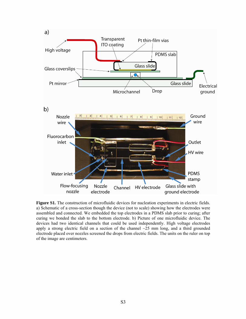
Figure S1. The construction of microfluidic devices for nucleation experiments in electric fields. a) Schematic of a cross-section though the device (not to scale) showing how the electrodes were assembled and connected. We embedded the top electrodes in a PDMS slab prior to curing; after curing we bonded the slab to the bottom electrode. b) Picture of one microfluidic device. The devices had two identical channels that could be used independently. High voltage electrodes apply a strong electric field on a section of the channel ~25 mm long, and a third grounded electrode placed over nozzles screened the drops from electric fields. The units on the ruler on top of the image are centimeters.

S3

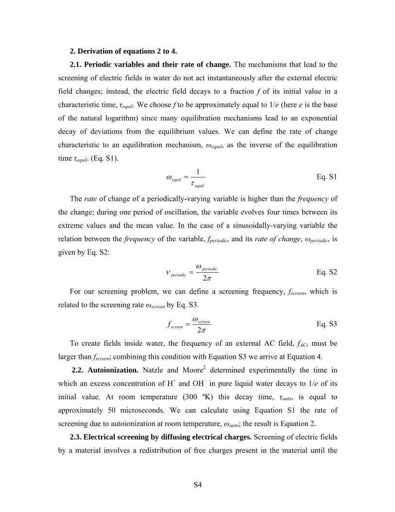
2. Derivation of equations 2 to 4.

2.1. Periodic variables and their rate of change. The mechanisms that lead to the

screening of electric fields in water do not act instantaneously after the external electric

field changes; instead, the electric field decays to a fraction f of its initial value in a

characteristic time, τequil. We choose f to be approximately equal to 1/e (here e is the base

of the natural logarithm) since many equilibration mechanisms lead to an exponential

decay of deviations from the equilibrium values. We can define the rate of change

characteristic to an equilibration mechanism, ωequil, as the inverse of the equilibration

time τequil. (Eq. S1).

equilequil

1 Eq. S1

The rate of change of a periodically-varying variable is higher than the frequency of

the change; during one period of oscillation, the variable evolves four times between its

extreme values and the mean value. In the case of a sinusoidally-varying variable the

relation between the frequency of the variable, fperiodic, and its rate of change, ωperiodic, is

given by Eq. S2:

2periodic

periodic Eq. S2

For our screening problem, we can define a screening frequency, fscreen, which is

related to the screening rate ωscreen by Eq. S3.

2screen

screenf Eq. S3

To create fields inside water, the frequency of an external AC field, fAC, must be

larger than fscreen; combining this condition with Equation S3 we arrive at Equation 4.

2.2. Autoionization. Natzle and Moore2 determined experimentally the time in

which an excess concentration of H+ and OH– in pure liquid water decays to 1/e of its

initial value. At room temperature (300 ºK) this decay time, τauto, is equal to

approximately 50 microseconds. We can calculate using Equation S1 the rate of

screening due to autoionization at room temperature, ωauto; the result is Equation 2.

2.3. Electrical screening by diffusing electrical charges. Screening of electric fields

by a material involves a redistribution of free charges present in the material until the

S4

field generated by these charges creates a screening field that cancels the external field.

To estimate the rate of screening in water, we use a system that is composed of a flat

interface between water and air; an external field that is perpendicular to the interface and

has a magnitude Eexternal is applied instantaneously on the system. The electric field inside

water, Ewater, is initially equal to the field in air, but it is rapidly reduced by a factor equal

to the dielectric constant of water, εw, as water molecules polarize and reorient their

dipole moments in response to the field. This reduction in the field is completed in a time

on the order of a nanosecond, which is much faster than the rate at which our external

fields vary; therefore the field in water is given by Eq. S4:

w

externalwater

EE

Eq. S4

Eventually, magnitude of the electric field in water drops to zero as free H+ and OH–

ions drift due to the field Ewater and build up surface charge at the air/water interface. This

surface charge creates an electric field, EDebye, which opposes Ewater and grows until it

cancels it.

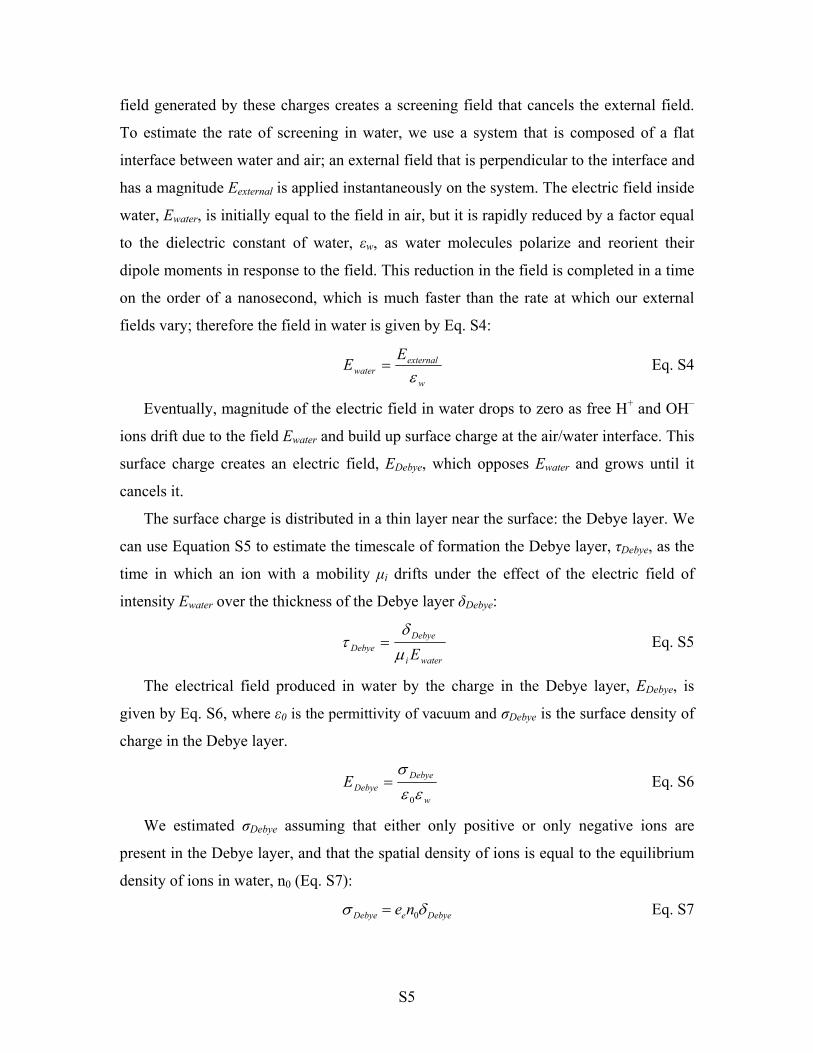
The surface charge is distributed in a thin layer near the surface: the Debye layer. We

can use Equation S5 to estimate the timescale of formation the Debye layer, τDebye, as the

time in which an ion with a mobility μi drifts under the effect of the electric field of

intensity Ewater over the thickness of the Debye layer δDebye:

wateri

DebyeDebye E

Eq. S5

The electrical field produced in water by the charge in the Debye layer, EDebye, is

given by Eq. S6, where ε0 is the permittivity of vacuum and σDebye is the surface density of

charge in the Debye layer.

w

DebyeDebyeE

0

Eq. S6

We estimated σDebye assuming that either only positive or only negative ions are

present in the Debye layer, and that the spatial density of ions is equal to the equilibrium

density of ions in water, n0 (Eq. S7):

DebyeeDebye ne 0 Eq. S7

S5

In Eq. S7, ee is the charge of the electron. Combining Eq. S5 to S7, we deduce a

formula for τDebye (Eq. S8):

ie

wDebye ne

0

0 Eq. S8

Equation 3 follows from Eq. S8 if we define the rate of screening due to charge

diffusion, ωDebye, to be the inverse of the timescale of formation the Debye layer τDebye.

3. The electrical circuit.

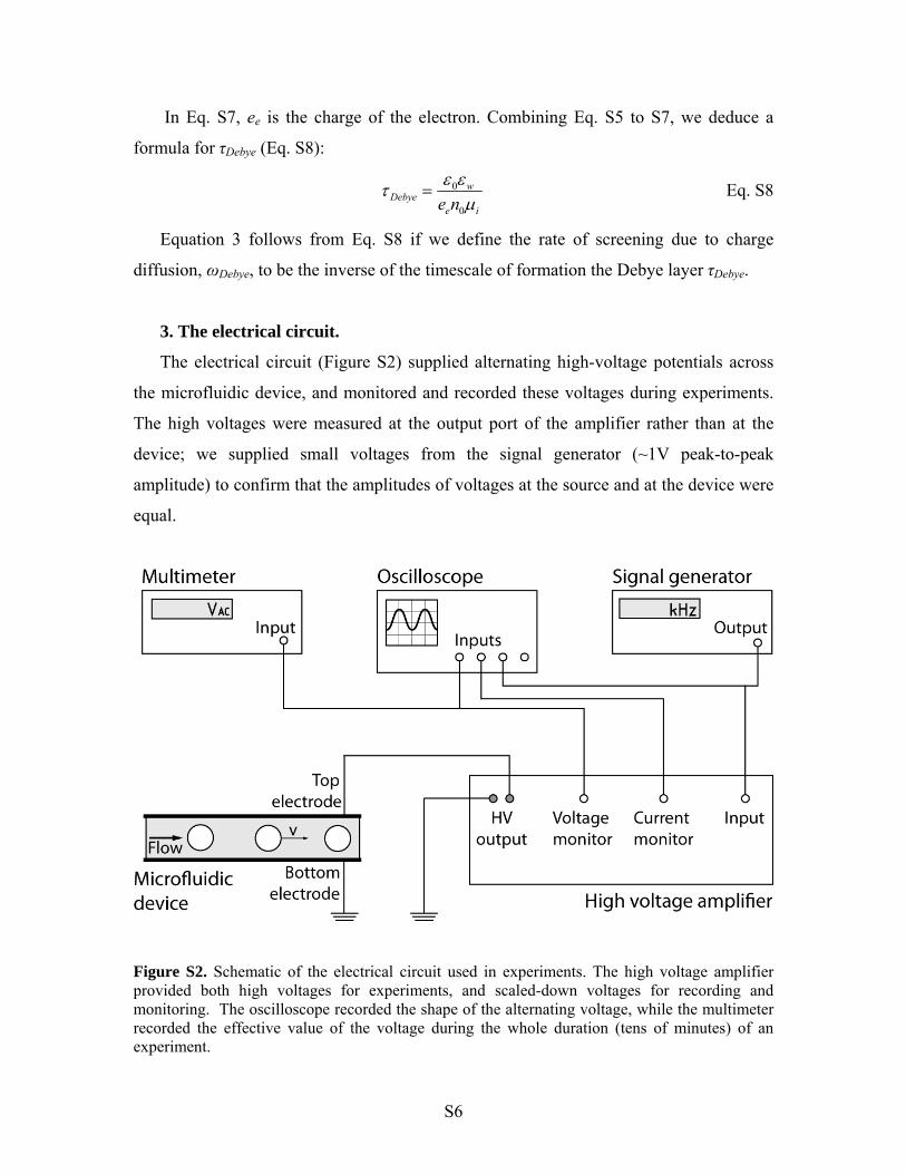
The electrical circuit (Figure S2) supplied alternating high-voltage potentials across

the microfluidic device, and monitored and recorded these voltages during experiments.

The high voltages were measured at the output port of the amplifier rather than at the

device; we supplied small voltages from the signal generator (~1V peak-to-peak

amplitude) to confirm that the amplitudes of voltages at the source and at the device were

equal.

Figure S2. Schematic of the electrical circuit used in experiments. The high voltage amplifier provided both high voltages for experiments, and scaled-down voltages for recording and monitoring. The oscilloscope recorded the shape of the alternating voltage, while the multimeter recorded the effective value of the voltage during the whole duration (tens of minutes) of an experiment.

S6

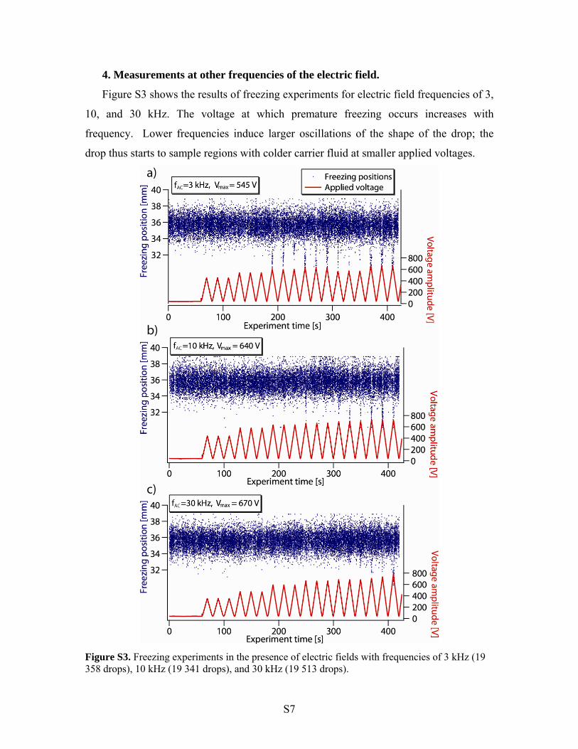
4. Measurements at other frequencies of the electric field.

Figure S3 shows the results of freezing experiments for electric field frequencies of 3,

10, and 30 kHz. The voltage at which premature freezing occurs increases with

frequency. Lower frequencies induce larger oscillations of the shape of the drop; the

drop thus starts to sample regions with colder carrier fluid at smaller applied voltages.

Figure S3. Freezing experiments in the presence of electric fields with frequencies of 3 kHz (19 358 drops), 10 kHz (19 341 drops), and 30 kHz (19 513 drops).

S7

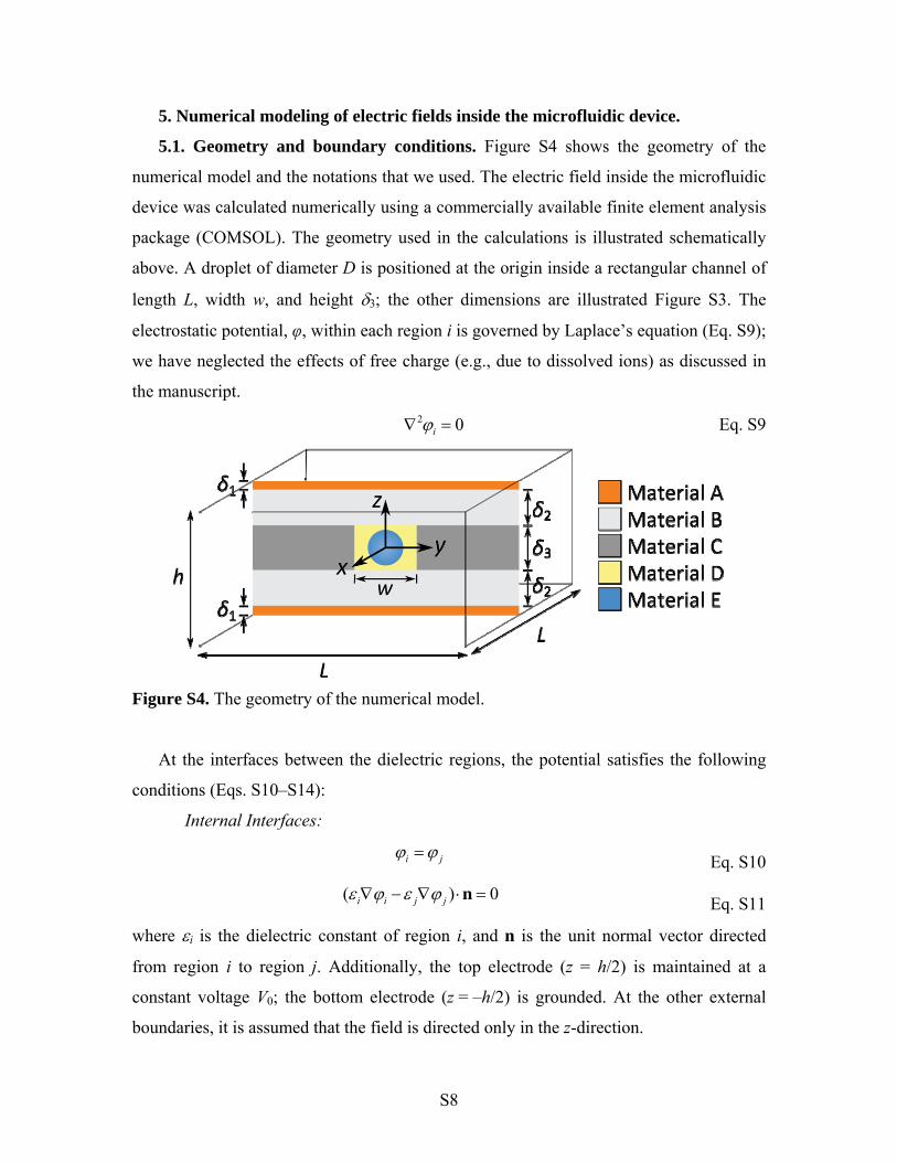
5. Numerical modeling of electric fields inside the microfluidic device.

5.1. Geometry and boundary conditions. Figure S4 shows the geometry of the

numerical model and the notations that we used. The electric field inside the microfluidic

device was calculated numerically using a commercially available finite element analysis

package (COMSOL). The geometry used in the calculations is illustrated schematically

above. A droplet of diameter D is positioned at the origin inside a rectangular channel of

length L, width w, and height 3; the other dimensions are illustrated Figure S3. The

electrostatic potential, φ, within each region i is governed by Laplace’s equation (Eq. S9);

we have neglected the effects of free charge (e.g., due to dissolved ions) as discussed in

the manuscript.

2 0i Eq. S9

Figure S4. The geometry of the numerical model.

At the interfaces between the dielectric regions, the potential satisfies the following

conditions (Eqs. S10–S14):

Internal Interfaces:

i j Eq. S10

( )i i j j 0 n Eq. S11

where i is the dielectric constant of region i, and n is the unit normal vector directed

from region i to region j. Additionally, the top electrode (z = h/2) is maintained at a

constant voltage V0; the bottom electrode (z = –h/2) is grounded. At the other external

boundaries, it is assumed that the field is directed only in the z-direction.

S8

External Boundaries:

0( / 2)z h V Eq. S12

( / 2) 0z h Eq. S13

( ) 0 n at / 2y L and / 2x L Eq. S14

After solving for the electric potential throughout the domain, we compute the average

electric field within the droplet, Edrop, as (Eq. S15):

Eq. S15

drop

drop

V

dV E

Because the field is not perfectly uniform within the drop, we also computed the

variance σdrop,i of each component i of the field about the mean value using Eq. S16:

2

2, ,

drop

drop i drop iiV

E dx

V

Eq. S16

5.2. Numerical results. In this section of the supporting information, we expressed

all electric fields as a fraction of the ‘average’ applied field, E0 = V0 / h. We calculated

the magnitude of the field inside the drops for three cases: (1) using the most probable

values of the experimental parameters; (2) using the limit values of experimental

parameters that correspond to an upper limit of field; and (3) using the limit values of

experimental parameters that correspond to a lower limit of the field. Case 1 corresponds

to the most probable value of the field. Table ST-1 lists the experimental parameters of

case 1 and the corresponding values of the electric field, and Figure S5 shows the

magnitude of electric fields inside the device.

Table ST-1. Case 1: most probable parameter values, and corresponding electric fields. Parameters

1 20 m A (Epoxy) 4 2 150 m B (Glass) 6.7 3 125 m C (PDMS) 2.65 w 200 m D (PFMD) 2.13 D 70m E (water) 110

Results

i = x i = y i = z Edrop,i / E0 0 0 0.110 i / E0 4.0×10–4 3.3×10–4 6.1×10–4

S9

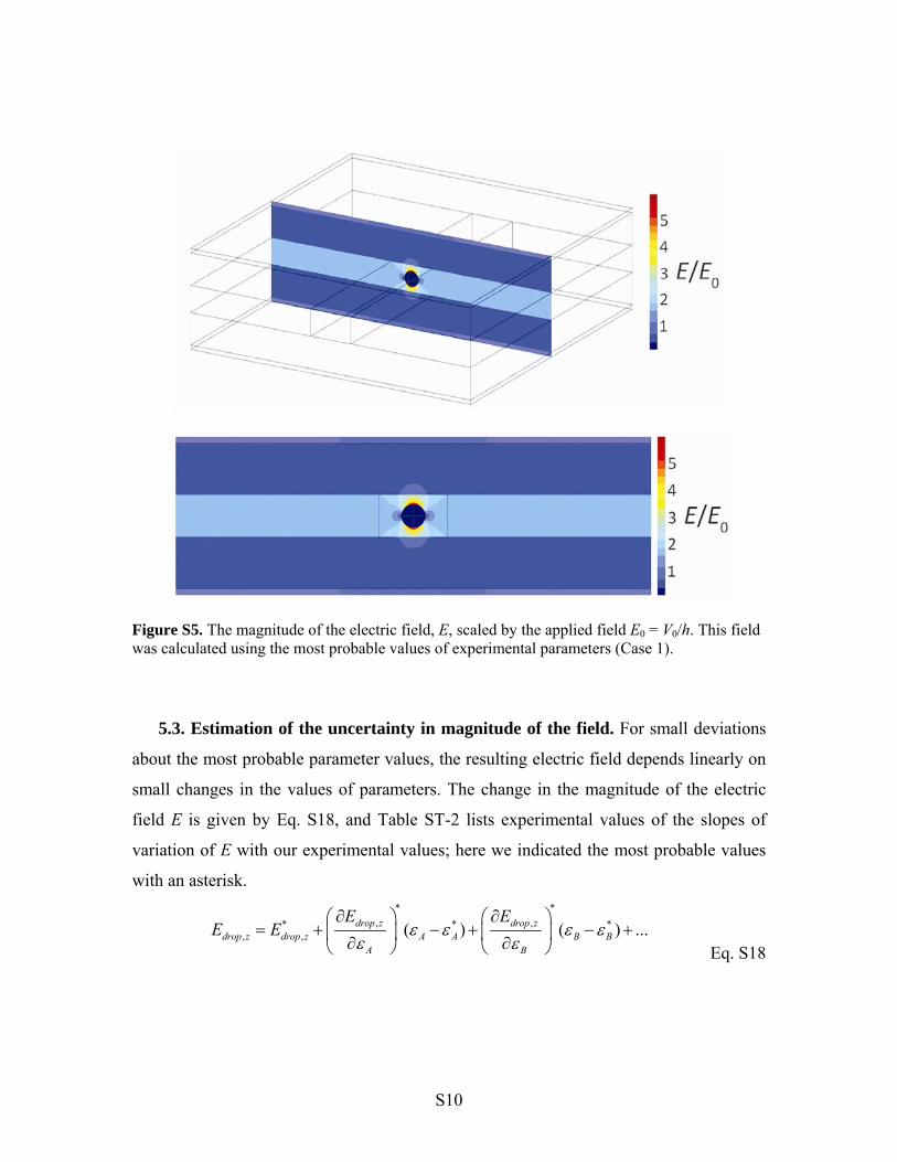
Figure S5. The magnitude of the electric field, E, scaled by the applied field E0 = V0/h. This field was calculated using the most probable values of experimental parameters (Case 1).

5.3. Estimation of the uncertainty in magnitude of the field. For small deviations

about the most probable parameter values, the resulting electric field depends linearly on

small changes in the values of parameters. The change in the magnitude of the electric

field E is given by Eq. S18, and Table ST-2 lists experimental values of the slopes of

variation of E with our experimental values; here we indicated the most probable values

with an asterisk.

* *

, ,* *, , ( ) ( ) ...drop z drop z

drop z drop z A A B BA B

E EE E

*

Eq. S18

S10

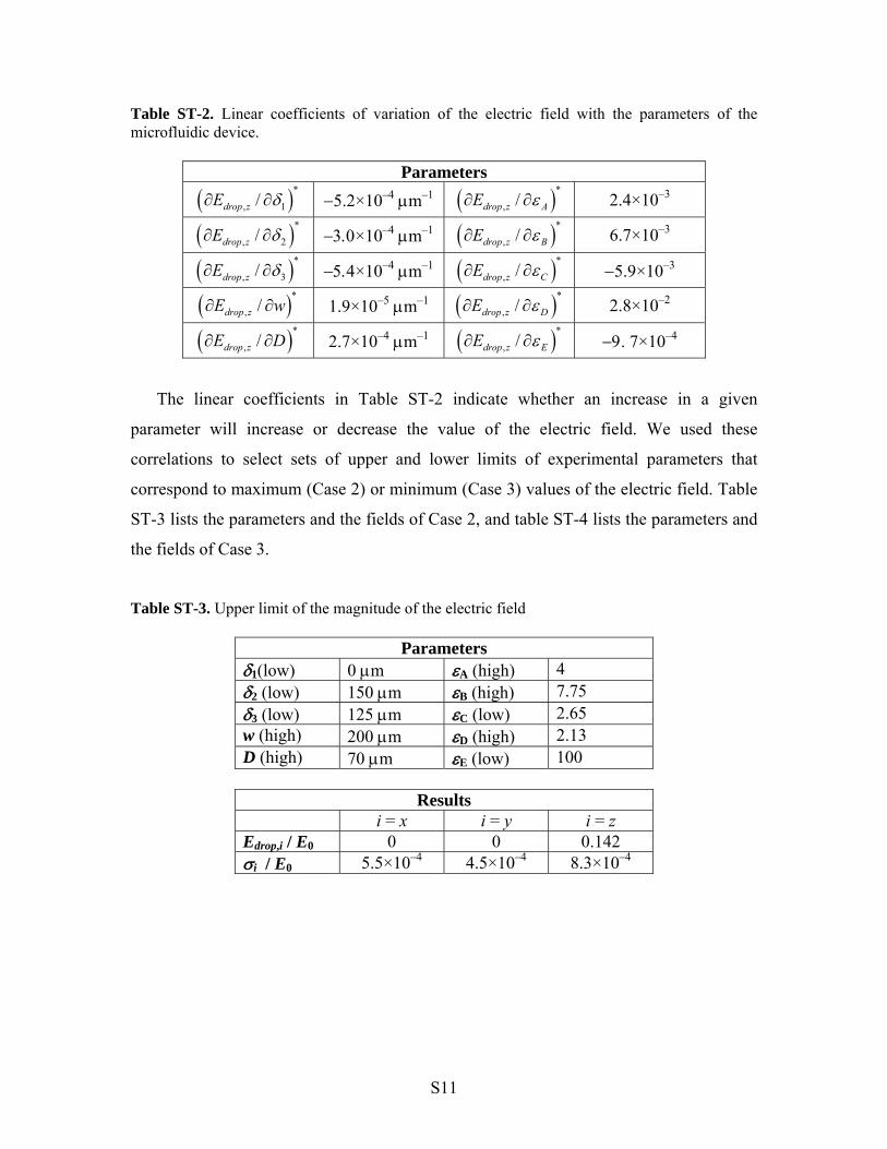
Table ST-2. Linear coefficients of variation of the electric field with the parameters of the microfluidic device.

Parameters

*

, 1/drop zE 5.2×10–4 m–1 *

, /drop z AE 2.4×10–3

*

, 2/drop zE ×10–4 m–1 *

, /drop z BE 6.7×10–3

*

, 3/drop zE ×10–4 m–1 *, /drop z CE 5.9×10–3

*

, /drop z E w 1.9×10–5 m–1 *

, /drop z DE 2.8×10–2

*

, /drop z E D 2.7×10–4 m–1 *, /drop z EE . 7×10–4

The linear coefficients in Table ST-2 indicate whether an increase in a given

parameter will increase or decrease the value of the electric field. We used these

correlations to select sets of upper and lower limits of experimental parameters that

correspond to maximum (Case 2) or minimum (Case 3) values of the electric field. Table

ST-3 lists the parameters and the fields of Case 2, and table ST-4 lists the parameters and

the fields of Case 3.

Table ST-3. Upper limit of the magnitude of the electric field

Parameters 1(low) 0 m A (high) 4 2 (low) 150 m B (high) 7.75 3 (low) 125 m C (low) 2.65 w (high) 200 m D (high) 2.13 D (high) 70m E (low) 100

Results

i = x i = y i = z Edrop,i / E0 0 0 0.142 i / E0 5.5×10–4 4.5×10–4 8.3×10–4

S11

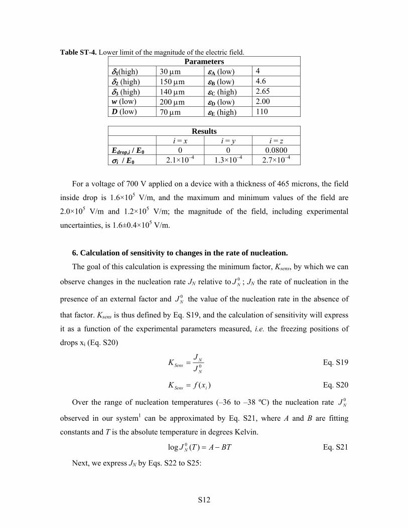
Table ST-4. Lower limit of the magnitude of the electric field. Parameters

1(high) 30 m A (low) 4 2 (high) 150 m B (low) 4.6 3 (high) 140 m C (high) 2.65 w (low) 200 m D (low) 2.00 D (low) 70m E (high) 110

Results

i = x i = y i = z Edrop,i / E0 0 0 0.0800 i / E0 2.1×10–4 1.3×10–4 2.7×10–4

For a voltage of 700 V applied on a device with a thickness of 465 microns, the field

inside drop is 1.6×105 V/m, and the maximum and minimum values of the field are

2.0×105 V/m and 1.2×105 V/m; the magnitude of the field, including experimental

uncertainties, is 1.6±0.4×105 V/m.

6. Calculation of sensitivity to changes in the rate of nucleation.

The goal of this calculation is expressing the minimum factor, Ksens, by which we can

observe changes in the nucleation rate JN relative to ; JN the rate of nucleation in the

presence of an external factor and the value of the nucleation rate in the absence of

that factor. Ksens is thus defined by Eq. S19, and the calculation of sensitivity will express

it as a function of the experimental parameters measured, i.e. the freezing positions of

drops xi (Eq. S20)

0NJ

0NJ

0N

NSens J

JK Eq. S19

)( iSens xfK Eq. S20

Over the range of nucleation temperatures (–36 to –38 ºC) the nucleation rate

observed in our system1 can be approximated by Eq. S21, where A and B are fitting

constants and T is the absolute temperature in degrees Kelvin.

0NJ

BTATJ N )(log 0 Eq. S21

Next, we express JN by Eqs. S22 to S25:

S12

BTAKTJ sensN log)(log Eq. S22

B

KBBTATJ sens

N

log)(log Eq. S23

)(log)()(log 0 TTJTtBATJ NN Eq. S24

Equation S24 shows that within the range of temperatures in which drops nucleate ice

homogenously, an increase in the nucleation rate by a factor Ksens is equivalent to a shift

in the temperatures of nucleation, δT, that is given by Eq. S25:

B

KT senslog Eq. S25

For the nucleation experiments reported here the relation between freezing

temperatures and freezing positions was approximately linear, therefore we expressed the

shift in the temperatures of nucleation, δT, as a function of the minimum observable shift

in freezing positions, δx, the spread of freezing positions, Δx, and the spread of nucleation

temperatures ΔT (Eq. S16):

Tx

xT

Eq. S26

Combining Eq. S25 with Eq. S26, we can then express Ksens as (Eq. S27):

Tx

xB

Ksens

10 Eq. S27

Fitting the rate of homogenous nucleation from Ref. S1 with Eq. S21 we

determined , and we used the spread of temperatures of nucleation from data in

Ref. S1 to get The data shown in Figure 2 has a spread of freezing positions

of To determine δx, we performed first a 100-point running average of the

raw data to determine the approximate average of the freezing positions. We chose the

number of points in the running average such that the intensity of the electric field is

approximately constant during the time required for recording the number of data used in

the running average. Recording 100 points requires 2 seconds of operation – equal to one

tenth of the period of modulation of the electric field. δx was equal to three times the

standard deviation of the running average during one cycle of the modulation of the

1Cº2 B

2T

mm.

C.º

7x

S13

electric field; mm.3.0δ x

Cº

Using these values of B, δx, Δx, and ΔT, Eq. S26

gives , and Eq. 27 gives09.0δ T 1.5.sensK

)(

7. Derivation of Equation 12.

7.1. Model. We will derive Equation 12 using a system of Nw=1000 molecules of

water; this number is approximately equal to the number of molecules in a critical

nucleus of ice during homogeneous nucleation. In our calculations we assumed that the

surface energy between ice XI and supercooled water is the same as the one between ice

Ih and supercooled water. Using this assumption, the difference in free energies is equal

to the difference between the free energies of the bulk of the system.

7.2 The free energy of ferroelectric ice at 235 ºK. The free energy of ice XI is equal

to free energy of ice Ih at the temperature of the ferroelectric ordering transition, TXI-Ih.

We used this equality to estimate the difference between free energies of ices above TXI-Ih.

At TXI-Ih the relation between thermodynamic functions is given by Eq. S28,

0)()( IhXIIh T XIG IhXIIhXIIhIhXI TSH XIIhXI TT Eq. S28

where ΔGXI-Ih(T) is the difference between the free energies of the ferroelectric and

hexagonal ice nuclei, and ΔHXI-Ih and ΔSXI-Ih are the differences between enthalpies, and

between entropies, of the two nuclei. To evaluate ΔGXI-Ih(T), we made the assumption

that ΔHXI-Ih and ΔSXI-Ih do not depend on temperature. This assumption that ΔHXI-Ih does

not depend on temperature is supported by experimental measurements of the specific

heat of ice XI; the difference between the specific heats of ice Ih and ice XI is negligible

below TXI-Ih3. Above TXI-Ih, ΔHXI-Ih is likely to remain constant because it arises from

electrostatic interactions between molecules4; electrostatic interactions in an ice crystal

do not change significantly when the temperature is changed. The value of ΔGXI-Ih(T)

above TXI-Ih is given by Eq. S29, in which we used Eq. S28 to express ΔHXI-Ih as a

function of ΔSXI-Ih.

)()( IhXIIhXIIhXIIhXIIhXI TTSSTHTG Eq. S29

The difference in entropy between the two phases is caused by proton disorder in

hexagonal ice. In hexagonal ice the configurational contribution to entropy per molecule,

s, was calculated theoretically by Pauling5 to be s = kB ln(3/2), where kB is Boltzmann’s

S14

constant. Equation S30 gives the free energy of ferroelectric ice relative to the free

energy of hexagonal ice:

2

3ln)()( IhXIBwIhXI TTkNTG Eq. S30

7.3. Electrostatic contributions to free energy. A particle with a permanent electric

dipole of moment p that has a an absolute temperature T and is placed in an uniform

external field of magnitude E will be influenced by the field such that on average, the

projection of the dipole moment along the direction of the field is .Ep The electrostatic

free energy of the particle is equal to the electrostatic energy of the particle when the

system is in thermodynamic equilibrium at temperature T. The free energy is thus given

by Eq S31:

EparticleE pEG , Eq. S31

The average of the dipole moment, Ep , can be much smaller than p in weak electric

fields because of thermal agitation. We can evaluate the magnitude of a strong electric

field that orients dipoles against thermal agitation, Ep, using Eq. S32:

p

TkE b

p Eq. S32

For a molecule of water in ice Ih (p = pw = 6.2×10–30 C·m) at a temperature that is

typical for homogenous nucleation (T = 235 ºK), for a ferroelectric

nucleus (p ~ Nw pw = 6.2×10–27 C·m), Since the largest fields that

we might investigate experimentally in micron-sized samples of water have magnitudes

between Ep,water and Ep,nucleus, we made the simplifying assumptions that (i) the water

molecules in the nucleus of ice Ih are not aligned along the field, and (ii) the ferroelectric

nucleus, along with all molecules in it, is perfectly aligned with the field. The average

dipole moments,

V/m;105 8, waterpE

V/m.105 5, nucleuspE

IhEp , and XIEp , , of the hexagonal and ferroelectric nuclei are then given

by Eqs. S33 and S34:

0, IhEp Eq. S33

wwXIE pNp , Eq. S34

S15

S16

Equation S35 expresses the difference between the electrostatic free energies of the

two nuclei, ΔGE,XI-Ih, :

wwIhEXIEIhXIE pENppEG ,,, Eq. S35

Adding the electrostatic contribution to the temperature-dependent formula for the

difference of free energies (Eq.S30) we obtain the following formula for the total

difference in free energies (Eq. S36):

wwIhXIBwIhXI pENTTkNTEG

2

3ln)(),( Eq. S36

Equation 12 was derived from Eq. S36 using the condition .0),( nuclferroIhXI TEG

References

(1) Stan, C. A.; Schneider, G. F.; Shevkoplyas, S. S.; Hashimoto, M.; Ibanescu, M.; Wiley, B. J.; Whitesides, G. M. Lab Chip 2009, 9, 2293–2305.

(2) Natzle, W. C.; Moore, C. B. J. Phys. Chem. 1985, 89, 2605–2612.

(3) Tajima, Y.; Matsuo, T.; Suga, H. J. Phys. Chem. Solids 1984, 45, 1135–1144.

(4) Buch, V.; Sandler, P.; Sadlej, J. J. Phys. Chem. B 1998, 102, 8641–8653.

(5) Pauling, L. J. Am. Chem. Soc. 1935, 57, 2680–2684.