strongly non-linear stochastic response of a system with random initial imperfections
TRANSCRIPT

Strongly non-linear stochastic response of a system with random initialimperfections
J. NaÂprstek
Institute of Theoretical and Applied Mechanics, Prosecka 76, 190 00 Prague 9, Czech Republic
Abstract
Strongly non-linear responses of structures with random imperfections of Gaussian type in their geometrical form under slowly increasing
loading are investigated. Large displacements as a source of non-linearities are taken into account. Imperfections are considered as stochastic
functions of space coordinates. The ®nite element method is supposed as a basis. A stochastic version of the arc length method of stochastic
non-linear algebraic systems in linearised formulation is proposed. A closed interaction between deterministic and stochastic parts of
response is demonstrated. Several numerical tests of theoretical results on simple Mieses frames modelling imperfect shallow shells have
been carried out. Analytical and numerical results make it possible to demonstrate non-conventional properties typical for a randomly
imperfect structure with a tendency to various types of snap-through effects. q 1998 Elsevier Science Ltd. All rights reserved.
1. Introduction
There are various descriptions of the loss of stability so as
to comply with a particular ®eld of research and sometimes
even with particular problems. However, all these de®ni-
tions concern a situation in which the combination of the
parameters describing the system and the parameters
describing its excitation results in the loss of correctness
of the problem.
In the ®eld of thin-walled structures exposed to static
loads the state of equilibrium may have several forms
which in themselves may be stable or unstable. The transi-
tion between them will proceed spontaneously or by snap
through a very low energy barrier. Such a process may be
entirely local and insigni®cant for the system as a whole
which can be exposed to further loads or it may mean its
partial or entire collapse.
We shall deal with the problem of a strongly non-linear
response of a thin-walled system subjected to a load slowly
increasing so that it can be considered static in every step.
The non-linearity is understood in the meaning of major
displacements, i.e. as a non-linear relation between displa-
cements and deformation. The constitutive relations are
considered linear, the forces of inertia neglected.
When solving the so-formulated problem by the ®nite
element method in the deterministic formulation, we arrive
at the problem of solving a non-linear algebraic equation
system:
f�r;u;l� � 0 (1)
where r is a vector of internal parameters of the system
(description of geometry, physical characteristics, etc.), m
elements; u is a vector of displacements of grid nodes, n
elements; and l is a load parameter.
The system in Eq. (1) contains unknown components of
vector u in the ®rst to third powers in the form of a sum of
homogeneous functions (in Euler's meaning) of correspond-
ing orders [1±3]. We assume that the functions fi(i� 1,¼,n)
are continuous and suf®ciently smooth.
The solution of the system in Eq. (1) by the incremental
method with predetermined loading steps Dl [4, 5], fails in
the vicinity of the extreme of any curve ui(l ) and in the
vicinity of the bifurcation point. After numerous attempts,
the solution of which could be applied to a limited region
only, a more universal method was ®nally found [6, 7]
which was called the `arc length method'. It is based on
the fact that it does not increment l , or any component of
u, but the length of the arc of the response curve. The given
quantity, therefore, is the length of the vector uDut,Dl uwhich is assumed not to differ much from the actual length
of the arc as a curve in n-dimensional space. The increment
of the loading parameter, consequently, is one of the
unknown quantities and not the given quantity.
The whole process can be interpreted geometrically as
shown in Fig. 1. We start from the initial point M of one
step. In the ®rst phase in the direction of the tangent to the
curve in the point M we arrive at the point N0 which is
situated outside the response curve and does not comply,
consequently, with the system in Eq. (1). In the second
phase the classical incremental method makes use of
Probabilistic Engineering Mechanics 14 (1999) 141±148
0266-8920/99/$ - see front matter q 1998 Elsevier Science Ltd. All rights reserved.
PII: S0266-8920(98)00024-1
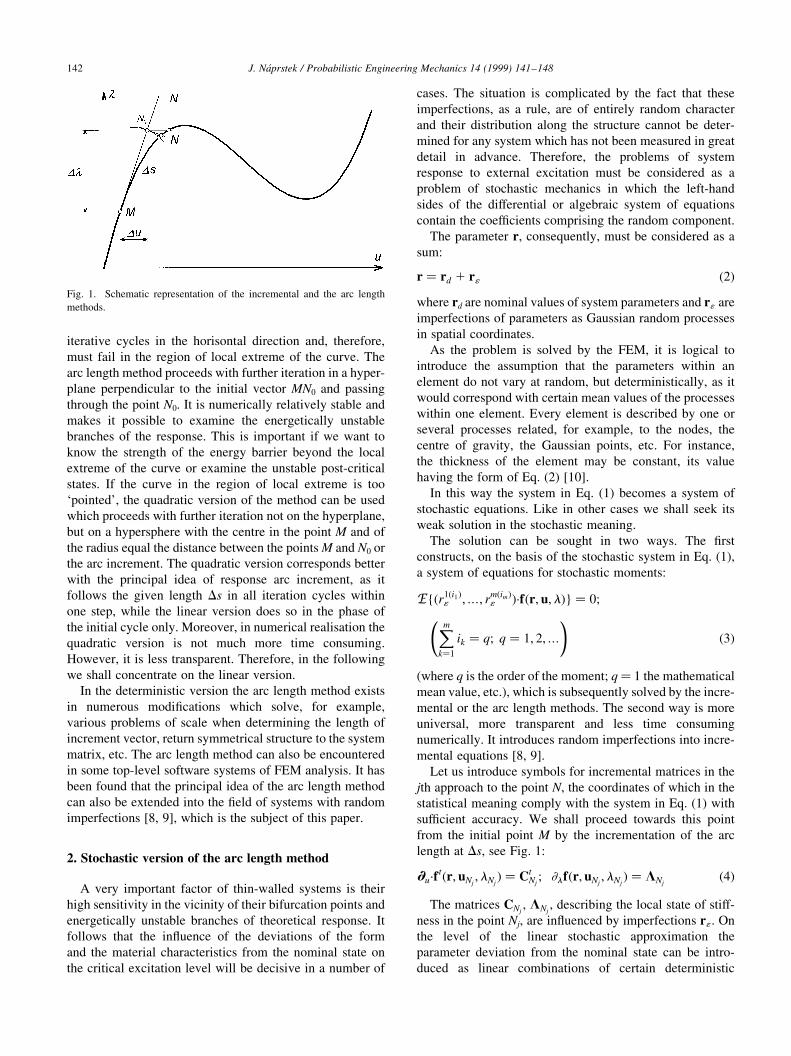
iterative cycles in the horisontal direction and, therefore,
must fail in the region of local extreme of the curve. The
arc length method proceeds with further iteration in a hyper-
plane perpendicular to the initial vector MN0 and passing
through the point N0. It is numerically relatively stable and
makes it possible to examine the energetically unstable
branches of the response. This is important if we want to
know the strength of the energy barrier beyond the local
extreme of the curve or examine the unstable post-critical
states. If the curve in the region of local extreme is too
`pointed', the quadratic version of the method can be used
which proceeds with further iteration not on the hyperplane,
but on a hypersphere with the centre in the point M and of
the radius equal the distance between the points M and N0 or
the arc increment. The quadratic version corresponds better
with the principal idea of response arc increment, as it
follows the given length Ds in all iteration cycles within
one step, while the linear version does so in the phase of
the initial cycle only. Moreover, in numerical realisation the
quadratic version is not much more time consuming.
However, it is less transparent. Therefore, in the following
we shall concentrate on the linear version.
In the deterministic version the arc length method exists
in numerous modi®cations which solve, for example,
various problems of scale when determining the length of
increment vector, return symmetrical structure to the system
matrix, etc. The arc length method can also be encountered
in some top-level software systems of FEM analysis. It has
been found that the principal idea of the arc length method
can also be extended into the ®eld of systems with random
imperfections [8, 9], which is the subject of this paper.
2. Stochastic version of the arc length method
A very important factor of thin-walled systems is their
high sensitivity in the vicinity of their bifurcation points and
energetically unstable branches of theoretical response. It
follows that the in¯uence of the deviations of the form
and the material characteristics from the nominal state on
the critical excitation level will be decisive in a number of
cases. The situation is complicated by the fact that these
imperfections, as a rule, are of entirely random character
and their distribution along the structure cannot be deter-
mined for any system which has not been measured in great
detail in advance. Therefore, the problems of system
response to external excitation must be considered as a
problem of stochastic mechanics in which the left-hand
sides of the differential or algebraic system of equations
contain the coef®cients comprising the random component.
The parameter r, consequently, must be considered as a
sum:
r � rd 1 r1 (2)
where rd are nominal values of system parameters and r1 are
imperfections of parameters as Gaussian random processes
in spatial coordinates.
As the problem is solved by the FEM, it is logical to
introduce the assumption that the parameters within an
element do not vary at random, but deterministically, as it
would correspond with certain mean values of the processes
within one element. Every element is described by one or
several processes related, for example, to the nodes, the
centre of gravity, the Gaussian points, etc. For instance,
the thickness of the element may be constant, its value
having the form of Eq. (2) [10].
In this way the system in Eq. (1) becomes a system of
stochastic equations. Like in other cases we shall seek its
weak solution in the stochastic meaning.
The solution can be sought in two ways. The ®rst
constructs, on the basis of the stochastic system in Eq. (1),
a system of equations for stochastic moments:
E{�r1�i1�1 ;¼; rm�im�
1 �´f�r; u;l�} � 0;
Xmk�1
ik � q; q � 1; 2;¼
!(3)
(where q is the order of the moment; q� 1 the mathematical
mean value, etc.), which is subsequently solved by the incre-
mental or the arc length methods. The second way is more
universal, more transparent and less time consuming
numerically. It introduces random imperfections into incre-
mental equations [8, 9].
Let us introduce symbols for incremental matrices in the
jth approach to the point N, the coordinates of which in the
statistical meaning comply with the system in Eq. (1) with
suf®cient accuracy. We shall proceed towards this point
from the initial point M by the incrementation of the arc
length at Ds, see Fig. 1:
2u´f t�r; uNj; lNj� � Ct
Nj; 2lf�r;uNj
;lNj� � LNj
(4)
The matrices CNj, LNj
, describing the local state of stiff-
ness in the point Nj, are in¯uenced by imperfections r1 . On
the level of the linear stochastic approximation the
parameter deviation from the nominal state can be intro-
duced as linear combinations of certain deterministic
J. NaÂprstek / Probabilistic Engineering Mechanics 14 (1999) 141±148142
Fig. 1. Schematic representation of the incremental and the arc length
methods.

shape functions, where the coef®cients of their linear combi-
nations are random processes. The shape functions may
consist of the system of `pyramids' with the vertices in
the individual network nodes, the coef®cients of Fourier
series of shell geometric imperfections, etc. In this way
the imperfections are modelled as m of random scalar
processes entering Eq. (1) or Eq. (2). That means that the
local stiffness matrices in Eq. (4) can be written in the form
of:
CNj� C0
Nj1Xmi�1
CiNj
ri1; LNj
� L0Nj
1Xmi�1
LiNj
ri1 (5)
where C0Nj
, L0Nj
are local stiffness matrices in the point Nj of
the system in nominal state; CiNj
, LiNj
are increments of the
matrices C0Nj
, L0Nj
due to `unit' imperfection; and ri1 is the
value of the ith imperfection (Gaussian random centred
processes).
The increments of displacement and load will be
expressed in similar form, i.e. as linear combinations of
certain generalised coordinates (or unknown shape func-
tions), where the coef®cients of these combinations are the
same random processes ri1 as in the case of Eq. (5):
DuNj� Du0
Nj1Xmi�1
DuiNj
ri1; DlNj
� Dl0Nj
1Xmi�1
DliNj
ri1 (6)
The adopted level of local linear stochastic approxima-
tion of stiffness Eq. (5) corresponds with the Gaussian
stochastic part of the response within one iteration cycle.
The solution of the response of an imperfect system, once
again, is based on the incremental form of the system in Eq.
(1) in homogeneous form, supplemented with the constraint
of the constant arc length Ds. This means that the load
increment is not known, i.e. is one of the unknown quanti-
ties, in the same way as all displacement increments in the
nodes. If we are to proceed from the point M to the point N
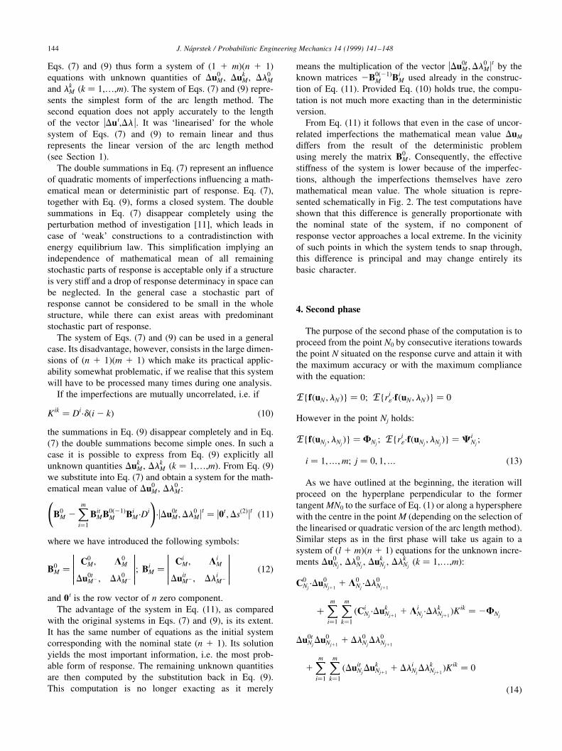
on the response hyperplane, we shall proceed in two phases,
see Fig. 2.
3. First phase
In the ®rst phase we shall proceed tangentially to the
point N0. This will be achieved by the solution of a linear
system which will originate as follows: the incrementation
of Eq. (1) in the point M; the subsequent substitution accord-
ing to Eqs. (4)±(6) (Nj should be replaced by M) and the
application of the operator of the mathematical mean value
1{´} in the Gaussian meaning. We obtain in such a way the
®rst part of the system describing the mathematical mean
value and the generalised coordinates of the stochastic part
of the response in the ®rst phase; this means moving from
the point M to the point N0:
C0M´Du0
M 1 L0M´Dl0
M
1Xmi�1
Xmk�1
�CiM´Duk
M 1 LiM´Dlk
M�´Kik � 0
Du0tM2 ´Du0
m 1 Dl0M2 ´Dl0
M
1Xmi�1
Xmk�1
�DuitM2 ´Duk
M 1 DliM2 ´Dlk
M�´Kik � Ds�2�
(7)
using the validity of the following relations:
E{ri1´r
i1k} � Kik; E{ri
1} � 0 (8)
In Eq. (7) Du0tM2 , Duit
M2 , Dl0M2 and Dli
M2 should be under-
stood as total increments in a preceding step which has been
®nished in the point M. In the very beginning a solution of a
corresponding linear problem can be used.
The system of Eq. (7) represents a system of n 1 1 equa-
tions for (1 1 m)(n 1 1) unknown increment values Du0M ,
DukM , Dl0
M and lkm. The remaining equations can be obtained
by the multiplication of the system in Eq. (1) before the
application of the operator E{´} to this incremental system
and to the constraint of the constant arc length by the
process rl1. In this way a similar procedure for l � 1,¼,m
will produce m systems of n 1 1 equations each:Xmi�1
�CiM´Du0
M 1 LiM´Dl0
M�Kli
1Xmk�1
�C0M´Duk
M 1 L0M´Dlk
M�´Klk � 0
Xmi�1
�DuitM2 ´Du0
m 1 DliM2 ´Dl0
M�Kli
1Xmk�1
�Du0tM2 ´Duk
M 1 Dl0M2 ´Dlk
M�´Klk � 0
(9)
J. NaÂprstek / Probabilistic Engineering Mechanics 14 (1999) 141±148 143
Fig. 2. Schematic representation of the arc length method in stochastic
version.
Eqs. (7) and (9) thus form a system of (1 1 m)(n 1 1)
equations with unknown quantities of Du0M , Duk
M , Dl0M
and lkM (k � 1,¼,m). The system of Eqs. (7) and (9) repre-
sents the simplest form of the arc length method. The
second equation does not apply accurately to the length
of the vector uDut,Dl u. It was `linearised' for the whole
system of Eqs. (7) and (9) to remain linear and thus
represents the linear version of the arc length method
(see Section 1).
The double summations in Eq. (7) represent an in¯uence
of quadratic moments of imperfections in¯uencing a math-
ematical mean or deterministic part of response. Eq. (7),
together with Eq. (9), forms a closed system. The double
summations in Eq. (7) disappear completely using the
perturbation method of investigation [11], which leads in
case of `weak' constructions to a contradistinction with
energy equilibrium law. This simpli®cation implying an
independence of mathematical mean of all remaining
stochastic parts of response is acceptable only if a structure
is very stiff and a drop of response determinacy in space can
be neglected. In the general case a stochastic part of
response cannot be considered to be small in the whole
structure, while there can exist areas with predominant
stochastic part of response.
The system of Eqs. (7) and (9) can be used in a general
case. Its disadvantage, however, consists in the large dimen-
sions of (n 1 1)(m 1 1) which make its practical applic-
ability somewhat problematic, if we realise that this system
will have to be processed many times during one analysis.
If the imperfections are mutually uncorrelated, i.e. if
Kik � Di´d�i 2 k� (10)
the summations in Eq. (9) disappear completely and in Eq.
(7) the double summations become simple ones. In such a
case it is possible to express from Eq. (9) explicitly all
unknown quantities DukM , Dlk
M (k � 1,¼,m). From Eq. (9)
we substitute into Eq. (7) and obtain a system for the math-
ematical mean value of Du0M , Dl0
M:
B0M 2
Xmi�1
BitMB0�21�
M BiM´Di
!´uDu0t
M ;Dl0M ut � u0t
;Ds�2�ut (11)
where we have introduced the following symbols:
B0M �
C0M ; L0
M
Du0tM2 ; Dl0
M2
������������; Bi
M �Ci
M ; LiM
DuitM2 ; Dli
M2
������������ (12)
and 0t is the row vector of n zero component.
The advantage of the system in Eq. (11), as compared
with the original systems in Eqs. (7) and (9), is its extent.
It has the same number of equations as the initial system
corresponding with the nominal state (n 1 1). Its solution
yields the most important information, i.e. the most prob-
able form of response. The remaining unknown quantities
are then computed by the substitution back in Eq. (9).
This computation is no longer exacting as it merely
means the multiplication of the vector uDu0tM ;Dl
0M ut by the
known matrices 2B0�21�M Bi
M used already in the construc-
tion of Eq. (11). Provided Eq. (10) holds true, the compu-
tation is not much more exacting than in the deterministic
version.
From Eq. (11) it follows that even in the case of uncor-
related imperfections the mathematical mean value DuM
differs from the result of the deterministic problem
using merely the matrix B0M . Consequently, the effective
stiffness of the system is lower because of the imperfec-
tions, although the imperfections themselves have zero
mathematical mean value. The whole situation is repre-
sented schematically in Fig. 2. The test computations have
shown that this difference is generally proportionate with
the nominal state of the system, if no component of
response vector approaches a local extreme. In the vicinity
of such points in which the system tends to snap through,
this difference is principal and may change entirely its
basic character.
4. Second phase
The purpose of the second phase of the computation is to
proceed from the point N0 by consecutive iterations towards
the point N situated on the response curve and attain it with
the maximum accuracy or with the maximum compliance
with the equation:
E{f�uN ;lN�} � 0; E{ri1´f�uN ; lN�} � 0
However in the point Nj holds:
E{f�uNj;lNj�} � FNj
; E{ri1´f�uNj
;lNj�} �Ci
Nj;
i � 1;¼;m; j � 0; 1;¼ (13)
As we have outlined at the beginning, the iteration will
proceed on the hyperplane perpendicular to the former
tangent MN0 to the surface of Eq. (1) or along a hypersphere
with the centre in the point M (depending on the selection of
the linearised or quadratic version of the arc length method).
Similar steps as in the ®rst phase will take us again to a
system of (l 1 m)(n 1 1) equations for the unknown incre-
ments Du0Nj
, Dl0Nj
, DukNj
, DlkNj
(k � 1,¼,m):
C0Nj
´Du0Nj11
1 L0Nj
´Dl0Nj11
�Xmi�1
Xmk�1
�CiNj
´DukNj11
1 LiNj
´DlkNj11�Kik � 2FNj
Du0tNjDu0
Nj111 Dl0
NjDl0
Nj11
1Xmi�1
Xmk�1
�DuitNjDuk
Nj111 Dli
NjDlk
Nj11�Kik � 0
(14)
J. NaÂprstek / Probabilistic Engineering Mechanics 14 (1999) 141±148144

Xmi�1
�CiNjDu0
Nj111 Li
NjDl0
Nj11�Kli
�Xmk�1
�C0NjDuk
Nj111 L0
NjDlk
Nj11�Klk
� 2ClNj
Xmi�1
�DuitNjDu0
Nj111 Dli
NjDl0
Nj11�Kli
1Xmk�1
�Du0tNjDuk
Nj111 Dl0
NjDlk
Nj11�Klk � 0 (15)
The system of Eqs. (14) and (15) is similar to the system of
Eqs. (7) and (9) used in the ®rst phase. Instead of matrices
C0M , L0
M , CiM , Li
M the system makes use of the matrices C0Nj
,
L0Nj
, CiNj
, LiNj
, which correspond with local matrices in the
respective point Nj respecting the result of the preceding
iteration. The right-hand sides of Eqs. (14) and (15) are
replaced with the vectors u 2 FtNj; 0ut and u 2 Clt
Nj; 0ut. The
vectors 2FtNj
, 2CltNj
represent the `error' resulting from the
substitution of Nj in Eq. (3), and the zeros in the last equa-
tions mean the zero increment of the arc which was intro-
duced with its full length in the ®rst phase of the
computation. The system of Eqs. (14) and (15) can be
simpli®ed similarly as the system of Eqs. (7) and (9) in
the case of stochastic independence of imperfections in
space, i.e. if Eq. (10) holds true.
The whole process, i.e. the substitution of DuNj, DlNj
in
Eq. (13), the construction of the system of Eqs. (14) and (15)
for the point Nj, the solution of the system and the determi-
nation of the new point Nj11 is repeated m times, until the
vector norm
uDu0Nj;Dl0
Nj;Du1
Nj;Dl1
Nj;¼;Dum
Nj;Dlm
Nju , 1 (16)
drops below the preset value 1 . In such a case the Nm point
can be stated to be the point N sought in the stochastic
meaning, while m 1 1 will be the number of cycles required
in accordance with Eqs. (13)±(16). When condition (16) is
satis®ed, we can start the next step. Starting this one the Nm
point becomes N an initial point M and the whole process
should be repeated from Eqs. (7) and (9).
On the basis of these computations it is possible to
describe the history of the response of the system in the
course of one step from the point M to the point N as
follows:
uN � uM 1Xmj�0
Du0Nj
1Xmi�1
DuiNj
ri1
!(17)
Hence the mathematical mean value:
E{uN} � uM 1Xmj�0
Du0Nj
(18)
and the mutual correlation of reponse vector component:
E{uN´utN} 2 E{uN}´{ut
N} �Xmk�0
Xmj�0
Xmi�1
Xml�1
DuiNjDult
Nk´Kil
!(19)
Eqs. (18) and (19) make it possible to trace the curves of the
most probable response (mathematical mean value) and
the respective variance zone suggesting how it is
necessary to reduce the critical load level due to introduced
imperfections.
5. Numerical investigations
Several numerical tests on simple Mieses frames model-
ling shallow shells showing strongly non-linear behaviour
have been carried out. Only geometrical uncertainties in the
form have been taken into account. The results of these
computations can be summarised as shown in Fig. 3.
Every point on the curve of the mathematical mean value
of response has a certain corresponding curve showing the
distribution of the probability density of deviations of
displacements in the individual nodes or degrees of freedom
from the mathematical mean value. Hence the upper and
lower boundaries of the region surrounding the curve of
J. NaÂprstek / Probabilistic Engineering Mechanics 14 (1999) 141±148 145
Fig. 3. Mathematical mean value of response and reliability zone.
Fig. 4. Extinction of energy barrier against snap through due to random
imperfections.

the most probable response on both sides. This region can be
called the reliability zone.
For the given probability and the given imperfections
statistics the response of the system will not proceed beyond
this zone. With regard to the manner of origin of the upper
and lower boundary curves, they may be of considerably
complex character, shown in Fig. 3. This means that some
of their parts may not be applied at all in the meaning of
their initial purpose. Both curves may have transition points
and a number of special characteristics. Their evaluation,
therefore, must use the methods related to the speci®c char-
acteristics of their differential geometry.
Fig. 4 shows, on the basis of control computations, the
state in which the imperfections lead to a practical extinc-
tion of the energy barrier preventing the snap through. The
mathematical mean value of the response still has a certain
real part which is energetically unstable and, geometrically,
has a small barrier different from zero. The deviation from
this curve towards lower values, however, leads to a lower
limit curve which is a monotonous function within the deci-
sive interval of the loading process. As it is the lower limit,
below which the response will not drop with the prescribed
probability, it is necessary to respect this curve when asses-
sing the system resistance to buckling and compromise on a
much lower bearing capacity than that ascertained on the
basis of the nominal state.
When analysing these results, let us note also that because
of the lower effective stiffness of the system especially in
the vicinity of the local extreme of the response curve also
the energy barrier, considered merely from the viewpoint of
the mathematical mean value response, will also drop.
Therefore, it is necessary to take into account that the
extinction of the energy barrier may occur even on the
level of the most probable form of response and not only
on the level of the lower reliability boundary.
It can be observed that the reliability zone is much
broader in the region of the local extreme of the mathema-
tical mean value than anywhere else. Consequently, the
system is most highly sensitive to imperfections in the
very places of the possible snap through. This is testi®ed
to also by the markedly higher variance of experimental
results in these very regions.
Particular attention in this respect must be afforded to
bifurcation points. With regard to the stochastic character
of the problem, their position also has a stochastic character.
For the same reason some of them may disappear and others
appear with a certain probability which depends on the
energy gradient in their vicinity.
It must be realised that the response of the system as a
whole with regard to strong non-linearity is markedly non-
Gaussian. Moreover, the original operator is non-convex in
a broad region and it is in this very region that we usually
require most information on system behaviour. On the other
hand it is necessary to realise that this operator acquires in
most of these regions again the convex operator properties
because of the additional constraint ®xing the length of arc
increment. Every step of the solution always proceeds
within a relatively small interval of arc increment where
the system behaviour approaches linear behaviour. For
these reasons the response within every iteration cycle can
be considered approximately Gaussian, even though in the
end the results composed of individual partial steps are of
non-Gaussian character. This effect manifests ®nally on a
level of approach adopted as non-symmetry of the reliability
zone.
Let us show now these effects on two examples of imper-
fect thin-walled shell response. Let us assume that the mate-
rial characteristics (E,n ) and the wall thickness t are
constant without any deviations from the nominal state. In
both cases the shape of the middle plane is burdened with
random imperfections. Its deviations from the nominal state
are introduced in a direction of the normal as the deviation/
wall thickness ratio.
The ®rst case concerns a shallow spherical shell fully
clamped along its boundary and loaded by a uniformly
distributed radial load acting towards the centre of the sphe-
rical surface. We shall introduce the load in the dimension-
less form l � @ 4q/Et4, where @ is the radius of the sperical
J. NaÂprstek / Probabilistic Engineering Mechanics 14 (1999) 141±148146
Fig. 5. Response of a uniformly loaded shallow spherical shell with random imperfections of shape for various rise values.

cap in plan and t the shell thickness (see Fig. 5), E the
Young's modulus of elasticity and q the load in a usual
meaning. The response in Fig. 5 is understood as the ratio
of the maximum displacement in the normal direction and
wall thickness (wmax/t) (in the given case this maximum was
attained always on the top of the sperical cap). Three rise
values of this cap were investigated (V/t � 0,2,4). The ®rst
of them concerns a circular membrane. The random shape
imperfections were considered as a centred homogeneous
Gaussian process with root mean square of s 0 � 1 which
means that the middle plane deviations from the nominal
shape are of the order of one shell wall thickness.
The actual computation was made by the FEM using
quadrilateral shell elements (24 DOE). Using the algoritm
described in previous sections, the second phase of every
step represented 3±16 iterations to achieve displacement
accuracy being better than 1023t in the meaning of mathe-
matical mean value of the response. The results shown in
Fig. 5 reveal that in the ®rst loading phase the same displa-
cement is achieved on the nominal structure (thick dashed
line) under markedly higher load than that corresponding to
the mathematical mean value of the response of the imper-
fect system (thick solid line). This is in accordance with the
general conclusion following directly from Eq. (11) and
illustrated in Fig. 2. In the next phase, on the other hand,
when the system attains stable equilibrium again (after a
snap through), the effective stiffness of the imperfect system
is somewhat higher. In the case of the membrane (V/t � 0)
these phenomena are relatively weak. Although even in this
case the stiffness ratio of the imperfect and nominal system
differs, the differences are almost negligible and are situated
entirely within the reliability zone. On the other hand, in the
case of a rise (V/t $ 2) the differences are considerable. The
imperfect system shows already an energy barrier, while the
mathematical mean value of the response shows none or
only an imperceptible one. Similar tendencies can be
observed in the reliability zone marked with thin solid
lines in Fig. 5. This zone is asymmetrical which manifests
itself particularly in the areas of equilibrium jumps. In the
case of the membrane this asymmetry is negligible. For the
load beyond the buckling limit, it is possible to observe the
tendency that the zone width decreases slightly with the
increasing load and that the mathematical mean value of
the response approaches the response of the nominal struc-
ture. This is valid only until another zone of instability (or
snap through) is achieved. However, the validity of these
results should not be overestimated. They apply only to the
analysed spherical shallow shell and the type of imperfec-
tions concerned.
The second case is a closed thin-walled cylindrical shell
of radius R and length L (L/R� 2, R/t� 100), fully clamped
on both ends. The radial uniformly ditributed load is intro-
duced in the dimensionless form of l� R3q/Et3. The imper-
fections are modelled in the same way as in the case of the
spherical shell. Fig. 6 shows the mathematical mean value
of the response for various imperfection levels of the middle
plane shape (thick solid lines), compared with the response
of the structure in the nominal state (thick dashed line). The
imperfection level is characterised by the values s 0 �1,2,3,4. The computational methodology is the same as in
the preceding case.
Fig. 6 reveals that the difference of the response of the
nominal system and the mathematical mean value (effective
response) of the imperfect system increases with increasing
imperfections level, although the shape imperfections are
described by a centred process. The energy barrier in the
meaning of the mean value disappears when the imperfec-
tions attain the values between s 0 � 2 and 3. The effective
stiffness after a snap through, if there is any, is on a limited
interval higher than this one corresponding with the nominal
shape of the shell.
6. Conclusions
Results of analytical as well as numerical investigations
make it possible to arrive at some qualitative conclusions.
The effective stiffness of an imperfect system in individual
J. NaÂprstek / Probabilistic Engineering Mechanics 14 (1999) 141±148 147
Fig. 6. Response of a uniformly loaded closed cylindrical shell of ®nite length (L/R � 2) for various levels of shape imperfections.

steps is lower than the stiffness of the system with determi-
nistic nominal characteristics until the snap through occurs.
This holds especially in the places of largest imperfections,
and in spite of the fact that the processes describing the
imperfections are centred. The determinism of the response,
which is given by its mathematical mean, decreases with the
distance from the places which are de®ned fully determinis-
tically, e.g. deterministic boundary conditions. The stochas-
tic component of the response increases in a corresponding
manner. Thus in distant parts of the structure the response
can be burdened with a substantial amount of uncertainty.
Numerical calculations performed have revealed that during
the loading process the variance of the response increases
more or less proportionally with its mathematical mean. The
variance starts increasing substantially if the mathematical
mean of the response approaches its local extreme and the
structure tends to the snap through state.
It has been con®rmed once more that the in¯uence of
large and medium imperfections on various types of critical
loading can be introduced by means of convex analysis.
Results obtained by means of stochastic analysis are only
slightly more favourable. However, in the case of small
imperfections, which are encountered most frequently, the
difference is fundamental and a true stochastic analysis must
be used.
Due to the convergence problems, further formulations of
the arc length method have to be tested, which would better
correspond with the hyperspherical character of the
supplementary constraint relating together increments of
displacements and loadings. Comprehensive analysis of
the closing problem should be given. More effective and
reliable algorithms of the reliability zone estimate should
be developed.
Acknowledgements
The support of the Grant Agency of the Czech Republic
under Grant No. 103/96/0017 is gratefully acknowledged.
References
[1] Zienkiewicz OC, Taylor RL. The FEM, vol. 2ÐSolid and ¯uid
mechanics, dynamics and nonlinearity. New York: McGraw-Hill,
1991.
[2] Cris®eld MA. Non-linear ®nite element analysis of solids and struc-
tures. Chichister: Wiley, 1991.
[3] NaÂprstek J. Stability loss of a non-linear system due to stationary
random excitation. In: Ciesielski R, editor. Proceedings of the East
European Conference on Wind Engineering, Warsaw, 1994:27±38.
[4] Jogannathan DS, Epstein HI, Christiano P. Nonlinear analysis of reti-
culated space trusses. J Struct Div ASCE, 1975;101(12).
[5] Bergan PG. Solution algorithms for nonlinear structural problems. In:
Proceedings of the International Conference on Engineering Applica-
tions of Finite Element Method. Hovik, Norway: A.S. Computas,
1979.
[6] NaÂprstek J. Principles of analysis of cooling towers stability. Research
report ITAM ASCR, Prague, 1977 (in Czech).
[7] Riks E. An incremental approach to the solution of snapping and
buckling problems. Int J Solids Struct 1979;15.
[8] NaÂprstek J. In¯uence of random characteristics on static stability of
the non-linear deformable systems. In Proceedings of the 17th Czech
and Slovak International Conference on Steel Structures and Bridges,
vol. I. Bratislava: Slovak Technical University, 1994:175±180.
[9] NaÂprstek J. Strongly non-linear stochastic response of a system with
random initial imperfections. In: 7th ASCE EMD/STD J.S. Confer-
ence on Probabilistic Mechanics and Structural Reliability. Worce-
ster, MA, 1996:740±743.
[10] Kleiber M, Hien TD. The stochastic ®nite element method. Chiche-
ster: Wiley, 1992.
[11] Nakagiri S, Hisada T. Stochastic ®nite element method. Tokyo:
Baifukan, 1985.
J. NaÂprstek / Probabilistic Engineering Mechanics 14 (1999) 141±148148