structural change in the meat and poultry industry and food safety regulations

Structural Change in the Meat and Poultry Industryand Food Safety Regulations

Michael OllingerEconomic Research Service, United States Department of Agriculture, 1800 M Street, NW,Washington, DC 20010. E-mail: [email protected]

ABSTRACT

This study uses plant-level micro-data over 1987–2002 and a translog cost function to examinestructural change in the cattle and chicken slaughter and pork processing and sausage-making industriesduring a period of increasing food safety oversight. Results suggest that labor and capital cost sharesrose and the meat share of costs dropped in all industries and that long-run costs rose in the cattleslaughter, pork processing, and chicken slaughter industries. Results also suggest that events may havefavored large cattle slaughter plants throughout the period and large chicken slaughter plants during theimplementation period of the Pathogen Reduction Hazard Analysis Critical Control Point (PR/HACCP) rule spanning the 1997–2002 period. There is no evidence that events favored large plants oversmall plants in pork processing and sausage-making. This is important because regulatory effects musthave been small in those industries if the relationship did not change. [EconLit citations: L510; L160].r 2010 Wiley Periodicals, Inc.

1. INTRODUCTION

The cost of food safety regulation under the Pathogen Reduction Hazard Analysis CriticalControl Point (PR/HACCP) rule has attracted considerable attention. Economists examiningits impact on the meat and poultry industry have focused on estimating its short-run costsand evaluating its impact on large relative to small plants.Prior to promulgation of the regulation, the Food Safety Inspection Service (FSIS)

projected costs of 0.12 cents per pound, but a separate study (Knutson et al., 1995)anticipated much higher costs. Later, econometric analyses (Antle, 2000; Nganje &Mazzocco, 2000; Ollinger & Mueller, 2003) estimated costs of 1.3, 0.04 to 43.5, and 0.9cents per pound, and estimates based on post-PR/HACCP data from a national survey(Ollinger, Moore, & Chandran, 2004) and regional surveys (Boland, Peterson-Hoffman, &Fox, 2001; Hooker, Nayga, & Siebert, 2002) indicated costs of 0.7, 0.9, and 2 to 20 cents perpound, respectively. Antle (2000), Ollinger and Mueller (2003), and Hooker et al. (2002) alsoshowed that regulation favored large plants over small ones and Antle (2000) indicated thatregulation favored poultry over beef. Finally, Muth, Karns, Wohlgenant, and Anderson(2002) and Muth, Wohlgenant, Karns, and Anderson (2003) found slightly differing impactsof the PR/HACCP on plant exits of small relative to large plants. Muth, Wohlgenant, andKarns (2007) offer a more nuanced view. They found that very small and small meatslaughter plants were more likely to exit during but less likely to exit after implementation ofPR/HAACP whereas very small and small chicken slaughter plants were more likely to exitafter but not during HACCP implementation.The econometric studies are based on data existing prior to implementation of the PR/

HACCP rule and the survey data give short-run accounting information. None of the studieshave examined long-run costs after implementation of PR/HACCP. This study fills that voidby evaluating the impact of the regulatory and other changes of the 1990s on long-run costsin the pork processing, sausage-making, and cattle and chicken slaughter industries.This study uses data from the 1987, 1992, 1997, and 2002 Censuses in a translog cost

function to examine changes in cost shares, production costs, and the costs of large relativesmall plants over 1987–2002. This timeframe coincided with implementation of the

Agribusiness, Vol. 27 (2) 244–257 (2011) rr 2010 Wiley Periodicals, Inc.

Published online in Wiley Online Library (wileyonlinelibrary.com/journal/agr). DOI: 10.1002/agr.20258

244

PR/HACCP rule of 1996 and two other important food safety regulations. Otherresearchers—Morrison-Paul (1998), Melton and Huffman (1995), Ball and Chambers(1982), MacDonald and Ollinger (2000, 2005), and Ollinger, MacDonald, and Madison(2005)—have also examined long-run costs, but these researchers did not examine the timeperiod considered here.

2. THE REGULATORY ENVIRONMENT: 1987– 2002

Food safety as a public health threat became increasingly apparent in the 1980s as outbreaksof E. coli: 0157H7 and Listeria monocytogenes made the news (Ollinger & Mueller, 2003). Forexample, Farber and Perterkin (1991) reported that Listeria monocytogenes caused the mostdeaths ever recorded for a foodborne illness when 142 known cases of foodborne illnessesresulted in 48 deaths in 1985. In the aftermath of this and other deadly outbreaks offoodborne illnesses, FSIS declared Listeria monocytongenes to be an adulterant in cookedmeat or poultry and assigned it a zero tolerance in 1989 (Peter Perl, 2000). Then, FSISestablished a zero tolerance for E. coli: 0157H7 in ground beef after an outbreak offoodborne illnesses in 1994 at a Jack-in-the-Box restaurant resulted in four deaths andhundreds of illnesses.A more far-reaching FSIS food safety regulation came in 1996 when FSIS promulgated the

final PR/HACCP rule. It mandated that (a) all meat and poultry plants had to develop,implement, and take responsibility for standard sanitation operating procedures (SSOPs) anda HACCP process control program, (b) all slaughter plants must conduct generic E. colimicrobial tests to verify control over fecal matter, and (c) all slaughter and ground meatplants comply with Salmonella standards under a program established and conducted byFSIS. Large plants (more than 500 workers) had to comply with the regulation by January 31of 1998, and small (10–500 employees) and very small plants (and fewer than 10 employeeswith sales less than $2.5) had until January 31 in 1999 and 2000, respectively, to comply.

3. A MODEL OF PLANT COSTS

3.1. The Study Period and General Approach

The goal of this study is to examine changes in production costs of all plants in general andsmall relative to large plants in particular in the meat and poultry industry over 1987–2002—a period that coincided with a flurry of regulatory changes.It would be ideal to contrast the performance of regulated plants against those of a control

group not affected by regulation. However, this type of test is not possible because foodsafety regulation affected all plants, except for a small group of specialty plants calledcustom-exempt plants. As an alternative, changes in costs were examined over a periodspanning the pre- and postregulation periods and across plants of different sizes. All otherthings being equal, a change in costs over a time coinciding with promulgation andimplementation of food safety regulation should indicate a systematic impact of regulationon all plants. Additionally, cost differences between plants of different sizes should show howcosts vary with plant size.The first question to resolve is what period to study. This period has to at least span the

promulgation and implementation period of the PR/HACCP rule. Moreover, because plantsshould have known that the regulation was imminent before it was mandated, some of themprobably began to make changes before actual promulgation of the regulation. Thus, manyplants likely began making adjustments before 1995 because FSIS released a preliminaryHACCP rule in 1995. Other plants likely waited until the last possible day to comply, whichfor very small plants, did not occur until January 31, 2000. That last day varied for differentplants because regulators gave small plants more time to adjust. These dates mean that theperiod for examining the full impact of the PR/HACCP rule should be the Census year just

245CHANGE IN THE MEAT/POULTRY INDUSTRY AND FOOD SAFETY REGULATIONS

Agribusiness DOI 10.1002/agr

before 1995 and the first Census year after 2000, making 1992 to 2002 the beginning andending of the PR/HACCP promulgation and implementation period.The implementation period for PR/HACCP and the entire food safety regulatory period

also are of interest. Because the largest plants had to implement the PR/HACCP rule by theend of January of 1998 and the smallest plants had to have the rule implemented by Januaryof 2000, the implementation period of the PR/HACCP rule was 1997–2002. Finally, becausethe first major pathogen-related regulation occurred in 1989 when FSIS established a zerotolerance for Lysteria monocytogenes and 1987 was the last Census year before 1989, theentire food safety regulatory period is 1987–2002.In summary, there are three important periods in which to examine regulatory impacts: the

entire regulatory period covering 1987–2002, the PR/HACCP promulgation and implemen-tation period spanning 1992–2002, and the implementation period of 1997–2002. Theanalysis will examine changes in cost shares, changes in costs over time, and changes in thecosts of large relative to small plants.

3.2. The Model

Plants in the meat and poultry industry have vastly different corporate structures, sizes, andinput and output mixes. Equation (1) illustrates the forces driving production costs.

C ¼ f ðP;LB;Q;K;TÞ ð1Þ

where C is the cost of production; P is a vector including meat or poultry, labor, and capitalinput prices; LB is pounds of output; Q is a continuous variable measuring differences inoutput mix; K is a vector of discrete variables capturing differences in output and inputmixes; and T accounts for noninflationary temporal changes in costs.A translog cost function is used because it can easily be adapted to account for plant-level

differences in input and output mixes, changes in costs over time, multiple products, andother distinguishing characteristics. Plant costs were evaluated separately for each industrybecause the industries have different product mixes, processing technologies, and othercharacteristics. Further, competitive factor markets are assumed because the inputs arewidely available.There are several ways to evaluate multiple products in a translog cost function framework.

Morrison-Paul (1999a,b) and many others have created a vector of output variables that wereput directly into the cost function as multiple products. However, a multiproduct translogcost function is not applicable here because some plants produce zero outputs of someproducts and because the translog cost function is in log form, their outputs are undefined.Transportation industry economists, such as Allen and Liu (1995) and slaughter industry

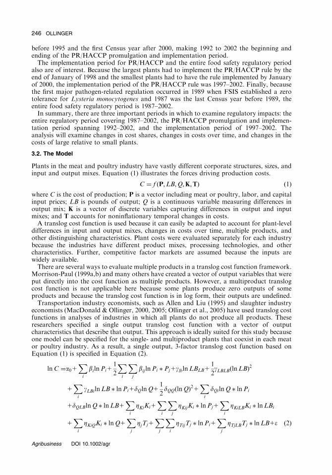
economists (MacDonald & Ollinger, 2000, 2005; Ollinger et al., 2005) have used translog costfunctions in analyses of industries in which all plants do not produce all products. Theseresearchers specified a single output translog cost function with a vector of outputcharacteristics that describe that output. This approach is ideally suited for this study becauseone model can be specified for the single- and multiproduct plants that coexist in each meator poultry industry. As a result, a single output, 3-factor translog cost function based onEquation (1) is specified in Equation (2).

lnC ¼a01X

i

bilnPi11

2

X

i

X

j

bijlnPi � Pj1glblnLBLB11

2gLBLBðlnLBÞ2

1X

i

gLBilnLB � lnPi1dQlnQ11

2dQQðlnQÞ21

X

i

dQilnQ � lnPi

1dQLBlnQ � lnLB1X

i

ZKiKi1X

i

X

j

ZKijKi � lnPj1X

i

ZKiLBKi � lnLBi

1X

i

ZKiQKi � lnQ1X

j

ZjTj1X

j

X

i

ZTijTj � lnPi1X

j

ZTjLBTj � lnLB1e ð2Þ

246 OLLINGER


Efficiency gains are achieved by estimating the cost share equations and cost functionjointly. Share equations equal the derivative of the cost function with respect to input prices(Equation (3)).

@lnC

@lnPi

¼PiXi

C¼ bi1

X

j

bij lnPj1gLBilnLB1dQiQ1X

j

ZjKi1X

j

ZjiTj ð3Þ

Changes in scale economies over time are of particular interest. A measure of scaleeconomies is given by the derivative of the cost function with respect to output—the costelasticity (Equation (4)). The coefficient for the first-order output term, lLB, gives the costelasticity at the sample mean. The coefficient on the second order output term, lLBLB,indicates how scale economies vary with plant size. The other coefficients show how scaleeconomies change with those variables. Changes in economies of scale over time are given bythe interaction of the time dummy variables and output term and would indicate howeconomies of scale changed as the regulatory environment changed.

@lnC

@lnLB¼ gLB1gLBgLBlnLB1

X

i

gLBPilnPi1dQLBlnQ1

X

i

ZKiLBKi1X

J

ZTjLBTj ð4Þ

4. VARIABLE DEFINITIONS AND JUSTIFICATION FOR USE

Variables are defined as follows. Total cost (C) is the sum of labor, meat, and materials, andcapital input expenses. The price of labor (Plabor) is total employee wages and benefits dividedby total employees. The meat and material input price (Pmat) is the cost of the live-weight ofanimals for slaughter plus any packed fresh or frozen meat or poultry plus materials dividedby pounds of meat inputs. The definition of the price of capital (Pcapital) has two componentsand follows Allen and Liu (1995) and MacDonald and Ollinger (2000, 2005), and Ollingeret al. (2005). The first component is the sum of the rental values of machinery and buildingsdivided by their combined book values. Rental values equal rental prices times the bookvalue of assets (either machinery or buildings). Annual capital rental prices are calculated bythe Bureau of Labor Statistics separately for buildings and machinery in the two-digit Foodand Kindred Products Industry Group, using methods described in Chapter 10 of the BLSHandbook of Methods, Bulletin 2490 and on the Multifactor Productivity Web site(stats.bls.gov/mprhome.htm). The measures include changes in asset prices, depreciation,and taxes. The second component is an adjustment cost that equals new investment inbuildings and machinery divided by beginning of year assets.Output (LB) equals pounds of meat and poultry products (all categories in SIC 201). Input

and output mix variables are included in the model because plants use a wide variety ofinputs and produce a number of different outputs and several studies (Antle, 2000;MacDonald & Ollinger, 2000, 2005; Ollinger et al., 2005) have shown that differences ininputs and outputs affect production costs.A continuous output mix variable (Q) is used in the cattle and chicken slaughter models

and resembles one used by MacDonald and Ollinger (2005) and Ollinger et al. (2005). Itequals one minus the share of boxed beef for cattle slaughter and one minus the share ofluncheon meats and other processed poultry minus the share of roasters for chickenslaughter.Discrete input and output mix variables were used by Allen and Lieu (1995) and in other

transportation cost function analyses and by MacDonald and Ollinger (2000, 2005) andOllinger et al. (2005) in slaughter industry studies. The output mix variable K1 is used only forpork processing and sausage-making and equals one if the share of cooked sausages plusfresh sausages plus boiled hams plus cooked hams is greater than zero and zero otherwise inpork processing and equals one if more than 90% of output is a product other than cookedor fresh sausage and zero otherwise in sausage-making. Other output mix variables for



sausage-making and for other industries were tested and dropped because no previous studiessuggested they were important and they did not affect model fit.The variables K2 and K3 capture differences in animal inputs. The variable K2 equals one if

the share of processed meat inputs is greater than zero and zero otherwise in pork processing,one if more than 80% of inputs comes from fresh or frozen meat and zero otherwise insausage-making, one if the share of cattle inputs is less than 0.75 and zero otherwise in cattleslaughter, and one if nonchicken inputs are greater than zero and zero otherwise in chickenslaughter. The input mix variable K3 is used only for chicken slaughter and equals one if theshare of packed meat inputs is greater than zero and zero otherwise. Other input mixvariables were tested and dropped because they did not affect model fit.The remaining variables are defined as follows. The time shift variables T1992, T1997, and

T2002 equal one if the year equals 1992 and zero otherwise, one if the year equals 1997 andzero otherwise, and one if the year equals 2002 and zero otherwise, respectively. There is nodummy variable for 1987 because that is the reference year.

5. DATA

All variables, except capital rental prices were obtained from the Longitudinal ResearchDatabase (LRD) maintained at the Center for Economic Studies of the U.S. Bureau of theCensus. The initial dataset included all meat and poultry plants from Census years, starting in1987 and occurring every 5 years through 2002. Plants from four industries: cattle or chickenslaughter, pork processing, and sausage-making were then extracted from the data to createfour meat and poultry industries. Note that data from the 2007 Census were not used becausethese data were not available when the study was completed.The LRD has data on all plants with more than 20 employees and a sample of thosewith

less than 20 employees. Over 1987–2002, there were 449 cattle slaughter, 521 chickenslaughter and processing, 312 prepared products, and 630 sausage-making plant observationsthat have the complete complement of data.The LRD has data on plant ownership and location and provides detailed information on

employment, wages and benefits, building and machinery asset values, new capitalexpenditures, energy use and costs, the physical quantities and dollar sales of seven-digitSIC code products, and the physical quantities and dollar expenses of detailed materialspurchases. Because the file contains data on individual plants over several Censuses,researchers can make comparisons of different plants during the same year, and can tracechanges in product and input mixes, costs, and industry concentration over time.

6. ESTIMATION AND MODEL SELECTION

Standard practice was followed in estimation. First, symmetry and homogeneity of degreeone were imposed on the model. Second, to simplify interpretation, all variables werenormalized by dividing by their sample means. Third, efficiency gains are achieved byestimating the cost function together with the cost share equations with a nonlinear, iterative,seemingly unrelated regression procedure. Because the costs shares sum to one, thecoefficients of one equation are implied by the other two equations, making it necessary todrop one equation (capital) to avoid a singular covariance matrix. Notice also that the left-and right-hand side variables are defined in current dollars; thus, there is no need to controlfor inflation.A 3-factor cost function including the prices of labor, materials, and capital was used.

A 4-factor cost function that included separate entries for meat and materials was tested butdiscarded because it failed monotonicity tests. In Census data, the identity ‘‘total materialcosts5meat costs1material costs’’ should hold. However, due to widespread datainaccuracies, the identity did not hold in 1997 in the meat and poultry industry, causingthe 4-factor cost function to fail. Models using total materials cost, which includes meat and

248 OLLINGER


material costs, performed well; therefore, a 3-factor cost function was used. Because materialsare a small share of total materials (MacDonald & Ollinger, 2005; Ollinger et al., 2005), totalmaterials mainly reflect meat inputs.Econometricians, such as Maddala et al. (1997), observe that error specification issues arise

in regressions using pooled datasets, making it necessary to check for heteroskedasticity.Using White’s (1980) and Breusch and Pagan (1979) tests, heteroskedasticity was confirmed.As a result, generalized least squares (GLS) and White’s (1980) heteroskedastic consistent-covariance matrix estimator (HCCME) were used to adjust for heteroskedasticity. GLS witha MacKinnon and White (1985) HCCME and the general method of moments were used toconfirm the results. All results are similar. Estimates based on White’s (1980) HCCME arereported in the subsequent tables. The other results are available from the author.Equation (2) is quite general with each variable entering the model in several locations,

complicating variable selection. A number of economists, such as MacDonald and Ollinger(2000, 2005), Antle (2000), and Ollinger et al. (2005), faced a similar problem and used aGallant-Jorgenson (G-J) likelihood ratio test (a chi-square test) to choose the best modelsfrom among sets of restrictive models. That same approach was followed here.In the G-J likelihood test framework, hypotheses are tested by comparing a reference

model against a test model in which test variables are excluded. If the difference in the G-Jstatistic exceeds a statistically significant threshold, the test variables are retained.In each industry, the selection process proceeded by comparing a most-restrictive version of

Equation 2, which includes factor prices and output (P,LB), against the least-restrictivemodel. Then, to evaluate the impact of different variables to model fit, the least-restrictivemodel is compared against models with one or more variables excluded. In cattle slaughter,for example, P,LB was tested against the least-restrictive version of the model, which adds thecontinuous output mix variable (Q), a discrete input mix variable (K2), and time shiftvariables (T) to P,LB to make P,LB,Q, K2,T. Because the difference in the G-J value wassignificant, the restrictive P,LB model was dropped in favor of the less-restrictive model. Insubsequent tests, the time shift variables (T) and continuous output mix (Q) and input mixvariable (K2), were dropped from P,LB,Q, K2,T to create P,LB,Q, K2 and P,LB, T (modelsIII and IV in Table 1) and compared against P,LB,Q, K2,T (model II). In each case, the morerestrictive models were rejected in favor of the less restrictive P,LB,Q, K2,T model. Similarprocedures were performed for other industries, as shown in Table 1.Table 1 gives the G-J test results and all supporting data, including the model number and

description, G-J value, number of parameters estimated, models tested, number ofrestrictions, test variables, and the chi-square statistic for cattle or chicken slaughter, porkprocessing, and sausage-making. Table 1 does not contain all test models because of limitedspace. Other models using variables that proved to be insignificant to model fit were not kept.The best models for each of the four industries are P,LB,Q,K2,T for cattle slaughter,P,LB,Q,K2,K3,T for chicken slaughter, P,LB,K1,K2,T for pork processing, and P,LB,K1,K2,Tfor sausage-making.

7. RESULTS

Model results are given in Tables 2(a) and (b). The R2 statistics are given at the bottom of thetables. Monotonicity is violated in only 2 of the nearly 2,000 observations, and becausemarginal costs are positive for all observations, there are no violations of the regularitycondition.Parameters for the first order terms are given in Table 2(a); Table 2(b) gives the time shift

interaction terms. The parameters on the first order price variables give cost shares in 1987 atthe sample mean size and should be comparable to cost share estimates from other studies.Labor cost shares for all industries varied from 3.8% for cattle to 17.3% for sausage-making.Meat/material shares ranged from 95.0% for cattle slaughter to 75.3% for sausage-making.The capital cost share was very small but remained positive.



The labor share for cattle slaughter is about half the size of the labor share reported byMacDonald and Ollinger (2005) while the meat/material share is correspondingly larger andthe capital share is similar. These differences may be due to a larger percentage of smallplants in this study than in MacDonald and Ollinger (2005). Cost shares for chickenslaughter are nearly identical to those reported in Ollinger et al. (2005).The labor shares should be higher and the meat/materials share lower for the processing

relative to the slaughter industries because more processing requires more labor inputs.Results show that the labor share is more than three times higher and the meat/materialsshare correspondingly lower for the processors relative to cattle slaughter.The coefficient on the output term indicates economies of scale at sample mean prices and

output. Because values less than one indicate economies of scale and the first-order termvaries from 0.816 to 0.915, there are economies of scale at sample mean prices in 1987 (thereference year), a finding that is similar to that reported in MacDonald and Ollinger (2005)Ollinger et al. (2005) for cattle slaughter and chicken slaughter. Finally, the coefficients on Qare negative, as they should be, because Q represents processing steps requiring less effort,such as carcass production. The variables K1, K2, and K3 are input and output mix controlvariables with no expected effects.

7.1. Own and Cross-Price Elasticities

The own price and Allen cross elasticities are reported in Table A1. All of the own priceelasticities are negative except for capital in pork processing, indicating downward sloping

TABLE 1. Gallant-Jorgenson Likelihood Tests Showing Significance of Plant Characteristicsa

Industry Model Description

G-J

value

Parameters

estimated Test Restrictions Test variable w2

Cattle slaughter I P,LBb 979 10 – – –

II (P,LB,Q,K2, T)c 923 32 I vs. II 22 All 56��

III (P,LB,Q, K2)d 950 20 II vs. III 12 Time 27��

IV (P,LB,T)e 961 22 II vs. IV 10 Output mix/

input mixf38��

Chicken slaughter I P,LBb 1443 10 – – –

II (P,LB,Q, K2,K3,T)c 1344 35 I vs. II 25 All 99��

III (P,LB,Q, K2,K3)d 1378 23 II vs. III 12 Time 32��


input mixf71��

Pork processing I P,LBb 788 10 – – –

II (P,LB, K1,K2,T)c 692 30 I vs. II 16 All 96��

III (P,LB, K1,K2)d 721 18 II vs. III 12 Time 29��


input mixf47��

Sausage-making I P,LBb 1760 10 – –

II (P,LB, K1,K2,T)c 1643 30 I vs. II 24 All 117��

III (P,LB, K1,K2)d 1705 18 II vs. III 12 Time 62��


input mixf53��

aThe dependent variable is C (long run costs) in each model.bModel I: base model consisting of prices (P) and pounds of output (LB) and denoted (P, LB).cModel II: Adds time (T), continuous output and input mix variables—Q, K1, K2 and/or K3—to (P, LB) to make (P, LB, Q, K2, T) for

cattle slaughter, (P,LB,Q, K2,K3, T) for chicken slaughter, (P,LB, K1,K2,T) for pork processing, and (P,LB, K1,K2,T) for sausage-

making.dModel III: Removes T from II to make, for example, (P, LB, Q, K2) in cattle slaughter, etc.eModel IV: Removes Q, K1, K2 and/or K3 from II to make (P, LB, T) in cattle slaughter, etc.fOutput and input variables vary by industry.�,��,��significant at the .10, .05, and .01 levels, respectively.

250 OLLINGER


TABLE 2. Cost Function Estimates of Selected Parameters for the 1987–2002 Period

Variable Cattle slaughter Chicken slaughter Pork processing Sausage-making

(a)

Intercept 0.015 0.056�� 0.015 0.110�

(0.027) (0.027) (0.076) (0.061)

T1992 0.039 0.100�� 0.033 0.0003

-1992- (0.04) (0.038) (0.082) (0.043)

T1997 0.033 0.06 0.029 �0.056

-1997- (0.044) (0.041) (0.087) (0.049)

T2002 0.125�� 0.068� 0.108 �0.044

-2002- (0.044) (0.044) (0.096) (0.046)

Plabor 0.038�� 0.167�� 0.124�� 0.173��

(0.009) (0.007) (0.022) (0.017)

Pmat 0.950�� 0.785�� 0.836�� 0.753��

(0.014) (0.012) (0.023) (0.024)

Pcapital 0.012�� 0.048�� 0.04 0.074��

(0.006) (0.016) (0.038) (0.033)

LB 0.915�� 0.816�� 0.856�� 0.901��

(0.018) (0.043) (0.044) (0.037)

LB�LB 0.014� �0.084�� 0.036� 0.002

(0.008) (0.022) (0.021) (0.01)

Q: Continuous �0.503�� 0.096�� – –

output mixb (0.083) (0.023)

K1: Discrete – – 0.052 �0.011

output mixb (0.072) (0.01)

K2: Discrete 0.035 0.043 0.104 �0.0043

input mixc (0.115) (0.035) (0.086) (0.016)

K3: Discrete – �0.06 – –

input mixd (0.065)

R2 0.964 0.904 0.86 0.941

Observations 449 521 312 630

(b) Cost Function Estimates of Time Interaction Parameters for the 1987–2002 Period

T1992� Plabor 0.008 0.005 0.021 0.019�

-1992- (0.015) (0.009) (0.026) (0.012)

T1997� Plabor 0.043�� 0.004 0.022 0.024�

-1997- (0.016) (0.011) (0.028) (0.013)

T2002�Plabor 0.039�� 0.026� 0.021� 0.059��

-2002- (0.015) (0.016) (0.029) (0.013)

T1992� Pmat �0.016 �0.028� �0.038 �0.044��

-1992- (0.019) (0.017) (0.030) (0.017)

T1997� Pmat �0.070�� 0.031� �0.060�� 0.077��

-1997- (0.027) (0.020) (0.028) (0.019)

T2002� Pmat �0.084�� 0.096�� 0.100�� 0.152��

-2002- (0.029) (0.022) (0.038) (0.018)

T1992�Pcapital 0.008 0.023 0.017 0.025

-1992- (0.026) (0.021) (0.046) (0.023)

T1997�Pcapital 0.027 0.027 0.038 0.053��

-1997- (0.038) (0.028) (0.047) (0.026)

T2002�Pcapital 0.045 0.070�� 0.079 0.093��

-2002- (0.036) (0.029) (0.053) (0.025)

T1992� LB 0.032 �0.056 0.00004 �0.030

-1992- (0.024) (0.040) (0.051) (0.023)

T1997� LB 0.003 0.0002 0.038 �0.043�

-1997- (0.021) (0.051) (0.052) (0.025)

T2002� LB �0.013 �0.030 0.002 �0.022

-2002- (0.026) (0.048) (0.057) (0.026)



demand for inputs. Meat/materials for cattle slaughter was quite inelastic but, as expected,more elastic than the meat alone elasticity reported in MacDonald and Ollinger (2005). Alsolike earlier studies (MacDonald & Ollinger, 2000, 2005; Ollinger et al., 2005), the own priceelasticity of meat/materials in chicken slaughter and the processing industries was moreelastic than for cattle slaughter. The labor and capital own price elasticities are much moreelastic than meat/materials in all industries.The Allen elasticity of factor substitution indicates the degree to which a given percent

change in factor ‘‘k’’ can substitute for a percent change in factor ‘‘j.’’ A higher positivenumber indicates greater substitutability. Values are reported in Table A1. The signs of theelasticities are nearly identical across all four industries—positive signs for labor and meat/materials and labor and capital and negative signs for capital and labor.

7.2. Changes in Cost Shares Over Time

MacDonald and Ollinger (2000, 2005) and Ollinger et al. (2005) report that slaughter plantsundertook increasing amounts of processing over the 20 years before 1992, shifting fromproducing carcasses and other low-value products to higher-value items, such as processedmeats and ready-to-cook boneless meat cuts requiring more processing (labor and capitalinputs). This trend continued in the 1990s as many slaughter plants began to promotebranded products.A rise in food safety process control requirements also affected labor and capital inputs. As

reported in Ollinger and Mueller (2003), both consumers and major meat and poultry buyersincreased their demand for stricter food safety process controls during the 1990s. Meanwhile,the PR/HACCP rule of 1996 and other food safety regulations required greater cleaningeffort, production precautions, and quality control monitoring. Both forces—customerdemand and regulation—compelled manufacturers to increase labor and capital inputs,suggesting the labor and capital cost shares should rise and the meat/materials share shoulddrop.The interactions of input prices and the time dummy variables (Table 2(b)) show how cost

shares changed over 1987–2002. The coefficient on the interaction of T2002 with the price oflabor shows that labor shares increased from 2.1 to 5.9% across the four industries over1987–2002. Over 1992–2002, labor shares increased in all industries except pork processing(T2002�PLabor�T1992�PLabor), ranging from 2.1% in chicken slaughter to 4% in sausage-making. Labor share increased 2.2 and 3.5% in chicken slaughter and sausage-making, butdeclined modestly in the other two industries over 1997–2002. Changes were statisticallysignificant over 1987–2002 and 1992–2002, but not over 1997–2002.Changes in the capital costs shares were larger than for labor shares over 1992–2002,

varying from a minimum increase of 3.7% in cattle slaughter to a maximum of 6.8% insausage-making. Changes over 1987–2002 were even larger and those over 1997–2002 weresmaller. All of these changes were statistically significant.The increases in the shares of labor and capital inputs were offset by substantial declines in

the meat/materials share, which fell from between 6.2% in pork processing to 10.8% insausage-making over 1992–2002. Changes over 1987–2002 were larger and over 1997–2002were smaller. These meat share changes were all statistically significant.

TABLE 2. Continued

Variable Cattle slaughter Chicken slaughter Pork processing Sausage-making

R2 0.964 0.904 0.860 0.941

Observations 449 521 312 630

Note. Standard errors are in parentheses. Dependent variable: ln C equals the log of the costs of production. Parameters for the time

interaction terms are reported in Table 2(b). Other second-order terms are not reported, but are available from the author.�, ��, ��significant at the .10, .05, and .01 levels, respectively.

252 OLLINGER


7.3. Changes in Costs Over Time

The impacts of regulation and other events of the 1990s on plant costs over time areevaluated in this section. Plants within industries are compared against each other over time;costs are measured in terms of an index defined relative to costs of a reference plant. Thereference plant is one half the sample mean size in 1987. This size is chosen for convenience;the year is chosen because it preceded all food safety regulations.Table 3 provides an index in which small plant costs (one half the sample mean plant size)

and large plant costs (twice the sample mean plant size) over 1987–2002 are divided by thecosts of the reference plant. The index value for small plants in 1987 (the reference plant-year)is one. Cost index values greater than one indicate higher costs relative to the reference plant-year and values less than one imply lower costs.Four points can be made about costs during three key regulatory periods—1987–2002,

1992–2002, and 1997–2002. First, costs were higher in 2002 than in 1987 in cattle and chickenslaughter and pork processing but not sausage-making. Second, costs for small plants weregenerally greater than one and always greater than the costs of large plants. Third, costs in2002 were higher than in 1992 only in cattle slaughter and pork processing and not in theother two industries. Finally, costs were higher in 2002 than 1997 in all cases and allindustries except large chicken slaughter plants. The cost differences over 1987–2002 and1997––2002 were significant, but cost changes over 1992–2002 were not. Cost differences overperiods not considered critical—1987–1992, 1987–1997, and 1992–1997—were not significant.Only cattle slaughter and pork processing have persistent changes in costs over each of the

three critical time periods—1987–2002, 1992–2002, and 1997–2002. Results for sausage-making indicate no change; chicken slaughter results indicate a rise in costs over the entireperiod but not over 1992–2002.

7.4. Economies of Scale

Changes in economies of scale over time indicate whether the relative costs of large to smallplants are changing. The first-order output term gives a measure of economies of scale atsample mean size and prices in 1987, the interactions of time dummy variables and outputshow how economies of scale change from 1987, and the coefficient on the squared outputterm shows how economies of scale change with plant size.Table 2(a) shows that the coefficients on the first-order output term are below one in all

industries, indicating that economies of scale exist in all industries in 1987 at sample meanprices and output. The negative sign on the squared terms for chicken slaughter suggestsstronger economies of scale with plant size in that industry; the positive signs for the otherindustries imply weaker economies of scale.A positive sign on the interactions of output and the time shift variables moves the

economies of scale parameter closer to one, decreasing economies of scale. A negative sign

TABLE 3. The Production Costs of Small and Large Plants Relative to a Small Plant in 1987 Over 1987–2002

1987 1992 1997 2002

Industry Ratio of plant size to mean size Cost index

Cattle slaughter 0.50 1.000 1.017 1.031 1.143

2.00 0.888 0.944 0.921 0.997

Chicken slaughter 0.50 1.00 1.15 1.06 1.09

2.00 0.77 0.82 0.82 0.81

Pork processing 0.50 1.000 0.967 1.002 1.113

2.00 0.819 0.792 0.866 0.994

Sausage-making 0.50 1.000 0.972 0.974 1.023

2.00 0.871 0.854 0.799 0.821

Note. Small plants equal one half sample mean size; large plants equal twice the sample mean size.



has the reverse effect. Table 2(b) shows that the signs on all of the coefficients for TWO02 �Output in all industries except pork processing are negative, suggesting stronger economies ofscale in 2002 than in 1987. The changes are quite small, ranging from �0.013 in cattleslaughter to �0.030 in chicken slaughter and are not significant.The impact of the PR/HACCP rule of 1996 on economies of scale occurred over the

1992–2002 and 1997–2002 periods. Changes in economies of scale over 1992–2002(T2002�Output�T1992�Output) are positive in all cases except cattle slaughter, suggestingweaker economies of scale in three industries. The negative values for changes in economiesof scale over 1997–2002 (T2002�Output�T1997�Output) for cattle and chicken slaughter andpork processing indicate stronger economies of scale over 1997–2002 but the positive changefor sausage-making suggests weaker economies in that industry. Overall, only cattle slaughtershows persistently stronger economies of scale. The modest and inconsistent changes ineconomies of scale over time for the other industries suggest little or no causal effect of thePR/HACCP rule.

7.5. How Large Plant Long-Run Costs Changed Relative to Small Plants

A relative cost index of large plant costs to small plant cost is shown in Table 4. Of particularinterest are the key regulatory periods: 1987–2002, 1992–2002, and 1997–2002. The relativecost index was constructed by dividing the cost index of the large plants from Table 3 (twicethe sample mean size) by the cost index value of the small plants from Table 3 (one half thesample mean size) for each type of plant in each industry and in each year. For example, theindex value of 0.944, which is given for a cattle slaughter plant in 1992 in Table 3 for a plantthat is twice the sample mean size, is divided by the value of 1.017, which is given for a cattleslaughter plant in 1992 in Table 3 for a plant that is one half the sample mean size. Theresulting ratio of a large plant to small plant cost index value of 0.93 is shown in the first rowof Table 4 in the cell for cattle slaughter plants in 1992. Other values were computed in asimilar manner. Values below one imply that large plants have lower costs than small plants;the reverse is true for values above one. Because all of the computed values are below one,larger plants have lower costs than smaller ones—a finding consistent with numerous articles,including MacDonald and Ollinger (2000, 2005) and Ollinger et al. (2005).Table 4 shows a small drop or no change in the ratios of index values over 1987–2002 in all

industries except pork processing, a decline in the ratios over 1992–2002 in the cattleslaughter and sausage-making and an increase in the other two industries over the sameperiod, and a drop in the ratios in all industries except pork processing over 1997–2002.Only cattle slaughter and sausage-making had declines in their relative cost index ratios

over the three key periods—1987–2002, 1992–2002, and 1997–2002. In chicken slaughter, theratios declined in two periods but rose in one, and, in pork processing, ratios rose in allperiods. Combined with findings that only cattle slaughter had an increase in economies ofscale over the three key periods, these results suggest that the food safety events may havemodestly favored large plants in cattle slaughter throughout the regulatory period andmodestly favored large chicken slaughter plants during the implementation period. This

TABLE 4. The Cost of Production of Large Relative to Small Plants Over 1987–2002

1987 1992 1997 2002

Industry Ratio of cost indexes of large to small plants

Cattle slaughter 0.89 0.93 0.89 0.87

Chicken slaughter 0.78 0.72 0.78 0.74

Pork processing 0.82 0.82 0.86 0.89

Sausage-making 0.87 0.89 0.82 0.80

Note. Cost of production of large relative to small plants equals the cost index of plants of twice the sample mean size divided by the

cost index of plants of one-half the sample mean size. Index values come from Table 3.

254 OLLINGER


finding is consistent with Muth et al. (2007) who found that small meat plants hadmodestly higher plant exit rates during the implementation period of the PR/HACCP rule.The results also make sense when considering the mandated requirements under the PR/HACCP rule. This regulation specified no fixed cost expenditures, established testingrequirements in accordance with slaughter volume, and allowed plants to create their ownHACCP plans, which could allow them to devise scale neutral plans. These characteristicsmade the regulation less onerous to small plants relative to large ones than it may otherwisehave been.There have been studies (Boland et al., 2001; Ollinger & Moore, 2004) showing that

the PR/HACCP rule provides some cost advantages to large plants over small ones.The results presented here are not inconsistent with those results because the earlier analysesdid not allow for any plant cost adjustments. Additionally, short-run cost estimates weremade using food safety cost data and not total production costs, as was considered here. Thisis no small matter because food safety costs are a very small share of the cost of meat orpoultry. More than three fourths of the cost of meat and poultry is comprised of meatand materials.Relative cost differences could also be affected by plant exits. If high-cost plants exited

after the 1997 Census but before the next Census, then those high-cost plants would notappear in the 2002 Census data, and the relative change in costs would be understated.

8. CONCLUSIONS

This study used a translog cost function to examine changes in cost shares, production costs,and the costs of large relative small plants in the cattle slaughter, chicken slaughter, porkprocessing, and sausage-making industries over 1987–2002. This timeframe coincided withimplementation of the PR/HACCP rule of 1996 and two other important food safetyregulations.Results suggest that labor and capital cost shares rose substantially and the meat share of

costs dropped in all industries and that long-run costs rose in cattle slaughter, porkprocessing, and chicken slaughter. There is some evidence that events favored large plantsover small plants in cattle slaughter throughout the period and chicken slaughter during theimplementation period of the PR/HACCP rule. These results are consistent with Muth et al.(2007) who found that the PR/HACCP rule may have encouraged some small meat andpoultry slaughter plants to exit the industry. Results are also consistent with Antle (2000),Ollinger and Mueller (2003), and Hooker, Nayga, and Siebert (2002) who showed thatregulation favored large plants over small ones.The study does not completely isolate costs due to regulatory changes from costs caused by

other events of the 1990s. However, results showing that the relative costs of large to smallplants did not change for pork processing and sausage-making are important becauseregulatory change often favors large over small plants. If the relationship did not change,then regulatory effects must have been small in those two industries. Other results showingthat cost shares changed dramatically and costs rose could be attributed to either regulatorychanges or a shift to greater processing. Regardless, they are important for a betterunderstanding of the meat and poultry industries.

ACKNOWLEDGMENTS

Copyright 2008 is held by the United States Department of Agriculture. All rights reserved.Readers may make verbatim copies of this document for noncommercial purposes by anymeans, provided that this copyright notice appears on all such copies.The judgments and conclusions herein are those of the authors and do not necessarily

reflect those of the U.S. Department of Agriculture. The authors are responsible for allerrors.



APPENDIX A

REFERENCES

Allen, W.B., & Liu, D. (1995). Service quality and motor carrier costs: An empirical analysis. Review of Economicsand Statistics, 77, 499–510.

Antle, J.M. (2000). No such thing as a free lunch: The cost of food safety regulation in the meat industry. AmericanJournal of Agricultural Economics, 82, 310–322.

Ball, V.E., & Chambers, R. (1982). An economic analysis of technology in the meat products industry. AmericanJournal of Agricultural Economics, 62, 699–709.

Boland, M., Peterson-Hoffman, D., & Fox, J.A. (2001). Postimplementation costs of HACCP and SPCPs in GreatPlains meat plants. Journal of Food Safety, 21, 195–204.

Breusch, T., & Pagan, A. (1979). A simple test for heteroskedasticity and random coefficient variation.Econometrica, 47, 1287–1294.

Farber, J.M., & Perterkin, P.I. (1991). Listeria monocytogenes, a food-borne pathogen. Microbiological Reviews,55(4), 476–511.

Hooker, N.H., Nayga, Jr, R.M., & Siebert, J.W. (2002). The impact of HACCP on costs and product exit. Journal ofAgricultural Applied Economics, 34, 165–174.

Knutson, R.D., Cross, H.R., Acuff, G.R., Russell, L.H., Boadu, F.O., Nichols, J.P., et al. (1995). Reforming meatand poultry inspection: Impacts of policy options (IFSE Working Paper 95-1, AFPC Working Paper 95-9).College Station, TX: Texas A&M University, Agricultural and Food Policy Center, Center for Food Safety.

MacDonald, J., & Ollinger, M. (2000). Scale economies and consolidation in hog slaughter. American Journal ofAgricultural Economics, 82(2), 334–346.

MacDonald, J.M., & Ollinger, M. (2005). Technology, labor wars, and producer dynamics: Explaining consolidationin beefpacking. American Journal of Agricultural Economics, 87(4), 1020–1033.

MacKinnon, J., & White, H. (1985). Some heteroskedasticity consistent covariance matrix estimators with improvedfinite sample properties. Journal of Econometrics, 19, 305–325.

Maddala, G.S., Trost, R.R., Li, H., & Joutz, F. (1997). Estimation of short-run and long-run elasticities of energydemand from panel data using shrinkage estimators. Journal of Business and Economic Statistics, 15, 90–100.

Melton, B.E., & Huffman, W.E. (1995). Beef and pork packing costs and input demands: Effects of unionization andtechnology. American Journal of Agricultural Economics, 77, 471–485.

Morrison-Paul, C.J. (1998). Cost economies and market power in U.S. meat packing. Report to the U.S. Departmentof Agriculture, Grain Inspection, Packers, and Stockyards Administration. Washington, DC: U.S. Department ofAgriculture.

TABLE A1. 1987 Input Shares, Own Factor Price Elasticities, and Allen Cross Elasticities

Price

Industry Price Labor Meat/materials Capital

Cattle slaughter Input share 0.079 0.885 0.036

eij (Own price elasticity) �1.025 �0.061 �0.655

sij (Allen cross elasticity) Labor �0.662 1.222 �12.158

Meat/materials – 0.989 1.175

Capital – – 28.778

Chicken slaughter Input share 0.181 0.742 0.077


sij (Allen cross elasticity) Labor �2.784 0.748 �1.994

Meat/materials �0.279 0.894

Capital �7.260

Pork processing Input share 0.179 0.723 0.098

eij (Own price elasticity) �0.416 �0.095 0.265

sij (Allen cross elasticity) Labor 4.707 0.682 �3.286

Meat/materials 1.083 0.252

Capital 31.625

Sausage-making Input share 0.217 0.677 0.106


sij (Allen cross elasticity) Labor 5.452 0.731 �0.718

Meat/materials 1.079 0.821

Capital 6.661

256 OLLINGER


Morrison-Paul, C.J. (1999a). Cost structure and the measurement of economic performance: Productivity,utilization, cost economics, and related performance indicators. Boston: Kluwer.

Morrison-Paul, C.J. (1999b). Scale effects and mark-ups in the U.S. food and fibre industries: Capital investment andimport penetration impacts. The Journal of Agricultural Economics, 55, 64–82.

Muth, M.K., Wohlgenant, M.K., & Karns, S.A. (2007). Did the Pathogen Reduction and Hazard Analysis andCritical Control Points Regulation cause slaughter plants to exit? Review of Agricultural Economics, 29, 596–611.

Muth, M.K., Wohlgenant, M.K., Karns, S.A., & Anderson, D.W. (2003). Explaining plant exit in the U.S. meat andpoultry industries. Journal of Agricultural and Food Industrial Organization, 1, 1–21.

Muth, M.K., Karns, S.A., Wohlgenant, M.K., & Anderson, D.W. (2002). Exit of meat slaughter plants duringimplementation of the PR/HACCP regulations. Journal of Agricultural and Resource Economics, 27, 187–203.

Nganje, W., & Mazzocco, M.A. (2000). Economic efficiency analysis of HACCP in the U.S. red meat industry. InL.J. Unnevehr (Ed.), Economics of HACCP: Costs and benefits (pp. 241–266). St. Paul, MN: Eagan Press.

Ollinger, M., Moore, D., & Chandran, R. (2004). Meat and poultry plants’ food safety investments: Survey findings(ERS Technical Bulletin 1911). Washington, DC: U.S. Departmednt of Agriculture, Economic Research Service.

Ollinger, M., & Mueller, V. (2003). Managing for safer food: The economics of sanitation and process controls inmeat and poultry plants (Agricultural Economic Report 817). Washington, DC: U.S. Department of Agriculture,Economic Research Service.

Ollinger, M., MacDonald, J., & Madison, M. (2005). Technological change and economies of scale in U.S. poultryprocessing. American Journal of Agricultural Economics, 87(1), 116–129.

Perl, P. (2000, January 16). Outbreak: Poisoned package. Washington Post Magazine, pp. 7–27.U.S. Department of Labor, Bureau of Labor Statistics. (1992). BLS handbook of methods. Bulletin 2414

(September). Washington, DC.U.S. Bureau of the Census. (1987–2002). Longitudinal research database. Washington, DC: Author.White, H. (1980). A heteroskedasticity-consistent covariance matrix estimator and a direct test for heteroskedasticity.

Econometrica, 48, 817–838.

Michael Ollinger is an economist at the Economic Research Service of the United States Department of

Agriculture, Washington, DC. He graduated from Washington University in St. Louis with a Ph.D. in

1991. His current areas of research are food safety, structural change, and the costs of school meals.



structural change in the meat and poultry industry and food safety regulations

Documents