structural health monitoring via stiffness update …home.iitk.ac.in/~vinaykg/iset509.pdf · 48...

ISET Journal of Earthquake Technology, Paper No. 509, Vol. 47, No. 1, March 2010, pp. 47–60

STRUCTURAL HEALTH MONITORING VIA STIFFNESS UPDATE

Prashant V. Pokharkar and Manish Shrikhande Department of Earthquake Engineering Indian Institute of Technology Roorkee

Roorkee–247667

ABSTRACT

The performance of an updated time-domain least-squares identification method for identifying a reduced-order linear system model in the case of limited response measurements and its use in structural health monitoring is evaluated. It is shown that the incorporation of a mass-invariability constraint enhances the robustness of the parametric identification procedure. The full structural stiffness and mass matrices are identified from the identified reduced-order model by using the condensed model identification and recovery method. The damage state is considered to be represented by an incremental stiffness degradation model. The degradation in stiffness is estimated through the minimization of an error function defined in terms of Rayleigh quotients. The performance of the proposed scheme is examined with reference to the simulated damage due to earthquake excitation in a 10-story building with rigid floor diaphragm.

KEYWORDS: Detection, Dynamic Condensation, Least-Squares Identification, Structural Health Monitoring, System Identification

INTRODUCTION

Structural system identification has gained in importance over the last couple of years as a diagnostic tool for the structural health assessment—primarily due to the requirements of enhanced functionality and reduced downtime of buildings and services. The conventional approaches to structural health assessment require physical access to the regions of interest in the structural system and are also very tedious and time consuming. The damage/degradation in structures causes reduction of natural frequencies, increased energy dissipation, and changes in the mode shapes. Therefore, monitoring of vibration characteristics of structural system should permit the detection of both the location and severity of damage. The vibration-based system identification and health assessment is promising because substantial information can be gathered by only a few sensors distributed across the structural system. The system identification approaches can be classified as either parametric or non-parametric methods. In parametric methods, the structural models to be identified are characterized in terms of a finite set of parameters, such as the coefficients of the governing differential equations of motion, or the coefficients of the rational polynomial approximation for transfer function, etc. The non-parametric methods, on the other hand, characterize the dynamic systems in terms of impulse response functions, or frequency response functions derived from the direct measurements of excitation and response at various locations in the structural system. As the stiffness characteristics are most prominently influenced by the damage, if any, in the structural systems, several approaches have been developed to identify stiffness, or related characteristics of a structural system from the analysis of its vibration signatures. Udwadia (2005) presented a method for the identification of the stiffness matrices of a structural system from the information about some of its observed frequencies and corresponding mode shapes of vibration. Pandey and Biswas (1994) suggested the use of mode shape curvature in detecting damage. For large and/or complex structures, however, the changes in mode shapes and their curvatures may be so small that their use for the detection of damage might not be practical. Stubbs et al. (1995) developed a methodology based on the comparison of modal strain energy before and after damage to identify damage in structure. However, except for very simple structures, moderate damage does not significantly affect the lower modes of vibration, which can be identified with greater reliability. Baruch and Bar Itzhack (1978) proposed a matrix update method, wherein a norm of the global parameter matrix perturbations is minimized with the application of symmetry constraint on property matrix. Many other approaches developed in this area are based on the

48 Structural Health Monitoring via Stiffness Update

minimization of the rank of perturbed matrix with connectivity and sparsity constraint on the original matrix. In large scale complex structural systems the natural frequencies and mode shapes towards the higher end of the spectrum can rarely be identified with sufficient accuracy, which in turn affect the reliability of damage detection on the basis of mode shape information. Agbabian et al. (1990) and Smyth et al. (2000) proposed a least-squares method for the parametric identification of a linear system for estimating the coefficients of the governing differential equation. For a limited number of sensors to record the vibration response, the time-domain least-squares identification procedure yields the minimum norm estimates for the coefficients of the reduced order system, which may be significantly different from the ‘true’ coefficients (Choudhury, 2007). This problem of non-uniqueness of the results of time-domain least-squares identification procedure is addressed in this study. Reduced-order equivalent linear models are identified for different time windows. The full system matrices are recovered from the estimated reduced order models and an attempt is made to detect the presence of damage by tracking the changes in the stiffness coefficients of the recovered full stiffness matrix of the structure. The performance of this scheme is examined with the help of a simple analytical model for a steel structural frame with rigid floor diaphragms and subjected to earthquake excitation.

TIME-DOMAIN LEAST-SQUARES IDENTIFICATION

Let us consider the governing equations of motion for a multi-degree-of-freedom (MDOF) system subjected to the external forces { }f :

[ ]{ } [ ]{ } [ ]{ } { }+ + =M y C y K y f (1)

where, [ ]M , [ ]C and [ ]K are the mass, damping and stiffness matrices of the system and { }y represents the vector of deformations at each degree of freedom (DOF). In practice, the system response is recorded only at a few select DOFs corresponding to the sensor locations, and we consider these DOFs as primary (or master) DOFs. The least-squares parametric identification would allow us to estimate the coefficients of the reduced-order model consisting only of the primary DOFs. By partitioning the vector

of deformations as { } { } { }{ },=TTT

s py y y , where { }py and { }sy denote the primary and secondary

DOFs, respectively, the system considered for identification is

{ } { } { } { } + + ≈ p p p pM y C y K y f (2)

where, M , C and K denote the inertia, damping and stiffness characteristics of the structural

system after condensing out the secondary DOFs. The vector { }pf represents the equivalent forces on the

primary DOFs and depends on the transformation of the full analytical model of Equation (1) to the reduced-order model of Equation (2). Assuming that a total of pn number of response measurements are

available at different sensor locations, a vector of responses, say { } 1 3( )×∈ pnir , at the i th time instant

can be constructed as

{ } { }11 1( ) ( ) ( ) ( ) ( ) ( )= , ,p p pi i n i i n i i n ir t …y t t …y t y t …y ty y (3)

Considering the response at all time instants ( 1t through nt ), a response matrix [ ] 3( )×∈ pn nR can be defined as

[ ]

{ }{ }

{ }

1

2

= n

rr

R

r

(4)

The coefficients of Equation (2) corresponding to each primary DOF may be arranged as

ISET Journal of Earthquake Technology, March 2010 49

{ } { }1 1 1, , , , , , , , ;= … … …p p pj j jn j jn j jnm m c c k kα 1 2= , , , pj … n (5)

where 1jm , 1jc and 1jk , respectively, denote the coefficients of the condensed system matrices M ,

C and K , and { } 1 3( )×∈ pnjα is the arrangement of these coefficients of the j th row in a row

vector. Equation (2) can then be rearranged in the form:

{ } { }ˆˆ ˆ = R bα (6)

where 23ˆ ( )× ∈

p pnn nR is a block diagonal matrix with the response matrix [ ]R on its diagonal, { }α̂

23 1( ;×∈ pn { } { }{ },= ,p

T

j n…α α ), and { } 1ˆ ( )×∈ pnnb is the vector of corresponding excitation

measurements given by

{ }{ }

{ }

1

2ˆ

= pn

bb

b

b

(7)

with { } ( ) ( ) ( ){ }1 2, , ,= …T

j j j j nb f t f t f t , 1 2 .= , , , pj … n Here, ( )j if t , 1 2= , , , pj … n denotes the

equivalent forces on the primary degrees of freedom of the condensed system at time it and are described in the following section. The least-squares solution of Equation (6) may be then obtained as

{ } { }† ˆˆˆ = R bα (8)

where †ˆ R is the Moore-Penrose pseudo-inverse (Golub and Van Loan, 1996) of ˆ . R The least-

squares solution computed in Equation (8) corresponds to the solution of associated normal equations

( { } { }ˆˆ ˆ ˆˆ = T T

R R R bα ). The solution vector { }α̂ provides the minimum-norm least-squares

estimates of the desired system parameters. It is often required to improve the numerical conditioning of the system of equations and also to impose the constraint of symmetry of coefficient matrices to eliminate physically inconsistent results of system identification.

ANALYTICAL REDUCTION OF SYSTEM MATRICES

Since the above-mentioned time-domain least-squares parametric identification procedure can only identify a reduced-order model corresponding to the primary DOFs (Smyth et al., 2000), it is desirable to have a set of benchmark values for assessing the quality of parameter estimates before using the results of this identification procedure to draw further inferences. A comparable reduced-order system model can be obtained by the elimination of secondary DOFs from the system of equations by using the dynamic condensation method (Paz, 1984, 2004). Let us write the equations of motion for free vibration in partitioned matrix form as

[ ] [ ] { }

{ }{ }{ }

2 2

2 2

00

− − = − −

ss i ss sp i sp s

pps i ps pp i pp

K M K M yyK M K M

ω ω

ω ω (9)

from which the secondary variables can be eliminated as

{ } [ ] [ ]( ) ( ){ } [ ]{ }12 2− = − − − = s ss i ss sp i sp p i py K M K M y T yω ω (10)


where 2iω is an approximation for the i th eigenvalue of the structural system, and [ ] =iT

[ ] [ ]( ) ( )12 2− − − − ss i ss sp i spK M K Mω ω represents the transformation matrix relating the primary

(master) DOFs to the secondary (slave) DOFs for the current approximation of the i th eigenvalue obtained from the reduced-order system containing only primary DOFs. The full DOFs-vector

{ } { }{ },TTT

s py y may be then expressed in terms of the primary DOFs as

{ }{ }

[ ][ ] { } { }

= =

s ip i p

p

y Ty T y

Iy (11)

where [ ]I denotes an identity matrix and iT is the matrix relating the full-DOFs vector to the primary

DOFs. The reduced mass and stiffness matrices are then obtained as

[ ] = T

i i iM T M T and 2i i iK D Mω = + (12)

with

( ) ( )[ ]2 2 = − + − pp i pp ps i ps iD K M K M Tω ω (13)

These reduced-order system matrices are used to calculate an improved estimate of the i th eigenvalue, which is then substituted in Equation (13) and the iterative process is repeated until the eigenvalue is close enough to that for the full model. This process may be repeated for estimating the next eigenvalue. Since the reduced mass and stiffness matrices are influenced by the choice of natural frequency, an iterative scheme is necessary to converge to a set of reduced matrices which have the same natural frequencies in the lower half of the spectrum as those calculated for the full-order system. The final reduced-order matrices can be used for the modeling of the forced vibration problem, for which the response is only monitored at the primary DOFs. The modified force vector for the reduced-order model in the case of excitation by base motion may be expressed as

{ }[ ]

{ }1 ( ) = −

ss spT

p i g

ps pp

M Mf T u t

M M (14)

where iT is the transformation relating the DOFs of the chosen reduced-order analytical model to the

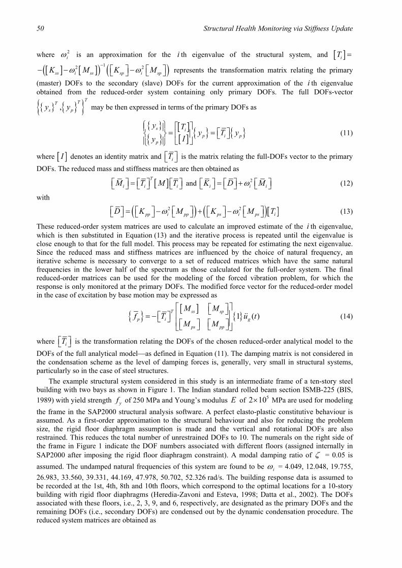
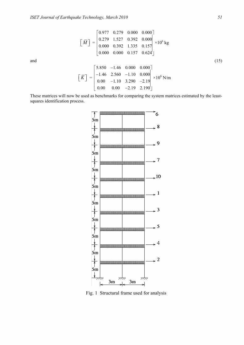
DOFs of the full analytical model—as defined in Equation (11). The damping matrix is not considered in the condensation scheme as the level of damping forces is, generally, very small in structural systems, particularly so in the case of steel structures. The example structural system considered in this study is an intermediate frame of a ten-story steel building with two bays as shown in Figure 1. The Indian standard rolled beam section ISMB-225 (BIS, 1989) with yield strength yf of 250 MPa and Young’s modulus E of 52 10× MPa are used for modeling the frame in the SAP2000 structural analysis software. A perfect elasto-plastic constitutive behaviour is assumed. As a first-order approximation to the structural behaviour and also for reducing the problem size, the rigid floor diaphragm assumption is made and the vertical and rotational DOFs are also restrained. This reduces the total number of unrestrained DOFs to 10. The numerals on the right side of the frame in Figure 1 indicate the DOF numbers associated with different floors (assigned internally in SAP2000 after imposing the rigid floor diaphragm constraint). A modal damping ratio of ζ = 0.05 is assumed. The undamped natural frequencies of this system are found to be iω = 4.049, 12.048, 19.755, 26.983, 33.560, 39.331, 44.169, 47.978, 50.702, 52.326 rad/s. The building response data is assumed to be recorded at the 1st, 4th, 8th and 10th floors, which correspond to the optimal locations for a 10-story building with rigid floor diaphragms (Heredia-Zavoni and Esteva, 1998; Datta et al., 2002). The DOFs associated with these floors, i.e., 2, 3, 9, and 6, respectively, are designated as the primary DOFs and the remaining DOFs (i.e., secondary DOFs) are condensed out by the dynamic condensation procedure. The reduced system matrices are obtained as


M =

0 977 0 279 0 000 0 0000 279 1 527 0 392 0 0000 000 0 392 1 335 0 1570 000 0 000 0 157 0 624

. . . . . . . . . . . . . . . .

×106 kg

and (15)

K =

5 850 1 46 0 000 0 0001 46 2 560 1 10 0 000

0 00 1 10 3 290 2 190 00 0 00 2 19 2 190

. − . . . − . . − . . . − . . − . . . − . .

×108 N/m

These matrices will now be used as benchmarks for comparing the system matrices estimated by the least-squares identification process.

Fig. 1 Structural frame used for analysis


DATASET FOR SYSTEM IDENTIFICATION

In the time-domain least-squares system identification approach, it is necessary to have the excitation and the response data of the system. The building response data is generated through a non-linear dynamic analysis of an analytical model in the SAP2000 environment. The dataset consists of relative displacement, relative velocity and relative acceleration responses at each of the designated floors assumed to have vibration sensors, namely, the 1st, 4th, 8th and 10th (roof) floors. A scaled time history (with the scale factor of 2) of the Northridge, California earthquake ground motion recorded at Pacoima Dam Upper Left Abutment (with the closest distance of 8 km to the fault rupture) on January 17, 1994 for the component 104 (as in the PEER database1) and sampling interval of 0.02 s is considered as the base excitation. This ground motion has the peak ground acceleration (PGA) of 1.58g. Figure 2 shows the (unscaled) time history of this ground motion.

Fig. 2 Northridge earthquake ground acceleration time history

The recorded time history is scaled (by a factor of 2) to enforce the development of plastic hinges in the structural frame during the shaking. A zero-mean Gaussian random noise is added to simulate the effect of measurement noise such that nσ = 0.05 ,sσ where nσ denotes the standard deviation of noise and sσ represents the standard deviation of the actual time-domain signal. A representative plot of the computed relative acceleration, velocity and displacement time histories at the 10th floor is shown in Figure 3. All time histories are sampled at 0.02 s interval. In the case of seismic excitations, response data is generally acquired by using accelerometers, which record absolute accelerations at the base of the transducers. The relative acceleration response is then obtained by subtracting the base acceleration from the recorded floor accelerations. The velocity and displacement time histories are obtained by integrating the acceleration time history filtered to correct for baseline errors. These time histories are then used for the least-squares system identification. However, considering the full-duration data at once smears away the time-varying information and one only gets gross time-averaged information to draw inferences. Since the damage of building frame during an earthquake is a gradual process, it is expected that this effect should be noticeable in the parameter estimates obtained from the data segments from small time windows. The length of the data window is an important consideration for any such moving window analysis and is decided by examining the temporal evolution of the frequency content in the structural response time history. The temporal evolution is depicted by the spectrogram, i.e., the plot of the squared amplitude of the short time Fourier transform (STFT) of the response time history. The STFT of a signal may be defined as

( ) ( ) ( ) d∞ −

−∞, = −∫ iwuSf t f u g u t e uω (16)

1 Website of PEER Strong Motion Database, http://peer.berkeley.edu/smcat/ (last accessed on January 2, 2010)


where ( )g u t− denotes a real, symmetric window in time domain and serves to localize the Fourier integral in the neighbourhood of u = .t The spectrogram is defined as the energy density of the STFT as

2( ) ( ), = ,S t Sf tω ω (17)

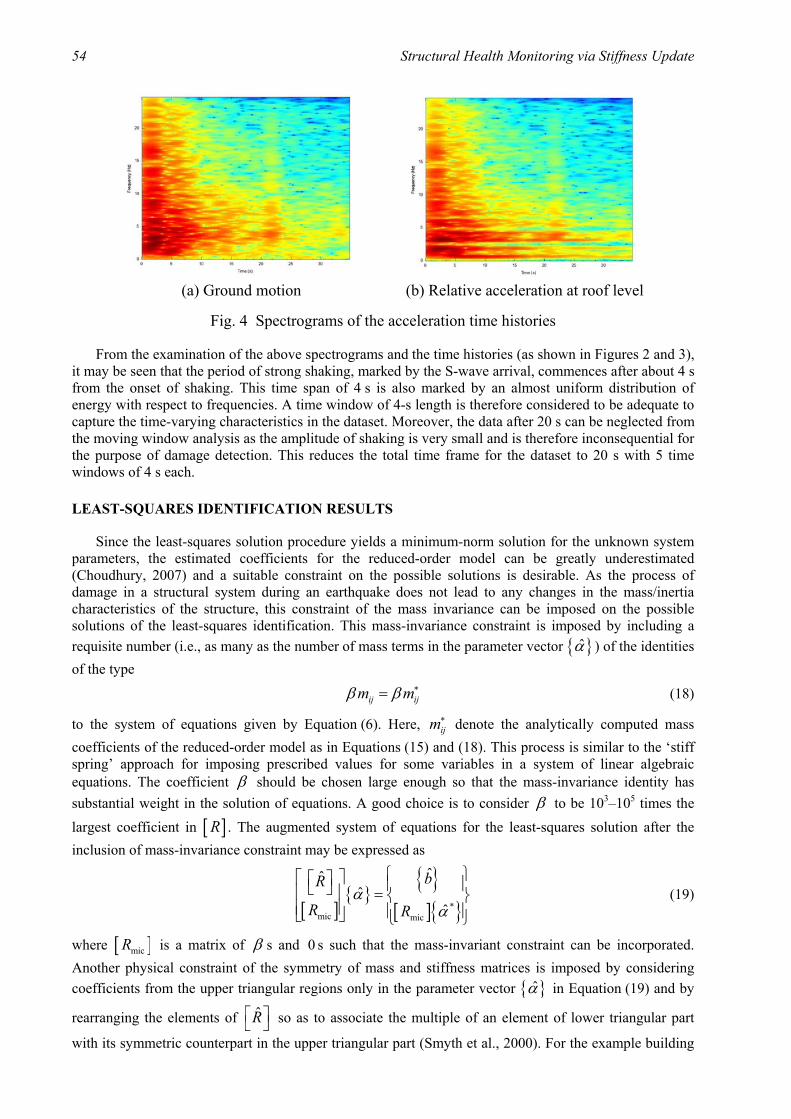
The length of window function is an important factor in STFT-based time-frequency analyses—too short a window enhances the resolution in time at the cost of poor resolution in frequency domain, whereas too long a window provides a sharp spectral resolution with low resolution in time domain. In this study a 256-sample Hann window with 0.9 overlap factor is used for calculating spectrograms. The variation of the energy of various harmonics in a signal with respect to time is color coded with large amplitudes shown in red to very small amplitudes shown in violet colour. Figure 4 shows the spectrograms of the ground motion and the relative acceleration response at the roof level of the example building.

Fig. 3 Computed relative acceleration, velocity and displacement time histories at the 10th floor


(a) Ground motion (b) Relative acceleration at roof level

Fig. 4 Spectrograms of the acceleration time histories

From the examination of the above spectrograms and the time histories (as shown in Figures 2 and 3), it may be seen that the period of strong shaking, marked by the S-wave arrival, commences after about 4 s from the onset of shaking. This time span of 4 s is also marked by an almost uniform distribution of energy with respect to frequencies. A time window of 4-s length is therefore considered to be adequate to capture the time-varying characteristics in the dataset. Moreover, the data after 20 s can be neglected from the moving window analysis as the amplitude of shaking is very small and is therefore inconsequential for the purpose of damage detection. This reduces the total time frame for the dataset to 20 s with 5 time windows of 4 s each.

LEAST-SQUARES IDENTIFICATION RESULTS

Since the least-squares solution procedure yields a minimum-norm solution for the unknown system parameters, the estimated coefficients for the reduced-order model can be greatly underestimated (Choudhury, 2007) and a suitable constraint on the possible solutions is desirable. As the process of damage in a structural system during an earthquake does not lead to any changes in the mass/inertia characteristics of the structure, this constraint of the mass invariance can be imposed on the possible solutions of the least-squares identification. This mass-invariance constraint is imposed by including a requisite number (i.e., as many as the number of mass terms in the parameter vector { }α̂ ) of the identities of the type

ij ijm mβ β ∗= (18)

to the system of equations given by Equation (6). Here, ijm∗ denote the analytically computed mass coefficients of the reduced-order model as in Equations (15) and (18). This process is similar to the ‘stiff spring’ approach for imposing prescribed values for some variables in a system of linear algebraic equations. The coefficient β should be chosen large enough so that the mass-invariance identity has substantial weight in the solution of equations. A good choice is to consider β to be 103–105 times the largest coefficient in [ ]R . The augmented system of equations for the least-squares solution after the inclusion of mass-invariance constraint may be expressed as

[ ]

{ }{ }

[ ]{ }*mic mic

ˆˆˆ

ˆ

=

bR

R Rα

α (19)

where [ ]micR is a matrix of β s and 0 s such that the mass-invariant constraint can be incorporated. Another physical constraint of the symmetry of mass and stiffness matrices is imposed by considering coefficients from the upper triangular regions only in the parameter vector { }α̂ in Equation (19) and by

rearranging the elements of ˆ R so as to associate the multiple of an element of lower triangular part

with its symmetric counterpart in the upper triangular part (Smyth et al., 2000). For the example building


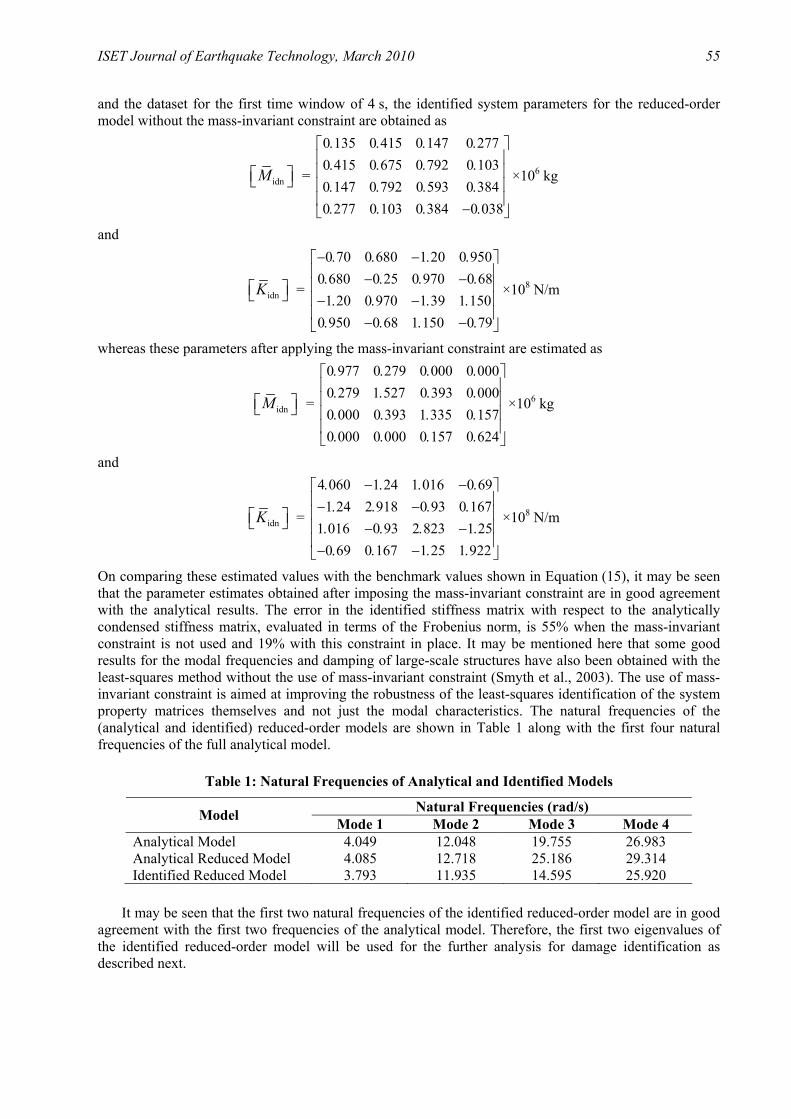
and the dataset for the first time window of 4 s, the identified system parameters for the reduced-order model without the mass-invariant constraint are obtained as

idn M =

0 135 0 415 0 147 0 2770 415 0 675 0 792 0 1030 147 0 792 0 593 0 3840 277 0 103 0 384 0 038

. . . . . . . . . . . . . . . − .

×106 kg

and

idn K =

0 70 0 680 1 20 0 9500 680 0 25 0 970 0 68

1 20 0 970 1 39 1 1500 950 0 68 1 150 0 79

− . . − . . . − . . − . − . . − . . . − . . − .

×108 N/m

whereas these parameters after applying the mass-invariant constraint are estimated as

idn M =

0 977 0 279 0 000 0 0000 279 1 527 0 393 0 0000 000 0 393 1 335 0 1570 000 0 000 0 157 0 624

. . . . . . . . . . . . . . . .

×106 kg

and

idn K =

4 060 1 24 1 016 0 691 24 2 918 0 93 0 167

1 016 0 93 2 823 1 250 69 0 167 1 25 1 922

. − . . − . − . . − . . . − . . − . − . . − . .

×108 N/m

On comparing these estimated values with the benchmark values shown in Equation (15), it may be seen that the parameter estimates obtained after imposing the mass-invariant constraint are in good agreement with the analytical results. The error in the identified stiffness matrix with respect to the analytically condensed stiffness matrix, evaluated in terms of the Frobenius norm, is 55% when the mass-invariant constraint is not used and 19% with this constraint in place. It may be mentioned here that some good results for the modal frequencies and damping of large-scale structures have also been obtained with the least-squares method without the use of mass-invariant constraint (Smyth et al., 2003). The use of mass-invariant constraint is aimed at improving the robustness of the least-squares identification of the system property matrices themselves and not just the modal characteristics. The natural frequencies of the (analytical and identified) reduced-order models are shown in Table 1 along with the first four natural frequencies of the full analytical model.

Table 1: Natural Frequencies of Analytical and Identified Models

Natural Frequencies (rad/s) Model Mode 1 Mode 2 Mode 3 Mode 4 Analytical Model 4.049 12.048 19.755 26.983 Analytical Reduced Model 4.085 12.718 25.186 29.314 Identified Reduced Model 3.793 11.935 14.595 25.920

It may be seen that the first two natural frequencies of the identified reduced-order model are in good agreement with the first two frequencies of the analytical model. Therefore, the first two eigenvalues of the identified reduced-order model will be used for the further analysis for damage identification as described next.


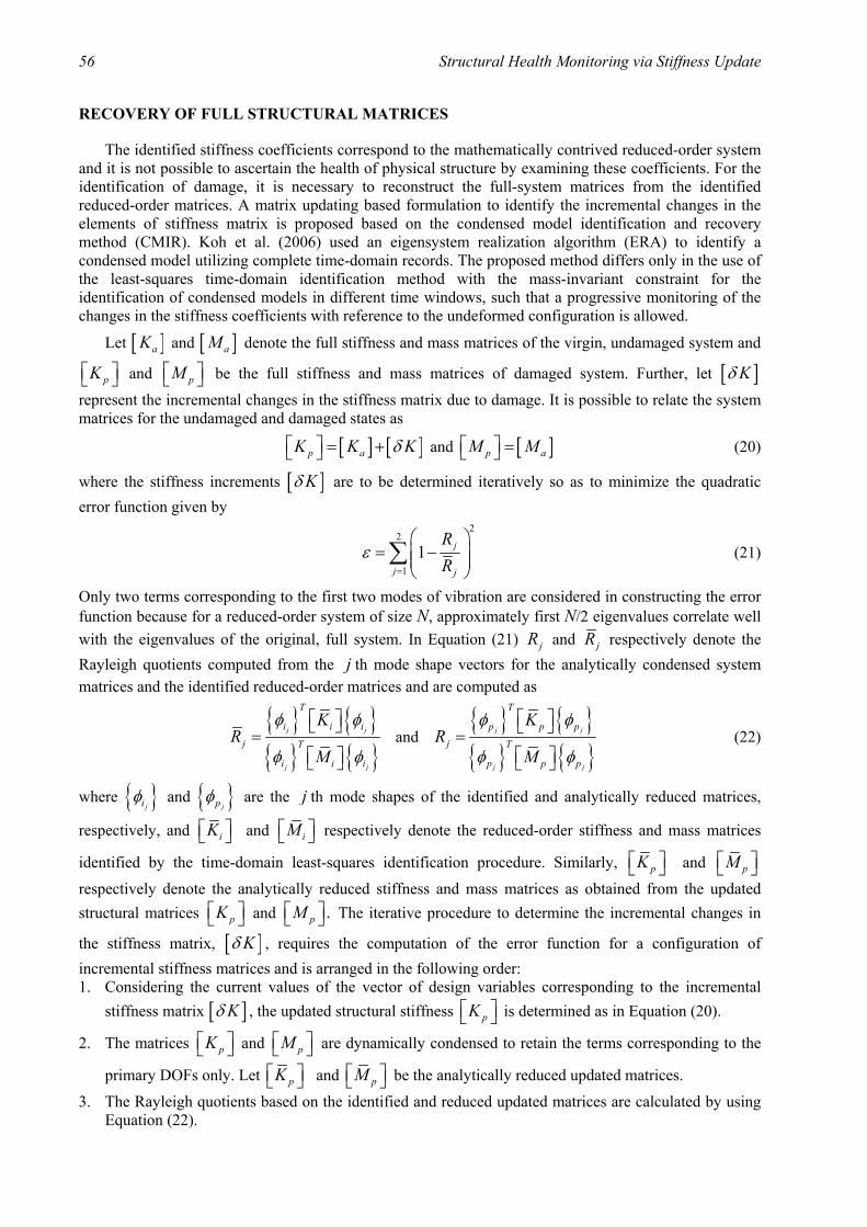
RECOVERY OF FULL STRUCTURAL MATRICES

The identified stiffness coefficients correspond to the mathematically contrived reduced-order system and it is not possible to ascertain the health of physical structure by examining these coefficients. For the identification of damage, it is necessary to reconstruct the full-system matrices from the identified reduced-order matrices. A matrix updating based formulation to identify the incremental changes in the elements of stiffness matrix is proposed based on the condensed model identification and recovery method (CMIR). Koh et al. (2006) used an eigensystem realization algorithm (ERA) to identify a condensed model utilizing complete time-domain records. The proposed method differs only in the use of the least-squares time-domain identification method with the mass-invariant constraint for the identification of condensed models in different time windows, such that a progressive monitoring of the changes in the stiffness coefficients with reference to the undeformed configuration is allowed.

Let [ ]aK and [ ]aM denote the full stiffness and mass matrices of the virgin, undamaged system and

pK and pM be the full stiffness and mass matrices of damaged system. Further, let [ ]Kδ

represent the incremental changes in the stiffness matrix due to damage. It is possible to relate the system matrices for the undamaged and damaged states as

[ ] [ ] = + p aK K Kδ and [ ] = p aM M (20)

where the stiffness increments [ ]Kδ are to be determined iteratively so as to minimize the quadratic error function given by

2

2

11

=

= −

∑ j

j j

RR

ε (21)

Only two terms corresponding to the first two modes of vibration are considered in constructing the error function because for a reduced-order system of size N, approximately first N/2 eigenvalues correlate well with the eigenvalues of the original, full system. In Equation (21) jR and jR respectively denote the Rayleigh quotients computed from the j th mode shape vectors for the analytically condensed system matrices and the identified reduced-order matrices and are computed as

{ } { }{ } { }

=

j j

j j

T

i i i

j T

i i i

KR

M

φ φ

φ φ and

{ } { }{ } { }

=

j j

j j

T

p p p

j T

p p p

KR

M

φ φ

φ φ (22)

where { }jiφ and { }jpφ are the j th mode shapes of the identified and analytically reduced matrices,

respectively, and iK and iM respectively denote the reduced-order stiffness and mass matrices

identified by the time-domain least-squares identification procedure. Similarly, pK and pM

respectively denote the analytically reduced stiffness and mass matrices as obtained from the updated structural matrices pK and . pM The iterative procedure to determine the incremental changes in

the stiffness matrix, [ ]Kδ , requires the computation of the error function for a configuration of incremental stiffness matrices and is arranged in the following order: 1. Considering the current values of the vector of design variables corresponding to the incremental

stiffness matrix [ ]Kδ , the updated structural stiffness pK is determined as in Equation (20).

2. The matrices pK and pM are dynamically condensed to retain the terms corresponding to the

primary DOFs only. Let pK and pM be the analytically reduced updated matrices.

3. The Rayleigh quotients based on the identified and reduced updated matrices are calculated by using Equation (22).


4. The error function for the current estimate of the incremental matrix [ ]Kδ is calculated by using Equation (21).

Due to the symmetry of the stiffness matrix, only the upper triangular elements of [ ]Kδ are considered as the design variables—a total of 19 elements for a 10-story building with rigid floor diaphragms—for the minimization problem. The design variables are numbered row-wise for the upper triangular part of [ ].Kδ The sequential quadratic programming is used to minimize the error function defined in Equation (21) with respect to the design variables, i.e., stiffness increments. The upper and lower bounds on the stiffness coefficients are chosen to be 0 and 30% of the original stiffness coefficients, with negative sign added to indicate the nature of stiffness degradation with damage. The starting vector to begin the optimization process is picked by randomly choosing the design variables from the given range. To guard against the possibility of converging on a local minimum, the minimization process is repeated 40 times with randomly selected initial design vectors. The set of design variables corresponding to the minimum ε (in 40 trials) is assumed to give the desired incremental matrix. This procedure is carried out for all the five time windows. The values of variables obtained for these windows after optimization are shown in Figure 5 and Table 2.

(a) First window (0-4 s)

(b) Second window (4-8 s)

(c) Third window (8-12 s)

(d) Fourth window (12-16 s)

(e) Fifth window (16-20 s)

Fig. 5 Final values of design variables for different time windows


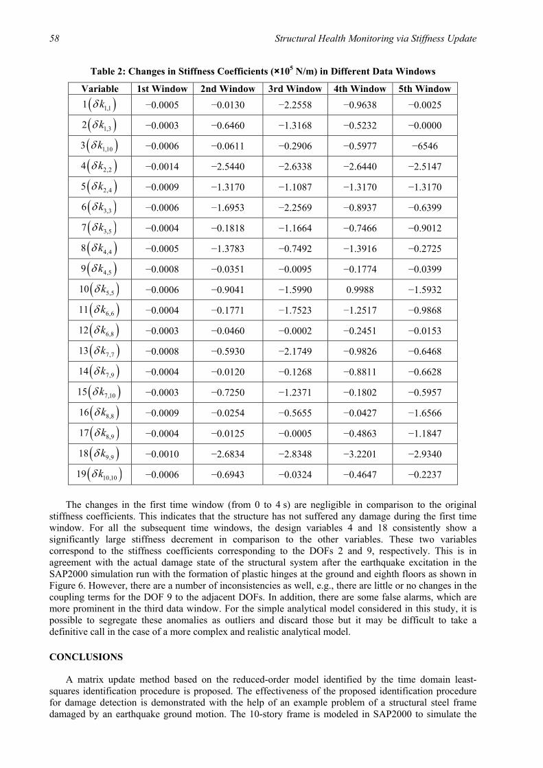
Table 2: Changes in Stiffness Coefficients (×105 N/m) in Different Data Windows

Variable 1st Window 2nd Window 3rd Window 4th Window 5th Window 1 ( )1,1kδ −0.0005 −0.0130 −2.2558 −0.9638 −0.0025

2 ( )1,3kδ −0.0003 −0.6460 −1.3168 −0.5232 −0.0000

3 ( )1,10kδ −0.0006 −0.0611 −0.2906 −0.5977 −6546

4 ( )2,2kδ −0.0014 −2.5440 −2.6338 −2.6440 −2.5147

5 ( )2,4kδ −0.0009 −1.3170 −1.1087 −1.3170 −1.3170

6 ( )3,3kδ −0.0006 −1.6953 −2.2569 −0.8937 −0.6399

7 ( )3,5kδ −0.0004 −0.1818 −1.1664 −0.7466 −0.9012

8 ( )4,4kδ −0.0005 −1.3783 −0.7492 −1.3916 −0.2725

9 ( )4,5kδ −0.0008 −0.0351 −0.0095 −0.1774 −0.0399

10 ( )5,5kδ −0.0006 −0.9041 −1.5990 0.9988 −1.5932

11 ( )6,6kδ −0.0004 −0.1771 −1.7523 −1.2517 −0.9868

12 ( )6,8kδ −0.0003 −0.0460 −0.0002 −0.2451 −0.0153

13 ( )7,7kδ −0.0008 −0.5930 −2.1749 −0.9826 −0.6468

14 ( )7,9kδ −0.0004 −0.0120 −0.1268 −0.8811 −0.6628

15 ( )7,10kδ −0.0003 −0.7250 −1.2371 −0.1802 −0.5957

16 ( )8,8kδ −0.0009 −0.0254 −0.5655 −0.0427 −1.6566

17 ( )8,9kδ −0.0004 −0.0125 −0.0005 −0.4863 −1.1847

18 ( )9,9kδ −0.0010 −2.6834 −2.8348 −3.2201 −2.9340

19 ( )10,10kδ −0.0006 −0.6943 −0.0324 −0.4647 −0.2237

The changes in the first time window (from 0 to 4 s) are negligible in comparison to the original stiffness coefficients. This indicates that the structure has not suffered any damage during the first time window. For all the subsequent time windows, the design variables 4 and 18 consistently show a significantly large stiffness decrement in comparison to the other variables. These two variables correspond to the stiffness coefficients corresponding to the DOFs 2 and 9, respectively. This is in agreement with the actual damage state of the structural system after the earthquake excitation in the SAP2000 simulation run with the formation of plastic hinges at the ground and eighth floors as shown in Figure 6. However, there are a number of inconsistencies as well, e.g., there are little or no changes in the coupling terms for the DOF 9 to the adjacent DOFs. In addition, there are some false alarms, which are more prominent in the third data window. For the simple analytical model considered in this study, it is possible to segregate these anomalies as outliers and discard those but it may be difficult to take a definitive call in the case of a more complex and realistic analytical model.

CONCLUSIONS

A matrix update method based on the reduced-order model identified by the time domain least-squares identification procedure is proposed. The effectiveness of the proposed identification procedure for damage detection is demonstrated with the help of an example problem of a structural steel frame damaged by an earthquake ground motion. The 10-story frame is modeled in SAP2000 to simulate the


damage during the earthquake excitation. A mass-invariant constraint is proposed for use with the time-domain least-squares identification procedure and is found to be effective in improving the robustness of the identification procedure.

Fig. 6 Damage state of frame after excitation

A moving window analysis is performed to track temporal changes in the stiffness properties of the structural system. The model identification and recovery method is used to recover the full-system matrices from the identified reduced-order matrices for each of the five time windows considered in the analysis. An optimization problem is formulated to identify the required increments in stiffness coefficients in each time window. It is observed that the design variables 4 and 18 (associated with the DOFs 2 and 9 of the structural frame of Figure 1) are consistently large in all time windows, except for the first one, as compared to the other variables. In addition, the magnitudes of these two variables are approximately same across all time windows (except for the first window), while other variables exhibit relatively more variations over time. The consistent indications of reduction in stiffness corresponding to these design variables suggest damage in the ground and eighth floors of the structural frame. Nevertheless, there are also a number of inconsistencies in the identification results, which are easily recognized as anomalies and discarded in the simple example system considered in this study. However, the results of parametric identification of a chosen reduced-order model from different time windows and their extrapolation to a full model may not work well in more realistic and complex systems. In this regard, it would be better to use the time-domain least-squares identification procedure for estimating modal parameters as those are better constrained than the stiffness (and/or mass) coefficients.

REFERENCES

1. Agbabian, M.S., Masri, S.F. and Miller, R.K. (1990). “System Identification Approach to Detection of Structural Changes”, Journal of Engineering Mechanics, ASCE, Vol. 117, No. 2, pp. 370–390.

2. Baruch, M. and Bar Itzhack, I.Y. (1978). “Optimum Weighted Orthogonalization of Measured Modes”, AIAA Journal, Vol. 16, No. 4, pp. 346–351.

3. BIS (1989). “IS 808: 1989—Indian Standard Dimensions for Hot Rolled Steel Beam, Column, Channel and Angle Sections (Third Revision)”, Bureau of Indian Standards, New Delhi.

4. Choudhury, K. (2007). “On the Reliability of a Class of System Identification Procedures”, M.Tech. Thesis, Department of Earthquake Engineering, Indian Institute of Technology Roorkee, Roorkee.

5. Datta, A.K., Shrikhande, M. and Paul, D.K. (2002). “On the Optimal Location of Sensors in Multi-storeyed Building”, Journal of Earthquake Engineering, Vol. 6, No. 1, pp. 17–30.

6. Golub, G.H. and Van Loan, C.F. (1996). “Matrix Computations”, The Johns Hopkins University Press, Baltimore, U.S.A.


7. Heredia-Zavoni, E. and Esteva, L. (1998). “Optimal Instrumentation of Uncertain Structural Systems Subjected to Earthquake Ground Motions”, Earthquake Engineering & Structural Dynamics, Vol. 27, No. 4, pp. 343–362.

8. Koh, C.G., Tee, K.F. and Quek, S.T. (2006). “Condensed Model Identification and Recovery for Structural Damage Assessment”, Journal of Structural Engineering, ASCE, Vol. 132, No. 12, pp. 2018–2026.

9. Pandey, A.K. and Biswas, M. (1994). “Damage Detection in Structures Using Changes in Flexibility”, Journal of Sound and Vibration, Vol. 169, No. 1, pp. 321–332.

10. Paz, M. (1984). “Dynamic Condensation”, AIAA Journal, Vol. 22, No. 5, pp. 724–727. 11. Paz, M. and Leigh, W.E. (2004). “Structural Dynamics: Theory and Computation”, Kluwer Academic

Publishers, Dordrecht, The Netherlands. 12. Smyth, A.W., Masri, S.F., Caughey, T.K. and Hunter, N.F. (2000). “Surveilance of Mechanical

System on Basis of Vibration Signature Analysis”, Journal of Applied Mechanics, ASME, Vol. 67, No. 3, pp. 540–551.

13. Smyth, A.W., Pei, J.S. and Masri, S.F. (2003). “System Identification of the Vincent Thomas Suspension Bridge Using Earthquake Records”, Earthquake Engineering & Structural Dynamics, Vol. 32, No. 3, pp. 339–367.

14. Stubbs, N., Kim, J.T. and Farrar, C.R. (1995). “Field Verification of a Nondestructive Damage Localization and Severity Estimation Algorithm”, Proceedings of the 13th International Modal Analysis Conference, Nashville, U.S.A., pp. 210–218.

15. Udwadia, F.E. (2005). “Structural Identification and Damage Detection from Noisy Modal Data”, Journal of Aerospace Engineering, ASCE, Vol. 18, No. 3, pp. 179–187.

structural health monitoring via stiffness update …home.iitk.ac.in/~vinaykg/iset509.pdf · 48...

Documents