1

BENDHEIM LECTURES IN FINANCE

PRINCETON UNIVERSITY

STRUCTURAL MODELS IN CORPORATE FINANCE

LECTURE 1:

Pros and Cons of Structural Models: An Introduction

Hayne Leland University of California, Berkeley

September 2006

Revision2 December 2006

© Hayne Leland All Rights Reserved

2

Three initial questions: • What are “structural models” in corporate finance? • Why are they important? • What topics will the three lectures cover? Note: References in the text are provided at the end of Lecture 2.

3

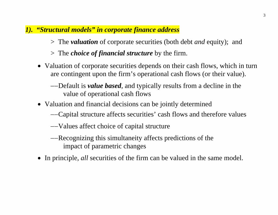
1). “Structural models” in corporate finance address

> The valuation of corporate securities (both debt and equity); and

> The choice of financial structure by the firm.

• Valuation of corporate securities depends on their cash flows, which in turn are contingent upon the firm’s operational cash flows (or their value).

−−Default is value based, and typically results from a decline in the value of operational cash flows

• Valuation and financial decisions can be jointly determined

−−Capital structure affects securities’ cash flows and therefore values

−−Values affect choice of capital structure

−−Recognizing this simultaneity affects predictions of the impact of parametric changes

• In principle, all securities of the firm can be valued in the same model.

4

2) Why structural models are important: −−Pricing debt, equity and other corporate securities Essential for buyers (investors), sellers (firms), and advisors

−−Εstimating default probabilities Useful to investors and policymakers The “Holy Grail” of bond ratings agencies?

−−Determining optimal capital structure decisions Essential for firms, but need for more precise guidance

−−Analyzing most corporate decisions that affects cash flows Determines value-maximizing decisions (e.g., investment)

−−Determining the impact of policy changes on firms’ values and decisions (e.g. effects of changes in Treasury rates, tax policies)

−−My talk is less ambitious! Focus on pricing, default risk, and capital structure

5

3) Topics to be covered LECTURE 1: Pros and Cons of Structural Models: An Introduction

a) A brief review of structural models in finance, and the “revolution”

following from Black and Scholes (1973) and Merton (1974)

b) A simple diffusion model incorporating finite debt maturity and endogenous

default

c) Empirical predictions of current structural models, and their shortcomings

−−The fundamental problem of diffusion models:

>> Underprediction of both credit spreads and default probabilities

for low risk debt and for shorter horizons.

>> This makes doubtful the wisdom of using current structural models

for recommendations about optimal capital structure

6

LECTURE 2: A New Structural Model

a) A structural model that answers most of these shortcomings

• Has a very simple jump-diffusion process for underlying cash flows

• Has a “liquidity” component of spreads in addition to default risk

• Has endogenous default

• Provides closed-form valuations for debt and equity −−Can readily compute credit spreads, default probabilities with Excel

• When calibrated to external data, the model matches historical credit spreads, default probabilities, and recovery rates quite accurately

b) Applications: quantitative estimates of optimal capital structure

• The model provides explicit (rather than general) advice on optimal leverage

• Can be used to examine the behavior of bond prices and optimal leverage

7

LECTURE 3: Financial Synergies and the Optimal Scope of the Firm Optimal firm scope: What should be the financial boundaries of a firm?

−−“Structured finance” has been an important recent development in financial markets, including

>> Asset securitization

>> Project finance

−−Yet financial theory has found structured finance difficult to explain, given the apparent absence of operational synergies.

−−We use a simple structural model to consider the purely financial synergies of mergers, spinoffs, or structured finance.

>> Financial factors that determine the optimality of separation vs. conglomeration are identified _____________________________ Caveats (the fine print): These lectures are a personal view, and time does not allow me to cover many issues in depth. I apologize in advance that numerous important contributions have been omitted. References cited infra. are provided at the end of Lecture 2.

8

Three Brief Observations: i) Structural models are often termed “credit risk” models. • They are now widely used by practitioners (e.g. Moody’s-KMV)

• They focus on debt valuation and default probabilities, taking financial structure as given (e.g. leverage, debt maturity)

• But structural models can go beyond debt pricing given financial structure

−−Used to analyze financial structure itself, including optimal leverage, maturity, risk hedging, and investment decisions.

• Changes in exogenous variables may affect firms’ financial decisions

−−Predictions of pricing and default models that ignore this feedback may be flawed.

9

ii) Structural models of credit risk are often contrasted with statistical or “Reduced form” (RF) models of estimating credit spreads and default probabilities.

• RF models assume default is not directly based on firms’ cash flows or values, but estimate a jump rate (intensity) to default empirically.

• RF models have been implemented widely, in part because their predictions of credit spreads seem more accurate than structural models--a problem I hope to redress in Lecture 2!

• RF models do not readily allow an integrated analysis of a firm’s decision to default or its optimal financial structure decisions

• David Lando’s book (Princeton, 2004) provides an excellent review of the reduced form approach, but this is outside the scope of my talk. Some recent models have combined the elements of both value-based default and jumps to default. I will mention these later.

10

iii) Most of my discussion will make simplistic but common assumptions

• Security types are given – debt and equity

−−no “optimal security design” issues

−−firms have a single type of debt (can be extended, but not here!)

• Markets are sufficiently complete to allow risk neutral valuation

• Shareholders seek to maximize the value of their shares

−−Rules out managerial conflicts or behavioral biases, −−But recognizes potential agency problems, e.g. vs. debt holders

• The firm’s operational cash flow is independent of financial structure

• Some papers have already started to relax the above assumptions (e.g. Leland (1998), Hackbarth (2005))

• I won’t be talking about correlation between defaults or the default behavior of bond portfolios. This remains an important topic.

11

I. A Brief Review

1) Modigliani-Miller (1958) Grandfather of structural models

• Uses simple model of valuation

−−No arbitrage (i.e. equal rates of return for equal risks) −−Riskfree debt

• With no taxes or default costs, total firm value is invariant to capital structure (i.e., no “optimal” capital structure).

2) The “tradeoff theory” of optimal capital structure introduced risky debt

• Optimal capital structure balances the tax benefits of debt with potential default costs

−−Stiglitz (1969), Kraus and Litzenberger (1973) state preference models

−−Provide important general insights, but little explicit guidance on either debt valuation or optimal leverage—preference based

12

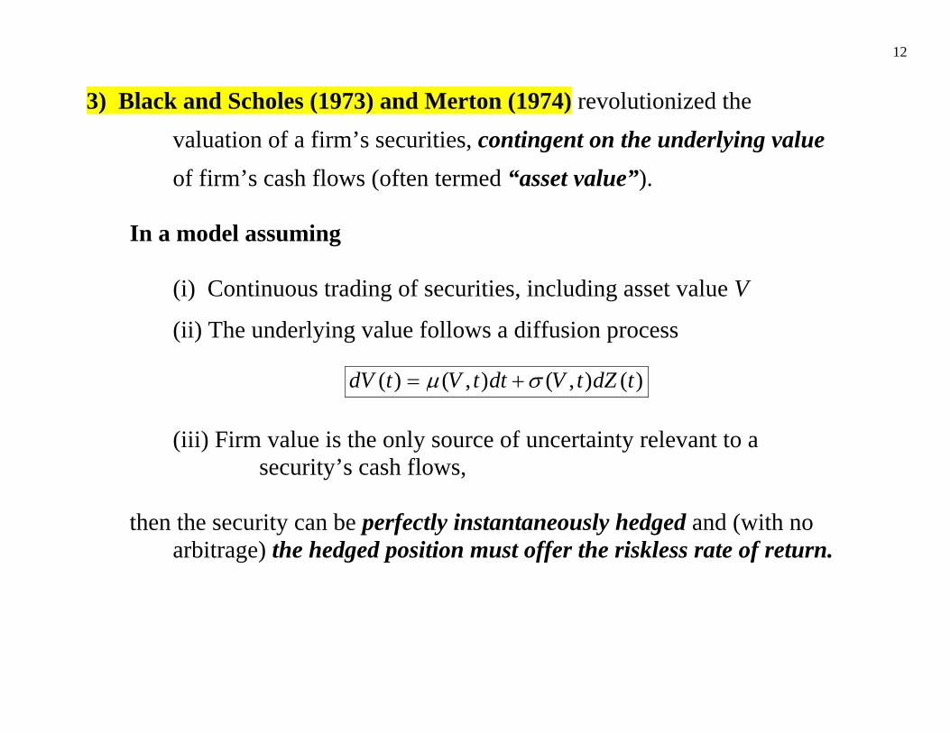
3) Black and Scholes (1973) and Merton (1974) revolutionized the

valuation of a firm’s securities, contingent on the underlying value

of firm’s cash flows (often termed “asset value”). In a model assuming (i) Continuous trading of securities, including asset value V

(ii) The underlying value follows a diffusion process

)(),(),()( tdZtVdttVtdV σμ += (iii) Firm value is the only source of uncertainty relevant to a security’s cash flows, then the security can be perfectly instantaneously hedged and (with no arbitrage) the hedged position must offer the riskless rate of return.

13

This in turn leads to the fundamental p.d.e.:

rGCFGGGCFrVG tVVV =++−+ )(5.0 2σ (1) (subscripts indicate partial derivatives, and arguments V and t of G, r, CF, and CFG are suppressed)* where CF is the total cash flow rate to all security holders, and CFG is the cash flow to the holders of the security whose value is G. > The p.d.e. (1), plus boundary conditions for the given security,

determine the valuation function G = G(V, t) ______________________________ *Note from Ito’s lemma that the l.h.s. of (1) is the expected total return of security G, when the underlying asset value V grows at expected rate rV - CF , i.e. the expected rate of return to asset V (including cash flow CF) is the riskfree rate r. The r.h.s. of (1) implies that the expected total rate of return to security G is also the riskfree rate r.

14

• The fact that the solution to (1) does not depend upon preferences

led Cox and Ross (1976) to RISK NEUTRAL VALUATION,

subsequently formalized by Harrison and Kreps (1979):

The value of a security equals its expected cash flows

discounted at the riskfree rate, when the underlying firm value

has a total expected return equal to the riskfree rate.

• The basic theory can be extended to allow multiple underlying

state variables, including interest rates, if markets are sufficiently

complete.

• If there are jumps in underlying firm value, risk neutral valuation

requires as many contingent claims be traded as possible jump levels.

15

4) The Merton (1974) and Black and Cox (1976) models

• Common Assumptions

−−Firm value follows a continuous time diffusion process.

−−Volatility σ and the riskfree rate r are constant over time

(“lognormal process”)

−− Net payout rate by the firm CF = 0

(Payouts to security holders financed by additional equity issuance)

−−There are no default costs or tax advantages to debt

(so no optimal capital structure – MM world)

• Merton model:

−−Zero-coupon debt, face value F, maturity T

−−Default only at T, iff V(T) < F

−−If default, bond holders get random V(T), equity holders gets zero

16

• Black & Cox model:

−−Perpetual debt (no principal repayment), constant coupon rate C

−−Default at any t, upon first passage of V(t) to default barrier VB

−−If default, bond holders get nonrandom VB, equity holders gets zero • Merton, B & C Shortcomings −−Don’t allow for debt that is coupon-paying and has finite maturity

−−Don’t allow analysis of optimal debt amount/maturity (capital structure)

without introduction of taxes, default costs

−−Have regularly-observed empirical difficulties:

>> Spreads too low for low-risk and low maturity debt

(Jones, Mason, & Rosenfeld (1984), others.)

17

• FINITE MATURITY DEBT, TAXES, AND DEFAULT COSTS

• Leland (1994b) and Leland & Toft ( LT, 1996) develop structural models

that include four additional aspects. *

−−Debt has average maturity T < ∞

−−Coupon interest is tax deductible

−−Default incurs default costs

−−The firm may have net cash payouts to security holders

• These extensions give the model considerably more flexibility and realism**

−−Allows closed-form determination of the term structure of credit spreads

−−Permits simple analysis of optimal capital structure ____________________________________ * Earlier models of Brennan & Schwartz (1978, 1984) and Mello & Parsons (1992) considered many of these aspects, but did not derive closed form solutions. ** Although (unlevered) asset value V may not be traded, trading of equity (or other contingent claim) allows use of V as the state variable (Ericsson & Reneby (2004))

18

Debt Value: Leland (1994b) Exponential Model (simpler than L&T 1996!)

• Same lognormal firm value process as Merton, Black & Cox.

• Cash flow paid out to security holders total δV, where δ is constant.

• Debt has total principal value P at time t = 0.

• The coupon rate on debt is C, chosen so that debt sells at par at t = 0

• Firm retires debt at a proportional rate m through time

…similar to a “sinking fund” (larger m shorter average life)

−−Debt outstanding at t = 0 has remaining principal value e −mt P at time t

−−Debt outstanding at t = 0 receives cash flow e −mt (C + mP) at t if

the firm remains solvent t.

−−In the absence of default, the average maturity of debt will be the time-weighted average

∫∞

− ==0

1)(m

dtmetT mt

19

• The firm replaces retired debt with new debt having the same principal

and coupon−−total P and C are constant (stationary capital structure). • Total debt service rate is C + mP = C + P/T (same as L&T 1996) • Tax benefits of debt have constant rate τ C while firm is solvent. • If default occurs at time t, debt outstanding at t = 0 has a claim on a

fraction e-mtP/P = e-mt of asset value after default costs,

i.e. a claim of value e-mt(1 – α)VB, where

>> VB is the (constant) boundary value triggering default and

>> α is the (constant) fraction of asset value lost in default. ______________________________ *It should be noted that the exponential model has already been used in several papers, including Leland (1998), Ericsson (1998), Ericsson, Reneby, & Wang (2005), Chen and Kou (2005), and Hackbarth, Miao, and Morellec (2006).

20

The value of debt: • We will derive debt value using risk neutral valuation, recalling

1) Discount expected cash flows at the riskfree rate r;

2) The expected rate of growth (“drift”) of firm value under the risk neutral measure is g ≡ r – δ .

>> Cash flows paid out* also grow at g.

3) Cash flows in solvency is e-mt (C + mP) at t, which are received with

probability 1 – F, where F = F(t; V0, VB) is the cumulative probability

function of the first passage time of V to VB, given V = V at t.

4) Cash flow from default at time t is e-mt (1 – α)VB, which occurs at t

with probability f = f(t; V0, VB), the density of the first passage time. __________________________ *A model with cash flows (rather than value) following a log Brownian motion is developed in Goldstein, Ju, and Leland (2001). With stationary parameters, firm value is a constant multiple 1/(r-g) of cash flows and results are essentially identical. Both approaches can be extended to include jump processes.

21

• The discounted expected value of debt’s cash flow under the risk

neutral probability measure is therefore

∫∫∞

−−∞

−− −+−+=00

)1()1()]([ dtfeeVdtFmPCeeD mtrtB

mtrt α (1)

Integrating the first term of (1) by parts gives

∫∫∞

+−∞

+− −+−++

=0

)(

0

)( )1()1( dtfeVdtfemrmPCD tmr

Btmr α

(2)

• We now use the only mathematical result we will need for the paper,

for lognormal processes with drift g and volatility σ :

22

The expected present value of $1 received at first passage to default VB

(from value V at t = 0), when discounted at an arbitrary rate z, is

2

5.02222

),(

0

00

)2)5.(()5.(),(

,),;(),(

σσσσ zggzgy

whereVVdtVVtfezgq

zgy

BB

zt

+−+−=

⎟⎟⎠

⎞⎜⎜⎝

⎛=≡

−∞−∫

(3)

NB: We have suppressed the other arguments of y and q. Using (3), the value of debt is

11

00

)1()1(

)1()1(11

qVqmrmPC

VVV

VV

mrmPCD

B

y

BB

y

B

α

α

−+−++

=

⎟⎟⎠

⎞⎜⎜⎝

⎛−+⎟⎟

⎠

⎞⎜⎜⎝

⎛−

++

=−−

(4)

where y1 = y(g, z) and q1 = q(g, z) in (3) when g = r – δ and z = r + m

23

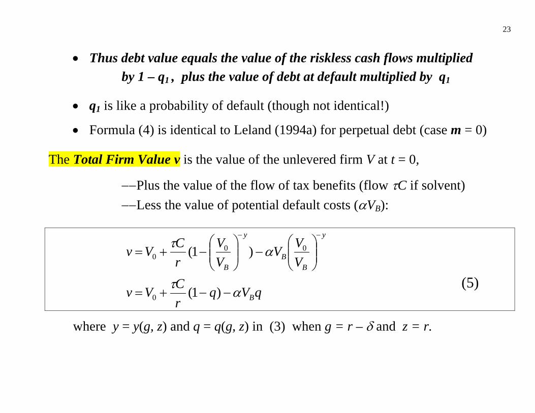
• Thus debt value equals the value of the riskless cash flows multiplied

by 1 – q1 , plus the value of debt at default multiplied by q1

• q1 is like a probability of default (though not identical!)

• Formula (4) is identical to Leland (1994a) for perpetual debt (case m = 0) The Total Firm Value v is the value of the unlevered firm V at t = 0,

−−Plus the value of the flow of tax benefits (flow τC if solvent)

−−Less the value of potential default costs (αVB):

qVq

rCVv

VVV

VV

rCVv

B

y

BB

y

B

ατ

ατ

−−+=

⎟⎟⎠

⎞⎜⎜⎝

⎛−⎟⎟

⎠

⎞⎜⎜⎝

⎛−+=

−−

)1(

)1(

0

000

(5)

where y = y(g, z) and q = q(g, z) in (3) when g = r – δ and z = r.

24

• The value of equity E is the total value less the value of debt

DvE −= (6) • Thus we have derived

Closed form results for D, E, and v, given default boundary VB

• Observation: As equations (1) – (6) are time independent, they also hold

for arbitrary starting time t and value V(t) ( ≥ VB)

• We still need to determine the default boundary VB, a topic that

we now address.

25

DEFAULT: Exogenous vs. Endogenous VB Three possible “triggers” of default have been proposed: First two (“exogenous”) do not depend on an equity value maximizing decision by shareholders – result from covenants or other exogenous constraints (i) Zero Net Worth trigger: Default when value V falls to P VB = P

(Brennan & Schwartz 1978, Longstaff & Schwartz 1995)

−− Could be triggered by a covenant triggering default if net worth becomes negative (V < P)

−− But firms often continue to operate with negative net worth.

−− Shareholder value typically will be positive at V = P. Would not default but issue more stock, pay coupon (dilution better than zero value)

−− Moody’s-KMV (Crosbie & Bohn 2003): VB = PShort + (1/2)PLong

26

(ii) Zero Cash Flow Trigger: when cash flow δV falls to C VB = C/δ

(Kim, Ramaswamy, & Sundaresan 1993)

−−But zero current net cash flow doesn’t always imply zero equity value

−−Shares typically have positive value at this VB. Would not default but pay coupon by issuing more stock (dilution better than zero value) (iii) Optimal Default (endogenous): VB maximizes equity value

(Black & Cox 1976, Mello & Parsons 1992, Leland 1994a)

−−Implies smooth-pasting condition: 0|);(=

∂∂

= BVVB

VVVE

• The optimal endogenous default barrier VB from (6) is:

yyr

yCmr

ymPC

VB αα

τ

+−+

−+

+

=1

1

)1(1)()(

(7)

27

Substituting (7) for VB in the formulas (4, 5, 6) for debt, firm, and equity

values gives closed form solutions for these values.

−−For bonds to sell at par, find coupon C that equates D(V0, C, P) = P. [Easy on Excel!]

• The Default Barrier and Comparative Statics

−−From (7), we can see that the endogenous default barrier VB depends on many of the model parameters (e.g. r, m, σ, α, δ)

−−With exogenous default, changes in maturity m, risk σ, the riskfree rate r, or default costs α don’t affect the level of VB.

−−A change in parameters will affect spreads and default probabilities differently, when the default barrier is endogenous vs. exogenous.

Example: σσσ ddV

VDD

ddD B

B∂∂

+∂∂

=

(second r.h.s. term = 0 when VB exogenous; ≠ 0 when VB, = 0 is exogenous)

28

To explore these questions, we need to

Calibrate the model to a reasonable set of parameters

• Period chosen: 1985-1995.

• Data to be matched is in Table 1

Huang & Huang (2003), Duffee (1998), and Elton & Gruber (2001)

–− Target spreads, recovery rates, leverage for Baa and B rated firms

–− Target default probabilities from Moody’s data, 1970-2000 . . .for comparison with Huang & Huang (2003) . . .data 1970-2005 not much different

• Plugging parameters for firms from Table 2 into the model generates

Figure 1 (predicted term structure of credit spreads) and

Figure 2 (predicted cumulative default probabilities)

29

Credit Spreads Targets SourcesHuang & Huang (HH, 2003), Duffee (1998), Elton & Gruber (EG, 2001)

A Rated 5 Yr. 90 bps HH: 96 Duffee: 87 EG: 7410 Yr. 100 bps HH: 123 Duffee: 96 EG: 7920 Yr. 115 bps HH: N/A Duffee: 117 EG: N/A

Baa Rated 5 Yr. 145 bps HH: 158 Duffee: 149 EG: 12110 Yr. 150 bps HH: 194 Duffee: 148 EG: 11820 Yr. 195 bps HH: N/A Duffee: 198 EG: N/A

B Rated 5 Yr. 470 bps HH: 470 (Based on Caouette, Altman, Narayanan (1998))10 Yr. 470 bps HH: 470 (Based on Caouette, Altman, Narayanan (1998))20 Yr. N/A

Riskfree Rate 8% HH: 8% (Average over period 1985-1995)

Default ProbabilitiesData: Moody's Special Comment 2001

A Rated Baa Rated B Rated 1 Yr. 0.01% 1 Yr. 0.14% 1 Yr. 6.16% 5 Yr. 0.54% 5 Yr. 1.82% 5 Yr. 27.90%10 Yr. 1.65% 10 Yr. 4.56% 10 Yr. 44.60%20 Yr. 4.79% 20 Yr. 11.27% 20 Yr. 54.20%

TABLE 1: TARGET SPREADS, DEFAULT DATA

30

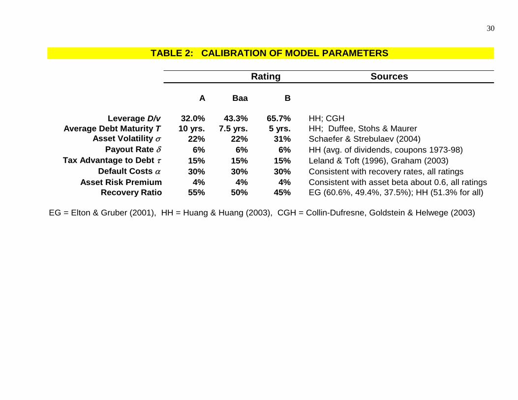
Rating Sources

A Baa B

Leverage D/v 32.0% 43.3% 65.7% HH; CGHAverage Debt Maturity T 10 yrs. 7.5 yrs. 5 yrs. HH; Duffee, Stohs & Maurer

Asset Volatility σ 22% 22% 31% Schaefer & Strebulaev (2004)Payout Rate δ 6% 6% 6% HH (avg. of dividends, coupons 1973-98)

Tax Advantage to Debt τ 15% 15% 15% Leland & Toft (1996), Graham (2003)Default Costs α 30% 30% 30% Consistent with recovery rates, all ratings

Asset Risk Premium 4% 4% 4% Consistent with asset beta about 0.6, all ratingsRecovery Ratio 55% 50% 45% EG (60.6%, 49.4%, 37.5%); HH (51.3% for all)

EG = Elton & Gruber (2001), HH = Huang & Huang (2003), CGH = Collin-Dufresne, Goldstein & Helwege (2003)

TABLE 2: CALIBRATION OF MODEL PARAMETERS

31

Notes: > We give somewhat greater weight to Duffee’s estimates of credit spreads, since he examines noncallable, coupon-paying bonds. Huang and Huang use Duffee’s data with minor modifications. > We choose Schaefer & Strebulaev’s (SS, 2004) estimates of asset volatility because they were derived from equity volatility data, and not chosen to generate default probabilities that matched data (as in HH’s approach). Thus, our approach allows model-predicted default probabilities to differ from historical probabilities. However, the SS volatility data comes from the period 1996-2002 and thus must be viewed as providing guidelines only. Prior to SS’s volatility estimates, Leland (2004) found that the L&T model fit the Moody’s default data best with volatilities of 23% (32%) for Baa-rated (B-rated) firms, very close to the SS estimates. > Although the model is flexible in all parameters, we assume that firms of different ratings differ only in terms of asset volatility, leverage, and maturity, for which data by ratings is available. While recovery data is also available (E&G) on a ratings basis, we find that when default costs α are kept constant (at 30%), the predicted recovery ratios across ratings vary and fit the target recovery ratios in Table 1 quite closely. > Asset betas, and therefore asset risk premia, may be higher for lower-rated firms. Lacking evidence, we assume no systematic risk changes across ratings for our analysis, although it would be straightforward to do so. It is also possible that debt maturity is shorter for lower-rated firms.

32

FIGURE 1 shows model fails to predict spreads of Baa-rated debt! About 1/3 of actual. . .

FIGURE 1 Term Structure of Credit Spreads - Baa-Rated Debt

Leland 1994 Exponential Model

0

50

100

150

200

0 5 10 15 20

Maturity (Yrs.)

Cre

dit S

prea

d

Duffee BaaElton-Gruber Baa22% vol.23% vol.

33

• Most empirical studies (EG, HH) confirm underestimates of spreads by structural models. • But Eom, Helwege and Huang (EHH, 2004) claim that L&T overestimates spreads— and substantially at short maturities.

−−This is very strange! For their parameters, quite similar to those in Table 1, I get substantial underestimates of spreads (both for L&T and exponential model)

−−I conclude that EHH implementation of L&T may be flawed.

• Possible explanation for underestimates of spreads by structural models:

MAYBE spreads reflect non-default factors, e.g. liquidity, state taxes (EG, HH)

−−But Leland (2004) notes that probabilities of default should

not be affected by these factors (in contrast with spreads)

−−Let’s see if model predicts default probabilities accurately

34

• FIGURE 2: Predicted probabilities of default.

FIGURE 2Cumulative Default Probability - Baa Rating7.5-Yr. Debt, Jump Intensity = 0.70%, k = .90

0.00%

2.00%

4.00%

6.00%

8.00%

10.00%

12.00%

14.00%

0 5 10 15 20

Years

Def

ault

Prob

abili

ty

Actual 1970-2005Model with 21.5% Vol.Model with 22.5% Vol.

35

• For longer horizons (t > 6 yrs.), observed default probabilities are bounded below

and above by the model’s predicted default rates for 21.5% and 22.5% volatilities.

(Recall estimate of Baa-rated firm volatility = 22%, Schaefer & Strebulaev). . . .Thus model does decently in predicting longer-horizon default rates . . .But predictions are far too low for short horizons for either volatility! (< 50% actual, t ≤ 4 yrs.)

• Observation: Low default predictions for short-term horizons (in contrast

with low predictions of spreads) cannot be rectified by nondefault factors • Many papers have suggested changes that could raise spreads,

while retaining a diffusion process for underlying firm value V: * ___________________________ * A list of references is provided at the end of Lecture 2.

36

1) Stochastic models of the default-free interest rate

Longstaff & Schwartz (LS, 1995) – Vasicek process

Kim, Ramaswamy, and Sundaresan (1993) – CIR process

Acharya & Carpenter (2002)

Notes: Including stochastic interest rates will lead to lower credit spreads if the correlation between interest rate and firm value processes is negative. Several studies find random rates have relatively small effects on spreads.

2) Strategic default, Renegotiation, Bank vs. public debt

Anderson & Sundaresan (1996)

Mella-Barral & Perraudin (1997), Mella-Barral (1999)

Fan & Sundaresan (2000)

Hackbarth, Hennessy, & Leland (2006)

Notes: Strategic default can raise credit spreads, but HH find the effect is empirically small when calibrated to historical default probabilities.

37

3) Bankruptcy: Absolute Priority not respected; Chapter 7 vs. 11

Leland (1994)

Francois & Morellec (2004)

Broadie, Chernov, & Sundaresan (2006)

4) Alternative Stochastic Processes (without jumps)

Collin-Dufresne & Goldstein (2001): mean reverting leverage ratios

Sarkar & Zapatero (2003): mean reverting cash flows

Leland (1998): risk hedging

Notes: Mean reversion typically imply lower spreads than random walk models. 5) Dynamic Capital Structure

Fischer, Heinkel, and Zechner (1989)

Goldstein, Ju, and Leland (2001)

Ju, Parrino, Peshman, and Weisbach (2005)

Ju & Ou-Yang (2005)

Notes: Dynamic models imply lower optimal leverage ratios than static models.

38

6) Endogenous Investment

Mauer and Triantis (1994)

Mauer and Ott (2000)

Childs, Mauer, and Ott (2005)

Hackbarth (2006) 7) Liquidity

Longstaff (1996)

Morellec (2001)

Ericsson (2006)

Notes: We take an alternative approach to liquidity premia in Lecture 2

• These models can imply reasonable credit spreads for longer maturities,

but all underestimate credit spreads and/or default risks for short horizons.

39

• The Problem: a pure diffusion process for firm value!

−−Spreads and default rates 0 as t 0. (e.g. Lando (2004), pp. 14-15). • This has led to using alternatives for structural models: >> Relating observed default probabilities to “Distance to default” (DD) measures using proprietary data (e.g., Moody’s-KMV)

. . . For high DD levels, this allows higher default likelihood than implied by a pure lognormal diffusion process.

>> Using reduced form models (“pure” jumps) • An Answer: Include jumps to default in structural models

−−This has been done previously (see literature review in Lecture 2),

but never with simple closed form solutions and endogenous default.

40

IN THE NEXT LECTURE:

• We introduce a simple jump-diffusion process

−−Provides closed form solutions with endogenous (diffusive) default

−−Explains default probabilities at short and long maturities

• But alas it does not fully explain credit spreads (short or long!)

• We then extend the model to include a liquidity premium to debt,

−−Can calibrate with data provided by Longstaff, Mithal, Neis (2004) and Ericsson, Reneby & Wang (2005).

• The extended model explains credit spreads as well as default probabilities

for both investment grade (A and Baa) debt and “junk” (B rated) debt.

−−Again, simple closed form solutions with endogenous default

−−The success of the model in these dimensions lends confidence to

using it to determine other corporate financial decisions

41

• Calibrating the model to the parameters in Tables 1 & 2, we consider

−−Optimal capital structure

−−Comparative statics of debt prices

• The model suggests that the −−Baa-rated firms (1985-1995) were close to their optimal leverage ratios.

−−A-rated firms were somewhat under-leveraged, whereas

−−B-rated firms were substantially over-leveraged, suggesting the sample

contains a substantial number of “fallen angels.”