structural optimization for effective strut-and-tie models · 2019-07-08 · structural...
TRANSCRIPT

Structural optimization for effectivestrut-and-tie modelsDesign of support crossbeams in single girderconcrete bridges
Master of Science Thesis in the Master Program Structural Engineering andBuilding Technology
SIMON NILSSONPETTER ÖHMAN
Department of Architecture and Civil EngineeringCHALMERS UNIVERSITY OF TECHNOLOGYMaster’s thesis ACEX30-19-77Gothenburg, Sweden 2019


Master’s thesis ACEX30-19-77
Structural optimization for effectivestrut-and-tie models
Design of support crossbeams in single girder concrete bridges
SIMON NILSSONPETTER ÖHMAN
Department of Architecture and Civil EngineeringDivision of Structural Engineering
Concrete StructuresChalmers University of Technology
Gothenburg, Sweden 2019

Structural optimization for effective strut-and-tie modelsDesign of support crossbeams in single girder concrete bridges
SIMON NILSSONPETTER ÖHMAN
© SIMON NILSSON, PETTER ÖHMAN, 2019.
Supervisors: Max Fredriksson, Inhouse TechAlexandre Mathern, Department of Architecture and Civil EngineeringMario Plos, Department of Civil and Environmental Engineering
Examiner: Mario Plos, Department of Civil and Environmental Engineering
Department of Architecture and Civil EngineeringDivision of Structural EngineeringConcrete StructuresChalmers University of TechnologySE-412 96 GothenburgTelephone +46 31 772 1000
Cover: 3D structural optimized crossbeam, optimized using BRIGADE/Plus Ver-sion 6.2-5 and Python 2.7, studied as a case study in the thesis.
Department of Architecture and Civil EngineeringGothenburg, Sweden 2019
iv

Structural optimization for effective strut-and-tie modelsDesign of support crossbeams in single girder concrete bridgesSIMON NILSSONPETTER ÖHMANDepartment of Architecture and Civil EngineeringChalmers University of Technology
AbstractThe strut and tie (ST) method is a method often used by structural engineers whenwhen designing reinforced concrete members with nonlinear stress flows. In bridgedesign, crossbeams for support by abutments is a typical example of a structurewhere the ST method often is applied. Experience from engineering practice indi-cates that the ST models used might be over-conservative, leading to an oversizedand costly reinforcement design. Therefore, there is a need to investigate if themethod and its applications can be improved and optimized.
The purpose of this master thesis was to investigate if structural optimization canbe used to find more effective ST models and thereby understand how today’s STmethod can be improved. This was achieved by performing a case study on acrossbeam in a bridge, previously designed by the civil engineering company InhouseTech AB.
The structural optimization method used in this thesis was a bi-directional evolu-tionary structural optimization (BESO). It was applied on the crossbeam using botha python-script, that was implemented in the Abaqus 6.14-2 extension BRIGADE/-Plus version 6.2-5, and a MATLAB-script. Both scripts are based on existingscripts, written by different authors, and implemented with a few modifications.For BRIGADE/Plus version 6.2-5, both 2D and 3D models were built, while theMATLAB-script only performed the optimization for the 2D case. The ST modelsobtained, based on the finite element (FE) analyses, were then assessed followingthe guidelines provided by Eurocode 2. These ST models was finally compared to a"conventional" ST analysis performed on the same crossbeam.
Several comparisons were made between different FE-analyses and hand calculationsto see which ST model led to the optimal way to design the reinforcement. It wasfound that in the models constructed with inclined ties the total reinforcementamount could be reduced.
Keywords: strut, tie, BESO, structural optimization, BRIGADE, Abaqus,Eurocode, crossbeam, finite element modelling, reinforcement design
v

Structural optimization for effective strut-and-tie modelsDesign of support crossbeams in single girder concrete bridgesSIMON NILSSONPETTER ÖHMANInstitution för arkitektur- och samhällsbyggnadsteknikChalmers tekniska högskola
SammanfattningStrut- and tie- (ST-) metoden används ofta av konstruktörer, vid dimensioneringav armering i konstruktionselement med icke-linjära spänningsflöden. Vid brokon-struktion är tvärbalkar vid stöd ett typiskt exempel på konstruktionselement påvilket ST-metoden ofta tillämpas. Yrkeserfarenheter visar att de ST-modeller somanvänds kan vara överkonservativa, vilket leder till en överdimensionerad och dyrarmeringsutformning. Därför är det nödvändigt att undersöka om metoden och dessapplikationerna kan förbättras och optimeras.
Syftet med detta examensarbete var att undersöka om strukturoptimering kan an-vändas för att hitta mer effektiva ST-modeller och därigenom förstå hur dagensST-metod kan förbättras. Detta uppnåddes genom att genomföra en fallstudie påen tvärbalk i en bro, tidigare konstruerad av konsultbolaget Inhouse Tech AB.
Strukturoptimeringsmetoden som användes i detta examensarbete var en så kallad"Bi-directional evolutionary structural optimization" (BESO). Den applicerades påtvärbalken genom att använda dels ett python-script, som implementerades i BRIGADE/Plus version 6.2-5, och dels ett MATLAB-script. Båda scripten är baserade påbefintliga script, skrivna av olika författare, och implementerade med några få mod-ifieringar. För BRIGADE/Plus version 6.2-5 byggdes både 2D- och 3D-modeller,medan MATLAB-scriptet endast utförde optimering för 2D-fallet. De erhållna ST-modellerna, som baserades på FE-analyserna, utvärderades sedan enligt riktlinjernafrån Eurocode 2. Slutligen jämfördes dessa ST-modeller med en "konventionell"ST-analys som utfördes på samma tvärbalk.
Flera jämförelser gjordes mellan olika FE-analyser och handberäkningar för att sevilken ST-modell som ger den optimala armeringsutformningen. Det visade sig attden totala mängden armering kunde minskas för ST modeller med lutande dragband.
Nyckelord: fackverksmodell, trycksträva, dragband, BESO, strukturoptimering,BRIGADE, Abaqus, Eurocode, tvärbalk, FE-modellering,dimensionering av armering
vi


PrefaceThis master thesis was conducted from January 2019 to June 2019, at the civil engi-neering company Inhouse Tech AB in Gothenburg. It is the final and conclusive workof the master of science program Structural Engineering and Building Technologyat Chalmers University of Technology.
We would like to extend our gratitude to our supervisors Max Fredriksson at InhouseTech AB, Alexandre Mathern at Chalmers University of Technology and Mario Plosat Chalmers University of Technology for the support through the project and toall the constructive feedback we have received.
We would also like to thank all the people working at Inhouse Tech AB for their hos-pitality and for taking their time discussing problems that arose during the project.
Finally we would like to thank our opponents Michaela Henriksson and Anna Ros-berg for their constructive feedback.
Simon Nilsson, Petter Öhman, Gothenburg, June 2019
viii


Contents
Abstract xii
Sammanfattning xii
Preface xii
Abbreviations xiii
Notations xiv
1 Introduction 11.1 Background . . . . . . . . . . . . . . . . . . . . . . . . . . . . . . . . 11.2 Aim and objectives . . . . . . . . . . . . . . . . . . . . . . . . . . . . 21.3 Limitations . . . . . . . . . . . . . . . . . . . . . . . . . . . . . . . . 21.4 Method . . . . . . . . . . . . . . . . . . . . . . . . . . . . . . . . . . 3
2 Theory 42.1 Discontinuity regions . . . . . . . . . . . . . . . . . . . . . . . . . . . 42.2 The Strut and tie method . . . . . . . . . . . . . . . . . . . . . . . . 5
2.2.1 The load path method . . . . . . . . . . . . . . . . . . . . . . 62.2.1.1 The development of a load path . . . . . . . . . . . . 62.2.1.2 Rules for the load path method . . . . . . . . . . . . 6
2.2.2 ST models developed from FE analyses . . . . . . . . . . . . . 72.2.3 ST method design according to Eurocode . . . . . . . . . . . . 7
2.2.3.1 Angles between struts and ties . . . . . . . . . . . . 72.2.3.2 Struts . . . . . . . . . . . . . . . . . . . . . . . . . . 82.2.3.3 Ties . . . . . . . . . . . . . . . . . . . . . . . . . . . 92.2.3.4 Nodes . . . . . . . . . . . . . . . . . . . . . . . . . . 9
2.2.4 Truss models for high beams . . . . . . . . . . . . . . . . . . . 102.2.4.1 Truss model with vertical ties . . . . . . . . . . . . . 112.2.4.2 Truss model with inclined ties . . . . . . . . . . . . . 11
2.3 Finite element method . . . . . . . . . . . . . . . . . . . . . . . . . . 112.3.1 The FEM in general . . . . . . . . . . . . . . . . . . . . . . . 112.3.2 FEM implementation in BRIGADE/Plus . . . . . . . . . . . . 12
2.4 Structural optimization . . . . . . . . . . . . . . . . . . . . . . . . . . 122.4.1 Mathematical form of structural optimization . . . . . . . . . 142.4.2 Different types of structural optimization . . . . . . . . . . . . 16
x

Contents
2.4.3 Bi-directional evolutionary structural optimization . . . . . . . 172.4.3.1 Optimization algorithm . . . . . . . . . . . . . . . . 182.4.3.2 Mesh dependency and convergence . . . . . . . . . . 20
2.5 Python . . . . . . . . . . . . . . . . . . . . . . . . . . . . . . . . . . . 202.6 MATLAB and CALFEM . . . . . . . . . . . . . . . . . . . . . . . . . 21
3 Case study and applied methods 223.1 Description of the studied beam . . . . . . . . . . . . . . . . . . . . . 233.2 Analytical development of Model A and B . . . . . . . . . . . . . . . 24
3.2.1 Development of Model A . . . . . . . . . . . . . . . . . . . . . 243.2.2 Development of Model B . . . . . . . . . . . . . . . . . . . . . 253.2.3 Verification of Model A using CALFEM . . . . . . . . . . . . 26
3.3 Development of Model C - 1 using structural optimization in MATLAB 263.3.1 Model C - 1 setup . . . . . . . . . . . . . . . . . . . . . . . . . 263.3.2 BESO implementation using MATLAB . . . . . . . . . . . . . 27
3.4 Development of Model C - 2 and Model C - 3 using structural opti-mization in BRIGADE/Plus . . . . . . . . . . . . . . . . . . . . . . . 283.4.1 Model C - 2 setup . . . . . . . . . . . . . . . . . . . . . . . . . 283.4.2 Model C - 3 setup . . . . . . . . . . . . . . . . . . . . . . . . . 293.4.3 BESO implementation using Python . . . . . . . . . . . . . . 31
3.4.3.1 Saving the filter map . . . . . . . . . . . . . . . . . . 333.4.3.2 Producing viewports . . . . . . . . . . . . . . . . . . 343.4.3.3 Verification of the python code . . . . . . . . . . . . 34
3.5 Development of Model C based on the sub-models . . . . . . . . . . . 353.5.1 Translation of the results from the sub-models . . . . . . . . . 353.5.2 The resulting Model C . . . . . . . . . . . . . . . . . . . . . . 36
3.6 Reinforcement design based on Model A, B and C . . . . . . . . . . . 37
4 Results 394.1 Results from Model A . . . . . . . . . . . . . . . . . . . . . . . . . . 39
4.1.1 Forces in struts and ties from Model A . . . . . . . . . . . . . 394.1.2 Verification of hand calculations for Model A using CALFEM 404.1.3 Check of critical nodes for Model A . . . . . . . . . . . . . . . 404.1.4 Reinforcement design for Model A . . . . . . . . . . . . . . . . 41
4.2 Results from Model B . . . . . . . . . . . . . . . . . . . . . . . . . . 424.2.1 Forces in struts and ties for Model B . . . . . . . . . . . . . . 424.2.2 Check of critical nodes for Model B . . . . . . . . . . . . . . . 424.2.3 Reinforcement design for Model B . . . . . . . . . . . . . . . . 43
4.3 Results from the sub models on which Model C are based . . . . . . . 444.3.1 Model C - 1 . . . . . . . . . . . . . . . . . . . . . . . . . . . . 444.3.2 Model C - 2 . . . . . . . . . . . . . . . . . . . . . . . . . . . . 464.3.3 Model C - 3 . . . . . . . . . . . . . . . . . . . . . . . . . . . . 47
4.4 Results from Model C . . . . . . . . . . . . . . . . . . . . . . . . . . 504.4.1 Forces in struts and ties from Model C . . . . . . . . . . . . . 504.4.2 Check of critical nodes for Model C . . . . . . . . . . . . . . . 504.4.3 Reinforcement design for Model C . . . . . . . . . . . . . . . . 51
, Architecture and Civil Engineering, Master’s Thesis ACEX30-19-77 xi

Contents
5 Discussion 525.1 Model A . . . . . . . . . . . . . . . . . . . . . . . . . . . . . . . . . . 525.2 Model B . . . . . . . . . . . . . . . . . . . . . . . . . . . . . . . . . . 535.3 Model C . . . . . . . . . . . . . . . . . . . . . . . . . . . . . . . . . . 53
5.3.1 Model C - 1 . . . . . . . . . . . . . . . . . . . . . . . . . . . . 545.3.2 Model C - 2 . . . . . . . . . . . . . . . . . . . . . . . . . . . . 545.3.3 Model C - 3 . . . . . . . . . . . . . . . . . . . . . . . . . . . . 545.3.4 Convergence of the sub-models . . . . . . . . . . . . . . . . . 55
5.4 Comparison between the models . . . . . . . . . . . . . . . . . . . . . 56
6 Conclusion 59
7 Further work 61
References 62
Appendix I
A Hand calculations IA.1 Hand calculations on Model A . . . . . . . . . . . . . . . . . . . . . . IA.2 Hand calculations on Model B . . . . . . . . . . . . . . . . . . . . . . XA.3 Hand calculations on Model C . . . . . . . . . . . . . . . . . . . . . . XIX
xii , Architecture and Civil Engineering, Master’s Thesis ACEX30-19-77

Abbreviations
2D Two dimensional3D Three dimensionalBESO Bi-directional evolutionary structural optimizationD-regions Discontinuity regionsESO Evolutionary structural optimizationFE Finite elementFEA Finite element analysisFEM Finite element methodIHT Inhouse Tech, civil engineering companym-script MATLAB scriptModel A The ST model obtained by using the ST method, as applied by Inhouse
Tech ABModel B The ST model obtained by using a different ST approach, were the ties
are placed with an inclination instead of vertical, as in Model AModel C The ST model are developed using structural optimization based on
different FE analysesPDE Partial differential equationsSIMP Solid isotropic material penalizationSLS Service limit stateST Strut and tieULS Ultimate limit state
xiii

Notations
Roman upper case letters
As Cross-sectional area of reinforcementC Objective function in BESO or compressive force in strutE0 Initial young’s modulusEe Artificial young’s modulusER Evolutionary ratioF Force vectorK(x) Stiffness matrixN Number of FE:s studied in homogenizationP External force in tiesR Reaction forceSO General form of structural optimizationT Tensile force in tieV Volume of design domainVf Volume fractionV k+1 Volume evolutionV s Upper volume limit in homogenization
Roman lower case letters
ae Width of a void in homogenizationbe Height of a void in homogenizationd Extension of a stressed region describing the extension of a disturbed regionf Objective function in general structural optimizationfcd Design compressive strength of concretefck Characteristic compressive strength of concretefyd Design yield strength of reinforcement steelh Highest part of a D-regionk0 Solid element stiffness matrixk1 National determined parameter governing CCC-nodesk2 National determined parameter governing CCT-nodesk3 National determined parameter governing CTT-nodesp Penalization factorrmin Filter radius
xiv

Contents
u Displacement vectorue Elemental displacement vectorve Elemental volumewi Weight factor used in structural optimizationxe Design variable in BESOx State variable in general structural optimizationy Design variable in general structural optimization
Greek letters
α Deviation angle for stresses under concentrated forcesαcc Coefficient considering long term effectsαth Sensitivity thresholdα̂ Mesh independent element sensitivityγc Partial factor for concrete in ordinary situationsν ′ National determined parameterΠ Potential energy in homogenizationθ1 Angle for strut meeting a single tieθ2 Angle for a strut between two perpendicular tiesθe Orientation of of the element in homogenizationρe Artificial element densityσRd,max Maximal compressive stress that a strut can carry
, Architecture and Civil Engineering, Master’s Thesis ACEX30-19-77 xv

Contents
xvi , Architecture and Civil Engineering, Master’s Thesis ACEX30-19-77

1Introduction
1.1 BackgroundThe Strut and tie (ST) method can be used to simulate the stress flow for discon-tinuity regions (D-regions) in reinforced concrete structures (Engström 2011). Thismethod is commonly used in today’s engineering practice. Experience indicates thatthe ST method is over-conservative1, particularly in cases with three dimensionalflow of forces (Mathern et al. 2017). One such case is crossbeams in bridge struc-tures. Figure 1.1a shows an example of how a bridge end support can be built upand in Figure 1.1b an describing sketch of a elevation view is visualized. The loadfrom the superstructure is transferred to the abutments by a crossbeam supportedon bearings.
(a) (b)
Figure 1.1: Visualization of the part of bridge studied in this thesis (a) Picture ofan end support in an existing bridge (b) Sketch of the assembly of the end support
Section A-A from Figure 1.1b, visualized in Figure 1.2, presents one example ofhow the ST method can be implemented on the crossbeam. The procedure fromthis stage is to calculate the forces in the ties and then design the reinforcementaccording to the capacity required.
1Max Fredriksson, Inhouse Tech AB
1

1. Introduction
Figure 1.2: Example of how the ST method can be implemented on crossbeams
An over-conservative method leads to an oversized and costly reinforcement design.Therefore, there is a reason to investigate if the ST method can be improved andoptimized, to be more efficient with respect to economy, environment and designand construction efficiency. One way to find an more effective ST model can be touse structural optimization.
The idea with structural optimization is to get a better understanding of how theforces flows within the structural element. Instead of guessing how the forces flowin loaded members, this optimization method can be used to get a more accuratepicture, and then the ST model can be developed according to the simulated flowof forces.
1.2 Aim and objectivesThe aim of this master thesis was to investigate the potential in using structuraloptimization to find effective ST models.
The main objectives of the study were to:• Perform a literature study regarding ST modelling and structural optimization.• Perform a case study where the knowledge obtained in the literature study is
applied on a crossbeam in an existing bridge.• From the case study obtain a ST model using the ST method and perform
calculations following the guidelines given by Eurocode.• From the case study obtain a ST model using structural optimization and
perform calculations following the guidelines given by Eurocode.• Compare the obtained ST models to see if the ST model obtained from struc-
tural optimization is more efficient than the ST model obtained from the con-ventional ST method.
1.3 Limitations• The crossbeam presented in the case study, with geometry and load cases, was
obtained from documentation at Inhouse Tech AB through supervisor MaxFredriksson.
• Only the reinforcement design of the crossbeam was investigated, even thoughthe ST method can be applied for other members of the bridge as well.
2 , Architecture and Civil Engineering, Master’s Thesis ACEX30-19-77

1. Introduction
• The difference in response due to different concrete and steel qualities was notinvestigated.
• The European standard (Eurocode 2 2008) was used during this project.• Only design methods for the ultimate limit state (ULS) were studied during
this project.
1.4 MethodLiterature studies were performed during the first half of the project. They provideddeeper understanding regarding design of D-regions, the ST method and how tointerpret Eurocode. They also provided new knowledge regarding different structuraloptimization methods, on which much of this thesis is based on. Some literaturewas provided by the research group (Concrete Structures) but most of it was foundby searches through the Chalmers library database and on the internet.
By using the ST method according to Eurocode 2 (2008)2 with vertical stirrups aST model was developed. This ST model served as a basis for comparison with theST models obtained from the FE analyses, on which structural optimization wasapplied.
FE analyses were conducted to obtain more efficient ST models. In those analyses,structural optimization theory was applied. A plugin script was developed, based onthe python script created by Zuo & Xie (2015), to be executed in the FE programBRIGADE/Plus version 6.2-5. In addition, a similar routine was implemented inMATLAB, to verify the ST models obtained by the BRIGADE/Plus simulations.This MATLAB-script (m-script) was written by Xia et al. (2016) and some minorchanges were done to make it suitable for this thesis purpose. The scripts performedstructural topology optimization and was used to obtain effective load paths, whichcould be translated into ST models.
The ST models, obtained from the structural topology optimization FE analyses,was checked to the requirements in Eurocode 2 (2008) and compared to the STmodel obtained from common ST methodology. Thus, it was possible to comparethe methods currently used in engineering practice to the developed optimized STmodels obtained by the FE analyses.
2as applied at Inhouse Tech AB
, Architecture and Civil Engineering, Master’s Thesis ACEX30-19-77 3

2Theory
2.1 Discontinuity regionsAs a result of geometric and/or static discontinuities, regular Bernoulli beam theorycan not be applied to certain regions of (concrete) structures, appearing in e.g.deep beams and corbels, Engström (2011). These regions are called disturbed- ordiscontinuity-regions, further referred to as D-regions. A D-region is characterizedby a non-linear stress distribution over the cross-section. These regions can bedescribed by Saint-Venant’s principle of body subjected to a system of forces inequilibrium. Saint-Venant stresses will appear as local effects in the body and will,according to Eurocode 2 (2008), be extended to d ≈ h where h is the highest partof the subjected section (see Figure 2.1).
Figure 2.1: Examples of different D-regions, based on Engström (2011)
According to Eurocode 2 (2008), a beam should be treated as a deep beam if thespan length is shorter than three times the overall section depth. For a deep beam,the stress and strain distribution becomes non-linear (see Figure 2.2) and the wholebeam can be considered as a D-region.
4

2. Theory
Figure 2.2: Normal strain distribution in a beam (top) vs. deep beam (bottom),based on Engström (2011)
2.2 The Strut and tie method
The strut and tie method (ST) is a lower bound approach used to simulate non-linear stress fields in D-regions (described in section 2.1) in ultimate limit state(ULS) in reinforced concrete. The ST method is based on the theory of utilizing thecompressive strength of concrete and adding reinforcement in tensile zones of thestructure. It is recommended that the ST models is based on the stress field underlinear elastic stress field (Engström 2011). The reason for this is that:
• The deformation capacity of concrete is limited by its ability of plastic rotation.• The requirements under SLS-loading should be fulfilled.
The ST method is suitable for reinforcement design in an early stage since the inputsneeded are few (Dahl 2018); geometry, load cases and concrete stiffness is enoughto get an appropriate model. The inputs needs to be combined using the followingassumptions:
• The stress field should be in equilibrium with the current load case.• No regions should be subjected to stresses above their plastic capacity.• The material should be assumed to be ideal plastic.
To develop an appropriate ST model based on linear elastic stress field, there aretwo main approaches:
• To use the load path method (Section 2.2.1).• To perform FE analyses from which the stress trajectories or principal stresses
can be used to develop an ST model (Section2.2.2).
, Architecture and Civil Engineering, Master’s Thesis ACEX30-19-77 5

2. Theory
2.2.1 The load path methodThe load path method can be used to simulate and simplify the stress field in deepbeams and other D-regions. This method is based on inserting single load path thatcorresponds to the flow of the stresses (Engström 2011).
For a simply supported deep beam, with uniformly distributed load, the shear forceis zero at mid-span. In this section, the load is divided so that half of the load goesto each support. This division of the loads creates a unique stress field which thenis translated to a unique load path from the applied load to the support. Thereare steps and rules to be followed in the load path method and this procedure willenables the development of a ST model.
2.2.1.1 The development of a load path
To achieve appropriate shape of the load path, Engström (2011) recommends toperform the following steps:
1. Identify the proportion of the load that goes to each support and where theload dividers are located.
2. Sketch the stress field.3. Use the resultant of the stress field in each section to sketch a smoothly curved
load path.4. If the load path is not able to characterize the shape of the stress field, the
load path is over-simplistic. Then the stress field has to be divided into moreparts.
5. Identify the transverse forces and their locations that is required to change thedirection of the load path in the D-region.
The simply supported beam studied in this thesis is considered as a deep beamwhere the whole beam is seen as a D-region. In such model, it is not possible tosketch a single smoothly curved load path, from the load to the support, due to theangle limitations stated in Eurocode 2 (2008). As step 4 in the list above suggest,the stress field has to be divided into more parts. This is done by using truss models(see section 2.2.4).
2.2.1.2 Rules for the load path method
There are rules and limitations to follow when using the load path method. En-gström (2011) describes them as:
• In each section, the load path should represent the resultant of the stress fieldwhich is simulated.
• Load paths can not cross each other.• The load path should start in the same direction as the applied load or support
reaction at the boundaries of the discontinuity region.• In the vicinity of a concentrated force, the load path should have a sharp bend.
6 , Architecture and Civil Engineering, Master’s Thesis ACEX30-19-77

2. Theory
• The load path should have a soft bend where it needs to change direction awayfrom a concentrated force.
2.2.2 ST models developed from FE analysesBy creating a FE model of the structure and performing linear FEA, principal stresstrajectories can be obtained to give an understanding of how the forces flow withinthe structure (Engström 2011). The trajectories can then be translated into strutsand ties to establish a ST model. By translating the stress flow in 2.3, a ST modelcan be developed.
Figure 2.3: Stress flow in a deep beam subjected to a distributed load acting onthe top of the beam
2.2.3 ST method design according to EurocodeIn Eurocode 2 (2008), guidelines is presented to how the ST method should be appliedand calculated. Additional guidelines are presented in Engström (2011) that governsthe recommendations of angles between the components of the ST model.
2.2.3.1 Angles between struts and ties
The angles between struts and ties should be taken into account during the designof the ST model (Mathern & Chantelot 2010). There are two reasons for this:
• Strain compatibility problems and a high need for plastic redistribution canarise if the deviation angle at concentrated forces is inappropriate.
• Strain compatibility problems can also arise if the angle between struts andties is too small.
The recommendations are summarized below, along with Figure 2.4, and are takenfrom Engström (2011), who are citing Schäfer (1999) in fib, Bulletin 2. In Figure
, Architecture and Civil Engineering, Master’s Thesis ACEX30-19-77 7

2. Theory
2.4, and throughout this report, the struts and ties are represented by dashed linesand solid lines respectively.
Figure 2.4: Angles to be taken into account in strut and tie design
• The angle θ1, for a strut meeting a single tie, should not be smaller than 45°.An angle of at least 60° is preferable.
• The angle θ2, for a strut between two perpendicular ties, should not be smallerthan 30°. An angle of at least 45° is preferable.
• The deviation angle α, for stresses under concentrated forces, should not ex-ceed 45°. A reasonable choice is α = 30°.
In addition to the rules regarding angle limitation, there is a rule saying that con-centrated forces in D-regions should not be carried by concentrated struts acrosswide elements (Engström 2011).
2.2.3.2 Struts
The multi axial state of stress, that a compressive strut experiences, influencesthe stress carrying capacity of the strut (Hendy C. R. & Smith D. A. 2007). Atransverse compressive stress will affect the capacity in a positive manner while atransverse tensile stress will affect the capacity negatively. Eurocode 2 (2008) givestwo simplified and conservative limits for the maximal compressive stress, σRd,max,that a strut can carry.
In case of no transverse stress or transverse compressive stress
σRd,max = fcd (2.1)
Here, fcd = αccfck
γcwith αcc = 0.85 and γc = 1.5. This expression will rarely be
possible to use since transverse tensile stress easily can occur.
In case of transverse tensile stress (cracked concrete)
8 , Architecture and Civil Engineering, Master’s Thesis ACEX30-19-77

2. Theory
σRd,max = 0.6ν ′fcd (2.2)
Here, fcd = fck
γcsince it is recommended that the factor αcc has the same value as
for shear design, i.e. αcc = 1. ν ′ is a parameter that is nationally determined and isrecommended to be ν ′ = 1− fck
250 with fck in MPa.
For compressive struts affected by transverse tensile stress, different limits for dif-ferent situations can be applied. These different situations can be quite difficultto distinguish. However, Equation 2.2 can be considered conservative for all thosesituations and was used in this thesis.
2.2.3.3 Ties
In a concrete structure, the forces in the tensile ties are carried by reinforcing steel.At the ULS, the reinforcement steel may be used up to its design yield strength(Hendy C. R. & Smith D. A. 2007). The center of gravity of the reinforcementbars should have the same position as the forces in the tensile ties. The requiredreinforcement cross-section area is given in Equation 2.3.
As = T
fyd(2.3)
Here, T is the tensile force in the tie and fyd is the design yield strength of thereinforcement steel.
The ties must also be adequately anchored at the nodes. For further reading regard-ing anchorage of ties, the reader is referred to Engström (2011).
2.2.3.4 Nodes
The intersections between struts and ties are known as nodes (Hendy C. R. & SmithD. A. 2007). A node can be seen as a volume of concrete and it is the geometryof connecting struts, ties and external forces that determines the dimensions of thenode.
There are two types of nodes (Engström 2011). One of those is the distributed node,which appears where distributed stress fields meets. They are never the criticalnodes, so there is no need to check those. The critical nodes that need to be checkedare the concentrated nodes, which appears where concentrated forces act.
The concentrated nodes should be designed with regard to the applied stresses atthe edges of the nodes (Engström 2011). There are several aspects that affects theseapplied stresses, e.g. dimensions of loading plates and bearings. The concentratednodes is divided into three different types, CCC-node, CCT-node and CTT-node,where C stands for compression strut and T for tensile tie. The maximum allowablestress, σRd.max, for each type of node is given below, according to Hendy C. R. &Smith D. A. (2007).
, Architecture and Civil Engineering, Master’s Thesis ACEX30-19-77 9

2. Theory
CCC-node
σRd,max = k1ν′fcd (2.4)
This node describes a node where all intersecting members are struts. The nationallydetermined parameter k1 is recommended to be 1.0 and ν ′ is defined in section2.2.3.2. This type of node does not typically occur in a truss model of a simplysupported beam with distributed load. It can occur at the compression faces offrame corners with closing moment and at internal beam supports.
CCT-node
σRd,max = k2ν′fcd (2.5)
This node describes a node where one intersecting members is a tie and the othersare struts. The nationally determined parameter k2 is recommended to be 0.85.This type of node can occur at e.g. end supports and in deep beams.
CTT-node
σRd,max = k3ν′fcd (2.6)
This node describes a node where two (or more) intersecting members are ties andthe others are struts. The nationally determined parameter k3 is recommended tobe 0.75.
Figure 2.5: Examples of node types, in a deep beam subjected to concentratedloads
2.2.4 Truss models for high beamsTo apply the ST method, a truss model for the structure or D-region, must bedeveloped. The truss model must fulfill the requirements on struts, ties, nodes andangles between struts and ties given in section 2.2.
In cases where the angles between the strut and the tie do not meet the requirementsstated in section 2.2.3.1, a simple strut and tie model can not be used (Engström2011). In such cases, a single load path can not be drawn from the load to the
10 , Architecture and Civil Engineering, Master’s Thesis ACEX30-19-77

2. Theory
support, so an other solutions have to be used. One way is to use a regular type ofthe ST method, known as "truss model".
2.2.4.1 Truss model with vertical ties
The idea with such model is to transfer the shear force, from the applied load to thesupport, by series of inclined compressive struts and vertical tensile ties (Engström2011). This enables distribution of stress fields so that the angle requirements canbe reached. The vertical ties will then act and have the same function as the shearforce reinforcement in a beam.
2.2.4.2 Truss model with inclined ties
For the construction worker, the handling of vertical stirrups are more convenientthan the handling of inclined stirrups1. This is one reason to why the use of inclinedstirrups is uncommon in design. However, inclined stirrups can be more effectivewhen it comes to carrying tension and thus reduce the needed amount of reinforcingsteel.
2.3 Finite element method
The finite element method (FEM) can be used to solve the often complex differ-ential equations that are encountered in engineering mechanics (Saabye Ottosen &Petersson 1992). In this section, the basics of the method is covered along with theimplementation of the method in BRIGADE/Plus.
2.3.1 The FEM in generalThe FEM is a numerical approach that leads to approximative solutions to generaldifferential equations. The differential equations, that describe a physical phenom-ena, are assumed to hold over a certain region (Saabye Ottosen & Petersson 1992).In the FEM, this certain region is divided into smaller sub regions (finite elements)for which the approximations are carried out in turn. This is a characteristic featureof the FEM which means that one approximation is not sought for the whole region.It is rather multiple approximations that are sought for the smaller sub regions.
As an example, let us assume that we have a problem where the variable varies ina non-linear manner over the entire region. Then, for the approximations over eachfinite element, it may be acceptable to assume that the variable varies in a linearmanner (Saabye Ottosen & Petersson 1992). When the behaviour of each elementhas been determined, the elements can be patched together following specific rules.Eventually, the behaviour of the entire region can be approximated.
1Rikard Migell, Inhouse Tech AB
, Architecture and Civil Engineering, Master’s Thesis ACEX30-19-77 11

2. Theory
In section 2.4, a method known as structural optimization will be described. Thismethod can for instance be used to find optimal solutions for structural problemsand are based on the finite element method.
2.3.2 FEM implementation in BRIGADE/PlusOver the past 20 years the rapid increase of computational power have made finiteelement (FE) simulations a powerful tool in structural engineering practice (Plevris& Tsiatas 2018). With the use of FE simulation programs such as e.g. BRIGADE/-Plus, a wide range of different simulations can be performed. These simulations cane.g. consist of static analyses, performed to find the load in ULS to non-linear anal-yses, which in turn are used to investigate the development of cracks in reinforcedconcrete (BRIGADE/Plus 6.2-5 2019).
In this thesis, BRIGADE/Plus version 6.2-5 was used to perform Bi-directionalevolutionary structural optimization (BESO). BRIGADE/Plus version 6.2-5 is anextension of Abaqus 6.14-2 and is customized to be used for structural engineer-ing purposes. BRIGADE/Plus consist of a toolbox with predefined loads andload combinations adapted to a wide range of design codes such as e.g. Eurocode(BRIGADE/Plus 6.2-5 2019).
2.4 Structural optimizationFor a given structural problem, structural optimization can be applied to find anoptimal solution to a given structural problem (Christiansen & Klarbring 2009).An optimal solution can be defined by different types of optimums. One can beto make a structure as light as possible, another to make a structure as stiff aspossible or to increase a structure’s resistance to buckling. In order to get welldefined optimums, different types of constraints need to be applied to the givenoptimization problem. Commonly used constraints in structural optimization arestresses, displacements and volumes. The measure of structural performance can bedefined as weight, stiffness, critical load, stress, displacements and geometry. Thesemeasures can then be used to define the objective function which is to be optimizedtowards its minimum or maximum.
Structural optimization is commonly divided into three methods: size/volume-,shape- and topology optimization. According to Christiansen & Klarbring (2009)the methods are based on:
• Size/volume optimization: The size or volume of members is changed to findthe most effective structure for a predefined given problem, this is visualizedin Figure 2.6.
12 , Architecture and Civil Engineering, Master’s Thesis ACEX30-19-77

2. Theory
Figure 2.6: Size optimization for a truss system, adapted from (Christiansen &Klarbring 2009). Reprinted with permission.
• Shape optimization: A design domain is described as sets of differential equa-tions. By integrating over the design domain a structure can be defined. Theoptimization can accordingly be defined by choosing the design domain forthe differential equations as effective as possible. No change of connectivityand no new boundaries can be created. An example of shape optimization ispresented in Figure 2.7.
Figure 2.7: Shape optimization of a structure defined by the function η(x), adaptedfrom (Christiansen & Klarbring 2009). Reprinted with permission.
• Topology optimization: The topology of the structure is allowed to change.This is done by removing or adding elements within the design domain of thestudied structure. This is made by allowing element areas or volume to be zeroor remaining fixed to a predefined size. Two types of topology optimization isvisualized in Figure 2.8.
, Architecture and Civil Engineering, Master’s Thesis ACEX30-19-77 13

2. Theory
(a)
(b)
Figure 2.8: Two types of topology optimization, adapted from (Christiansen &Klarbring 2009). (a) Topology optimization of a truss system. (b) Topology opti-mization by removing material from the structure. Reprinted with permission.
2.4.1 Mathematical form of structural optimizationIn Christiansen & Klarbring (2009) it is stated that for all structural optimizationproblems there is an objective function f that is used to classify the design andreturn a number to indicate progression of the optimization. f is usually chosen sothat a smaller number indicates a better optimization. Some examples of what fcan be measures of are effective stress, weight or displacements.
The state variable x describes a function or a vector that can be changed duringoptimization. In the common case x describes geometry or the choice of material.The design variable y is the output for a given x and describes the response of astructure in form of displacement, stress, strain or force (Christiansen & Klarbring2009).
By combining the objective function, state variable and design variable, the generalform of structural optimization (SO) can be stated as:
SO
minimize f(x, y) with respect to x and y
subject to
behavioral constraints on ydesign constraints on xequilibrium constraint
14 , Architecture and Civil Engineering, Master’s Thesis ACEX30-19-77

2. Theory
For a case with more than one objective function, so-called multiple criteria- orvector-optimization problems, the minimization problem is stated as followed:
minimize(f1(x, y), f2(x, y), ..., fl(x, y)) (2.7)
where l corresponds to the number of objective functions subjected to the sameconstraints as described for SO.
Since general structural optimization is not made for the same set of x and y, thereis no common case of solving the optimization for all fl. To deal with these typeof problems Pareto optimality is sought for. Pareto optimality means that no otherdesign satisfies the objectives better for x* and y* and no other x and y fulfill theconstraints(Christiansen & Klarbring 2009):
fi(x, y) ≤ fi(x∗, y∗) for all i = 1, ..., l (2.8)fi(x, y) < fi(x∗, y∗) for at least one i ∈ i = 1, ..., l (2.9)
One common way of finding Pareto optimal point is by introducing a weight factorwi ≥ 0 with i=1,...,l which satisfies ∑l
i=1 wi = 1 and yields the scalar objectivefunction:
l∑i=1
wi ∗ fi(x, y) (2.10)
The minimizing of Equation 2.10 under the constraints acting on SO can now besolved as a standard optimization problem with a Pareto optimal solution. It shouldbe noted that not all Pareto optimal points can be obtained by using Equation 2.10.
The objective function f is constrained in SO by three type of constraints,behavioral-, design- and equilibrium constraints(Christiansen & Klarbring 2009). Be-havioral constraints are constraints subjected to the state variable y. These con-straints can be expressed as g(y) ≤ 0 where g is a function describing e.g. displace-ments in a chosen direction. Design constraints governs the design variable x in asimilar way as behavioral constraints. These constraints can be combined to give acommon expression of g. Equilibrium constraints are based on the form:
K(x)u = F(x) (2.11)where K is the stiffness matrix, u the displacement vector and F is the force vec-tor. Here u takes the place of the state variable y. For continuum problems, theequilibrium constraints consists of partial differential equations (PDE). Treating thedesign variables, x and y, independently and provided that K can be inverted 2.11can be rewritten as, u(x) = K−1(x)F(x). Thus, the equilibrium constraint can beleft out and SO rewritten as (Christiansen & Klarbring 2009):
SO
min f(x,u(x))subject to g(x,u(x)) ≤ 0
(2.12)
, Architecture and Civil Engineering, Master’s Thesis ACEX30-19-77 15
2. Theory
This i called the nested formulation and can be used to solve structural optimizationproblems numerically. This is performed by deriving f and g with respect to thedesign variable x.
2.4.2 Different types of structural optimization
In engineering practice today, the ST method is a well defined rational methoddescribed in national design codes such as e.g. Eurocode. Using the guidelinesand rules described in chapter 2.2 it is up to each structural engineer’s engineeringjudgment to choose a ST model that satisfies the problem at hand. In cases withcomplex geometry and/or loading conditions this becomes a trial and error procedureto find a model that satisfies the codes. This model is sufficient to carry the load butis not assured to be an optima. According to Shobeiri & Ahmadi-Nedushan (2017)topology optimization can be used as an alternative approach to find optimal modelswhich can be translated into a ST model. In Qing Quan Liang et al. (2000) andOsvaldo M et al. (2017) several optimization procedures are presented.
The Homogenization method in Topology Optimization is described in Os-valdo M et al. (2017) as a method based on introducing micro voids within theelements of a given structure. These voids are then used as the design parametersin the optimization process. The optimization process is based on removing andadding material to expand or decrease the micro voids to create porous and solidregions. Therefore, the homogenization process can be seen as a type of TopologyOptimization which uses the micro voids to find optimal material parameters.
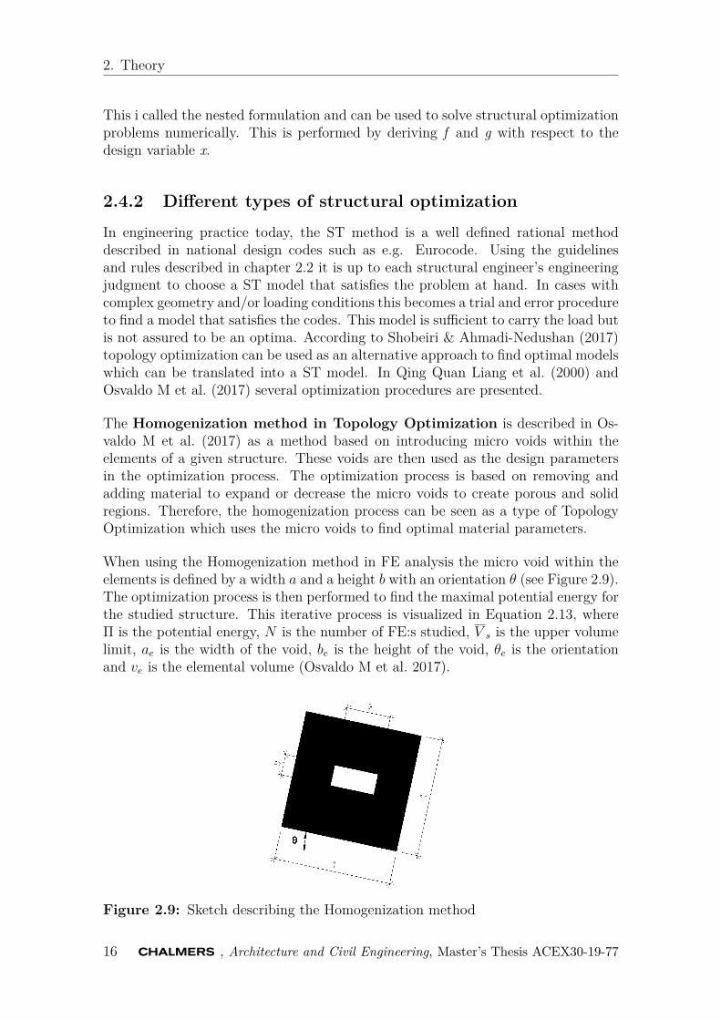
When using the Homogenization method in FE analysis the micro void within theelements is defined by a width a and a height b with an orientation θ (see Figure 2.9).The optimization process is then performed to find the maximal potential energy forthe studied structure. This iterative process is visualized in Equation 2.13, whereΠ is the potential energy, N is the number of FE:s studied, V s is the upper volumelimit, ae is the width of the void, be is the height of the void, θe is the orientationand ve is the elemental volume (Osvaldo M et al. 2017).
Figure 2.9: Sketch describing the Homogenization method
16 , Architecture and Civil Engineering, Master’s Thesis ACEX30-19-77

2. Theory
SO
Maximize: Π(u)
Subject to:N∑e=1
(1− aebe)ve − V s = 0
and
ae − 1 ≤ 0−ae ≤ 0be − 1 ≤ 0ae, be, θe = 1, 2, ..., N
(2.13)
Developed from the theory of homogenization, is the method of Solid IsotropicMaterial Penalization, further referred to as the SIMP-method. This methodis, according to Osvaldo M et al. (2017), the most renowned and most used incommercial software today. In this method an artificial element density ρe with avalue within the range 0 < ρmin ≤ ρe ≤ 1 is introduced. Multiplying the volumeof the element, ve, with the artificial element density produces the actual volume ofthe design domain as described in Equation 2.14.
V =N∑e=1
veρe (2.14)
A penalization factor, p, is introduced, which is applied to ρe when transforming theinitial young’s modulus E0 to artificial element young’s modulus Ee as described inEquation 2.15.
Ee = ρpeE0 (2.15)
The penalization factor p transforms the problem into a 0−1 problem. 0 is removedwhile 1 is kept for further iterations and to obtain a true optimization design valueof p > 3. The iterative SIMP process can thus be formulated as(Osvaldo M et al.2017):
SO
Maximize: c(pe)FTu
Subject to:N∑e=1
ρpeu = F
and
N∑e=1
veρe ≤ V s
0 < ρmin ≤ ρe ≤ 1e = 1, 2, ..., Np = 1, 2, ..., pmaxpmax > 3
(2.16)
2.4.3 Bi-directional evolutionary structural optimizationThe topology optimization routine that will be used in this thesis is the bi-directionalevolutionary structural optimization method, further referred to as the BESO-
, Architecture and Civil Engineering, Master’s Thesis ACEX30-19-77 17

2. Theory
method (Shobeiri & Ahmadi-Nedushan 2017). The BESO-method is a direct devel-opment of the evolutionary structural optimization method (ESO-method).
The ESO-method is based on removing ineffective materials from a structure inorder to find an optimal design (Shobeiri & Ahmadi-Nedushan 2017). In FE-designit can be translated to removing ineffective meshed elements while retaining theeffective elements. Since ESO removes elements based on initial criteria, the laterstages of the optimization can be affected by removing elements in early stageswhich can effect the final solution in a negative way.Through ESO, the improved
BESO-method has been developed (Shobeiri & Ahmadi-Nedushan 2017). BESOis based on the same theory of removing ineffective cells but also adding elementsnext to areas with high stresses. The BESO-method is more effective in terms ofcomputer efficiency in the iteration process and robustness of the final model thanthe ESO-method.
2.4.3.1 Optimization algorithm
By applying the BESO-method to the general optimization problem, the SO can,according to Zuo & Xie (2015), be stated as described in Equation 2.17.
SO
minimize C(X) = FTU = UTKU
subject to
X = {xe}, xe = 1 or xmin ∀ e = 1, ..., NF = KUV (X) =
∑X
xeve = V ∗
(2.17)
The BESO-method is a gradient based method where the design variable, also knownas the element sensitivity, αe is updated by differentiating the objective function Cwith respect to the design variable xe, described by Equation 2.18 (Zuo & Xie 2015).
αe = ∂C
∂xe(2.18)
The element sensitivity can be adapted from the SIMP-method using the materialmodel defined in Equation 2.19.
αe = −pxp−1e uTe k0ue = −p
xexpeuTe k0ue = −pEe
xe(2.19)
Where p is the penalty factor, that according to Equation 2.16, should be larger than3. uTe is the element displacement vector and k0 corresponds to the solid elementstiffness matrix with (xe = 1). xpuTe k0ue corresponds to the element strain energyEe which can be obtained using finite element analysis (FEA).
In order to obtain a mesh independent solution, the element sensitivity is updatedaccording to Equation 2.20 with weight function w(rej) according to Equation 2.21:
18 , Architecture and Civil Engineering, Master’s Thesis ACEX30-19-77

2. Theory
α̂ =∑j w(rej)αj∑j w(rej)
=∑j
w(rej)∑j w(rej)
αj =∑j
ηjαj (2.20)
w(rej) = max(0, rmin − rej) (2.21)
where the filter radius, rmin, is the smallest radius from the center of the i:th elementto the surrounding elements (see Figure 2.10). Using the filter radius, a filter mapcan be constructed which is used to calculate the sensitivities, i.e. the influence ofthe surrounding elements on the i:th element.
Figure 2.10: Description of the input rmin that is used to create the filter map
Convergence is reached by averaging the sensitivities calculated in Equation 2.20.This is done by averaging the current iteration with the previous iteration accordingto Equation 2.22.
α̃ = α̂ke + α̂k−1e
2 (2.22)
Starting with a full design the target volume for the next iteration is calculatedusing the evolutionary ratio, ER, as described in Equation 2.23 (Zuo & Xie 2015).By using the target volume, a threshold sensitivity αth is computed. This thresholdis used to determine which of the elements that should be assigned solid (αi > αth)and void (αi ≤ αth) element properties. This corresponds to assigning elements withelement sensitivities larger than the threshold with the design variable xmax = 1 andaccordingly smaller with xmin = 0.001. This value x for the elements then governsthe assignment of solid or void properties to the elements. Two types of approachescan be adopted hard- or softkill BESO. In hardkill BESO the stiffness of the voidelements are set to zero while in softkill BESO the stiffness of the element areassigned a low stiffness in order to obtain consistency in the optimization.
V k+1 = V k(1± ER) (2.23)
, Architecture and Civil Engineering, Master’s Thesis ACEX30-19-77 19

2. Theory
2.4.3.2 Mesh dependency and convergence
The BESO-method is mesh-dependent and this can cause problems for the finalresult (Xia et al. 2016). A more efficient topology design can always be obtained aslong as new holes are introduced in the design. This effect can be seen as a numericalinstability and there is a relation between a finer mesh and an increasing numberof holes. However, mesh-independent solutions can be obtained using BESO withperimeter control, see Equation 2.20 and 2.21 in section 2.4.3.1.
For a new design problem, it is not a trivial task to predict the value for the perimeterconstraint (Xia et al. 2016). The effect of using a too small value on the filter radius,rmin can be seen in Figure 2.11. The filter radius for the results shown in 2.11a and2.11b are set to 1 respectively 6 times the element length, and is the only inputthat differs in the two analyses. Figure 2.11a clearly shows a chess pattern that isundesired for the final design. According to Huang & Xie (2010) the filter radius iscommonly chosen as 2-3 times the size of the largest element.
(a) rmin = 1 (b) rmin = 6
Figure 2.11: Comparison between two analyses with different values on the filterradius. The two figures are extracted from FE analyses performed in MATLABduring this master thesis.
Even though the filter scheme, described with 2.20 and 2.21, is used, there can beproblems with convergence for the topology and the objective function (Xia et al.2016).
2.5 Python
Pyhton is a popular and commonly used programming language. It was createdand released by Guido van Rossum in 1991 and later developed by the PythonSoftware Foundation. The main emphasis of the Pyhton language is its readabilityand expressing its syntax in fewer lines of code (Saraswat n.d.).
20 , Architecture and Civil Engineering, Master’s Thesis ACEX30-19-77

2. Theory
2.6 MATLAB and CALFEMMATLAB is a computer program and program language developed by MathWorks.Its primary area of use is to perform mathemathical and technical calculations. Theprogram language is widely known in engineering practice.
During MATLAB’s existence, a vast number of toolboxes has been developed. Oneof those is CALFEM which is a toolbox containg finite element applications (Austrellet al. 2004).
, Architecture and Civil Engineering, Master’s Thesis ACEX30-19-77 21

3Case study and applied methods
This chapter will present a case study of improving a crossbeam in an existingbridge designed by Inhouse Tech AB. Firstly, the crossbeam studied is introduceddescribing the dimensions, loads and other properties of the beam. Secondly, thetwo analytical methods, in developing ST models, are described. Thereafter, theimplementation of structural optimization, using MATLAB and BRIGADE/Plus,to find effective ST models, are described. Finally, the translation from MATLABand BRIGADE/Plus results to ST models are presented.
For the reader to be able to follow this report more easily, names have been assignedto the different ST models:
• Model A - The ST model obtained by using the ST method, as applied byInhouse Tech AB.
• Model B - The ST model obtained by using a different ST approach, werethe ties are placed with an inclination instead of vertical, as in Model A.
• Model C - The ST model are developed using structural optimization basedon different FE analyses.
(a) Model A (b) Model B (c) Model C
Figure 3.1: Names of the different ST models
The development of Model C was carried out by optimizing finite element models.These FE models were created in MATLAB and BRIGADE/Plus. The sub-modelsstudied in order to obtain Model C was named as followed:
• Model C - 1: 2D model created in MATLAB.• Model C - 2: 2D model created in BRIGADE/Plus.• Model C - 3: 3D model created in BRIGADE/Plus.
Model C - 1 is described in section 3.3 while Model C - 2 and Model C - 3 aredescribed in section 3.4.
22

3. Case study and applied methods
3.1 Description of the studied beam
For the case study, a crossbeam from an existing Swedish road bridge was chosen.The bridge was originally designed by Inhouse Tech AB and is located in the middleparts of Sweden, just north of the lake Vättern. The geometry and dimensions ofthe crossbeam can be seen in Figure 3.2. In this figure, the coordinate system thatis used in this thesis, is also visualized. Note that only the span length of 4500 mmbetween the supports is included for the analyses of the developed ST models.
Figure 3.2: The geometry and dimensions of the beam studied in this thesis
There are several advantages to using this beam. Drawings and calculations fromthe existing bridge are available, revealing how it was designed and allowing forcomparisons. It also provides the opportunity to have an open dialogue with thedesigner of the bridge. In this way, calculations and assumptions, made in thisthesis, can be verified with experiences from today’s engineering practice.
As can be seen in Figure 3.2, the beam studied is not a deep beam according toEurocode 2 (2008), since the span length is larger than three times the height. How-ever, this structural element is part of a more comprehensive system and subjectedto 3D flow of forces. Therefore, as a simplification, the crossbeam is seen as a deepbeam with discontinuity regions where the ST method is applied.
For all calculations performed in this thesis, the distributed load q in Figure 3.2 isassumed to act at the bottom of the beam. In the real case, the major part of theload is transferred to the crossbeam from the main girder, connected to the side ofthe crossbeam. The load application is therefore distributed over its height. As asimplification, the assumption of load application to the bottom is made, to takethe need for lifting reinforcement into account. In the ST models, the load is furthersimplified as point loads, acting at the bottom of the crossbeam.
Both the concrete and steel class, together with the design loads, are obtained fromthe provided documents describing the calculations of the crossbeam. C35/45 isused for the concrete and K500C-T is used for the steel. The design load are set to6670 kN and are based on the total reaction for the bearings. This is the total force
, Architecture and Civil Engineering, Master’s Thesis ACEX30-19-77 23

3. Case study and applied methods
that should be lead through the beam down to the bearings. The dimensions of thebearings are 400x600 mm2.
3.2 Analytical development of Model A and BThe development of these two models was done in an analytical way, i.e. structuraloptimization was not implemented on these models. The two models were developedand then hand calculations were performed to calculate the forces in the struts andties. CALFEM was then used to verify the hand calculations. The two followingsubsections describes the development of Model A and B and presents the ST modelson which further calculations has been performed.
3.2.1 Development of Model AModel A is obtained by using the conventional ST method, following the guidelinesand recommendations given by Eurocode 2 (2008) and Engström (2011). Anotherproject was found in IHT’s database, were a similar crossbeam was designed usingconventional ST method. The calculations from that project were used as a basefor comparison with the calculation performed for Model A. Model A is visualizedin Figure 3.3 and the associated angles, point loads, reaction force and distances arepresented in Table 3.1. The labeling of struts, ties and nodes are also presented inthe figure. With these inputs, forces in the struts and ties were calculated and thecapacities of the nodes were checked according to the procedure described in Section2.2. These calculations and checks can be found in Appendix A.1.
Figure 3.3: Picture of the developed Model A, on which further calculations wereperformed
24 , Architecture and Civil Engineering, Master’s Thesis ACEX30-19-77
3. Case study and applied methods
Table 3.1: Distances, angles and forces associated with Model A
Distance [mm] Angle [°] Force [kN]A 498 y 58 R1 3 335B 584 x 32 P1 1 171C 584 w 58 P2 886D 584 v 32 P3 1 298d 1 050 s 58e 100 u 32h 1 200
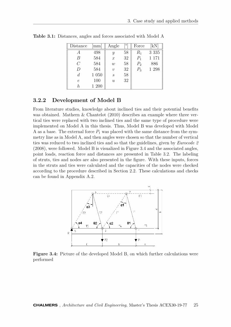
3.2.2 Development of Model BFrom literature studies, knowledge about inclined ties and their potential benefitswas obtained. Mathern & Chantelot (2010) describes an example where three ver-tical ties were replaced with two inclined ties and the same type of procedure wereimplemented on Model A in this thesis. Thus, Model B was developed with ModelA as a base. The external force P1 was placed with the same distance from the sym-metry line as in Model A, and then angles were chosen so that the number of verticalties was reduced to two inclined ties and so that the guidelines, given by Eurocode 2(2008), were followed. Model B is visualized in Figure 3.4 and the associated angles,point loads, reaction force and distances are presented in Table 3.2. The labelingof struts, ties and nodes are also presented in the figure. With these inputs, forcesin the struts and ties were calculated and the capacities of the nodes were checkedaccording to the procedure described in Section 2.2. These calculations and checkscan be found in Appendix A.2.
Figure 3.4: Picture of the developed Model B, on which further calculations wereperformed
, Architecture and Civil Engineering, Master’s Thesis ACEX30-19-77 25

3. Case study and applied methods
Table 3.2: Distances, angles and forces associated with Model B
Distance [mm] Angle [°] Force [kN]A 498 θ1 75 R1 3 335B 919 θ2 75 P1 1 916C 833 α1 35 P2 1 419d 1 050 α2 55e 100 α3 31h 1 200 α4 59
3.2.3 Verification of Model A using CALFEMThe hand calculations performed on the analytically developed Model A was verifiedby modelling the same problems in MATLAB. The toolbox CAFLEM was usedwhich made it possible to model the problem as a truss system in a simple way. TheFE analysis was implemented by using the CALFEM scripts bar2e.m, assem.m andsolveq.m.
3.3 Development of Model C - 1 using structuraloptimization in MATLAB
The development of sub-model Model C - 1 was carried out by using structuraloptimization in MATLAB. The resulting optimized FE model was then translatedinto a ST model. Here, the model setup for the FE analysis is described, followedby the implementation of BESO in MATLAB.
3.3.1 Model C - 1 setupThe structural optimization routine in MATLAB provided a less complex code andprocedure than the one for BRIGADE/Plus. The MATLAB script (m-script) usessquare plane stress elements and does only perform 2D-simulation. The mesh wascreated so that it reflected the dimensions of the studied deep beam, i.e. 450x120elements. Thus, each element was given an area of 1x1 cm2. To simulate distributedload on the bottom boundary, point loads was applied on all nodes on the bottomboundary, except the left- and rightmost node, see Figure 3.5. The properties ofthe mesh are presented in Table 3.3 and the inputs for the structural optimizationis presented in 3.4. These inputs was chosen, based on a number of performed trialsimulations.
26 , Architecture and Civil Engineering, Master’s Thesis ACEX30-19-77

3. Case study and applied methods
Figure 3.5: Model setup for the MATLAB script, describing mesh, applied loadand boundary conditions
Table 3.3: Inputs for the mesh for Model C - 1
Input ValueNumber of elements in x-direction [-] 450Number of elements in y-direction [-] 120
Total number of elements [-] 54 000
Table 3.4: Inputs for the structural optimization for Model C - 1
Input ValueVolume fraction, Vf [-] 0.45Filter radius, rmin [cm] 6
Evolutionary ratio, ER [-] 0.02
3.3.2 BESO implementation using MATLAB
The implementation of BESO in MATLAB was made to more easily investigate howthe different inputs (volume fraction, evolutionary rate and filter radius) effects theresulting model and to create sub-model Model C - 1, one of the sub-models on whichthe final Model C is based. From literature studies, a well written and explanatorym-script, written by Xia et al. (2016), was found. This m-script was used in thisthesis, with some modifications that will be described here. Even though hard-killBESO are implemented, the elements are not truly deleted. Instead, the elementsare assigned an very low Young’s modulus, similar to the case of soft-kill used inthe python code.
In this work, the script was modified so that the external load was applied as adistributed load on the bottom boundary of the beam and so that it produced thegraphs of the volume fraction and the objective function. The graphs were desiredto easily study the convergence of the analysis. Several lines were added to thescript, which can be seen in Figure 3.6 and Figure 3.7.
, Architecture and Civil Engineering, Master’s Thesis ACEX30-19-77 27

3. Case study and applied methods
Figure 3.6: Print screen of the used m-script. Line 20-28 was added to the scriptand line 39 was modified, to apply the load as a distributed load on the bottomboundary of the beam.
Figure 3.7: Print screen of the used m-script. Line 100-108 was added to plot thegraphs for the volume fraction and the objective function.
3.4 Development of Model C - 2 and Model C - 3using structural optimization in BRIGADE/-Plus
The development of sub-models Model C - 2 and Model C - 3 was carried outby using structural optimization in BRIGADE/Plus. The resulting optimized FEmodels was then translated into ST models. Here, the model setups for the FEanalyses is described, followed by the implementation of BESO in BRIGADE/Plus.In order to perform BESO in BRIGADE/Plus a Python script created by Zuo &Xie (2015) was used.
3.4.1 Model C - 2 setupThis subsection describes the different settings in the different modules in BRIGADE/-Plus and the inputs for the BESO routine for the setup for Model C - 2.
PartThe part was created defining the structural model to be a 2D plane stress model.
28 , Architecture and Civil Engineering, Master’s Thesis ACEX30-19-77

3. Case study and applied methods
Load• Load: The load was applied as a distributed load on the bottom edge of the
model, by using pressure load in the load module.• Boundary conditions: The boundary conditions was applied to the nodes in
the bottom corners of the model. The beam was modelled as simply supported.
MeshThe elements chosen for the 2D analysis was 8-node bi-quadratic plane stress quadri-lateral with reduced integration (CPS8R). The mesh size was implemented accordingto Table 3.5.
Table 3.5: Inputs for the mesh for Model C - 2
Input ValueNumber of elements in x-direction [-] 450Number of elements y-direction [-] 120
Total number of elements [-] 54000
Inputs for the BESO algorithmThe inputs Vf , rmin and ER, described in Section 2.4, needed to be chosen forthe optimization simulation. From trial simulations, it was found that the valuespresented in Table 3.6 gave satisfying results.
Table 3.6: Inputs for the structural optimization for Model C - 2
Input ValueVolume fraction, Vf [-] 0.35Filter radius, rmin [cm] 3
Evolutionary ratio, ER [-] 0.02
3.4.2 Model C - 3 setupThis subsection describes the different settings in the different modules in BRIGADE/-Plus and the inputs for the BESO routine for the setup for Model C - 3.Part
For the 3D case three parts was created.• Part-1 : Solid extrusion defining the body to be optimized.• Part-2 : Rigid plate defining the supports.• Part-3 : Planar shell to distribute the load.
InteractionTwo types of constraints was defined for the interaction between Part-1 and Part-3and between Part-2 and Part-3 respectively. For the interaction between Part-1 andPart-3 a tie constraint was defined, with Part-1 defined as the master surface andPart-2 defined as the slave surface. For Part-2 and Part-3, a rigid body constraint
, Architecture and Civil Engineering, Master’s Thesis ACEX30-19-77 29

3. Case study and applied methods
was defined. Part-2 defines the rigid body and was selected as the body element.A reference point was placed in the center of gravity of the plate. Part-3 waspartitioned so that the surface to be tied in the rigid body constraint correspondedto the size of Part-2.
When defining the tie constraint the following guidelines was followed (Vishark n.d.):
• The larger of the surface should act as the master surface.• The stiffer body should act as the master surface.• The part with the coarser mesh should act as master surface.
When defining the rigid body constraint the following was used (Defining rigid bodyconstraints 2017):
• Body elements will be defined by the elements of the rigid body.• A tie constraint will tie the deformable part to the rigid body.• A reference point needs to be defined, this point should preferably be placed
in the center of gravity of the rigid part. This point will govern the rotationof the part.
Load• Load: The load was defined as a pressure load action and applied on the part
of Part-3, between the supports, as visualized in Figure 3.2.• Boundary condition: The boundary conditions was defined in the reference
point of the rigid plate. In order to arrange the beam to work as a simplysupported beam the boundary condition is extended so that the beam onlycan rotate around the x-axis.
MeshFor Part-1, 8 nodal brick elements was assigned as element type and under ele-ment properties, reduced integration and enhanced hourglass control was applied(C3D8R). The reduced integration reduces the computational time required to runthe analysis and the enhanced hourglass control reduces the occurrence of hourglassing i.e. element distortion.
Choosing the mesh size was a somewhat heuristic process, but two guidelines wasestablished:
• The mesh should not be too coarse. A too coarse mesh leads to the risk ofsingle element rows, which easily rotates/distorts and affects the final solution.The mesh should also not be too fine since it leads to long computational time,as described in section 3.4.3.
• When the model contains different parts it is important that the slave surfacehas at least the same mesh size as the master surface. Thus, governs the sizeof Part-1 the size of Part-3’s mesh. Presented in Table 3.7 are the mesh sizeused in the optimization.
30 , Architecture and Civil Engineering, Master’s Thesis ACEX30-19-77

3. Case study and applied methods
Table 3.7: Inputs for the mesh for Model C - 3
Input ValueElement size in x-direction [-] 200Element size in y-direction [-] 40Element size in z-direction [-] 16Total number of elements [-] 128000
Inputs for the BESO algorithmThe inputs Vf , rmin and ER, described in Section 2.4, needed to be chosen forthe optimization simulation. From trial simulations, it was found that the valuespresented in Table 3.8 gave satisfying results.
Table 3.8: Inputs for the structural optimization for Model C - 3
Input ValueVolume fraction, Vf [-] 0.25Filter radius, rmin [cm] 30
Evolutionary ratio, ER [-] 0.02
3.4.3 BESO implementation using PythonIn this thesis, a general python code for BESO-optimization created and presentedin Zuo & Xie (2015), was used and modified. The code is implementing the BESO-algorithm presented in section 2.4.3 and subsection 2.4.3.1. The algorithm is dividedinto separate functions which then is called on by a main execution program. Inthis subsection these parts will be explained to give the reader a insight in how theBESO-algorithm can be implemented to perform topology optimization within aFEA-solver, in this case BRIGADE/Plus.
, Architecture and Civil Engineering, Master’s Thesis ACEX30-19-77 31

3. Case study and applied methods
The workflow of the code is visualized in Figure 3.8. The outline of the main pro-gram, executed as a script in BRIGADE/Plus, is that it calls on separate functionsto perform parts of the optimization. These different parts of the optimization isdescribed below.
Figure 3.8: Flowchart visualizing the BESO algorithm
The function fmtMdb prepares the model for the optimization routine. A solidmaterial is defined by creating an elastic material with the young’s modulus E = 1and Poisson’s ratio ν = 0.3. The python script implements the soft-kill BESOmethod and for the parts with a "void" material the properties are assigned toE = 1e−9 and Poisson’s ratio ν = 0.3. Two types of outputs is requested, one fieldoutput (ELEDEN ) corresponding the energy density equivalent to the element
32 , Architecture and Civil Engineering, Master’s Thesis ACEX30-19-77

3. Case study and applied methods
strains used when calculating element sensitivity’s. The second output is the historyoutput (ALLWK) stored as the external work. The external work can be visualizedas the compliance function C(x) which is the function to be minimized in Equation2.17. In the code, this corresponds to the objective function of the optimization andgoverns the development of the optimization.
The function preFlt creates the filter map, FM , which assures the mesh indepen-dence of the optimization. FM contains the influence of the surrounding elementswithin the distance rmin of each element’s center. This is computed by looping overall elements twice in order to obtain the influence of all elements.
Utilizing fmtMdb and preFlt, BESO is performed by creating a while loop governedby the function change corresponding to the convergence error of the objective func-tion of the optimization. As visualized in Figure 3.8, three steps are then executed:
• Perform FEA - uses the model defined in fmtMdb to perform linear-elasticanalysis to extract the elemental strain energy (ESEDEN ), which then isused to calculate the element sensitivity αe.
• fltAe: Filter sensitivity - applies the filtering scheme, created in preFlt, bymultiplying the raw sensitivities with the total weight factor ηj to obtain mesh-independent sensitivities as presented in Equation 2.20.
• BESO - By using the filtered sensitivities and target volume as inputs, thefunction BESO performs the main BESO routine. This routine is performedas described in section 2.4.3.1, by assigning the two variables lo and hi, corre-sponding to the largest and smallest filtered sensitivities. The target volume,tv, is calculated by multiplying the volume fraction with the initial volume ofthe solid elements described in 2.23 given as an input from the main program.Then, while (hi−lo)
hi> 1.0e − 5, a threshold th is calculated by averaging out
the sensitivities, which is used to update the convergence error change thatgoverns the optimization.
When the change criterion is false the while loop is terminated and the results issaved as Final_design.cae, which was used for post processing the results.
3.4.3.1 Saving the filter map
The filter mapping scheme, described in section 3.4.3 is created by looping overall the elements twice. This becomes a time consuming task to perform, as thenumber of loops increases quadratically with the number of elements. To reduce thecomputation time, the python library NumPy was deployed to decrease the need forarithmetic calculations.
The NumPy library is optimized for scientific computational calculations and treatsall entries within a list to decreases the time preparing the filter map FM (Zuo& Xie 2015). Thus, in order to avoid performing the filtering scheme every timethe code is executed, the code was modified to save the filter map as a pickle-file.Pickle is a python module that uses binary protocols for serializing and de-serializing
, Architecture and Civil Engineering, Master’s Thesis ACEX30-19-77 33
3. Case study and applied methods
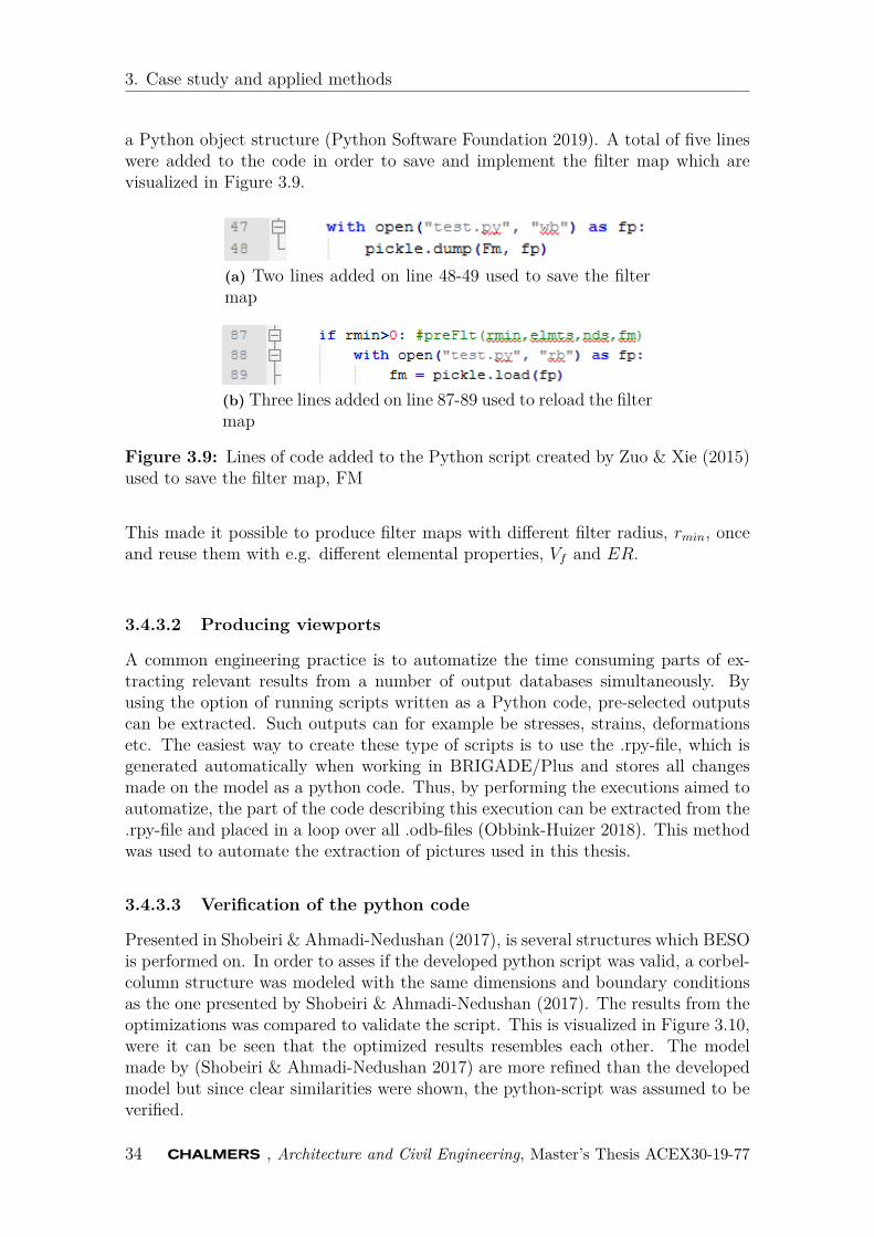
a Python object structure (Python Software Foundation 2019). A total of five lineswere added to the code in order to save and implement the filter map which arevisualized in Figure 3.9.
(a) Two lines added on line 48-49 used to save the filtermap
(b) Three lines added on line 87-89 used to reload the filtermap
Figure 3.9: Lines of code added to the Python script created by Zuo & Xie (2015)used to save the filter map, FM
This made it possible to produce filter maps with different filter radius, rmin, onceand reuse them with e.g. different elemental properties, Vf and ER.
3.4.3.2 Producing viewports
A common engineering practice is to automatize the time consuming parts of ex-tracting relevant results from a number of output databases simultaneously. Byusing the option of running scripts written as a Python code, pre-selected outputscan be extracted. Such outputs can for example be stresses, strains, deformationsetc. The easiest way to create these type of scripts is to use the .rpy-file, which isgenerated automatically when working in BRIGADE/Plus and stores all changesmade on the model as a python code. Thus, by performing the executions aimed toautomatize, the part of the code describing this execution can be extracted from the.rpy-file and placed in a loop over all .odb-files (Obbink-Huizer 2018). This methodwas used to automate the extraction of pictures used in this thesis.
3.4.3.3 Verification of the python code
Presented in Shobeiri & Ahmadi-Nedushan (2017), is several structures which BESOis performed on. In order to asses if the developed python script was valid, a corbel-column structure was modeled with the same dimensions and boundary conditionsas the one presented by Shobeiri & Ahmadi-Nedushan (2017). The results from theoptimizations was compared to validate the script. This is visualized in Figure 3.10,were it can be seen that the optimized results resembles each other. The modelmade by (Shobeiri & Ahmadi-Nedushan 2017) are more refined than the developedmodel but since clear similarities were shown, the python-script was assumed to beverified.
34 , Architecture and Civil Engineering, Master’s Thesis ACEX30-19-77

3. Case study and applied methods
(a) (b) (c)
Figure 3.10: Optimization of a corbel structure made to verify the python codeused. (a) Optimization made in Shobeiri & Ahmadi-Nedushan (2017). Reprintedwith permisson. (b) Optimization made to verify the python code, 2D visualization.(c) Optimization made to verify the python code, 3D visualization.
3.5 Development of Model C based on the sub-models
To be able to perform hand calculations on the obtained optimized sub-models, thesub-models had to be translated into ST models along with relevant angles anddistances. This section describes how the three sub-models were combined into onefinal Model C.
3.5.1 Translation of the results from the sub-models
The results from the FE analyses were translated and interpreted using AutoCAD.Pictures of the optimized models was extracted from BRIGADE/Plus and MATLABand then imported in AutoCAD. Then the lines were drawn after the existing strutsand ties. The next step was to measure the relevant angles and distances neededfor the hand calculations. Those quantities was easily measured in AutoCAD andeventually this procedure lead to an computable ST model.
As mentioned in the introduction to this chapter, Model C was developed based onthe results of the three different sub-models from the FE analyses. The procedureis visualized in Figure 3.11. The ST models from the different FE analyses wascombined and placed over each other, and then the final Model C was drawn afterthis combination.
, Architecture and Civil Engineering, Master’s Thesis ACEX30-19-77 35

3. Case study and applied methods
Figure 3.11: Picture describing how the sub-models were combined into the finalModel C
3.5.2 The resulting Model C
Model C is visualized in Figure 3.12 and the associated angles, forces and distancesare are presented in Table 3.9. The calculations performed for Model A can be foundin Appendix A.3. Note that all the angles between the struts and ties are presenteddirectly in Figure 3.12.
Table 3.9: Distances, angles and forces associated with Model C
Distance [mm] Angle [°] Force [kN]A 321 θ1 59 R1 3 335B 268 θ2 50 P1 674C 386 θ3 50 P2 485D 405 θ4 45 P3 586E 376 θ5 45 P4 579F 494 P5 1 011d 1 050e 104h 1 200
36 , Architecture and Civil Engineering, Master’s Thesis ACEX30-19-77
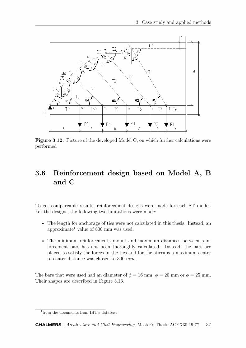
3. Case study and applied methods
Figure 3.12: Picture of the developed Model C, on which further calculations wereperformed
3.6 Reinforcement design based on Model A, Band C
To get compareable results, reinforcement designs were made for each ST model.For the designs, the following two limitations were made:
• The length for anchorage of ties were not calculated in this thesis. Instead, anapproximate1 value of 800 mm was used.
• The minimum reinforcement amount and maximum distances between rein-forcement bars has not been thoroughly calculated. Instead, the bars areplaced to satisfy the forces in the ties and for the stirrups a maximum centerto center distance was chosen to 300 mm.
The bars that were used had an diameter of φ = 16 mm, φ = 20 mm or φ = 25 mm.Their shapes are described in Figure 3.13.
1from the documents from IHT’s database
, Architecture and Civil Engineering, Master’s Thesis ACEX30-19-77 37

3. Case study and applied methods
Figure 3.13: Shapes of the reinforcement bars used in this thesis
38 , Architecture and Civil Engineering, Master’s Thesis ACEX30-19-77

4Results
This chapter presents the results from the different analyses and ST models. Firstly,the results for Model A and B are presented, which both do not include any struc-tural optimization. Secondly the results from the sub-models to Model C are pre-sented and finally the results for Model C.
4.1 Results from Model AIn this section, the results from Model A are presented, in terms of forces in strutsand ties, checks of critical nodes and the final reinforcement design.
4.1.1 Forces in struts and ties from Model AThe locations and labeling of struts, ties, nodes and external and reaction forces arepresented in Figure 4.1 and the associated magnitudes are presented in Table 4.1.
Figure 4.1: Locations of struts, ties, nodes and external and reaction forces forModel A
39

4. Results
Table 4.1: Normal forces in struts and ties together with external and reactionforces for Model A
Strut [kN] Tie [kN] Point loads and reaction force [kN]C1 1 375 T1 1 171 R1 3 335C2 2 391 T2 2 037 P1 1 171C3 3 915 T3 3 335 P2 866C4 4 022 T4 4 022 P3 1 298C5 3 302 T5 4 022C6 2 050 T6 3 302
T7 2 050
4.1.2 Verification of hand calculations for Model A usingCALFEM
The results from the FE analysis in CALFEM are presented in Table 4.2. Theycorrespond very well with the values in Table 4.1 and thus confirm the correctnessof the hand calculations.
Table 4.2: Normal forces in struts and ties from the results of FE analysis inCALFEM for Model A
Strut [kN] Tie [kN]C1 1 375 T1 1 171C2 2 391 T2 2 037C3 3 914 T3 3 335C4 4 023 T4 4 022C5 3 302 T5 4 022C6 2 050 T6 3 302
T7 2 050
4.1.3 Check of critical nodes for Model ANode 2 and 7 in Figure 4.1 are the critical nodes in Model A and are checked againstthe requirements given by Eurocode 2 (2008). The results are presented in Table4.3. The first index, in the node columns, stands for node number and the last onefor which force that is used for the check.
Table 4.3: Checks according to requirements from Eurocode 2 (2008) for Model A
Maximal stress Node 2 Node 7σRd.max 17.1 MPa σ2.C4 13.0 MPa σ7.R1 13.9 MPa
σ7.C3 13.1 MPa
40 , Architecture and Civil Engineering, Master’s Thesis ACEX30-19-77

4. Results
4.1.4 Reinforcement design for Model AThe reinforcement design for Model A is presented in Figure 4.2. The volume ofthe reinforcement, that corresponds to this design, and its ratio to the amount ofconcrete is presented in Table 4.4.
Common for all final reinforcement designs, Figure 4.2, 4.4 and 4.16, is that theyall have the same amount of minimum reinforcement. The bars marked with "MIN.REIN." in the above stated figures, are thus not included in the calculations for thevolumes of reinforcement.
Figure 4.2: Reinforcement design for Model A
Table 4.4: The volume of the reinforcement used for the reinforcement design ofModel A
Stirrups [m3] 0.087Horizontal bars [m3] 0.085
Total reinforcement [m3] 0.172Concrete [m3] 14.880Volume ratio [-] 0.012
Mass to volume ratio [kg/m3] 90.161
, Architecture and Civil Engineering, Master’s Thesis ACEX30-19-77 41

4. Results
4.2 Results from Model BIn this section, the results from Model B are presented, in terms of forces in strutsand ties, checks of critical nodes and the final reinforcement design.
4.2.1 Forces in struts and ties for Model BThe locations and labeling of struts, ties, nodes and external and reaction forces arepresented in Figure 4.3 and the associated magnitudes are presented in Table 4.5.
Figure 4.3: Locations of struts, ties, nodes and external and reaction forces forModel B
Table 4.5: Normal forces in struts and ties together with external and reactionforces for Model B
Strut [kN] Tie [kN] Point loads and reaction force [kN]C1 2 339 T1 1 983 R1 3 335C2 3 891 T2 3 453 P1 1 916C3 4 752 T3 4 752 P2 1 419C4 2 897 T4 4 239
T5 2 004
4.2.2 Check of critical nodes for Model BNode 2 and 5 in Figure 4.3 are the critical nodes in Model B and are checked againstthe requirements given by Eurocode 2 (2008). The results are presented in Table4.6. The first index, in the node columns, stands for node number and the last onefor which force that is used for the check.
42 , Architecture and Civil Engineering, Master’s Thesis ACEX30-19-77

4. Results
Table 4.6: Checks according to requirements from Eurocode 2 (2008) for Model B
Maximal stress Node 2 Node 5σRd.max 17.1 MPa σ2.C3 15.3 MPa σ7.R1 13.9 MPa
σ7.C2 13.0 MPa
4.2.3 Reinforcement design for Model BThe reinforcement design for Model B is presented in Figure 4.4. The volume ofthe reinforcement, that corresponds to this design, and its ratio to the amount ofconcrete is presented in Table 4.7. The volume from "Inclined bars", in Table 4.7,represents the volume for a part of the bars named J, in Figure 4.4. They arecalculated from the point where the bars leave the bottom layer till the point wherethey are anchored, 800 mm behind the nodes. Thus, the bottom part of the J-barsare included in "Horizontal bars" in Table 4.7 (see Figure 4.5).
Figure 4.4: Reinforcement design for Model B
Figure 4.5: Description of how the J-bars are divided into "Horizontal bars" and"Inclined bars" in Table 4.7 and Table 4.10
, Architecture and Civil Engineering, Master’s Thesis ACEX30-19-77 43

4. Results
Table 4.7: The volume of the reinforcement used for the reinforcement design ofModel B
Inclined bars [m3] 0.047Stirrups [m3] 0.039
Horizontal bars [m3] 0.083Total reinforcement [m3] 0.169
Concrete [m3] 14.880Volume ratio [-] 0.011
Mass to volume ratio [kg/m3] 88.589
4.3 Results from the sub models on which ModelC are based
In this section the results from the optimization of Model C - 1, Model C - 2 andModel C - 3 will be presented. The calculations of the developed final Model C willbe presented in section 4.4.
4.3.1 Model C - 1The development of the structural optimization for Model C - 1, which was per-formed in MATLAB, can be seen in Figure 4.6. Here, three of the 49 iterations arevisualized. Figure 4.7 visualises the corresponding graphs for the objective functionand volume fraction. Iteration 49 is the last iteration from this analysis and theresulting model from this iteration was further analyzed.
(a) Iteration 3
(b) Iteration 20
(c) Iteration 49
Figure 4.6: The development of the structural optimization for Model C - 1
44 , Architecture and Civil Engineering, Master’s Thesis ACEX30-19-77

4. Results
(a) Objective function (b) Volume fraction
Figure 4.7: Corresponding graphs for the objective function and the volume frac-tion for the final design of sub-model Model C - 1. Graphs created in MATLAB.
The angles and relevant lengths for the ST model, that comes out of the 49:thiteration of the FE analysis, are visualized in Figure 4.8. This ST model contributesto the final design of Model C.
Figure 4.8: The angles and relevant lengths for the ST model that comes out ofModel C - 1
, Architecture and Civil Engineering, Master’s Thesis ACEX30-19-77 45

4. Results
4.3.2 Model C - 2The development of the structural optimization for Model C - 2, which was per-formed in BRIGADE/Plus, can be seen in Figure 4.9. Here, three of the 60 itera-tions are visualized. Figure 4.10 visualizes the corresponding graphs for the objectivefunction and volume fraction. Iteration 60 is the last iteration for this analysis andthe resulting model from this iteration was further analyzed.
(a) Iteration 10
(b) Iteration 40
(c) Iteration 60
Figure 4.9: The development of the structural optimization for Model C - 2
46 , Architecture and Civil Engineering, Master’s Thesis ACEX30-19-77

4. Results
(a) Objective function
(b) Volume fraction
Figure 4.10: Corresponding graphs for the objective function and the volume frac-tion for the final design of sub-model Model C - 2. Graphs created in BRIGADE/-Plus.
The angles and relevant lengths for the ST model, that comes out of the 60:thiteration of the FE analysis, are visualized in Figure 4.11. This ST model contributesto the final design of Model C.
Figure 4.11: The angles and relevant lengths for the ST model that comes out ofModel C - 2
4.3.3 Model C - 3The development of the structural optimization for Model C - 3, which was per-formed in BRIGADE/Plus, can be seen in Figure 4.12. Here, three of the 78 itera-
, Architecture and Civil Engineering, Master’s Thesis ACEX30-19-77 47
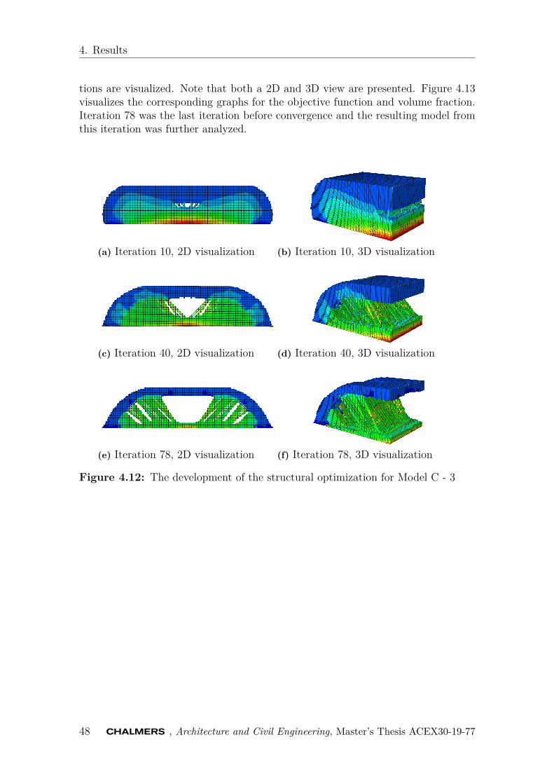
4. Results
tions are visualized. Note that both a 2D and 3D view are presented. Figure 4.13visualizes the corresponding graphs for the objective function and volume fraction.Iteration 78 was the last iteration before convergence and the resulting model fromthis iteration was further analyzed.
(a) Iteration 10, 2D visualization (b) Iteration 10, 3D visualization
(c) Iteration 40, 2D visualization (d) Iteration 40, 3D visualization
(e) Iteration 78, 2D visualization (f) Iteration 78, 3D visualization
Figure 4.12: The development of the structural optimization for Model C - 3
48 , Architecture and Civil Engineering, Master’s Thesis ACEX30-19-77
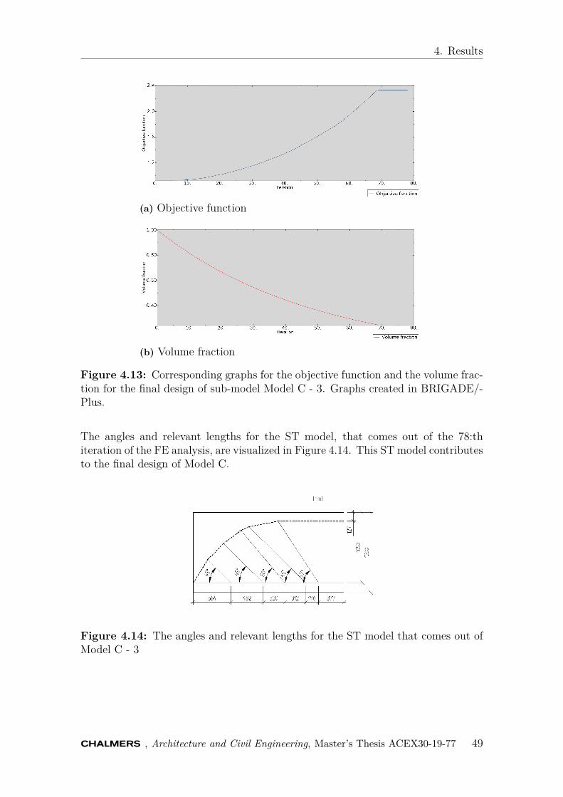
4. Results
(a) Objective function
(b) Volume fraction
Figure 4.13: Corresponding graphs for the objective function and the volume frac-tion for the final design of sub-model Model C - 3. Graphs created in BRIGADE/-Plus.
The angles and relevant lengths for the ST model, that comes out of the 78:thiteration of the FE analysis, are visualized in Figure 4.14. This ST model contributesto the final design of Model C.
Figure 4.14: The angles and relevant lengths for the ST model that comes out ofModel C - 3
, Architecture and Civil Engineering, Master’s Thesis ACEX30-19-77 49

4. Results
4.4 Results from Model CIn this section, the results from Model C are presented, in terms of forces in strutsand ties, checks of critical nodes and the final reinforcement design.
4.4.1 Forces in struts and ties from Model CThe locations and labeling of struts, ties, nodes and external and reaction forces arepresented in Figure 4.15 and the associated magnitudes are presented in Table 4.8.
Figure 4.15: Locations of struts, ties, nodes and external and reaction forces forModel C
Table 4.8: Normal forces in struts and ties together with external and reactionforces for Model C
Strut [kN] Tie [kN] Point loads and reaction force [kN]C1 4 897 T1 787 R1 3 335C2 4 561 T2 633 P1 674C3 4 472 T3 765 P2 485C4 4 560 T4 819 P3 586C5 4 790 T5 1 430 P4 579C6 3 891 T6 4 897 P5 1011
T7 4 492T8 4 085T9 3 594T10 3 015T11 2 004
4.4.2 Check of critical nodes for Model CNode 2 and 11 in Figure 4.15 are the critical nodes in Model C and are checkedagainst the requirements given by Eurocode 2 (2008). The results are presented in
50 , Architecture and Civil Engineering, Master’s Thesis ACEX30-19-77
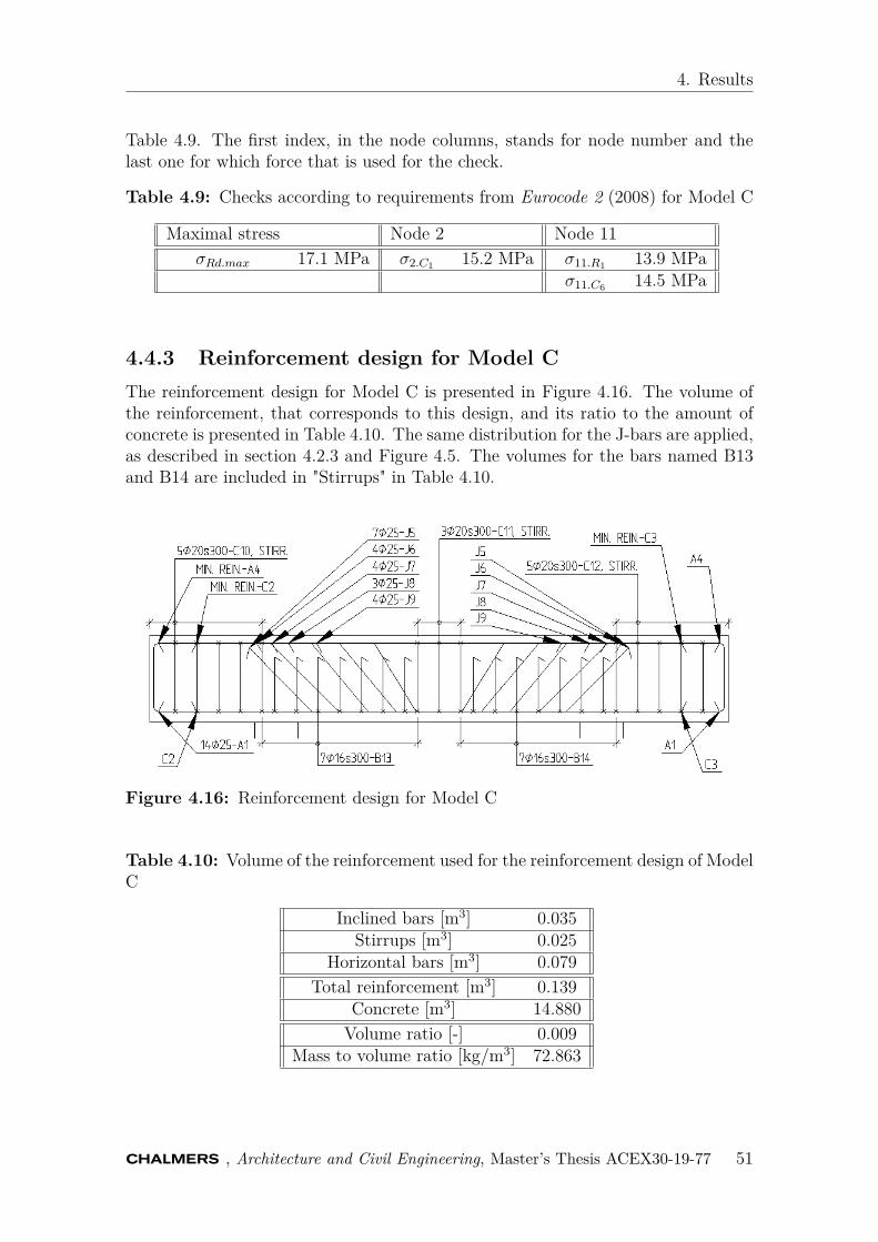
4. Results
Table 4.9. The first index, in the node columns, stands for node number and thelast one for which force that is used for the check.
Table 4.9: Checks according to requirements from Eurocode 2 (2008) for Model C
Maximal stress Node 2 Node 11σRd.max 17.1 MPa σ2.C1 15.2 MPa σ11.R1 13.9 MPa
σ11.C6 14.5 MPa
4.4.3 Reinforcement design for Model CThe reinforcement design for Model C is presented in Figure 4.16. The volume ofthe reinforcement, that corresponds to this design, and its ratio to the amount ofconcrete is presented in Table 4.10. The same distribution for the J-bars are applied,as described in section 4.2.3 and Figure 4.5. The volumes for the bars named B13and B14 are included in "Stirrups" in Table 4.10.
Figure 4.16: Reinforcement design for Model C
Table 4.10: Volume of the reinforcement used for the reinforcement design of ModelC
Inclined bars [m3] 0.035Stirrups [m3] 0.025
Horizontal bars [m3] 0.079Total reinforcement [m3] 0.139
Concrete [m3] 14.880Volume ratio [-] 0.009
Mass to volume ratio [kg/m3] 72.863
, Architecture and Civil Engineering, Master’s Thesis ACEX30-19-77 51

5Discussion
The studies performed in Chapter 2 and 3 together with the results presented inChapter 4 are based on the aim of finding an effective ST model by using struc-tural topology optimization. By adopting the BESO method and applying it on thecrossbeam described in Section 3.1, three types of optimized sub-models could bedeveloped. These sub models were combined into Model C, which was analyzed andthen compared with the models developed by hand, Model A and B. The differentmodels will be discussed in the following sections, including advantages and disad-vantages and problems that arose during this thesis. Finally, the results from thedifferent models will be compared and discussed.
5.1 Model A
Model A was based on the conventional ST method and how IHT implements itwhen designing crossbeams for supports in bridges. The procedure was straightforward and results could be extracted within a day. The method could be used forcrossbeams with different geometries and loading conditions, with few modifications,which made it possible to experiment with the dimensions of the crossbeam. TheST method is a rational approach to how the forces should be modeled and howthe reinforcement should be arranged, which makes it suitable for quick but reliableestimations.
For Model A, the results corresponded well to the documents provided by IHT.However, to get more comparable results to Model B and C, Model A was slightlyoptimized by shortening of the horizontal reinforcement to only fulfill the need fora particular cross-section. In IHT’s reinforcement design, the same amount of hor-izontal reinforcement was placed over the whole crossbeam. This was done sincethe savings from reduction of reinforcement amount was judged to be smaller thanthe cost of adjusting the lengths of the reinforcement bars. Such considerations arecommon in the construction industry, but in this thesis the cost of that somethingis complicated or time consuming to build is not taken into account. Instead, fo-cus was to investigate the reinforcement amount needed and finding an optimal STmodel for this.
Compared to Model B and C, the type of ST modelling applied for Model A, vastlyincreases the need for vertical stirrups, which can be seen in the comparison inTable 5.2. The main reason for this is that the vertical ties carry the load straightvertically while the inclined ties are oriented so that they utilizes the concrete in amore effective way.
52

5. Discussion
5.2 Model BThe procedure of creating Model B was also straightforward and the model could bedeveloped quickly following the procedure presented in Section 3.2.2. Since only fourinclined ties were used, the distance between them became quite large. Therefore, itwas chosen to let the stirrups be placed over the whole beam to satisfy the minimumreinforcement amount.
One question that arose regarding the inclined bars was how complicated and timeconsuming it would be to construct such a reinforcement design and whether or notit is inconvenient for the construction workers. But with the same argument that wasmentioned in previous section, the focus was placed on arranging the reinforcementbars in line with the inclined ties, which resulted in the final designs of this thesis.
5.3 Model CModel C was obtained by using structural topology optimization, namely BESO. Byapplying the BESO algorithm to both 2D and 3D models, optimized models werefound. These models displayed optimums for transferring the distributed load interms of load paths to the supports. Three sub-models were created and similaritiesin load paths were searched for. This allowed the stiffness and load to be treatedarbitrarily, as long as convergence was met. By combining the three sub-models,discussed in the following sections, the final ST model for Model C could be estab-lished. Model C is more complicated than Model A and Model B, and to developand analyze this model has been comparably time consuming.
When comparing the simulations in MATLAB versus BRIGADE/Plus the differencein time, required to run the simulations, should be noted. The required times for thesimulations of Models C - 1, C - 2 and C - 3 are summarized in Table 5.1. As can beseen, the difference in time is huge and therefore MATLAB was an excellent tool forinvestigating the effects of various inputs, which then increased the knowledge for thesimulations in BRIGADE/Plus. The reason to why there is a substantial differencein the computational time, between MATLAB and BRIGADE/Plus, might be thatMATLAB is a computational program which is very efficient when it comes tocreating and compute matrices. Another reason could be how the creation of thefilter map is performed for the different programs, but to draw conclusions regardingthis, more knowledge about the different FEA solvers needs to be obtained.
Table 5.1: Times for simulations of the sub-models
Model Elements Create filter map Performing iterations Total timeC - 1 54 000 3 s 40 s 43 sC - 2 54 000 8 h 20 min 1 h 18 min 9 h 38 minC - 3 128 000 46 h 40 min 2 h 23 min 49 h 3 min
, Architecture and Civil Engineering, Master’s Thesis ACEX30-19-77 53

5. Discussion
5.3.1 Model C - 1This sub-model was created in MATLAB so in this sub-model, many combinationsof inputs could be tested in an time efficient way. This contributed to the un-derstanding of the effects of how the filter radius (rmin) affected the occurrence ofcheckerboard patterns as visualized in Figure 2.11. It also gave insight to how thetwo other parameters, evolutionary ratio (ER) and volume fraction (Vf ), affectedthe results. By using an evolutionary ratio somewhere between 2-4%, the optimizedresults converged while using larger values gave inconsistency in the final models.Vf affected the results of the model in the way that when it got too low, changesin the bottom edge of the crossbeam occurred. For Model C - 1 the consistency ofthe model was kept and an optimized model could be produced even with low Vf .However, for Model C - 2 and Model C - 3, the final result was affected, which willbe discussed in the following subsections.
5.3.2 Model C - 2By varying Vf for the model it could be seen that for Vf < 35% convergence waslost and distortion problem arose. This was due to the fact that elements on thebottom were assigned void properties and therefore the smallest stresses occured inthe nodes of these elements. This is shown in 5.1 where the blue part indicates lowstresses in the elements.
For the optimizations conducted in BRIGADE/Plus it was discovered that the opti-mization simulations became time consuming as the number of elements increased.This problem was reduced by modifications to the python script which allowed tosave the filter map (FM) for models and reuse them for models with the same mesh.Thus, the optimization time could be reduced and optimization simulations couldbe performed during nights and weekends.
5.3.3 Model C - 3Model C - 3 is a 3D model which was translated into a 2D ST model, in order tocombine it with Model C - 1 and Model C - 2. The 3D optimization was performedon a beam modeled with rigid plates as supports. It could be seen from the finalmodel of the beam that two arches were created to transfer the load to the corners ofthe plates. Instead of translating this 3D model into a 2D ST model, the model couldhave been translated into a 3D ST model. With a 3D ST model, the reinforcementcould have a 3D arrangement which might had improved the reinforcement usageeven further.
To reduce the time to create filter maps, it was decided to assign the elementsdifferent lengths in different directions. Since the final objective with the 3D model,in this case, was to find a model that could be translated into a 2D model, theelements were assigned smaller lengths in x- and y-direction than in z-direction.This was made since the beam was simply supported meaning that the load wascarried mainly in the xy-plane and not in the z-direction.
54 , Architecture and Civil Engineering, Master’s Thesis ACEX30-19-77

5. Discussion
(a) Iteration 56 undistorted
(b) Iteration 57 distorted
Figure 5.1: Iteration step 56 and 57 displaying how the code assigns void propertiesto the elements on the bottom edge which leads to distortion in iteration step 57
5.3.4 Convergence of the sub-modelsA big part of the model development was understanding how the optimization rou-tine worked and what inputs and refinements to the models were needed to getconverging results.
One major issue to overcome in this thesis was to deal with the distortion of elementsused in the simulations. A trial and error process was conducted to overcome theobstacle of elements distortion which affected the final results of the BESO iterations.By plotting the objective function and the volume fraction, as visualized in e.g.Figure 4.13, a tool for convergence investigation was obtained. The two curvesshould correlate to each other in order to obtain good results. It could be seenthat if the objective function had "spikes" that disrupted the graph as visualized inFigure 5.2, distortion of elements had occurred. The graph in Figure 5.2 describesthe objective function for the analysis shown in Figure 5.1. Distortion can indicateexcessive increase in external work, but since the load was constant on the structure
, Architecture and Civil Engineering, Master’s Thesis ACEX30-19-77 55

5. Discussion
the spikes here implicated that the elemental strains increased towards infinity as aresult of element distortions.
Figure 5.2: Objective function with distorting elements
One reason why this happened could be that the filter scheme, applied in the pythoncode, was too rough and would need further improvement. Another reason couldbe that the mesh was to coarse or that an element type that is too sensitive todistortion was used. It was also discovered that when the BESO algorithm switchestwo elements that shared the same node into void elements, and the same elementswere subjected to external load in the next iteration, distortion was unavoidable.
Distortion was not a problem for Model C - 1 so improvements were only done forModel C - 2 and Model C - 3. For Model C - 2 it was discovered that a Vf = 35%together with second order elements with reduced integration (CPS8R) gave resultsresembling the results obtained by Model C - 1. For Model C - 3 the problem wassolved by applying a load dividing thin shell on the bottom of the beam, used todistribute the load, and by applying 8 node brick elements and reduced integrationwith enhanced hourglass control (C3D8R).
Even though the spikes on the objective function curve indicate problem with themodels, there was a possibility that the results could be useful anyway. If the results,i.e. the model to be translated into a ST-model, was extracted from iterations beforeor after the element distortion, reasonable models could be obtained in many cases.
Another thing that affected the final results was to choose the right rmin. Fromliterature it was found that a sufficient rmin should be around three times the elementsize. To confirm this, optimization was performed on the same model but withalternating rmin. For Model C - 2 and Model C - 3, a rmin of approximately threetimes the largest element length was found suitable, while for Model C - 1 an rminof six times the element length gave similar results as the other models.
5.4 Comparison between the modelsThe comparison of the reinforcement volume for the final design is presented inTable 5.2. Following notes can be made regarding the results shown in this table.
56 , Architecture and Civil Engineering, Master’s Thesis ACEX30-19-77

5. Discussion
The difference in horizontal reinforcement bars is relatively small. This means thatall models have similar need for horizontal reinforcement in the bottom part of thebeam, which is reasonable since geometry and loading conditions are the same. ForModel B and C, there is more reinforcement bars placed in mid span than what themiddle tie requires. The reason for this is that the J-bars deviates at certain sectionswhile the requirement for the ties closest to support still needs to be satisfied. Thismeans that it might be possible to further optimize the models by e.g. using otherangles for the ties.
The need for stirrups is the largest factor to the difference in the final results. ModelA uses vertical stirrups to take care of the lifting of the forces, while this is takencare of by the inclined ties in Model B and C. Even though the ULS requirementis met by all ST models, the requirement of maximum center to center distancebetween reinforcement bars has to be fulfilled. Therefore, Model B and C has beenassigned the largest allowable center to center distance of 300 mm for the stirrups,which corresponds to the maximum distance chosen for this thesis. This means thatthe vertical stirrups in mid span in Model B and C do not fulfill any particularpurpose when it comes to lifting of the forces, which in turn means that the span isoversized for those two models.
Table 5.2: Comparison of the reinforcement volume for the final designs
Model Inclined bars [m3] Stirrups [m3] Horizontal bars [m3] Sum [m3]A - 0.087 0.085 0.172B 0.047 0.039 0.083 0.169C 0.035 0.025 0.079 0.139
In Table 5.3, the forces in the ties are summarized. All the tie forces that are nothorizontal are summarized in "Sum of the lifting ties" while the largest single tieforce in the mid span is presented in "Horizontal tie in mid span". Thus, there aresome horizontal tie forces that are excluded in this table, since they are not relevantfor this discussion.
It is clear that the forces in the lifting ties become larger as the the angle betweenthe horizontal ties and the lifting ties increases. This is reasonable using simpletrigonometry knowledge, but it also means that the forces in the compression strutsbecome larger. Therefore, a ST model with inclined ties utilizes the compressionstrength of the concrete in a more efficient way. Another note to make, regardingthis phenomena, is that the force in the horizontal tie in mid span becomes largeras the forces in the lifting ties decrease. This is also logical since the inclined tiescontribute with horizontal tension in the bottom layer.
For this type of structural element, it is common to place an amount of horizontalreinforcement bars that satisfy the requirement given by the mid span tie along thewhole crossbeam. As mentioned in Section 5.1, this simplification is not done inthis thesis since the optimal design is sought for. It is clear, if comparing Table
, Architecture and Civil Engineering, Master’s Thesis ACEX30-19-77 57

5. Discussion
5.2 to Table 5.3, that even though the tie force is the smallest for Model A, thereinforcement design for Model A uses the largest horizontal reinforcement amount.The reason for this is, as mentioned in Section 5.1, that shortening of the horizontalreinforcement bars is taken into account. The need in mid span is the largest forModel C, but this need is also required along a shorter length.
Table 5.3: Comparison of forces in the ties
Model Sum of the lifting ties [kN ] The horizontal tie in mid span [kN ]A 6 543 4 022B 5 436 4 752C 4 434 4 897
58 , Architecture and Civil Engineering, Master’s Thesis ACEX30-19-77

6Conclusion
The aim of this master thesis was to investigate the potential in using structuraloptimization to find effective ST models. This has been achieved by performing acase study on a crossbeam designed by the civil engineering company Inhouse TechAB. By applying structural optimization, in this thesis BESO, to both 2D and 3Dmodels it was shown that it is possible to use structural optimization to generateeffective ST models, which also proves the statement about conventional ST methodbeing over-conservative.
Regarding the convergence of the models, it could be seen that the inputs and howthe model was constructed had a large influence of how the final results came out.The filter radius, volume fraction and type of element needed to be chosen correctly.It was found that to get coherent models, the filter radius for Model C - 1 should bearound six times the element size, while for Model C - 2 and C - 3, it was sufficientwith three times the largest element size. The volume fraction was chosen to 45%,35% and 25% for the three sub-models.
It can also be concluded that the development of the objective function is an im-portant indicator for how the final model is going to look. The development of theobjective function needs to reflect the development of the volume fraction curve.Otherwise it was proven that, in most cases, convergence was lost and the resultscould not be translated to a ST model.
By comparing Model A, Model B and Model C it can be seen that the influence ofinclined reinforcement contributes to a more efficient utilization of the compressivestrength of the concrete, which leads to a reduced need of reinforcement. For thecase study in this thesis, it was seen that when comparing Model B and C to ModelA, the reduction of reinforcement is 1.7% and 19.2%, respectively.
By studying Shobeiri & Ahmadi-Nedushan (2017) it could be seen that BESO wasapplicable to a wide range of different types of structural problems. This means thatthis method of finding an effective ST model can be applied to structural elementswere the load paths is hard to predict in an analytical way.
BRIGADE/Plus, together with the Python script used, were not optimal for struc-tural optimization. It was time consuming to build appropriate models and the finalresults were much dependent on the different inputs. In addition, the simulationsrequired much time. The m-script was much more time efficient to use. In this scriptthe model was already built within the script and this saved a lot of time. However,the m-script was limited to only perform 2D analysis and to perform structural op-
59

6. Conclusion
timization on a beam with three different load cases and boundary conditions. Tobuild different models in MATLAB would of course be possible to do but this, onthe other hand, is much more convinient to do in BRIGADE/Plus.
60 , Architecture and Civil Engineering, Master’s Thesis ACEX30-19-77

7Further work
The optimization routine could easily be extended to investigate other commonlyused ST-models in order to refine how they are structured in accordance to Eurocode.
As mentioned in section 3.1 the load is assumed to act at the bottom of the cross-beam, but in the real case it is distributed over the height of the beam. By modelingthe whole system, crossbeams and main girder, with the correct loads applied, BESOcould be used to find and investigate the load paths from the main girder via thecrossbeam to the supports. In this way, conclusions regarding how the load couldbe applied to the ST models developed in this thesis, could be drawn. This couldcontribute to refinement of the ST models used when designing crossbeams.
Since this thesis has dealt with the development of ST models, which are valid forULS only, SLS calculations also needs to be performed. This, in combination withthe question of whether the handling of inclined ties are too complex or not, wouldbe a suiting continuation for further work.
As mentioned in conclusion, the software used in this thesis were not optimal forstructural optimization. Another further work could be to use commercial optimiza-tion software, such as TOSCA, and develop a routine for designing 3D ST models.Since commercial software are more refined than the Python script used in this the-sis, reduced computational times and less complications with the models could beexpected. Thus, by developing a routine that could be applied to a wide range ofdifferent structures, it would be possible to help the designer in her/his everydaywork.
61

References
Austrell, P.-E., Dahlbom, O., Lindeman, J., Olsson, A., Olsson, K.-G., Persson, K.,Petersson, H., Ristinmaa, M., Sandberg, G. & Wernberg, P.-A. (2004), CALFEM,A FINITE ELEMENT TOOLBOX, version 3.4 edn, Lund.
BRIGADE/Plus 6.2-5 (2019).URL: https://scanscot.com/products/bridge-design/brigade-plus/
Christiansen, P. W. & Klarbring, A. (2009), An Introduction to Structural Opti-mization, Springer, Linköping.
Dahl, T. (2018), Optimering av böjarmering genom FEM-analys och strut-and-tiemodellering, Technical report, Division of Structural Mechanics, LTH, Lund.
Defining rigid body constraints (2017).URL: https://abaqus-docs.mit.edu/2017/English/SIMACAECAERefMap/simacae-t-itnhelptopicrigid.htm
Engström, B. (2011), Design and analysis of deep beams, plates and other disconti-nuity regions., Chalmers University of Technology, Göteborg.
Eurocode 2 (2008), ss-en 1992-1-1:2005 edn, SIS, Stockholm.
Hendy C. R. & Smith D. A. (2007), Designers’ Guide to En 1992-2. Eurocode 2:Design of Concrete Structures. Part 2: Concrete Bridges, ICE Publishing, Lon-don.
Huang, X. X. & Xie, Y. M. (2010), Evolutionary topology optimization of continuumstructures : methods and applications, Wiley.
Mathern, A. & Chantelot, G. (2010), Strut-and-tie modelling of reinforced concretepile caps, Technical report, Division of Structural Engineering, Gothenburg.
Mathern, A., Chantelot, G., Svahn, P.-O., Kettil, P., Rasmus, R. & Engström, B.(2017), Enhanced strut-and-tie model for reinforced concrete pile caps, Technicalreport, IABSE Symposium, Vancouver.
Obbink-Huizer, C. (2018), ‘Automate boring postprocessing in Abaqus using pythonscripting’.URL: https://info.simuleon.com/blog/automate-boring-postprocessing-in-abaqus-using-python-scripting
Osvaldo M, Q., Mariano, V., Cristina, A., Rubén, A. & Pascual, M. (2017), TopologyDesign Methods for Structural Optimizaation, Elsevier Ltd, London.
62

References
Plevris, V. & Tsiatas, G. C. (2018), ‘Computational Structural Engineering: PastAchievements and Future Challenges’, Frontiers in Built Environment 4.
Python Software Foundation (2019), ‘11.1. pickle — Python object serialization —Python 2.7.16 documentation’.URL: https://docs.python.org/2/library/pickle.html
Qing Quan Liang, Xie, Y. M. & Grant Prentice Steven (2000), ‘Topology Opti-mization of Strut-and-Tie Models in Reinforced Concrete Structures Using anEvolutionary Procedure’, ACI Structural Journal (2).
Saabye Ottosen, N. & Petersson, H. (1992), Introduction to the finite elementmethod, Prentice Hall, New York.
Saraswat, S. (n.d.), ‘Python Language Introduction - GeeksforGeeks’.
Shobeiri, V. & Ahmadi-Nedushan, B. (2017), ‘Bi-directional evolutionary structuraloptimization for strut-and-tie modelling of three-dimensional structural concrete’,Engineering Optimization .
Vishark, R. (n.d.), ‘What are the three main criteria to determine the slave andmaster surfaces in ABAQUS? - Quora’.
Xia, L., Xia, Q., Huang, X. & Xie, Y. M. (2016), ‘Bi-directional Evolutionary Struc-tural Optimization on Advanced Structures and Materials: A Comprehensive Re-view’, Archives of Computational Methods in Engineering .
Zuo, Z. H. & Xie, Y. M. (2015), ‘A simple and compact Python code for complex3D topology optimization’, Advances in Engineering Software .
, Architecture and Civil Engineering, Master’s Thesis ACEX30-19-77 63

AHand calculations
A.1 Hand calculations on Model A
I

Angles
≔y =atan⎛⎜⎝――
-d e
D
⎞⎟⎠
58.419
≔x =-90 y 31.581
≔w =atan⎛⎜⎝――
-d e
C
⎞⎟⎠
58.419
≔v =-90 w 31.581
≔s =atan⎛⎜⎝――
-d e
B
⎞⎟⎠
58.419
≔u =-90 s 31.581
Loads
≔Vd 1779
≔PEd 6670
≔R1 =――PEd
23335
≔qEd =――PEd
L1.482 ――
≔P1 =⋅qEd⎛⎜⎝
+A ―B
2
⎞⎟⎠
1170.956
≔P2 =⋅qEd⎛⎜⎝
+―B
2―C
2
⎞⎟⎠
865.618
≔P3 =⋅qEd⎛⎜⎝
+―C
2D
⎞⎟⎠
1298.427
≔P =++P1 P2 P3 3335 =R1 3335 OK

Forces in the truss
≔T1 =P1 1170.956
≔C1 =―――T1
cos ((u))1374.515
≔T2 =+P2 ⋅C1 cos ((u)) 2036.573
≔C2 =―――T2
cos ((v))2390.612
≔T3 =+P3 ⋅C2 cos ((v)) 3335
≔C3 =―――T3
cos ((x))3914.758 ≔R1 =⋅C3 sin((y)) 3335 OK
≔C6 =⋅C3 sin((x)) 2050.147
≔C5 =+C6 ⋅C2 sin((v)) 3302.104
≔C4 =+C5 ⋅C1 sin((u)) 4021.934
≔T7 =⋅C3 cos ((y)) 2050.147
≔T6 =+T7 ⋅C2 cos ((w)) 3302.104
≔T5 =+T6 ⋅C1 cos ((s)) 4021.934
≔T4 =T5 4021.934 =C4 4021.934 OK

Check of nodes
Compression - tension node with anchored ties in one direction and where the the bars are
anchored within the node.
≔fck 35
≔fcd =――fck
1.523.333
≔k2 0.85
≔ν =-1 ――――fck
2500.86
≔σrd.max =⋅⋅k2 ν fcd 17.057
Control of node 7
≔u =⋅2 (( -H d)) 300
≔a1 400
≔b1 600
≔a2 =+⋅a1 sin ((y)) ⋅u cos ((y)) 497.871
≔b2 =b1 600
≔σd1.7 =――R1
⋅a1 b113.896 OK
≔σd2.7 =――C3
⋅a2 b213.105 OK

Control of node 2
≔a1 =⋅2 e 200
≔b1 =b 1550
≔σd1.2 =――C4
⋅a1 b112.974 OK
Design of ties
≔fst 300 ≔fyk 500
≔fst.lift 435
Vertical reinforcement:
Reinforcement equal to T1 is used on the length =+A ―B
2790
≔AsT1 =――T1
fst.lift2691.852 2 ≔AsiT1 314 2 d=20mm
≔nT1 =――AsT1
AsiT1
8.573 ≔nT1 9 Number of stirrups
Reinforcement equal to T2 is used on the length =+―B
2―C
2584
≔AsT2 =――T2
fst.lift4681.778 2 ≔AsiT2 314 2
≔nT2 =――AsT2
AsiT2
14.91 ≔nT2 15
Reinforcement equal to T3 is used on the length =+―C
2D 876
≔AsT3 =――T3
fst.lift7666.667 2 ≔AsiT3 314 2
≔nT3 =――AsT3
AsiT3
24.416 ≔nT3 25

Total amount of lifting reinforcement:
≔Alift =++⋅2 AsT1 ⋅2 AsT2 ⋅2 AsT3 30080.593 2
Horizontal reinforcement
≔AsT4 =―T4
fst13406.445 2 ≔AsiT4 491 2 d=25mm
≔nT4 =――AsT4
AsiT4
27.304 ≔nT3 28
Total amount of reinforcement:
=Alift 30080.593 2
≔Ahorizontal =AsT4 13406.445 2
≔Atot =+Alift Ahorizontal 43487.038 2
Reinforcement design
Bars
≔ϕhorisontal 25
≔As.i.h =―――――⋅ϕhorisontal
2
4490.874 2
≔ϕvertical 20
≔As.i.v =――――⋅ϕvertical
2
4314.159 2
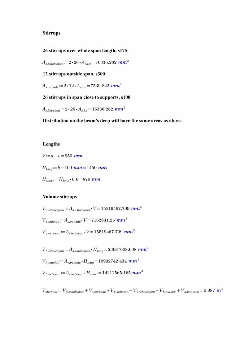
Stirrups
26 stirrups over whole span length, s175
≔As.wholespan =⋅⋅2 26 As.i.v 16336.282 2
12 stirrups outside span, s300
≔As.outside =⋅⋅2 12 As.i.v 7539.822 2
26 stirrups in span close to supports, s100
≔As.between =⋅⋅2 26 As.i.v 16336.282 2
Distribution on the beam's deep will have the same areas as above
Lengths
≔V =-d e 950
≔Hlong =-b 100 1450
≔Hshort =⋅Hlong 0.6 870
Volume stirrups
≔Vv.wholespan =⋅As.wholespan V 15519467.709 3
≔Vv.outside =⋅As.outside V 7162831.25 3
≔Vv.between =⋅As.between V 15519467.709 3
≔Vh.wholespan =⋅As.wholespan Hlong 23687608.608 3
≔Vh.outside =⋅As.outside Hlong 10932742.434 3
≔Vh.between =⋅As.between Hshort 14212565.165 3
≔Vstirr.tot =+++++Vv.wholespan Vv.outside Vv.between Vh.wholespan Vh.outside Vh.between 0.087 3

Horizontal reinforcement
Distance AB ≔ABh 3764
Distance C ≔Ch 4932
Distance D ≔Dh 7900
Need on lenth A:
≔As.T4 =―T4
fst13406.445 2
≔nT4 =――As.T4
As.i.h
27.311 ≔nT4 =ceil ⎛⎝nT4⎞⎠ 28
≔As.T4.real =⋅nT4 As.i.h 13744.468 2
Need on lenth B:
≔As.T5 =―T5
fst13406.445 2
≔nT5 =――As.T5
As.i.h
27.311 ≔nT5 =ceil ⎛⎝nT5⎞⎠ 28
≔As.T5.real =⋅nT5 As.i.h 13744.468 2
Need on lenth C:
≔As.T6 =―T6
fst11007.013 2
≔nT6 =――As.T6
As.i.h
22.423 ≔nT6 =ceil ⎛⎝nT6⎞⎠ 23
≔As.T6.real =⋅nT6 As.i.h 11290.099 2

Need on lenth D:
≔As.T7 =―T7
fst6833.825 2
≔nT7 =――As.T7
As.i.h
13.922 ≔nT7 =ceil ⎛⎝nT7⎞⎠ 14
≔As.T7.real =⋅nT7 As.i.h 6872.234 2
Volume of horisontal reinforcement
≔VD =⋅⋅As.i.h nT7 Dh 54290648.045 3
≔VC =⋅⋅As.i.h⎛⎝ -nT6 nT7
⎞⎠ Ch 21788908.548 3
≔VAB =⋅⋅As.i.h⎛⎝ -nT5 nT6
⎞⎠ ABh 9238245.897 3
≔Vh.tot =++VD VC VAB 0.085 3
Total volume of reinforcement
≔Vtot.rein =+Vh.tot Vstirr.tot 0.172 3

A. Hand calculations
A.2 Hand calculations on Model B
X , Architecture and Civil Engineering, Master’s Thesis ACEX30-19-77

Angles
≔θ1 75≔θ2 =θ1 75
≔α1 35
≔α2 55≔α3 31≔α4 59
Loads
≔PEd 6670
≔R1 =――PEd
23335
≔qEd =――PEd
L1.482 ――
≔P1 =⋅qEd
⎛⎜⎝
+A ―B
2
⎞⎟⎠
1915.772
≔P2 =⋅qEd
⎛⎜⎝
+―B
2C
⎞⎟⎠
1419.228
≔P =+P1 P2 3335 OK
Forces in the truss
Node 5
≔C2 =―――R1
sin⎛⎝α4⎞⎠
3890.722
≔T5 =⋅C2 cos ⎛⎝α4⎞⎠ 2003.87

Node 4
≔T2 =――――⋅C2 cos ⎛⎝α3
⎞⎠
sin⎛⎝θ2⎞⎠
3452.646
≔C4 =+⋅T2 cos ⎛⎝θ2⎞⎠ ⋅C2 sin⎛⎝α3
⎞⎠ 2897.481
Node 3
≔C1 =―――――-⋅T2 sin⎛⎝θ2
⎞⎠ P2
sin ⎛⎝α2⎞⎠
2338.726
≔T4 =++⋅C1 cos ⎛⎝α2⎞⎠ ⋅T2 cos ⎛⎝θ2
⎞⎠ T5 4238.919
Node 2
≔T1 =――――⋅C1 cos ⎛⎝α1
⎞⎠
sin⎛⎝θ1⎞⎠
1983.353
≔C3 =++C4 ⋅C1 sin⎛⎝α1⎞⎠ ⋅T1 cos ⎛⎝θ1
⎞⎠ 4752.248
Node 1
≔T3 =+⋅T1 cos ⎛⎝θ1⎞⎠ T4 4752.248 =C3 4752.248 OK

Check of nodes
Compression - tension node with anchored ties in one direction and where the the bars are
anchored within the node.
≔fck 35
≔fcd =――fck
1.523.333
≔k2 0.85
≔ν =-1 ――――fck
2500.86
≔σrd.max =⋅⋅k2 ν fcd 17.057
Control of node 5
≔u =⋅2 (( -H d)) 300
≔a1 400
≔b1 600
≔a2 =+⋅a1 sin ⎛⎝α4⎞⎠ ⋅u cos ⎛⎝α4
⎞⎠ 497.378
≔b2 =b1 600
≔σd1.5 =――R1
⋅a1 b1
13.896 OK
≔σd2.5 =――C2
⋅a2 b2
13.037 OK

Control of node 2
≔a1 =⋅2 e 200
≔b1 =b 1550
≔σd1.2 =――C3
⋅a1 b1
15.33 OK
Design of ties
≔fst 300
≔fst.lift 435
Reinforcement equal to T1 is used on the length =+A ―B
21292.5
With an angle of 75 deg
≔AsT1 =――T1
fst.lift4559.433 2 ≔AsiT1 201 2 d=20mm
≔nT1 =――AsT1
AsiT1
22.684 ≔nT1 23
Reinforcement equal to T2 is used on the length =+―B
2C 957.5
With an angle of 75 deg
≔AsT2 =――T2
fst.lift7937.117 2 ≔AsiT2 201 2 d=20mm
≔nT2 =――AsT2
AsiT2
39.488 ≔nT2 40

Total amount of lifting reinforcement:
≔Alift =+⋅2 AsT1 ⋅2 AsT2 24993.101 2
Horizontal reinforcement
≔AsT3 =―T3
fst15840.828 2 ≔AsiT3 314 2
d=25mm
≔nT3 =――AsT3
AsiT3
50.448 ≔nT3 49
Total amount of reinforcement:
=Alift 24993.101 2
≔Ahorizontal =AsT3 15840.828 2
≔Atot =+Alift Ahorizontal 40833.929 2

Reinforcement design
Bars
≔ϕ 25
≔As.i.h =――⋅ϕ2
4490.874 2
≔ϕvertical 20
≔As.i.v =――――⋅ϕvertical
2
4314.159 2
Distances
≔Arein 996
≔Brein 2834
≔Crein 7900
Need on distance tie T3
≔As.T3 =―T3
fst15840.828 2
≔nT3 =――As.T3
As.i.h
32.271 ≔nT3 =ceil ⎛⎝nT3⎞⎠ 33 Need
≔nT3 41 To satisfy need in T5
Need for the inclined tie T1
≔As.T1 =――T1
fst.lift4559.433 2
≔nT1 =――As.T1
As.i.h
9.288 ≔nT1 =ceil ⎛⎝nT1⎞⎠ 10

Need on distance tie T4
≔As.T4 =―T4
fst14129.73 2
≔nT4 =――As.T4
As.i.h
28.785 ≔nT4 =ceil ⎛⎝nT4⎞⎠ 29 Need
≔nT4 =-nT3 nT1 31 To satisfy need in T5
Need for the inclined tie T2
≔As.T2 =――T2
fst.lift7937.117 2
≔nT2 =――As.T2
As.i.h
16.169 ≔nT2 =ceil ⎛⎝nT2⎞⎠ 17
Need on distance tie T5
≔As.T5 =―T5
fst6679.567 2
≔nT5 =――As.T5
As.i.h
13.608 ≔nT5 =ceil ⎛⎝nT5⎞⎠ 14 Need
≔nT5 =-nT4 nT2 14 To satisfy need in T5
Volume
Bottom layer
Distance C
≔Vh.C =⋅⋅nT5 As.i.h Crein 54290648.045 3
Distance B
≔Vh.B =⋅⋅⎛⎝nT2⎞⎠ As.i.h Brein 23649320.448 3
Distance A
≔Vh.A =⋅⋅nT1 As.i.h Arein 4889103.567 3
Total horizaontal reinforcement
≔Vh.tot =++Vh.A Vh.B Vh.C 0.083 3
Inclined reinforcement
Distances inclined ties plus förankringslängd
≔dT =+985 800 1.785
Volumes
≔Vi.T1 =⋅⋅As.i.h nT1 dT 8762098.26 3
≔Vi.T2 =⋅⋅As.i.h nT2 dT 14895567.043 3
≔Vi.tot =⋅2 ⎛⎝ +Vi.T1 Vi.T2⎞⎠ 0.047 3 Both sides (*2)
Stirrups for minimum reinforcement
≔nstirr 26
≔hstirr =-d e 950
≔bstirr =-b 100 1450
≔As.stirr =⋅nstirr As.i.v 8168.141 2
≔Vstirr =⋅As.stirr⎛⎝ +⋅2 hstirr ⋅2 bstirr
⎞⎠ 0.039 3
Total reinforcement
≔Vrein.tot =++Vstirr Vi.tot Vh.tot 0.169 3

A. Hand calculations
A.3 Hand calculations on Model C
, Architecture and Civil Engineering, Master’s Thesis ACEX30-19-77 XIX

Angles
≔θ1 59 ≔α21 59 ≔α41 10 ≔α61 24≔θ2 50 ≔α22 31 ≔α42 50 ≔α62 50≔θ3 50 ≔α23 80 ≔α43 40 ≔α63 40≔θ4 45 ≔α44 66 ≔α64 52≔θ5 45
≔α81 38 ≔α101 51 ≔α111 59≔α82 45 ≔α102 45≔α83 45 ≔α103 45≔α84 39 ≔α104 31
Loads
≔PEd 6670
≔qEd =――PEd
L1482.222 ―― ≔R1 =――
PEd
23335
≔P1 =⋅qEd
⎛⎜⎝
+A ―B
2
⎞⎟⎠
674.411
≔P2 =⋅qEd
⎛⎜⎝
+―B
2―C
2
⎞⎟⎠
484.687
≔P3 =⋅qEd
⎛⎜⎝
+―C
2―D
2
⎞⎟⎠
586.219
≔P4 =⋅qEd
⎛⎜⎝
+―D
2―E
2
⎞⎟⎠
578.808
≔P5 =⋅qEd
⎛⎜⎝
+―E
2F
⎞⎟⎠
1010.876
≔P =++++P1 P2 P3 P4 P5 3335 OK
Forces in the truss
≔T1 =―――P1
sin⎛⎝θ1⎞⎠
786.791
≔T2 =―――P2
sin⎛⎝θ2⎞⎠
632.714
≔T3 =―――P3
sin⎛⎝θ3⎞⎠
765.254
≔T4 =―――P4
sin⎛⎝θ4⎞⎠
818.558
≔T5 =―――P5
sin⎛⎝θ5⎞⎠
1429.594
≔Ttot =++++T1 T2 T3 T4 T5 4432.91
Starting from node 11, using x-components in every node except node 11
Node 11:
≔C6 =―――R1
sin⎛⎝α111⎞⎠
3890.722
≔T11 =⋅C6 cos ⎛⎝α111⎞⎠ 2003.87
Node 10:
≔C5 =―――――――――+⋅C6 cos ⎛⎝α111
⎞⎠ ⋅T5 cos ⎛⎝α102⎞⎠
cos ⎛⎝α101⎞⎠
4790.478
Node 8:
≔C4 =―――――――――+⋅C5 sin⎛⎝α84
⎞⎠ ⋅T4 cos⎛⎝α82⎞⎠
cos ⎛⎝α81⎞⎠
4560.285
Node 6:
≔C3 =―――――――――+⋅C4 sin⎛⎝α64
⎞⎠ ⋅T3 cos⎛⎝α62⎞⎠
cos ⎛⎝α61⎞⎠
4472.081

Node 4:
≔C2 =―――――――――+⋅C3 sin⎛⎝α44
⎞⎠ ⋅T2 cos⎛⎝α42⎞⎠
cos ⎛⎝α41⎞⎠
4561.449
Node 2:
≔C1 =+⋅C2 sin⎛⎝α23⎞⎠ ⋅T1 cos⎛⎝α21
⎞⎠ 4897.377
Node 9:
≔T10 =+T11 ⋅T5 cos ⎛⎝θ5⎞⎠ 3014.746
Node 7:
≔T9 =+T10 ⋅T4 cos ⎛⎝θ4⎞⎠ 3593.553
Node 5:
≔T8 =+T9 ⋅T3 cos ⎛⎝θ3⎞⎠ 4085.45
Node 3:
≔T7 =+T8 ⋅T2 cos ⎛⎝θ2⎞⎠ 4492.15
Node 1: Compare:
≔T6 =+T7 ⋅T1 cos ⎛⎝θ1⎞⎠ 4897.377 =C1 4897.377 OK
Lifting reinforcement:
≔Tlift =++++T1 T2 T3 T4 T5 4432.91

Check of nodes
≔fck 35
≔fcd =――fck
1.523.333
≔k2 0.85
≔ν =-1 ――――fck
2500.86
≔σrd.max =⋅⋅k2 ν fcd 17.057
Control of node 11
≔u =⋅2 (( -H d)) 300
≔a1 600
≔b1 400
≔a2 =+⋅a1 sin ⎛⎝α111⎞⎠ ⋅u cos ⎛⎝α111
⎞⎠ 0.669
≔b2 =b1 0.4
≔σd1.9 =――R1
⋅a1 b113.896
≔σd2.9 =――C6
⋅a2 b214.543
Both controls OK

Control of node 2
≔a1 =⋅2 e 208
≔b1 =b 1550
≔σd1.2 =――C1
⋅a1 b115.19
OK
Design of ties
≔fst 300
≔fst.lift 435
Inclined reinforcement:
Reinforcement equal to T1 is used on the length =+A ―B
2455
With an angle of 59 deg
≔AsT1 =――T1
fst.lift1808.714 2 ≔AsiT1 314 2 d=20mm
≔nT1 =――AsT1
AsiT1
5.76 ≔nT1 6 Number of stirrups
Reinforcement equal to T2 is used on the length =+―B
2―C
2327
With an angle of 50 deg
≔AsT2 =――T2
fst.lift1454.514 2 ≔AsiT2 314 2
≔nT2 =――AsT2
AsiT2
4.632 ≔nT2 5

Reinforcement equal to T3 is used on the length =+―C
2―D
2395.5
With an angle of 50 deg
≔AsT3 =――T3
fst.lift1759.206 2 ≔AsiT3 314 2
≔nT3 =――AsT3
AsiT3
5.603 ≔nT3 6
Reinforcement equal to T4 is used on the length =+―D
2―E
2390.5
With an angle of 45 deg
≔AsT4 =――T4
fst.lift1881.742 2 ≔AsiT4 314 2
≔nT4 =――AsT4
AsiT4
5.993 ≔nT4 6
Reinforcement equal to T5 is used on the length =+―E
2F 682
With an angle of 45 deg
≔AsT5 =――T5
fst.lift3286.423 2 ≔AsiT5 314 2
≔nT5 =――AsT5
AsiT5
10.466 ≔nT4 11
Total amount of lifting reinforcement:
≔Alift =++++⋅2 AsT1 ⋅2 AsT2 ⋅2 AsT3 ⋅2 AsT4 ⋅2 AsT5 20381.196 2

Horizontal reinforcement
≔AsT6 =―T6
fst16324.59 2 ≔AsiT6 491 2 d=25mm
≔nT5 =――AsT6
AsiT6
33.248 ≔nT6 34
Total amount of reinforcement
=Alift 20381.196 2
≔Ahorizontal =AsT6 16324.59 2
≔Atot =+Alift Ahorizontal 36705.786 2
Reinforcement design
Bars
≔ϕ 25
≔As.i.h =――⋅ϕ2
4490.874 2
≔ϕvertical 20
≔As.i.v =――――⋅ϕvertical
2
4314.159 2
≔ϕbmin 16
≔As.i.bmin =――――⋅ϕbmin
2
4201.062 2

Distances
≔Arein 641 ≔Drein 2759
≔Brein 1177 ≔Erein 3512
≔Crein 1950 ≔Frein 7900
Need on distance tie T6
≔As.T6 =―T6
fst16324.59 2
≔nT6 =――As.T6
As.i.h
33.256 ≔nT6 =ceil ⎛⎝nT6⎞⎠ 34 Need
≔nT6 36 To satisfy need in T11
Need for the inclined tie T1
≔As.T1 =――T1
fst.lift1808.714 2
≔nT1 =――As.T1
As.i.h
3.685 ≔nT1 =ceil ⎛⎝nT1⎞⎠ 4
Need on distance tie T7
≔As.T7 =―T7
fst14973.833 2
≔nT7 =――As.T7
As.i.h
30.504 ≔nT7 =ceil ⎛⎝nT7⎞⎠ 31 Need
≔nT7 =-nT6 nT1 32 To satisfy need in T11

Need for the inclined tie T2
≔As.T2 =――T2
fst.lift1454.514 2
≔nT2 =――As.T2
As.i.h
2.963 ≔nT2 =ceil ⎛⎝nT2⎞⎠ 3
Need on distance tie T8
≔As.T8 =―T8
fst13618.165 2
≔nT8 =――As.T8
As.i.h
27.743 ≔nT8 =ceil ⎛⎝nT8⎞⎠ 28 Need
≔nT8 =-nT7 nT2 29 To satisfy need in T11
Need for the inclined tie T3
≔As.T3 =――T3
fst.lift1759.206 2
≔nT3 =――As.T3
As.i.h
3.584 ≔nT3 =ceil ⎛⎝nT3⎞⎠ 4
Need on distance tie T9
≔As.T9 =―T9
fst11978.512 2
≔nT9 =――As.T9
As.i.h
24.402 ≔nT9 =ceil ⎛⎝nT9⎞⎠ 25 Need
≔nT9 =-nT8 nT3 25 To satisfy need in T11

Need for the inclined tie T4
≔As.T4 =――T4
fst.lift1881.742 2
≔nT4 =――As.T4
As.i.h
3.833 ≔nT4 =ceil ⎛⎝nT4⎞⎠ 4
Need on distance tie T10
≔As.T10 =――T10
fst10049.152 2
≔nT10 =――As.T10
As.i.h
20.472 ≔nT10 =ceil ⎛⎝nT10⎞⎠ 21 Need
≔nT10 =-nT9 nT4 21 To satisfy need in T11
Need for the inclined tie T5
≔As.T5 =――T5
fst.lift3286.423 2
≔nT5 =――As.T5
As.i.h
6.695 ≔nT5 =ceil ⎛⎝nT5⎞⎠ 7
Need on distance tie T11
≔As.T11 =――T11
fst6679.567 2
≔nT11 =――As.T11
As.i.h
13.608 ≔nT11 =ceil ⎛⎝nT11⎞⎠ 14 Need
≔nT11 =-nT10 nT5 14 To satisfy need in T11

Volume
Bottom layer
Distance F
≔Vh.F =⋅⋅nT11 As.i.h Frein 54290648.045 3
Distance E
≔Vh.E =⋅⋅⎛⎝nT5⎞⎠ As.i.h Erein 12067642.781 3
Distance D
≔Vh.D =⋅⋅nT4 As.i.h Drein 5417283.832 3
Distance C
≔Vh.C =⋅⋅nT3 As.i.h Crein 3828816.047 3
Distance B
≔Vh.B =⋅⋅nT2 As.i.h Brein 1733275.572 3
Distance A
≔Vh.A =⋅⋅nT1 As.i.h Arein 1258600.557 3
Total horizaontal reinforcement
≔Vh.tot =+++++Vh.A Vh.B Vh.C Vh.D Vh.E Vh.F 0.079 3

Inclined reinforcement
Distances inclined ties plus förankringslängd
≔dT1 =+1106 800 1.906
≔dT2 =+1134 800 1.934
≔dT3 =+973 800 1.773
≔dT4 =+728 800 1.528
≔dT5 =+435 800 1.235
Volumes
≔Vi.T1 =⋅⋅As.i.h nT1 dT1 3742422.249 3
≔Vi.T2 =⋅⋅As.i.h nT2 dT2 2848050.09 3
≔Vi.T3 =⋅⋅As.i.h nT3 dT3 3481277.359 3
≔Vi.T4 =⋅⋅As.i.h nT4 dT4 3000220.984 3
≔Vi.T5 =⋅⋅As.i.h nT5 dT5 4243604.452 3
≔Vi.tot =⋅2 ⎛⎝ ++++Vi.T1 Vi.T2 Vi.T3 Vi.T4 Vi.T5⎞⎠ 0.035 3 Both sides (*2)
Stirrups for minimum reinforcement
≔nstirr 13
≔hstirr =-d e 946
≔bstirr =-b 100 1450
≔As.stirr =⋅nstirr As.i.v 4084.07 2
≔Vstirr =⋅As.stirr⎛⎝ +⋅2 hstirr ⋅2 bstirr⎞⎠ 0.02 3