structural times series modelling of energy · pdf filestructural times series modelling of...
TRANSCRIPT

Structural Times Series Modelling of Energy Demand
Zafer Dilaver Surrey Energy Economics Centre (SEEC)
School of Economics Faculty of Business, Economics and Law
University of Surrey Guildford
UK
A Thesis Submitted to University of Surrey For the Degree of Doctor of Philosophy
in Economics
October 2012

i
TABLE OF CONTENTS
Table of Contents......................................................................................................................i
List of Tables...........................................................................................................................vi
List of Figures.........................................................................................................................vii
Glossary...................................................................................................................................xii
Abstract..................................................................................................................................xiv
Declaration…………………………………………………………………….…………….xv
Acknowledgements...…………...…………………………………………………………..xvi
CHAPTER 1: Introduction
1.1 Introduction........................................................................................................................1
1.2 Research Questions............................................................................................................8
1.3 Structure of the Thesis.....................................................................................................10
CHAPTER 2: Literature Review
2.1 Introduction......................................................................................................................11
2.2 Energy Demand Modelling..............................................................................................11
2.3 The End-Use Modelling Approach.................................................................................13
2.4 Input-Output Models.......................................................................................................16
2.5 The Econometric Modelling Approach..........................................................................18
2.6 The Log Linear Models and Their Applications...........................................................19
2.6.1 Partial Adjustment Model and Autoregressive Distributed Lag Model..................22
2.6.2 Non-Stationarity and the Co-integration Technique.................................................25
2.6.3 Error Correction Mechanism & Engle and Granger Two Step Procedure............30

ii
2.6.4 Multivariate Co-integration System (Johansen Approach) .....................................32
2.6.5 The Underlying Energy Demand Trend (UEDT) and the Structural Time Series
Model (STSM)........................................................................................................................35
2.6.5.1 Technological Progress Debate and the UEDT Concept........................................35
2.6.5.2 The Structural Time Series Model...........................................................................37
2.6.5.3 The STSM in Energy Demand Studies.....................................................................39
2.7 Other Modelling Issues in Energy Demand...................................................................42
2.7.1 Estimating the Relative Contribution of Demand Drivers........................................42
2.7.2 Asymmetric Price Responses........................................................................................43
2.7.3 Time Varying Parameters............................................................................................44
2.8 Summary...........................................................................................................................45
CHAPTER 3: METHODOLOGY
3.1 Introduction......................................................................................................................47
3.2 Statistical and Econometric Framework........................................................................47
3.2.1 The STSM and UEDT...................................................................................................47
3.2.2 Estimation Process with Kalman Filter......................................................................51
3.2.3 Application of STSM and UEDT to Energy Demand................................................53
3.2.4 Decomposing the Estimated Relative Contributions of Price, Income and UEDT to
Driving Energy Demand........................................................................................................55
3.2.5 Time Varying Parameters (TVP).................................................................................56
3.2.6 Asymmetric Price Responsiveness...............................................................................57
3.3 Model Selection Criteria..................................................................................................58
3.4 Forecasting........................................................................................................................59
3.4.1 Forecasting the Turkish ‘Residual’ Sector.................................................................60

iii
3.5 Summary and Conclusion ..............................................................................................61
CHAPTER 4: Turkish Electricity Demand:
4.1 Introduction......................................................................................................................63
4.2 Overview of Energy Situations in Turkey......................................................................65
4.2.1 Turkish Energy History................................................................................................65
4.2.1.1 Historical Development of Turkish Energy 1960-2008 ..........................................65
4.2.1.2 Turkey’s 2008 Energy Balance.................................................................................70
4.3 Development of Turkish Electricity Markets................................................................75
4.4 Turkish Economy and Electricity Consumption 1960-2008........................................79
4.5 Previous Turkish Electricity Demand Forecast Studies...............................................85
4.6 Previous Turkish Energy Demand Studies ...................................................................88
4.7 Empirical Framework......................................................................................................97
4.8 Data....................................................................................................................................97
4.9 Estimation Results............................................................................................................98
4.9.1 Turkish Industrial Electricity Demand.......................................................................98
4.9.2 Turkish Residential Electricity Demand...................................................................104
4.9.3 Turkish Aggregate Electricity Demand....................................................................108
4.10 Forecast Scenarios and Assumptions.........................................................................112
4.11 Forecast Results............................................................................................................124
4.11.1 Turkish Industrial Electricity Demand...................................................................124
4.11.2 Turkish Residential Electricity Demand.................................................................125
4.11.3 Turkish Aggregate Electricity Demand..................................................................126
4.11.4 Turkish ‘Residual’ Electricity Demand..................................................................127
4.12 Conclusions and Further Discussion..........................................................................127
iv
Chapter 5: OECD-Europe Natural Gas Demand:
5.1 Introduction....................................................................................................................135
5.2 Analysis of Energy Situations in OECD Europe.........................................................136
5.3 Overview of OECD-Europe Natural Gas Markets.....................................................147
5.4 Review of Studies Focussing on OECD Europe Natural Gas Demand.....................154
5.4.1 Previous Studies on Price and Income Elasticities of Natural Gas Demand.........154
5.4.2 Previous Projections of European Gas Demand......................................................155
5.5 Empirical Framework....................................................................................................157
5.6 Data..................................................................................................................................158
5.7 Estimation Results..........................................................................................................159
5.8 Forecasting Assumptions...............................................................................................164
5.9 Forecast Results..............................................................................................................166
5.10 Conclusion and Further Discussion............................................................................167
Chapter 6: US Gasoline Demand
6.1 Introduction....................................................................................................................169
6.2 An Overview of US Gasoline Consumption and CO2 Emissions...............................170
6.3. Literature Review..........................................................................................................174
6.3.1 Previously Estimated (Symmetric) Gasoline Demand Elasticities..........................174
6.3.2 Imperfect Price Reversibility in Energy and Oil Demand Studies: Discussion of
Key Previous Papers............................................................................................................176
6.3.3 Time Varying Parameters in US Gasoline Demand ...............................................180
6.4 Empirical Framework....................................................................................................180
6.5 Data..................................................................................................................................181

v
6.6 Estimation Results..........................................................................................................181
6.7 Forecast Assumptions...................................................................................................187
6.8 Forecast Results.............................................................................................................190
6.9 Summary and Conclusion.............................................................................................190
CHAPTER 7: Summary and Conclusions
7.1 Introduction....................................................................................................................193
7.2 Research Questions Re-visited......................................................................................195
7.2.1 Answers to the Main Research Questions.................................................................195
7.2.2 Answers to the Sub Research Questions...................................................................196
7.3 Conclusion and Future Research Areas.......................................................................203
BIBLIOGRAPHY ...............................................................................................................206

vi
LIST OF TABLES
Table 2.1: Summary of Energy Demand Studies with STSM............................................41
Table 3.1: Trend Specifications.............................................................................................49
Table 4.1: Turkey’s 2008 Energy Balance (ktoe)................................................................71
Table 4.2: Summary of Previous Turkish Energy Demand Studies..................................90
Table 4.3: Turkish Industrial Electricity Demand STSM Estimates and Diagnostics
Sample 1960-2008.................................................................................................................100
Table 4.4: Turkish Domestic Electricity Demand STSM Estimates and Diagnostics
Sample 1960-2008.................................................................................................................105
Table 4.5: Turkish Total Electricity Demand STSM Estimates and Diagnostics
Sample 1960-2008.................................................................................................................109
Table 5.1: OECD Europe 2009 Energy Balance (ktoe).....................................................138
Table 5.2: Summary of estimated natural gas demand surveys......................................155
Table 5.3: OECD-Europe Total Natural Gas Demand STSM Estimates and Diagnostics
Sample 1978-2009 ................................................................................................................160
Table 5.4: The Average Annual Change of the UEDT.....................................................162
Table 5.5: Summary of the Estimated Contributions to the Average Percentage per
Annum Change in OECD-Europe Natural Gas Demand.................................................162
Table 5.6: Summary of the Estimated Shares of the Contributions to the Change in
OECD-Europe Natural Gas Demand.................................................................................164
Table 6.1: Energy Demand Surveys that Investigate US Gasoline Demand .................175
Table 6.2: Estimation Results and Diagnostics Test for Fixed Coefficients (Stage-1)...182
Table 6.3: Estimation Results and Diagnostics Test for TVP (Stage-2)..........................184
vii
LIST OF FİGURES
Figure 2.1: End Use Modelling Approach...........................................................................15
Figure 4.1: Indigenous Primary Energy Production 1960-2008 .......................................66
Figure 4.2: Net Energy imports 1960-2008 .........................................................................67
Figure 4.3: Turkish Energy Consumption by Fuel 1960-2008 ..........................................68
Figure 4.4: Energy Intensity 1960-2008 ..............................................................................69
Figure 4.5: Energy Consumption per Person 1960-2008 ...................................................70
Figure 4.6: Turkey’s Energy Demand, Production, and Net Imports 2008 ....................72
Figure 4.7: The Allocation of Primary Energy Demand 2008...........................................72
Figure 4.8: Energy Consumption by Fuel 2008 ..................................................................73
Figure 4.9: Industry Sector Energy Consumption by Fuel 2008 .....................................74
Figure 4.10: Residential Sector Energy Consumption by Fuel 2008 ................................75
Figure 4.11: Industrial Value Added, Industrial Electricity Consumption, Industrial
Electricity Prices Growth Rates 1960-2008..........................................................................81
Figure 4.12: Household Total Final Consumption Expenditure, Residential Electricity
Consumption, Residential Real Electricity Prices Growth Rates 1960-2008....................82
Figure 4.13: Annual Change in Turkish Total Electricity Consumption, Real Average
Electicity Prices and Real GDP over the period 1960 to 2008............................................83
Figure 4.14: Share of Fuels in Power Generation...............................................................84
Figure 4.15: Self Sufficiency Vs. Import Dependency........................................................85
Figure 4.16: Official Turkish Energy Demand Projections for the year 2003.................88
Figure 4.17: Industrial and Residential Electricity Price Comparison of OECD-Europe
and Turkey 1978-2008...........................................................................................................94
Figure 4.18: STAMP Predictive Tests Graphics.................................................................99

viii
Figure 4.19: Underlying Electricity Demand Trend (UEDT) of Turkish Industrial
Sector Electricity Consumption 1960-2008........................................................................103
Figure 4.20: Slope and Level of UEDT for Turkish Industrial Sector 1960-2008.........103
Figure 4.21: STAMP Prediction Test Graphics................................................................106
Figure 4.22: Underlying Electricity Demand Trend of Turkish Residential Sector
1961-2008...............................................................................................................................107
Figure 4.23: The Compulsory Energy Conservation Measures between 1971 and
1983........................................................................................................................................108
Figure 4.24: STAMP Predictive Tests Graphics 2001-2008.............................................110
Figure 4.25: Underlying Electricity Demand Trend of Turkey 1960-2006.....................111
Figure 4.26: Slope of UEDT for Turkish Total Electricity 1960-2008............................112
Figure 4.27: ‘Reference’ Scenario for Residential, Industrial, and Aggregate Electricity
Prices 2000-2020...................................................................................................................113
Figure 4.28: ‘Reference’ Scenario for Expenditure, Output, and GDP 2000-2020 .......114
Figure 4.29: ‘Reference’ Scenario for Residential, Industrial, and Aggregate UEDTs
2000-2020...............................................................................................................................116
Figure 4.30: ‘Low’ Case Scenario for Residential, Industrial, and Aggregate Electricity
Prices 2000-2020...................................................................................................................117
Figure 4.31: Figure 4.10.5: ‘Low’ Case Scenario for Expenditure, Output and GDP
2000-2020...............................................................................................................................117
Figure 4.32: ‘Low’ Case Scenario for Residential, Industrial, and Aggregate UEDTs
2000-2020 ..............................................................................................................................119
Figure 4.33: ‘High’ Case Scenario for Residential, Industrial, and Aggregate Prices
2000-2020...............................................................................................................................120
Figure 4.34: ‘High’ Case Scenario for GDP, Output, and Expenditure 2000-2020 ......121
ix
Figure 4.35: ‘High’ Case Scenario for Residential, Industrial, and Aggregate UEDTs
2000-2020...............................................................................................................................122
Figure 4.36: Scenario Assumptions....................................................................................123
Figure 4.37: Turkey’s Industrial Electricity Demand Forecast over the period 2009-
2020........................................................................................................................................125
Figure 4.38: Turkey’s Residential Electricity Demand Forecast over the period
2009-2020...............................................................................................................................126
Figure 4.39: Aggregate Turkish Electricity Demand Forecast over the period
2009-2020...............................................................................................................................127
Figure 4.40: Summary of Forecast Results .......................................................................134
Figure 5.1: Production, Net Imports, and Primary Demand of Imported Energy Sources
– 2009.....................................................................................................................................137
Figure 5.2: OECD-Europe Allocation of Primary Demand – 2009.................................139
Figure 5.3: OECD-Europe Energy Consumption by Sectors – 2009..............................139
Figure 5.4: OECD-Europe Energy Consumption by Fuel – 2009...................................140
Figure 5.5: OECD-Europe Industrial Energy Consumption – 2009...............................141
Figure 5.6: OECD-Europe Transport Sector Energy Consumption – 2009...................142
Figure 5.7: OECD-Europe Residential Energy Consumption – 2009.............................142
Figure 5.8: OECD-Europe Other Sector Energy Consumption - 2009...........................143
Figure 5.9: OECD-Europe Indigenous Energy Production 1971 – 2009........................144
Figure 5.10: OECD-Europe Net Energy Imports 1971 – 2009........................................145
Figure 5.11: OECD-Europe Final Consumption by Fuel 1971 – 2009............................146
Figure 5.12: OECD-Europe Energy Intensity 1971 – 2009..............................................146
Figure 5.13: OECD-Europe Energy Consumption per Person 1971 – 2009...................147
x
Figure 5.14: IEA and EIA OECD-Europe Natural Gas Demand Projections for
2020........................................................................................................................................157
Figure 5.15: Natural Log of Price, GDP, and Natural Gas Consumption 1978-2009....158
Figure 5.16: Prediction Graphics of European Natural Gas Demand 2001-2009.…….161
Figure 5.17: The Estimated OECD-Europe Natural Gas UEDT.....................................161
Figure 5.18: Estimated Contributions to the Annual Percentage Change in OECD-
Europe Natural Gas Demand..............................................................................................162
Figure 5.19: Estimated Shares of the Contributions to the Change in OECD-Europe
Natural Gas Demand...........................................................................................................163
Figure 5.20: Forecast Scenarios for Price, GDP, and UEDT...........................................166
Figure 5.21: OECD Europe Natural Gas Consumption Forecast Scenarios..................167
Figure 6.1: CO2 Emissions 1971-2008 (Mt.).......................................................................171
Figure 6.2: CO2 Emissions from Combusted Fuels U.S. Transport Sector – 2008........172
Figure 6.3: U.S. Oil Products Consumption by Sectors 1960-2008 (ktoe)......................173
Figure 6.4: Prediction Graphics..........................................................................................185
Figure 6.5: Time Varying Parameters................................................................................186
Figure 6.6: UEDT of U.S. Gasoline Demand and Slope-Level of UEDT........................187
Figure 6.7: Forecast Scenarios for Price, GDP per capita, and UEDT...........................189
Figure 6.8: U.S. Gasoline Demand per capita Forecast Scenarios ..................................190
Figure 7.1: Underlying Electricity Demand Trend (UEDT) of Turkish Industrial Sector
Electricity Consumption 1960-2008....................................................................................197
Figure 7.2: Underlying Electricity Demand Trend of Turkish Residential Sector
1961-2008...............................................................................................................................198
Figure 7.3: Underlying Aggregate Electricity Demand Trend of Turkey 1960-2006....199

xi
Figure 7.4: The estimated UEDT of Natural Gas Consumption of OECD Europe 1972-
2008........................................................................................................................................200
Figure 7.5: The estimated Contributions to the Annual Percentage Change in OECD-
Europe Natural Gas Demand..............................................................................................201
Figure 7.6: UEDT of U.S. Gasoline Demand and Slope-Level of UEDT........................202

xii
GLOSSARY
APR Asymmetric Price Responsiveness
ARDL Autoregressive Distributed Lag
ARIMA Autoregressive Integrated Moving Average
ARMA Autoregressive Moving Average
BOO Build Own Operate
BOT Build Operate Transfer
COICOP Classification of Individual Consumption by Purpose
CRDW Co-integrating Regression Durbin-Watson
ECM Error Correction Model
EFOM Energy Flow Optimization Model
EGTSM Engle and Granger Two Step Method
EG Engel and Granger Test
EIA Energy Information Agency
ENPEP Energy and Power Evaluation Program
EU European Union
GDP Gross Domestic Product
GHG Green House Gas
IEA International Energy Agency
IPCC Intergovernmental Panel on Climate Change
Ktoe Kilo Tonnes of Oil Equivalent
kWh Kilo Watt Hour
MAED Model for Analysis of Energy Demand
MENR Ministry of Energy and Natural Resources
MW Mega Watt
OECD Organisation for Economic Co-Operation and Development
OLS Ordinary Least Squares
PAM Partial Adjustment Model
PPM Parts Per Million
PPP Purchasing Power Parity
SIS State Institute of Statistics
SPO State Planning Organization
STSM Structural Time Series Model

xiii
TEDC Turkish Electricity Distribution Co.
TEGC Turkish Electricity Generation Co.
TEI Turkish Electricity Institution
TETC Turkish Electricity Transmission Co.
TETGTC Turkish Electricity Generation and Transmission Co.
TOOR Transfer of Operating Rights
TVP Time Varying Parameters
TWh Terra Watt hours
UEDT Underlying Energy Demand Trend
UNEP United Nations Environment Program
UNFCCC United Nations Framework Convention on Climate Change
US United States
VAR Vector Autoregressive
WASP Wien Automatic System Planning
WMO World Meteorological Organization

xiv
ABSTRACT
The derived demand for energy comes from the desire to consume energy services such as
lighting, heating, and transportation. Consequently, in addition to the economic drivers
(income and price), there are number of exogenous factors that drive energy demand. This
research therefore uses the Structural Time Series Model to estimate energy demand
relationships for Turkish electricity, OECD-Europe natural gas and US per capita gasoline
and these relationships are then used to project future demand. The main findings are:
• Estimated long run Turkish industrial energy demand output and price elasticities of
0.15 and -0.16 respectively, with a generally increasing UEDT. Estimated long-run
Turkish residential electricity demand income and price elasticities of 1.57 and -0.38
with highly stochastic estimated UEDT with increasing (energy using) and decreasing
(energy saving) periods. Estimated Turkish aggregate electricity demand long run
income and price elasticities of 0.17 and -0.11 respectively with a generally upward
sloping (energy using) estimated UEDT, but at a generally decreasing rate.
- Based on these estimates it is projected that for Turkey in 2020 industrial
electricity demand will be between 97 and 148 TWh; residential electricity
demand will be between 48 and 80 TWh; and aggregate electricity demand will be
between 259 and 368 TWh.
• Estimated long run OECD-Europe natural gas demand income and price elasticities of
0.95 and -0.18 respectively with an increasing and decreasing an estimated UEDT
over the estimation period.
- Based on this relationship OECD-Europe natural gas demand is projected to be
between 442 and 531 mtoe in 2020.
• Estimated long run US per capita gasoline demand income, price maximum, price
recovery and price cut elasticities of around 0.42, -0.31, -0.17, and zero respectively
with a generally increasing estimated UEDT from 1949 to 1976, but generally
declining from 1977 to 1996, and generally increasing from 1997 until 2008.
- Based on this relationship US per capita gasoline demand is projected to be
between 10 and 13 barrels (1590 litres and 2067 litres) in 2020.

xv
DECLARATION
I declare that, except otherwise stated, this thesis is the result of my own work. No
part of this thesis has been submitted in substantially the same form for the award of a higher
degree elsewhere.
Zafer Dilaver
October 2012

xvi
ACKNOWLEDGEMENTS
I would like to express my thanks to a number of people who have supported me
during my PhD studies.
I would like to express my deep gratitude to my PhD supervisors, Lester Hunt and
Neil Rickman for all their guidance and support and for facilitating the process to enable to
attain my PhD from the University of Surrey. Above all, I would like to thank them for
believing in me enough to allow me to work independently and for encouraging me to be
ambitious. I am most grateful for all the time they spent reading my numerous drafts that
progressively created this thesis over the last five years.
I would like to thank my wife Emine Dilaver for her incredible support and
encouragement over these past years. I also would like to thank my parents Sebahattin and
Mehruz Dilaver for their commitment to my academic progress and in particular for all their
support during my fieldwork in Turkey and my sister Özge Dilaver Kalkan for her
enthusiastic encouragement and useful critiques and for not leaving me alone in this process.
I also thank the Republic of Turkey Prime Ministry and the people of Turkish
Republic for their financial support during my PhD.
I would like to thank Dr. Vasco Gabriel and Prof. Sjur Westguaard for examining this
thesis, for the challenging but inspiring discussions during the viva and their constructive
comments to help improve the thesis.
Finally, my special thanks are extended to all staff in the School of Economics at the
University of Surrey.
1
CHAPTER 1: INTRODUCTION
1.1 Introduction
Energy is vitally important for modern economies. It enables the use of daily appliances
(such as computers, medical devices, telecommunication appliances, and transport vehicles)
that increase people’s quality of life. Most appliances used in daily life are powered by
energy and it is generally regarded at least in the developed world to be almost impossible to
live without them. As a result, energy is seen as a necessity for social and economic welfare;
it is essential to maintain economic activity in modern industrialized nations and social
development. Moreover, one of the main reasons for low social and economic progress in
developing nations is the limited access to modern energy services given appliances that
require electricity (such as computers, televisions and radios) provide access to information
that accelerates social progress of societies (Medlock, 2009).
Over centuries, humans have changed their lifestyles along with technological progress and
innovation. According to Medlock (2009), the exceptional economic growth and major
improvements in standards of living over the last two decades have mainly come about
because of the replacement of manpower with mechanical power through technological
progress (Medlock, 2009). Energy consumption and technology have developed through
history and modern societies’ lifestyles became more energy dependent. These energy
dependent lifestyles make energy indispensable for life; societies want uninterrupted light,
hot water, warm houses, to travel freely and to power industries. Humans have become
accustomed to the benefits that are provided by energy consuming appliances and arguably, it
is impossible today to think about life without these appliances.
2
The above highlight the advantages of the energy dependent lifestyles of modern societies but
this also emphasises the importance for the need for modern societies to tackle energy
security. However, this key energy policy objective is now coupled with the need to tackle
the problem of climate change. Since the beginning of the industrial revolution, consumption
of fossil fuels has substantially increased Green House Gas (GHG) emissions into the
atmosphere, which is generally regarded as the cause of climate change (IEA, 2010a).
However, as discussed above, energy is important for social and economic progress and
simply just reducing energy consumption in order to help solve the climate problem is not an
option since modern societies’ given lifestyles are heavily dependent on energy. Moreover, it
is commonly expected that this dependency will increase in the foreseeable future.
Furthermore, there are a significant number of studies that illustrate the strong negative
relationship between energy prices and macroeconomic performance, which is the main
concern related to energy security (Medlock, 2009). In order to sustain economic and social
progress societies arguably need to secure access to energy resources at a reasonable price.
Given energy is generally accepted as being an important driver of economic growth,
countries that focus on sustainable economic growth try to find ways to secure their future
energy needs at a reasonable price. At the time of writing, the emerging economies of Asia
(led by India and China) are recovering from the late 2000s global economic crisis faster than
developed economies. According to IEA (2010b), the share of global energy consumption of
OECD economies and non-OECD economies was about 50% each in 2007 but project that by
2035 the share will be 38% and 62% respectively. This is based on IEA (2010b) projections
for 2008 to 2035 of average annual increases of 0.5% and 2.2% in OECD and non-OECD
energy consumption respectively. The rapid increase in demand from emerging economies,
competition between nations to access energy resources, along with environmental problems,

3
arouses another concern: whether or not there will be enough energy supply to meet future
demand at reasonable cost. Arguably, this can be solved by long-term planning by developing
scenarios for the future evolution of energy demand and the possibilities of meeting that
demand in different ways. This can be achieved by a proper understanding of current and past
energy demand and possible changes in terms of efficiency and structure, possible supply
alternatives, possible technological change, etc. (Bhattacharyya, 2011). Consequently, energy
demand analysis and forecasts are vitally important for long term planning and energy
security.
In order to develop successful policies to tackle the issues of energy security and climate
change it is important that energy demand is analysed and examined carefully. Income and
price are the two main economic drivers of energy demand and the response of demand to
these drivers are usually analysed in terms of income and price elasticises. However, energy
is a derived demand rather than being a demand for its own sake, a demand for the services it
produces with the capital stock at a certain time. The amount of energy consumed is
connected to the technology level of the energy appliances to assure the required level of
services. Therefore, the energy efficiency levels of these capital and appliance stocks
considerably affect energy consumption. Furthermore, there are other factors, besides
technological progress, which have an impact on energy consumption, such as, changes in
consumer tastes, the rebound effect1, change in regulations, economic structure, and other
exogenous factors.
1 The rebound effect results from the behavioural, or other systemic, responses that offset the benefits of implementation of new technologies that increase energy efficiency. In other words, it results from increased consumption of energy services following a technical improvement in producing the services; consequently, the increased consumption offsets the energy savings that might have otherwise been achieved (Sorrell and Dimitropoulos, 2008).
4
The typical focus of energy demand analysis is to identify the main economic drivers of
energy demand (income and price) but also other factors that might explain energy demand in
the past and shape it in the future. However, these other (exogenous) factors are often
unobserved components of energy demand, so difficult to capture with traditional statistical
and econometric techniques, despite their potential importance in driving energy demand.
Moreover, an understanding of their relative importance is arguably vital for policy
implementation and policy evaluation.
Although there are number of approaches to modelling energy demand, the econometric
modelling approach is thought to have a significant advantage in terms of identifying price
responsiveness of energy demand and forecasting (discussed in more detail later). Therefore,
in this thesis, a particular econometric modelling approach is utilized to undertake energy
demand modelling for a number of different sectors, energy types, and countries. As
indicated above, the estimated elasticities and the impact of other exogenous factors are also
essential for determining future energy needs. Forecasting is important for many institutions:
governments and local authorities use them in order to develop sensible policies; private
sector corporations use forecasts for their strategic outlook and investment strategies; and
public utilities use demand projections to develop and rationalize plans to regulatory bodies
to accomplish public service responsibilities (Medlock, 2009). Having better information
about the structure of energy demand, future energy needs, underlying trends and impacts of
the policies on energy consumption enables these bodies to tackle the problems related with
uncertainty about the future. Therefore, the econometric analysis of the energy demand and
the forecasts that are based on these analyses are important for governments, energy
companies, and regulatory bodies.

5
As also indicated above, energy security, in terms of accessing energy supplies, is necessary
for a nation’s welfare and sustainable development. With increasing demand and finite
resources energy security has become an important issue and a difficult goal for most
countries. The increasing demand for energy also increases competition between nations for
the access to energy resources; given energy is a major factor of economic growth. Different
economies have different types of priorities, opportunities, and threats in terms of security of
supply so the policies that are developed for these needs may vary. However, there is one
thing that does not change, which is the necessity of having a better understanding about the
future. This enables the design and implementation of more successful policies to maintain
energy security. Consequently, one of the aims of this research is to better understand past
energy demand behaviour and therefore be able to project future energy demand.
As stated above, another serious global problem is climate change, which is very closely
related with energy consumption. Although climate change has some natural components
(dynamics of atmosphere, orientation of planet around the sun), the human race arguably
impacts on the climate change by changing the existing structure of the atmosphere. The level
of CO2 in the atmosphere was 280 parts per million (ppm) before the industrial revolution,
but with its continuous increase it reached to 385 ppm in 2008 and consumption of fossil
fuels has played an important role in this growth (US National Oceanic and Atmospheric
Administration, 2009). Therefore, this problem has been considered by national governments
around the world and international organizations in recent years.
Since the 1980s, various international negotiations took place in order to try to prevent global
warming. The United Nation Environment Programme (UNEP) together with The World
Meteorological Organization (WMO) established the Intergovernmental Panel on Climate

6
Change (IPCC). The United Nations Framework Convention on Climate Change (UNFCCC)
was accepted by the congress in 1992. Following that on 11 December 1997, the Kyoto
Protocol was accepted and entered into force on 16 February 2005. As of November 2009, it
was signed and ratified by 187 countries. The 37 developed countries, which are listed as
“Annex I” countries, committed to reduce their collective greenhouse gas emissions by 5.2%
from the 1990 level by the year 2012. The Copenhagen Summit in 2009 that was held in
order to discuss and approve the framework for climate change mitigation beyond 2012 was
not successful. It failed to approve any legally binding agreement to reduce GHG emissions.
This was followed by the Cancun Summit in 2010. Although the Cancun Summit also did not
result in any legal obligations, it sets out a process for legally binding agreement and adopts a
Green Climate Fund that will provide financial aid for poorer nations to tackle with the
problems caused by climate change. Moreover, the Cancun Summit provides funding for low
carbon technology transfer such as solar panels and wind turbines for developing countries.
The last United Nations Climate Change Conference took place in Durban in 28 November
2011 (UNFCCC; 2011). At the Durban Summit, the negotiations advanced, in a balanced
fashion for the implementation of the Convention and the Kyoto Protocol, the Bali Action
Plan, and the Cancun Agreements. One of the most noteworthy outcome of the summit is the
decision that has taken by Parties in order to adopt a universal legal agreement on climate
change until 2015 (UNFCCC; 2012).
There are different policy options currently under discussion to reduce the primary and
secondary (such as power generation) fossil fuel consumption and consequently GHG
emissions. One of the main sources of GHG emissions is the consumption of fossil fuels in
power generation. Thus, in order to implement successful polices that will help to reduce
fossil fuel demand, the structure of fossil fuel demand and electricity demand need to be

7
understood. In order to choose the right policy option between policies such as investment
incentives for renewable technologies, carbon taxation, improvements in energy efficiency
standards, carbon trading schemes or personal carbon allowances, the main characteristics of
energy demand including price responses, income responses and underlying trends should be
taken into account. In environmental terms, time is not an ally for the planet; consequently,
policies implemented without taking into account the main characteristics of energy demand
might not be able to meet expectations. The policies that have less chance of being successful
are arguably as dangerous as CO2 emissions since they consume valuable time.
As discussed above, by providing valuable information energy demand modelling is a vital
tool in order to develop policies aiming to help solve problems such as energy security and
climate change. Moreover, as suggested it is important to understand the economic drivers of
income and price, but also other factors; hence, in this research, the appropriate way to model
these unobserved components is investigated. Consequently, Harvey’s (1989) Structural
Time Series Model (STSM) is employed along with Hunt et al.’s (2003a and 2003b) concept
of the Underlying Energy Demand Trend (UEDT). Therefore, this thesis aims to investigate
the best way to identify the energy demand and its structure by taking into account above
mentioned dimensions in the literature.
In this thesis, three different cases are considered: namely Turkey’s electricity demand (for
aggregated and disaggregated sectors), OECD-Europe aggregate natural gas demand, and US
aggregate gasoline demand per capita. Turkey’s electricity demand is investigated because
previous forecasts have performed poorly and created a risk for Turkey’s energy security.2
OECD-Europe’s natural gas demand is investigated since natural gas supply security and new
2 In addition, I am Turkish and therefore wanted to apply my research, at least in part, to my home country.

8
infrastructures to maintain this supply security is high on Europe’s Energy Security agenda.
Finally, US gasoline demand is investigated since the US transport sector has a significant
impact on global GHG emissions and hence climate change.
In all cases, the STSM is utilized. For Turkish electricity, the standard STSM is utilised.
Whereas, for OECD-Europe natural gas the STSM is extended by decomposing and
comparing the relative estimated effects of income, price and the UEDT. Furthermore, for US
per-capita gasoline, the STSM is extended to include asymmetric price responsiveness and
time varying parameters. This thesis therefore covers many aspects of energy demand
modelling and different dimension in the literature. It examines different types of energy
demands for countries or group of countries and arguably provides valuable information for
these specific groups; different information that should be taken into account by the policy
makers, consultancy companies, energy companies and other market forces. In the next
section, the research questions will therefore be introduced.
1.2 Research Questions
Given the focus of this research outlined above, the focus of this thesis can be summarized by
the following main research questions:
-What are the advantages of using the STSM approach when estimating energy
demand functions?
-What are the implications of the estimated UEDTs, and the price and income
elasticities for future energy demand and policy analysis?
Moreover, through the research this thesis also answers the following sub-questions for
various sectors in Turkey, OECD-Europe and the US.

9
i) For Turkey:
-What are the shapes and directions of the UEDTs for Turkish aggregate, residential
and industrial electricity demand? Do they indicate any structural changes in
electricity demand behaviour for the investigated sectors?
-What are the best estimates of the price and income elasticities for Turkish
aggregate, residential, and industrial electricity demand?
-How is future Turkish electricity demand likely to evolve?
ii) For OECD-Europe:
-What is the shape and direction of the UEDT for OECD-Europe natural gas
demand? Does it indicate any structural changes in OECD-Europe natural gas
demand behaviour?
-What are the best estimates of the price and income elasticities for OECD-Europe
natural gas demand?
- How is future OECD-Europe natural gas demand likely to evolve?
-What are the relative contributions of income, price, and the UEDT in driving
OECD-Europe natural gas demand?
iii) For the US:
-What is the shape and direction of the UEDT for US gasoline demand per capita?
Does it indicate any structural changes in US gasoline demand behaviour?
-What are the best estimates of the price and income elasticities for US gasoline
demand per capita?
-How is the future US gasoline demand per capita likely to evolve?
- Are Asymmetric Price Responses important in driving US gasoline demand per
capita?
- Is there evidence of time varying elasticities for US gasoline demand per capita?

10
1.3 Structure of the Thesis
The structure of the thesis is as follows. The general energy demand modelling literature is
reviewed in the next chapter and the methodology utilized in the research for this thesis
detailed in Chapter 3. This is followed by Chapters 4, 5 and 6 that estimate and forecast
Turkish electricity demand, OECD-Europe Natural Gas demand, and US Gasoline per capita
demand respectively. The final chapter summarises and concludes.
11
CHAPTER 2: Literature Review
2.1 Introduction
This chapter reviews the different approaches to energy demand modelling. The focus is on
the econometric modelling approach given this is what is used in this thesis. The more
specific literature related to the areas investigated in the later chapters of this thesis, are
reviewed within the appropriate chapters.
2.2 Energy Demand Modelling
Since the first oil shock in early 1970s, there has been a significant increase in the number of
research studies of energy demand in order to attempt to understand the nature of energy
demand and demand response generated by external shocks of that time (Pindyck, 1979).
According to Wirl and Szirucsek (1990), the debate between engineers and economists of that
era guided the important methodological development in energy demand modelling and
helped a wide variety of models to be developed for analysing and forecasting energy
demand. Ryan and Plourde (2009) argues that computing power, data availability and the
training of energy analysts developed over time and as a consequence demand modelling has
advanced to a great extent that the early studies in energy demand modelling are identified as
simplistic in today’s terms.
According to Hartman (1979) and Bhattacharya and Timilsina (2009) energy is a derived
demand rather than a demand for its own sake; it is derived from the demand for the end use
services that utilize energy resources with the capital stock that uses energy resources to
provide these end-use services (such as lighting, heating, motive power, etc.). Therefore,
analysis of energy demand should explicitly or implicitly, accommodate the fact that energy
12
resources and energy consuming appliances are combined in different ways to provide these
services.
Hartman (1979) summarizes energy demand behaviour in three steps. Firstly, the energy
demander/consumer or user decides whether to buy energy consuming durable goods that
will provide a particular service. Secondly, the consumer makes a choice about the technical
and economic characteristics of the appliances such as the technology embodied, the fuel type
it uses, etc. Thirdly, the consumer’s preferences about the intensity and the frequency of use
of that appliance (capital utilization) will influence the level of use or demand. In the short
run, the capital stock and its characteristics are generally assumed to be fixed, therefore the
energy demand behaviour might differ in the short run from that in the long run. As an
example, the households’ decision to buy a new residential appliance depends upon
household income, the climate in which he lives, the cost of purchasing (capital cost) and
operating cost (energy costs) the appliance and the general socioeconomic trends that affect
the popularity of such appliances. The choice of economic and technological characteristics
of appliances depends upon the comparison of capital and operating costs, reliability, size and
efficiency of alternatives. Moreover, the climate or the region where the appliance is used
might affect the choice of fuel and other characteristics of the appliances; once the decision
about the residential appliance has been made, the capital stock is fixed in the short run.
Therefore, the capital utilization of these appliances depends upon the cost of the fuel used by
the appliance, income and the other characteristics of the household (Hartman, 1979;
Bhattacharyya and Timilsina, 2009).
Hartman (1979) argues that an energy demand model should analyse three sets of decision
discussed above by taking into account the characteristics of the energy user, the technical

13
and economic characteristics of the energy source and the capital stock, and the
characteristics of the environment that the capital stock is used. As the policy implications of
energy demand models are important, Hartman (1979) furthermore states that the variables
subject to policy control or that might affect or guide the energy user decisions should be
included. However, there are number of different approaches to model energy demand.
According to Ryan and Plourde (2009) there is no single ‘right’ approach to modelling
energy demand, the modelling strategy might differ according to a range of conditions and
here are different approaches and studies in the literature aiming to model energy demand
that can be categorized into three main groups: i) end-use modelling; ii) input-output
modelling; iii) econometric modelling. The remainder of this chapter presents a general
review of these approaches with, a special focus on econometric modelling of energy
demand.
2.3 The End-Use Modelling Approach
End-use approach was developed to identify the role of each end-use towards the aggregate
energy consumption. One of the earliest studies using the end-use modelling approach or
engineering-economy approach (also known as the bottom up approach) was Chateau and
Lapillonne (1978). This approach is based on estimating the energy demand in different
sectors or industries using the technical relationship between output and energy use. The data
needed for end-use modelling approach is collected through energy surveys, technical
studies, and energy audits and focuses on dividing the sectoral demand into homogeneous
parts, so that the energy demand for each part can be easily related to the technical and
economic factors - the key factors that determine the energy demand for each sector.

14
The general process of end-use modelling is summarized by Bhattacharyya and Timilsina
(2009) as follows:
-Total energy demand is disaggregated into homogenous end use categories;
-The evaluation process of social, economic, and technological factors in order to
identify the interrelationships and long term development;
-The determinants are organized into a hierarchical structure;
-The mathematical formulization of the hierarchical structure according to the
identified relations;
-A snap-shot view of reference year;
-Different scenarios are designed for the future based on a variety of assumptions
about the determinants; and
-Forecasting takes place according to scenarios and the mathematical relationship
between the determinants.
Furthermore Bhattacharyya and Timilsina (2009) and Swisher et al. (1997) summarises the
structure of the end-use modelling of electricity demand as follows:
A wide variety of models have been developed regarding the level of disaggregation,
technology selection, technology representation, model target and the level of
macroeconomic integration (Worrel et al., 2004). Therefore, a number of models have been
produced; such as MARKAL, MARKAL MACRO, EFOM, MAED that all use the general
end-use modelling approach but differ from each other in terms of the structure of chosen
determinants.

15
Figure 2.1: End Use Modelling Approach
In reviewing a range of energy demand models for policy formulation, Bhattacharyya and
Timilsina (2009) point out that most end-use demand models do not rely on neo-classical
economic theory. Moreover, they do not focus on history; instead, they identify recent
structural changes and technological developments, which is arguably the main strength of
this approach (Bhattacharyya and Timilsina, 2009). Another strength is that these models
search for the optimal level of aggregation of sectors by categories that generate satisfactory
homogenous consumer groups; for example the rural-urban divide. However, the level of
disaggregation in the end-use approach is often not supported by available data in most of the
cases; therefore, the data limitation is seen by Pesaran et al, 1998 and others as a major
weakness of this approach. Another weakness of this approach, described by Bhattacharyya
and Timilsina (2009), is that the accounting type end-use models are unable to identify the
price induced effects. However, price effects are important for policy makes for assessing
policy options such as carbon tax.
Social and Behavioural Inputs
Economic Activity
Technological
Determinants
Useful Energy Demand
Efficiency of End-use appliance
Final Energy Demand
Secondary Energy Mix

16
2.4 Input-Output Models
Wassily Leontief developed the input-output approach in the late 1920s and early 1930s. This
systematically quantifies the interrelationships between ranges of sectors in a complex
economic system and based on a fully determined general equilibrium model (Arbex and
Perobelli, 2010). This analyses the process in which inputs from one industry produce output
for consumption or input for another industry. From an input-output table it is possible to
identify the change in demand for inputs from a change in production of a final good. The
application of this approach to energy demand enables the estimation of the direct energy
demand as well as indirect energy demand via inter-industry transactions (Bhattacharyya and
Timilsina, 2009).
The value of output relations in a group of inter-industry can be defined as3:
𝑋𝑖 = ∑ 𝑋𝑖,𝑗 +𝑛𝑗=1 ∑ 𝐹𝑖,𝑘
𝑟𝑘=1 ; 𝑖 = 1,2, … 𝑛 (2.1)
where;
Xi= is the value of total energy output;
Xi,j=is the value of energy demand of industry j; and
Fi,k= is the value of energy for final consumption.
The final energy demand occurs from a number of sources as illustrated below;
∑ 𝐹𝑖,𝑘 =𝑟𝑘=1 𝐶𝑖 + ∆𝑉𝑖 + 𝐼𝑖 + 𝐺𝑖 + 𝐸𝑖 − 𝑀𝐹𝑖 (2.2)
3 The specification that is used here is based on the Macro-Demand Analysis of Codoni et al. (1985), as also stated in Bhattacharyya and Timilsina (2009).

17
where;
Ci = is the private consumer demand for energy output;
∆Vi = is the value of inventory investment demand for energy output;
Ii = is the value of private fixed investment demand for energy output;
Gi = is the value of government demand for energy output;
Ei = is the value of export demand for energy output; and
MFi = is the value of imports of energy output.
Furthermore, it is assumed that input requirements are a constant proportion of total output,
which is identified by:
𝑎𝑖𝑗 = 𝑥𝑖𝑗
𝑋𝑗 (2.3)
𝑎𝑖𝑗 = is the fixed input-output coefficient or technical ratio of production.
Although input-output models provide valuable information about the direct and indirect use
of energy sources, this approach needs a huge amount of data and very well described input
and output relations, which are often not generally available. Another perceived weakness of
this approach is the assumption of a fixed input-output ratio however, economic policy
induce changes in these input-output coefficients. This assumption therefore excludes the
probability of inter-fuel substitution and substitution of non-energy inputs. In addition, the
time invariant nature of this assumption cannot adequately capture technological progress
(Bhattacharyya and Timilsina, 2009; Arbex and Perobelli, 2010). Technological progress is
an important driver of energy demand (this will be discussed in the Methodology section)
therefore ignoring technological progress might lead to biased outcomes.
18
2.5 The Econometric Modelling Approach
The econometric modelling approach of energy demand is a quantitative approach that
generally aims to analyse statistically relationships usually based on econometric theory or
intuition between a dependent variable and independent variables using historical data. The
identified relationships can be used for analysing the past, estimating the effect of changes of
the independent variables on the dependent variable and for prediction over the future.
The econometric modelling approach has been widely used for energy demand modelling
because of the availability of historical observations. It can be applied with sufficiently long
historical observations on energy consumption, and explanatory variables such as population,
income, and prices. For the end-use and input-output modelling approaches, the main strategy
is the homogenous grouping of consumers in order to model common characteristics of the
energy demand of these homogenous consumer groups (industrial, residential etc.). Although
this strategy is utilized by the econometric modelling approach, the main difference between
this and the two other approaches is that the econometric modelling approach statistically
estimates energy demand relationships; the end-use and input-output approaches rely on
energy surveys and technical studies which are not always available.
One of the reasons that the econometric approach is arguably more attractive than the other
approaches is that the econometric approach has a strong theoretical background consistent
with economic theory (in particular consumer and production theory). A group of potentially
significant variables from economic theory is selected and, then by using a statistical process,
their effects on the dependent variable is estimated and evaluated. In the econometrics
literature there are several functional forms which have been developed for energy demand
modelling such as the trans-log model (most often applied to a demand system) and the log-
19
linear model (most often applied to a single equation model). Moreover, the log-linear model
has been extensively used and given a single equation approach is adopted in this thesis, the
remainder of this chapter focuses on this functional form and its applications in the
literature.4
2.6 The Log Linear Models and Their Applications
The demand for energy is not a final demand; the energy demand is generated because of the
demand for goods and services which needs energy in order to be utilized; such as heat, light,
transport, etc. (Nordhaus, 1977). Therefore, the stock of appliances and its capacity usage are
important factors that contribute to determining energy demand. This relationship can be
shown as follows (Bohi, 1981; Bohi and Zimerman, 1984):
𝐸𝑡 = 𝐹(𝐴𝑡 , 𝑅𝑡) (2.4)
Where;
Et = total demand for aggregated energy;
At = stock of appliance for aggregated energy;
Rt = capacity usage rate of the appliances; and
t = time period t.
According to Bohi and Zimmerman (1984) and Bohi (1981), A and R can be also represented
by the following functional forms:
𝐴𝑡 = ℎ(𝑃𝑡 , 𝑃𝑎𝑡 , 𝑌𝑛𝑡 , 𝑍𝐴); (2.5)
4 Furthermore, according to Pesaran et al. (1998) the log-linear model of energy demand generally performs better than other specifications and is a more convenient specification for forecasting purposes (p. 84).

20
𝑅𝑡 = 𝑔(𝑃𝑡 , 𝑌𝑛𝑡 , 𝑍𝑅) (2.6)
where;
Pt = nominal price of aggregated energy in time t;
Pat = nominal price of all other goods in time t;
Ynt = nominal income in time t;
ZA = vector of other variables (e.g. household size) in time t; and
ZR = vector of other variables (e.g. temperature, energy efficiency) in time t.
Substituting Equation (2.5) and (2.6) into (2.4) the following functional form for energy
demand can be obtained:
𝐸𝑡 = 𝑘�𝑃𝑡 , 𝑃𝑎𝑡𝑌𝑛𝑡, 𝑍𝐴𝑡 , 𝑍𝑅𝑡�5 (2.7)
In order to estimate Equation (2.7) it needs a mathematical form and the log linear form is
chosen given its convenience in terms of the constant estimated elasticities. Furthermore, a
substantial majority of econometric energy demand studies have employed log linear models.
Houthakker’s (1951) being generally regarded as the first application of this model. The log
linear specification of Equation (2.7) is given by:
𝑙𝑛 𝐸𝑖,𝑡 = 𝑎 + 𝜓𝑙𝑛𝑃𝑎,𝑡 + 𝜏 𝑙𝑛𝑃𝑖,𝑡 + 𝜋𝑙𝑛𝑌𝑛,𝑡 + 𝜕𝑙𝑛𝑍𝑡+𝜀𝑡 (2.8)
Equation (2.8) contains nominal prices and income and therefore might suffer from money
illusion by taking into account nominal prices instead of real prices in that it is not reflecting
5 For simplicity, the vectors ZA and ZR will be illustrated as a single vector Z for the following equations.

21
the purchasing power of the currency. In order to overcome the money illusion problem, the
constraint 𝜓 + 𝜏 + 𝜋 = 0 is applied to Equation (2.8) yielding (Weyman-Jones, 1986 p.18):
𝑙𝑛 𝐸𝑡 = 𝑎 + 𝜓(𝑙𝑛𝑃𝑡 − 𝑙𝑛𝑃𝑎𝑡) + 𝜏(𝑙𝑛𝑌𝑛𝑡 − 𝑙𝑛𝑃𝑎𝑡) + 𝜕𝑙𝑛𝑍𝑡 + 𝜀𝑡 (2.9)
Where;
𝑙𝑛 (𝑃𝑡) (𝑃𝑎𝑡)
is the natural log of energy prices with respect to all other prices, which can be
regarded as real energy prices.
𝑙𝑛 (𝑌𝑛𝑡)(𝑃𝑎𝑡)
is the natural log of income with respect to all other prices, which can be regarded as
the natural log of real income.
Equation (2.9) can therefore be written as:
𝑙𝑛 𝐸𝑡 = 𝑎 + 𝜓𝑙𝑛𝑃𝑡 + 𝜏𝑙𝑛𝑌𝑡 + 𝜕𝑙𝑛𝑍𝑡 + 𝜀𝑡 (2.10)
where;
Pt = the real price of energy;
Yt = real income;
ψ = the price elasticity of energy demand;6
𝜏 = the income elasticity of energy demand;7 and
𝜕 = the other variable(s) elasticity of energy demand.
6 The price elasticity gives the percentage change in quantity demanded as a response to one percent change in real price (holding constant all other determinant of demand).
7 The income elasticity gives the percentage change in quantity demanded as a response to one percent change in real income (holding constant all other determinant of demand).

22
Equation (2.10) is a static log linear energy demand model in reduced form and assumes that
there is no distinction between the short term and the long term. However, when the price or
income changes the capital or appliance stock is fixed in the short run therefore the short run
adjustment might be limited. However, in the long run consumers and producers might also
change the capital or appliance stock in which case there would be generally be a distinction
between the short run and long run impacts. Therefore, it is often argued that instead of the
static expression (2.10) a general specification should be utilised that allows for the
possibility of this distinction, with the long term impact being different to the short term. To
do this a number of dynamic specifications can be found in the literature, including the Partial
Adjustment Method, the Autoregressive Distributed Lag Model, and the Error Correction
Model, all of which are discussed in the following sections.
2.6.1 Partial Adjustment Model and Autoregressive Distributed Lag Model
One of the early methods widely employed to attempt to capture the dynamic process, is the
partial adjustment method (PAM). The theoretical base of this method is that the stock of
appliance and capital is not very flexible so that it cannot adjust to a new equilibrium in the
short run so that the adjustment process of energy demand can be shown as:
𝑙𝑛𝐸𝑡 − 𝑙𝑛𝐸𝑡−1 = 𝜆(𝑙𝑛𝐸𝑡∗ − 𝑙𝑛𝐸𝑡−1) (2.11)
where;
𝐸𝑡∗ = unobservable equilibrium (or desired) level of demand;
λ = speed of adjustment, 0<λ≤1; and
t = time period t.

23
If λ is near to 0, the adjustment speed is low when it is near to 1, the adjustment speed is fast
and when it is equal to one the adjustment completes in one period. The equilibrium energy
demand relationship in levels, Equation (2.11), can therefore be re-written as follows:
𝑙𝑛 𝐸𝑡∗ = 𝑎 + 𝛼 𝑙𝑛𝑃𝑡 + 𝛿 𝑙𝑛𝑌𝑡 (2.12)8
and substituting Equation (2.11) into (2.12) yields:
𝑙𝑛𝐸𝑡 = 𝜆𝑎 + 𝜆𝛼 𝑙𝑛𝑃𝑡 + 𝜆𝛿 𝑙𝑛𝑌𝑡 + (1 − 𝜆)𝐸𝑡−1 (2.13)
For simplicity let 𝛽0 = 𝜆𝑎; 𝛽1 = 𝜆𝛼; 𝛽2 = 𝜆𝛿; 𝛽3 = (1 − 𝜆) so that Equation (2.13) can be
rearranged as follows (see for example, Common, 1981):
𝑙𝑛𝐸𝑡 = 𝛽0 + 𝛽1 𝑙𝑛𝑃𝑡 + 𝛽2𝑙𝑛𝑌𝑡 + 𝛽3𝐸𝑡−1 (2.14)
where; β1 is the impact/short term price elasticity and β2 is the impact/short term income
elasticity. Given 𝜆 = 1 − 𝛽3, the long run price and income elasticity are given by 𝛼 = 𝛽1 𝜆
and 𝛿 = 𝛽2𝜆
respectively.
An alternative more general way to consider the dynamics is by generalizing Equation (2.14)
to a kth order Autoregressive Distributed Lag (ARDL) model:
𝑙𝑛𝐸𝑡 = 𝜑0 + 𝜑1𝐸𝑡−1 + … . +𝜑𝑘𝐸𝑡−𝑘 + 𝛼1𝑙𝑛𝑃𝑡 + 𝛼2𝑙𝑛𝑃𝑡−1 + … . +𝛼𝑘𝑙𝑛𝑃𝑡−𝑘 + 𝛿1𝑙𝑛𝑌𝑡 +
8 Note that Z has been omitted for simplicity.

24
𝛿2𝑙𝑛𝑌𝑡−1 + … . +𝛿𝑘𝑙𝑛𝑌𝑡−𝑘 (2.15)
Where 𝛼1,2,3,…𝑘 and 𝛿1,2,3,…𝑘 are short run price and income elasticities of the related period
respectively. In order to determine the long run elasticities it is assumed that in the long run:
ln E*= ln Et=ln Et-1=ln Et-2=.....
ln P*= ln Pt=ln Pt-1=ln Pt-2=.....
ln Y*= ln Yt=ln Yt-1=ln Yt-2=.....9
So substitution these into Equation (2.15) yields:
𝑙𝑛𝐸𝑡∗ = 𝜑0 + 𝜑1𝑙𝑛𝐸𝑡
∗ + … + 𝜑𝑘𝑙𝑛𝐸𝑡∗ + 𝛼1𝑙𝑛𝑃𝑡
∗ + 𝛼2𝑙𝑛𝑃𝑡∗ + … . +𝛼𝑘𝑙𝑛𝑃𝑡
∗ + 𝛿1𝑙𝑛𝑌𝑡∗ +
𝛿2𝑙𝑛𝑌𝑡∗ + … . +𝛿𝑘𝑙𝑛𝑌𝑡
∗ (2.16)
and re-arranging Equation (2.16) gives:
(1 − 𝜑1 − … . −𝜑𝑘) 𝑙𝑛𝐸𝑡∗ = 𝜑0 + (𝛼1 + 𝛼2 + … . + 𝛼𝑘) 𝑙𝑛𝑃𝑡
∗ + (𝛿1 + 𝛿2 + … . +𝛿𝑘) 𝑙𝑛𝑌𝑡∗
(2.17)
And rearranging further gives:
∗∗∗
−−−+++
+−−−+++
+−−−
= tk
kt
k
k
kt YPE ln
).....1()....(ln
).....1()....(
).....1(ln
1
21
1
21
1
0
ϕϕδδδ
ϕϕααα
ϕϕϕ
(2.18)
9 This implicitly assumes that all variables have reached their long run steady state equilibrium values.

25
where ).....()....(and
).....()....(
k
k
k
k
ϕϕδδδ
ϕϕααα
−−−+++
−−−+++
1
21
1
21
11 long run price and income elasticity.
Thus, this dynamic log-linear model can be used as a general specification and a restricted
version estimated if accepted by the data.10 Both this and the PAM are usually estimated via
OLS; however, there is the potential problem of spurious regression with this, as discussed in
the next section.
2.6.2 Non-Stationarity and the Co-integration Technique
Most economic variables such as energy consumption, energy prices and income are trended
and therefore these series are likely to be ‘non-stationary’. Series that are ‘stationary’ and
‘non-stationary’ have some important differences. Shocks will be temporary in stationary
time series and the series will be pushed to return to their long-run equilibrium. On the other
hand, a shock to a non-stationary series will have some permanent impact; therefore, the
mean and/or the variance of a non-stationary time series will depend on time. (Asteriou and
Hall; 2006). Moreover, it has been shown that the existence of non-stationary time series
variables can produce OLS regression results with spuriously significant regression
coefficients (Thomas, 1993). In order to overcome this, the unit root/co-integration technique
has developed and been widely employed in energy demand modelling studies. The first
applications of the technique to the energy demand modelling were Nachane et al. (1988) and
Hunt and Manning (1989). Both studies employed the log linear model and the unit root/co-
integration technique was adopted since it was argued that classical regression techniques
might not have been producing reliable results when applied to non-stationary time series
variables in energy demand studies.
10The PAM being one restricted version of the general ARDL.

26
Letting 𝑒𝑡 = 𝑙𝑛𝐸𝑡 , 𝑦𝑡 = 𝑙𝑛𝑌𝑡 , and 𝑝𝑡 = 𝑙𝑛𝑃𝑡 , and using energy demand as the example, a
non-stationary time series variable, 𝑒𝑡, can be represented as follows:
𝑒𝑡 = ф𝑒𝑡−1 + 𝜀𝑡 𝜀𝑡~𝑖𝑖𝑑 (0, 𝜎2) (2.19)
İf |ф|≥1, then 𝑒𝑡 is non-stationary and known as a random walk model. A series 𝑒𝑡 is
integrated order d if 𝑒𝑡 is non-stationary but ∆𝑑𝑒𝑡 is stationary. After differencing d times a
series might convert to being stationary, in that case the series is said to integrated of order d
and represented as I(d) (Engle and Granger, 1987). For simplicity only the values of d=0 and
d=1 will be explained as examples. For equation (2.19), if d=0 then the et will be stationary
and if d=1 then the first difference of et is stationary. Consequently, et, which is assumed
autoregressive, is also said to have a unit root or is integrated order one, I(1). Therefore an
integrated of order one variable, Equation (2.19), can be rearranged in order to reach
stationary series as follows:
∆𝑒𝑡 = 𝑒𝑡 − 𝑒𝑡−1 = 𝜀𝑡 (2.20)
In order to test for the stationarity of time series data the most common tests are the
Augmented Dickey Fuller (ADF) and Phillips-Perron (PP) tests can (see for example,
Asteriou and Hall, 2006)
When non-stationarity is discovered, a careful approach is required. For example, if et, yt, and
pt are three non-stationary variables that are integrated of order one, then the long run
equilibrium energy demand relationship could be represented as follows in an OLS
regression:

27
𝑒𝑡 = 𝑎 + 𝛼𝑝𝑡 + 𝛿𝑦𝑡 + 𝜀𝑡 𝜀𝑡~𝑖𝑖𝑑 (0, 𝜎2) (2.21)
Granger and Newbold (1974) illustrate, by simulation methods, that this regression is
expected to be spurious, with high R2 and significant estimate of 𝛼 and 𝛿 with a very low
DW value. Therefore, if the error term 𝜀𝑡 has a stationary process, then et, pt and yt are said to
be co-integrated and the estimation is no longer spurious. In order to understand if the three
non-stationary variables do co-integrate, the ADF and PP tests can be employed as discussed
above.
Dickey and Fuller (1979, 1981) first developed a procedure in order to test for non-
stationarity (known as the Dickey-Fuller (DF) test). This procedure is based on the
assumption that testing for non-stationarity is equal to testing for a unit root. Assuming that
Equation (2.19) represents a simple AR(1) process, it can be re-arranged by substituting et-1
from both sides as follows:
𝑒𝑡 − 𝑒𝑡−1 = ф𝑒𝑡−1 − 𝑒𝑡−1 + 𝜀𝑡 (2.22)
∆𝑒𝑡−1 = (ф − 1)𝑒𝑡−1 + 𝜀𝑡 (2.23)
∆𝑒𝑡−1 = 𝜔𝑒𝑡−1 + 𝜀𝑡 (2.24)
where 𝜔 = (ф − 1)

28
The DF tests for whether ф=1 or ф<1 in Equation (2.19). The null hypothesis is H0: ф=1, that
the series has a unit root. For equation (2.24), the H0: ω=0 (pure random walk model) and the
alternative is ω<0. The DF test is based on the normal t test on ф, however the t-statistic does
not have a conventional t-distribution. The critical values are computed by Dickey and Fuller
(1979, 1981) and MacKinnon (1991).
The original DF test was further developed, thus becoming the ADF. This includes lagged
terms of the dependent variable in order to avoid autocorrelation. The necessary lag length
can be determined by Akaike Information Criterion (AIC) or Schwartz Bayesian Criterion
(SBC). Alternatively lag length can be determined by testing the lag length necessary to
whiten the residuals by the Lagrange Multiplier serial correlation test. Equation (2.24) can
therefore be re-arranged by including lagged terms of the dependent variable as follows:
∆𝑒𝑡 = 𝜔𝑒𝑡−1 + ∑ 𝛽𝑖∆𝑒𝑡−𝑖 +𝑝𝑖=1 𝜀𝑡 (2.25)
The ADF Test therefore corrects for higher order autoregressive process by adding lagged
dependent variable on the right hand side. The critical values for the ADF tests are the same
as DF tests as is the null hypothesis, ω =0 for Equation (2.24). Therefore, the ADF is a more
general test and the DF is a special test when no lagged dependent variables are included in
the test – hence it can generally be given as the ADF test.
The DF test is based on the assumption that the error term is statistically independent and has
a constant variance. Philips and Perron (1988) therefore developed a generalization of the
ADF testing procedure related to the distribution of errors. The PP tests make a correction to
the t statistics of the 𝜔 to take account of the serial correlation in 𝜀𝑡 . The expression is
29
complex to derive however in general the PP statistics are basically modifications of the ADF
statistics, which allows for a less restrictive nature of the error process (see, Asteriou and
Hall; 2006).
As stated above the integrated order of d series might lead to spurious regressions. If the
variables included are non-stationary, then the error term 𝜀𝑡 in Equation (2.21) can be
interpreted as a combination of the cumulated error process. It is generally expected that this
cumulated error process will produce another non-stationary process. However in special
cases these two variables are closely related and it is possible that a linear combination of
these two variables eliminates the non-stationary, in which case the variables are co-
integrated (see, Asteriou and Hall; 2006).
Co-integration is important for economic models using non-stationary variables. If the
variables do not co-integrate then because of the spurious regression problem, the
econometric approach becomes meaningless. For example, if et, pt and yt and all I(1) then
estimating Equation (2.21) above by OLS might result in unsatisfactory estimates of α and 𝛿.
One way of resolving this problem, is to make the variables stationary by differencing as
follows:
∆𝑒𝑡 = 𝑎 + 𝛼∆𝑦𝑡 + 𝛿∆𝑝𝑡 + ∆𝜀𝑡 (2.26)
If estimated by OLS, this will provide estimates of α and 𝛿 that are not affected by the
spurious regression problem, given the first differenced variables are stationary. However,
Equation (2.26) only gives the short run relationship between the variables, whereas
information on and the long run relationship between the variables is very important for

30
energy economists and energy policy analysis. Nevertheless, the long term relationship can
be identified by different approaches based on the co-integration methods such as the Engle
and Granger Two Step Procedure and the Johansen multivariate approach, which are
discussed in the following sections.
2.6.3 Engle and Granger Two Step Procedure and the Error Correction Mechanism
One of the approaches to identify the long run relationship between co-integrating variables
is the Engle and Granger (1987) Two-Step Method (EGTSM). This involves a first step
where the long run relationship is determined followed by the second step whereby the
disequilibrium errors from this long run relationship are used as an error correcting term in a
short run dynamic equation, often referred to as Error Correction Mechanism (ECM).
To illustrate, if et, pt and yt are found to be I(1) then an attempt can be made to see if these
variables co-integrate by estimating Equation (2.21) (which is re-written here as Equation
(2.27):
𝑒𝑡 = 𝛽0 + 𝛽1𝑝𝑡 + 𝛽2𝑦𝑡 + 𝜀𝑡 (2.27)
The estimated version of Equation (2.31) is given by:
𝑒𝑡 = �̂�0 + �̂�1𝑝𝑡 + �̂�2𝑦𝑡 + 𝜀�̂� (2.28)
�̂�𝑡 = �̂�0 + �̂�1𝑝𝑡 + �̂�2𝑦𝑡 (2.29)
where;
31
�̂�1 = long-run price elasticity;
�̂�2 = long-run income elasticity;
𝑒𝑡 = actual energy demand; and
�̂�𝑡 = predicted energy demand.
Therefore, in order to determine whether Equation (2.27) represents a valid long-run
relationship, (i.e. there is co-integration) the estimated residuals (𝜀�̂�) are tested to see if they
are stationary using such tests as the ADF and PP outlined above. If they are found to be
stationary, (i.e. 𝜀�̂�~I(0)) then co-integration is accepted and it can be said that there exists a
valid long run energy demand relationship.
The estimated residuals may then be used in the second step of the procedure given the
difference between actual (𝑒𝑡) and predicted (�̂�𝑡) energy demand represents the
disequilibrium and so the error correction term is defined as:
ECt = 𝑒𝑡 − �̂�𝑡 = 𝜀�̂� (2.30)
Moreover, in the second step the EC term (which is stationary, I(0)) can be included in a
short run dynamic equation (the ECM) given by:
𝑙𝑛𝐸𝑡 = 𝜂0 + 𝜂1∆𝑙𝑛𝐸𝑡−1 + … . +𝜂𝑘∆𝑙𝑛𝐸𝑡−𝑘 + 𝜋1𝜋1�∆𝑙𝑛𝑃𝑡 + … . +𝜋𝑘𝑙𝑛𝑃𝑡−𝑘 + 𝜃1∆𝑙𝑛𝑌𝑡 +
… . +𝜃𝑘∆𝑙𝑛𝑌𝑡−𝑘 + 𝜆𝐸𝐶𝑡−1 (2.31)
where;
𝜋1= Short run price elasticity;
𝜃1= Short run income elasticity; and

32
𝜆 = speed of adjustment (-1<𝜆 ≤ 0).
The ECM provides some advantages. Firstly, as explained it estimates the correction from
disequilibrium of the previous period. Secondly, it overcomes the problem of spurious
regression. Thirdly, it fits into the general to specific approach that will help to determine the
most parsimonious model. Finally, since the error term is the disequilibrium and is stationary
it implies that there is an adjustment process that avoids errors becoming larger in the long
term (see, Asteriou and Hall; 2006).
A disadvantage of the EGTSM and the ECM is that it assumes that there is only one co-
integrating relationship (or vector). However, it is possible to have a number co-integrating
vectors. Therefore the co-integration method has developed further to allow for the
possibility of, and testing for, more than one co-integrating vector. This is known as the
multivariate co-integrating approach and is discussed in the next section.
2.6.4 Multivariate Co-integration System (Johansen Approach)
One issue with the two-step method is that when more than two variables are included it is
assumed that only one co-integration long run equilibrium relationship exists. Johansen (1988
and 1991), Johansen, and Juselius (1990) therefore introduced a framework considering the
possibility of multiple co-integrating vectors by utilizing the multivariate maximum
likelihood approach to co-integration. The Johansen procedure analyses the co-integration
relationship based on a vector autoregressive (VAR) model.
Given a VAR model of a set of variables X as:
𝑋𝑡 = 𝛱1𝑋𝑡−1+. . . +𝛱𝑘𝑋𝑡−𝑘 + 𝜀𝑘 𝑡 = 1,2, … … … … . 𝑇 (2.32)

33
Where Xt is a (N x 1) vector of integrated order one variables. As an example in a three
dimensional VAR model, Xt = (𝑒𝑡, 𝑦𝑡, and 𝑝𝑡)
Π1,…, Πk (N x N) coefficient matrices, k is the maximum lag length, ut is a (N x 1) vector of
error terms under the classical assumption. All three variables, namely 𝑒𝑡 , 𝑦𝑡 , and 𝑝𝑡 are
assumed to be endogenous.
Equation (2.32) can be transformed to a vector error correction form (VECM) as follows:
∆𝑋𝑡 = 𝛤1∆𝑋𝑡−1 + … + 𝛤𝑘−1∆𝑋𝑡−𝑘+1 + 𝛱𝑋𝑡−𝑘 + 𝜀𝑡 (2.33)
where;
𝛤𝑖 = −𝐼 + 𝛱1 + … + 𝛱𝐼 for all i=1,….,k-1;
𝛱 = −𝐼 + 𝛱1 + … + 𝛱𝑘; and
I= the identity matrix.
The rank of Π will be zero, if there is no co-integration within the system, but if co-
integration exists, the correlation between the variables in Xt, reduced rank of Π, r, will be
equal to the number of co-integrating vectors in the system. Then the matrix Π can be
reduced into two matrices α(Nxr) and β' (Nxr) these matrices can be shown as follows.
𝛱 = 𝛼𝛽′ (2.34)

34
Where 𝛽′ is the co-integration vector, representing the long run relationships, and 𝛼
represents the error correction parameters. There are two different likelihood ratio tests that
can be employed for obtaining maximum likelihood estimation of co-integrating vectors ƃ
where r is the number of possible co-integrating vectors. The first way is to test of null
hypothesis of r co-integrating vectors against the alternative of r+1 co-integrating vectors
which comes from trace statistics and the second way is the same hypothesis test based on
maximal Eigenvalue statistics; however, the maximal Eigenvalue test is accepted to be more
powerful (see, Asteriou and Hall; 2006).
The Johansen multivariate approach is a powerful way of analysing co-integrated systems. It
allows a complex modelling of causality and structure in energy demand modelling.
However, one perceived drawback with this approach (and all the co-integration techniques
discussed above) is the specification of the vector Z included in Equation (2.9) above. If data
is available for the other exogenous variables then there is not a problem, however, quite
often this is not the case and a trend is required as a proxy (see further arguments about this
in a later section). Moreover, traditional OLS estimation and the various co-integration
techniques can only allow for a simple deterministic trend. However, as discussed below this
is likely to be an unreasonable assumption and instead a non-linear stochastic trend might be
a more appropriate proxy for the other non-measurable exogenous impacts. As discussed
above, energy is a derived demand; therefore, there are a number of exogenous factors that
might affect demand (discussed more below). However, it is often not possible to measure
these factors adequately in order to include in the energy demand models discussed thus far,
thus a suitable proxy is required. As stated in the models discussed so far the only way to do
this is by adding a deterministic linear trend; but it is arguably not realistic to expect that
exogenous factors will affect energy demand in a unidirectional way as given by a linear

35
trend. However, the STSM does provide a stochastic framework that arguably allows a better
way of modelling the exogenous factors and consequently modelling energy demand. A brief
overview of the STSM approach and the associated UEDT is therefore examined in the next
section.11
2.6.5 The Underlying Energy Demand Trend (UEDT) and the Structural Time Series
Model (STSM)
In this section, firstly, the technological progress debate and UEDT concept will be reviewed
and secondly the STSM will be examined outlining its advantages in terms of modelling
exogenous factors, including technological progress.
2.6.5.1 Technological Progress Debate and the UEDT Concept
Technological progress of the capital stock is an important factor that influences energy
demand. Energy is a derived demand rather than being demanded for its own sake; it is the
demand for the services it produces with the capital stock in place at a certain time. The
amount of energy demand is therefore connected to the technology level of the energy
appliances to assure the demanded level of services. Beenstock and Willcocks (1981)
therefore argued that technological progress should be taken into account in energy modelling
studies and used a simple deterministic trend in their study. However, Kouris (1983a, 1983b)
criticized this, arguing that although technology is an important determinant of energy
demand, there is no sufficient way to identify its effect on energy demand unless a sufficient
way to measure it can be addressed. Moreover, in the absence of the appropriate measure,
Kouris argued that the effect of technological progress could therefore be observed via the
11 However, please note that given this is the methodology adopted in this thesis, the details of this methodology are given in the next chapter.

36
response to energy price changes, the price elasticity. In response, Beenstock and Willcocks
(1983) argued that it is important to attempt to capture the exogenous effect of technological
progress and, although using a linear trend is not an adequate way, it is better than just
ignoring it.
Hunt et al. (2003a and 2003b) agreed that technical progress should be captured in energy
demand models arguing that it is important to distinguish between the exogenous impact and
the endogenous price (and income) effects. Furthermore, Hunt et al. (2003a and 2003b)
argued that in addition to technical change and the change in energy efficiency of the capital
stock there are a number of additional exogenous factors that will also affect the demand for
energy. These include changes in such factors as consumer tastes and preferences,
demographic and social structure, environmental regulations, economic structure, etc. Hunt et
al. (2003a and 2003b) therefore introduced the wider concept of the UEDT that encompasses
technical change of the capital stock and other exogenous factors.12 However, Hunt et al.
(2003a and 2003b) argued that given the way technical progress is introduced and the likely
‘lumpiness’ of other exogenous factors, it is unlikely that the UEDT would be linear – as
given by incorporating a deterministic time trend in an estimated energy demand function.
Instead, they argue that the UEDT is likely to be non-linear and could incorporate periods
where it is downward sloping (energy saving) and periods where it might be upward sloping
(energy using). Thus, according to Hunt et al. (2003a and 2003b) it is important to model the
UEDT in the most general and flexible way possible, and therefore recommended the use of
the STSM introduced by Harvey et al. (1986), Harvey (1989), Harvey and Shephard (1993),
Harvey and Scott (1994) and Harvey (1997).
12 Hunt et al. (2003a) also argued that if the UEDT is not included (or incorrectly modelled) then this could lead to biases in the estimated price and income elasticities; for example, if the true UEDT is downward sloping then the income elasticity will be underestimated by not taking account of the UEDT.

37
2.6.5.2 The Structural Time Series Model (STSM)
Harvey’s (1989) STSM decomposes a time series into different components that have direct
interpretations. The basic form of structural time series models is where the dependent
variable is formulated as a regression of a time trend and a set of seasonal dummies. This can
be interpreted as a univariate time series model where the explanatory variable is a function
of time and the parameters of the model are time varying. The extension of the univariate
model by adding observable explanatory variables produces a multivariate structural time
series model (Harvey and Shephard, 1993; Harvey, 1989).
The main tool to estimate structural time series models is the state space form, which
represents the state of the system by various unobserved components such as trends and
seasonals. As new observations become available, the estimates of the unobservable
components are updated by means of a filtering process while a smoothing algorithm
provides the best estimate of the state at any point within the sample (Harvey and Shephard,
1993).
The classical time series analysis is based on analysis of time series data obtained from
observations that are assumed to be realization of random variables as a result of a stochastic
process. The stationarity of the series is identified by the properties of this stochastic process.
The theory of stochastic processes is used to construct conventional time series models. The
non-stationarity in the series is dealt with by differencing, which is the underlying assumption
of the ARIMA methodology of Box and Jenkins (1976) type models. As discussed in the
previous chapter, the co-integration approach is often utilized to deal with non-stationarity of
variables in energy demand modelling literature. Expansion of unit root tests coupled with
co-integration technique lead to so called the “unit root revolution”. Because of this so-called

38
revolution, time series econometric modelling became widely dominated by the co-
integration technique.
As in other fields of economics, researchers working in energy economics focused on
discovering a co-integrating vector for energy demand relationships. However, the co-
integration technique has been questioned (for example, see Maddala and Kim, 1998; Hunt et
al., 2003a and 2003b). Harvey and Shephard (1993) argued that most of the economic time
series are non-stationary and there is no good reason to expect that they will be stationary by
differencing. Moreover, Harvey (1997) criticizes the co-integration approach because of its
“poor” statistical properties and argues that co-integration technique is misleading. In STSM,
stationarity of time series do not have a fundamental role, therefore the STSM approach
combines the flexibility of time series with the direct interpretation of regression, reflecting
that it is possible to utilize a model selection methodology that is consistent with the standard
econometric literature (Harvey and Shephard, 1993; Harvey, 1997). Furthermore, in their
studies, Hunt et al. (2000, 2003a and 2003b) suggest that the structural time series approach
is the ideal way to model the UEDT. The major reason being that the STSM permits a
stochastically changing unobservable trend that can be combined with a distributed
autoregressive lag ARDL as follows (Hunt et al., 2003a and 2003b):
𝐴(𝐿)𝑒𝑡 = 𝜇𝑡 + 𝛾𝑡 + 𝐵(𝐿)𝑦𝑡 + 𝐶(𝐿)𝑝𝑡 (2.35)
where;
et, yt and pt are as defined above;
A(L) = 1-λ1L- λ2L2- λ3L3- λ4L4 (the polynomial lag operator);
B(L) = 1+α1L + α2 L2+ α3 L3 + α4 L4 (another polynomial lag operator);

39
C(L) = 1+φ1L +φ2L2 +φ3L3 +φ4L4 (the final polynomial lag operator);
𝐵(𝐿)𝐴(𝐿)
= long run activity elasticity;
𝐶(𝐿)𝐴(𝐿)
= long run price elasticity;
μt = is the stochastic trend;
γt = is the stochastic seasonal variation; and
ut = is a random white noise disturbance form.
𝜇𝑡 = 𝜇𝑡−1 + 𝑠𝑡−1 + 𝜂𝑡 (2.36)
𝑠𝑡 = 𝑠𝑡−1 + 𝜉𝑡 (2.37)
where 𝜂𝑡 ~ 𝑁𝐼𝐷 �0, 𝜎𝜂2� and 𝜉 ~ 𝑁𝐼𝐷 (0, 𝜎𝜉
2) .
As stated, the main advantage of structural time series analysis of energy demand is to
introduce a stochastic trend (the UEDT) that is defined in Equation (2.36) and (2.37). This
enables the identification of structural changes over time. Given this, the STSM is the chosen
methodology employed in the research for this thesis. Therefore, a general overview of the
method is given below; however, in the methodology section the structural time series
method and its application to energy demand studies will be illustrated in detail.
2.6.5.3 The STSM in Energy Demand Studies
There are only a few applications of the STSM to energy demand (see Table 2.1). Harvey and
Koopman (1993) within the context of STSM and by using time varying splines examined
hourly electricity demand for northwest US. Hunt et al. (2000) was the first attempt to use the

40
STSM to estimate a UEDT for UK final consumption of coal, gas, oil, petroleum, electricity,
and total energy by using quarterly data over period 1972 to 1995. They concluded that the
UEDT has a stochastic, rather than deterministic, form as previously used in conventional
models. Furthermore, the estimated UEDT was found to be fluctuating over time, illustrating
that energy demand is affected by exogenous unobserved influences in a non-systematic
(non-linear) way. Hunt et al. (2003a and 2003b) investigated UK aggregate energy demand
using the STSM for various sectors of the UK using quarterly data for the period 1972 to
1997 and concluded that stochastic trends and seasonals are better when modelling UK
energy demand. Similarly, Dimitropoulos et al. (2005) demonstrated again that the STSM
approach is superior by implementing the stochastic rather than deterministic trend when
investigating sectoral aggregate energy demand using annual UK data for the period 1967 to
2002. Hunt and Ninomiya (2003) investigated transportation oil demand for the UK and
Japan by using the STSM with quarterly data over the period 1971 and 1997, testing their
results against conventional deterministic trend models and argue that the stochastic trend
from the STSM is more appropriate than a deterministic one. Amarawickrama and Hunt
(2008) estimated Sri Lankan electricity demand functions by using six different methods
including the STSM approach over the period 1970-2003 and showed that the technique
performed equally as well compared to co-integration econometric approaches; but implicitly
showed that the STSM was the only technique that allowed an exogenous non-linear trend to
be identified. Doornat et al. (2008) investigated French hourly electricity load by employing a
multivariate periodic state space model over the period 1995-2004 that included a stochastic
trend and concluded that their model gives satisfactory prediction results for one, two and
three day ahead but some improvements can be made for longer prediction periods.
Broadstock and Hunt (2010) estimated a UK transport oil demand function over the period
1960-2007 by using the STSM but included a proxy for fuel efficiency in their model, finding

41
a highly non-linear UEDT. Agnolucci (2010) estimated UK domestic and industrial energy
demand functions by the STSM and OLS with the inclusion of asymmetric price responses
for these two approaches for data spanning the period 1973 and 2005 and concluded that the
STSM is an effective approach in the estimation of the energy demand.
Table 2.1: Summary of Energy Demand Studies with STSM
Study Sector/Area Covered
Data Used Conclusion
Harvey and Koopman (1993)
US Aggregate Hourly and Weekly Electricity Demand
07.11.1990-31.03.1991 hourly data
A time varying periodic spline component provide a good way of modelling changing electricity load pattern within week.
Hunt and Ninomiya (2003)
UK and Japan Transport Sector Oil Demand
1971-1997 quarterly data
STSM is superior to other conventional techniques for estimating transportation oil demand.
Hunt et al. (2000, 2003a, and 2003b)
UK Aggregate and Sectoral Energy Demand
1971-1997 quarterly data
The STSM perform better than co-integration approach.
Dimitropoulos et al. (2005)
UK Aggregate and Sectoral Energy Demand
1967-2002 annual data
The STSM is superior to traditional regression methods by introducing stochastic trend rather than deterministic.
Amarawickrama and Hunt (2008)
Sri Lanka electricity demand
1970-2003 annual data
STSM performed equally as well compared to co-integration approaches.
Doornat et al. (2008)
French Electricity Demand
01.09.1995-31.08.2004 hourly data
STSM is successful in terms of short term load forecasting.
Broadstock and Hunt (2010)
UK Transport Oil Demand
1960-2007 annual data
The contribution of UEDT that is estimated by STSM is highly significant.
Agnolucci (2010) UK Domestic and Industrial Energy Demand
1973-2005 quarterly data
STSM is an effective approach for estimating energy demand.

42
2.7 Other Modelling Issues in Energy Demand
As justified above the STSM coupled with the UEDT concept is employed in this research
and is initially applied to Turkish electricity demand in Chapter 4 below. However, the
analysis is extended in Chapter 5 for OECD-Europe gas demand by considering the relative
contributions of economic and non-economic factors in driving demand and in Chapter 6 for
US gasoline per-capita demand by considering asymmetric price responses and time varying
parameters. These extensions are therefore briefly surveyed here but discussed in detail in
Chapter 5 and Chapter 6.
2.7.1 Estimating the Relative Contribution of Demand Drivers
As mentioned above, Broadstock and Hunt (2010) estimated a transport oil demand function
for the UK using the STSM. From this, they decomposed the demand drivers in an attempt to
find the relative importance of the economic drivers (price and income) and the non-
economic drivers (fuel efficiency and the UEDT) and found that the UEDT was relatively
very important in determining UK transport oil demand. Similarly, Chitnis and Hunt (2012)
estimated UK ‘transport’ and ‘housing’ energy expenditure equations for 1964-2009 and
again found that the relative contribution from the non-economic factors was non-trivial.13
Similar attempts to decompose demand drivers using the STSM have also been undertaken
by Chitnis and Hunt (2011 and 2012). Chitnis and Hunt (2011) estimated consumer
expenditure relationships for 12 UK ‘Classification of Individual Consumption by Purpose
(COICOP)’ categories over the period 1964Q1 to 2006Q1 and found that for the majority of
13Another, non-energy demand example is Chitnis and Hunt (2011). They estimated consumer expenditure relationships for 12 UK COICOP categories over the period 1964Q1 to 2006Q1 and found that for the majority of the UK12 COICOP categories, the relative contribution from the non-economic factors is estimated to be very high.

43
the UK12 COICOP categories, the relative contribution from the non-economic factors is
estimated to be very high.
2.7.2 Asymmetric Price Responses
A basic asymmetric price response is where a consumer responds differently to a price rise
than a price fall. The origins of this approach in the economics literature can be traced back
to Wolffram (1971) and Traill, et al. (1978). Both studies investigated asymmetric price
responses in agricultural supply. This idea was later taken up by energy demand modellers
and energy economists with a number of papers investigating the imperfect price reversibility
concept in energy demand.
There are a number of examples. Dargay (1992) investigates the demand for motor fuels for
road transport in France, Germany, and UK. Gately (1992) explores vehicle miles per driver,
miles per gallon and gasoline demand per driver for the US. Dargay and Gately (1994)
examines the oil and energy demand for OECD as a whole and according to regions with in
the OECD. Dargay and Gately (1995b) consider the price reversibility of OECD non-
transport oil demand. Gately and Huntington (2002) investigates the response of energy and
oil demand to income and price change for 96 of the world’s largest countries. Haas and
Schipper (1998) explore residential energy demand in the OECD countries. Adeyemi and
Hunt (2007) investigate industrial energy demand for a panel of 15 OECD countries. Manzan
and Zerom (2008) examine US gasoline demand and the impact of the price using a panel of
US households. Huntington (2010) investigates total oil, other petroleum products, gasoline,
and residual fuel oil demand for the US. All these studies found some evidence of
asymmetric price responses and they are reviewed in detail in Chapter 6.
44
Dargay and Gately (1995a) investigates world energy and oil demand and found mixed
results. They concluded that in industrialized countries the price responses are asymmetric,
whereas in less developed countries there is less evidence for imperfect price reversibility.
Gately and Streifel (1997) investigates the demand for oil products in 37 developing
countries. The price responses of the countries differ; some petroleum products in some
countries are found to be symmetric whereas others are found to be asymmetric. As far as is
known, the only study that does not support the finding of asymmetric price responses is
Griffin and Schulman (2005). However, their findings are criticized by Huntington (2006) for
their econometric approach, which again will be explained in detail in Chapter 6.
In summary, a significant number of studies suggest that energy demand responds differently
depending on whether prices fall, rise or rise above some previous maximum.
2.7.3 Time Varying Parameters (TVP)
A further area of development, which has not been fully investigated in energy demand is the
idea of time varying parameters (TVP). In fact, as far as is known, Park and Zhao (2010) is
the only energy demand application. Park and Zhao (2010) estimate a US gasoline demand
function using monthly aggregate data over the period 1976 to 2008 and their results suggest
that the price elasticity increased from 1976 to 1980, decreased from 1980 to 1986, increased
from 1986 to 1994, decreased from 1995 to 2005, and decreased from 2005 to 2008.The
estimated time varying income elasticity followed a similar pattern, but with a much smaller
size and variation. Park and Zhao (2010) therefore argue that the TVP can be explained by
variations in the degree of necessity and the proportions of gasoline demand to the total
disposable income. Their price elasticity estimate fluctuates between -0.35 to -0.10 over the
estimation period, which is consistent with the current literature. However, the estimated

45
income elasticity fluctuates between 0.02 and 0.10, which appears to be rather low (lower
than the price elasticities, in absolute terms) and inconsistent with current literature.14
Furthermore, although the study utilises tests for unit roots and model specification for the
TVP model, there are no diagnostics tests for the overall assessment of the model; including
normality of residuals, goodness of fit and serial correlation. In addition, although the TVP
approach is employed a fixed level is used (i.e. equivalent to a constant but with no trend)
which arguably does not allow sufficient flexibility in terms of capturing structural changes
over time.
2.8 Summary
This chapter has reviewed the main approaches to energy demand modelling with a particular
focus on the econometric modelling approach. Econometric modelling of energy behaviour
helps understand the past, thus better preparing policy makers for possible future outcomes
and opportunities, such as the financing of the development of necessary natural resources,
the utilization of new technologies, evaluation of energy generating capacity, etc. (McVeigh
and Mordue, 1999). Arguably, econometric modelling has a number of advantages when
compared with end-use and input-output energy demand modelling approaches. Firstly, end-
use and input-output models need detailed information based on surveys about energy
consuming assets and their utilization rates that are not always available; therefore, the
application of the econometric modelling approach is more practical. Secondly, the
econometric modelling approach attempts to identify energy demand and its relation to 14Other non-energy demand examples of where the TVP model has been applied include: Kim (1993) for analysing US monetary growth; Brown et al. (1997) for analysing UK house price movements; Song et al. (1998) for analysing UK non-durable consumption expenditure; and Song and Wong (2003) for analysing Hong-Kong tourism demand. Furthermore, for many of these studies, when compared to constant parameter (CP) models (such as Error Correction Mechanism (ECM), Vector Autoregressive (VAR), and Autoregressive Time Series Regressions) the TVP model appeared to perform better.
46
economic factors such as income and price based on economic theory; thus assisting the
implementation and evaluation of price induced policies.
It has been shown that the early attempts of econometric modelling employed static equation
models. These static models were then extended by allowing for lags in the models and thus
introducing a dynamic adjustment process. Finally, the existence of other exogenous factors
rather than income and price that affect energy demand lead the researchers in that field to
model energy demand by taking into account these exogenous factors. The lumpiness of the
exogenous factors needs to be treated in the most flexible way, which the STSM estimation
process provides the preferred flexibility. Therefore, in the next chapter the STSM approach
coupled with the UEDT concept and their application to energy demand modelling is
explained in detail; along with the extensions applied in later chapters, that of analysing the
relative importance of economic and non-economic factors, asymmetric price responses, and
TVP.

47
CHAPTER 3: Methodology
3.1 Introduction
As stated in the previous chapter Hunt et al.’s (2003a and 2003b) concept of the UEDT
estimated by Harvey’s (1989) STSM is employed as the core methodology for the research
presented in this thesis. This chapter therefore introduces the details of the UEDT and STSM
and detail how it is utilised in the later chapters.
3.2 Statistical and Econometric Framework
This section details the statistical and econometric framework utilized for the different
modelling and forecasting exercises undertaken for this thesis.
3.2.1 The STSM and UEDT
The STSM for quarterly observations in general can consist of trend, cycle, seasonal and
irregular components that for the natural log of energy demand (𝑒𝑡) 15can be formulated as
follows:
𝑒𝑡 = 𝜇𝑡 + 𝜓𝑡 + 𝛾𝑡 + 𝜀𝑡 , 𝑡 = 1, … … … . 𝑇 (3.1)
where 𝜇𝑡 is the trend, 𝜓𝑡 is the cycle, 𝛾𝑡 is the seasonal and 𝜀𝑡 is the irregular and all four
components are assumed to be stochastic with the disturbances driving them mutually
uncorrelated. The trend, seasonal and cycle are all derived from deterministic functions of
time and the irregular is white noise. Nevertheless, the research for this thesis uses annual
data so the seasonal component can be omitted. Furthermore, the cyclical movement is also
omitted since, as is explained later in this chapter, an economic activity variable (GDP,
15 The formal definitions of all variables in the research are presented in detail in the appropriate chapters.

48
Industrial output, etc.) is included as one of the key explanatory variables that drives each
energy demand considered. Thus any cyclical effects should be captured this leaving all other
exogenous factors that affect energy demand captured by the stochastic trend component;
consequently, Equation (3.1) can be re-written as follows:
𝑒𝑡 = 𝜇𝑡 + 𝜀𝑡 , 𝑡 = 1, … … … . 𝑇 (3.2)16
Focussing on the trend component (𝜇𝑡), in classical regression analysis, a deterministic trend
is identified as follows:
𝜇𝑡 = 𝑎 + 𝑠𝑡 (3.3)
However, a more general specification is possible since 𝜇𝑡 can be obtained recursively from
the following:
𝜇𝑡 = 𝜇𝑡−1 + 𝑠 (3.4)
where 𝜇0 = 𝑎, so that the linear trend can be converted to a stochastic trend by introducing
the stochastic terms as follows:
𝜇𝑡 = 𝜇𝑡−1 + 𝑠𝑡−1 + 𝜂𝑡 𝜂𝑡~ 𝑁𝐼𝐷 (0, 𝜎𝜂2) (3.5)
𝑠𝑡 = 𝑠𝑡−1 + 𝜉𝑡 𝜉𝑡~ 𝑁𝐼𝐷 (0, 𝜎𝜉2) (3.6)
16 Note, that at this stage, equation (3.2) does not contain any explanatory variable (i.e. income, price etc), it is just the trend component. The explanatory variables are added and explained below.

49
where 𝜂𝑡 and 𝜉𝑡 are mutually uncorrelated white noise disturbances with zero means and
variances σή and σζ respectively. The term 𝜂𝑡 lets the level of trend to shift up and down
whereas the term 𝜉𝑡 allows the slope to vary. The larger are the variances the greater is the
stochastic movements in the trend component. In the case of σή = σζ =0 the Equation (3.4)
collapses to Equation (3.2) confirming that the deterministic trend is the restricted form of
stochastic trend. The hyperparameters of the model σή and σζ can be estimated by maximum
likelihood and once the hyperparameters are estimated the state space form can be used in
order to construct the estimators of unobserved components. The estimated hyper-parameters
can lead to different types of trend component that are classified in the Table 3.1 below
(Harvey and Shephard, 1993).
Table 3.1: Trend Specifications Fixed Level Stochastic Level No Slope i. Conventional regression model
with fixed level no time trend iv. Local Level
Fixed Slope ii. Conventional regression model with a deterministic trend
v. Local Level with a Drift Model
Stochastic Slope iii. Smooth Trend Model vi. Local Trend Model Source: Hunt et al, (2003a).
i. Conventional regression Model with fixed level no time trend: This model is
similar to an estimation of OLS with a constant level where 𝜇𝑡 = 𝑎 (t=1,....T) and
𝑠𝑡 = 0 (t= 1,......T).
ii. Conventional regression Model with deterministic trend: This model is also
similar to an estimation of OLS with a constant time trend where 𝜇𝑡 ≠ 𝑎 , σή = 0
and 𝑠𝑡 ≠ 0, σζ = 0.
iii. Smooth Trend Model: This model is a restricted form of the local trend model
where 𝜇𝑡 = 𝑎 (t= 1,......T) and 𝑠𝑡 ≠ 0, σζ ≠ 0.

50
iv. Local Level Model: This model is the restricted form of the local trend model
where 𝜇𝑡 ≠ 0 , σή ≠ 0 and 𝑠𝑡 = 0 (t = 1,......T).
v. Local Level with a Drift Model: This model is again a restricted form of the local
trend model where 0tµ ≠ , σή ≠ 0 and 𝑠𝑡 = 𝑏 (t = 1,......T).
vi. Local Trend Model: This model has the most general form of the trend
component. Both the slope and the level component of the trend vary over the
time where 𝜇𝑡 ≠ 0, σή ≠ 0 and 𝑠𝑡 ≠ 0, σζ ≠ 0.
The shape of the underlying trend is determined by the hyper-parameters including the
variance of the slope (σξ2) , the level (ση
2) and the irregular residuals (σε2 ). The hyper-
parameters and other parameters of the model are estimated by a combination of maximum
likelihood and the Kalman filter. Equation residuals and a set of auxiliary residuals are also
estimated in order to evaluate the model. The auxiliary residuals consist of smoothed
estimates of model disturbances (the ‘irregular residuals’), smoothed estimates of the level
disturbances (the ‘level residuals’), smoothed estimates of the slope disturbances (the ‘slope
residuals’).
In order to maintain the normality of the auxiliary residuals, some irregular, slope and level
interventions can be identified (Koopman et al. 2007). These interventions generally give
information about important breaks and structural changes at certain dates during the
estimation period. The irregular intervention can be described as a pulse effect since it has
only a temporary effect on the trend; it is therefore a short run response normally used to
account for an unexpected one off event or shock. However, level and slope interventions do
have a permanent effect on the estimated trend; hence, these effects are longer lasting. In
energy demand modelling, these interventions normally illustrate a ‘structural change’ that

51
might arise because of a number of factors, captured by the estimated trend, as discussed
above. If there are no interventions then the estimated trend is given by 𝜇𝑡; however, when
there are interventions it is given by:
UEDT= 𝜇𝑡+ irregular interventions + level interventions + slope interventions (3.7)
3.2.2 Estimation Process with Kalman Filter
As discussed above the STSM consists of decomposing the dependent variable (energy
demand) into the impact of the explanatory variables (such as price and income/output) plus
trend and irregular components. Although it is possible to establish a model based on a
deterministic trend, as discussed above the preferred flexibility can be achieved by letting the
trend change over time and therefore being stochastic (at least in the initial general model).
The statistical framework for the unobserved components model is the state space form,
which refers to the space whose axes are the state variables and the state of a system can be
represented as a vector within that space. It consists of a measurement equation and a
transition equation such as:
et = Ktαt+ Gtєt t=1, 2,....T (Measurement Equation) (3.8)
αt+1 = Ttαt + Htєt (Transition Equation) (3.9)
The system Kt, Gt, Tt and Ht is allowed to change over time. In a deterministic fashion, these
system matrices are constant. The measurement equation connect the unobservable state
vector to the observable scalar values of the dependent variable; et. The explanatory variables
Kt provide additional information to explain the change in the dependent variable. If the
changes in the dependent variable were explained only by the explanatory variables then the

52
trend component would reduce to a constant term. Moreover, the transition equation
identifies the dynamics in the time domain and estimates unobservable variables. The
Kalman Filter (Kalman, 1960) is the main algorithm to estimate dynamic systems in state-
space form. This filter consists of a group of mathematical equations that provides an optimal
recursive solution by applying least squares method in order to compute a linear, unbiased
and optimal estimator of a system’s state at time t, based on information available at t-1 and
update these estimators, with the additional information at time t (Kalman, 1960).
Recursive solution means that the filtering process re-computes the optimal solution each
time a new observation is included into the system. By introducing new observations to the
system, the estimate of unobservable components can be updated by means of a filtering
procedure (Harvey and Shephard, 1993; Commandeur and Koopman, 2007; Harvey et al.
2005).
The state space representation of the system is identified by a group of state variables. The
state contains all information about the system at a given time. This information allows the
modelling of the past behaviour of the system in order to forecast the future state of the
system. The most interesting feature of the Kalman filter is its capability to predict the past,
present and future of a system even if the exact characteristics of the modelled system are
unknown. The parameters and the hyper-parameters of a dynamic system cannot be exactly
identified through a direct measurement; therefore, their measurements contain some degree
of uncertainty through a stochastic process (Jalles, 2009).
After the model is defined, the filtering and smoothing algorithms are related to the state-
space form and can be applied to the states and the systems of matrices of known errors. The

53
unknown values in these matrices are considered as parameters to be estimated. The
parameter estimation is done by maximum likelihood methods. The recursive estimation
takes into account the initial observation and gradually updates the estimates as the new
observations are included into the system, which suggest that the most recent estimates are
affected by the distant history of the series. However, in the presence of a structural change
the deterministic approach could end up biased. One of the advantages of the Kalman filter is
that it aims to estimate the stochastic path of the coefficients rather than deterministic by
using recursive methods. This approach solves the problem of estimation bias in the presence
of structural breaks and changes (Jalles; 2009).
3.2.3 Application of STSM and UEDT to Energy Demand
Above discusses the general statistical framework of the STSM without explicitly specifying
any economic demand relationship. Given that the aim of this research is to estimate, not only
a stochastic UEDT, but also the income and price elasticities for different countries, sectors
and energy types, it is assumed that energy demand function17 is generally characterized by:
𝐸𝑡 = 𝑓(𝑌𝑡 , 𝑃𝑡, 𝑈𝐸𝐷𝑇𝑡) (3.10)
where;
Et = Energy Demand;
Yt = Income;
Pt = Price; and
𝑈𝐸𝐷𝑇𝑡= Underlying Energy Demand Trend.
17 Note for now energy is used as a generic term with the different energy types that this model is applied to detailed in subsequent chapters.

54
As discussed in previous chapters, the oft-used log-linear energy demand functional form is
utilized for the research in this thesis. Furthermore, the possibility of a distinction between
short run and long run elasticities is allowed for by using an ARDL specification of equation
(3.10) for the estimated general model. This constant elasticity specification is given by:
𝐴(𝐿) 𝑒𝑡 = 𝐵 (𝐿)𝑦𝑡 + 𝐶 (𝐿)𝑝𝑡 + 𝑈𝐸𝐷𝑇𝑡 + 𝑢𝑡 (3.11)
where;
A(L) is the polynomial lag operator 1-λ1L- λ2L2- λ3L3- λ4L4;
B(L) is the polynomial lag operator 1+α1L + α2 L2+ α3 L3 + α4 L4;
C(L) is the polynomial lag operator 1+φ1L +φ2L2 +φ3L3 +φ4L4;18
et = the natural log of energy demand (Et);
yt = the natural log of income variable (Yt);
pt = the natural log of price variable (Pt);
B(L)/A(L) = the long run income elasticity;
C(L)/A(L) = the long run price elasticity;
𝑈𝐸𝐷𝑇𝑡 = the value of the UEDT at period t; and
ut = is a random error term.
For the level (𝜇𝑡) and the slope (𝑠𝑡) of UEDT, the following stochastic process is identified
for all Chapters:
𝜇𝑡 = 𝜇𝑡−1 + 𝑠𝑡 + 𝜂𝑡 ; 𝜂𝑡~ 𝑁𝐼𝐷 (0, 𝜎𝜂2) (3.12)
𝑠𝑡 = 𝑠𝑡−1 + 𝜉𝑡 ; 𝜉𝑡~ 𝑁𝐼𝐷 (0, 𝜎𝜉2) (3.13)
18 A four-year lag is assumed since it is believed this is long enough to capture any possible dynamics.

55
where 𝜇𝑡 and 𝑠𝑡 represent the UEDT level and slope respectively. As discussed above, in the
absence of interventions the estimated UEDT is given by 𝜇𝑡 , however when there are
interventions it is given by:
UEDT= 𝜇𝑡+ irregular interventions + level interventions + slope interventions (3.14)
This framework is utilized in Chapter 4 in order to estimate Turkish industrial, residential and
aggregate electricity demand function for Turkey and in Chapter 5 to estimate OECD-Europe
Natural gas demand function and finally in Chapter 6 to estimate US per capita gasoline
demand.
3.2.4 Decomposing the Estimated Relative Contributions of Price, Income and UEDT to
Driving Energy Demand
As indicated above, in Chapter 5 the analysis is extended by decomposing the estimated
relative contributions of price, income and UEDT to driving OECD-Europe Natural Gas
demand; thus allowing a comparison of the contribution of the different influences. Once the
preferred model is obtained by the framework detailed in the previous section the relative
contribution of income, price and the UEDT to the annual change in energy demand is
estimated in a similar way to Broadstock and Hunt (2010) and Chitnis and Hunt (2011 and
2012) as follows:
∆𝑒𝑡� = 𝜅𝑌�∆𝑦𝑡−1 + 𝜅𝑃�∆𝑝𝑡−1 + ∆𝑈𝐸𝐷𝑇𝑡� (3.15)19
19 Note this formulation is based upon the preferred specification obtained in Chapter 5. A more general specification is explained in Chitnis and Hunt (2011 and 2012).

56
where 𝜅𝑌�, and 𝜅𝑃� are the estimated income and price elasticities respectively and ∆𝑈𝐸𝐷𝑇𝑡�
the estimated UEDT, so that 𝜅𝑌�∆𝑦𝑡, 𝜅𝑃�∆𝑝𝑡 and ∆𝑈𝐸𝐷𝑇𝑡� represent the estimated contributions
to the change in energy demand (in logs) from income, price and the UEDT respectively.
3.2.5. Time Varying Parameters (TVP)
As also indicated above, a couple of alternative methodological extensions are introduced in
Chapter 6 for analysing US gasoline per-capita demand. The first extension is the
introduction of time varying parameters (TVP) order to investigate whether or not the price
and income elasticities of US per capita gasoline demand change over time. This is based
upon a very similar framework described above but with the time varying parameters given
by:
𝑒𝑡 = 𝜆1,𝑡𝑦𝑡 + 𝜆2,𝑡𝑝𝑡 + 𝑈𝐸𝐷𝑇𝑡 + 𝑢𝑡 (3.16)
𝜆𝑖,𝑡 = 𝜆𝑖,𝑡−1+ νi,t where i=1,2 (3.17)
where:
𝜆1,𝑡 = the income elasticity at time t;
𝜆2,𝑡 = price elasticity at time t;
𝑈𝐸𝐷𝑇𝑡 = level of underlying energy demand trend (UEDT)20;
ut = a random error term with 𝑢𝑡~ 𝑁𝐼𝐷 (0, 𝜎𝜂2);and
vt = a random error term with 𝑣𝑡~ 𝑁𝐼𝐷 (0, 𝜎𝜂2).
20 Note this specification assumes that there is no interventions; in the presence of interventions the UEDT is given by Equation (3.14) above.

57
However, before estimating a TVP model it is necessary to determine which variables to
include in the US gasoline demand function. A two-step process is therefore followed,
whereby, in the first step the coefficients are restricted to be fixed in order to determine the
significant variables at the end of the period and in the second step the TVPs are estimated
based upon the variables chosen in the first step. Therefore, in order to choose the significant
variables that affect energy demand 21 , Equation (3.16) is initially estimated with fixed
coefficients, i.e. with the parameter coefficients restricted in the first stage as follows:
𝜆𝑖,𝑡 = 𝜆𝑖,𝑡−1 = 𝜆𝑖,𝑡−2 = 𝜆𝑖,𝑡−3 … … . = 𝜆𝑖,𝑡−𝑛 (3.18)
In both of the stages the level (𝜇𝑡) and the slope (𝑠𝑡) of UEDT have the following process:
𝜇𝑡 = 𝜇𝑡−1 + 𝑠𝑡−1 + 𝜂𝑡 ; 𝜂𝑡~ 𝑁𝐼𝐷 (0, 𝜎𝜂2) (3.19)
𝑠𝑡 = 𝑠𝑡−1 + 𝜉𝑡 ; 𝜉𝑡~ 𝑁𝐼𝐷 (0, 𝜎𝜉2) (3.20)
3.2.6 Asymmetric Price Responsiveness
The second methodological extension in Chapter 6 is to allow for asymmetric price responses
in order to identify whether US per-capita gasoline demand responds differently to the
different change in prices. This is achieved by decomposing the (log of the) price variable in
Equation (3.10) into three variables: price-max, price-recovery, and price-cut. Accordingly,
the energy demand function is identified by:
𝐸𝑡 = 𝑓(𝑌𝑡 , 𝑝𝑡𝑚𝑎𝑥, 𝑝𝑡
𝑟𝑒𝑐 , 𝑝𝑡𝑐𝑢𝑡 , 𝑈𝐸𝐷𝑇𝑡) (3.21)
21Which is actually US per-capita gasoline demand in chapter 5.
58
With the explicit mathematical specification given by:
𝑒𝑡 = 𝜆1,𝑡𝑦𝑡 + 𝜆2,𝑡𝑝𝑡𝑚𝑎𝑥 + 𝜆3,𝑡𝑝𝑡
𝑟𝑒𝑐+𝜆4,𝑡𝑝𝑡𝑐𝑢𝑡 + 𝑈𝐸𝐷𝑇𝑡 + 𝑢𝑡 (3.22)
where, in addition to the definitions for Equation (3.16) and (3.14) above:
𝑝𝑡𝑚𝑎𝑥=cumulative increase in the natural logarithm of maximum historical real energy prices;
𝑝𝑡𝑟𝑒𝑐=cumulative sub-maximum increase in the natural logarithm of historical real energy
prices;
𝑝𝑡𝑐𝑢𝑡=cumulative decrease in the natural logarithm of historical real energy prices;
𝜆2,𝑡 =price max elasticity at time t;
𝜆3,𝑡= price recovery elasticity at time t; and
𝜆4,𝑡 = price cut elasticity at time t.
3.3 Model Selection Criteria
Model selection is one of the most problematical phases of time series analysis (Harvey and
Shephard, 1993). However, the structural time series approach enables the formulation of a
model that captures the main characteristics of the data in the beginning of the process. After
the model has been estimated, the suitability of the model should be assessed by both
applying a series of diagnostic tests and checking the consistency of the estimated parameters
and hyper-parameters with the economic theory and prior intelligence. Therefore, the
estimated parameters, hyper-parameters and the interventions should be consistent with the
economic history of the investigated subject (Harvey and Shephard, 1993).
Therefore, in addition to identifying appropriate interventions, the estimation strategy
involves estimating Equations (3.11) or (3.22) together with (3.12) and (3.13) and testing

59
down to the preferred specification ensuring, as advocated by Thomas (1993) that it satisfies
a number of model selection criteria including:
• Data Coherency: The normality of residuals should be maintained. The residuals
should be entirely random white noise disturbance terms that exempt autocorrelation
and heteroscedasticity.
• Consistency with theory: The model should present consistent results with the
economic theory and economic history.
• Parsimony: The preferred model should be at its possible most simplest form.
• Encompassing: The model should present the data better than its rival models.
Furthermore, the estimated model should pass an array of diagnostic tests such as:
• Bowman –Shenton Test; is a normality test statistics; approximately distributed as 𝜒2.
• Heteroscedasticity Test distributed as F distribution with (k,k) degrees of freedom.
• Serial Correlation Test; coefficients at the equivalent residual lags, approximately
normally distributed.
• DW is the Durbin-Watson statistic for the first order autocorrelation.
• Box – Ljung is an autocorrelation Test; which is distributed as 𝜒2.
• Failure is a predictive failure statistic distributed as 𝜒2.
• Cusum is a mean stability statistic distributed as the Student-t distribution.
3.4 Forecasting
In chapters 4, 5 and 6, once the preferred energy demand models (with the estimated income
elasticity, price elasticity, and UEDT) are determined, forecast scenarios are constructed.
Future energy demand depends upon a number of factors, such as the future path of the key
drivers (income, price and the UEDT); hence, the uncertainty of future projections produced

60
in this way depend upon the uncertainty around the future paths of these driers. Another
uncertainty comes from the variation in the point estimates for the key parameters and
elasticities (indicated by their standard errors) in the preferred energy demand models. One
approach therefore, would be to produce a ‘reference’ scenario based upon an assumption
about the key drivers and produce ‘low’ and ‘high’ versions around this based on the
variation indicated by point estimate’s standard errors. However, an alternative approach,
more akin with Scenario Planning,22 is adopted here, whereby for the ‘reference scenario’
assumptions seen as the ‘most probable’ outcome for the economic variables and the UEDTs
are assumed (‘business as usual’). Whereas for the ‘low’ and ‘high’ scenarios, variations of
the economic variables and UEDTs are chosen to produce sensible lower and upper bound
forecasts for future energy demand respectively. Thus, these assumptions are applied to the
preferred estimated equations and the various future energy demands for the three cases
computed accordingly. The detailed information about the assumptions and forecast scenarios
are provided in the relevant chapters.
3.4.1 Forecasting the Turkish ‘Residual’ Sector
For Turkish electricity demand, forecast scenarios are constructed for the industrial and
residential sectors as well as the whole economy based upon the estimated demand
relationships. However, for Chapter 4 (only) it is also possible to construct forecast scenarios
for the Turkish ‘residual’ sector given the constructed forecast scenarios industrial,
residential, and aggregate electricity demand.
22 According to scenariothinking.org (2012), scenario planning or scenario thinking is a strategic planning tool used to think about and anticipate the unknown future to enable the development of flexible long-term plans; the objective being to examine possible future developments that could affect organizations or societies to try to assist decision-making. Therefore, the uncertainty in the analysis undertaken here is implicitly encompassed by the built in uncertainty of the economic drivers.

61
The ‘residual’ sector is therefore defined by subtracting the residential and industrial sectors
from the aggregate/whole economy sector. Thus, the Turkish forecast scenarios for the
‘residual’ sector are determined by the following:
‘Residual’ electricity demand = Aggregate electricity demand – Industrial electricity demand – Residential electricity demand (3.23) 3.5 Summary and Conclusion
Although co-integration has been used by the majority of time series energy demand studies,
the co-integration methodology is arguably too inflexible for the complexities of modelling
energy demand since it is not possible to estimate a non-linear UEDT (Hunt et al. 2000,
2003a and 2003b). Moreover, Harvey (1997) strongly advocates the use of the STSM, and
criticises unit root tests and the co-integration methodology as unnecessary and/or a
misleading procedure due to, amongst other things, its poor statistical properties. The STSM
methodology is arguably a better approach given that it enables to estimate a stochastic
UEDT. Furthermore, by identifying a stochastic path for the estimated parameters the STSM
approach copes with structural changes and provides estimates that are arguably more robust.
Last, but not least, the estimated stochastic UEDT by the STSM approach provides
information about how underlying energy demand behaviour evolves over time. The changes
in the estimated stochastic UEDT produce valuable information about the impact of
exogenous factors on energy demand behaviour.
Therefore, for the research in this thesis the STSM approach consistent with the UEDT
concept is employed for estimating and forecasting Turkish electricity demand for different
sectors, OECD-Europe aggregate natural gas demand, and estimating US per-capita gasoline
demand. Therefore, in the next chapter, Turkish residential, industrial and aggregate
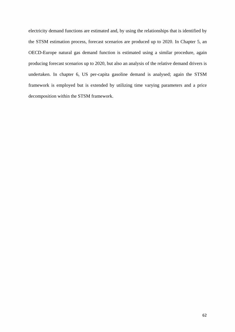
62
electricity demand functions are estimated and, by using the relationships that is identified by
the STSM estimation process, forecast scenarios are produced up to 2020. In Chapter 5, an
OECD-Europe natural gas demand function is estimated using a similar procedure, again
producing forecast scenarios up to 2020, but also an analysis of the relative demand drivers is
undertaken. In chapter 6, US per-capita gasoline demand is analysed; again the STSM
framework is employed but is extended by utilizing time varying parameters and a price
decomposition within the STSM framework.

63
CHAPTER 4: Turkish Electricity Demand∗
4.1 Introduction
This Chapter investigates the relationship between:
i) Turkish industrial electricity consumption, industrial value added (output) and
electricity prices;
ii) Turkish residential electricity consumption, household total final consumption
expenditure and residential electricity prices; and
iii) Turkish aggregate electricity consumption, GDP, and average real electricity
prices.
To achieve this, electricity demand functions for these Turkish sectors are estimated by
applying the STSM outlined in the previous chapter using annual data for the period 1960 to
2008. These relationships are then used to produce forecast scenarios for Turkish industrial,
residential, and aggregate electricity demand (and the ‘residual’ sector).
∗Earlier preliminary work for this chapter was presented at the following:
• 2ndInternational Workshop on Empirical Methods in Energy Economics (EMEE2009) Organised by CBEEDAC-SEEC-CEPE, Jasper, Alberta, Canada 28-29 August 2009;
• 10thInternational Association for Energy Economics (IAEE) European Conference ‘Energy Policies and Technologies for Sustainable Economies’, Vienna, Austria, 7-10 September 2009. where the paper was given a Best Student Paper Award; and
• The Young Energy Engineers and Energy Economists Workshop, University of Cambridge, Cambridge 8-9 April 2010.
The results from this chapter have been published in:
• ‘Industrial Electricity for Turkey: A Structural Time Series Analysis’, Energy Economics, 33, 426-436, 2011 (with L. C. Hunt);
• ‘Modelling and Forecasting Turkish Residential Electricity Demand’, Energy Policy,39, 3117-3127, 2011 (with L. C. Hunt);and
• ‘Turkish Aggregate Electricity Demand: An Outlook to 2020’, Energy, 36, 6686-6696, 2011 (with L. C. Hunt).

64
As discussed in the chapters above, for sustainable economic growth, robust reliable demand
forecasts of Turkish electricity demand are vital for the development of appropriate Turkish
energy policies. The aim of this chapter therefore is to investigate how the structural time
series methodology performs in terms of modelling Turkish electricity demand, estimating
the key elasticities, and forecasting future electricity demand.
The motivation and justification for this chapter is twofold. Firstly, the STSM approach is
utilised since this allows for a focus on the economic and exogenous factors of different
electricity demand functions by investigating the relationship between electricity
consumption, economic variables, and a UEDT. This work is therefore, as far is known, the
first that allows for a stochastic the UEDT when modelling Turkish electricity demand.
Secondly, the estimated models are used to produce forecasts of Turkish electricity demand,
which are compared to past Turkish electricity demand projections, since it is hypothesised
that a model estimated using the structural time series methodology will outperform these
previous forecasts. That is, using the STSM to underpin the forecast arguably provides one
explanation for the shortcomings of previous ‘unsuccessful’ forecasts; these forecasts being
essential for evaluating policies and strategies in order to achieve Energy Security and to
decrease CO2 emissions. Therefore, given the importance of electricity demand, this work
contributes to the development of Turkish energy policy and the strategy to ensure future
Turkish energy security. Additionally, reliable forecasts are vital for Turkish electricity
generating and distribution companies in order to establish their long-term investment
decisions. However, before investigating the electricity demand functions, it is important to
understand the history and development of the Turkish energy, which is discussed in the next
section.

65
4.2 Overview of Energy Situations in Turkey
Turkey covers an area of just over 780 thousand km2, straddling South Eastern Europe and
South Western Asia with an estimated population of just under 72 million people in 2007
(FCO, 2010). Turkey’s economy consists of modern industries, the commercial sector, and
the traditional agricultural sector. Although the Turkish economy experienced a period of
transformation from agriculture to industrial followed by a rapid urbanization, especially after
1982, the agriculture sector still accounts for 25% of total employment. The major industrial
sectors are textiles and clothing, which employ about a third of total industrial employment.
Turkey’s GDP in 2011was1.053 trillion US dollars (constant 2011PPP prices) accounting for
just over 1% of the world’s total GDP (World Fact Book, 2012; IEA, 2010b).
4.2.1 Turkish Energy History
In this section, Turkey’s energy balances are reviewed in two sub-sections. Firstly, energy
demand, production, sectoral energy consumptions development over time are reviewed and
secondly the more recent situation is analysed.
4.2.1.1 Historical Development of Turkish Energy 1960-2008
In 1960, Turkey’s total indigenous energy production was 9371 ktoe of which 5878 ktoe
(63%) was combustible renewable and waste production, 3036 ktoe (32%) was coal and coal
products production, 370 ktoe (4%) was petroleum production, and 86 ktoe (1%) was hydro
production. In 1960, there was no natural gas, geothermal, solar & wind and other energy
sources production (Figure 4.1) (IEA, 2010c).
Turkey’s domestic primary energy production reached its peak in 1998 with 29,071 ktoe. Of
this, 13943 ktoe (48%) was coal and coal products, 6980 ktoe (24%) was combustible
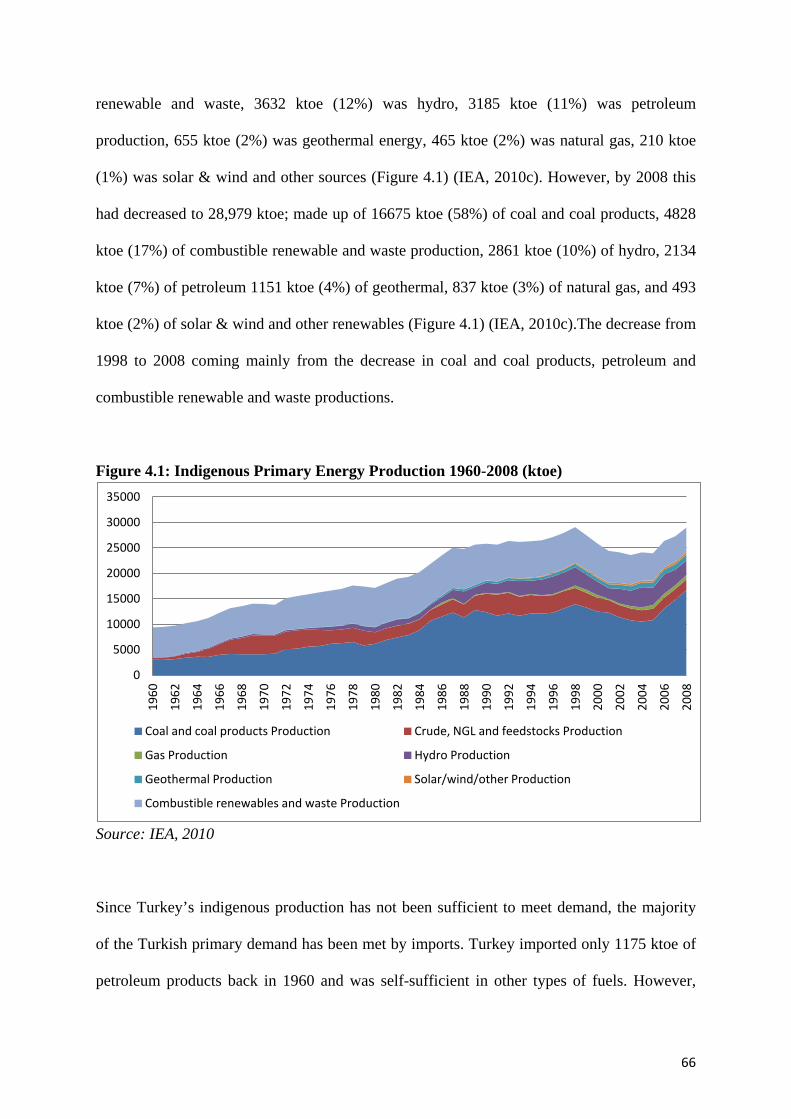
66
renewable and waste, 3632 ktoe (12%) was hydro, 3185 ktoe (11%) was petroleum
production, 655 ktoe (2%) was geothermal energy, 465 ktoe (2%) was natural gas, 210 ktoe
(1%) was solar & wind and other sources (Figure 4.1) (IEA, 2010c). However, by 2008 this
had decreased to 28,979 ktoe; made up of 16675 ktoe (58%) of coal and coal products, 4828
ktoe (17%) of combustible renewable and waste production, 2861 ktoe (10%) of hydro, 2134
ktoe (7%) of petroleum 1151 ktoe (4%) of geothermal, 837 ktoe (3%) of natural gas, and 493
ktoe (2%) of solar & wind and other renewables (Figure 4.1) (IEA, 2010c).The decrease from
1998 to 2008 coming mainly from the decrease in coal and coal products, petroleum and
combustible renewable and waste productions.
Figure 4.1: Indigenous Primary Energy Production 1960-2008 (ktoe)
Source: IEA, 2010
Since Turkey’s indigenous production has not been sufficient to meet demand, the majority
of the Turkish primary demand has been met by imports. Turkey imported only 1175 ktoe of
petroleum products back in 1960 and was self-sufficient in other types of fuels. However,
0
5000
10000
15000
20000
25000
30000
35000
1960
1962
1964
1966
1968
1970
1972
1974
1976
1978
1980
1982
1984
1986
1988
1990
1992
1994
1996
1998
2000
2002
2004
2006
2008
Coal and coal products Production Crude, NGL and feedstocks Production
Gas Production Hydro Production
Geothermal Production Solar/wind/other Production
Combustible renewables and waste Production

67
between 1960 and 2008 Turkey’s net energy imports increased to a net 69523 ktoe of energy;
made up of 21570 ktoe (31%) of crude oil, 30244 ktoe (43%) of natural gas, 12856 ktoe
(18%) of coal and coal products, and 5924 ktoe (8%) of petroleum products (Figure4.2) (IEA,
2010c).
Figure 4.2: Net Energy imports 1960-2008 (ktoe)
Source: IEA, 2010
In 1960, total final energy consumption of Turkey was 9748 ktoe, which consisted of 5878
ktoe (60%) of combustible renewable and waste, 2249 ktoe (23%) of coal and coal products,
1405 ktoe (14%) of petroleum products, 184 ktoe (2%) of electricity, and 31 ktoe (0.3%) of
natural gas. Final energy consumption increased continuously until 1978 reaching 26864
ktoe; however, following the 1978 economic crisis. Turkey’s total final consumption slightly
decreased to 25539 ktoe in 1979. After 1979, total final energy consumption continued to
increase until 1993 when it reached 45818 ktoe but decreased again in 1994 to 43603 ktoe at
the same time as the economic problems of that year. From 1994, Turkey’s total final
consumption increased again until 1998 when it reached 54300 ktoe. Again, the increase was
0
10000
20000
30000
40000
50000
60000
70000
80000
1960
1962
1964
1966
1968
1970
1972
1974
1976
1978
1980
1982
1984
1986
1988
1990
1992
1994
1996
1998
2000
2002
2004
2006
2008
Coal and coal products Net Imports Crude, NGL and feedstocks Net Imports
Oil products Net Imports Gas Net Imports

68
halted in 1999 following the economic problems, with Turkey’s total final consumption
falling to 52551 ktoe in 1999. As the economy recovered again, energy consumption
increased to 58447 ktoe in 2000, but falling again in 2001 to 52716.84 ktoe as economic
problems emerged again. From then Turkey’s total final energy consumption increased
continuously from1960 to 2007 when it reached 75450 and fell slightly in 2008 to 73365 ktoe
(Figure 4.3). In 2008,Turkey’s final energy consumption reached 73365 ktoe, consisting of
27445 ktoe (37%) of petroleum products, 13710 ktoe (19%) of electricity, 12776 ktoe (17%)
of coal and coal products, 13233 ktoe (18%) of natural gas, 4770 ktoe (7%) of combustible
renewable and waste, 1011 ktoe (1,4%) of geothermal energy, and 420 ktoe (0,6%) of solar &
wind and other energy sources (Figure 4.3) (IEA, 2010c).
Figure 4.3: Turkish Energy Consumption by Fuel 1960-2008 (ktoe)
Source: IEA, 2010
Turkey’s aggregate energy intensity did not change appreciably over the period 1960 to 2008.
In order to create 1000 $ (2000 constant PPP) of GDP in 1960, 0.11 toe was needed where in
2008 it was 0.12 (Figure 4.4). One possible reason might be that Turkey failed to implement
0
10000
20000
30000
40000
50000
60000
70000
80000
1960
1963
1966
1969
1972
1975
1978
1981
1984
1987
1990
1993
1996
1999
2002
2005
2008
Electricity
Combustible renewables and waste
Solar/wind/other
Geothermal
Gas
Oil products
Coal and coal products
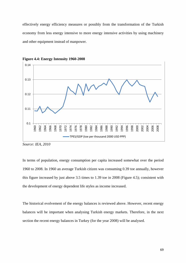
69
effectively energy efficiency measures or possibly from the transformation of the Turkish
economy from less energy intensive to more energy intensive activities by using machinery
and other equipment instead of manpower.
Figure 4.4: Energy Intensity 1960-2008
Source: IEA, 2010
In terms of population, energy consumption per capita increased somewhat over the period
1960 to 2008. In 1960 an average Turkish citizen was consuming 0.39 toe annually, however
this figure increased by just above 3.5 times to 1.39 toe in 2008 (Figure 4.5); consistent with
the development of energy dependent life styles as income increased.
The historical evolvement of the energy balances is reviewed above. However, recent energy
balances will be important when analysing Turkish energy markets. Therefore, in the next
section the recent energy balances in Turkey (for the year 2008) will be analysed.
0.1
0.11
0.12
0.13
0.14
1960
1962
1964
1966
1968
1970
1972
1974
1976
1978
1980
1982
1984
1986
1988
1990
1992
1994
1996
1998
2000
2002
2004
2006
2008
TPES/GDP (toe per thousand 2000 USD PPP)
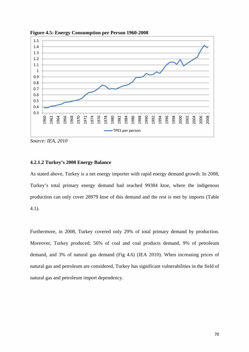
70
Figure 4.5: Energy Consumption per Person 1960-2008
Source: IEA, 2010
4.2.1.2 Turkey’s 2008 Energy Balance
As stated above, Turkey is a net energy importer with rapid energy demand growth. In 2008,
Turkey’s total primary energy demand had reached 99384 ktoe, where the indigenous
production can only cover 28979 ktoe of this demand and the rest is met by imports (Table
4.1).
Furthermore, in 2008, Turkey covered only 29% of total primary demand by production.
Moreover, Turkey produced; 56% of coal and coal products demand, 9% of petroleum
demand, and 3% of natural gas demand (Fig 4.6) (IEA 2010). When increasing prices of
natural gas and petroleum are considered, Turkey has significant vulnerabilities in the field of
natural gas and petroleum import dependency.
0.3 0.4 0.5 0.6 0.7 0.8 0.9
1 1.1 1.2 1.3 1.4 1.5
1960
1962
1964
1966
1968
1970
1972
1974
1976
1978
1980
1982
1984
1986
1988
1990
1992
1994
1996
1998
2000
2002
2004
2006
2008
TPES per person

71
Table 4.1: Turkey’s 2008 Energy Balance (ktoe)
Source Coal
and
Coa
l Pr
oduc
ts
Crud
e, N
GL,
Feed
Sto
cks
Petr
oleu
m
Prod
ucts
Nat
ural
Gas
Hydr
o
Geot
herm
al
Sola
r Win
d O
ther
Com
bust
ible
Re
new
able
s an
d W
aste
Elec
tric
ity
Tota
l
Indigenous Production 16674.70 2134.31 0 837.36 2861.22 1150.49 492.75 4827.86 0 28978.60
Imports 12856.20 21570.40 14406.00 30603.30 0 0 0 0 67.85 79503.40
Exports 0 0 -6526.81 -359.01 0 0 0 0 -96.49 -6982.31
International Marine Bunkers 0 0 -652.69 0 0 0 0 0 0 -652.69
International Aviation Bunkers 0 0 -1302.28 0 0 0 0 0 0 -1302.28
Stock Changes -70.26 -140.80 65.89 -897.83 0 0 0 0 0 -1043
Total Primary Energy Supply 29460.60 23563.90 5989.78 30183.80 2861.22 1150.49 492.75 4827.86 -28.64 98501.70
Statistical Difference 202.68 700.77 -20.68 0 0 0 0 0 0 882.76
Primary Demand 29663.20 24264.70 5969.09 30183.80 2861.22 1150.49 492.75 4827.86 -28.64 99384.50
Transfers
0 0 0 0 0 0 0
Transformation -16233.80 -24264.70 22735.20 -16452.40 -2861.22 -139.67 -72.84 -57.93 17063.90 -20283.30
Energy Industry Use -598.23 0 -1259.28 -442.42 0 0 0 0 -962.00 -3261.92
Losses -54.88 0 0 -56.13 0 0 0 0 -2363.37 -2474.38
Total Final Consumption 12776.30 0 27445.10 13232.90 0 1010.82 419.91 4769.92 13709.90 73364.90
Non Energy Use 0 0 5106.70 262.26 0 0 0 0 0 5368.96
Final Energy Consumption by Sector 12776.30 0 22338.40 12970.60 0 1010.82 419.91 4769.92 13709.90 67995.90
Industry 6120.93 0 1334.19 3194.40 0 0 125.97 0 6219.52 16995
Transport 0 0 14786.60 183.05 0 0 0 15.25 82.56 15067.40
Residential 4930.08 0 1685.73 6524.02 0 1010.82 293.94 4754.68 3404.22 22603.50
Other Final Consumers 1725.33 0 4531.87 3069.14 0 0 0 4003.64 13330
Source: IEA, 2010
Turkey’s total primary energy demand was 99385 ktoe in 2008. 20283 ktoe (20%) was
transfers and transformation, 3262 ktoe (3%) was energy industries own consumption, 2474

72
ktoe (3%) was lost during the distribution and transportation process, and 73365 ktoe (74%)
went to final consumption (Figure 4.7) (IEA, 2010c). Of this total final consumption the
industrial sector consumed 16995 ktoe (25%), the transport sector consumed 15067 ktoe
(22%), the residential sector consumed 22604 ktoe (33%), and the other sectors consumed
13330 ktoe (20%) in 2008 (IEA, 2010c).
Figure 4.6: Turkey’s Energy Demand, Production, and Net Imports 2008 (ktoe)
Source: IEA, 2010
Figure 4.7: The Allocation of Primary Energy Demand 2008
Source: IEA, 2010
0
10000
20000
30000
40000
50000
60000
70000
80000
90000
Coal and Coal Products Crude, NGL, Feed Stocks Natural Gas Total
Indigenous Production Primary Demand Net Imports
20%
3% 3%
74%
Transformation
Energy Industry Use
Losses
Final Consumption

73
Furthermore, Turkey’s total final energy consumption of 73365 ktoe in 2008 was made up of
the following energy types: petroleum products 27445 ktoe (33%); electricity 13710 ktoe
(20%); coal and coal products 12776 ktoe (19%); natural gas 13233 ktoe (19%); combustible
renewable and waste 4770 ktoe (7%); geothermal energy 1011 ktoe (1%); solar & wind 420
ktoe (1%); and other source of energy (Figure 4.8) (IEA, 2010c). However, the distribution of
different energy types differs somewhat in the different sectors. Out of a total of 16695 ktoe
of energy in 2008 consumed by the Turkish industrial sector, 6121 (36%) ktoe was coal and
coal products, 6220 ktoe (36%) was electricity, 1334 (8%) ktoe was petroleum products,
3194 ktoe (19%) was natural gas, and 126 ktoe (1%) was solar & wind and other sources
(Figure 4.9) (IEA, 2010c).
Figure 4.8: Energy Consumption by Fuel 2008
Source: IEA, 2010
19%
33% 19%
1% 1%
7%
20%
Coal and Coal Products
Petroleum Products
Natural Gas
Geothermal
Solar Wind Other
Combustible Renewables and Waste
Electricity

74
Figure 4.9: Industry Sector Energy Consumption by Fuel 2008
Source: IEA, 2010
For the Turkish residential sector, which consumed a total 22604 ktoe in 2008, 4755 ktoe
(21%) was combustible renewable and waste, 6524 ktoe (29%) was natural gas, 1686 ktoe
(7%) was petroleum products, 3404 ktoe (15%) was electricity, 4930 ktoe (22%) was coal
and coal products, 1011 (5%) was geothermal energy, and 294 (1%) was solar & wind and
other energy sources (Figure 4.10) (IEA, 2010c).Whereas for the Turkish transport sector,
which consumed 15067 ktoe energy in 2008, 14787 ktoe (98%) was petroleum products, 83
ktoe (1%) was electricity, and 183 ktoe (1%) was natural gas (IEA, 2010c).
The other sector (i.e. the total less industrial, residential and transport) consumed a total of
13330 ktoe energy in 2008, of which 4532 ktoe (34%) was petroleum products, 4004 ktoe
(30%) was electricity, 1725 ktoe (13%) was coal and coal products and 3069 ktoe (23%) was
natural gas (IEA, 2010c).
36%
8% 19%
1%
36% Coal and Coal Products
Petroleum Products
Natural Gas
Solar Wind Other
Electricity

75
Figure 4.10: Residential Sector Energy Consumption by Fuel 2008
Source: IEA, 2010
The above has given an overview of the history and current energy situation in Turkey before
focussing the energy source that is modelled in this chapter, Electricity. The next section
therefore discusses the historical development of Turkish electricity.
4.3 Development of Turkish Electricity Markets
The first attempt to produce electricity in Turkey was during the Ottoman Empire era at the
beginning of the 20th century. In 1902, electricity was first generated and distributed to
households by connecting a 2 KW dynamo to a watermill. Technical knowledge at that time
was limited; therefore, the Ottoman Empire targeted foreign investment in order to finance
electricity generation. To help facilitate this, the ‘Privileges for Public Wealth’ law was
introduced in 1910, giving privileges to electricity generation companies such as the
Hungarian Ganz Partnership that, with a Hungarian and Belgium bank, established the
‘Ottoman Electricity Stock Company’. As a result, in 1913 the first large scale electricity
22%
7%
29% 5% 1%
21%
15%
Coal and Coal Products
Petroleum Products
Natural Gas
Geothermal
Solar Wind Other
Combustible Renewables and Waste
Electricity

76
power plant (13.4 MW) was built in Silahtaraga, Istanbul. This was followed by construction
of further power plants in Anatolia (Dolun, 2002 and TEK, 1972).
When the Turkish Republic was founded in 1923, the installed electricity capacity for Turkey
was 33 MW with production around 50 million kWh. The privileged contracts for foreign
electricity generation companies were approved by the new Turkish Republic Administration,
but only for a temporary period, acknowledging the lack of technological knowledge within
Turkey at that time. The privilege contracts were designed to favour generation companies by
indexing the electricity prices to gold prices. Given this, electricity prices were high in the
early republican era leading to some electricity intensive industrial factories building their
own power generation facilities. This allowed them to produce electricity for their own use
and to supply to local households located nearby these facilities23 (Dolun, 2002 and TEK,
1972).
Given that the foreign private firms involved in the Turkish electricity industry at this time
aimed at maximising profits, they were reluctant to invest in rural areas, thus slowing down
both the increase in electricity generation and electrification. Therefore, the Etibank (a
governmental entrepreneurship) was established in 1935 to operate in the electricity
generation and mining sectors. In the same year the Electric Power Resources and Survey
Administration was also established with the remit to examine electricity generation
opportunities from hydro and other fuels. In addition, starting in 1938 thru 1944 the power
plants operating under the control of the foreign concessionary private companies were
bought by the Turkish government and were given to the municipal administrations for
23 For example, the Karbuk Iron and Metal Factory and the Izmit Seka and Sumerbank were also known as auto-producers (Dolun, 2002 and TEK, 1972).

77
management. Furthermore, in 1957, the Turkish government established a new organization
namely the Energy and Natural Resources Department, responsible for coordinating the
activities of electricity generation and distribution companies and the Ministry of Energy and
Natural Resources was founded in 1963 to administer Turkish energy policies (Dolun, 2002
and TEK, 1972).
In 1970, the Turkish Electricity Institution (TEI)24 was established with the main aim of
coordinating electricity generation across the country. 25 Consequently, the TEI had a
monopoly in the generation and transmission of electricity, with distribution undertaken by
municipal administrations. However, following the introduction of Law No 2705 in 1982, the
distribution function of the municipal administrations was transferred to the TEI giving
Turkey a fully vertically integrated state owned monopoly (Dolun, 2002). In 1993, Law no.
513 was introduced, with the stated aim to privatize the TEI. Following this, the TEI was
divided into two state owned enterprises, the ‘Turkish Electricity Generation and
Transmission Co. (TEGTC)26’ and the ‘Turkish Electricity Distribution Co. (TEDC)27’ but
their relationship with the Ministry of Energy and Natural Resources was maintained as
before (Dolun, 2002).
In 2001, the Electricity Market Law No. 4628 was introduced, with the aim of regulating the
electricity market with the establishment of the Regulatory Body of Electricity Market in the 24 In Turkish this is known as, TEK (Turk Elektrik Kurumu) translated by author.
25 Although at different times, similar developments occurred across Western Europe (although often for similar reasons) resulting in the establishment of centralised electricity industries and institutions, coupled with nationalization. For example, Electricite de France in France in the mid 1940s, the Central Electricity Generating Board in the UK in the late 1950s and the Ente Nazionale per l'Energia Elettrica (ENEL) in Italy in the early 1960s.
26 In Turkish this is known as TEAS (Turkiye Elektrik Anonim Sirketi) translated by author.
27 In Turkish this is known as TEDAS (Turkiye Elektrik Dagitim Anonim Sirketi) translated by author.

78
same year. Furthermore, the TEGTC was restructured, being divided into three state owned
public enterprises, the ‘Turkish Electricity Transmission Co. (TETC) 28 , the ‘Turkish
Electricity Generation Co. (TEGC)29, and the ‘Turkish Electricity Trading Co. (TETC)30’.
Within this new structure TEGC took over and operated the public power plants, TETC was
given responsibility for wholesale operations and became the holder of all pervious Build-
Own-Operate (BOO), Build-Operate-Transfer (BOT) and Transfer of Operating Rights
(TOOR) agreements and long term power purchase agreement with Treasury guaranties.
TETC was assigned responsibility for transmission and balancing and settlement procedure in
order to balance power operation between parties, covering both the physical and financial
aspects of transmission operation; hence, TETC became the transmission system operator for
Turkey (Dolun, 2002).
The history and development of the Turkish electricity industry, discussed above, has been
driven by past governments’ concerns with meeting the growth in electricity demand in order
to maintain economic growth and raise the living standards of the Turkish people. This
remains true for the present Turkish government. Therefore, given that the Turkish electricity
industry remains under state control, with only, limited genuine market activity, it is vital that
Turkish policy makers understand the main characteristics and the key drivers of both past
and future of electricity demand. This is therefore one of the key motivations for undertaking
the research for this thesis; it aims to identify and forecast Turkish electricity demand.
However, before this is undertaken, Turkish Economy and Electricity consumption over the
period 1960-2008 will be analysed in the next section.
28 In Turkish this is known as TEIAS (Turkiye Elektrik Iletim Anonim Sirketi) translated by author.
29 In Turkish this is known as EUAS (Elektrik Uretim Anonim Sirketi) translated by author.
30 In Turkish this is known as TETAS (Turk Elektrik Ticaret ve Taahut Anonim Sirketi) translated by author.

79
4.4 Turkish Economy and Electricity Consumption 1960-2008
The Turkish economy experienced a number of economic crises and economic policy
changes during the period 1960-2008. In particular, there were four serious and long lasting
economic crises in 1978-1981, 1988-1989, 1994 and 1998-2002; in addition to the three mid-
size, and relatively short lasting, economic crises in 1969, 1982, and 1991 (Kazgan, 2002).
As part of the response to these continuing problems, the Turkish government responded in
the 1960s and 1970s by implementing an industrialization strategy based upon import
substitution. This resulted in significantly higher and more stable growth rates until the late
1970s. However, the Turkish government’s decision not to allow the increase in the cost of
oil imports due to the oil price hikes of the early and late 1970s to permeate through the
economy and hence shoulder the true economic ‘burden’ of high oil prices resulted in balance
of payments problems and an increase in the budget deficit. This led to the worst political
instability in Turkish history, when inflation reached 64% with a balance of payments ‘crisis’
in 1979, with GDP declining in both 1979 and 1980. It was following this period that Turkey
adopted export-oriented industrialization policies (Taymaz and Yilmaz, 2007).
Not surprisingly, these crises and policy changes affected both industrial output and industrial
electricity consumption. As highlighted above, before 1980 the Turkish economy was inward
looking with an import-substituting industrialization strategy; whereas, after 1980 this
changed to an export oriented industrialization strategy. Therefore, before 1980 the Turkish
industrial sector was more vulnerable to domestic shocks whereas after 1980 it became more
vulnerable to external shocks such as the Gulf War and the global economic crisis. However
despite this volatility, Turkish industrial electricity consumption increased by an average of
about 8½% per year from about 1½ TWh to just over 72 TWh over the period 1960 to 2008

80
(IEA, 2010c). This high growth rate of industrial electricity consumption would appear,
according to Bakirtas et al. (2000) to be mainly a result of the increasing number of
applications of energy intensive technologies in the Turkish industrial sector.
Although Turkish industrial electricity consumption generally followed an upward trend over
the period 1960 to 2008 some falls did occur; consistent with the economic crises, namely
just under 4% in 1991, just under 2.4% in 2001, and a very marginal fall in 1994 (IEA,
2010c). In 2008, industrial electricity consumption accounted for 45% of total Turkish
electricity consumption, down from just above two thirds in 1960. Although the share of
industrial electricity consumption in total electricity consumption diminished, it still has a
significant weight in overall electricity consumption (IEA, 2010c). On the other hand
industrial value added increased from just under 9 billion (2005 constant YTL) to just under
175 billion (2005 constant YTL) representing an average annual increase of just under 6½%
for the period 1960 to 2008 as illustrated in Figure 4.11 (World Bank, 2010). As discussed
above, the effect of the changing international oil price and energy prices in general were not
felt directly throughout the economy, including the industrial sector, given the regulation of
energy prices by the Turkish government.
In 1970 just over 50% of the Turkish population benefited from accessing electricity but by
1987 it had almost reached 100% (Altas et. al., 1994). In the early part of this period,
electricity was generally used for lightening but use expanded for a range of other household
energy services in the latter part with the installation of new appliances such as TVs,
refrigerators, etc. It is commonly expected that higher household income and expenditure will
result in higher demand for the services emanating from these kinds of appliances, which use
electricity. In the short term, this is likely to boost electricity consumption but in the longer

81
term, higher income is likely to result also in households replacing appliances that use old
technologies with new more efficient ones that might have a lessening effect on electricity
consumption. It is therefore important for policy makers and planners to have some idea of
the short and long run income and expenditure elasticities.
Figure 4.11: Industrial Value Added, Industrial Electricity Consumption, Industrial Electricity Prices Growth Rates 1960-2008
From 1960 to 2008, Turkish residential electricity consumption increased by an average of
about 10% per year, from 0.5 TWh to 39.5 TWh (IEA, 2010c). Whereas from 1960 to 2008
household total final expenditure increased on average by just under 5% per year, from about
53 billion YTL (2005 Constant YTL) to just over 500 billion YTL (2005 constant YTL)
(World Bank, 2010). Furthermore, over the period 1960 to 2008 electricity prices were
mostly controlled by successive Turkish governments despite the Electricity Market Law No.
4628 introduced in 2001 with the aim of creating a liberalized market structure, as discussed
above; hence, real electricity prices decreased by an average of about 1% per annum over the
1960 1965 1970 1975 1980 1985 1990 1995 2000 2005 2010
-20
-10
0
10
20
30
40
%% Change in Turkish Industrial Electricity Consumption % Change in Real Turkish Industrial Value Added (2005=100)
% Change in Real Turkish Industrial Electricity Prices (2005=100)
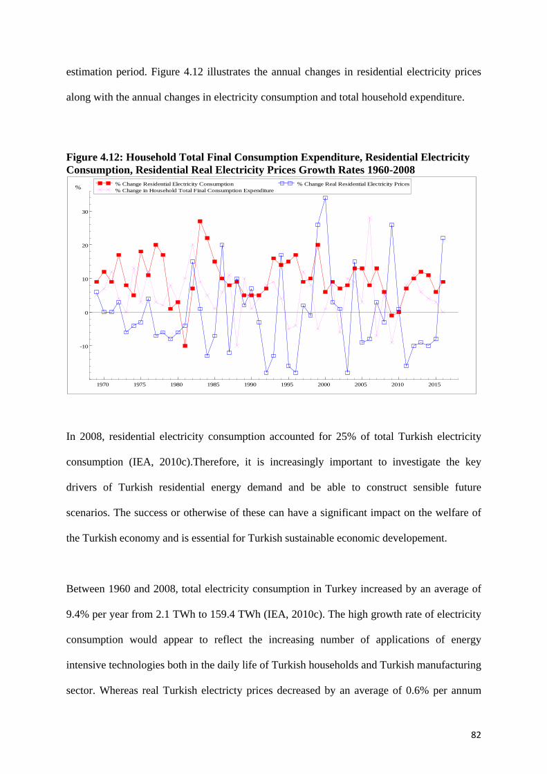
82
estimation period. Figure 4.12 illustrates the annual changes in residential electricity prices
along with the annual changes in electricity consumption and total household expenditure.
Figure 4.12: Household Total Final Consumption Expenditure, Residential Electricity Consumption, Residential Real Electricity Prices Growth Rates 1960-2008
In 2008, residential electricity consumption accounted for 25% of total Turkish electricity
consumption (IEA, 2010c).Therefore, it is increasingly important to investigate the key
drivers of Turkish residential energy demand and be able to construct sensible future
scenarios. The success or otherwise of these can have a significant impact on the welfare of
the Turkish economy and is essential for Turkish sustainable economic developement.
Between 1960 and 2008, total electricity consumption in Turkey increased by an average of
9.4% per year from 2.1 TWh to 159.4 TWh (IEA, 2010c). The high growth rate of electricity
consumption would appear to reflect the increasing number of applications of energy
intensive technologies both in the daily life of Turkish households and Turkish manufacturing
sector. Whereas real Turkish electricty prices decreased by an average of 0.6% per annum
1970 1975 1980 1985 1990 1995 2000 2005 2010 2015
-10
0
10
20
30
% % Change Residential Electricity Consumption % Change in Household Total Final Consumption Expenditure
% Change Real Residential Electricity Prices
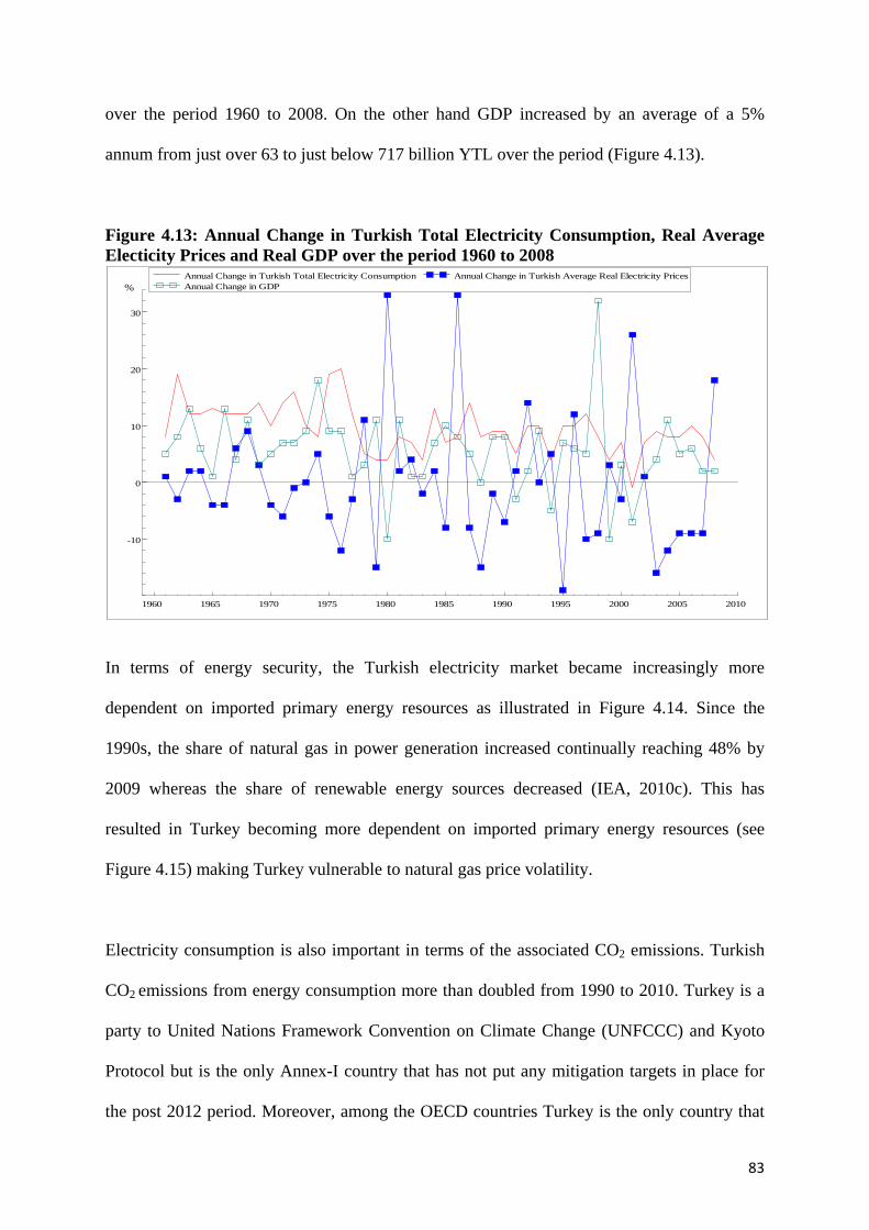
83
over the period 1960 to 2008. On the other hand GDP increased by an average of a 5%
annum from just over 63 to just below 717 billion YTL over the period (Figure 4.13).
Figure 4.13: Annual Change in Turkish Total Electricity Consumption, Real Average Electicity Prices and Real GDP over the period 1960 to 2008
In terms of energy security, the Turkish electricity market became increasingly more
dependent on imported primary energy resources as illustrated in Figure 4.14. Since the
1990s, the share of natural gas in power generation increased continually reaching 48% by
2009 whereas the share of renewable energy sources decreased (IEA, 2010c). This has
resulted in Turkey becoming more dependent on imported primary energy resources (see
Figure 4.15) making Turkey vulnerable to natural gas price volatility.
Electricity consumption is also important in terms of the associated CO2 emissions. Turkish
CO2 emissions from energy consumption more than doubled from 1990 to 2010. Turkey is a
party to United Nations Framework Convention on Climate Change (UNFCCC) and Kyoto
Protocol but is the only Annex-I country that has not put any mitigation targets in place for
the post 2012 period. Moreover, among the OECD countries Turkey is the only country that
1960 1965 1970 1975 1980 1985 1990 1995 2000 2005 2010
-10
0
10
20
30
%Annual Change in Turkish Total Electricity Consumption Annual Change in GDP
Annual Change in Turkish Average Real Electricity Prices

84
does not have a national emission target for 2020 (IAE, 2010). Consequently, Turkey might
well face future international pressure to set emission targets. In the short term, the Turkish
government’s priority is to meet growing energy demand, but in the long term, ignoring these
global trends might be costly both politically and economically. However, in order to reach a
balance between securing electricity supply to meet demand and transforming the power
generation to a more sustainable level, the Turkish government requires sound and reliable
electricity demand projections to underpin their planning activities. However, as stated above,
this has not always been the case, so that given electricity consumption has been increasing
significantly, it is important that Turkish policy makers understand what drives electricity
demand and more importantly how it will evolve over the next 10 years or so.
Figure 4.14: Share of Fuels in Power Generation
Source: IEA 2010
55
33
26
35 31 29
8
30 25
7 7 5
37 37
49
40
25
18 18
37
48
0%
10%
20%
30%
40%
50%
1960 1970 1980 1990 2000 2008
Coal Petroleum Products Renewables Natural Gas

85
Figure 4.15: Self Sufficiency Vs Import Dependency
Source: IEA, 2010
In order to investigate the key drivers of Turkish industrial, residential, and aggregate
electricity demand and be able to construct sensible future scenarios, these demand functions
are estimated by utilizing STSM. In the next section, previous Turkish electricity demand
studies are reviewed in the next section.
4.5 Previous Turkish Electricity Demand Forecast Studies
Studies before the 1970s that directly focused on analysing Turkish electricity demand are
very limited, being generally carried out by governmental institutions with their own
approaches, namely the State Planning Organization (SPO), the State Institute of Statistics
(SIS) and the Ministry of Energy and Natural Resources (MENR). Although some research in
those institutions tried to apply mathematical modelling techniques to analyse energy demand
in the late 1970s, these methods were not used in official energy planning until 1984. Before
93% 83%
76% 69%
45% 36%
7% 17%
24% 31%
55% 64%
0%
10%
20%
30%
40%
50%
60%
70%
80%
90%
100%
1960 1970 1980 1990 2000 2008
Self Sufficeny Import Dependency
86
1984, national energy policy was shaped by the forecasts of the SPO in which they employed
various simple best-fit curves (Ediger and Tatlidil, 2002).
The MENR utilized different models in order to determine energy demand functions and to
make future projections. For instance, ‘Balance’ models that are non-linear equilibrium
models that match the energy demand with available resources and technologies and ‘Impact’
models that focus on the relation between energy consumption and its interaction with the
environment were employed in the framework of Energy and Power Evaluation Program
(ENPEP). Both models were used for the long-term supply and demand projections between
1981 and 1985. The MENR began to use the simulation models namely MAED, WASP III,
and EFOM-12 C Mark. MAED (Model for Analysis of Energy Demand) and WASP III
(Wien Automatic System Planning) were originally developed by the International Atomic
Energy Agency (IAEA) and the energy demand model EFOM-12 C Mark (Energy Flow
Optimization Model) was developed by the commission of the European Union starting from
1984 (Ediger and Tatlidil, 2002).
At the same time, SPO also developed its own models based on sectoral energy demand for
different consumer groups, subgroups and finally the mathematical models were developed
for each sub group by regression. On the other hand, the SIS explored the relationship
between demographic factors and economic parameters with energy demand in its models.
Both of the models explored by SIS and SPO verified the relationship between energy
demand and GDP (Ediger and Tatlidil, 2002).
The previous forecast and energy modelling studies above used different kinds of approaches,
but the main motivation of all those studies was to provide better energy and electricity

87
planning tools for policy makers for sustainable economic growth. However, the previous
forecast studies such as those produced from MAED, WASP III, and EFOM-12 C Mark,
always predicted much higher demand levels than the actual outturn. As an example the
official total electricity demand projections for 2003 produced in 1987, 1990, 1993, 1996 and
2000 (utilizing the MAED) are illustrated in Figure 4.16, which demonstrates the ‘over
forecasts’ (TETC, 2009). According to Keleş (2005), this is mainly due to “technical
deficiencies of the models used, lack of ability of the relevant authorities in creating precise
assumptions and not having transparency and accountability in the relevant processes” (p. vi).
Moreover, Keleş (2005) argues that the policies adopted based upon these unsuccessful
forecasts resulted in a significant proportion of electricity generation capacity remaining idle,
transformed the Turkish economy to be more dependent on imported primary energy
resources, prevented energy markets liberalization, and resulted in high electricity prices.
Furthermore, Ediger and Tatlidil (2002) stated that the values of the future predictions of
demographic and economic variables used in the MAED models by SPO were significantly
manipulated by government policies in line with high economic growth targets rather than
reliable forecasts.
In summary, the above has illustrated how previous projections of Turkish electricity demand
generally proved to be above that actually observed (i.e. they ‘over-forecast’). This mislead
Turkish policy makers, causing them to implement projects to meet this perceived demand
that later proved to be incorrect. This resulted in ‘short-term’ policy decisions with the
installation of gas fuelled power plants rather than ‘longer-term’ policy decisions such as to
install power plants fuelled by renewable energy. As a result, the share of natural gas in
power generation and dependency to imported natural gas gradually increased.

88
Hence, as explained above, a key motivation for this chapter is to develop a more robust
model of Turkish energy demand in order to produce more reliable forecasts and scenarios
for future electricity demand, which is undertaken below but it is important beforehand to
consider previous academic (and other) work on Turkish electricity demand. The next section
therefore reviews these past studies.
Figure 4.16: Official Turkish Energy Demand Projections for the year 2003
Source: TETC (2009)
4.6 Previous Turkish Energy Demand Studies
There was a large increase in the number of Turkish energy modelling studies after the late
1990s and they can be divided into three main groups. In the first group, the focus is on
investigating the causality between energy consumption and economic variables (termed
‘Causality Studies’ below). In the second group, the focus is on identifying the relationship
and the magnitude of the key relationships (mainly the elasticities) between economic
variables and energy demand (termed ‘Relationship Studies’ below). Moreover, in the third
group, the aim is to forecast future energy demand using a number of different approaches
100
120
140
160
180
200
220
1987 1990 1993 1996 2000
Year Projection was Made
2003 Actual Consumption (140.9 TWh)
TWh
44% 37%
25% 21% 17%

89
(termed ‘Forecast Studies’ below). Turkish energy demand studies are briefly reviewed
below in a general context with a detailed summary presented in Table 4.2, followed by a
more detailed discussion of the studies that focus explicitly on modelling Turkish electricity
consumption.
• Causality Studies: The focus is whether statistical causality (usually defined
as Granger Causality) between energy consumption and economic variables,
such as GDP exists. These include, Erdal, et al. (2008), Karanfil (2008),
Erbaykal (2008), Jobert and Karanfil (2007), Soytas and Sari (2007), Lise and
Montfront (2007), Altinay and Karagol (2005) who applied different
techniques including simple Granger Causality, Vector Auto Regression
(VAR), Instantaneous Causality, Bonds Testing co-integration, Johansen co-
integration, Pair-wise Granger Causality, Error Variance Decomposition,
Impulse Response and Vector Error Correction Model (VECM). However,
whatever techniques were applied, all studies in this group aimed to determine
whether causality between energy consumption and certain economic
variables exists plus the direction of the causality.
• Relationship Studies: The focus is generally on identifying the relationship
between energy, activity, and price variables and the magnitude of the
relationship. These include Bakirtas et al. (2000), Erdogdu (2007), and
Halicioglu (2007) who employed different methods such as Engle-Granger
two-step procedure, Auto Regressive Moving Average, Bonds Testing Co-
integration and the Partial Adjustment Model, to estimate price and income
elasticities for total Turkish electricity demand and residential electricity
demand.

90
• Forecast Studies: Here the focus is on predicting future energy demand such
as Kavaklıoglu et al. (2009), Ediger and Akar (2007), Hamzacebi (2007),
Erdogdu (2007), Akay and Atak (2006), Ceylan and Ozturk (2004), Ozturk et
al. (2005) and Ediger and Tatlidil (2002). These studies used various methods
including Univariate Cycle Analysis, Genetic Algorithm Approach, Grey
Prediction with Rolling Mechanism, Auto Regressive Integrated Moving
Average (ARIMA), and Artificial Neural Networks.
Table 4.2: Summary of Previous Turkish Energy Demand Studies Reference Focus of Study Method Summary Kavalioglu et al. (2009)
Total Electricity Demand
Artificial Neural Networks
Turkish total electricity consumption would reach 240 TWh by 2020.
Erdal, et al. (2008)
Energy Consumption and Growth
Johansen co-integration, Pair-wise Granger causality
Energy consumption and GNP are co-integrated and there is bidirectional causality running from energy consumption and GNP and vice versa.
Karanfil (2008)
Energy Consumption, Growth and Unrecorded Economy
VECM-VAR There is a long term equilibrium relationship between the officially calculated GDP and energy consumption. However when unrecorded economy is taken into account there is no causality between energy consumption and GNP.
Erbaykal (2008)
Oil and Electricity Consumption and Economic Growth
Bounds testing co-integration approach
Both electricity and oil consumption have a short term effect on economic growth.
Soytas and Sari (2007)
Industrial Electricity Consumption
Error Variance Decomposition & Impulse Response
Industrial Value added, industrial electricity consumption, labour and fixed investment are co-integrated in long term, no significant impact on each other in short term
Hamzacebi (2007)
Total and Sectoral Electricity Consumption
Artificial Neural Networks
The total electricity consumption will reach to 500 TWh by 2020 where industrial, residential, agricultural and transport sector electricity consumption are forecasted 219TWh, 257 TWh, 20 TWh, and 4 TWh respectively.

91
Erdogdu (2007)
Electricity Consumption per capita
Partial Adjustment Model & ARIMA
Long term and short Term price elasticities are -0.04 and -0.030 respectively, income elasticity is 0.06 in short term and 0.41 in the long term. Electricity consumption is projected to reach to 160 TWh by 2014
Ediger and Akar (2007)
Primary Energy Consumption
ARIMA In the low case scenario the total primary energy consumption is projected to be 135.896 mtoe and in the high case scenario it will reach to 152.285 mtoe by 2020
Halicioglu (2007)
Residential Electricity Consumption per capita
Bounds testing co-integration Approach
Long term and short term price elasticities are varying -0.52 to -0.63 and -0.33 to -0.46 respectively and where long term and short term income elasticities varying 0.49 to 0.70 and 0.37 to 0.44 correspondingly according to lag criteria. Urbanization rate is a significant factor and has a 0.04 and 0.90 effects in the long term and in the short term respectively.
Jobert and Karanfil (2007)
Sectoral Energy Consumption by Source and Growth
Granger Causality- Instantaneous Causality
There is no evidence of a long term relationship between energy and income. They appear to be neutral with respect to each other. Strong evidence is found for instantaneous causality between variables.
Lise and Montfront (2007)
Electricity Consumption and Economic Growth
Granger Causality The causality is running from GDP to Energy consumption
Akay and Atak (2006)
Total and Industrial Electricity Consumption
Grey Prediction with Rolling Mechanism
It is projected that industrial and total consumption will be 140.37 and 265.7 TWh in 2015 respectively.
Altinay and Karagol (2005)
GDP and Energy Consumption
VAR and Granger Causality
Unidirectional causality running from electricity consumption to income
Ozturtk and Ceylan (2005)
Total Energy Consumption
Genetic Algorithm Approach
Genetic algorithm approach might be a better estimation method when it is compared with MAED projections of MENR.
Ozturk et al. (2003)
Total Electricity Consumption
Genetic Algorithm Approach
Genetic algorithm approach might be a better estimation method when it is compared with MAED projections of MENR.
Ediger and Tatlidil (2002)
Primary Energy Demand
Univariate cycle analysis
The primary energy demand will reach 130 mtoe by 2010
Bakirtas et al. (2000)
Total Electricity Consumption per capita
Engle-Granger two step procedure & ARMA
Insignificant price elasticity. Income elasticity, 0.7 short run and 3.1 long run.

92
Soytas and Sari (2007) focused on the relationship between economic activity and industrial
electricity demand for Turkey. Using annual data for 1968 to 2002, employing co-integration
Granger causality tests, Soytas and Sari (2007) explored the relationship between Turkish
industrial value added and industrial electricity consumption, whilst accounting for labour
and fixed investment. Whilst they found that all these variables are co-integrated, they found
only uni-directional causality from electricity consumption to value added. However,
arguably one criticism of this research is the failure of Soytas and Sari (2007) to include
industrial electricity prices in the model, which might explain the results obtained, and hence
the outcome arguably does not enlightening Turkish policy makers very much.
Halicioglu (2007) investigated Turkish residential electricity demand using the Bounds
Testing approach and found a range of estimated elasticities depending upon the number of
lags chosen, such as:
- Short and long run price elasticities of -0.33 and -0.52 respectively.
- Short and long run income elasticities of 0.44 and 0.70 respectively.
Halicioglu (2007) argues that the urbanization rate is also a significant variable in
determining Turkish residential energy demand finding estimated urbanization short run and
long run elasticities of 0.90 and 0.04 respectively. He also finds that the short run income and
price elasticities are lower than the long run elasticities and argues that policy makers should
consider this when implementing policy. He claims that in the short term the response to
policy changes will be limited because of the fixed energy appliances.
Although Halicioglu (2007) contributes significantly to the exploration of the residential
sector electricity demand modelling, it can arguably be improved in two main ways. Firstly,
Halicioglu (2007) uses an energy price index rather than real electricity prices. Secondly,
93
Household Total Final Expenditure probably represents household consumption capability
better than Gross National Product per capita, which Halicioglu uses.
Bakirtas et al. (2000) using price, income, population and energy consumption data over the
period 1962 to 1996, investigated the long run economic relationship between total electricity
demand per capita, income per capita and prices by using the Engle and Granger two-step
procedure and the Johansen procedure. However, they failed to find a significant price effect
and stated that this was to be expected given electricity prices were subsidised by various
Turkish governments. Nonetheless, it would not appear that this is the reason given the
degree of variability in Turkish real electricity prices, historically being somewhat more
variable (and higher) than general European real electricity prices, as illustrated in Figure
4.17. On the other hand, Bakirtas et al. (2000) concluded that the short and long run income
per capita elasticities were about 0.7 and 3.1 respectively. Furthermore, as a separate
exercise, Bakirtas et al. (2000) undertook a univariate ARMA process in order to forecast
future Turkish electricity consumption between 1997 and 2010 and concluded that aggregate
electricity consumption per capita would reach about 2222 KWh in 2010 (Bakirtas et al.,
2000).
Erdogdu (2007) also took a ‘two part’ approach to estimation and forecast. In the first part,
the Partial Adjustment Model (PAM) was employed with quarterly data including real GDP
per capita, price, and net total electricity consumption per capita between 1984 and 2004.
Erdogdu (2007) found that the short and long run price elasticities were -0.04 and -0.30
correspondingly and that the short and long run income elasticities were 0.06 and 0.41
respectively. However, Erdogdu states “data on net electricity consumption, population and
GDP is not available quarterly” hence the annual series on these data were “converted into

94
quarterly data by linear interpolation so as to make use of them together with quarterly data
on electricity prices” (Erdogdu, 2007, p. 1134). This might have helped to overcome lack of
data and observations problems, but arguably introduces an ‘artificial data generating
process’ given three out of the four series used (including the dependent variable) had an
artificial seasonal pattern imposed an might have led to biased estimated elasticities.31
Figure 4.17: Industrial and Residential Electricity Price Comparison of OECD-Europe and Turkey 1978-2008 (2005 constant US $ PPP / Kwh)
Source: IEA, 2010
In the second part, Erdogdu (2007) estimated a simple ARIMA model with annual data from
1923 to 2004 in order to construct the forecast of future Turkish electricity consumption. He
31 For example, GDP fluctuates seasonally and electricity-using appliances are likely to differ seasonally; hence, the simple linear interpolation is likely to ignore these seasonal fluctuations and hence, is likely to have led to the misidentification of the electricity demand relationship.
1980 1985 1990 1995 2000 2005 2010
0.1
0.2
2005
US
$ (P
PP)/
kwh
OECD Europe Industrial Real Electricity Prices Turkey Industrial Real Electricity Prices
1980 1985 1990 1995 2000 2005 2010
0.15
0.20
0.25
2005
US
$ (P
PP)/
kwh
OECD Europe Residential Real Electricity Prices Turkey Residential Real Electricity Prices
95
concluded that electricity consumption would increase by 3.3% per year until 2014 reaching
about 156 TWh in 2010 and about 160 TWh in 2014 (Erdogdu, 2007).
As discussed above, both Erdogdu (2007) and Bakirtas et al. (2000) attempt to explain past
electricity demand by exploring the relationship and/or causality between income, total
electricity consumption and electricity prices by using the PAM, the Johansen procedure and
the Engle and Granger two step procedure. It is somewhat surprising, therefore, that to
produce their forecasts these relationships are ignored, instead preferring to predict the future,
they both used univariate models, as described above. This is arguably a weakness in their
approach, which this research attempts to correct.
Hamzacebi (2007) used 1970-2004 sectoral electricity consumption data and Artificial Neural
Networks method to forecast the total, residential, and industrial electricity consumption.
Hamzacebi (2007) suggest that by 2020:
i) Residential electricity consumption will reach about 257 TWh.
ii) Total electricity consumption will reach about just below 500 TWh.
iii) Industrial electricity demand will reach just less than 220 TWh.
Akay and Atak (2006) using the Grey Prediction with Rolling Mechanism, focused on
forecasting Turkish industrial and total electricity demand. Akay and Atak (2006) argued
that the industrial and total electricity consumption will be about 140 TWh and just below
266 TWh correspondingly by 2015.
96
However, both Akay and Atak (2006) and Hamzacebi (2007) could arguably be criticised for
their failure to take account of the electricity price and economic activity in driving future
electricity demand – which might result in forecasts being somewhat different from outturn.
Ozturk and Ceylan (2005) utilized the Genetic Algorithm approach with data over the period
1980 to 2003 for total electricity consumption, population, imports, exports and GDP data.
Nevertheless, despite identifying a number of economic variables their interaction with
electricity consumption is not clearly defined; moreover, the effect of electricity prices was
neglected. Ozturk and Ceylan (2005) concluded that total electricity consumption would be
between about 462 TWh and 500 TWh in 2020 (Ozturk and Ceylan, 2005).
Kavaklioglu et al. (2009) employed the variables population, GDP, imports and exports in an
artificial neural network model and concluded that the Turkish total electricity consumption
would reach 240 TWh by 2020. However, the interaction of the economic variables and the
electricity consumption is not identified clearly by Kavaklioglu et al. (2009); moreover, once
again the effect of electricity prices on electricity demand is ignored (Kavaklioglu et al.,
2009).
By using only previous years’ electricity consumption values in their forecasts without
allowing for any economic demand relationship, Erdogdu (2007), Hamzacebi (2007), Akay
and Atak (2006) and Bakirtas et al. (2000) ignore the important interaction between energy
demand and economic variables in their forecasts and take into account only past electricity
consumption. On the other hand, Ozturk and Ceylan (2005) and Kavaklioglu et al. (2009)
include economic variables in their models as described above but as the relationships

97
between electricity consumption and economic variables are not identified, it is not clear how
these economic variables are taken into account for future electricity demand projections.
Consequently, all the forecasts above are arguably not as reliable as they might be given the
highlighted issues above; whereas, one based on the structural time series methodology will
hopefully prove more fruitful.
4.7 Empirical Framework
As stated in the methodology chapter above, it is assumed that the general relationship for
Turkey’s electricity demand (be it for the industrial sector, the residential sector, or the
economy as a whole) is given by:
𝐸𝑡 = 𝑓(𝑌𝑡 , 𝑃𝑡, 𝑈𝐸𝐷𝑇𝑡) (4.1)
Where: Et = electricity demand (industrial, residential or aggregate);
Yt = activity variable [industrial value added (or ‘output’ for short),
household total final consumption expenditure (or ‘expenditure’ for
short), or ‘GDP’;
Pt = real electricity prices (industrial residential, or average); and
𝑈𝐸𝐷𝑇t = Underlying Energy Demand Trend (industrial, residential, or aggregate
electricity.
4.8 Data
Annual time series data from 1960-2008 for E (industrial, residential and aggregate electricity
consumption in KWh), Y (industrial value added, household total final expenditure and gross

98
domestic product in 2005 constant Yeni Turk Lirasi, YTL) and P (real industrial, residential
and average electricity prices in 2005 constant YTL) are used for the analysis.
E is obtained from the International Energy Agency (IEA, 2010c), Y from the World Bank
(World Bank, 2010), and nominal industrial and residential electricity prices are obtained
from the archives of the SIS, the MENR, and IEA (2010c). The weighted averages of
nominal industrial and residential prices are used in order to calculate an approximation for
the nominal average aggregate electricity price. In order to obtain the real industrial,
residential, and average electricity price, P, the nominal prices are deflated by Turkey’s
Consumer Price Index obtained from the World Bank (World Bank, 2010).
4.9 Estimation Results
4.9.1 Turkish Industrial Electricity Demand
After eliminating the insignificant variables and including interventions, (irregular for 1991,
level for 1979 and slope for 1981), in order to maintain the normality of residuals and
auxiliary residuals, the preferred estimated equation for Turkish industrial electricity demand
is given by:
𝑒𝑡 = 0.14969𝑦𝑡 − 0.16086𝑝𝑡 + 𝑈𝐸𝐷𝑇𝑡 (4.2)
Where the estimated UEDT for industrial electricity demand is 20.8124 at the end of the
estimation period with a slope of 0.04793. 32 The detailed estimation results and the
diagnostics tests are given in Table 4.3 and Figure 4.18.
32 The figure of 0.04793 (representing an annual increase of just under 5%) is the sum of the estimated slope at the end of the period of 0.086766 and the estimated coefficient for the slope intervention of -0.0338 (Figure 4.20).
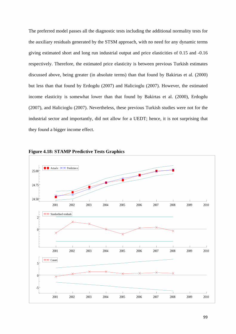
99
The preferred model passes all the diagnostic tests including the additional normality tests for
the auxiliary residuals generated by the STSM approach, with no need for any dynamic terms
giving estimated short and long run industrial output and price elasticities of 0.15 and -0.16
respectively. Therefore, the estimated price elasticity is between previous Turkish estimates
discussed above, being greater (in absolute terms) than that found by Bakirtas et al. (2000)
but less than that found by Erdogdu (2007) and Halicioglu (2007). However, the estimated
income elasticity is somewhat lower than that found by Bakirtas et al. (2000), Erdogdu
(2007), and Halicioglu (2007). Nevertheless, these previous Turkish studies were not for the
industrial sector and importantly, did not allow for a UEDT; hence, it is not surprising that
they found a bigger income effect.
Figure 4.18: STAMP Predictive Tests Graphics
2001 2002 2003 2004 2005 2006 2007 2008 2009 201024.50
24.75
25.00Actual e Prediction e
2001 2002 2003 2004 2005 2006 2007 2008 2009 2010
0
2Standardised residuals
2001 2002 2003 2004 2005 2006 2007 2008 2009 2010
-5
0
5Cusum

100
Table 4.3: Turkish Industrial Electricity Demand STSM Estimates and Diagnostics Sample 1960-2008 Variables Estimated
Coefficients Standard Errors
Probabilities
p -0.16086 0.04483 0.001
y 0.14969 0.05142 0.007
Lvl 1979 -0.16873 0.03436 0.000
Slp 1981 -0.03883 0.01378 0.007
Irr 1991 -0.08426 0.02793 0.006
Level and Slope Components of UEDT2008
Level 22.06831 Slope 0.08677
Residuals
Auxiliary Residuals
Irregular Level Slope
Std. Error 0.923 Std. Error 1.011 0.992 0.911 Normality 0.466 Normality 0.689 0.634 0.278 Skewness 0.382 Skewness 0.617 0.438 0.112 Kurtosis 0.382 Kurtosis 0.482 0.661 0.872 H(14) 0.594
- - -
R(1) 0.023
- - - R(7) 0.146
- - -
DW 1.945
- - - Q(7,5) 4.244
- - -
Predictive Test 2001-2008
LR Test
Failure 0.9048
Test (a) 96.31 (0.000) Cusum t(4) 0.7996
Test (b) 22.72 (0.000)
Goodness of Fit
Hyperparameters
p.e.v. 0.001
Level 0.0003149 p.e.v./m.d.2 1.137
Slope 0.0001536
R2 0.999
Irregular 0.0004675 Rd
2 0.651
Nature Of Trend :
Local Trend Model
Notes: -Model estimation and all statistics are from STAMP 8.10;
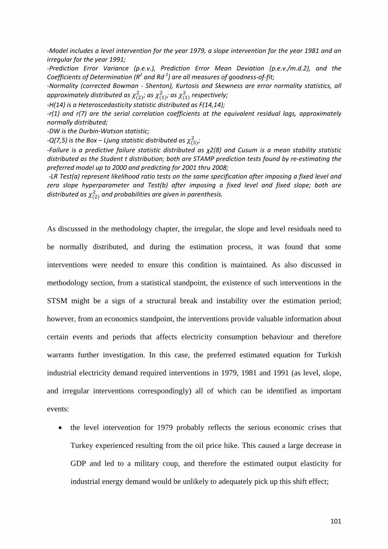
101
-Model includes a level intervention for the year 1979, a slope intervention for the year 1981 and an irregular for the year 1991; -Prediction Error Variance (p.e.v.), Prediction Error Mean Deviation (p.e.v./m.d.2), and the Coefficients of Determination (R2 and Rd 2) are all measures of goodness-of-fit; -Normality (corrected Bowman - Shenton), Kurtosis and Skewness are error normality statistics, all approximately distributed as 𝜒(2)
2 ; as 𝜒(1)2 ; as 𝜒(1)
2 respectively; -H(14) is a Heteroscedasticity statistic distributed as F(14,14); -r(1) and r(7) are the serial correlation coefficients at the equivalent residual lags, approximately normally distributed; -DW is the Durbin-Watson statistic; -Q(7,5) is the Box – Ljung statistic distributed as 𝜒(5)
2 ; -Failure is a predictive failure statistic distributed as χ2(8) and Cusum is a mean stability statistic distributed as the Student t distribution; both are STAMP prediction tests found by re-estimating the preferred model up to 2000 and predicting for 2001 thru 2008; -LR Test(a) represent likelihood ratio tests on the same specification after imposing a fixed level and zero slope hyperparameter and Test(b) after imposing a fixed level and fixed slope; both are distributed as 𝜒(2)
2 and probabilities are given in parenthesis.
As discussed in the methodology chapter, the irregular, the slope and level residuals need to
be normally distributed, and during the estimation process, it was found that some
interventions were needed to ensure this condition is maintained. As also discussed in
methodology section, from a statistical standpoint, the existence of such interventions in the
STSM might be a sign of a structural break and instability over the estimation period;
however, from an economics standpoint, the interventions provide valuable information about
certain events and periods that affects electricity consumption behaviour and therefore
warrants further investigation. In this case, the preferred estimated equation for Turkish
industrial electricity demand required interventions in 1979, 1981 and 1991 (as level, slope,
and irregular interventions correspondingly) all of which can be identified as important
events:
• the level intervention for 1979 probably reflects the serious economic crises that
Turkey experienced resulting from the oil price hike. This caused a large decrease in
GDP and led to a military coup, and therefore the estimated output elasticity for
industrial energy demand would be unlikely to adequately pick up this shift effect;

102
• the slope intervention for 1981 probably reflects the important change in Turkish
industrial electricity consumption, because of the first implementation of planned
energy conservation activities for the industrial sector by the General Directorate of
Electrical Power Resources Survey Administration-EIE (Hepbasli and Ozalp, 2003);
• the irregular intervention for 1991 probably reflects the economic crisis that year
following from the Gulf war and sanctions against Iraq; the export oriented Turkish
industrial sector was quite negatively affected bringing about a 4% reduction in
industrial electricity consumption, which would not be captured adequately by the
estimated output and price elasticities (being outside the usual ‘norm’).
It would appear that the 1991 and 1979 crises effected Turkish industry in a different manner.
As discussed in the introduction, prior to the 1980s the Turkish economy was inward looking
with an import-substituting industrialization strategy; whereas, after 1980 the strategy
changed with an export oriented industrialization strategy adopted. Therefore, before 1980
the domestic market is more important whereas after 1980 exports became more important.
Even though Turkey experienced a bigger domestic economic crisis in 2001 compared to
1991, the 1991 crises had a narrowing effect on export potential of Turkey because of the
first gulf war.
The estimated UEDT from this procedure is non-linear given the estimated hyper-parameters
(Table 4.3) and is illustrated in Figure 4.19. It can be seen that the estimated stochastic trend
is generally increasing (but at a decreasing rate) over the estimation period, i.e. it is generally
energy using. It also clear in Figure 4.20, given the interventions, that there is a level drop in
1979 and the slope changes at 1981; moreover Figure 4.20 illustrates that the slope and the

103
‘adjusted slope’ generally diminishes over the estimation period.33 The preferred equation
and the estimated non-linear UEDT are now used to construct future scenarios for Turkish
energy demand, which are explained in the next section.
Figure 4.19: Underlying Electricity Demand Trend (UEDT) of Turkish Industrial Sector Electricity Consumption 1960-2008
Figure 4.20: Slope and Level of UEDT for Turkish Industrial Sector 1960-2008
33 The estimated ‘adjusted slope’ is equal to the estimated slope plus the slope intervention.
1960 1965 1970 1975 1980 1985 1990 1995 2000 2005 2010
17.5
18.0
18.5
19.0
19.5
20.0
20.5
lnUEDT for Turkish Industrial Electricity Consumption
1960 1965 1970 1975 1980 1985 1990 1995 2000 2005 2010
18
19
20
21
22
lnLevel Adjusted Level (=UEDT) with Slope, Level and Irregular Interventions
1960 1965 1970 1975 1980 1985 1990 1995 2000 2005 2010
0.04
0.06
0.08
0.10
ln
Slope Adjusted Slope with Slope Intervention

104
4.9.2 Turkish Residential Electricity Demand
After eliminating the insignificant variables and including interventions in order to maintain
the normality of residuals and auxiliary residuals, a summary of the preferred estimated
equation for Turkish residential demand is given by:
𝑒𝑡 = 0.75767𝑒𝑡−1 + 0.37978𝑦𝑡−1 − 0.09171𝑝𝑡 + 𝑈𝐸𝐷𝑇𝑡 (4.3)
where 𝑈𝐸𝐷𝑇2008 = -4.43093 at the end of the period. The detailed estimation results and the
diagnostics tests are given in Table 4.4. The model passes all the diagnostic tests including
the additional normality tests for the auxiliary residuals generated by the STSM approach.
This includes the STAMP prediction tests over 2001 – 2008, as illustrated in Figure 4.21.
The previous years’ electricity consumption has a significant effect on residential sector
electricity consumption the magnitude being just above 75%. In the short run, household
appliances are fixed and given the derived demand nature of residential electricity, the short
run impact of changes in prices and income is limited. However, in the long run households
are able to change the appliances so that the household expenditure and price elasticities will
be greater in the long run.
The estimated results suggest that expenditure does not have a significant impact in the
current year; that is the ‘impact elasticity’ is estimated to be zero. However, the impact of
expenditure is estimated to come through during the next year; hence, this is interpreted here
as the ‘short run’ expenditure elasticity of 0.38. This compares to the estimated ‘impact/short
run’ price elasticity of -0.09. Whereas the estimated long run residential expenditure and
price elasticities are 1.57 and -0.38 respectively.

105
Table 4.4: Turkish Domestic Electricity Demand STSM Estimates and Diagnostics Sample 1960-2008 Variables Estimated
Coefficients Standard Errors
Probabilities
et-1 0.75767 0.05054 0.000
yt-1 0.37978 0.08089 0.000
pt -0.9171 0.04432 0.045 Irr 1973 -0.1345 0.03008 0.000
Level 1971 -0.1199 0.03688 0.002
Level 1975 0.1013 0.03931 0.014
Components Of UEDT2008
Long Run Elasticity Estimates
Level -4.4124
Price -0.38 Slope -
Income 1.57
Auxiliary Residuals
Residuals
Irregular Level Slope Std. Error 0.960 Std. Error 0.986 0.969 - Normality 0.281 Normality 0.816 0.299 - Skewness 0.111 Skewness 0.827 0.120 - Kurtosis 0.967 Kurtosis 0.549 0.992 - H(13) 1.201
- - -
R(1) 0.047
- - - R(6) 0.099
- - -
DW 1.856
- - - Q(6,5) 1.563
- - -
Predictive Test 2001-2008
LR Test
Failure 0.30
Test (a) 30.507 (0.0000) Cusum t(4) 0.97
Test (b) 19.954 (0.0000)
Goodness of Fit
Hyperparameters
p.e.v. 0.001
Level 0.00111 p.e.v./m.d.2 1.134
Slope -
R2 0.999
Irregular 0.00044 Rd
2 0.720
Nature of Trend:
Local Level Model

106
Notes: -See notes to Table 4.334 -Model includes a level intervention for the year 1971, an irregular for the year 1973 and a level intervention for the year 1975; -LR Test(a) represent likelihood ratio tests on the same specification after imposing a fixed level and zero slope hyperparameter and Test(b) after imposing a fixed level and fixed slope; both are distributed as 𝜒(2)
2 and probabilities are given in parenthesis.
Figure 4.21: STAMP Prediction Test Graphics
The estimated UEDT is the local level model that consists of a stochastic level but no slope
and is shown in Figure 4.22, which illustrates that the estimated UEDT decreases and
increases over the estimation period. This UEDT would appear to reflect the compulsory
electricity cuts introduced by the Turkish governments (primarily in the residential sector)
aimed at conserving electricity consumption between 1971 and 1983. An irregular
intervention in 1973 and level interventions in 1971 and 1975 were required in order to
maintain the normality of residuals and auxiliary residuals. The level interventions appear to
34For simplicity and to save space the notes given in the previous table are not repeated again.
2001 2002 2003 2004 2005 2006 2007 2008 2009 2010
23.8
24.0
24.2
24.4Actual e Prediction e
2001 2002 2003 2004 2005 2006 2007 2008 2009 2010
-5
0
5Cusum

107
reflect the impact of cuts on the behaviours of consumers in 197135 that were almost reversed
in 1975 (probably reflecting the way consumers adjusted their behaviour accordingly).
Figure 4.22: Underlying Electricity Demand Trend of Turkish Residential Sector 1961-2008
The irregular intervention for the year 1973 probably reflects the impact of the electricity cuts
that peaked in 1973 by a factor of 37 from 1972 to 1973 and kept increasing slightly after
1973 (Altas et al. 1994) as illustrated in Figure 4.23. Thus in 1973 it appears that desired
residential demand was severely constrained by the cuts; hence the need for the irregular
intervention. Moreover, given the intervention for 1973 represents a ‘pulse effect’ it does not
affect the electricity consumption permanently, only in 1973 electricity consumption decrease
14% for the year.
35 The electricity cuts that were applied for couple of hours during the day decrease the level of total electricity consumption permanently by 12%.
1960 1965 1970 1975 1980 1985 1990 1995 2000 2005 2010
-4.75
-4.70
-4.65
-4.60
-4.55
-4.50
-4.45
-4.40UEDT for Turkish Residential Electricty
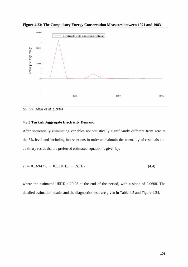
108
Figure 4.23: The Compulsory Energy Conservation Measures between 1971 and 1983
Source: Altas et al. (1994)
4.9.3 Turkish Aggregate Electricity Demand
After sequentially eliminating variables not statistically significantly different from zero at
the 5% level and including interventions in order to maintain the normality of residuals and
auxiliary residuals, the preferred estimated equation is given by:
𝑒𝑡 = 0.16947𝑦𝑡 − 0.11101𝑝𝑡 + 𝑈𝐸𝐷𝑇𝑡 (4.4)
where the estimated UEDTtis 20.95 at the end of the period, with a slope of 0.0608. The
detailed estimation results and the diagnostics tests are given in Table 4.5 and Figure 4.24.
1975 1980 1985
0
1500
3000
4500An
nual
perce
ntage
chan
ge
Electricity cuts and conservations

109
Table 4.5: Turkish Total Electricity Demand STSM Estimates and Diagnostics Sample 1960-2008
Variables Estimated Coefficients
Standard Errors
Prob.
yt 0.16947 0.06162 0.001 pt -0.11101 0.02384 0.001 Level Break 1976 0.09233 0.03696 0.004 Level Break 1979 -0.08495 0.06162 0.009 Level And Slope Components’ of UEDT2008 Level : 20.9526 Slope : 0.0608 Diagnostics Residuals Auxiliary Residuals Irregular Level Slope Std.Error 0.918 Std.Error 0.999 0.974 0.883 Normality 0.895 Normality 0.702 0.629 0.394 Skewness 0.734 Skewness 0.456 0.602 0.694 Kurtosis 0.744 Kurtosis 0.696 0.418 0.191 H(14) 0.675 r(1) -0.002 r(7) 0.006 DW 1.908 Q(7,5) 4.806 Hyperparameters Goodness of fit Level 0.00004 p.e.v. 0.001 Slope 0.00003 p.e.v./md2 1.120 R2 0.999 Rd
2 0.655 Predictive Tests 2001-2008 LR TEST Failure 0.92 Test(a) 72.992 0.000 Cusum t(4) 0.99 Test(b) 17.336 0.000 Nature Of Trend: Local Level Notes: -See notes to Table 4.336 -Model includes level interventions for 1976 and 1979;
36For simplicity and to save space the full notes already given in Table 4.3 are not repeated.
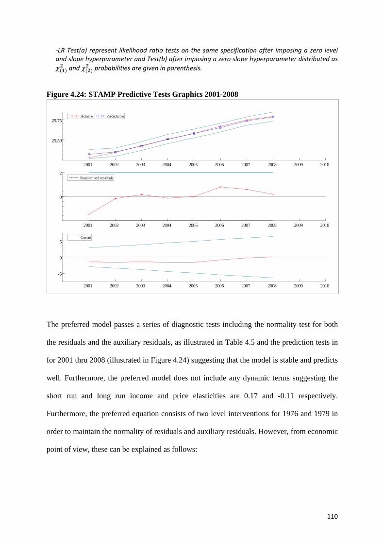
110
-LR Test(a) represent likelihood ratio tests on the same specification after imposing a zero level and slope hyperparameter and Test(b) after imposing a zero slope hyperparameter distributed as 𝜒(1)
2 and 𝜒(2)2 probabilities are given in parenthesis.
Figure 4.24: STAMP Predictive Tests Graphics 2001-2008
The preferred model passes a series of diagnostic tests including the normality test for both
the residuals and the auxiliary residuals, as illustrated in Table 4.5 and the prediction tests in
for 2001 thru 2008 (illustrated in Figure 4.24) suggesting that the model is stable and predicts
well. Furthermore, the preferred model does not include any dynamic terms suggesting the
short run and long run income and price elasticities are 0.17 and -0.11 respectively.
Furthermore, the preferred equation consists of two level interventions for 1976 and 1979 in
order to maintain the normality of residuals and auxiliary residuals. However, from economic
point of view, these can be explained as follows:
2001 2002 2003 2004 2005 2006 2007 2008 2009 2010
25.50
25.75Actual e Prediction e
2001 2002 2003 2004 2005 2006 2007 2008 2009 2010
0
2Standardised residuals
2001 2002 2003 2004 2005 2006 2007 2008 2009 2010
-5
0
5Cusum

111
• the level intervention for 1976 probably reflects the unusual 9% increase in Turkish
GDP and 12% decrease in real average Turkish electricity prices in 1976. The
coincidence of both of these unusual circumstances brought about an increase of 20%
in aggregate electricity consumption which would not be captured by the estimated
income and price elasticities (being outside the usual ‘norm’);
• the level intervention for 1979 probably reflects the serious economic crisis that
Turkey experienced resulting from the world oil price hike. This caused a large
decrease in GDP and led to a military coup, and therefore the estimated elasticities for
total electricity demand would be unlikely to adequately pick up this effect;
The estimated UEDT from this procedure is given by the estimated hyperparameters (Table
4.5) and is illustrated in Figure 4.25 and Figure 4.26. It can be seen that the estimated
stochastic trend is increasing with a break in 1976 and 1979 over the estimation period.
Figure 4.25: Underlying Electricity Demand Trend of Turkey 1960-2006
1960 1965 1970 1975 1980 1985 1990 1995 2000 2005 2010
17.5
18.0
18.5
19.0
19.5
20.0
20.5
21.0UEDT for Turkish Total Electricity Demand

112
Figure 4.26: Slope of UEDT for Turkish Total Electricity 1960-2008
Given the preferred equations for industrial, residential, and aggregate electricity demand
with the estimated UEDTs has been uncovered; they are now used to construct future
scenarios for Turkish electricity demand, which is explained in the next section.
4.10 Forecast Scenarios and Assumptions
As described in the methodology section three scenarios are implemented namely reference,
high case, and low case. Although, where data (and ‘intelligence’) are available for 2009
(such as the nominal industrial electricity price) 37 these are used in all scenarios. This
therefore produces the forecast scenarios up to 2020 for aggregate, residential and industrial
electricity demand based upon the estimated equations discussed in the previous section as 37In 2009, Turkish industrial electricity prices increased by 18% in nominal terms. At the time of writing, the required deflator (the Consumer Price Index from World Bank) is not available, although it is known that Turkish inflation was around 6.5% in 2009; hence based on this the real industrial electricity price is assumed to have increased by 11.5% in 2009 for all three scenarios. In 2009 the average price of electricity (weighted average of residential and industrial prices) prices increased by 18.5% in nominal terms. Hence, based on this, average electricity price is assumed to have increased by 12% in 2009 for all three scenarios. In 2009 Turkish residential electricity prices increase d by 19.3 % in nominal terms; hence, based on this, the real residential electricity price is assumed to have increased by 12.8% in 2009 for all three scenarios.
1960 1965 1970 1975 1980 1985 1990 1995 2000 2005 2010
0.06
0.07
0.08
0.09
0.10
0.11 Slope of UEDT for Turkish Total Electricity

113
well as the ‘residual’ sector as described in the methodology chapter. The detailed
information about the scenario assumptions follows.
• In the ‘reference’ scenario, it is assumed that real industrial, residential, and average
electricity prices will increase 1% after 2009 annually (Figure 4.27). The Turkish
Parliament ratified the Kyoto protocol and it is likely that the government will
introduce measures such as carbon taxes and incentives to encourage renewables,
which are likely to contribute to an increase in end use prices of electricity. However,
the improving efficiency in electricity generation is likely to reduce the cost and
hence, counteract the price increase to some extent. Consequently, it is assumed that
real industrial, residential, and average electricity prices will increase 1% annually.
Figure 4.27: Reference Scenario for Residential, Industrial, and Aggregate Electricity Prices 2000-2020
2000 2005 2010 2015 2020
0.075
0.150
0.225
0.300
0.375
2005
con
stan
t YTL
Residential Electricity Prices Aggregate Electricity Prices
Industrial Electricity Pirces

114
The increase of industrial value added (output) is expected to be 1.5% in 2009, and
2% for 2010 and 2012 because of the global crises. It is further assumed that there
would then follow a recovery period with annual increases of 2.5%, 3% and 3.5% for
2013 to 2015 and a 4% per annum thereafter (Figure 4.28). The increase of total
household final consumption expenditure (expenditure) is assumed to be 1% in 2009
because of the global crises followed by a recovery period with an annual expenditure
increasing by 2% per year in 2010 thru 2012, 3% per year in 2013 thru 2016 and 3.5%
per year thereafter (Figure 4.28).The increase of GDP is assumed to be 1% in 2009
due to the global economic slowdown, followed by a recovery period with GDP
increasing by 1.5% per annum in 2010 thru 2012, 2% per annum in 2013 thru 2016
and 2.5% per annum thereafter (Figure 4.28).
Figure 4.28: Reference Scenario for Expenditure, Output, and GDP 2000-2020
2000 2005 2010 2015 2020
200
400
600
800
1000
2005
con
stan
t bill
ion
YTL
Expenditure GDP
Output

115
Given that the adjusted slope of the UEDT generally diminishes over the estimation
period for industrial electricity demand, it is assumed that this will continue into the
future, hence it is assumed that the adjusted slope decreases by 0.0011 each year from
the estimated value of 0.04793 in the last period of the estimation (Figure 4.29).38 It
implicitly assumes that the annual change in exogenous ‘energy using’ behaviour for
Turkish industrial electricity demand at the end of the estimation period will continue
to increase but at a decreasing rate throughout the forecast period. The residential
electricity demand is a local level model with no estimated slope, this suggests that
the UEDT for residential electricity demand is fixed over the future at the estimated
level in 2008. However, given that the estimated UEDT generally rises its average
change over the estimation period is utilized for the slope of the UEDT after 2008; it
is therefore assumed that the slope of the UEDT is 0.003 for the ‘reference’ scenario
(Figure 4.29).39 This assumption suggests that the general electricity using behaviour
of the Turkish residential sector by the estimated UEDT will continue into the future.
Additionally, for aggregate electricity demand it is assumed that the observed
generally diminishing slope of the UEDT over the estimation period continues to
decrease by 0.00140 each year (Figure 4.29).
• In the ‘low’ case scenario, it is assumed that the reduction in the costs of power
production due to increased efficiency in electricity generation are relatively small;
hence these savings are outweighed by the rise in prices brought about from the
38The figure of -0.0011 being the average change in the estimated adjusted slope over the estimation period.
39As opposed to the zero suggested by the estimation results.
40 The figure -0.001 is therefore the average change in the estimated slope over the estimation period.

116
measures introduced in order to comply with the Kyoto Protocol. The assumed rise in
real electricity prices is therefore 2% per annum after 2009 (Figure 4.30).
Figure 4.29: Reference Scenario for Residential, Industrial, and Aggregate UEDTs 2000-2020
For industrial value added it is assumed that it will decrease 3% in 2009 and increase
0.5% in 2010 and 2011 because of the global economic crises and increase by 1% in
2012, 1.5% in 2013, 1.5% in 2014, 2% per year in 2015 and 2016 and 2.5% thereafter
until 2020 (Figure 4.31). The annual increase of total household final expenditure is
assumed to decrease 0.5% in 2009, increase 1.5% per year in 2010 thru 2012 because
of the global economic crises, but then increase 2% per year in 2013 thru 2016, and
2.5% per year thereafter (Figure 4.31). GDP is assumed to increase by only 0.5% in
2009 due to the global economic crisis and by only 1% per annum in 2010 thru 2012
2000 2005 2010 2015 2020
-4.60-4.55-4.50-4.45-4.40-4.35 UEDT for Residential Electricity
2000 2005 2010 2015 2020
19.019.520.020.521.021.522.022.5
UEDT for Industrial Electricity
2000 2005 2010 2015 2020
19.019.520.020.521.021.522.022.5
UEDT for Aggregate Electricity
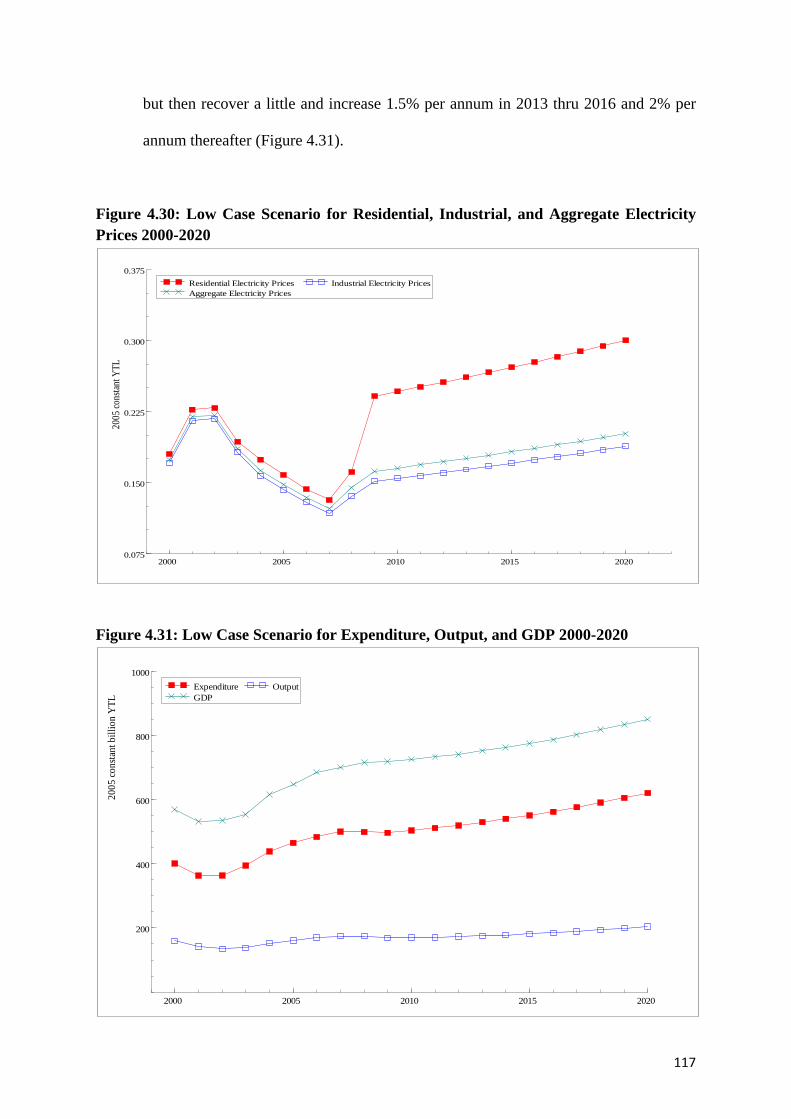
117
but then recover a little and increase 1.5% per annum in 2013 thru 2016 and 2% per
annum thereafter (Figure 4.31).
Figure 4.30: Low Case Scenario for Residential, Industrial, and Aggregate Electricity Prices 2000-2020
Figure 4.31: Low Case Scenario for Expenditure, Output, and GDP 2000-2020
2000 2005 2010 2015 20200.075
0.150
0.225
0.300
0.375
2005
cons
tant Y
TL
Residential Electricity Prices Aggregate Electricity Prices
Industrial Electricity Prices
2000 2005 2010 2015 2020
200
400
600
800
1000
2005
cons
tant b
illio
n YT
L
Expenditure GDP
Output

118
Because of improved efficiency and faster transformation of the Turkish industrial
sector, it is assumed that the adjusted slope of the UEDT decreases by 0.0033 each
year (Figure 4.32).41 It is thus assumed that the exogenous underlying ‘energy using’
behaviour for Turkish industrial electricity demand will continue throughout the
forecast period, but is offset by some improvement in efficiency. Furthermore, for the
UEDT a shock effect is included for 2009 with the same magnitude as that estimated
by the irregular intervention for 1991 in order to take into account a shock that might
have occurred because of the global crisis. In the ‘low’ case scenario, an energy using
UEDT for residential electricity demand with a decreasing slope of 0.001 is
introduced from 2009 (Figure 4.32). This assumption express the view that energy
using UEDT will continue but at a slower pace than the ‘reference’ scenario because
of an increase in energy efficiency. Furthermore, for aggregate electricity demand, it
is assumed that the slope of the UEDT decreases by 0.003 per annum, suggesting that
the ‘energy using’ trend for electricity will continue, but at a slower pace (Figure
4.32).
41 The figure of -0.0033 is obtained by assuming that over the forecast period the adjusted slope declines by an additional factor of two of the average change over the estimation period.

119
Figure 4.32: Low Case Scenario for Residential, Industrial, and Aggregate UEDTs 2000-2020
• In the ‘high’ case scenario, the real electricity prices is assumed to increase 0.5% per
year over the period 2010 to 2020 period (Figure 4.33). Even though the Kyoto
protocol is ratified by the Turkish parliament, and is likely to result in new carbon
taxes, in this scenario it is assumed that the increasing efficiency standards in
electricity generation will decrease the cost of power production. Therefore, it is
assumed that these two factors balance each other out and the electricity price will
increase only 0.5% per year in real terms.
2000 2005 2010 2015 2020
-4.60-4.55-4.50-4.45-4.40-4.35 UEDT for Residential Electricity
2000 2005 2010 2015 2020
19.019.520.020.521.021.522.022.5
UEDT for Industrial Electricity
2000 2005 2010 2015 2020
19.019.520.020.521.021.522.022.5
UEDT for Aggregate Electricity

120
Figure 4.33: High Case Scenario for Residential, Industrial, and Aggregate Prices 2000-2020
Furthermore, it is assumed that industrial value added will increase by 3% each year
in 2009 and 2010 and 2.5% in 2011, because of the global economic crisis. It is
further assumed that this is followed by a recovery period with an increase of 3% in
2012, 3.5% per year in 2013 4.5% per year in 2014 and 2015, 5% per year in 2016
and 2017 and slightly higher at 6% per year thereafter (Figure 4.34). Moreover, it is
assumed that total household total final consumption expenditure will increase by
1.5% in 2009 and 2.5% per year in 2010 thru 2012, followed by a 3.5% per year
increase in 2013 thru 2016. It is further assumed that the annual increase of
expenditure will be 4% per year thereafter (Figure 4.34). In addition, it is assumed
that GDP will still see an increase of 1.5% in 2009 despite the global slowdown,
followed by a good recovery increasing by 2% per annum in 2010 thru 2012,
2000 2005 2010 2015 2020
0.075
0.150
0.225
0.300
0.375
2005
con
stan
t YTL
Residential Electricity Prices Aggregate Electricity Prices
Industrial Electricity Prices

121
followed by 2.5% per annum in 2013 thru 2016, and 3% per annum thereafter to 2020
(Figure 4.34).
Figure 4.34: High Case Scenario for GDP, Output, and Expenditure 2000-2020
For the UEDT of industrial electricity demand, it is assumed that the slope will
increase by 0.0011 each year (Figure 4.35);42 implicitly assuming that the exogenous
‘energy using’ behaviour for industrial electricity demand increases at an even greater
pace. Additionally, for residential sector contrary to the ‘low’ case scenario, an energy
using UEDT is assumed with a slope of 0.007 from 2009 (Figure 4.35), assuming that
the exogenous ‘energy using’ behaviour for the residential electricity demand
increases at an even greater pace. Finally, for the aggregate electricity demand it is
assumed that the slope of the UEDT will increase 0.001 per annum from 2009 to 2020
42The figure of +0.0011 mirrors that assumed for the ‘low’ scenario.
2000 2005 2010 2015 2020
200
400
600
800
1000
2005
con
stan
t bill
ion
YTL
Expenditure GDP
Output

122
(Figure 4.35), suggesting that the ‘energy using’ trend for electricity will continue, but
at a faster pace.
Figure 4.35: High Case Scenario for Residential, Industrial, and Aggregate UEDTs 2000-2020
In order to summarise together the above assumptions for the ‘reference’, ‘low’, and ‘high’
case for each variables are given in Figure 4.36.
2000 2005 2010 2015 2020
-4.60-4.55-4.50-4.45-4.40-4.35 UEDT for Residential Electricity
2000 2005 2010 2015 2020
19.019.520.020.521.021.522.022.5
UEDT for Industrial Electricity
2000 2005 2010 2015 2020
19.019.520.020.521.021.522.022.5
UEDT for Aggregate Electricity

123
Figure 4.36: Scenario Assumptions A: Reference, Low, and High Case Scenarios for Residential, Industrial, and Aggregate Electricity Prices
B: Reference, Low, and High Case Scenarios for Expenditure, Output, and GDP
2000 2005 2010 2015 2020
0.15
0.20
0.25
0.30
0.35
2005
con
stan
t YTL Residential Electricity Prices
Residential Electricity Prices (Low) Residential Electricity Prices (Ref) Residential Electricity Prices (High)
2000 2005 2010 2015 2020
0.15
0.20
0.25
2005
con
stan
t YTL
2005
con
stan
t YTL
Industrial Electricity Prices Industrial Electricity Prices (Low)
Industrial Electricity Pirces (Ref) Industrial Electricity Prices (High)
2000 2005 2010 2015 2020
0.15
0.20
Aggregate Electricity Prices Aggregate Electricity Prices (Low)
Aggregate Electricity Prices (Ref) Aggregate Electricity Prices (High)
2000 2005 2010 2015 2020
500
700
2005
con
stant
bill
ion
YTL
Expenditure Expenditure (Low)
Expenditure (Ref) Expenditure (High)
2000 2005 2010 2015 2020
150
200
250
300
2005
con
stant
bill
ion
YTL
Output Output (Low)
Output (Ref) Output (High)
2000 2005 2010 2015 2020
600
800
2005
con
stant
bill
ion
YTL
GDP GDP (Low)
GDP (Ref) GDP (High)

124
C: Reference, Low, and High Case Scenarios for Residential, Industrial, and Aggregate Electricity UEDTs
4.11 Forecast Results:
4.11.1 Turkish Industrial Electricity Demand
Based on the estimated equation presented in the previous section and applying the scenario
assumptions discussed above, Turkish industrial electricity demand is predicted to be 97, 121,
and 148 TWh by 2020 according to the ‘low’, ‘reference’ and ‘high’ case scenarios
respectively. The paths to 2020 for the three scenarios are illustrated in Figure 4.37.
2000 2005 2010 2015 2020
-4.45
-4.40
-4.35UEDT for Residential Electricity UEDT for Residential Electricity (Low)
UEDT for Residential Electricity (Ref) UEDT for Residential Electricity (High)
2000 2005 2010 2015 2020
20.5
21.0
21.5UEDT for Industrial Electricity UEDT for Industrial Electricity (Low)
UEDT for Industrial Electricity (Ref) UEDT for Industrial Electricity (High)
2000 2005 2010 2015 202020.5
21.0
21.5UEDT for Aggregate Electricity UEDT for Aggregate Electricity (Low)
UEDT for Aggregate Electricity (Ref) UEDT for Aggregate Electricity (High)

125
Figure 4.37: Turkey’s Industrial Electricity Demand Forecast over the period 2009-2020
4.11.2 Turkish Residential Electricity Demand
Given the above assumptions, it is predicted that future residential electricity consumption in
2020 will be 48 TWh, 64 TWh and 80 TWh in the, ‘low’, ‘reference’ and ‘high’ case
scenarios respectively. The annual residential electricity consumption forecast scenarios over
the period 2009-2020 are given in Figure 4.38.
2000 2005 2010 2015 2020
40
50
60
70
80
90
100
110
120
130
140
150TWh
Industrial_Electricity_Consumption Low
Reference High

126
Figure 4.38: Turkey’s Residential Electricity Demand Forecast over the period 2009-2020
4.11.3 Turkish Aggregate Electricity Demand
Given the above assumptions, future Turkish aggregate electricity consumption is predicted
to be 259, 310, and 368 TWh in the ‘low’, ‘reference’ and ‘high’ case scenarios respectively
as illustrated in Figure 4.39.
2000 2005 2010 2015 2020
30
40
50
60
70
80TWh
Residential_Electricity_Consumption Low_Case
Refference High_Case
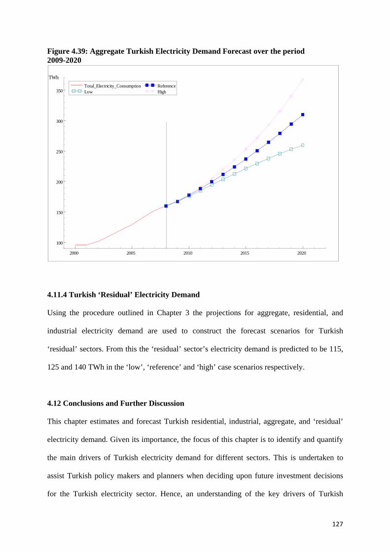
127
Figure 4.39: Aggregate Turkish Electricity Demand Forecast over the period 2009-2020
4.11.4 Turkish ‘Residual’ Electricity Demand
Using the procedure outlined in Chapter 3 the projections for aggregate, residential, and
industrial electricity demand are used to construct the forecast scenarios for Turkish
‘residual’ sectors. From this the ‘residual’ sector’s electricity demand is predicted to be 115,
125 and 140 TWh in the ‘low’, ‘reference’ and ‘high’ case scenarios respectively.
4.12 Conclusions and Further Discussion
This chapter estimates and forecast Turkish residential, industrial, aggregate, and ‘residual’
electricity demand. Given its importance, the focus of this chapter is to identify and quantify
the main drivers of Turkish electricity demand for different sectors. This is undertaken to
assist Turkish policy makers and planners when deciding upon future investment decisions
for the Turkish electricity sector. Hence, an understanding of the key drivers of Turkish
2000 2005 2010 2015 2020
100
150
200
250
300
350
TWhTotal_Electricity_Consumption Low
Reference High

128
electricity demand and their impact are vital for policy implementation and evaluation.
Therefore, given the results here not only should the estimated price and income elasticities
be incorporated in any policy analysis but also the estimated UEDT to hopefully avoid some
of the mistakes made in the past.
Ediger and Tatlidil (2002), Keleş (2005), Ediger and Akar (2007), Hamzacebi (2007), Akay
and Atak (2006) argue that previous electricity demand forecasts for Turkey were mostly
unsuccessful. A possible reason for this might be that the UEDT, structural changes and
breaks in energy demand behaviour, and the impact of previous shocks were not adequately
taken into account in the models underpinning the forecasts, and arguably, they should be in
order to make useful and usable forecasts. Since the STSM enables the UEDT to be estimated
it provides valuable information about the structural change and breaks in electricity
consumption behaviour and adjustment process related to shocks to the system. It is therefore
concluded that the STSM approach is the right solution for determining forecasts of future
energy demand.
As stated above this chapter estimates the Turkish residential, industrial, aggregate and
‘residual’ electricity demand functions by using STSM approach which was not done before,
as far as known. Therefore, the findings of this chapter can be summarized as follows:
For residential electricity demand: it is found that the estimated household total final
expenditure elasticity is 0.38 in the short run and 1.57 in long run. Additionally the short run
and long run price elasticity is -0.09 and -0.38 respectively. Furthermore, this chapter has
uncovered the UEDT for the Turkish residential sector, which is highly stochastic with
increasing and decreasing periods.

129
The trend in Turkish residential electricity consumption was generally diminishing between
1971 and 1983 (except for 1974, 1975, 1976, and 1981) and, as discussed above, probably
reflects the compulsory conservation measurements (in addition to the impact in 1973
identified by the irregular intervention) that were adopted by the government between 1971
and 1983 and identified by the STSM. This arguably illustrates the power of this approach in
distinguishing the structural changes of demand behaviour. In addition, after the end of these
compulsory conservation measurements starting from 1982, the UEDT follows a generally
increasing trend until 1996 and follows a stochastic movement afterwards until the end of
estimation period.
The only previous study focusing on estimating Turkish residential electricity demand
function Halicioglu (2007), found estimated short run and the long run price elasticities of
-0.33 and -0.52 respectively. Although the estimated short run price elasticity is somewhat
different to the -0.09 obtained here, the long run estimate is similar to the estimated -0.38
found here. This is probably due to firstly, the different real price variable used and secondly
the inclusion of the UEDT in this study. Arguably, the more relevant price variable and the
inclusion of the UEDT in this study render it more appropriate and therefore more reliable.
Additionally, Halicioglu (2007) found the estimated short run and long run income
elasticities to be 0.44 and 0.70 respectively. Although the estimated short run expenditure
elasticity of 0.38 found here is similar to that of the income elasticity in Halicioglu (2007),
the estimated long run expenditure elasticity of 1.57 differs considerably. These differences
are probably due to first, the different activity variables used and second, as with price, the
inclusion of the UEDT in this study. It is believed that the expenditure variable used for
economic activity here is more appropriate for residential electricity demand.

130
Given the analysis undertaken, it is expected under the different forecast assumptions (Figure
4.41) that Turkish residential electricity consumption will be between 48 and 80 TWh by the
year 2020. There is only one previous forecast study Hamzacebi (2007) which predicted that
the residential electricity consumption would be 257 TWh in 2020, which is noticeably
greater than even the high case scenario of this study. This forecast is arguably highly
unlikely and unreasonable. Hamzacebi (2007) does not investigate the relation between
economic activity and residential electricity consumption but as was explained earlier, the
electricity demand highly affected by economic activity. Thus, any forecast that ignores this
effect will arguably lead to a misleading outcome.
For industrial electricity demand: it is found that industrial value added (output) elasticity is
0.15 and the estimated price elasticity is -0.16. Furthermore, the UEDT for the Turkish
industrial sector is uncovered, showing that, ceteris paribus, although electricity demand has
been increasing, the underlying rate of increase appears to be diminishing with a significant
structural change in 1981. This might well reflect the implementation of the first planned
energy conservation activities by the General Directorate of Electrical Power Resources
Survey Administration-EIE (Hepbasli and Ozalp, 2003) and illustrates once again the power
of STSM in identifying structural changes.
Because of the recent global economic crisis and the export-oriented nature of the Turkish
industrial sector a similar impact to that observed in 1991 might be observed again. Although
the Turkish economy has experienced several economic crises, it is expected that the effect of
the current global economic crisis might have an important impact on future industrial
electricity demand at least in the short to medium term; hence, it is incorporated in the ‘low’
(Figure 4.40) industrial electricity demand forecast but not the ‘reference’ and ‘high’

131
scenarios. Overall, therefore, based upon the different forecast assumptions, Turkish
industrial electricity demand is predicted to be between 90 and 106 TWh in 2015 and
between 97 and 148 TWh in 2020 (Figure 4.40). This is somewhat less than the previous
forecasts for Turkish industrial electricity demand; Akay and Atak (2006) suggested that
demand would be 140.4 TWh in 2015 and Hamzacebi (2007) suggested demand would be
219.2 TWh in 2020 – both of which are somewhat higher than the high case scenario of this
study. The difference in forecasts, it is argued, being primarily due to these other studies
neglecting the relationship between economic variables, underlying trend, and electricity
consumption.43
As far as known, there are no other previous studies that investigate the output elasticity and
industrial electricity price elasticity. Therefore, this chapter fills a gap in the literature in
terms of identifying the relationship between the economic activity, industrial electricity
prices, and industrial electricity consumption for Turkey.
For aggregate electricity demand: it is found that the estimated income and price elasticities
are 0.17 and -0.11 respectively. Furthermore, the UEDT for the aggregate electricity
consumption is estimated and is found to be generally upward sloping (energy using) but at a
generally decreasing rate. The estimated income elasticity being somewhat smaller than those
obtained by Bakırtas et al. (2000) and Erdogdu (2007) which are 3.13 and 0.41 respectively.
One of the reasons for this might be that previous studies do not take into account UEDT. As
the UEDT for Turkish aggregate electricity demand is upward sloping and the GDP generally
has been increasing over the forecast period. Therefore not taking into account UEDT might
lead over estimated income elasticity. On the other hand the estimated price elasticity is being
43 Although also probably reflects the impact of the recession in the late 2000s.

132
smaller than (in absolute terms) than that obtained by Erdoğdu (2007). This might be again
because of ignoring the UEDT coupled with the prices that have generally been declining
(although there were some price hikes in mid 1980s and 2008) over the estimation period.
These estimates are used to project future Turkish aggregate electricity. From this, it is
expected that Turkish aggregate electricity consumption will be between 259 and 368 TWh in
2020 (Figure 4.40). These forecast figures being noticeably smaller than the previous
forecasts (except by Kavaklioglu et al., 2009).
For ‘residual’ electricity demand: the results suggest that the ‘residual’ sector electricity
demand will increase faster than the industrial and residential electricity demand. One
explanation being the future Turkish economy becomes more service and commercial sector
oriented. As a result, Turkish ‘residual’ sector’s electricity demand is predicted to be between
125 and 140 TWh in 2020.
The forecast results that are generated for aggregate, residential, industrial, and ‘residual’
sectors by utilizing ‘reference’, ‘low’ case, and ‘high’ case scenarios are summarised in
Figures 4.40). As stated above the forecast outcome of this chapter will hopefully assist
Turkish policy maker and planners to avoid some of the mistakes of the past, and help them
to implement sustainable and economic policy options for Turkey.
As stated above, the previous Turkish electricity demand forecasts were mostly unsuccessful
and predicted the future electricity demand more than the actual consumption. It is argued
that these ‘over forecasts’ are due mainly to the lack of investigation into the relation between
electricity consumption, economic activity, real electricity prices and a UEDT – since, as

133
explained earlier, electricity demand is a derived demand and highly affected by these
important drivers. Thus, any forecast that ignores these effects will arguably lead to a
misleading outcome that is compounded by the inability of the Turkish authorities in
establishing credible and transparent assumptions to drive the forecast. This study therefore
addresses some of the shortcomings by introducing consistent assumptions as illustrated
above.
On the other hand, the Kyoto protocol was ratified by the Turkish Parliament in February
2009, which is leading to the introduction of legally compulsory commitments for the
reduction of greenhouse gases. Although the Copenhagen Summit in 2009 and the Cancun
Summit in 2010 did not result in any legal obligations it is reasonable to assume that
eventually there will be a legally binding agreement between nations in order to reduce GHG
emissions and that this will lead to a change in Turkish energy policy; which might well
include CO2 taxes and energy efficiency regulations. If this is the case then the new
environment will require a thorough evaluation of electricity demand relationships like those
estimated here and will be an important part of the evaluation of possible new policy
measures.
To this end, sensible and reliable energy demand forecasts assist in financing and developing
the necessary measures for the sustainable economic growth of Turkey. Furthermore, one of
the most important issues of 21st century is energy security. Arguably, the policies and
strategies cannot be neither assessed nor constructed without sound demand forecasts.
Therefore, it is suggested, that the methodology and estimated equation from this research
should be taken into account when implementing future Turkish energy policies for energy
security, climate change etc.

134
Figure 4.40: Summary of Forecast Results A: ‘Low’ Case Scenario
B: ‘Reference’ Scenario
C: ‘High’ Case Scenario
0
50
100
150
200
250
300
350
400 20
00
2001
20
02
2003
20
04
2005
20
06
2007
20
08
2009
20
10
2011
20
12
2013
20
14
2015
20
16
2017
20
18
2019
20
20
Residual Electricity
Industrial Electricity
Residential Electricity
Aggregate Electricity
0
50
100
150
200
250
300
350
400
2000
20
01
2002
20
03
2004
20
05
2006
20
07
2008
20
09
2010
20
11
2012
20
13
2014
20
15
2016
20
17
2018
20
19
2020
Residual Electricity
Industrial Electricity
Residential Electricity
Aggregate Electricity
0
50
100
150
200
250
300
350
400
2000
20
01
2002
20
03
2004
20
05
2006
20
07
2008
20
09
2010
20
11
2012
20
13
2014
20
15
2016
20
17
2018
20
19
2020
Residual Electricity
Industrial Electricity
Residential Electricity
Aggregate Electricity

135
CHAPTER 5: OECD-Europe Natural Gas Demand∗
5.1 Introduction
This chapter investigates the relationship between OECD-Europe natural gas demand and its
main determinants by applying the STSM to annual data over the period 1978 to 2009. This
is, as far as known, the first study that allows for a stochastic UEDT when estimating an
OECD-Europe natural gas demand function. After estimating the OECD-Europe natural gas
demand function by the STSM it is used to highlight the relative importance of the different
drivers and to produce future scenarios. Given the importance of reliable natural gas forecasts
for assessing European energy security, forecasts are produced that should be useful for
European policy makers, natural gas producing companies and financial institutions.
Energy security has become one of the primary economic and political objectives of both
developed and developing countries over the last few decades (Yergin, 2006; IEA, 2010b).
From a theoretical viewpoint, liberalisation of fuel markets is seen by some as an adequate
way to deliver both energy security and an efficient allocation of scarce resources.
Nonetheless, as identified by Bilgin (2009) and Helen (2010), structural and institutional
conditions often impede efficiency of fuel markets. Market agents (including states, other
political units, and energy supplier companies), act strategically by evaluating both demand
and supply side competition in the short and the long run. In this context, being able to
∗Earlier preliminary work for this chapter was presented at the following:
• 11thInternational Association for Energy Economics (IAEE) European Conference ‘Energy Economy, Policies and Supply Security: Surviving the Global Economic Crises.’, Vilnius, Lithuania, 25-28 August 2010; and
• 8th British Institute of Energy Economics (BIEE) Academic Conference ‘Energy in a Low Carbon Economy: New Roles for Governments and Markets’, Oxford, UK, 22-23 September 2010.
The results from this chapter have been published in:
• ‘What Drives Natural Gas Consumption in Europe? Analysis and Projections’, Surrey Energy Economics Discussion papers (SEEDS), forthcoming (with O. Dilaver-Kalkan and L. C. Hunt).

136
understand the determinants of natural gas demand and be able to make reliable projections
have become ever more important.
Given this, an understanding of the key drivers of natural gas demand and the production of
reliable scenarios of future demand are an essential element when considering European gas
security. This chapter therefore addresses this need by analysing OECD-Europe44 natural gas
consumption, which in 2009 accounted for about 17% of total world natural gas consumption
(IEA, 2010c).
5.2 Analysis of the Energy Situation in OECD Europe
OECD-Europe is a net energy importer and it is expected in the future that these imports will
increase due to the expected decline in the indigenous production (Honore, 2006; Remme et
al., 2008). In 2009 OECD-Europe’s primary energy demand reached 1740549 ktoe where
only 1033439 (59%) ktoe was met by domestic production and the rest met by imports
including coal, natural gas, and petroleum (Table 5.1) (IEA, 2011). Moreover, OECD-
Europe imported 43% of its coal, 67% of its petroleum and 48% of its natural gas demand
(Figure 5.1) (IEA, 2011). This import dependency, especially on natural gas and petroleum,
arouses fears about future energy security (Honore, 2006; Remme et al., 2008).
44 OECD-Europe consists of the EU member and candidate countries, hence the study covers the natural gas consumption of Austria, Belgium, the Czech Republic, Denmark, Finland, France, Germany, Greece, Hungary, Iceland, Ireland, Italy, Luxembourg, the Netherlands, Norway, Poland, Portugal, the Slovak Republic, Spain, Sweden, Switzerland, Turkey and the United Kingdom.

137
Figure 5.1: OECD-Europe Production, Net Imports, and Primary Demand of Imported Energy Sources 2009 (ktoe)
Source: IEA, 2011
OECD-Europe’s total primary energy demand was 1740549 ktoe in 2009. 452867 ktoe (26%)
of this demand was used for transfers and transformation, 84888 (5%) ktoe part was used by
energy industries, 22576 (1%) ktoe lost during the distribution process and 1180220 (68%)
ktoe was used by end users (Figure 5.2) (IEA, 2011).
OECD-Europe’s total final energy consumption was 1180220 ktoe in 2009; of which 258802
ktoe (22%) was consumed by the industrial sector, 336929 ktoe (29%) by the transport sector,
295341 ktoe (25%) by the residential sector, and 181839 (15%) ktoe by the other sector
(Figure 5.3) (IAE, 2011).
0
100000
200000
300000
400000
500000
600000
700000
Coal and Coal Products Crude, NGL, Feed Stocks
Natural Gas
İndigenous Production
Net imports
Primary Demand

138
Table 5.1: OECD Europe 2009 Energy Balance (ktoe)
Source Coa
l and
Coa
l Pr
oduc
ts
Peat
Cru
de, N
GL,
Fe
ed S
tock
s
Petro
leum
Pr
oduc
ts
Nat
ural
Gas
Nuc
lear
Hyd
ro
Geo
ther
mal
Sola
r Win
d O
ther
Bio
fuel
s and
W
aste
Elec
trici
ty
Tota
l
Indigenous Production 171375 3060 211680 0 235288 230449 44274 10950 14512 111851 0 1033439
Imports 142998 163 600419 323058 365875 0 0 0 0 6858 26733 1466103
Exports -23635 -15 -155633
-283584
-159208 0 0 0 0 -1983 -25709 -649766
Int. Marine Bunkers 0 0 0 -46999 0 0 0 0 0 0 0 -46999
Int. Aviation Bunkers 0 0 0 -44797 0 0 0 0 0 0 0 -44797
Stock Changes -10736 -190 3314 47 -4707 0 0 0 0 -45 0 -12316
Total Primary Energy Supply 280002 3018 659781 -52276 437248 230449 44274 10950 14512 116681 1024 1745663
Statistical Difference 391 -45 3505 -6479 -2410 0 0 -9 0 -71 4 -5113
Primary Demand 280393 2973 663285 -58755 434839 230449 44274 10942 14512 116610 1028 1740549
Transfers 0 0 7439 -5138 0 0 0 0 0 0 0 2301
Transformation -225941 -2582 -666380 634531 -151377 -230449 -44274 -8045 -12859 -45178 297388 -455168
Energy Industry Use -5434 -35 0 -37424 -17207 0 0 0 -129 -194 -24465 -84888
Losses -735 0 0 -6 -2927 0 0 -142 0 -33 -18734 -22576
Total Final Consumption 48283 355 4345 533207 263328 0 0 2755 1524 71205 255218 1180220
Non Energy Use 1113 0 2387 92779 11030 0 0 0 0 0 0 107307
Energy Consumption by Sector
47171 355 1959 440428 252298 0 0 2755 1524 71205 255218 1072912
Industry 28233 209 1959 36113 76057 0 0 29 3 22178 94021 258802
Transport 6 0 0 316542 2174 0 0 0 0 11876 6332 336929
Residential 15100 129 0 46940 118484 0 0 2192 1317 33470 77710 295341
Other Final Consumers 3832 17 0 40833 55584 0 0 534 204 3681 77155 181839
Source: IEA, 2011

139
Figure 5.2: Allocation of Primary Demand in OECD-Europe 2009
Source: IEA, 2011
Figure 5.3: OECD-Europe Energy Consumption by Sector 2009
Source: IEA, 2011
26%
5%
1% 68%
Transfers and Transformations
Energy Industry Use
Losses
Total Final Consumption
24%
31%
28%
17%
Industry
Transport
Residential
Other Final Consumers

140
OECD-Europe’s total final energy consumption of 1180220 in 2009 consisted of 48283 ktoe
(4%) coal and coal products, 355 ktoe (0.03%) peat, 4345 ktoe (0.4%) petroleum, 533207
ktoe (45%) petroleum products, 263328 ktoe (22%) natural gas, 2755 ktoe (0.02%)
geothermal, 1524 ktoe (0.01%) solar & wind and other renewable, 71205 ktoe (6%)
combustible renewables and waste and 255218 ktoe (22%) electricity (Figure 5.4) (IAE,
2011).
Figure 5.4: OECD-Europe Energy Consumption by Fuel 2009
Source: IEA, 2011
The fuel mix of the sectoral energy consumptions OECD-Europe varies somewhat. The
industrial sector consumed 258802 ktoe energy of which, 8233 ktoe (11%) was coal and coal
products, 209 ktoe (0,08%) was peat, 1959 ktoe (8%) was petroleum, 36113 ktoe (14%) was
petroleum products, 76057 ktoe (29%) was natural gas, 29 ktoe (0.01%) was geothermal, 3
ktoe (0.001%) was solar & wind and other renewable sources, 22178 ktoe (9%) was
4%
45%
22%
6%
22%
1%
Coal and Coal Products
Petroleum Products
Natural Gas
Biofuels and Waste
Electricity
Other

141
combustible renewables and waste, and 94021 ktoe (36%) was electricity (Figure 5.5) (IEA,
2011).
Figure 5.5: OECD-Europe Industrial Energy Consumption 2009
Source: IEA, 2011
The OECD-Europe transport sector consumed 336929 ktoe of energy in 2009. This was made
up of 6 ktoe (0.002%) of coal and coal products, 316542 ktoe (94%) of petroleum products
2174 ktoe (1%) of natural gas, 11876 ktoe (3%) of combustible renewable and waste, and
6332 ktoe (2%) of electricity (Figure 5.6) (IEA, 2011).
OECD-Europe’s residential energy consumption consumed 295341 ktoe in 2009. This
consisted of 115100 ktoe (5%) of coal and coal products, 129 ktoe (0.04%) of peat, 46940
ktoe (16%) of petroleum products, 118484 ktoe (40%) of natural gas, 2192 ktoe (1%) of
geothermal, 1317 ktoe (1%) of solar & wind and other renewable sources, 33470 ktoe (11%)
11%
14%
29% 9%
36%
1%
Coal and Coal Products
Petroleum Products
Natural Gas
Biofuels and Waste
Electricity
OTHER

142
of combustible renewables and waste, and 77710 ktoe (26%) of electricity (Figure 5.7) (IEA,
2011).
Figure 5.6: OECD-Europe Transport Sector Energy Consumption 2009
Source: IEA, 2011
Figure 5.7: OECD-Europe Residential Energy Consumption 2009
Source: IEA, 2011
94%
1% 3%
2%
Petroleum Products
Natural Gas
Biofuels and Waste
Electricity
5%
16%
40% 1%
1%
11%
26% Coal and Coal Products
Petroleum Products
Natural Gas
Geothermal
Solar Wind Other
Biofuels and Waste
Electricity
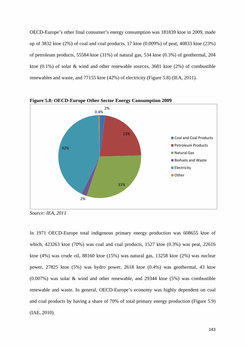
143
OECD-Europe’s other final consumer’s energy consumption was 181839 ktoe in 2009, made
up of 3832 ktoe (2%) of coal and coal products, 17 ktoe (0.009%) of peat, 40833 ktoe (23%)
of petroleum products, 55584 ktoe (31%) of natural gas, 534 ktoe (0.3%) of geothermal, 204
ktoe (0.1%) of solar & wind and other renewable sources, 3681 ktoe (2%) of combustible
renewables and waste, and 77155 ktoe (42%) of electricity (Figure 5.8) (IEA, 2011).
Figure 5.8: OECD-Europe Other Sector Energy Consumption 2009
Source: IEA, 2011
In 1971 OECD-Europe total indigenous primary energy production was 608655 ktoe of
which, 423263 ktoe (70%) was coal and coal products, 1527 ktoe (0.3%) was peat, 22616
ktoe (4%) was crude oil, 88160 ktoe (15%) was natural gas, 13258 ktoe (2%) was nuclear
power, 27825 ktoe (5%) was hydro power, 2618 ktoe (0.4%) was geothermal, 43 ktoe
(0.007%) was solar & wind and other renewable, and 29344 ktoe (5%) was combustible
renewable and waste. In general, OECD-Europe’s economy was highly dependent on coal
and coal products by having a share of 70% of total primary energy production (Figure 5.9)
(IAE, 2010).
2%
23%
31%
2%
42%
0.4%
Coal and Coal Products
Petroleum Products
Natural Gas
Biofuels and Waste
Electricity
Other
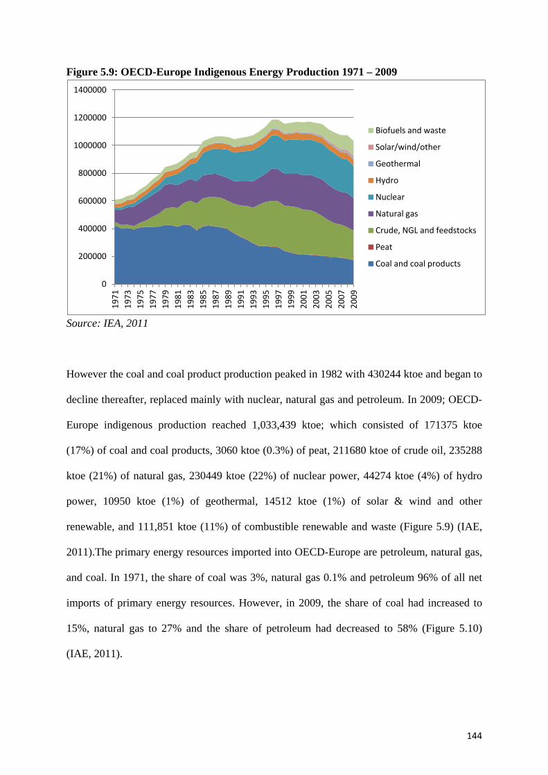
144
Figure 5.9: OECD-Europe Indigenous Energy Production 1971 – 2009
Source: IEA, 2011
However the coal and coal product production peaked in 1982 with 430244 ktoe and began to
decline thereafter, replaced mainly with nuclear, natural gas and petroleum. In 2009; OECD-
Europe indigenous production reached 1,033,439 ktoe; which consisted of 171375 ktoe
(17%) of coal and coal products, 3060 ktoe (0.3%) of peat, 211680 ktoe of crude oil, 235288
ktoe (21%) of natural gas, 230449 ktoe (22%) of nuclear power, 44274 ktoe (4%) of hydro
power, 10950 ktoe (1%) of geothermal, 14512 ktoe (1%) of solar & wind and other
renewable, and 111,851 ktoe (11%) of combustible renewable and waste (Figure 5.9) (IAE,
2011).The primary energy resources imported into OECD-Europe are petroleum, natural gas,
and coal. In 1971, the share of coal was 3%, natural gas 0.1% and petroleum 96% of all net
imports of primary energy resources. However, in 2009, the share of coal had increased to
15%, natural gas to 27% and the share of petroleum had decreased to 58% (Figure 5.10)
(IAE, 2011).
0
200000
400000
600000
800000
1000000
1200000
1400000
1971
19
73
1975
19
77
1979
19
81
1983
19
85
1987
19
89
1991
19
93
1995
19
97
1999
20
01
2003
20
05
2007
20
09
Biofuels and waste
Solar/wind/other
Geothermal
Hydro
Nuclear
Natural gas
Crude, NGL and feedstocks
Peat
Coal and coal products

145
Figure 5.10: OECD-Europe Net Energy Imports 1971 – 2009
Source: IEA, 2011
In 1971, OECD Europe total final energy consumption was 919,171 ktoe. This consisted of
203618 ktoe (23%) of coal and coal products, 727 ktoe (under 1%) of peat 507959 ktoe
(56%) of oil products, 61980 ktoe (9%) natural gas, 306 ktoe (under 1%) of geothermal,
26820 ktoe (3%) combustible renewable, and 99819 ktoe (11%) electricity (IAE, 2011).
However during the period 1971 to 2008 the structure of final consumption has changed
somewhat so that in 2009, total final energy consumption was 1,226,984 ktoe; consisting of
48,283 ktoe (4%) of coal and coal products, 355 ktoe (under 1%) of peat, 4345 ktoe (under
1%) of petroleum, 533,207 ktoe (44%) of oil products, 263,328 ktoe (21%) natural gas, 2755
ktoe (under 1%) of geothermal, 1524 ktoe (under 1%) of solar & wind and other renewables,
71205 ktoe (6%) of combustible renewable and waste, and 255219 ktoe (21%) of electricity
(Figure 5.11) (IAE, 2011).
0
100000
200000
300000
400000
500000
600000
700000
800000
900000
Coal and coal products Crude, NGL and feedstocks Natural gas
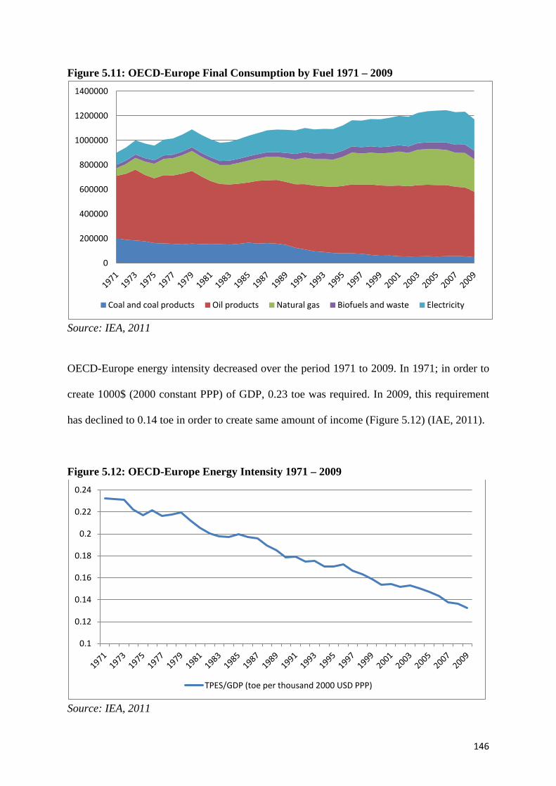
146
Figure 5.11: OECD-Europe Final Consumption by Fuel 1971 – 2009
Source: IEA, 2011
OECD-Europe energy intensity decreased over the period 1971 to 2009. In 1971; in order to
create 1000$ (2000 constant PPP) of GDP, 0.23 toe was required. In 2009, this requirement
has declined to 0.14 toe in order to create same amount of income (Figure 5.12) (IAE, 2011).
Figure 5.12: OECD-Europe Energy Intensity 1971 – 2009
Source: IEA, 2011
0
200000
400000
600000
800000
1000000
1200000
1400000
Coal and coal products Oil products Natural gas Biofuels and waste Electricity
0.1
0.12
0.14
0.16
0.18
0.2
0.22
0.24
TPES/GDP (toe per thousand 2000 USD PPP)

147
On the other hand, OECD-Europe household energy consumption increased over the period
1971 to 2009, reflecting the more energy dependent life styles. In 1971, a household
consumed an average of 2.77 toe where in 2008 this figure had increase to 3.18 toe (Figure
5.13) (IAE, 2011).
Figure 5.13: OECD-Europe Energy Consumption per Person 1971 – 2009
Source: IEA, 2011
5.3 Overview of OECD-Europe Natural Gas Market
Natural gas is an important resource fuel for Europe and it is expected to remain important in
the next few decades (Holz et al., 2006; EIA, 2009 and IEA, 2010b) due to increasing
environmental concerns and related policies. In particular, the increasing use of natural gas in
electricity generation is expected to continue given the lower carbon intensity of natural gas
relative to other fossil fuels and its relative fuel efficiency (EIA, 2009 and IEA, 2010d). At
the same time, indigenous natural gas production in Europe is declining; hence, Europe’s
natural gas import dependence is expected to increase (Honore, 2006 and Remme et al.,
2008) and accurate forecasts of future natural gas demand are necessary to assess the scale of
this dependency.
2.5
2.7
2.9
3.1
3.3
3.5
1971 1973 1975 1977 1979 1981 1983 1985 1987 1989 1991 1993 1995 1997 1999 2001 2003 2005 2007 2009
TPES/Population
TPES/Population

148
It is important to put the expected growth in OECD-Europe’s natural gas demand and import
dependency in a global perspective for appreciating their impact on OECD-Europe’s energy
security. Due to the abovementioned advantages, EIA (2009) expects that the power sector
will consume 35% of the world’s total natural gas consumption by 2030 compared to 32% in
2006. Although Europe’s neighbouring regions have substantial reserves and resources
(Hafner et al. 2009), there is also increasing demand for natural gas in developing countries,
in particular China. Increasing demand for natural gas puts pressure on Chinese officials to
actively penetrate the Caspian Region, develop infrastructure and contractual solutions and
import natural gas (Hall and Grant, 2009; Remme et al., 2008). In recent years, China has
developed effective policy tools for both oil and natural gas and provided package solutions
covering finance, field development, and pipeline construction. As a result, China has gained
direct access to Caspian energy sources and secured long-term production sharing
agreements. There is, therefore, also global competition for accessing energy resources and
this competition puts pressure on OECD-Europe to develop necessary measures to secure
natural gas for its future needs. In this respect, identification of future natural gas needs is a
vital and urgent issue for policy makers in OECD-Europe (Christoffersen, 1998 and Bilgin
2009).
While the demand for natural gas is expected to rise globally, the resources are not
geographically distributed equally. The largest natural gas reserves are located in the Russian
Federation (48,000 billion cubic metres, bcm), Iran (28,000 bcm) and Qatar (26,000 bcm). In
2004, these three countries account for 58% of proven global natural gas reserves (BP, 2005).
Furthermore, the Gas Exporting Countries Forum (GECF), which was created in 2001, has
become another concern for net importers of natural gas, since in future the GECF might act
as a cartel to gain control over the gas supplies and prices (Stern, 2002).

149
Hence, on the demand side, the global competition for natural gas is getting increasingly
fierce and on the supply side, the natural gas resources are concentrated in a limited number
of countries that may establish a powerful cartel. Not surprisingly, these developments create
anxiety across an import dependent Europe (see, for example, EC, 2009). Volatility in the
natural gas prices or supply can have devastating effects on European economies.
According to Bilgin (2009), Europe could possibly diversify its natural gas suppliers by
including Middle Eastern and Caspian sources (such as Iran, Iraq, Azerbaijan, Algeria, Egypt,
and Turkmenistan). Despite their relative market power over their clients, the suppliers of
natural gas also compete for accessing a diverse mix of markets in order to minimize the
uncertainty over their export revenues (Shaffer, 2010, Nichol, 2009 and Denison, 2009). For
instance, Caspian Region countries such as Turkmenistan, Kazakhstan, and Azerbaijan share
the same interests with Europe for exporting their gas through non-Russian transport routes
(Shaffer, 2010, Nichol, 2009 and Denison, 2009). Hence, both OECD-Europe and the
Caspian suppliers might benefit from diversification of Europe’s natural gas procurement.
On the other hand, there are also some difficulties related to diversification of OECD-
Europe’s natural gas procurement. Firstly, it is important to highlight that natural gas is
transported either via pipelines or in the LNG form. When operating costs are taken into
account, pipelines often provide a more efficient alternative (Hanfer et al., 2008). According
to Pirani et al. (2009), in 2008, 90% of European natural gas imports were delivered via
pipelines. For this reason, energy security issues cover investments on necessary
infrastructure and the energy security of transit countries as well.

150
The importance of transit countries has become evident during the Russia-Ukraine gas
conflict in 2006 and in 2009. Even though it is frequently argued that there were hidden
political motives, the main reason for this conflict appears to be related to price. Accordingly,
Russia was unwilling to continue subsidising the natural gas prices for Ukraine and the
Ukrainian economy struggled to pay the full price charged to Europe. As a result, Russia cut
natural gas supplies to Ukraine in January 2006 for three days and in January 2009 for nearly
three weeks.
Europe has experienced supply disruptions because of the abovementioned conflicts between
Russia and Ukraine. In particular, during the January 2009 conflict, exports to 16 EU member
states and Moldova decreased significantly on 6 January 2009 and cut totally from 7 January
2009. The countries hit by this supply disruption seriously in the Balkans, faced a
humanitarian emergency; a considerable share of the households in the Balkan region could
not be heated during coldest time of the year. Countries including Hungary and Slovakia also
experienced economic loss and problems because of this supply disruption (Pirani et al.,
2009). A staff working document published by the European Commission summarises
Europe’s vulnerability with respect to this matter, stating: “One quarter of all energy
consumed in the EU is gas. 58% of this gas is imported. Of this, 42% comes from Russia, and
around 80% of EU imports of gas from Russia pass via Ukraine.” (EC, 2009; p. 2).
It can be argued, therefore, that not only diversification of sources but also diversification of
transit routes has become imperative for OECD-Europe. The Nabucco project, 45 which
enables Europe to import gas from both the Middle East and Caspian resources, can help
45 Nabucco is 3,300 km pipeline project that will run from Turkey’s borders with Georgia and Iran to Baumgarten in Austria, along a route passing through Bulgaria, Romania and Hungary.

151
Europe to achieve both of these objectives; diversifying import source and transit routes of
natural gas (Holz et al. 2006). Feeling the need to respond, China’s long-term and
comprehensive institutional solutions for accessing to Caspian gas, EU and its financial
institutions have become actively involved in the Nabucco project. The Nabucco Summit was
held in Budapest on 27th of January 2009. The European Union’s political and financial
institutions including the European Bank of Reconstruction and Development (EBRD) and
European Investment Bank declared their support and, as a part of its economic recovery
plan, the European Commission proposed 250 million Euros to be contributed for funding the
project via the European Investment Bank (Nabucco Declaration, 2009 and Deutche Welle,
2009).
The second barrier related to diversification of OECD-Europe’s natural gas procurement is
the political power of Russia who, not surprisingly does not want to lose its share and market
power in the European natural gas market (Socor, 2008; Smith, 2010). Russian authorities are
strongly against the Nabucco project and similar formations. Russia advocates that Gazprom
is a reliable supplier and therefore diversification of transport routes will be sufficient for
Europe’s energy security (Socor, 2008). In this respect, Russian policy is to encourage
Caspian countries to divert their export routes to the east rather than west. Russia also uses its
political power to obstruct new European Union projects aiming to diversify import sources
including the Nabucco pipeline and instead, push forward a more expensive South Stream
project. The idea behind the South Stream project is to diversify the transport routes of
Russian gas to Europe so that reoccurrence of supply disruptions during the Russia-Ukraine
conflict can be avoided. From the perspective of Europe, however, South Stream does not
diversify the risks related to the import source (Pirani et al., 2010).

152
Further complications in the natural gas market involve the European Commission’s
objective to liberalize the natural gas sector. In the natural gas and other fuel markets, a major
consideration for liberalisation efforts is the use of long-term contracts. These generally
involve take-or-pay obligations between 80-90% of the annual contract quantity, often for a
period between 15 to 20 years. When most transactions occur in long-term basis the market is
expected to lose from its competitiveness (Newbery, 1984). As a part of the undergoing
efforts for liberalization of the downstream wholesale market and of gas distribution, long-
term natural gas supply contracts in Europe (which are generally issued for 20-25 years) are
expected to be issued for shorter periods such as 8-15 years (Kavalov et al, 2009).
That said, it has also been argued that long-term contracts will still dominate over the next
two decades but with more flexible price options (Stern, 2002; see also Neuhoff and von
Hirschhausen, 2005). Neuhoff and von Hirschhausen (2005) argue that suppliers’ preference
for long-term contracts depend on the difference between short run and long run price
elasticities of demand. If the long-run elasticity is significantly higher than the short run
elasticity, the suppliers prefer long-term contracts. It has also been argued that longer-term
contracts may be socially beneficial if they facilitate infrastructure investments that appear to
be much riskier with spot transactions and price volatility (Oren, 2003).
Overall, from the perspective of energy security of OECD-Europe several issues appear to be
important. Natural gas will remain an important fuel over the coming decades, largely due to
its central role in power generation. Both global and European demand for natural gas will be
increasing. On the supply side, OECD-Europe’s indigenous production will be declining
while the global suppliers that are already low in number may initiate cartel-like
organisations. Although OECD-Europe can diversify its suppliers by accessing Middle

153
Eastern and Caspian gas, this would require investments in pipeline projects, which would
lead to diplomatic struggles against the political power of Russia and would probably involve
binding long-term purchase agreements. Arguably, reliable energy forecasts are essential for
analysing all these aspects. They are necessary for policy makers, energy planning and
regulative bodies for adopting the policies and measures that are necessary for delivering
energy security of OECD-Europe.
Future natural gas demand is also very important for energy providing firms and financial
institutions in order to assess multibillion-dollar investment projects. Uncertainty about the
future could make such investment decisions risky, delaying investment decisions. The
natural gas producing countries and their national energy companies such as Russia and
Gazprom are often criticized for being late in their investments, and these criticisms arouse
the concerns about the supply security. If Gazprom fails to meet future natural gas demand, it
might lose its position as a reliable supplier. Thus, reliable demand projections are also vital
to natural gas producers for protecting their position as reliable suppliers.
As discussed above identifying the main drivers of natural gas and forecast future natural gas
demand can provide number of benefits to policy makers of both natural gas importing and
exporting countries and energy companies by minimizing the uncertainty about the future,
identifying the price-income elasticities and UEDTs. In the next section, previous natural gas
demand studies are discussed.

154
5.4 Review of Studies Focussing on OECD Europe Natural Gas Demand
In this section, the key literature is discussed in two main parts. Firstly, previous studies that
have estimated natural gas demand elasticities are reviewed. Secondly, previous projections
for future natural gas consumption are summarised.
5.4.1 Previous Studies on Price and Income Elasticities of Natural Gas Demand
Pindyck (1979) analysed the structure of world energy demand for different fuels and sectors
for nine OECD countries including Belgium, Canada, France, Italy, Netherlands, Norway,
Sweden, Switzerland, UK, West Germany, and US over the period 1955-1972. He found
estimated natural gas price elasticities for residential and industrial sectors ranging from -0.9
to -1.8 and -0.41 to -2.34 respectively. Griffin (1979) investigated natural gas demand
functions for different sectors of 18 OECD countries including Austria, Belgium, Canada,
Denmark, France, West Germany, Greece, Ireland, Italy, Japan, Netherlands, Norway, Spain,
Sweden, Switzerland, Turkey, United Kingdom and US over the period 1955 to 1974. He
concluded that the price elasticity of natural gas varied between -0.83 to -1.60.
Estrada and Fugleberg (1989) investigated the price responsiveness of natural gas demand for
West Germany and France and found estimated price elasticities varying between -0.75 and -
0.82 for West Germany and from -0.61 to -0.76 for France. Nilsen et al. (2005) examined
natural gas demand per capita in 12 European countries including Austria, Belgium,
Denmark, Finland, France, Germany, Ireland, Italy, Netherlands, Spain, Switzerland, and UK
over the period 1978-2002. Their results suggest that the short run and long run price
elasticities vary between 0 to -0.3 and 0 to -0.6 respectively, whereas the short and long run
income elasticities range from 0.3 to 0.7 and 1.9 to 2.2 correspondingly.

155
There are also some survey studies, which investigate the price and income elasticities of
natural gas demand. The summary of these surveys are given in Table 5.2.
Table 5.2: Summary of Estimated Natural Gas Demand Surveys Survey Short Run
Price Elasticity
Short Run Income Elasticity
Long Run Price Elasticity
Long Run Income Elasticity
Taylor (1977) 0 to -0.38 0.01 to 1 0 to -3.85 -0.29 to 3.11 Bohi (1981) 0.09 to -0.50 -0.03 to 0.05 0.33 to -2.42 0.02 to 2.18
Kirby (1983) - - -0.3 0.4
Bohi and Zimmerman (1984) 0.16 to -0.63 0.02 to 0.78 0.99 to -3.44 0.09 to 3.08
Dahl (1993) 0.02 to -1.63 -0.33 to 1.74 1.56 to -10 -2.19 to 4.46
Overall, these previous studies and surveys suggest a wide range of price and income natural
gas elasticities. One reason for this might be previously applied models are insufficient in
terms of identifying the structural changes in natural gas demand. Hence, as stated before,
one of the aims in this work is to attempt to overcome some of the shortcomings of previous
studies by attempting to identify key structural changes in OECD-Europe natural gas demand
behaviour by using the UEDT/STSM approach. However, before this, studies focusing on
European natural gas demand projections are reviewed in the next section.
5.4.2 Previous Projections of European Gas Demand
There appear to have been few academic authors and institutions working on natural gas
demand projections. Mackay and Probert (1995), one of the early studies, predicted that
French natural gas demand will be somewhere between 46 – 58 bcm (38-43 million tonnes of
oil equivalent, mtoe)46 by 2010.47 According to Eurogas (2010), natural gas demand of EU-
46 Mackay and Probert (1995) present their natural gas projections in mtoe; the bcm figures are based upon the IEA conversion factor of 1 mtoe = 1.2125 bcm (IEA, 2010b).
156
27 would be between 535-562 bcm (482-507 mtoe) in 2020. However, this is somewhat
lower than Eurogas’s previous (Eurogas, 2007) where they projected EU natural gas demand
to be 641 bcm (578 mtoe) in 2020.48
Honore (2006) focuses on EU-25 natural gas demand by the power sector and concludes that
in 2015 natural gas demand by the power sector and the non-power sector would be 195 bcm
and 406 bcm (161 mtoe and 335 mtoe) respectively; a total of 601 bcm (496 mtoe).49There
are two institutions, the US Energy Information Administration (EIA) and the International
Energy Agency (IEA) that produced annual forecasts for OECD-Europe. EIA (2010b)
projected that OECD-Europe natural gas demand would be between 575 and 609 bcm (474
and 502 mtoe)50 by 2020, whereas IEA (2010b) predicted that OECD-Europe natural gas
demand would be somewhere between 534 and 589 bcm (440 and 486 mtoe)51 by 2020.
However, both of these institutions reduced their reference case projections considerably
from previous forecasts in 2008; the EIA’s natural gas demand reference scenario projection
for 2020 was 644 bcm (531 mtoe) and for the IEA was 699 bcm (576 mtoe) (EIA, 2008 and
IEA, 2008). The differences are illustrated in Figure 5.14.
47 Which looks to be a little high given that French natural gas consumption was 40 bcm (33 mtoe) in 2008 (IEA, 2011).
48 Eurogas (2010) and Eurogas (2007) present their natural gas projections in mtoe; the bcm figures are based upon the conversion factor of 1 mtoe = 1.11 bcm (as it is used in Eurogas publications).
49 Honore (2006) present their natural gas projections in bcm; the mtoe figures are based upon the IEA conversion factor of 1 mtoe = 1.2125 bcm (IEA, 2010d).
50 EIA (2010) present their natural gas projections in tcf, these figures have first been converted to bcm and then to mtoe based upon the IEA conversion factor of 1 mtoe = 1.2125 bcm (IEA, 2010d).
51 IEA (2010a) present their natural gas projections in both bcm and mtoe.

157
Although it is not possible to compare the above studies directly,52 it is clear that there is a
wide range of projections related to European natural gas demand. One reason might be the
dynamic structure of European natural gas demand that makes it difficult to minimize the
uncertainty about the future. This study therefore attempts to help uncover the structural
changes in the European natural gas market and help to reduce the uncertainty by utilizing the
STSM with the UEDT explained in previous chapters.
Figure 5.14: IEA and EIA OECD-Europe Natural Gas Demand Projections for 2020
5.5 Empirical Framework
As discussed in Chapter 3, it is assumed that OECD-Europe natural gas demand is identified
by:
𝐺𝑡 = 𝑓(𝑌𝑡 , 𝑃𝑡, 𝑈𝐸𝐷𝑇𝑡) (5.1)
52 This is primarily due to the differences in country groups, but also the different definitions and conversion factors used.
400
450
500
550
600
650
2008 2009 2010
bcm
Year Projection was Made
Reference case of International Energy Agency-IEA
Reference Case of Energy Information Administartion-EIA

158
Where: Gt = OECD-Europe total natural gas demand;
Yt = GDP (US Dollar 2000=100 PPP)
Pt = OECD Europe natural gas price index (2005=100); and
𝑈𝐸𝐷𝑇𝑡 = Underlying Energy Demand Trend for OECD-Europe Natural Gas.
5.6 Data
Annual time series data from 1978-2009 for E (natural gas consumption ktoe), Y (GDP 2000
constant US dollar-PPP) and P (OECD-Europe Real natural gas price index 2000 =100) are
used for the analysis (Figure 5.15). All variables are obtained from the International Energy
Agency (IEA, 2011).
Figure 5.15: Natural Log of OECD-Europe Price, GDP, and Natural Gas Consumption 1978-2009
1980 1985 1990 1995 2000 2005 2010
12.50
12.75
13.00
13.25Natural Gas Consumption (ktoe)
1980 1985 1990 1995 2000 2005 2010
9.00
9.25
9.50GDP (2000 constant US $)
1980 1985 1990 1995 2000 2005 2010
4.50
4.75
Natural Gas Price Index (2000 constant US $)

159
5.7 Estimation Results
The final preferred equation resulting from the estimation procedures outlined above is given
in Table 5.3 and Figure 5.16 along with the diagnostics. It can be seen that the preferred
model passes all the diagnostic tests including the additional normality tests for the auxiliary
residuals generated by the STSM approach, with limited estimated dynamic terms. The
estimated impact elasticities for both income and price are zero, whereas the estimated long
run income elasticity of 1.16 and the estimated long run and price elasticity of -0.17 come
through after a lag of one year.
The estimated UEDT from this procedure is a local level model without a slope, but despite
this the estimated UEDT illustrated in Figure 5.17 and summarised in Table 5.4 is clearly
non-linear given the estimated level hyper-parameter; with periods when it increased and
periods when it is decreased, with a sharp decrease after 2004.
As explained in the methodology section, in order to illustrate the UEDT’s importance
relative to income and price, their estimated contributions to the change in OECD-Europe
natural gas demand are estimated using the method proposed by Broadstock and Hunt (2010)
by decomposing the change in natural gas demand as follows:
∆𝑔𝑡� = 1.164∆𝑦𝑡−1 − 0.171∆𝑝𝑡−1 + ∆𝑈𝐸𝐷𝑇𝑡� (5.2)
The decomposition is shown in Figure 5.18 and summarised in Table 5.5. This shows that
since 1979 income was the main driver of OECD-Europe natural gas demand closely
followed by the UEDT. In contrast, the estimated contribution from price is relatively small.

160
Table 5.3: OECD-Europe Total Natural Gas Demand STSM Estimates and Diagnostics Sample 1978-2009 Variables Coefficients Std.Error Probabilities yt-1 1.1642 0.21532 0.000 pt-1 -0.1709 0.07480 0.030 Lvl1988 -0.0881 0.03276 0.012 Hyperparameters: Goodness of fit: Level: 0.00079 p.e.v 0.0007 Irregular: 0.00000 p.e.v/m.d.2 1.2799 R2 0.9918 UEDT2009: 2.9453 Rd
2 0.4066 Diagnostics Residuals: Auxiliary Residuals: Irregular Level Std. Error 0.90 Std. Error 0.90 0.98 Normality 0.66 Normality 0.89 0.86 Skewness 0.42 Skewness 0.64 0.60 Kurtosis 0.67 Kurtosis 0.93 0.91 H(9) 0.76 r(1) 0.17 Nature of Trend: Local Level r(5)
-0.05
Q(5,4) 1.41 Predictive Tests(2002-2009) LR TEST 24.5186 (0.000) Failure 0.47 Cusum t(8) 1.64
Notes: -See notes to Table 4.353 -Model includes a level intervention for the year 1988; - LR Test represents a likelihood ratio tests on the same specification after imposing a fixed level and no slope hyperparameter and distributed as 𝜒(1)
2 and probabilities are given in parenthesis.
-Failure is a predictive failure statistic distributed as 𝜒(8)2 and Cusum is a mean stability statistic
distributed as the Student t distribution; both are STAMP prediction tests found by re-estimating the preferred model up to 2000 and predicting for 2001 thru 2009;
53For simplicity and to save space the notes given in the previous table are not repeated again.

161
Figure 5.16: Prediction Graphics of European Natural Gas Demand 2001-2009
Figure 5.17: The Estimated OECD-Europe Natural Gas UEDT
2002 2003 2004 2005 2006 2007 2008 2009
13.1
13.2
13.3Actual e Prediction e
2002 2003 2004 2005 2006 2007 2008 2009
0
2Standardised residuals
2002 2003 2004 2005 2006 2007 2008 2009
-5
0
5Cusum
1980 1985 1990 1995 2000 2005
2.825
2.850
2.875
2.900
2.925
2.950
2.975
3.000
3.025UEDT for OECD- Europe natural gas demand

162
Table 5.4: The Average Annual Change of the UEDT
Period Average Annual Change of UEDT
1979-1989 - 0.0096 1989-1999 0.0134
1999-2009 - 0.0059
1979-2009 - 0.0007
Figure 5.18: Estimated Contributions to the Annual Percentage Change in OECD-Europe Natural Gas Demand
Table 5.5: Summary of the Estimated Contributions to the Average Percentage per Annum Change in OECD-Europe Natural Gas Demand
Period Contribution from: Total change
in Gas Demand Income Price UEDT
1979-1989 2.62 -0.17 -0.96 1.50 1989-1999 2.57 -0.01 1.34 3.90 1999-2009 2.76 -0.86 -0.59 1.31 1979-2009 2.65 -0.34 -0.07 2.24 Note: Following from Equation (5.2) the estimated annual changes per annum contributions are approximated as follows: ((1.164𝛴∆𝑦𝑡−1)/𝑛)%, ((−0.171𝛴∆𝑝𝑡−1)/𝑛)% and ((𝛴𝑈𝐸𝐷𝑇𝑡� /𝑛)%- for the contributions of income, price, and the UEDT respectively. (The total change being approximated by (𝛴∆𝑔𝑡� /𝑛)%.) Where n is the span of years that the change is calculated.
-0.1
-0.05
0
0.05
0.1
0.15
1980
19
81
1982
19
83
1984
19
85
1986
19
87
1988
19
89
1990
19
91
1992
19
93
1994
19
95
1996
19
97
1998
19
99
2000
20
01
2002
20
03
2004
20
05
2006
20
07
2008
20
09
Income Contribution Price Contribution UEDT Contribution ∆g

163
To show this more clearly, the contributions are re-calculated in absolute terms, presented as
shares in Figure 5.19 54 and summarised in Table 5.6. This shows that the share of the
contribution of income is the largest and generally, increases over the estimation period. The
second largest share is clearly the UEDT, which was at its highest in the 1990s when it was
making a positive contribution (see Table 5.5) compared to the 1980s and the 2000s when it
was making a negative contribution. Price clearly makes the smallest contribution. Given the
relative importance of the UEDT, it should arguably be taken into account when modelling
and forecasting OECD-Europe natural gas demand. The preferred estimated equation will
therefore now be used to construct future scenarios for OECD-European natural gas demand,
as explained in the next section.
Figure 5.19: Estimated Shares of the Contributions to the Change in OECD-Europe Natural Gas Demand
54The absolute value of the estimated contribution of each factor is divided by the sum of the absolute values of all estimated contributions of the factors; e.g.
𝐶𝑜𝑛𝑡𝑟𝑖𝑏𝑢𝑡𝑖𝑜𝑛 𝑠ℎ𝑎𝑟𝑒 𝑜𝑓 𝑦𝑡 = │𝐸𝑠𝑡. 𝑐𝑜𝑛𝑡. 𝑜𝑓𝑦𝑡││𝐸𝑠𝑡. 𝑐𝑜𝑛𝑡. 𝑜𝑓𝑦𝑡│+│𝐸𝑠𝑡.𝑐𝑜𝑛𝑡. 𝑜𝑓𝑝𝑡│+│𝐸𝑠𝑡. 𝑐𝑜𝑛𝑡. 𝑜𝑓𝑈𝐸𝐷𝑇𝑡│
.
0%
10%
20%
30%
40%
50%
60%
70%
80%
90%
100%
1980
19
81
1982
19
83
1984
19
85
1986
19
87
1988
19
89
1990
19
91
1992
19
93
1994
19
95
1996
19
97
1998
19
99
2000
20
01
2002
20
03
2004
20
05
2006
20
07
2008
20
09
Share of Income Contribution Share of Price Contribution Share of UEDT Contribution

164
Table 5.6: Summary of the Estimated Shares of the Contributions to the Change in OECD-Europe Natural Gas Demand
Period Average shares of contribution from: Income Price UEDT
1979-1989 41.2% 24.3% 34.6% 1989-1999 47.0% 13.8% 39.2% 1999-2009 52.8% 18.6% 28.6% 1979-2009 47.0% 18.9% 34.1% Note: The shares of the contributions to the change in OECD-Europe Natural Gas Demand per annum are approximated as follows:
(( │1.164Σ∆𝑦𝑡−1│
│1.164Σ∆𝑦𝑡−1│+│−0.171Σ∆𝑝𝑡−1│+│Σ∆𝑈𝐸𝐷𝑇𝑡│� )/𝑛) × 100,
(( │−0.171Σ∆𝑝𝑡−1│
│1.164Σ∆𝑦𝑡−1│+│−0.171Σ∆𝑝𝑡−1│+│Σ∆𝑈𝐸𝐷𝑇𝑡│� )/𝑛)) × 100, and
(( │Σ∆𝑈𝐸𝐷𝑇𝑡│�
│1.164Σ∆𝑦𝑡−1│+│−0.171Σ∆𝑝𝑡−1│+│Σ∆𝑈𝐸𝐷𝑇𝑡│� )/𝑛) × 100 for the shares of the contributions of income,
price, and the UEDT respectively. Where n is the span of years that the change is calculated.
5.8 Forecast Assumptions
This section outlines the assumptions about the future UEDT and other variables that are used
to construct the scenarios and presents the forecast results based on these assumptions. Three
scenarios are implemented in this chapter, namely ‘high’ case, ‘reference’ and ‘low ‘case as
discussed in methodology section.
In the ‘reference’ scenario, it is assumed that real natural gas OECD Europe prices will
increase 1.5% annually over period 2010-2020. The average annual prices increase is around
2% over the estimation period, however, for the future, the price increase is assumed slightly
less than before. The increase of GDP is expected to be 1% for 2010 and 2011 and a 2% per
annum thereafter. The average annual increase of GDP is around 2% over the estimation
period. Hence, it is assumed that after the global crises, GDP will increase 2% annum. For the
UEDT55, a slope of -0.004 is projected for the period 2009-2020. Although the average 55 Although the estimated slope of UEDT is zero over the estimation period, in order to create future values of UEDT, a series of slope values for UEDT is assumed based on the estimated past values of the UEDT and future expectations.

165
decrease of UEDT is -0.006 for the last decade (Table 5.5), it is expected that because of
environmental concerns, there might be some new regulations that encourages the
consumption of natural gas especially in the power sector.
In the ‘high’ case scenario, the natural gas price is assumed to increase 0.5% annually for the
period 2010 and 2020 (less than the increase observed over the estimation period).
Furthermore, it is assumed that GDP will increase 1.5% increase for both 2010 and 2011 and
will increase 2.5% per year thereafter to 2020. In the high case scenario, it is assumed that the
transformation of power sector to natural gas will be much higher than the reference case
hence it is assumed that the UEDT has a slope of -0.002 over the forecast period.
In the ‘low’ case scenario, it is assumed that the rise in natural gas prices will be 2% per
annum (similar with the estimation period). For GDP it is assumed to increase 0.5% for both
2010 and 2011 because of the global economic crises and then increase annually 1% per year
(lower than the estimation period average) until 2020. For the UEDT, it is assumed that it will
have a slope of -0.006 per annum (same as it was observed for 2000 and 2009) between 2010
and 2020. A graphical presentation of the scenario assumptions for GDP, real natural gas
price index, and the UEDT are illustrated in Figure 5.20.

166
Figure 5.20: Forecast Scenarios for Price, GDP, and UEDT
5.9 Forecast Results
The three scenarios up to 2020 are illustrated in Figure 5.21. These show that OECD Europe
natural gas demand is predicted to grow to 536, 585 and 644 bcm (442, 482 and 531 mtoe) by
2020 according to the low reference and high case scenarios respectively.
2000 2005 2010 2015 202010500115001250013500145001550016500 GDP (billion 2000 constant US $ PPP)
GDP High Case GDP Reference Case GDP Low Case
2000 2005 2010 2015 202025
50
75
100
125
150
175 Natural Gas Price Index (2005=100) Price Index High Case
Price Index Reference Case Price Index Low Case
2000 2005 2010 2015 2020
2.8802.9052.9302.9552.9803.0053.030
UEDT for OECD Europe Natural Gas Demand UEDT Low Case
UEDT Reference Case UEDT High Case

167
Figure 5.21: OECD Europe Natural Gas Demand Forecast Scenarios
5.10 Conclusion and Further Discussion
This chapter estimates an OECD-Europe Natural gas demand function by using the STSM
over the period 1978-2009. As far, as is known this is the first attempt to estimate a non-
linear UEDT for OECD-Europe natural gas demand. The results suggest the following:
i) In order of importance, Income, the UEDT, and real natural gas prices are all
factors that shape European natural gas demand.
ii) The income and the price elasticities are 1.16 and -0.17 respectively.
iii) Income has a greater impact on OECD-Europe natural gas demand than price and
this finding is consistent with previous studies.
iv) The UEDT has a stochastic process that increases and decreases over the
estimation period; however starting from 2004, it follows a decreasing path,
2000 2005 2010 2015 2020
450
500
550
600
650OECD Europe Natural Gas Demand (bcm) Low Case
Reference Case High Case

168
perhaps due to improved energy efficiency standards. However the environmental
concerns make natural gas a popular choice rather than other fossil fuels for power
generation, therefore it is expected that the power sector will widely use natural
gas as a fuel in the future, which might change the direction of UEDT to upward.
v) OECD-Europe natural gas demand is expected to be 536, 585 and 644 bcm (442,
482 and 531 mtoe) by 2020, according to the generated low, reference and high
case scenarios.
In summary, given its relative importance, the UEDT should be taken into account when
modelling OECD-Europe natural gas demand in addition to the main driver, income, and
price. Arguably, the UEDT has important information that is of value to European
decision makers when developing gas security policies.
As discussed in previous sections, some of the main challenges of OECD-Europe in terms
of natural gas are import dependency and increasing global demand for natural gas,
security and diversity of gas supply, liberalization of natural gas markets and investment
requirements of the gas sector. For policy makers, energy companies and financial
institutions alike, it is important to minimize the uncertainty around future natural gas
demand in order to establish appropriate energy security measures. This research
contributes in this area by identifying the structure and composition of OECD-Europe
natural gas demand and its responsiveness to its main determinants and provides
invaluable information for the stakeholders.

169
CHAPTER 6: US Gasoline Demand∗
6.1 Introduction
As outlined in the methodology above, in this chapter a US per capita gasoline demand
function is estimated with annual data over the period 1949-2008 using an extended version
of the STSM/UEDT approach that includes asymmetric price responses and time varying
parameters (TVP). As far as is known, this is the first attempt to estimate an energy demand
relationship that incorporates a stochastic UEDT and asymmetric price responses within a
TVP framework.
World demand for oil increased rapidly until 2008. As a result of this increase, the market
produced crude oil prices that went beyond their highest peak of the early 1980s (Huntington,
2010). One reason being the growth in oil demand was not met by production increases with
OPEC spare capacity decreasing to historically low levels; thus leaving the world market in a
weak position against supply shocks (IMF, 2005, and Huntington, 2010). Coupled with the
fast oil demand growth was the resultant increase in GHG emissions – that contribute towards
global climate change.
The security of oil supply and the related economic vulnerability along with the
environmental concerns put pressure on policy makers to deal with these problems. Before
assessing any policy implications such as carbon taxes, vehicle efficiency standards, cap and
trade schemes, and reducing oil vulnerability, it is vital that the factors affecting oil demand ∗Earlier preliminary work for this chapter was presented at the following:
• 33rd IAEE international Conference: The Future of Energy Global Challenges, Diverse Solutions. Rio De Janeiro, Brazil 6-9 June 2010; and
• 3rd International Workshop on Empirical Methods in Energy Economics, University of Surrey, Guildford, UK 24-25 June 2010.

170
are investigated (Huntington, 2010) and a key part of this investigation is to obtain
information on the key price and income elasticities of oil demand. Consequently, there have
been many previous studies of US Gasoline demand in order to estimate price elasticities.
However, no previous study, as far as is known, has attempted to capture the impact of
unobserved factors (via a UEDT) and asymmetric price responses, while also experimenting
to see whether or not the price and income elasticities change over time. The research for this
chapter therefore attempts to rectify this omission.
In summary, the key motivations for this chapter are as follows:
i) to estimate time varying income and asymmetric price elasticities for US per-capita
gasoline demand;
ii) to uncover the UEDT for US per-capita gasoline demand;
iii) to investigate if/how the parameters of the model change over time;
iv) produce forecast scenarios for US per-capita gasoline demand to 2020; and
v) to evaluate the findings in terms of policy application and assessment.
However, before these issues are addressed the next section sets the scene in terms of US
gasoline consumption and associated CO2 emissions before summarising the associated
literature.
6.2 An Overview of US Gasoline Consumption and CO2 Emissions
In 1971, the US economy generated 4291 Mt of CO2 while the world economies in total
generated 14096 Mt of CO2; therefore, in 1971 the US was individually responsible for 30%
of global CO2 emissions. Within this, the US transport sector produced 1081 Mt of CO2,
accounting for 25% of the total US CO2 emissions. In 2008, CO2 emissions created by the US

171
economy had increased to 5587 Mt, which accounted for 19% of global CO2 emissions of
29454 Mt (Figure 6.1) with the share of the US transport sector being 30%, producing1691
Mt of CO2 (Figure 6.2)(IEA, 2010c).
The US transport sector has historically had a big share of CO2 emissions (Figure 6.2);
moreover, in 2008 combusted oil products accounted for 1655 (98%) Mt of total 1691 Mt
CO2 emissions generated by the transport sector (IEA, 2010c).Given this large share of CO2
any US policies developed to attempt to curb CO2 and other GHG emissions and contribute
towards the halting of climate change should therefore address the consumption of oil
products in transport sector where the emissions emanate from.
Figure 6.1: US CO2 Emissions 1971-2008 (Mt.)
Source: IEA, 2010 The demand for US oil products increased from 431,423 ktoe to 781,703 ktoe from 1960 to
2008 with most of the demand generated by the transport sector. Furthermore, the demand for
oil products by the US transport sector increased from 225,242 ktoe (52%) to 565,116 ktoe
0%
10%
20%
30%
40%
50%
60%
70%
80%
90%
100%
1971
1973
1975
1977
1979
1981
1983
1985
1987
1989
1991
1993
1995
1997
1999
2001
2003
2005
2007
Rest of World
United States

172
(72%) for the same period (Figure6.3) (IEA, 2010c). This increase transformed the US
economy making it even more dependent on oil and oil products and consequently more
vulnerable to supply disruptions, thus raising serious concerns about US oil and energy
security.
Figure 6.2: Sectoral CO2 Emissions 1971- 2008 (Mt.)
Source: IEA, 2010
US CO2 emissions from the transport sector was also the fastest increasing source of GHG’s,
a net 47% increase between 1990 to 2006 (US EPA, 2010). US EPA (2006) illustrates that in
2003, light–duty vehicles (passenger cars, SUVs, Minivans, Pickup Trucks and Motorcycles)
fuelled by gasoline had a 62% share in transport sector GHG emissions and, moreover, it was
the fastest growing with a net increase of 20% between 1990 and 2003.This illustrates that
gasoline demand plays a significant role in terms of US GHG emissions.
0%
10%
20%
30%
40%
50%
60%
70%
80%
90%
100%
1971
1973
1975
1977
1979
1981
1983
1985
1987
1989
1991
1993
1995
1997
1999
2001
2003
2005
2007
Transport Residential Other Sectors Power Sector Industry
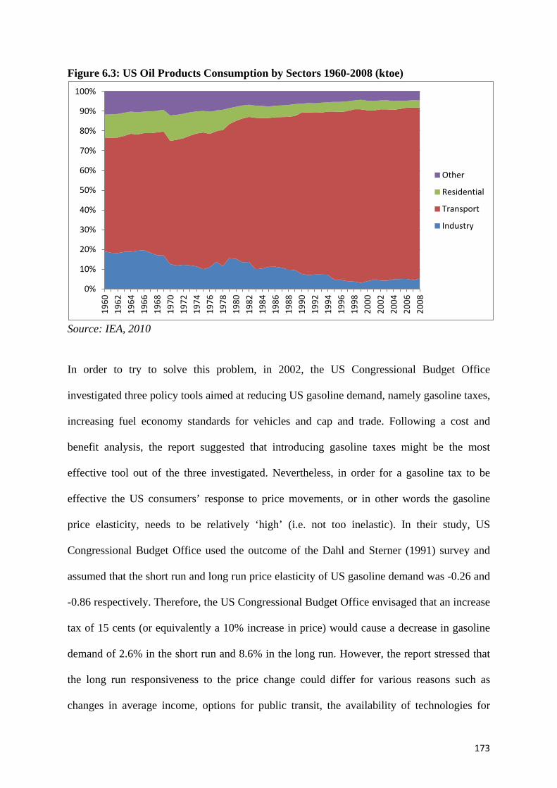
173
Figure 6.3: US Oil Products Consumption by Sectors 1960-2008 (ktoe)
Source: IEA, 2010
In order to try to solve this problem, in 2002, the US Congressional Budget Office
investigated three policy tools aimed at reducing US gasoline demand, namely gasoline taxes,
increasing fuel economy standards for vehicles and cap and trade. Following a cost and
benefit analysis, the report suggested that introducing gasoline taxes might be the most
effective tool out of the three investigated. Nevertheless, in order for a gasoline tax to be
effective the US consumers’ response to price movements, or in other words the gasoline
price elasticity, needs to be relatively ‘high’ (i.e. not too inelastic). In their study, US
Congressional Budget Office used the outcome of the Dahl and Sterner (1991) survey and
assumed that the short run and long run price elasticity of US gasoline demand was -0.26 and
-0.86 respectively. Therefore, the US Congressional Budget Office envisaged that an increase
tax of 15 cents (or equivalently a 10% increase in price) would cause a decrease in gasoline
demand of 2.6% in the short run and 8.6% in the long run. However, the report stressed that
the long run responsiveness to the price change could differ for various reasons such as
changes in average income, options for public transit, the availability of technologies for
0%
10%
20%
30%
40%
50%
60%
70%
80%
90%
100% 19
60
1962
19
64
1966
19
68
1970
19
72
1974
19
76
1978
19
80
1982
19
84
1986
19
88
1990
19
92
1994
19
96
1998
20
00
2002
20
04
2006
20
08
Other
Residential
Transport
Industry

174
improving fuel economy. Therefore, for the long run the assumption by the US Congressional
Budget Office was that suggested by the US Department of Energy of a long run price
elasticity of –0.38. However, this is smaller (in absolute terms) than the -0.86 from the Dahl
and Sterner (1991) survey. It is important therefore that well estimated robust estimates of the
price responsiveness (price elasticity) underpin this type of analysis. Consequently, one of the
main aims of this chapter is to re-estimate the US Gasoline price responsiveness (price
elasticity) and income responsiveness (income elasticity) using the structural time series
approach, and importantly assessing whether or not they are changing over time.
Before this, the next section reviews the literature specific to this chapter, namely time
varying parameters, asymmetric price responses and US gasoline demand studies.
6.3 Literature Review
6.3.1 Previously Estimated (Symmetric) Gasoline Demand Elasticities
A considerable amount of research has focussed on gasoline demand with a noteworthy
number of surveys summarizing the results; such as Taylor (1977) Bohi (1981), Kouris
(1983a), Bohi and Zimmerman (1984), Dahl (1986), Dahl and Sterner (1991), Goodwin
(1992), Dahl (1993), Espey (1998). The results and the main findings of these surveys are
summarized below (Table 6.1).
Overall, these surveys suggest a wide range of price and income elasticity estimates. Most of
the surveys, such as Bohi and Zimmerman (1984), Dahl (1986), Dahl and Sterner (1991),
suggest that the previously estimated models might be insufficient in terms of identifying
important structural changes. Hence, one of the aims of the research for this chapter is to
attempt to identify key structural changes in US gasoline demand behaviour by using the
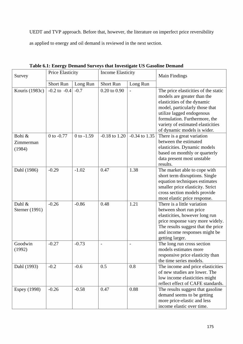
175
UEDT and TVP approach. Before that, however, the literature on imperfect price reversibility
as applied to energy and oil demand is reviewed in the next section.
Table 6.1: Energy Demand Surveys that Investigate US Gasoline Demand
Survey Price Elasticity Income Elasticity
Main Findings
Short Run Long Run Short Run Long Run Kouris (1983c) -0.2 to -0.4 -0.7 0.20 to 0.90 - The price elasticities of the static
models are greater than the elasticities of the dynamic model, particularly those that utilize lagged endogenous formulation. Furthermore, the variety of estimated elasticities of dynamic models is wider.
Bohi & Zimmerman (1984)
0 to -0.77 0 to -1.59 -0.18 to 1.20 -0.34 to 1.35 There is a great variation between the estimated elasticities. Dynamic models based on monthly or quarterly data present most unstable results.
Dahl (1986) -0.29 -1.02 0.47 1.38 The market able to cope with short term disruptions. Single equation techniques estimates smaller price elasticity. Strict cross section models provide most elastic price response.
Dahl & Sterner (1991)
-0.26 -0.86 0.48 1.21 There is a little variation between short run price elasticities, however long run price response vary more widely. The results suggest that the price and income responses might be getting larger.
Goodwin (1992)
-0.27 -0.73 - - The long run cross section models estimates more responsive price elasticity than the time series models.
Dahl (1993) -0.2 -0.6 0.5 0.8 The income and price elasticities of new studies are lower. The low income elasticities might reflect effect of CAFE standards.
Espey (1998) -0.26 -0.58 0.47 0.88 The results suggest that gasoline demand seems to be getting more price-elastic and less income elastic over time.

176
6.3.2 Imperfect Price Reversibility in Energy and Oil Demand Studies: Discussion of
Key Previous Papers
As discussed briefly and stated in Chapter 2, the imperfect price reversibility for gasoline
demand is reviewed in this section. The imperfect price reversibility concept for gasoline
demand has been investigated in a number of previous papers, such as Dargay (1992), Gately
(1992), Dargay and Gately (1995 and 1997), Gately and Streifel (1997), Gately and
Huntington (2002), Huntington (2006), and Huntington (2010). All of these studies
decomposed the price term (in logarithms) into three components, price maximum, price
recovery, and price cuts in order to estimate the differential asymmetric effects.56
Dargay (1992) investigated the asymmetric price responses by examining the demand for
motor fuels for road transport in France, Germany, and UK by using the annual data over the
period 1960 and 1988. She concluded that price shocks had a permanent effect that were not
reversible. According to Dargay (1992), in Germany the long run price elasticity is -0.44 and
demand does not respond to price falls; in France the long term price elasticity is -0.8 and
demand also reacts to price falls with an elasticity of -0.45; and in the UK the permanent
decline in demand is a result of a structural break caused by the price shocks in 1970s and all
other price rises and falls had negligible effects.
Gately (1992) investigated the imperfect price reversibility on US vehicle miles per driver,
miles per gallon and gasoline demand per driver by using the annual data over period 1966-
1989, 1966-1989 and 1960-1990 respectively. In all the cases, he rejects the perfect price
reversibility assumption; furthermore, the study illustrates that the gasoline demand response
56 The actual definition and calculation of price maximum, price recovery, and price cuts are explained later in the chapter.

177
to a new price maximum is approximately twice that of response to price cuts, whereas the
response to a price recovery is uncertain.
Dargay and Gately (1994) examined oil and energy demand for the OECD as a whole and the
regions within the OECD by utilizing the annual data over period 1970-1990. They
concluded that price reversibility is imperfect, with the impact of price increases larger than
the price decreases and the demand response for future income growth would not be
significantly smaller than in the past.
Dargay and Gately (1995) investigated the asymmetric price responses and income effect for
world energy and oil demand by using annual data over the period 1970-1991. They
concluded that demand in less developed countries is much more sensitive to income than the
demand in the industrialized countries. In industrialized countries, the price responses are
asymmetric, whereas in less developed countries there is less evidence for imperfect price
reversibility.
Dargay and Gately (1997) investigated the asymmetric price responses and income effect of
fuel demand for transport by using the pooled time series/cross section data over the period
1961-1990 for eleven OECD countries. They concluded that demand is not reversible to price
changes; response to price rises is greater than falling prices and price recoveries.
Gately and Streifel (1997) investigated the demand for oil products in 37 developing
countries with annual time series data over the period 1971-1993. Their results suggest that
income is the most significant driver of oil demand, and that oil exporting countries show
asymmetric responses to income increases and decreases. In only one third of the countries

178
that are investigated, the price of oil is found to be a significant factor and the estimated price
elasticities are smaller than the estimated income elasticities. Furthermore, the estimated
price responses of the countries differ; some petroleum products in some countries are found
to be symmetric and others asymmetric.
Gately and Huntington (2002) investigated the response of energy and oil demand to income
and price change for 96 of the world’s largest countries with annual time series data over the
period 1971 and 1997. They examined asymmetric price and income effects and the different
speed of adjustments to income and price variation. They concluded that the OECD demand
is more sensitive to price increases than to price decreases and not taking into account this
asymmetric effect can cause underestimated income elasticities. They also argue that the
demand response to income decline is not symmetric to its response to income increase for
most of the non-OECD countries and ignoring this asymmetric response can lead to biased
estimated income elasticities.
Griffin and Schulman (2005) criticizes Gately and Huntington (2002), arguing that the price
decomposition approach is really capturing exogenous energy saving technological progress,
which could be better characterized by a series of dummy variables for each year (given a
panel data approach is used). Their results for a panel of sixteen OECD countries over the
periods 1971 to 1996 and 1961 and 1999 suggest that asymmetric price terms are significant
is some cases for both energy and oil demand. However, the also find that the inclusion of
asymmetric price terms dramatically affects the income elasticity and conclude that
symmetric responses should be used for forecasting.

179
In his reply to Griffin and Schulman (2005), Huntington (2006) employs an F-Test in order to
evaluate the symmetric specification versus asymmetric specification and the inclusion or
exclusion of the time dummies. He found that for almost all the specifications for energy and
oil demand, symmetry was rejected at the 1% significance level and for the other
specification, symmetry was rejected at the 10% level of significance. He also found that that
the removal of the time dummies was rejected for all specifications at the 1% level of
significance. Hence, Huntington’s (2006) results suggest there might be a role for asymmetric
prices and a UEDT – an approach followed in the general model underpinning the research
for this chapter.57
Huntington (2010) investigated total oil, other petroleum products, gasoline, and residual fuel
oil demand for US over the period 1950 and 2005. He imposed both asymmetric price
responses and a deterministic trend and concluded that long term adjustments are greater than
short term adjustments and price increases higher than previous price hikes have a
significantly greater impact on long term energy demand.
In summary, these key studies suggest that oil and energy demand responds differently to
price increases above the previous maximum, price recoveries (below the previous
maximum) and price decreases and that this should be taken into account for policy
evaluation. The research for this chapter therefore incorporates asymmetric prices in the
general model to attempt to capture these effects within the STSM/UEDT framework as well
as allowing for TVPs. The next section therefore outlines the empirical framework used.
57 Although the UEDT in this chapter is in terms of a stochastic trend using time series data rather than times dummies used by Griffin and Schulman (2005) and Huntington (2006). Further support to incorporating both asymmetry and a UEDT for both time series and panel data is given in Adeyemi et al. (2010).
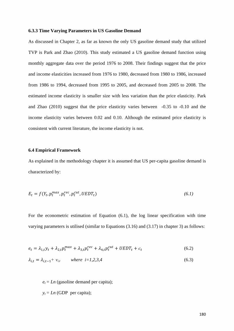
180
6.3.3 Time Varying Parameters in US Gasoline Demand
As discussed in Chapter 2, as far as known the only US gasoline demand study that utilized
TVP is Park and Zhao (2010). This study estimated a US gasoline demand function using
monthly aggregate data over the period 1976 to 2008. Their findings suggest that the price
and income elasticities increased from 1976 to 1980, decreased from 1980 to 1986, increased
from 1986 to 1994, decreased from 1995 to 2005, and decreased from 2005 to 2008. The
estimated income elasticity is smaller size with less variation than the price elasticity. Park
and Zhao (2010) suggest that the price elasticity varies between -0.35 to -0.10 and the
income elasticity varies between 0.02 and 0.10. Although the estimated price elasticity is
consistent with current literature, the income elasticity is not.
6.4 Empirical Framework
As explained in the methodology chapter it is assumed that US per-capita gasoline demand is
characterized by:
𝐸𝑡 = 𝑓(𝑌𝑡 , 𝑝𝑡𝑚𝑎𝑥, 𝑝𝑡
𝑟𝑒𝑐 , 𝑝𝑡𝑐𝑢𝑡 , 𝑈𝐸𝐷𝑇𝑡) (6.1)
For the econometric estimation of Equation (6.1), the log linear specification with time
varying parameters is utilised (similar to Equations (3.16) and (3.17) in chapter 3) as follows:
𝑒𝑡 = 𝜆1,𝑡𝑦𝑡 + 𝜆2,𝑡𝑝𝑡𝑚𝑎𝑥 + 𝜆3,𝑡𝑝𝑡
𝑟𝑒𝑐 + 𝜆4,𝑡𝑝𝑡𝑐𝑢𝑡 + 𝑈𝐸𝐷𝑇𝑡 + є𝑡 (6.2)
𝜆𝑖,𝑡 = 𝜆𝑖,𝑡−1+ νi,t where i=1,2,3,4 (6.3)
et = Ln (gasoline demand per capita);
yt = Ln (GDP per capita);

181
𝑝𝑡𝑚𝑎𝑥= cum. increase in the nat. log. of maximum historical real gasoline prices;
𝑝𝑡𝑟𝑒𝑐= cum. sub-maximum increase in the nat. log. of historical real gasoline prices;
𝑝𝑡𝑐𝑢𝑡= cum. decrease in the nat. log. of historical real gasoline prices in year t;
𝜆1,𝑡= the income elasticity at time t;
𝜆2,𝑡= price max elasticity at time t;
𝜆3,𝑡= price recovery elasticity at time t;
𝜆4,𝑡= price cut elasticity at time t;
𝑈𝐸𝐷𝑇𝑡= underlying energy demand trend for gasoline;
6.5 Data
US gasoline consumption and price data are obtained from the Energy Information Agency
(EIA, 2010c) Gross Domestic Product, the Consumer Price Index, and Population are
obtained from the US Department of Commerce Bureau of Economic Analysis (US BEA,
2010) for the period 1950 and 2008. In order to obtain the real gasoline price (P) and real
GDP (Y) the nominal prices and nominal GDP are deflated by the US Consumer Price Index
obtained from the US Department of Commerce Bureau of Economic Analysis (US BEA,
2010).
6.6 Estimation Results
In the first stage, the general specification with fixed coefficients as described in Equation
(3.17) in Chapter 3 is estimated and the following results are obtained for et� and illustrated in
Table 6.2.
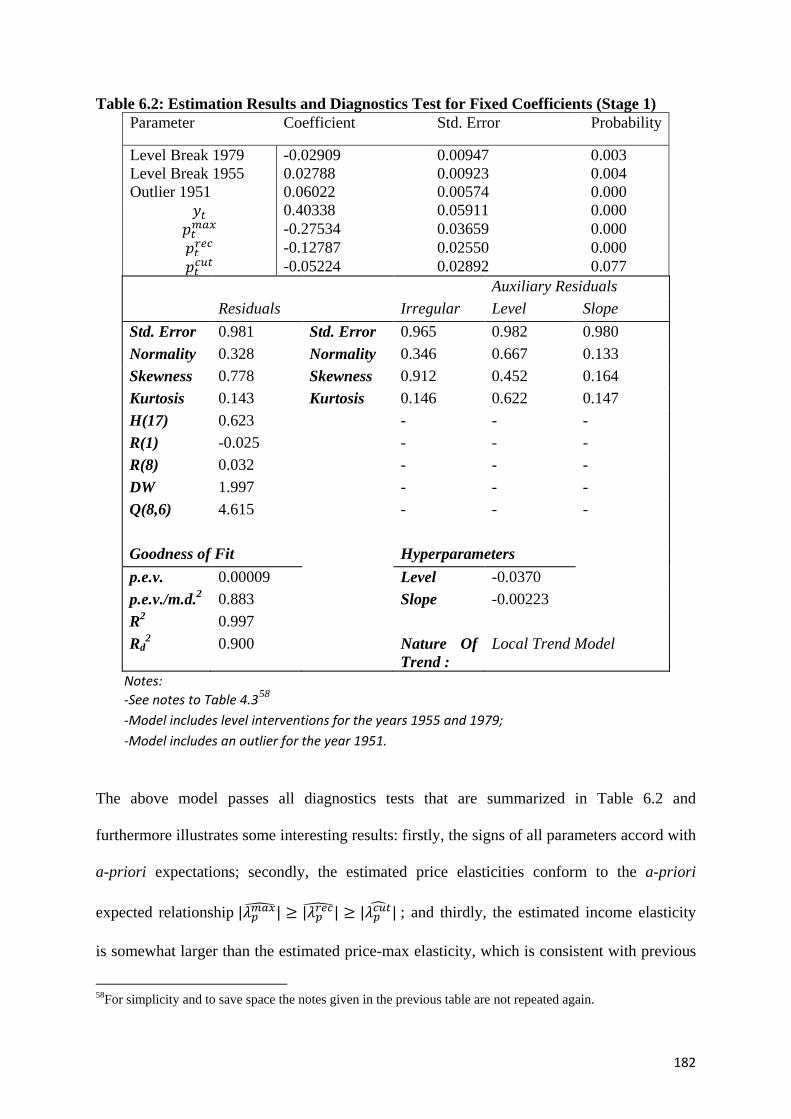
182
Table 6.2: Estimation Results and Diagnostics Test for Fixed Coefficients (Stage 1) Parameter Coefficient Std. Error Probability
Level Break 1979 -0.02909 0.00947 0.003 Level Break 1955 0.02788 0.00923 0.004 Outlier 1951 0.06022 0.00574 0.000
𝑦𝑡 0.40338 0.05911 0.000 𝑝𝑡
𝑚𝑎𝑥 -0.27534 0.03659 0.000 𝑝𝑡
𝑟𝑒𝑐 -0.12787 0.02550 0.000 𝑝𝑡
𝑐𝑢𝑡 -0.05224 0.02892 0.077 Auxiliary Residuals Residuals Irregular Level Slope Std. Error 0.981 Std. Error 0.965 0.982 0.980 Normality 0.328 Normality 0.346 0.667 0.133 Skewness 0.778 Skewness 0.912 0.452 0.164 Kurtosis 0.143 Kurtosis 0.146 0.622 0.147 H(17) 0.623 - - - R(1) -0.025 - - - R(8) 0.032 - - - DW 1.997 - - - Q(8,6) 4.615 - - - Goodness of Fit Hyperparameters p.e.v. 0.00009 Level -0.0370 p.e.v./m.d.2 0.883 Slope -0.00223 R2 0.997 Rd
2 0.900 Nature Of Trend :
Local Trend Model
Notes: -See notes to Table 4.358 -Model includes level interventions for the years 1955 and 1979; -Model includes an outlier for the year 1951.
The above model passes all diagnostics tests that are summarized in Table 6.2 and
furthermore illustrates some interesting results: firstly, the signs of all parameters accord with
a-priori expectations; secondly, the estimated price elasticities conform to the a-priori
expected relationship |𝜆𝑝𝑚𝑎𝑥� | ≥ |𝜆𝑝
𝑟𝑒𝑐� | ≥ |𝜆𝑝𝑐𝑢𝑡� | ; and thirdly, the estimated income elasticity
is somewhat larger than the estimated price-max elasticity, which is consistent with previous
58For simplicity and to save space the notes given in the previous table are not repeated again.
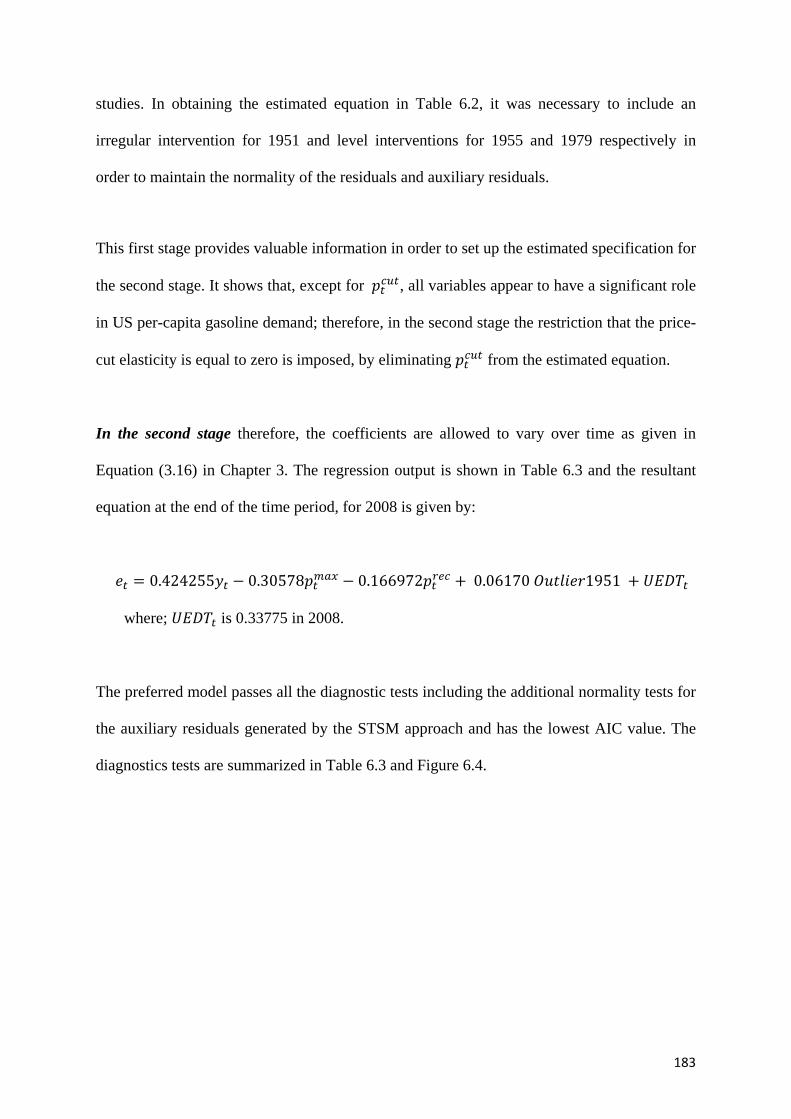
183
studies. In obtaining the estimated equation in Table 6.2, it was necessary to include an
irregular intervention for 1951 and level interventions for 1955 and 1979 respectively in
order to maintain the normality of the residuals and auxiliary residuals.
This first stage provides valuable information in order to set up the estimated specification for
the second stage. It shows that, except for 𝑝𝑡𝑐𝑢𝑡, all variables appear to have a significant role
in US per-capita gasoline demand; therefore, in the second stage the restriction that the price-
cut elasticity is equal to zero is imposed, by eliminating 𝑝𝑡𝑐𝑢𝑡 from the estimated equation.
In the second stage therefore, the coefficients are allowed to vary over time as given in
Equation (3.16) in Chapter 3. The regression output is shown in Table 6.3 and the resultant
equation at the end of the time period, for 2008 is given by:
𝑒𝑡 = 0.424255𝑦𝑡 − 0.30578𝑝𝑡𝑚𝑎𝑥 − 0.166972𝑝𝑡
𝑟𝑒𝑐 + 0.06170 𝑂𝑢𝑡𝑙𝑖𝑒𝑟1951 + 𝑈𝐸𝐷𝑇𝑡
where; 𝑈𝐸𝐷𝑇𝑡 is 0.33775 in 2008.
The preferred model passes all the diagnostic tests including the additional normality tests for
the auxiliary residuals generated by the STSM approach and has the lowest AIC value. The
diagnostics tests are summarized in Table 6.3 and Figure 6.4.

184
Table 6.3: Estimation Results and Diagnostics Test for TVP (Stage 2)
Parameter Coefficient Std.Error Probability Outlier 1951 0.06170 0.00706 0.000 Auxiliary Residuals Residuals Irregular Level Slope Std. Error 0.998 Std. Error 1.007 1.007 0.985 Normality 0.893 Normality 0.893 0.884 0.673 Skewness 0.803 Skewness 0.790 0.803 0.511 Kurtosis 0.667 Kurtosis 0.693 0.667 0.549 H(18) 0.692 - - - R(1) -0.061 - - - R(8) -0.084 - - - DW 2.103 - - - Q(8,6) 2.547 - - - Predictive Test 2001-2008 Information Criterion Akaike (AIC) Failure 0.8728 AIC(a) -8.9818 Cusum t(4) 1.5625 AIC(b) -8.9351 AIC(c) -5.4334 AIC(d) NA
Goodness of Fit Hyperparameters p.e.v. 0.0001 Level 0.3378 p.e.v./m.d.2 0.911 Slope 0.00218 R2 0.997 Rd
2 0.888 Nature Of Trend :
Local Trend Model
Notes: -See notes to Table 4.3 and Table 6.2. -Model includes an irregular for the year 1951; -Information Criterion Akaike compensates for the number of estimated parameters in the model so that comparing models, which has a different number of parameters become possible. Small AIC values indicate better fitting models. Normally, the model with the lowest AIC is the ‘statistically’ preferred model -AIC(a) represents model with time varying parameter and stochastic trend, AIC(b) represents model with fixed parameters and stochastic trend, AIC(c) represents model with fixed parameters and linear trend, and AIC(d) represents model with time varying parameters and linear trend (however, this model would not fully converge).
For the second stage, the resultant model has one irregular intervention for the year 1951. The
other interventions that were defined in the first stage (level interventions for 1955 and 1979)
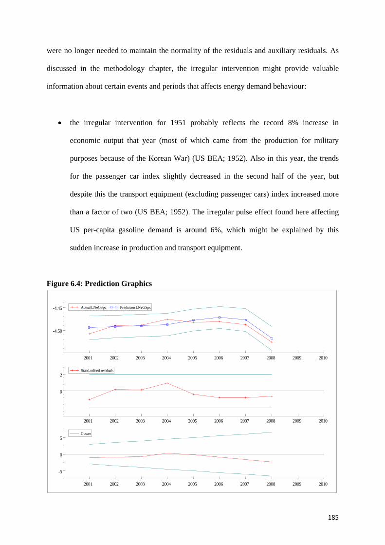
185
were no longer needed to maintain the normality of the residuals and auxiliary residuals. As
discussed in the methodology chapter, the irregular intervention might provide valuable
information about certain events and periods that affects energy demand behaviour:
• the irregular intervention for 1951 probably reflects the record 8% increase in
economic output that year (most of which came from the production for military
purposes because of the Korean War) (US BEA; 1952). Also in this year, the trends
for the passenger car index slightly decreased in the second half of the year, but
despite this the transport equipment (excluding passenger cars) index increased more
than a factor of two (US BEA; 1952). The irregular pulse effect found here affecting
US per-capita gasoline demand is around 6%, which might be explained by this
sudden increase in production and transport equipment.
Figure 6.4: Prediction Graphics
2001 2002 2003 2004 2005 2006 2007 2008 2009 2010
-4.50
-4.45 Actual LNeGSpc Prediction LNeGSpc
2001 2002 2003 2004 2005 2006 2007 2008 2009 2010
0
2Standardised residuals
2001 2002 2003 2004 2005 2006 2007 2008 2009 2010
-5
0
5Cusum

186
The historical movements of coefficients and the stochastic trend with its components (slope
and level) are presented in Figures 6.5 and 6.6 respectively. Although the elasticities vary
over time, these fluctuations are relatively very small (when reduced to two decimal places
they become identical). The estimated UEDT follows a stochastic process, which is
successfully captured by the STSM approach. The signs of all parameters accord with a-
priori expectations. Moreover; the estimated price elasticities have the following relationship
|𝜆𝑝𝑚𝑎𝑥� |>𝜆𝑝
𝑟𝑒𝑐� |>|𝜆𝑝𝑐𝑢𝑡� |61F
59which also accords with a-priori expectations, i.e. the estimated price-
max, price-recovery and price-cut elasticities are -0.31, -0.17 and 0 respectively. The
estimated income elasticity is 0.42, which is somewhat larger than the estimated price-max
elasticity and consistent with previous studies. These results are discussed in more detail in
the conclusion section below.
Figure 6.5: Time Varying Parameters
59𝜆𝑝
𝑐𝑢𝑡� being zero given it is insignificant and hence excluded from the preferred equation.
1950 1955 1960 1965 1970 1975 1980 1985 1990 1995 2000 2005 2010
0.4240
0.4245
Coefficient of GDP per capita
1950 1955 1960 1965 1970 1975 1980 1985 1990 1995 2000 2005 2010
-0.30578
-0.30578
Coefficient of Price max
1950 1955 1960 1965 1970 1975 1980 1985 1990 1995 2000 2005 2010
-0.16697
-0.16697
-0.16697Coefficient of Price recovery

187
Figure 6.6: UEDT of US Gasoline Demand and Slope-Level of UEDT
Given the preferred equation with the estimated non-linear UEDT has been obtained it is used
to construct future scenarios for US gasoline demand per capita. The next section therefore
outlines the assumptions about the future UEDT and other variables (price and income) that
are used to construct the scenarios and presents the forecast scenarios.
6.7 Forecast Assumptions
As in previous chapters, the three forecast scenarios are implemented, a ‘high’ case, a
‘reference’ case and a ‘low’ case. However, where data are available for 2009 and 2010
(including GDP per capita and gasoline prices)60 these are used in all scenarios. The detailed
information about these scenarios follows.
60 US GDP per capita decreased 4% in 2009 and increased 2% in 2010, whereas gasoline prices decreased 28% in 2009 and increased 17% in 2010 in real terms. Hence, the data for 2009 and 2010 are utilized for all scenarios.
1950 1955 1960 1965 1970 1975 1980 1985 1990 1995 2000 2005 2010
0.0
0.2
UEDT for US Gasoline Demand
1950 1955 1960 1965 1970 1975 1980 1985 1990 1995 2000 2005 2010
0.0
0.2
Level of UEDT
1950 1955 1960 1965 1970 1975 1980 1985 1990 1995 2000 2005 2010
0.00
0.02
Slope of UEDT

188
In the ‘reference’ scenario, it is assumed that real US gasoline price will increase by 1.5%
annually after 2010. The average annual prices increase is around 1% over the estimation
period however, the global oil demand is expected to increase at a faster pace in the future
because of increasing oil demand from emerging economies, therefore the price increase is
assumed slightly more than before. The increase in GDP per capita is expected to be 1% in
2011 and a 2% per annum thereafter. The average annual increase of GDP per capita is
around 2% over the estimation period; hence, it is assumed that after the recovery period
from the global economic crises GDP per capita will increase again by 2% annum. For the
UEDT, a slope of 0.00261 is projected for the period 2009-2020.
In the ‘low’ case scenario, it is assumed that the rise in the real US gasoline price will be
2.5% per annum after 2010, based on the assumption that the growing global demand for
gasoline will increase the gasoline prices faster than it has been observed before. For GDP it
is assumed that it will increase 0.5% in 2011 because of the economic recession and then
increase annually 1.5% per year (lower than the estimation period average) until 2020. For
the UEDT, a slope of -0.002 per annum between 2008 and 2020 is assumed suggesting that
US authorities will introduce policies aiming improvement in efficiency standards. A
graphical presentation of the scenario assumptions for GDP, real natural gas price index, and
the UEDT are illustrated in Figure 6.7.
In the ‘high’ case scenario, the real US gasoline price is assumed to increase 1% annually for
the period 2011-2020 (similar with the estimation period). Although it is expected that the
demand for oil from emerging economies will push the petroleum products price up, it is
assumed that although emerging technologies in the downstream will increase oil production,
61 Note that 0.002 is the same value of slope of UEDT at the end of estimation period.

189
this will balance the increase in demand. Furthermore, it is assumed that GDP will increase
2% in 2011 suggesting that US economy starts recovering from the global economic crisis,
followed by a slightly faster recovery period with an annual 2.5% increase for 2012, and will
increase by 3% per year thereafter to 2020. It is further assumed that energy using behaviour
will continue for US per-capita gasoline demand at an even greater pace, suggesting that US
citizens preference for the gasoline-fuelled appliances will increase faster than before. It is
therefore assumed that the UEDT has a slope of 0.004 over the forecast period.
Figure 6.7: Forecast Scenarios for Price, GDP per capita and UEDT
2000 2005 2010 2015 2020
40000
50000 GDP per capita (2000 constant US dollar) GDP per capita (Low)
GDP per capita (Ref) GDP per capita (High)
2000 2005 2010 2015 2020
1.5
2.0
2.5
3.0 Gasoline Price per Gallon (2000 constant US dollar) Price (Low)
Price (Ref) Price (High)
2000 2005 2010 2015 2020
0.30
0.35
0.40 UEDT UEDT (Low)
UEDT (Ref) UEDT (High)

190
6.8 Forecast Results
The three scenarios up to 2020 are illustrated in Figure 6.8. This shows that US per-capita
gasoline demand is projected to be 10, 11, and 12 barrels (1590, 1740, and 1908 litres) in
2020 according to the ‘low’, ‘reference’ and ‘high’ case scenarios respectively.
Figure 6.8: US Gasoline Demand per capita Forecast Scenarios
6.9 Summary and Conclusion
Environmental and energy security concerns have led policy makers to attempt to implement
measures in order to decrease US gasoline consumption. Carbon taxation is one of their
favoured measures given it is easy to implement relatively to alternatives. However, its
efficacy crucially depends on the price elasticity of gasoline demand, hence the importance of
acquiring sound and robust estimates of this vital parameter. Furthermore, it is important to
know how stable the estimate is; to have confidence that it is not going to change adversely
2000 2005 2010 2015 2020
9
10
11
12
13US Gasoline Demand per capita (Barrels) Low
Ref High

191
over time. Hence, it is vital that the most appropriate model is used to estimate these vital
parameters. It is argued here that the best way to achieve this is to estimate a US per capita
gasoline demand relationship using the STSM/UEDT approach with asymmetric price
responses in order to estimate the price and income elasticities as adopted in the research for
this chapter. Using annual data for the period 1949 and 2008, the results suggest the
following:
i) The fluctuations in the estimated income and price elasticities over the estimation
period are relatively small; in fact, when reduced to two decimal places they become
identical. Hence, these results suggest that they are stable over time.
ii) Price movements do not have a symmetric effect on US per-capita gasoline demand.
Changes in the maximum historical real gasoline prices have a greater impact on the
US gasoline demand than price recoveries that in turn has a greater impact than price
cuts, with the estimated elasticities of -0.31, -0.17, and zero respectively over the
estimation period.
iii) The estimated income elasticity is around 0.42 over the estimation period.
iv) The UEDT for US per-capita gasoline demand increases over the period 1949 to 1976
(except for 1952) and then starting from 1977 it declines until 1996 (except for 1994)
and starting from 1997 the direction of UEDT switches to being upward until 2008.
Between 1949 and 1976, the continuous increase in the underlying US per-capita
gasoline demand might be because of several factors such as, change in lifestyles and
widespread private car usage, and the rebound effect. After the first oil shock in 1973,
the Energy Policy and Conservation Act of 1975 established corporate average fuel
economy (CAFE) standards for new passenger cars. This act initiated the
manufacturing of more efficient cars and might well be a reason for the decline of the
UEDT between 1977 and 1996.

192
v) US per-capita gasoline demand is expected to be 10, 11, and 12 barrels by 2020,
according to the generated ‘low’, ‘reference’ and ‘high’ case scenarios.
The results of this chapter suggest that the asymmetric price responses should be taken into
account for sensible policy implications. US Congressional Budget Office (2008) used
symmetric price elasticity of -0.26 for their assessment of different policy options for
reduction of gasoline consumption and GHG emissions. However, the asymmetric price
responses might affect the policy makers decisions as the price elasticity of -0.26 and -0.17
might lead to different outcomes. The results of this chapter advocate that prices need to
increase above any previous maximum, otherwise the required demand reductions and GHG
savings will only be 1.7% instead of the 2.6% required.
Another important outcome of this research is that polices to try and drive down US gasoline
demand, other than raising prices through taxes, may have more of an impact given the
impact of the exogenous estimated UEDT. The estimated reductions that look to come
through exogenously via the UEDT appear (at times) to be driven by the CAFE standards,
suggesting that these have a noteworthy impact on reducing gasoline demand. Thus, the
imposition of even tighter CAFE standards should arguably be re-evaluated in the light of the
results found here.

193
CHAPTER 7: Summary and Conclusions
7.1 Introduction
The research for this thesis utilized the Structural Time Series Model (STSM) approach of
Harvey (1989) coupled with the Underlying Energy Demand Trend (UEDT) concept of Hunt
et al. (2003a and 2003b) to model and forecast:
i) Turkish Electricity demand (in Chapter 4);
ii) OECD-Europe natural gas demand (in Chapter 5); and
iii) US per-capita gasoline demand (in Chapter 6).
Chapter 1 discusses the importance of energy in our daily life and the factors that affect
energy demand as well as the importance of energy demand modelling. Chapter 1 also sets
out the objectives of the research and details the research questions that are attempted to be
answered. Chapter 2 presents the literature review, discussing the different energy demand
modelling approaches including arguing that in order to answer the research questions, an
econometric approach is chosen, in particular the STSM/UEDT approach which is adopted
throughout the research. Given this choice, Chapter 3 reviews previous energy demand
studies that have adopted a similar approach as well as explaining the STSM and the UEDT
concept in detail as well as the empirical framework, estimation strategy, and the way the
results are interpreted in Chapters 4-6. Chapter 3 also details how the future scenarios are
constructed in Chapters 4-6 as well explaining the extensions to the basic STSM/UEDT
approach introduced in Chapters 5 and 6.
The STSM/UEDT approach therefore underpins the research throughout the thesis since, as
argued in the earlier chapters, it is seen as the most appropriate econometric technique for
estimating energy demand relationships. Nonetheless, the core methodology was enhanced in

194
the latter chapters by attempting to analysis the relative importance of the economic and non-
economic drivers of OECD-Europe natural gas demand (Chapter 5) and including time
varying parameters and asymmetric price responses for US per-capita gasoline demand
(Chapter 6).
As explained in the introductory chapter, one of the main reasons for favouring the
STSM/UEDT approach is that, in addition, to estimating the impact of key economic drivers
of energy demand, income and price, it also attempts to capture the impact important, but
unobservable, components in a non-deterministic way. This thus allows for the identification
of important structural changes in energy demand behaviour, thus attempting to uncover
robust income and price elasticities. Information about points of structural change and robust
estimates of price and income elasticities of energy demand are vital for a number of energy
market participants (such as governments, regulative bodies, energy companies and financial
institutions) in order to assess the implications of past policy, to help reduce future
uncertainty, and to assist in developing future policy and its implications. Consequently, in
addition to the modelling and forecasting, the history of the energy situation and policies are
considered and evaluated, as well as offering some recommendations for where future energy
policy might develop for Turkish electricity (Chapter 4), OECD-Europe natural gas (Chapter
5), and US gasoline (Chapter 6).The next section therefore revisits and answers the Research
Questions outlined in Chapter 1 followed by the final section that summarizes the key policy
implications of the results and discuss the areas of possible future research.

195
7.2 Research Questions Re-visited
7.2.1 Main research questions
Q1: What are the advantages of STSM approach when estimating energy demand functions?
As discussed in detail, energy is a derived demand rather than being a demand for its own
sake and there are number of exogenous factors that affect the resultant energy demand.
Therefore, it is argued that it is important that these effects are not ignored when modelling
energy demand and attempting to estimate robust energy demand relationships. The uneven
structure of the exogenous factors makes it almost impossible to model them separately
and/or within a linear framework; hence, the need for the flexibility of the STSM/UEDT
approach to capture the effects adequately. The estimated UEDTs are important components
of energy demand reflecting how (holding price and income constant) energy demand
behaviour develops over time and it is argued that they should therefore be treated in an
appropriate way in order to obtain unbiased and robust elasticities and the STSM approach
provides a flexible framework to deal with the lumpiness characteristics of exogenous factors
that affect energy demand behaviour.
Q2: What are the implications of the estimated UEDTs, and the price and income elasticities
for future energy demand and policy analysis?
With the UEDTs estimated, the energy demand responses to income and price movements
are also estimated and it is argued that these estimates are more robust than alternative
estimates. Moreover, future projections are not just dependent upon income and price effects
but require thought and assumptions about future behaviour based upon the estimated
UEDTs over the past. Thus, future projections should also prove more robust as applied to
Turkish electricity, OECD-Europe natural gas and US per-capita gasoline (discussed further
below).

196
7.2.2 Sub Research Questions
In addition to the primary research questions, Chapter 1 introduced a number of sub-research
questions for the various sectors and fuels for Turkey, OECD-Europe, and the US:
-What are the shape and directions of UEDTs? Do they indicate any structural changes in
demand behaviour of the investigated countries?
-What is the best estimate of short-long run price and income elasticities?
-What will be the future energy demand?
In addition, the following sub research question was introduced for OECD-Europe natural
gas demand:
-What are the relative contributions of income, price, and the UEDT in driving OECD-
Europe natural gas demand?
Finally, the following two additional sub research questions were in included for US per
capita gasoline demand:
-Are Asymmetric Price Responses important in driving US gasoline demand per capita?
-Is there evidence of time varying elasticities for US gasoline demand per capita?

197
The answers for these sub questions are as follows:
i) For the Turkish Industrial Sector
- The estimated UEDT is generally increasing (but at a decreasing rate) over the
estimation period, i.e. it is generally energy using; as shown in Figure 7.1. The
estimated UEDT for the Turkish industrial sector is generally increasing, but the
underlying rate of increase diminishes with a significant structural change in 1981
(reflecting the implementation of the first planned energy conservation activities by
the General Directorate of Electrical Power Resources Survey Administration-EIE).
Figure 7.1: Underlying Electricity Demand Trend (UEDT) of Turkish Industrial Sector Electricity Consumption 1960-2008
-The estimated industrial value added (output) elasticity is 0.15 and the estimated
industrial energy price elasticity is -0.16.
- Turkish industrial is projected to be 97, 121, and 148 TWh by 2020 according to the
‘low’, ‘reference’ and ‘high’ case scenarios respectively.
1960 1965 1970 1975 1980 1985 1990 1995 2000 2005 2010
17.5
18.0
18.5
19.0
19.5
20.0
20.5
lnUEDT for Turkish Industrial Electricity Consumption
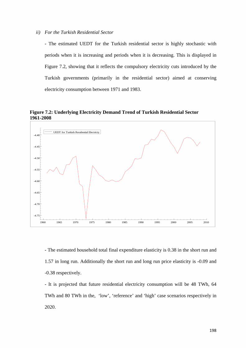
198
ii) For the Turkish Residential Sector
- The estimated UEDT for the Turkish residential sector is highly stochastic with
periods when it is increasing and periods when it is decreasing. This is displayed in
Figure 7.2, showing that it reflects the compulsory electricity cuts introduced by the
Turkish governments (primarily in the residential sector) aimed at conserving
electricity consumption between 1971 and 1983.
Figure 7.2: Underlying Electricity Demand Trend of Turkish Residential Sector 1961-2008
- The estimated household total final expenditure elasticity is 0.38 in the short run and
1.57 in long run. Additionally the short run and long run price elasticity is -0.09 and
-0.38 respectively.
- It is projected that future residential electricity consumption will be 48 TWh, 64
TWh and 80 TWh in the, ‘low’, ‘reference’ and ‘high’ case scenarios respectively in
2020.
1960 1965 1970 1975 1980 1985 1990 1995 2000 2005 2010
-4.75
-4.70
-4.65
-4.60
-4.55
-4.50
-4.45
-4.40UEDT for Turkish Residential Electricty

199
iii) For Turkish Aggregate Electricity Demand:
- The estimated UEDT for the Turkish aggregate electricity is generally upward
sloping (energy using) but at a generally decreasing rate as shown in Figure 7.3.
- The estimated income and price elasticities for Turkish aggregate electricity are 0.17
and -0.11 respectively.
Figure 7.3: Underlying Aggregate Electricity Demand Trend of Turkey 1960-2006
-Turkish aggregate electricity consumption is predicted to be 259, 310, and 368 TWh
in the ‘low’, ‘reference’ and ‘high’ case scenarios respectively by 2020.
iv) For OECD-Europe Natural Gas Demand:
-The estimated UEDT for OECD-Europe natural gas demand is increasing and
decreasing over the estimation period but generally decreasing after 1996 as displayed
in Figure 7.4.
1960 1965 1970 1975 1980 1985 1990 1995 2000 2005 2010
17.5
18.0
18.5
19.0
19.5
20.0
20.5
21.0UEDT for Turkish Total Electricity Demand

200
Figure 7.4: The estimated UEDT of Natural Gas Demand of OECD Europe 1972-2008
- The estimated short and long run GDP and price elasticities for OECD-Europe
natural gas demand are 0.95 and -0.18 respectively
-The OECD-Europe natural gas demand is expected to be 295, 357 and 468 mtoe by
2020, according to the generated low, reference and high case scenarios.
-The relative contributions of income, price and the UEDT in driving OECD-Europe
natural gas demand is shown in Figure 7.5. This shows that the estimated contribution
from income is consistently high, suggesting it was and remains the main driver of
OECD-Europe natural gas demand. Whereas the estimated contribution from the
UEDT has periods when it was relative important and periods when it was not but, in
contrast, the estimated contribution from price is relatively small.
1980 1985 1990 1995 2000 2005
4.44
4.46
4.48
4.50
4.52
4.54
4.56
Ln
UEDT

201
Figure 7.5: Estimated Contributions to the Annual Percentage Change in OECD-Europe Natural Gas Demand
v) For US Per Capita Gasoline Demand:
- The estimated UEDT for US per capita gasoline demand increases over the period
1949 to 1976 (except for 1952) and then starting from 1977 it declines until 1996
(except for 1994) and starting from 1997 the direction of UEDT switches to being
upward until 2008, as shown in Figure 7.5. Between 1949 and 1976 the continuous
increase of in underlying US per-capita gasoline demand (holding income and price
constant) reflects several factors such as, change in life styles and widespread of
private car usage, and the rebound effect. Furthermore, it reflects that after the first oil
shock in 1973, the Energy Policy and Conservation Act of 1975 established corporate
average fuel economy (CAFE) standards for new passenger cars. This act, which
initiated the manufacturing of more efficient cars (Greene, 1990), is reflected in the
decline of the estimated UEDT between 1977 and 1996.
0%
10%
20%
30%
40%
50%
60%
70%
80%
90%
100% 19
80
1981
19
82
1983
19
84
1985
19
86
1987
19
88
1989
19
90
1991
19
92
1993
19
94
1995
19
96
1997
19
98
1999
20
00
2001
20
02
2003
20
04
2005
20
06
2007
20
08
2009
Share of Income Contribution Share of Price Contribution Share of UEDT Contribution

202
Figure 7.6: UEDT of US Gasoline Demand and Slope-Level of UEDT
- Price movements do not affect US gasoline demand symmetrically. Changes in the
maximum historical real gasoline prices have a greater impact on the US gasoline
demand than price recoveries that in turn has a greater impact than price cuts, with the
estimated elasticities of -0.31, -0.17, and zero respectively over the estimation period.
The estimated income elasticity is around 0.42 over the estimation period 1949 to
2008. Furthermore, there is no evidence that income and price elasticities vary over
time.
-It is projected that US per capita gasoline demand will be 10, 11, and 12 barrels
(1590, 1740, and 1908 litres) by 2020, according to the generated low, reference and
high case scenarios.
1950 1955 1960 1965 1970 1975 1980 1985 1990 1995 2000 2005 2010
-0.10
-0.05
0.00
0.05
0.10
0.15
0.20
0.25
0.30
0.35UEDT for U.S. Gasoline Demand

203
7.3 Conclusion and Future Research Areas
The energy needs of modern societies are currently mostly met by exhaustible fossil fuels.
Energy scarcity is one of the important obstacles for sustainable economic growth. During the
1980s and 1990s, because of the relatively low and stable energy prices, the interest for
energy demand studies diminished. However, in today’s world the rapid increase in energy
demand mostly coming from emerging economies has triggered concerns about energy
scarcity and security. Different to the past, energy prices have (and are likely to continue to)
go beyond their historical peaks and the need for rational planning might well become a
priority for nations whose economic growth is highly dependent on energy. The
understanding of energy consuming behaviour and robust reliable future projections of
energy demand has therefore arguably never been so vital for welfare of humankind (Slade et
al. 1993).
Therefore, this thesis, and the research that underpins it, demonstrates the advantages of the
STSM coupled with the UEDT concept when estimating energy demand models, in addition
to showing how it can be augmented with asymmetric price responses and time varying
parameters. It is argued that the STSM approach has significant advantages in terms of:
• modelling stochastic UEDTs with its flexible empirical framework;
• identifying unbiased and robust price and income elasticities by taking into
account the UEDT; and
• identifying structural breaks and changes in energy demand behaviour.
Therefore, the STSM approach enables the estimation of robust energy demand models that
are vital for policy makers and other market participants. Firstly, they arguably enable the
generation of better projections thus allowing the development of better policy tools and

204
measures for future energy demand policy. Secondly, by detecting the structural changes in
the UEDTs, the STSM allows an assessment of the impacts of past policy decisions on
energy demand behaviour; hence, using this approach arguably facilitates the choice of the
more effective policies. Finally, by providing information about the components of the UEDT
(such as the level and the slope), the STSM provides information about the unobserved
components that affect energy demand behaviour; thus making it possible to develop
assumptions about our future expectations of these unobserved components.
That said, there is still scope to improve the research. Further research could disaggregate the
Turkish sectors further to analyse sub industries in order to better understand their energy
consuming behaviour and provide a more disaggregated forecast. Similarly, OECD-Europe
gas demand could be disaggregated into to smaller regions and/or countries to test the
robustness of the results and projections found here. Moreover, although the time varying
parameters approach applied in Chapter 6 did not provide any evidence that income and price
elasticities change over time, this might not always be the case. Hence, future energy demand
models might explore this approach with general models assuming that the parameters do
vary over time and only accepting that the elasticities are constant over time if that is
accepted by the data – and the STSM approach has power to estimate such models. And one
final point, although it has been argued that the STSM has a important advantage in terms of
estimating a stochastic trend, an interesting extension to this research would be to compare
the outcome here with more conventional econometric approaches, such as VECM type
models of energy demand in order to evaluate the performance of different empirical
frameworks.

205
Despite these possible extensions and improvements, this thesis has addressed a number of
major issues in the energy demand modelling literature, combining and exploring several of
them to examine different types of energy demands for different countries or group of
countries. The insights, results and projections provided by this research should be of
particular value to policy makers helping to reduce the risks related with the uncertainty of
future energy demand and aid long term energy planning activities.
206
Bibliography
1. Adeyemi OI and Hunt LC. 2007. “Modelling OECD Industrial Energy Demand: Asymmetric Price Responses and Energy Saving Technical Change.” Energy Economics, 29; pp. 693-709.
2. Adeyemi OI, Broadstock DC, Chitnis M, Hunt LC and Judge G. 2010. “Asymmetric price responses and the underlying energy demand trend: Are they substitutes or complements? Evidence from modelling OECD aggregate Energy Demand.” Energy Economics, 32; pp. 1157-1164.
3. Agnolucci P. 2009. “Stochastic Trends and Technical Change: The Case of Energy Consumption in the British Industrial and Domestic Sectors.” The Energy Journal; 31, pp. 111-135.
4. Akay D and Atak M. 2006. “Grey Prediction with Rolling Mechanism for Electricity Demand Forecasting of Turkey.” Energy; 32: pp. 1670-1675.
5. Altas M, Fikret H and Celebi E. 1994. “6th Turkish Energy Congress, Energy Statistics.” 17-22 October 1994 Izmir, Turkey (in Turkish).
6. Altinay G and Karagol E. 2005. “Electricity Consumption and Economic Growth: Evidence from Turkey.” Energy Economics; 27; pp. 849-856.
7. Amarawickrama HA and Hunt LC. 2008. “Electricity Demand for Sri Lanka: A Time Series Analysis.” Energy; 33; pp. 724-739.
8. Arbex, MA and Perobelli FS. 2010. “Solow meets Leontief: Economic Growth and Energy Consumption.” Energy Economics; 32 (1); pp. 43-53.
9. Asteriou D and Hall SG. 2006. “Applied Econometrics” Palgrave Macmillan, New York, US.
10. Bakirtas T, Karbuz S and Bildirici M. 2000. “An Econometric Analysis of Electricity Demand in Turkey. Middle East Technical University, METU Studies in Development; 27/1-2; pp. 23-34 Ankara Turkey.
11. Beenstock M and Willcocks P. 1983. “Energy and Economic activity: A Reply to Kouris.” Energy Economics; 5; pp. 212.
12. Beenstock M and Willcocks P. 1981.” Energy Consumption and Economic Activity in Industrialized countries.” Energy Economics; 3; pp. 225-232.
13. Bhattacharya SC. 2011. “Energy Economics: Concepts, Issues, Market and Governance” Springer, London, UK.
14. Bhattacharyya SC and Timilsina GR. 2009. “Energy Demand Models for Policy Formulation: A Comparative Study of Energy Demand Models” The World Bank Development Research Group Environment and Energy Team, Policy Research Working Paper No: 4866.
15. Bilgin M. 2009. “Geopolitics of European natural gas demand: Supplies from Russia, Caspian and Middle East.” Energy Policy; 37; pp. 4482-4492.

207
16. Bohi DR. 1981. Analyzing Demand Behaviour: A Study of Energy Elasticities. John Hopkins University Press: Baltimore, US.
17. Bohi DR and Zimmerman MB. 1984. “An Update on Econometric Studies of Energy Demand Behaviour.” Annual Review of Energy; 9; pp. 105-154.
18. Box GPE and Jenkins GM. 1976. “Time Series Analysis: Forecasting and Control” Revised edition, Holden Day, San Francisco, US.
19. British Petroleum (BP).2005. Statistical Review of World Energy.
20. Broadstock DC and Hunt LC. 2010. “Quantifying the Impact of Exogenous Non-Economic Factors on UK Transport Oil Demand.” Energy Policy; 38; pp. 1559-1565.
21. Brown JP, Song H and McGillivray A. 1997. “Forecasting UK House Prices: A Time Varying Coefficient Approach.” Economic Modelling; 14; pp. 529-548.
22. Ceylan H, Ozturk HK. 2004. “Estimating energy demand of Turkey based on economic indicators using genetic algorithm approach.” Energy Conversion and Management; 45; pp. 2525-2537.
23. Chateau B and Lapillonne B.1978. “Long term energy demand forecasting: A new approach” Energy Policy; 62(2); pp. 140-157.
24. Chitnis M and Hunt LC. 2011. “Modelling UK household expenditure: economic versus noneconomic drivers” Applied Economics Letters; 18(8); pp. 753-767.
25. Chitnis M and Hunt LC. 2012. “What drives the change in UK household energy expenditure and associated CO2 emissions? Implication and forecast to 2020.” Applied Energy; 94; pp. 202-214.
26. Christoffersen G. 1998. “China’s Intentions for Russian and Central Asian Oil and Gas.” The National Bureau of Asian Research; Vol:9, 2.
27. Codoni R, Park HC and Ramani KV. 1985. “Integrated Energy Planning –A Manual” Asia Pacific Development Centre, Kuala Lumpur.
28. Commandeur JF and Koopman SJ. 2007. “An Introduction to State Space Time Series Analysis.” Oxford University Press: Oxford, UK.
29. Common MS .1981. “Implied Elasticities in Some UK Energy Projections.” Energy Economics; 3; pp. 153-158.
30. Dahl C and Sterner T. 1991. “A survey of econometric gasoline demand elasticities.” International Journal of Energy Systems; 11; pp. 53-76.
31. Dahl C. 1986. “Gasoline Demand Survey.” The Energy Journal; 7; pp. 67-82.
32. Dahl C. 1993. “A Survey of Energy Demand Elasticities in Support of Development of the NEMS.” US Department of Energy, US.
33. Dargay JM and Gately D. 1994. “Oil Demand in the Industrialized Countries.” Energy Journal; 15; pp. 39-67.

208
34. Dargay JM and Gately D. 1997. “The Demand for Transportation Fuels: Imperfect Price Reversibility?” Transportation Research Part-B; 31 (1); pp.71-82.
35. Dargay, JM. and Gately D.1995. “The Response of World Energy and Oil Demand to Income Growth and Changes in Oil Prices.” Annual Review of Energy; 20, pp. 145–178.
36. Dargay JM. 1992. “The Irreversible Effects of High Oil Prices: Empirical Evidence for the Demand for Motor Fuels in France, Germany, and the UK.” in Energy Demand: Evidence and Expectations, ed. D. Hawdon, pp. 165-82. Academic Press London, UK.
37. Denison M. 2009. “The EU and Central Asia: Commercialising the Energy Relationship.” EU-Central Asia Monitoring Working Paper, 2. Retrieved on 24 February 2011 from http://www.ceps.eu/files/book/1883.pdf on 24 February 2011.
38. Deutche Welle, 2009. “Proposed Nabucco Pipeline gets European Bank Backing.” Retrieved on 30 March 2010 from http://www.dw-world.de/dw/article/0,,3980038,00.html
39. Dickey A and Fuller WA. 1979. “Distribution of the Estimators for Autoregressive Time Series with a Unit Root.” Journal of the American Statistical Association; Vol. 74 No 366pp. 427-431.
40. Dimitropoulos J, Hunt LC and Judge G. 2005. “Estimating Underlying Energy Demand Trends using UK Annual Data.” Applied Economics Letters; 12 (4); pp. 239-244.
41. Dolun L. 2002. “The Power Generation in Turkey and the Resources.” Turkish Development Bank, Research Report, Ankara. (in Turkish translated by author) http://www.kalkinma.com.tr/data/file/raporlar/ESA/SA/2002-SA/SA-02-06-18_Elektrik_Enerjisi_Sektoru.pdf
42. Doornat V, Koopman SJ, Ooms M, Dessertaine A and Collet J. 2008. “An Hourly Periodic State Space Model for Modelling French National Electricity Load.” International Journal of Forecasting; 24; pp. 566-587.
43. Ediger V and Akar S. 2007. “ARIMA Forecasting of Primary Energy Demand by Fuel in Turkey.” Energy Policy; 35;pp. 1701-1708.
44. Ediger V and Tatlidil H.2002. “Forecasting the Primary Energy Demand in Turkey and Analysis of Cyclic Patterns.” Energy Conversion and Management; 43; pp. 473-487.
45. Engel RF and Granger CWJ. 1987. “Co-integration and Error-correction: Representation, Estimation and Testing.” Econometrica; 55; pp. 251-76.
46. Epsey M. 1998. “Gasoline Demand Revisited: An International Meta-Analysis of Elasticities.” Energy Economics; 20; pp. 273-295.
47. Erbaykal E. 2008. “Disaggregate Energy Consumption and Economic Growth: Evidence from Turkey.” International Research Journal of Finance and Economics; 20 ;pp. 172-179.

209
48. Erdal G, Erdal H and Esengun K. 2008. “The causality between energy consumption and economic growth in Turkey.” Energy Policy; 36; pp. 3838-3842.
49. Erdogdu E. 2007. “Electricity Demand Analysis Using Co-integration and ARIMA Modelling: A Case Study of Turkey.” Energy Policy; 35; pp. 1129-1146.
50. Estrada J and Fugleberg O. 1989. “Price elasticities of natural gas demand in France and West Germany.” The Energy Journal; 10; pp. 77-90.
51. Eurogas, 2007. “Natural gas demand and supply long term outlook to 2030.” Eurogas. Retrieved on 5 March 2010 from http://www.eurogas.org/figures_statistics.aspx on 05 March 2010.
52. European Commission, 2009. “The January 2009 Gas Supply Disruption to the EU: An Assessment.” Commission Staff Working Document Accompanying Document SEC 977. Retrieved on 11 February 2011 from http://ec.europa.eu/energy/strategies/2009/doc/sec_2009_0977.pdf.
53. Foreign and Commonwealth Office-FCO. 2010. “Turkey : Country Profile”. Retrieved on 14 August 2010 from http://www.fco.gov.uk/en/travel-and-living-abroad/travel-advice-by-country/country-profile/europe/turkey/?profile=today.
54. Gately D. 1992. “Imperfect Price-Reversibility of US Gasoline Demand: Asymmetric Responses to Price Increases and Decreases.” Energy Journal; 13 pp. 412-435.
55. Gately D. Huntington HG. 2002. “The Asymmetric Effects of Changes in Price and Income on Energy and Oil Demand.” The Energy Journal; 23, pp. 19-55.
56. Gately D. Streifel SS. 1997. “The Demand for Oil Products in Developing Countries.” World Bank Discussion Paper No: 359.
57. Goodwin PB. 1992. “A review of new demand elasticities with special reference to short and long run effects of price changes.” Journal of Transport Economics and Policy; 2, pp. 155-169.
58. Granger CW and Newbold P. 1974. “Spurious regressions in econometrics.” Journal of Econometrics; 2, pp. 111-120.
59. Greene D. 1990. “CAFE or Price? : An Analysis of the Effects of Federal Fuel Economy Regulations and Gasoline Price on New Car MPG, 1978-89” The Energy Journal; 11(3); pp. 37-58.
60. Griffin JM, Schulman CT. 2005. “Price Asymmetry in Energy Demand Models: A Proxy for Energy Saving Technical Change.” The Energy Journal; 26 (2); pp. 1–21.
61. Griffin JM. 1979. “Energy conservation in OECD: 1980-2000.” Ballinger Publishing Company Cambridge, UK.
62. Haas R, Schipper L. 1998. “Residential Energy Demand in OECD- Countries and the Role of Irreversible Efficiency Improvements.” Energy Economics; 20; pp. 421-442.
210
63. Halicioglu F. 2007. “Residential Electricity Demand Dynamics in Turkey.” Energy Economics; 29; pp. 199-210.
64. Hall G and Grant T. 2009. “Russia, China and Energy Security Politics of the Caspian Region after Cold War.” Mediterranean Quarterly; 2; pp. 113-137.
65. Hamzacebi C. 2007. “Forecasting of Turkey’s net electricity consumption on sectoral bases.” Energy Policy; 35; pp. 2009-2016.
66. Hanfer M Karbuz S and Andaloussi HE. 2009. “Long Term Natural Gas Supply to Europe: Import Potential, Infrastructure Needs and Investment Promotion.” Energy and Environment; 19- 8; pp. 1131-1153.
67. Hartman RS. 1979. “Frontiers in Energy Demand Modelling.” Annual Review of Energy; 4; pp. 433-466.
68. Harvey AC and Koopman SJ. 1993. “Forecasting hourly electricity demand using time varying splines.” Journal of American Statistical Association; 88-424; pp. 1228-1236.
69. Harvey AC and Scott A. 1994. “Seasonality in dynamic regression models.” Economic Journal; 104; pp. 1324–1345.
70. Harvey AC and Shephard N. 1993. “Structural Time Series Models.” In: Maddala GS, Rao CR and Vinod HD (Eds), Handbook of Statistics, Vol. 11 North Holland: Amsterdam; pp. 261-302.
71. Harvey AC, and Koopman SJ. 1993. “Forecasting Hourly Electricity Demand Using Time Varying Splines.” Journal of American Statistical Association 88-424; pp. 1228-1236.
72. Harvey AC, Henry SGB, Peters S and Wren-Lewis S. 1986. “Stochastic Trends in Dynamic Regression Models: An Application to the Employment–output Equation.” Economic Journal; 96; pp. 975–985.
73. Harvey AC, Koopman SJ and Shephard N. 2005."State Space and Unobserved Component Models: Theory and Applications.” Cambridge University Press: Cambridge, UK.
74. Harvey AC. 1989. “Forecasting, Structural Time Series Models and the Kalman Filter.” Cambridge University Press, Cambridge, UK.
75. Harvey AC. 1997. “Trends, cycles and auto regressions.” Economic Journal; 107; pp. 192–201.
76. Helen H. 2010. “The EU’s Energy Security Dilemma with Russia.” POLIS Journal; Vol. 4.
77. Hepbasli A and Ozalp N. 2003. “Development of energy efficiency and management implementation in the Turkish industrial sector.” Energy Conversion and Management; 44, pp. 231-249.
78. Holz F, Hirschhausen C and Kemfert C. 2006. “A Strategic Model of European Gas Supply (GASMOD).” German Institute for Economic Research. Berlin, Germany.
211
79. Honore A. 2006. “Future Natural Gas Demand in Europe: The Importance of the Power Sector.” Oxford Institute for Energy Studies, Oxford, UK.
80. Houthhakker HS. 1951. “Some calculations of electricity consumption in Great Britain.” Journal of Royal Statistical Society; 114; pp. 351-371.
81. Hunt LC and Manning N. 1989. “Energy Price and Income Elasticities of Demand: Some Estimates for the UK Using the Co-integration Procedure.” Scottish Journal of Political Economy; 36(2); pp. 183-193.
82. Hunt LC and Ninomiya Y. 2003. “Unravelling Trends and Seasonality: A structural Time Series Analysis of Transport Oil Demand in the UK and Japan.” The Energy Journal; 24-3; pp. 63-69.
83. Hunt LC, Judge G and Ninomiya Y. 2000. “Modelling Technical Progress: An Application of the Stochastic Trend Model to UK Energy Demand.” Surrey Energy Economics Discussion Paper SEEDS No. 99.
84. Hunt LC, Judge G. and Ninomiya Y. 2003a. “Modelling Underlying Energy Demand Trends.” in Energy in Competitive Market: Essays in Honour of Colin Robinson pp. 140-174. Hunt LC (Ed) Edward Elgar, UK .
85. Hunt LC, Judge G. and Ninomiya Y. 2003b “Underlying Trends and Seasonality in UK Energy Demand: A Sectoral Analysis.” Energy Economics 2003b; 25; pp. 93–118.
86. Huntington H. 2006. “A Note on Price Asymmetry as Induced Technical Change.” Energy Journal; 27; pp. 1–7.
87. Huntington HG. 2010. “Short and Long Run Adjustments in US Petroleum Consumption. Short- and Long-Run Adjustments in US Petroleum Consumption.” Energy Economics; 32; pp. 63-72.
88. IEA: International Energy Agency, 2011. Energy Balances for OECD Countries. Retrieved on 08 January 2011 from http://esdsw1.mc.manchester.ac.uk/WDS_IEA/TableViewer/tableView.aspx?ReportId=960.
89. IEA: International Energy Agency. 2010a. “CO2 Emissions from Fuel Combustion -2010.” International Energy Agency, France.
90. IEA: International Energy Agency. 2010b. “World Energy Outlook-2010.” International Energy Agency, France.
91. IEA: International Energy Agency, 2010c. Energy Balances for OECD Countries. Retrieved on 08 January 2009 from http://esdsw1.mc.manchester.ac.uk/WDS_IEA/TableViewer/tableView.aspx?ReportId=960.
92. IEA: International Energy Agency. 2010d. “Natural Gas Information-2010.” International Energy Agency, France.
93. IEA: International Energy Agency. 2008. “World Energy Outlook-2008.” International Energy Agency, France.

212
94. International Energy Agency-IEA. 2005. “Energy Policies of IEA Countries Turkey 2005 Review.” IEA publications, Paris, France.
95. International Monetary Fund-IMF. 2005. “Will the oil market continue to be tight?” Chapter IV of World Economic Outlook”. Retrieved on 1 February 2010 from https://www.imf.org/external/pubs/ft/weo/2005/01/pdf/chapter4.pdf.
96. Jalles JT. 2009. “Structural Time Series Model and the Kalman Filter: A Concise Review.” FEUNL Working Paper Series wp 541.
97. Jobert T and Karanfil F. 2007. “Sectoral energy consumption by source and economic growth in Turkey.” Energy Policy ; 35; pp. 5447-5456.
98. Johansen S. 1988. “Statistical Analysis of Co-integrating Vectors” Journal of Economic Dynamics and Control; 12; pp. 231-254.
99. Johansen S. 1991. “Estimating and Hypothesis Testing of Co-integrating Vector Autoregressive Models” Econometrica; 59; pp. 1551-1589.
100. Johansen S. and Juselius K. 1990.“Maximum likelihood estimation and inference on co-integration with applications to the demand for money”, Oxford Bulletin of Economics and Statistics; 52(2); pp. 169-210.
101. Kalman RE. 1960. “A New Approach to Linear Filtering and Prediction Problems.” Journal of Basic Engineering; 82; pp. 35-45.
102. Karanfil F. 2008. “Energy Consumption and Economic Growth Revisited: Does the Size of Unrecorded Economy Matter?” Energy Policy; 36; pp. 3029-3035.
103. Kavaklioglu K, Ceylan H, Ozturk HK and Canyurt OE. 2009. “Modelling and Prediction of Turkey’s Electricity Consumption Using Artificial Neural Networks.” Energy Conservation and Management; 50; pp. 2719-2727.
104. Kavalov B, Petric H and Georgakaki A. 2009. “Liquefied Natural Gas for Europe : Some important issues for consideration.” European Commission Joint Research Centre Reference Reports. Netherlands.
105. Kazgan G. 2002. “The Economic Crises in Turkey (1929-2001): A comparison of causes and the results.” (in Turkish translated by author). Retrieved on 05 march 2009 from http://kazgan.bilgi.edu.tr/main.asp?p=makaleler.
106. Keleş SM. 2005. “Electricity demand forecasts and their effects on Turkish economy. (In Turkish translated by author) Republic of Turkey Prime Ministry under Secretariat of Treasury Ankara. Retrieved on 14 March 2009 from http://www.hazder.org.tr/tezler/ Mehmet_Sertac_Keles-Elektrik_Enerjisi_Talep_Tahminleri_ve_Turkiye_ Ekonomisine_Etkileri.pdf.
107. Kim CJ. 1993. “Sources of Monetary Growth Uncertainty and Economic Activity: Time Varying Parameter Model with Heteroskedastic Disturbances.” The Review of Economics and Statistics; 75; pp. 483-492.
108. Kirby SN.1983. “Residential Demand for Energy: A Review of the Empirical Literature and Some New Results.” Rand Corporation, Santa Monica, US.

213
109. Koopman SJ, Harvey AC, Doornik JA and Shephard N. 2007. STAMP Version 8 Econometric Software International Timberlake Consultants, London, UK.
110. Kouris, G. 1983a. “Energy Consumption and Economic Activity in Industrialised Economies: A note” Energy Economics; 17; (2), pp. 133 – 143.
111. Kouris G. 1983b. “Fuel Consumption and Economic Activity in Industrialised Economies: A Note.” Energy Economics; 5;pp. 207-212.
112. Kouris, G. 1983c. “Energy Demand Elasticities in Industrialized Countries: A Survey.” The Energy Journal; 4 (23); pp. 73-94.
113. Lise W and Montfort KV. 2007. “Energy consumption and GDP in Turkey: Is there a co-integration relationship?” Energy Economics; 29; pp. 1166-1178.
114. Mackay RM and Probert SD. 1995. “Crude Oil and Natural-Gas Supplies and Demands up to AD 2010 for the Unified Germany.” Applied Energy; 3; pp. 253-274.
115. Maddala GS and Kim I. 1998. “Unit Roots, Co-Integration and Structural Change.” Cambridge University Press, Cambridge, UK.
116. McVeigh JC and Mordue, JG. 1999. “Energy Demand and Planning.” The Watt Committee on Energy, UK.
117. Medlock KB. 2009. “Energy Demand Theory” in International Handbook on the Economics of Energy, Evans J and Hunt LC (Eds), Edward Elgar Publishing, UK,
118. Nabucco Submit, 2009. “Declaration of the Budapest Nabucco Submit, 2009”. Retrieved on 30 March 2010 from http://www.nabucco-pipeline.com/cms/upload/press%20and%20public/news/Budapest%20Declaration%20szerkesztes%20final%2016h.pdf.
119. Nachane D, Nadkarmi R and Karnik A. 1988. “Co-Integration and Causality Testing of Energy-GDP Relationship: A Cross Country Study.” Applied Economics; 20; pp. 1511-1531.
120. Neuhoff, K. and Von Hirschhausen C. 2005. “Long-Term vs. Short-Term Contracts: A European Perspective on Natural Gas.” Electricity Policy Research Group Working Paper 5/5, University of Cambridge, UK.
121. Newbery, DMG. 1984. “The Manipulation of Futures Markets by a Dominant Producer.” in Anderson, RW (Ed ), The Industrial Organization of Futures Markets, Lexington, UK.
122. Nichol J. 2009. “Turkmenistan: Recent developments and US Interests.” US Congressional Research Service.
123. Nilsen OB, Asche F and Tveteras R. 2005. “Natural gas demand in the European household sector.” Institute for Research in Economics and Business Administration. Bergen.
124. Nordhaus WD. 1977. “The Demand for Energy: An International Perspective.” in Nordhaus WD (Ed.) International Studies of the Demand for Energy, North Netherlands, Amsterdam, Netherlands.

214
125. Oren S. 2003. “Ensuring Generation Adequacy in Competitive Electricity Markets.”, Berkley, University of California Energy Institute WP 007.
126. Ozturk HK, Ceylan H, Canyurt OE and Hepbasli A. 2005. “Electricity Estimation Using Genetic Algorithm Approach: A Case Study of Turkey.” Energy; 30; pp. 1003-1012.
127. Park JY and Hahn SB. 1999. “Co-integrating Regressions with Time Varying Coefficients.” Econometric Theory; 15; pp. 664-703.
128. Park SY and Zhao G. 2010. “An Estimation of US Gasoline Demand: A Smooth Time Varying Co-integration approach.” Energy Economics; 32; pp. 110-120.
129. Pesaran, MH, Smith RP, Akiyama T. 1998. “Energy Demand in Asian Developing Economies.” Oxford University Press, Oxford, UK.
130. Philips PCB and Perron P. 1988. “Testing for a Unit Root in Time Series Regression.” Biometrika ;75 -2; pp. 335-346.
131. Pindyck RS. 1979. “The structure of world energy demand.” MIT Press, Cambridge MA.
132. Pirani S, Stern J and Yafimava K. 2009. “The Russo-Ukrainian Gas Dispute of January 2009: A Comprehensive Assessment.” Oxford Institute for Energy Studies Working Paper NG27.
133. Pirani S, Stern J and Yafimava K. 2010. “The April 2010 Russo-Ukrainian Gas Agreement and its Implications for Europe.” Oxford Institute for Energy Studies Working Paper NG45.
134. Remme U, Markus B and Fahl U. 2008. “Future European Gas Supply in the Resource Triangle of the Former Soviet Union, the Middle East and North Africa.” Energy Policy; 36; pp. 1622-1641.
135. Ryan D. and Plourde A. 2009. “Empirical Modelling of Energy Demand” in International Handbook on the Economics of Energy, Evans J and Hunt LC (eds), Edward Elgar Publishing, UK.
136. Sargan JD, Bhargava AS. 1983. “Testing Residuals from Least Squares Regression for being generated by the Gaussian Random Walk.” Econometrica; 51; pp. 153-174.
137. scenariothinking.org. (2012). “What is Scenario Thinking?”. Retrieved on 22 August 2012 from http://scenariothinking.org/wiki/index.php/What_is_Scenario_Thinking%3F.
138. Shaffer B. 2010. “Caspian Energy Phase II: Beyond 2005.” Energy Policy; 38; pp. 7209-7215.
139. Simith KC. 2010. “Russia-Europe Energy Relations.” Centre for Strategic and International Studies.

215
140. Slade ME, Kolstad CD and Weiner RJ. 1993. “Buying Energy and Nonfuel Minerals” in Handbook of Natural Resource and Energy Economics, Kneese AV and Sweeney JL (eds), Elsevier, Amsterdam, The Netherlands.
141. Socor V. 2008. “Sourcing the Nabucco Pipeline to Prevail Against South Stream.” Eurasia Daily Monitor; 5,p 25.
142. Song H and Wong KKF. 2003. “Tourism Demand Modelling: A Time Varying Parameter Approach.” Journal of Travel Research; 42; pp. 57-64.
143. Song H, Romilly P and Liu X. 1998. “The UK Consumption Function and Structural Instability: Improving Forecasting Performance Using a Time Varying Parameter Approach.” Applied Economics; 30; pp. 975-983.
144. Sorrell S. and Dimitropoulos J. 2008. “The rebound effect: Microeconomic definitions, limitations and extensions.” Ecological Economics; 65; pp. 636-649.
145. Soytas U and Sari R. 2007. “The relationship between energy and production: Evidence from Turkish manufacturing industry.” Energy Economics; 29; pp. 1151-1165.
146. Stern J. 2002. “Security of European Natural Gas Supplies.” The Royal Institute of International Affairs, UK.
147. Stewart J. 1991 “Econometrics” Philip Allen, Hemel Hempstead.
148. Stock JH. 1987. “Asymptotic Properties of Least Squares Estimators of Co-integrating Vectors.” Econometrica; 55; pp. 1035-1056
149. Swisher JN, Jannuzzi GM and Redlinger RY. 1997. “Tools and Methods for Integrated Resource Planning: Improving Energy Efficiency and Protecting the Environment.” UCCEE, Riso.
150. Taylor LD. 1977. “The Demand for Energy: A Survey of Price and Income Elasticities” in International Studies of the Demand for Energy. (ed) W Nordhaus, North Netherlands, Amsterdam.
151. Taymaz E and Yilmaz K. 2007. “Integration with the Global Economy the Case of Turkish Automobile and Consumer Electronics Industries.” Commission on Growth and Development Workshop 12-14 April 2007 Washington. Retrieved on 22 March 2009 from http://www.ku.edu.tr/ku/images/EAF/eaf_wp_0801.pdf.
152. Thomas R. 1993. “Introductory Econometrics: Theory and Applications.”, 2nd Edition, Longman, London, UK.
153. Trail B, Colman D, Young T. 1978. “Estimating Irreversible Supply Functions.” American Journal of Agricultural Economics; 42; pp. 528-531.
154. Turk Elektrik Kurumu-TEK ,1979. Turkish Electricity Institution Statistics 1957-1971 (in Turkish translated by authors)
155. Turkish Electricity Transmission Co. 2009. Turkish Electricity Generation Capacity Projections 2009-2018 (in Turkish translated by author). Retrieved on 2 April 2011 from http://www.teias.gov.tr/projeksiyon/KAPASITEPROJEKSIYONU2009.pdf.

216
156. United Nations Framework Convention on Climate Change-UNFCC. 2011. Retrieved on 15 September 2011from http://unfccc.int/2860.php.
157. United Nations Framework Convention on Climate Change-UNFCC. 2012. Retrieved on 4 February from http://unfccc.int/meetings/durban_nov_2011/meeting/6245.php.
158. US Bureau of Economic Analysis. 2010. Table D1: Population, US Gross Domestic Product, Implicit Price Deflator, 1949-2008. Retrieved on 5 January 2010 from http://www.bea.gov/national/nipaweb/SelectTable.asp?Selected=Y#S1.
159. US Bureau of Economic Analysis. 1952. A review of 1951. Retrieved on 21 January 2010 from http://library.bea.gov/cdm4/browse.php?CISOROOT=%2FAnnRev.
160. US Central Intelligence Agency World Factbook, 2008 Retrieved on 23 November 2008 from https://www.cia.gov/library/publications/the-world-factbook/geos/tu.html
161. US Congressional Budget Office, 2008. “Climate-Change Policy and CO2 Emissions from Passenger Vehicles.” A series of issue summaries from the Congressional Budget Office 6 October 2008.
162. US Energy Information Administration. 2010b. “International Energy Outlook 2009 EIA 2009 Natural gas Chapter”. Retrieved on 2 March 2010 from http://www.eia.doe.gov/oil_gas/ natural_gas/ info_glance/natural_gas.html .
163. US Energy Information Administration, 2010c. US Product Supplied of Finished Motor Gasoline. Retrieved on 5 January 2010 from http://tonto.eia.doe.gov/dnav/pet/hist/ LeafHandler.ashx?n=PET&s=MGFUPUS1&f=A.
164. US Energy Information Administration. International Energy Outlook 2008 EIA 2008 Natural gas Chapter retrieved on 2 March 2010 from http://www.eia.doe.gov/oil_gas/natural_gas/info_glance/natural_gas.html.
165. US Environmental Protection Agency, 2010 Transportation and Climate –Basic Information. Retrieved on 1 February 2010 from http://www.epa.gov/otaq/climate/basicinfo.htm#greenhouse.
166. US Environmental Protection Agency. 2006. “Transportation Gas Emissions from the US Transportation Sector 1990-2003” Retrieved on 1 February 2010 from http://www.epa.gov/otaq/climate/basicinfo.htm#greenhouse.
167. US National Oceanic and Atmospheric Administration. 2009. “State of Climate-2008.” US Department of Commerce, National Oceanic and Atmospheric Administration.
168. Weyman-Jones T. 1986. “The Economics of Energy Policy.” Gower, London, UK.
169. Whirl, F and Szirucsek E. 1990. “Energy Modelling – Survey of Related Topics.” OPEC Review; 12(4); pp. 361-379

217
170. Wolffram R. 1971. “Positivistic Measures of Aggregate Supply Elasticities: Some New Approaches: Some Critical Notes.” American Journal of Agricultural Economics ; 53-2; pp. 356-369.
171. World Bank . World Development Indicators; 2010. Retrieved on 20 September 2010 from http://esdsw1.mc.manchester.ac.uk/WDS_WB/TableViewer/dimView.aspx? ReportId=43.
172. Worrel E, Ramesohl S and Boyd G. 2004. “Advances in Energy Forecasting Models Based on Engineering Economics.” Annual Review Environmental Resources;29; pp. 345-81.
173. Yergin D. 2006. “Ensuring Energy Security.” Foreign Affairs; 85-2;pp. 69-75.