structure and dynamics of cdm haloes
TRANSCRIPT

STRUCTURE AND DYNAMICS
OF
ΛCDM HALOES
A T U M
D P
F E P S
2011
S E. B
S P A

2 S D ΛCDM H

Contents
List of Figures 7
List of Tables 10
Abstract . . . . . . . . . . . . . . . . . . . . . . . . . . . . . . . . . . . . 13
Declaration . . . . . . . . . . . . . . . . . . . . . . . . . . . . . . . . . . 14
Copyright Statement . . . . . . . . . . . . . . . . . . . . . . . . . . . . . 15
Dedication . . . . . . . . . . . . . . . . . . . . . . . . . . . . . . . . . . . 17
Acknowledgements . . . . . . . . . . . . . . . . . . . . . . . . . . . . . . 18
The Author . . . . . . . . . . . . . . . . . . . . . . . . . . . . . . . . . . 20
Supporting Publications . . . . . . . . . . . . . . . . . . . . . . . . . . . . 21
1 Introduction 23
2 The Standard Model of Cosmology 25
2.1 The Standard Paradigm . . . . . . . . . . . . . . . . . . . . . . . . . 27
2.1.1 Current Parameters in the Standard Model . . . . . . . . . . . 32
2.2 An Introduction to Linear Structure Formation . . . . . . . . . . . . . 37
2.2.1 Linear Perturbation Growth in the Newtonian Regime . . . . 40
2.2.2 The Power Spectrum . . . . . . . . . . . . . . . . . . . . . . 42
2.2.3 Zel’dovich Approximation . . . . . . . . . . . . . . . . . . . 46
2.2.4 Non-Linear Collapse and the Definition of Haloes . . . . . . . 47
2.2.5 Statistics of Hierarchical Clustering . . . . . . . . . . . . . . 49
S E. B 3
CONTENTS
2.3 Successes of the ΛCDM Model . . . . . . . . . . . . . . . . . . . . . 50
2.4 Some Outstanding Issues . . . . . . . . . . . . . . . . . . . . . . . . 51
3 Numerical Simulations 53
3.1 Overview . . . . . . . . . . . . . . . . . . . . . . . . . . . . . . . . 54
3.2 N-body Methods . . . . . . . . . . . . . . . . . . . . . . . . . . . . 55
3.2.1 Direct-Summation Method . . . . . . . . . . . . . . . . . . . 56
3.2.2 Tree Method . . . . . . . . . . . . . . . . . . . . . . . . . . 57
3.2.3 Particle-Mesh Methods . . . . . . . . . . . . . . . . . . . . . 58
3.2.4 Hybrid Methods . . . . . . . . . . . . . . . . . . . . . . . . 59
3.3 Self-Consistent Field Methods . . . . . . . . . . . . . . . . . . . . . 59
3.4 Simulating Gas Dynamics . . . . . . . . . . . . . . . . . . . . . . . 62
3.4.1 Smoothed Particle Hydrodynamics . . . . . . . . . . . . . . . 63
3.5 G . . . . . . . . . . . . . . . . . . . . . . . . . . . . . . . . . 68
3.5.1 Collisionless Particles and Hydrodynamics . . . . . . . . . . 69
3.5.2 Force Computation . . . . . . . . . . . . . . . . . . . . . . . 71
3.6 Identifying and Tracking Haloes . . . . . . . . . . . . . . . . . . . . 72
3.7 Semi-Analytic Modelling . . . . . . . . . . . . . . . . . . . . . . . . 75
3.8 Simulations Used in this Thesis . . . . . . . . . . . . . . . . . . . . . 81
3.8.1 The Millennium Simulation . . . . . . . . . . . . . . . . . . 81
3.8.2 The Overwhelmingly Large Simulations . . . . . . . . . . . . 84
4 Luminous Satellites in Lens and Field Galaxies 91
4.1 Introduction . . . . . . . . . . . . . . . . . . . . . . . . . . . . . . . 92
4.2 Substructure in CLASS Lenses . . . . . . . . . . . . . . . . . . . . . 94
4.3 Simulated Galaxy Sample . . . . . . . . . . . . . . . . . . . . . . . . 97
4.4 Predictions from the Millennium Simulation . . . . . . . . . . . . . . 99
4.4.1 Resolution Effects . . . . . . . . . . . . . . . . . . . . . . . 104
4.4.2 The Effect of Cosmology . . . . . . . . . . . . . . . . . . . . 107
4.4.3 Comparison with CLASS . . . . . . . . . . . . . . . . . . . 107
4 S D ΛCDM H

CONTENTS
4.5 Satellites in the Field and Lens Galaxies . . . . . . . . . . . . . . . . 108
4.6 Conclusions . . . . . . . . . . . . . . . . . . . . . . . . . . . . . . . 112
5 The Impact of Baryons on the Spin and Shape of Haloes 115
5.1 Introduction . . . . . . . . . . . . . . . . . . . . . . . . . . . . . . . 116
5.2 Observational Constraints . . . . . . . . . . . . . . . . . . . . . . . . 118
5.3 Theoretical Predictions . . . . . . . . . . . . . . . . . . . . . . . . . 124
5.4 Simulations and Halo Sample . . . . . . . . . . . . . . . . . . . . . . 127
5.5 Methodology . . . . . . . . . . . . . . . . . . . . . . . . . . . . . . 128
5.6 Results from a Dissipationless Simulation . . . . . . . . . . . . . . . 130
5.6.1 Spin Distributions . . . . . . . . . . . . . . . . . . . . . . . 130
5.6.2 Shape Distributions . . . . . . . . . . . . . . . . . . . . . . . 132
5.6.3 Shape Profiles . . . . . . . . . . . . . . . . . . . . . . . . . 132
5.6.4 Shape versus Halo Mass . . . . . . . . . . . . . . . . . . . . 135
5.7 The Impact of Baryons and Feedback . . . . . . . . . . . . . . . . . 139
5.7.1 Spin Distributions . . . . . . . . . . . . . . . . . . . . . . . 139
5.7.2 Shape Distributions . . . . . . . . . . . . . . . . . . . . . . . 139
5.7.3 Shape Profiles . . . . . . . . . . . . . . . . . . . . . . . . . 141
5.7.4 Shape versus Halo Mass . . . . . . . . . . . . . . . . . . . . 147
5.8 Resolution Tests . . . . . . . . . . . . . . . . . . . . . . . . . . . . . 147
5.9 Comparison to Shapes of Elliptical Galaxies . . . . . . . . . . . . . . 155
5.10 Summary . . . . . . . . . . . . . . . . . . . . . . . . . . . . . . . . 156
6 The Effect of Feedback on the Orbital Content of Haloes 159
6.1 Introduction . . . . . . . . . . . . . . . . . . . . . . . . . . . . . . . 160
6.2 Halo Sample . . . . . . . . . . . . . . . . . . . . . . . . . . . . . . . 164
6.3 Orbital Content Computation . . . . . . . . . . . . . . . . . . . . . . 168
6.3.1 Calculating the Potential . . . . . . . . . . . . . . . . . . . . 170
6.3.2 Computing the Orbits . . . . . . . . . . . . . . . . . . . . . . 171
6.3.3 Classifying the Orbit . . . . . . . . . . . . . . . . . . . . . . 172
S E. B 5
CONTENTS
6.4 Results . . . . . . . . . . . . . . . . . . . . . . . . . . . . . . . . . . 175
6.4.1 Orbits of Dark Matter Particles . . . . . . . . . . . . . . . . . 175
6.4.2 Orbits of Stellar Particles . . . . . . . . . . . . . . . . . . . . 184
6.4.3 Orbits of Subhaloes . . . . . . . . . . . . . . . . . . . . . . . 184
6.5 Numerical Issues . . . . . . . . . . . . . . . . . . . . . . . . . . . . 187
6.5.1 Convergence Radius . . . . . . . . . . . . . . . . . . . . . . 187
6.5.2 Resolution Effects . . . . . . . . . . . . . . . . . . . . . . . 187
6.5.3 Effect of Halo Definition . . . . . . . . . . . . . . . . . . . . 189
6.5.4 Choice of Basis Set and Expansion Coefficients . . . . . . . . 189
6.6 Summary and Discussion . . . . . . . . . . . . . . . . . . . . . . . . 190
7 Summary and Future Work 193
References 199
6 S D ΛCDM H
List of Figures
1 Hubble Space Telescope image of spiral galaxy NGC 4911. . . . . . . 22
2.1 Observational constraints on the Ωm −ΩΛ plane. . . . . . . . . . . . . 33
2.2 CMB power spectrum. . . . . . . . . . . . . . . . . . . . . . . . . . 34
2.3 Transfer function. . . . . . . . . . . . . . . . . . . . . . . . . . . . . 43
2.4 CDM power spectrum. . . . . . . . . . . . . . . . . . . . . . . . . . 45
3.1 Softened potentials. . . . . . . . . . . . . . . . . . . . . . . . . . . . 66
3.2 An example of a S halo. . . . . . . . . . . . . . . . . . . . . . 74
3.3 Large-scale matter distribution in the Millennium Simulation. . . . . . 82
4.1 Redshift and luminosity distribution of CLASS lenses. . . . . . . . . 97
4.2 Distribution of simulated galaxy colours. . . . . . . . . . . . . . . . . 99
4.3 Predicted frequency of satellites of galaxy-sized haloes. . . . . . . . . 102
4.4 Predicted frequency of satellites of group-sized haloes. . . . . . . . . 103
4.5 Comparison of the distribution of simulated galaxies to CLASS. . . . 105
4.6 Satellite counts for the COSMOS sample. . . . . . . . . . . . . . . . 108
4.7 Cumulative detection rate of SDSS satellites. . . . . . . . . . . . . . 109
4.8 Secondary objects identified in SLACS images. . . . . . . . . . . . . 109
4.9 Cumulative detection rate of simulated luminous galaxies. . . . . . . 110
5.1 Distribution of dark matter halo spin parameters. . . . . . . . . . . . 131
5.2 Shape distribution of DM haloes. . . . . . . . . . . . . . . . . . . . . 133
5.3 Radial shape profiles of DM haloes. . . . . . . . . . . . . . . . . . . 134
S E. B 7
LIST OF FIGURES
5.4 Mass dependence of DM halo sphericity. . . . . . . . . . . . . . . . . 136
5.5 Mass dependence of DM halo triaxiality. . . . . . . . . . . . . . . . . 137
5.6 Effect of feedback on spin parameter distribution. . . . . . . . . . . . 140
5.7 Effect of baryons on the shape distribution of haloes. . . . . . . . . . 142
5.8 Effect of feedback on the radial shape profiles. . . . . . . . . . . . . . 145
5.9 Effect of feedback on the radial shape profiles of the dark matter. . . . 146
5.10 Effect of feedback on mass dependence of halo sphericity. . . . . . . 148
5.11 Effect of feedback on mass dependence of halo triaxiality. . . . . . . . 149
5.12 Resolution tests for DM halo sphericity. . . . . . . . . . . . . . . . . 151
5.13 Resolution tests for DM halo triaxiality. . . . . . . . . . . . . . . . . 152
5.14 Resolution tests for halo sphericity in the weak feedback run. . . . . . 153
5.15 Resolution tests for halo triaxiality in the weak feedback run. . . . . . 154
5.16 Comparison of the shape distributions with observations. . . . . . . . 156
6.1 Example of an OWLS halo. . . . . . . . . . . . . . . . . . . . . . . . 166
6.2 The baryon fraction in each of the simulation runs. . . . . . . . . . . 169
6.3 Examples of orbital types extracted from the DM simulations. . . . . 173
6.4 The radial distribution of orbital content of DM haloes. . . . . . . . . 177
6.5 The orbital content of dark matter particles at z = 0. . . . . . . . . . . 178
6.6 The orbital content of dark matter particles at z = 2. . . . . . . . . . . 179
6.7 The impact of halo properties on the fraction of box orbits. . . . . . . 181
6.8 The fraction of box orbits as a function of halo mass. . . . . . . . . . 182
6.9 The fraction of box orbits as a function of fb(r/r200 < 0.05). . . . . . . 182
6.10 The orbital content of stellar particles at z = 0. . . . . . . . . . . . . . 183
6.11 Stellar particle box orbits as a function of fb(r/r200 < 0.05). . . . . . . 183
6.12 Subhaloes on box orbits as a function of M200. . . . . . . . . . . . . . 186
6.13 Subhaloes on box orbits as a function of fb(r/r200 < 0.05). . . . . . . 186
6.14 Convergence radii. . . . . . . . . . . . . . . . . . . . . . . . . . . . 188
6.15 Effect of resolution on box orbit fraction. . . . . . . . . . . . . . . . 188
8 S D ΛCDM H
LIST OF FIGURES
6.16 The effect of halo definition on the orbital content of DM haloes. . . . 189
6.17 Comparison between SCF and N-body potential. . . . . . . . . . . . 191
S E. B 9

10 S ΛCDM H
List of Tables
2.1 Current values of the cosmological parameters. . . . . . . . . . . . . 35
3.1 Millennium Simulation parameters. . . . . . . . . . . . . . . . . . . 83
3.2 A list of the OWLS simulations used in this thesis. . . . . . . . . . . 86
4.1 Luminosity weighted fraction of galaxy-sized hosts with substructure. 101
4.2 Fraction of projected central satellites within the 3D central region. . . 104
4.3 Fraction of ‘orphan’ galaxies. . . . . . . . . . . . . . . . . . . . . . . 104
5.1 Observational constraints on (b/a)ρ. . . . . . . . . . . . . . . . . . . 119
5.2 Observational constraints on (c/a)ρ. . . . . . . . . . . . . . . . . . . 121
5.3 Log-normal fits to the dark matter only spin distributions. . . . . . . . 131
5.4 Dark matter only shape versus mass relation parameters. . . . . . . . 138
5.5 Log-normal fits to the spin distribution in the baryon runs. . . . . . . 141
5.6 Distribution of halo shape for each of the baryon runs. . . . . . . . . . 143
5.7 Shape versus mass relation parameters for the baryon runs. . . . . . . 150
6.1 Orbit classifications. . . . . . . . . . . . . . . . . . . . . . . . . . . 175
6.2 A comparison of the SCF basis sets. . . . . . . . . . . . . . . . . . . 190
S E. B 11

12 S ΛCDM H

The University of Manchester
ABSTRACT OF THESIS submitted by Sarah Elizabeth Bryan
for the Degree of Doctor of Philosophy and entitled
Structure and Dynamics of ΛCDM Haloes. January 2011.
In the standard model (ΛCDM) galaxies form and evolve within underlying dark
matter structures which are assumed to have grown hierarchically. As such there
should be observational signatures of the merging process in the structure and dynam-
ics of the remnant galaxy. State-of-the-art high-resolution cosmological simulations
have been used to explore three such signatures: the abundance of substructure, the
spin and shape of haloes, and the orbital content of these haloes.
The Millennium Simulation, combined with semi-analytic galaxy catalogues, is
used to compare the predicted frequency of bright central satellites to observations of
field and lens galaxies. The predicted frequency is largely independent of galaxy type,
but is shown to increase with redshift and halo mass. The predicted frequency is found
to be lower than that observed in the Compact Lens All Sky Survey, but considerably
higher than that observed in the lens sample of the Sloan Lens ACS Survey and in the
field galaxies of the Sloan Digital Sky Survey and the Cosmic Evolution Survey.
The distributions of the spin and shape of haloes are explored and the roles of
baryons and the physical prescriptions of stellar and black hole feedback are investi-
gated. Baryons act to make the haloes more spherical and are shown to have a signif-
icant effect on the shape of the dark matter. The shapes of the simulated haloes are in
broad agreement with a wide range of observational estimates of elliptical galaxies.
Results of spectral analyses of the orbital content of simulations with different feed-
back prescriptions are presented. Dark matter only haloes are dominated by box orbits
in the central region, but the fraction of box orbits is found to decrease when baryons
are included. The orbits of the stellar particles are found to be remarkably similar to
those of dark matter particles.
S E. B 13

Declaration
I declare that no portion of the work referred to in the thesis has been submitted in
support of an application for another degree or qualification of this or any other
university or other institute of learning.
14 S ΛCDM H
Copyright Statement
(i) The author of this thesis (including any appendices and/or schedules to this the-
sis) owns certain copyright or related rights in it (the “Copyright”), and they
have given The University of Manchester certain rights to use such Copyright,
including for administrative purposes.
(ii) Copies of this thesis, either in full or in extracts and whether in hard or electronic
copy, may be made only in accordance with the Copyright, Designs and Patents
Act 1988 (as amended) and regulations issued under it or, where appropriate,
in accordance with licensing agreements which the University has from time to
time. This page must form part of any such copies made.
(iii) The ownership of certain Copyright, patents, designs, trade marks and other in-
tellectual property (the “Intellectual Property”) and any reproductions of copy-
right works in the thesis, for example graphs and tables (“Reproductions”), which
may be described in this thesis, may not be owned by the author and may be
owned by third parties. Such Intellectual Property and Reproductions cannot
and must not be made available for use without the prior written permission of
the owner(s) of the relevant Intellectual Property and/or Reproductions.
(iv) Further information on the conditions under which disclosure, publication and
commercialisation of this thesis, the Copyright and any Intellectual Property
and/or Reproductions described in it may take place is available in the University
IP Policy (see http://www.campus.manchester.ac.uk/medialibrary/policies/ intel-
lectualproperty.pdf), in any relevant Thesis restriction declarations deposited in
the University Library, The University Library’s regulations (see http://www.
manchester.ac.uk/library/aboutus/regulations) and in The University’s policy on
presentation of Theses.
S E. B 15

There are no eternal facts, as there are no absolute truths.
- Friedrich Nietzsche
It is the spur of ignorance, the consciousness of not understanding, and the curiosity
about that which lies beyond that are essential to our progress.
- John Pierce
The one unchangeable certainty is that nothing is certain or unchangeable.
- John F. Kennedy
Everything should be made as simple as possible ... but not simpler.
- Albert Einstein
non est ad astra mollis e terris via.
- Seneca
16 S D ΛCDM H

Dedication
To David, who sparked my interest in science, and Irene, who kept it alight.
To Stephen, Susan and Dion - you made me who I am.
S E. B 17

Acknowledgements
I wish to express my sincerest gratitude to the many people who have been involved
in the projects that make up this thesis and the individuals who have made this journey
unforgettable; for the support and encouragement they have provided in the preparation
of this work.
First and foremost I would like to thank my supervisors, Shude Mao and Scott Kay,
for their unending patience, guidance and inspiration, for keeping me motivated and
for their integral contribution to my personal and professional growth.
I am also indebted to the many JBCA students and postdocs who have proved to be
a lifeline over the last three years. In particular I need to thank Dandan and Alan who
shared their time, ideas, enthusiasm and expertise; Mareike for her untiring effort and
Richard, Rick, Simon and Rieul for many clarifying conversations. Thanks are also
due to Jen for her constant encouragement and empathy. Not forgetting Mark, Gulay,
Jenny, Czarek and the many other friends who have made me feel at home.
Special thanks are owed to Neal Jackson for his support and many useful discus-
sions. Also, my appreciation of the technical support provided by Ant Holloway and
Bob Dickson should not go unmentioned.
Thanks are also due to Joop Schaye and the OWLS team, especially Craig and
Marcel, for their guidance and advice.
Not least, my heartfelt thanks go to my family, once again, for their endless pa-
tience, understanding and insight; for their steadfast support, perspective and guidance
and for providing a fundamental foundation without which this work would not have
been possible. I can’t thank you enough. And to Dion whose love, encouragement and
inspiration still proves invaluable; for giving me the confidence to achieve my dreams.
Finally I would like to express my appreciation for the support provided by the EU
Framework 6 Marie Curie Early Stage Training Programme; and thank Richard Battye
and John Magorrian for helpful comments and discussions.
18 S ΛCDM H

S E. B 19

The Author
The author graduated from the University of Natal in Pietermaritzburg, South Africa,
obtaining a degree in Computational Physics, summa cum laude and an Honours de-
gree in Physics, cum laude. She completed her MSc at the University of KwaZulu-
Natal, working with Catherine Cress. This degree was awarded with distinction for
work on “The figure rotation of dark matter haloes”. She then began a PhD at Jodrell
Bank Centre For Astrophysics (JBCA) at the University of Manchester in September
2007 working with Shude Mao and Scott Kay. This project has involved collaboration
visits to Beijing, Durham, Garching and Leiden.
20 S ΛCDM H

Supporting Publications
Luminous satellite galaxies in gravitational lenses.
Bryan, S. E., Mao, S. and Kay, S. T, 2008, MNRAS, 391,Issue 2, pp.959-966.
(This work forms the basis of chapter 4.)
Satellites in the field and lens galaxies: SDSS/COSMOS versus SLACS/CLASS.
Jackson, N. , Bryan, S. E., Mao, S. and Li, Cheng. 2010, MNRAS, 403,Issue 2, pp.826-
837.
(This work forms the basis of section 4.5.)
The effect of baryons on the spin and shape of dark matter haloes.
Bryan, S. E. et al, to be submitted, 2011.
(This work forms the basis of chapter 5.)
The impact of feedback on the orbital content of merger remnants.
Bryan, S. E. et al, to be submitted, 2011.
(This work forms the basis of chapter 6.)
S E. B 21
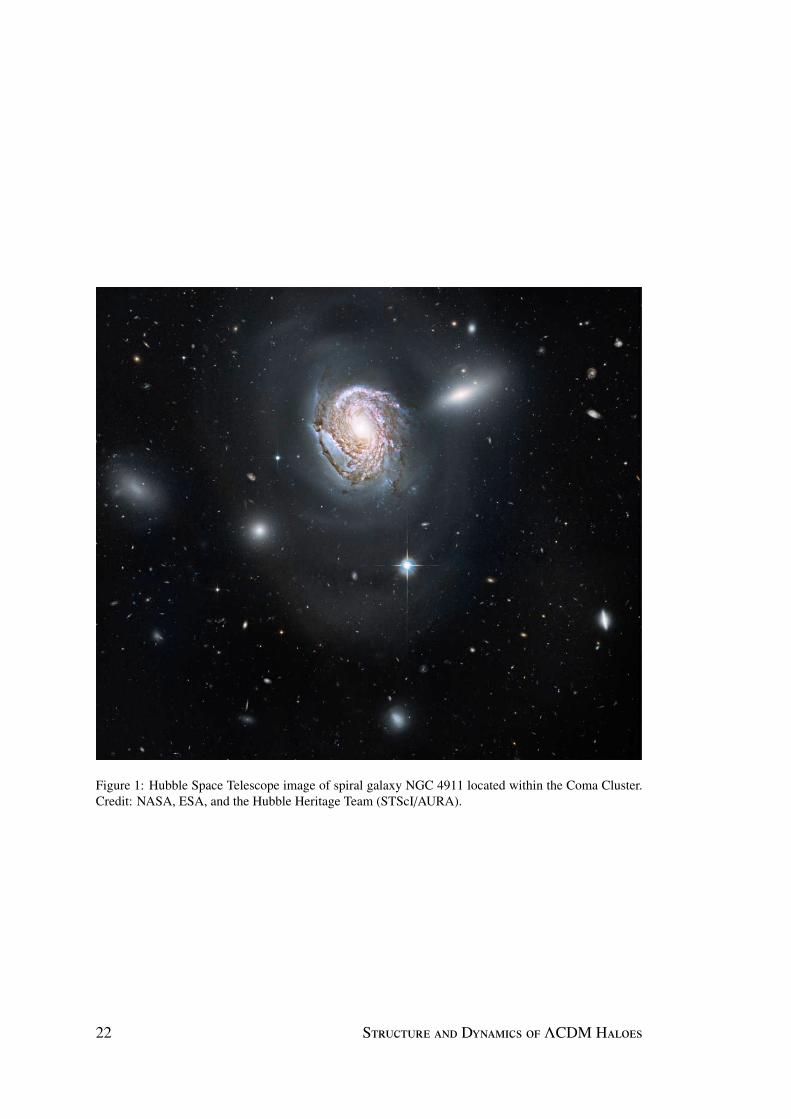
Figure 1: Hubble Space Telescope image of spiral galaxy NGC 4911 located within the Coma Cluster.Credit: NASA, ESA, and the Hubble Heritage Team (STScI/AURA).
22 S D ΛCDM H

1
Introduction
Attempts to understand our own Galaxy, its nature and origin, date back to Greek
philosophers such as Democritus and Aristotle in the 4th century BC. Understanding
our position in the cosmos, and how things came to be the way they are, are key ques-
tions that have naturally piqued the curiosity of mankind over millennia. Even today,
the complex nature of galaxy formation and evolution is not completely understood,
and is acknowledged as a key research area addressing some of the most fundamental
questions in astrophysics and cosmology.
While observations of the present day local Universe indicate an abundance of
structure (galaxies, clusters, filaments), measurements of the early Universe from the
Cosmic Microwave Background (CMB) paint a very different picture. The early Uni-
verse was initially very smooth. Exactly how the objects we see today formed and
evolved out of such smooth initial conditions is not an entirely solved problem and is
still an active area of research today. Fortunately, the last few decades have provided a
rapid increase in the amount of extragalactic data available, and this has contributed to-
wards a marked improvement in our understanding of the processes involved in galaxy
formation and evolution. The work presented in this thesis attempts to probe several
aspects of the formation process using state-of-the-art cosmological simulations.
As galaxies are thought to form and evolve within underlying dark matter struc-
tures, the morphology and kinematics of the dark matter will have important effects on
S E. B 23

1: INTRODUCTION
the development of the galaxies. Clearly a thorough understanding of these properties
is fundamentally important in furthering our knowledge of the formation and evolution
of galaxies.
Much progress has been made in revealing the nature of dark matter haloes thanks
to the rapid progression of computational techniques and advances in computational
resources. However, the role of baryons is much more uncertain. A detailed under-
standing of the role of baryons in galaxy formation and evolution is essential, not only
because most observations typically trace baryonic matter but also because of the com-
plex role it may play in the evolution of the dark matter halo itself.
The simulations used in this thesis provide a unique opportunity to analyse the
effects of baryons and implemented feedback techniques on a large sample of haloes
evolved within a cosmological setting.
The outline of this thesis is as follows. In chapter 2 the current cosmological model
is briefly reviewed and conventional views on the structure formation process in the
linear regime are introduced. The present status of comparisons of predictions from
this model with observations is also outlined. In chapter 3 the non-linear evolution
of structure is considered and a brief overview of commonly implemented simulation
techniques presented. Chapter 4 discusses lensing as a probe for substructure and com-
pares simulated predictions for the frequency of companion satellites to observations
of lens and field galaxies. Chapter 5 investigates the spin and shapes of dark matter
haloes in cosmological simulations and how these parameters are affected by bary-
onic physics. In chapter 6 the results of spectral analyses of the orbital content of these
haloes are presented and the effects of different implementations of feedback processes
are considered. A summary and discussion of the findings of this thesis can be found
in chapter 7.
24 S D ΛCDM H

2
The Standard Model of Cosmology
The standard cosmological model is intrinsically simple, based principally on General
Relativity (GR) and the assumptions of isotropy and homogeneity. The current model
has strong predictive power and has become well established both due to successful
comparison with a wide range of observations and due to the simplicity of the model.
According to this model, the Universe began ∼13 billion years ago in the Big Bang,
a point in time and space where the density and temperature of the Universe was ex-
treme. This idea extrapolates from the observation that the Universe is expanding
(Lemaıtre 1927; Hubble 1929) and was based on Hubble’s law: that all galaxies ap-
pear to be moving away from us and, the further away the galaxy, the faster it appears
to be receding. Recent observations based on high precision measurements of type Ia
supernovae (SNe Ia) at z ∼ 1 suggest that the expansion of the Universe is currently
accelerating (Perlmutter et al. 1999).
Within the standard model, the Universe consists of radiation, baryonic matter, cold
dark matter (CDM) and dark energy (Λ). The existence of dark matter was initially
proposed by Zwicky (1937), motivated by the difference in the dynamical virial mass
estimates and the observed luminous component of the Coma cluster. While dark
matter has not yet been detected directly there is a wealth of evidence now supporting
its existence (see section 2.1.1). Dark energy is an unknown force with a negative
pressure which is required to explain the current acceleration of the expansion of the
S E. B 25

2: THE STANDARD MODEL OF COSMOLOGY
Universe.
The hot dense initial conditions present in the Big Bang allow nucleosynthesis to
occur; this provides a prediction for the overall abundances of the elements (Chan-
drasekhar and Henrich 1942; Gamow 1946) and predicts the existence of a relic ther-
mal radiation field.
The discovery of the Cosmic Microwave Background (CMB) by Penzias and Wil-
son (1965) lead to general acceptance of the Big Bang model. The CMB radiation is
remarkably isotropic on angular scales from 1′ to 180. These regions were not ex-
pected to have been in causal contact, and as such there was no proposed mechanism
to explain how the temperatures were able to equalise. This is known as the Horizon
problem and is solved by inflation – a period of exponential expansion in the early
Universe (Guth 1981). All of the visible Universe would have been in causal contact
initially before experiencing exponential growth. Inflation provides solutions to sev-
eral other problems. It provides an origin of the initial density fluctuations (quantum
fluctuations). These density perturbations are assumed to grow via gravitational col-
lapse to form the structures we see today, with gas cooling radiatively to the centre of
the potentials formed by these structures. Inflation also provides an explanation for
the observed flatness of the Universe and predicts that the power spectrum should be
nearly scale invariant (these ideas are discussed in sections 2.1.1 and 2.2.2).
While the CMB initially appeared to have a uniform temperature, the tiny fluctua-
tions (of the order δT/T ∼ 10−5) that had been predicted by the standard model, were
detected by the COsmic Background Explorer (COBE, Smoot et al. 1992). More recent
observations of the CMB with the Wilkinson Microwave Anisotropy Probe (WMAP)
have led to an era of precision cosmology.
In this chapter a brief review of the current cosmological model and an introduction
to linear structure formation is presented. These sections describe the cosmological
framework used throughout this thesis. Some of the successes and challenges of this
paradigm are discussed. This chapter also describes how the initial conditions for the
simulations used in this work are generated and provides a definition for the structures
26 S D ΛCDM H

2.1: THE STANDARD PARADIGM
studied in later chapters.
Note that in this chapter natural units are assumed (in which the speed of light c
is set to 1); Greek indices run from 0 to 3; Latin indices from 1 to 3 and the Einstein
summation convention is assumed.
2.1 The Standard Paradigm
The fundamental framework of the standard model is based on the Cosmological Prin-
ciple, the Friedmann-Robertson-Walker (FRW) metric and the General Theory of Rel-
ativity (GR). The Cosmological Principle – that there are no preferred locations in the
Universe (see, for example, Weinberg 1972; Liddle 2003), implies that the properties
of the Universe are the same for all observers. Two consequences of this, that are
fundamentally important to this model, are the homogeneity and isotropy of the Uni-
verse. Current observations (such as: the isotropy of the CMB radiation; estimates
of the two-point correlation function and the power spectrum from the Sloan Digital
Sky Survey (SDSS) and the Two-degree Field (2dF) galaxy redshift survey; analysis
of deep radio surveys and multipoles of the X-ray background) support the assumption
that the Universe is homogeneous and isotropic on scales larger than ∼ 100 h−1 Mpc
(see Yadav et al. 2005 and references therein).
The FRW space-time metric provides a description of the geometry of a homoge-
neous, isotropic universe. This metric can be expressed as follows:
ds2 = gµνdxµdxν = dt2 − a2(t)
dr2
1 − kr2 + r2(dθ2 + sin2 θ dφ2
), (2.1)
where ds is the space-time element, a(t) is the scale factor (defined at the present
day as a0 ≡ a(t0) = 1) and (r, θ, φ) are the spatial coordinates at an arbitrary time t.
The trichotomic constant, k (determined by the energy density present), describes the
S E. B 27
2: THE STANDARD MODEL OF COSMOLOGY
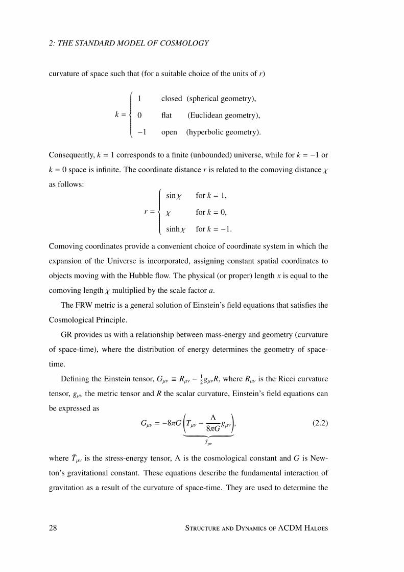
curvature of space such that (for a suitable choice of the units of r)
k =
1 closed (spherical geometry),
0 flat (Euclidean geometry),
−1 open (hyperbolic geometry).
Consequently, k = 1 corresponds to a finite (unbounded) universe, while for k = −1 or
k = 0 space is infinite. The coordinate distance r is related to the comoving distance χ
as follows:
r =
sin χ for k = 1,
χ for k = 0,
sinh χ for k = −1.
Comoving coordinates provide a convenient choice of coordinate system in which the
expansion of the Universe is incorporated, assigning constant spatial coordinates to
objects moving with the Hubble flow. The physical (or proper) length x is equal to the
comoving length χ multiplied by the scale factor a.
The FRW metric is a general solution of Einstein’s field equations that satisfies the
Cosmological Principle.
GR provides us with a relationship between mass-energy and geometry (curvature
of space-time), where the distribution of energy determines the geometry of space-
time.
Defining the Einstein tensor, Gµν ≡ Rµν − 12gµνR, where Rµν is the Ricci curvature
tensor, gµν the metric tensor and R the scalar curvature, Einstein’s field equations can
be expressed as
Gµν = −8πG(Tµν − Λ
8πGgµν
)
︸ ︷︷ ︸Tµν
, (2.2)
where Tµν is the stress-energy tensor, Λ is the cosmological constant and G is New-
ton’s gravitational constant. These equations describe the fundamental interaction of
gravitation as a result of the curvature of space-time. They are used to determine the
28 S D ΛCDM H

2.1: THE STANDARD PARADIGM
space-time geometry resulting from the presence of mass-energy and linear momen-
tum. Tµν is assumed to have the perfect fluid form
Tµν = pgµν + (ρ + p) UµUν, (2.3)
where ρ denotes the total energy density, p is the total pressure density and Uµ is a
velocity four-vector in which U0 = 1 and Ui = 0.
From the energy conservation equation ∇µTµν = 0, one has
˙ρ + 3H (ρ + p) = 0. (2.4)
Here the Hubble parameter H describes the rate of expansion of the Universe and is
defined as H ≡ a/a. The Hubble parameter measured at the present day is known as
the Hubble constant, and is often expressed as H0 = 100 h km s−1Mpc−1, where h is
a dimensionless constant (this convention is adopted for this thesis). Substituting the
FRW metric and the perfect fluid energy momentum tensor Tµν (2.3) into Einstein’s
equations (2.2) gives
H + H2 = −4πG3
(ρ + 3p)(00 − component
), (2.5a)
H + 3H2 = 4πG (ρ − p)(ii − component
). (2.5b)
The density and pressure content of the Universe are expressed as ρ and p, respectively.
The total density content ρ is given by the sum of the components ρ = ρ + ρΛ + ρk =
ρr +ρm +ρΛ +ρk, where ρr and ρm refer to the energy density of radiation and matter re-
spectively and contributions from the curvature, k, and cosmological constant, Λ, have
also been written in terms of energy density as ρΛ = Λ/8πG and ρk = −3k/8πGa2.
The pressure term p is the total pressure density p = p + pΛ + pk = pr + pm + pΛ + pk.
Substituting (2.5a) into (2.5b) gives the Friedmann equation
H2 =
( aa
)2
=8πG
3ρ. (2.6)
S E. B 29

2: THE STANDARD MODEL OF COSMOLOGY
The Friedmann equation (2.6) and the energy conservation equation (2.4) govern the
dynamics of the Universe which are driven by the energy content ρ. In addition, one
must specify the equation of state, which relates pressure to density as
pi = ωiρi, (2.7)
where i refers to the components r,m, k,Λ. Components are separated according to
their equation of state into: radiation and relativistic matter (ωr = 1/3); non-relativistic
matter (ωm = 0); the contribution of curvature (ωk = −1/3) and a positive vacuum en-
ergy density (assumed to be constant for simplicity) associated with the cosmological
constant term in Einstein’s Field Equations (ωΛ = −1). The pressure density from each
component is then given by: pr = 13ρr; pm = 0; pΛ = −ρΛ = − Λ
8πG ; pk = −13ρk = k
8πGa2 .
The three equations (2.4), (2.6) and (2.7) are the fundamental equations describing
the dynamics of an expanding, isotropic and homogeneous universe. The total energy
content plays a critical role in deciding the fate of the Universe.
At the present day, the Friedmann equation (2.6) can be rearranged as
ρ0 =3
8πG
(H2
0 + k), (2.8)
where the curvature component has been separated from the rest of the mass/energy
terms. Defining a critical density
ρcrit =3H2
8πG, (2.9)
the current energy density (2.8) can be expressed as
ρ0 = ρcrit,0 +3k
8πG. (2.10)
In (2.10), k = 0 corresponds to ρ0 = ρcrit and a flat universe. An open universe (k < 0
and ρ0 < ρcrit) expands forever, while in a closed universe (k > 0 and ρ0 > ρcrit)
30 S D ΛCDM H

2.1: THE STANDARD PARADIGM
expansion ceases and a general contraction will occur.
Dividing (2.10) by ρcrit,0, results in normalised energy densities
Ωtotal = Ωr + Ωm + ΩΛ = 1 +k
H20
. (2.11)
In this way the condition for closure can be expressed as Ωtotal > 1; a flat universe has
Ωtotal = 1 and an open universe has Ωtotal < 1. The value of ρcrit is estimated to be
2.78 × 10¹¹ h2 M Mpc −3 or 1.88 × 10⁻²⁹ h2 g cm−3 (Kolb and Turner 1993).
In order to discuss the scaling behaviour of the energy components with the scale
factor, the energy conservation equation (2.4) is re-expressed as
dda
(ρa3
)= −3pa2. (2.12)
Substituting the equation of state (2.7) into (2.12) and integrating gives
ρ ∝ a−3(1+ω). (2.13)
Substituting the scaling behaviour of ρ in (2.13) into the Friedmann equation (2.6) and
integrating gives the time evolution of the scale factor
a ∝ t2/3(1+w). (2.14)
It is then trivial to show the time dependence of the scale factor for each of the epochs:
a ∝ t1/2 in the radiation-dominated era and a ∝ t2/3 in the matter-dominated era. For
the cosmological constant, ρΛ is constant, and the Friedmann equation simplifies to
H = a/a = constant. Integrating this equation shows that in this era the scale factor
grows exponentially as a ∝ eHt.
Rewriting (2.5a) as
aa
= −4πG3
(ρ + 3p) = −4πG3
(ρ + 3p) +Λ
3, (2.15)
S E. B 31

2: THE STANDARD MODEL OF COSMOLOGY
and assuming ρ > 0, p > 0 and Λ = 0 gives a/a < 0. Since the observed a > 0
(redshifts are observed) a(t) is concave. This implies that at some finite point in time
the scale factor was zero and, ipso facto, a Big Bang. The time to when a = 0 defines
a maximum bound for the age of the Universe t0. For a = 0, a is constant. One can
therefore write a = (a0/t0) t = (da/dt) t. Consequently t0 = (a0/a) t and t0 = a0/a0 =
1/H0. Early (inaccurate) measurements of the Hubble constant resulted in the age
paradox (see, for example, the discussion in Earman 2001) – where predicted values
of t0 were much shorter than the age of the earth (as determined by radioactive decay)
and the ages of the stars (as determined by stellar evolution theory).
2.1.1 Current Parameters in the Standard Model
The previous section describes the theoretical framework of modern cosmology, ΛCDM.
This model is fully described by only six parameters, namely: the matter density Ωmh2;
the baryon density Ωbh2; the Hubble constant H0; the root mean squared amplitude of
fluctuations σ8 (defined within a sphere of 8h−1Mpc at z = 0); the integrated optical
depth τ (=∫ zr
0σT ne (z) dt
dzdz where zr is the redshift of reionisation, σT is the Thomson
scattering cross-section and ne the number density of free electrons) and the slope of
the scalar perturbation spectrum ns. The amplitude of this spectrum is given by ∆2R and
is conventionally defined at the pivot scale k0 = 0.002 Mpc−1.
Constraints on these cosmological parameters are most commonly derived from
observations of the CMB; additional orthogonal constraints are provided by SNe Ia
and Baryonic Acoustic Oscillations (BAO). The joint constraints on the Ωm−ΩΛ plane
are shown in figure 2.1. These observations are discussed briefly below.
Supernovae Ia. SNe Ia are calibratable distance indicators (Riess et al. 1996). Since
distance depends on the underlying cosmology, using the observed redshift with luminosity-
distance relation places constraints on the cosmological parameters h,Ωm and ΩΛ. Ob-
servations based on high-precision measurements of SNe Ia (Riess et al. 1998; Gar-
navich et al. 1998; Perlmutter et al. 1999; Kowalski et al. 2008) at high redshift find
32 S D ΛCDM H

2.1: THE STANDARD PARADIGM
Figure 2.1: Joint constraints on the Ωm−ΩΛ plane from SNe data, BAO and CMB observations (assum-ing ω = −1), contours show the 1,2 and 3 σ confidence levels. Taken from Kowalski et al. (2008).
that these SNe are fainter than expected, implying an accelerating expansion of the
Universe at late times. Two possible explanations have been put forward: either GR
breaks down at large scales and a modified theory of gravity is required (for example
MOdified Newtonian Dynamics or MOND), or there is an unknown energy content
with a negative pressure which is driving the expansion. The unknown energy content
has been termed dark energy and is described by an equation of state ω ≤ −1/3. The
standard model assumes a cosmological constant Λ with ω = −1; however ω may vary
with time.
Cosmic Microwave Background. The CMB provides a measure of the surface of
last scattering. The detailed pattern of anisotropies observed in the CMB power spec-
S E. B 33
2: THE STANDARD MODEL OF COSMOLOGY
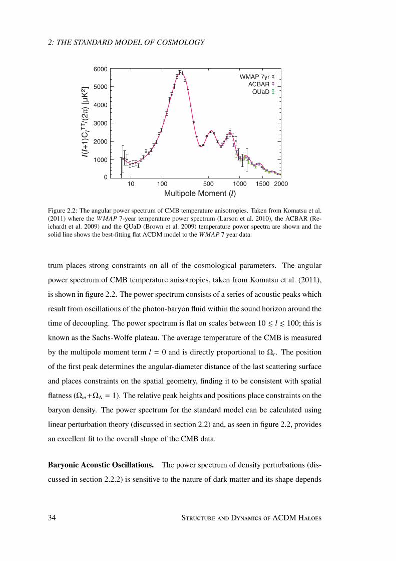
Figure 2.2: The angular power spectrum of CMB temperature anisotropies. Taken from Komatsu et al.(2011) where the WMAP 7-year temperature power spectrum (Larson et al. 2010), the ACBAR (Re-ichardt et al. 2009) and the QUaD (Brown et al. 2009) temperature power spectra are shown and thesolid line shows the best-fitting flat ΛCDM model to the WMAP 7 year data.
trum places strong constraints on all of the cosmological parameters. The angular
power spectrum of CMB temperature anisotropies, taken from Komatsu et al. (2011),
is shown in figure 2.2. The power spectrum consists of a series of acoustic peaks which
result from oscillations of the photon-baryon fluid within the sound horizon around the
time of decoupling. The power spectrum is flat on scales between 10 . l . 100; this is
known as the Sachs-Wolfe plateau. The average temperature of the CMB is measured
by the multipole moment term l = 0 and is directly proportional to Ωr. The position
of the first peak determines the angular-diameter distance of the last scattering surface
and places constraints on the spatial geometry, finding it to be consistent with spatial
flatness (Ωm +ΩΛ = 1). The relative peak heights and positions place constraints on the
baryon density. The power spectrum for the standard model can be calculated using
linear perturbation theory (discussed in section 2.2) and, as seen in figure 2.2, provides
an excellent fit to the overall shape of the CMB data.
Baryonic Acoustic Oscillations. The power spectrum of density perturbations (dis-
cussed in section 2.2.2) is sensitive to the nature of dark matter and its shape depends
34 S D ΛCDM H

2.1: THE STANDARD PARADIGM
Table 2.1: Current values of the cosmological parameters from Komatsu et al. (2011).WMAP7 WMAP7 + SNe + BAO
100Ωb h2 2.249+0.056−0.057 2.255 ± 0.054
ΩCDM h2 0.1120 ± 0.0056 0.1126 ± 0.0036ΩΛ h2 0.727+0.030
−0.029 0.725 ± 0.016ns 0.967 ± 0.014 0.968 ± 0.012τ 0.088 ± 0.015 0.088 ± 0.014
∆2R × 109 2.43 ± 0.11 2.430 ± 0.091
h 0.704 ± 0.025 0.702 ± 0.014σ8 0.811+0.030
−0.031 0.816 ± 0.024Ωb 0.0455 ± 0.0028 0.0458 ± 0.0016
ΩCDM 0.228 ± 0.0027 0.229 ± 0.015Ωm h2 0.1345+0.0056
−0.0055 0.1352 ± 0.0036t0 13.77 ± 0.13 Gyr 13.76 ± 0.11 Gyr
on the primordial power spectrum and the horizon scale at matter-radiation equality
(determined by Ωmh). The simplest way to probe the matter distribution is to observe
the distribution of galaxies. However galaxies are a biased tracer of the underlying
matter distribution; they cluster in regions of high density and different galaxy types
show a bias with respect to each other. On large scales the galaxy power spectrum is
thought to be a constant multiple b of the dark matter spectrum. On smaller scales co-
herent infall acts to compress the clustering in the radial direction. The galaxy power
spectrum has been measured by 2dF and SDSS and is well-fit by the ΛCDM model.
Both of these surveys show evidence for BAOs which can be used as standard rulers.
Joint Constraints. Quite remarkably all of these measurements (SNe Ia, BAO and
measurements of the CMB) intersect on the Ωm −ΩΛ plane, placing strong constraints
on the cosmological parameters, indicating that the Universe is flat and experiencing
an epoch of accelerating expansion. The current values for these parameters as derived
from these joint constraints (WMAP7, SNe Ia and BAOs) are given in Komatsu et al.
(2011) and are summarised in table 2.1.
In summary, within the standard model the present day Universe is made up of
radiation (negligible contribution), baryonic matter (4%), cold dark matter (CDM ∼26%) and dark energy (Λ ∼ 70%). The Universe is modelled as isotropic, homogenous
S E. B 35

2: THE STANDARD MODEL OF COSMOLOGY
and flat (Ωm + ΩΛ = 1). The model also assumes a nearly scale invariant spectrum of
primordial fluctuations (ns ∼ 1). Flatness and scale-invariance are both explained by
cosmic inflation, a period of exponential expansion in the very early Universe. Dark
energy, also known as the cosmological constant, makes up most of the total mass-
energy of the present day Universe. This energy has a strong negative pressure and is
thought to be responsible for the accelerating expansion of the Universe at late times.
Most of the remaining mass of the Universe is made up of cold dark matter, which is
non-baryonic and collisionless.
Dark Matter Candidates
Dark matter interacts primarily through gravity (although weak interactions cannot be
ruled out), making direct detection an arduous task. Dark matter is collisionless and
assumed to be cold, that is, non-relativistic at the time of decoupling. Hot dark matter
models are ruled out through observations of small scale structure, the non-negligible
velocities of hot dark matter particles has a dramatic effect on these scales (see section
2.2.2).
Cold dark matter provides an excellent fit to many observations, but some doubt
remains on small scales such as the structure of dwarf galaxies and substructure in
galaxy haloes. Dark matter plays an important role in structure formation, providing
potential wells that enhance the collapse rate of baryons, allowing structure to form on
observed time-frames. Further evidence for dark matter is provided by objects such as
the Bullet cluster (Clowe et al. 2006) – a merging cluster of galaxies in which the centre
of mass determined from the hot gas (observed in X-rays) is displaced from the centre
of mass as determined from lensing. A natural explanation arises if collisionless dark
matter dominates the potential, while the hot gas interacts during the merging process.
Candidates for dark matter include axions, primordial black holes and weakly in-
teracting massive particles (WIMPs). Dark matter has not yet been directly detected.
Direct searches for WIMPs (e.g. light supersymmetric particles) attempt to observe
signatures from nuclear recoil. Complementary to the direct detection methods are
36 S D ΛCDM H

2.2: AN INTRODUCTION TO LINEAR STRUCTURE FORMATION
indirect methods such as the search for gamma-ray self-annihilation signals.
2.2 An Introduction to Linear Structure Formation
Small fluctuations in the temperature of the CMB imply that there are inhomogeneities
in the early Universe, the size of which constrain the amplitude of the density pertur-
bations at this time. In order to understand how these tiny fluctuations transform into
the structure seen today, a brief introduction to structure formation in the linear regime
is given in this section. The details of numerical simulation of structure formation in
the non-linear regime can be found in chapter 3.
The standard model assumes that random quantum fluctuations present in the very
early Universe grow via gravitational instabilities into the structure observed today.
Structure formation began at the time of matter-radiation equality, teq, when matter
began to dominate the Universe and baryons are freed from the pressure support of
photons.
To study structure formation in the linear regime small, linear, adiabatic perturba-
tions in the FRW metric (2.1) are considered and the growth of these perturbations
in a homogeneous background with a mean background density ρ (t) = 3H2/8πG is
followed. The density perturbations are described as ρ = ρ (t) (1 + δ (x, t)), in terms of
their density contrast or amplitude δ (where, in the linear regime, δ 1). The density
contrast δ (x) can be expressed in terms of the overdensity relative to the background
density as
δ (x) ≡ δρ (x)ρ
=ρ (x) − ρ
ρ. (2.16)
The density contrast δ (x) can be related to a curvature term (as in Kolb and Turner
1993). Relating the mean background density ρ to the density of a flat FRW model
gives
H2 =8πG
3ρ⇒ ρ =
38πG
H2. (2.17)
S E. B 37

2: THE STANDARD MODEL OF COSMOLOGY
Considering a perturbation to this model (without changing the Hubble constant H)
where the density ρ > ρ implies k > 0 and gives
H2 =8πG
3ρ − k
a2 ⇒ ρ =3
8πG
(H2 +
ka2
). (2.18)
The density contrast can then be written as
δ =ρ − ρρ
=k
a2H2 =k/a2
8πGρ/3∝ k/a2
ρ∝ ka1+3ω. (2.19)
Where the scaling relation (2.14) has been used in the last step. Consequently, an over-
density can be thought of as a closed universe which will collapse, becoming increas-
ingly overdense. Whereas an underdensity, like an open universe, will keep expanding
and become increasingly underdense.
The density contrast can also be written in terms of a Fourier expansion (valid in
spatially flat models) as
δk =1V
∫
Vδ (x) exp (−ik · x) d3x, (2.20)
where periodic boundary conditions have been imposed and V is the volume of the
fundamental cube. The Fourier components are completely characterised by their
amplitudes |δk|, and the comoving wavenumber k. The comoving wavelength of a
perturbation is related to the wavenumber as λ ≡ 2π/k, where the physical wave-
length λphys = a (t) λ describes the physical length scale of perturbations. In curved
space-time, the plane wave solutions are replaced by the generalised solution to the
Helmholtz equation.
Structures form via the collapse of perturbations under gravity. This can only occur
in regions that are in causal contact. This region is described by the horizon scale, rH.
If one considers light emitted at the horizon (rH) at t = 0 and observed at r = 0 at
time t, then a photon travelling along a null radial geodesic (where ds2 = 0 and dθ =
38 S D ΛCDM H
2.2: AN INTRODUCTION TO LINEAR STRUCTURE FORMATION
dφ = 0) in the FRW metric (2.1) gives
dt2 = a (t)2 dr2
1 − kr2 . (2.21)
This can be rewritten as ∫ t
0
dta (t)
=
∫ rH
0
dr√1 − kr2
, (2.22)
and the comoving horizon rH in a flat universe (with k = 0) can be expressed as
rH =
∫ t
0
dta (t)
=
∫dtda
daa (t)
=
∫da
a2H=
∫da
a2√(
a−3(1+ω)) ∝ a1/2(1+3w). (2.23)
In the radiation-dominated era the comoving horizon grows as rH ∝ a, while in the
matter-dominated era it grows as rH ∝ a1/2. When the energy density is dominated
by the cosmological constant the comoving horizon scales as rH ∝ a−1. The proper
horizon is given by dH = a (t) rH. From this it can be seen that fluctuations which
are expanded out of the horizon during inflation can re-enter the horizon during the
radiation- and matter-dominated eras. The smallest-scale fluctuations will re-enter and
collapse before larger-scale fluctuations. During the Λ-dominated era the comoving
horizon size decreases and ever smaller scales remain causally connected. Using ρ ∝a−3(1+w) and H2 ∝ ρ, one can easily show that dH ∝ H−1. It is worth noting that the
proper horizon does not grow in the Λ-dominated era.
There are two characteristic regimes divided, depending on the size of the pertur-
bations, into either super- or sub-horizon scales. In the early regime, density pertur-
bations are super-horizon-sized. Here the gauge invariance of δρ/ρ needs to be con-
sidered and the distinction between isocurvature and adiabatic density perturbations
is important. Adiabatic perturbations correspond to fluctuations in the spatial curva-
ture, while isocurvature perturbations correspond to spatial variations in the equation
of state. Isocurvature perturbations correspond to perturbations of the relative amounts
of the different components while the total energy density remains constant. In the
early regime a full general relativistic treatment is required. In the later regime, where
S E. B 39
2: THE STANDARD MODEL OF COSMOLOGY
modes are well within the horizon and gravitational collapse is possible, Newtonian
analysis is sufficient (Newtonian analysis becomes exact as λphys/H−1 → 0).
2.2.1 Linear Perturbation Growth in the Newtonian Regime
The first recognised theory of galaxy formation was proposed by Jeans (1928) who
described the Universe as a non-relativistic perfect fluid with mass density ρ, pressure
p and velocity v under the influence of a gravitational field with potential φ. In Jeans’
analysis small perturbations to a static uniform fluid were considered. Unfortunately,
the assumption of a static medium implies that perturbation growth in an expanding
universe cannot be explored. The case for an expanding universe was first consid-
ered by Bonnor (1957). In the case of an expanding fluid, structure formation in the
Newtonian limit, is governed by the following equations:
∂δ
∂t+ ∇ · [(1 + δ) v] = 0, (2.24)
∂v∂t
+aa
v + (v · ∇) v +∇pρ
+ ∇φ = 0, (2.25)
∇2φ = 4πGρδ. (2.26)
These equations are the perturbed versions of the continuity equation, the Euler equa-
tion and Poisson’s equation respectively. Combining the first-order perturbed fluid
equations (2.24 - 2.26), one derives the following second-order differential equation
for the density fluctuations:
δm + 2aaδm + δm
(c2
sk2
a2 − 4πGρm
)= 0, (2.27)
where the speed of sound is defined as
c2s ≡
(∂p∂ρ
), (2.28)
where the differentiation is taken with respect to adiabatic changes.
40 S D ΛCDM H

2.2: AN INTRODUCTION TO LINEAR STRUCTURE FORMATION
Solutions to the growth equation (2.27) can be considered within the different
epochs of the Universe defined by the dominant energy content.
During the radiation-dominated era fluctuations do not grow as perturbation growth
is suppressed by radiation pressure, and the perturbations oscillate as acoustic waves
with a constant amplitude. The photon pressure of baryonic fluctuations entering the
horizon sets the Jeans length scale LJ (critical scale above which gravitational collapse
will occur) to be of the order of the horizon scale. The Jeans stability argument sets
the sound crossing time tsc to be less than the dynamical time tdyn or
LJ
cs<
1√Gρ∼ 1
H∼ t. (2.29)
Before decoupling the speed of sound cs in the relativistic plasma is ∼ c√3
and the
Jeans length is of the order of the horizon scale (LJ ∼ c t ∼ rH). Perturbations are
unable to collapse. During the radiation era CDM fluctuations are suppressed by the
Meszaros Effect (Meszaros 1974): expansion of the universe is so fast that the dark
matter does not have enough time to respond and collapse and the density fluctuations
δ are effectively frozen out. Comparing the expansion time-scale texp = 1/H to the
dynamical timescale tdyn expressed in terms of the dark matter density ρdm,
1H∼ 1√
Gρr<
1√Gρdm
, (2.30)
shows that expansion rate in this era prevents the collapse of dark matter perturbations.
In the matter-dominated regime, dark matter fluctuations grow as δ ∝ a, while the
growth of baryonic fluctuations is delayed as baryons and photons are coupled until
recombination, at which point the baryons are free from radiation pressure and fall
into the enhanced potentials that have already been created by the dark matter. Once Λ
begins to dominate, the comoving horizon scale shrinks and ever smaller regions are
within causal contact, eventually freezing out structure formation.
S E. B 41
2: THE STANDARD MODEL OF COSMOLOGY
2.2.2 The Power Spectrum
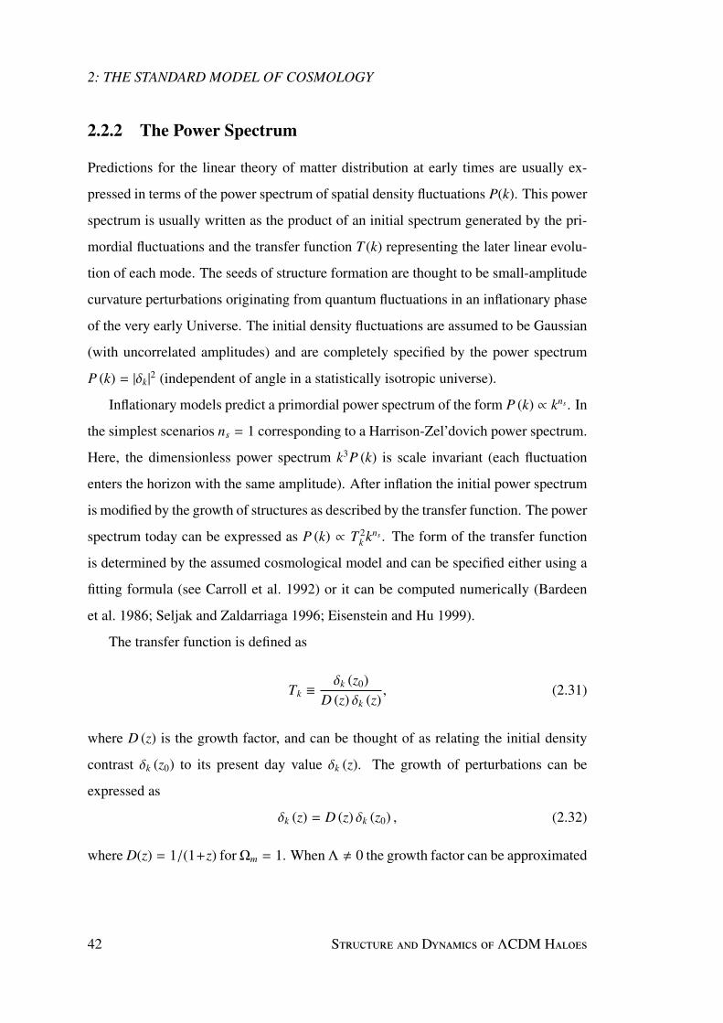
Predictions for the linear theory of matter distribution at early times are usually ex-
pressed in terms of the power spectrum of spatial density fluctuations P(k). This power
spectrum is usually written as the product of an initial spectrum generated by the pri-
mordial fluctuations and the transfer function T (k) representing the later linear evolu-
tion of each mode. The seeds of structure formation are thought to be small-amplitude
curvature perturbations originating from quantum fluctuations in an inflationary phase
of the very early Universe. The initial density fluctuations are assumed to be Gaussian
(with uncorrelated amplitudes) and are completely specified by the power spectrum
P (k) = |δk|2 (independent of angle in a statistically isotropic universe).
Inflationary models predict a primordial power spectrum of the form P (k) ∝ kns . In
the simplest scenarios ns = 1 corresponding to a Harrison-Zel’dovich power spectrum.
Here, the dimensionless power spectrum k3P (k) is scale invariant (each fluctuation
enters the horizon with the same amplitude). After inflation the initial power spectrum
is modified by the growth of structures as described by the transfer function. The power
spectrum today can be expressed as P (k) ∝ T 2k kns . The form of the transfer function
is determined by the assumed cosmological model and can be specified either using a
fitting formula (see Carroll et al. 1992) or it can be computed numerically (Bardeen
et al. 1986; Seljak and Zaldarriaga 1996; Eisenstein and Hu 1999).
The transfer function is defined as
Tk ≡ δk (z0)D (z) δk (z)
, (2.31)
where D (z) is the growth factor, and can be thought of as relating the initial density
contrast δk (z0) to its present day value δk (z). The growth of perturbations can be
expressed as
δk (z) = D (z) δk (z0) , (2.32)
where D(z) = 1/(1+z) for Ωm = 1. When Λ , 0 the growth factor can be approximated
42 S D ΛCDM H

2.2: AN INTRODUCTION TO LINEAR STRUCTURE FORMATION
Figure 2.3: The transfer functions of various models taken from Nakamura and Group (2010).
using a fitting formula (for more details see, for example, Peebles 1980; Carroll et al.
1992 or Eisenstein and Hu 1999).
The transfer functions for various models are shown in figure 2.3. Note that after
recombination the baryonic Jeans scale drops suddenly to small scales due to the rapid
decrease in pressure. CDM fluctuations are also suppressed before equality (keq ∼ 20 h
kpc−1) by the Meszaros Effect (see previous discussion). There are also dissipational
effects (such as Silk damping in the case of baryons or Landau damping in the case
of hot dark matter) that must be considered when the perfect fluid assumption breaks
down.
As the Universe cools and recombination is approached, the mean free path of pho-
tons increases, photons diffuse out of high density regions into lower density regions
smoothing out inhomogeneities. This photon diffusion is known as Silk damping. The
Silk damping scale sets a smoothing length for the perturbations, beyond which struc-
S E. B 43
2: THE STANDARD MODEL OF COSMOLOGY
ture is not expected to form.
Nearly collisionless components such as neutrinos or hot/warm dark matter parti-
cles undergo free streaming or Landau damping. The growth of structures on scales
smaller than the free streaming length λFS is strongly suppressed until equality when
perturbations become Jeans unstable and begin to grow effectively suppressing the
growth of small scale haloes. Following freeze-out of dark matter interactions, dark
matter particles will free stream over a distance determined by their thermal velocity.
Density fluctuations smaller than this free streaming length are highly suppressed. The
smallest haloes which arise are expected to have masses of the order
MFS =4π3ρmλ
3FS . (2.33)
Smaller haloes could potentially form through non-hierarchical processes such as frag-
mentation. In warm dark matter models the temperature of dark matter particles is cho-
sen to make free-streaming length correspond to subgalactic scales λFS ∼ 0.1 h−1 Mpc
(see, for example, the discussion in Bode et al. 2001).
Small k modes enter the horizon and are causally connected later than large k
modes; they are therefore less susceptible to damping.
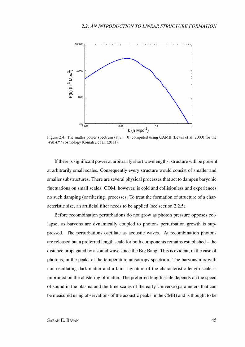
The scaling of the present day power spectrum P (k) = AT 2k kns can be inferred by
considering the evolution of the perturbations as a function of the era in which the
perturbation crosses the horizon:
P (k) ∝
kns−4 k keq,
kns k keq.
The power spectrum is normalised by σ8 the root mean square deviation of density
fluctuations within an 8 h−1 Mpc sphere at z = 0. The spectral index ns and normalisa-
tion σ8 are key cosmological parameters which fully determine the fluctuation power
spectrum. The matter power spectrum (at z = 0) for WMAP7 cosmological parameters
is shown in figure 2.4.
44 S D ΛCDM H
2.2: AN INTRODUCTION TO LINEAR STRUCTURE FORMATION
100
1000
10000
100000
0.001 0.01 0.1 1
P(k
) (h
-3 M
pc3 )
k (h Mpc-1)
Figure 2.4: The matter power spectrum (at z = 0) computed using CAMB (Lewis et al. 2000) for theWMAP7 cosmology Komatsu et al. (2011).
If there is significant power at arbitrarily short wavelengths, structure will be present
at arbitrarily small scales. Consequently every structure would consist of smaller and
smaller substructures. There are several physical processes that act to dampen baryonic
fluctuations on small scales. CDM, however, is cold and collisionless and experiences
no such damping (or filtering) processes. To treat the formation of structure of a char-
acteristic size, an artificial filter needs to be applied (see section 2.2.5).
Before recombination perturbations do not grow as photon pressure opposes col-
lapse; as baryons are dynamically coupled to photons perturbation growth is sup-
pressed. The perturbations oscillate as acoustic waves. At recombination photons
are released but a preferred length scale for both components remains established – the
distance propagated by a sound wave since the Big Bang. This is evident, in the case of
photons, in the peaks of the temperature anisotropy spectrum. The baryons mix with
non-oscillating dark matter and a faint signature of the characteristic length scale is
imprinted on the clustering of matter. The preferred length scale depends on the speed
of sound in the plasma and the time scales of the early Universe (parameters that can
be measured using observations of the acoustic peaks in the CMB) and is thought to be
S E. B 45

2: THE STANDARD MODEL OF COSMOLOGY
∼ 140 Mpc (Eisenstein 2005). This length scale is apparent as a peak in the two-point
correlation function and can be seen as a series of faint wiggles in the power spectrum
(BAOs).
2.2.3 Zel’dovich Approximation
An efficient method for setting up initial conditions from a given power spectrum is
provided by the Zel’dovich (1970) formulation of linear evolution of a general distribu-
tion of fluctuations. This formalism provides a first order approximation to Lagrangian
perturbation theory (LPT). Formalisms involving second order approximations (2LPT)
are also considered for large scale simulations (as in Jenkins 2010). The simulations
considered in this work are small enough that the first order approximation will suf-
fice; for this reason only the Zel’dovich approximation is discussed here (following the
approach given in White 1996).
The density contrast expressed in terms of the growth factor equation (2.32) implies
that density grows self-similarly with time. Substituting equation (2.32) into Poisson’s
equation (2.26) shows that this is also true for the gravitational acceleration ∇φ. The
gravitational potential φ scales with the expansion factor a as
φ (x, z) =D(z)
aφ0 (x) , (2.34)
where φ0 fulfils the perturbed Poisson equation (2.26)
∇2φ0 (x) = 4πGρa3δ0 (x) . (2.35)
In an Einstein-de Sitter universe (where Λ = P = 0) D ∝ a, implying that φ is inde-
pendent of the conformal time η (where adη = dt). The linearised version of Euler’s
equation (2.25) can be integrated with respect to η as follows:
v = −(a−1
∫Ddη
)∇φ0 = −
(D−1
∫Ddη
)∇φ. (2.36)
46 S D ΛCDM H

2.2: AN INTRODUCTION TO LINEAR STRUCTURE FORMATION
Note that the peculiar velocity v is proportional to the current gravitational acceleration
∇φ. A second integration yields
x = x0 −(∫
dηa
∫Ddη
)∇φ0. (2.37)
Since D (η) satisfies the linearised version of the perturbation growth equation (2.27)
aδ + aδ = 4πGρa3δ the double integral is proportional to D and the above equations
can be written as
x = x0 − D (η)4πGρa3∇φ0, (2.38)
v = − D (η)4πGρa2∇φ0 = − 1
4πGρa2
aDD∇φ, (2.39)
where the scaling relation (2.34) has been used in the last step.
Given a displacement x − x0 and the peculiar velocity v of every particle, this
formalism describes the growth of structure as a function of its initial position x0.
Zel’dovich (1970) proposed that these equations could be extrapolated to describe the
evolution of structure when displacements are no longer small. Given the growth of
structure (as described by the power spectrum), this approximation can be used to
establish the initial positions and velocities of a particle distribution and is used to set
up the initial conditions for the simulations used in this thesis.
2.2.4 Non-Linear Collapse and the Definition of Haloes
When perturbations grow to the point δρ/ρ & 1 linear perturbation theory breaks down.
While a full treatment of the non-linear regime can only be computed numerically (dis-
cussed in the next chapter), simple approximations to this complicated era are consid-
ered here in order to define what is meant by a halo.
The simplest approximation for non-linear growth is given by the spherical top-
hat collapse model (discussed in many texts including Kolb and Turner 1993). The
spherical top-hat model considers a spherical region with uniform overdensity δ and
S E. B 47
2: THE STANDARD MODEL OF COSMOLOGY
radius r in an otherwise uniform background described by a flat homogeneous matter
dominated FRW model.
The spherical region will decouple from the expansion at ‘turn-around’ and will
begin to collapse. Taylor expanding the parametric solutions of the energy equation
E =12
r − 43πGρr2, (2.40)
shows that the overdensity δρ/ρ = 9π2/16 at ‘turn-around’. After reaching this maxi-
mum size, the region will collapse and virialise. Such virialised structures are known
as haloes. After virialisation the kinetic energy is equal to half the gravitational po-
tential energy. Equating the total energy before and after virialisation (assuming no
dissipative forces) one finds that rvir = rmax/2. Since ‘turn-around’ the region has
halved its size, correspondingly its density has increased by a factor of 8. In the time
since ‘turn-around’ the universe has expanded by 22/3 and is therefore less dense by a
factor of 4. Hence, in an Einstein-de Sitter model virialised haloes have overdensities
of ∆c = ρ/ρcrit = 18π2 ≈ 200.
Spherical collapse within open, low mass-density universes with ΩΛ = 0 is consid-
ered in Lacey and Cole (1993a) and in a flat ΛCDM universe with Ωr = 0 in Eke et al.
(1996). Bryan and Norman (1998) provide a simple quadratic fit for the overdensity,
normalising from simulations. They find
∆c = 18π2 + 82x − 39x2, (2.41)
where x = Ω (z) − 1, Ω (z) = Ωm (1 + z)3 /E (z)2 and
E2 = Ωm (1 + z)3 + Ωr (1 + z)2 + ΩΛ. (2.42)
In the standard cosmology ∆c ∼ 92.5 at z = 0 and ∆c ∼ 168 at z = 2.
Haloes and their boundaries can be defined by an overdensity ∆ and the radius r∆ at
which the overdensity is reached. The mass contained within the radius of this sphere
48 S D ΛCDM H

2.2: AN INTRODUCTION TO LINEAR STRUCTURE FORMATION
is M∆ = 43 π r3
∆∆ ρcrit (z), where the mean internal density is ∆ times the critical density
at that redshift. The virial radius r∆ = rvir and associated virial mass, M∆ = Mvir are
defined by setting ∆ = ∆c from the spherical top-hat collapse model. Extensions to this
model such as the ellipsoid top-hat model will not be considered here.
2.2.5 Statistics of Hierarchical Clustering
In order to follow the evolution of dark matter haloes one requires an understanding
of hierarchical clustering. As discussed in White (1996), this allows one to address
fundamental issues such as the the origin of the mass function of galaxies and galaxy
clusters, the differences between galaxies and clusters despite the fact they both form
via gravitational collapse, rates of mergers and the relationship between a galaxy and
its large-scale environment. There are two general approaches which have been used
to this effect: the peak-formalism and Press-Schechter theory (Press and Schechter
1974). Both of these approaches assume Gaussian random field initial conditions.
The peak formalism assumes that the matter that will eventually collapse to form
a halo can be identified by locating peaks in the initial density field after smoothing
with a filter of an appropriate scale. Haloes are defined as regions where high density
peaks have risen above a fixed collapse threshold. This naturally introduces a bias in
that haloes will be tend to cluster in high density regions. This approach is detailed in
Bardeen et al. (1986) where statistical peak properties (such as height and shape) are
used to calculate the abundance and clustering properties of objects.
The second approach is based on the theory developed by Press and Schechter
(1974) and extended by Sheth and Tormen (2004). In this approach, the density field is
smoothed by a top-hat filter function; density perturbations that grow above a critical
overdensity ∆c collapse to form virialised haloes (as in the spherical top-hat model).
This method provides an analytic form for mass distribution of non-linear objects and
has been used extensively in the literature. The excursion set formalism is used to
follow the evolution of the abundance of bound haloes.
S E. B 49

2: THE STANDARD MODEL OF COSMOLOGY
More accurate versions of the mass function of dark matter haloes are measured
from large sets of cosmological simulations (see Jenkins et al. 2001; Tinker et al. 2008.)
2.3 Successes of the ΛCDM Model
The standard cosmological model provides many testable predictions that may be com-
pared to observations; some of these comparisons are briefly highlighted here.
GR itself has proved remarkably accurate in providing testable predictions includ-
ing the gravitational redshift of spectra, deflection of light by the sun and the preces-
sion of perihelia of the orbits of inner planets. The Big Bang model predicts the ex-
pansion of the Universe as described by Hubble’s law, the homogeneity of the galaxy
distribution on large scales observed in deep redshift surveys and the isotropy of the
radio-galaxy distribution. The age of the Universe as determined from globular clus-
ters appears in agreement with the expansion time-scale of the Universe. The strongest
evidence for this model is provided by the existence of CMB seen at redshift ∼ 1100
(Spergel et al. 2003), the ∼ 3K blackbody spectrum with a high degree of isotropy
(10−5 apart from the dipole). Furthermore predictions of Big Bang nucleosynthesis
and primordial abundances are consistent with observations (Olive et al. 2000). The
abundance of light elements agree with the predictions of a Ωb ∼ 0.05 universe con-
taining three neutrino species.
The ΛCDM model also successfully explains the power spectrum of low redshift
galaxy distribution (Percival et al. 2002; Tegmark et al. 2004), the non-linear mass dis-
tribution at low redshift as characterised by cosmic shear (Van Waerbeke et al. 2002)
and the structure seen in the Lyman alpha forest (Mandelbaum et al. 2003). It is con-
sistent with the mass budget for the present Universe inferred from dynamics of large-
scale structure (Peacock et al. 2001) and is successful in explaining the baryon frac-
tion in rich clusters (White et al. 1993). ΛCDM also provides an explanation for the
present acceleration of the cosmic expansion inferred from supernovae observations
(Riess et al. 1998; Perlmutter et al. 1999).
50 S D ΛCDM H

2.4: SOME OUTSTANDING ISSUES
2.4 Some Outstanding Issues
While ΛCDM simulations agree well with observations at cluster scales, on smaller
scales simulations predict far more substructure than observed. In the Milky Way, hun-
dreds of subhaloes are predicted starting from earlier semi-analytical studies (Kauff-
mann et al. 1993), to more recent high-resolution simulations (Klypin et al. 1999;
Moore et al. 1999; Ghigna et al. 2000; Gao et al. 2004b,a; Diemand et al. 2007b). A
few years ago, there were only a dozen or so satellites known, much smaller than the
predicted number. However, very recently, a new population of satellites in the SDSS
(Belokurov et al. 2007) has been discovered. It should be noticed though that these
satellites are compact, and in general much fainter than the previously known ones,
thus it is not clear whether the new population of satellite galaxies can completely re-
move the discrepancy. It is also possible that many of the subhaloes are dark due to
inefficient star formation (Efstathiou 1992), for example, due to the suppression of star
formation by the UV-background radiation (Kravtsov et al. 2004).
Numerical simulations of dark matter haloes predict that the dark matter density
distribution follows an NFW profile (Navarro et al. 1995, 1996) which diverges to-
wards the centre as ρ ∝ r−1. However rotation curves of dwarf and low surface bright-
ness galaxies indicate a constant matter distribution within the central regions. This
is known as the ‘cusp/core’ problem. Recent hydrodynamical simulations such as Oh
et al. (2010) suggest that baryonic feedback processes play a role in reconciling these
results.
Another challenge identified by numerical simulations is the formation of realistic
disc galaxies, termed the angular momentum catastrophe (Navarro and Benz 1991).
Angular momentum loss in the simulations results in small, highly concentrated discs.
Dynamical friction from the interaction of merging subhaloes is thought to contribute
significantly to this angular momentum loss. Piontek and Steinmetz (2010) propose
that feedback is fundamentally important in creating more realistic disc galaxies mod-
els.
S E. B 51

2: THE STANDARD MODEL OF COSMOLOGY
There are many other outstanding issues that will not be discussed here, including,
but not limited to, inflationary cosmology, baryogenesis and the nature of dark energy.
52 S D ΛCDM H

3
Numerical Simulations
Due to the non-linear nature of the small-scale mass distribution and the complexity of
the hydrodynamical processes, simple, analytic solutions are generally not applicable
to the description of the evolution of density fluctuations in the Universe. Supercom-
puter simulations are thus essential for the construction of realistic models of galaxy
formation. Advances in computing power and the efficiency of implemented algo-
rithms have resulted in a rapid increase in the applicability of such simulations. Galaxy
formation and evolution studies have benefited greatly from these rapid advances.
In this chapter commonly implemented simulation techniques are reviewed, start-
ing from the approaches used in N-body methods to the applications of smoothed
particle hydrodynamics (SPH). The N-body/SPH code most commonly used in cos-
mological simulations, G, is also discussed; this code was used to perform the
simulations analysed in this thesis. A brief discussion on how haloes are identified
within these simulations and how their evolution may be tracked over time is also
presented, and the basic foundations of semi-analytic models of galaxy formation re-
viewed. This chapter is concluded with a discussion of the cosmological simulations
that form the basis of the work presented in this thesis: the Millennium Simulation
(one of the largest N-body cosmological simulations run to date) and the OverWhelm-
ingly Large Simulations OWLS (a set of state-of-the-art, high-resolution cosmological
simulations run with SPH). These simulations are used, in the following chapters, to
S E. B 53

3: NUMERICAL SIMULATIONS
explore the structure and dynamics of ΛCDM haloes.
3.1 Overview
Rapid advances in computational power have been key to the development of cos-
mological simulations. The first freely programmable computer was the Zuse Z1, a
binary, electrically driven mechanical calculator named after its creator Konrad Zuse.
The Z1, developed in 1938, had limited programmability and performed approximately
1 floating point operation per second (flop/s). The ASTRON-LOFAR Blue Gene P su-
percomputer used for the OWLS simulations consists of 3072 4-core compute nodes,
each with 2 Gbytes of memory. This 12288 core system is installed at the University
of Groningen and performs at 27.45 Tflop/s. It was placed 6th in the top 500 list in
2005, and was, in May 2010, ranked at number 407. In this listing the current fastest
supercomputer is the Jaguar Cray XT5-HE Opteron, a six core 2.6 Ghz 1759 Tflop/s
machine. Sequoia, a 20 Pflop/s machine with 1.6 million cores and 1.6 Pbytes of
memory is expected to be deployed in 2011.
In initial attempts to simulate galaxy formation, galaxy collisions were first mod-
elled using a system of 37 light bulbs (Holmberg 1941). The light intensity was used as
a proxy for the gravitational force, since both are proportional to the inverse-square of
the distance from the source. Photocells were used to measure the direction and mag-
nitude of the ‘gravitational force’. In this way, planar encounters between disc galaxies
were first modelled. Early computer simulations such as those of von Hoerner (1963)
and Aarseth (1963) evolved systems of 25 to 100 particles. Much progress was made
during the 1980s with the development of particle-mesh codes and the tree method (dis-
cussed below). These algorithmic advances were coupled with the exponential growth
of CPU speed. Codes were parallelised and specialised hardware such as GRAPE
(GRavityPipE) boards (Makino et al. 1997) were developed. Currently, cosmological
N-body simulations are performed with more than 1011 particles as in the Millennium
XXL simulation run by the Virgo Consortium.
54 S D ΛCDM H

3.2: N-BODY METHODS
The rapid advances in computational power are expected to continue, especially
with the introduction of double precision graphics processing units (GPUs), General-
Purpose Computing on Graphics Processing units (GPGPU) and multi-GPU machines.
Also, distributed computing projects such as MilkyWay@home (which achieves ap-
proximately 1.4 Pflop/s using 30000 personal computers) are now becoming viable
options.
3.2 N-body Methods
An N-body problem is characterised as a system of N point-like tracer particles. Par-
ticles are assigned a finite mass, and can be thought of as representing the mass dis-
tribution within a region of space. Each particle experiences a gravitational force due
to its interaction with surrounding particles, and the evolution of the system can be
tracked by using these forces to update the particles’ positions and velocities. The
N-body method is particularly suited to the evolution of matter that behaves as a self-
gravitating collisionless fluid, and can be considered as a good approximation for dark
matter and stars.
Gravitating systems that are effectively collisionless satisfy the coupled Vlasov
and Poisson equations. Given a distribution function fi (r, v) for any component i, with
particles of mass mi, position ri and velocity vi these equations are given by
∂ fi
∂t+ v · ∇ fi − (∇φ · ∇v) fi = 0, (3.1)
∇2φ = 4πGρ (r) = 4πGm (r) n (r) , (3.2)
respectively, where ∇v is used to denote a gradient with respect to velocity v and the
mean particle mass m (r) is defined to be
m (r) =1
n (r)
N∑
i=1
mi
∫fi (r, v) d3v. (3.3)
S E. B 55

3: NUMERICAL SIMULATIONS
The number density of particles is given by
n (r) =
N∑
i=1
ni (r) , (3.4)
where ni (r) =
∫fi (r, v) d3v. (3.5)
The acceleration is given by a = −∇φ. The essence of the problem lies in solving
Poisson’s equation (3.2). The main constraints on algorithms arise from balancing the
computational cost of the simulation with the required resolution. Resolution and dis-
creteness effects need to be considered carefully. In an N-body approach the potential
consists of discrete particles and, as such, can be regarded as ‘grainy’. Two-body en-
counters may alter the distribution function, causing the acceleration to deviate from
the smoothed gravitational force (Binney and Spergel 1982). This would result in the
violation of equation (3.1).
3.2.1 Direct-Summation Method
The simplest of the N-body approaches to calculating the forces on a system of par-
ticles is known as the Direct-Summation or Particle-Particle method. This technique
was employed in early simulations such as those by Aarseth (1963). It involves calcu-
lating the force experienced by each particle by adding the contributions of every other
simulated particle. The force is calculated as
Fi =
N∑
j=1i, j
Gmim j
(ri − r j
)(|ri − r j|2 + ε2
)3/2 . (3.6)
Force softening ε is added to prevent numerical instability and prevent two-body col-
lisions from driving the simulation. Without force softening, particles are able to ap-
proach arbitrarily close to one another, in this case the denominator in (3.6) tends to
zero and the force (and acceleration) will tend to infinity. Following the trajectory
of a particle with an infinite acceleration would require an infinitely small time step.
56 S D ΛCDM H
3.2: N-BODY METHODS
Such a close physical interaction is unphysical as each particle represents a signifi-
cant amount of mass. The underlying potential is the well-known Plummer potential
φP ∝(r2 + ε2
)1/2where r = |r|. While accurate, this method scales as N2 in compu-
tation time and quickly becomes unfeasible as particle numbers increase. The direct
method is suited to situations where particle numbers do not exceed ∼ 1000. However,
purpose-built hardware, such as the GRAPE boards, have been designed to allow the
computationally intensive force calculations to be done in hardware. The chip architec-
ture is optimised to calculate gravitational interactions using the 1/r2 law and deliver
Tflop/s performance (Sugimoto et al. 1990). GRAPE-6 boards have been used to simu-
late the evolution of 3–5 ×10⁵ particles within a month of computing time (Baumgardt
and Makino 2003). GPUs are now also being used, they significantly improve com-
puting power and provide a suitable alternative to GRAPE hardware.
3.2.2 Tree Method
A number of algorithmic approaches have been suggested to improve the efficiency
of the force calculations. One such approach is the tree algorithm. This method in-
volves grouping the particles of a simulation in a hierarchical manner which can re-
duce the computational cost to an N log N scheme. Construction of particle groups
can be achieved by various means; a commonly used approach is described in Barnes
and Hut (1986). Here each cubic region of space is divided into eight smaller cubes
(or nodes), each with a length of half that of the original or parent cube. These eight
smaller cubes are known as sibling nodes and are referred to as children of the parent
node. This partitioning continues until the leaf nodes (nodes with no children) contain
at most one particle. Every cube that is not a leaf node contains the multipole moments
of all particles within that cube.
In order to compute the gravitational field at any point in the simulation, the tree is
traversed and the force contributions from each cube (node) are summed. Depending
on the required accuracy, the multipole expansion of the node may be used or the walk
S E. B 57
3: NUMERICAL SIMULATIONS
along the tree may be continued. The accuracy of the simulation is controlled in this
way by the ‘cell opening criterion’. A maximum opening angle is defined and at each
step in traversing the tree – the angle θ = l/x, where l is the branch length and x the
distance between the current particle and the centre of mass of the branch, is compared
to the maximum opening angle. If the opening angle is larger than the maximum
angle then the walk is continued. For small angles, since the force contributions of
particles over long distances do not require high accuracy, the multipole expansion
is used. Typically potentials are expanded to quadrupole order and a hierarchy of
particles is constructed using a recursive binary splitting algorithm. Tree codes are
particularly well suited to situations with a high level of clustering and are suitable for
any geometry.
3.2.3 Particle-Mesh Methods
An alternative approach to circumvent the computational cost of the direct method is
to use mesh-based codes which make use of Fourier techniques. Using Fourier trans-
forms is particularly useful in reducing the computational cost of calculating the po-
tential. In Fourier space the solution of Poisson’s equation requires multiplication op-
erations rather than more computationally expensive convolutions. Mesh-based codes
are particularly well suited to nearly homogeneous mass distributions since the spatial
resolution is uniform throughout the domain.
The Particle-Mesh (PM) method uses a grid implementation, where each particle
is associated with a grid point (the association is done using particle-cell interpolation
methods such as Cloud-In-Cell, Triangular Shaped Cloud etc.). Using these positions,
the density at each grid point can be determined. Poisson’s equation is solved using
Fast Fourier Transform (FFT) methods to compute the potential at each grid point.
The force for each grid point is simply the derivative of this potential. The force is
then interpolated between grid points in order to establish the force on each particle.
This method results in a considerable reduction in the computational cost, allowing a
58 S D ΛCDM H

3.3: SELF-CONSISTENT FIELD METHODS
computation time of the order N log N. However, the required grid size (resolution) is
an important factor to consider. Increasing the size of the grid improves the accuracy
of the computation, but comes at a computational cost. The mesh size is analogous to
the softening length, and increased resolution is achieved by using a finer mesh.
3.2.4 Hybrid Methods
The Particle-Particle-Particle-Mesh or P3M approach was developed by Efstathiou and
Eastwood (1981); Efstathiou et al. (1985). This technique employs a hybrid approach
of the methods described above in order to optimise the efficiency and resolution of
a simulation. In this approach, short-range components (forces attributed to nearby
particles – those within a specified radius rs) are computed using the direct method,
while long-range components are computed using the Particle-Mesh technique. This
method combines the advantages of the direct method with those of the Particle-Mesh
approach, allowing computations of large particle numbers with high resolution.
3.3 Self-Consistent Field Methods
A number of techniques that can be used to compute the gravitational potential of a
system have been discussed above. However, most of these techniques are N-body
methods, treating the particles as softened point masses. As galaxies are often re-
garded as collisionless systems, an estimate of the smooth mean gravitational field of
the system is appropriate, allowing for the minimisation of the effects of discrete par-
ticle representations on the halo potential. One such approach is to expand the density
and potential into a set of basis functions. If the first few terms of the basis are suf-
ficient to provide a good representation of the system, then higher-order terms may
be neglected, minimising the effects of discreteness (this is analogous to the softening
introduced into the direct method).
The self-consistent field method was first applied by Clutton-Brock (1973) to stellar
S E. B 59

3: NUMERICAL SIMULATIONS
dynamics. New implementations, using different basis functions sets, are described
in Hernquist and Ostriker (1992) and Rahmati and Jalali (2009). Provided the set
of basis functions is chosen appropriately to reproduce the underlying potential, this
method provides higher accuracy at fixed computational cost than either the tree code
or the Particle-Mesh approach. This method is not a replacement for N-body methods
but a way of representing the potential as a continuously differentiable field. This is
particularly useful for evaluating dynamics of particles within a smooth potential.
In this discussion only ‘pure expansions’ are considered, these are expansions of
both the radial and angular dependencies of the potential into a set of basis functions.
In Clutton-Brock (1973), a Plummer model is taken to be the zeroth-order term about
which the expansion is performed, while in Hernquist and Ostriker (1992) a Hernquist
profile is used. Both provide simple analytic functions for the density and potential of
the system. The density ρ and potential φ are expanded in terms of an orthogonal set
of functions ρnlm and φnlm:
ρ (r) =∑
nlm
Anlm ρnlm (r) , (3.7)
φ (r) =∑
nlm
Anlm φnlm (r) , (3.8)
where n can be thought of as the radial quantum number and l,m the corresponding
angular variable quantities. The set of basis functions ρnlm and φnlm are required to
satisfy Poisson’s equation
∇2φnlm = 4πρnlm. (3.9)
The zeroth-order terms in the expansion are taken from the underlying model. In
Hernquist and Ostriker (1992) the zeroth-order terms are
ρ000 =1
2πr (1 + r)3 , (3.10)
φ000 = − 11 + r
, (3.11)
60 S D ΛCDM H

3.3: SELF-CONSISTENT FIELD METHODS
derived from the Hernquist profile, where the quantities are defined to be dimension-
less, the gravitational constant G = 1, mass M = 1 and the scale length a = 1. The
scale length is then related to the half-mass radius of the model: r1/2 =(1 +√
2)
a.
As is standard, the angular dependencies of ρnlm and φnlm are expanded in spherical
harmonics Ylm (θ, φ). The n = 0 terms are defined to be
φ0lm = − rl
(1 + r)2l+1
√4πYlm (θ, φ) , (3.12)
ρ0lm =(2l + 1) (l + 1) rl
2π r (1 + r)2l+3
√4πYlm (θ, φ) , (3.13)
inspired by the multipole expansion where φ0lm ∼ rlYlm (θ, φ) as r → 0 and φ0lm ∼r−(l+1)Ylm (θ, φ) as r → ∞. Here the factor
√4π is introduced so that in the spherical
limit these equations reduce to the zeroth-order terms (3.10) and (3.11) for l = m = 0.
General terms where n , 0 are expressed as
ρnlm (r) =rl
2πr (1 + r)2l+3 KnlWnl (ξ)√
4πYlm (θ, φ) , (3.14)
φnlm (r) = − rl
(1 + r)2l+1 Wnl (ξ)√
4πYlm (θ, φ) , (3.15)
where W (ξ) are functions which include the higher-order radial dependence and ξ is
a radial transformation set for convenience as ξ ≡ (r − 1) / (r + 1), transforming r to
compact coordinates ξ. The normalisation constant Knl is chosen so that the spheri-
cal limit given by (3.10) and (3.11) is reproduced. Hence K0l = (2l + 1) (l + 1) and
W0l (ξ) = 1.
Substituting the general expansions (3.14) and (3.15) into Poisson’s equation (3.2)
using compact coordinates ξ one finds an ordinary differential equation which can be
S E. B 61
3: NUMERICAL SIMULATIONS
used to constrain W (ξ) and Knl as follows:
Wnl (ξ) = C(2l+3/2)n , (3.16)
Knl =12
n (n + 4l + 3) + (l + 1) (2l + 1) , (3.17)
where C(α)n are the ultraspherical or Gegenbauer polynomials. In summary, the full
basis sets for density and potential can be expressed as
ρnlm (r) =Knl rl
2πr (1 + r)2l+3 C(2l+3/2)n (ξ)
√4πYlm (θ, φ) , (3.18)
φnlm (r) = − rl
(1 + r)2l+1 C(2l+3/2)n (ξ)
√4πYlm (θ, φ) . (3.19)
Multiplying equation (3.7) by φ∗nlm and using the bi-orthogonality of the basis functions
(3.18) and (3.19), one can calculate the expansion coefficients Anlm in equations (3.7)
and (3.8) as
Anlm =1Inl
∫ρ (r)
[φnlm (r)
]∗ d3r, (3.20)
where
Inl = −Knl4π
2(8l+6)
Γ (n + 4l + 3)n! (n + 2l + 3/2) [Γ (2l + 3/2)]2 , (3.21)
and
ρ (r, θ, φ) =
N∑
k=1
mk
r2k
δ (r − rk) δ (φ − φk) δ (cos θ − cos θk) . (3.22)
3.4 Simulating Gas Dynamics
When simulating gas dynamics standard hydrodynamic equations need to be solved in
addition to Poisson’s equation. There are two commonly-used approaches to dealing
with this problem.
One method for simulating gas dynamics is to use mesh-based codes which are
based on an Eulerian approach, describing changes as they occur at a fixed point in
the field. Adaptive meshes are used to overcome the limitations of the Particle-Mesh
62 S D ΛCDM H

3.4: SIMULATING GAS DYNAMICS
method. Mesh-based codes revolutionised the computational fluid dynamics world
during the 1960s and 1970s and have dominated since in that they remain the most
widely used approach. Mesh-based techniques can be found in many different appli-
cations such as mechanical, civil and aerospace engineering, architecture, chemical
reaction modelling and protein folding. Mesh-based codes are well developed, well
established, robust and mature (both mathematically and algorithmically).
While these codes are remarkably good for confined computational domains and
computations where boundaries are not moving, they do have their limitations. Gener-
ating an intricate mesh can be very expensive and time-consuming and requires great
experience. Also, mesh codes find highly non-linear deformations of the fluid notori-
ously difficult to handle. An alternative is offered by smoothed particle hydrodynamics.
Gas is discretised into particles and gravitational interactions are computed as for dark
matter and stars. In addition to their mass, position and velocity, gas particles also
contain additional information about their intrinsic properties (such as internal energy
and temperature). As this technique has been used to perform the simulations used in
this thesis it is discussed in more detail below.
3.4.1 Smoothed Particle Hydrodynamics
SPH describes a fluid by replacing its continuum properties with locally smoothed par-
ticles at discrete Lagrangian locations. It does not consider fixed spatial positions but
evolves the fluid equations in a comoving frame. SPH was invented by Lucy (1977)
and Gingold and Monaghan (1977) in order to simulate non-axisymmetric events in
astrophysical systems and is now implemented in many different fields. The SPH
method is a meshless particle method which uses analytic differentiation of interpola-
tion formulae to calculate spatial derivatives. The equations of momentum and energy
become sets of ordinary differential equations which are intuitively simple to under-
stand in terms of mechanical and thermodynamical terms. SPH was designed to be
easy to utilise and to provide reasonable accuracy. SPH is robust and easily extendable
S E. B 63
3: NUMERICAL SIMULATIONS
to complicated physical problems, and is well suited to the complicated conditions
which tend to limit mesh-based codes.
The fundamental framework of SPH relies on an interpolation method, allowing
any function to be expressed in terms of the values of a set of particles. The value of a
function A(r) at a point r in space can trivially be expressed as
A (r) =
∫
V
δ(r − r′
)A
(r′)
d3r′, (3.23)
where V defines the interpolation volume and δ (r − r′) is the Dirac delta function
which fulfils the identity∫δ (r − r′) d3r′ = 1. Unfortunately a delta function is not
computationally useful as it is infinitesimally narrow; instead SPH uses an interpola-
tion procedure in which the delta function is approximated with a weighting function
W called the smoothing kernel (which is usually spherically symmetric). The integral
SPH averaged quantity 〈A (r)〉 can be written as
〈A(r)〉 =
∫
VW
(|r − r′|, h) A(r′) d3r′, (3.24)
where the kernel W is subject to the following constraints: the normalisation condition;
that it tends towards the delta function and that it is k-times differentiable (with a
continuous first derivative). These can be expressed as follows:
∫
VW
(|r − r′|, h) d3r′ = 1, (3.25a)
limh→0
W(|r − r′|, h) = δ
(r − r′
), (3.25b)
W(|r − r′|, h) ∈ Ck
0. (3.25c)
The kernel W depends on the interpolation distance |r − r′| between particles and the
characteristic smoothing length h. This smoothing length defines the extent of the
kernel and can either be kept constant or evolved during the simulation.
64 S D ΛCDM H

3.4: SIMULATING GAS DYNAMICS
The discretised version of equation (3.24) is given by
A (r) ≈N∑
j=1
A(r j
)W
(|r − r j|, h
) m j
ρ j, (3.26)
where d3r′ in (3.24) becomes the volume of the jth particle V j = m j/ρ j. The sphere
of influence is defined as W (|r − r′| ≥ h) = 0. The summations are formally over all
particles, but a suitable choice of W will result in a rapid fall-off in the contributions
from particles beyond |r − r j| ≥ h, and only particles within the sphere of influence
need to be considered when computing the function. The density is estimated as
ρ (r) =∑
j
m jW(|r − r j|, h
). (3.27)
A key advantage of the SPH method is that the smoothing kernel W can be cho-
sen to suit the problem, providing the accuracy required within the given computa-
tional constraints. Common choices for the smoothing kernel include: Gaussian, cubic
spline, quadratic as well as higher order kernels. In terms of physical interpretations of
the SPH equations, a Gaussian kernel is the best choice. However, spline kernels have
proven more computationally efficient. For the sake of brevity, only the cubic spline
kernel used in G will be described here. This is a third-order smoothing kernel
defined as
W (q, h) = αD
1 − 6q2 + 6q3 0 ≤ q ≤ 0.5,
2 (1 − q)3 0.5 ≤ q ≤ 1,
0 q ≥ 1,
where q = |r− r′|/h and αD ≡ 8/(πh3
). This kernel approximates the Gaussian closely
and is computationally cheap.
The spline-softened gravitational potential φcubic resulting from the smoothed den-
sity distribution ρ (q) = MW(q, h) is given by
φ (q) = GMh
W2(q, h), (3.28)
S E. B 65

3: NUMERICAL SIMULATIONS
-3
-2.5
-2
-1.5
-1
-0.5
0 0.2 0.4 0.6 0.8 1 1.2 1.4
φ
q
Cubic-SplineNewton
Plummer
Figure 3.1: As in Springel et al. (2001b), a comparison between the cubic-spline softened potentialφcubic = GM/hW2(q, h), the Plummer softened potential φP = −GM/q and the Newtonian potentialφN = −GM/qh. Here G = M = h = 1, the force softening ε = h/2.8 and W2(q, h) is defined in equation(71) of Springel et al. (2001b).
where the kernel W2(q, h) is defined in equation (71) of Springel et al. (2001b). Figure
3.1 illustrates this potential and compares it with the Newtonian potential φN and a
Plummer potential φP. The spline-softened potential φcubic approaches the Newtonian
limit rapidly, converging beyond 2.8ε, where ε is the force softening described in sec-
tion 3.2. The Plummer potential converges more slowly becoming Newtonian at large
distances. Using a smoothed potential ensures that the potential is well-defined at the
origin, avoiding numerical instabilities.
Since the kernel is known a priori, its gradient is known and the gradient of any
scattered data can be calculated with ease. One can write
∇A (r) =
N∑
j=1
m jA j
ρ j∇W
(|r − r j|, h
). (3.29)
In SPH, operators A are written (for convenience and accuracy) using the following
identity:
∇ · (ρA) = ρ (∇ · A) + A · ∇ρ. (3.30)
66 S D ΛCDM H

3.4: SIMULATING GAS DYNAMICS
For example, to express the divergence of A one can write
∇ · A =[∇ · (ρA) − A · ∇ρ] /ρ, (3.31)
then the divergence of A at particle i can be written as
ρi (∇ · A)i =∑
j
(A j − Ai
)· ∇iWi j, (3.32)
where ∇iWi j denotes the gradient of W(|ri − r j|, h
)with respect to the coordinates of
particle i. The computational cost of this approach is in the interpolation procedure.
Typically each particle interacts with ∼ 50 particles (its nearest neighbours).
The basic equations of motion, the continuity, momentum and thermal energy
equations, can be formulated as follows:
⟨dρi
dt
⟩=
∑
j
m j
(vi − v j
)· ∇iWi j, (3.33)
⟨dvi
dt
⟩=
∑
j
m j
p j
ρ2j
+pi
ρ2i
∇iWi j, (3.34)
⟨dEi
dt
⟩=
12
∑
j
m j
p j
ρ2j
+pi
ρ2i
vi j · ∇iWi j, (3.35)
where Ei denotes the energy of the particle i. The pressure gradient term ∇p/ρ has
been symmetrised and rewritten as
∇pρ
= ∇(
pρ
)+
pρ2∇ρ, (3.36)
to ensure conservation of linear and angular momenta.
Due to the fact that the smooth nature of SPH notoriously struggles to track shocks,
an artificial viscosity term is added to the momentum and energy equations. Positions
S E. B 67

3: NUMERICAL SIMULATIONS
ri and velocities vi of the particle i are evolved using
dri
dt= vi. (3.37)
The momentum equation (3.34) rewritten with an artificial viscosity term Πi j reads as
follows (Monaghan 1992):
dvi
dt= −
∑
j
m j
p j
ρ2j
+pi
ρ2i
+ Πi j
∇iWi j, (3.38)
where
Πi j =
−αci j µi j + β µ2i j
ρi jfor vi j · ri j < 0,
0 for vi j · ri j > 0.
and ri j = ri − r j (vi j is defined analogously). The mean sound speed is denoted as ci j
and
µi j =hvi j · ri j
r2i j + η2
. (3.39)
The constants α, β and η are introduced to prevent over-smoothing of the viscous term
Πi j in high-density regions. Values of α = 1, β = 2 and η2 = 0.01h2 have been shown
to provide good results (Monaghan 1992). The expression for the artificial viscosity
consists of a linear velocity difference term which produces a shear and bulk viscosity
(Monaghan and Lattanzio 1985), and a quadratic term to cope with high Mach number
shocks. Tests show that, with this viscosity term, the shock fronts are spread over ∼ 3h.
3.5 G
The most commonly used N-body code is G (GAlaxies with Dark matter and
Gas intEracT). All of the simulations that were used in this thesis employed the G-
code to evolve the simulations. G is a tree-SPH code in which the gravita-
tional interactions are computed using a tree method (section 3.2.2) and the baryonic
68 S D ΛCDM H
3.5: GADGET
component is followed using SPH (section 3.4.1). For a full description of the code
the reader is referred to Springel et al. (2001b) and Springel (2005). In this section
the basic formalism of the code is discussed, and a description of how the dynamics
of collisionless and baryonic particles evolve under gravity within an expanding space
(section 2.1) is given.
3.5.1 Collisionless Particles and Hydrodynamics
Stars and dark matter are treated as collisionless particles. The single particle density
distribution function δ (x) is given by the convolution of the Dirac function with a nor-
malised gravitational softening kernel of comoving scale ε. As in SPH a cubic spline
kernel is used and δ (x) = W (|x|, 2.8ε). Spline softening becomes exactly Newtonian
for |x| > h. For collisionless N-body simulations, low force accuracy is required. Pro-
vided the intrinsic force errors are random, errors of up to a few percent only increase
numerical relaxation slightly (Hernquist et al. 1993).
Particle smoothing lengths hi are adaptive and defined so that the kernel volume
contains a constant mass for the estimated density i.e.
4π3
h3i ρi = NSPHm, (3.40)
where NSPH is the typical number of smoothing neighbours, and m the average particle
mass.
G optionally allows the user to replace the pure tree method with a TreePM
method in which the long-range forces are computed using mesh-based Fourier tech-
niques and the short-range forces are computed using a tree code. For the PM method
G uses a clouds-in-cells method (Hockney and Eastwood 1981) to assign parti-
cles to grid points.
Baryons are initially described as an ideal gas where particles can be thought of
as fluid element tracers and are treated using SPH with a cubic spline kernel. Their
evolution is governed by the Euler equation. The particle pressure Pi is given by the
S E. B 69

3: NUMERICAL SIMULATIONS
ideal gas equation of state
Pi = Ai ργi = (γ − 1) ρui, (3.41)
where γ is the specific heat (equal to 5/3 for an ideal monatomic gas) and u is the
thermal energy per unit mass. G uses an entropic function A ≡ p/ργ instead of
the thermal energy per unit mass to define the thermodynamic state of each particle.
The density of each particle ρ is estimated at each step using (3.27).
The entropy formulation of the SPH equations, which conserves both energy and
entropy (when required) by construction, was derived by Springel and Hernquist (2002).
Smoothing lengths are adaptive and the smoothing volume is required to contain a fixed
mass (MS PH = mNS PH). In this formalism the equations of motion governing the evo-
lution of the gas particles are derived from a Lagrangian subject to these constraints.
They are given by
dvi
dt= −
N∑
j=1
m j
fipi
ρ2i
(hi) + f jp j
ρ2j
(h j
)+ Πi j
∇iWi j, (3.42)
where
fi =
(1 +
hi
3ρi
∂ρi
∂hi
)−1
, (3.43)
and Πi j is the artificial viscosity term added to treat shocks as discussed in section
3.4.1. G adopts a modified version of the artificial viscosity term
Πi j = −α(ci + c j − 3wi j
)wi j
2ρi j, (3.44)
where wi j = vi j · ri j/|ri j|, when particles approach each other(vi j · ri j < 0
)and zero
otherwise. In the absence of external heat sources (3.42) fully defines reversible fluid
dynamics for small changes in state and the entropy Ai remains constant. Entropy
increases in the presence of external energy sources such as feedback or shocks. A
decrease in entropy can be caused by radiative cooling. The thermal energy u per unit
70 S D ΛCDM H

3.5: GADGET
mass evolves according to the first law of thermodynamics as
dudt
= − pρ
(∇ · v) − Λ (u, ρ)ρ
, (3.45)
where Λ (u, ρ) is a cooling function added to describe external sources (or sinks) of heat
and the entropy Ai is related to the thermal energy ui by Ai = (γ − 1) /ργ−1ρui. Even
in the absence of shocks the added artificial viscosity term will irreversibly change the
kinetic energy of gas into heat and raise the entropy A as
dAi
dt=γ − 1
2ργ−1i
N∑
j=1
m jΠi j
(vi − v j
)· ∇Wi j, (3.46)
where the symmetrised kernel Wi j (Hernquist and Katz 1989) is
Wi j =12
[W
(|ri j|, hi
)+ W
(|ri j|, h j
)]. (3.47)
3.5.2 Force Computation
The simulations follow the collapse of structure on sub-horizon scales and the New-
tonian limit is sufficient. As shown in section 2.2.1 the growth of structure in this
regime is governed by equation 2.27. Using comoving coordinates, Newton’s equation
of motion can be written as
r + 2aa
r = −Ga3
∫δρ (r′) (r − r′)|r − r′|3 d3r′. (3.48)
In an N-body simulation with periodic boundary conditions the equation of motion for
particle i can be expressed as
ri + 2aa
ri = −Ga3
∑
j,iperiodic
m j
(ri − r j
)
|ri − r j|3 , (3.49)
where the sum is computed over all periodic images of j.
S E. B 71
3: NUMERICAL SIMULATIONS
Forces are computed using a tree code, in which only the monopole of the multipole
expansion is considered. While this means that a smaller cell opening angle needs to
be used (more interactions need to be computed), the evaluations are simple and the
tree construction and storage is low.
Periodic boundary conditions are usually employed for cosmological simulations.
To include force contributions from periodic images the tree walk is modified. Each
mode is mapped to the position of the nearest periodic image with respect to the
considered coordinate. The additional force exerted by all other periodic images is
a slowly converging sum which is evaluated using an Ewald summation technique
(Ewald 1921).
3.6 Identifying and Tracking Haloes
In this thesis virialised dark matter haloes are extracted from cosmological simulations
and their properties analysed. Several different methods are available for the identifi-
cation of such haloes. The simplest group-finder is the friends-of-friends () method
(Davis et al. 1985) which links all particles closer than a predetermined linking length.
Selecting the correct linking length is critical – choosing a value for the linking length
that is too large will result in all particles being associated with a single group and a
value which is too small will not identify any haloes. The common convention is to use
a linking length of 0.2 times the mean interparticle spacing corresponding to a value of
∆ = 178 (section 2.2.4). One problem with this method is that it can occasionally link
haloes which should be separated.
An alternate approach for selecting distinct haloes is to use the spherical over-
density algorithm (Lacey and Cole 1994). A sphere is grown around the minimum
potential position of a halo until a specified mean internal density is reached, i.e. the
radius of the sphere is chosen so that the enclosed density drops below a threshold
value. The centre of the group is redefined as the centre of mass of the sphere and the
process is repeated until the group centre and group membership converge. A spherical
72 S D ΛCDM H

3.6: IDENTIFYING AND TRACKING HALOES
overdensity (SO) halo consists of all particles within this sphere. The mass contained
within the radius of the sphere (r∆) is
M∆ =43π r3
∆∆ρcrit (z) , (3.50)
where the mean internal density is ∆ρcrit. The virial mass M∆ = Mvir and virial radius
r∆ = rvir are defined by computing ∆ from the spherical top-hat collapse model (section
2.2.4). In the standard cosmology ∆ = 92.5 at z = 0. Each ungrouped particle is
selected as a group centre and the process is repeated. Groups selected in this manner
that overlap or exist within other larger groups are combined into a larger group. This
algorithm selects spherical regions.
Another common group-finder, used extensively in the literature, is S. The
algorithm identifies locally overdense, self-bound particle groups within a larger halo
(previously identified using, for example, ). An example of the kind of substruc-
ture identified by S is given in Figure 3.2. The S algorithm (Springel
et al. 2001a; Dolag et al. 2009) is then used to separate the group into self-bound
structures. The main halo itself is considered as the main S structure and sub-
structures associated with the main halo are recorded as subhaloes.
To follow the evolution of halo properties with redshift, a method is required to
associate each halo with its progenitor haloes at previous timesteps in the simulation.
Merger trees provide a way to track a particular halo back in time, and provide a
description for the way in which structure builds up over time. The construction of
merger trees is essential in tracing the evolution of structure, and is an important factor
in semi-analytic modelling (discussed below).
There are two common methods for their construction. The first is based on Monte-
Carlo realisations of mergers for individual objects by sampling the predicted masses
of progenitors using the Press-Schechter formalism (see section 2.2.5), and is used
by, for example Bond et al. (1991) and Lacey and Cole (1993b). The second uses
merger trees drawn from N-body simulations and is discussed in detail in papers such
S E. B 73

3: NUMERICAL SIMULATIONS
Figure 3.2: The top left image shows the group identified at z = 0. Top right shows the largestsubstructure identified, this is taken to be the background halo. Lower left shows the 55 subhaloesidentified from the group. The subhaloes contribute 8% of the halo mass. Lower right depicts all ofthe particles which are not bound to any of the subhaloes. (Taken from Springel et al. 2001a). Spatialcoordinates are given in units of h−1 kpc.
as Kauffmann et al. (1993); Springel et al. (2001a); Baugh (2006); Parkinson et al.
(2008). In this method merger trees are constructed as follows: a halo at redshift zi−1
is said to be a progenitor of a halo at redshift zi if the zi−1 halo contributes at least
half of its particles to the halo at zi, and the central (most bound) particle of the zi−1
halo is contained within the halo at zi. As haloes are expected to form hierarchically
in ΛCDM, each halo may have several progenitors but only one descendant. It may
happen that a halo identified at one redshift cannot be associated with any progenitor
halo. In this case, the halo cannot be traced any further back.
74 S D ΛCDM H
3.7: SEMI-ANALYTIC MODELLING
3.7 Semi-Analytic Modelling
In general, the large volume required to produce a reliable cosmological simulation
means that the resolution of the simulation will be limited. For this reason, and be-
cause of the complexity of the baryonic physics, most of the details of the baryonic
physics involved in galaxy formation cannot be explored directly. Physical processes
that cannot be resolved (subgrid physics) are implemented using simple analytic or
empirical, physically motivated prescriptions to approximate the complicated physical
processes involved in galaxy formation.
When simulating galaxy formation, an alternative to running SPH simulations is
to rely solely on semi-analytic modelling for the description of the baryonic physics.
Semi-analytic modelling involves the identification of dark matter haloes and the asso-
ciation of certain galactic properties with each. Separating the baryonic physics from
the N-body simulation has many advantages.
Semi-analytic models provide a means to construct mock galaxy catalogues which
can contain all of the spatial and kinematic information that would be present in a
real redshift survey, allowing for a more direct comparison of dark matter only sim-
ulations with observations. They are, in many ways, equivalent to a full dynamical
simulation, whilst avoiding the cost of repeating the computationally intensive N-body
run every time assumptions about the baryonic physics are modified. This allows for
rapid exploration of parameter space meaning that results of one run can be fed back
into constraining parameters and influence the simplifying assumptions. Also, the dy-
namic range of the problems considered is not limited to the resolution of the N-body
simulation. However, the simplifications will introduce uncertainties.
The modelling of galaxy formation is based on the hierarchical merging scenario
described in White (1978). Initial work on this method was done by White and Frenk
(1991); Cole (1991) and Lacey and Silk (1991). A comprehensive review on the subject
can be found in Baugh (2006). Recent semi-analytic models have been very success-
ful in reproducing a number of observables (De Lucia et al. 2004; Guo et al. 2010).
S E. B 75

3: NUMERICAL SIMULATIONS
They are able to faithfully reproduce the luminosity function, the number counts, mor-
phology, colour and size of galaxies, clustering strengths, background radiation con-
tributions from ultraviolet to far-infrared and the observed relations between AGN and
their host galaxies. The luminosity function is a fundamental description of a galaxy
population and is well constrained by observations (Blanton et al. 2003). Feedback
processes are required in order to fit both the faint and high ends of the luminosity
function (see Granato et al. 2004; Croton et al. 2006; Bower et al. 2006). The inclu-
sion of AGN feedback in the aforementioned models has allowed them to reproduce
the observed luminosity function remarkably well.
Implementing a semi-analytic model requires a number of assumptions to be made.
Firstly, it is often assumed that gas will cool radiatively, settling into a rotationally sup-
ported disc in the centre of the dark matter halo in which it is embedded. The limited
amount of gas available to this cooling process then places limits on the characteristic
mass and size of galaxies (White 1978). Assumptions also need to be made about how
much of this cooled gas can be transformed into stars, the amount of gas reheated by
the subsequent star formation and about black hole growth and active galactic nuclei
(AGN) outflows. Common implementations of each of these processes are described
briefly below.
Creating a Galaxy
Every dark matter halo will have an associated central galaxy; as a dark matter halo
collapses a proportional mass of baryons will collapse with it. This central galaxy is
fixed onto the most bound (central) particle of the halo and all gas within the halo
cools onto this galaxy. A halo may also have several satellite galaxies. The position of
these satellites is given to them by the position of one of the particles within the halo.
Satellite galaxies will have been central galaxies of a halo at some time in the past
but, as the host halo undergoes a merger, the central galaxy may become a satellite
of another larger halo. No satellite galaxy can accrete cool gas: star formation can
only continue until its supply of cold gas is exhausted. The haloes of satellite galaxies
76 S D ΛCDM H

3.7: SEMI-ANALYTIC MODELLING
undergo tidal stripping until the halo can no longer be identified within the simulation,
at this point the satellite is classed as an ‘orphan galaxy’ and it is assumed to merge
with the central galaxy within the dynamical friction time scale, given in Binney and
Tremaine (1987) as
t f =1.17vvirr2
sat
msat ln (1 + Mvir/msat). (3.51)
If a galaxy is somehow ejected from its host halo it is defined as a field galaxy and may
later accrete back into a halo.
Galaxies are created at the first simulation output in which haloes are formed, at
high redshift and are initialised with zero stellar mass, cold gas mass and luminosity.
A merger tree is used to track the evolution of the halo and the properties of each
of the galaxies are updated according to simple semi-analytic prescriptions based on
the properties of the host halo. Some of the simple physical processes common to
many semi-analytic models are described below. For a full discussion of the processes
modelled see, for example, Kauffmann et al. (1999); Springel et al. (2001a); De Lucia
et al. (2004); Croton et al. (2006) and Guo et al. (2010). In this section only the very
basic ideas from these papers are outlined.
Reionisation
Photo-heating by the ionising background radiation acts to increase pressure forces
in low-density gas and smooths out small-scale baryonic structures, and may be re-
sponsible for suppressing star formation in dwarf galaxies (Efstathiou 1992; Thoul
and Weinberg 1996; Barkana and Loeb 2006). Photoionisation by the UV background
radiation provides not only a source of heat but also reduces the cooling rate for both
primordial and metal-enriched plasmas (Efstathiou 1992; Wiersma et al. 2009).
The effect of photoionisation heating is modelled by defining a filtering mass MF ,
below which the gas fraction fb is reduced relative to the universal value f univ (Gnedin
S E. B 77
3: NUMERICAL SIMULATIONS
et al. 2005):
f halob (z,Mvir) =
f univb
[1 + 0.26MF(z)/Mvir]3 . (3.52)
The choice of filtering mass function adopted by Croton et al. (2006) corresponds to a
present day filtering scale of 4 × 10⁹ M.
Cooling
One of the main differences between baryons and dark matter is that baryons are able
to cool, dissipate their binding energy and collapse to the centre of the potential. In
fact gas cooling is incredibly efficient and without a feedback mechanism (such as
reionisation, supernovae feedback and feedback from black holes) most of the baryonic
matter in the Universe would have collapsed into subgalactic objects at high redshift.
Silk (1977), Rees and Ostriker (1977) and White (1978) suggest that the redshift
and depth of the potential well will affect the fate of the infalling gas. The infalling gas
is assumed to be shock-heated to the virial temperature of the halo Tvir. The cooling
time tcool is conventionally taken to be the ratio of the thermal energy density to cooling
rate per unit volume:
tcool(r) =
(32ρg(r)kTvir
µmH
)/(ρ2
g(r)Λ(Tvir,Z)), (3.53)
where µ is the mean molecular mass of the gas, mH is the mass of a hydrogen atom, k
is Boltzmann’s constant, ρg(r) is the density distribution of the gas and Λ(Tvir,Z) is the
temperature and metallicity dependant cooling rate. The virial temperature of the halo
is given by Tvir=35.9 (vvir/km s−1)2K where the virial velocity vvir = (GMvir/rvir)1/2.
The hot gas is often assumed to have an isothermal distribution. The cooling rate mcool
within a halo with an atmosphere of hot gas is given by
mcool = 0.5mhotrcoolvvir
r2vir
, (3.54)
78 S D ΛCDM H
3.7: SEMI-ANALYTIC MODELLING
where mhot is the total mass of hot gas within the halo, assumed to extend out to the
virial radius rvir. The cooling radius rcool is defined in Croton et al. (2006) as the point
at which the local cooling time is equal to the halo dynamical time tdyn. By relating the
virial mass Mvir to the virial radius rvir and the virial velocity vvir,
Mvir =100G
H2 (z) r3vir =
v3vir
10GH (z), (3.55)
the halo dynamical time can be approximated as tdyn ≈ 0.1H(z)−1. Equation (3.54) is
assumed to be valid as long as rcool < rvir. When rcool > rvir, such as in low mass or high
redshift haloes, all infalling material is immediately accreted onto the central disc. The
cooling rate is set equal to the rate at which new diffuse gas is added to the halo.
Star Formation
There is a critical density for star formation. When gas reaches a critical density it is
assumed to form a cold interstellar gas phase. The transition between warm and cold
gas phases is responsible for triggering gravitational instabilities. This high-density,
multiphase gas fragments and collapses to form stars (Schaye 2004). Unfortunately,
since cosmological simulations have neither the resolution nor the physics required to
model the cold interstellar medium (ISM) they can certainly not be expected to model
the formation of stars within molecular clouds.
Once the mass of cold gas mcold associated with a galaxy (assumed to be evenly
distributed over the disc) exceeds the critical value (based on observational work con-
ducted by Kennicutt 1998)
mcrit = 3.8 × 10⁹( vvir
200 kms−1
) ( rdisc
10 kpc
)M, (3.56)
the star formation rate m∗ of the galaxy is given by
m∗ = αmcold − mcrit
tdyn, (3.57)
S E. B 79

3: NUMERICAL SIMULATIONS
where tdyn is the dynamical time of the disc and is set to be rdisc/vvir. The efficiency of
star formation is characterised by α, set in Croton et al. (2006) so that between 5 and
15% of the gas is converted into stars in the dynamical time tdyn.
Supernovae Feedback
With star formation occurring, massive stars form, quickly complete their evolution
and result in supernovae. These events result in the injection of metals, gas and energy
into their surroundings. These supernovae can be responsible for reheating the cold
disc gas or even ejecting mass from the halo. The reheated gas mass is given by
∆mreheat = εdisc∆m∗. (3.58)
Here ∆m∗ is the mass of stars formed in a finite time interval and εdisc is a fixed param-
eter set to 3.5 based on observational data (see Croton et al. 2006). The mass of gas
ejected is taken to be
∆me jected =
(εhalo
v2S N
v2vir
− εdisc
)∆m∗, (3.59)
where εhalo is the efficiency of the reheating of the disc gas (taken to be 0.35), v2S N
is twice the mean energy in supernovae ejecta per unit mass of stars formed (vS N is
taken to be ∼ 630 km s−1). This ejected gas may be reincorporated into the halo at
a later time. Energy injections from supernovae and stellar winds are thought to be
responsible for the quenching of star formation in low mass haloes. This results in a
galaxy luminosity function which is shallower than the halo mass function at the low-
mass end. However, this form of feedback does not seem to have a significant effect
on massive haloes.
Black Hole Growth and AGN Outflows
AGN feedback has been shown to be a critical factor in correctly reproducing a number
of observable properties such as the colours, stellar masses and luminosities of galaxies
80 S D ΛCDM H
3.8: SIMULATIONS USED IN THIS THESIS
on the bright end of the galaxy luminosity function. Without AGN feedback massive
haloes convert large fractions of gas into stars and produce too many bright galaxies.
The model for black hole growth implemented in Croton et al. (2006) separates the
growth into two modes. In the ‘quasar mode’ supermassive black holes grow during
gas-rich mergers both by the accretion of cold disc gas and by merging with each other.
In the ‘radio mode’ growth results from continuous and quiescent hot gas accretion.
Mechanical heating energy is generated by the black hole accretion in the ‘radio mode’
and is deposited as heat in the hot gas halo.
For the details involved in the implementation of AGN feedback see Croton et al.
(2006).
3.8 Simulations Used in this Thesis
In this section the simulations used throughout this thesis are presented. The N-body
Millennium Simulation and the associated semi-analytic galaxy catalogue as well as
the set of SPH simulations known as the Overwhelmingly Large Simulations are de-
scribed.
3.8.1 The Millennium Simulation
The Millennium Simulation, run by the Virgo Consortium, follows the evolution of
21603 dark matter particles within a comoving box of length 500 h−1 Mpc using
G-2 code. The simulation was run on the Max Planck Institute for Astrophysics
(Garching, Germany) cluster of 512 processors for 343 000 CPU hours. A force soft-
ening length of 5 h−1 kpc was used. A ΛCDM cosmology was assumed, using param-
eters consistent with the results obtained from the first year WMAP data: Ωm = 0.25,
ΩΛ = 0.75, h = 0.73, ns = 1 and σ8 = 0.9 (Spergel et al. 2003). The parameters of the
simulation are summarised in Table 3.1.
Haloes are identified using a simple algorithm (Davis et al. 1985) with the con-
S E. B 81

3: NUMERICAL SIMULATIONS
Figure 3.3: Images from the Millennium Simulation. Top row shows the distribution of dark matteron large scales (left) and within a simulated cluster (right). Lower images depict the correspondingluminous matter, bottom left shows the large-scale light distribution, while the bottom right shows thegalaxy distribution within the rich cluster (taken from Springel et al. 2005b).
ventional linking length of 0.2 times the mean interparticle spacing. The S algo-
rithm (Springel et al. 2001a) is then used to identify bound structure within the haloes.
Records are kept for all groups containing at least 20 particles. This means that the
minimum mass for a detected halo is 1.7 × 10¹⁰ h−1 M, corresponding to a baryonic
mass of about 3 ×10⁹ h−1 M, if the low mass galaxies have the universal baryon frac-
tion. Data are recorded at 64 time intervals, spaced logarithmically in expansion factor
before redshift z ∼ 1 and in intervals of about 200 Myr thereafter.
82 S D ΛCDM H

3.8: SIMULATIONS USED IN THIS THESIS
Table 3.1: Millennium Simulation parameters.Parameter Parameter ValueNparticles 21603
Box Length 500 h−1 MpcMparticle 8.6 × 10⁸ h−1 M
Force Softening 5 h−1 kpcInitial Redshift 127
Millennium Simulation Galaxy Catalogues
As the Millennium Simulation is a dark matter only simulation, a semi-analytic model
is needed to estimate the effects of baryons and determine the properties of galaxies.
The publicly available galaxy catalogue created by De Lucia and Blaizot (2007) has
been used in chapter 4 to study the predicted frequency of satellite galaxies within the
central regions of host haloes. This catalogue uses the Millennium Simulation to trace
the underlying dark matter.
The model differentiates between three different types of galaxies – central galax-
ies, found at the centre of the dark matter halo, satellite galaxies which are associ-
ated with a smaller (possibly recently merged) dark matter substructure and ‘orphan’
satellite galaxies which are no longer associated with a dark matter substructure. In
‘orphan’ galaxies the dark matter subhalo is assumed to have completely merged with
the larger halo. Only these galaxies, which are not associated with any dark matter
substructure, are allowed to merge with the central galaxy after a dynamical timescale.
For each halo identified in the simulation, a central galaxy is ‘created’ with a mass
fraction in baryons corresponding to the global ratio Ωb/Ωm. Initially the ‘created’
galaxy has no stellar mass, no cold gas and zero luminosity. The attributed baryons
are in the form of diffuse gas with primordial composition. The semi-analytic model
uses merger trees taken from the Millennium Simulation to describe the evolution of
haloes that host the galaxies. The formation and evolution of the galaxies is then fol-
lowed by implementing simple physical prescriptions for the baryonic physics, such
as gas cooling, star formation and feedback processes (including AGN feedback) as
S E. B 83

3: NUMERICAL SIMULATIONS
discussed in section 3.7. When two haloes merge, the galaxy associated with the larger
halo remains the central galaxy while the galaxy attributed to the lower mass progen-
itor becomes a satellite. Satellite galaxies are stripped of their hot gas and have no
new supply of cool gas. They are allowed to form stars until their cool gas reservoir is
exhausted. Subhaloes are followed, after merging with a larger system, until the dark
matter subhalo is completely disrupted by tidal forces. These tidally stripped ‘orphan’
galaxies are then assumed to follow the position of the most bound particle in the sub-
halo before it was disrupted, until it merges with the central galaxy on the dynamical
friction timescale. More details on the formation and evolution of the galaxies and
their photometric properties can be found in De Lucia et al. (2004) and Croton et al.
(2006).
3.8.2 The Overwhelmingly Large Simulations
The Overwhelmingly Large Simulations (hereafter OWLS) refers to a set of state-
of-the-art, high resolution cosmological hydrodynamical simulations run by Schaye
et al. (2010) with varying implementations of the subgrid physics. The simulations
were run on Stella (the Bluegene/L supercomputer of the Dutch astronomical institute
ASTRON), with additional time on the Cosmology Machine at the Institute for Com-
putational Cosmology in Durham. These simulations were run in order to explore the
physics that governs galaxy formation and evolution. While hydrodynamical simula-
tions attempt to model physics from first principles, the limited resolution available
requires that subgrid physics models are implemented. These models can be physi-
cally or empirically motivated. The simulations are able to address the issue of the
sensitivity of simulation predictions to the underlying physics models used in the sim-
ulation. More than fifty different simulations were run, with different prescriptions for
the physical processes, such as cooling, star formation and feedback from stars and
AGN. For full details on OWLS the reader is referred to Schaye et al. (2010).
Periodic boxes of cosmological volumes (typically 25 and 100 h−1 Mpc, although
84 S D ΛCDM H

3.8: SIMULATIONS USED IN THIS THESIS
this was varied) were used. Most of the simulations contained 5123 dark matter parti-
cles and 5123 gas particles, although many resolution runs were done.
The cosmological parameters used for the simulations were taken from the third
year WMAP data (Spergel et al. 2007), with Ωm = 0.238, ΩΛ = 0.762, Ωb = 0.0418,
h = 0.73, ns = 0.95 and σ8= 0.74 (Spergel et al. 2007). The primordial baryonic mass
fraction of helium was assumed to be 0.248. For all runs, cosmological initial con-
ditions were generated with (Seljak and Zaldarriaga 1996) and evolved to
z = 127. Initial positions and velocities were computed using the Zel’dovich (1970)
approximation from an initial glass-like state (White 1996). The simulations were run
using a modified version GADGET-3 (a private version of the G code) to follow
the evolution of 5123 dark matter particles and 5123 gas particles in cubes of comoving
length 100 h−1 Mpc at z = 0 and 25 h−1 Mpc at z = 2. The baryon runs follow the bary-
onic component with smooth particle hydrodynamics, where the number of neighbours
Nngb for the SPH interpolation was set to 48. In the dark matter only run the particle
masses were 7.7 × 10⁶ and 4.9 × 10⁸ h−1 M in the 25 and 100 h−1 Mpc boxes respec-
tively. The mass of the particles in the baryon runs is divided between the gas and dark
matter particles according to the universal baryon fraction f univb = Ωb/Ωm = 0.176,
such that the dark matter (gas) mass in the 100 h−1 Mpc run is 4.06 (0.87)× 108 h−1 M
and 6.34 (1.35) × 106 h−1M for the 25 h−1 Mpc box. Baryonic particle masses were
allowed to change during the simulation due to mass transfer from gas to star particles.
The comoving gravitational force softening was set to 1/25 of the initial mean inter-
particle spacing but was limited to a maximum physical scale of 2 (0.5) h−1kpc for the
100 (25) h−1 Mpc boxes. For a given box size the same initial conditions were used in
each run. This allows us to follow the same haloes with different implementations of
the subgrid physics.
Gas Physics
The simulations used in this thesis and their implemented subgrid physics are sum-
marised in table 3.2. The baryon runs consider gas cooling and star formation as well
S E. B 85

3: NUMERICAL SIMULATIONS
Table 3.2: A list of the OWLS simulations used in this thesis. The names of the simulations are listed(as in Schaye et al. 2010) and comments on the implemented subgrid physics are made.
DMONLY Dark matter only run.NOFB ZCOOL0 No feedback with primordial element line cooling.REF Weak stellar feedback with metal cooling.WDENS Strong stellar feedback run with metal cooling.AGN Weak stellar feedback and AGN feedback with metal cooling.
as feedback from stars and AGN. The implementation of the baryonic processes in-
cluded in these simulations is briefly discussed below.
Cooling. Wiersma et al. (2009) show the importance of photoionisation by the ionis-
ing background and of heavy elements, as well as considering the variations in relative
abundances of the elements on cooling rates. They provide cooling tables generated
with the publicly available CLOUDY radiative transfer code (Ferland et al. 1998) that
have been used in implementing the radiative cooling in these simulations. The cool-
ing rates are computed element-by-element in the presence of the cosmic microwave
background and an evolving UV/X-ray background radiation from quasars and galax-
ies (Haardt and Madau 2001). Contributions from hydrogen, helium, carbon, nitrogen,
oxygen, neon, magnesium, silicon, sulphur, calcium and iron are considered and the
contributions are interpolated as a function of density, temperature and redshift from
the precomputed CLOUDY tables, assuming the gas to be optically thin and in pho-
toionisation equilibrium. In the no feedback run, there are no supernovae and no met-
als are produced so cooling rates are calculated using primordial element abundances.
Cooling by both Bremsstrahlung emission and Compton cooling via interactions be-
tween the gas and cosmic microwave background is also taken into account. Reionisa-
tion is modelled by ‘switching on’ the Haardt and Madau (2001) background at z = 9.
Collisional equilibrium is assumed before reionisation, and photoionisation after z = 9.
Star Formation and Evolution. Star formation is modelled by converting gas parti-
cles into collisionless stellar particles, with each stellar particle representing a simple
86 S D ΛCDM H

3.8: SIMULATIONS USED IN THIS THESIS
stellar population. Gas that has a lower density than the critical value is kept warm
(and stable) by the UV background. But above this density threshold, the multiphase
gas will fragment and collapse to form stars (Schaye 2004). The OWLS simulations
impose a star formation density threshold of nH > 0.1 cm−3 (where nH is the hydro-
gen number density). Above this density an effective equation of state (P ∝ ργeff) is
imposed, where γeff is set to 4/3. This acts to suppress spurious fragmentation since
neither the Jeans mass, nor the ratio of Jeans length to SPH smoothing length, are
density-dependent (Schaye and Dalla Vecchia 2008). Within the simulations, stars
form at a rate dependent on their pressure. This pressure-dependent rate is shown to
reproduce the Kennicutt-Schmidt law (Kennicutt 1998), Σ∗ = A(Σg/1M pc2
)nwhere
Σ∗ is the rate of star formation per unit area per unit time and Σg is the gas surface den-
sity in Schaye and Dalla Vecchia (2008). The simulations used in this work employ a
Chabrier initial mass function (Chabrier 2003) with a star formation rate normalisation
A of 1.515 ×10⁻⁴ M yr−1 kpc−2 and slope n = 1.4. Stellar particles are assigned the
metallicity of their parent gas particle, and their subsequent evolution is a function of
this metallicity.
Feedback. The simulations follow the timed release of energy from massive stars
(Type II SNe and stellar winds) and intermediate mass stars (Type Ia SNe and asymp-
totic giant branch (AGB) stars). Massive stars (with initial masses in the range 6 –
100 M) are assumed to end their lives as core-collapse supernovae (SNe), releasing
energy into the surrounding environment. Assuming the maximum lifetime of these
stars, this energy is added to the surrounding medium after a delay of 30 Myr. As-
suming that each of these massive stars injects 1051 erg of kinetic energy, for the wind
models considered here typically 40% of this SNe energy (for the implemented ini-
tial mass function) is injected into the surrounding gas. Wind particles are prevented
from forming stars for 15 Myr, preventing high velocity stellar particle ejection. In
the simulations considered, energy is injected kinetically (stars ‘kick’ nearby gas parti-
cles) using the prescription of Dalla Vecchia and Schaye (2008). This is a variation of
S E. B 87

3: NUMERICAL SIMULATIONS
the method described in Springel and Hernquist (2003), however, as discussed in Dalla
Vecchia and Schaye (2008), kinetic energy is injected locally, and the winds are not hy-
drodynamically decoupled. The strength, or efficiency, of the feedback is characterised
by the mass-loading parameter η and the velocity added to the nearby gas particles vw.
The probability for a neighbouring particle i to receive a ‘kick’ of velocity vw from a
new stellar particle j is given by ηm j/∑Nngb
i=1 mi. Typically each stellar particle ‘kicks’
η times its own mass, and adds a randomly directed velocity vw to each ‘kicked’ gas
particle.
The REF simulations correspond to a ‘weak’ feedback run, here η = 2 and vw = 600
km s−1. This implementation of feedback, while referred to as weak, is considerably
stronger than many other implementations found in the literature.
The WDENS run provides us with a more efficient form of feedback, where the
mass loading depends on the local gas density in the following way: vw = 600 km
s−1(nH/0.1cm−3
)1/6and η = 2
(vw/600 km s−1
)−2. While the same amount of the su-
pernovae energy is injected into the surrounding gas particles, the distribution between
mass-loading and wind velocity results in a higher feedback efficiency. In this run,
winds in the densest regions have the lowest mass-loadings and highest velocities.
Winds in the WDENS run are able to remove gas from higher-mass haloes more effi-
ciently than the REF model.
The final feedback run that was considered includes feedback from AGN and is by
far the most efficient feedback model discussed here. Feedback from AGN is required
in simulations to match the high end of the luminosity function. It is thought to sup-
press star formation in high-mass galaxies and cooling flows in clusters. In this run,
supermassive black holes (BH) are grown at the centre of massive haloes. As matter
is accreted onto these BHs, large amounts of high energy radiation are emitted. The
AGN run is implemented using the method of Booth and Schaye (2009), a substan-
tially modified version of Springel et al. (2005a). In this model, seed black holes (of
mass 9 ×10⁴ M) are placed in the centre of the haloes with masses above 4 ×10¹⁰
M. Black holes grow both through gas accretion and merging. The minimum of the
88 S D ΛCDM H

3.8: SIMULATIONS USED IN THIS THESIS
Eddington and Bondi-Hoyle rates is assumed for gas accretion. When a cold gas phase
is present, uncertainties in the physics of the multiphase interstellar medium become
important and the rate of accretion onto the black hole is uncertain, a naive application
of the Bondi-Hoyle formula would strongly underestimate the accretion rate (Booth
and Schaye 2009). To compensate for this the Bondi-Hoyle rate, for star forming (high
density) gas, is multiplied by (nH/10−1 cm−3)2. The BH mass mBH is assumed to grow
as mBH = (1 − εr) maccr where εr, the assumed radiative efficiency, is 0.1. It is assumed
that 15% of the radiated energy is thermally coupled to the surrounding particles.
S E. B 89

3: NUMERICAL SIMULATIONS
90 S D ΛCDM H

4
Luminous Satellites in Lens and Field
Galaxies
Substructures, expected in cold dark matter haloes, have been proposed to explain the
anomalous flux ratios in gravitational lenses. About 50% of lenses in the Cosmic Lens
All-Sky Survey (CLASS) appear to have luminous satellites within ∼ 5 h−1 kpc of the
main lensing galaxies, which are usually at redshift z ∼ 0.2 − 1. In this chapter the
Millennium Simulation, combined with galaxy catalogues from semi-analytical tech-
niques, is used to study the predicted frequency of such satellites in simulated haloes.
The fraction of haloes that host bright satellites within the (projected) central regions is
similar for red and blue hosts and is found to increase as a function of host halo mass
and redshift. Specifically, at z = 0, only ∼ 3% of galaxy-sized haloes (with masses
between 1012 h−1 M and 1013 h−1 M) host bright satellite galaxies. The fraction rises
to ∼ 6% (10%) if bright (all) satellites of only group-sized haloes (with masses be-
tween 1013 h−1 M and 1014 h−1 M) at z = 0 are considered. At z = 1, about 11% of
galaxy-sized haloes host bright satellite galaxies within a projected radius of 5 h−1 kpc.
This fraction increases to about 17% (25%) if bright (all) satellites of only group-sized
haloes are considered. These results are considerably lower than the fraction (∼ 50%)
of CLASS lensing galaxies observed to host luminous satellites. However, the pre-
S E. B 91

4: LUMINOUS SATELLITES IN LENS AND FIELD GALAXIES
dicted frequency of luminous satellite galaxies is found to be higher than observed
in non-lensing galaxies in both the Cosmic Evolution Survey (COSMOS), which has
a similar redshift distribution to CLASS, and in the wider but shallower SDSS. The
predicted fraction is also higher than that found for lenses in the Sloan Lens ACS Sur-
vey (SLACS), which appears to be consistent with the early-type non-lensing galaxies.
It is worth noting that most of the simulated satellites found in the inner regions are
‘orphan’ galaxies where the dark matter haloes have been completely stripped. The
fraction predicted by the ΛCDM model crucially depends on the true survival rate of
these ‘orphan’ galaxies.
4.1 Introduction
In the standard model larger structures form via the accretion and merging of smaller
structures. Dense cores of the smaller structures often survive the merging process and
manifest as subhaloes in the primary haloes. If substantial star formation occurs in
these subhaloes (or their progenitors), then they will appear as satellite galaxies.
In the Milky Way, hundreds of subhaloes are predicted, starting from earlier semi-
analytical studies (Kauffmann et al. 1993), to more recent high-resolution simulations
(Klypin et al. 1999; Moore et al. 1999; Gao et al. 2004a,b; Diemand et al. 2007b).
A few years ago, there were only a dozen or so satellites known, far fewer than the
predicted number of subhaloes. However, very recently, a new population of satel-
lites has been discovered in the SDSS data (e.g. Belokurov et al. 2007). It should
be noted though that these satellites are compact and, in general, much fainter than
the previously known ones. Thus it is likely that even this new population of satellite
galaxies cannot completely remove the discrepancy between simulations and observa-
tions (Madau et al. 2008). It is possible that many subhaloes are dark due to inefficient
star formation, for example, due to its suppression by the UV-background radiation
(e.g. Doroshkevich et al. 1967; Couchman and Rees 1986; Efstathiou 1992; Thoul
and Weinberg 1996; Barkana and Loeb 2006) or through gas heating by supernova
92 S D ΛCDM H
4.1: INTRODUCTION
feedback (White and Rees 1978) .
Such dark substructure can, potentially, be detected through several means, for
example through gamma-ray radiation due to annihilations of dark matter particles
(Stoehr et al. 2003; Diemand et al. 2007a). Gravitational lensing is, in principle, an-
other way to detect dark (and luminous) substructure.
Observations of gravitational lens systems, such as image positions (Chen et al.
2007), image fluxes (Mao and Schneider 1998) and time delays (Keeton and Mous-
takas 2008) provide constraints on the mass profile of the lensing system. Systems
with a large number of images provide the most constraints. The simplest approxi-
mation, the smooth-mass model, is sometimes able to reproduce the image positions
but often fails when attempting to fit the observed flux ratios (Kochanek 1991). Mao
and Schneider (1998) suggested that the presence of substructure could be used to ex-
plain the anomalous flux ratios. Secure evidence for flux anomalies can be obtained
from radio-loud sources, where the image fluxes are not influenced by microlensing
and dust extinction. Dalal and Kochanek (2002) showed that a contribution of ∼ 0.6
to 7% to the surface mass density from substructures would be sufficient to explain the
flux anomalies.
If all substructure is equally efficient in affecting the flux ratios, then it is clear that
there is more than sufficient mass in subhaloes to explain the flux anomalies. Unfortu-
nately, most subhaloes are in the outer part of the galaxy halo, which means they will
have relatively little impact on the flux anomalies occurring in the central parts of lens-
ing galaxies. Curiously, as emphasised by Schneider (2007, private communication), 3
of the 7 radio lenses studied by Dalal and Kochanek (2002) exhibit luminous satellite
galaxies close to the primary lensing galaxy, namely MG0414+0534, B1608+656 and
B2045+265. A question naturally arises: are such luminous satellite galaxies expected
this frequently in the current structure formation theory? This question is addressed
here.
The lensing probability depends on the number density of lenses and on the mass
profiles of the lensing systems (Schneider et al. 2006). The lensing cross-section (de-
S E. B 93

4: LUMINOUS SATELLITES IN LENS AND FIELD GALAXIES
fined by the mass profile) is dominated by elliptical galaxies, thus for lensing applica-
tions it is important to divide galaxies into different types and see whether the subhalo
populations are different. Furthermore, the evolution of satellite galaxies as a function
of redshift z is explored in more detail. If the evolution is slow, one can more conve-
niently use studies of nearby galaxies to infer the properties of the luminous satellite
population of galaxies at intermediate redshifts (between 0.5 and 1, where most lens-
ing galaxies lie). These are the two specific aspects of the subhalo population that
will be addressed in this chapter. For this purpose, the Millennium Simulation, one of
the largest cosmological simulations run to date, combined with semi-analytical cat-
alogues, has been used to select haloes and study their satellite populations. For a
discussion on these simulations please see section 3.8.1. The results are compared to
CLASS (Browne et al. 2003; Myers et al. 2003).
4.2 Substructure in CLASS Lenses
The CLASS survey has been used as the primary observational data. This survey dis-
covered 22 new gravitational lenses at radio frequencies (Browne et al. 2003; Myers
et al. 2003). It included a complete sample of 11 685 flat-spectrum radio sources ob-
served by the Very Large Array (VLA) in the A configuration at 8.46 GHz. Sources
satisfying the following criteria were regarded as promising lens candidates: their im-
ages contained multiple components with Gaussian full width at half maximum ≤ 170
milliarcseconds; the image separation was between 0.3 and 15 arcseconds; the total
integrated flux density was ≥ 20 mJy and the component flux-density ratio was greater
than 10 to 1. Higher resolution observations with the Multi-Element Radio Linked
Interferometer Network (MERLIN) and the Very Long Baseline Array (VLBA) were
used to detect compact structures and extended emission in multiple components, thus
confirming lens candidates.
Dalal and Kochanek (2002) studied 7 four-image radio lenses, and observed anoma-
lous flux ratios in 6 of them. As discussed in the previous section, 3 of these lens
94 S D ΛCDM H

4.2: SUBSTRUCTURE IN CLASS LENSES
systems are observed to host luminous companions within the central region. In this
work, the whole survey is used to gather statistics; 10 of the 22 CLASS lenses have
luminous satellite galaxies within ∼ 5 h−1 kpc of the main lensing galaxy: B1608+656,
B2045+265, MG 0414+0534, B1127+385, B1359+154, B1030+074, B2108+213,
B0445+123, B1152+199 and B0631+519.
For B1608+656, the main lensing galaxy (G1) is at redshift zl = 0.63. In addition,
there is a faint galaxy G2 about 0.73 arcseconds away, which is 1.8 magnitudes fainter
than G1 both in the HST F160W and F814W (Koopmans et al. 2003) filters. There are
also 4 groups along the line of sight, including one at the redshift of the lensing galaxy
G1 (Fassnacht et al. 2006). If G2 is at the same redshift as G1, then the projected
separation is 3.4 h−1 kpc.
For B2045+265, McKean et al. (2007) found a galaxy G2 about 0.66 arcseconds
away from the main lensing galaxy G1 (at redshift 0.867), which is between 3.6 and
4.5 magnitudes fainter than the main lensing galaxy G1 in F814W and F160W. The
photometric redshift of G2 is consistent with that of G1, although it is also consistent
with being at redshift z ∼ 4 − 5. If the redshifts of G1 and G2 are the same, then the
projected separation is 3.5 h−1 kpc.
For the quadrupole lens MG 0414+0534, Schechter and Moore (1993) found a
fainter companion that is about 1 arcsecond away from the main lensing galaxy (which
is at redshift 0.96). The object ‘X’ is about 2.44−2.6 magnitudes fainter than the main
lensing galaxy in the HST images of F160W and F814W. If the object ‘X’ is at redshift
z = 0.96, then the projected separation is 5.5 h−1 kpc.
For B1127+385, there are also two lensing galaxies, G1 and G2 (Koopmans et al.
1999). The fainter one, G2, is about 1 magnitude fainter than G1 in both F814 (I = 22.5
for G1) and F555 (V = 24.4 for G1). The separation between these two galaxies is
about 0.6 arcseconds. If the lensing galaxy’s redshift zl is between 0.5 and 1, then the
projected separation is about 2.5 − 3.3 h−1 kpc.
B1359+154 is a six-image system produced by a small group of galaxies. Three
primary lens galaxies lie on the vertices of a triangle separated by 0.7 arcseconds at
S E. B 95
4: LUMINOUS SATELLITES IN LENS AND FIELD GALAXIES
z ∼ 1 (corresponding to a projected separation of ∼ 3.9 h−1 kpc), with magnitudes in I
of 22.68 ± 0.28 and 23.69 ± 0.24 and 23.70 ± 0.33 (Rusin et al. 2001).
B1030+074 is a two image system with a secondary emission feature visible 2.45
h−1 kpc from the zl = 0.6 lensing galaxy (Fassnacht and Cohen 1998). The I-band
magnitude difference between the objects is ∼ 2.5.
McKean et al. (2005) observed B2108+213, finding emission from a secondary
galaxy between the two lensed images which are ∼ 4.56 arcseconds apart. The sec-
ondary galaxy is ∼ 1.1 arcseconds from the z = 0.36 primary. The I-band flux ratio
between the primary and secondary objects was found to be 0.076.
Faint secondaries are found in B0445+123 and B1152+199 (Rusin et al. 2001).
In B0445+123, a secondary 4.63 magnitudes fainter than the 20.58 I-band magnitude
lensing galaxy has been detected. The secondary is ∼ 6.7 h−1 kpc from the z = 0.6
lens. In B1152+199 the lens has an I-band magnitude of 19.26 and is at a redshift of
0.44. A secondary 0.1 magnitudes fainter is observed within ∼ 2.5 h−1 kpc.
In B0631+519 a secondary was observed in the original discovery image 2.10 mag-
nitudes fainter than the main lensing galaxy, however this ‘companion’ was shown to
be at a different redshift to the lensing galaxy (McKean et al. 2004; York et al. 2005).
This system is included in the statistics that follow.
The top panel of figure 4.1 shows the luminosities LI of the observed lenses found
by the CLASS survey. The patterned histogram shows 18 of the CLASS lenses for
which redshifts and I-band magnitudes are available (taken from the CASTLES web-
site1). Over-plotted (solid histogram) are the 9 of the CLASS lenses which have been
shown to host luminous satellites; for B1127+385, its luminosity is unknown due to
the uncertain lens redshift.
The bottom panel of figure 4.1 shows the redshift zl distribution of the CLASS
lenses. Most of the lenses with luminous satellites have redshifts higher than the me-
dian value of ∼ 0.6. About 75% of the lenses with z > 0.8 have luminous satellites.
However, the 4 remaining lenses of the CLASS sample (with unknown redshifts) may
1http://www.cfa.harvard.edu/castles/ (Kochanek et al. 2008)
96 S D ΛCDM H

4.3: SIMULATED GALAXY SAMPLE
0
1
2
3
10 10.5 11 11.5
Num
ber
log LI ( LO• )
0
1
2
3
4
5
6
0.2 0.4 0.6 0.8 1
Num
ber
Redshift
Figure 4.1: Histograms showing the distribution of I-band luminosity LI and redshift zl of the 18CLASS lenses with available redshifts and magnitudes. Solid histograms show the distributions of the9 CLASS lenses with luminous satellites (B1127+385, is not shown due to its uncertain lens redshift).K-correction values have been taken from Poggianti (1997), interpolated using a polynomial fit.
be, on average, at higher z. By ignoring these lenses, the redshift distribution may be
somewhat skewed. This could mean that the probability of a high redshift lens hosting
a luminous satellite may not be as high as implied.
4.3 Simulated Galaxy Sample
The De Lucia and Blaizot (2007) semi-analytic galaxy catalogue, based on the Mil-
lennium Simulation (discussed in section 3.8.1), has been used to study the satel-
S E. B 97

4: LUMINOUS SATELLITES IN LENS AND FIELD GALAXIES
lite population within massive galaxy-sized haloes (haloes with a virial mass Mvir
between 1012 h−1 M and 1013 h−1 M) and group-sized haloes (with 1013 h−1 M ≤Mvir < 1014 h−1 M). Cluster-sized haloes are not considered as none of the CLASS
lenses are found in such environments. The number of galaxy-sized host haloes con-
sidered in this analysis is around 3 × 10⁵, varying little between z = 0 and z = 1. For
group-sized haloes, the number is around 3 × 10⁴ at z = 0 decreasing to ∼ 2 × 10⁴ at
z = 1. As in Sales et al. (2007), a brightness cutoff of R-band magnitude MR < −20.5
is imposed on the central (host) galaxies to ensure that they have a reasonable chance
of hosting detectable satellites. In any case, faint central galaxies have small lensing
cross-sections, and will have little effect on the statistics (see section 4.4). All galaxies
(within the virial radius rvir of their host) with MR < −17 are considered to be luminous
satellites. This corresponds, approximately, to a 100 particle halo – the morphological
resolution limit of the simulation (see Croton et al. 2006). This cut would not exclude
any of the observed luminous satellites within the CLASS sample. Furthermore, to
aid in direct comparison with observation, bright satellites are required to have R-band
luminosities between 1% and 50% of that of their host. For completeness, fainter satel-
lites are also considered by dropping the R-band magnitude and lower luminosity ratio
cuts on the satellite sample.
Since the lensing cross-section is dominated by massive, red elliptical galaxies, it
is interesting to divide the sample by galaxy type and determine whether or not there is
a significant difference in the subhalo population of red and blue galaxies. To explore
this, the sample is divided according to the B−V colour of the host galaxy. The galaxy
populations are bimodal as a function of colour, with a well-defined red sequence and
a blue cloud (illustrated in figure 4.2 and, for example, figure 9 in Croton et al. 2006).
A B − V colour cut of 0.8 at z = 0 is adopted, and B − V values of 0.70 and 0.65 are
used as colour cuts at z = 0.5 and z = 1.0 respectively. Using these cuts 67%, 52%,
37% of the galaxy-sized haloes (and 97%, 97%, 94% of the group-sized haloes) are
associated with red central galaxies at z = 0, 0.5 and 1 respectively.
For nearly all of the observed lensed systems, with which the simulated results
98 S D ΛCDM H
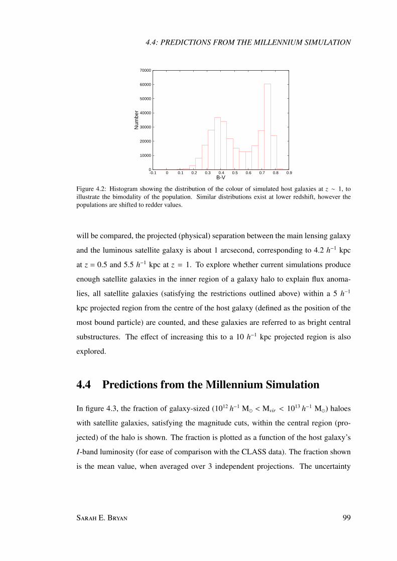
4.4: PREDICTIONS FROM THE MILLENNIUM SIMULATION
0
10000
20000
30000
40000
50000
60000
70000
-0.1 0 0.1 0.2 0.3 0.4 0.5 0.6 0.7 0.8 0.9
Num
ber
B-V
Figure 4.2: Histogram showing the distribution of the colour of simulated host galaxies at z ∼ 1, toillustrate the bimodality of the population. Similar distributions exist at lower redshift, however thepopulations are shifted to redder values.
will be compared, the projected (physical) separation between the main lensing galaxy
and the luminous satellite galaxy is about 1 arcsecond, corresponding to 4.2 h−1 kpc
at z = 0.5 and 5.5 h−1 kpc at z = 1. To explore whether current simulations produce
enough satellite galaxies in the inner region of a galaxy halo to explain flux anoma-
lies, all satellite galaxies (satisfying the restrictions outlined above) within a 5 h−1
kpc projected region from the centre of the host galaxy (defined as the position of the
most bound particle) are counted, and these galaxies are referred to as bright central
substructures. The effect of increasing this to a 10 h−1 kpc projected region is also
explored.
4.4 Predictions from the Millennium Simulation
In figure 4.3, the fraction of galaxy-sized (1012 h−1 M < Mvir < 1013 h−1 M) haloes
with satellite galaxies, satisfying the magnitude cuts, within the central region (pro-
jected) of the halo is shown. The fraction is plotted as a function of the host galaxy’s
I-band luminosity (for ease of comparison with the CLASS data). The fraction shown
is the mean value, when averaged over 3 independent projections. The uncertainty
S E. B 99
4: LUMINOUS SATELLITES IN LENS AND FIELD GALAXIES
corresponds to the Poisson scatter within each bin. The left column shows the fraction
of haloes with bright satellites (MR < −17) within the central 5 h−1 kpc (projected)
while the right column shows the fraction of haloes which contain any (dark or bright)
substructure within the same region. In these plots the red population is depicted using
filled red circles, while the blue population is shown using blue squares. The three
rows show the fraction of haloes containing substructure for the three different red-
shifts considered (top: z = 0, middle: z = 0.5 and bottom: z = 1). Note that the most
luminous blue hosts are not necessarily the most massive haloes but are likely to have
undergone recent star formation.
At z = 0, about 3 − 4% of all of the galaxy-sized haloes appear to have bright
satellite galaxies within 5 h−1 kpc (projected) of the centre of the host. While this
fraction is similar in both types of galaxies, it is found to increase with redshift (rising
to around 11 − 12% at z = 1). Extending the central region to 10 h−1 kpc (not shown),
about 10% of the galaxy-sized haloes host bright central substructure at z = 0, and this
is found to increases to almost 27% at z = 1. If all substructure within the projected
central region is considered, not restricting the search to ‘observable’ satellite galaxies,
the fractions do not change significantly. This is illustrated in the right-hand panels,
where the lower magnitude limits and luminosity ratio cuts have been dropped. The
fraction of haloes containing any substructure within 5 h−1 kpc (projected) of the centre
of the host increases only moderately from ∼ 3% to about 5% at z = 0. This conclusion
remains valid all the way up to z = 1, where the fraction increases from ∼ 11% to about
15%.
Since some of the lensing galaxies reside in groups (see section 4.2), the fraction of
haloes with bright satellites within a projected 5 h−1 kpc region in group-sized haloes
(with 1013 h−1 M ≤ Mvir < 1014 h−1 M) is explicitly checked. The results are shown
in figure 4.4. The fraction of group-sized haloes with bright central substructure is
higher than in galaxy-sized haloes, increasing to ∼ 6% at z = 0 and to ∼ 16% at z = 1
for red galaxies, which dominate the lensing cross-sections; the fraction is slightly
higher for blue galaxies.
100 S D ΛCDM H

4.4: PREDICTIONS FROM THE MILLENNIUM SIMULATION
Table 4.1: Luminosity weighted fraction of galaxy-sized hosts with bright substructure within the central5 h−1 kpc (projected) region. Numbers in brackets correspond to values for group-sized haloes.
Redshift0.0 0.5 1.0
All hosts 3 (6)% 7 (11)% 11 (17)%Red hosts 3 (6)% 6 (11)% 11 (16)%Blue hosts 4 (7)% 7 (16)% 11 (24)%
The lensing cross-section is roughly proportional to σ4 (e.g. Turner et al. 1984),
where σ is the velocity dispersion of the system and, from the Faber-Jackson relation,
L ∝ σ4 for ellipticals (Faber and Jackson 1976). Thus, to compare with observations,
the fraction should be weighted by luminosity. The luminosity weighted fraction of
hosts with bright central substructure is given in table 4.1. At z = 0, the fraction is
∼ 3% for galaxy-sized haloes, increasing to about 6% if only group-sized haloes are
considered. At z = 1, the fraction for galaxy-sized haloes is about 11%, rising to
∼ 17% for group-sized haloes, still below the observed fraction of galaxies with bright
companions (see section 4.2).
Of the systems found to host bright central substructure, most have only one bright
central satellite. Only 2% (3%) of galaxy- (group-) sized hosts with bright central
substructure host more than one bright central satellite at z = 0. At z = 1, 5% (7%) of
galaxy- (group-) sized hosts have multiple bright central satellites. The largest number
of bright central satellites found within any one system is 4.
The force softening of the simulation is 5 h−1 kpc (in comoving coordinates); within
this region, resolution effects may be significant. For this reason, the fraction of the
projected subhaloes within the 3D central region is explicitly checked. The fraction
depends strongly on redshift. About 32% of the luminous satellites found within the
projected central 5 h−1 kpc are found within the 3D central region in galaxy-sized
haloes at z = 0 (for groups this decreases to ∼ 24%). At z = 1 this fraction is 11%,
dropping to ∼ 6% in group-sized haloes (see table 4.2). All of the satellites within the
3D central region are ‘orphan’ galaxies (see section 4.4.1).
Figure 4.5 shows the difference in magnitude between the host and satellite galaxy
S E. B 101

4: LUMINOUS SATELLITES IN LENS AND FIELD GALAXIES
5
10
15
20
25
30
35
40
45
50
10 10.5 11 11.5 12
Hal
oes
with
sub
stru
ctur
e (%
)
log LI ( LO• )
Bright Substructure
R < 5 h-1 kpc
z = 0.0
Red
Blue
5
10
15
20
25
30
35
40
45
50
10 10.5 11 11.5 12
Hal
oes
with
sub
stru
ctur
e (%
)log LI ( LO•
)
Any Substructure
R < 5 h-1 kpc
z = 0.0
Red
Blue
5
10
15
20
25
30
35
40
45
50
10 10.5 11 11.5 12
Hal
oes
with
sub
stru
ctur
e (%
)
log LI ( LO• )
z = 0.5
5
10
15
20
25
30
35
40
45
50
10 10.5 11 11.5 12
Hal
oes
with
sub
stru
ctur
e (%
)
log LI ( LO• )
z = 0.5
5
10
15
20
25
30
35
40
45
50
10 10.5 11 11.5 12
Hal
oes
with
sub
stru
ctur
e (%
)
log LI ( LO• )
z = 1.0
5
10
15
20
25
30
35
40
45
50
10 10.5 11 11.5 12
Hal
oes
with
sub
stru
ctur
e (%
)
log LI ( LO• )
z = 1.0
Figure 4.3: The percentage of galaxy-sized haloes (1012 h−1 M < Mvir < 1013 h−1 M) which havesubstructure within the inner region of the halo, as a function of luminosity L. The left column showsthe fraction of haloes with bright satellites (MR < −17) within the central 5 h−1 kpc (projected) region.The right column shows the fraction of haloes which contain any substructure within the central 5 h−1
kpc (projected) region. In these plots the red population is depicted using filled red circles, while theblue population is shown using blue squares. The three columns show the fraction of haloes containingsubstructure for the three different redshifts considered (top: z = 0.0, middle: z = 0.5 and bottom:z = 1.0). The Poisson scatter is shown. Note that the most luminous blue hosts are not necessarily themost massive haloes but are likely to have undergone recent star formation.
102 S D ΛCDM H
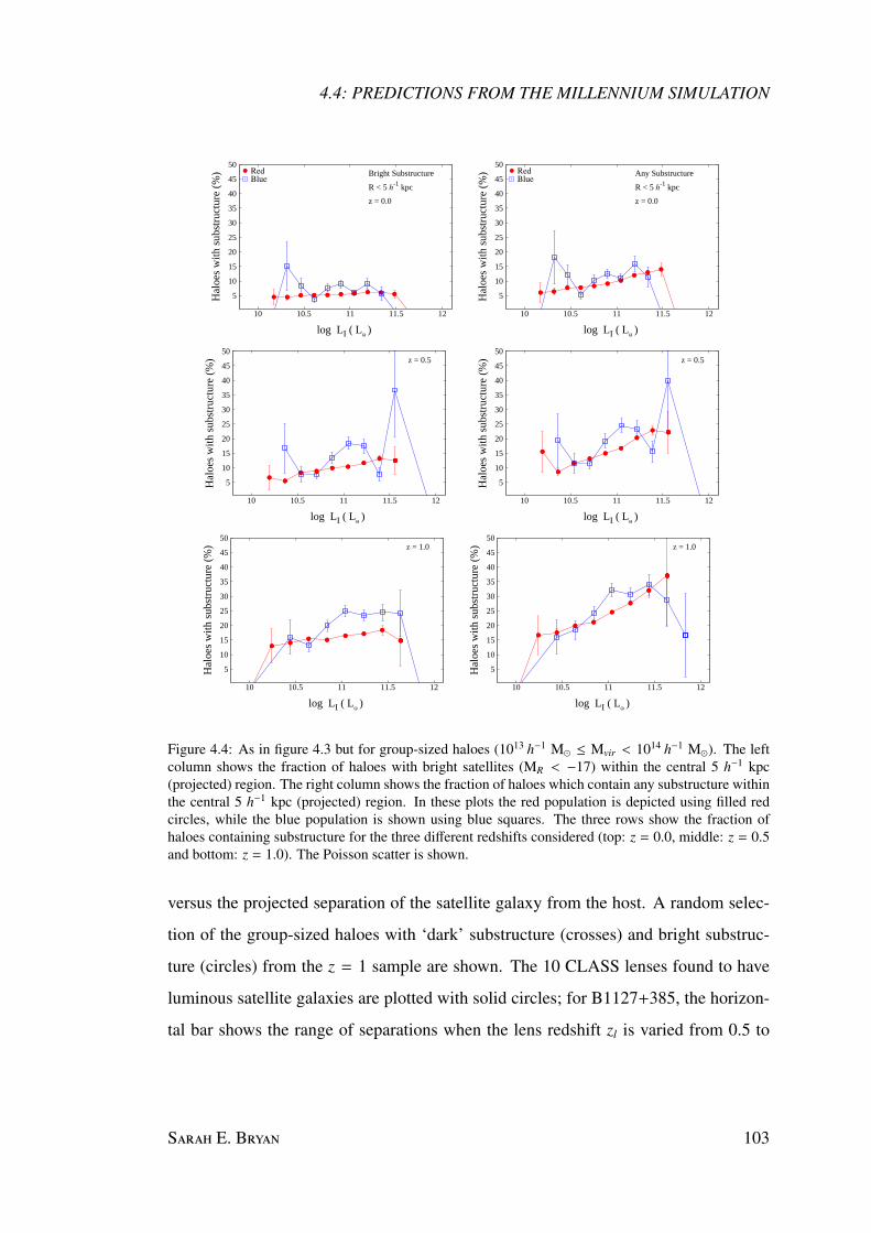
4.4: PREDICTIONS FROM THE MILLENNIUM SIMULATION
5
10
15
20
25
30
35
40
45
50
10 10.5 11 11.5 12
Hal
oes
with
sub
stru
ctur
e (%
)
log LI ( LO• )
Bright Substructure
R < 5 h-1 kpc
z = 0.0
Red
Blue
5
10
15
20
25
30
35
40
45
50
10 10.5 11 11.5 12
Hal
oes
with
sub
stru
ctur
e (%
)
log LI ( LO• )
Any Substructure
R < 5 h-1 kpc
z = 0.0
Red
Blue
5
10
15
20
25
30
35
40
45
50
10 10.5 11 11.5 12
Hal
oes
with
sub
stru
ctur
e (%
)
log LI ( LO• )
z = 0.5
5
10
15
20
25
30
35
40
45
50
10 10.5 11 11.5 12
Hal
oes
with
sub
stru
ctur
e (%
)
log LI ( LO• )
z = 0.5
5
10
15
20
25
30
35
40
45
50
10 10.5 11 11.5 12
Hal
oes
with
sub
stru
ctur
e (%
)
log LI ( LO• )
z = 1.0
5
10
15
20
25
30
35
40
45
50
10 10.5 11 11.5 12
Hal
oes
with
sub
stru
ctur
e (%
)
log LI ( LO• )
z = 1.0
Figure 4.4: As in figure 4.3 but for group-sized haloes (1013 h−1 M ≤ Mvir < 1014 h−1 M). The leftcolumn shows the fraction of haloes with bright satellites (MR < −17) within the central 5 h−1 kpc(projected) region. The right column shows the fraction of haloes which contain any substructure withinthe central 5 h−1 kpc (projected) region. In these plots the red population is depicted using filled redcircles, while the blue population is shown using blue squares. The three rows show the fraction ofhaloes containing substructure for the three different redshifts considered (top: z = 0.0, middle: z = 0.5and bottom: z = 1.0). The Poisson scatter is shown.
versus the projected separation of the satellite galaxy from the host. A random selec-
tion of the group-sized haloes with ‘dark’ substructure (crosses) and bright substruc-
ture (circles) from the z = 1 sample are shown. The 10 CLASS lenses found to have
luminous satellite galaxies are plotted with solid circles; for B1127+385, the horizon-
tal bar shows the range of separations when the lens redshift zl is varied from 0.5 to
S E. B 103

4: LUMINOUS SATELLITES IN LENS AND FIELD GALAXIES
Table 4.2: Fraction of projected central satellites within the 3D central region of galaxy-sized hosts.Numbers in brackets correspond to values for group-sized haloes.
r3D < force softeningz = 0.0 Bright 32 (24)%z = 0.0 Total 26 (17)%z = 0.5 Bright 17 (11)%z = 0.5 Total 14 (8)%z = 1.0 Bright 11 (6)%z = 1.0 Total 9 (5)%
Table 4.3: Percentage of bright satellite galaxies without a surviving dark matter subhalo within thevirial radius and within the central 5 h−1 kpc (projected) region for galaxy-sized hosts. Numbers inbrackets correspond to values for group-sized haloes.
Redshift0.0 0.5 1.0
Satellites without DM subhalo 74 (68)% 81 (76)% 87 (83)%Projected central satellites without DM subhalo 98 (98)% 99 (98)% 99 (99)%
1. Selection effects may be complicated and have not been taken into account in this
study. While it will be difficult to observe satellites with large magnitude differences
at small separations, there are also few simulated satellites found at very small sepa-
rations. (The increase in number with separation is due to the larger area considered.)
As illustrated with the histograms in figure 4.5, the sample of host galaxies and their
luminous satellites considered is comparable to the observed galaxies in the (small)
CLASS sample.
4.4.1 Resolution Effects
As haloes fall into a larger system, they are exposed to tidal forces and are stripped
as they orbit the host system. The extent to which a halo is stripped depends on res-
olution and the inner density profile of the halo (Moore et al. 1996). The simulated
subhaloes have artificially low density cores (due to force softening) that make them
more susceptible to tidal stripping. Including baryons (and gas cooling) will increase
the central density and make the galaxy more resistant to tidal stripping (Moore et al.
1996; Maccio et al. 2006), although the cooling of baryons towards the central host will
104 S D ΛCDM H

4.4: PREDICTIONS FROM THE MILLENNIUM SIMULATION
0
2
4
6
8
10
Dif
fere
nce
in m
agni
tude
1000
0 2 4 6 8 10
Separation (h-1 kpc)
20001000
Figure 4.5: Difference in I-band magnitude between the host and satellite galaxy versus the projectedseparation (in h−1 kpc) of the satellite galaxy from the host. A random selection of the group-sizedhaloes (selected at redshift z = 1.0) with ‘dark’ substructure (crosses) and bright substructure (circles)are shown. The 10 CLASS lenses found to have luminous satellite galaxies are plotted with solid circles;for B1127+385, the horizontal bar shows the range of separations when the lens redshift is varied from0.5 to 1. The histograms show the distribution of bright substructure found within the central 10 h−1 kpc(projected) region as a function of separation and magnitude difference.
also increase the tidal forces experienced by subhaloes that come close to the centre.
Nearly all of the satellite galaxies found in the projected central regions are tidally
stripped ‘orphan’ galaxies (see table 4.3). The semi-analytic model used follows the
orbits of galaxies which have lost their dark matter subhalo, by assuming that they fol-
low the motion of the most bound particle of the parent subhalo before it was destroyed
(this is shown to be a good estimate of the subhalo’s position by Springel et al. 2001a).
Since the effects of dynamical friction on the orbits of these galaxies are not consid-
ered in detail, caution is required when interpreting the results. As noted in Sales et al.
(2007), this may affect the overall abundance and radial distribution of these stripped
haloes.
Also, it is assumed that the ‘orphan’ galaxy remains completely undisturbed for a
merging time, based on the dynamical friction formula of Binney et al. (1987), until
S E. B 105
4: LUMINOUS SATELLITES IN LENS AND FIELD GALAXIES
it merges with the central galaxy. This assumption may result in an over-estimate
of the number of ‘orphan’ galaxies and their associated luminosities. Henriques et al.
(2007) take the opposite approach and assume that all ‘orphan’ galaxies which have not
merged with the central galaxy by z = 0 are completely disrupted, and are responsible
for the diffuse intracluster light. While their results suggest an improved match to the
luminosity function in groups and clusters, the model is simplistic. They note that it
is more likely that the disruption would happen gradually, and that the dense cores
may survive for longer. The extent to which disruption would affect these ‘orphan’
galaxies remains unclear. However, survival of these ‘orphan’ galaxies (at least to some
extent) has been shown by Wang et al. (2006) to be essential in order to explain the
observed correlation signal at small scales. This study used the Millennium Simulation
to construct a new model of galaxy clustering. They found that if ‘orphan’ galaxies
were excluded from the analysis, the correlation signal decreased at small scales in
contrast to observations.
A related question is: if the numerical resolution of the simulation is increased,
would the fraction of luminous satellites rise significantly? Clearly, the number of
subhaloes (dark or luminous) must rise further since the subhalo mass function roughly
follows a power law with dn/dM ∝ M−α, α = 1.7 − 1.9 (Moore et al. 1999; Ghigna
et al. 2000; De Lucia et al. 2004; Gao et al. 2004b; Diemand et al. 2007b). The lowest
mass subhaloes which can be resolved have circular velocities vc at the virial radius
of the order vc . 50 km s−1; haloes with vc . 30 km s−1 may be inhibited from
star formation by the UV background radiation (for example Rees 1986; Efstathiou
1992; Thoul and Weinberg 1996; Gnedin 2000). Thus many subhaloes may remain
dark, and the fraction of bright subhaloes will not increase significantly. Increasing
the resolution of the simulation would also mean that some of the ‘orphan’ galaxies
would be resolved. Since only ‘orphan’ galaxies are allowed to merge with the central
galaxy, increasing the resolution may prolong the lifetime of some of the ‘orphan’
galaxies. To fully understand the impact of this effect a more quantitative analysis
is required. Clearly, a firm conclusion can only be reached using higher-resolution
106 S D ΛCDM H

4.4: PREDICTIONS FROM THE MILLENNIUM SIMULATION
simulations with realistic treatment of the gas processes.
4.4.2 The Effect of Cosmology
The Millennium Simulation assumes a power-spectrum normalisation of σ8 = 0.9,
slightly higher than the latest WMAP seven-year result (Komatsu et al. 2011), where
σ8 = 0.8. A lower value of σ8 will mean that haloes are expected to form later and to
be less concentrated. However, the impact of this parameter on these results is compli-
cated. The semi-analytic models allow some fine-tuning of parameters to match obser-
vations. For example, Wang et al. (2008) found no significant difference in the galaxy
populations (at the redshift range relevant here) created from semi-analytic models
based on the WMAP one-year (Spergel et al. 2003) and WMAP three-year (Spergel
et al. 2007) σ8 values of 0.9 and 0.722, provided suitable galaxy formation parameters
were chosen (the difference becomes significant at high redshift). The results are not
found to change significantly when based on the WMAP3 galaxy catalogue produced
by Wang et al. (2008) when the same merger timescale is adopted (as in their model C).
However, in their model B (which has the same star formation efficiency but a shorter
merger timescale than the De Lucia et al. 2006 catalogue), a factor of ∼ 2 fewer haloes
with central substructure are found.
4.4.3 Comparison with CLASS
Approximately half of the 22 primary lensing galaxies in CLASS appear to have a faint
companion within the projected central 10 h−1 kpc region. The companions have lumi-
nosities of about 2 − 40% of the primary galaxy. Simulated host galaxies covering a
comparable range of luminosities and host-to-satellite separations to the CLASS lenses
have been studied, and the predicted fraction of galaxy- (group-) sized haloes hosting
central luminous satellites (∼ 3% (6%) at z = 0; ∼ 11% (17%) at z = 1) is found to be
lower than the value observed in CLASS. While this fraction is largely independent of
galaxy type, it is shown to increase with redshift.
S E. B 107

4: LUMINOUS SATELLITES IN LENS AND FIELD GALAXIES
Figure 4.6: Cumulative background-subtracted satellite counts for the COSMOS sample using a colourcut of B − V > 0.7 to select elliptical galaxies (figure 6 in Jackson et al. 2010).
The predictions of the redshift and mass dependence appear to be roughly con-
sistent with the data: at least three lenses with luminous satellites are in groups (see
section 4.2), and many appear to have redshifts close to z ∼ 1 , higher than the median
redshift (z ∼ 0.6) of all CLASS lenses (see the bottom panel of figure 4.1).
The comparison so far has not yet considered whether lensing galaxies are biased
tracers of substructure; such bias may arise if substructure enhances the lensing cross-
sections significantly. Previous studies, on cluster scales, for giant arcs indicate that
the bias is small (Hennawi et al. 2007); it remains to be seen whether this holds true
for galaxy-scale lenses. Observationally, SLACS seems to indicate that the lensing
galaxies at z ∼ 0.2 are typical early-type galaxies (Treu et al. 2009).
A natural extension to this study is to compare the predicted frequency with the
observed incidence of bright satellites around elliptical galaxies which are not gravita-
tional lens systems. This is addressed in the next section.
4.5 Satellites in the Field and Lens Galaxies
In Jackson et al. (2010) elliptical galaxies from the COSMOS survey (Capak et al.
2007; Scoville et al. 2007), a 2-square-degree area observed with the Advanced Camera
for Surveys (ACS) on the Hubble Space Telescope (HST) and from the Sloan Digital
108 S D ΛCDM H

4.5: SATELLITES IN THE FIELD AND LENS GALAXIES
Figure 4.7: Cumulative detection rate of SDSS satellites, as a function of secondary/primary flux ratioand linear distance (figure 9 in Jackson et al. 2010).
Figure 4.8: Secondary objects identified in SLACS images within 7 arcseconds of the primary lensover-plotted on the background-subtracted COSMOS counts (figure 11 in Jackson et al. 2010).
Sky Survey (SDSS) data release 7 (Adelman-McCarthy et al. 2008) are used to explore
the observed frequency of companion galaxies around field ellipticals. The CLASS
lenses have also been compared to the SLACS (Bolton et al. 2006, 2008) lens sample,
which uses spectroscopic selection of luminous red galaxies from SDSS observed to
have more than one redshift in their spectra.
For the COSMOS sample, ACS images in the F814W filter were analysed by Neal
Jackson. From this survey 10 974 objects were identified as elliptical galaxies with
photometric redshift greater than 0.1 and I814 magnitude greater than 24.9. The distri-
S E. B 109

4: LUMINOUS SATELLITES IN LENS AND FIELD GALAXIES
0 0.1 0.2 0.3 0.4 0.5 0.6 0.7 0.8 0.9 1
Brightness ratio secondary/primary
Dis
tanc
e/kp
c
5
10
150.
080
0.040
0.02
0
0.010
0.00
5
0.00
2
0.001
0 0.1 0.2 0.3 0.4 0.5 0.6 0.7 0.8 0.9 1
Brightness ratio secondary/primary
Dis
tanc
e/kp
c
5
10
150.200
0.080
0.040
0.0200.010
0.005
0.002
0.001
Figure 4.9: The contours show the proportion of galaxies which contain satellites at less than a certaindistance d and brighter than a flux ratio f , from the primary, using the Millennium Simulation. At eachgrid point, the contoured quantity represents the proportion of primary galaxies which have secondariesat flux ratio f or brighter, at a distance d or closer. The top plot shows the results for all galaxies withz ∼ 0.5 and the bottom plot for z ∼ 1.
110 S D ΛCDM H

4.5: SATELLITES IN THE FIELD AND LENS GALAXIES
butions of redshifts and magnitudes of the COSMOS objects are comparable to those
of CLASS. A spherical region of 11.14 arcseconds (∼ 14 h−1 kpc at z > 0.1) around the
COSMOS objects was searched for secondary objects brighter than I = 24.9. To es-
timate the true frequency of satellites around COSMOS elliptical galaxies, the counts
were corrected to account for chance interlopers. Background counts were established
using 10 000 random positions within the COSMOS survey area. For full details see
Jackson et al. (2010). The background subtracted fraction of elliptical field galaxies
with luminous secondaries identified in the COSMOS sample can be seen in figure 4.6.
The SDSS sample was analysed by Cheng Li. For this sample, all galaxies with r-
band magnitudes r < 18 and spectroscopic redshifts less than 0.5 were considered. The
sample was trimmed to match the redshift and stellar mass distribution of the SLACS
sample, resulting in a sample of 75 839 galaxies. The background subtracted contours
of the average correlated neighbour counts around early-type galaxies can be seen in
figure 4.7.
It is clear that the observed frequency of satellites around field ellipticals is consid-
erably lower than that seen in the CLASS lens galaxies. In order to increase the lens
sample, Neal Jackson analysed the 64 most certain SLACS lenses. Lens candidates are
identified by targeting red galaxies in the SDSS data and searching for systems with
more than one spectroscopic redshift within the ∼ 0.3 arcsecond fibre. SLACS lenses
typically have redshifts between 0.1 and 0.3. A seven arcsecond radius around each
lens galaxy is searched for satellites. A comparison of the COSMOS results with the
lens sample of SLACS is shown in figure 4.8.
The frequency of satellites observed in the field elliptical galaxies within the COS-
MOS sample is consistent with the lower redshift SDSS sample and with that found
in the low redshift lens sample obtained from the SLACS survey (although the lens
sample is still small).
To compare these observations to theoretical predictions from the standard model,
the De Lucia and Blaizot (2007) semi-analytic models run on the Millennium Sim-
ulation were used. Haloes were selected from the galaxy catalogue by imposing a
S E. B 111

4: LUMINOUS SATELLITES IN LENS AND FIELD GALAXIES
minimum mass cut of 1012 h−1 M. All galaxies within these haloes satisfying the
same cutoffs in brightness and colour selection as the observations were considered
(that is, galaxies with magnitudes brighter than I = 24.9 and B − V > 0.7). The virial
radius of each halo was searched for companion galaxies. While previously only cen-
tral galaxies had been considered, all galaxies satisfying the imposed cuts are included
in this analysis. The sample is, however, still dominated by central objects due to the
small number of satellites satisfying the mass cuts.
From figure 4.9 it can be seen that, for the mass range considered, the simulations
give typical satellite fractions of about 8 times those of the COSMOS values, but even
then underpredict the satellite frequency observed in the CLASS samples. The fraction
found in simulations does however depend on the lower mass limit imposed when
selecting host haloes, as higher mass haloes are more likely to host a companion galaxy.
Increasing the mass cut to 1013 h−1 M increases the fraction by a factor of ∼ 2. The
number density of the COSMOS sample can be reproduced by imposing a minimum
halo mass cut of ∼ 3 × 10¹¹ h−1 M (on non-central galaxies); in doing so the fraction
of galaxies found to host a companion is reduced by less than a factor of two (i.e. the
fractions are comparable within the level of uncertainty of the observations).
4.6 Conclusions
Substructure has been proposed to solve the flux anomaly problem, however it remains
unclear as to whether simulations produce enough substructure in the central regions
to account for the observed frequency of this phenomenon. In addition, a closer exam-
ination of the lensing systems reveals that frequently there is an associated luminous
satellite galaxy. The predicted frequency of such luminous satellite galaxies within the
ΛCDM model is considered here.
While ∼50% of the CLASS lens systems appear to have a bright central companion,
the predicted fraction is found to be considerably lower.
Results from the Millennium Simulation combined with semi-analytic galaxy cat-
112 S D ΛCDM H

4.6: CONCLUSIONS
alogues suggest that ∼ 3% (6%) of galaxy- (group-) sized haloes host luminous central
satellites. At z = 1 this fraction is found to be ∼ 11% (17%).
The Poisson probability of detecting luminous substructure in 10 out of 22 lenses,
assuming that 3% of haloes host luminous substructure, is ∼ 2×10⁻⁹. If 17% of haloes
host luminous substructure, the probability of such a detection is ∼ 4 × 10⁻³.
Shin and Evans (2008) recently studied the effect of satellite galaxies on gravi-
tational lensing flux ratios using analytic expressions for the host potential and the
satellite galaxies. They use a spherically symmetric galaxy distribution, and assume
that the three-dimensional number density falls off as r−3.5, comparable to the Milky
Way. They show that the probability of finding a large dwarf is about 10% within two
Einstein radii and about 3% within one Einstein radius. The z = 0 simulation results
are consistent with this.
The predicted frequency is however found to be higher than that observed in the
field galaxies of the COSMOS survey and in the wider, shallower SDSS survey within
the depth and resolution limits of the observations. It is also higher than the fraction
observed in low redshift (z ∼ 0.2) SLACS lenses. The high frequency of satellites seen
in CLASS is anomalous.
When comparing the lens samples, the main difference lies in the median redshift
of the observations. As CLASS lenses are typically at higher redshift than the SLACS
lenses, the redshift evolution predicted by the simulations may help to explain this dis-
crepancy. However, the CLASS lenses and COSMOS field galaxies are drawn from a
similar redshift range. To explain this discrepancy satellites would need to increase the
lensing cross-section enough to bias the lensing statistic. Typically CLASS galaxies
are found to be brighter than their COSMOS counterparts by slightly over a magnitude,
which could be an indication of higher mass haloes. Simulations show that an increase
in halo mass does increase the incidence of close satellites. Increasing the simulated
halo mass of a factor of 10 appears to increase the incidence of close satellites by a
factor of around 2-3. While this may help to reconcile these results, it is unlikely to
increase the fraction sufficiently to completely remove the problem.
S E. B 113

4: LUMINOUS SATELLITES IN LENS AND FIELD GALAXIES
The discrepancy may simply be due to the small number of objects within CLASS.
Another possibility is that some of the luminous ‘satellites’ are not associated with
lensing galaxies at all, but just happen to be along the line of sight (Metcalf 2005).
What is clear from this work is that studying the very central regions of haloes
can provide additional constraints on theoretical models. The central regions are most
sensitive to numerical (resolution) and physical (tidal stripping) effects. Models are
generally able to reproduce the overall luminosity of satellites, but seem unable to
match the small fraction of projected central galaxies.
However, a firm conclusion can only be reached with higher-resolution simulations
involving a realistic treatment of the gas processes. At the same time, a larger sample
of gravitational lenses will also be beneficial to constrain these models and allow more
definitive conclusions on the properties of the substructure to be made.
114 S D ΛCDM H

5
The Impact of Baryons on the Spin
and Shape of Haloes
In this chapter the spin and shape of simulated dark matter haloes extracted from
OWLS are investigated and the effects of baryons and feedback processes on these
properties explored. The spin distributions of the dark matter haloes are well charac-
terised by a log-normal distribution with best-fit values of λ′ = 0.035 and σ = 0.61
in good agreement with previous studies and the angular momentum appears to be
evenly distributed throughout the halo. Dark matter halo shapes are well characterised
by Gaussian functions, with best-fit values for the sphericity of µ = 0.65 and triaxial-
ity of µ = 0.58. The radial dependence of the shapes of dark matter haloes is found
to be weak – massive haloes show a slight decrease in sphericity between 0.06 and
0.25rvir. The triaxiality of the dark matter haloes remains almost constant out to the
virial radius. The sphericity of the dark matter haloes is shown to decrease as a func-
tion of mass while the triaxiality parameter of the halo increases. The overall halo spin
parameter is not strongly affected by the addition of baryons nor by the implemented
feedback prescription, however the spin parameter of the central region (r . 0.12rvir)
of haloes with weak or no feedback is found to be higher than that obtained in the
strong feedback runs. The cooling of baryons acts to make the overall halo mass dis-
S E. B 115

5: THE IMPACT OF BARYONS ON THE SPIN AND SHAPE OF HALOES
tribution more spherical, but stronger feedback prescriptions tend to reduce the impact
of baryons. The distribution of halo sphericity in the dissipational runs is found to be
in broad agreement with observations of elliptical galaxies. The baryonic physics is
shown to have a significant effect on the shape of the dark matter distribution. Weak
stellar feedback runs are able to produce haloes that are almost oblate within the central
regions, while strong stellar and AGN feedback runs result in prolate haloes similar to
those found in dark matter only simulations. The effect of baryons is found to be most
significant in high mass (cluster-scale) haloes.
5.1 Introduction
Dark matter haloes formed in the standard ΛCDM model appear to share a nearly uni-
versal internal morphology (see, for example, Navarro et al. 1996, 1997; Bullock et al.
2001 and Duffy et al. 2008) and are typically thought to be triaxial (Frenk et al. 1988;
Dubinski and Carlberg 1991; Warren et al. 1992; Cole and Lacey 1996; Jing and Suto
2002; Bailin and Steinmetz 2005b; Allgood et al. 2006; Maccio et al. 2006; Bett et al.
2007). Triaxial dark haloes are a natural consequence of hierarchical structure forma-
tion. Smoothed density peaks in the Gaussian random fields that are thought to be the
origin of galaxy collapse in hierarchical models are inherently triaxial (Bardeen et al.
1986). Also, mass accretion onto haloes is thought to be directional, with preferen-
tial infall from associated filaments. Spherical haloes are extremely unlikely in this
formation scenario.
It is also interesting to ask how the shapes of the galaxies embedded within these
dark haloes compare with their hosts. Simulations suggest that including baryons and
considering dissipational processes acts to make the haloes more spherical. It is there-
fore likely that galaxies are also more spherical. However, a direct comparison is
difficult as galaxy formation is a complicated process and the complex interplay be-
tween dissipational cooling and mergers is not fully understood. Disc galaxies are
thought to form in undisturbed systems where the gas is able to cool and condense
116 S D ΛCDM H

5.1: INTRODUCTION
into a rotationally supported disc, while ellipticals are thought to form via dissipation-
less mergers (Toomre 1977). The dissipationless nature of elliptical galaxies makes a
comparison with dark matter haloes a natural analogy. A comprehensive comparison
between theoretical predictions and observations of the angular momentum and the
shapes of galaxies and their dark matter haloes may place important constraints on the
formation processes and the nature of dark matter, thus providing an additional test of
the ΛCDM paradigm.
The angular momentum and shape of a gravitational system are in themselves im-
portant quantities in many respects. For example, misalignment of the angular momen-
tum may cause galactic warps (Ostriker and Binney 1989; Debattista and Sellwood
1999; Bailin and Steinmetz 2005a) or may be responsible for the anisotropic distribu-
tion of haloes (Holmberg 1969 and Knebe et al. 2004). Asphericity in the dark matter
halo will naturally correspond to asphericity in the gas density and will impact on the
shape of X-ray isophotes and the Sunyaev-Zel’dovich signal. Deviations from axisym-
metry in elliptical galaxies may influence the gas kinematics of the system (de Zeeuw
and Franx 1989), and may be responsible for exciting or sustaining warps and stabilis-
ing or deforming polar rings (Steiman-Cameron et al. 1992). Axisymmetry may also
influence the fuelling efficiency of the central black hole (Franx et al. 1991).
The shapes of dark matter haloes are characterised by the axis ratios c/a and b/a
(where a > b > c) of either the density or potential distribution of the halo (denoted
by a subscript ρ or φ, respectively). The sphericity or amount of flattening is described
by c/a while b/a can be used to characterise the elongation of the halo. A spherical
halo has c/a = 1, prolate haloes have two short axes (a >> b ∼ c) and oblate haloes
are characterised by two long axes (a ∼ b >> c). A useful measure of the triaxiality of
a halo is given by T = (a2 − b2)/(a2 − c2), where T = 0 (1) corresponds to an oblate
(prolate) system.
In general, shapes derived from the gravitational potential are more spherical than
S E. B 117

5: THE IMPACT OF BARYONS ON THE SPIN AND SHAPE OF HALOES
those derived from the density distribution . As a general rule of thumb (Sackett 1999):
1 − (c/a)ρ ≈ 3[1 − (c/a)φ
]. (5.1)
In this chapter the spin and shape of haloes are explored using state-of-the-art high-
resolution cosmological hydrodynamical simulations run with different physical pre-
scriptions for the feedback processes. These simulations provide a unique opportunity
to explore the effects of baryons and implemented feedback techniques on a large sam-
ple of haloes evolved within a cosmological setting. The plan of this chapter is as
follows. Section 5.2 reviews current observational estimates of halo shapes and theo-
retical predictions from the literature are discussed in section 5.3. The simulated haloes
used in this analysis are briefly introduced in section 5.4 and the method used to esti-
mate their spin and shape are presented in section 5.5. The spin and shape distributions
of the OWLS dark matter haloes are presented in section 5.6. These are compared to
the baryon runs in section 5.7. Resolution issues are discussed in section 5.8. The halo
shapes are compared to observations of elliptical galaxy shapes in section 5.9 and a
summary of the main results is presented in section 5.10.
5.2 Observational Constraints
There are several methods used to constrain galaxy and halo shapes observationally.
A general review of the techniques used and observational estimates obtained are pre-
sented in Sackett (1999) and constraints on the central density distribution and shape
of the Milky Way’s halo can be found in Merrifield (2004). A useful comparison of
the observational constraints on halo flattening is presented in O’Brien et al. (2010).
A brief summary of these reviews is given here. This summary is by no means an
exhaustive review of the observational constraints but is meant to act as an illustrative
introduction to some of the most common techniques used to estimate halo shapes and
the range of shape parameters thus obtained. A summary of the constraints on the halo
118 S D ΛCDM H

5.2: OBSERVATIONAL CONSTRAINTS
Table 5.1: Observational constraints on (b/a)ρ of haloes, updated from Sackett (1999).
Method System Extent (b/a)ρScatter in Tully-Fisher relation
Franx and de Zeeuw (1992) Spirals HI Gas radius & 0.84Elongation of stellar disc
Lambas et al. (1992) APM survey spirals 1-2 Optical radii & 0.7Fasano et al. (1993) Unbarred RC3 spirals 1-2 Optical radii & 0.8
K-band imaging of face-on systemsRix and Zaritsky (1995) Small HI-linewidths K band radius 0.77 − 0.93
Stellar and gas rotation curvesKuijken and Tremaine (1994) Milky Way 8 - 16 kpc ∼ 0.75
HI gas ring kinematicsFranx et al. (1994) E/SO IC 2006 ∼ 13 kpc 0.96
Analysis of gas kinematicsFranx et al. (1994) E/SO IC 2006 ∼ 13 kpc 0.96Merger remnantsLaw et al. (2009) Milky Way 16 − 60 kpc ≈ 0.83
shapes as described by (b/a) and (c/a) can be found in tables 5.1 and 5.2, respectively.
Elongation
Most observational estimates of the elongation of dark matter density distributions
indicate that (b/a)ρ > 0.7 within the central regions of the halo. Lambas et al. (1992)
and Fasano et al. (1993) use the intrinsic elongation of the stellar disc to estimate the
deviation from axisymmetry of the underlying density distribution. They find that the
stellar distribution in elliptical and early-type spirals is typically triaxial, while the
distribution in spiral galaxies is more axisymmetric. They determine a lower limit of
(b/a)ρ & 0.7 − 0.8. Rix and Zaritsky (1995) used K-band imaging of face on systems
to minimise the effects of dust and spiral structure from young, bright populations, in
an attempt to estimate the non-axisymmetry of the observed potentials. They found
an axis ratio estimate of (b/a)φ ≈ 0.995 corresponding to (b/a)ρ ≈ 0.85. Kuijken
and Tremaine (1994) attempt to resolve the discrepancy between the rotation curve of
the Milky Way derived from stellar and gas tracers assuming that the tracers reside in
different positions in an intrinsically non-axisymmetric potential. Their models lead to
S E. B 119

5: THE IMPACT OF BARYONS ON THE SPIN AND SHAPE OF HALOES
an estimate of (b/a)ρ ≈ 0.75. Observations of the HI gas ring kinematics (Franx et al.
1994) and scatter in the Tully-Fisher relation (Franx and de Zeeuw 1992) also result in
similar constraints on the elongation of the dark matter density distribution. Law et al.
(2009) modelled properties of the Sagittarius tidal stream and found that (b/a)ρ ≈ 0.83
for the Milky Way halo.
Sphericity
Observations of dark matter flattening (c/a or the ratio of vertical to radial axes) are less
consistent. Estimates of the local surface density from stellar kinematics in the solar
neighbourhood result in values of 0.3 < (c/a)ρ < 0.6 (van der Marel 1991; Bienayme
et al. 2006). Amendt and Cuddeford (1994) used measurements of RR Lyrae to probe
the density distribution of the Milky Way out to 60 kpc, and found (c/a)ρ ∼ 0.7.
Estimates of the dark matter distribution from the proper motion of a high-velocity star
(Gnedin et al. 2005) give 0.5 < (c/a)ρ . 1.6.
Gas Flaring. Gas flaring uses the variation of a galaxy’s gas layer with radius to
provide a constraint on the halo shape. Flattening of the dark matter halo will decrease
the tendency for the gas layer to increase with radius. The flaring of HI gas layers is
only able to probe scale heights of a few kpc. Olling (1996) first used this technique to
show that the halo of NGC 4244 was highly flattened with (c/a)ρ ∼ 0.2. A similar flat-
tening is found for NGC 891 by Becquaert and Combes (1997) assuming the gaseous
velocity dispersion to be isotropic. Olling and Merrifield (2000) found that flattenings
of 0.7 < (c/a)ρ < 0.9 were required to fit the observed gas flaring in the Milky Way.
Using the same method O’Brien et al. (2010) find that UGC 7321 has a spherical halo
density distribution with (c/a)ρ ∼ 1.
Tidal Debris. Another probe of the Galaxy’s shape is provided by the tidal debris
of merging satellites. While this approach may extend observational constraints of
the dark matter halo to greater scale heights than the previous methods (the apocentre
120 S D ΛCDM H

5.2: OBSERVATIONAL CONSTRAINTS
Tabl
e5.
2:O
bser
vatio
nalc
onst
rain
tson
(c/a
) ρm
odifi
edan
dup
date
dfr
omSa
cket
t(19
99).
Met
hod
Syst
emE
xten
t( c/a
) ρTr
acer
and
Com
men
tsSt
ella
rkin
emat
ics
Bin
ney
etal
.(19
87)
Milk
yW
ay∼
20kp
c0.
3−
0.8
Pop
IIst
ars
assu
med
totr
ace
over
allk
inem
atic
s.va
nde
rMar
el(1
991)
Milk
yW
ay∼
20kp
c>
0.34
Pop
IIst
ars.
Ass
umes
cons
tant
anis
otro
pylo
cally
and
appr
oxim
ate
hydr
osta
ticeq
uilib
rium
.A
men
dtan
dC
udde
ford
(199
4)M
ilky
Way
<60
kpc
∼0.
7R
RLy
rae
star
s.Te
mpe
ratu
rean
dan
isot
ropy
profi
les
assu
med
tova
ryw
eakl
yw
ithra
dius
.B
iena
yme
etal
.(20
06)
Milk
yW
ay<
1kp
c>
0.5
Red
clum
pst
ars.
Unc
erta
intie
son
extin
ctio
n,di
stan
ces
and
vert
ical
velo
citie
s.R
estr
icte
dsa
mpl
esi
ze.
Hig
hve
loci
tyst
ars
Gne
din
etal
.(20
05)
Milk
yW
ay<
80kp
c0.
5−
1.6
SDSS
J090
745.
0+02
4507
.Lim
ited
sam
ple
size
.Ass
umes
axis
ratio
isco
nsta
ntw
ithra
dius
.G
asfla
ring
few
kpc
Olli
ng(1
996)
NG
C42
440.
1−
0.5
Ver
tical
forc
eba
lanc
edby
grad
ient
sin
ther
mal
pres
sure
.Gas
eous
velo
city
disp
ersi
onel
lipso
idro
und
and
inde
pend
ento
fsca
lehe
ight
.B
ecqu
aert
and
Com
bes
(199
7)N
GC
891
0.2−
0.5
Gas
eous
velo
city
assu
med
tobe
isot
ropi
c.z-
isot
herm
ality
and
axis
ymm
etry
.Gas
and
stel
lars
elf-
grav
ityig
nore
d.O
lling
and
Mer
rifie
ld(2
000)
Milk
yW
ay0.
7−
0.9
HIe
mis
sion
from
gas
inhy
dros
tatic
equi
libri
um.G
asth
ickn
ess
does
notv
ary
azim
utha
lly.D
epen
dson
Gal
actic
cons
tant
s.B
aner
jee
and
Jog
(200
8)M
31∼
0.4
Bul
gean
dda
rkm
atte
rhal
oas
sum
edto
beri
gid
and
non-
resp
onsi
ve.
O’B
rien
etal
.(20
10)
UG
C73
21∼
1G
asve
loci
tydi
sper
sion
isot
herm
alin
z.Ps
eudo
-iso
ther
mal
halo
mod
elas
sum
ed.
Tida
ldeb
ris
ofm
ergi
ngsa
telli
tes
Law
and
Maj
ewsk
i(20
10)
Milk
yW
ay16
<R<
60kp
c∼
0.5
Mod
ellin
gof
the
Sagi
ttari
usst
ream
.MW
mod
elle
das
smoo
thfix
edpo
tent
ial,
disc
assu
med
tolie
onan
axis
ofsy
m.
Pola
rrin
gga
laxi
es5
-20
kpc
Sack
ette
tal.
(199
4)N
GC
4650
A0.
3−
0.4
Ass
umes
gala
xyis
seen
edge
on.
Arn
abol
diet
al.(
1993
)A
M20
20-5
0∼
0.6
Axi
sym
met
ric
mas
sm
odel
.X
-ray
isop
hota
lsha
pes
∼10
-20
kpc
Hyd
rost
atic
equi
libri
umas
sum
ed.
Buo
tean
dC
aniz
ares
(199
6)N
GC
1332
0.28−
0.53
Buo
tean
dC
aniz
ares
(199
7)N
GC
720
0.37−
0.60
Buo
tean
dC
aniz
ares
(199
8)N
GC
3923
0.34−
0.65
Mod
els
ofpr
eces
sing
dust
ydi
scs
Stei
man
-Cam
eron
etal
.(19
92)
NG
C47
53fe
wkp
c0.
84-1
.0G
asor
bits
are
fille
dan
dha
veco
mpl
eted
atle
ast6
orbi
tsat
allr
adii.
Evo
lutio
nof
gase
ous
war
psfe
wkp
cH
ofne
rand
Spar
ke(1
994)
5sp
iral
s0.
6−
0.9
Ass
umes
grav
ityis
the
only
actin
gfo
rce,
radi
alm
ass
flow
and
othe
rdis
sipa
tive
proc
esse
sig
nore
d.N
ewet
al.(
1998
)5
spir
als
>0.
85K
inem
atic
alvi
scos
ityus
edto
sim
ulat
eeff
ecto
fdis
sipa
tive
forc
es.A
ssum
essm
allw
arpsβ
1.St
rong
lens
ing
Ogu
riet
al.(
2003
)38
X-r
aycl
uste
rs-
∼0.
5A
rcst
atis
tics.
Sim
ulat
ions
assu
me
WM
AP
1co
smol
ogic
alpa
ram
eter
san
dsu
bstr
uctu
reis
igno
red.
Ogu
ri(2
010)
SDSS
J100
4+41
12-
∼0.
76C
lust
er-s
cale
quas
arle
nssy
stem
.Mod
elin
clud
espe
rtur
batio
nsfr
omm
embe
rgal
axie
s.K
ocha
nek
(199
5)M
G16
54+
134
-∼
0.3
Ass
umes
anE
inst
ein-
De
Sitte
rmod
el.
Koo
pman
set
al.(
1998
)B
1600
+43
4-
>0.
4E
dge
onsp
iral
gala
xy.
Rus
inet
al.(
2002
)m
ultip
lequ
adle
nssy
stem
s-
>0.
4A
ssum
esa
smoo
thha
lopo
tent
ial,
igno
ring
subs
truc
ture
.Ass
umes
lens
conc
entr
atio
nis
sim
ilart
oth
atof
gene
ralh
aloe
s.C
ohn
and
Koc
hane
k(2
004)
mul
tiple
quad
lens
syst
ems
-∼
0.7
Con
side
rsth
eeff
ecto
fsub
stru
ctur
e.L
ens
mod
elle
das
sing
ular
isot
herm
alsp
here
.W
eak
lens
ing
Ens
embl
eav
erag
edpr
oper
ties.
Proj
ecte
dax
isra
tios.
Hoe
kstr
aet
al.(
2004
)R
ed-S
eque
nce
Clu
ster
Surv
ey-
∼0.
66A
ssum
esha
loal
igne
dw
ithga
laxy
and
ellip
ticity
ofha
lo∝
shap
eof
gala
xy.L
ack
offu
llre
dshi
ftin
form
atio
n.M
ande
lbau
met
al.(
2006
)SD
SSsu
rvey
-∼
0.99
2m
illio
nob
ject
sw
ithph
otom
etri
cre
dshi
fts.
Som
ede
pend
ence
onas
sum
edde
nsity
profi
le.
S E. B 121

5: THE IMPACT OF BARYONS ON THE SPIN AND SHAPE OF HALOES
of Sagittarius is thought to be ∼ 60 kpc), the results are somewhat uncertain. As a
flattened potential would cause the orbit to precess and destroy the observed coherence,
the coherence of the Sagittarius dwarf spheroidal stream over a large angle has been
used to indicate that the inner halo is nearly spherical (Ibata et al. 2001; Fellhauer et al.
2006). However, Johnston et al. (2005) and Martınez-Delgado et al. (2007) argued for
an mildly oblate halo based on a comparison between Sagittarius stream modelling and
2MASS observations of M-stars. Helmi (2004) argued that the data is consistent with
both an oblate and a prolate halo. Helmi questioned whether the observed tracers of
this stream are dynamically old enough to have been significantly affected by the halo
potential. Most recently Law et al. (2009) modelled the Sagittarius stream properties
within a triaxial potential and found that the Milky Way halo within ∼ 60 kpc is triaxial,
with (c/a)ρ ≈ 0.67, (b/a)ρ ≈ 0.83 and T ∼ 0.56.
Polar Ring Galaxies. Polar ring galaxies probe the flattening of the dark halo per-
pendicular to the plane of the disc through comparison of two orthogonal rotation
curves, those of the disc and the inclined ring. This technique probes the halo on
a vertical scale height of between 5 and 20 kpc (Whitmore et al. 1987). Obser-
vations of kinematics in polar ring galaxies show a range of shapes varying from
(c/a)ρ ≈ 0.3 − 0.4 in NGC 4650A (Sackett et al. 1994) to (c/a)ρ ≈ 0.6 in AM2020-50
(Arnaboldi et al. 1993). The dark halo flattening appears to be comparable to, and
aligned with, the stellar system.
X-ray Isophotes. A review of the shapes of elliptical galaxies from X-ray obser-
vations is given in Buote and Canizares (1998). The flattening of extended X-ray
isophotal shapes is used, under the assumption of hydrostatic equilibrium, to provide
a measure of the shape of the gravitational potential in ellipticals, and probes a similar
scale height to the polar ring approach. NGC 720 is found to have 0.37 . (c/a)ρ . 0.60
(Buote and Canizares 1997), a flattening of 0.28 . (c/a)ρ . 0.53 is observed in NGC
1332 (Buote and Canizares 1996) and NGC 3923 is observed to have 0.34 . (c/a)ρ .
122 S D ΛCDM H

5.2: OBSERVATIONAL CONSTRAINTS
0.65 (Buote and Canizares 1998). The inferred axis ratios are comparable to, or smaller
than, those derived from optical observations of the same systems.
Dust Lane Modelling. The complex dust lanes in NGC 4753 were modelled by a
precessing dusty disc by Steiman-Cameron et al. (1992) who found that the flattening
of the system must be modest with (c/a)ρ ≥ 0.84. Estimates of the evolution of warping
in the gas layer also tend to favour modest flattening. Hofner and Sparke (1994) and
New et al. (1998) apply precessing viscous disc models to fit warps observed in five
spiral galaxies (NGC 2841, NGC 3198, NGC 4565, NGC 4013, NGC 4753) finding
that the strength of the quadrupole moment of the underlying dark matter potential
well must be small, implying that the axis ratios would be small. They found that
0.84 . (c/a)ρ . 1.
Gravitational Lensing. Lensing offers a unique probe of a halo potential in that
it provides an estimate of the total mass of the system (baryonic and non-baryonic)
and is not limited to luminous matter. It also does not depend on the dynamical state
of the system. Lenses may, however, be biased since highly elliptical galaxies may
have larger cross-sections. Measuring arc statistics can be used to test the shape of
cluster potentials. Intrinsic ellipticity and substructure can contribute significantly to
the cluster’s ability to form arcs. Oguri et al. (2003) developed a semi-analytic method
for measuring arc statistics, using Monte-Carlo ray tracing simulations based on a
distribution function for the axial ratios drawn from cosmological simulations. They
predicted that triaxial haloes would produce an order of magnitude more arcs than
spherical haloes (the exact differences depend on the density profiles). They compare
their theoretical predictions to a sample of 38 X-ray selected clusters and note that
the triaxial haloes with (c/a)ρ ∼ 0.5 drawn from a ΛCDM cosmology reproduce the
observations well. Kochanek (1995) used the radio ring lens galaxy MG 1654+134
to constrain the central mass and structure of this system. The lens models have axis
ratios of around 0.3 and are always less elliptical than optical estimates of the inner
S E. B 123
5: THE IMPACT OF BARYONS ON THE SPIN AND SHAPE OF HALOES
regions of the lensing galaxy, where the axis ratio is found to be ∼ 0.7. The optical
estimate is based on the innermost regions of the galaxy and a direct comparison is not
possible. A second example of lensing constraints on the shapes of haloes is given by
Koopmans et al. (1998), who studied the edge-on spiral lens B1600+434. The lower
limit on the oblateness of this halo, based on detailed numerical modelling, was found
to be (c/a)ρ ≥ 0.5. The dark matter halo around the lensing galaxy is not as flat as the
luminous stellar (or gas) component. Oguri (2010) analysed the mass distribution of
the cluster-scale quasar lens system SDSS J1004+1422, finding a best-fit axis ratio for
the halo of 0.76. Studies of multiple quad lens systems obtain (c/a)ρ ≥ 0.4 (Rusin
et al. 2002) and (c/a)ρ ∼ 0.7 (Cohn and Kochanek 2004). Weak lensing also provides
a means to probe the mean projected flattening of the dark matter distribution. Studies
by Hoekstra et al. (2004) found 〈c/a〉ρ ∼ 0.66 and (Mandelbaum et al. 2006) measure
〈c/a〉ρ ∼ 0.99 (Mandelbaum et al. 2006) from the SDSS survey.
Concluding Remarks. The different observational methods yield systematically dif-
ferent results for the shapes of dark matter haloes (Olling and Merrifield 2000; O’Brien
et al. 2010). The observations do cover a large range of systems and vary in the extent
of the halo probed, making a direct comparison difficult. Whether the discrepancies re-
sult from halo-to-halo scatter or systematic errors in the observed estimates is unclear.
It is worth noting that Olling and Merrifield (2000) found consistent results for the
flattening of the Milky Way halo (0.7−0.9) using stellar kinematics and the gas flaring
technique. With a rapidly accumulating data set and ever increasing sophistication in
data analysis tools one can soon expect to have a observational data set which may be
more directly compared with theory.
5.3 Theoretical Predictions
Theoretical predictions for halo shapes have been studied extensively. Cold dark matter
models predict triaxial haloes with c/a ∼ 0.6. Hot dark matter models predict spher-
124 S D ΛCDM H

5.3: THEORETICAL PREDICTIONS
ical haloes with c/a ∼ 0.8 (Peebles 1993), while dark matter candidates such as cold
molecular gas and massive decaying neutrinos predict haloes with c/a ∼ 0.2 (Sciama
1990; Pfenniger et al. 1994). Strongly flattened dark matter haloes indicate that the
dark matter is dissipative and possibly baryonic (Sackett et al. 1994). Cosmological
N-body simulations that use the CDM power spectrum (Frenk et al. 1988; Dubinski
and Carlberg 1991) and simulations of an Einstein-de Sitter universe, using a range of
spectral indices (Warren et al. 1992), both produce triaxial haloes.
Early studies of haloes drawn from dissipationless simulations found average (c/a)ρ
values of between 0.5 and 0.8 (Dubinski and Carlberg 1991; Warren et al. 1992; Bul-
lock 2002; Jing and Suto 2002). While Dubinski and Carlberg (1991) and Warren
et al. (1992) obtained (b/a)ρ values in the range 0.4 to 0.9, Bullock (2002) estimated
halo elongations to lie between 0.7 and 1. In these studies the dark matter haloes were
found to be highly flattened and to show a tendency toward prolate shapes (c/b > b/a)
especially in the inner regions. There is disagreement in the literature regarding the ra-
dial dependence of sphericity of simulated haloes. Frenk et al. (1988); Cole and Lacey
(1996); Bullock (2002) and Allgood et al. (2006) note that the sphericity of dark matter
haloes increases with radius while Dubinski and Carlberg (1991); Warren et al. (1992);
Jing and Suto (2002) and Hopkins et al. (2005) suggest that it decreases with radius.
Springel et al. (2004) found that the shape of the dark haloes in dissipationless simula-
tions is nearly constant with radius, noting a weak trend for increased elongation in the
central region. Bailin and Steinmetz (2005b) identified three distinct regions within a
halo; they note that for the most part sphericity increases with radius but that infalling
unvirialised structure at the virial radius results in a decrease in sphericity in the outer
regions of the halo. They also found that the sphericity rises in the innermost regions
(0.06rvir) of their haloes, although they note that this may be a numerical artifact. They
claim that this complicated non-monotonic radial dependence may help to reconcile
the previous results.
Preliminary analyses of galaxy-scale dark matter haloes suggested that they were
systematically rounder than the simulated clusters (Bullock 2002). While there is gen-
S E. B 125
5: THE IMPACT OF BARYONS ON THE SPIN AND SHAPE OF HALOES
eral agreement in the literature that the sphericity of a dark matter halo decreases with
increasing halo mass, the slope of this relation is debated. Bullock (2002) found that
c/a is a strong function of halo mass and decreases from 0.7 for haloes of mass 1012
h−1M to 0.55 for cluster-sized haloes with masses of around 1014 h−1M. Jing and
Suto (2002) found that the sphericity of haloes decreases only slightly with mass.
Springel et al. (2004) and Hopkins et al. (2005) noted a mass dependence similar to
that claimed by Bullock (2002). Maccio et al. (2006) and Bett et al. (2007) found that
the sphericity of the halo ranges from 0.65 to 0.55 over this mass range.
Dissipational simulations predict systematically more spherical haloes than corre-
sponding dissipationless runs (see, for example, Katz and Gunn 1991; Dubinski 1994;
Evrard et al. 1994; Barnes and Hernquist 1996a; Tissera and Dominguez-Tenreiro
1998; Springel et al. 2004; Kazantzidis et al. 2004; Debattista et al. 2008). Gas cooling
is found to increase the axis ratio c/a by > 0.2 in the inner regions; this difference is
found to decrease with radius but appears to persist out to the virial radius.
It is clearly established that the condensation of baryons to the centre of dark matter
haloes tends to result in the halo becoming more spherical or axisymmetric. This result
has been used to explain the discrepancy between the strongly prolate-triaxial shape
found in N-body simulations with the more spherical systems observed. For example,
the distribution of dark matter shapes of haloes drawn from dissipational simulations
is shown to provide a good match to the round stellar systems observed in elliptical
galaxies (Springel et al. 2004).
Clearly a full picture of galaxy formation and evolution requires realistic treatment
of gas processes. However, incorporating baryonic physics in cosmological simula-
tions is a non-trivial task and the computational cost of this process has placed limits
on both the parameter space and the size of the sample of haloes explored to date. The
role of baryons on galaxy formation therefore remains largely uncertain. By provid-
ing identical simulations run with different implementations of the subgrid physics,
OWLS offers a unique opportunity to explore the effects of baryons and implemented
feedback techniques on the spin and shapes of haloes in high-resolution cosmological
126 S D ΛCDM H

5.4: SIMULATIONS AND HALO SAMPLE
simulations.
5.4 Simulations and Halo Sample
The haloes used for this analysis were extracted from OWLS; for detailed information
about these simulations the reader is referred to the discussion in section 3.8.2 and to
Schaye et al. (2010). Here the relevant aspects of the simulations used in this analysis
are briefly reviewed for convenience.
Most of the simulations used in this thesis were run using cosmological parameters
taken from the WMAP3 data as discussed in chapter 3. However, in this chapter, the
effects of cosmology are also considered. This is done by analysing a 5123 particle
dark matter only simulation run with WMAP5 parameters (Komatsu et al. 2009) with:
Ωm = 0.258, ΩΛ = 0.742, h = 0.719, ns = 0.963 and σ8= 0.796. For both of these
cosmologies the dark matter simulations were run in 100 and 400 h−1 Mpc (comoving)
boxes. A smaller simulation run with WMAP1 parameters (Spergel et al. 2003) with:
Ωm = 0.25, ΩΛ = 0.75, h = 0.73, ns = 1 and σ8= 0.9 using 2163 particles in a 50
h−1 Mpc box was also considered (this run has the same resolution as the Millennium
Simulation). In the dark matter only runs the particle mass is 8.6 × 10⁸ h−1 M in the
50 h−1 Mpc box, 4.9× 10⁸ h−1 M in the 100 h−1 Mpc box and 3.1× 10¹⁰ h−1 M in the
400 h−1 Mpc box.
To explore the effect of varying levels of feedback on the shapes and spin param-
eters of haloes extracted from ΛCDM simulations, four baryon runs from the OWLS
simulations are considered. These are summarised in table 3.2 and discussed in detail
in section 3.8.2. Haloes from dark matter only simulations are compared with haloes
in these dissipational hydrodynamic simulations which include gas cooling and star
formation as well as various implementations of feedback (no feedback, weak stellar
feedback, strong stellar feedback and feedback from stars and AGN).
S E. B 127

5: THE IMPACT OF BARYONS ON THE SPIN AND SHAPE OF HALOES
5.5 Methodology
Haloes are defined using the spherical overdensity (SO) approach and all particles
(dark matter and baryonic) within the spherical region are selected for analysis. Four
definitions for the halo outer radius are used in this chapter. Firstly, all particles within
the virial radius rvir are considered, where the mean density is the overdensity ∆ mul-
tiplied by the critical density. Here ∆ is based on the spherical collapse model and
is assumed to depend on cosmology and redshift as described by Bryan and Norman
(1998) (see section 2.2.4). At z = 0, the spherical collapse overdensity ∆ is ∼ 95 for
the cosmological parameters considered here. Haloes defined by r200, r500 and r2500
are also considered, where the mean density is 200, 500 and 2500 times the critical
density respectively. This range of halo definitions probes increasingly smaller and
more central regions of the halo and is chosen to allow for a closer comparison with
observations.
Only haloes that contain more than 1000 particles are considered for this analysis,
as this ensures that the results are fully converged (for a detailed discussion on the
effects of resolution see section 5.8). While estimates of the spin parameter are found
to be well resolved for haloes with more than 300 particles (as in Bett et al. 2007)
a higher number of particles is required to resolve the halo shape (in particular the
triaxiality of the halo). For consistency, the study presented here is therefore limited
to haloes with more than 1000 particles; this conservative limit is in agreement with
that used in Maccio et al. (2008). Haloes are also required to be in a relaxed state
as defined by the centroid shift, that is, the distance between the minimum potential
position (halo centre) and the centre of mass of the halo must be less than 0.07rvir (as
discussed in Neto et al. 2007).
The spin parameters λ′ of the simulated haloes are estimated using the expression
given by Bullock et al. (2001) as
λ′ =J√
2M vc r, (5.2)
128 S D ΛCDM H

5.5: METHODOLOGY
where J is the angular momentum within a sphere of radius r containing mass M and
vc is the halo circular velocity at this radius (v2c = GM (< r) /r). It reduces to the stan-
dard spin parameter (Peebles 1969) when measured at the virial radius of a truncated
singular isothermal halo. For an isolated virialised system, the spin parameter provides
a comparison of the amount of coherent rotation to random motion (Bett et al. 2007).
For a spherical object it can be thought of as the ratio of the object’s angular velocity
to the angular velocity required for rotational support against gravitational collapse.
To characterise the halo shape, the reduced inertia tensor I (weighting particles by
1/r2) is often used such that
Ii j =∑
k
mk
(r2
i δi j − rk,irk, j
)
r2k
, (5.3)
where Ii j are the components of the 3 × 3 inertia tensor. All k particles, each with
mass mk, are summed. The distance of the kth particle from the centre of the halo is
denoted as rk and rk,i is the distance to the i−axis. The mass distribution tensor M(implemented in this work) is also used extensively in the halo shape literature (see,
for example, Cole and Lacey 1996; Bailin and Steinmetz 2005b):
Mi j =∑
k
mkrk,irk, j
r2k
. (5.4)
The square roots of the eigenvalues of the mass distribution tensor, obtained using
Jacobi transformations, are defined as a, b, c (where a > b > c) and are used to measure
the shape of the simulated haloes. Note that the shapes obtained using the inertia tensor
I and the mass distribution tensorM are equivalent (Bett et al. 2007).
As previously mentioned, the shape parameters are defined as follows: s = c/a is
used as a measure of halo sphericity and T = (a2 − b2)/(a2 − c2) as a measure of the
triaxiality of the halo. Computation of the inertia tensor in a spherical region biases
the shapes towards higher sphericity; this is corrected for (as in Bailin and Steinmetz
2005b) by adopting the empirically motivated modified axis ratios (c/a)true ≡ (c/a)√
3measured
S E. B 129
5: THE IMPACT OF BARYONS ON THE SPIN AND SHAPE OF HALOES
and (b/a)true ≡ (b/a)√
3measured. These corrections were calibrated using constructed haloes
with known axis ratios (see Bailin and Steinmetz 2005b).
5.6 Results from a Dissipationless Simulation
In this section, the spin and shape of dark matter haloes are discussed and the effect
of different cosmological models is assessed. The results obtained are compared with
values from the literature.
5.6.1 Spin Distributions
The spin distribution P(λ′) of the 4122 relaxed dark matter haloes (containing more
than 1000 particles) extracted from the WMAP3 simulation at z = 0 is shown in figure
5.1. The left panel shows the distribution of the spin parameter P(λ′) computed within
the virial radius rvir while the right panel shows P(λ′) of the same haloes calculated
using only particles within the central region (0.12rvir). The spin distributions of the
dark matter haloes are well described by a log-normal distribution
P(λ′) =1
λ′√
2πσexp
(− ln(λ′/λ′0)2
2σ2
). (5.5)
with best-fit values of λ′0 = 0.035 and σ = 0.61 when calculated within the virial radius
and λ′0 = 0.038 and σ = 0.63 when computed within the central region. The spin
distribution drawn from these simulations is in excellent agreement with that found by
Bullock et al. (2001) who obtained best-fit values of λ′0 = 0.035 and σ = 0.5, Bailin
and Steinmetz (2005b) who measured λ′0 = 0.035 and σ = 0.58 and Maccio et al.
(2008) who found a mean value of λ′0 = 0.031 and σ = 0.54.
Note that the best-fit values are not substantially different when limiting the analy-
sis to the most central region. As in Bailin and Steinmetz (2005b) the angular momen-
tum appears to be evenly distributed throughout the halo.
The effects of cosmology on the spin parameter distribution of dark matter haloes
130 S D ΛCDM H
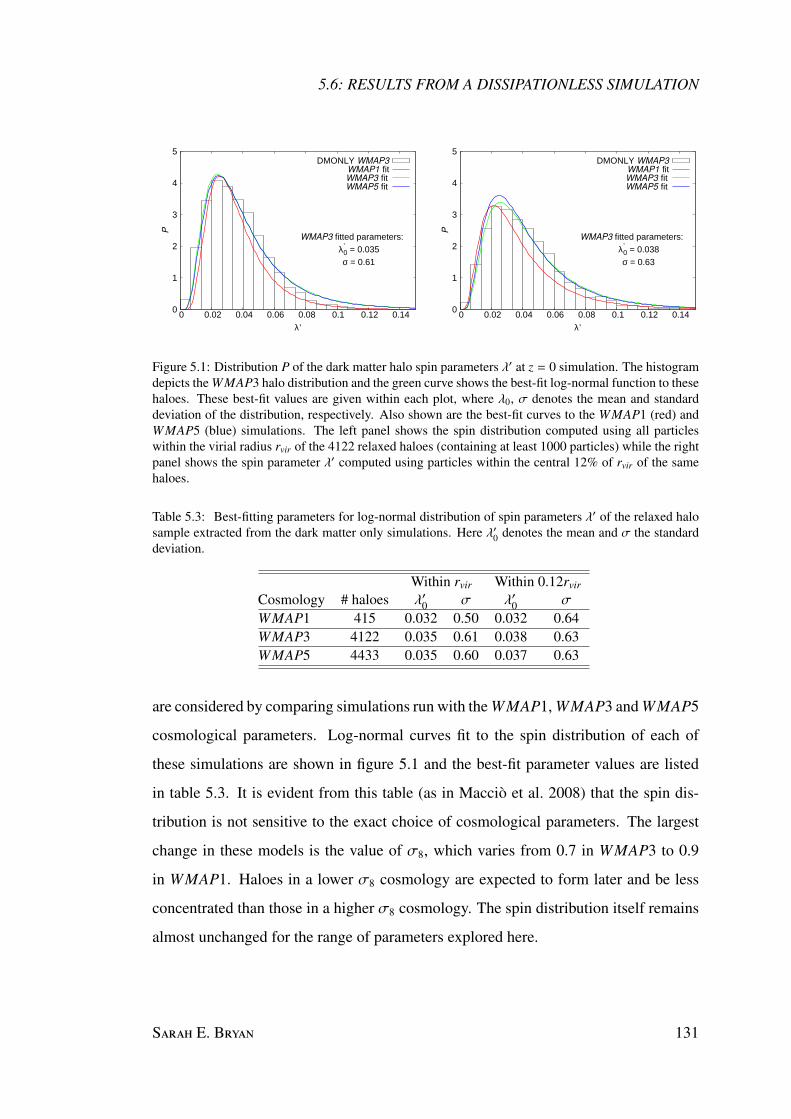
5.6: RESULTS FROM A DISSIPATIONLESS SIMULATION
0
1
2
3
4
5
0 0.02 0.04 0.06 0.08 0.1 0.12 0.14
P
λ’
WMAP3 fitted parameters:λ’
0 = 0.035σ = 0.61
DMONLY WMAP3 WMAP1 fit
WMAP3 fit
WMAP5 fit
0
1
2
3
4
5
0 0.02 0.04 0.06 0.08 0.1 0.12 0.14
P
λ’
WMAP3 fitted parameters:λ’
0 = 0.038σ = 0.63
DMONLY WMAP3 WMAP1 fit
WMAP3 fit
WMAP5 fit
Figure 5.1: Distribution P of the dark matter halo spin parameters λ′ at z = 0 simulation. The histogramdepicts the WMAP3 halo distribution and the green curve shows the best-fit log-normal function to thesehaloes. These best-fit values are given within each plot, where λ0, σ denotes the mean and standarddeviation of the distribution, respectively. Also shown are the best-fit curves to the WMAP1 (red) andWMAP5 (blue) simulations. The left panel shows the spin distribution computed using all particleswithin the virial radius rvir of the 4122 relaxed haloes (containing at least 1000 particles) while the rightpanel shows the spin parameter λ′ computed using particles within the central 12% of rvir of the samehaloes.
Table 5.3: Best-fitting parameters for log-normal distribution of spin parameters λ′ of the relaxed halosample extracted from the dark matter only simulations. Here λ′0 denotes the mean and σ the standarddeviation.
Within rvir Within 0.12rvir
Cosmology # haloes λ′0 σ λ′0 σ
WMAP1 415 0.032 0.50 0.032 0.64WMAP3 4122 0.035 0.61 0.038 0.63WMAP5 4433 0.035 0.60 0.037 0.63
are considered by comparing simulations run with the WMAP1, WMAP3 and WMAP5
cosmological parameters. Log-normal curves fit to the spin distribution of each of
these simulations are shown in figure 5.1 and the best-fit parameter values are listed
in table 5.3. It is evident from this table (as in Maccio et al. 2008) that the spin dis-
tribution is not sensitive to the exact choice of cosmological parameters. The largest
change in these models is the value of σ8, which varies from 0.7 in WMAP3 to 0.9
in WMAP1. Haloes in a lower σ8 cosmology are expected to form later and be less
concentrated than those in a higher σ8 cosmology. The spin distribution itself remains
almost unchanged for the range of parameters explored here.
S E. B 131

5: THE IMPACT OF BARYONS ON THE SPIN AND SHAPE OF HALOES
5.6.2 Shape Distributions
The distributions of the dark matter halo shape parameters can be characterised by a
Gaussian function and are shown in figure 5.2. Histograms are used to illustrate the
shape distribution of haloes from the WMAP3 simulation and the best-fit Gaussian is
shown as a green curve. The top plot presents the distribution of halo sphericity, which
is found to have a best-fit mean value of µ = 0.648 ± 0.002 and standard deviation
σ = 0.098 ± 0.002. The halo elongation distribution, displayed in the central panel,
is characterised by µ = 0.816 ± 0.005 and σ = 0.099 ± 0.005. The distribution of
triaxiality parameters is shown in the bottom plot and is found to have µ = 0.58 ± 0.01
and σ = 0.26± 0.02. Also shown are the fits to the WMAP1 (red) and WMAP5 (blue)
haloes.
5.6.3 Shape Profiles
The radial distribution of the sphericity and triaxiality of dark matter haloes extracted
from the simulations is shown in the left and right panels of figure 5.3, respectively.
The shapes have been computed within cumulative bins. Each row represents a differ-
ent mass range. From top to bottom the mass ranges considered are Mvir < 1012h−1M
(small galaxies), 1012 < Mvir < 1013 h−1 M (large galaxies) and Mvir > 1013 h−1 M
(groups and clusters), respectively. The mass range considered here is comparable
to that explored by Bailin and Steinmetz (2005b). The shapes of haloes taken from
a WMAP1 cosmology are shown as red squares, the shapes of WMAP3 haloes are
shown as green circles and WMAP5 haloes are shown as blue triangles. The error bars
show the 25 and 75 percentiles of the halo-to-halo scatter.
There is no significant difference in either the sphericity or the triaxiality of the
haloes drawn from these three cosmologies. The radial shape profiles of the low mass
haloes are remarkably flat, indicating that the sphericity and triaxiality of these haloes
are constant out to the virial radius, although there is large halo-to-halo scatter in the
triaxiality parameters. The radial dependence of the more massive objects is weak, but
132 S D ΛCDM H
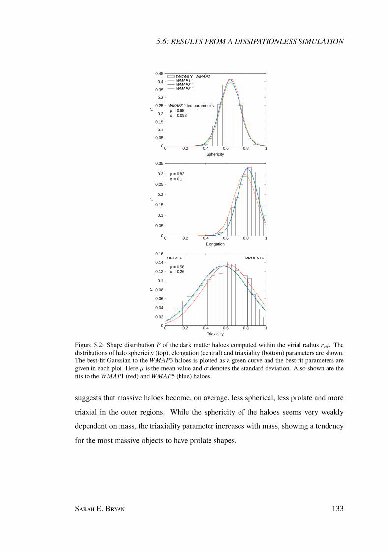
5.6: RESULTS FROM A DISSIPATIONLESS SIMULATION
0
0.05
0.1
0.15
0.2
0.25
0.3
0.35
0.4
0.45
0 0.2 0.4 0.6 0.8 1P
Sphericity
WMAP3 fitted parameters:µ = 0.65σ = 0.098
DMONLY WMAP3
WMAP1 fitWMAP3 fitWMAP5 fit
0
0.05
0.1
0.15
0.2
0.25
0.3
0.35
0 0.2 0.4 0.6 0.8 1
P
Elongation
µ = 0.82σ = 0.1
0
0.02
0.04
0.06
0.08
0.1
0.12
0.14
0.16
0 0.2 0.4 0.6 0.8 1
P
Triaxiality
PROLATEOBLATE
µ = 0.58σ = 0.26
Figure 5.2: Shape distribution P of the dark matter haloes computed within the virial radius rvir. Thedistributions of halo sphericity (top), elongation (central) and triaxiality (bottom) parameters are shown.The best-fit Gaussian to the WMAP3 haloes is plotted as a green curve and the best-fit parameters aregiven in each plot. Here µ is the mean value and σ denotes the standard deviation. Also shown are thefits to the WMAP1 (red) and WMAP5 (blue) haloes.
suggests that massive haloes become, on average, less spherical, less prolate and more
triaxial in the outer regions. While the sphericity of the haloes seems very weakly
dependent on mass, the triaxiality parameter increases with mass, showing a tendency
for the most massive objects to have prolate shapes.
S E. B 133

5: THE IMPACT OF BARYONS ON THE SPIN AND SHAPE OF HALOES
0
0.2
0.4
0.6
0.8
1
0.1 1
Sph
eric
ity
(r / rvir)
Mvir < 1012 h-1MO•
SPHERICAL DMONLY
WMAP1
WMAP3
WMAP5
0
0.2
0.4
0.6
0.8
1
0.1 1
Tria
xial
ity(r / r
vir)
PROLATE
OBLATE
DMONLY
0
0.2
0.4
0.6
0.8
1
0.1 1
Sph
eric
ity
(r / rvir
)
1012 h-1 MO• < M
vir < 1013 h-1M
O•
0
0.2
0.4
0.6
0.8
1
0.1 1
Tria
xial
ity
(r / rvir
)
0
0.2
0.4
0.6
0.8
1
0.1 1
Sph
eric
ity
(r / rvir
)
Mvir
> 1013 h-1 MO•
SPHERICAL
0
0.2
0.4
0.6
0.8
1
0.1 1
Tria
xial
ity
(r / rvir
)
Figure 5.3: The effect of cosmology on the radial shape profiles is explored by comparing dark matteronly simulations run with a WMAP1 (red squares), WMAP3 (green circles) and WMAP5 (blue trian-gles) cosmology. The left panels show the radial distribution of the sphericity of the halo; the rightpanels show the distribution of the triaxiality of the halo. The distributions are plotted in cumulativebins. Each row represents a different mass range (as denoted in the plot). The error bars show the 25and 75 percentiles of the halo-to-halo scatter. The positions of the bins have been staggered for clarity.All bins are beyond the softening range 2.8ε (defined in section 3.2 and discussed in section 3.4.1).
134 S D ΛCDM H

5.6: RESULTS FROM A DISSIPATIONLESS SIMULATION
5.6.4 Shape versus Halo Mass
The relationship between halo shape and mass is shown in figures 5.4 and 5.5. These
figures show the median halo shape (sphericity and triaxiality) within each mass bin
and the error bars show the 25 and 75 percentiles of the halo-to-halo scatter. Haloes are
required to contain at least 1000 particles and mass bins at least 5 haloes. Least-squares
lines of best-fit to each simulation set are also shown and the best-fit values are listed
in table 5.4. This table gives the slope and intercept of the best-fit line, assuming a
pivot mass of Mpivot = 1×10¹² h−1 M. The best-fit line to the sphericity-shape relation
within r200 has a slope of −0.045+0.003−0.007 and an intercept of 0.658+0.005
−0.002 in good agreement
with the values (−0.046 ± 0.016 and 0.630 ± 0.018 ) obtained by Maccio et al. (2008).
Once again, it is clear that there is no significant difference between different cos-
mologies studied here. There is a trend for more massive haloes to be less spherical.
This trend is clear in all cosmologies and for each of the halo definitions considered.
Despite the large halo-to-halo scatter in the triaxiality parameter there is a clear trend
for more massive haloes to have more prolate shapes. This may be a consequence of
their more recent formation time (Springel et al. 2004). The sphericity values com-
puted within rvir vary from 0.66 for haloes of mass 1012 h−1 M to 0.55 for haloes of
mass 1014 h−1 M, in excellent agreement with Maccio et al. (2006) and Bett et al.
(2007). The triaxiality parameter varies from ∼ 0.59 to ∼ 0.73 over the same mass
range. These values are also in agreement with the range of triaxialities (0.68 − 0.8)
found by Bett et al. (2007).
S E. B 135

5: THE IMPACT OF BARYONS ON THE SPIN AND SHAPE OF HALOES
0
0.2
0.4
0.6
0.8
1
-0.5 0 0.5 1 1.5 2 2.5 3
Sph
eric
ity
log ( M / 1012 h-1 MO• )
SPHERICAL
rvir
WMAP1WMAP3WMAP5
0
0.2
0.4
0.6
0.8
1
-0.5 0 0.5 1 1.5 2 2.5 3
Sph
eric
ity
log ( M / 1012 h-1 MO• )
r200
0
0.2
0.4
0.6
0.8
1
-0.5 0 0.5 1 1.5 2 2.5 3
Sph
eric
ity
log ( M / 1012 h-1 MO• )
r500
0
0.2
0.4
0.6
0.8
1
-0.5 0 0.5 1 1.5 2 2.5 3
Sph
eric
ity
log ( M / 1012 h-1 MO• )
r2500
Figure 5.4: Sphericity versus mass M for haloes extracted from dark matter only WMAP1 simulation(red squares), WMAP3 simulations (green circles) and WMAP5 simulations (blue triangles). From leftto right, top to bottom the sphericity is measured within rvir, r200, r500 and r2500. Least-squares linesof best-fit to each simulation set are shown and the best-fit values are listed in table 5.4. Haloes arerequired to contain at least 1000 particles and mass bins are required to contain at least 5 haloes.
136 S D ΛCDM H

5.6: RESULTS FROM A DISSIPATIONLESS SIMULATION
0
0.2
0.4
0.6
0.8
1
-0.5 0 0.5 1 1.5 2 2.5 3
Tria
xial
ity
log ( M / 1012 h-1 MO• )
PROLATE
OBLATE rvir
WMAP1WMAP3WMAP5
0
0.2
0.4
0.6
0.8
1
-0.5 0 0.5 1 1.5 2 2.5 3
Tria
xial
ity
log ( M / 1012 h-1 MO• )
r200
0
0.2
0.4
0.6
0.8
1
-0.5 0 0.5 1 1.5 2 2.5 3
Tria
xial
ity
log ( M / 1012 h-1 MO• )
r500
0
0.2
0.4
0.6
0.8
1
-0.5 0 0.5 1 1.5 2 2.5 3
Tria
xial
ity
log ( M / 1012 h-1 MO• )
r2500
Figure 5.5: As in figure 5.4 but now for triaxiality versus halo mass M.
S E. B 137

5: THE IMPACT OF BARYONS ON THE SPIN AND SHAPE OF HALOES
Table 5.4: Best-fit parameters for the median sphericity and triaxiality of the relaxed halo samplesextracted from a dark matter only simulation run with the WMAP1, WMAP3 and WMAP5 cosmology.The errors correspond to 1σ confidence intervals and have been determined by bootstrap resampling(1000 bootstrap samples have been used).
Sphericity TriaxialitySlope Intercept Slope Intercept
WMAP1rvir −0.076 +0.044
−0.016 0.696 +0.014−0.016 0.037 +0.049
−0.036 0.592 +0.021−0.040
r200 −0.047 +0.023−0.043 0.680 +0.019
−0.008 0.040 +0.059−0.030 0.576 +0.022
−0.031
r500 −0.055 +0.021−0.044 0.678 +0.017
−0.007 0.066 +0.055−0.068 0.602 +0.045
−0.036
r2500 −0.051 +0.020−0.065 0.673 +0.023
−0.016 0.099 +0.211−0.068 0.639 +0.048
−0.073
WMAP3rvir −0.057 +0.006
−0.005 0.676 +0.004−0.004 0.074 +0.005
−0.016 0.586 +0.014−0.005
r200 −0.045 +0.003−0.007 0.658 +0.005
−0.002 0.056 +0.011−0.014 0.611 +0.008
−0.009
r500 −0.039 +0.008−0.006 0.648 +0.004
−0.005 0.058 +0.009−0.007 0.636 +0.009
−0.009
r2500 −0.011 +0.001−0.008 0.635 +0.005
−0.002 0.016 +0.023−0.012 0.720 +0.008
−0.012
WMAP5rvir −0.054 +0.004
−0.003 0.684 +0.003−0.004 0.081 +0.006
−0.008 0.556 +0.011−0.006
r200 −0.051 +0.011−0.004 0.673 +0.003
−0.007 0.075 +0.008−0.013 0.572 +0.014
−0.006
r500 −0.036 +0.004−0.008 0.655 +0.004
−0.003 0.060 +0.005−0.008 0.615 +0.010
−0.006
r2500 −0.025 +0.005−0.004 0.648 +0.004
−0.004 0.019 +0.021−0.025 0.707 +0.010
−0.014
138 S D ΛCDM H

5.7: THE IMPACT OF BARYONS AND FEEDBACK
5.7 The Impact of Baryons and Feedback
This section focuses on the impact of baryons and feedback on the shape and spin of
haloes in a fixed WMAP3 cosmology.
5.7.1 Spin Distributions
The spin distribution of the relaxed haloes (containing more than 1000 particles) ex-
tracted from the WMAP3 baryonic simulations at z = 0 is shown in figure 5.6. The left
panel shows the distribution of the spin parameter computed within the virial radius of
the haloes, while the right panel shows the spin parameter of the same haloes computed
only using particles within the central region (0.12 rvir). This central region is likely
to be more strongly affected by the influence of baryons and feedback. From top to
bottom the spin distribution in the no feedback run (NOFB ZCOOL0), the weak stel-
lar feedback run (REF), the strong stellar feedback run (WDENS) and the stellar and
AGN feedback run (AGN) are shown. The spin distributions are again characterised by
a log-normal distribution, shown as a blue curve with best-fit values given in each plot
(they are also summarised in table 5.5). While the overall spin parameter within rvir
remains unchanged regardless of the type of feedback implemented, the spin parameter
computed within the central region of the weak/no feedback runs is found to be higher
than that seen in the strong feedback runs. The distribution of spin parameters drawn
from the strong feedback runs is comparable to that of the dark matter only haloes. In
the weak feedback runs gas is able to cool dissipatively and condenses in the centre of
the haloes, increasing the central spin of the systems.
5.7.2 Shape Distributions
The distributions of the halo shape parameters are compared to those found in the dark
matter only runs in figure 5.7. The top plot shows the distribution of halo sphericity,
the middle plot shows the distribution of elongation and the distribution of triaxiality
S E. B 139

5: THE IMPACT OF BARYONS ON THE SPIN AND SHAPE OF HALOES
0
1
2
3
4
5
0 0.02 0.04 0.06 0.08 0.1 0.12 0.14
P
λ’
λ’0 = 0.034σ = 0.57
NOFB_ZCOOL0Log-normal fit
0
1
2
3
4
5
0 0.02 0.04 0.06 0.08 0.1 0.12 0.14
P
λ’
λ’0 = 0.048σ = 0.73
NOFB_ZCOOL0Log-normal fit
0
1
2
3
4
5
0 0.02 0.04 0.06 0.08 0.1 0.12 0.14
P
λ’
λ’0 = 0.034σ = 0.58
REFLog-normal fit
0
1
2
3
4
5
0 0.02 0.04 0.06 0.08 0.1 0.12 0.14
P
λ’
λ’0 = 0.046σ = 0.67
REFLog-normal fit
0
1
2
3
4
5
0 0.02 0.04 0.06 0.08 0.1 0.12 0.14
P
λ’
λ’0 = 0.034σ = 0.57
WDENSLog-normal fit
0
1
2
3
4
5
0 0.02 0.04 0.06 0.08 0.1 0.12 0.14
P
λ’
λ’0 = 0.038σ = 0.68
WDENSLog-normal fit
0
1
2
3
4
5
0 0.02 0.04 0.06 0.08 0.1 0.12 0.14
P
λ’
λ’0 = 0.034σ = 0.58
AGNLog-normal fit
0
1
2
3
4
5
0 0.02 0.04 0.06 0.08 0.1 0.12 0.14
P
λ’
λ’0 = 0.037σ = 0.68
AGNLog-normal fit
Figure 5.6: The effect of feedback on the distribution P of the halo spin parameters λ′. From top tobottom the no feedback run (NOFB ZCOOL0), the weak stellar feedback (REF) run, the strong stellarfeedback (WDENS) and the stellar and AGN feedback (AGN) are shown. The curves show the best-fitlog-normal distribution, where the best-fit values are given in the top right corner of each plot. Hereλ′0 denotes the mean and σ the standard deviation. The left panel shows the spin distribution computedusing all particles within the virial radius of the relaxed halo sample while the right panel shows the spinparameter computed using particles within the central 12% of rvir of the same haloes.
140 S D ΛCDM H
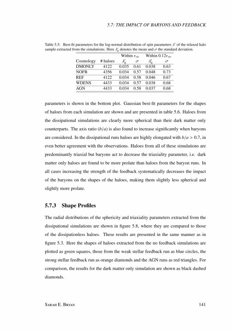
5.7: THE IMPACT OF BARYONS AND FEEDBACK
Table 5.5: Best-fit parameters for the log-normal distribution of spin parameters λ′ of the relaxed halosample extracted from the simulations. Here λ′0 denotes the mean and σ the standard deviation.
Within rvir Within 0.12rvir
Cosmology # haloes λ′0 σ λ′0 σ
DMONLY 4122 0.035 0.61 0.038 0.63NOFB 4356 0.034 0.57 0.048 0.73REF 4122 0.034 0.58 0.046 0.67WDENS 4433 0.034 0.57 0.038 0.68AGN 4433 0.034 0.58 0.037 0.68
parameters is shown in the bottom plot. Gaussian best-fit parameters for the shapes
of haloes from each simulation are shown and are presented in table 5.6. Haloes from
the dissipational simulations are clearly more spherical than their dark matter only
counterparts. The axis ratio (b/a) is also found to increase significantly when baryons
are considered. In the dissipational runs haloes are highly elongated with b/a > 0.7, in
even better agreement with the observations. Haloes from all of these simulations are
predominantly triaxial but baryons act to decrease the triaxiality parameter, i.e. dark
matter only haloes are found to be more prolate than haloes from the baryon runs. In
all cases increasing the strength of the feedback systematically decreases the impact
of the baryons on the shapes of the haloes, making them slightly less spherical and
slightly more prolate.
5.7.3 Shape Profiles
The radial distributions of the sphericity and triaxiality parameters extracted from the
dissipational simulations are shown in figure 5.8, where they are compared to those
of the dissipationless haloes. These results are presented in the same manner as in
figure 5.3. Here the shapes of haloes extracted from the no feedback simulations are
plotted as green squares, those from the weak stellar feedback run as blue circles, the
strong stellar feedback run as orange diamonds and the AGN runs as red triangles. For
comparison, the results for the dark matter only simulation are shown as black dashed
diamonds.
S E. B 141
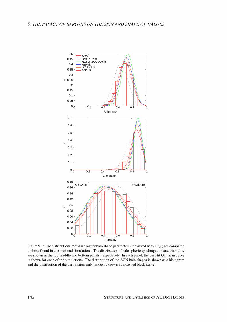
5: THE IMPACT OF BARYONS ON THE SPIN AND SHAPE OF HALOES
0
0.05
0.1
0.15
0.2
0.25
0.3
0.35
0.4
0.45
0.5
0 0.2 0.4 0.6 0.8 1
P
Sphericity
AGNDMONLY fitNOFB_ZCOOL0 fitREF fitWDENS fitAGN fit
0
0.1
0.2
0.3
0.4
0.5
0.6
0.7
0 0.2 0.4 0.6 0.8 1
P
Elongation
0
0.02
0.04
0.06
0.08
0.1
0.12
0.14
0.16
0.18
0 0.2 0.4 0.6 0.8 1
P
Triaxiality
PROLATEOBLATE
Figure 5.7: The distributions P of dark matter halo shape parameters (measured within rvir) are comparedto those found in dissipational simulations. The distribution of halo sphericity, elongation and triaxialityare shown in the top, middle and bottom panels, respectively. In each panel, the best-fit Gaussian curveis shown for each of the simulations. The distribution of the AGN halo shapes is shown as a histogramand the distribution of the dark matter only haloes is shown as a dashed black curve.
142 S D ΛCDM H

5.7: THE IMPACT OF BARYONS AND FEEDBACK
Table 5.6: Best-fit parameters for the Gaussian distribution of halo shape for each of the baryon runs.Here µ denotes the mean value of the distribution and σ the standard deviation.
Simulation µ σ
SphericityDMONLY 0.648 ± 0.002 0.098 ± 0.002NOFB ZCOOL0 0.742 ± 0.001 0.080 ± 0.001REF 0.726 ± 0.002 0.087 ± 0.002WDENS 0.717 ± 0.001 0.088 ± 0.001AGN 0.704 ± 0.002 0.094 ± 0.002
ElongationDMONLY 0.816 ± 0.005 0.099 ± 0.005NOFB ZCOOL0 0.890 ± 0.003 0.055 ± 0.003REF 0.882 ± 0.003 0.057 ± 0.003WDENS 0.875 ± 0.003 0.062 ± 0.003AGN 0.876 ± 0.004 0.070 ± 0.004
TriaxialityDMONLY 0.577 ± 0.013 0.256 ± 0.015NOFB ZCOOL0 0.422 ± 0.008 0.254 ± 0.009REF 0.435 ± 0.008 0.256 ± 0.009WDENS 0.460 ± 0.008 0.256 ± 0.009AGN 0.479 ± 0.011 0.266 ± 0.012
The results in figure 5.8 demonstrate that the effect of baryons is significant out to
the virial radius. The effects of baryons are felt by haloes of all masses, although it is
found to be most significant in the high mass haloes. In the most massive objects there
is a weak trend of decreasing sphericity with increasing radius in the strong feedback
runs; this trend is reduced for the weak feedback runs. In the low mass haloes there is a
slight tendency for haloes to become more spherical at large radii in the weak feedback
runs. Similarly, the strongest effects on triaxiality are found in massive haloes from
simulations with weak or no feedback, and the baryonic physics is found to influence
the halo triaxiality out to the virial radius.
The effects of the dissipational processes on the shape of the dark matter distribu-
tions are shown in figure 5.9, where the halo shape distributions are determined using
only dark matter particles. Again, all of the baryonic runs considered show an increase
in the sphericity and a decrease in the prolateness of the dark matter distribution; these
S E. B 143
5: THE IMPACT OF BARYONS ON THE SPIN AND SHAPE OF HALOES
effects are significant out to rvir but are particularly important in the central regions
of the most massive haloes. Clearly baryons have a significant effect on the shape of
haloes, but these modifications can not be explained solely by the baryon distribution
itself, as the dark matter distribution is also significantly affected.
144 S D ΛCDM H

5.7: THE IMPACT OF BARYONS AND FEEDBACK
0
0.2
0.4
0.6
0.8
1
0.1 1
Sph
eric
ity
(r/rvir)
SPHERICAL DM + BARYONS
Mvir < 1012 h-1 MO•
DMONLYNOFB
REF
WDS
AGN 0
0.2
0.4
0.6
0.8
1
0.1 1
Tria
xial
ity
(r/rvir)
PROLATE
OBLATE
DM + BARYONS
0
0.2
0.4
0.6
0.8
1
0.1 1
Sph
eric
ity
(r/rvir)
1012 h-1 MO• < Mvir < 1013 h-1 M
O•
0
0.2
0.4
0.6
0.8
1
0.1 1
Tria
xial
ity
(r/rvir)
0
0.2
0.4
0.6
0.8
1
0.1 1
Sph
eric
ity
(r/rvir)
Mvir > 1013 h-1MO•
0
0.2
0.4
0.6
0.8
1
0.1 1
Tria
xial
ity
(r/rvir)
Figure 5.8: Effect of feedback on the radial shape profiles. The shapes of haloes extracted from theno feedback (NOFB ZCOOL0) simulation are shown as green squares, those from the weak stellarfeedback run (REF) as blue circles, the strong stellar feedback run (WDENS) as orange diamondsand the AGN runs as red triangles. For comparison the sphericities of dark matter only haloes areshown as black dashed diamonds. The error bars show the 25 and 75 percentiles of the halo-to-haloscatter. The left panels show the radial distribution of the sphericity of the halo; the right panels showthe radial distribution of the triaxiality parameter. The shape parameters are computed in cumulativebins. Each row represents a different mass range. From top to bottom the mass ranges considered areMvir < 1012 h−1 M, 1012 < Mvir < 1013 h−1 M and Mvir > 1013 h−1 M, respectively. All bins are wellbeyond the softening range 2.8ε (defined in section 3.2 and discussed in section 3.4.1).
S E. B 145

5: THE IMPACT OF BARYONS ON THE SPIN AND SHAPE OF HALOES
0
0.2
0.4
0.6
0.8
1
0.1 1
Sph
eric
ity
(r/rvir)
SPHERICAL Only DM
Mvir < 1012 h-1 MO•
DMONLYNOFB
REF
WDS
AGN 0
0.2
0.4
0.6
0.8
1
0.1 1
Tria
xial
ity
(r/rvir)
PROLATE
OBLATE
Only DM
0
0.2
0.4
0.6
0.8
1
0.1 1
Sph
eric
ity
(r/rvir)
1012 h-1 MO• < Mvir < 1013 h-1 M
O•
0
0.2
0.4
0.6
0.8
1
0.1 1
Tria
xial
ity
(r/rvir)
0
0.2
0.4
0.6
0.8
1
0.1 1
Sph
eric
ity
(r/rvir)
Mvir > 1013 h-1 MO•
0
0.2
0.4
0.6
0.8
1
0.1 1
Tria
xial
ity
(r/rvir)
Figure 5.9: As in figure 5.8 but showing the effect of feedback on the radial shape profiles of the darkmatter distribution.
146 S D ΛCDM H
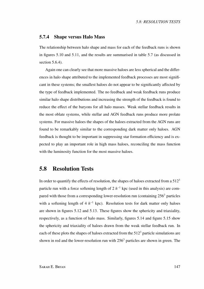
5.8: RESOLUTION TESTS
5.7.4 Shape versus Halo Mass
The relationship between halo shape and mass for each of the feedback runs is shown
in figures 5.10 and 5.11, and the results are summarised in table 5.7 (as discussed in
section 5.6.4).
Again one can clearly see that more massive haloes are less spherical and the differ-
ences in halo shape attributed to the implemented feedback processes are most signifi-
cant in these systems; the smallest haloes do not appear to be significantly affected by
the type of feedback implemented. The no feedback and weak feedback runs produce
similar halo shape distributions and increasing the strength of the feedback is found to
reduce the effect of the baryons for all halo masses. Weak stellar feedback results in
the most oblate systems, while stellar and AGN feedback runs produce more prolate
systems. For massive haloes the shapes of the haloes extracted from the AGN runs are
found to be remarkably similar to the corresponding dark matter only haloes. AGN
feedback is thought to be important in suppressing star formation efficiency and is ex-
pected to play an important role in high mass haloes, reconciling the mass function
with the luminosity function for the most massive haloes.
5.8 Resolution Tests
In order to quantify the effects of resolution, the shapes of haloes extracted from a 5123
particle run with a force softening length of 2 h−1 kpc (used in this analysis) are com-
pared with those from a corresponding lower-resolution run (containing 2563 particles
with a softening length of 4 h−1 kpc). Resolution tests for dark matter only haloes
are shown in figures 5.12 and 5.13. These figures show the sphericity and triaxiality,
respectively, as a function of halo mass. Similarly, figures 5.14 and figure 5.15 show
the sphericity and triaxiality of haloes drawn from the weak stellar feedback run. In
each of these plots the shapes of haloes extracted from the 5123 particle simulations are
shown in red and the lower-resolution run with 2563 particles are shown in green. The
S E. B 147
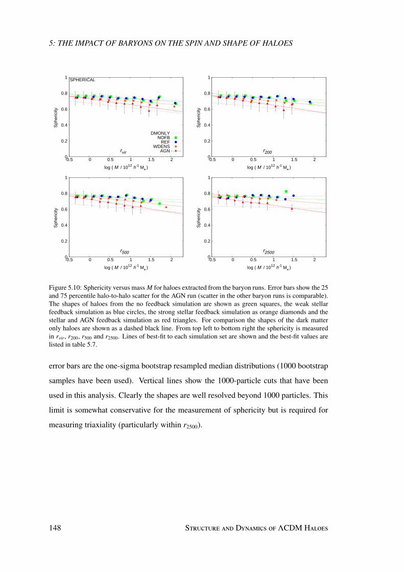
5: THE IMPACT OF BARYONS ON THE SPIN AND SHAPE OF HALOES
0
0.2
0.4
0.6
0.8
1
-0.5 0 0.5 1 1.5 2
Sph
eric
ity
log ( M / 1012 h-1 MO• )
SPHERICAL
rvir
DMONLYNOFB
REFWDENS
AGN 0
0.2
0.4
0.6
0.8
1
-0.5 0 0.5 1 1.5 2
Sph
eric
ity
log ( M / 1012 h-1 MO• )
r200
0
0.2
0.4
0.6
0.8
1
-0.5 0 0.5 1 1.5 2
Sph
eric
ity
log ( M / 1012 h-1 MO• )
r500
0
0.2
0.4
0.6
0.8
1
-0.5 0 0.5 1 1.5 2
Sph
eric
ity
log ( M / 1012 h-1 MO• )
r2500
Figure 5.10: Sphericity versus mass M for haloes extracted from the baryon runs. Error bars show the 25and 75 percentile halo-to-halo scatter for the AGN run (scatter in the other baryon runs is comparable).The shapes of haloes from the no feedback simulation are shown as green squares, the weak stellarfeedback simulation as blue circles, the strong stellar feedback simulation as orange diamonds and thestellar and AGN feedback simulation as red triangles. For comparison the shapes of the dark matteronly haloes are shown as a dashed black line. From top left to bottom right the sphericity is measuredin rvir, r200, r500 and r2500. Lines of best-fit to each simulation set are shown and the best-fit values arelisted in table 5.7.
error bars are the one-sigma bootstrap resampled median distributions (1000 bootstrap
samples have been used). Vertical lines show the 1000-particle cuts that have been
used in this analysis. Clearly the shapes are well resolved beyond 1000 particles. This
limit is somewhat conservative for the measurement of sphericity but is required for
measuring triaxiality (particularly within r2500).
148 S D ΛCDM H

5.8: RESOLUTION TESTS
0
0.2
0.4
0.6
0.8
1
-0.5 0 0.5 1 1.5 2
Tria
xial
ity
log ( M / 1012 h-1 MO• )
PROLATE
OBLATE rvir
0
0.2
0.4
0.6
0.8
1
-0.5 0 0.5 1 1.5 2
Tria
xial
ity
log ( M / 1012 h-1 MO• )
r200
0
0.2
0.4
0.6
0.8
1
-0.5 0 0.5 1 1.5 2
Tria
xial
ity
log ( M / 1012 h-1 MO• )
r500
0
0.2
0.4
0.6
0.8
1
-0.5 0 0.5 1 1.5 2
Tria
xial
ity
log ( M / 1012 h-1 MO• )
r2500
Figure 5.11: As in figure 5.10 but now for triaxiality versus mass of haloes extracted from the baryonruns.
S E. B 149

5: THE IMPACT OF BARYONS ON THE SPIN AND SHAPE OF HALOES
Table 5.7: Best-fit parameters for the median sphericity and triaxiality of the relaxed halo samplesextracted from dissipational simulations. The errors correspond to 1σ confidence intervals and havebeen determined by bootstrap resampling (1000 bootstrap samples have been used).
Sphericity TriaxialitySlope Intercept Slope Intercept
NOFB ZCOOL0rvir −0.036 +0.008
−0.026 0.770 +0.010−0.003 0.064 +0.039
−0.028 0.446 +0.011−0.016
r200 −0.042 +0.016−0.010 0.775 +0.003
−0.006 0.093 +0.037−0.032 0.413 +0.012
−0.013
r500 −0.040 +0.018−0.008 0.776 +0.003
−0.005 0.168 +0.013−0.069 0.377 +0.022
−0.006
r2500 0.018 +0.001−0.030 0.763 +0.007
−0.001 0.065 +0.077−0.016 0.412 +0.010
−0.015
REFrvir −0.022 +0.010
−0.022 0.754 +0.008−0.005 0.044 +0.039
−0.026 0.447 +0.014−0.015
r200 −0.021 +0.009−0.018 0.760 +0.007
−0.004 0.070 +0.038−0.052 0.411 +0.018
−0.015
r500 −0.019 +0.010−0.013 0.763 +0.004
−0.004 0.112 +0.063−0.054 0.376 +0.013
−0.024
r2500 0.006 +0.021−0.008 0.754 +0.003
−0.004 0.165 +0.033−0.037 0.307 +0.007
−0.012
WDENSrvir −0.041 +0.011
−0.017 0.744 +0.006−0.005 0.077 +0.027
−0.035 0.477 +0.014−0.009
r200 −0.046 +0.018−0.010 0.747 +0.004
−0.006 0.086 +0.042−0.035 0.456 +0.012
−0.014
r500 −0.054 +0.020−0.010 0.758 +0.004
−0.007 0.153 +0.037−0.077 0.425 +0.015
−0.017
r2500 −0.043 +0.018−0.007 0.768 +0.003
−0.004 0.175 +0.026−0.120 0.403 +0.025
−0.006
AGNrvir −0.071 +0.013
−0.018 0.730 +0.006−0.006 0.176 +−0.001
−0.056 0.485 +0.018−0.003
r200 −0.077 +0.024−0.008 0.729 +0.002
−0.009 0.172 +0.018−0.069 0.484 +0.021
−0.007
r500 −0.081 +0.028−0.006 0.727 +0.002
−0.007 0.176 +0.028−0.056 0.486 +0.018
−0.009
r2500 −0.072 +0.025−0.000 0.722 +0.003
−0.004 0.144 +0.074−0.067 0.549 +0.010
−0.019
150 S D ΛCDM H
5.8: RESOLUTION TESTS
0
0.2
0.4
0.6
0.8
1
-1 -0.5 0 0.5 1 1.5 2 2.5
Sph
eric
ity
log ( M / 1012 h-1 MO• )
rvir
SPHERICALL100N512L100N256
0
0.2
0.4
0.6
0.8
1
-1 -0.5 0 0.5 1 1.5 2 2.5
Sph
eric
ity
log ( M / 1012 h-1 MO• )
r200
0
0.2
0.4
0.6
0.8
1
-1 -0.5 0 0.5 1 1.5 2 2.5
Sph
eric
ity
log ( M / 1012 h-1 MO• )
r500 0
0.2
0.4
0.6
0.8
1
-1 -0.5 0 0.5 1 1.5 2 2.5
Sph
eric
ity
log ( M / 1012 h-1 MO• )
r2500
Figure 5.12: The effect of resolution on the sphericity of simulated dark matter only haloes at z = 0.The shapes of haloes extracted from the 5123 particle simulations are shown in red while those fromthe lower resolution 2563 particle run are shown in green. The errors correspond to 1σ confidenceintervals and have been determined by bootstrap resampling (1000 bootstrap samples have been used).Vertical lines correspond to a 1000-particle cut for each of the simulations considered, only haloes withmasses greater than this limit are considered for analysis. From top left to bottom right the sphericity ismeasured within rvir, r200, r500, r2500.
S E. B 151

5: THE IMPACT OF BARYONS ON THE SPIN AND SHAPE OF HALOES
0
0.2
0.4
0.6
0.8
1
-1 -0.5 0 0.5 1 1.5 2 2.5
Tria
xial
ity
log ( M / 1012 h-1 MO• )
rvir
PROLATE
OBLATE
L100N512L100N256
0
0.2
0.4
0.6
0.8
1
-1 -0.5 0 0.5 1 1.5 2 2.5
Tria
xial
ity
log ( M / 1012 h-1 MO• )
r200
0
0.2
0.4
0.6
0.8
1
-1 -0.5 0 0.5 1 1.5 2 2.5
Tria
xial
ity
log ( M / 1012 h-1 MO• )
r500 0
0.2
0.4
0.6
0.8
1
-1 -0.5 0 0.5 1 1.5 2 2.5
Tria
xial
ity
log ( M / 1012 h-1 MO• )
r2500
Figure 5.13: As in figure 5.12 but for the triaxiality of the dark matter only haloes.
152 S D ΛCDM H

5.8: RESOLUTION TESTS
0
0.2
0.4
0.6
0.8
1
-1 -0.5 0 0.5 1 1.5 2 2.5
Sph
eric
ity
log ( M / 1012 h-1 MO• )
rrvir
SPHERICALL100N512L100N256
0
0.2
0.4
0.6
0.8
1
-1 -0.5 0 0.5 1 1.5 2 2.5
Sph
eric
ity
log ( M / 1012 h-1 MO• )
r200
0
0.2
0.4
0.6
0.8
1
-1 -0.5 0 0.5 1 1.5 2 2.5
Sph
eric
ity
log ( M / 1012 h-1 MO• )
r500 0
0.2
0.4
0.6
0.8
1
-1 -0.5 0 0.5 1 1.5 2 2.5
Sph
eric
ity
log ( M / 1012 h-1 MO• )
r2500
Figure 5.14: The effect of resolution on the sphericity of haloes from a weak stellar feedback simulation(REF) at z = 0. The shapes of haloes extracted from the 5123 particle simulations are shown in red whilethe shapes of haloes from the lower resolution 2563 particle run are shown in green. The errors corre-spond to 1σ confidence intervals and have been determined by bootstrap resampling (1000 bootstrapsamples have been used). Vertical lines correspond to a 1000-particle cut for each of the simulationsconsidered, only haloes with masses greater than this limit are considered for analysis. From top left tobottom right the triaxiality is measured within rvir, r200, r500, r2500.
S E. B 153

5: THE IMPACT OF BARYONS ON THE SPIN AND SHAPE OF HALOES
0
0.2
0.4
0.6
0.8
1
-1 -0.5 0 0.5 1 1.5 2 2.5
Tria
xial
ity
log ( M / 1012 h-1 MO• )
rvir
PROLATE
OBLATE
L100N512L100N256
0
0.2
0.4
0.6
0.8
1
-1 -0.5 0 0.5 1 1.5 2 2.5
Tria
xial
ity
log ( M / 1012 h-1 MO• )
r200
0
0.2
0.4
0.6
0.8
1
-1 -0.5 0 0.5 1 1.5 2 2.5
Tria
xial
ity
log ( M / 1012 h-1 MO• )
r500 0
0.2
0.4
0.6
0.8
1
-1 -0.5 0 0.5 1 1.5 2 2.5
Tria
xial
ity
log ( M / 1012 h-1 MO• )
r2500
Figure 5.15: As in figure 5.14 but for the triaxiality of the weak feedback (REF) haloes.
154 S D ΛCDM H

5.9: COMPARISON TO SHAPES OF ELLIPTICAL GALAXIES
5.9 Comparison to Shapes of Elliptical Galaxies
In figure 5.16 the (c/a) ≡ γ and (b/a) ≡ β axis ratios are compared to the observational
estimates of Ryden (1992) (shown as a red curve). They used a sample of 171 elliptical
galaxies to constrain the intrinsic axis ratios, finding that Gaussian distributions with
means µγ = 0.69, µβ = 0.98 and standard deviations σγ = 0.11, σβ = 0.11 provided
good fits to the observations of (c/a) and (b/a) axis ratios, respectively. Similarly,
Lambas et al. (1992) studied 3165 elliptical galaxies from the APM Bright Galaxy
Survey, finding that the best-fit values for the distribution of axial ratios of the elliptical
galaxies were µγ = 0.55, σγ = 0.2 and µβ = 0.95, σβ = 0.35. Kimm and Yi (2007) use
the SDSS data release 5 to estimate the axis ratios of a volume-limited sample of 3922
early-type galaxies at 0.05 ≤ z ≤ 0.06. This data is well fit by Gaussian distributions
with values of µγ = 0.78, σγ = 0.3 and µβ = 0.92, σβ = 0.1, in agreement with Ryden
(1992).
Figure 5.16 shows the distribution of axis ratios of dark matter haloes in blue and
of haloes with baryons, cooling and no feedback, in pink (NOFB ZCOOL0). These re-
sults bracket the range of shapes observed in the simulations. The axis ratios estimated
from Ryden (1992) are shown in red. In the left panel the (c/a) axis ratios are com-
pared to the distribution found by Dubinski (1994) for dark matter haloes (in green).
The right panel shows the (b/a) axis ratios. Dubinski (1994) found that the (b/a) of
dark matter haloes was ∼ 0.5 but that this increased to ∼ 0.7 − 0.8 when baryons were
included. In this plot the green curve shows the observational estimates of Kimm and
Yi (2007). While the distribution of the axis ratios is fairly broad, the distributions
predicted by dissipational simulations seem to be in agreement with the observations
of elliptical galaxies.
S E. B 155

5: THE IMPACT OF BARYONS ON THE SPIN AND SHAPE OF HALOES
0
2
4
6
8
10
12
14
0 0.2 0.4 0.6 0.8 1
P
Sphericity
Ryden 1992Dubinski 1994DMONLYNOFB_ZCOOL0AGN
0
2
4
6
8
10
12
14
0.5 0.6 0.7 0.8 0.9 1
P
Elongation
Ryden 1992Kimm 2007DMONLYNOFB_ZCOOL0AGN
Figure 5.16: Comparison of the shape distributions P with observations. The left panel shows thedistribution (c/a) while (b/a) is shown on the right. The shapes simulated haloes from the no feedback(dark matter) run are shown in pink (blue) while those from the AGN simulation are shown as a dashedblack curve. The observed samples used for comparison can be seen in the key and are discussed in thetext.
5.10 Summary
The spin and shape distribution of haloes are characteristic of the paradigm in which
they form and evolve. In this chapter the spin distribution and shape of dark matter
haloes are explored and compared with simulations which include hydrodynamical
treatment of baryonic physics such as gas cooling, star formation and feedback.
The spin parameter of relaxed dark matter haloes is characterised by a log-normal
curve with best-fit values of λ′0 = 0.035 and σ = 0.61 in excellent agreement with
Bullock et al. (2001); Bailin and Steinmetz (2005b) and Maccio et al. (2008). The spin
distribution is remarkably similar in a WMAP1, WMAP3 and WMAP5 cosmology.
This result suggests that there is no strong redshift dependence as the variation in σ8
explored by these simulations results in different halo formation times: haloes in the
lower σ8 (WMAP3) simulation are expected to form later than those in the higher
σ8 (WMAP1) simulation. The angular momentum of dark matter haloes appears to
be evenly distributed throughout the halo and the spin parameter remains essentially
unchanged if computed using only mass within the central region (0.12rvir), as found
by Bailin and Steinmetz (2005b).
The spin distribution of haloes extracted from the baryon runs is not significantly
156 S D ΛCDM H

5.10: SUMMARY
different to that of dark matter only haloes when computed using all mass within rvir.
However, in the central regions where baryons are expected to dominate, haloes from
weak feedback simulations tend to have higher mean spin values than those from strong
feedback runs. The spin distribution in the central region of strong feedback simula-
tions is comparable to the distribution found for dark matter only haloes.
Dark matter only haloes extracted from OWLS typically have sphericities of ∼ 0.55
to 0.7 and triaxialities of between 0.55 and 0.8 (indicating triaxial to prolate shapes).
The choice of cosmological parameters does not significantly affect the shape of the
simulated haloes (consistent with Maccio et al. 2006). Again, as the halo shape is not
particularly sensitive to the choice of σ8; this suggests that the redshift evolution of the
shape of haloes is weak.
The radial shape profiles of low mass dark matter halo shapes are remarkably flat,
indicating that the halo shape is essentially constant out to the virial radius (as found
in Springel et al. 2004). There is a weak radial trend in the triaxiality parameters
of massive haloes, indicating that these haloes become less prolate and more triaxial
towards rvir. More massive haloes are found to be less spherical and more prolate than
lower mass haloes, in agreement with Maccio et al. (2006) and Bett et al. (2007).
It is well established that dissipational simulations tend to produce more spheri-
cal haloes than corresponding dissipationless runs (see, for example, Katz and Gunn
1991; Evrard et al. 1994; Tissera and Dominguez-Tenreiro 1998; Kazantzidis et al.
2004; Springel et al. 2004; Debattista et al. 2008) due to the presence of isotropic gas
pressure. It is thought that baryons act to influence the orbital content of the halo,
decreasing the fraction of box orbits responsible for supporting the triaxial halo (see
chapter 6). In all of the OWLS runs considered, baryons act to make the haloes more
spherical, although the stronger the feedback prescription the smaller the impact on the
halo shape. Weak stellar feedback runs are able to produce almost oblate haloes, while
stellar and AGN feedback runs result in prolate haloes similar to those found in dark
matter only simulations. The effect of baryons is found to be most significant in high
mass haloes. Baryons are also shown to have a significant effect on the shape of the
S E. B 157

5: THE IMPACT OF BARYONS ON THE SPIN AND SHAPE OF HALOES
dark matter distribution, i.e. the results cannot solely be attributed to the shape of the
baryon distribution itself.
Finally, the shapes of the dark matter haloes taken from the OWLS simulations are
found to be in agreement with a wide range of observational estimates of the shapes of
elliptical galaxies.
158 S D ΛCDM H
6
The Effect of Feedback on the Orbital
Content of Haloes
In this chapter, the orbital content of a large sample of haloes extracted from state-of-
the-art high-resolution cosmological hydrodynamical simulations has been explored.
The effects of the feedback prescriptions on the dynamics and orbits of the dark matter
particles, stellar particles and subhaloes are quantified through spectral analyses of
their orbits. The inner region (0.25r200) of dark matter haloes is found to be dominated
by box orbits. However, adding baryons to these simulations results in a decrease in the
fraction of central box orbits. Increasing the strength of the feedback implementation
is found to reduce the central concentration of baryons, and correspondingly results in
an increase in the fraction of box orbits. The orbital content described by the stellar
particles is found to be remarkably similar to that drawn from the orbits of dark matter
particles. How the orbital content of the haloes depends on several key parameters such
as their mass, redshift and dynamical state is also considered. The results presented
in this chapter may be used as constraints for dynamical modelling of galaxies using
Schwarzschild’s or Made-to-Measure methods.
S E. B 159

6: THE EFFECT OF FEEDBACK ON THE ORBITAL CONTENT OF HALOES
6.1 Introduction
Studying the dynamics of a halo provides an unparallelled view of its internal kinemat-
ics and affords the opportunity to infer its basic properties. Studying the orbital content
of haloes may also provide dynamical information about the halo’s formation history.
The Gaia satellite, to be launched in 2012, will provide a kinematic census of our
Galaxy. In order to fully exploit observational datasets such as this, a comprehensive
comparison with simulations is essential.
Stellar systems, such as elliptical galaxies, are fully described by their distribution
function or density in 6D phase space. All of the galaxy’s photometric and kinematic
properties can be thought of as a superposition of the underlying orbits within the
galaxy. Approaches such as Schwarzschild’s method (Schwarzschild 1979) and Made-
to-Measure techniques (Syer and Tremaine 1996; de Lorenzi et al. 2007; Dehnen 2009;
Long and Mao 2010) attempt to reproduce observables using a superposition of the or-
bital density distributions. While in many cases, these techniques are able to reproduce
a number of observables, the chosen orbital distribution may not be unique. It is pos-
sible that different combinations of orbits with distinctly different shapes may produce
the same triaxial density distribution (de Zeeuw and Franx 1991). Studying the orbital
content of merger remnants provides a unique insight into the types of orbital distri-
butions expected to be present in galaxies with specified properties, and may help to
provide initial conditions for these methods.
Orbits are divided into groups, or families, according to the phase space they cover.
Families of regular orbits have similar morphologies because they conserve similar in-
tegrals of motion. These isolating integrals restrict the region of phase space available
to an orbit. Each lowers, by one, the dimensionality of the region available to the orbit.
As such, an orbit is shaped by its isolating integrals. Axisymmetric potentials have two
classical integrals of motion: energy E and the z-component of the angular momen-
tum Lz, it has been shown that a third non-classical integral is required to understand
the dynamics of the solar neighbourhood (Lindblad 1933; Contopoulos 1960; Binney
160 S D ΛCDM H

6.1: INTRODUCTION
and Spergel 1982). However, it is well-known that many elliptical galaxies are not
axisymmetric (Franx et al. 1991). In more relevant triaxial systems, there are two non-
classical integral that play a fundamental role in shaping the system (Schwarzschild
1979).
Within simple generic triaxial models, regular orbits can be divided into two main
families: box and tube orbits. Tube orbits are further divided according to their ori-
entation into major- and minor-axis tubes (Schwarzschild 1979; Statler 1987). Box
orbits are free to pass close to the centre of the potential and their orbit-averaged an-
gular momentum is zero. While box orbits show no sense of rotation, tube orbits tend
to rotate around the centre of the system, avoiding the centre. Studying the orbital
families allows us to use the orbital structure of the galaxy to infer information about
its formation history.
Box orbits are fundamentally important, as they are thought to be responsible for
conveying information from the central regions of a halo to the outer parts of the system
and are required to support the triaxial halo. It has been proposed that the decrease in
triaxiality of dark matter haloes experienced when baryons are included is due to the
scattering of these box orbits (see, for example, Debattista et al. 2008). Any central
concentration (such as gas cooling and settling to the centre of the potential or massive
black hole growth) is likely to affect the box orbits. Altering the distribution of the
orbits can modify the shape of the halo. Scattering of the box orbits is likely to make
the halo rounder and more oblate (Gerhard and Binney 1985). It is interesting to ask
what kind of orbits are possible within a given potential, and how these orbits are
modified when the potential is altered. These questions are addressed in this chapter.
Several authors have investigated the orbital content of analytic potentials and rem-
nants of simulated disc mergers. The first attempt to classify the orbital content of
simulated merger remnants was conducted by Barnes (1992) who simulated a small
sample of merging encounters between equal mass disc galaxies with varying disc ori-
entations and impact parameters. Orbits were classified using a ‘spin classification
routine’, based on changes in the sign of the angular momentum vector. The merger
S E. B 161

6: THE EFFECT OF FEEDBACK ON THE ORBITAL CONTENT OF HALOES
remnants were found to exhibit a wide variety of shapes and orbital structure. The
remnants’ shapes and kinematic properties were found to be related to the initial disc
spin vectors and other encounter parameters. Almost all of the most tightly bound par-
ticles were found to be on box orbits and, further out, minor-axis tube orbits dominated
the merger remnant. In major mergers (where the masses of the progenitor haloes are
comparable) the violent merging process tends to result in a remnant largely dominated
by box orbits. During minor mergers, the disc component is not destroyed and tube
orbits remain. Barnes (1992) argues that most ellipticals cannot have formed by stellar
dynamical mergers of equal-mass galaxies since significant misalignment between the
minor and rotation axes was found in many of the merger remnants.
By including gas dynamics in the merging galaxies, Barnes and Hernquist (1996b)
showed that gas tends to accelerate the orbital decay slightly, and that it can have a
dramatic effect on the structure of the resulting remnant. Torques experienced during
the merger act to remove angular momentum from the gas, causing it to flow inwards
to form a central mass concentration. The relative orbit and orientation of the discs
was found to influence the speed and strength of the gas inflow. They found the depth
of the potential well to be highly correlated with the stellar kinematics and that gas
acts to destabilise box orbits (as in Dubinski 1994). This causes minor-axis tubes to
become dominant and results in a more oblate remnant. The remnants are found to
exhibit better alignment between the spin and minor axis than the dark matter only
simulations. This is a direct consequence of the orbital content of the remnant.
Removal or destruction of box orbits has important consequences. Box orbits are
the backbone of a triaxial potential; without box orbits a system cannot remain triaxial.
Since box orbits travel arbitrarily close to the centre of the halo, they can be expected to
be strongly affected by the central mass concentration. The presence of a supermassive
black hole is likely to have a large effect in this regard. As shown in Merritt and
Valluri (1999), a central black hole containing 0.1 – 1% of the total mass is enough
to cause box orbits to become stochastic when their closest approach to the central
region is less than 0.05 – 0.1 times the half-mass radius of the model. Debattista
162 S D ΛCDM H

6.1: INTRODUCTION
et al. (2008) discussed the impact of growing a central disc on the orbital content
of a halo. They found that while the central concentration does result in rounder,
more radially anisotropic haloes, by artificially ‘evaporating’ the disc the halo’s shape
is essentially returned to its original state. This indicates that the character of the
orbits is not generally changed by the central mass concentration. The box orbits
are not destroyed but simply become rounder in line with the potential. This was
also considered in Valluri et al. (2010) who explored the orbital evolution induced by
baryonic condensation in triaxial haloes. They found that the evolution depends on the
radial distribution of the baryonic component and that a massive compact central mass
will result in the scattering of a large fraction of both box and long-axis tube orbits
even at fairly large pericentric distances.
Jesseit et al. (2005) studied a statistical sample of disc galaxy mergers using the
automated spectral classification of Carpintero and Aguilar (1998) to classify the or-
bital content of the remnants. They found that the most abundant orbital classes are
minor-axis tube and box orbits. The inner regions were found to be dominated by box
orbits, while tube orbits become more important at intermediate radii. Jesseit et al.
(2005) suggested that the ratio of these two classes may determine the basic properties
of the remnant. Minor-axis-tube-dominated haloes were found to be discy, while those
dominated by box orbits were boxy. Major-axis tubes were found to be dominant in
prolate remnants. Again, it was noted that gas affects the fraction of box orbits, causing
an increase in the population of minor-axis tubes. They also varied the mass ratio of
merging galaxies and found an increase in the minor-axis tubes and a decrease in the
fraction of box orbits when the mass ratio of the progenitor haloes was increased.
A comprehensive study of the orbital structure of 1:1 merger remnants can be found
in Hoffman et al. (2010). Mergers between equal mass discs at varying initial gas frac-
tions (ranging from 0 to 40%) were simulated, taking into account both star formation
and feedback. They showed that, by varying the fraction of gas in a merger, a wide
range of kinematic structures can be produced. The remnants formed in these simu-
lations are typically prolate-triaxial. The central regions are dominated by box orbits,
S E. B 163

6: THE EFFECT OF FEEDBACK ON THE ORBITAL CONTENT OF HALOES
while tube orbits dominate in the outer parts of the remnant. The inclusion of gas acts
to decrease the fraction of box orbits in the central region, replacing them with minor-
axis tubes. The remnants were found to become progressively more oblate as the gas
fraction is increased. Outside of 1.5 Re (where Re is defined to be the 40th percentile in
binding energy) the remnants are found to be largely unaffected by the addition of gas.
This work aims to extend the previous work on the effect of baryons on orbital
structure by comparing several models for the feedback implementation within realistic
cosmological simulations.
The outline of this chapter is as follows. In section 6.2 we briefly review the simu-
lations used for this study. The method used to define the orbital content of a merger
remnant is discussed in section 6.3 and the main results are presented in section 6.4.
Numerical issues, such as resolution/convergence tests, the effect of halo definition
and the choice of basis sets are discussed in section 6.5. Finally, a summary of the
conclusions can be found in section 6.6.
6.2 Halo Sample
The haloes used for this analysis were extracted from OWLS. For a detailed discussion
about OWLS the reader is referred to Schaye et al. (2010) and to the discussion in
chapter 3. In this chapter the same subset of five of the OWLS simulations used in the
previous chapter is analysed to explore the effect of varying levels of feedback on the
orbital content of the haloes: a dark matter only run; a run which includes baryons and
primordial element line cooling but no feedback; a weak stellar feedback run; a strong
stellar feedback run and a run which includes feedback from stars and supermassive
black holes. The simulations used and the type of subgrid physics implemented are
summarised in table 3.2 and are discussed in detail in section 3.8.2.
The main S halo of each group is used to calculate the potential and to com-
pute the orbital content of the simulated haloes, but the radial dependence of the results
is scaled by the spherical overdensity (SO) definition of r200. The choice of halo defi-
164 S D ΛCDM H

6.2: HALO SAMPLE
nition does not influence the results significantly (discussed further in section 6.5).
An example of a single halo extracted from each of the five simulations is shown in
Figure 6.1. This figure shows, from left to right, the dark matter only run (DMONLY),
the no feedback (NOFB ZCOOL0), weak stellar feedback (REF), strong stellar feed-
back (WDENS) and stellar and AGN feedback (AGN) runs. An increase in brightness
corresponds to an increase in surface mass density. In each image, r200 is shown as a
white circle. The top row shows a z = 0 cluster with M200 of 3.8×10¹⁴ h−1 M and r200
of 899 h−1 kpc. The bottom row shows a z = 2 galaxy with M200 of 4.1×10¹² h−1 M
and r200 of 394 h−1 kpc. While these images are meant to be purely illustrative, from
the top panel it is clear that the baryons act to make the central regions of the relaxed
cluster more spherical and result in an increase in the fraction of substructure. The
galaxy at z = 2 is less relaxed and the effects of the baryons are less obvious.
Baryon fractions of the OWLS haloes are shown in Figure 6.2. This plot illustrates
how the central baryonic mass concentration is affected by the strength of the differ-
ent feedback models. Left panels correspond to z = 0 haloes, while the right panels
correspond to haloes at z = 2. The top row shows the central baryon fraction (within
0.05 r200) versus M200 and error bars represent the quartile scatter. As expected, the
runs with weak or no feedback have a much higher central baryon concentration than
the stronger feedback runs. The AGN run clearly has a significantly lower central
baryonic concentration than any of the other runs considered here. The central baryon
fraction does not appear to vary significantly as a function of the halo mass at z = 0. At
z = 2, neither of the strong feedback runs are mass dependent, but in the no feedback
run low mass haloes have slightly higher central concentrations than their high mass
counterparts, while the opposite is true for the weak feedback run.
To explore this further the baryon fraction within r200 as a function of the central
baryon fraction (r/r200 < 0.05) is shown in the middle row. Differently sized points for
the same runs indicate different mass ranges. (At z = 0 the largest points correspond
to cluster-scale haloes with masses greater than 1014 h−1 M, medium sized symbols
correspond to large group-sized haloes with 5 × 10¹³ < M200 < 1014 h−1 M, while
S E. B 165

6: THE EFFECT OF FEEDBACK ON THE ORBITAL CONTENT OF HALOES
Figu
re6.
1:A
nex
ampl
eof
aha
loex
trac
ted
from
each
ofth
esi
mul
atio
nru
nsco
nsid
ered
;an
incr
ease
inbr
ight
ness
corr
espo
nds
toan
incr
ease
insu
rfac
em
ass
dens
ity.
Inth
isfig
ure
the
halo
isex
trac
ted
from
(lef
tto
righ
t),t
heda
rkm
atte
ron
lyru
n(D
MO
NLY
),th
eno
feed
back
(NO
FBZ
CO
OL
0),w
eak
stel
lar
feed
back
(RE
F),s
tron
gst
ella
rfe
edba
ck(W
DE
NS)
and
stel
lar
and
AG
Nfe
edba
ck(A
GN
)ru
ns.
Inea
chim
age,
r 200
issh
own
asa
whi
teci
rcle
.To
p:a
z=
0cl
uste
rw
ithM
200
of3.
8×10
14h−
1M
and
r 200
of89
9h−
1kp
c.B
otto
m:
az
=2
gala
xyw
ithM
200
of4.
1×10
12h−
1M
and
r 200
of39
4h−
1kp
c.W
hile
thes
eim
ages
are
mea
ntto
bepu
rely
illus
trat
ive,
itis
evid
entt
hatt
heba
ryon
sac
tto
mak
eth
ece
ntra
lreg
ions
ofth
ere
laxe
dcl
uste
rcon
side
rabl
ym
ore
sphe
rica
l.
166 S D ΛCDM H

6.2: HALO SAMPLE
the smallest points represent group-scale haloes with 1013 < M200 < 5 × 10¹³ h−1 M.
At z = 2, the largest points correspond to haloes with masses greater than 5 × 10¹²
h−1 M, medium sized symbols correspond to 1012 < M200 < 5 × 10¹² h−1 M, while
the smallest points represent 5 × 10¹¹ < M200 < 1012 h−1 M.) These plots show
the fraction of baryons that are concentrated at the centre. At both redshifts the no-
feedback and weak feedback runs clearly contain the highest baryon fraction overall,
as well as the highest central concentration. At z = 0, the strongest mass dependence
is evident in the WDENS run, where the feedback is a function of the local gas density.
While the higher mass haloes contain more baryons than the lower mass haloes, the
central concentration remains similar for the mass range considered. The feedback in
the WDENS run is very effective at removing baryons from the centre of high mass
haloes. The same is true for the AGN run, where the haloes have a lower overall baryon
fraction. At z = 2, neither the total baryon fraction nor the central baryon fraction of
the strong feedback runs is strongly dependent on mass. The weak feedback results in
the removal of the central baryon concentration of low mass haloes. When no feedback
is applied, the low mass haloes have the highest overall baryon fraction as well as the
highest central concentration of baryons, as is the case at z = 0.
Finally, in the bottom row the fraction of stellar mass within r500 is shown against
the total mass within the same region. Again no mass dependence is evident for the
strong feedback runs. The AGN run has the lowest central stellar fraction. Observa-
tions of the stellar mass fractions within r500 as a function of total mass within r500
tend to favour the strong feedback prescriptions (Duffy et al. 2010). As the strength of
the feedback is decreased, more stars are able to form in the central regions. This is
evident at z = 0 and z = 2. However, at z = 2 the lowest mass haloes in the weak feed-
back run are significantly affected by the stellar feedback processes and star formation
is prohibited.
The fifty most massive haloes (with masses between 1013 and 1014 h−1 M at z =
0 and between 1011 and 1012 h−1 M at z = 2) from the five different physics runs
(discussed above) were selected for this analysis. For each halo we consider its mass,
S E. B 167

6: THE EFFECT OF FEEDBACK ON THE ORBITAL CONTENT OF HALOES
dynamical state, spin, concentration, velocity anisotropy parameter, stellar mass and
halo shape. A brief discussion of these quantities is given below.
The velocity anisotropy parameter β measures the proportion of radial to tangential
orbits and is given by
β = 1 − 0.5σ2
t
σ2r, (6.1)
where σt is the tangential velocity dispersion, and σr the radial velocity dispersion. A
value of β = 1 corresponds to radially-dominated orbits. The concentration, c (defined
as r200/rs, where rs is the characteristic scale radius) is positively correlated with the
total velocity dispersion of the halo σv. As such, the concentration of each halo is
estimated using the formula given in Faltenbacher and White (2010):
c =σv
(H(z)M)1/3 , (6.2)
where the scaling with mass is introduced to compensate for the intrinsic mass depen-
dence.
The spin parameter, shapes and dynamical state of the halo are defined as discussed
in chapter 5. Of the fifty most massive haloes at z = 0 (2), 27 (20) are found to be
relaxed. These haloes contain between 103 and 106 dark matter particles.
6.3 Orbital Content Computation
The aim of this chapter is to identify the orbital content of cosmological haloes and to
link this with their observable and intrinsic properties. To this end orbits are integrated
within the potentials of OWLS haloes and are classified using the spectral classification
routine of Carpintero and Aguilar (1998).
168 S D ΛCDM H

6.3: ORBITAL CONTENT COMPUTATION
0
0.1
0.2
0.3
0.4
0.5
0.6
0.7
1e+13 1e+14 1e+15
f b (
r / r 2
00 <
0.0
5)
M200 ( h-1 MO• )
z = 0
NOFB_ZCOOL0REF
WDENSAGN
0
0.1
0.2
0.3
0.4
0.5
0.6
0.7
1e+11 1e+12 1e+13
f b (
r / r 2
00 <
0.0
5)
M200 ( h-1 MO• )
z = 2
NOFB_ZCOOL0REF
WDENSAGN
0
0.05
0.1
0.15
0.2
0 0.1 0.2 0.3 0.4 0.5 0.6 0.7
f b (
r / r 2
00 <
1)
fb (r / r200 < 0.05)
0
0.05
0.1
0.15
0.2
0 0.1 0.2 0.3 0.4 0.5 0.6 0.7
f b (
r / r 2
00 <
1)
fb (r / r200 < 0.05)
0
0.02
0.04
0.06
0.08
0.1
0.12
0.14
1e+13 1e+14 1e+15
f * (
r <
r500 )
M500 ( h-1 M
O• )
0
0.02
0.04
0.06
0.08
0.1
0.12
0.14
1e+11 1e+12 1e+13
f * (
r <
r500 )
M500 ( h-1 M
O• )
Figure 6.2: The baryon fraction fb in each of the simulation runs. Left panels correspond to z = 0,right panels to z = 2. The top panel shows the baryon fraction within 5% of r200 versus M200 of thehalo. Error bars represent the quartile scatter. The middle panel shows fb within r200 as a function ofthe central baryon fraction. Differently sized points for the same runs indicate different mass rangeswith increasing size representing increasing mass (as described in the text). The bottom panel shows thefraction f∗ of stellar mass with r500 versus the total mass M500 within the same region. In all of theseplots the strength of the different feedback models is clearly visible.
S E. B 169

6: THE EFFECT OF FEEDBACK ON THE ORBITAL CONTENT OF HALOES
6.3.1 Calculating the Potential
There are a number of techniques that can be used to compute the gravitational po-
tential of a system (see chapter 3). As galaxies are regarded as collisionless systems,
an estimate of the smooth mean gravitational field of the system which minimises the
effects of discrete particle representations on the halo potential is particularly useful.
One such approach is the SCF method (discussed in detail in section 3.3). This method
is used to obtain an estimate of the mean gravitational field by expanding the density
and potential into a set of basis functions. If the first few terms of the basis are suf-
ficient to provide a good representation of the system, then higher order terms may
be neglected, minimising the effects of discreteness. In this work the SCF method
described in Hernquist and Ostriker (1992) is used to reconstruct the potential of the
haloes extracted from OWLS (code generously provided by the authors). Density and
potential are given as
ρ(r, θ, φ) =∑
n,l,m
Anlm ρnl Ylm(θ, φ), (6.3)
Φ(r, θ, φ) =∑
n,l,m
Bnlm Φnl Ylm(θ, φ), (6.4)
where n denotes the radial expansion terms and l and m the angular terms. There are
two commonly used basis functions: those suggested by Clutton-Brock (1973) and
by Hernquist and Ostriker (1992). The basis set used here is constructed from the
latter so that the lowest order terms represent the Hernquist profile (Hernquist 1990).
However, the choice of basis set does not seem to affect the reconstruction of the
potential significantly (see section 6.5 for further discussion). The density-potential
pair is given by
ρ (r) =M2π
ar
1(r + a)3 , (6.5)
φ (r) = − GMr + a
, (6.6)
170 S D ΛCDM H
6.3: ORBITAL CONTENT COMPUTATION
where M is the total mass and a is scale-length defined as
a =
(r1/2
1 +√
2
), (6.7)
where r1/2 is the half mass radius.
Twelve radial terms and six angular terms are used as this has been found to be
sufficient to reproduce the potential to within a few percent of the N-body potential.
Choosing a reasonable scale-length (in the Hernquist profile) is also important in
the potential reconstruction. To optimise the potential reconstruction, particles are
divided into two components: a diffuse component consisting of dark matter and hot
gas (T > 105 K), and a compact component consisting of stars, cold gas and black
holes. The scale-length, computed separately for each component, is set to be that of
the Hernquist profile.
6.3.2 Computing the Orbits
For each of the haloes considered, a subsample of 500 dark matter particles is selected,
and the orbits of these particles are followed in the underlying potential of the halo.
The orbits of stellar particles and subhaloes are also considered and compared to those
of the dark matter particles. One hundred particles are chosen at random from each of
the 5 radial bins considered. The bins are equally spaced in log r and cover a range of
radii from 4% to 25% of r200 (see discussion on convergence testing in section 6.5).
The motion of each particle is integrated assuming that the potential remains static.
The time interval for each bin is adjusted such that particles in the innermost region
are integrated for 100 Gyr; this time interval is then increased with radius. Particles
are required to undergo at least forty orbits to ensure that they have clearly defined
spectra. As the aim is simply to characterise the orbital content of a halo, assuming a
static potential is adequate. The characteristic orbital content of a halo at a given time
is of interest, not the evolution of this property. Also, the figure rotation of these haloes
is assumed to be slow (Bailin and Steinmetz 2004; Bryan and Cress 2007) and would
S E. B 171

6: THE EFFECT OF FEEDBACK ON THE ORBITAL CONTENT OF HALOES
probably have a negligible effect on the quantities calculated here. A full investigation
of the figure rotation of these haloes is deferred to future work.
6.3.3 Classifying the Orbit
To classify the orbits obtained, the spectral classification routine of Carpintero and
Aguilar (1998), hereafter CA98, is used. This is a fully automatic classification routine
based on the Fourier spectra of the motions of the particles. For a full description of
the technique the reader is referred to their paper, but the method behind this routine is
discussed briefly here.
CA98 uses the result that, once a frequency spectrum of an orbit is decomposed into
its fundamental frequencies, the relationship between these frequencies can be used to
classify the orbit in a 3D potential into the major orbital families: box, major(x)-axis
and minor(z)-axis tubes where orbits are orientated such that the major axis corre-
sponds to the x-axis and the minor axis to the z-axis. Since regular orbits are quasiperi-
odic, the Fourier spectra of the time series of each coordinate will consist of discrete
peaks (this is not the case for irregular orbits). The Fourier transform of the time series
of each coordinate is performed and the dominant peak frequency determined. For
each pair of coordinates (x-y, y-z and x-z) these frequencies are compared, searching
for linear combinations (resonances). If the peak frequency in each direction of motion
i is represented by ωi, then a resonance is defined as
lωx + mωy + nωz = 0, (6.8)
for non-trivial combinations of the integers n, l and m. If all dominant frequencies are a
multiple of a single unit frequency, there is one base frequency. If there is no resonance,
all dominant frequencies are irrationally related. Once the dominant frequencies have
been compared, the spectra are searched for additional base frequencies. The number
of base frequencies specifies whether an orbit is regular (open, closed or thin) or ir-
regular, while the number of resonances specifies the orbital family as box or x-tube,
172 S D ΛCDM H

6.3: ORBITAL CONTENT COMPUTATION
-30
-20
-10
0
10
20
30
40
-60 -40 -20 0 20 40 60
z (
h-1
kpc
)
y ( h-1 kpc)
Box Orbit
-800
-600
-400
-200
0
200
400
600
800
-800 -600 -400 -200 0 200 400 600 800
z (
h-1
kpc
)
y ( h-1 kpc)
Tube Orbit
0
5
10
15
20
25
1 1.5 2 2.5 3 3.5
Am
plitu
de
fy
Box Orbit y-spectrumIdentified Peaks
0
20
40
60
80
100
120
140
0 0.1 0.2 0.3 0.4 0.5
Am
plitu
de
fy
Tube Orbit y-spectrumIdentified Peaks
0
2
4
6
8
10
12
1 1.5 2 2.5 3 3.5
Am
plitu
de
fz
Box Orbit z-spectrumIdentified Peaks
0
20
40
60
80
100
120
140
0 0.1 0.2 0.3 0.4 0.5
Am
plitu
de
fz
Tube Orbit z-spectrumIdentified Peaks
Figure 6.3: Examples of the orbital types extracted from the dark matter only simulations. The left(right) columns show an example of a box (x-tube) orbit. The y-z projection of the orbit is shown inthe top panel; the Fourier spectra of the y- and z-motion are shown in the middle and bottom panels,respectively. Peaks identified by the routine are depicted as lines. One can clearly see that the dominantpeaks in the y- and z-spectra of the tube orbit show a 1:1 resonance ( fy/ fz = 1). Colour indicates thetime evolution of the orbit, from red to green to blue indicates progression with time.
S E. B 173
6: THE EFFECT OF FEEDBACK ON THE ORBITAL CONTENT OF HALOES
y-tube or z-tube.
A 3D orbit with 4 or more base frequencies is classified as irregular; if it has 3 (or
fewer) base frequencies it is classified as regular. Orbits with 3 base frequencies are
known as open, 2 base frequencies as thin and 1 base frequency as closed orbits. The
base frequencies of a box orbit are incommensurable; this is the only class which does
not exhibit resonance between the dominant frequencies. The orbit is classed as a z-
tube if the x- and y-spectra show a 1:1 resonance, that is l = 1, m = 1 and n is arbitrary.
If y and z show a 1:1 resonance (m = 1 and n = 1), then the orbit is classified as an
x-tube. As orbits around the intermediate axis are unstable it is only in rare cases that
y-tubes are identified. These show resonances between the x- and z-base frequencies.
A summary of the orbit classifications (taken from Carpintero and Aguilar 1998) is
given in table 6.1.
Examples of the orbital types extracted from the dark matter only simulations are
shown in Figure 6.3. The left (right) panels show an example of a box (x-tube) orbit.
The y-z projection of the orbit is shown in the top row while the Fourier spectra of
the y- and z-motion are shown in the middle and bottom panels, respectively. Peaks
identified by the routine are depicted as lines. One can clearly see that the peaks in the
y- and z-spectra of the tube orbit are linear combinations of each other.
The CA98 algorithm has been tested rigorously using a number of analytic po-
tentials. As it is fully-automated, it allows for the classification of large numbers of
orbits, it also distinguishes more orbital classes than classifications based on the sign of
a component of the orbits’ angular momentum. For comparison, the orbits considered
here have also been classified using the spin classification technique (Barnes 1992). In
this approach orbits are classified according to changes in the sign of the components
of angular momentum vector. Orbits in which a sign change is noted in each of the
components are classified as box orbits while those which conserve the sign of a com-
ponent are classified as tubes. While the fraction of box orbits is in general higher than
that obtained using the method of CA98, the same general trends are found using both
classification schemes.
174 S D ΛCDM H

6.4: RESULTS
Table 6.1: Classifications of orbits (as in Carpintero and Aguilar 1998).Number of base frequencies
1 2 3 > 4Number 1 axial 2-D box 3-D box
of 2 closed 0 : m : n box thin π : m : n box open π : m : n boxResonances closed 0 : 1 : 1 loop thin π : 1 : 1 tube open π : 1 : 1 tube Irregular
3 closed l : m : n box thin l : m : n box open l : m : n boxclosed l : 1 : 1 tube thin l : 1 : 1 tube open l : 1 : 1 tube
6.4 Results
In this section the results of the spectral analysis of the orbital content of the OWLS
haloes are presented. This section begins with a discussion of the orbits of dark matter
particles and how these are affected by the addition of baryons and feedback. The
effect of basic halo properties (such as concentration, shape and spin) on the dark
matter orbits is also considered. These orbits are then compared to those of stellar
particles and subhaloes.
As discussed above, orbits are classified as either box, tube or irregular. Tube orbits
are subdivided into x-, y- and z-tubes depending on their orientation with respect to the
halo axes. Haloes are reorientated so that the x-axis corresponds to the major axis, y
to the intermediate axis and z to the minor axis. Typically, only a small fraction of
particles have not undergone more than 40 periods. These orbits are not classified.
6.4.1 Orbits of Dark Matter Particles
In this section the orbital content of dark matter particles is considered; this is shown
as a function of radius for dissipationless and dissipational simulations. The effect of
halo properties on the orbits is also investigated.
Dark Matter Only Simulations
The orbital content of the DMONLY haloes is shown in Figure 6.4. In the top panel
the orbital content of the z = 0 haloes is shown; the haloes at z = 2 are shown in
S E. B 175

6: THE EFFECT OF FEEDBACK ON THE ORBITAL CONTENT OF HALOES
the bottom panel. The left column shows the 50 most massive haloes selected for this
analysis, while the right panel shows only the 27 (20) haloes which are considered to
be relaxed at z = 0 (2).
The orbital content of the relaxed sample does not appear to be significantly differ-
ent from that of the whole sample so all 50 haloes are used for the rest of the analysis.
At both redshifts, the haloes are dominated by box orbits out to 0.25r200. The domi-
nance of box orbits is not surprising as these orbits are required to support the triaxial
haloes characteristic of dark matter simulations. There is a trend for the fraction of box
orbits to decrease with increasing radius, accompanied by an increase in the fraction of
tube orbits. While box orbits dominate in the centre of the haloes, tube orbits become
more dominant towards r200 (as in Jesseit et al. 2005; Hoffman et al. 2010). Resonant
box orbits account for approximately half of the box orbits and are also found to de-
crease with increasing radius. The fraction of y-tubes and irregular orbits is negligible
and less than 10% of the orbits are not classified. The fractions of both x- and z-tubes
increase with radius. While x-tubes dominate the tube contribution at small radii, the
fraction of z-tubes becomes increasingly important at larger radii.
Baryon Simulations and the Effect of Feedback
The central baryonic mass concentration is significantly affected by the strength of the
different feedback models, as shown in figure 6.2. In this section the impact of this
central concentration on the orbital content of the haloes is discussed. Results for the
z = 0 sample are shown in Figure 6.5.
All of the baryon runs are found to have a smaller fraction of box orbits at all radii
out to 0.25r200 than the dark matter only haloes, but this decrease is most noticeable
in the very central regions where baryon physics is expected to dominate. This is
consistent with earlier findings (see, for example, Debattista et al. 2008; Hoffman et al.
2010). The central concentration of baryons seems to transform the box orbits into tube
orbits. While the orbital content of haloes extracted from the AGN run is remarkably
similar to the dark matter only haloes, the weak feedback (REF) run has the most
176 S D ΛCDM H

6.4: RESULTS
0
20
40
60
80
100
-1.4 -1.2 -1 -0.8 -0.6 -0.4 -0.2
Per
cent
age
of o
rbits
(%
)
log (r / r200)
DMONLY
z = 0
BoxResonant Box
Tubex tubey tubez tube
IrrNC
0
20
40
60
80
100
-1.4 -1.2 -1 -0.8 -0.6 -0.4 -0.2
Per
cent
age
of o
rbits
(%
)
log (r / r200)
DMONLY
z = 0
BoxResonant Box
Tubex tubey tubez tube
IrrNC
0
20
40
60
80
100
-1.4 -1.2 -1 -0.8 -0.6 -0.4 -0.2
Per
cent
age
of o
rbits
(%
)
log (r / r200)
DMONLY
z = 2
BoxResonant Box
Tubex tubey tubez tube
IrrNC
0
20
40
60
80
100
-1.4 -1.2 -1 -0.8 -0.6 -0.4 -0.2
Per
cent
age
of o
rbits
(%
)
log (r / r200)
DMONLY
z = 2
BoxResonant Box
Tubex tubey tubez tube
IrrNC
Figure 6.4: The orbital content of the most massive haloes from the DMONLY simulation. The upperpanels show the orbital content of the haloes at z = 0, while the orbital content at z = 2 is shown in thelower panels. The left column shows the 50 most massive haloes while the right column shows the 27(20) of these that are found to be relaxed at z = 0 (2). Orbits that do not undergo more than 40 periodsare not classified (NC).
significant effect on the fraction of box orbits in the central region. These results are
not unexpected. The AGN feedback expels most of the baryonic component from the
central regions (as is evident in Figure 6.2) and the orbital content of these haloes is
remarkably similar to the dark matter only haloes. The runs with no or weak feedback
have a much higher central baryon concentration and hence fewer box orbits than the
stronger feedback runs.
Figure 6.6 shows the orbital content of the fifty most massive haloes at z = 2
(these will, presumably, evolve into the most massive haloes today). Here the picture
is somewhat different. We expect the merger rate at z = 2 to be high. The fraction
of box orbits in the dark matter only run appears to be higher than that observed at
S E. B 177

6: THE EFFECT OF FEEDBACK ON THE ORBITAL CONTENT OF HALOES
0
20
40
60
80
100
-1.4 -1.2 -1 -0.8 -0.6 -0.4 -0.2
Per
cent
age
of o
rbits
(%
)
log (r / r200)
NOFB_ZCOOL0 DM BoxBox
Resonant BoxTube
x tubey tubez tube
IrrNC
0
20
40
60
80
100
-1.4 -1.2 -1 -0.8 -0.6 -0.4 -0.2
Per
cent
age
of o
rbits
(%
)
log (r / r200)
REF DM BoxBox
Resonant BoxTube
x tubey tubez tube
IrrNC
0
20
40
60
80
100
-1.4 -1.2 -1 -0.8 -0.6 -0.4 -0.2
Per
cent
age
of o
rbits
(%
)
log (r / r200)
WDENS DM BoxBox
Resonant BoxTube
x tubey tubez tube
IrrNC
0
20
40
60
80
100
-1.4 -1.2 -1 -0.8 -0.6 -0.4 -0.2
Per
cent
age
of o
rbits
(%
)
log (r / r200)
AGN DM BoxBox
Resonant BoxTube
x tubey tubez tube
IrrNC
Figure 6.5: The orbits of dark matter particles at z = 0 (as in figure 6.4) for runs with different feedbackimplementations.
z = 0, as expected when major mergers dominate the formation process. We also note
a significant increase in the fraction of irregular orbits. This is particularly apparent
in the weak feedback (REF) and no feedback (NOFB ZCOOL0). These runs appear
very similar in the most central regions; perhaps unsurprising in that they appear to
share very similar baryon fractions at z = 2. However, the large fraction of irregular
orbits extends to larger radii in the weak feedback run than it does in the no feedback
case. The orbital content of the strong feedback run (WDENS) does not appear to have
changed as significantly between z = 0 and z = 2. A clear difference can be noted in
the AGN runs at z = 2; there are many more tube orbits in the z = 0 counterparts. It is
likely that the AGN have not had time to affect the orbits significantly by z = 2.
178 S D ΛCDM H

6.4: RESULTS
0
20
40
60
80
100
-1.4 -1.2 -1 -0.8 -0.6 -0.4 -0.2
Per
cent
age
of o
rbits
(%
)
log (r / r200)
NOFB_ZCOOL0 DM BoxBox
Resonant BoxTube
x tubey tubez tube
IrrNC
0
20
40
60
80
100
-1.4 -1.2 -1 -0.8 -0.6 -0.4 -0.2
Per
cent
age
of o
rbits
(%
)
log (r / r200)
REF DM BoxBox
Resonant BoxTube
x tubey tubez tube
IrrNC
0
20
40
60
80
100
-1.4 -1.2 -1 -0.8 -0.6 -0.4 -0.2
Per
cent
age
of o
rbits
(%
)
log (r / r200)
WDENS DM BoxBox
Resonant BoxTube
x tubey tubez tube
IrrNC
0
20
40
60
80
100
-1.4 -1.2 -1 -0.8 -0.6 -0.4 -0.2
Per
cent
age
of o
rbits
(%
)
log (r / r200)
AGN DM BoxBox
Resonant BoxTube
x tubey tubez tube
IrrNC
Figure 6.6: As in figure 6.5 for the orbits of dark matter particles at z = 2.
Orbital Content versus Halo Properties
In this section the dependence of the orbital content of the haloes extracted from the
cosmological simulations on several key parameters such as their concentration, spin,
shape and velocity anisotropy is considered. The effect of basic halo properties on the
fraction of box orbits can be seen in Figure 6.7. From the sample of the fifty most
massive haloes in the weak stellar feedback (REF) simulation at z = 0, the ten haloes
with the highest value of a given property (shown in pink) and the ten haloes with
the lowest value of that property (in grey) were selected. For the REF run, there is a
definite trend for more concentrated haloes to have fewer box orbits, and for haloes
with high stellar mass to have more box orbits. Haloes with high velocity anisotropy
values (radially dominated haloes) have more box orbits. The fraction of box orbits
does not depend on the spin parameter or the shape of the haloes, for the range of
S E. B 179

6: THE EFFECT OF FEEDBACK ON THE ORBITAL CONTENT OF HALOES
parameters considered here.
For the dark matter only simulations (not shown) the orbital content does not ap-
pear to depend significantly on properties such as mass, spin and shape for the range
of haloes considered here. There is a weak trend for more concentrated haloes to have
fewer box orbits, and for haloes with high triaxiality values to have fewer box orbits.
Haloes with high velocity anisotropy values (radially dominated haloes) have few box
orbits in the innermost regions. This trend is reversed closer to 0.25r200. This is mir-
rored in the fraction of tube orbits. Dark matter haloes with low spin parameters tend
to have a slightly higher fraction of resonant box orbits at radii > 0.06r200, and haloes
with high velocity anisotropy parameters have more resonant box orbits at all radii
considered. Haloes with low concentrations have a slightly lower fraction of tube or-
bits in the central regions, but the fraction of tube orbits (both x and z) increases with
increasing radius. High concentration haloes appear to experience a drop in the frac-
tion of tube orbits at ∼ 0.10r200, and appear to have almost no z-tubes over the range of
radii considered. Also, while there are more x-tubes in highly triaxial haloes, there are
fewer z-tubes.
Figure 6.8 shows the fraction of box orbits (within 0.25r200) as a function of the
halo mass M200. The right (left) panels show the haloes extracted from the z = 0 (2)
simulations. The dark matter is compared to the weak (strong) feedback runs in the
top (bottom) panels. Horizontal lines indicate the mean fraction of box orbits within
this region. With the exception of the AGN run, all dissipational simulations show a
significant decrease in the fraction of box orbits.
The dependence of the fraction of box orbits (within 0.05r200) on the central baryon
fraction fb is explicitly shown in figure 6.9. Plots are shown for haloes at z = 0 (left)
and z = 2 (right). The grey band indicates the scatter in the fraction of box orbits in
the dark matter only run, while the coloured points show the median and scatter of this
fraction for the baryon runs. This plot emphasises the effect that baryons have on box
orbits. Baryons are able to cool dissipatively to form a central mass concentration that
acts to decrease the observed fraction of box orbits.
180 S D ΛCDM H

6.4: RESULTS
0
20
40
60
80
100
-1.4 -1.2 -1 -0.8 -0.6 -0.4 -0.2
Per
cent
age
of b
ox o
rbits
(%
)
log (r / r200)
High concentrationLow concentration
0
20
40
60
80
100
-1.4 -1.2 -1 -0.8 -0.6 -0.4 -0.2
Per
cent
age
of b
ox o
rbits
(%
)
log (r / r200)
High spinLow spin
0
20
40
60
80
100
-1.4 -1.2 -1 -0.8 -0.6 -0.4 -0.2
Per
cent
age
of b
ox o
rbits
(%
)
log (r / r200)
High sphericityLow sphericity
0
20
40
60
80
100
-1.4 -1.2 -1 -0.8 -0.6 -0.4 -0.2
Per
cent
age
of b
ox o
rbits
(%
)
log (r / r200)
High triaxialityLow triaxiality
0
20
40
60
80
100
-1.4 -1.2 -1 -0.8 -0.6 -0.4 -0.2
Per
cent
age
of b
ox o
rbits
(%
)
log (r / r200)
High betaLow beta
0
20
40
60
80
100
-1.4 -1.2 -1 -0.8 -0.6 -0.4 -0.2
Per
cent
age
of b
ox o
rbits
(%
)
log (r / r200)
High Stellar massLow stellarmass
Figure 6.7: Impact of halo properties on box orbits at z = 0. Top left to bottom right: concentration,spin, sphericity, triaxiality and velocity anisotropy. The 10 haloes with the largest value of the relevanthalo property are shown in pink, while the 10 haloes with the lowest relevant halo property are shownin grey.
S E. B 181
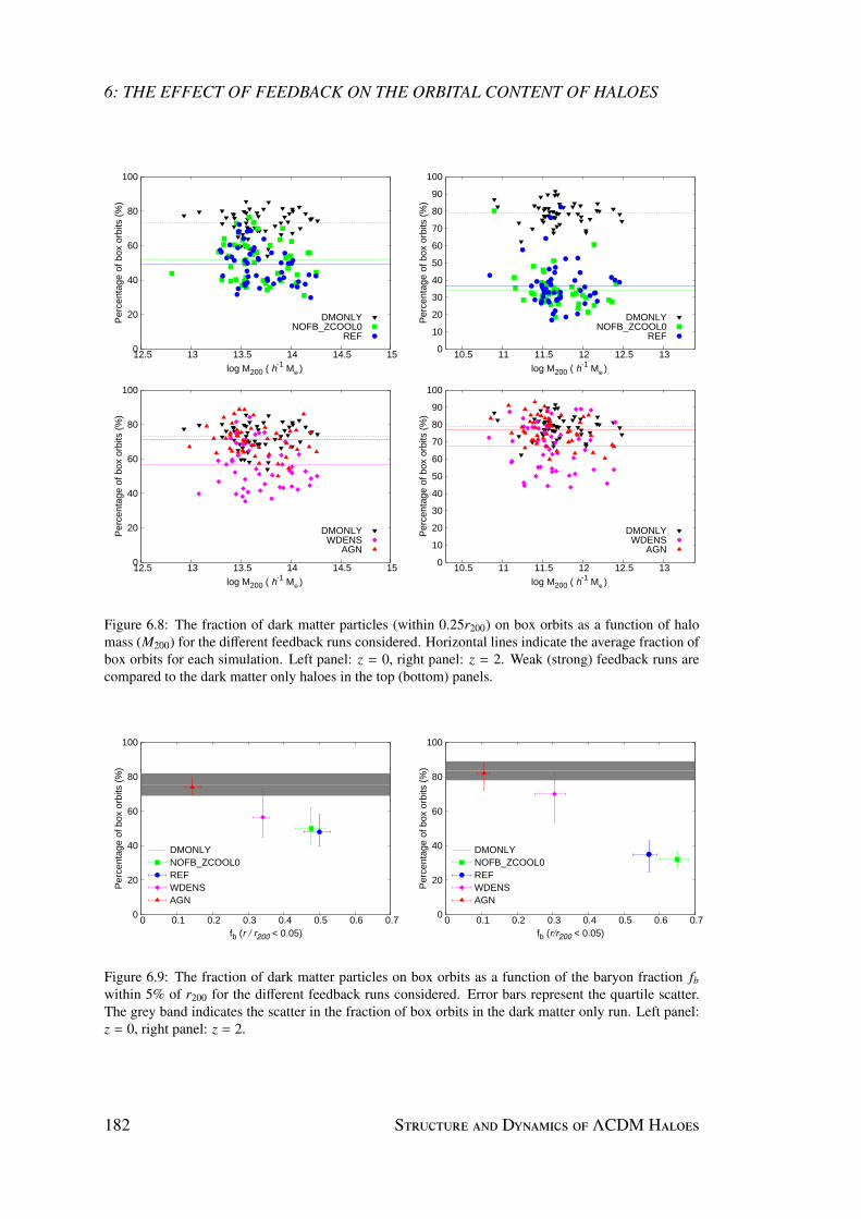
6: THE EFFECT OF FEEDBACK ON THE ORBITAL CONTENT OF HALOES
0
20
40
60
80
100
12.5 13 13.5 14 14.5 15
Per
cent
age
of b
ox o
rbits
(%
)
log M200 ( h-1 MO• )
DMONLYNOFB_ZCOOL0
REF 0
10
20
30
40
50
60
70
80
90
100
10.5 11 11.5 12 12.5 13
Per
cent
age
of b
ox o
rbits
(%
)
log M200 ( h-1 MO• )
DMONLYNOFB_ZCOOL0
REF
0
20
40
60
80
100
12.5 13 13.5 14 14.5 15
Per
cent
age
of b
ox o
rbits
(%
)
log M200 ( h-1 MO• )
DMONLYWDENS
AGN 0
10
20
30
40
50
60
70
80
90
100
10.5 11 11.5 12 12.5 13
Per
cent
age
of b
ox o
rbits
(%
)
log M200 ( h-1 MO• )
DMONLYWDENS
AGN
Figure 6.8: The fraction of dark matter particles (within 0.25r200) on box orbits as a function of halomass (M200) for the different feedback runs considered. Horizontal lines indicate the average fraction ofbox orbits for each simulation. Left panel: z = 0, right panel: z = 2. Weak (strong) feedback runs arecompared to the dark matter only haloes in the top (bottom) panels.
0
20
40
60
80
100
0 0.1 0.2 0.3 0.4 0.5 0.6 0.7
Per
cent
age
of b
ox o
rbits
(%
)
fb (r / r200 < 0.05)
DMONLYNOFB_ZCOOL0REFWDENSAGN
0
20
40
60
80
100
0 0.1 0.2 0.3 0.4 0.5 0.6 0.7
Per
cent
age
of b
ox o
rbits
(%
)
fb (r/r200 < 0.05)
DMONLYNOFB_ZCOOL0REFWDENSAGN
Figure 6.9: The fraction of dark matter particles on box orbits as a function of the baryon fraction fbwithin 5% of r200 for the different feedback runs considered. Error bars represent the quartile scatter.The grey band indicates the scatter in the fraction of box orbits in the dark matter only run. Left panel:z = 0, right panel: z = 2.
182 S D ΛCDM H
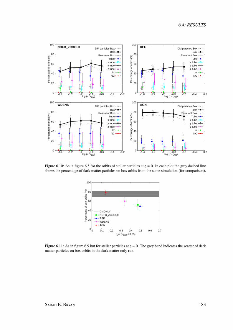
6.4: RESULTS
0
20
40
60
80
100
-1.4 -1.2 -1 -0.8 -0.6 -0.4 -0.2
Per
cent
age
of o
rbits
(%
)
log (r / r200)
NOFB_ZCOOL0 DM particles BoxBox
Resonant BoxTube
x tubey tubez tube
IrrNC
0
20
40
60
80
100
-1.4 -1.2 -1 -0.8 -0.6 -0.4 -0.2
Per
cent
age
of o
rbits
(%
)
log (r / r200)
REF DM particles BoxBox
Resonant BoxTube
x tubey tubez tube
IrrNC
0
20
40
60
80
100
-1.4 -1.2 -1 -0.8 -0.6 -0.4 -0.2
Per
cent
age
of o
rbits
(%
)
log (r / r200)
WDENS DM particles BoxBox
Resonant BoxTube
x tubey tubez tube
IrrNC
0
20
40
60
80
100
-1.4 -1.2 -1 -0.8 -0.6 -0.4 -0.2
Per
cent
age
of o
rbits
(%
)
log (r / r200)
AGN DM particles BoxBox
Resonant BoxTube
x tubey tubez tube
IrrNC
Figure 6.10: As in figure 6.5 for the orbits of stellar particles at z = 0. In each plot the grey dashed lineshows the percentage of dark matter particles on box orbits from the same simulation (for comparison).
0
20
40
60
80
100
0 0.1 0.2 0.3 0.4 0.5 0.6 0.7
Per
cent
age
of b
ox o
rbits
(%
)
fb (r / r200 < 0.05)
DMONLYNOFB_ZCOOL0REFWDENSAGN
Figure 6.11: As in figure 6.9 but for stellar particles at z = 0. The grey band indicates the scatter of darkmatter particles on box orbits in the dark matter only run.
S E. B 183
6: THE EFFECT OF FEEDBACK ON THE ORBITAL CONTENT OF HALOES
6.4.2 Orbits of Stellar Particles
In Figure 6.10 the orbital classifications of stellar particles at z = 0 are shown. As in
figure 6.5 the different feedback implementations are compared. In each plot the grey
dashed line shows the percentage of dark matter particles on box orbits from the same
simulations (for comparison). As in figure 6.9 the dependence of the fraction of stellar
particle box orbits (within 0.05r200) on the central baryon fraction fb is shown in figure
6.11.
The orbital content described by the stellar particles is remarkably similar to that
drawn from the orbits of dark matter particles. While the dark matter and stellar par-
ticles are selected from the same radius, one might expect a different trend due to the
formation history of the stellar particles. Since the potential and initial conditions are
drawn from the main S halo, distinct subhaloes and satellites are not included
and the stellar population considered here is associated with the central galaxy and
the diffuse intra-halo component. A full analysis of the history of the stellar particles
(such as when they were stripped from parent subhaloes) could prove insightful. The
results presented here seem to indicate that either they were stripped a long time ago
and have forgotten their dynamical history or subhaloes bringing in the stars are not
biased significantly with respect to the main distribution - the velocity bias (measured
as the ratio of galaxy to dark matter velocity dispersion) is weak (e.g. Springel et al.
2001a).
6.4.3 Orbits of Subhaloes
The orbits of the subhaloes associated with each S main halo have also been
considered. The initial position was taken to be an average over the ten most bound
particles and velocity of the subhalo is assumed to be that of the most bound parti-
cle. The orbits of the 20 most massive subhaloes within rvir of each of the 50 haloes
discussed above are explored. The subhaloes trace a region much further out than dis-
cussed previously (mean r/rvir = 0.6 compared to a mean value of r/rvir = 0.12 for the
184 S D ΛCDM H

6.4: RESULTS
dark matter and stellar particles). Subhaloes are also subject to tidal stripping.
The fraction of subhaloes on box orbits as a function of the halo mass M200 is
shown in figure 6.12. All of the runs indicate a similar fraction of box orbits. The
region probed by the subhaloes is less strongly affected by the presence of baryons
than the central regions discussed before.
Figure 6.13 emphasises this point, showing the median fraction and scatter of sub-
haloes on box orbits as a function of the central baryon fraction at z = 0. Comparing
this plot to figures 6.9 and 6.11 shows that a similar fraction of subhaloes and dark
matter (or stellar) particles are on box orbits in the weak or no feedback runs. The
main difference observed in this plot is the drop in the fraction of box orbits in the
dark matter and AGN runs expected at large radii. The fraction of box orbits is ex-
pected to decrease with radius (as observed in the strong feedback and dark matter
only cases), but baryons act to flatten the slope in the central regions, giving rise to an
almost constant box orbit fraction with radii.
This behaviour is already visible in figure 6.5, where the difference between the
fraction of box orbits in dissipational and dissipationless simulations decreases with
radius.
The drop in the fraction of dark matter subhaloes on box orbits may also be due
to the tidal disruption of the subhaloes as they pass close to the centre of the halo.
Cooling would act to increase the central concentration of both the subhalo and the
main halo. Strong feedback, such as the AGN run, would be more efficient in the main
halo than in the subhalo and it is likely that tidal disruption would be less severe for
these runs than in the dark matter only case.
S E. B 185

6: THE EFFECT OF FEEDBACK ON THE ORBITAL CONTENT OF HALOES
0
20
40
60
80
100
12.5 13 13.5 14 14.5 15
Per
cent
age
of b
ox o
rbits
(%
)
log M200 ( h-1 MO• )
DMONLYNOFB_ZCOOL0REF
0
20
40
60
80
100
12.5 13 13.5 14 14.5 15P
erce
ntag
e of
box
orb
its (
%)
log M200 ( h-1 MO• )
DMONLYWDENSAGN
Figure 6.12: The fraction of subhaloes on box orbits as a function of the halo mass M200 for the differentsimulations considered. The left (right) panel compares orbits of subhaloes from the dark matter onlysimulation to runs with weak (strong) feedback.
0
20
40
60
80
100
0 0.1 0.2 0.3 0.4 0.5 0.6 0.7
Per
cent
age
of b
ox o
rbits
(%
)
fb (r / r200 < 0.05)
DMONLYNOFB_ZCOOL0REFWDENSAGN
Figure 6.13: As in figure 6.9 but for subhaloes z = 0. The grey band indicates the scatter of dark mattersubhaloes on box orbits in the dark matter only run.
186 S D ΛCDM H

6.5: NUMERICAL ISSUES
6.5 Numerical Issues
In this section the convergence radius rconv and resolution effects are considered in
order to show that the results presented in this chapter are well converged. The choices
of halo definition and basis sets are also discussed.
6.5.1 Convergence Radius
Power et al. (2003) showed that numerical convergence in inner regions of dark matter
haloes was achieved outside of the convergence radius rconv. This radius is defined to
ensure that the two-body dynamical relaxation time within this radius is comparable to
the age of the Universe (trelax & t0). Power et al. (2003) define
trelax (r)tcirc (r200)
=N (r)
8 ln N (r)r/Vc
r200/V200=
√2008
N (r)ln N (r)
(ρ
ρcrit
)−1/2
, (6.9)
where tcirc (r200) ∼ t0 and N(r) is the number of particles enclosed within radius r.
Power et al. (2003) show that the density profile converges at radii that enclose a suffi-
cient number of particles to ensure that trelax(r) ≥ 0.6t0.
The convergence radius depends on halo size and the resolution of the simulation
and sets a minimum resolved length scale or the analysis. Figure 6.14 shows an esti-
mate of the convergence radius as a fraction of M200 for the haloes used in this analysis.
From this plot one can see that the innermost radial bin considered in this chapter is
beyond the convergence radius (i.e. rconv < rmin).
6.5.2 Resolution Effects
In order to quantify the effects of resolution on the orbital content, the 5123 particle
run from the DMONLY simulations (with a softening length of 2 h−1 kpc) is compared
with the corresponding lower resolution runs (containing 2563 and 1283 particles and
with softening lengths of 4 and 8 h−1 kpc, respectively). In Figure 6.15 the fraction of
box orbits found in the 1283 simulation is shown in blue, the 2563 simulation in green
S E. B 187

6: THE EFFECT OF FEEDBACK ON THE ORBITAL CONTENT OF HALOES
0.01
0.015
0.02
0.025
0.03
0.035
0.04
0.045
12.8 13 13.2 13.4 13.6 13.8 14 14.2
r conv/r200
log M200 ( h-1 MO• )
DMONLY
0
0.005
0.01
0.015
0.02
0.025
0.03
0.035
0.04
0.045
10.8 11 11.2 11.4 11.6 11.8 12 12.2 12.4 12.6
r conv/r200
log M200 ( h-1 MO• )
DMONLY
Figure 6.14: Convergence radius rconv for the dark matter only simulation at z = 0 (left) and z = 2 (right).The horizontal line shows the innermost bin considered in this analysis. Orbits of particles beyond theconvergence radius are studied.
0
20
40
60
80
100
-1.4 -1.2 -1 -0.8 -0.6 -0.4 -0.2
Per
cent
age
of b
ox o
rbits
(%
)
log(r/r200)
DMONLY N512N256N128
0
20
40
60
80
100
-1.4 -1.2 -1 -0.8 -0.6 -0.4 -0.2
Per
cent
age
of b
ox o
rbits
(%
)
log(r/r200)
REF N512N256N128
Figure 6.15: The effect of resolution on z = 0 results. Results from the 1283 simulation are shown inblue, the 2563 simulation in green and the 5123 simulation used for this analysis in red. The fraction ofbox orbits found in the dark matter only run is shown in the left plot. The fraction of box orbits foundin the weak feedback run (REF) is shown in the right plot. The convergence radius for each simulationis shown as a vertical line.
and the 5123 simulation used for this analysis in red. The fraction of box orbits found
in the dark matter only run is shown in the left plot while the fraction of box orbits
found in the weak feedback run (REF) is shown on the right. Only relaxed haloes that
are matched between the different resolution runs are considered.
188 S D ΛCDM H

6.5: NUMERICAL ISSUES
0
20
40
60
80
100
-1.4 -1.2 -1 -0.8 -0.6 -0.4 -0.2
Per
cent
age
of b
ox o
rbits
(%
)
log(r/r200)
DMONLY SOSUBFOF
0
20
40
60
80
100
-1.4 -1.2 -1 -0.8 -0.6 -0.4 -0.2
Per
cent
age
of b
ox o
rbits
(%
)
log(r/r200)
REF SOSUBFOF
Figure 6.16: The effect of halo definition on the orbital content of haloes, using the 5123 particle simu-lations at z = 0. The left plot shows the fraction of box orbits in the dark matter only simulations, whilethe right plot shows the fraction of box orbits in the weak feedback run (REF). Results obtained if haloesare defined using the algorithm are shown in blue, those using the main S halo are shown ingreen and those obtained using SO are shown in red. The orbital content of a halo is not particularlysensitive to the halo definition.
6.5.3 Effect of Halo Definition
To explore the effect of the halo definition on the results presented here, the three com-
mon definitions of a group – , main subhalo as identified by S and the SO
approach – were used. The orbital content of the haloes is not significantly affected
by the halo definition, as shown in Figure 6.16. The main subhalo is therefore used
throughout this analysis, this has the advantage of providing a smooth potential, unper-
turbed by substructure. The radial dependence of the orbital content is scaled by the
spherical overdensity definition of r200. In the dark matter only simulations the frac-
tion of box orbits does not depend on the choice of groupfinder. In the weak feedback
run (REF) the S haloes show a slightly lower fraction of box orbits, however
the trends discussed in this chapter are not significantly affected by the choice of the
groupfinder.
6.5.4 Choice of Basis Set and Expansion Coefficients
The basis set used in this analysis is constructed so that the lowest order terms represent
the Hernquist profile (Hernquist 1990). Twelve radial terms and six angular terms
S E. B 189

6: THE EFFECT OF FEEDBACK ON THE ORBITAL CONTENT OF HALOES
Table 6.2: Classifications of orbits from the most massive relaxed cluster at z = 0. Different numbersof expansion coefficients have been used to reconstruct the potential using the Hernquist basis set (top)and the Clutton-Brock basis set (bottom).
(n,l) Box Tube Irr resonant box x-tube z-tube Not classified20,6 0.510 0.386 0.014 0.194 0.056 0.326 0.09020,4 0.528 0.376 0.006 0.194 0.034 0.340 0.09012,6 0.582 0.314 0.016 0.188 0.044 0.268 0.08812,4 0.532 0.370 0.009 0.162 0.042 0.328 0.0888,6 0.564 0.318 0.024 0.188 0.054 0.258 0.0098,4 0.484 0.400 0.006 0.144 0.030 0.366 0.110
20,6 0.582 0.337 0.008 0.238 0.038 0.298 0.08020,4 0.490 0.424 0.008 0.178 0.032 0.392 0.07812,6 0.458 0.428 0.012 0.182 0.029 0.398 0.10212,4 0.430 0.476 0.008 0.144 0.034 0.438 0.0868,6 0.422 0.468 0.008 0.186 0.014 0.452 0.1028,4 0.412 0.456 0.022 0.176 0.010 0.440 0.110
are used as this has been found to be sufficient to reproduce the potential to within a
few percent of the N-body potential. Table 6.2 shows the orbital content of the most
massive relaxed cluster from the weak feedback simulation at z = 0 as determined
using both the Hernquist and the Clutton-Brock basis sets. This cluster has a mass of
2 × 10¹⁴ h−1 M. The orbital content does not vary significantly when more terms are
used. Varying the number of expansion coefficients affects the orbital classifications on
the percent level. The choice of basis set is not found to affect the reconstruction of the
potential significantly. Figure 6.17 shows the difference in potential computed using
SCF method and the potential computed using the Direct Summation method. Blue
points indicates the SCF potential has been computed using the Hernquist basis set,
while green points show the SCF potential computed using the Clutton-Brock basis
set.
6.6 Summary and Discussion
The orbital content of a large sample of haloes extracted from state-of-the-art high-
resolution cosmological hydrodynamical simulations has been explored in order to
190 S D ΛCDM H

6.6: SUMMARY AND DISCUSSION
-0.006
-0.004
-0.002
0
0.002
0.004
0.006
0.008
0.01
0.012
500 1000 1500 2000
(SC
F -
Nbo
dy P
oten
tial)/
Nbo
dy P
oten
tial
r (kpc/h)
REF -- Hernquist-Ostriker,n=12, l=6REF -- Clutton-Brock, n=12, l=6
Figure 6.17: Difference in potential as computed by the SCF method and the Direct-Summation ap-proach for the most massive weak feedback (REF) halo. For the blue points the SCF has been computedusing the basis set of Hernquist-Ostriker, while for green points the SCF potential is calculated usingthe Clutton-Brock basis set.
study what observational signatures may result. Dark matter only haloes are dominated
by box orbits out to 0.25r200. This is not surprising as box orbits are known to be
required to support the triaxial haloes characteristic of dark matter only haloes. The
fraction of box orbits is found to decrease with increasing distance from the halo centre;
this is mirrored by an increase in the fraction of tube orbits. Roughly half of the
box orbits are found to exhibit resonance. The fraction of resonant box orbits is also
found to decrease with radius. Very few of the orbits analysed in the dark matter only
simulations were found to be on y-tubes and a negligible fraction of the orbits where
classified as irregular. The tube orbits are dominated by x-tubes in the central region,
and the fraction of both x- and z-tube orbits is found to increase with increasing radius;
z-tubes dominate the fraction of tube orbits at larger radii.
The orbital content of these dark matter haloes does not appear to be strongly de-
pendent on basic halo properties such as spin, mass, redshift and dynamical state in
either the dark matter only or the weak feedback runs for the range of parameters con-
sidered here.
By comparing simulations run with no feedback, with stellar feedback and with
feedback from AGN, the fraction of box orbits in the central region is found to decrease
S E. B 191

6: THE EFFECT OF FEEDBACK ON THE ORBITAL CONTENT OF HALOES
when baryonic physics is included. Baryons are able to cool and condense to the centre
of the halo, and this central concentration tends to transform box orbits into tube orbits.
Increasing the strength of the feedback implementation is found to reduce the central
concentration of baryons, and increase the fraction of box orbits. The orbital content
described by the stellar particles is found to be remarkably similar to that drawn from
the orbits of dark matter particles. Subhaloes probe a more extended region of the halo
and are subject to tidal stripping. The different implementations of the baryon physics
do not appear to change the fraction of subhaloes on box orbits significantly. Typically
∼ 50% of the subhaloes are found to be on box orbits.
192 S D ΛCDM H

7
Summary and Future Work
Currently, with simulations such as the Millennium Simulation (Springel et al. 2005b),
Aquarius (Springel et al. 2008), Via Lactea (Diemand et al. 2008) and Ghalo (Stadel
et al. 2009), we have a good understanding of dark matter structure formation. Dark
matter haloes formed in a ΛCDM cosmology appear to share many universal proper-
ties, such as their internal morphology (see, for example, Navarro et al. 1996; Navarro
et al. 1997; Bullock et al. 2001; Duffy et al. 2008) and an abundance of substructure
(Klypin et al. 1999; Moore et al. 1999; Gao et al. 2004a,b; Diemand et al. 2007b) and
are typically thought to be triaxial (Frenk et al. 1988; Dubinski and Carlberg 1991;
Warren et al. 1992; Cole and Lacey 1996; Jing and Suto 2002; Bailin and Steinmetz
2005b; Allgood et al. 2006; Maccio et al. 2006; Bett et al. 2007). These generic pre-
dictions are a result of hierarchical structure formation and the dissipationless nature
of dark matter. The role of baryons on structure formation is much more uncertain and
has become the focus of galaxy formation studies. A thorough understanding of the
role of baryons in galaxy formation and evolution is essential, not only because most
observations are only able to trace baryonic matter but also because of the complex
role it may play in the evolution of the dark matter halo itself.
The merging process will leave imprints on the structure and dynamics of the rem-
nant galaxy. Studying these relic imprints will provide information about the galaxies’
formation history. However, the complex interplay between mergers and dissipational
S E. B 193
7: SUMMARY AND FUTURE WORK
effects needs to be considered. In order to fully optimise the use of such observational
signatures, comparisons with simulations such as these are essential. In this thesis
state-of-the-art simulations have been used to explore three such observational signa-
tures: the abundance of substructure, the shape of haloes and the orbital content of the
haloes.
This work incorporates two different approaches to baryonic and gas physics in
the simulations. The first uses simple semi-analytic prescriptions to approximate the
complicated physical processes involved in galaxy formation (see section 3.7) and the
second implements SPH techniques (see section 3.4.1). These simulations provide a
unique opportunity to analyse the effects of baryons and implemented feedback tech-
niques on a large sample of haloes evolved within a cosmological setting.
A generic prediction of CDM models is an abundance of substructure. While this
matches well with observations on cluster scales, galactic scales have proven a more
stringent test on galaxy formation models. Simulations on galaxy scales predict al-
most an order of magnitude more satellites than are actually observed in the Milky
Way. These results are however reconcilable as fainter and fainter objects are being
detected observationally and the suppression of star formation in the smallest objects
is modelled. Gravitational lensing is a unique probe of the mass along the line of sight
in that it is not sensitive to the type of matter (baryonic or otherwise), but only to the
total mass. CDM substructure has been proposed as an explanation of the anomalous
flux ratios seen in gravitational lens systems. While there is sufficient mass in simu-
lated substructures, its not clear that substructures are able to survive in the very central
regions probed by lensing. Surprisingly, about 50% of lenses in the Cosmic Lens All-
Sky Survey (CLASS) appear to have luminous satellites within ∼ 5 h−1 kpc of the main
lensing galaxies.
In chapter 4 the Millennium Simulation (Springel et al. 2005b), combined with
galaxy catalogues from semi-analytical models (De Lucia and Blaizot 2007), is used
to study the predicted frequency of such satellites in simulated haloes. The fraction of
haloes that host bright satellites within the (projected) central regions is similar for red
194 S D ΛCDM H

and blue hosts and is found to increase as a function of host halo mass and redshift.
However, even in group-sized haloes at z = 1, the predicted number of haloes found
to host a luminous satellite galaxy is lower than that observed in CLASS. It is worth
noting that most of the satellites found in the inner regions are ‘orphan’ galaxies where
the dark matter haloes have been completely stripped. Thus the agreement crucially
depends on the true survival rate of these ‘orphan’ galaxies. While the limited number
of lenses in CLASS makes it difficult to draw any strong conclusions, the predicted
number of haloes found to host a luminous satellite galaxy is significantly lower than
that observed in CLASS.
This work was extended to include companions of all elliptical galaxies, in or-
der to compare the fractions of satellites in field and lens galaxies (see Jackson et al.
2010). The frequencies of luminous satellites in the central regions of galaxies selected
from SDSS, COSMOS and SLACS were studied, significantly increasing the sample
size. No significant difference was found between the populations of field and lens
systems. The fractions of systems found to host a luminous companion within the pro-
jected central region in the SDSS, COSMOS and SLACS samples are even lower than
that observed in the semi-analytic galaxy catalogue and considerably lower than the
CLASS lenses. The frequency of luminous satellites in CLASS appears to be anoma-
lously high, however firm conclusions await the acquisition of a large sample of high
redshift lenses.
In chapter 5, the predicted distributions of the spin and shape of dark matter haloes
are investigated and the roles of baryons and the physical prescriptions of stellar and
black hole feedback are examined. The spin distribution of haloes extracted from
the baryon runs is not significantly different to that of dark matter only haloes when
computed over the whole halo. However, in the central regions where baryons are
expected to dominate, haloes from weak feedback simulations tend to have higher
median spin values than haloes from high feedback runs. The spin distribution in the
central region of strong feedback simulations is comparable to the distribution found
for dark matter only haloes. Dark matter only haloes typically have triaxial to prolate
S E. B 195

7: SUMMARY AND FUTURE WORK
shapes and their radial shape profiles are close to flat. More massive haloes are found
to be less spherical and more prolate than lower mass haloes. Baryons act to make the
haloes more spherical and weak stellar feedback runs are able to produce almost oblate
haloes, while stellar and AGN feedback runs result in prolate haloes similar to those
found in dark matter only simulations. Baryons are also shown to have a significant
effect on the shape of the dark matter distribution. The shapes of the simulated haloes
are shown to be in agreement with a wide range of observational estimates of the shapes
of elliptical galaxies.
In chapter 6, the orbital content of simulated haloes is analysed, with particular
focus on the role of energy ejected (feedback) from SNe and black holes in shaping the
orbital content of haloes. How the orbital content of these haloes depends on several
key parameters (such as their mass, redshift and dynamical state) is also considered.
Efficient cooling causes the haloes to become centrally concentrated and this results
in a decrease in the fraction of orbits passing close to the centre. As the feedback
efficiency from stars and black holes increases, the central concentration is reduced
and the number of orbits passing close to the centre increases. The Gaia satellite, to be
launched in 2012, will provide a kinematic census of our Galaxy. To optimise the use
of this data, comparison with simulations will be crucial.
What is clear from this work is that baryons play an important role in the formation
and evolution of galaxies and an understanding of these processes is incomplete with-
out careful consideration of gas physics. Studying the central regions of haloes may
place strong constraints on formation theories. While studying this region is made
complicated by the effects of baryons and limited resolution (both observationally and
in simulations) it may yield some of the most useful constraints on galaxy formation
models by providing insight into the important physical processes that govern galaxy
evolution. Galaxies found in the innermost regions of a halo are likely to be signifi-
cantly affected by physical processes such as tidal stripping and, in simulations, are the
most sensitive to numerical effects. Comparison between observations and simulations
in this regime is essential. Fortunately, rapid advances in computational power and in-
196 S D ΛCDM H

creasingly sophisticated treatment of gas physics is now allowing us to probe this in
more detail than ever before.
Proposed Future Directions
The orbital content of dark matter haloes in the Phoenix simulations (Liang Gao1) will
be analysed using the techniques described in chapter 6. The Phoenix simulations are
high-resolution dark matter simulations and consist of 9 clusters simulated at differ-
ent resolutions, the highest resolution run containing 109 particles within the virial
radius. The unprecedented resolution of the Phoenix cluster simulations will make it
possible to probe the dynamics of substructure to a unparallelled level, allowing for
the study of orbits of subhaloes covering an exceptionally large range in mass. This
resolution would be ideal for exploring dynamic mass segregation (massive subhaloes
are more centrally concentrated than their lower mass counterparts) in detail. This
would provide valuable information about the origin of the mass segregation and the
relative importance of the mechanisms present in clusters that drive the evolution of
the subhaloes and their associated galaxies.
The force resolution of the simulations would allow us to probe the very central
regions of the cluster. Semi-analytic catalogues run on these simulations will allow
for a study of the dynamics of satellite galaxies covering a wide range of masses,
luminosities, colours, star formation histories and accretion times. The orbital content
of the simulated clusters and their subhalo and satellite populations will be assessed.
As haloes are known to rotate (Bailin and Steinmetz 2004; Bryan and Cress 2007),
it would also be interesting to investigate the effects of a live halo, considering the
time evolution of the potential, on the dynamics of the system. This can be achieved
by tracing the halo through time using merger trees. The halo potential can be esti-
mated using the SCF method at the redshifts recorded in the simulation and the SCF
coefficients can be interpolated between these time intervals.
1private communication
S E. B 197

7: SUMMARY AND FUTURE WORK
Further applications of this work would be to use the predicted orbits to explore disc
heating, angular momentum transfer from satellites and the tidal stripping of satellites
in high-resolution simulations such as Phoenix, Aquarius and OWLS. Discs are able to
provide strong constraints on the merging history of a system and angular momentum
transfer from satellites to the dark matter may play an important role in shaping the
density profile of a system.
198 S D ΛCDM H

References
Aarseth, S. J. Dynamical evolution of clusters of galaxies, I. MNRAS, 126:223, 1963.
Adelman-McCarthy, J. K., Agueros, M. A., Allam, S. S. et al. The sixth data release
of the Sloan Digital Sky Survey. ApJS, 175:297, 2008.
Allgood, B., Flores, R. A., Primack, J. R. et al. The shape of dark matter haloes:
Dependence on mass, redshift, radius and formation. MNRAS, 367:1781, 2006.
Amendt, P. and Cuddeford, P. Pseudomoment stellar dynamics. 1: Spheroidal galactic
equilibria. ApJ, 435:93, 1994.
Arnaboldi, M., Capaccioli, M., Cappellaro, E. et al. Studies of narrow polar rings
around E Galaxies. I - Observations and model of AM 2020-504. A&A, 267:21,1993.
Bailin, J. and Steinmetz, M. Figure rotation of cosmological dark matter halos. ApJ,616:27, 2004.
Bailin, J. and Steinmetz, M. Can satellite dwarfs excite galactic warps? In H. Jerjen& B. Binggeli, editor, IAU Colloq. 198: Near-fields cosmology with dwarf elliptical
galaxies, 207–210. 2005a.
Bailin, J. and Steinmetz, M. Internal and external alignment of the shapes and angular
momenta of ΛCDM halos. ApJ, 627:647, 2005b.
Banerjee, A. and Jog, C. J. The flattened dark matter halo of M31 as deduced from the
observed H I scale heights. ApJ, 685:254, 2008.
Bardeen, J. M., Bond, J. R., Kaiser, N. et al. The statistics of peaks of Gaussian random
fields. ApJ, 304:15, 1986.
Barkana, R. and Loeb, A. Detecting reionization in the star formation histories of
high-redshift galaxies. MNRAS, 371:395, 2006.
Barnes, J. and Hut, P. A hierarchical O(N log N) force-calculation algorithm. Nature,
S E. B 199

REFERENCES
324:446, 1986.
Barnes, J. E. Transformations of galaxies. I - Mergers of equal-mass stellar disks. ApJ,393:484, 1992.
Barnes, J. E. and Hernquist, L. Transformations of galaxies. II. Gasdynamics in merg-
ing disk galaxies. ApJ, 471:115, 1996a.
Barnes, J. E. and Hernquist, L. Transformations of galaxies. II. Gasdynamics in merg-
ing disk galaxies. ApJ, 471:115, 1996b.
Baugh, C. M. A primer on hierarchical galaxy formation: the semi-analytical ap-
proach. Reports of Progress in Physics, 69:3101, 2006.
Baumgardt, H. and Makino, J. Dynamical evolution of star clusters in tidal fields.MNRAS, 340:227, 2003.
Becquaert, J. and Combes, F. The 3D geometry of dark matter halos. A&A, 325:41,1997.
Belokurov, V., Zucker, D. B., Evans, N. W. et al. Cats and dogs, hair and a hero: A
quintet of new Milky Way companions. ApJ, 654:897, 2007.
Bett, P., Eke, V., Frenk, C. S. et al. The spin and shape of dark matter haloes in the
Millennium simulation of a Λ cold dark matter universe. MNRAS, 376:215, 2007.
Bienayme, O., Soubiran, C., Mishenina, T. V. et al. Vertical distribution of galactic
disk stars. A&A, 446:933, 2006.
Binney, J., May, A. and Ostriker, J. P. On the flattening of dark haloes. MNRAS,226:149, 1987.
Binney, J. and Spergel, D. Spectral stellar dynamics. ApJ, 252:308, 1982.
Binney, J. and Tremaine, S. Galactic dynamics. Princeton, NJ, Princeton UniversityPress, 1987, 747 p., 1987.
Blanton, M. R., Hogg, D. W., Bahcall, N. A. et al. The galaxy luminosity function and
luminosity density at redshift z = 0.1. ApJ, 592:819, 2003.
Bode, P., Ostriker, J. P. and Turok, N. Halo formation in warm dark matter models.ApJ, 556:93, 2001.
Bolton, A. S., Burles, S., Koopmans, L. V. E. et al. The Sloan lens ACS survey. I. A
large spectroscopically selected sample of massive early-type lens galaxies. ApJ,638:703, 2006.
Bolton, A. S., Burles, S., Koopmans, L. V. E. et al. The Sloan lens ACS survey. V. The
200 S D ΛCDM H

REFERENCES
full ACS strong-lens sample. ApJ, 682:964, 2008.
Bond, J. R., Cole, S., Efstathiou, G. et al. Excursion set mass functions for hierarchical
Gaussian fluctuations. ApJ, 379:440, 1991.
Bonnor, W. B. Jeans’ formula for gravitational instability. MNRAS, 117:104, 1957.
Booth, C. M. and Schaye, J. Cosmological simulations of the growth of supermassive
black holes and feedback from active galactic nuclei: Method and tests. MNRAS,398:53, 2009.
Bower, R. G., Benson, A. J., Malbon, R. et al. Breaking the hierarchy of galaxy
formation. MNRAS, 370:645, 2006.
Brown, M. L., Ade, P., Bock, J. et al. Improved measurements of the temperature and
polarization of the cosmic microwave background from QUaD. ApJ, 705:978, 2009.
Browne, I. W. A., Wilkinson, P. N., Jackson, N. J. F. et al. The Cosmic Lens All-Sky
Survey - II. Gravitational lens candidate selection and follow-up. MNRAS, 341:13,2003.
Bryan, G. L. and Norman, M. L. Statistical properties of x-ray clusters: Analytic and
numerical comparisons. ApJ, 495:80, 1998.
Bryan, S. E. and Cress, C. M. Figure rotation of dark haloes in cold dark matter
simulations. MNRAS, 380:657, 2007.
Bullock, J. S. Shapes of dark matter halos. In P. Natarajan, editor, The Shapes of
Galaxies and their Dark Matter Haloes, 1099. 2002.
Bullock, J. S., Dekel, A., Kolatt, T. S. et al. A universal angular momentum profile for
galactic halos. ApJ, 555:240, 2001.
Buote, D. A. and Canizares, C. R. X-ray constraints on the intrinsic shape of the
lenticular galaxy NGC 1332. ApJ, 457:177, 1996.
Buote, D. A. and Canizares, C. R. The nature of the X-ray emission and the mass
distributions in two early-type galaxies. ApJ, 474:650, 1997.
Buote, D. A. and Canizares, C. R. The shapes and sizes of elliptical galaxy halos
from x-ray observations. In D. Zaritsky, editor, Galactic Halos, volume 136 ofAstronomical Society of the Pacific Conference Series, 289. 1998.
Capak, P., Aussel, H., Ajiki, M. et al. The first release COSMOS optical and near-IR
data and Catalog. ApJS, 172:99, 2007.
Carpintero, D. D. and Aguilar, L. A. Orbit classification in arbitrary 2D and 3D
S E. B 201

REFERENCES
potentials. MNRAS, 298:1, 1998.
Carroll, S. M., Press, W. H. and Turner, E. L. The cosmological constant. ARA&A,30:499, 1992.
Chabrier, G. Galactic stellar and substellar initial mass function. PASP, 115:763,2003.
Chandrasekhar, S. and Henrich, L. R. An attempt to interpret the relative abundances
of the elements and their isotopes. ApJ, 95:288, 1942.
Chen, J., Rozo, E., Dalal, N. et al. Astrometric perturbations in substructure lensing.ApJ, 659:52, 2007.
Clowe, D., Bradac, M., Gonzalez, A. H. et al. A direct empirical proof of the existence
of dark matter. ApJL, 648:L109, 2006.
Clutton-Brock, M. The gravitational field of three dimensional galaxies. Astrophysicsand Space Science, 23:55, 1973.
Cohn, J. D. and Kochanek, C. S. The effects of massive substructures on image multi-
plicities in gravitational lenses. ApJ, 608:25, 2004.
Cole, S. Modeling galaxy formation in evolving dark matter halos. ApJ, 367:45, 1991.
Cole, S. and Lacey, C. The structure of dark matter haloes in hierarchical clustering
models. MNRAS, 281:716, 1996.
Contopoulos, G. A third integral of motion in a galaxy. ZAp, 49:273, 1960.
Couchman, H. M. P. and Rees, M. J. Pregalactic evolution in cosmologies with cold
dark Matter. MNRAS, 221:53, 1986.
Croton, D. J., Springel, V., White, S. D. M. et al. The many lives of active galac-
tic nuclei: cooling flows, black holes and the luminosities and colours of galaxies.MNRAS, 365:11, 2006.
Dalal, N. and Kochanek, C. S. Direct detection of cold dark matter substructure. ApJ,572:25, 2002.
Dalla Vecchia, C. and Schaye, J. Simulating galactic outflows with kinetic supernova
feedback. MNRAS, 387:1431, 2008.
Davis, M., Efstathiou, G., Frenk, C. S. et al. The evolution of large-scale structure in
a universe dominated by cold dark matter. ApJ, 292:371, 1985.
de Lorenzi, F., Debattista, V. P., Gerhard, O. et al. NMAGIC: A fast parallel im-
plementation of a χ2-made-to-measure algorithm for modelling observational data.
202 S D ΛCDM H

REFERENCES
MNRAS, 376:71, 2007.
De Lucia, G. and Blaizot, J. The hierarchical formation of the brightest cluster galax-
ies. MNRAS, 375:2, 2007.
De Lucia, G., Kauffmann, G. and White, S. D. M. Chemical enrichment of the intr-
acluster and intergalactic medium in a hierarchical galaxy formation model. MN-RAS, 349:1101, 2004.
De Lucia, G., Springel, V., White, S. D. M. et al. The formation history of elliptical
galaxies. MNRAS, 366:499, 2006.
de Zeeuw, T. and Franx, M. Kinematics of gas in a triaxial Galaxy. ApJ, 343:617,1989.
de Zeeuw, T. and Franx, M. Structure and dynamics of elliptical galaxies. ARA&A,29:239, 1991.
Debattista, V. P., Moore, B., Quinn, T. et al. The causes of halo shape changes induced
by cooling baryons: Disks versus substructures. ApJ, 681:1076, 2008.
Debattista, V. P. and Sellwood, J. A. Warped galaxies from misaligned angular mo-
menta. ApJL, 513:L107, 1999.
Dehnen, W. Tailoring triaxial N-body models via a novel made-to-measure method.MNRAS, 395:1079, 2009.
Diemand, J., Kuhlen, M. and Madau, P. Dark matter substructure and gamma-ray
annihilation in the Milky Way halo. ApJ, 657:262, 2007a.
Diemand, J., Kuhlen, M. and Madau, P. Formation and evolution of galaxy dark matter
halos and their substructure. ApJ, 667:859, 2007b.
Diemand, J., Kuhlen, M., Madau, P. et al. Clumps and streams in the local dark matter
distribution. Nature, 454:735, 2008.
Dolag, K., Borgani, S., Murante, G. et al. Substructures in hydrodynamical cluster
simulations. MNRAS, 399:497, 2009.
Doroshkevich, A. G., Zel’Dovich, Y. B. and Novikov, I. D. The origin of galaxies in
an expanding universe. Soviet Astronomy, 11:233, 1967.
Dubinski, J. The effect of dissipation on the shapes of dark halos. ApJ, 431:617, 1994.
Dubinski, J. and Carlberg, R. G. The structure of cold dark matter halos. ApJ, 378:496,1991.
Duffy, A. R., Schaye, J., Kay, S. T. et al. Dark matter halo concentrations in the Wilkin-
S E. B 203
REFERENCES
son Microwave Anisotropy Probe year 5 Cosmology. MNRAS, 390:L64, 2008.
Duffy, A. R., Schaye, J., Kay, S. T. et al. Impact of baryon physics on dark matter
structures: A detailed simulation study of halo density profiles. MNRAS, 405:2161,2010.
Earman, J. Lambda: The constant that refuses to die. Archive for History of ExactSciences, 55:189, 2001. 10.1007/s004070000025.
Efstathiou, G. Suppressing the formation of dwarf galaxies via photoionization. MN-RAS, 256:43P, 1992.
Efstathiou, G., Davis, M., White, S. D. M. et al. Numerical techniques for large
cosmological N − body simulations. ApJS, 57:241, 1985.
Efstathiou, G. and Eastwood, J. W. On the clustering of particles in an expanding
universe. MNRAS, 194:503, 1981.
Eisenstein, D. J. Dark energy and cosmic sound [review article]. New AstronomyReviews, 49:360, 2005.
Eisenstein, D. J. and Hu, W. Power spectra for cold dark matter and its variants. ApJ,511:5, 1999.
Eke, V. R., Cole, S. and Frenk, C. S. Cluster evolution as a diagnostic for Omega.MNRAS, 282:263, 1996.
Evrard, A. E., Summers, F. J. and Davis, M. Two-fluid simulations of galaxy formation.ApJ, 422:11, 1994.
Ewald, P. P. Die Berechnung optischer und elektrostatischer Gitterpotentiale. Annalender Physik, 369:253, 1921.
Faber, S. M. and Jackson, R. E. Velocity dispersions and mass-to-light ratios for
elliptical galaxies. ApJ, 204:668, 1976.
Faltenbacher, A. and White, S. D. M. Assembly bias and the dynamical structure of
dark matter halos. ApJ, 708:469, 2010.
Fasano, G., Amico, P., Bertola, F. et al. The intrinsic shapes of galactic discs. MNRAS,262:109, 1993.
Fassnacht, C. D. and Cohen, J. G. Keck spectroscopy of three gravitational lens systems
discovered in the JVAS and CLASS surveys. AJ, 115:377, 1998.
Fassnacht, C. D., Gal, R. R., Lubin, L. M. et al. Mass along the line of sight to
the gravitational lens B1608+656: Galaxy groups and implications for H0. ApJ,
204 S D ΛCDM H

REFERENCES
642:30, 2006.
Fellhauer, M., Belokurov, V., Evans, N. W. et al. The origin of the bifurcation in the
Sagittarius stream. ApJ, 651:167, 2006.
Ferland, G. J., Korista, K. T., Verner, D. A. et al. CLOUDY 90: Numerical simulation
of plasmas and their spectra. PASP, 110:761, 1998.
Franx, M. and de Zeeuw, T. Elongated disks and the scatter in the Tully-Fisher rela-
tion. ApJL, 392:L47, 1992.
Franx, M., Illingworth, G. and de Zeeuw, T. The ordered nature of elliptical galaxies
- Implications for their intrinsic angular momenta and shapes. ApJ, 383:112, 1991.
Franx, M., van Gorkom, J. H. and de Zeeuw, T. Evidence for axisymmetric halos: The
case of IC 2006. ApJ, 436:642, 1994.
Frenk, C. S., White, S. D. M., Davis, M. et al. The formation of dark halos in a universe
dominated by cold dark matter. ApJ, 327:507, 1988.
Gamow, G. Expanding universe and the origin of elements. Physical Review, 70:572,1946.
Gao, L., De Lucia, G., White, S. D. M. et al. Galaxies and subhaloes in ΛCDM galaxy
clusters. MNRAS, 352:L1, 2004a.
Gao, L., White, S. D. M., Jenkins, A. et al. The subhalo populations of ΛCDM dark
haloes. MNRAS, 355:819, 2004b.
Garnavich, P. M., Jha, S., Challis, P. et al. Supernova limits on the cosmic equation of
state. ApJ, 509:74, 1998.
Gerhard, O. E. and Binney, J. Triaxial galaxies containing massive black holes or
central density cusps. MNRAS, 216:467, 1985.
Ghigna, S., Moore, B., Governato, F. et al. Density profiles and substructure of dark
matter halos: Converging results at ultra-high numerical resolution. ApJ, 544:616,2000.
Gingold, R. A. and Monaghan, J. J. Smoothed particle hydrodynamics - Theory and
application to non-spherical stars. MNRAS, 181:375, 1977.
Gnedin, N. Y. Effect of reionization on structure formation in the universe. ApJ,542:535, 2000.
Gnedin, O. Y., Gould, A., Miralda-Escude, J. et al. Probing the shape of the galactic
halo with hypervelocity stars. ApJ, 634:344, 2005.
S E. B 205

REFERENCES
Granato, G. L., De Zotti, G., Silva, L. et al. A physical model for the coevolution of
QSOs and their spheroidal hosts. ApJ, 600:580, 2004.
Guo, Q., White, S., Boylan-Kolchin, M. et al. From dwarf spheroidals to cDs: Simu-
lating the galaxy population in a LCDM cosmology. ArXiv e-prints, 2010.
Guth, A. H. Inflationary universe: A possible solution to the horizon and flatness
problems. Phys. Rev. D, 23:347, 1981.
Haardt, F. and Madau, P. Modelling the UV/X-ray cosmic background with CUBA. InD. M. Neumann & J. T. V. Tran, editor, Clusters of Galaxies and the High Redshift
Universe Observed in X-rays. 2001.
Helmi, A. Is the dark halo of our galaxy spherical? MNRAS, 351:643, 2004.
Hennawi, J. F., Dalal, N., Bode, P. et al. Characterizing the cluster lens population.ApJ, 654:714, 2007.
Henriques, B., Bertone, S. and Thomas, P. Disruption of dwarf galaxies in semi-
analytic models. arXiv:astro-ph/0706.3814, 2007.
Hernquist, L. An analytical model for spherical galaxies and bulges. ApJ, 356:359,1990.
Hernquist, L., Hut, P. and Makino, J. Discreteness noise versus force errors in N−Body
simulations. ApJL, 402:L85, 1993.
Hernquist, L. and Katz, N. TREESPH - A unification of SPH with the hierarchical tree
method. ApJS, 70:419, 1989.
Hernquist, L. and Ostriker, J. P. A self-consistent field method for galactic dynamics.ApJ, 386:375, 1992.
Hockney, R. W. and Eastwood, J. W. Computer simulation using particles. 1981.
Hoekstra, H., Yee, H. K. C. and Gladders, M. D. Properties of galaxy dark matter
halos from weak lensing. ApJ, 606:67, 2004.
Hoffman, L., Cox, T. J., Dutta, S. et al. Orbital structure of merger remnants: Trends
with gas fraction in 1:1 mergers. ArXiv e-prints, 2010.
Hofner, P. and Sparke, L. S. Time evolution of galactic WARPS. ApJ, 428:466, 1994.
Holmberg, E. On the clustering tendencies among the nebulae. II. A study of encoun-
ters between laboratory models of stellar systems by a new integration procedure.
ApJ, 94:385, 1941.
Holmberg, E. A study of physical groups of galaxies. Arkiv for Astronomi, 5:305,
206 S D ΛCDM H
REFERENCES
1969.
Hopkins, P. F., Bahcall, N. A. and Bode, P. Cluster alignments and ellipticities in
ΛCDM cosmology. ApJ, 618:1, 2005.
Hubble, E. A relation between distance and radial velocity among extra-galactic neb-
ulae. Proceedings of the National Academy of Science, 15:168, 1929.
Ibata, R., Lewis, G. F., Irwin, M. et al. Great circle tidal streams: Evidence for a
nearly spherical massive dark halo around the Milky Way. ApJ, 551:294, 2001.
Jackson, N., Bryan, S. E., Mao, S. et al. Satellites in the field and lens galaxies:
SDSS/COSMOS versus SLACS/CLASS. MNRAS, 403:826, 2010.
Jeans, J. H. Astronomy and Cosmogony. 1928.
Jenkins, A. Second-order Lagrangian perturbation theory initial conditions for resim-
ulations. MNRAS, 403:1859, 2010.
Jenkins, A., Frenk, C. S., White, S. D. M. et al. The mass function of dark matter
haloes. MNRAS, 321:372, 2001.
Jesseit, R., Naab, T. and Burkert, A. Orbital structure of collisionless merger remnants:
On the origin of photometric and kinematic properties of elliptical and S0 galaxies.MNRAS, 360:1185, 2005.
Jing, Y. P. and Suto, Y. Triaxial modeling of halo density profiles with high-resolution
N − body simulations. ApJ, 574:538, 2002.
Johnston, K. V., Law, D. R. and Majewski, S. R. A two micron all sky survey view of
the Sagittarius dwarf galaxy. III. Constraints on the flattening of the galactic halo.ApJ, 619:800, 2005.
Katz, N. and Gunn, J. E. Dissipational galaxy formation. I - Effects of Gasdynamics.ApJ, 377:365, 1991.
Kauffmann, G., Colberg, J. M., Diaferio, A. et al. Clustering of galaxies in a hierar-
chical universe - I. Methods and results at z=0. MNRAS, 303:188, 1999.
Kauffmann, G., White, S. D. M. and Guiderdoni, B. The formation and evolution of
galaxies within merging dark matter haloes. MNRAS, 264:201, 1993.
Kazantzidis, S., Kravtsov, A. V., Zentner, A. R. et al. The effect of gas cooling on the
shapes of dark matter halos. ApJL, 611:L73, 2004.
Keeton, C. R. and Moustakas, L. A. A new channel for detecting dark matter substruc-
ture in galaxies: gravitational lens time delays. arXiv:astro-ph/0805.0309, 2008.
S E. B 207

REFERENCES
Kennicutt, R. C., Jr. The global Schmidt law in star-forming galaxies. ApJ, 498:541,1998.
Kimm, T. and Yi, S. K. Intrinsic axis ratio distribution of early-type galaxies from the
Sloan Digital Sky Survey. ApJ, 670:1048, 2007.
Klypin, A., Kravtsov, A. V., Valenzuela, O. et al. Where are the missing galactic
satellites? ApJ, 522:82, 1999.
Knebe, A., Gill, S. P. D., Gibson, B. K. et al. Anisotropy in the distribution of satellite
Galaxy orbits. ApJ, 603:7, 2004.
Kochanek, C., Falco, E., C. Impey, J. L. et al. http://www.cfa.harvard.edu/castles/.2008.
Kochanek, C. S. The implications of lenses for galaxy structure. ApJ, 373:354, 1991.
Kochanek, C. S. Evidence for dark matter in MG 1654+134. ApJ, 445:559, 1995.
Kolb, E. and Turner, M. The early universe. Addison-Wesley Publishing Company,1993.
Komatsu, E., Dunkley, J., Nolta, M. R. et al. Five-Year Wilkinson Microwave
Anisotropy Probe observations: Cosmological interpretation. ApJS, 180:330, 2009.
Komatsu, E., Smith, K. M., Dunkley, J. et al. Seven-year Wilkinson Microwave
Anisotropy Probe (WMAP) Observations: Cosmological Interpretation. ApJS,192:18, 2011.
Koopmans, L. V. E., de Bruyn, A. G. and Jackson, N. The edge-on spiral gravitational
lens B1600+434. MNRAS, 295:534, 1998.
Koopmans, L. V. E., de Bruyn, A. G., Marlow, D. R. et al. A new radio double lens
from CLASS: B1127+385. MNRAS, 303:727, 1999.
Koopmans, L. V. E., Treu, T., Fassnacht, C. D. et al. The Hubble constant from the
gravitational lens B1608+656. ApJ, 599:70, 2003.
Kowalski, M., Rubin, D., Aldering, G. et al. Improved cosmological constraints from
new, old, and combined supernova data sets. ApJ, 686:749, 2008.
Kravtsov, A. V., Gnedin, O. Y. and Klypin, A. A. The tumultuous lives of galactic
dwarfs and the missing satellites problem. ApJ, 609:482, 2004.
Kuijken, K. and Tremaine, S. On the ellipticity of the galactic disk. ApJ, 421:178,1994.
Lacey, C. and Cole, S. Merger rates in hierarchical models of galaxy formation. MN-
208 S D ΛCDM H
REFERENCES
RAS, 262:627, 1993a.
Lacey, C. and Cole, S. Merger rates in hierarchical models of galaxy formation. MN-RAS, 262:627, 1993b.
Lacey, C. and Cole, S. Merger rates in hierarchical models of galaxy formation - Part
Two - Comparison with N − body simulations. MNRAS, 271:676, 1994.
Lacey, C. and Silk, J. Tidally triggered galaxy formation. I - Evolution of the galaxy
luminosity function. ApJ, 381:14, 1991.
Lambas, D. G., Maddox, S. J. and Loveday, J. On the true shapes of galaxies. MNRAS,258:404, 1992.
Larson, D., Dunkley, J., Hinshaw, G. et al. Seven-Year Wilkinson Microwave
Anisotropy Probe (WMAP) Observations: Power spectra and WMAP-derived pa-
rameters. ArXiv e-prints, 2010.
Law, D. R. and Majewski, S. R. Assessing the Milky Way satellites associated with the
Sagittarius dwarf spheroidal galaxy. ApJ, 718:1128, 2010.
Law, D. R., Majewski, S. R. and Johnston, K. V. Evidence for a triaxial Milky Way
dark matter halo from the Sagittarius stellar tidal stream. ApJL, 703:L67, 2009.
Lemaıtre, G. Un Univers homogene de masse constante et de rayon croissant rendant
compte de la vitesse radiale des nebuleuses extra-galactiques. Annales de la SocieteScietifique de Bruxelles, 47:49, 1927.
Lewis, A., Challinor, A. and Lasenby, A. Efficient computation of cosmic microwave
background anisotropies in closed Friedmann-Robertson-Walker models. ApJ,538:473, 2000.
Liddle, A. An Introduction to Modern Cosmology, Second Edition. 2003.
Lindblad, B. Die Milchstraße. Handbuch der Astrophysik, 5:937, 1933.
Long, R. J. and Mao, S. Made-to-measure Galaxy models - I. Methodology. MNRAS,405:301, 2010.
Lucy, L. B. A numerical approach to the testing of the fission hypothesis. AJ, 82:1013,1977.
Maccio, A. V., Dutton, A. A. and van den Bosch, F. C. Concentration, spin and shape
of dark matter haloes as a function of the cosmological model: WMAP1, WMAP3
and WMAP5 results. MNRAS, 391:1940, 2008.
Maccio, A. V., Moore, B., Stadel, J. et al. Radial distribution and strong lensing
S E. B 209

REFERENCES
statistics of satellite galaxies and substructure using high-resolution ΛCDM hydro-
dynamical simulations. MNRAS, 366:1529, 2006.
Madau, P., Diemand, J. and Kuhlen, M. Dark matter subhalos and the dwarf satellites
of the Milky Way. arXiv:astro-ph/0802.2265, 2008.
Makino, J., Taiji, M., Ebisuzaki, T. et al. GRAPE-4: A massively parallel special-
purpose computer for collisional N-Body simulations. ApJ, 480:432, 1997.
Mandelbaum, R., Hirata, C. M., Broderick, T. et al. Ellipticity of dark matter haloes
with galaxy-galaxy weak lensing. MNRAS, 370:1008, 2006.
Mandelbaum, R., McDonald, P., Seljak, U. et al. Precision cosmology from the Lyman
α forest: power spectrum and bispectrum. MNRAS, 344:776, 2003.
Mao, S. and Schneider, P. Evidence for substructure in lens galaxies? MNRAS,295:587, 1998.
Martınez-Delgado, D., Penarrubia, J., Juric, M. et al. The Virgo stellar overdensity:
Mapping the infall of the Sagittarius tidal stream onto the Milky Way disk. ApJ,660:1264, 2007.
McKean, J. P., Browne, I. W. A., Jackson, N. J. et al. CLASS B2108+213: A new
wide-separation gravitational lens system. MNRAS, 356:1009, 2005.
McKean, J. P., Koopmans, L. V. E., Browne, I. W. A. et al. Keck spectroscopy of
Cosmic Lens All-Sky Survey gravitational lenses. MNRAS, 350:167, 2004.
McKean, J. P., Koopmans, L. V. E., Flack, C. E. et al. High-resolution imaging of
the anomalous flux ratio gravitational lens system CLASS B2045+265: Dark or
luminous satellites? MNRAS, 378:109, 2007.
Merrifield, M. R. The galactic halo and CDM. In S. Ryder, D. Pisano, M. Walker, &K. Freeman, editor, Dark Matter in Galaxies, volume 220 of IAU Symposium, 431.2004.
Merritt, D. and Valluri, M. Resonant orbits in triaxial galaxies. AJ, 118:1177, 1999.
Meszaros, P. The behaviour of point masses in an expanding cosmological substratum.A&A, 37:225, 1974.
Metcalf, R. B. The importance of intergalactic structure to gravitationally lensed
quasars. ApJ, 629:673, 2005.
Monaghan, J. J. Smoothed particle hydrodynamics. ARA&A, 30:543, 1992.
Monaghan, J. J. and Lattanzio, J. C. A refined particle method for astrophysical prob-
210 S D ΛCDM H
REFERENCES
lems. A&A, 149:135, 1985.
Moore, B., Ghigna, S., Governato, F. et al. Dark matter substructure within galactic
halos. ApJL, 524:L19, 1999.
Moore, B., Katz, N. and Lake, G. On the destruction and overmerging of dark halos
in dissipationless N − Body simulations. ApJ, 457:455, 1996.
Myers, S. T., Jackson, N. J., Browne, I. W. A. et al. The Cosmic Lens All-Sky Survey -
I. Source selection and observations. MNRAS, 341:1, 2003.
Nakamura, K. and Group, P. D. Review of particle physics. Journal of Physics G:Nuclear and Particle Physics, 37(7A):075021, 2010.
Navarro, J. F. and Benz, W. Dynamics of cooling gas in galactic dark halos. ApJ,380:320, 1991.
Navarro, J. F., Frenk, C. S. and White, S. D. M. The assembly of galaxies in a hierar-
chically clustering universe. MNRAS, 275:56, 1995.
Navarro, J. F., Frenk, C. S. and White, S. D. M. The structure of cold dark matter
halos. ApJ, 462:563, 1996.
Navarro, J. F., Frenk, C. S. and White, S. D. M. A universal density profile from
hierarchical clustering. ApJ, 490:493, 1997.
Neto, A. F., Gao, L., Bett, P. et al. The statistics of Λ CDM halo concentrations.MNRAS, 381:1450, 2007.
New, K. C. B., Tohline, J. E., Frank, J. et al. A physical model of warped galaxy disks.ApJ, 503:632, 1998.
O’Brien, J. C., Freeman, K. C. and van der Kruit, P. C. The dark matter halo shape of
edge-on disk galaxies. IV. UGC 7321. A&A, 515:A63, 2010.
Oguri, M. The Mass Distribution of SDSS J1004+4112 Revisited. PASJ, 62:1017,2010.
Oguri, M., Lee, J. and Suto, Y. Arc statistics in triaxial dark matter halos: Testing the
collisionless cold dark matter paradigm. ApJ, 599:7, 2003.
Oh, S., Brook, C., Governato, F. et al. The central slope of dark matter cores in dwarf
galaxies: Simulations vs. THINGS. ArXiv e-prints, 2010.
Olive, K. A., Steigman, G. and Walker, T. P. Primordial nucleosynthesis : Theory and
observations. Phys. Rep., 333:389, 2000.
Olling, R. P. The highly flattened dark matter halo of NGC 4244. AJ, 112:481, 1996.
S E. B 211

REFERENCES
Olling, R. P. and Merrifield, M. R. Two measures of the shape of the dark halo of the
Milky Way. MNRAS, 311:361, 2000.
Ostriker, E. C. and Binney, J. J. Warped and tilted galactic discs. MNRAS, 237:785,1989.
Parkinson, H., Cole, S. and Helly, J. Generating dark matter halo merger trees. MN-RAS, 383:557, 2008.
Peacock, J. A., Cole, S., Norberg, P. et al. A measurement of the cosmological mass
density from clustering in the 2dF galaxy redshift survey. Nature, 410:169, 2001.
Peebles, P. J. E. Origin of the angular momentum of galaxies. ApJ, 155:393, 1969.
Peebles, P. J. E. The large-scale structure of the Universe. 1980.
Peebles, P. J. E. Principles of physical cosmology. 1993.
Penzias, A. A. and Wilson, R. W. A measurement of excess antenna temperature at
4080 Mc/s. ApJ, 142:419, 1965.
Percival, W. J., Sutherland, W., Peacock, J. A. et al. Parameter constraints for flat
cosmologies from cosmic microwave background and 2dFGRS power spectra. MN-RAS, 337:1068, 2002.
Perlmutter, S., Aldering, G., Goldhaber, G. et al. Measurements of omega and lambda
from 42 High-Redshift supernovae. ApJ, 517:565, 1999.
Pfenniger, D., Combes, F. and Martinet, L. Is dark matter in spiral galaxies cold gas?
I. Observational constraints and dynamical clues about galaxy evolution. A&A,285:79, 1994.
Piontek, F. and Steinmetz, M. The modelling of feedback processes in cosmological
simulations of disc galaxy formation. MNRAS, 1632, 2010.
Poggianti, B. M. K and evolutionary corrections from UV to IR. A&AS, 122:399,1997.
Power, C., Navarro, J. F., Jenkins, A. et al. The inner structure of ΛCDM haloes - I. A
numerical convergence study. MNRAS, 338:14, 2003.
Press, W. H. and Schechter, P. Formation of galaxies and clusters of galaxies by self-
similar gravitational condensation. ApJ, 187:425, 1974.
Rahmati, A. and Jalali, M. A. New biorthogonal potential-density basis functions.MNRAS, 393:1459, 2009.
Rees, M. J. Lyman absorption lines in quasar spectra - Evidence for gravitationally-
212 S D ΛCDM H

REFERENCES
confined gas in dark minihaloes. MNRAS, 218:25P, 1986.
Rees, M. J. and Ostriker, J. P. Cooling, dynamics and fragmentation of massive gas
clouds - Clues to the masses and radii of galaxies and clusters. MNRAS, 179:541,1977.
Reichardt, C. L., Ade, P. A. R., Bock, J. J. et al. High-resolution CMB power spectrum
from the complete ACBAR data set. ApJ, 694:1200, 2009.
Riess, A. G., Filippenko, A. V., Challis, P. et al. Observational evidence from su-
pernovae for an accelerating universe and a cosmological constant. AJ, 116:1009,1998.
Riess, A. G., Press, W. H. and Kirshner, R. P. A precise distance indicator: Type IA
supernova multicolor light-curve shapes. ApJ, 473:88, 1996.
Rix, H. and Zaritsky, D. Nonaxisymmetric structures in the stellar disks of galaxies.ApJ, 447:82, 1995.
Rusin, D., Kochanek, C. S., Norbury, M. et al. B1359+154: A Six-Image lens produced
by a z ˜= 1 compact group of galaxies. ApJ, 557:594, 2001.
Rusin, D., Norbury, M., Biggs, A. D. et al. High-resolution observations and mass
modelling of the CLASS gravitational lens B1152+199. MNRAS, 330:205, 2002.
Ryden, B. The intrinsic shapes of elliptical galaxies. ApJ, 396:445, 1992.
Sackett, P. D. The shape of dark matter halos. In D. R. Merritt, M. Valluri, & J. A. Sell-wood, editor, Galaxy Dynamics - A Rutgers Symposium, volume 182 of Astronomi-
cal Society of the Pacific Conference Series, 393. 1999.
Sackett, P. D., Rix, H., Jarvis, B. J. et al. The flattened dark halo of polar-ring galaxy
NGC 4650A: A conspiracy of shapes? ApJ, 436:629, 1994.
Sales, L. V., Navarro, J. F., Lambas, D. G. et al. Satellite galaxies and fossil groups in
the Millennium simulation. MNRAS, 382:1901, 2007.
Schaye, J. Star formation thresholds and galaxy edges: Why and where. ApJ, 609:667,2004.
Schaye, J. and Dalla Vecchia, C. On the relation between the Schmidt and Kennicutt-
Schmidt star formation laws and its implications for numerical simulations. MN-RAS, 383:1210, 2008.
Schaye, J., Dalla Vecchia, C., Booth, C. M. et al. The physics driving the cosmic star
formation history. MNRAS, 402:1536, 2010.
S E. B 213
REFERENCES
Schechter, P. L. and Moore, C. B. The lensing Galaxy in MG 0414 + 0534. AJ, 105:1,1993.
Schneider, P., Kochanek, C. S. and Wambsganss, J. Gravitational lensing: Strong,
weak and micro. 2006.
Schwarzschild, M. A numerical model for a triaxial stellar system in dynamical equi-
librium. ApJ, 232:236, 1979.
Sciama, D. W. On the role of a strongly flattened galactic halo in the decaying dark
matter hypothesis. MNRAS, 244:1P, 1990.
Scoville, N., Abraham, R. G., Aussel, H. et al. COSMOS: Hubble space telescope
observations. ApJS, 172:38, 2007.
Seljak, U. and Zaldarriaga, M. A line-of-sight integration approach to cosmic mi-
crowave background anisotropies. ApJ, 469:437, 1996.
Sheth, R. K. and Tormen, G. On the environmental dependence of halo formation.MNRAS, 350:1385, 2004.
Shin, E. M. and Evans, N. W. The effect of satellite galaxies on gravitational lensing
flux ratios. MNRAS, 385:2107, 2008.
Silk, J. On the fragmentation of cosmic gas clouds. I - The formation of galaxies and
the first generation of stars. ApJ, 211:638, 1977.
Smoot, G. F., Bennett, C. L., Kogut, A. et al. Structure in the COBE differential
microwave radiometer first-year maps. ApJL, 396:L1, 1992.
Spergel, D. N., Bean, R., Dore, O. et al. Three-year Wilkinson Microwave Anisotropy
Probe (WMAP) observations: Implications for cosmology. ApJS, 170:377, 2007.
Spergel, D. N., Verde, L., Peiris, H. V. et al. First-year Wilkinson Microwave
Anisotropy Probe (WMAP) observations: determination of cosmological parame-
ters. ApJS, 148:175, 2003.
Springel, V. The cosmological simulation code GADGET-2. MNRAS, 364:1105, 2005.
Springel, V., Di Matteo, T. and Hernquist, L. Modelling feedback from stars and black
holes in galaxy mergers. MNRAS, 361:776, 2005a.
Springel, V. and Hernquist, L. Cosmological smoothed particle hydrodynamics simu-
lations: the entropy equation. MNRAS, 333:649, 2002.
Springel, V. and Hernquist, L. Cosmological smoothed particle hydrodynamics simu-
lations: a hybrid multiphase model for star formation. MNRAS, 339:289, 2003.
214 S D ΛCDM H

REFERENCES
Springel, V., Wang, J., Vogelsberger, M. et al. The Aquarius Project: the subhaloes of
galactic haloes. MNRAS, 391:1685, 2008.
Springel, V., White, S. D. M. and Hernquist, L. The shapes of simulated dark matter
halos. In S. Ryder, D. Pisano, M. Walker, & K. Freeman, editor, Dark Matter in
Galaxies, volume 220 of IAU Symposium, 421. 2004.
Springel, V., White, S. D. M., Jenkins, A. et al. Simulations of the formation, evolution
and clustering of galaxies and quasars. Nature, 435:629, 2005b.
Springel, V., White, S. D. M., Tormen, G. et al. Populating a cluster of galaxies - I.
Results at z=0. MNRAS, 328:726, 2001a.
Springel, V., Yoshida, N. and White, S. D. M. GADGET: A code for collisionless and
gasdynamical cosmological simulations. New Astronomy, 6:79, 2001b.
Stadel, J., Potter, D., Moore, B. et al. Quantifying the heart of darkness with GHALO
- a multibillion particle simulation of a galactic halo. MNRAS, 398:L21, 2009.
Statler, T. S. Self-consistent models of perfect triaxial galaxies. ApJ, 321:113, 1987.
Steiman-Cameron, T. Y., Kormendy, J. and Durisen, R. H. The remarkable twisted
disk of NGC 4753 and the shapes of galactic halos. AJ, 104:1339, 1992.
Stoehr, F., White, S. D. M., Springel, V. et al. Dark matter annihilation in the halo of
the Milky Way. MNRAS, 345:1313, 2003.
Sugimoto, D., Chikada, Y., Makino, J. et al. A special-purpose computer for gravita-
tional many-body problems. Nature, 345:33, 1990.
Syer, D. and Tremaine, S. Made-to-measure N − body systems. MNRAS, 282:223,1996.
Tegmark, M., Strauss, M. A., Blanton, M. R. et al. Cosmological parameters from
SDSS and WMAP. Phys. Rev. D, 69(10):103501, 2004.
Thoul, A. A. and Weinberg, D. H. Hydrodynamic simulations of galaxy formation. II.
Photoionization and the formation of low-mass galaxies. ApJ, 465:608, 1996.
Tinker, J., Kravtsov, A. V., Klypin, A. et al. Toward a halo mass function for precision
cosmology: The limits of universality. ApJ, 688:709, 2008.
Tissera, P. B. and Dominguez-Tenreiro, R. Dark matter halo structure in CDM hydro-
dynamical simulations. MNRAS, 297:177, 1998.
Toomre, A. Mergers and some consequences. In B. M. Tinsley & R. B. Larson, editor,Evolution of galaxies and stellar populations, 401. 1977.
S E. B 215

REFERENCES
Treu, T., Gavazzi, R., Gorecki, A. et al. The SLACS Survey. VIII. The relation between
environment and internal structure of early-type galaxies. ApJ, 690:670, 2009.
Turner, E. L., Ostriker, J. P. and Gott, J. R., III. The statistics of gravitational lenses -
The distributions of image angular separations and lens redshifts. ApJ, 284:1, 1984.
Valluri, M., Debattista, V. P., Quinn, T. et al. The orbital evolution induced by baryonic
condensation in triaxial haloes. MNRAS, 129, 2010.
van der Marel, R. P. Flattening and kinematics of the galactic halo. MNRAS, 248:515,1991.
Van Waerbeke, L., Mellier, Y., Pello, R. et al. Likelihood analysis of cosmic shear on
simulated and VIRMOS-DESCART data. A&A, 393:369, 2002.
von Hoerner, S. Die numerische integration des n-Korper-Problems fur Sternhaufen,
II. ZAp, 57:47, 1963.
Wang, J., De Lucia, G., Kitzbichler, M. G. et al. The dependence of galaxy formation
on cosmological parameters: Can we distinguish between the WMAP1 and WMAP3
parameter sets? MNRAS, 384:1301, 2008.
Wang, L., Li, C., Kauffmann, G. et al. Modelling galaxy clustering in a high-resolution
simulation of structure formation. MNRAS, 371:537, 2006.
Warren, M. S., Quinn, P. J., Salmon, J. K. et al. Dark halos formed via dissipationless
collapse. I - Shapes and alignment of angular momentum. ApJ, 399:405, 1992.
Weinberg, S. Gravitation and Cosmology: Principles and applications of the general
theory of relativity. 1972.
White, S. D. M. Simulations of merging galaxies. MNRAS, 184:185, 1978.
White, S. D. M. Formation and evolution of galaxies. In R. Schaeffer, J. Silk, M. Spiro,& J. Zinn-Justin, editor, Cosmology and large scale Structure, 349. 1996.
White, S. D. M. and Frenk, C. S. Galaxy formation through hierarchical clustering.ApJ, 379:52, 1991.
White, S. D. M., Navarro, J. F., Evrard, A. E. et al. The baryon content of galaxy
clusters - a challenge to cosmological orthodoxy. Nature, 366:429, 1993.
White, S. D. M. and Rees, M. J. Core condensation in heavy halos - A two-stage theory
for galaxy formation and clustering. MNRAS, 183:341, 1978.
Whitmore, B. C., McElroy, D. B. and Schweizer, F. The shape of the dark halo in
polar-ring galaxies. ApJ, 314:439, 1987.
216 S D ΛCDM H
REFERENCES
Wiersma, R. P. C., Schaye, J. and Smith, B. D. The effect of photoionization on the
cooling rates of enriched, astrophysical plasmas. MNRAS, 393:99, 2009.
Yadav, J., Bharadwaj, S., Pandey, B. et al. Testing homogeneity on large scales in the
Sloan Digital Sky Survey Data release one. MNRAS, 364:601, 2005.
York, T., Jackson, N., Browne, I. W. A. et al. CLASS B0631+519: Last of the cosmic
lens all-sky survey lenses. MNRAS, 361:259, 2005.
Zel’dovich, Y. B. Gravitational instability: An approximate theory for large density
perturbations. A&A, 5:84, 1970.
Zwicky, F. On the masses of nebulae and of clusters of nebulae. ApJ, 86:217, 1937.
S E. B 217
REFERENCES
‘Begin at the beginning,’ the King said, very gravely,
‘and go on till you come to the end:
then stop.’
- Lewis Carroll.
218 S D ΛCDM H