structure and vibrational spectroscopy of salt water/air...

Structure and Vibrational Spectroscopy of Salt

Water/Air Interfaces: Predictions from Classical

Molecular Dynamics Simulations

Eric C. Brown,1 Martin Mucha,2 Pavel Jungwirth2 and Douglas J. Tobias1*

1Department of Chemistry, and

Environmental Molecular Sciences Institute,

University of California, Irvine

Irvine, California 92697-2025, USA

and

2Institute of Organic Chemistry and Biochemistry, and

Center for Complex Molecular Systems and Biomolecules,

Academy of Sciences of the Czech Republic

Flemingovo nam. 2, 16610 Prague 6, Czech Republic

∗To whom correpondence should be addressed: [email protected]

1

Abstract

We report the Sum Frequency Generation (SFG) spectra of aqueous sodium iodide

interfaces computed with the methodology outlined by Morita and Hynes (J. Phys.

Chem. B 2002, 106, 673), which is based on molecular dynamics simulations. The

calculated spectra are in qualitative agreement with experiment. Our simulations

show that the addition of sodium iodide to water leads to an increase in SFG intensity

in the region of 3400 cm−1, which corresponds to an increase in ordering of hydrogen-

bonded water molecules. Depth-resolved orientational distribution functions suggest

that the ion double layer orders water molecules which are about one water layer

below the Gibbs dividing surface. We attribute the increase in SFG intensity to

these ordered subsurface water molecules which are present in the aqueous sodium

iodide/air interfaces, but are absent in the neat water/air interface.

1

1 Introduction

Aqueous aerosols and other particulate matter play an important role in the various chemi-

cal reactions which occur in the atmosphere. In the marine boundary layer aqueous sea-salt

aerosols are ubiquitous. [1] The bursting of air bubbles trapped by wave action produces

fine aerosols that are comprised primarily of alkali and alkaline earth halide salts dissolved

in water. These salt water aerosols serve as a source of reactant and as a substrate for

various heterogeneous reactions with polluting gases.

An example is the production of molecular chlorine via the oxidation of chloride by

hydroxyl radical. In an aerosol chamber, Knipping et al. monitored the appearance of

chlorine and the disappearance of ozone (from which hydroxyl radical was generated by

photolysis in the presence of water vapor), and sought to deduce the reaction mechanism(s)

by fitting their kinetic data to a sizable battery of known bulk aqueous phase chemical

reactions and their respective rates. [2] This particular modeling attempt based on bulk

phase chemistry failed to predict the observed production of molecular chlorine under the

conditions of the experiment.

Molecular dynamics (MD) simulations predicted that heavier halides may exist at in-

terfaces in surprisingly high abundance. [3, 4, 5, 6] The results of the MD simulations

suggested that the interface can be rich in reactant chloride, and it is essential to take

this into account when proposing a kinetic model that could match experimental data.

[2] Indeed, when the aforementioned experimental results were analyzed using an interfa-

cial mechanism that took into account the fact that ions could be present at interfaces,

2

the kinetics data were well-reproduced. [2] Hydroxide anions, predicted to be a product

of the interfacial reaction, were subsequently detected in NaCl aerosol particles following

exposure to hydroxyl radical. [7]

The results of the MD simulations are supported by the fact that experimental and

theoretical studies on small clusters (e.g., (H2O)6Cl−) reveal that the halide ions are not

completely solvated by water molecules, but instead exist in configurations where a large

portion of the halide ion is exposed. [8] In contrast, similar studies on small clusters with

alkali cations (e.g. (H2O)6Na+) reveal that the cations are almost totally encapsulated by

coordinating water molecules. [9]

The notion that atomic ions exist at the interface in surfactant-like excess is seemingly

inconsistent with a straightforward application of the Gibbs adsorption relation. If, in

accord with experiment and surface electrolyte theory, the surface tension of a salt solution

increases relative to that of pure water, then the concentration of solute (in this case, the

ions) must decrease at the interface. For example, the surface tension of 1 M NaI in water

is higher by roughly 1% than that of pure water, [10] so one might deduce that there should

be fewer ions at the interface than in the bulk. However, as we have recently discussed, [11]

this behavior can also be rationalized in terms of a non-monotonous ionic density profile

with surface enhancement and subsurface depletion, with a different behavior of cations

and anions at the interface.

A simple explanation for the observation that cations and anions associate differently

at the air/water interface is that the halide anions are, except for fluoride, more polarizable

and larger than the alkali cations and even water molecules. Qualitatively speaking, the

3

electron clouds of the polarizable anions can easily be distorted by the non-vanishing

electric field at the interface which can make the surface location favorable. [11]

Due to their surface specificity, nonlinear spectroscopies [12, 13] such as Sum Frequency

Generation (SFG) spectroscopy [14, 15] are becoming important tools for elucidating molec-

ular structure at solid and liquid surfaces.[13] The surface specifity derives from the fact

that the signal averages to zero in centrosymmetric environments. The SFG spectrum of

the pure water/air interface has been known for almost a decade,[13] and recently, the SFG

spectra of the series of sodium halide/air interfaces have been measured over a range of

frequencies spanning the water OH stretching region. [16, 17]

The SFG spectrum of pure water is different than the SFG spectra of some of the

salt water/air interfaces (e.g., aqueous NaI); hence, one may conclude that the interfaces

are different from a structural and/or dynamical point of view. However, there remains

uncertainty as to whether these salt water SFG spectra correspond to an environment

where some ions exist at the surface in a surfactant-like way (as predicted by classical MD

simulations) or whether these spectra correspond to an environment where the interface is

perhaps only slightly perturbed by the presence of ions in the subsurface. Thus, the spectra

alone have not provided a definitive answer to the question raised by MD simulations: is

the concentration of ions such as iodide or bromide in certain regions of the air/water

interface higher than the concentration of the salts in the bulk?

The above-mentioned experimental studies of sodium halide water interfaces which

include SFG spectra for the entire sodium halide series revealed that trends in spectral

features are enhanced upon moving down the periodic table. [16, 17] A similar trend is

4

readily apparent from MD simulations of 1.2 M solutions of NaF, NaCl, NaBr, and NaI,

which showed that the probability of finding a halide anion at the interface increased in

the order F− < Cl− < Br− < I−. [3] Indeed, this is the trend that one would predict based

on the fact that the halide polarizability and ion size increase in the same manner. It is

also important to point out that when, in computational experiments based on MD simu-

lations, the particles are prevented from undergoing polarization (i.e., their polarizability

parameters are set to be zero), the anions to a large extent lose their tendency to exist at

the surface; and, except for the heaviest halides, they are repelled from the interface in

accord with the classical theory of electrolyte surfaces. [3] Variation of the polarizability

parameters allows us to generate molecular dynamics configurations where the ion distri-

bution ranges from being surfactant-like to a situation where the ion distribution is more

like that of the bulk solution. [11]

Of all the sodium halides, the SFG spectrum of sodium iodide (NaI) in water exhibits

the largest differences from the SFG spectrum of neat water. The main goal of this work

was to compute the SFG spectrum of the aqueous sodium iodide interface from molecular

dynamics simulations. Comparison of available experimental SFG spectra [16, 17] with

our computed spectra, in conjunction with the structures provided by MD simulations,

will enable us to determine whether or not ion adsorption to the air-water interface is

manifested in the spectra and, if so, to elucidate the molecular origins of the spectral

changes.

5

2 Computational Methodology

Although other methods for computing SFG spectra exist, [18, 19, 20, 21] a straightforward

and general way to predict SFG spectra is via time correlation functions computed from

classical molecular dynamics trajectories. Morita and Hynes have outlined such a proce-

dure, and the reader is referred to their particularly lucid work [22] for the derivations of

the expressions outlined in this section. Here, we adopt their notation and describe only

the essential steps that we took in order to obtain the theoretical spectra reported in this

work. While Morita and Hynes have successfully treated the neat water interface with this

procedure, we emphasize that we shall focus on differences between neat water and salt

water solutions computed in a similar way.

Most of the reported experimental investigations of (salt) water interfaces have em-

ployed the ssp light polarization. [13, 16, 17] The SFG lineshape (Ixxz) for this particular

polarization is given as:

Issp ∝(ωIR + ωvis

ωIR

)2

|χxxz|2 (1)

where ωIR and ωvis are the frequencies of the incident infrared and visible radiation, re-

spectively, χRxxz is the second-order nonlinear susceptibility, and x and z are Cartesian

coordinates parallel and normal, respectively, to the interface.

χxxz is a complex quantity, being the sum of a complex resonant term, χRxxz, and a real

nonresonant term, χNRxxz , that depends on the sum of the molecular hyperpolarizabilities

(β):

χRxxz = i∫ ∞

0〈Axx(t)Mz(0)〉eiωtdt (2)

6

χNRxxz =1

2

⟨molecules∑

i

βxxz(i)

⟩(3)

where Axx and Mz are components of the system polarizability tensor and dipole moment,

respectively. [13, 18] Since on long time scales the x and y dimensions are equivalent for a

planar interface (i.e. axial symmetry), Ayy and Mz also represents a valid combination for

describing the SFG intensity Issp, and we average contributions from the x and y directions

for all of the SFG spectra reported in this work.

It is the resonant part (χRxxz) of the total susceptibility that gives rise to the features

that dominate the corresponding SFG spectrum. The quantities A and M are represented

as the sum of the molecular quantities at each time step of the MD simulation:

A(t) =molecules∑

i

αi(t) (4)

M(t) =molecules∑

i

µi(t) (5)

where αi(t) is the polarizability tensor of an individual molecule i at time t, and µi(t) is

the dipole moment of an individual molecule at time t.

These simulations must be performed with a flexible force-fields, i.e. water molecules

must be free to undergo stretching and bending motion. At each instantaneous molecular

position, the dipole moment and polarizability for each molecule is determined from ab ini-

tio data. Specifically, each water molecule is rotated from its laboratory frame orientation

into a standard orientation, where the properties are mapped onto functions representing

the center of charge, dipole, polarizability, and hyperpolarizability. These functions were

determined by fitting ab initio values at various grid points computed at the B3LYP/d-

7

aug-cc-pVDZ level of theory [23, 24, 25, 26, 27] with the Gaussian 03 suite of programs.

[28] Whereas Morita and Hynes represented these molecular quantities via O-H bond addi-

tivity, we chose to represent the dipole functions over the internal coordinate space of the

entire molecule. Since at the grid point geometries both our treatment and theirs [22] yield

fitted values that are virtually identical to the ab initio quantities, we conclude that these

two approaches are equivalent for water. [29, 30, 31] These interpolated quantities enter

into the summations in eqs 4 and 5. Note that the mapping is done using configurations

generated by MD simulations based on empirical force fields.

The flexible, SPC/E-like water potential of Ferguson [32] was chosen for this study

because it has previously shown to reproduce the experimental SFG spectrum of neat

water reasonably well. [22] For the ions, the polarizable potentials for sodium and iodide

of Markovich et al. were employed. [33] All of the MD simulations were performed with the

AMBER 7 [34] suite of programs, modified in-house to implement the cubic (anharmonic)

O-H stretch terms required by the Ferguson model. The dimensions of the prismatic unit

cell were chosen to be 30 A in the x and y dimensions and 160 A in the z dimension,

resulting in a slab geometry with two solution/vapor interfaces. Particle-Mesh Ewald

summation was performed in order to account for long-range electrostatic effects. [35]

Initial configurations for the trajectories were taken from evenly-spaced snapshots from

a previous 1 ns molecular dynamics simulation. [4] Systems containing pure water had

864 molecules and systems containing water and ions had 864 waters, 18 cations, and

18 anions, giving 1.2 M NaI solutions. The initial velocities for each configuration were

randomly sampled from a Maxwellian distribution corresponding to 300 K.

8

The first studies of aqueous salt-water interfaces that employed polarizability in the

molecular dynamics force fields considered polarization effects on the ions and on the

waters.[36, 4, 5, 6] In those studies, the water molecules had rigid O-H bonds, whereas in

this study, the O-H bonds were allowed to undergo vibration. Because the simultaneous

incorporation of polarizability, flexibility of the water O-H bonds, and a lack of a Lennard-

Jones repulsion term for hydrogen leads to the well-known “polarization catastrophe,”

[37, 38] we were not able to augment the Ferguson model of water with the atom-based

polarizability model as implemented in AMBER 7. Nevertheless, as we have previously

shown, [11] most of the surface excess of ions like iodide can be obtained using force fields

with polarizablity only on the ions and a non-polarizable water molecules[11], and hence

this is the treatment also adopted in this work.

For the SFG modelling, following Morita and Hynes,[22] for each of the runs we chose

a 0.6 fs time step and performed equilibration for 15 ps with the Berendsen thermostat,

followed by a 15 ps acquisition time in the NVE ensemble. From these latter trajectories,

the time-dependent system dipole and polarizability were evaluated with the inclusion of

the local field corrections. We removed the effect of rotational drift on this short time

scale by smoothing the resulting M(t) and A(t) with a broad Gaussian function, and then

subtracting this result from the initial values in order to obtain M(t) and A(t) solely as a

result of water vibrational motions.

A simple sum over the permanent gas-phase dipole moments and polarizabilities is

only an approximate description of the system dipole and polarizability. It neglects several

important factors: 1) the condensed phase effect on molecular properties, 2) the fact that

9

the interfacial region is a different chemical environment than the bulk phase, and 3) the

fact that the interaction of a water molecule with a nearby ion is likely to be strong. To

account for these effects, each of the dipole moments and polarizabilities were corrected

with a many-body approach. [22, 39, 40]

Eq 6 and 7 represent the simultaneous linear equations which must be solved in order

to correlate the dipoles and charges for each MD configuration:

(1 + Tα)E = Ecd −Tp0 (6)

(1 + Tα)f = h (7)

where T is the dipole field tensor, α is a polarizability matrix, Ecd is the term which

accounts for the field due to the permanent charges on the dipoles, p0 is the polarization

(dipole moment) vector, f is a local field correction, and h is a vector of identity matrices.

The linear equations describing the effects of induced polarization [22] were solved itera-

tively with the GMRES algorithm.[41] The construction and solution of these equations

accounts for the vast majority of the time required to perform the spectral calculations.

The perturbed molecular dipole moments and polarizabilities from eqs 8 and 9 below

are then used in eq 2 in place of the gas phase values (eqs 4 and 5): according to

A(t) =molecules∑

i

αi(t) · fi(t) (8)

M(t) =molecules∑

i

µi(t) + αi(t)Ei(t) (9)

10

and the nonresonant susceptibility is modified as:

χNRxxz =1

2

⟨molecules∑

i

x−z∑q,r

βxxz(i)fqx(i)frz(i)

⟩(10)

While we expect that the actual vibrational frequencies depend mostly on the chemical

environments that arise from the molecular dynamics force field, the intensities of these

transitions are affected by the magnitudes of the dipole moments and polarizabilities which

enter eq 2. [22] While the average dipole moment of a gas phase water molecule is 1.8 D

(taken from the B3LYP calculations, in excellent agreement with experiment [42]), the

most probable dipole moment in these systems, after application of eqs 8 and 9, is 2.2 D,

which is closer to the ab initio estimate for liquid water of about 2.6 D. [43] In this work,

we also make use of an ab initio-deduced gas-phase polarizability of the iodide ion of 6.9

A3, and the sodium polarizability was similarly chosen to be 0.24 A3.

Since these slabs possess two interfaces (“top” and “bottom”), averaging may be per-

formed over both. However, straightforward summation over the entire slab would lead to

the cancellation of surface normal components since the two interfaces “point” in opposite

directions. Therefore, one must choose one interface to have the positive normal direction,

and appropriately reflect the other interface such that its normal direction is the same as

the other. At the beginning of each trajectory, the molecules were assigned to a particular

interface for the duration of the 15 ps run, and were counted as being in a particular slab

side when accumulating properties.

Correlation functions were computed using the Wiener-Kinchin method. [44] The re-

sulting correlation functions were exponentially damped with a damping constant of 0.0025

11

ps−1. Lastly, the Fourier transform of each damped correlation function yields the cor-

responding frequency spectrum. During the course of the calculation of an SFG spec-

trum, we may readily compute the infrared and Raman spectra since they are related

to the Fourier transforms of the appropriate autocorrelation functions, 〈M(0) ·M(t)〉 and

〈Tr [A(0) · A(t)]〉, respectively. [45, 46]

Spectral convergence was assessed by comparing the average results of the top of the

slab to the average results from the bottom of the slab. The resonant susceptibilities of

each of the systems considered herein were well-converged in 128 trajectories.

In addition to computed SFG spectra, we report the results of several standard struc-

tural diagnostics. Density profiles and orientational distribution functions of the angle

bisector of each water molecule with respect to the surface-normal direction were com-

puted. Dangling OH bonds were defined as those not acting as hydrogen bond donors,

with hydrogen bonds defined by using a geometric criterion: the oxygen atom of a poten-

tial hydrogen bond donor is less than 3.5 A from the oxygen on a potential hydrogen bond

acceptor, and the angle between the donor hydrogen, donor oxygen, and acceptor oxygen

is less than 30◦ (Figure 1).

3 Results and Discussion

First, we characterize the various systems by analyzing the structures obtained from the

molecular dynamics simulations; and, susbsequently, we report predictions of the IR, Ra-

man, and SFG spectra. We consider three systems: 1) neat water (NEAT), 2) 1.2 M

12

sodium iodide in water with polarizable ions (IPOL), and 3) a system analagous to IPOL,

but with the polarizabilities “switched off” (INP). As expected, the ion distribution for

IPOL is surfactant-like for iodide, with the sodium ions broadly peaking in the subsurface.

The ion distribution for INP is more homogeneous, although it does exhibit a small surface

anion enhancement (Figure 2). [11]

3.1 Structure

As stated in the introduction, we aim to resolve, from structural and spectroscopic con-

siderations, how changes in the SFG spectrum correlate with the presence of halide ions

near the air/water interface. SFG spectroscopy, within the dipolar approximation, gives

intensities corresponding to oscillators that are in anisotropic environments. Therefore, it

is reasonable to begin this discussion by identifying which regions in the slab correspond

to such environments. A convenient way to visualize this anisotropy is to plot the orien-

tational distribution function (ODF) of the water dipole moments (i.e., the distribution of

angles between the H-O-H angle bisector and the surface normal vector). At the Gibbs

dividing surface (Z=0 A), the ODF of the neat water system (NEAT) has a maximum

corresponding to an angle of ∼78◦ (Figure 3), which is in good agreement with the value

obtained by Benjamin for SPC/E water (upon which the Ferguson model is based). [46, 47]

Figure 3 also shows the ODFs of IPOL and INP systems, respectively. Despite the

fact that in IPOL there is an appreciable ion concentration at the surface, the largest

difference (Figure 4) between neat water and IPOL and between neat water and INP is

13

in the region 4-5 A below the Gibbs dividing surface. In this subsurface region, the ODF

difference plots (Figure 4) reveal that in IPOL and INP there is a significant ordering of

waters corresponding to an angle of ∼0◦ between the water dipole moments and the surface

normal vector. We speculate that this (time-averaged) ordering is due to the separation

of anions and cations in the interfacial layer. This conclusion is supported by the fact

that a greater subsurface water ordering is found in the case of IPOL than in the case of

INP (Figure 4), coupled with the fact that the density profile of IPOL exhibits a more

pronounced ion double-layer than does that of INP (Figure 2). At this concentration (1.2

M and a roughly 2.5 M effective peak surface ion concentration in IPOL), it is likely that

the water ordering by the ions is largely local in nature. That is, the orientation of the

water molecules is caused by interaction with at most one anion and one cation, rather

than caused by an electric field more akin to a capacitor model.

Comparison of the ODFs of the three systems does not reveal a large difference between

NEAT, IPOL, and INP in water orientation at the Gibbs dividing surface. Water molecules

in this region give rise to the so-called “dangling O-H” or “free O-H” band in the SFG

spectrum (ca. 3750 cm−1, vide infra).[48] Because the SFG spectrum depends significantly

on the number density of oscillators of this type, it is useful to compare the number of

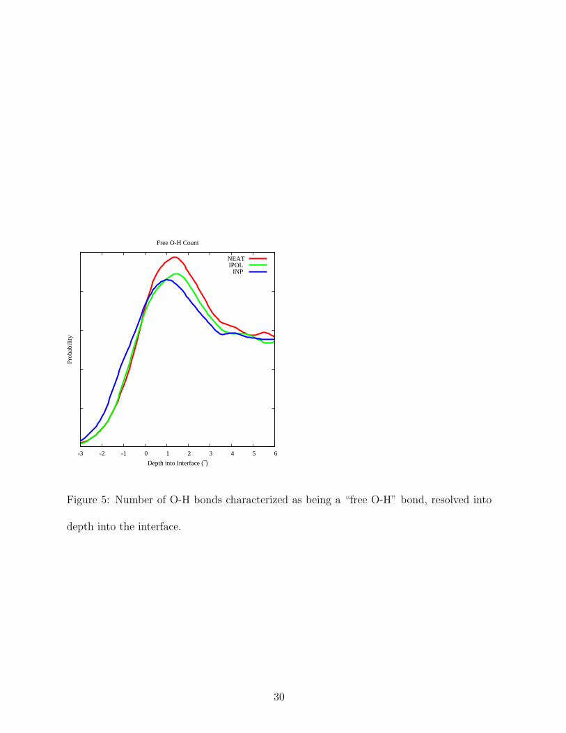
molecules which contain free O-H bond between each of the systems. As is evident in

Figure 5, there are no large differences, and hence one would not expect there to be large

differences in the SFG spectra due to a change in number density of free O-H oscillators.

14

3.2 Spectroscopy

As a way of highlighting the usefulness of SFG spectroscopy, we begin the discussion of

our spectroscopic calculations by demonstrating the limitations of IR and Raman spec-

troscopies for differentiating between the salt water solutions and the neat water system.

Because the SFG intensity arises from the quantities also required to compute the IR and

Raman spectra,[45] the latter are readily computed during the course of the computation

of the SFG spectrum.

Linear spectroscopies (e.g., IR and Raman) give rise to features corresponding to both

bulk and interfacial waters (i.e., isotropic and anisotropic environments). As expected,

there is almost no difference between the theoretical IR (Figure 6) or Raman (Figure 7)

spectra of the NEAT, IPOL and INP systems. Benjamin has pointed out that hypothetical

IR spectra of only the top-most layer can be calculated.[46] We also report these theoretical,

top-most layer IR and Raman spectra for each of the systems in Figures 6 and 7. These

spectra yield two important details: 1) the appearance of the “free O-H” oscillator as a

shoulder at ca. 3750 cm−1 and 2) the fact that there is only a small difference between the

IR and Raman spectra in terms of the relative intensities of the hydrogen bonded region

and the “free O-H” region. We conclude from these spectra that there is either not much

difference between the oscillators of the different systems, or that the spectral differences

between NEAT, IPOL, and INP are masked by bulk-like contributions.

In contrast to the linear spectroscopies, in SFG spectroscopy, bulk-like contributions

vanish, leaving only the anisotropic environments more clearly visible in the spectrum. The

15

computation of SFG spectra involves a large amount of sampling over many trajectories in

order to average the bulk-like components to zero. [22] Since these calculations are rather

time consuming, it is desireable to find a way to reduce the required effort. The ODFs

give some clue as to which regions of the bulk are anisotropic and which are isotropic.

The computed susceptibilities converge at about Z=9 A, where the ODF profiles strongly

suggest that the environment is isotropic. Therefore, the computed susceptibilities and

SFG spectra involve summation of molecules which are no more than 9 A below the Gibbs

dividing surface.

The resonant susceptibilities of NEAT, IPOL, and INP are similar in the region around

3750 cm−1 (Figure 8). However, the salt water solutions have a clear “onset” at 3300

cm−1, which gives rise to the features in the SFG spectrum corresponding to a peak max-

imum of ∼3400 cm−1. Since the main structural difference between NEAT and the salt

water interfaces (INP and IPOL) is the presence of the subsurface water ordering in the

latter systems, we attribute this feature to water oscillators which are ordered by the ion

double layer. Unfortunately, the phase information corresponding to this feature is lost

in the actual SFG spectrum, since the intensity is related to the square modulus of the

susceptibility according to eq 1. [13]

The theoretical SFG spectrum given by eq 1 involves the sum of the resonant and

nonresonant susceptibilites. Although we originally attempted to compute the frequency-

independent nonresonant susceptibility of each system following the prescription of Morita

and Hynes, the values were plagued by large statistical uncertainties and turned out to

be orders of magnitude off from what would be required to generate a reasonable SFG

16

spectrum from the simple addition of this term to the resonant contribution.[22] Therefore,

we simply chose χNR to be a real-valued, adjustable parameter which furnishes the SFG

spectra with baselines similar to the ones revealed experimentally. We investigated a range

of values for this term and there appear to be bounds in which a reasonable lineshape

and baseline are maintained. Whereas we are confident that the chosen values of the

non-resonant term yield computed SFG spectra that are “realistic,” we point out that

a weakness of this approach is that the accurate, first-principles calculation of this term

remains elusive. [22]

Figure 9 shows our computed SFG spectra (ssp polarization) for NEAT, IPOL, and

INP. The computed SFG spectra of the three systems exhibit similar features: a broad

band around 3400 cm−1 corresponding to stretching of waters in the hydrogen bonded

region, and a sharp intensity at 3750 cm−1 that corresponds to the “free O-H” stretch.

Our computed SFG spectrum for neat water is in excellent agreement with that reported

by Morita and Hynes for a somewhat smaller system. [22] The main difference between

predicted SFG spectrum of the neat water system and the predicted spectra of the salt

water systems is that in the salt water systems there is, in qualitative agreement with

experiment, a considerable increase in intensity of the region around 3400 cm−1 relative to

the “free O-H” stretch in the salt water systems.

17

4 Conclusions

Based on the results of molecular dynamics simulations, we predict that iodide ions exist

at the air/water interface with a surfactant-like excess. When polarizability is included in

the force field of the ions (IPOL), this excess is much greater than the case where the ion

polarizability is neglected (INP). This is in agreement with our previous simulations that

employed a somewhat different (i.e., polarizable, rigid) model for the water molecules.

Comparison of the time-averaged orientational distribution functions of the water dipoles

with respect to the surface-normal vector in IPOL and NEAT reveals that there is a signif-

icant subsurface ordering in IPOL that does not appear in the case of NEAT. Because the

excess ordering corresponds to an angle of ∼0◦ with respect to the surface normal vector,

and the depletion of ordering corresponds to an angle of ∼150◦, we postulate that these

deviations from time-averaged isotropic orientation are due to electrostatically favorable

(∼0◦) and electrostatically unfavorable (∼150◦) interactions of water with a time-averaged

ionic double layer. This assumption is supported by the fact that INP, which has a less-

pronounced ion double layer, also shows less subsurface water ordering than IPOL.

We have computed the theoretical SFG spectra of these systems using the approach

outlined by Morita and Hynes.[22] We have demonstrated that there is a significant en-

hancement in the SFG intensity at 3400 cm−1 upon the addition of sodium iodide. This is

in agreemeent with the experimental results of the groups of Richmond [17] and Allen. [16]

There is no significant difference in absolute intensities in the 3400 cm−1 region between

IPOL and INP, despite the stronger ion separation and water ordering in the interfacial

18

layer in the former case. The increase (vs. neat water) of the intensity of the 3400 cm−1

band relative to the 3750 cm−1 band is slightly larger in the IPOL system compared to the

INP system. Taken together, our computed spectra and structural analysis suggest that

the changes in the experimentally measured SFG spectra accompanying addition of sodium

iodide to water could be consistent with the adsorption of anions and the presence of a

diffuse double layer at the solution-air interface, with a concomitant increase in ordering

of the interfacial water molecules.

SFG spectroscopy, which directly probes the water oscillators, is an indirect probe of

the presence and structure of the ions in the interfacial layer. Moreover, quantitative

characterization of the water subsurface ordering (presumably caused by interaction with

the interfacial ion double layer) via SFG spectroscopy might be difficult due to the fact

that all phase information is lost. However, subsurface ordering is predicted to be visible

in the resonant susceptibility, which does exhibit strong sensitivity to the orientation of the

water molecules as manifested in the phase of this complex quantity. Shen and coworkers

have recently reported experimental resonant susceptibilities for aqueous systems, although

these studies involved a solid surface.[49] Alternatively, SFG spectra which employ different

polarizations (e.g., ppp) might reveal the existence of subsurface water ordering. It would be

interesting to see the results of further experiments which probe salt solution/air interfaces.

19

5 Acknowledgement

We are grateful to Prof. A. Morita, Prof. J. T. Hynes, Prof. B. J. Finlayson-Pitts, Dr. J. S.

Vieceli, and Dr. J. A. Freites for fruitful discussions. The applicability of the iterative solver

used in this work was demonstrated by Miss O. Mandelshtam and Prof. V. Mandelshtam.

Prof. H. C. Allen and Prof. G. S. Richmond are acknowledged for providing us with

their experimental SFG spectra prior to publication. All calculations were performed on

the Medium Performance Cluster at the University of California. We thank the National

Science Foundation (via the Environmental Molecular Sciences Institute) and the Czech

Ministry of Education (grant ME644) for financial support.

20

References

[1] Finlayson-Pitts, B. J.; Pitts, J. N. Chemistry of the Upper and Lower Atmosphere;

Academic Press: San Diego, 2000.

[2] Knipping, E. M.; Lakin, M. J.; Foster, K. L.; Jungwirth, P.; Tobias, D. J.; Ger-

ber, R. B.; Dabdub, D.; Finlayson-Pitts, B. J. Science 2000, 288, 301.

[3] Jungwirth, P.; Tobias, D. J. Journal of Physical Chemistry B 2002, 106, 6361.


[5] Dang, L. X. Journal of Physical Chemistry B 2002, 106, 10388.

[6] Dang, L. X.; Chang, T. M. Journal of Physical Chemistry B 2002, 106, 235.

[7] Laskin, A.; Gaspar, D. J.; Wang, W.; Hunt, S. W.; Cowin, J. P.; Colson, S. D.;

Finlayson-Pitts, B. J. Science 2003, 301, 340.

[8] Tobias, D. J.; Jungwirth, P.; Parrinello, M. Journal of Chemical Physics 2001, 114,

7036.

[9] Perera, L.; Berkowitz, M. L. Journal of Chemical Physics 1991, 95, 1954.

[10] Washburn, E. W. International Critical Tables, Volume IV; McGraw-Hill: New York,

1928.

[11] Vrbka, L.; Mucha, M.; Minofar, B.; Jungwirth, P.; Brown, E. C.; Tobias, D. J.

Current Opinon in Colloid and Interface Science 2004, 9, 67.

21

[12] Mukamel, S. Principles of Nonlinear Optical Spectroscopy; Oxford University Press:

Oxford, 1995.

[13] Shen, Y. R. . In Proceedings of the International School of Physics “Enrico Fermi”,

Vol. 120; Hansch, T.; Ingusio, M., Eds.; North-Holland: Amsterdam, 1994.

[14] Eisenthal, K. B. Chemical Reviews 1996, 96, 1343.

[15] Richmond, G. L. Chemical Reviews 2002, 102, 2693.

[16] Liu, D.; Ma, G.; Levering, L. M.; Allen, H. C. Journal of Physical Chemistry B

2004, 108, 2252.

[17] Raymond, E. A.; Richmond, G. L. Journal of Physical Chemistry B 2004, 108, 5051.

[18] Pouthier, V.; Hoang, P. N. M.; Girardet, C. Journal of Chemical Physics 1999, 110,

6963.

[19] Morita, A.; Hynes, J. T. Chemical Physics 2000, 258, 371.

[20] Brown, M. G.; Walker, D. S.; Raymond, E. A.; Richmond, G. Journal of Physical

Chemistry B 2003, 107, 237.

[21] Perry, A.; Ahlborn, H.; Space, B.; Moore, P. Journal of Chemical Physics 2003,

118, 8411.

[22] Morita, A.; Hynes, J. T. Journal of Physical Chemistry B 2002, 106, 673.

[23] Becke, A. D. Journal of Chemical Physics 1993, 98, 5648.

22

[24] Lee, C.; Yang, W.; Parr, R. G. Physical Review B 1988, 37, 785.

[25] Kendall, R.; T.H. Dunning, J.; Harrison, R. Journal of Chemical Physics 1992, 96,

6796.

[26] Dunning, T. H. Journal of Chemical Physics 1994, 100, 2975.

[27] Basis sets were obtained from the Extensible Computational Chemistry Environment

Basis Set Database, Version 02/25/04, as developed and distributed by the Molecular

Science Computing Facility, Environmental and Molecular Sciences Laboratory which

is part of the Pacific Northwest Laboratory, P.O. Box 999, Richland, Washington

99352, USA, and funded by the U.S. Department of Energy. The Pacific Northwest

Laboratory is a multi-program laboratory operated by Battelle Memorial Institute for

the U.S. Department of Energy under contract DE-AC06-76RLO 1830. Contact David

Feller or Karen Schuchardt for further information.

[28] Frisch, M. J. et al. Gaussian 03, Revision A.1 2003, Gaussian, Inc., Pittsburgh, PA.

[29] Denbigh, K. G. Transactions of the Faraday Society 1940, 36, 936.

[30] LeFevre, C. G.; LeFevre, R. J. W. Reviews in Pure and Applied Chemistry 1955, 5,

261.

[31] Miller, K. J. Journal of the American Chemical Society 1990, 112, 8543.

[32] Ferguson, D. M. Journal of Computational Chemistry 1995, 15, 501.

23

[33] Markovich, G.; Perera, L.; Berkowitz, M. L.; Cheshnovsky, O. J. Journal of Chemical

Physics 1006, 105, 2675.

[34] Case, D. A. et al. AMBER 7 2002, University of California, San Francisco.

[35] Essmann, U.; Perera, L.; Berkowitz, M. L.; Darden, T.; Petersen, L. G. Journal of

Chemical Physics 1995, 103, 8577.


[37] Thole, B. T. Chemical Physics 1981, 59, 341.

[38] van Duijnen, P. T.; Swart, M. Journal of Physical Chemistry A 1998, 102, 2399.

[39] Applequist, J.; Carl, J. R.; Fung, K.-K. Journal of the American Chemical Society

1972, 94, 2952.

[40] Silberberg, L. Phil. Mag. 1917, 33, 521.

[41] van der Vorst, H. A.; Vuik, C. Numerical Linear Algebra Applications 1994, 1, 369.

[42] Clough, S. A.; Beers, Y.; Klein, G. P.; Rothman, L. S. Journal of Chemical Physics

1973, 59, 2254.

[43] Silvestrelli, P. L.; Parrinello, M. Physical Review Letters 1999, 82, 3308.

[44] Press, W. H.; Teukolsky, S. A.; Flannery, B. P.; Vetterling, W. T. Numerical Recipes

in Fortran: The Art of Scientific Computing; Cambridge University Press: New York,

1992.

24

[45] Gordon, R. G. Advances in Magnetic Resonance 1968, 3, 1.

[46] Benjamin, I. Physical Review Letters 1994, 73, 2083.

[47] Benjamin, I. Chemical Reviews 1996, 96, 1449.

[48] Wei, X.; Shen, Y. R. Physical Review Letters 2001, 86, 4799.

[49] Shen, Y. R. Sum-frequency vibrational spectroscopy of water/quartz interfaces: Crys-

talline vs. fused quartz. In Abstracts of the American Chemical Society National Meet-

ing ; American Chemical Society: Anaheim, California, 2004.

25

Figure 1: Schematic description of the distances and angles involved in the definition of

the “free O-H” bond. The angle criterion is 30◦, and the distance criterion is 3.5 A.

26

−2 0 2 4 6 8

Pro

babi

lity

Depth into Interface (Å)

Polarizable Ions (POL)

I−

Na+

O

−2 0 2 4 6 8

Pro

babi

lity


Nonpolarizable Ions (INP)

I−

Na+

O

−2 0 2 4 6 8

Pro

babi

lity


Neat Water (NEAT)

O

Figure 2: Density profiles of IPOL (left panel), INP (center panel), and NEAT (right

panel). Zero on the x-axis corresponds to the Gibbs dividing surface.

27

0 0.2 0.4 0.6 0.8 1 1.2 1.4 1.6 1.8

Polarizable Ions (IPOL)

0 1 2 3 4 5 6Depth into Interface (Å)

−1

−0.5

0

0.5

1

P(cos θ)

0 0.2 0.4 0.6 0.8 1 1.2 1.4 1.6 1.8



−1

−0.5

0

0.5

1

P(cos θ)

0 0.2 0.4 0.6 0.8 1 1.2 1.4 1.6 1.8

Neat Water (NEAT)


−1

−0.5

0

0.5

1

P(cos θ)

Figure 3: Orientational distribution functions as a function of depth into the interface. The

values have been scaled such that a unit value corresponds to an isotropic environment.

28

−0.6

−0.4

−0.2

0

0.2

0.4

0.6



−1

−0.5

0

0.5

1

P(cos θ)

−0.6

−0.4

−0.2

0

0.2

0.4

0.6



−1

−0.5

0

0.5

1

P(cos θ)

Figure 4: Orientational distribution functions of IPOL and INP, less the ODF profile of

NEAT.

29

-3 -2 -1 0 1 2 3 4 5 6

Prob

abili

ty

Depth into Interface (¯)

Free O-H Count

NEATIPOL

INP

Figure 5: Number of O-H bonds characterized as being a “free O-H” bond, resolved into

depth into the interface.

30

3000 3200 3400 3600 3800 4000

Inte

nsity

(ar

b. u

nits

)

Frequency (cm−1)

Theoretical Infrared Spectrum − Bulk

NEATINP

IPOL

3000 3200 3400 3600 3800 4000

Inte

nsity

(ar

b. u

nits

)

Frequency (cm−1)

Theoretical Infrared Spectrum − Surface

NEATINP

IPOL

Figure 6: Theoretical infrared spectrum of the bulk (left panel) and topmost layer (Z <

0) of IPOL, INP, and NEAT.

31

3000 3200 3400 3600 3800 4000

Inte

nsity

(ar

b. u

nits

)

Frequency (cm−1)

Theoretical Raman Spectra − Bulk

NEATINP

IPOL

3000 3200 3400 3600 3800 4000

Inte

nsity

(ar

b. u

nits

)

Frequency (cm−1)

Theoretical Raman Spectra − Surface

NEATINP

IPOL

Figure 7: Theoretical infrared spectrum of the bulk (left panel) and topmost layer (Z <

0) of IPOL, INP, and NEAT.

32

3000 3200 3400 3600 3800 4000

Inte

nsity

(a.

u.)

Frequency (cm−1)


ReIm

3000 3200 3400 3600 3800 4000

Inte

nsity

(a.

u.)

Frequency (cm−1)


ReIm

3000 3200 3400 3600 3800 4000

Inte

nsity

(a.

u.)

Frequency (cm−1)

Neat Water (NEAT)

ReIm

Figure 8: Theoretical resonant susceptibilities (xxz, yyz) of IPOL (left panel), INP (center

panel), and NEAT (right panel).

33

3000 3200 3400 3600 3800 4000

Inte

nsity

(ar

bitr

ay u

nits

)

Frequency (cm−1)

SFG Spectrum (ssp)

NEATIPOL

INP

Figure 9: Theoretical vibrational Sum Frequency Generation spectrum (ssp) of IPOL, INP,

and NEAT.

34

structure and vibrational spectroscopy of salt water/air...

Documents