1

Structure of Speech

• Physical acoustics– Time-domain representation– Frequency domain representation– Sound shaping

• Speech acoustics– Source-Filter Theory– Speech Source characteristics– Speech Filter characteristics

• Acoustic Phonetics– Classification and Features– Segmental structure– Coarticulation– Suprasegmentals

Physical acoustics pertains to what sound is and how it is described. Mostsimply, sound is the propagation of pressure variations through a medium suchas air, water, train rails, etc. We cover the representation of sound in the time-domain as the time course of pressure variations, and in the frequency domainas the ampli tude and phase of one or more sinusoids. We draw a distinctionbetween sound sources (things that generate sound by vibrating), and waysound is altered by the acoustic properties of objects it interacts with such asresonating tubes.

Physical acoustics provides the background to understand how speech soundsare generated and controlled by the vocal tract and articulators. The discussionof speech acoustics is primarily about speech production.

Finally, we will examine the relationship between the linguistic characteristicsof speech and the structure of the acoustic speech signal. This will i ncludediscussion of segments or phonemes (corresponding roughly to vowels andconsonants), sub-phonemic acoustic features of speech such as voicing,manner, place that can be used to characterize phonemes, as well as propertiesthat extend over several phonemes or even an entire utterance.

2

Physical Acoustics: Time-domain

• Simple waveforms– Amplitude, Frequency, and Phase– Physical versus perceptual characteristics

• Complex waveforms• Periodic and aperiodic waveforms

Simple waveforms are sinusoidal signals that are completely described by theiramplitude, frequency, and phase. Amplitude describes the degree offluctuation in pressure, frequency is the number of pressure fluctuations perunit time, and phase is the relative alignment of the pressure fluctuations withrespect to a specific instant.

Perceptually, amplitude corresponds to loudness of a sound, and frequency toits pitch. Under most conditions, phase is not perceptually significant. Therelationship between changes in loudness/pitch and changes inamplitude/frequency is roughly logarithmic. That is, at lowamplitudes/frequencies, small changes result in large perceived changes inloudness or pitch, while at high amplitudes/frequencies much largeramplitude/frequency changes are needed to produce the same perceivedchange in loudness or pitch.

Complex waveforms contain multiple sinusoidal (simple) waveforms.

Sinusoids are periodic. Each cycle of a sinusoid is repeated exactly in the nextcycle. Complex waveforms may also be periodic if they contain cyclic patternsthat repeat exactly. Aperiodic waveforms are complex waveforms that do notcontain cyclic patterns that repeat exactly. Many biological and other real-world signals--including the speech signal--may contain sequences of verysimilar patterns that are nearly but not exactly the same. Such sounds aresimilar to periodic sounds and are called quasiperiodic.

3

Simple Waveform

( )sff2sin iayi πθ +×=

a = Amplitudeθ = Phasef = Frequencyfs = Sampling Rate

For all integer i:

NOTES:

1) By definition, simple waveforms are sinusoids. Any sinusoid can becompletely specified by three parameters:

•Amplitude (a) - The extent of pressure variation.

•Frequency (f) - The rate of pressure variation in terms of the numberof complete cycles of the sinusoid per second (Hertz abbreviated Hz).

•Phase (θ)- An offset of the function with respect to a specific time.

2) Although we are technically dealing with analog signals, this is obviously adiscrete approximation to a sine function with an additional parameter, thesampling rate (fs). For frequency specified in Hz, fs is the number of equallyspaced instants every second at which the function is evaluated.

4

Simple Waveforms

175 Hz225 Hz275 Hz325 Hz375 Hz425 Hz475 Hz

NOTES:

1) Here are several sinusoids illustrating variations both frequency, amplitude,and phase. These are orthogonal (each can be varied independently of theothers), but not in these diagrams where the top right frame is both lower inamplitude and higher in frequency than the top left.

2) The three graphs are:

•Top left - 200 Hz tone.

•Top right - 600 Hz tone at lower amplitude.

•Bottom left - two 200 Hz tones of the same amplitude differing inphase

3) It is worthwhile noting that the physical features frequency and amplitudecorrespond to the perceptual features of pitch and loudness respectively, butthe relationships between physical and perceptual features are not linear. Therelationship is roughly logarithmic: small physical changes at lowfrequencies/amplitudes are perceptually much larger than equal physicalchanges at high frequencies/amplitudes.

This is ill ustrated in the sounds linked to the buttons on the bottom right - Allsteps are 50 Hz, but the pitch difference between 175 and 225 Hz is greaterthan the pitch difference between 425 and 475 Hz. [I don’ t know how to makethis link work in a PDF file - HTB]

5

Complex waveforms

( )∑=

+×=K

0kskkk ff2sin iayi πθ

ak = Ampli tude of kth componentθκ = Phase of kth componentfk = Frequency of kth componentfs = Sampling Rate

For all integer i: For all integer k | (0 < k < K):

NOTES:

1) Complex waveforms can be described as the summation of a series of twoor more simple waveforms.

2) In the discrete but unbounded case, K = ∞. Later, we wil l explore theconsequences of using finite i and K.

6

Complex Waveforms

NOTES:

1) This figure shows three complex waveforms, and one simple waveform. Itshows how non-sinusoidal functions of time can be approximated by summingsimple waveforms of the correct frequencies, amplitudes, and phases.

2) Graphs in the figure are:

•Top left - 200 Hz Square wave

•Top right - 200 Hz Sine wave is first component of the square wave(NOT a complex wave, but the first in the series of simple waves thatsum to form a square wave. This is called the fundamental frequencyand is typically written as F0.

•Bottom left - 200 Hz Sine wave + 600 Hz Sine wave. The 600 Hz sinewave (at three times F0) is 1/3 the amplitude of F0 and has the samephase. Components at integer multiples of F0 are called harmonics.

•Bottom right - Sum of sine waves at 200, 600, 1000, 1400 Hz. Thesefrequencies correspond to F0 and its 3rd, 5th, and 7th harmonics. Theamplitudes of these are 1/3, 1/5, and 1/7 the ampli tude of the F0component. All have the same phase.

3) Perceptually, all of these signals would have the same pitch, correspondingto that of a 200 Hz sine wave, but timbre differs, becoming brighter as morecomponents are combined.

7

Aperiodic Waveforms

Impulse - only non-zerofor one instant.

Random - Amplitudevariations are withouttemporal structure.

NOTES:

1) All the previous waveforms we’ve examined are called periodic becausethey consist of a basic pattern (however complex) that repeats over time. Thelength of the pattern (called its period) is inversely related to the fundamentalfrequency of the periodic waveform and all the sinusoidal components neededto describe the structure of the waveform will fall at integer multiples of F0.The period (P) of a waveform is thus specified by the relation P = 1/F0.

2) These examples of aperiodic waveforms differ from periodic waveforms inthat they do not have a repeating temporal pattern.

3) The impulse is (theoretically) non-zero at only one instant and zero at allother instants.

4) A waveform with random amplitude also lacks systematic repetition ofamplitude values over time (if the random number generator is any good).

8

Physical Acoustics: Frequency-domain

• Line spectra– Represent periodic signals– One or more sinusoids that are harmonically related– Harmonics can appear only at frequencies that are

integer multiples of the fundamental (usually lowest)frequency.

• Continuous spectra– Represent aperiodic signals– Energy present (potentially) at any frequency, not just

harmonically related frequencies.

NOTES:

1) The frequency domain and time domain are alternative representations ofexactly the same signals. Conversion between the two is informationpreserving.

9

Line Spectra

NOTES:1) These figures make it clear why we refer to the spectra of periodic signals as line spectra.There can be information in the spectrum only at the fundamental frequency (F0) and itsinteger multiples.

2) We have left something out of these diagrams: there is no phase information displayed. Itcould be if we added a Y-Z plane as a 3rd dimension to the figures. We could then show phaseas a rotation angle of the line around the X axis in the Y-Z plane. However, to a firstapproximation, we are unable to perceive phase relations in complex signals and it is thusnormal practice to display the magnitude only of components (lines), disregarding their phase.

3) The figure at the top left is from a simple waveform (i.e., one sinusoid). It has a frequencyof 0.20 kHz (that kilo Hertz) or in other words, 200 Hz. It’ s amplitude is 100 on a scale ofunspecified units.

4) The top right figure is the spectrum of a 200 Hz square wave. Note that it has lines atfrequencies and ampli tudes that correspond to the components we previously added toapproximate the square wave.

5) The bottom left figure is the same spectrum shown in the top right, but with logarithmicunits of ampli tude instead of linear units. Specifically, amplitude is shown in decibels (dB).Conversion from linear amplitude units to dB follows the relation: dB = 20.0 * log10(amp/ref)where amp is the linear amplitude and ref is a reference amplitude for sound in air, thereference is 0.002 dyne. For digitized speech, the ref is commonly a unit amplitude step.

10

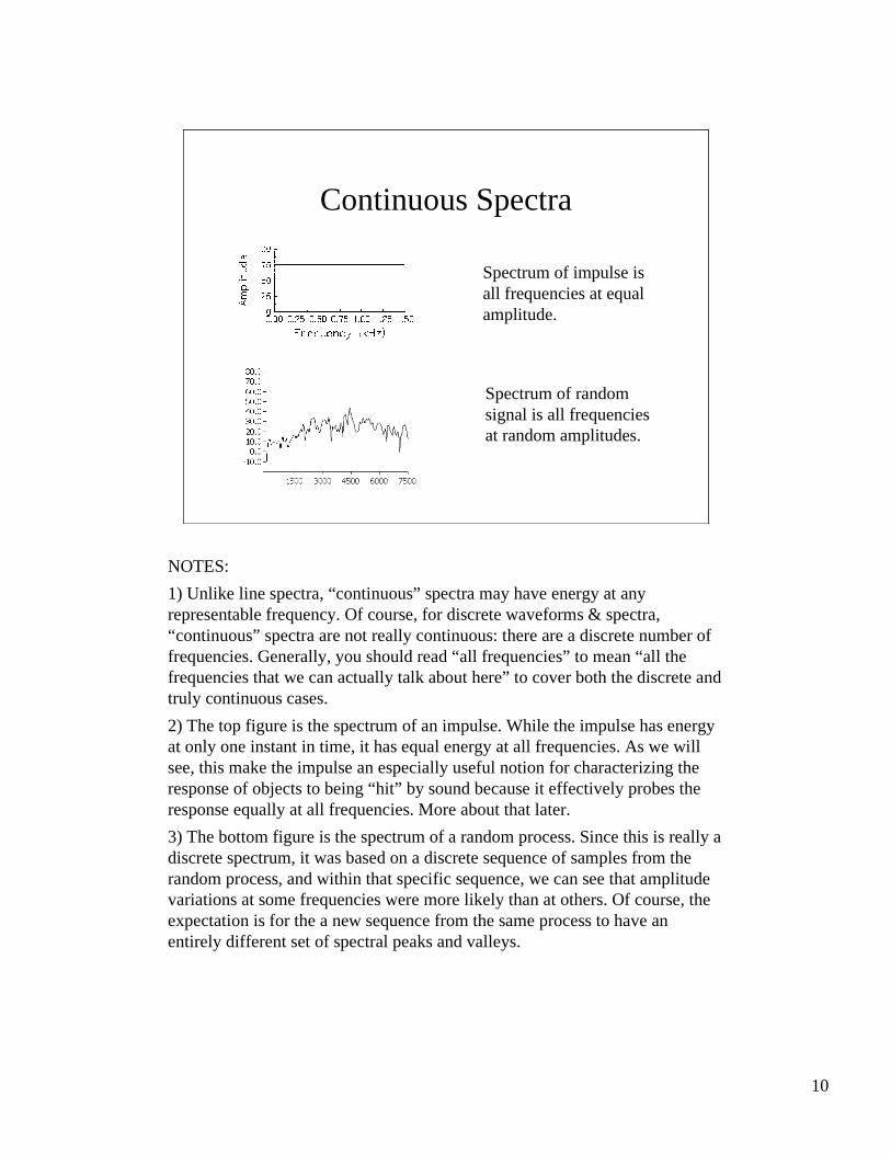
Continuous Spectra

Spectrum of impulse isall frequencies at equalamplitude.

Spectrum of randomsignal is all frequenciesat random amplitudes.

NOTES:

1) Unlike line spectra, “continuous” spectra may have energy at anyrepresentable frequency. Of course, for discrete waveforms & spectra,“continuous” spectra are not really continuous: there are a discrete number offrequencies. Generally, you should read “all frequencies” to mean “all thefrequencies that we can actually talk about here” to cover both the discrete andtruly continuous cases.

2) The top figure is the spectrum of an impulse. While the impulse has energyat only one instant in time, it has equal energy at all frequencies. As we willsee, this make the impulse an especially useful notion for characterizing theresponse of objects to being “hit” by sound because it effectively probes theresponse equally at all frequencies. More about that later.

3) The bottom figure is the spectrum of a random process. Since this is really adiscrete spectrum, it was based on a discrete sequence of samples from therandom process, and within that specific sequence, we can see that amplitudevariations at some frequencies were more likely than at others. Of course, theexpectation is for the a new sequence from the same process to have anentirely different set of spectral peaks and valleys.

11

Quasiperiodicity

Log magnitude of asquare wave

Log magnitude of ajittery square wave

NOTES:

1) The top figure is the log magnitude spectrum of the square wave we werejust looking at.

2) The bottom figure is also the spectrum of a square wave, but with onesignificant difference. In this case, the square wave was “windowed” over alarge number of cycles to begin at zero amplitude, grow to a maximumamplitude and then decrease back to zero ampli tude again. This is now anamplitude modulated square wave and because every cycle is not exactly likeevery other cycle, it is no longer periodic, but it is nearly so.This is calledquasiperiodic.

3) Quasiperiodic signals give rise to spectra that are similar to line spectrawhere the lines have measurable width. Such spectra are technicallycontinuous spectra, not line spectra.

4) Because quasiperiodic signals are the rule rather than the exception in thereal world, we refer to spectra produced by such signals as harmonic spectra.

5) The individual wide lines in harmonic spectra are called harmonics of F0just as lines are in the pure line spectrum case.

12

Physical Acoustics: Soundshaping

• Sources– Generators of sound energy– Periodic or aperiodic– possibly complex temporal/spectral structure

• Filters– Low pass– High pass– Band pass

• Resonance– Pendulums– Tubes– Frequency domain properties

NOTES:

1) All sound must originate with an energy source driving an object andmaking it vibrate. The structure of the sound emanating from the vibratingobject (its waveform or spectrum) will be a function of two things: thestructure (movement pattern) of the driving source, and the way that the objectbeing driven responds to being vibrated.

2) Sound itself may be the energy source that is striking an object and makingit vibrate. In such instances, the final “output” sound of the object will be dueto both the structure of the original driving sound and the manner in which theobject responds to being driven.

3) If we know the response characteristics of the object being driven and thestructure of the driving force (whatever it is), we can determine what theoutput of the system comprising the driving force and driven object wil l be.This is the case for a particular class of “driven objects,” fil ters, andresonators, that we’ ll discuss next.

4) Filters respond to a source function by attenuating the energy of the sourceat some frequencies. Typical classes of filters will be discussed in the nextslide.

5) Unlike filters, resonators have a specific frequency at which they prefer tovibrate called their resonant frequency. It takes very littl e energy to produce aresponse at the resonant frequency and the response will continue for sometime after the driving source is removed.

13

FiltersA

mpl

itud

e (d

B)

Frequency

Low pass High pass Band pass

0 0 0-3 -3-3

Bandwidth

NOTES

1) These are three fundamental types of filters. Shown in the frequencydomain. Other more complicated filters could be constructed by combiningeffects of simple filters. The axes for the three diagrams are arbitraryfrequency (X axis) and arbitrary amplitude (Y axis) scales.

2) Filters are most simply characterized by their bandwidth and slope.Bandwidth is the range of frequencies that pass through the filter with li ttle orno attenuation. The bandwidth of a filter is delimited by the fil ter cutofffrequency(ies), the point at which attenuation becomes greater than 3 dB.Fil ter slope is how rapidly attenuation increases after the cutoff frequency(commonly specified in dB per octave). Band pass filters are additionallycharacterized by their center frequency.

3) Low pass filters are smoothing filters. They remove rapid fluctuations in atime series while retaining larger scale features.

4) High pass filters are differentiators. They remove slow changes in a timeseries while retaining rapid changes.

5) Band pass filters are tuned to a specific frequency or range of frequenciesand reject variations outside that range.

6) The impulse response of a filter shows how it responds over time to beingexcited by an impulse. The frequency response of a filter is the fouriertransform of its impulse response, and vice versa.

14

Pendulum

0-1 +1

0

p

Tim

e

Amplitude

NOTES

1) Pendulums have a natural frequency that depends upon the length of thependulum.

2) As long as a pendulum is in free motion, it will swing at its naturalfrequency.

3) A hard push makes the pendulum swing further (greater amplitude), but willnot change the period of the swinging. That is, no matter how great theamplitude of swinging, the time required to complete one cycle of swinging isa constant.

15

Resonating Tube

Openend

Closedend

17 cm

R1 = s/4L = 34000/68 = 500R2 = 3s/4L = 1500R3 = 5s/4L = 2500etc..

NOTES

1) A uniform tube, open at one end and closed at the other resonates atfrequencies given by a quarter wavelength law: The length of the tube is 1/4ththe wavelength of the tube’s first resonant frequency.

2) The speed of sound is roughly 34 cm/msec or 34000 cm/sec. So a 17 cmtube would have its first resonance at about 500 Hz.

3) Subsequent resonances fall at odd multiples of the first resonance.

4) For tubes that are not of uniform cross sectional area, resonances differ fromthose of a uniform tube. For instance, if the front half of the tube (toward theopen end) is wider than the back half of the tube, R1 will be higher infrequency, R2 lower in frequency, R3 higher in frequency, R4 lower, and soforth. The greater the difference in area, the greater the effect on resonantfrequencies.

16

Resonators

-60

-50

-40

-30

-20

-10

0

10

20

30

40

0 1000 2000 3000 4000 5000 6000 7000 8000 9000

Frequency (Hz)

Am

plit

ud

e (d

B)

50015003500

NOTES

1) This figure shows the frequency response of three resonators each with abandwidth of 100 Hz but with resonant frequencies of 500, 1500, and 3500 Hz.The magnitude of their response (in dB) is plotted relative to energy input tothe resonator.

2) Resonators share some properties of band pass filters in that they can becharacterized by their center frequency--more accurately their resonant ornatural frequency--and their bandwidth.

3) Unlike filters, resonators have greater than 0 dB response in theneighborhood of their natural frequency. This means that the energy out of theresonator is actually greater than the driving energy into the resonator in thisregion.

4) For resonators, the narrower the bandwidth, the greater the response is at theresonant frequency.

5) For resonators of equal bandwidth, the greater the resonant frequency, thegreater the response level at the resonant frequency and all frequencies abovethe resonant frequency.

6) This last fact has implications for speech where we see that the higher thefrequency of the first resonance of the vocal track, the greater the overallamplitude of the speech signal.