structure-preserving, energy stable numerical schemes for

Copyright © by SIAM. Unauthorized reproduction of this article is prohibited.

SIAM J. SCI. COMPUT. © 2021 Society for Industrial and Applied MathematicsVol. 43, No. 2, pp. A1248--A1272

STRUCTURE-PRESERVING, ENERGY STABLE NUMERICALSCHEMES FOR A LIQUID THIN FILM COARSENING MODEL\ast

JUAN ZHANG\dagger , CHENG WANG\ddagger , STEVEN M. WISE\S , AND ZHENGRU ZHANG\P

Abstract. In this paper, two finite difference numerical schemes are proposed and analyzedfor the droplet liquid film model with a singular Lennard--Jones energy potential involved. Bothfirst and second order accurate temporal algorithms are considered. In the first order scheme, theconvex potential and the surface diffusion terms are updated implicitly, while the concave potentialterm is updated explicitly. Furthermore, we provide a theoretical justification that this numericalalgorithm has a unique solution such that the positivity is always preserved for the phase variable ata pointwise level, so that a singularity is avoided in the scheme. In fact, the singular nature of theLennard--Jones potential term around the value of 0 prevents the numerical solution reaching sucha singular value, so that the positivity structure is always preserved. Moreover, an unconditionalenergy stability of the numerical scheme is derived, without any restriction for the time step size. Inthe second order numerical scheme, the BDF temporal stencil is applied, and an alternate convex-concave decomposition is derived, so that the concave part corresponds to a quadratic energy. Inturn, the combined Lennard--Jones potential term is treated implicitly, and the concave part isapproximated by a second order Adams--Bashforth explicit extrapolation, and an artificial Douglas--Dupont regularization term is added to ensure the energy stability. The unique solvability andthe positivity-preserving property for the second order scheme could be similarly established. Inaddition, optimal rate convergence analysis is provided for both the first and second order accurateschemes. A few numerical simulation results are also presented, which demonstrate the robustnessof the numerical schemes.

Key words. droplet liquid film model, unique solvability, positivity-preserving, energy stability,optimal rate convergence analysis

AMS subject classifications. 35K35, 35K55, 49J40, 65M06, 65M12

DOI. 10.1137/20M1375656

1. Introduction. Certain liquids on a solid, chemo-attractive substrate sponta-neously form a droplet structure connected by a very thin precursor (or wetting) layer.After the droplets appear, coarsening will occur, whereby smaller droplets will shrinkand larger droplets will grow. The coarsening behavior of droplets, especially the rateof coarsening, has been of great scientific interest. The average droplet size increaseswith the decrease of the number of droplets and the increase of the characteristicdistance. The coarsening process can be mediated by two mechanisms: collapse orcollision. Collapse occurs through mass exchange between droplets in the precur-

\ast Submitted to the journal's Methods and Algorithms for Scientific Computing section October 26,2020; accepted for publication (in revised form) December 18, 2020; published electronically April 8,2021.

https://doi.org/10.1137/20M1375656Funding: The work of the second author was partially supported by the National Science

Foundation (USA) through grant NSF DMS-2012669. The work of the third author was partiallysupported by the NSF through grants DMS-1719854 and DMS-2012634. The work of the fourthauthor was supported by the National Natural Science Foundation of China (NSFC) through grants11871105 and 11571045, and by the Science Challenge Project TZ2018002.

\dagger School of Mathematical Sciences, Beijing Normal University, Beijing 100875, People's Republicof China ([email protected]).

\ddagger Corresponding author. Department of Mathematics, The University of Massachusetts, NorthDartmouth, MA 02747-2300 USA ([email protected]).

\S Department of Mathematics, The University of Tennessee, Knoxville, TN 37996 USA ([email protected]).

\P Laboratory of Mathematics and Complex Systems, Beijing Normal University, Beijing 100875,People's Republic of China ([email protected]).

A1248

Dow

nloa

ded

04/1

5/21

to 2

19.1

42.9

9.11

. Red

istr

ibut

ion

subj

ect t

o SI

AM

lice

nse

or c

opyr

ight

; see

http

s://e

pubs

.sia

m.o

rg/p

age/

term

s

https://doi.org/10.1137/20M1375656

mailto:[email protected]






ENERGY STABLE SCHEMES FOR A LIQUID THIN FILM MODEL A1249

sor/wetting layer; the droplets can also drift and collide with each other like particlesin the traditional Ostwald ripening process. Thin layers of viscous liquid are welldescribed by the lubrication approximation, which capitalizes on the separation ofhorizontal and vertical length scales. Under the assumption that the liquid film doesnot evaporate, lubrication theory leads to a single equation for the height function,\phi = \phi (x, t) > 0, of a time-dependent film [36] in the form of an H - 1 gradient flow:

\partial t\phi = \nabla \cdot (\scrM (\phi )\nabla \delta \phi F ) .

Here F is the free energy of the film/substrate system and is given by

F (\phi ) =

\int \Omega

\biggl( 1

2| \nabla \phi | 2 + \scrU (\phi )

\biggr) dx,

and the term \delta \phi F is the variational derivative of F . Specifically, the gradient term de-scribes the linearized contribution of the liquid-air surface tension, while \scrU (\phi ) modelsthe intermolecular forces between the substrate and the film. See the related researchon the coarsening dynamics [1, 2, 3, 4, 5, 21, 22, 26, 27, 28, 32, 33, 37, 38, 39, 41, 42].

In this paper, we consider a well-known Lennard--Jones-type potential [25], whichis expressed as \scrU (\phi ) = 1

3\phi - 8 - 4

3\phi - 2. Other potentials are also physically relevant [39].

The free energy is

(1.1) F (\phi ) =

\int \Omega

\biggl( 1

3\phi - 8 - 4

3\phi - 2 +

\varepsilon 2

2| \nabla \phi | 2

\biggr) dx,

where \Omega \subset \BbbR 3 is a bounded domain. The H - 1 gradient flow associated with the givenfree energy functional (1.1) with constant mobility \scrM \equiv 1 (the nonconstant mobilitycase could be handled in a similar way) is

(1.2) \partial t\phi = \Delta \mu , \mu := \delta \phi F = - 8

3(\phi - 9 - \phi - 3) - \varepsilon 2\Delta \phi .

Mass is conserved, and due to the gradient structure, the following energy dissipationlaw is formally available:

d

dtF (\phi (t)) = -

\int \Omega

| \nabla \mu | 2 dx \leq 0.

For simplicity of presentation, we assume periodic boundary conditions hold over therectangular domain \Omega . Other types of boundary conditions, such as homogeneousNeumann, can also be handled.

Some numerical simulation results have been reported for the droplet liquid filmmodel [21, 36], while the numerical analysis for this model has been very limited. Thehighly nonlinear and highly singular nature of the Lennard--Jones potential makes theequation very challenging at both the analytic and numerical levels. In particular,the structure of the potential function requires that the phase variable has to keep afixed sign, i.e., being either positive or negative, to avoid a singularity. A positivity-preserving structure is required for the numerical scheme and for physical reality.The theoretical justification of such a property, in addition to the energy dissipationproperty, turns out to be a major difficulty for the numerical analysis. Moreover, aconvergence analysis for any numerical scheme for the liquid film equation (1.2) hasalso been a long-standing open problem.

Dow

nloa

ded

04/1

5/21

to 2

19.1

42.9

9.11

. Red

istr

ibut

ion

subj

ect t

o SI

AM

lice

nse

or c

opyr

ight

; see

http

s://e

pubs

.sia

m.o

rg/p

age/

term

s


A1250 J. ZHANG, C. WANG, S. M. WISE, AND Z. ZHANG

In this paper we construct and analyze finite difference numerical schemes thatpreserve all three of these important theoretical features in both the first and secondorder temporal accuracy orders. In the first order scheme, we make use of the convex-concave decomposition of the physical energy, and come up with a semi-implicit nu-merical method. The positivity-preserving property will be theoretically established,which is based on the subtle fact that the numerical solution is equivalent to a min-imization of a convex energy functional; the singular nature of the \phi - 8 term aroundthe value of 0 prevents the numerical solution reaching the singular value. As a result,the positivity structure is always preserved, and the unique solvability analysis comesfrom the convex nature of the implicit parts in the scheme. The energy stabilitybecomes a direct consequence of this convexity analysis. In the second order numeri-cal scheme, we have to make use of an alternate convex-concave decomposition of thephysical energy by observing that 1

3\phi - 8 - 4

3\phi - 2+ 4

3A0\phi 2 is a convex function provided

A0 is sufficiently large. In turn, the concave part becomes a quadratic energy, whichis approximated by a second order Adams--Bashforth explicit extrapolation. The sec-ond order backward differentiation formula (BDF) temporal stencil is applied, and anartificial Douglas--Dupont regularization term is added to ensure energy stability.

In addition, a detailed convergence analysis of the proposed numerical schemes,including the first and second order accurate ones, will be derived in this paper.This analysis gives an optimal rate error estimate in the \ell \infty (0, T ;H - 1

h )\cap \ell 2(0, T ;H1h).

A key point in the analysis lies in the following fact: since the nonlinear potentialterm corresponds to a convex energy, the corresponding nonlinear error inner productis always nonnegative. Furthermore, the error estimate associated with the surfacediffusion term indicates an \ell 2(0, T ;H1

h) convergence. This will be the first such workfor this model.

The rest of this paper is organized as follows. In section 2, we describe thefinite difference discretization of space and recall some basic facts. In section 3,we propose the first order numerical scheme and state the main theoretical results,including positivity-preserving, unique solvability, and unconditional energy stabilityof the scheme. Further, we provide a detailed convergence analysis. The secondorder accurate scheme is proposed in section 4; the unique solvability, the positivity-preserving property, and an optimal rate convergence analysis are established as well,using similar ideas. Some numerical simulation results are presented in section 5.Finally, the concluding remarks are given in section 6.

2. Finite difference spatial discretization. The model described above isinherently two-dimensional (2D) in nature. However, other models of this type maybe three-dimensional (3D). Our analyses that follow, therefore, will generically coverone through three space dimensions. For spatial approximation we use a staggered-grid finite difference approach. We use the notation and results for some discretefunctions and operators from [23, 44, 45], etc. Let \Omega = (0, Lx) \times (0, Ly) \times (0, Lz),where for simplicity, we assume Lx = Ly = Lz =: L > 0. Let N \in \BbbN be given, anddefine the grid spacing h := L

N , i.e., a uniform mesh assumption is made for simplicityof notation. We define the following two uniform, infinite grids with spacing h > 0:C := \{ pi | i \in \BbbZ \} and E := \{ pi+1/2 | i \in \BbbZ \} , where pi = p(i) := (i - 1/2)h. Considerthe following 3D discrete periodic function spaces:

\scrC per := \{ \upsilon : C \times C \times C \rightarrow \BbbR | \upsilon i,j,k = \upsilon i+\alpha N,j+\beta N,k+\gamma N \forall i, j, k, \alpha , \beta , \gamma \in \BbbZ , \} ,

\scrE xper :=

\Bigl\{ \upsilon : E \times C \times C \rightarrow \BbbR

\bigm| \bigm| \bigm| \upsilon i+ 12 ,j,k

= \upsilon i+ 12+\alpha N,j+\beta N,k+\gamma N \forall i, j, k, \alpha , \beta , \gamma \in \BbbZ

\Bigr\} ,

Dow

nloa

ded

04/1

5/21

to 2

19.1

42.9

9.11

. Red

istr

ibut

ion

subj

ect t

o SI

AM

lice

nse

or c

opyr

ight

; see

http

s://e

pubs

.sia

m.o

rg/p

age/

term

s



with the identification \upsilon i,j,k = \upsilon (pi, pj , pk), et cetera. The spaces \scrE yper and \scrE z

per areanalogously defined. The functions of \scrC per are called cell-centered functions, and thefunctions of \scrE x

per, \scrE yper, and \scrE z

per called face-centered functions. We also introduce the

following mean zero space to facilitate the later analysis: \r \scrC per := \{ \upsilon \in \scrC per | 0 = \upsilon :=h3

| \Omega | \sum N

i,j,k=1 \upsilon i,j,k\} . We define \vec{}\scrE per := \scrE xper \times \scrE y

per \times \scrE zper.

The center-to-face difference and averaging operators, Ax, Dx : \scrC per \rightarrow \scrE xper,

Ay, Dy : \scrC per \rightarrow \scrE yper, and Az, Dz : \scrC per \rightarrow \scrE z

per, are defined as follows:

Ax\upsilon i+ 12 ,j,k

:=1

2(\upsilon i+1,j,k + \upsilon i,j,k), Dx\upsilon i+ 1

2 ,j,k:=

1

h(\upsilon i+1,j,k - \upsilon i,j,k),

Ay\upsilon i,j+ 12 ,k

:=1

2(\upsilon i,j+1,k + \upsilon i,j,k), Dy\upsilon i,j+ 1

2 ,k:=

1

h(\upsilon i,j+1,k - \upsilon i,j,k),

Az\upsilon i,j,k+ 12:=

1

2(\upsilon i,j,k+1 + \upsilon i,j,k), Dz\upsilon i,j,k+ 1

2:=

1

h(\upsilon i,j,k+1 - \upsilon i,j,k).

Likewise, the face-to-center difference and averaging operators, ax, dx : \scrE xper \rightarrow \scrC per,

ay, dy : \scrE yper \rightarrow \scrC per, and az, dz : \scrE z

per \rightarrow \scrC per, are defined as follows:

ax\upsilon i,j,k :=1

2(\upsilon i+ 1

2 ,j,k+ \upsilon i - 1

2 ,j,k), dx\upsilon i,j,k :=

1

h(\upsilon i+ 1

2 ,j,k - \upsilon i - 1

2 ,j,k),

ay\upsilon i,j,k :=1

2(\upsilon i,j+ 1

2 ,k+ \upsilon i,j - 1

2 ,k), dy\upsilon i,j,k :=

1

h(\upsilon i,j+ 1

2 ,k - \upsilon i,j - 1

2 ,k),

az\upsilon i,j,k :=1

2(\upsilon i,j,k+ 1

2+ \upsilon i,j,k - 1

2), dz\upsilon i,j,k :=

1

h(\upsilon i,j,k+ 1

2 - \upsilon i,j,k - 1

2).

The discrete gradient \nabla h : \scrC per \rightarrow \vec{}\scrE per and the discrete divergence \nabla h\cdot : \vec{}\scrE per \rightarrow \scrC perare defined via

\nabla h\upsilon i,j,k :=\Bigl( Dx\upsilon i+ 1

2 ,j,k, Dy\upsilon i,j+ 1

2 ,k, Dz\upsilon i,j,k+ 1

2

\Bigr) ,

\nabla h \cdot \vec{}fi,j,k := dxfxi,j,k + dyf

yi,j,k + dzf

zi,j,k,

where \upsilon \in \scrC per and \vec{}f = (fx, fy, fz) \in \vec{}\scrE per. The standard 3D discrete Laplacian,\Delta h : \scrC per \rightarrow \scrC per, is given by

\Delta h\upsilon i,j,k : = dx(Dxv)i,j,k + dy(Dyv)i,j,k + dz(Dzv)i,j,k

=1

h2(\upsilon i+1,j,k + \upsilon i - 1,j,k + \upsilon i,j+1,k + \upsilon i,j - 1,k + \upsilon i,j,k+1 + \upsilon i,j,k - 1 - 6\upsilon i,j,k).

More generally, if \scrD is a periodic scalar function that is defined at all of the facecenter points and if \vec{}f = (fx, fy, fz) \in \vec{}\scrE per, then \scrD \vec{}f = (fx, fy, fz) \in \vec{}\scrE per, assumingpointwise multiplication; we may define

\nabla h \cdot (\scrD \vec{}f)i,j,k := dx(\scrD fx)i,j,k + dy(\scrD fy)i,j,k + dz(\scrD fz)i,j,k).

Specifically, if \upsilon \in \scrC per, then \nabla h \cdot (\scrD \nabla h) : \scrC per \rightarrow \scrC per is defined pointwise via

\nabla h \cdot (\scrD \nabla h\upsilon )i,j,k = dx(\scrD Dx\upsilon )i,j,k + dy(\scrD Dy\upsilon )i,j,k + dz(\scrD Dz\upsilon )i,j,k.

Dow

nloa

ded

04/1

5/21

to 2

19.1

42.9

9.11

. Red

istr

ibut

ion

subj

ect t

o SI

AM

lice

nse

or c

opyr

ight

; see

http

s://e

pubs

.sia

m.o

rg/p

age/

term

s



Now we are ready to define the following grid inner products:

\langle \upsilon , \xi \rangle \Omega := h3N\sum

i,j,k=1

\upsilon i,j,k\xi i,j,k, \upsilon , \xi \in \scrC per,

[\upsilon , \xi ]x := \langle ax(\upsilon \xi ), 1\rangle \Omega , \upsilon , \xi \in \scrE xper,

[\upsilon , \xi ]y := \langle ay(\upsilon \xi ), 1\rangle \Omega , \upsilon , \xi \in \scrE yper,

[\upsilon , \xi ]z := \langle az(\upsilon \xi ), 1\rangle \Omega , \upsilon , \xi \in \scrE zper,

[\vec{}f1, \vec{}f2]\Omega := [fx1 , fx2 ]x + [fy1 , f

y2 ]y + [fz1 , f

z2 ]z,

\vec{}fi = (fxi , fyi , f

zi ) \in \vec{}\scrE per, i = 1, 2.

We define the following norms for grid functions: for \upsilon \in \scrC per, then \| \upsilon \| 22 := \langle \upsilon , \upsilon \rangle \Omega ;\| \upsilon \| pp := \langle | \upsilon | p, 1\rangle \Omega for 1 \leq p <\infty and \| \upsilon \| \infty := max1\leq i,j,k\leq N | \upsilon i,j,k| . We define normsof the gradient as follows: for \upsilon \in \scrC per,

\| \nabla h\upsilon \| 22 := [\nabla h\upsilon ,\nabla h\upsilon ]\Omega = [Dx\upsilon ,Dx\upsilon ]x + [Dy\upsilon ,Dy\upsilon ]y + [Dz\upsilon ,Dz\upsilon ]z,

and more generally, for 1 \leq p <\infty ,

\| \nabla h\upsilon \| p := ([| Dx\upsilon | p, 1]x + [| Dy\upsilon | p, 1]y + [| Dz\upsilon | p, 1]z)1p .

Higher order norms can be defined. For example,

\| \upsilon \| 2H1h:= \| \upsilon \| 22 + \| \nabla h\upsilon \| 22, \| \upsilon \| 2H2

h:= \| \upsilon \| 2H1

h+ \| \Delta h\upsilon \| 22.

Lemma 2.1 (see [45]). Let \scrD be an arbitrary periodic, scalar function defined

on all of the face center points. For any \psi , \nu \in \scrC per and any \vec{}f \in \vec{}\scrE per, the followingsummation by parts formulas are valid:

\langle \psi ,\nabla h \cdot \vec{}f\rangle \Omega = - [\nabla h\psi , \vec{}f ]\Omega , \langle \psi ,\nabla h \cdot (\scrD \nabla h\nu )\rangle \Omega = - [\nabla h\psi ,\scrD \nabla h\nu ]\Omega .

To facilitate the convergence analysis, we need to introduce a discrete analogueof the space H - 1

per, as outlined in [43]. For any f \in \scrC per, with f := | \Omega | - 1\langle f, 1\rangle \Omega = 0,we define \psi := ( - \Delta h)

- 1f \in \scrC per as the periodic solution of

- \Delta h\psi = f, \psi = 0.

In turn, the inner product \langle \cdot , \cdot \rangle - 1,h and the \| \cdot \| - 1,h norm are introduced as

\langle f, g\rangle - 1,h := \langle f, ( - \Delta ) - 1g\rangle \Omega = \langle ( - \Delta ) - 1f, g\rangle \Omega , \| f\| - 1,h :=\sqrt{}

\langle f, f\rangle - 1,h.

Lemma 2.2 (see [11]). For any f \in \r \scrC per, we have

\| f\| 4 \leq C\| f\| 18

- 1,h \cdot \| \nabla hf\| 782

for some constant C > 0 that is independent of h and f .

To prove the positivity of our methods, we will need the following result.

Lemma 2.3 (see [7]). Suppose that \phi 1, \phi 2 \in \scrC per, with \phi 1 - \phi 2 \in \r \scrC per. Assumethat 0 < \phi 1, \phi 2 < Mh, for any Mh > 0 that may depend on h. Then we have thefollowing estimate:

(2.1) \| ( - \Delta h) - 1(\phi 1 - \phi 2)\| \infty \leq CMh

for some constant C > 0 that only depends on \Omega .

Dow

nloa

ded

04/1

5/21

to 2

19.1

42.9

9.11

. Red

istr

ibut

ion

subj

ect t

o SI

AM

lice

nse

or c

opyr

ight

; see

http

s://e

pubs

.sia

m.o

rg/p

age/

term

s



3. A first order numerical scheme. We follow a convex-concave decompo-sition methodology in deriving our scheme, and consider the following semi-implicit,fully discrete schemes: given \phi n \in \scrC per, find \phi n+1, \mu n+1 \in \scrC per such that

(3.1)\phi n+1 - \phi n

\Delta t= \Delta h\mu

n+1, \mu n+1 = - 8

3(\phi n+1) - 9 +

8

3(\phi n) - 3 - \varepsilon 2\Delta h\phi

n+1.

If solutions exist, it is obvious that the numerical scheme is mass conservative, i.e.,\phi n+1 = \phi n = \cdot \cdot \cdot = \phi 0 := \beta 0, since\Bigl\langle

\phi n+1 - \phi n, 1\Bigr\rangle \Omega = \Delta t

\Bigl\langle \Delta h\mu

n+1, 1\Bigr\rangle \Omega = - \Delta t

\bigl[ \nabla h\mu

n+1,\nabla h1\bigr] \Omega = 0.

We will describe in a later section how to construct the initial data for the discretescheme, \phi 0, from the initial data for the PDE system (1.2).

We define the discrete energy Fh(\phi ) : \scrC per \rightarrow \BbbR as(3.2)

Fh(\phi ) = Fh,c(\phi ) - Fh,e(\phi ), Fh,c(\phi ) =1

3\langle \phi - 8, 1\rangle \Omega +

\varepsilon 2

2\| \nabla h\phi \| 22, Fh,e(\phi ) =

4

3\langle \phi - 2, 1\rangle \Omega .

Observe that both Fh,c(\phi ) and Fh,e(\phi ) are convex, and both require \phi to be positiveto be well defined. Next, we prove that positive numerical solutions for (3.1) existand are unique.

3.1. Existence and uniqueness of positive solutions.

Theorem 3.1. Let \phi n \in \scrC per, with \delta 0 \leq \phi n, pointwise, for some \delta 0 > 0. Then,

there exists a unique solution \phi n+1 \in \scrC per to the scheme (3.1), with \phi n+1 = \phi n and\phi n+1 > 0, pointwise.

Proof. If a positive numerical solution exists, then it must satisfy the mass con-servation property. Thus, we will only look for such solutions. Set \beta 0 := \phi n and\varphi n := \phi n - \beta 0. The numerical solution of (3.1) must be a minimizer of the followingdiscrete energy functional:(3.3)

\scrJ (\varphi ) :=1

2\Delta t\| \varphi - \varphi n\| 2 - 1,h +

1

3\langle (\varphi + \beta 0)

- 8, 1\rangle \Omega +\varepsilon 2

2\| \nabla h\varphi \| 22 +

8

3\langle (\varphi + \beta 0), (\phi

n) - 3\rangle \Omega

over the admissible set

(3.4) \r Vh := \{ \varphi \in \r \scrC per | - \beta 0 < \varphi \leq Mh - \beta 0\} \subset \BbbR N3

,

whereMh = \beta 0| \Omega | h3 . In fact, such a bound comes from the fact that the numerical value

of \varphi at any numerical grid point (i, j, k) has to be bounded by Mh - \beta 0 due to the

fact that\sum N

i,j,k \phi i,j,k = \beta 0| \Omega | h3 , as well as the positivity assumption for \phi : \phi i,j,k > 0 for

any (i, j, k). The function \scrJ is a strictly convex function over this domain. Considerthe following closed domain: for any \delta \in (0, 1),

(3.5) \r V\delta ,h := \{ \varphi \in \r \scrC per | \delta - \beta 0 \leq \varphi \leq Mh - \beta 0\} \subset \BbbR N3

.

Since \r V\delta ,h is a bounded, compact, and convex set in the subspace \r \scrC per, there exists

a (not necessarily unique) minimizer of \scrJ over \r V\delta ,h. The key point of the positiv-ity analysis is that such a minimizer cannot occur on the left boundary when \delta issufficiently small.

Dow

nloa

ded

04/1

5/21

to 2

19.1

42.9

9.11

. Red

istr

ibut

ion

subj

ect t

o SI

AM

lice

nse

or c

opyr

ight

; see

http

s://e

pubs

.sia

m.o

rg/p

age/

term

s



For the sake of contradiction, assume that the minimizer of \scrJ , denoted \varphi \star , occursat the left boundary of \r V\delta ,h. In particular, assume that

\varphi \star \vec{}\alpha 0

= \delta - \beta 0,

where \vec{}\alpha 0 := (i0, j0, k0). Thus, the grid function \varphi \star has a global minimum at thegrid point \vec{}\alpha 0. Suppose that \varphi \star reaches its global maximum at the grid point \vec{}\alpha 1 :=(i1, j1, k1). By the fact that \varphi \star = 0, it is obvious that Mh \geq \varphi \star

\vec{}\alpha 1+ \beta 0 \geq \beta 0.

The function \scrJ is smooth over \r V\delta ,h, and for any \psi \in \r \scrC per, the directional deriva-tive is precisely

ds\scrJ (\varphi \star + s\psi )| s=0 :=1

\Delta t\langle ( - \Delta h)

- 1(\varphi \star - \varphi n), \psi \rangle \Omega - 8

3\langle (\varphi \star + \beta 0)

- 9, \psi \rangle \Omega

- \varepsilon 2\langle \Delta h\varphi \star , \psi \rangle \Omega +

8

3\langle (\phi n) - 3, \psi \rangle \Omega .

(3.6)

Let us pick the particular direction \psi \in \r \scrC per satisfying

\psi i,j,k = \delta i,i0\delta j,j0\delta k,k0 - \delta i,i1\delta j,j1\delta k,k1

,

where \delta i,j is the Dirac delta function. Then the derivative may be expressed as

1

h3ds\scrJ (\varphi \star + s\psi )| s=0 :=

1

\Delta t( - \Delta h)

- 1(\varphi \ast \vec{}\alpha 0+ \beta 0 - \phi n\vec{}\alpha 0

) - 1


- 1(\varphi \star \vec{}\alpha 1+ \beta 0 - \phi n\vec{}\alpha 1

)

- 8

3(\varphi \star

\vec{}\alpha 0+ \beta 0)

- 9 +8

3(\varphi \star


- 9

+8

3(\phi n\vec{}\alpha 0

) - 3 - 8

3(\phi n\vec{}\alpha 1

) - 3 - \varepsilon 2(\Delta h\varphi \star \vec{}\alpha 0 - \Delta h\varphi

\star \vec{}\alpha 1).

(3.7)

Let us define \phi \star := \varphi \star + \beta 0. Because \phi \star \vec{}\alpha 0

= \delta and \phi \star \vec{}\alpha 1\geq \beta 0, we have

(3.8) - 8

3(\phi \star \vec{}\alpha 0

) - 9 +8

3(\phi \star \vec{}\alpha 1

) - 9 \leq - 8

3(\delta - 9 - \beta - 9

0 ).

We note that \phi \star has a global minimum at the grid point \vec{}\alpha 0, with \phi \star \vec{}\alpha 0

= \delta \leq \phi \star i,j,k,and a maximum at the grid point \vec{}\alpha 1, with \phi

\star \vec{}\alpha 1

\geq \phi \star i,j,k. For any (i, j, k), the followingresults are valid:

(3.9) \Delta h\varphi \star \vec{}\alpha 0

\geq 0, \Delta h\varphi \star \vec{}\alpha 1

\leq 0.

For the numerical solution \phi n at the previous time step, the a priori assumption\delta 0 \leq \phi n \leq Mh indicates that

(3.10) - \delta - 30 < (\phi n\vec{}\alpha 0

) - 3 - (\phi n\vec{}\alpha 1) - 3 < \delta - 3

0 .

For the first two terms appearing in (3.7), we apply Lemma 2.3 and obtain

(3.11) - 2CMh \leq ( - \Delta h) - 1(\phi \star - \phi n) \vec{}\alpha 0

- ( - \Delta h) - 1(\phi \star - \phi n) \vec{}\alpha 1

\leq 2CMh.

Consequently, a substitution of (3.8)--(3.11) into (3.7) yields

(3.12)1

h3ds\scrJ (\varphi \star + s\psi )| s=0 \leq - 8

3(\delta - 9 - \beta - 9

0 ) + \delta - 30 + 2C\Delta t - 1Mh.

Dow

nloa

ded

04/1

5/21

to 2

19.1

42.9

9.11

. Red

istr

ibut

ion

subj

ect t

o SI

AM

lice

nse

or c

opyr

ight

; see

http

s://e

pubs

.sia

m.o

rg/p

age/

term

s



Define D0 := \delta - 30 + 2C\Delta t - 1Mh, and note that D0 is a constant for fixed \Delta t and h,

even though it becomes singular as \Delta t, h\rightarrow 0. In particular, D0 = O(\Delta t - 1h - 2+\delta - 30 ).

In any case, for any fixed \Delta t and h, we can choose \delta small enough so that

(3.13) - 8

3(\delta - 9 - \beta - 9

0 ) +D0 < 0.

This shows that

(3.14)1

h3ds\scrJ (\varphi \star + s\psi )| s=0 < 0

for \delta satisfying (3.13). This contradicts the assumption that \scrJ has a minimum at\varphi \star . Therefore, the global minimum of \scrJ (\varphi ) over \r V\delta ,h could only possibly occur at the

interior point if \delta > 0 is small. We conclude that there must be a solution \varphi \in \r \scrC per,so that

(3.15)1

h3ds\scrJ (\varphi + s\psi )| s=0 = 0,

such that \phi = \varphi + \beta 0 is positive. Such a minimizer is equivalent to the numericalsolution of (3.1). The existence of a positive numerical solution is established.

In addition, since \scrJ (\varphi ) is a strictly convex function over Vh, the uniquenessanalysis for this numerical solution is straightforward. The proof of Theorem 3.1 iscomplete.

Remark 3.1. This positivity-preserving analysis has been very successfully ap-plied to the Cahn--Hilliard equation with Flory--Huggins-type logarithmic potentials [7,13, 14]. It is the first time, to the best of our knowledge, that it has been applied to agradient flow with singular Lennard--Jones style potential. See related works [15, 16]for the related maximum bound principles for a class of semilinear parabolic equations.

Remark 3.2. In the positivity analysis, it is observed that \phi n+1 \geq \delta , while \delta depends on \Delta t and h in a form of \delta = O(\Delta t

19 + h

29 ), so that \delta \rightarrow 0 as \Delta t, h \rightarrow 0.

In other words, a directly numerical analysis would not be able to ensure a uniformdistance between the numerical solution and the singular limit value of 0. On the otherhand, in the one-dimensional (1D) and 2D cases, the phase separation is expected tobe available at the PDE analysis level, i.e., a uniform distance between the phasevariable and the singular limit value 0, with such a uniform distance dependent on\varepsilon , \theta 0 and the initial data. Such a theoretical property has been established for theCahn--Hilliard model with logarithmic Flory--Huggins energy potential; see the relatedexisting works [12, 20, 35], etc. With such a theoretical bound available for the PDEsolution, we are also able to derive a similar bound for the numerical solution incombination with the convergence analysis and error estimate presented in the latersections.

Because of the convex-concave decomposition structure of the numerical scheme,an unconditional energy stability is available.

Theorem 3.2. The scheme (3.1) is unconditional energy stable: for any timestep \Delta t > 0,

Fh(\phi k+1) + \Delta t\| \nabla h\mu

k+1\| 22 \leq Fh(\phi k).

Dow

nloa

ded

04/1

5/21

to 2

19.1

42.9

9.11

. Red

istr

ibut

ion

subj

ect t

o SI

AM

lice

nse

or c

opyr

ight

; see

http

s://e

pubs

.sia

m.o

rg/p

age/

term

s



Proof. The following estimate is valid:

Fh(\phi k+1) - Fh(\phi

k) = Fh,c(\phi k+1) - Fh,e(\phi

k+1) - Fh,c(\phi k) + Fh,e(\phi

k)

= Fh,c(\phi k+1) - Fh,c(\phi

k) - (Fh,e(\phi k+1) - Fh,e(\phi

k))

\leq \langle \delta \phi Fh,c(\phi k+1), \phi k+1 - \phi k\rangle \Omega - \langle \delta \phi Fh,e(\phi

k), \phi k+1 - \phi k\rangle \Omega = \langle \delta \phi Fh,c(\phi

k+1) - \delta \phi Fh,e(\phi k), \phi k+1 - \phi k\rangle \Omega

= \langle \mu k+1, \phi k+1 - \phi k\rangle \Omega = \Delta t\langle \mu k+1,\Delta h\mu

k+1\rangle \Omega = - \Delta t\| \nabla h\mu k+1\| 22 \leq 0.

3.2. The \ell \infty (0, \bfitT ;\bfitH - \bfone \bfith ) \cap \ell \bftwo (0, \bfitT ;\bfitH \bfone

\bfith ) convergence analysis. By \Phi wedenote the exact solution for the PDE (1.2). Define \Phi N ( \cdot , t) := \scrP N\Phi ( \cdot , t), where\scrP N : L2(\Omega ) \rightarrow \BbbT d

K is the (spatial) Fourier projection into the space of trigonometricpolynomials of degree up to and including K, and N = 2K+1. In particular, in threedimensions,

\scrP Nf(x) =\sum

\| \bfk \| 1\leq K

\^f\bfk exp

\biggl( 2\pi i

Lk \cdot x

\biggr) , \^f\bfk =

1

L3

\int \Omega

f(x) exp

\biggl( - 2\pi i

Lk \cdot x

\biggr) dx.

The following projection approximation is standard: if \Phi \in L\infty (0, T ;H\ell per(\Omega )) for

some \ell \in \BbbN , then

(3.16) \| \Phi N - \Phi \| L\infty (0,T ;Hk) \leq Ch\ell - k\| \Phi \| L\infty (0,T ;H\ell ) \forall k : 0 \leq k \leq \ell .

By \Phi mN ,\Phi

m we denote \Phi N ( \cdot , tm) and \Phi ( \cdot , tm), respectively, with tm = m \cdot \Delta t. Since\Phi N \in \BbbT d

K , the mass conservative property is available at the time-discrete level:

(3.17) \Phi mN =

1

L3

\int \Omega

\Phi N ( \cdot , tm) dx =1

L3

\int \Omega

\Phi N ( \cdot , tm - 1) dx = \Phi m - 1N \forall m \in \BbbN .

As shown before, we know that the numerical solution (3.1) is mass conservative atthe fully discrete level:

(3.18) \phi m = \phi m - 1 \forall m \in \BbbN .

Define the grid projection operator, \scrP h : C0per(\Omega ) \rightarrow \scrC per, by \scrP hfi,j,k = f(pi, pj , pk)

for all f \in C0per(\Omega ). For the initial data, we take

(3.19) \phi 0 = \scrP h\Phi N ( \cdot , t = 0).

The error grid function is defined as

(3.20) \~\phi m := \scrP h\Phi mN - \phi m \forall m \in \{ 0, 1, 2, 3, . . .\} .

Because the initial data are chosen using composition of operators \scrP h\scrP N , it is nothard to show that

\~\phi m :=1

L3

\Bigl\langle \~\phi m, 1

\Bigr\rangle \Omega = 0 \forall m \in \{ 0, 1, 2, 3, . . .\} ,

so that the discrete norm \| \cdot \| - 1,h is well defined for the error grid function.In the following theorem, the convergence result for the numerical scheme (3.1)

is stated.

Dow

nloa

ded

04/1

5/21

to 2

19.1

42.9

9.11

. Red

istr

ibut

ion

subj

ect t

o SI

AM

lice

nse

or c

opyr

ight

; see

http

s://e

pubs

.sia

m.o

rg/p

age/

term

s



Theorem 3.3. Given initial data \Phi ( \cdot , t = 0) \in C6per(\Omega ), suppose the solution of

the PDE (1.2), \Phi , is in the regularity class,

\scrR := H2(0, T ;Cper(\Omega )) \cap H1(0, T ;C2per(\Omega )) \cap L\infty (0, T ;C6

per(\Omega )).

Then, provided \Delta t and h are sufficiently small, for all positive integers n such thattn \leq T, we have the following convergence estimate for the numerical solution:

(3.21) \| \~\phi n\| - 1,h +

\Biggl( \varepsilon 2\Delta t

n\sum m=1

\| \nabla h\~\phi m\| 22

\Biggr) 12

\leq C(\Delta t+ h2),

where C > 0 is independent of n, \Delta t, and h.

Proof. A careful consistency analysis indicates the following truncation error es-timate:

(3.22)\Phi n+1

N - \Phi nN

\Delta t= \Delta h

\Bigl( - 8

3(\Phi n+1

N ) - 9 +8

3(\Phi n

N ) - 3 - \varepsilon 2\Delta h\Phi n+1N

\Bigr) + \tau n

with \| \tau n\| - 1,h \leq C(\Delta t+h2). Observe that in (3.22), and from this point forward, wedrop the operator \scrP h, which should appear in front of \Phi N , for simplicity. In turn,subtracting the numerical scheme (3.1) from (3.22) gives

\~\phi n+1 - \~\phi n

\Delta t(3.23)

= \Delta h

\biggl( - 8

3(\Phi n+1

N ) - 9 +8

3(\phi n+1) - 9 +

8

3(\Phi n

N ) - 3 - 8

3(\phi n) - 3 - \varepsilon 2\Delta h

\~\phi n+1

\biggr) + \tau n.

Taking the discrete inner product of (3.24) with 2( - \Delta h) - 1 \~\phi n+1 yields

\langle \~\phi n+1 - \~\phi n, 2( - \Delta h) - 1 \~\phi n+1\rangle \Omega + 2\varepsilon 2\Delta t\langle \Delta 2

h\~\phi n+1, ( - \Delta h)

- 1 \~\phi n+1\rangle \Omega

=16

3\Delta t\langle (\Phi n+1

N ) - 9 - (\Phi nN ) - 3 - (\phi n+1) - 9 + (\phi n) - 3, \~\phi n+1\rangle \Omega + 2\Delta t\langle \tau n, \~\phi n+1\rangle - 1,h.

(3.24)

For the time difference, the following identity is valid:

(3.25) 2\langle \~\phi n+1 - \~\phi n, ( - \Delta h) - 1 \~\phi n+1\rangle \Omega = \| \~\phi n+1\| 2 - 1,h - \| \~\phi n\| 2 - 1,h + \| \~\phi n+1 - \~\phi n\| 2 - 1,h.

The estimate for the surface diffusion term is straightforward:

(3.26) \langle \Delta 2h\~\phi n+1, ( - \Delta h)

- 1 \~\phi n+1\rangle \Omega = \| \nabla h\~\phi n+1\| 22.

For the nonlinear inner product, the convex nature of 13\phi

- 8 implies the followingresult:

(3.27) \langle (\Phi n+1N ) - 9 - (\phi n+1) - 9, \~\phi n+1\rangle \Omega \leq 0.

For the concave nonlinear inner product, we begin with an application of mean valuetheorem:

(3.28) (\Phi nN ) - 3 - (\phi n) - 3 = - 3(\xi n) - 4 \~\phi n,

Dow

nloa

ded

04/1

5/21

to 2

19.1

42.9

9.11

. Red

istr

ibut

ion

subj

ect t

o SI

AM

lice

nse

or c

opyr

ight

; see

http

s://e

pubs

.sia

m.o

rg/p

age/

term

s



so that a discrete Gronwall inequality could be effectively applied. In fact, sucha constraint could be viewed as the condition, ``provided \Delta t and h are sufficientlysmall,"" as stated in Theorem 3.3.

4. A second order numerical scheme. In the first order scheme (3.1), thenonlinear concave term is treated explicitly. This approach may lead to difficulty inderiving a second order accurate, energy stable scheme. Instead, we make use of analternate convexity analysis. The following preliminary estimate is needed.

Lemma 4.1. For x > 0, the function f(x) = 13x

- 8 - 43x

- 2 + 43A0x

2 is convex

provided A0 \geq A \star 0 := 9

5 (215 )

23 .

Proof. A direct calculation gives f \prime \prime (x) = 83 (9x

- 10 - 3x - 4 + A0). Meanwhile, acareful application of Young's inequality reveals that

y \leq 3y52 +

1

3A \star

0 \forall y > 0.

By setting y = x - 4, we conclude that f\prime \prime (x) \geq 0 for any x > 0. This, in turn, implies

that f(x) is convex for x > 0.

As a result, we obtain the following alternate decomposition of F (\phi ):

F (\phi ) = Fc(\phi ) - Fe(\phi ),

where

Fc(\phi ) =

\int \Omega

\biggl( 1

3\phi - 8 +

4

3A0\phi

2 - 4

3\phi - 2 +

\varepsilon 2

2| \nabla \phi | 2

\biggr) dx, Fe(\phi ) =

\int \Omega

4

3A0\phi

2dx.

We propose the following second order scheme for the wetting and droplet coars-ening equation: given \phi n - 1, \phi n \in \scrC per, find \phi n+1, \mu n+1 \in \scrC per such that

32\phi

n+1 - 2\phi n + 12\phi

n - 1

\Delta t= \Delta h\mu

n+1,(4.1)

\mu n+1 = - 8

3((\phi n+1) - 9 - (\phi n+1) - 3) +

8

3A0(\phi

n+1 - \v \phi n+1)

- A\Delta t\Delta h(\phi n+1 - \phi n) - \varepsilon 2\Delta h\phi

n+1,(4.2)

where \v \phi n+1 := 2\phi n - \phi n - 1, and A \geq 0 is a stabilization parameter to be deter-mined. The unique solvability and positivity-preserving properties for the secondorder numerical scheme are established in the following theorem. The initial data,\phi 0, \phi - 1 \in \scrC per, will be specified later.

Theorem 4.1. Given \phi k \in \scrC per with \| \phi k\| \infty \leq Mh, k = n, n - 1 for some Mh >

0 and \phi n = \phi n - 1 = \beta 0, there exists a unique solution \phi n+1 \in \scrC per to (4.1) with

\phi n+1 - \phi n \in \r \scrC per, and \phi n+1 > 0 at a pointwise level.

Proof. We follow the notation in the proof of Theorem 3.1. Solving (4.1) isequivalent to minimizing the discrete energy functional

\scrJ (\varphi ) =1

3\Delta t

\bigm\| \bigm\| \bigm\| \bigm\| 32(\varphi + \beta 0) - 2\phi n +1

2\phi n - 1

\bigm\| \bigm\| \bigm\| \bigm\| 2 - 1,h

+1

3\langle (\varphi + \beta 0)

- 8 - 4(\phi + \beta 0) - 2, 1\rangle \Omega

+ 4A0\langle (\varphi + \beta 0)2, 1\rangle \Omega +

\varepsilon 2 +A\Delta t

2\| \nabla h\varphi \| 22 +

\Bigl\langle (\varphi + \beta 0), A\Delta t\Delta h\phi

n - 8

3A0

\v \phi n+1\Bigr\rangle \Omega

(4.3)

Dow

nloa

ded

04/1

5/21

to 2

19.1

42.9

9.11

. Red

istr

ibut

ion

subj

ect t

o SI

AM

lice

nse

or c

opyr

ight

; see

http

s://e

pubs

.sia

m.o

rg/p

age/

term

s



over the admissible set \r Vh, defined in (3.4).To obtain the existence of a minimizer for \scrJ over \r Vh, we consider the closed

domain \r V\delta ,h, defined in (3.5). Since \r V\delta ,h is a bounded, compact, and convex set in

the subspace \r \scrC per, there exists a minimizer of \scrJ over \r V\delta ,h. We will show that such aminimizer could not occur on the left boundary if \delta is small enough.

For the sake of contradiction, assume that the minimizer of \scrJ occurs at the leftboundary of \r V\delta ,h. Denote the minimizer by \varphi \star , and suppose that \varphi \star

\vec{}\alpha 0= \delta - \beta 0, where

\vec{}\alpha 0 = (i0, j0, k0). Then the grid function \varphi \star has a global minimum at \vec{}\alpha 0. Supposethat \varphi \star reaches its maximum value at the grid point \vec{}\alpha 1 = (i1, j1, k1). Since \varphi \star = 0,it is obvious that Mh \geq \varphi \star

\vec{}\alpha 1+ \beta 0 \geq \beta 0.

Since \scrJ is smooth over \r V\delta ,h for any \psi \in \r \scrC per, the directional derivative is

ds\scrJ (\varphi \star + s\psi )| s=0 :=1

\Delta t

\biggl\langle ( - \Delta h)

- 1

\biggl( 3

2(\varphi \star + \beta 0) - 2\phi n +

1

2\phi n - 1

\biggr) , \psi

\biggr\rangle \Omega

+8

3\langle ( - \varphi \star + \beta 0)

- 9 + (\varphi \star + \beta 0) - 3 +A0(\varphi

\star + \beta 0), \psi \rangle \Omega

- (\varepsilon 2 +A\Delta t)\langle \Delta h\varphi \star , \psi \rangle \Omega +

\biggl\langle A\Delta t\Delta h\phi

n - 8

3A0

\v \phi n+1, \psi

\biggr\rangle \Omega

.

As before, let us select the direction \psi i,j,k = \delta i,i0\delta j,j0\delta k,k0 - \delta i,i1\delta j,j1\delta k,k1

. Then, thederivative may be expressed as

1

h3ds\scrJ (\varphi \star + s\psi )| s=0 :=

1


- 1

\biggl( 3

2(\varphi \star

\vec{}\alpha 0+ \beta 0) - 2\phi n\vec{}\alpha 0

+1

2\phi n - 1

\vec{}\alpha 0

\biggr) - 1


- 1

\biggl( 3

2(\varphi \star

\vec{}\alpha 1+ \beta 0) - 2\phi n\vec{}\alpha 1

+1

2\phi n - 1

\vec{}\alpha 1

\biggr) +

8

3

\bigl( - (\varphi \star


- 9 + (\varphi \star \vec{}\alpha 0+ \beta 0)

- 3 +A0(\varphi \star \vec{}\alpha 0+ \beta 0)

\bigr) - 8

3

\bigl( - (\varphi \star


- 9 + (\varphi \star \vec{}\alpha 1 - \beta 0)

- 3 +A0(\varphi \star \vec{}\alpha 1+ \beta 0)

\bigr) - (\varepsilon 2 +A\Delta t)(\Delta h\varphi

\star \vec{}\alpha 0 - \Delta h\varphi

\star \vec{}\alpha 1) +A\Delta t(\Delta h\phi

n\vec{}\alpha 0 - \Delta h\phi

n\vec{}\alpha 1)

- 8

3A0(\v \phi

n+1\vec{}\alpha 0

- \v \phi n+1\vec{}\alpha 1

).

(4.4)

The following estimates are derived:

- 5 \~CMh\Delta t - 1 \leq 1


- 1

\biggl( 3

2\phi \star \vec{}\alpha 0

- 2\phi n\vec{}\alpha 0+

1

2\phi n - 1

\vec{}\alpha 0

\biggr) - 1


- 1

\biggl( 3

2\phi \star \vec{}\alpha 1

- 2\phi n\vec{}\alpha 1+

1

2\phi n - 1

\vec{}\alpha 1

\biggr) \leq 5 \~CMh\Delta t

- 1,

(4.5)

(4.6) \Delta h\varphi \star \vec{}\alpha 0

\geq 0, \Delta h\varphi \star \vec{}\alpha 1

\leq 0,

(4.7) \Delta h\phi n\vec{}\alpha 0

\leq 6Mh

h2, \Delta h\phi

n\vec{}\alpha 1<

6Mh

h2,

and

(4.8) - 3Mh \leq \v \phi n+1\vec{}\alpha 0

- \v \phi n+1\vec{}\alpha 1

\leq 3Mh,

Dow

nloa

ded

04/1

5/21

to 2

19.1

42.9

9.11

. Red

istr

ibut

ion

subj

ect t

o SI

AM

lice

nse

or c

opyr

ight

; see

http

s://e

pubs

.sia

m.o

rg/p

age/

term

s



where we have made use of the fact that \| \phi k\| \infty < Mh, k = n, n - 1, and where wehave applied Lemma 2.3. Similar to the argument in (3.12), we obtain the followinginequalities based on the fact that \varphi \star

\vec{}\alpha 0+ \beta 0 = \delta , \varphi \star

\vec{}\alpha 1+ \beta 0 \geq \beta 0:

8

3( - (\varphi \star



- 3 +A0(\varphi \star \vec{}\alpha 0+ \beta 0)) =

8

3( - \delta - 9 + \delta - 3 +A0\delta ),

(4.9)

8

3( - (\varphi \star



- 3 +A0(\varphi \star \vec{}\alpha 1+ \beta 0)) \geq

8

3( - \beta - 9

0 + (\beta 0) - 3 +A0\beta 0).

(4.10)

Subsequently, a substitution of (4.5) to (4.10) into (4.4) yields the following bound:

1

h3ds\scrJ (\varphi \star + s\psi )| s=0 \leq 8

3( - \delta - 9 + \delta - 3 + \beta - 9

0 +A0(\delta - \beta 0))

+ 8A0Mh + 12MhA\Delta th - 2 + 10 \~CMh\Delta t

- 1.(4.11)

We observe that (\Delta t) - 1 and \Delta th - 2 are constants since \Delta t and h are assumed fixed,though the terms become singular as \Delta t, h \rightarrow 0. The rest of the analysis followsthe same arguments as in the proof of Theorem 3.1; the details are left to interestedreaders. This finishes the proof of Theorem 4.1.

In the following theorem, we could prove that a modified energy stability is avail-able for the second order BDF scheme (4.1), provided that A \geq 4

9A20.

Theorem 4.2. With the same assumptions as in Theorem 4.1, we have the fol-lowing stability for the proposed numerical scheme (4.1): provided A \geq 4

9A20,

(4.12) \~Fh(\phi n+1, \phi n) \leq \~Fh(\phi

n, \phi n - 1),

where

(4.13) \~Fh(\phi n+1, \phi n) := Fh(\phi

n+1) +1

4\Delta t\| \phi n+1 - \phi n\| 2 - 1,h +

4

3A0\| \phi n+1 - \phi n\| 22

and

Fh(\phi ) :=1

3\langle \phi - 8, 1\rangle \Omega +

\varepsilon 2

2\| \nabla h\phi \| 22 -

4

3\langle \phi - 2, 1\rangle \Omega

for any \Delta t, h > 0.

Proof. By taking the inner products of the terms of (4.1) with ( - \Delta h) - 1(\phi n+1 -

\phi n), we can derive the following inequalities: for the time difference,

1

\Delta t

\biggl\langle 3

2\phi n+1 - 2\phi n +

1

2\phi n - 1, ( - \Delta h)

- 1\bigl( \phi n+1 - \phi n

\bigr) \biggr\rangle \Omega

=3

2\Delta t\| \phi n+1 - \phi n\| 2 - 1,h - 1

2\Delta t\langle \phi n+1 - \phi n, \phi n - \phi n - 1\rangle - 1,h

\geq 1

\Delta t

\biggl( 5

4\| \phi n+1 - \phi n\| 2 - 1,h - 1

4\| \phi n - \phi n - 1\| 2 - 1,h

\biggr) .

(4.14)Dow

nloa

ded

04/1

5/21

to 2

19.1

42.9

9.11

. Red

istr

ibut

ion

subj

ect t

o SI

AM

lice

nse

or c

opyr

ight

; see

http

s://e

pubs

.sia

m.o

rg/p

age/

term

s



For the singular terms,\biggl\langle - \Delta h

\biggl( - 8

3((\phi n+1) - 9 - (\phi n+1) - 3) +

8

3A0\phi

n+1

\biggr) , ( - \Delta h)

- 1\bigl( \phi n+1 - \phi n

\bigr) \biggr\rangle \Omega

=

\biggl\langle - 8

3

\bigl( (\phi n+1) - 9 + (\phi n+1) - 3

\bigr) +

8

3A0\phi

n+1, \phi n+1 - \phi n\biggr\rangle

\Omega

\geq 1

3

\bigl( \bigl\langle (\phi n+1) - 8 - 4(\phi n+1) - 2 + 4A0(\phi

n+1)2, 1\rangle \Omega

- \langle (\phi n) - 8 - 4(\phi n) - 2 + 4A0(\phi n)2, 1

\bigr\rangle \Omega

\bigr) .

(4.15)

For the highest order diffusion term,\bigl\langle \Delta 2

h\phi n+1, ( - \Delta h)

- 1(\phi n+1 - \phi n)\bigr\rangle \Omega

=\bigl\langle \nabla h\phi

n+1,\nabla h(\phi n+1 - \phi n)

\bigr\rangle \Omega

=1

2

\bigl( \| \nabla h\phi

n+1\| 22 - \| \nabla h\phi n\| 22 + \| \nabla h(\phi

n+1 - \phi n)\| 22\bigr) .

(4.16)

For stabilization terms,

(4.17) A\Delta t\bigl\langle \Delta 2

h

\bigl( \phi n+1 - \phi n

\bigr) , ( - \Delta h)

- 1(\phi n+1 - \phi n)\bigr\rangle \Omega = A\Delta t\| \nabla h(\phi

n+1 - \phi n)\| 22.

Last, for the extrapolation terms,

\bigl\langle \Delta h(2\phi

n - \phi n - 1), ( - \Delta h) - 1(\phi n+1 - \phi n)

\bigr\rangle \Omega

= - \bigl\langle 2\phi n - \phi n - 1, \phi n+1 - \phi n

\bigr\rangle \Omega \geq - 1

2(\| \phi n+1\| 22 - \| \phi n\| 22) -

1

2\| \phi n - \phi n - 1\| 22.

(4.18)

Estimate (4.15) is based on the convexity of

1

3\phi - 8 - 4

3\phi - 2 +

4

3A0\phi

2,

as guaranteed by Lemma 4.1. Meanwhile, an application of Cauchy's inequality yields

(4.19)1

\Delta t\| \phi n+1 - \phi n\| 2 - 1,h +A\Delta t\| \nabla h(\phi

n+1 - \phi n)\| 22 \geq 2A12 \| \phi n+1 - \phi n\| 22.

A combination of (4.14)--(4.19) yields

Fh(\phi n+1) - Fh(\phi

n) +1

4\Delta t

\bigl( \| \phi n+1 - \phi n\| 2 - 1,h - \| \phi n - \phi n - 1\| 2 - 1,h

\bigr) +

4

3A0

\bigl( \| \phi n+1 - \phi n\| 22 - \| \phi n - \phi n - 1\| 22

\bigr) \leq \biggl( - 2A

12 +

4

3A0

\biggr) \| \phi n+1 - \phi n\| 22

\leq 0,

(4.20)

provided that A \geq 49A

20. Therefore, we get the energy estimate (4.12). This completes

the proof of Theorem 4.2.

Dow

nloa

ded

04/1

5/21

to 2

19.1

42.9

9.11

. Red

istr

ibut

ion

subj

ect t

o SI

AM

lice

nse

or c

opyr

ight

; see

http

s://e

pubs

.sia

m.o

rg/p

age/

term

s



Remark 4.1. There have been a few recent works describing BDF-type schemes forcertain gradient flow models---such as the Cahn--Hilliard equation [9, 46], the epitaxialthin film equation [19, 24, 31, 34], and the square phase field crystal model [10]---inwhich an energy stability was theoretically established. In the present case, a Douglas--Dupont-type regularization has to be included in the BDF2 scheme, and a carefulanalysis reveals an energy stability with respect to a modified energy. Meanwhile,the present analysis for a gradient flow with a strongly singular energy potential isnontrivial; see the related analyses in [7, 14].

Remark 4.2. In the proposed second order numerical scheme (4.1)--(4.2), an addi-tional quadratic term 4

3A0\phi 2 makes the nonlinear singular energy functional convex,

so that the energy stability analysis could be derived. Meanwhile, there are somealternate ways to get a convex-concave decomposition of the physical energy, suchas taking a second order approximation to the concave term \phi - 3 at tn+1 using anexplicit extrapolation formula: 2(\phi n) - 3 - (\phi n - 1) - 3. In fact, such an approach hasbeen widely applied to the standard Cahn--Hilliard equation, in which the concaveterm is linear; see the related works [9, 46]. However, for the droplet liquid filmmodel (1.2), this approach will lead to a theoretical difficulty to justify the energystability of the corresponding numerical scheme due to the singular and nonlinearnature of the concave term \phi - 3. Instead, we combine the singular convex term andsingular concave term, as well as an additional quadratic term, so that their com-bined energy becomes convex; this approach leads to perfect theoretical properties.Also, see related works [29, 30] for the analysis of the stabilization numerical methodsapplied to the standard Cahn--Hilliard equation.

Remark 4.3. The proposed scheme (4.1) is a two-step method. In addition to theinitial data \phi 0, as given by (3.19), we need a ``ghost"" point data, \phi - 1, a numericalapproximation to the phase variable at t - 1 = - \Delta t. Due to the long-stencil natureof the BDF2 temporal discretization, we take \phi - 1 = \phi 0 - \Delta t\Delta h\mu

0h, in which \mu h

stands for the finite difference approximation to the chemical potential; see a similartreatment for the Cahn--Hilliard model in [23]. Such a ``ghost"" point initializationgives a local consistency estimate \phi - 1 - \Phi - 1 = O(\Delta t2 + h2), while its substitutioninto (4.1) implies a first order truncation error at n = 0. On the other hand, becauseof the temporal derivative involved, such a fact does not spoil the truncation error forn \geq 1.

This approach does not affect the positivity-preserving property of the numericalsolution for \phi n+1, n \geq 0, since \phi 0 and \phi - 1 always stay bounded within one timestep. Such an initialization method does not affect the modified energy stabilityestimate (4.12) either. Meanwhile, to derive a uniform bound for the original energyfunctional of the numerical solution, we have to add two O(\Delta t2) correction terms:

Fh(\phi n+1) \leq \~Fh(\phi

n+1, \phi n) \leq \~Fh(\phi n, \phi n - 1)

\leq \~Fh(\phi 0, \phi - 1) = Fh(\phi

0) +1

4\Delta t\| \phi 0 - \phi - 1\| 2 - 1,h +

4

3A0\| \phi 0 - \phi - 1\| 22.

The convergence result for the second order scheme is stated in the followingtheorem.

Theorem 4.3. Given initial data \Phi ( \cdot , t = 0) \in C6per(\Omega ), suppose the exact solu-

tion for (1.2) is of regularity class,

\scrR 2 := H3(0, T ;Cper(\Omega )) \cap H2(0, T ;C2per(\Omega )) \cap L\infty (0, T ;C6

per(\Omega )).

Dow

nloa

ded

04/1

5/21

to 2

19.1

42.9

9.11

. Red

istr

ibut

ion

subj

ect t

o SI

AM

lice

nse

or c

opyr

ight

; see

http

s://e

pubs

.sia

m.o

rg/p

age/

term

s



Then, provided \Delta t and h are sufficiently small, for all positive integers n such thattn \leq T, we have the following convergence estimate for the numerical solution (4.1):

(4.21) \| \~\phi n\| - 1,h +

\biggl( \varepsilon 2\Delta t

n\sum m=1


\biggr) 12

\leq C(\Delta t2 + h2),

where C > 0 is independent of n, \Delta t, and h.

Proof. A careful consistency analysis indicates the following truncation error es-timate:

32\Phi

n+1N - 2\Phi n

N + 12\Phi

n - 1N

\Delta t=\Delta h

\Bigl( - 8

3((\Phi n+1

N ) - 9 - (\Phi n+1N ) - 3) +

8

3A0(\Phi

n+1N - \v \Phi n+1

N )

- \varepsilon 2\Delta h\Phi n+1N - A\Delta t\Delta h(\Phi

n+1N - \Phi n

N )\Bigr) + \tau n

(4.22)

with \v \Phi nN = 2\Phi n

N - \Phi n - 1N , \| \tau n\| - 1,h \leq C(\Delta t2+h2). In turn, subtracting the numerical

scheme (4.1) from (4.22) gives

32\~\phi n+1 - 2\~\phi n + 1

2\~\phi n - 1

\Delta t= \Delta h

\Bigl( - 8

3((\Phi n+1

N ) - 9 - (\Phi n+1N ) - 3 - A0\Phi

n+1N )

+8

3((\phi n+1) - 9 - (\phi n+1) - 3 - A0\phi

n+1) - 8

3A0

\~\v \phi n+1

- \varepsilon 2\Delta h\~\phi n+1 - A\Delta t\Delta h(\~\phi

n+1 - \~\phi n)\Bigr) + \tau n

(4.23)

with \~\v \phi n+1 = 2\~\phi n - \~\phi n - 1. Taking the discrete inner product of (4.23) with 2( - \Delta h) - 1 \~\phi n+1

yields \Bigl\langle 3\~\phi n+1 - 4\~\phi n + \~\phi n - 1, \~\phi n+1

\Bigr\rangle - 1,h

- 2\varepsilon 2\Delta t\Bigl\langle \~\phi n+1,\Delta h

\~\phi n+1\Bigr\rangle \Omega

(4.24)

- 2A\Delta t\langle \Delta h(\~\phi n+1 - \~\phi n), \~\phi n+1\rangle \Omega

+16

3\Delta t\Bigl\langle - ((\Phi n+1

N ) - 9 - (\Phi n+1N ) - 3 - A0\Phi

n+1N )

+ ((\phi n+1) - 9 - (\phi n+1) - 3 - A0\phi n+1), \~\phi n+1

\Bigr\rangle \Omega

=16

3A0\Delta t

\Bigl\langle \~\v \phi n+1, \~\phi n+1

\Bigr\rangle \Omega + 2\Delta t\langle \tau n, \~\phi n+1\rangle - 1,h.

For the temporal derivative stencil, the following identity is valid:

\Bigl\langle 3\~\phi n+1 - 4\~\phi n + \~\phi n - 1, \~\phi n+1

\Bigr\rangle - 1,h

=1

2

\Bigl( \| \~\phi n+1\| 2 - 1,h - \| \~\phi n\| 2 - 1,h

+ \| 2\~\phi n+1 - \~\phi n\| 2 - 1,h - \| 2\~\phi n - \~\phi n - 1\| 2 - 1,h

+ \| \~\phi n+1 - 2\~\phi n + \~\phi n - 1\| 2 - 1,h

\Bigr) .

(4.25)

The estimate for the surface diffusion term is straightforward:

(4.26) - \langle \~\phi n+1,\Delta h\~\phi n+1\rangle \Omega = \| \nabla h

\~\phi n+1\| 22.

Dow

nloa

ded

04/1

5/21

to 2

19.1

42.9

9.11

. Red

istr

ibut

ion

subj

ect t

o SI

AM

lice

nse

or c

opyr

ight

; see

http

s://e

pubs

.sia

m.o

rg/p

age/

term

s



For the nonlinear inner product, the convex nature of 18\phi

- 8 - 12\phi

- 2 + 12A0\phi

2 (at apointwise level) yields the following result:(4.27)\Bigl\langle - ((\Phi n+1

N ) - 9 - (\Phi n+1N ) - 3 - A0\Phi

n+1N )+((\phi n+1) - 9 - (\phi n+1) - 3 - A0\phi

n+1), \~\phi n+1\Bigr\rangle \Omega \geq 0.

The term associated with the truncation error can be controlled by the standardCauchy inequality:

(4.28) 2\langle \tau n, \~\phi n+1\rangle - 1,h \leq 2\| \tau n\| - 1,h \cdot \| \~\phi n+1\| - 1,h \leq \| \tau n\| 2 - 1,h + \| \~\phi n+1\| 2 - 1,h.

For the concave expansive error term, a similar inequality is available:

16

3A0

\Bigl\langle \~\v \phi n+1, \~\phi n+1

\Bigr\rangle \Omega \leq 16

3A0\| \~\v \phi n+1\| - 1,h\| \nabla h

\~\phi n+1\| 2

\leq 64

9A2

0\varepsilon - 2\| \~\v \phi n+1\| 2 - 1,h + \varepsilon 2\| \nabla h

\~\phi n+1\| 2

\leq 64

9A2

0\varepsilon - 2(8\| \~\phi n\| 2 - 1,h + 2\| \~\phi n - 1\| 2 - 1,h) + \varepsilon 2\| \nabla h

\~\phi n+1\| 2.(4.29)

In addition, the following identity could be derived for the artificial diffusion term:

- 2\langle \Delta h(\~\phi n+1 - \~\phi n), \~\phi n+1\rangle \Omega =2\langle \nabla h(\~\phi

n+1 - \~\phi n),\nabla h\~\phi n+1\rangle \Omega

=\| \nabla h\~\phi n+1\| 22 - \| \nabla h

\~\phi n\| 22 + \| \nabla h(\~\phi n+1 - \~\phi n)\| 22.

(4.30)

Subsequently, a substitution of (4.25)--(4.30) into (7) yields

\| \~\phi n+1\| 2 - 1,h - \| \~\phi n\| 2 - 1,h + \| 2\~\phi n+1 - \~\phi n\| 2 - 1,h - \| 2\~\phi n - \~\phi n - 1\| 2 - 1,h

+A\Delta t2(\| \nabla h\~\phi n+1\| 22 - \| \nabla h

\~\phi n\| 22) + \varepsilon 2\Delta t\| \nabla h\~\phi n+1\| 22

\leq 128

9A2

0\varepsilon - 2\Delta t(4\| \~\phi n\| 2 - 1,h + \| \~\phi n - 1\| 2 - 1,h) + 2\Delta t\| \tau n\| 2 - 1,h.

(4.31)

Similar to the arguments in Remark 3.3, under a constraint for the time step size,namely in the form of 128

9 A20\varepsilon

- 2\Delta t \leq 132 , we are able to apply the discrete Gronwall

inequality and obtain the desired convergence estimate:

(4.32) \| \~\phi n+1\| - 1,h +

\biggl( \varepsilon 2\Delta t

n+1\sum k=0


\biggr) 1/2

\leq C(\Delta t2 + h2),

where C > 0 is independent of \Delta t, h, and n. This completes the proof of Theorem4.3.

5. The numerical solver and the numerical results. A preconditionedsteepest descent (PSD) iteration algorithm is used to implement the proposed nu-merical schemes (3.1) and (4.1), following the practical and theoretical frameworkin [18]. We give the details for the first order scheme (3.1); the details for the secondorder one (4.1) will be similar. It is clear that (3.1) can be recast as a minimizationof the discrete convex energy functional (3.3), which becomes the discrete variationof (3.3) set equal to zero: \scrN h[\phi ] = fn, where

\scrN h[\phi ] :=1


- 1(\phi - \phi n) - 8

3\phi - 9 - \varepsilon 2\Delta h\phi and fn := - 8

3(\phi n) - 3.

Dow

nloa

ded

04/1

5/21

to 2

19.1

42.9

9.11

. Red

istr

ibut

ion

subj

ect t

o SI

AM

lice

nse

or c

opyr

ight

; see

http

s://e

pubs

.sia

m.o

rg/p

age/

term

s



The essential idea of the PSD solver is to use a linearized version of the nonlinearoperator as a preconditioner. Specifically, the preconditioner, \scrL h : \r \scrC per \rightarrow \r \scrC per, isdefined as

\scrL h[\psi ] :=1


- 1\psi + \psi - \varepsilon 2\Delta h\psi ,

and is a positive, symmetric operator. Specifically, this ``metric"" is used to find anappropriate search direction for the steepest descent solver [18]. Given the currentiterate \phi n \in \scrC per, we define the following search direction problem: find dn \in \scrC persuch that

\scrL h[dn] = rn - rn, rn := fn - \scrN h[\phi n],

where rn is the nonlinear residual of the nth iterate \phi n. Of course, this equation canbe efficiently solved using the fast Fourier transform (FFT). Subsequently, the nextiterate is obtained as

(5.1) \phi n+1 := \phi n + \alpha ndn,

where \alpha n \in \BbbR is the unique solution to the steepest descent line minimization problem

(5.2) \alpha n := argmin\alpha \in \BbbR

\scrJ [\phi n + \alpha dn] = argzero\alpha \in \BbbR

\Bigl\langle \scrN h[\phi n + \alpha dn] - fn, dn

\Bigr\rangle \Omega .

Following similar techniques reported in [18], a theoretical analysis ensures a geometricconvergence of the iteration sequence. See [6, 10, 17, 19] for applications of the PSDsolver to various gradient flow models.

Remark 5.1. We observe that the PSD method can be viewed as a quasi-Newtonmethod with an orthogonalization (line search) step. Indeed, \scrL h may be viewed as anapproximation of the Jacobian. To fit more neatly into the framework of a traditionalquasi-Newton method, one could just take step size equal to 1, so that the correctionis just \phi n+1 := \phi n+dn. Alternatively, one can just use quadratic line search methodsto obtain an approximation of \alpha n---call it \alpha q

n---whereby that one can still prove ageometric convergence rate that is independent of N .

5.1. Convergence test for the numerical schemes. In this subsection weperform a numerical accuracy check for the proposed numerical schemes (3.1) and(4.1). The computational domain is chosen as \Omega = (0, 1)2, and the exact profile forthe phase variable is set to be

(5.3) \Phi (x, y, t) = 1 +1

2\pi sin(2\pi x) cos(2\pi y) cos(t).

In particular, we see that the exact profile is positive at a pointwise level, so that thecomputation will not cause any singularity issue. To make \Phi satisfy the original PDE(1.2), we have to add an artificial, time-dependent forcing term. Then the proposedscheme, either the first order one (3.1) or the second order algorithm (4.1), can beimplemented to solve for (1.2).

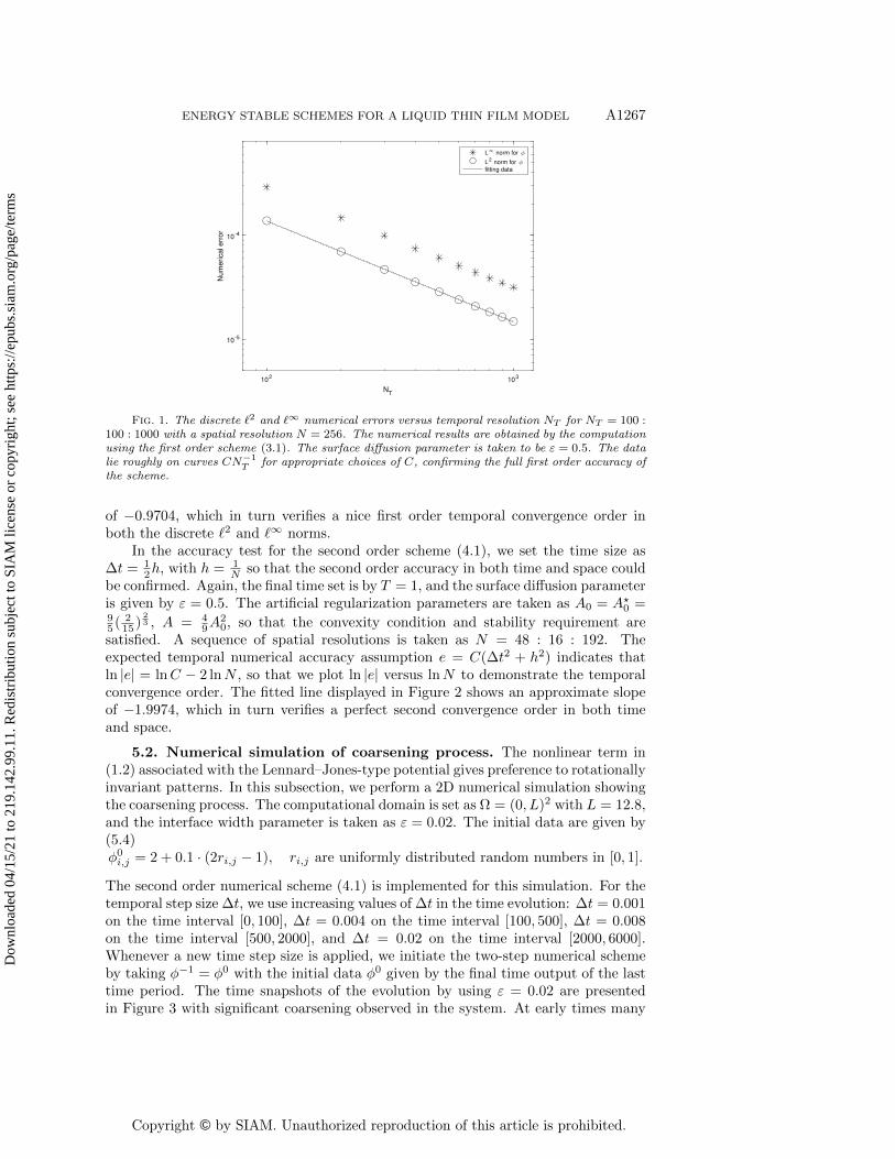
In the accuracy check for the first order scheme (3.1), we fix the spatial resolutionas N = 256 (with h = 1

256 ), so that the spatial numerical error is negligible. Thefinal time is set as T = 1, and the surface diffusion parameter is taken as \varepsilon = 0.5.Naturally, a sequence of time step sizes is taken as \Delta t = T

NTwith NT = 100 : 100 :

1000. The expected temporal numerical accuracy assumption e = C\Delta t indicates thatln | e| = ln(CT ) - lnNT , so that we plot ln | e| versus lnNT to demonstrate the temporalconvergence order. The fitted line displayed in Figure 1 shows an approximate slope

Dow

nloa

ded

04/1

5/21

to 2

19.1

42.9

9.11

. Red

istr

ibut

ion

subj

ect t

o SI

AM

lice

nse

or c

opyr

ight

; see

http

s://e

pubs

.sia

m.o

rg/p

age/

term

s



102

103

NT

10-5

10-4

Nu

me

rica

l err

or

L norm for

L2 norm for

fitting data

Fig. 1. The discrete \ell 2 and \ell \infty numerical errors versus temporal resolution NT for NT = 100 :100 : 1000 with a spatial resolution N = 256. The numerical results are obtained by the computationusing the first order scheme (3.1). The surface diffusion parameter is taken to be \varepsilon = 0.5. The datalie roughly on curves CN - 1

T for appropriate choices of C, confirming the full first order accuracy ofthe scheme.

of - 0.9704, which in turn verifies a nice first order temporal convergence order inboth the discrete \ell 2 and \ell \infty norms.

In the accuracy test for the second order scheme (4.1), we set the time size as\Delta t = 1

2h, with h = 1N so that the second order accuracy in both time and space could

be confirmed. Again, the final time set is by T = 1, and the surface diffusion parameteris given by \varepsilon = 0.5. The artificial regularization parameters are taken as A0 = A \star

0 =95 (

215 )

23 , A = 4

9A20, so that the convexity condition and stability requirement are

satisfied. A sequence of spatial resolutions is taken as N = 48 : 16 : 192. Theexpected temporal numerical accuracy assumption e = C(\Delta t2 + h2) indicates thatln | e| = lnC - 2 lnN , so that we plot ln | e| versus lnN to demonstrate the temporalconvergence order. The fitted line displayed in Figure 2 shows an approximate slopeof - 1.9974, which in turn verifies a perfect second convergence order in both timeand space.

5.2. Numerical simulation of coarsening process. The nonlinear term in(1.2) associated with the Lennard--Jones-type potential gives preference to rotationallyinvariant patterns. In this subsection, we perform a 2D numerical simulation showingthe coarsening process. The computational domain is set as \Omega = (0, L)2 with L = 12.8,and the interface width parameter is taken as \varepsilon = 0.02. The initial data are given by(5.4)\phi 0i,j = 2 + 0.1 \cdot (2ri,j - 1), ri,j are uniformly distributed random numbers in [0, 1].

The second order numerical scheme (4.1) is implemented for this simulation. For thetemporal step size \Delta t, we use increasing values of \Delta t in the time evolution: \Delta t = 0.001on the time interval [0, 100], \Delta t = 0.004 on the time interval [100, 500], \Delta t = 0.008on the time interval [500, 2000], and \Delta t = 0.02 on the time interval [2000, 6000].Whenever a new time step size is applied, we initiate the two-step numerical schemeby taking \phi - 1 = \phi 0 with the initial data \phi 0 given by the final time output of the lasttime period. The time snapshots of the evolution by using \varepsilon = 0.02 are presentedin Figure 3 with significant coarsening observed in the system. At early times many

Dow

nloa

ded

04/1

5/21

to 2

19.1

42.9

9.11

. Red

istr

ibut

ion

subj

ect t

o SI

AM

lice

nse

or c

opyr

ight

; see

http

s://e

pubs

.sia

m.o

rg/p

age/

term

s



40 60 80 100 120 140 160 180 200

N

10-6

10-5

10-4

Num

erica

l e

rro

r

L norm for

L2 norm for

fitting data

Fig. 2. The discrete \ell 2 and \ell \infty numerical errors versus spatial resolution N for N = 48 : 16 :192, and the time step size is set as \Delta t = 1

2h. The numerical results are obtained by the computation

using the second order scheme (4.1). The surface diffusion parameter is taken to be \varepsilon = 0.5. Thedata lie roughly on curves CN - 2 for appropriate choices of C, confirming the full second orderaccuracy of the scheme in both time and space.

small hills (yellow) are present with flat base (blue). At the final time, t = 6000, asingle hill structure emerges, and further coarsening is not possible.

The long time characteristics of the solution, especially the energy decay rate,are of interest to material scientists. Figure 4 presents the log-log plot for the energyversus time with the given physical parameters. Recall that, at the space-discretelevel, the energy, Fh is defined via (3.2). The detailed scaling ``exponent"" is obtainedusing least squares fits of the computed data up to time t = 100. A clear observa-tion of the aet

be scaling law can be made, with ae = 59.8167, be = - 0.1951. Forthe Cahn--Hilliard flow with polynomial approximation of the double-well energy po-tential, various numerical experiments have indicated an approximately t - 1/3 energydissipation law [9, 11]. For the droplet liquid film equation (1.2), with Lennard--Jones-type energy potential included in (1.1), this numerical evidence has implied adifferent energy dissipation scaling index with be = - 0.1951, in comparison with anapproximate t - 1/3 scaling law for the standard Cahn--Hilliard model.

Remark 5.2. The coarsening dynamics problem is usually a long time process.To improve the computational efficiency, some adaptive time stepping strategies havebeen extensively applied in such a long time simulation effort; our simulation hasalso used a variable time step size method as outlined above. There have been sometheoretical works for the time-adaptive methods in the computation of coarsening pro-cesses, such as those for the Cahn--Hilliard model [8] and epitaxial thin film model [40].The corresponding analysis for the time adaptive method applied to the droplet liquidfilm coarsening dynamics will be left to future works.

Remark 5.3. For the physical energy given by (1.1), the final steady state solutiondepends on \varepsilon and the the mass average of \phi , which is a conserved quantity. It is wellknown that if the mass average is less than or equal to 1, the steady state solutionturns out to be a trivial constant profile, due to its minimum energy constrained bythe mass average. On the other hand, if the mass average is greater than 1, the timecoarsening process and the final profile have interesting structures, as demonstrated

Dow

nloa

ded

04/1

5/21

to 2

19.1

42.9

9.11

. Red

istr

ibut

ion

subj

ect t

o SI

AM

lice

nse

or c

opyr

ight

; see

http

s://e

pubs

.sia

m.o

rg/p

age/

term

s



t = 6, 20 t = 40, 60

t = 100, 200 t = 300, 400

t = 500, 900 t = 2000, 6000

Fig. 3. Snapshots of the computed height function \phi at the indicated times for the parametersL = 12.8, \varepsilon = 0.02. Finally, there is a single droplet structure. (Figure in color online.)

100

101

102

103

101

Fig. 4. Log-log plot of the temporal evolution of the energy Fh for \varepsilon = 0.02. The energydecreases like aetbe until saturation. The red lines represent the energy plot obtained by the sim-ulations, while the straight lines are obtained by least squares approximations to the energy data.The least squares fit is only taken for the linear part of the calculated data only up to approximatelytime t = 100. The fitted line has the form aetbe with ae = 59.8167, be = - 0.1951. (Figure in coloronline.)

Dow

nloa

ded

04/1

5/21

to 2

19.1

42.9

9.11

. Red

istr

ibut

ion

subj

ect t

o SI

AM

lice

nse

or c

opyr

ight

; see

http

s://e

pubs

.sia

m.o

rg/p

age/

term

s



in our reported numerical results. Under circumstances when the initial data con-tain certain values near zero at a certain region, the singular and convex nature ofthe Lennard--Jones-type energy potential (1.1) will push the solution away from thesingular value of 0; in this case, if the mass average is greater than 1, one could stillobserve an interesting coarsening process, similar to our numerical simulation result.

6. Concluding remarks. Two finite difference numerical schemes, includingboth the first and second order accurate algorithms, are proposed and analyzed forthe droplet liquid film model in which a singular Lennard--Jones energy potential isinvolved. In the first order scheme, the convex potential and the surface diffusionterms are updated implicitly, while the concave potential term is updated explicitly.A theoretical justification of the unique solvability and positivity-preserving propertyis provided, so that a singularity is avoided in the scheme. Such an analysis is based onthe subtle fact that the numerical solution is equivalent to a minimization of a convexnumerical energy, and the singular nature of the Lennard--Jones potential term aroundthe value of 0 prevents the numerical solution reaching such a singular value. The en-ergy stability of the numerical schemes comes from the convex-concave decompositionof the physical energy. In the second order scheme, an alternate convex-concave de-composition is formulated so that the concave part corresponds to a quadratic energy.In turn, the BDF temporal stencil is applied, the combined Lennard--Jones potentialterm is treated implicitly, the concave expansive part is approximated by a secondorder Adams--Bashforth explicit extrapolation, and an artificial Douglas--Dupont reg-ularization term is added to ensure the energy stability. The unique solvability andthe positivity-preserving property for the second order scheme could be similarly es-tablished, in which the convexity of the \phi - 8 term has played an important role. Thepreconditioned steepest descent iteration solver has been applied to implement thenonlinear numerical schemes due to the fact that the implicit part turns out to bethe gradient of a strictly convex energy functional. A few numerical results are alsopresented in this paper which demonstrate the robustness of the proposed numericalscheme.

REFERENCES

[1] O. Alexander and S.G. Bankoff, Dewetting of a heated surface by an evaporating liquid filmunder conjoining/disjoining pressures, J. Colloid Interface Sci., 218 (1999), pp. 152--166.

[2] O. Alexander, S.H. Davis, and S.G. Bankoff, Long-scale evolution of thin liquid films, Rev.Mod. Phys., 69 (1997), pp. 931--980.

[3] K.S. Anna, Z.Y. Zhang, and J.F. Wendelken, Island diffusion and coarsening on metal(100) surfaces, Phys. Rev. Lett., 79 (1997), pp. 3210--3213.

[4] J. Becker, G. Grun, R. Seeman, H. Mantz, K. Jacobs, K.R. Mecke, and R. Blossey,Complex dewetting scenarios captured by thin-film models, Nat. Mater., 2 (2003), pp. 59--63.

[5] A.L. Bertozzi, G. Grun, and T.P. Witelski, Dewetting films: Bifurcations and concentra-tions, Nonlinearity, 14 (2001), pp. 1569--1592.

[6] W. Chen, C. Wang, S. Wang, X. Wang, and S. Wise, Energy stable numerical schemes fora ternary Cahn-Hilliard system, J. Sci. Comput., 84 (2020), 27.

[7] W. Chen, C. Wang, X. Wang, and S.M. Wise, Positivity-preserving, energy stable numericalschemes for the Cahn-Hilliard equation with logarithmic potential, J. Comput. Phys.: X,3 (2019), 100031.

[8] W. Chen, X. Wang, Y. Yan, and Z. Zhang, A second order bdf numerical scheme withvariable steps for the Cahn-Hilliard equation, SIAM J. Numer. Anal., 57 (2019), pp. 495--525, https://doi.org/10.1137/18M1206084.

[9] K. Cheng, W. Feng, C. Wang, and S.M. Wise, An energy stable fourth order finite differencescheme for the Cahn-Hilliard equation, J. Comput. Appl. Math., 362 (2019), pp. 574--595.

Dow

nloa

ded

04/1

5/21

to 2

19.1

42.9

9.11

. Red

istr

ibut

ion

subj

ect t

o SI

AM

lice

nse

or c

opyr

ight

; see

http

s://e

pubs

.sia

m.o

rg/p

age/

term

s

https://doi.org/10.1137/18M1206084



[10] K. Cheng, C. Wang, and S.M. Wise, An energy stable Fourier pseudo-spectral numericalscheme for the square phase field crystal equation, Commun. Comput. Phys., 26 (2019),pp. 1335--1364.

[11] K. Cheng, C. Wang, S.M. Wise, and X. Yue, A second-order, weakly energy-stable pseudo-spectral scheme for the Cahn-Hilliard equation and its solution by the homogeneous lineariteration method, J. Sci. Comput., 69 (2016), pp. 1083--1114.

[12] L. Cherfils, A. Miranville, and S. Zelik, The Cahn-Hilliard equation with logarithmicpotentials, Milan J. Math., 79 (2011), pp. 561--596.

[13] L. Dong, C. Wang, H. Zhang, and Z. Zhang, A positivity-preserving, energy stable and con-vergent numerical scheme for the Cahn-Hilliard equation with a Flory-Huggins-deGennesenergy, Commun. Math. Sci., 17 (2019), pp. 921--939.

[14] L. Dong, C. Wang, H. Zhang, and Z. Zhang, A positivity-preserving second-order BDFscheme for the Cahn-Hilliard equation with variable interfacial parameters, Commun.Comput. Phys., 28 (2020), pp. 967--998.

[15] Q. Du, L. Ju, X. Li, and Z. Qiao, Maximum principle preserving exponential time differencingschemes for the nonlocal Allen-Cahn equation, SIAM J. Numer. Anal., 57 (2019), pp. 875--898, https://doi.org/10.1137/18M118236X.

[16] Q. Du, L. Ju, X. Li, and Z. Qiao, Maximum bound principles for a class of semi-linearparabolic equations and exponential time differencing schemes, SIAM Rev., accepted andin press, https://arxiv.org/abs/2005.11465.

[17] W. Feng, Z. Guan, J.S. Lowengrub, C. Wang, S.M. Wise, and Y. Chen, A uniquelysolvable, energy stable numerical scheme for the functionalized Cahn-Hilliard equationand its convergence analysis, J. Sci. Comput., 76 (2018), pp. 1938--1967.

[18] W. Feng, A.J. Salgado, C. Wang, and S.M. Wise, Preconditioned steepest descent methodsfor some nonlinear elliptic equations involving p-Laplacian terms, J. Comput. Phys., 334(2017), pp. 45--67.

[19] W. Feng, C. Wang, S.M. Wise, and Z. Zhang, A second-order energy stable backward differ-entiation formula method for the epitaxial thin film equation with slope selection, Numer.Methods Partial Differ. Equ., 34 (2018), pp. 1975--2007.

[20] A. Giorgini, M. Grasselli, and A. Miranville, The Cahn-Hiliard-Oono equation with sin-gular potential, Math. Models Methods Appl. Sci., 27 (2017), pp. 2485--2510.

[21] K.B. Glasner, Ostwald ripening in thin film equations, SIAM J. Appl. Math., 69 (2008),pp. 473--493, https://doi.org/10.1137/080713732.

[22] K.B. Glasner and T.P. Witelski, Coarsening dynamics of dewetting films, Phys. Rev. E.,67 (2003), 016302.

[23] J. Guo, C. Wang, S.M. Wise, and X. Yue, An H2 convergence of a second-order convex-splitting, finite difference scheme for the three-dimensional Cahn-Hilliard equation, Com-mun. Math. Sci., 14 (2016), pp. 489--515.

[24] Y. Hao, Q. Huang, and C. Wang, A third order BDF energy stable linear scheme for theno-slope-selection thin film model, Commun. Comput. Phys., 29 (2021), pp. 905--929.

[25] J.N. Israelachvili, Intermolecular and Surface Forces, Academic Press, New York, 1992.[26] J. Kim, Numerical simulations of phase separation dynamics in a water-oil-surfactant system,

J. Colloid Interface Sci., 303 (2006), pp. 272--279.[27] R.V. Kohn and F. Otto, Upper bound on coarsening rate, Commun. Math. Phys., 229 (2002),

pp. 375--395.[28] R.V. Kohn and X.D. Yan, Coarsening rates for models of multicomponent phase separation,

Interface Free Bound., 6 (2004), pp. 135--149.[29] D. Li and Z. Qiao, On second order semi-implicit Fourier spectral methods for 2D Cahn-

Hilliard equations, J. Sci. Comput., 70 (2017), pp. 301--341.[30] D. Li and Z. Qiao, On the stabilization size of semi-implicit Fourier-spectral methods for 3D

Cahn-Hilliard equations, Commun. Math. Sci., 15 (2017), pp. 1489--1506.[31] W. Li, W. Chen, C. Wang, Y. Yan, and R. He, A second order energy stable linear scheme

for a thin film model without slope selection, J. Sci. Comput., 76 (2018), pp. 1905--1937.[32] R. Limary and P.F. Green, Late-stage coarsening of an unstable structured liquid film, Phys.

Rev. E., 66 (2002), 021601.[33] R. Limary and P.F. Green, Dynamics of droplets on the surface of a structured fluid film:

Late-stage coarsening, Langmuir, 19 (2003), pp. 2419--2424.[34] X. Meng, Z. Qiao, C. Wang, and Z. Zhang, Artificial regularization parameter analysis

for the no-slope-selection epitaxial thin film model, CSIAM Trans. Appl. Math., 1 (2020),pp. 441--462.

[35] A. Miranville, On a phase-field model with a logarithmic nonlinearity, Appl. Math., 57 (2012),pp. 215--229.

Dow

nloa

ded

04/1

5/21

to 2

19.1

42.9

9.11

. Red

istr

ibut

ion

subj

ect t

o SI

AM

lice

nse

or c

opyr

ight

; see

http

s://e

pubs

.sia

m.o

rg/p

age/

term

s

https://doi.org/10.1137/18M118236X

https://arxiv.org/abs/2005.11465

https://doi.org/10.1137/080713732



[36] A. Oron, S.H. Davis, and S.G. Bankoff, Long-scale evolution of thin liquid films, Rev. Mod.Phys., 69 (1997), pp. 932--977.

[37] F. Otto, T. Rump, and D. Slepcev, Coarsening rates for a droplet model: Rigorous upperbounds, SIAM J. Math. Anal., 38 (2006), pp. 503--529, https://doi.org/10.1137/050630192.

[38] R.L. Pbgo and A.M. Stuart, Front migration in the nonlinear Cahn-Hilliard equation, Proc.R. Soc. Lond., 422 (1989), pp. 261--278.

[39] L.M. Pismen, Spinodal dewetting in a volatile liquid film, Phys. Rev. E., 70 (2004), 021601.[40] Z. Qiao, Z. Zhang, and T. Tang, An adaptive time-stepping strategy for the molecular beam

epitaxy models, SIAM J. Sci. Comput., 33 (2011), pp. 1395--1414, https://doi.org/10.1137/100812781.

[41] S. Ravati and B.D. Favis, Interfacial coarsening of ternary polymer blends with partial andcomplete wetting structures, Polymer, 54 (2013), pp. 6739--6751.

[42] U. Thiele, M.G. Velarde, and K. NeuKer, Dewetting: Film rupture by nucleation in thespinodal regime, Phys. Rev. Lett., 87 (2001), 016104.

[43] C. Wang and S.M. Wise, An energy stable and convergent finite-difference scheme for themodified phase field crystal equation, SIAM J. Numer. Anal., 49 (2011), pp. 945--969,https://doi.org/10.1137/090752675.

[44] S.M. Wise, Unconditionally stable finite difference, nonlinear multigrid simulation of theCahn-Hilliard-Hele-Shaw system of equations, J. Sci. Comput., 44 (2010), pp. 38--68.

[45] S.M. Wise, C. Wang, and J. Lowengrub, An energy stable and convergent finite-differencescheme for the phase field crystal equation, SIAM J. Numer. Anal., 47 (2009), pp. 2269--2288, https://doi.org/10.1137/080738143.

[46] Y. Yan, W. Chen, C. Wang, and S.M. Wise, A second-order energy stable BDF numericalscheme for the Cahn-Hilliard equation, Commun. Comput. Phys., 23 (2018), pp. 572--602.

Dow

nloa

ded

04/1

5/21

to 2

19.1

42.9

9.11

. Red

istr

ibut

ion

subj

ect t

o SI

AM

lice

nse

or c

opyr

ight

; see

http

s://e

pubs

.sia

m.o

rg/p

age/

term

s

https://doi.org/10.1137/050630192

https://doi.org/10.1137/100812781

https://doi.org/10.1137/100812781

https://doi.org/10.1137/090752675

https://doi.org/10.1137/080738143

structure-preserving, energy stable numerical schemes for

Documents