structure preserving model order reduction via krylov subspace projection · structure preserving...
TRANSCRIPT

Structure Preserving Model Order Reduction
via Krylov Subspace Projection
Zhaojun BaiUniversity of California, Davis
http://www.cs.ucdavis.edu/∼bai
COMSON Autumn School on Future Developments in Model Order ReductionTerschelling, The Netherlands, Sep. 21-25, 2009

Outline
A. A unified theory for SPMOR
B. Case study: RCL/RCS circuits
C. Open problems and future development
D. Work in progress: SPMOR with optimal moment-matching

Outline
A. A unified theory for SPMOR
joint with R. C. Li of Univ. of Texas, Arlington
B. Case study: RCL/RCS circuits
mostly due to Y. Su and X. Zeng group at Fudan Univ., China
C. Open problems and future development
D. Work in progress: SPMOR with optimal moment-matching
joint with Y.Li and W.-W. Lin of National Chiao Tung Univ., Taiwan

Outline of Part A – a unified SPMOR theory
1. Transfer function in the first-order form
2. Model order reduction
3. The moment-matching theorem
4. SPMOR
(a) Basic formulation
(b) A generic algorithm
(c) Structure of Krylov subspace
(d) Structured Arnoldi procedure (framework)
joint with R. C. Li of Univ. of Texas, Arlington

Transfer function in the first-order form A.1
• Consider the matrix-valued transfer function of the first-order multi-inputmulti-output (MIMO) linear dynamical system
H(s) = LT(sC + G)−1B,
where C and G are N ×N , B is N ×m and L is N × p.
• Assume that G is nonsingular.
• The transfer function can be expanded around s = 0 as
H(s) =
∞∑�=0
(−1)�s�LT(G−1C)�G−1B
≡∞∑�=0
(−1)�s�M�,
whereM� = LT(G−1C)�G−1B
are referred to as the moments at s = 0.

• In the case when G is singular or approximations to H(s) around a selectedpoint s0 �= 0 are sought, a shift
s = (s− s0) + s0 ≡ σ + s0
can be performed and then
sC + G = (s− s0)C + s0C + G ≡ σC + (s0C + G).
Upon substitutions (i.e., renaming)
G← s0C + G, s← σ,
the problem of approximating H(s) around s = s0 becomes equivalent toapproximate the substituted H(σ) around σ = 0.
• Many transfer functions appearing in different forms can be re-formulated inthe first order form.

Example: RCL circuits
• The MNA formulation of RCL circuits in the Integro-DAEs form:⎧⎨⎩ C ddtz(t) + Gz(t) + Γ
∫ t
0
z(τ )dτ = Bu(t),
y(t) = BTz(τ ).
• The transfer function of the Integro-DAEs is given by
H(s) = BT
(sC + G +
1
sΓ
)−1
B.
• References: [Freund], [Gad et al] in [S-vdV-R]

• Linearization #1:
Define
C =
[C 00 −W
], G =
[G ΓW 0
], L = B =
[B0
]for any nonsingular matrix W .Then the transfer function:
H(s) = BT(sC + G)−1B.
• Linearization #2:
Define
C =
[G CW 0
], G =
[Γ 00 −W
], L = B =
[B0
]for any nonsingular matrix W
Then the transfer function:
H(s) = sBT(sC + G)−1B.

• Remarks:
1. In the linearization #2, the matrix-vector products with the matrices G−1Cand G−TCT are much easier to do than the linearization #1.
2. The linearization #1 favors approximations around s =∞.
3. In the case when approximations near a finite point s0 �= 0 are sought, ashift must be performed and then neither linearization has cost advantageover the other because the s0C + G is no longer block diagonal.
4. If the shift is performed before linearization, the same advantage as thelinearization #2 over the linearization #1 for approximations near s = 0 isretained.

Example: Coupled systems
• The transfer function of interconnected (coupled) systems:
H(s) = LT0 (I −W (s)E)−1 W (s)B0,
where E is the subsystem incidence matrix for connecting subsystemsH1(s), . . . , Hk(s), and
W (s) = diag( H1(s), . . . , Hk(s) )
= diag( LT1(sI − A1)
−1B1, . . . , LTk(sI − Ak)
−1Bk ).
• Let
A = diag(A1, . . . , Ak), B = diag(B1, . . . , Bk), L = diag(L1, . . . , Lk),
Then H(s) can be turned into the first-order form
H(s) = LT(sC + G)−1B,
whereC = I, G = −A−BEL, B = BB0 L = LL0.
• References: [Reis and Stykel] and [Vandendorpe and van Dooren] in[S-vdV-R]

Model order reduction A.2
• Model order reduction of the transfer function H(s) via subspace projectionstarts by computing matrices
X ,Y ∈ RN×n such that YTGX is nonsingular,
• Then defines a reduced-order transfer function
Hr(s) = LTr (sCr + Gr)
−1Br,
where
Cr = YTCX , Gr = YTGX , Br = YTB, Lr = X TL. (1)
• The reduced transfer function H r(s) can be expanded around s = 0:
Hr(s) =∞∑�=0
(−1)�s�LTr (G−1
r Cr)�G−1
r Br =∞∑�=0
(−1)�s�Mr,�,
whereMr,� = LT
r (G−1r Cr)
�G−1r Br
are referred to as the moments of the reduced system.

• Desired properties:
1. n� N .
2. By choosing X and Y right, the reduced system associated with the reducedtransfer function can be made to resemble the original system enough tohave practical relevance: Moment matching, stability, passivity, ...

Krylov subspaces associated with H(s)
• Transfer function
H(s) = LT(sC + G)−1B = LT(sG−1C + I)−1G−1B
• Two associated Krylov subspace
1. Right Krylov subspace:
Kk(G−1C,G−1B) =
span{G−1B, (G−1C)G−1B, (G−1C)2G−1B, . . . (G−1C)k−1G−1B, }2. Left Krylov subspace:
Kk(G−TCT,G−TL) =
span{G−TL, (G−TCT)G−TL, (G−TCT)2G−TL, . . . (G−TCT)k−1G−TL, }• Numerical stable computation of the bases of these Krylov subspaces are
nontrivial tasks – Gutknecht’s talk

The moment-matching theorem A.3
The following theorem dictates how good a reduced transfer function Hr(s)approximates the original transfer function H(s).
Theorem. Suppose that G and Gr are nonsingular. If
Kk(G−1C,G−1B) ⊆ span{X}
andKj(G
−TCT,G−TL) ⊆ span{Y},then the moments of H(s) and of its reduced function Hr(s) satisfy
M� = Mr,� for 0 ≤ � ≤ k + j − 1,
which implyHr(s) = H(s) +O(sk+j).

Remarks:
• The conditions suggest that by enforcing span{X} and/or span{Y} to containmore appropriate Krylov subspaces associated with multiple points, Hr(s) canbe made to approximate H(s) well near all those points – multi-pointapproximation.
• When G = I, it is due to [Villemagne and Skelton’87]
• The general form as stated above was proved by [Grimme’97]
• A different proof is available in [Freund’05]
• A proof using the projection language was given in [Li and B.’05].
• Its implication to structure-preserving model reduction was also realized in [Liand B.’05] and [Freund’05]

Structure-preserving model order reduction (SPMOR) A.4
• System structure:
For the simplicity of exposition, consider system matrices G, C, B, and Lhaving the following 2× 2 block structure
C =
[ N1 N2
N ′1 C11 0N ′2 0 C22
], G =
[ N1 N2
N ′1 G11 G12
N ′2 G21 0
],
B =
[ p
N ′1 B1
N ′2 0
], L =
[ m
N1 L1
N2 0
],
(2)
where N1 + N2 = N ′1 + N ′2 = N .
System matrices from the time-domain modified nodal analysis (MNA) circuitequations of RCL circuits take such forms. (more later)

• The objectives of SPMOR:
1. structurally preserves the block structure:
Cr =
[ n1 n2
n′1 Cr,11 0n′2 0 Cr,22
], Gr =
[ n1 n2
n′1 Gr,11 Gr,12
n′2 Gr,21 0
],
Br =
[ p
n′1 Br,1
n′2 0
], Lr =
[ m
n1 Lr,1
n2 0
],
(3)
where n1 + n2 = n′1 + n′2 = n.
2. Each sub-block is a direct reduction from the corresponding sub-block inthe original system.
• Advantages of SPMOR:
1. Easily provable preservation of the original system properties, such asstability, passivity, ...
2. Better numerical stability and accuracy
3. ...

Basic formulation A.4.a
In the formulation of subspace projection, SPMOR objectives can beaccomplished by picking the projection matrices
X =
[ n1 n2
N1 X1
N2 X2
], Y =
[ n′1 n′2N ′1 Y1
N ′2 Y2
].
Then
YTCX =
[Y T
1
Y T2
] [C11 00 C22
] [X1
X2
]=
[Cr,11 0
0 Cr,22
]= Cr,
YTGX =
[Y T
1
Y T2
] [G11 G12
G21 0
] [X1
X2
]=
[Gr,11 Gr,12
Gr,21 0
]= Gr,
YTB =
[Y T
1
Y T2
] [B1
0
]=
[Br,1
0
]= Br,
X TL =
[XT
1
XT2
] [L1
0
]=
[Lr,1
0
]= Lr.
For the case when Y is taken to be the same as X , this idea is exactly the so-called“split congruence transformations” [Kerns and Yang’97].

A generic algorithm A.4.b
A generic algorithm to generate the desired projection matrices X and Y:
• Compute the basis matrices X and Y such that
Kk(G−1C,G−1B) ⊆ span
{X}
andKj(G
−TCT,G−TL) ⊆ span{
Y}
.
• Partition X and Y as
X =
[X1
X2
]and Y =
[Y1
Y2
]consistently with the block structures in G, C, L, and B, and then perform
X =
[X1
X2
]� X =
[X1
X2
]and Y =
[Y1
Y2
]� Y =
[Y1
Y2
].
satisfying
span{
X}⊆ span {X} and span
{Y}⊆ span {Y} (4)

Remarks
• The subspace embedding task “�” can be accomplished as follows:
1. Compute Zi having full column rank such that span{Zi} ⊆ span{Zi};2. Output Z =
[Z1
Z2
].
• There are a variety of ways to realize Step 1: Rank revealing QRdecompositions, modified Gram-Schmidt process, or SVD.
• For maximum efficiency, one should make Zi have as fewer columns as onecan. Notice the smallest possible number is rank(Zi), but one may have to adda few extra columns to make sure the total number of columns in all Xi andthat in all Yi are the same when constructing X and Y .
• There are numerically more efficient alternatives when further characteristicsin the sub-blocks in G and C is known – (more later)
• The first k + j moments of H(s) and the SPMOR transfer function Hr(s)match.
Proof: a direct consequence of the moment-matching theorem and the genericalgorithm.

Structure of Krylov subspace A.4.c
The first-computing-then-splitting can be combined into one to generate thedesired X and Y directly, by taking advantage of a structural property of Krylovsubspaces for certain block matrix.
Theorem. Suppose that A and B admit the following partitioning
A =
[ N N
N A11 A12
N αI 0
], B =
[ p
N B1
N B2
],
where α is a scalar. Let a basis matrix X of the Krylov subspace Kk(A,B)be partitioned as
X =
[N X1
N X2
].
Thenspan{X2} ⊆ span{B2, X1}.

Remarks:
1. This theorem provides a theoretical foundation to simply compute X1, thenexpand X1 to X1 so that span{X1} = span{B2, X1} and finally set
X =
[X1
X1
].
2. The theorem was implicitly implied in [Su and Craig’91, Bai and Su’05] andexplicitly stated in [Li and Bai’05] for more general cases.

Structured Arnoldi procedure A.4.d
• For A =
[A11 A12
αI
], X1 can be computed directly by the following structured
Arnoldi procedure.
• A simple-minded version for illustrating the key ingredients. Practicalimplementation will have to incorporate the possibility when various QRdecompositions produce (nearly) singular upper triangular matrices R.
• The second-order Arnoldi process (SOAR) is an implementation of suchstructured Arnoldi process.

Structured Arnoldi process (framework)
1. B1 = Q1R (QR decomposition)2. P1 = αB2R
−12
3. for j = 1, 2, . . . , k do4. T = A11Qj + A12Pj
5. S = αQj
6. for i = 1, 2, . . . , j do7. Z = QT
i T
8. T = T −QiZ
9. S = S − PiZ
10. enddo11. T = QjR (QR decomposition)12. Pj = SR−1
13. enddo14. X1 = [Q1, Q2, . . . , Qk]
15. T = B2;16. for j = 1, 2, . . . , k do17. Z = QT
j T
18. T = T −QjZ
19. enddo20. T = QR (QR decomposition)21. X1 = [X1, Q]

FE Model
No. of element : 22,884No. of node : 28,752No. of constraint : 96No. of DoF : 86,160
COMBIN14: stiffness + damping
observationpoint

10-910-810-710-610-5
101 102 103 104-180-90
090
180
ANSYS (FM)
Ampl
itude
[µm
]
y-direction
Phas
e [de
gree
]
Frequency [Hz]
Harmonic Analysis: Full Method
50 hr

Harmonic Analysis: MOR (SOAR)
10-910-810-710-610-5
101 102 103 104-180-90
090
180
MOR (n=100)
Ampl
itude
[µm
]
y-direction
Phas
e [de
gree
]
Frequency [Hz]
1,500 sec

Harmonic Analysis:Mode Superposition Method
8,000 sec
10-910-810-710-610-5
101 102 103 104-180-90
090
180
MS (m=100)
Ampl
itude
[µm
]
y-direction
Phas
e [de
gree
]
Frequency [Hz]

Harmonic Analysis: Reduced Method
4,500 sec
10-910-810-710-610-5
101 102 103 104-180-90
090
180
RM (n=100)
Ampl
itude
[µm
]
y-direction
Phas
e [de
gree
]
Frequency [Hz]

Outline of Part B – Case study: RCL circuits
• RCL and RCS circuit equations
• Transfer functions
• SPMOR – version 1
• Towards a synthesizable reduced-order RCL system
– Expanded RCL (RCS) equations
– Transfer function
– SPMOR – version 2
– Preserving I/O ports
– Diagonalization
– Reduced-order RCL equation – synthesizable yet?
– An example
mostly due to Y. Su and X. Zeng group at Fudan Univ., China

RCL circuit equations B.1
The MNA (modified nodal analysis) formulation of an RCL circuit network infrequency domain is of the form⎧⎪⎪⎨⎪⎪⎩
(s
[C 00 L
]+
[G E−ET 0
])[v(s)i(s)
]=
[Bv
0
]u(s),
y(s) =[DT
v 0] [ v(s)
i(s)
],
(5)
where
• v(s) and i(s) denote N1 nodal voltage and N2 auxiliary branch currents;
• u and y are the input current sources and output voltages;
• Bv and Dv denote the incidence matrices for the input current sources andoutput node voltages;
• C,L and G represent the contributions of the capacitors, inductors andresistors; and
• E is the incidence matrix for the inductances.

RCS circuit equations
• When an RCL network is modeled with a 3-D extraction method forinterconnection analysis, the resulted inductance matrix L is usually very largeand dense.
• As an alternative approach, we can use the susceptance matrix S = L−1, whichis sparse after dropping small entries:
• RCS circuit equations:⎧⎪⎪⎨⎪⎪⎩(
s
[C 00 I
]+
[G E−SET 0
])[v(s)i(s)
]=
[Bv
0
]u(s),
y(s) =[DT
v 0] [ v(s)
i(s)
].

RCL/RCS transfer function B.2
• Eliminating the branch current variable i(s) of the RCL and RCS equations, wehave the second-order form{ (
sC + G + 1sΓ)
v(s) = Bvu(s),
y(s) = DTv v(s),
whereΓ = EL−1ET = ESET.
• The transfer function H(s):
H(s) = DTv
(sC + G +
1
sΓ
)−1
Bv.
• Perform the shift “s→ s0 + σ” to get
H(s) = sDTv (s2C + sG + Γ)−1Bv
= (s0 + σ) DTv [σ2C + σ(2s0C + G) + (s2
0C + s0G + Γ)]−1Bv
= (s0 + σ)LT(σC + G)−1B,

where
C =
[G0 CW 0
], G =
[Γ0 00 −W
], L =
[Dv
0
], B =
[Bv
0
], (6)
and G0 = 2s0C + G, Γ0 = s20C + s0G + Γ and W is any nonsingular matrix.

SPMOR – version 1 B.3
• The SPRIM method [Freund’04] provides a SPMOR model for the RCLequations.
• The following is an alternative SPMOR model, referred to as the SAPORmethod [Yang et al’04].
• For the system matrices C, G and B,
G−1C =
[Γ−1
0 G0 Γ−10 C
−I 0
], G−1B =
[Γ−1
0 Bv
0
].
• By using the block structure of G, and applying the SOAR, we can generate Xr
with orthonormal columns such that
Kk(G−1C,G−1B) ⊆ span
{[Xr
Xr
]}• The subspace projection technique can be viewed as a change-of-variable:
v(s) ≈ Xrvr(s),
where vr(s) is a vector of dimension n.

• Substituting into the RCS equation, yields⎧⎨⎩(
sCr + Gr +1
sΓr
)vr(s) = Br,vu(s),
y(s) = DTr,vvr(s),
whereCr = XT
r CXr, Gr = XTr GXr, Γr = ET
r ΓEr, Er = XTr E,
andBr,v = XT
r Bv, Dr,v = XTr Dv.
• The transfer function of the reduced system is given by
Hr(s) = DTr,v
(sCr + Gr +
1
sΓr
)−1
Br,v.

• By setting
X = Y =
[ n N2
N1 Xr
N2 I
],
The reduced second-order form corresponds to a reduced order SAPOR systemof the original RCS equations:⎧⎪⎪⎨⎪⎪⎩
(s
[Cr 00 I
]+
[Gr Er
−SETr 0
])[vr(s)i(s)
]=
[Br,v
0
]u(s),
y(s) =[DT
r,v 0] [ vr(s)
i(s)
].
Note that i(s) is a vector of N2 components, the same as the original auxiliarybranch currents i(s).

Towards a synthesizable reduced-order RCL system B.4
• The SAPOR system preserves the block structures and the symmetry of systemdata matrices of the original RCS system.
• However, the matrix Er in the SAPOR cannot be interpreted as an incidencematrix.
• Towards the objective of synthesis based on the reduced-order model, we shallreformulate the projection and the SAPOR system [Yang et al’08]

Expanded RCL/RCS equation B.4.a
• Leti(s) = E i(s).
Then the original RCS equations can be written as as an expanded RCS (RCSe)equations:⎧⎪⎪⎨⎪⎪⎩
(s
[C 00 I
]+
[G I−Γ 0
])[v(s)
i(s)
]=
[Bv
0
]u(s),
y(s) =[DT
v 0] [ v(s)
i(s)
].
• Note that the incidence matrix E in the original RCS equations is now theidentity matrix I .
• The new current vector i(s) is of the size N1, typically N1 ≥ N2. The order ofRCSe equations is 2N1.

RCSe transfer function B.4.b
In the first-order form, the transfer function H(s) of the RCSe equations:
H(s) = LT(sC + G)−1B,
where G and C are 2N1 × 2N1:
C =
[C 00 I
], G =
[G I−Γ 0
],
and
B =
[Bv
0
], L =
[Dv
0
].

SPMOR – version 2 B.4.c
Let
X = Y =
[ n n
N1 Xr
N1 Xr
].
Then by the change-of-variables
v(s) ≈ XTr vr(s) and i(s) ≈ XT
r ir(s),
and using the projection procedure, we have the reduced-order RCSe equations⎧⎪⎪⎨⎪⎪⎩(
s
[Cr 00 I
]+
[Gr I−Γr 0
])[vr(s)ir(s)
]=
[Br,v
0
]u(s),
y(s) =[DT
r,v 0] [ vr(s)
ir(s)
].
Note that the reduced equations not only preserve the 2-by-2 block structure of thesystem data matrices G and C, but also preserve the identity of the incidencematrix.

Preserving I/O port B.4.d
• For the objective of synthesis, let us further consider the structures of the inputand output matrices and the incidence matrix.
• Assume that the sub-blocks Bv and Dv in the input and output of the RCSequations are of the forms:
Bv =
[ p
p1 Bv1
N1−p1 0
], Dv =
[ m
p1 Dv1
N1−p1 0
].
• Furthermore, assume that the incidence matrix E has the zero block on the top,conformal with the partition of the input and output matrices:
E =
[ N2
p1 0
N1−p1 E
].
This assumption means that there is no susceptance (inductor) directlyconnecting to the input and output nodes.

• let Xr be an orthonormal basis for the projection subspace Usingpartitioning-and-embedding steps, we have
Xr =
[ n
p1 X(1)r
N1−p1 X(2)r
]� Xr =
[ p1 n
p1 IN1−p1 X2
],
where the columns of X2 form an orthonormal basis for the range of X(2)r . For
simplicity, we assume that there is no deflation, namely,rank(X
(2)r ) = rank(X2) = n.
Using the subspace projection with
X = Y =
[ p1+n p1+n
N1 Xr
N1 Xr
],
we have the reduced-order RCSe equations⎧⎪⎪⎨⎪⎪⎩(
s
[Cr 00 I
]+
[Gr I−Γr 0
])[vr(s)ir(s)
]=
[Br,v
0
]u(s),
y(s) =[DT
r,v 0] [ vr(s)
ir(s)
],

where Cr, Gr and Γr are (p1 + n)× (p1 + n) matrices:
Cr = XTr CXr, Gr = XT
r GXr, Γr = XTr ΓXr,
and the input and output sub-block matrices Br,v and Dr,v preserve the originalI/O structure:
Br,v = XTr
[Bv1
0
]=
[ p
p1 Bv1
n 0
], Dr,v = XT
r
[Dv1
0
]=
[ m
p1 Dv1
n 0
].
Note that
span
{[Xr
Xr
]}⊆ span
{[Xr
Xr
]}.
• The reduced RCSe system also preserves the same moment-matching property.

Diagonalization B.4.e
• Again for objective of synthesis, let us turn to the diagonalization of Γ in theRCSe equations:
• The “zero-block” assumption of the incidence matrix E implies that Γ is of theform
Γ = EL−1ET =
[ p1 N1−p1
p1 0 0
N1−p1 0 Γ
].
• It can be seen that in the reduced RCSe equations Γr has the same form
Γr =
[ p1 n
p1 0 0
n 0 Γr
],
where Γr = QT2 ΓQ2.
• Note that Γ is symmetric semi-positive definite, so is Γr.

• LetΓr = V ΛV T
be the eigen-decomposition of Γr, where V is orthogonal and Λ is diagonal.
• Define
V =
[ p1+n p1+n
p1+n V
p1+n V
],
where
V =
[ p1 n
p1 I
n V
].
• Then by a congruence transformation using the matrix V , the reduced-orderRCSe equations is equivalent to the equations⎧⎪⎪⎪⎨⎪⎪⎪⎩
(s
[Cr 00 I
]+
[Gr I
−Γr 0
])[vr(s)
ir(s)
]=
[Br,v
0
]u(s),
y(s) =[
DTr,v 0
] [ vr(s)
ir(s)
],

where vr(s) = V Tvr(s) and ir(s) = V Tir(s). Cr, Gr and Γr are(p1 + n)× (p1 + n) matrices:
Cr = V TCrV , Gr = V TGrV , Γr = V TΓrV .
Moreover with V being block diagonal, the input and output structures arepreserved, too:
Br,v = V TBr,v =
[ p
p1 Bv1
n 0
], Dr,v = V TDr,v =
[ p
p1 Dv1
n 0
].
• We note that after the congruence transformation, Γr is diagonal
Γr =
[ p1 n
p1 0 0n 0 Λ
]Therefore, to avoid large entries in the synthesized inductors for synthesizedRCL equations, we partition the eigenvalue matrix Λ of Γr into
Λ =
[ � n−�
� Λ1
n−� Λ2
],

where Λ2 contains the n− � smallest eigenvalues that are smaller than a giventhreshold ε in magnitude. and therefore set Λ2 = 0.
The “susceptance” matrix is
Γr =
⎡⎣p1 � n−�
p1 0� Λ1
n−� 0
⎤⎦.
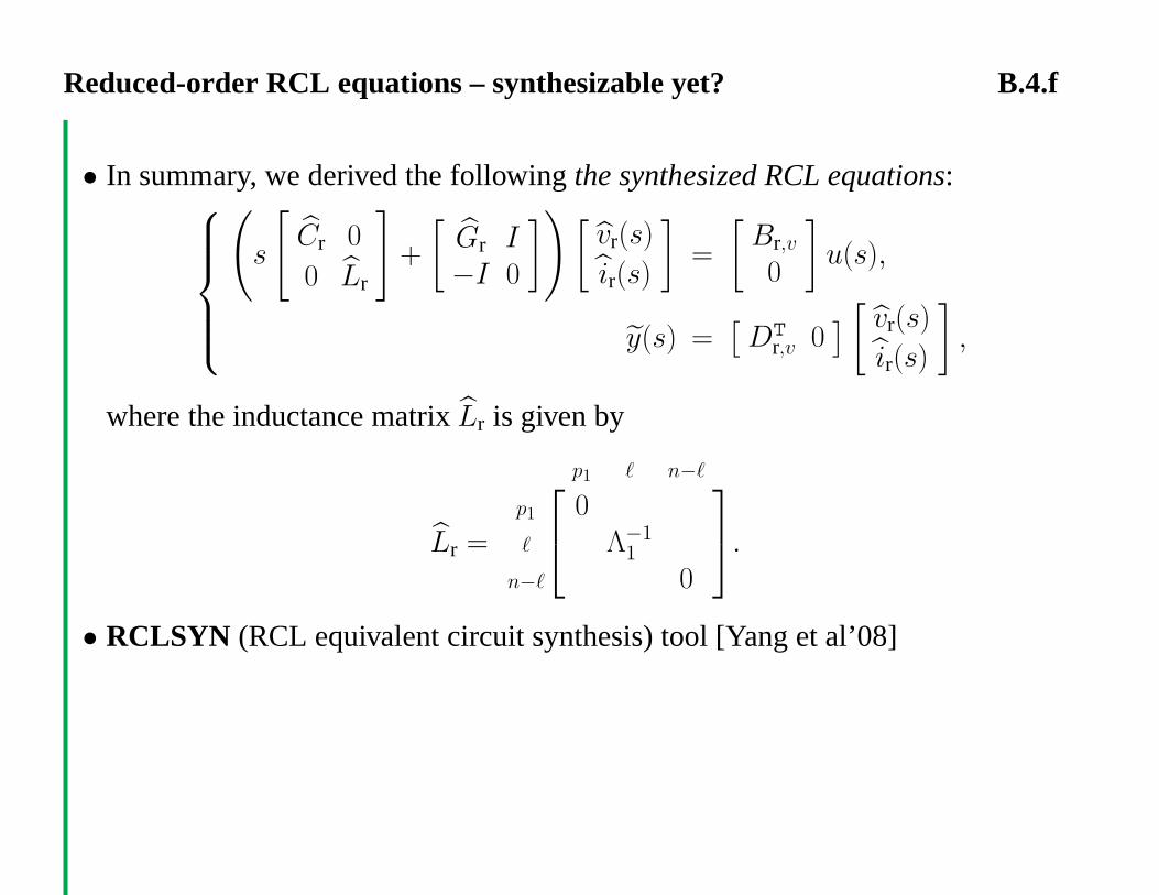
Reduced-order RCL equations – synthesizable yet? B.4.f
• In summary, we derived the following the synthesized RCL equations:⎧⎪⎪⎪⎨⎪⎪⎪⎩(
s
[Cr 0
0 Lr
]+
[Gr I−I 0
])[vr(s)
ir(s)
]=
[Br,v
0
]u(s),
y(s) =[DT
r,v 0] [ vr(s)
ir(s)
],
where the inductance matrix Lr is given by
Lr =
⎡⎣p1 � n−�
p1 0� Λ−1
1
n−� 0
⎤⎦.
• RCLSYN (RCL equivalent circuit synthesis) tool [Yang et al’08]

An example B.4.g
• A 64-bit bus circuit network with 8 inputs and 8 outputs.
• The order of the corresponding RCL circuit equation N = 16963.
• The order N of the synthesized RCL equations n = 640.
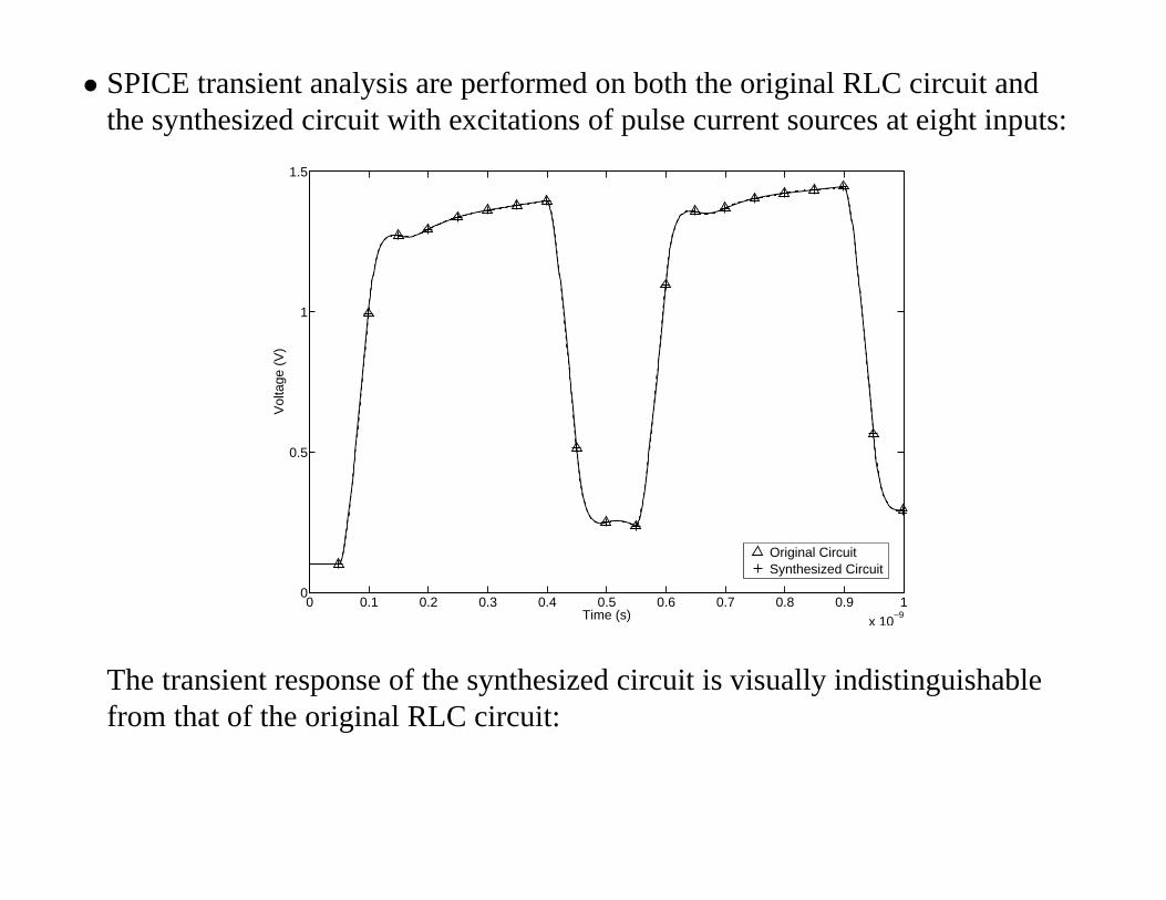
• SPICE transient analysis are performed on both the original RLC circuit andthe synthesized circuit with excitations of pulse current sources at eight inputs:
0 0.1 0.2 0.3 0.4 0.5 0.6 0.7 0.8 0.9 1
x 10−9
0
0.5
1
1.5
Time (s)
Vol
tage
(V
)
Original CircuitSynthesized Circuit
The transient response of the synthesized circuit is visually indistinguishablefrom that of the original RLC circuit:

• SPICE AC analysis was also performed on both the original RLC circuit andthe synthesized RLC circuit with current excitation at the near end of the firstline. The voltage at the far end of the first line is considered as the observingpoint.
0 1 2 3 4 5 6 7 8 9 10
x 109
8
10
12
14
16
18
20
Frequency (Hz)
Vol
tage
Mag
Original CircuitSynthesized Circuit
We see that two curves are visually indistinguishable.

• The CPU elapsed time for the transient and AC analysis are shown in thefollowing table:
Full RCL Synthesized RCL SpeedupDimensionality 16963 640Transient analysis 5007.59 (sec.) 90.16 (sec.) 50×AC analysis 29693.02 (sec.) 739.29 (sec.) 40×

Part C. Open problems and future development
Despite a lot of progress in Krylov subspace based SPMOR techniques, in recentyears, there are still many unsolved issues and open problems, such as
1. Automatic and adaptive choice of suitable expansion points s0
2. Robust and reliable stopping criteria and error bounds.
3. A fully synthesizable reduced-order RCL model
4. Development of a SPMOR method without using explicit subspace projectionso that it is appliable to truly large-scale systems.
5. Development of SPMOR techniques for systems with extreme large number ofI/O ports
6. Slow convergence reported in industrial practice: N = 106 → n = 103
References: [Freund’08] and [Schilders’08] ......

Part D. work in progress: SPMOR with optimal moment-matching
Open problem #4
All state-of-the-art SPMOR techniques are two-stage approach:
• generate a basis matrix of the underlying Krylov subspace
• emply explicit projection using some suitable partitioning of the basismatrix
Problems with such approach:
• storage of the basis matrix, which becomes prohibitive in the case oftruly large-scale problems,
• the reduced-order model are typically dense,
• the approximation properties are far from optimal (the available degreesof freedoms are not fully used).
Question: How to develop a structure-preserving moddel-order reduction methodthat avoid explicit projection?

Outline of Part D – work in progress: SPMOR with optimalmoment-matching
• Review of SISO second-order systems
• Structured Arnoldi decomposition and procedure
• SPMOR via Str-AR
• “Optimal” moment-matching property
• Preliminary numerical experiments
joint with Y. Li and W.-W. Lin of National Chiao Tung Univ., Taiwan

SISO second-order system
Consider a continuous time-invariant SISO second-order system of order N :
ΣN :
{Mx(t) + Dx(t) + Kx(t) = ru(t),
y(t) = wTx(t) + vTx(t),
with x(0) = x0 = 0 and x(0) = x0 = 0. Assume that K is nonsingular.
• An equivalent linear system:{Cq(t) + Gq(t) = b u(t),
y(t) = lTq(t),
where
C =
[D M−I 0
], G =
[K 00 I
], b =
[r0
], l =
[vw
], q(t) =
[x(t)x(t)
]• or {
Aq(t) + q(t) = bu(t),y(t) = lTq(t),
A = −G−1C =
[−K−1D −K−1MI 0
], b = G−1b =
[K−1r
0
]

Taking the Laplace transform of ΣN , we have{s2Mx(s) + sDx(s) + Kx(s) = ru(s),
y(s) = swTx(s) + vTx(s),
Transfer function:
h(s) = (swT + vT)(s2M + sD + K)−1r
= lT(sC + G)−1b
= lT(I− sA)−1b,
The power series expansion of h(s) at s = 0 is given by
h(s) = m0 + m1s + m2s2 + · · ·
=∞∑i=0
misi,
where mi are the moments:
mi = lTAib = lT(−G−1C)i(G−1b)
for i = 0, 1, 2, . . ..

Structure-preserving reduced order model
Seek a structure-preserving reduced order model of order n:
Σn :
{Mnξ(t) + Dnξ(t) + Knξ(t) = rnu(t),
η(t) = wTnξ(t) + vTnξ(t),
such that
• avoid explicit projection in defining system data matrices Mn,Dn,Kn andinput-output vectors rn,wn,vn.
• match 2n leading moments:
mi = m(n)i , for i = 0, 1, . . . , 2n− 1,
which impliesh(s) = hn(s) + O(s2n)

Structured Arnoldi decomposition
AX2n = X2n
[Rn Sn
Tn 0
]+ sn+1,nxn+1
where
• X2n is N × 2n
• xn+1 is N -vector
• Rn and Tn are n× n upper triangular matrices,
• Sn is an n× n upper Hessenberg matrix
[Rn Sn
Tn 0
]=
[�
�����
��
]

Structured Arnoldi decomposition and Krylov subspace
Structured Arnoldi decomposition:
AX2n = X2n
[Rn Sn
Tn 0
]+ sn+1,nxn+1
Krylov subspace
Kj(A;x1) = span{x1,Ax1,A2x1, . . . ,A
j−1x1}
Theorem. Suppose that a matrix X2n+1 = [X2n,xn+1 ] satisfies thestructured Arnoldi decomposition. Then we have
span{X2n} = K2n(A;x1)
andspan{X2n+1} = K2n+1(A;x1).

Structured Arnoldi procedure
• Assume that the Krylov subspace Kj(A;q1) is of dimension j forj = 2, 3, . . . 2n + 1, i.e., the matrix X2n+1 is of full column rank. (otherwise,breakdown will occur and can be treated)
• Partition X2n:X2n =
[Qn Pn
].
and denote x2n+1 = qn+1
• A Structured Arnoldi procedure can be derived to compute the structuredArnoldi decomposition satisfying the following orthogonality conditions:
1. QTn+1Qn+1 = In+1
2. Pn = In
3. pTi qj = 0 for i ≥ j

“Left projection matrix”
Define a “left projection matrix”
Y2n = X2n+1
(XT
2n+1X2n+1
)−1[I2n
0
].
Then
YT2nAX2n =
[Rn Sn
Tn 0
].
and
YT2nX2n = I2n
YT2nqn+1 = 0

Model order reduction via the Str-AR procedure
• Consider the linear system:{Aq(t) + q(t) = b0u(t)
y(t) = lTq(t),
where A = G−1C and b0 = G−1b.
• Let X2n = [Qn, Pn ] the basis matrix of K2n(A;b0) generated by thestructured Arnoldi procedure.
• By the change-of-variable
x(t) ≈ X2nz(t), z(t) ∈ R2n,
and “oblique” projection with the left projection matrix Y2n, we have{YT
2nAX2nz(t) + YT2nX2nz(t) = YT
2nb0u(t)η(t) = lTX2nz(t).
• By the fact
YT2nAX2n =
[Rn Sn
Tn 0
]and YT
2nb0 = γe1.

we have ⎧⎨⎩[Rn Sn
Tn 0
]z(t) +
[In 00 In
]z(t) = γe1u(t)
η(t) = lTX2nz(t).
• or equivalently,⎧⎪⎪⎨⎪⎪⎩[Rn −SnTn
−In 0
]z(t) +
[In 00 In
]z(t) = γe1u(t)
η(t) = lTX2n
[In 00 −Tn
]z(t).
where
z(t) =
[In 00 −T−1
n
]z(t).
• The above system can be rewritten as a second-order system of order n:
Σn :
{Mnξ(t) + Dnξ(t) + Knξ(t) = rnu(t),
η(t) = wTnξ(t) + vTnξ(t),
where the system matrices are Mn = −SnTn, Dn = Rn, Kn = In, and theinput and output vectors are rn = γe1, vn = QT
nl, wn = −TTnP
Tnl

The moment-matching property
Theorem. The first 2n moments of the original system ΣN and the reducedsystem Σn coincide:
mi = m(n)i for i = 0, 1, 2, . . . , 2n− 1,
which implies that
h(s) = hn(s) + O(s2n).

Example 1
• The vibration of a point-loaded semicircular shell coupled to an acoustic fluidfilling inside [Puri’08]
• For the undamped problem, it is an ABAQUS benchmark model termed as“acid-test” within the structural-acoustic community.
• N = 23412.
• Expansion point s0 = 2π × 103
• Comparison with SOAR and Q-Arnoldi [Meerbergen’08]

Low damping system: n = 200 (N = 23412)Str-AR vs. SOAR
100 200 300 400 500 600 700 800 900 1000−9
−8.5
−8
−7.5
−7
Frequency (Hz)
log1
0(M
agni
tude
)
Bode plot
ExactStr−ARSOAR
100 200 300 400 500 600 700 800 900 100010
−15
10−10
10−5
10−2
101
Frequency (Hz)
Rel
ativ
e er
ror
Str−ARSOAR

Low damping system: n = 200 (N = 23412)Str-AR vs. Q-Arnoldi
100 200 300 400 500 600 700 800 900 1000−9
−8.5
−8
−7.5
−7
Frequency (Hz)
log1
0(M
agni
tude
)
Bode plot
ExactStr−ARQ−Arnoldi
100 200 300 400 500 600 700 800 900 100010
−15
10−10
10−5
10−2
101
Frequency (Hz)
Rel
ativ
e er
ror
Str−ARQ−Arnoldi

Moderate damping system: n = 200 (N = 23412)Str-AR vs. SOAR
100 200 300 400 500 600 700 800 900 1000−9
−8.5
−8
−7.5
−7
Frequency (Hz)
log1
0(M
agni
tude
)
Bode plot
ExactStr−ARSOAR
100 200 300 400 500 600 700 800 900 100010
−15
10−10
10−5
10−2
101
Frequency (Hz)
Rel
ativ
e er
ror
Str−ARSOAR

Moderate damping system: n = 200 (N = 23412)Str-AR vs. Q-Arnoldi
100 200 300 400 500 600 700 800 900 1000−9
−8.5
−8
−7.5
−7
Frequency (Hz)
log1
0(M
agni
tude
)
Bode plot
ExactStr−ARQ−Arnoldi
100 200 300 400 500 600 700 800 900 100010
−15
10−10
10−5
10−2
101
Frequency (Hz)
Rel
ativ
e er
ror
Str−ARQ−Arnoldi

High damping system: n = 200 (N = 23412)Str-AR vs. SOAR
100 200 300 400 500 600 700 800 900 1000−8.8
−8.6
−8.4
−8.2
−8
−7.8
−7.6
Frequency (Hz)
log1
0(M
agni
tude
)
Bode plot
ExactStr−ARSOAR
100 200 300 400 500 600 700 800 900 100010
−15
10−10
10−5
10−2
101
Frequency (Hz)
Rel
ativ
e er
ror
Str−ARSOAR

High damping system: n = 200 (N = 23412)Str-AR vs. Q-Arnoldi
100 200 300 400 500 600 700 800 900 1000−8.8
−8.6
−8.4
−8.2
−8
−7.8
−7.6
Frequency (Hz)
log1
0(M
agni
tude
)
Bode plot
ExactStr−ARQ−Arnoldi
100 200 300 400 500 600 700 800 900 100010
−15
10−10
10−5
10−2
101
Frequency (Hz)
Rel
ativ
e er
ror
Str−ARQ−Arnoldi

Example 2.
• Acoustic analysis of fluid-structure interaction (by courtesy of Voith SimensHydro Power Generation GmbH & Co. KG)
• N = 89120.
• Profile of system matrices:
‖ · ‖1 sym. pos. def. nnzM 8.56× 10⁻² no no 3,207,494D 4.46× 10⁶ yes no 5,523,361K 2.80× 10¹⁰ no no 5,710,206
• Expansion point s0 = 2π × 50

14
Fluid Structure Interaction at Acoustic Level
By courtesy of Voith Siemens Hydro Power Generation By courtesy of Voith Siemens Hydro Power Generation GmbH & Co. KGGmbH & Co. KG

Relative error of n = 100 (N = 89120)Str-AR vs. SOAR vs. Q-Arnoldi
0 50 100 150 200 25010
−15
10−10
10−5
10−2
100
Frequency (Hz)
Rel
ativ
e er
ror
Str−ARSOARQ−Arnoldi

Recap
A. A unified theory for SPMOR
Basic formulation, a genric algorithm, structure of Krylov subspace, structuredArnoldi process
B. Case study: RCL/RCS circuits
Towards synthesizable reduced-order RCL circuits
C. Open problems and future development
D. Working in progress: SPMOR with optimal moment-matching
avoiding explicit projection