structure tensor based image interpolation method · structure tensor based image interpolation...

Structure Tensor Based Image Interpolation Method

Ahmadreza Baghaie and Zeyun Yu

University of Wisconsin-Milwaukee, WI, USA

Abstract — Feature preserving image interpolation is an active area in image processing field. In

this paper a new direct edge directed image super-resolution algorithm based on structure tensors is

proposed. Using an isotropic Gaussian filter, the structure tensor at each pixel of the input image is

computed and the pixels are classified to three distinct classes; uniform region, corners and edges,

according to the eigenvalues of the structure tensor. Due to application of the isotropic Gaussian filter,

the classification is robust to noise presented in image. Based on the tangent eigenvector of the

structure tensor, the edge direction is determined and used for interpolation along the edges. In

comparison to some previous edge directed image interpolation methods, the proposed method

achieves higher quality in both subjective and objective aspects. Also the proposed method

outperforms previous methods in case of noisy and JPEG compressed images. Furthermore, without

the need for optimization in the process, the algorithm can achieve higher speed1.

.

Index Terms — Local structure tensor, Image interpolation, Super-Resolution, Edge-directed

interpolation

1. INTRODUCTION

Feature preserving image interpolation is an active area in the image processing field,

from everyday digital pictures to application-oriented medical and satellite images. Many

methods have been proposed in the past decades to tackle this problem [1-20]. Generally

speaking, the methods for image interpolation/super-resolution can be divided in 3 different

categories: 1) Direct Interpolation methods, 2) PDE based interpolation methods and 3)

Optimization based interpolation methods. All of these methods have their pros and cons

regarding their simplicity of implementation, computational complexity and performance.

The proposed method in this paper is a direct interpolation method without the need for any

optimization in the process. Also in terms of computational time, the proposed method can

achieve the result in less than one second for an image of typical size using MEX based

implementation. This feature along with not using any optimization procedure, as well as

being robust in case of noisy images, make this method a suitable choice for implementation

in everyday used electronic devices.

Nearest neighbor and bilinear interpolation are two simple methods for image

interpolation [1]. Despite the simplicity in implementation and very low computational cost,

these methods suffer from severe blocky artifacts, as well as blurring and ringing artifacts

near the edges. Although better performance can be achieved by using higher order splines,

rather than 0 and 1 order splines as in the nearest neighbor and bilinear methods, higher

order spline methods still contain oscillatory edges and ringing artifacts [2]. The main

reason is that these methods don’t take into consideration any information other than

intensity values. In other words, they are intensity based and not feature (edge) based. So

even though they are easy to implement and need low computational cost, they are not

suitable for most of applications.

The final recipient of any image processing algorithm is the human visual system which is

1 Ahmadreza Baghaie (Corresponding author) is with the Department of Electrical Engineering at University of

Wisconsin - Milwaukee, Milwaukee, WI 53211 ([email protected]).

Zeyun Yu is with the Department of Computer Science at University of Wisconsin - Milwaukee, Milwaukee, WI 53211

([email protected]).

very feature sensitive. These features are mostly edges and corners within the image. Also

sharpness of the final image is of high importance. Based on these criteria, the previously

mentioned methods, despite their technical advantages, are not satisfactory. So the need for

introducing new approaches and novel models for image interpolation which satisfy the

human visual system has been emerged in the past decades and many methods have been

proposed. Some of these methods will be mentioned here.

Edge directed methods usually are the first ones that come to notice when dealing with

image interpolation problem. In 2001 a method called NEDI was proposed which performs

based on the assumption that every image can be modeled as a locally stationary Gaussian

process [3]. Based on this assumption, the local covariance coefficients from the low

resolution (LR) image is estimated and then interpolation is done based on the geometric

duality between the LR covariance and the high resolution (HR) covariance. An improved

version of NEDI algorithm called iNEDI is proposed later which achieves higher scores in

terms of subjective and objective image quality measures relative to NEDI with the cost of

needing more computational time [4]. Another edge directed image interpolation method is

ICBI which works based on an estimation of the edge orientation using second order

derivative of the image [5]. DFDF method [6] is another method in this category which

utilizes directional filtering and data fusion. In DFDF, at first, two observation sets are

defined in two orthogonal directions for each pixel to be interpolated. Then these two

estimates will be fused using Linear Minimum Mean Square Error (LMMSE) in order to

achieve a more robust estimate for the missing pixel.

Methods proposed in [7-15] also are good examples of edge directed image interpolation.

In [7], the method is based on partitioning the input image into homogeneous and edge areas

with regard to local structure of the image and then, interpolating each parts differently,

bilinear interpolation for homogeneous regions and an adaptive edge oriented method for

edge pixels. In [8], a modified edge adaptive bilinear image interpolation method called EASE

is proposed. This modified version is achieved using the classical interpolation error

theorem. In [9], a new directional cubic convolution (CC) interpolation scheme is proposed.

In [10], an interpolation framework is proposed in which denoising and image sharpening

are embedded together. In this method, bilateral filtering method is used to partition the

input image into detail and base layers, and then edge preserving interpolation method is

applied to each layer. In [11], the edge information of the LR image is first estimated using

the modified Leung-Malik filter bank, and then this information is converted into that of HR

image by using a mapping function. In [12], a fast image interpolation method with adaptive

weights is proposed motivated by Inverse Distance Weighting (IDW). The use of Radial Basis

Functions (RBFs) to solve image interpolation problem is investigated in [13, 14]. In [15], a

soft decision interpolation technique is proposed which estimates missing pixels in groups

rather than one at a time. They use a piecewise 2-D autoregressive (AR) model to determine

the local structure of the scene.

Even though the above mentioned methods are of a wide range of use and discipline, still

there are more methods that are not discussed here; like Partial Differential Equation (PDE)

based methods [16, 17, 27], and regularization based methods [18-20]. The reader will be

referred to the papers and their references for more information on these classes of image

interpolation methods.

As can be seen, each of the mentioned methods deals with the image interpolation

problem from a different angle. But still image interpolation is an open problem and there is

room for improvement. In this paper, a new edge-directed method based on structure tensor

will be proposed which its strength is not only in reconstructing edges in the HR image, but

also is more robust in case of noise. The proposed method is very simple and easy to

implement and based on the conducted experiments, outperforms the most common image

interpolation methods. For comparison, five well-known image interpolation methods are

considered: NEDI [3], DFDF [5], ICBI [6], KR [26] and iNEDI [4]. Tests were conducted for

noise-free, noisy and JPEG compressed images. For completeness of the comparison another

structure tensor-based method by Roussos and Maragos [27] is also considered. This

method (RM) can be categorized as a PDE-based technique. In this method at first an initial

interpolation is done by Fourier zero-padding and de-convolution. The result of this stage

suffers from significant ringing artifacts. Using a tensor-driven diffusion process, the ringing

artifacts are removed. The main assumption in this method is that the process of

interpolation is a reversible process which cannot be hold always. Based on this assumption,

interpolation is done by first applying an anti-aliasing low-pass filter followed by sampling.

This assumption can be problematic especially in the case of naïve sub-sampling which is the

case used in this paper. In naïve sub-sampling of factor �, one pixel is chosen from each �

pixels of the image without any anti-aliasing filtering. This will cause high amount of ringing

artifacts near edges introduced by the first stage of the method as well as sever stair-cased

edges which cannot be resolved properly using the tensor-driven diffusion process. More

discussion will be given in the following sections regarding this issue. Here the online

implementation of this method is used implemented by Getreuer [28].

The rest of the paper is organized as follows: in Section 2 a brief introduction will be given

on structure tensor computation and its theoretical aspects. Then in Section 3, the proposed

interpolation method will be described in more detail. Section 4 contains the

implementation aspects, image quality measures that being used and tables of objective and

subjective comparison between the five above mentioned methods and the proposed

method, as well as some of the final results. Section 5 concludes the paper.

2. LOCAL STRUCTURE TENSOR

Local structure tensors have been used in image processing to solve problems such as

anisotropic filtering [21, 22] and motion detection [23]. This method uses the gradient

information of an image in order to determine the orientation information of the edges and

corners. The structure tensor is defined as:

�� = � �� ∗ � �� ∗ �� ∗ � �� ∗ � � = �� (1)

where � is a Gaussian function with standard deviation σ, and�� and ��are horizontal

and vertical components of the gradient vector at each pixel respectively. Since matrix �� is

symmetric and positive semi-definite, it has two orthogonal eigenvectors as follows:

� = �� − �� + �(�� − ��)� + 4��−2�� ,andnormalizedas:� = �‖�‖(2) �* = � 2�� − �� + �(�� − ��)� + 4�� ,andnormalizedas:�* = �*‖�*‖(3)

The corresponding eigenvalues for each eigenvector are as follows:

, = 12-�� + �� − �(�� − ��)� + 4�� .(4)

,* = 12-�� + �� + �(�� − ��)� + 4�� .(5)

Apparently the eigenvalue d is smaller than ,*. Based on the two eigenvalues, local

structures can be determined as one of three types:

• Constant areas: ,* ≈ , ≈ 0

• Edges: ,* ≫ , ≈ 0

• Corners: ,* ≈ , ≫ 0

For edge points, the eigenvector�corresponding to the smaller eigenvalue is along the

edge (tangent direction), while the eigenvector �*is across the edge (normal direction).

Although using gradient vectors in an image can determine the edge orientations

too, there are some other advantages in using structure tensors compared to gradient

vectors alone. First, the edges in an image may not be smooth and continuous, especially in

down-sampled images. With the Gaussian filtering of the gradient vectors in a neighborhood,

as seen in the definition of the structure tensor, one can acquire more robust and accurate

estimation of edge orientations. Second, the structure tensor can classify local features into

several distinctive types, which is nontrivial by using gradient vectors alone. This becomes

more obvious when a three-dimensional image or cloud of points is being considered. Also

because of the Gaussian filtering stage, the edge orientation achieved by structure tensor is

more robust against noise.

3. METHODOLOGY

3.1 Structure Tensor Based Image Interpolation

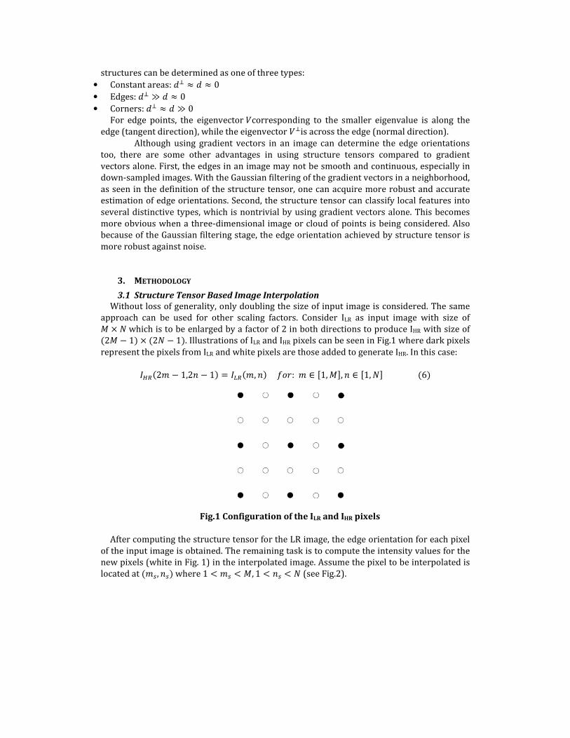
Without loss of generality, only doubling the size of input image is considered. The same

approach can be used for other scaling factors. Consider ILR as input image with size of 3 × �which is to be enlarged by a factor of 2 in both directions to produce IHR with size of (23 − 1) × (2� − 1). Illustrations of ILR and IHR pixels can be seen in Fig.1 where dark pixels

represent the pixels from ILR and white pixels are those added to generate IHR. In this case:

567(28 − 1,29 − 1) = 5:7(8, 9);<=:8 ∈ ?1,3@, 9 ∈ ?1, �@(6)

Fig.1 Configuration of the ILR and IHR pixels

After computing the structure tensor for the LR image, the edge orientation for each pixel

of the input image is obtained. The remaining task is to compute the intensity values for the

new pixels (white in Fig. 1) in the interpolated image. Assume the pixel to be interpolated is

located at (8B, 9B) where 1 < 8B < 3, 1 < 9B < � (see Fig.2).

Fig.2 Configuration of the new pixel at location (DE, FE) w.r.t known pixels from

input image

The intensity value for the pixel to be interpolated is defined as a weighted summation of

pixels in a defined neighborhood. Here a square neighborhood for averaging is defined. The

complete form of the weighted average is:

567(28B − 1, 29B − 1) = G G HI(J, K)HL(J, K)5:7(J, K)(7)NOPQRS

TUNOPQVSNWPQRS

XUNWPQVS

where D is half of the neighborhood size and HI and HL are weight functions. HIis the

distance based part of the weight function and it can be defined for pixel (i,j) in the

neighborhood as follows:

HI(J, K) = YVZ[\]V^_`\a(8)

where C is the location of nearest pixel to (8B, 9B):c = (N8BQ, N9BQ) and dXT is the location

of pixel (i,j) in the neighborhood (see Fig.2). HLis the structure tensor based part of the

weight function.

As previously mentioned, the eigenvalues and eigenvectors of the structure tensor at a

pixel can be used to determine the tangent and normal directions at the pixel in the input

image. To reduce the staircase artifact in the interpolated image, the interpolation should be

performed along the edges. For this reason, the tangent eigenvector is used as a measure for

computing the weight HL . As shown in Fig.2 where the pixel at (8B, 9B) needs to be

interpolated, for every pixel with known intensity value in the neighborhood, a vector

connecting (8B, 9B) to the pixel can be defined. The corresponding weight is defined in such

a way that only pixels with similar edge direction as the connecting vector should be

assigned higher weights. In other words, even though the defined neighborhood is isotropic,

the shape of the structure tensor based weight is not symmetric, unlike the distance based

weight function. Therefore HL is defined as follows:

HL(J, K) = YefIgh-i_`,[]V^_`a\]V^_`\.f(9)

Where �XT is the tangent eigenvector of the pixel at (i, j) in the neighborhood and the dot

denotes the dot product of two normalized input vectors.

Using this formulation for computing the total weight, not only the distance between the

pixel to be interpolated and its neighboring pixels but also the edge orientation of the

neighboring pixels are taken into consideration. The main difference between this method

and other gradient based methods is that the edge orientation is achieved using structure

tensors and thus the blocky artifacts are significantly reduced.

3.2 Implementation

Apparently a straightforward implementation of the proposed algorithm can be very time

consuming. For example, assuming a 5x5 neighborhood size for each new pixel to be

interpolated, 25 weights for each of the distance based and structure tensor based weights

should be computed before the computation of the weighted summation. Fortunately, in

most digitized images, only a small portion of pixels are edge/corner regions leaving a large

number of pixels in uniform regions with very small variations in gray values. These regions

don’t contain as much important information as edges/corners and hence they can be easily

and efficiently interpolated using simple and fast interpolation methods like bilinear

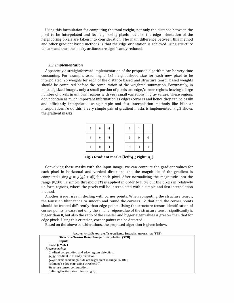
interpolation. To do this, a very simple pair of gradient masks is implemented. Fig.3 shows

the gradient masks:

Fig.3 Gradient masks (left:kl; right: km)

Convolving these masks with the input image, we can compute the gradient values for

each pixel in horizontal and vertical directions and the magnitude of the gradient is

computed using k = n(�� + ��) for each pixel. After normalizing the magnitude into the

range [0,100], a simple threshold (T) is applied in order to filter out the pixels in relatively

uniform regions, where the pixels will be interpolated with a simple and fast interpolation

method.

Another issue rises in dealing with corner points. When computing the structure tensor,

the Gaussian filter tends to smooth and round the corners. To that end, the corner points

should be treated differently than edge points. Using the structure tensor, identification of

corner points is easy: not only the smaller eigenvalue of the structure tensor significantly is

bigger than 0, but also the ratio of the smaller and bigger eigenvalues is greater than that for

edge pixels. Using this criterion, corner points can be detected.

Based on the above considerations, the proposed algorithm is given below.

ALGORITHM 1: STRUCTURE TENSOR BASED IMAGE INTERPOLATION (STB)

Structure Tensor Based Image Interpolation (STB)

Inputs:

ILR, D, β, γ, σ, T

Preprocessing:

Gradient computation and edge regions detection:

gx, gy: Gradient in x and y direction

gmag: Normalized magnitude of the gradient in range [0, 100]

IE: Image’s edge map, using threshold T

Structure tensor computation:

Defining the Gaussian filter using σ;

Computing o, o*, p, p*

Interpolation:

For i=D+1to M-D with step=1/2

For j=D +1to N-D with step=1/2

If NJQ = Jq9,NKQ = K rst(uv − w, ux − w) = ryt(v, x); Else if c = (N8BQ, N9BQ) is in uniform region or is a corner point

Bilinear Interpolation;

Else

rst(uDE − w, uFE − w) = ∑ ∑ {o(v, x){|(v, x)ryt(v, x)NFEQR}xUNFEQV}NDEQR}vUNDEQV}

End

End

End

4 EXPERIMENTAL RESULTS

4.1 Image Quality Measures

In order to assess the proposed algorithm, several image quality measures were used. The

most popular measure is Peak Signal to Noise Ratio (PSNR) which measures the intensity

differences between two images [24]. Assume that X is the original image, and Y is the

reconstructed image from the downsampled version. The Mean Squared Error (MSE)

between X and Y is defined as follows:

3~� = 1�G(�X − �X)�(10)�XU�

Where �X and �X are the ith pixel of the original and reconstructed image respectively and N

is the total number of pixels. Based on MSE, PSNR is defined as follows:

d~�� = 10�<�� 3~�(11)

where L is the dynamic range of pixel intensities in the images.

Another measure that is used is Edge PSNR (EPSNR) which is defined in the same manner

as above, but instead uses the edge maps of the original and reconstructed images. For edge

map computation, a simple Sobel operator is used.

Even though PSNR and EPSNR are proper measures for image quality comparison, they

are objective and usually fail in describing the visual perception of images. To remedy this

problem, several subjective image quality measures were proposed in literature. A well-

known measure is the Structural SIMilarity(SSIM) index [24]. Recently another method

called Feature SIMilarity (FSIM) index is proposed for image quality comparison [25]. In the

following, these four measures are used to assess and compare the proposed method and

several other interpolation techniques.

4.2 Results and Comparisons

In order to evaluate the performance of the proposed method, several images were tested.

Fig.4 displays the test images considered in this paper. For each image, a direct

downsampling procedure with a factor of 2 is performed in order to produce the ILR image.

Then with the STB interpolation method the images were enlarged.

The performance of our algorithm is tested, using both noise-free and noisy images. For

noisy images, compressed images are considered for comparison. JPEG format with 75% as

quality is used here. Also for completeness of the experiments, our algorithm is also tested

on images with added Gaussian noise. Tables 1

measures of the proposed method in comparison with several popular image interpolation

methods for noise free images. For all of methods the default parameters are used. The

default parameters for STB method are as follows:

As can be seen from Tables 1

other methods. On the other hand, RM method performs poorly mainly because of the

assumption of reversible interpolation. This assumption cannot be h

sampling which is the case here. This is mainly due to the Fourier zero

convolution in the first stage of the algorithm which causes significant ringing artifacts near

edges. On some of the images, the iNEDI approach also works well.

does not perform as well as our method when dealing with compressed images. Table 3

represents the objective and subjective comparisons between STB and iNEDI for

compressed images.

For comparing the results of the proposed algorithm vs. iNEDI in case of noisy images, an

additive Gaussian noise (zero mean with 0.1% variance) is applied to downsampled images,

and then used our method and iNEDI to produce the enlarged images. Table

the results of objective and subjective image quality measures for test images.

As can be seen in Table 4, the STB outperforms iNEDI in almost all of the images with

noticeable margin. Fig 5-6 show the overall results of different interpolati

some of the test images.

Fig.4 Images used for comparison, from left to right, top to bottom: Airplane (512x768),

(324x492), Door (512x512), Flowers (480x640), Girl (512x

TABLE 1 :OBJECTIVE

Method NEDI

PSNR EPSNR

DFDF

PSNR EPSNR

Airplane

Lena

Flowers

Girl

Door

Splash

Butterfly

28.69 15.42

33.57 27.75

25.62 19.94

31.84 28.30

32.14 25.73

31.38 15.49

28.96 21.02

30.53 19.44

33.96 28.10

25.74 20.40

31.81 29.41

32.27 25.93

33.79 19.79

29.67 20.76

on images with added Gaussian noise. Tables 1-2 represent objective and subjective



default parameters for STB method are as follows: σ= 2, D=2, β=5, γ=10, T=20.

As can be seen from Tables 1-2, the STB method performs very well in comparison with

On the other hand, RM method performs poorly mainly because of the

assumption of reversible interpolation. This assumption cannot be hold in case of naïve sub

sampling which is the case here. This is mainly due to the Fourier zero-padding and de


On some of the images, the iNEDI approach also works well. However, this method





and then used our method and iNEDI to produce the enlarged images. Table 4 summarizes

the results of objective and subjective image quality measures for test images.


6 show the overall results of different interpolation methods on

Fig.4 Images used for comparison, from left to right, top to bottom: Airplane (512x768), Butterfly

), Flowers (480x640), Girl (512x512), Lena (512x512), Splash (512x768)

BJECTIVE QUALITY COMPARISON OF DIFFERENT INTERPOLATION METHODS

PSNR EPSNR

ICBI

PSNR EPSNR

KR

PSNR EPSNR

RM

PSNR EPSNR

iNEDI

PSNR EPSNR

30.53 19.44

33.96 28.10

25.74 20.40

31.81 29.41

32.27 25.93

19.79

29.67 20.76

30.08 18.68

34.05 26.99

25.20 19.24

31.27 28.82

31.71 24.33

33.32 21.29

29.91 20.26

29.11 16.01

33.97 27.97

25.79 20.23

31.92 29.10

32.20 25.86

33.38 19.07

29.54 21.25

27.64 18.28

30.41 24.89

22.61 17.60

29.02 26.46

28.56 22.42

32.45 20.55

27.15 18.79

30.66 19.65

34.11

25.89 20.66

32.24

32.41 25.99

33.69 21.28

30.07

objective and subjective



2, the STB method performs very well in comparison with

On the other hand, RM method performs poorly mainly because of the

old in case of naïve sub-

padding and de-


However, this method





4 summarizes


on methods on

Butterfly

), Lena (512x512), Splash (512x768)

iNEDI

PSNR EPSNR

STB

PSNR EPSNR

30.66 19.65

27.86

20.66

29.30

32.41 25.99

21.28

30.07 21.36

30.71 19.82

33.99 28.70

26.01 20.78

31.99 29.46

32.47 26.25

35.23 21.26

29.31 21.49

TABLE 2: SUBJECTIVE QUALITY COMPARISON OF DIFFERENT INTERPOLATION METHODS

Method NEDI

SSIM FSIM

DFDF

SSIM FSIM

ICBI

SSIM FSIM

KR

SSIM FSIM

RM

SSIM FSIM

iNEDI

SSIM FSIM

STB

SSIM FSIM

Airplane

Lena

Flowers

Girl

Door

Splash

Butterfly

.9110 .9782

.9112 .9862

.6884 .9412

.7842 .9684

.8576 .9621

.9285 .9829

.9427 .9462

.9144 .9804

.9129 .9871

.6844 .9390

.7741 .9656

.8607 .9637

.9296 .9629

.9501 .9546

.9085 .9781

.9112 .9868

.6651 .9316

.7523 .9590

.8501 .9575

.9241 .9826

.9513 .9549

.9049 .9798

.9097 .9875

.6648 .9440

.7675 .9701

.8501 .9633

.9245 .9824

.9468 .9464

.8606 .9710

.8448 .9807

.5914 9143

.7055 .9464

.7570 .9506

.8677 .9783

.9099 .9221

.9166 .9811

.9175 .9876

.6974 .9428

.7933 .9717

.8625 .9622

.9328 .9852

.9507 .9518

.9177 .9815

.9147 .9875

.6940 .9450

.7805 .9698

.8662 .9631

.9313 .9836

.9475 .9498

TABLE 3: OBJECTIVE AND SUBJECTIVE QUALITY COMPARISON FOR COMPRESSED IMAGES

Method iNEDI

PSNR EPSNR SSIM FSIM

STB


Airplane

Lena

Flowers

Girl

Door

Splash

Butterfly

29.84 19.34 0.8803 0.9716

32.54 26.73 0.8773 0.9789

25.20 20.33 0.6362 0.9320

31.24 28.14 0.7468 0.9646

31.26 25.24 0.8009 0.9493

33.38 20.04 0.8908 0.9758

29.09 21.01 0.9185 0.9277

30.50 19.76 0.9104 0.9804

33.78 28.49 0.9097 0.9892

25.37 20.22 0.6729 0.9273

32.44 29.57 0.7931 0.9809

32.28 26.19 0.8536 0.9643

33.56 19.87 0.9242 0.9824

29.04 21.22 0.9408 0.9433

Average 30.36 22.97 0.8215 0.9571 30.99 23.61 0.8578 0.9668

TABLE 4: OBJECTIVE AND SUBJECTIVE QUALITY COMPARISON FOR NOISY IMAGES

Method iNEDI


STB


Airplane

Lena

Flowers

Girl

Door

Splash

Butterfly

28.71 19.46 0.7638 0.9050

29.84 26.28 0.7409 0.9274

24.74 20.22 0.6106 0.9036

28.90 27.29 0.6518 0.9175

29.15 25.01 0.6631 0.8976

30.51 20.93 0.7108 0.9024

27.84 20.85 0.7767 0.8860

28.79 19.50 0.7660 0.9063

30.17 27.15 0.7469 0.9344

25.10 20.44 0.6201 0.9159

29.24 27.76 0.6583 0.9256

29.47 25.34 0.6760 0.9056

30.69 20.94 0.7206 0.9107

27.58 21.09 0.7793 0.8844

Average 28.53 22.87 0.7025 0.9056 28.73 23.18 0.7096 0.9118

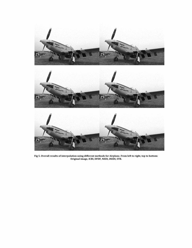
Fig 5. Overall results of interpolation using different methods for Airplane. From left to right, top to bottom:

Original image, ICBI, DFDF, NEDI, iNEDI, STB.

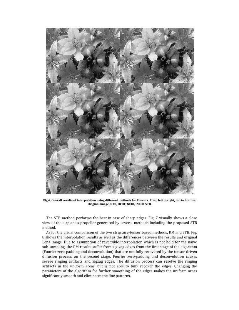
Fig 6. Overall results of interpolation using different methods for Flowers. From left to right, top to bottom:

Original image, ICBI, DFDF, NEDI, iNEDI, STB.

The STB method performs the best in case of sharp edges. Fig. 7 visually shows a close

view of the airplane’s propeller generated by several methods including the proposed STB

method.

As for the visual comparison of the two structure-tensor based methods, RM and STB, Fig.

8 shows the interpolation results as well as the differences between the results and original

Lena image. Due to assumption of reversible interpolation which is not hold for the naïve

sub-sampling, the RM results suffer from zig-zag edges from the first stage of the algorithm

(Fourier zero-padding and deconvolution) that are not fully recovered by the tensor-driven

diffusion process on the second stage. Fourier zero-padding and deconvolution causes

severe ringing artifacts and zigzag edges. The diffusion process can resolve the ringing

artifacts in the uniform areas, but is not able to fully recover the edges. Changing the

parameters of the algorithm for further smoothing of the edges makes the uniform areas

significantly smooth and eliminates the fine patterns.

Another important aspect of image interpolation methods is the computational cost. This

has become more important when images are now digitized in much higher resolutions.

Table 5 shows the average computational time for the test images using different methods.

The RM method is excluded from this table since the available implementation is in C and

not MATLAB. The tests were performed on a 3GHz Intel Core 2 Duo desktop with 4 GB of

RAM. It can be seen that the proposed STB method is the fastest as compared to several

other popular approaches. To further reduce the time cost, especially for some real-time

applications, a MEX version of the proposed algorithm is implemented and the

computational time was reduced to less than 1 second.

TABLE 5: COMPARISON OF AVERAGE COMPUTATIONAL TIME FOR DIFFERENT METHODS

Method NEDI DFDF ICBI iNEDI STB

Time (sec) 21.5 19.6 127.4 800.2 11.4

4. CONCLUSION

In this paper, a new edge directed method for image interpolation based on structure is

proposed which takes into account the advantages of structure tensor to determine the edge

orientation as well as corner points of an image. Even though the concept of structure tensor

is the same as gradient vectors, due to the presence of noise and discontinuity of edges

caused by image compression, downsampling and digitizing, the structure tensor provides

more robust edge orientations. Also using structure tensor, corner points can be better

distinguished from other features such as edges.

The proposed method is tested for noise-free, noisy and JPEG compressed images.

Numerous comparisons were made against several popular image interpolation methods. In

most cases the proposed method outperformed the other methods both subjectively and

objectively, especially in case of noisy and compressed images with noticeable margin. Also

in terms of computational time, the proposed method can achieve the result in less than one

second for an image of typical size using MEX based implementation. This feature along with

not using any optimization procedure, as well as being robust in case of noisy images, make

this method a suitable choice for implementation in everyday used electronic devices; Not to

forget parallelizability using GPU based implementations.

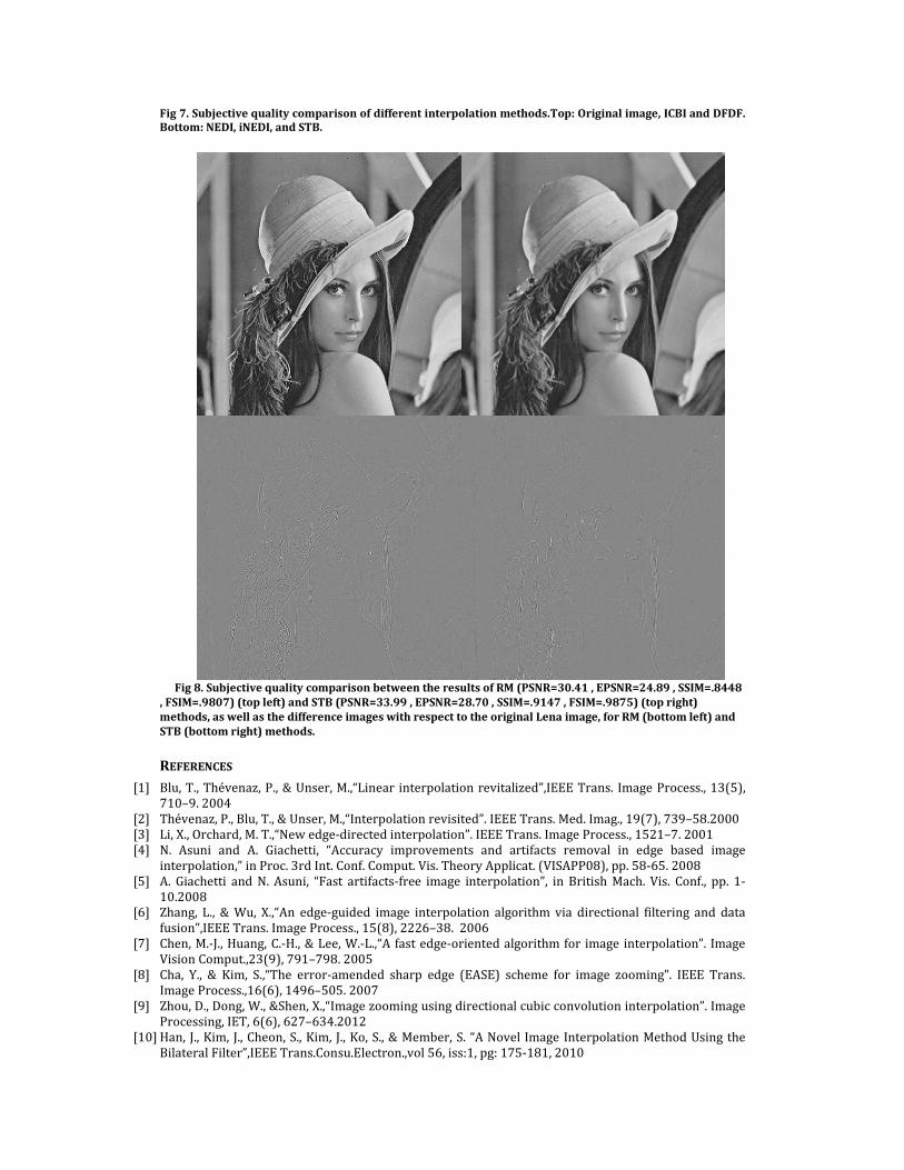
Fig 7. Subjective quality comparison of different interpolation methods.Top: Original image, ICBI and DFDF.

Bottom: NEDI, iNEDI, and STB.

Fig 8. Subjective quality comparison between the results of RM (PSNR=30.41 , EPSNR=24.89 , SSIM=.8448

, FSIM=.9807) (top left) and STB (PSNR=33.99 , EPSNR=28.70 , SSIM=.9147 , FSIM=.9875) (top right)

methods, as well as the difference images with respect to the original Lena image, for RM (bottom left) and

STB (bottom right) methods.

REFERENCES

[1] Blu, T., Thévenaz, P., & Unser, M.,“Linear interpolation revitalized”,IEEE Trans. Image Process., 13(5),

710–9. 2004

[2] Thévenaz, P., Blu, T., & Unser, M.,“Interpolation revisited”. IEEE Trans. Med. Imag., 19(7), 739–58.2000

[3] Li, X., Orchard, M. T.,“New edge-directed interpolation”. IEEE Trans. Image Process., 1521–7. 2001

[4] N. Asuni and A. Giachetti, “Accuracy improvements and artifacts removal in edge based image

interpolation,” in Proc. 3rd Int. Conf. Comput. Vis. Theory Applicat. (VISAPP08), pp. 58-65. 2008

[5] A. Giachetti and N. Asuni, “Fast artifacts-free image interpolation”, in British Mach. Vis. Conf., pp. 1-

10.2008

[6] Zhang, L., & Wu, X.,“An edge-guided image interpolation algorithm via directional filtering and data

fusion”,IEEE Trans. Image Process., 15(8), 2226–38. 2006

[7] Chen, M.-J., Huang, C.-H., & Lee, W.-L.,“A fast edge-oriented algorithm for image interpolation”. Image

Vision Comput.,23(9), 791–798. 2005

[8] Cha, Y., & Kim, S.,“The error-amended sharp edge (EASE) scheme for image zooming”. IEEE Trans.

Image Process.,16(6), 1496–505. 2007

[9] Zhou, D., Dong, W., &Shen, X.,“Image zooming using directional cubic convolution interpolation”. Image

Processing, IET, 6(6), 627–634.2012

[10] Han, J., Kim, J., Cheon, S., Kim, J., Ko, S., & Member, S. “A Novel Image Interpolation Method Using the

Bilateral Filter”,IEEE Trans.Consu.Electron.,vol 56, iss:1, pg: 175-181, 2010

[11] Han, J.-W., Kim, J.-H., Sull, S., &Ko, S.-J. “New edge-adaptive image interpolation using anisotropic

Gaussian filters”. Digit Signal Process.,23(1), 110–117.2013

[12] Jing, M., & Wu, J. “Fast image interpolation using directional inverse distance weighting for real-time

applications”. Opt Commun.,286, 111–116.2013

[13] Lee, Y. J., & Yoon, J. “Nonlinear image upsampling method based on radial basis function interpolation”.

IEEE Trans. Image Process.,19(10), 2682–92.2010

[14] Casciola, G., Montefusco, L. B., &Morigi, S. “Edge-driven Image Interpolation using Adaptive Anisotropic

Radial Basis Functions”. J Math Imaging Vis., 36(2), 125–139. 2009

[15] Zhang, X., & Wu, X. “Image interpolation by adaptive 2-D autoregressive modeling and soft-decision

estimation”. IEEE Trans. Image Process.,17(6), 887–96. 2008

[16] Shao, W.-Z., & Wei, Z.-H. “Edge-and-corner preserving regularization for image interpolation and

reconstruction”.Image Vision Comput.,26(12), 1591–1606. 2008

[17] Kim, H., Cha, Y., & Kim, S. “Curvature interpolation method for image zooming”. IEEE Trans. Image

Process., 20(7), 1895–903. 2011

[18] El-Khamy, S. E., Hadhoud, M. M., Dessouky, M. I., Salam, B. M., Abd El-Samie, F. E. “Efficient

implementation of image interpolation as an inverse problem”. Digit Signal Process.,15(2), 137–

152.2005

[19] Liu, X., Zhao, D., Xiong, R., Ma, S., Gao, W., & Sun, H. “Image interpolation via regularized local linear

regression”. IEEE Trans. Image Process.,20(12), 3455–69.2011

[20] Liu, Z. “Adaptive regularized image interpolation using a probabilistic gradient measure”. Opt

Commun.,285(3), 245–248., 2012

[21] J.-J. Fernandez and S. Li, “An improved algorithm for anisotropic nonlinear diffusion for denoising cryo-

tomograms”, J StructBiol, vol. 144, pp. 152-161, 2003

[22] Weickert, J., Anisotropic Diffusion In Image Processing, Teubner-Verlag, Stuttgart, 1998

[23] Khne, G., Weickert, J., Schuster, O., Richter, S., "A tensor-driven active contour model for moving object

segmentation", in Proc. Int. Conf. Image Processing, 2001, pp. 73-76. 2001

[24] Zhou Wang, Alan C. Bovik, Modern Image Quality Assessment. Synthesis Lectures on Image, Video, and

Multimedia Processing, Morgan & Claypool Publishers, 2006

[25] L. Zhang, L. Zhang, X. Mou, and D. Zhang,“FSIM: A feature similarity index for image quality assessment”

IEEE Trans. Image Process., vol. 20, no. 8, pp. 2378–2386, 2011

[26] Takeda, H.; Farsiu, S.; Milanfar, P., "Kernel Regression for Image Processing and Reconstruction," IEEE

Trans. Image Process. , vol.16, no.2, pp.349-366, 2007

[27] Roussos, Anastasios, and Petros Maragos., "Reversible interpolation of vectorial images by an

anisotropic diffusion-projection PDE." Int. J. Comput. Vision, Vol. 84, no.2, pp 130-145, 2009

[28] Getreuer, Pascal., "Roussos-Maragos tensor-driven diffusion for image interpolation." IPOL, 2011

structure tensor based image interpolation method · structure tensor based image interpolation...

Documents