structured neural networks for modeling and identification of nonlinear...

STRUCTURED NEURAL NETWORKS FOR MODELING AND IDENTIFICATION OF NONLINEAR MECHANICAL SYSTEMS

A THESIS SUBMITTED TO THE GRADUATE SCHOOL OF NATURAL AND APPLIED SCIENCES

OF MIDDLE EAST TECHNICAL UNIVERSITY

BY

ERGİN KILIÇ

IN PARTIAL FULFILLMENT OF THE REQUIREMENTS FOR

THE DEGREE OF DOCTOR OF PHILOSOPHY IN

MECHANICAL ENGINEERING

SEPTEMBER 2012

Approval of the thesis:

STRUCTURED NEURAL NETWORKS FOR MODELING AND IDENTIFICATION OF NONLINEAR MECHANICAL SYSTEMS

submitted by ERGİN KILIÇ in partial fulfillment of the requirements for the degree of Doctor of Philosophy in Mechanical Engineering Department, Middle East Technical University by, Prof. Dr. Canan Özgen _________________ Dean, Graduate School of Natural and Applied Sciences Prof. Dr. Suha Oral _________________ Head of Department, Mechanical Engineering Asst. Prof. Dr. Melik Dölen _________________ Supervisor, Mechanical Engineering Dept., METU Asst. Prof. Dr. A. Buğra Koku _________________ Co-supervisor, Mechanical Engineering Dept., METU Examining Committee Members: Prof. Dr. Tuna Balkan _________________ Mechanical Engineering Dept., METU Asst. Prof. Dr. Melik Dölen _________________ Mechanical Engineering Dept., METU Asst. Prof. Dr. Yiğit Yazıcıoğlu _________________ Mechanical Engineering Dept., METU Asst. Prof. Dr. Afşar Saranlı _________________ Electrical and Electronics Engineering Dept., METU Asst. Prof. Dr. Kutluk Bilge Arıkan _________________ Mechatronics Engineering Dept., Atılım University

Date: 04.09.2012

iii

I hereby declare that all information in this document has been obtained and presented in accordance with academic rules and ethical conduct. I also declare that, as required by these rules and conduct, I have fully cited and referenced all material and results that are not original to this work. Name, Last name : Ergin KILIÇ Signature :

iv

ABSTRACT

STRUCTURED NEURAL NETWORKS FOR MODELING AND

IDENTIFICATION OF NONLINEAR MECHANICAL SYSTEMS

Kılıç, Ergin

Ph.D., Department of Mechanical Engineering

Supervisor: Asst. Prof. Dr. Melik Dölen

Co-Supervisor: Asst. Prof. Dr. A. Buğra Koku

September 2012, 227 pages

Most engineering systems are highly nonlinear in nature and thus one could not

develop efficient mathematical models for these systems. Artificial neural

networks, which are used in estimation, filtering, identification and control in

technical literature, are considered as universal modeling and functional

approximation tools. Unfortunately, developing a well trained monolithic type

neural network (with many free parameters/weights) is known to be a daunting

task since the process of loading a specific pattern (functional relationship) onto a

generic neural network is proven to be a NP-complete problem. It implies that if

training is conducted on a deterministic computer, the time required for training

process grows exponentially with increasing size of the free parameter space (and

the training data in correlation). As an alternative modeling technique for

nonlinear dynamic systems; this thesis proposed a general methodology for

structured neural network topologies and their corresponding applications are

realized. The main idea behind this (rather classic) divide-and-conquer approach

v

is to employ a priori information on the process to divide the problem into its

fundamental components. Hence, a number of smaller neural networks could be

designed to tackle with these elementary mapping problems. Then, all these

networks are combined to yield a tailored structured neural network for the

purpose of modeling the dynamic system under study accurately. Finally,

implementations of the devised networks are taken into consideration and the

efficiency of the proposed methodology is tested on four different types of

mechanical systems.

Keywords: Structured Neural Networks, Position Error Estimation, Long-term

Pressure Prediction, Timing-Belt Drive, Cable-Drum Mechanism.

vi

ÖZ

DOĞRUSAL OLMAYAN MEKANİK SİSTEMLERİN MODELLEMESİNDE

VE TANISINDA KULLANILAN YAPILANDIRILMIŞ YAPAY SİNİR

AĞLARI

Kılıç, Ergin

Doktora, Makina Mühendisliği Bölümü

Tez Yöneticisi : Yrd. Doç. Dr. Melik Dölen

Ortak Tez Yöneticisi: Yrd. Doç. Dr. A. Buğra Koku

Eylül 2012, 227 sayfa

Mühendislik alanındaki sistemlerin çoğunun doğrusal-olmayan davranış

göstermesi bu sistemler için güvenilir matematiksel modellerin oluşturulmasını

zorlaştırmaktadır. Yapay sinir ağları kestirme, filtreleme, tanılama ve denetleme

alanlarında sıklıkla kullanıldıklarından evrensel modelleme ve fonksiyon

yaklaşıklama araçları olarak kabul görülmektedir. Bazı tip fonksiyonların genel

tipteki sinir ağlarına uyarlanması NP karmaşıklık sınıfına girdiğinden, iyi

eğitilmiş yekpare bir sinir ağı elde etmek oldukça zordur. Aslında, sinir ağının

eğitilebilmesi için gereken süre, ağın sahip olduğu serbest değişken uzay

boyutunun artmasıyla üstel bir biçimde artmaktadır.Doğrusal olmayan dinamik

sistemlerin alternatif bir biçimde modellenebilmesi için bu tez kapsamında

yapılandırılmış yapay sinir ağ topolojileri için bir yöntem dizisi önerilmekte ve bu

yöntemlerin ağ yapıları ile birlikte uygulaması gerçekleştirilmektedir. Yöntemler

dizisinin ana fikri sistemi temel yapılarına bölmektir. İrdelenen sistemin temel

vii

yapılarına ayrılmasında kullanılacak olan ‘parçala ve çöz’ yöntemi ise, aslında

sistem hakkında sahip olunan ön bilgiye önemli ölçüde bağlı olmaktadır.

Böylelikle, ayrıştırılan bu yapılar nispeten küçük yapay sinir ağları ile kolaylıkla

modellenebilmektedirler. Daha sonra, bu küçük yapay ağlar birbirleriyle tekrar

birleştirilerek ve uygun hale getirilerek dinamik sistemi tam olarak

modelleyebilecek bir yapılandırılmış yapay sinir ağı oluşturulur. Daha sonra,

yöntemin etkinliği dört adet mekanik sistem üzerinde test edilmiştir.

Anahtar Kelimeler: Yapılandırılmış Yapay Sinir Ağları, Konum Hatası Tahmini,

Uzun Vadeli Basınç Kestirimi, Dişli Kayış, Kablo Kasnak Mekanizması.

viii

ACKNOWLEDGMENTS I am deeply grateful to my thesis supervisor Asst. Prof. Dr. Melik Dölen and co-

supervisor Asst. Prof. Dr. A. Buğra Koku for their advice, encouragement and

invaluable help all throughout the study.

I also would like to thank to Prof. Dr. Tuna Balkan and to Asst. Prof. Dr. Afşar

Saranlı for their precious advices, guidance and comments in my thesis

progression.

I gratefully acknowledge Hakan Çalışkan, for his assistance in providing the

experimental data about the hydraulic system.

Finally, I am grateful to my family for their endless love, support, trust and

encouragement. I would like to thank my wife, Ferda Teltik Kılıç, for her

invaluable support, kindness, and for being in my life with her endless love,

forever.

This work has been supported by METU/BAP under contact (Project No: 1354).

ix

TABLE OF CONTENTS

ABSTRACT………………………………………………………………… iv

ÖZ…………………………………………………………………………... vi

ACKNOWLEDGMENTS………………………………………………….. viii

TABLE OF CONTENTS…………………………………………………… ix

LIST OF TABLES………………………………………………………….. xiv

LIST OF FIGURES………………………………………………………… xvi

LIST OF SYMBOLS……………………………………………………….. xx

LIST OF ABBREVIATIONS...…………………………………………….. xxiii

CHAPTERS

1. INTRODUCTION…………………………………………………... 1

1.1 Artificial Neural Networks……………………………………... 2

1.2 Motivation of the Thesis……......………………………………. 4

1.3 Thesis Statement………............................................................... 6

1.4 Outline of the Thesis.....………………………………………… 7

2. REVIEW OF THE STATE OF THE ART…..……………………… 8

2.1 Introduction…..........................………………………………… 8

2.2 Nonlinear System Modeling and Identification………………… 8

2.3 Importance of ANN Models in Advanced Controller Design...... 16

x

2.4 Hardware Implementations of ANNs in parallel processors........ 18

2.4.1 Field-programmable Gate Arrays....................................... 18

2.4.2 Field-programmable Analog Arrays................................... 20

2.4.3 Graphic Processing Units.................................................... 20

2.5 Generalization of Artificial Neural Networks.............................. 21

2.6 Modularity in Artificial Neural Networks.................................... 24

2.7 Research Opportunity................................................................... 35

3. STRUCTURED NEURAL NETWORK METHODOLOGY.……… 36

3.1 Introduction........……………………………………………….. 36

3.2 Black-box Modeling........………………………………………. 37

3.3 Structured Neural Network Methodology.................................... 46

3.4 Standard Library Networks.......................................................... 50

3.4.1 Switching Networks..........................…………………….. 50

3.4.1.1 Switching Network Type 1.......................................... 51

3.4.1.2 Switching Network Type 2.......................................... 52

3.4.2 Exclusive-OR Network..................................……………. 52

3.5 Standard Network Architectures……………………………….. 53

3.6 Entropy Based Pruning Algorithm............................................... 55

3.6.1 Benchmark System 1........................................................... 59

3.6.2 Benchmark System 2........................................................... 64

3.7 Closure.......................................................................................... 68

4. POSITION ESTIMATION FOR TIMING BELT DRIVES OF PRECISION MACHINERY............................................................... 70

xi

4.1 Introduction…………………………………………………….. 70

4.2 Timing Belt Drive………………………………………………. 72

4.3 Experimental Studies…………………………………………… 73

4.3.1 Test Setup...................................…………………………. 73

4.3.2 Experiments......................................................................... 75

4.4 Conventional Neural Network Designs…………….................... 79

4.5 Structured Neural Network Architecture…………...................... 83

4.6 Results and Discussions................................................................ 88

4.7 Closure.......................................................................................... 97

5. PRESSURE PREDICTION OF A SERVO-VALVE CONTROLLED HYDRAULIC SYSTEM......................................... 99

5.1 Introduction…………………………………………………….. 99

5.2 Hydraulic System Model……....……………………………….. 101

5.3 Prediction Models and Parameter Estimation…..……………… 105

5.3.1 Black-box Approach..................…………………………. 106

5.3.2 Gray-box (SNN) Approach................................................. 111

5.3.2.1 Flow-rate Model........................................................... 111

5.3.2.2 Pressure Model............................................................. 112

5.3.3 Prediction Results................................................................ 1155.4 Long-term Pressure Prediction of an Experimental Hydraulic

Test Setup….............................………………………………… 124

5.4.1 Experimental Test Setup..................................................... 124

5.4.2 Adaptation of Black-box Model…………….....…………. 126

5.4.3 Adaptation of Gray-box (SNN) Model…..………………. 129

xii

5.4.4 Prediction Results................................................................ 131

5.5 Closure.................................................................................... 139

6. PRESSURE PREDICTION OF A VARIABLE-SPEED PUMP CONTROLLED HYDRAULIC SYSTEM………….......………….. 142

6.1

Introduction……..……………………………………………… 142

6.2 Pump Controlled Hydraulic System............................................. 143

6.2.1 Mathematical Model…...………………………………… 144

6.3 Prediction Models and Parameter Estimation………………….. 147

6.3.1 Black-box Approach........................................................... 148

6.3.2 Gray-box (SNN) Approach................................................. 151

6.3.2.1 Flow-rate Model............................................................. 152

6.3.2.2 Pressure Model............................................................... 153

6.3.3 Prediction Results................................................................ 154

6.4 Experimental Pressure Prediction Results and Discussion........... 155

6.5 Closure….............................................…………………………. 162

7. POSITION ERROR PREDICTION FOR CABLE-DRUM SYSTEMS………………………………………………………… 163

7.1 Introduction.................................................................................. 163

7.2 Cable-drum Mechanism as Motion Sensor.................................. 166

7.3 Test Setup and Experimental Results........................................... 167

7.4 Position Error Prediction Using Artificial Neural Networks........ 171

7.4.1 Black-box Approach........................................................... 171

7.4.2 Structured Neural Network Design..................................... 178

xiii

7.5 Results and Discussions................................................................ 179

7.6 Closure.................................................................................... 182

8. CONCLUSIONS AND RECOMMENDATIONS.............................. 183

8.1 Significance of this Research…………………………………... 183

8.2 Recommendations……………………………………………… 186

REFERENCES…………………………………………………………....... 188

APPENDICES

A.

DETAILED MODELING OF THE HYDRAULIC SERVO SYSTEM…………………………………………………………….. 208

B. MATLAB FILES……………………………………………………. 220

VITA…………………………………………………………………………. 224

xiv

LIST OF TABLES TABLES Table 2.1 Prediction studies on time series and dynamic system modeling ......... 15

Table 3.1 Regression vectors of the well-known black-box models ..................... 41

Table 3.2 Discrete-time systems and their corresponding network templates ...... 55

Table 3.3 Black-box networks for benchmark system 1………….. ..................... 61

Table 3.4 Black-box networks for benchmark system 2 ....................................... 67

Table 4.1 Training results of the Elman-type RNN, NOE and FRNN .................. 83

Table 4.2 Architectures of the FNN, RBF and RNN networks ............................. 87

Table 4.3 Estimation errors (in μm) for each NN employed in the SNN .............. 90

Table 4.4 Estimation errors (in μm) on major- and minor hysteresis loops .......... 91

Table 5.1 Some of the key model parameters used in the simulation study ....... 105

Table 5.2 Architecture and performance of the black-box networks .................. 110

Table 5.3 Characteristics of various networks designed for QA .......................... 112

Table 5.4 Properties of the structured recurrent neural network .................... 114

Table 5.5 Components of the hydraulic test setup .............................................. 125

Table 5.6 Architecture and performance of the black box networks .................. 127

Table 5.7 Training results of the structured recurrent neural network ................ 131

Table 6.1 Model parameters used in the simulation study .................................. 147

Table 6.2 Trained NARX models in black-box approach ................................... 151

Table 6.3 Trained flow rate models in gray-box approach ................................. 153

Table 6.4 Training properties of the RNNs ......................................................... 159

Table 7.1 Trained FNN models ........................................................................... 173

Table 7.2 Trained NARX models ....................................................................... 174

Table 7.3 Trained NOE models .......................................................................... 175

Table A.1 Parameters used in the relief valve model .......................................... 213

Table A.2 Parameters used in the accumulator model ........................................ 214

xv

Table A.3 Parameters used in the motor and pump model ................................. 215

Table A.4 Parameters used in the pipeline model ............................................... 218

xvi

LIST OF FIGURES

FIGURES Figure 2.1 Model predictive control ...................................................................... 16

Figure 2.2 Model reference adaptive control ........................................................ 17

Figure 2.3 Adaptive inverse control ...................................................................... 17

Figure 2.4 Ensemble of neural networks ............................................................... 26

Figure 2.5 Decoupled module ............................................................................... 27

Figure 2.6 Other output module ............................................................................ 27

Figure 2.7 Hierarchical network ............................................................................ 28

Figure 2.8 Mixture of experts ................................................................................ 29

Figure 2.9 Merge and glue network ...................................................................... 29

Figure 3.1 Schematic flowchart of black-box modeling process .......................... 38

Figure 3.2 NARX and NOE model structures ....................................................... 41

Figure 3.3 Proposed SNN methodology ............................................................... 48

Figure 3.4 Switching Network Type 1 .................................................................. 51

Figure 3.5 Standard network templates ................................................................. 54

Figure 3.6 Entropy functions for two probabilities ............................................... 57

Figure 3.7 Flowchart of the entropy based pruning algorithm .............................. 59

Figure 3.8 Training signals used for benchmark system 1 .................................... 61

Figure 3.9 Validation performance of NOE#1 ...................................................... 62

Figure 3.10 Entropy of the hidden layer neurons in NOE#2 ................................. 63



Figure 3.13 Validation performance of NOE#2 and NOE#5 ................................ 64

Figure 3.14 Training signals used for benchmark system 2 .................................. 65

Figure 3.15 Entropy diagrams of the hidden layer neurons in NOE ..................... 66

xvii

Figure 3.16 Validation performances of NOE and pruned NOE ........................... 68

Figure 3.17 Prediction errors of NOE and pruned NOE ....................................... 68

Figure 4.1 A generic timing (synchronous) belt drive system .............................. 72

Figure 4.2 General view of the setup .................................................................... 74

Figure 4.3 Schematic of experimental setup ......................................................... 75

Figure 4.4 Velocity profile of the carriage measured from the LS and the PE ..... 76

Figure 4.5 Position error trajectories of 12 different cases ................................... 77

Figure 4.6 Effect of velocity and inertial forces on the transmission error ........... 79

Figure 4.7 Position errors on motion reversals at various locations ..................... 80

Figure 4.8 Training performance of the Elman-type RNN ................................... 82

Figure 4.9 Generalization performance of the Elman-type RNN on Scenario 2 .. 82

Figure 4.10 SNN topology for estimating the position error of the carriage ........ 85

Figure 4.11 Position- and velocity-states of the carriage in Scenario 1 ................ 89




Figure 4.15 Response of the SNN comprising FNNs for Scenario 1 .................... 91

Figure 4.16 Response of the SNN comprising RBFs for Scenario 1 .................... 91

Figure 4.17 Response of the SNN comprising RNNs for Scenario 1 ................... 92



Figure 4.20 Response of the SNN comprising RNNs for Scenario 2. .................. 93





Figure 4.25 Response of the SNN comprising RBFs for Scenario 4. ................... 95


Figure 5.1 Valve controlled hydraulic system .................................................... 104

Figure 5.2 Training data used for the modeling of servo-valve

controlled hydraulic system…………… ............................................ 109

xviii

Figure 5.3 Connections of the NARX and NOE models to the system .............. 110

Figure 5.4 Schematic of the structured recurrent neural network ....................... 111

Figure 5.5 Schematic of the pressure model ....................................................... 113

Figure 5.6 Servo-valve manipulation signal used in the model validation ......... 115

Figure 5.7 Validation test (v1) results ................................................................. 117

Figure 5.8 Validation test (v2) results ................................................................. 119

Figure 5.9 Test for sampled cross-correlation between external force and

prediction error ................................................................................. 121

Figure 5.10 Prediction error (in bars) of the SRNN to the applied

external force ................................................................................... 121

Figure 5.11 Experimental test setup (Caliskan, 2009) ........................................ 124

Figure 5.12 Schematic diagram of the experimental test setup ........................... 126

Figure 5.13 Measured and filtered signals that will be used for training ............ 128

Figure 5.14 Percentage change of the bias weights with respect to the

initial model weights………….. ..................................................... 130

Figure 5.15 Percentage change of the input weights with respect to the initial

model weights ................................................................................... 130

Figure 5.16 Percentage change of the layer weights with respect to the initial

model weights ................................................................................... 130

Figure 5.17 Validation study (v3) results ............................................................ 132

Figure 5.18 Pressure prediction via white-box modeling approach .................... 133



Figure 5.21 Validation study (v6) results. ........................................................... 139

Figure 6.1 Schematic diagram of the experimental test setup. ............................ 143

Figure 6.2 Training scenario for the variable speed pump controlled

hydraulic system ................................................................................ 149

Figure 6.3 Schematic of the structured recurrent neural network ....................... 152

Figure 6.4 Model validation test results .............................................................. 155

Figure 6.5 RNN PA for the pressure prediction in chamber A ............................. 156

Figure 6.6 RNN PB for the pressure prediction in chamber B ............................. 156

xix

Figure 6.7 Training signals for the experimental study ...................................... 158

Figure 6.8 Validation test of the RNNs ............................................................... 161

Figure 6.9 Validation test of the SRNN ............................................................... 161

Figure 7.1 A generic cable-drum mechanism used as linear motion sensor ....... 167

Figure 7.2 Test setup ........................................................................................... 168

Figure 7.3 Experimental results .......................................................................... 170

Figure 7.4 Training scenario ............................................................................... 172

Figure 7.5 Architecture of the FNN .................................................................... 173

Figure 7.6 Architecture of the NARX ................................................................. 174

Figure 7.7 Architecture of the NOE .................................................................... 176

Figure 7.8 Training performance of the NOE #9 ................................................ 176

Figure 7.9 Architecture of the NOE#10 .............................................................. 177

Figure 7.10 Training performance of the NOE #9 and NOE #10 ....................... 177

Figure 7.11 Architecture of the ZRD network .................................................... 178

Figure 7.12 Structured neural network ................................................................ 179

Figure 7.13 Validation test .................................................................................. 180

Figure 7.14 Validation scenario using HP approach ........................................... 182

Figure A.1 A servo-valve controlling a hydraulic actuator ................................. 209

Figure A.2 A schematic of a generic four way valve .......................................... 211

Figure A.3 Pressure relief valve. ......................................................................... 212

Figure A.4 Accumulator dynamics ..................................................................... 214

Figure A.5 A fluid transmission line ................................................................... 216

Figure A.6 Hydraulic cylinder ............................................................................ 218

xx

LIST OF SYMBOLS

AP hydraulic pressure in chamber A

BP hydraulic pressure in chamber B

SP supply pressure

TP tank pressure

AQ control flow in chamber A

BQ control flow in chamber B

M mass of the piston

B effective viscous damping

K stiffness of the equivalent spring

fricF friction force

extF external force

pA piston annulus area

x hydraulic actuator position

v velocity of the piston

AV volume of hydraulic oil in chamber A

0AV chamber A initial volume

BV volume of hydraulic oil in chamber B

0BV chamber B initial volume

I coil current

cV control voltage

vu valve spool position

CL coil (solenoid) inductance

CR coil resistance

xxi

hK first stage servo-valve gain

nω natural frequency

ζ damping ratio

vK servo-valve flow gain

dC discharge coefficient of the orifice

w gradient of the orifice area

ρ density of the hydraulic oil

T sampling period

0σ bristle-spring constant

1σ bristle-damping coefficient

2σ viscous friction coefficient

sv Stribeck velocity

z average bristle deflection

cF Coloumb friction

sF static friction

β bulk modulus of the hydraulic oil

ϕ regression vector

θ model parameter vector

Ψ activation vector function

W weight matrix

b bias vector

m order of the TDL actuator position signal

n order of the TDL control voltage signal

p order of the TDL pressure signals

k discrete time index

s Laplace variable

y model output

y process output

xxii

u process input

e prediction error

i imaginary unit

A accuracy frequency response function

D diagonal matrix

JN objective function

N number of data sample

Δ unit delay (memory)

xxiii

LIST OF ABBREVIATIONS

AIC Adaptive Inverse Control

ANN Artificial Neural Network

AR Auto-Regressive

ARMA Auto-Regressive Moving Average

ARMAX Auto-Regressive Moving Average with eXogeneous input

ART Adaptive Resonance Theory

ARX Auto-Regressive with eXogeneous input

BJ Box-Jenkins

BSNN B-Spline Neural Network

CGTLS Constrained Generalized Total Least Squares

CUDA Compute Unified Device Architecture

DFT Discrete Fourier Transform

DNN Dynamic Neural Networks

EHSS Electro-Hydraulic Servo System

FIR Finite Impulse Response

FNN Feed-forward Neural Network

FODM First Order Difference Method

FPAA Field-Programmable Analog Array

FPGA Field-Programmable Gate Array

FRF Frequency Response Function

xxiv

FRNN Fully-Recurrent Neural Network

FWNN Fuzzy Wavelet Neural Network

GDNN General Dynamic Neural Network

GMN Growing Multi-experts Network

GPU Graphic Processing Units

HP Home Position

IIR Infinite Impulse Response

LM Levenberg-Marquardt

LMN Local Model Networks

LRFNN Locally Recurrent Fuzzy Neural Network

LS Least-Squares

LUT Look-Up Table

ME Mixture of Expert

MPC Model Predictive Control

MRAC Model Reference Adaptive Control

MSVME Mixture of Support Vector Machine Expert

NARMAX Nonlinear Auto-Regressive Moving Average with eXogeneous input

NARX Nonlinear Auto-Regressive with eXogeneous input

NBJ Nonlinear Box-Jenkins

NFIR Nonlinear Finite Impulse Response

NN Neural Network

NOE Nonlinear Output Error

OBD Optimal Brain Damage

OBS Optimal Brain Surgeon

xxv

OE Output Error

PE Primary Encoder

PRMS Pseudo-Random Multi-level Signal

PRNN Pipelined Recurrent Neural Network

RBF Radial Basis Function

RHONN Recurrent High Order Neural Network

RLS Recursive Least-Squares

RMS Root-Mean-Square

RNN Recurrent Neural Network

RTRL Real-Time Recurrent Learning

SLN Standard Library Network

SNN Structured Neural Network

SRNN Structured Recurrent Neural Network

SSNN State Space Neural Network

SVM Support Vector Machine

SVP Smallest Variance Pruning

SVR Support Vector Regression

TBD Timing Belt Drive

TDL Tapped-Delay-Line

ZRD Zero Region Detector

1

CHAPTER 1

INTRODUCTION In engineering domain, nearly all the systems are highly nonlinear so that one

cannot easily derive their exact mathematical models which are based on the

physical laws about the system behavior. This modeling technique is known as

white-box modeling since all the model variables and parameters have a physical

meaning about the system under study and give an insight into the system behavior.

However, such a white-box modeling technique may not be appropriate for some

systems due to the following reasons:

• The physical knowledge about a system could be insufficient to develop

mathematical equations which will describe the system thoroughly.

• The measurement (or finding the exact value) of some physical parameters or

coefficients used in the mathematical expressions could be limited or

impossible.

• Mathematical expression of a system would most likely be an approximation of

the investigated system since the real parameters of the process can never be

known exactly.

• Although an exact mathematical modeling of a system is derived, the

implementation of the resulting model would be difficult and time-consuming

in a hardware platform.

2

As an alternative to mathematical modeling, some variables distinguishing the

behavior of the nonlinear system could be measured and used to create approximate

models (with desired accuracy). Here, the modeling is to devise a structure in which

its parameters are determined in a way that when the same input(s) is applied to the

nonlinear system and model, their corresponding outputs should match as much as

possible. Simulating (or predicting) the outputs of a system accurately, the

developed models could then be used for control purposes, fault-detection or

estimating the systems’ outputs directly (soft sensor). In the technical literature, it is

seen that artificial neural networks (ANNs) are generally used for identification and

control tasks of dynamic systems since they are highly efficient nonlinear modeling

or decision making tools.

This chapter includes the following sections. An overview about ANNs is given in

Section 1.1. Next, the motivation of the thesis is explained in Section 1.2. Following

that, Section 1.3 gives the thesis statement. Finally, the outline of the thesis is given

in Section 1.4.

1.1 Artificial Neural Networks

An artificial neural network (ANN) is a parallel processor in which a number of

neurons are used to imitate the working principle of a biological brain. Indeed, a

large number of neurons are connected to each other with different weight values

and are activated by input signals to produce an intelligent behavior. They are

mainly used for information processing while interacting with a system after a

learning operation in which the weight values are adjusted to perform a

computationally complex task. ANNs are especially useful in system identification

and control (Narendra and Parthasarathy, 1990) where there is no way to write out

the exact mathematical model of the nonlinear process under study. Robotics (King

and Hwang, 1989) / optimization (Tagliarini et al., 1991) / decision making (Tan et

al., 1996) / pattern recognition in radar systems (Orlando et al., 1990), face

identification (Zhang and Fulcher, 1996), object recognition (Watanabe and

Yoneyama, 1992) / sequence recognition such as speech recognition (Lippmann

1989) and handwritten text recognition (LeCun et al., 1989) / data processing

3

including filtering (Weber et al., 1991), clustering (Sato, 1995), blind signal

separation (Girolami and Gyfe, 1997) and compression (Iwata et al., 1990) /

medical diagnosis (Moallemi, 1991) / financial forecasting (Ankenbrand and

Tomassini, 1996) and weather forecasting (Liu and Lee, 1999) are commonly used

implementation areas of the ANNs.

The most critical phase of designing an ANN is absolutely the determination of the

weight values. In fact, the weights, which are randomly initialized, should be placed

in an appropriate location by a proper learning algorithm in the huge weight domain

where the network will be globally stable. Optimization theory and statistical

estimation techniques are generally used to train the ANNs in a straightforward

fashion. Back-propagation by gradient descent (Werbos, 1974), genetic algorithms

(Goldberg, 1989), simulated annealing (Kirkpatrick et al., 1983), Hebbian learning

(Hebb, 1949), Boltzmann machine (Hinton et al., 1984), mean field annealing

(Soukoulis et al., 1983), Gaussian machine, (Akiyema et al., 1991), expectation

maximization (Dempster et al., 1977), k-means clustering algorithm (MacQueen,

1967) and winner-take-all learning rule (Hecht-Nielsen, 1987) are the names of

frequently used methods for training a ANN.

In general, three major learning paradigms, which are the supervised, unsupervised

and reinforcement learning, are used to become skilled at the assigned task to the

ANN. In supervised learning, the weights of the network are changed to decrease

the error between the output values of the system and those of the network for each

input pattern. It is frequently used for system identification and control.

Unsupervised learning is mostly used for clustering and pattern recognition where

weight modifications are only realized with respect to the correlation among the

input signals. Finally, in reinforcement learning, the weight modifications are done

based on a numerical reward signal, which indicates how well the ANN performs. It

is often used in systems that interact with an environment such as robots navigation,

collision avoidance, learning autonomous agents and games. As the objective of this

thesis is to devise ANN models for nonlinear systems, only supervised learning

algorithms will be taken into consideration throughout the thesis study.

4

After a supervised learning operation, some criterions such as training error,

learning speed, model generalization and interpretation are used to evaluate the

utility of the ANN model. The training error only indicates the closeness of the

network response to the target in the training scenario. It does not give any

information about the stability of the network model. Therefore, the most important

criterion is the generalization performance of the ANN. The modeling accuracy of

the network must be tested with various input patterns which are not used in the

training scenario. Moreover, a higher learning speed with minimum number of

training samples is always sought due to the convenient real time implementation of

the ANN models in a hardware platform. Lastly, the interpretation of a network

architecture and its parameters are currently disregarded since most of the present

networks’ architectures are in black-box type. Eventually, the lack of interpretation

prevents the incorporation of a priori engineering knowledge about the system into

to the devised model.

1.2 Motivation of the Thesis

In mechanical engineering domain, nearly all the systems are highly non-linear

(housing too much non-linearity such as friction, dead-zone, saturation, backlash

and hysteresis) but some of them are beyond the boundary that one could define

them in mathematical equations. Although, ANNs are used for the identification

and control of nonlinear systems, they are not accepted as a widespread modeling

methodology since a monolithic ANN could not be trainable for very complex

systems and they are viewed as unstructured black-box models which makes them

difficult to acquire an insight into the system under study.

On the other hand, there are numerous nonlinear mechanical systems about which a

priori information is already exists. This knowledge of a system’s dynamics could

be used to increase the performance and also to determine the model structure of the

devised ANNs. Therefore, the behavior of these systems could be emulated in a

more accurate way by ANNs. The main motivation for embedding a priori

information into the devised ANN will be to structure a network architecture which

is convenient with the dynamics of the nonlinear system under study. For that

5

purpose four different types of mechanical systems are selected as the application

domain of the ANNs in this thesis work.

First one is about a study where the position of a carriage in a timing-belt drive

system is to be estimated via low-cost position sensor on the driver side. For this

task, first the characteristics of the position error due to the transmission system will

be explored. Next, this a priori information is to be utilized while devising a

relevant neural network model since it will be seen that a monolithic ANN (a black-

box model) could not estimate the hysteresis behavior of the position error

dynamics at the desired levels. Therefore, the devised ANN model could be used as

a viable position estimation scheme in cost-sensitive machines.

Next, valve controlled and a variable speed pump controlled hydraulic servo

systems are chosen as a benchmark test platforms since it was found that there is

not any study in the current literature about the long-term pressure prediction of

hydraulic systems. After showing that classical black-box models were not

sufficient for capturing the nonlinear behavior of the hydraulic systems, specific

ANN models are to be proposed utilizing a priori information on the investigated

systems to predict the pressure dynamics in the hydraulic cylinder chambers

without using any pressure sensors. Consequently, an accurate pressure dynamic

model may allow a pressure sensor to be replaced by an ANN model (intelligent

sensor) to minimize the overall cost and the sensor-related malfunctions in the

hydraulic systems.

Finally, a cable-drum (or capstan drive) mechanism, is chosen as the last benchmark

test platform for another challenging prediction problem. It is aimed to predict the

slippage between the cable and the drum; therefore, this type of mechanisms could

be used as linear motion sensor. In that study, a carriage will house a cable-drum

mechanism and the position of the carriage will be predicted via ANN, whose input

will be only the position signal coming from a rotary encoder attached to the drum

itself. Again, a priori knowledge will be used while designing network models so

6

that rigorous experimental tests are performed first to understand the nonlinear

behavior of the slippage between the cable and drum.

1.3 Thesis Statement

Most engineering systems are highly nonlinear in nature and thus one could not

develop efficient mathematical models for these systems. ANNs, which are used in

prediction, filtering, identification and control in technical literature, are considered

as universal modeling and functional approximation tools. Unfortunately, a

conventional neural network development paradigm, which exclusively includes

black-box approaches, is known as an exhaustive process and has some problems

such as long training phases and (most notably) inaccuracy and instability problems

for complex physical systems. Moreover, a well-trained ANN does not give any

insight about the system to be modeled.

Currently, procedure for determining appropriate model structures for a specific

system is still an unsolved problem in the neural network domain. Therefore,

devising proper network structures for the system under investigation in a

systematic fashion is extremely attractive in the related research field. As an

alternative modeling technique for nonlinear dynamic systems; this thesis proposes

a general methodology for the design of structured neural networks (SNNs) in a

modular form with the sketchy guidance of a priori information on the related

system. The applied approach adopted here is especially helpful while designing

SNNs having an accurate prediction or estimation capability for the nonlinear

dynamic systems whose exact physical models are not known exactly. However, the

main problems remain that how to structure the system to be identified in modular

neural network format and then how to combine the individual networks in order to

form the unified one at the end. To clarify the aforementioned questions, some

highly nonlinear mechanical systems are chosen as base platforms of application

domain of the SNNs. Therefore, some practical implementations of SNNs will be

realized on the chosen mechanical systems so that one can find the appropriate

network architectures, which are to be used directly, for these types of systems later.

7

1.4 Outline of the Thesis

A general review of the state of the art about nonlinear system modeling and

identification using ANNs is given in Chapter 2. Structured neural network

methodology to model nonlinear dynamic systems is presented in Chapter 3.

Chapter 4 introduces a feasible position estimation scheme for timing-belt drives

that could eliminate the position errors due to the highly nonlinear behavior of the

belt-pinion gear mechanism. In Chapter 5, black-box and structured neural network

models are developed to predict the cylinder chamber pressures of a valve

controlled hydraulic system in the long-term. Similarly, Chapter 6 focuses on the

design of ANNs to predict the chamber pressures in hydraulic cylinder of a

variable-speed pump controlled hydraulic system using traditional techniques and

utilizing the sketchy guidance of a priori information about the process at hand.

After that, another structured neural network is designed and proposed in Chapter 7

in order to predict the slippage in the cable-drum mechanisms, which could then be

used as a linear motion sensor. Finally, Chapter 8 presents the contributions of this

dissertation. This chapter also focuses on the future work of this research.

8

CHAPTER 2

REVIEW OF THE STATE OF THE ART 2.1 Introduction

This chapter presents a review of the state of the art about using ANNs for the

system identification and modeling of nonlinear systems. Section 2.2 takes a close

look at the literature about ANN architectures within the framework of nonlinear

system modeling and identification of various processes. Next, Section 2.3

emphasizes the importance of developing accurate ANN models while designing

nonlinear controllers for complex systems. Moreover, hardware implementations of

the ANNs in parallel processors are investigated in Section 2.4. Following, Section

2.5 is about the literature review of the generalization of ANNs. The review of the

modularity approach in the ANNs, which is highly needed for this thesis work, is

presented in Section 2.6. Finally, the chapter closes with the identified research

opportunity in Section 2.7 after a detailed literature survey work.

2.2 Nonlinear System Modeling and Identification

In literature, there exist many models (and accompanying identification techniques)

such as autoregressive (AR), autoregressive with exogeneous input (ARX),

autoregressive moving average (ARMA), autoregressive moving average with

exogeneous input (ARMAX), output error (OE), Box-Jenkins (BJ), finite/infinite

impulse response (FIR/IIR) filters and orthonormal basis functions with

Laguerre/Kautz filters. (Ljung, 1999; Van den Hof et al., 2005; Lemma et al.,

2010). Least-squares (LS), recursive least squares (RLS) with exponential

forgetting and instrumental variables methods are generally used to find the

9

parameters of the aforementioned models. Unfortunately, these well known and

frequently used models are insufficient for nonlinear systems. The most generic

methodology for modeling and identification of nonlinear systems is based on

black-box models whose main tools are ANNs, neuro-fuzzy networks (Te Braake et

al., 1994), Volterra-series (Liu et al., 1998), Hammerstein and Weiner models

(Aguirre et al., 2005), and wavelet networks (Zhang and Benveniste, 1992). In fact,

ANNs could establish a model for the behavior of nonlinear system through the real

system’s input and output data for control- and/or fault-diagnostic purposes.

However, the determination of the architecture (or structure) of the network,

network size, memory model, training set while satisfying all the necessary

conditions/constraints for accurate modeling remains an overwhelming task

(Sorjamaa et al., 2007).

Despite the fact that the neural networks have performed well while predicting the

response of nonlinear time series (one-step or multi-step ahead) (Mirzaee, 2009),

the prediction of the nonlinear system’s behavior in the long run (or in sufficiently

“long” infinite time interval) is proven to be difficult (Maria et al., 2008). Nonlinear

predictor models have received significant attention when the conventional ARX

and ARMAX models were modified as nonlinear model architectures such as

nonlinear autoregressive with exogenous input (NARX) and nonlinear

autoregressive moving average with exogenous input (NARMAX) models (Parlos

et al., 2000).

Especially, if the aim is to perform a long-term prediction task, it is obvious that the

outputs of the predictor (for a finite number of time steps) must be utilized as an

input to the model itself. In that case, the long-term prediction becomes an

overwhelming task (Haykin and Li, 1995) due to the accumulation of errors and the

lack of reliable estimates. Recurrent neural network (RNN) models have feedback

connections and play important role in such complex tasks. RNN models are able to

store information by the help of feedback loops which are not exist in feed-forward

neural networks (FNN). Elman-type and Jordan-type networks were the first

designed recurrent structures which are mainly comprised from feed-forward

architectures but having some small number of local and/or global feedbacks inside

10

the network (Kolen and Kremer, 2001). Apart from that, NARX models, which

could be easily adapted to model dynamic systems through a tapped-delay-line

(TDL) of input(s) and measured output(s), constitute the well-known nonlinear

output error (NOE) models encountered in the literature (Wong and Worden, 2007;

Witters and Swevers, 2010) by feeding back the TDL of model output(s) into the

input vector instead of measured output(s). This aforementioned recurrent network

is usually trained by means of real-time recurrent learning (RTRL) algorithm

(Williams and Zipser, 1989). However, network training operations, in which the

input-output signals are related to each other with the temporal dependencies (of a

dynamic system), are quite difficult especially in the long term intervals using the

gradient based learning methods (Bengio et al., 1994; Lin et al., 1998).

Designing a very accurate model for a specific process is still a tough issue in the

field of nonlinear dynamic system identification. Most of the designed models are

used for only one-step ahead prediction tasks as they are highly needed in advanced

controller topologies, which will be presented in Section 2.3. Some of them could

be used in multi-step ahead prediction tasks but to capture the exact dynamics of a

real complex process is doubtlessly a very challenging topic in the current literature.

Li (1995) used RNNs to emulate the dynamic behaviors of a two-link robot arm and

a screw compressor. The RNNs have one hidden layer, in which the neurons

feedback themselves, and a static output layer which collects the output of hidden

layer in a linear way. It was shown that RNNs were well adapted to emulate the

nonlinear behavior of such dynamic systems through their own dynamics.

Zamarreno and Vega (1998) proposed a RNN, whose structure was in the same way

of a nonlinear state space equation, for the identification of nonlinear systems. This

network model called state space neural network (SSNN) and used for the

identification of a chemical reactor. Moreover, Schenker and Agarwal (1998) used a

SSNN model in the output prediction of systems with backlash. It was shown that

this state-feedback neural network structure could give out effective solution to the

output prediction of simulation based systems with hysteresis or backlash. As an

important feature, the structure of the proposed network model enables a linear

model could be directly derived from its architecture so that linear control theorems

11

could be effectively applied to check the stability of the devised SSNNs. Next,

Baruch et al. (2002) used the same network architecture for real time identification

and adaptive tracking control of a DC motor after showing that the identification

error is stable via Lyapunov function. Later, Baruch et al. (2005) proposed a fuzzy-

neural model, containing two local RNNs, for the compensation of a gear backlash

in a simulated mechanical system. Consequently, the states of the RNNs were used

in a fuzzy rule based adaptive control system.

Hamrouni et al. (2011) trained a RNN to show that these models could be

effectively used for modeling complex and nonlinear processes in the industry when

the information about a process was not available to write out exact mathematical

equations that accurately describe the unknown system. By using 28 variables

related with a textile process (e.g. linear density of the yarn, strength of the fiber

and heat setting, etc.), the color of denim fabrics are predicted in a successful

manner.

Witters and Swevers (2010) designed a NOE type neural network for modeling of a

semi-active hydraulic damper in a passenger car. It was found that the devised

model could predict the damper forces in the long-term using the position, velocity

and acceleration of the hydraulic cylinder plus the control signal applied to the

valve. As it was clearly indicated in the study, the most difficult aspect of black-box

modeling was choosing the variables and determining their TDL orders in the

regression vector in order to describe the system behavior accurately.

Piroddi and Spinelli (2003) proposed an iterative regressor selection procedure and

applied it for identification of a magneto-rheological damper by using a polynomial

based NARX model. In each iteration, a new regression variable was added to the

input vector and the model was tested after a training operation whether the

accuracy of the model was improved or not. Lastly, an iterative algorithm was also

applied to remove some regression elements for a model performance enhancement.

Therefore, the optimum regression vector elements were determined after tedious

iterations.

12

Han et al. (2011) proposed two dynamic neural networks (DNNs) with multi-time

scales, in which the first one accepts the measured process output as an input to

itself but the second one replaces the process output with the state variables of the

model for the identification of nonlinear system. The developed DNNs were trained

using a Lyapunov synthesis method and the success of the proposed identification

method was only illustrated for some simulated systems based on the assumption

that all the system states were completely measurable.

Dang and Tan (2007) used radial basis function (RBF) neural networks for

modeling the hysteresis behavior of a piezo-ceramic actuators for only a one step

ahead prediction task in order to compensate the error of the actuator in the

controller. Indeed, these dynamic RBFs were utilized for transformations of phase

lag and nonlinear magnitude to approximate the real output of the piezo-ceramic

actuator. Later, Deng and Tan (2008) proposed a diagonal recurrent neural network,

in which modified backlash operators were used as the activation functions of the

hidden layer, to model the dynamic behavior of piezo-electric actuators for long-

term prediction task.

Aadaleesan et al. (2008) proposed a Weiner type models to identify highly

nonlinear systems. The inputs were first passed from a Laguerre basis filters in

order to capture the linear dynamic part of the system. First, some a priori

information about the process dynamics was used to find the poles of the Laguerre

filter for capturing the linear dynamic part of the system. Next, the output of the

Laguerre filters’ states were used as input to the wavelet network for the mapping of

static nonlinearities. The performance of the model was tested on a simulation

based continuous bioreactor and a real-time process data taken from a

pasteurization process. It was seen that the devised models could capture the output

behavior of the processes efficiently.

Gonzalez-Olvera and Tang (2007) proposed a new structure of recurrent neuro-

fuzzy network for black-box identification of nonlinear systems. One recurrent and

another static fuzzy inference system were interconnected to form a state-space

model structure. An initialization procedure was also proposed for the parameters of

the model to get out of falling into a local minimum while using a gradient-based

13

training method. The proposed modeling scheme was successfully applied on

identification of a simulated benchmark system, which is taken from Narendra and

Parthasarathy (1990), and a nonlinear laboratory system (a three-tank array system).

Later, Juang and Hsieh (2010) presented a locally recurrent fuzzy neural network

with support vector regression (LRFNN-SVR) for modeling of nonlinear dynamic

systems. The LRFNN-SVR was constructed by using a clustering algorithm and an

iterative SVR learning approach which finds the feedback gains in the recurrent

model. Model was used for the prediction of a chaotic discrete-time series and the

identification of a simulated nonlinear dynamic system in a successful manner.

Moreover, Yilmaz and Oysal (2010) proposed fuzzy wavelet neural network

(FWNN) model for the prediction and the identification of nonlinear dynamic

systems. In the proposed model, the traditional THEN parts of fuzzy rules were

replaced by wavelet basis functions. It was seen that a model with reduced network

size had been achieved by using the wavelets as the activation function in the

hidden layer of the neural network. The successive performance of the proposed

model was illustrated with using a Box-Jenkins time series data (gas furnace data), a

Mackey Glass time series data and two simulated nonlinear plants; but, for only a

one-step ahead prediction task. Furthermore, Treesatayapun (2010) introduces a

multi-input fuzzy rules emulated network for system identification of an unknown

system to be used in an adaptive control algorithm. The already gained knowledge

about the system under study is utilized to set some initial parameters of the overall

network model.

Ren and Lv (2011) proposed a new self-constructing neural network, called

dynamic self-optimizing neural network, for a class of extended Hammerstein

systems. The hidden layer was constructed online according to the plant dynamics

with applying an algorithm which includes growing and pruning steps. Therefore,

the algorithm is capable of adjusting both the network structure and weights without

any a priori knowledge about the system under study. But, the efficiency of the

model was only demonstrated for identification of three simulated Hammerstein

type systems.

14

Broad range of publications on ANN literature use sigmoidal neural networks

where the structure of the used neurons is fixed but only the connection weights are

changed to capture the assigned task. Contrary to sigmoidal networks, weight

coefficients are constant but the continuous activation functions are searched in

Kolomogorov neural networks (Kurkova, 1991). But, the original Kolmogorov

network was very complicated since finding the appropriate activation functions, to

be used in the neurons, are not easy and the numerical implementation of the overall

training algorithm is not practical (Sprecher, 1996). This problem was solved by

introducing linear, polynomial or integer-valued function as the internal activation

function of the Kolmogorov neural network. Next, this modified Kolmogorov

neural network was used for the identification of Hammerstein and Weiner type

nonlinear systems in Michalkiewicz (2012). Moreover, B-spline neural networks

(BSNNs), in which global sigmoid activation functions are replaced with local B-

spline activation functions, were also used for the identification of nonlinear

systems. The information was stored locally in BSNNs as the RBFs maps the input-

output data. Lightbody et al. (1997) used BSNN for modeling of a chemical plant

(pH neutralization plant). Recently, Coelho and Pessoa (2009) used BSNN for one-

step ahead forecasting of a gas combustion process and a ball-and-tube system.

Moreover, a new complex-valued B-spline neural network was proposed by Hong

and Chen (2011) for modeling of general complex-valued systems. The model was

basis on the tensor product from the two univariate B-spline neural networks using

the real and imaginary parts of the system input.

Some studies in the literature about the prediction of nonlinear time series and

dynamic systems are presented in Table 2.1. It is observed that the system

identification is mostly realized for one step or multi-steps ahead prediction tasks.

The prediction performances of the black-box models were found to be inadequate

in long time intervals as the system under study was highly nonlinear and complex.

On the other hand, there could be some nonlinear models or observes which might

be used as a soft sensor in the industry. Therefore, it is believed that this thesis,

which concentrates on the accurate prediction of some highly nonlinear mechanical

system’s outputs for the possibility of eliminating costly sensors, is in line with the

research efforts in the current state of the art.

15

Table 2.1 Prediction studies on time series and dynamic system modeling.

Research Type of Model Application Domain PredictionMaria et al., 2008.

NARX, Elman, Time Delay NN

Chaotic laser time series

60 steps

Zemouri at al., 2010.

Recurrent RBF, NARX

Mackey Glass time series 1 step

Zemouri et al., 2010.

Recurrent RBF+ NARX

Lorenz time series 10 steps

Ardalani et al., 2010.

ELMAN + NARX Lorenz time series 1 step

Watton and Xue, 1997.

Biased-ARMAX (BARMAX)

Hydraulic system

Long-term

He and Sepehri, 1999.

NARMAX Hydraulic system

15 steps

Parlos et al., 2000.

NARX U Tube steam generator

Multi-steps

Sorjamaa et al., 2007.

Support vector machines

Poland Electricity Load Long-term

Tufa et al., 2010. Generalized orthonormal filter

A weakly damped linear system

1 to 5 steps

Chan and Lin, 2000.

Lateral Delay Neural Network (LDNN)

Time series prediction and dynamic modeling

1 step

Liberati et al., 2004.

Feed-forward neural network

Shock Absorber

1 step

Patel et al., 2010. NARX Hydraulic Suspension Dampers

1 step

Aquirre et al., 2005.

Hammerstein and Weiner Model

Electrical Heater

Long-term

Piroddi and Spinelli, 2003.

polynomial NARX Dynamics of the arch dam

Long-term

Chen et al., 2008. NARX Direct injected Diesel engine

Long-term

Li, 1995. RNN Screw Compressor Long-term Barbounis and Theocharis, 2007.

RNN Wind speed forecasting Multi-steps

Coelho and Pessoa, 2009.

B-spline neural network

Ball-and-tube system / Gas combustion process

1 step

Wei et al., 2007 RBF network Magnetosphere system 1 step Mustafaraj et al., 2011

NARX Thermal behavior of an open office

Multi-steps

16

2.3 Importance of ANN Models in Advanced Controller Design

Modeling the dynamic behavior of nonlinear systems is the most critical aspect in

developing advanced algorithms for model predictive control (MPC) (Hunt et al.,

1992), model reference adaptive control (MRAC) (Narendra and Parthasarathy,

1990) and adaptive inverse control (AIC) (Widrow and Walach, 1996). In MPC, the

future responses of the actual system should be predicted in some way since these

values are highly needed while calculating the optimum manipulation signal values

as shown in Fig 2.1. Therefore, the control performance (e.g. command tracking,

disturbance rejection and robustness, etc.) is often times directly related to that of

the modeling and system identification (Atuonwu et al., 2010; Lawrynczuk, 2010).

Fig 2.1 Model predictive control.

In MRAC, a NN plant is identified first with the recorded plant measurements, and

then, a NN controller, whose parameters are randomly initialized, is located in front

of this plant model as illustrated in Fig. 2.2. Later, the NN controller is trained

based on the difference between the plant output and that of the reference model.

But, this error value could not be back-propagated through the actual plant in the

training session of the NN controller so that one will highly need a NN plant model

for this task.

17

In AIC, the parameters of the controller, which is also a neural network (NN), are

adaptively updated based on the difference between the output of a reference model

and that of the plant. As could be seen from Fig. 2.3, the difference between the

output of the NN plant model and the measured response of the actual plant is

passed through the inverse plant model in order to generate the noise and/or

disturbance at the plant output. Next, this signal is subtracted from the manipulation

signal for cancelling the sensor noise and disturbance present in the plant.

+−

+−

Fig 2.2 Model reference adaptive control.

Reference Model

Command Input

Plant Output

PlantNN Controller +−

NN Plant Model

++

Sensor Noise

+−

NN Inverse Plant Model

+−

Adaptation Algorithm

Tracking Error

Noise & Disturbance at Plant Output

Disturbance

Fig 2.3 Adaptive inverse control.

18

Consequently, modeling is always the first step for the model-based control

schemes. In these controller strategies, the model of the process is directly used in

the implementation of the control structure; therefore, the quality of the control is

highly related to the accuracy of the plant models.

2.4 Hardware Implementations of ANNs in parallel processors

It is well known that there are 100 billion neurons, which are highly connected to

each other and work in a parallel way, in a human brain. Therefore, the greatest

potential of ANNs remains in high-speed parallel processors. However, a

tremendous part of the devised ANNs are utilized on software platforms in a serial

manner. No doubt, if ANNs are implemented on hardware platforms with satisfying

the full parallelism, their capabilities will be tested on various tasks and compared

with biological brains. In order to implement fully parallel neural network

architectures, all the parallelism of the ANNs such as training parallelism, layer

parallelism and node parallelism must be taken into consideration to determine the

most suitable hardware structure. Therefore, parallel processors such as field-

programmable gate arrays, field-programmable analog arrays and graphic

processing units are investigated in the current state of the art.

2.4.1 Field-programmable Gate Arrays

Parallelism of the neurons in a network model could be achieved well by field-

programmable gate arrays (FPGAs), since there are a lot of cells, operating in

parallel, in a generic FPGA in order to implement various digital circuits.

Reconfigurable FPGAs provide an effective programmable resource to satisfy the

parallelism of ANNs; but, a sigmoid type activation function could not be easily

implemented by a digital circuit (Omondi and Rajapakse, 2006). A classical

solution to this problem is the usage of lookup-tables (LUTs). Since a LUT is

required for every neuron of a neural network, this method consumes much of the

limited gate resources (Krips et al., 2002). Another solution proposed by Kwan

(1992) is to use a second-order nonlinear function instead of the sigmoid function.

19

The other fundamental problem is the high cost of implementing a multiplication

operation in a digital logic which consumes much of the resources in the FPGA.

Unfortunately, ANNs needs a large number of multipliers at the same instant in

order to satisfy the full parallelism. Bade and Hutchings (1994) proposed using a

stochastic method to reduce the circuitry necessary for multiplication. In this

technique, bits are serially sequenced and their values are probabilistically set (0 or

1) according to the numerical value of a variable. Therefore, the value of weights

and neuron states in a network model are represented by bit streams. Next, basic

logic gates are used to implement a multiplication operation on the randomly pulsed

and sequenced inputs.

Hikawa (2003) devised and proposed a new digital circuit, called direct digital

frequency synthesizer, for the multiplication operation in a neural network. In the

proposed technique, the accuracy of the neuron output is improved via adding a

voting circuit (a nonlinear adder) into the digital circuit and the performance of the

activation function is increased by adding a pulse multiplier to the nonlinear adder.

Moreover, Hikawa (1999) proposed an on-chip learning using a modified back-

propagation algorithm that does not need any multiplication operation. But this

modified learning is not easy to implement and requires some additional digital

logic circuits (e.g. linear feedback shift register) to prevent the gradient of the

activation function being zero in the training phase. On the contrary, Maeda and

Tada (2003) adopt a learning rule named simultaneous perturbation that requires

only twice forward operations which is more convenient for hardware

implementations of ANNs. In this simple method, the gradient of the cost function

is approximated by using only the two successive error values.

On the other hand, spiking neural networks are becoming an important research

area and emerging as a new generation of neural networks due to the similarity of

the biological neurons (Zhuang et al., 2007; Schrauwen et al., 2008; Nuno-Maganda

et al., 2009). In this architecture, the information among neurons is transferred via

pulses or spikes. Indeed, the information is carried out by the number and the timing

of the pulses. Therefore, FPGAs are suitable for that architecture because the

20

generation of pipelined pulses is well suited to the digital circuits and the pulse

transitions could be easily captured by the intrinsic high speed of FPGAs. The

learning algorithm for spiking models is generally based on evolutionary strategies.

On the other hand, Bohte et al. (2002) developed an error back-propagation

algorithm to be used in spiking neural networks.

In the current literature, it is possible to verify that several implementation problems

have already been resolved in the FPGA context. Nevertheless, the solutions that

were found do not allow the direct usage of the ANN models (which had been

designed in software platforms) on the FPGAs. Filling this gap, between the

software and the hardware platforms, will be an important issue in the hardware

implementation field of the ANNs.

2.4.2 Field-programmable Analog Arrays

Field-programmable analog arrays (FPAAs) are emerged as parallel processors for

analog version of its digital partner FPGAs. The biggest advantage of using FPAAs

is that they don’t need any data converter while interacting with the outside.

Therefore, delay, noise and quantization error problems are all eliminated in a real

time application. Dong et al. (2006) managed to design a neural network model on a

FPAA but having neurons with affine activation functions. Moreover, Maher et al.

(2006) developed a genetic algorithm for the evolution of a network model on a

FPAA. Later, Maeda et al. (2009) realized the analog implementations of NNs on

FPAAs where neurons are modeled with integrate and fire type spiking.

2.4.3 Graphic Processing Units

Graphic processing units (GPUs) are getting more popular since they have a huge

amount of processors satisfying a massive parallelism with using floating point

arithmetic. In fact, GPUs have many core processors (i.e. hundreds of parallel

processing elements) which could perform more than 1012 floating point operations

per second (Che et al., 2008). Therefore, GPUs are well suited to satisfy the full

parallelism of the ANNs. On the other hand, they are also used for problem solving

21

in different fields such as finite element analysis and fluid mechanics. GPUs could

be programmed with a C extension software language called compute unified

device architecture (CUDA) (Januszewski and Kostur, 2010).

CUDA has been already utilized in neural networks applications. For instance,

multiplication operations (in floating point) of a neural network are implemented by

matrices in Jang et al. (2008). Therefore, a huge amount of time is saved by this

matrix multiplication. Recently, Cernansky (2009) use CUDA for linear algebra

operations of an extended Kalman filter in order to train a RNN. Experiments

showed that this achieves a great amount of time saving while training (deep) larger

ANNs. Moreover, Nageswaran et al. (2009) devised spiking neural networks using

a CUDA platform in which a great conformity was satisfied with biological

neurons. Consequently, GPUs make the hardware implementations of ANNs very

suitable since they have extreme number of threads running concurrently and

specialized functional units that could perform trigonometric and arithmetic

functions at the same instant. But, the main problem of GPUs is that although one

could perform complex operations very fast utilizing the full parallelism of the

hardware, the data transfer between the GPU and outer world (giving the inputs and

then retrieving the outputs) could only be realized in a serial manner which brings a

bottleneck for the processing speed of the overall computations.

2.5 Generalization of Artificial Neural Networks

ANNs would be more efficient if any generalization (or optimization) methods are

applied after a training operation. Therefore, a detailed literature survey is also

conducted about generalizations of ANNs in this section.

Using too many parameters (weight values), ANN does not capture the assigned

task (poor generalization) and only memorizes the training scenario in the learning

operation (over fitting). Therefore, a network model should not only learn the

training scenario but generalize the given task well. As indicated by Baum and

Haussler (1989), ANNs satisfy better generalization performance with minimal free

parameters. Moreover, one can easily interpret a small network and can extract

22

simple arithmetic rules from the structure of the network (Ni and Song, 2006).

Furthermore, less hardware resources are used for the implementation of a small

network. On the other hand, using a small network structure at the beginning make

the network easily trapped into a local minimum rather than a global optimum

point.

Three main approaches have been proposed to increase the generalization

performance of a network model (Xu and Ho, 2006). The first one is the pruning

algorithm which trims the unnecessary part of a huge amount of the network until a

reasonable solution is found (Reed 1993). The second approach is the constructive

algorithm in which a network having small parameters is taken first, and then, new

parameters (it could be a neuron or a weight) are added until an acceptable

generalization performance is satisfied (Fahlman and Lebiere, 1990; Kwok and

Yeung, 1997; Tenorio and Lee, 1990). In the third approach which is called

regularization, the objective function to be minimized is modified by adding a

penalty term on it (Girosi et al., 1995; Ishikawa, 1996; Schittenkopf et al., 1997).

The implementation of the third approach is simple. But, the inserted penalty term

may cause a problem; for instance, creating additional local minima on the weight

domain (Engelbrecht, 2001). Of the three well-known generalization methods given

above, the most used one is the pruning technique since starting the training session

with large number of parameters enables the network to learn the training scenario

almost all. Next, excessive parameters are removed from the network in order to

enhance the generalization performance of the network.

As explained before, the main attitude of pruning is to decrease the redundant

parameters from the network. First, an importance factor, correlated with the

efficacy of a neuron or a weight, is generally calculated for each of the network

parameters in a generic pruning operation. Next, sorting the importance factor of the

parameters, the specified parameter which has the least importance factor is deleted

from the network architecture. No doubt, a simple method is sorting the magnitude

of weights as an importance factor (Finnoff et al., 1993). In this method, the

smallest weight in the network is removed and then the network is retrained to

23

compensate the effect of the deleted weight until, recursively. Another very simple

method proposed by Mozer and Smolensky (1989) is to define an importance factor

for each neuron from the variation of the network output error when an arbitrary

neuron is deleted. Similarly, Karnin (1990) calculated an importance factor for the

weights of a network by performing a sensitivity analysis on the error function.

Moreover, Sietsma and Dow (1991) proposed a smallest variance pruning (SVP)

method in which the hidden neuron having the smallest variance in the output of its

activation function is removed.

More advanced pruning techniques are the optimal brain damage (OBD) (Cun et al.,

1990) and optimal brain surgeon (OBS) (Hassibi and Stork, 1992; Hassibi et al.,

1993) methods. In these methods, importance factor for the weights, called saliency

term, is calculated with using the inverse of the second derivative of the error

function with respect to the each weight (inverse Hessian information). In OBD,

Hessian matrix is assumed to be diagonal in order to decrease the computation

burden of taking the inverse of a matrix in the calculations. Furthermore, no

corrections are made on the remaining weights after removal of a weight having the

smallest saliency term. On the other hand, OBS method utilizes the full Hessian

information in the calculations but the remaining weights are automatically updated

to minimize the error function without a retraining operation. Although the OBS

method could effectively eliminate the unnecessary weights one by one, the overall

pruning process is very time-consuming and difficult especially for large networks

as the dimension of the Hessian matrix will be equal to the number of weights used

in the network. Therefore, the OBS method is not very efficient for large scale

neural networks. As the efficiency can be improved by deleting a neuron rather than

removing a weight, a unit-OBS method was developed by Stahlberger and

Riedmiller (1996) in which redundant neurons were pruned directly. Therefore, the

overall computation time is considerably reduced so that it is suitable for large scale

problems. But, the performance of the neural network could decay very much due

the removal of an entire neuron which may accommodate an important weight in it.

24

Next, the advantages of both the unit-OBS and OBS methods are combined in the

multi weight-OBS (mw-OBS) pruning method (Han et al., 2006). The mw-OBS

method could delete multiple weights from different neurons according to their

contribution for the network performance. Moreover, a fast unit pruning algorithm

is proposed solving the time and complexity problems of the OBS method (Qiao et

al., 2008). In the proposed algorithm, Hessian matrix is correlated with each hidden

unit instead of each hidden weights in order to reduce the dimension of the Hessian

matrix so that the pruning time is effectively shortened. Moreover, Xu and Ho

(2006) proposed a pruning algorithm in which the outputs of the neurons are

investigated whether there are some highly dependent neurons to each other. Next,

the dependent neurons (if exist) (and also their corresponding weights) are deleted

but excluding one of them. Later, the remaining but independent neurons are

retrained to keep up the network performance almost same.

In a recent publication (Pukrittayakameei et al., 2009), both the error and gradient

of the error are utilized in the cost (or objective) function. When this cost function is

optimized in a training session, the network outputs are forced to pass through the

target data points with their exact slope values. Therefore, over fitting problems are

avoided with this modified objective function.

Moreover, many researchers have used genetic algorithms for a stochastic search of

the weight values (Stepniewski and Keane, 1997). Following that, Siebel et al.

(2009) developed a genetic algorithm in which excessive network’s parameters are

deleted so that complex analytical calculations are all avoided in this pruning

technique. It is important to note that evolutionary methods can be easily

implemented but they are difficult to analyze theoretically.

2.6 Modularity in Artificial Neural Networks

It is well known that some training problems such as inaccuracy, divergence,

instability and long training phases are frequently happened when a complex

dynamic system is to be modeled via traditional NN development paradigms, which

exclusively use black-box approaches. In traditional approach, the training data set

25

is the only information that an ANN must form its own representation while

identifying a system in a learning operation. But, recent studies have shown that the

modularity is a key for the solution of the above-mentioned training problems. In a

modular neural network design, some small networks are trained individually to

capture the characteristics of the sub-elements in the whole system. No doubt,

simple networks could be easily designed and trained on the small domain of the

sub-element without any stability and convergence problem. Therefore, the

probability of getting into a local minima point, training time and computational

cost are all decreased. Model complexity reduction, robustness, high learning

capacity, computational efficiency and knowledge integration are the most

attractive factors for the design of modular neural networks (Azaam, 2000). Divide

and conquer approach is used in the concept of modularity; but, how a modular

network structure could be obtained is not given in a systematic way, yet.

Knowledge about the physical system, input/output characteristics of the system

and the relationship between the sub-elements of the entire system could be used to

modularize the overall system. A good decomposition for a modular design could

be realized by input-output domain knowledge about the system as indicated by

Tseng et al (2009). Decomposition task could be done before the learning operation

by the help of already gained information about the system or it could be realized in

the progress of learning (Lu and Ito, 1999). The last important part of the

modularization is the aggregation of the smaller networks to form the main model.

Using a weighted average of outputs produced by small networks is one of the most

used aggregation method (Tseng et al., 1995). Furthermore, Chi et al. (1997)

proposed an adaptive aggregation method in which the connection gains of the

modular networks are continuously updated since the sub-elements of the process

could be interconnected to each other in a nonlinear way. In the literature, there are

a lot of modular neural network architectures which are diversifying with their

decomposition and aggregation methodologies.

In ensemble network (Tumer and Ghosh, 1996), separate networks are trained to

learn the same task. In fact, distinct networks are individually trained with using

randomly initialized weight values, changing the number of neurons (or layers) and

26

varying the training data (e.g. re-sampling, cross-validation and injecting

randomness, etc.) so that the networks will converge to different local minima while

making them uncorrelated to each other. Next, the outputs of individual networks

are combined by some averaging techniques as could be seen from Fig. 2.4. But, for

an effective aggregation, nonlinear combination methods such as rank based

information (Al-Ghoneim and Kumar, 1995), Dempster-Shafer belief algorithm

(Rogova, 1994), voting schemes (Battiti and Colla, 1994) and probability based

combination methods (Jacobs, 1995) are used. Consequently, the main intention of

the ensemble network is to obtain a modular model which could make a more

accurate estimate for a given task rather than using only a one network model for

the same task.

Fig 2.4 Ensemble of neural networks.

In decoupled modularity approach, input is first categorized into groups based on

similarity by using an adaptive resonance theory (ART). Note that ART network

has a special architecture which enables the network to remember the previously

captured information while learning new things (stability-plasticity dilemma)

(Bartfai, 1994). Later, each group is further trained with supervised modules in a

parallel form without any interaction between them. The absolute maximum of the

27

module outputs is chosen as the final output of the overall network model as could

be seen from Fig. 2.5.

Fig 2.5 Decoupled modularity approach.

The architecture of the other output modularity approach resembles very much to

the structure of the decoupled approach. But, the individual modules have an extra

binary output in this topology as could be seen from Fig. 2.6. These binary outputs

are utilized in the decision strategy among the parallel modules instead of using the

absolute maximum decision strategy (Auda and Kamel, 1998).

Fig 2.6 Other output modularity approach.

28

In hierarchical networks, a supervised back-propagation module is used at the

bottom level in order to perform a coarse partitioning of the input space, and then, a

fine-tune learning is realized at the higher level by separate and parallel modules as

shown in Fig. 2.7 (Corwin et al., 1994).

Fig 2.7 Hierarchical networks.

Mixture of experts composed of some local experts and gating networks in a

modular and hierarchical way. Each expert is attached a probability for different

regions of the input space and gating networks are used to determine the value of

the connection gains of the individual modules at the junction points in order to

produce the correct output at the end (Jordan and Jacobs, 1994). Therefore, this

architecture seems to apply a divide and conquer approach for the input domain as

shown in Fig. 2.8. Expectation maximization algorithm is used for the training of

hierarchical mixture of experts.

In merge and glue networks (Waibel 1989), the task is first decomposed and

assigned to individual network models according to the knowledge available about

the system. Next, the decomposed tasks are learned separately by these small

networks via supervised learning algorithms. Finally, a global network is formed by

merging the individual networks without changing their architecture and weight

values. Furthermore, some additional network models, called glue, could be added

29

to correct the erroneous behavior of the global network as the overall architecture of

this modular network model is presented in Fig. 2.9.

Fig 2.8 Mixture of experts.

Supervised Module

Supervised Module

Supervised Module

Input Input Input

Out 1 Out 2 Out 3Glue Glue

Final Output

Outputs are merged and then trained

Fig 2.9 Merge and glue network.

30

Hence a nonlinear dynamic system can be considered as a multi-variable surface, a

number of modules could be used to capture the behavior of the system in different

operating space. Johansen and Foss (1995; 1997) proposed using a combination of

local model networks, which were identified over the different operating regimes of

the workspace, for the modeling and control of nonlinear systems. But, it was seen

that this type of network could model the system accurately only for the points

where the local models had been specialized before.

Surveying the recent studies in the literature, modular networks are constantly

emerging; for example, an algorithm for incrementally growing ANNs is developed

to control the body-plan of a robot as shown by Macleod et al. (2009). In that study,

the network is expanded by adding new sub-networks or modules and trained by

evolutionary algorithm. Every time a new network is added to the existed main

network, only the latest added network (or module) is trained. Therefore, complex

and large networks could occur with a high performance since the search space will

be so small in each of the iterations. Lima et al. (2007) proposed a novel model,

named as mixture of support vector machine experts (MSVME), by combining the

complementary properties of both support vector machines (SVMs) and mixture of

expert (ME) models for the identification of nonlinear dynamic systems. It is seen

that hybridization of SVM and ME could accurately predict the output of some

simulation based nonlinear dynamic systems, given in Narendra and Parthasarathy

(1990). Moreover, Tokunaga et al. (2009) used modular networks for the prediction

of weather dynamics. For this task, small network models (modules) are arrayed for

the construction of a self-organizing feature map (SOM). In this study, it was shown

that the possibility of trapping into a local minimum point had been highly

diminished as more modules were utilized in the SOM. Furthermore, Wang et al.

(2010) develop a new sequential Bayesian learning (SBL) which will be used for

the aggregation of modular neural networks. Some benchmark functions such as

Mexican hat, Friedman and Gabor were used to show the efficiency of the proposed

unification technique.

31

Looking to the literature, one can see that modular neural networks are effectively

used in target recognition (Wang et al., 1998), pattern classification (Lu and Ito,

1999), texture processing (Van Hulle and Tollenacre, 1993), image compression

(Watanabe and Mori, 2001), language processing (Sibte and Abidi, 1996), inverse

kinematics model learning (Oyama et al., 2001), controller design for a flexible

manipulator (Sharma et al., 2003), complex economic time series forecasting

(Melin et al., 2007), real-time video coding (Ramirex-Agundis et al., 2008), medical

diagnosis (Pan and Sensen, 2005) and fault diagnosis (Kim and Park, 1993). But, it

is found that their application on nonlinear system modeling and system

identification is very limited especially for the long-term prediction task.

Haykin and Li (1995) proposed a pipelined recurrent neural network (PRNN) as a

nonlinear adaptive predictor for nonlinear time series. Later, this modular model,

which consists of a number of computationally efficient RNNs, has been widely

used for speech processing (Baltersee and Chambers, 1998; Goh and Mandic, 2005;

Stavrakoudis and Theocharis, 2007) instead of nonlinear system identification.

Next, Zhao and Zhang (2009) proposed another version of this modular network,

called pipelined functional link artificial recurrent neural network (PFRNN), to

model nonlinear dynamic systems by combining a PRNN module with an ANN in

which the dimensionality of the input signal is increased by using a set of linearly

independent functions such as trigonometric and Chebyshev orthogonal

polynomials. The effectiveness of the model was tested with simulation based

benchmark systems, given in Narendra and Parthasarathy (1990), but only for a one

step ahead prediction task.

Kiong et al. (2003) proposed a constructivism procedure for identification of

nonlinear dynamic systems via growing multi-experts network (GMN). A redundant

removal algorithm and a growing neural gas algorithm were used in the proposed

methodology to find the optimal network structure. In GMN, local expert models

were used to be skilled on the decomposed region of the problem, and then, the

combination of the expert models determined the output of the network. The

proposed algorithm was only applied for a set of simulation based discrete-time

32

nonlinear dynamical systems, adopted from Narendra and Parthasarathy (1990)

again.

Wong and Worden (2007) constructed an ensemble model by merging an ANN

with the exact mathematical model of a friction process (Maxwell slip model) that

frequently seen in mechanical contacts. It was seen that the ensemble model could

predict the dynamical behavior accurately.

Ge et al. (2008) suggested a new model called particle swarm optimization based

Elman neural network to be used in identification and control of nonlinear systems.

Structure developing and degenerating operations are realized via evolutionary

computation technique. Units of the swarm change their position over time in the

huge work space and search a possible location which could be the solution of the

problem. It was seen that the proposed dynamic identifier could accurately

approximate the nonlinear behavior of an ultrasonic motor.

Tellez et al. (2010) presented an identification and control methodology for

nonlinear systems using a modularity approach. In the proposed methodology, the

overall system is seen as a group of sub-systems which are connected in any way.

Next, a recurrent high order neural network (RHONN) is trained for each of the

subsystems. Once a RHONN identifier is developed for one step ahead prediction

task, a sliding mode controller is designed to guarantee the robustness of the each

subsystem. Extended Kalman filter is used to train the RHONNs; but, assuming that

all the states of the system are measurable. The performance of the methodology

was tested on a two DOF planar robot where a unique identifier and controller had

been designed for each link of a robot for an accurate trajectory tracking.

Hametner and Jacubek (2011) proposed using a priori information about a process

to reduce the black-box model complexity. The splitting of the training data into

smaller pieces allows the local interpretation of the model in small operating

regimes. Local model networks (LMN) were used to capture the behavior of the

local pieces of the input-output mapping process. Parameter estimations of the

33

LMNs were realized by using a developed constrained generalized total least

squares (CGTLS) algorithm with equality constraints. Expectation maximization

algorithm was used for the partitioning process of the training data. Prior

knowledge about a process such as the differential behavior of the system and the

tapped delay order of the input signals were used to reduce the degrees of freedom

of the parameters and the complexity of the split optimization problem. The

efficiency of the LMN with equality-CGTLS model was demonstrated on

identification of a supercharged natural gas engine and estimation of a tire-road

friction.

Banakar and Azeem (2012) used a combination of a tangent sigmoid and a wavelet

function as an activation function of neurons in a recurrent neural network for

predicting the nonlinear behavior of dynamic systems. Indeed, the product of the

different type activation functions and a delay element, which is used to feedback

the output of the activation functions to each other, determine the structure of the

hidden layer neurons in the proposed network model. Therefore, the presented study

proposes a network using a mixture of local experts not in the network architecture

but in the neuron structure. The output of the wavelet neuron acts as gate to the

output of sigmoidal neuron. Therefore, the localize property of a wavelet neuron

(capturing the sharp temporal changes in system dynamics) is merged with the

functional capability of a sigmoidal neuron (capturing low frequency response of

the system dynamics). But the devised network model is only tested for one step

ahead prediction task on a simulation based systems which are a linear regression

with nonlinear input model and a Box-and-Jenkins gas furnace data.

It is seen that there are lots of different RNN architectures in the literature and

which one is the most appropriate for a system to be modeled is another challenging

task. Although RNNs are capable of identifying a nonlinear system accurately,

determining the number of layers and the number of neurons in the hidden layers,

and also, the layout of the connections between the layers is unavailable in the

current literature.

34

Seidl (1996) proposed an original idea called structured neural networks (SNNs) as

an application-driven methodology and it has been successfully applied to process

identification/modeling (Artmeyer et al., 1995), motion control (Seidl et al., 1993;

Seidl et al., 1992) and power electronics (Seidl and Lorenz, 1993). In this

methodology, the system under study is first divided into its sub-systems with the

help of a priori knowledge on the process. Next, some small networks are

individually trained to learn the characteristics of the sub-systems. Later, all the

network modules are combined to construct a SNN model for capturing the exact

dynamic behavior of the nonlinear system at hand.

Dolen (2000) designed a SNN to estimate the milling forces for an ideal machining

in CNC machine tools and Garcia et al. (2007) developed a SNN for sensorless

control of AC machines. Furthermore, the signal flow chart of a multi stand rolling

system is matched with the architecture of a SNN by Hintz et al. (2000). Lastly,

Endisch et al. (2009) designed another SNN to identify a nonlinear two-mass

system with friction and backlash. Again, the designed network is of the same

structure as the nonlinear system since it is assumed that matching the structural

knowledge (found by engineering approach) of the nonlinear system with the

network architecture, the SNN will emulate the exact behavior of the plant.

It is seen that the SNNs only mimic the known processes (not giving any additional

information about the processes) and their network architectures are not generic

(only Σ- neurons with sigmoidal activation functions and some delay elements

should be used in a generic ANN). Nonstandard activation functions (exponential,

logarithmic, hyperbolic, trigonometric, Boolean functions etc.) and neurons with

multiply ability (ΣΠ-neurons) are used and amorphous networks are developed in

the existed SNN methodology. On the other hand, a network model developed via

SNN methodology should be generic in order to be designed for similar physical

plants later. Therefore, Dolen and Lorenz (2002) introduced some general

methodologies for neural network programming so that a conversion from an

amorphous network model to a generic network model is now available.

35

2.7 Research Opportunity

In the preceding sections, the state-of-the-art relevant to this research has been

presented in detail. It is observed that black-box models are frequently used for

modeling and identification of various dynamic systems. However, long-term

prediction could not be realized efficiently with such models in the current

literature. On the other hand, despite the apparent success of the SNN methodology,

this is purely an application driven technique. Furthermore, it lacks the ability to

accommodate (unknown) unaccounted system dynamics that may be present in the

actual system under study. Unfortunately, the implementation of the SNN models

in the current literature constantly need the exact mathematical descriptions of the

processes under study so that the resulting neural network models do not provide

any further information about the physical models at hand.

To summarize, the aim of this thesis is to develop a design methodology for SNNs

in which nonlinear dynamic systems will be modeled exactly via utilizing the

sketchy guidance of a priori information on the investigated systems. Therefore,

this research will seek to design accurate predictors or estimators for some

nonlinear mechanical systems via using ANNs and utilizing the already existed (or

gained) knowledge about the dynamic systems under investigation.

36

CHAPTER 3

STRUCTURED NEURAL NETWORK

METHODOLOGY

3.1 Introduction

In Chapter 2, it is seen that identification, modeling and control of nonlinear

systems are generally realized with ANNs. However, it is known that training a

black-box network models which have enormous number of weights (free

parameters) is not an easy task. This issue is categorized as non-polynomial-time

(NP-complete) problem (Blum and Rivest, 1992) since the time required for this

training task exponentially increases with the size of the network parameters and the

length of the training data in correlation. On the other hand, Baum (1991) indicated

that using error back-propagation algorithms while training networks for large-size

problems were not effective. Therefore, some training problems such as instability

and divergence frequently emerge while developing a conventional NN (black-box

model) for the identification/modeling of complex systems in mechanical

engineering domain. Since many mechanical systems comprised of hard

nonlinearities such as dead-zone, backlash, friction and hysteresis, which increases

the size and complexity of the problem to be solved.

On the other hand, SNN design methodology is utilized to handle these training

problems. In this methodology, a priori knowledge about the system under study is

especially used for not only the selection of a proper structure but also the

decomposition of the system into its subsystems. Furthermore, only generic neural

network topologies such as FNN and RNN architectures (excluding Hopfield,

37

Kohonen and associated memory networks) are utilized and supervised learning

algorithms are taken into consideration while designing NN modules for the

investigated systems in this modeling technique. Therefore, the finalized NN

models will be a collection of only generic network architectures.

After this brief introduction, modeling nonlinear dynamic systems using black-box

structures is given in a detailed manner in Section 3.2. A general methodology of

designing SNNs is proposed in Section 3.3. Following that, some standard library

networks are developed in Section 3.4 as they frequently needed at the unification

stage of the proposed SNN methodology. Furthermore, well-known standard

network architectures from the current literature are given in Section 3.5 for a

proper model selection procedure. Next, an entropy based pruning algorithm is

developed in Section 3.6 for the parameter reduction of the trained ANNs. Finally,

Section 3.7 summarizes the key points of this chapter.

3.2 Black-box Modeling

Black-box approach, which employs weak assumptions about the process under

investigation, follows a systematic procedure as illustrated in Fig. 3.1. In this

scheme, one should perform the experiments involving the choice of excitation

signal, selection of sampling period, measurement (recording) of the input-output

data sets and pre-processing of the data. The design of an excitation signal is very

important for gathering the identification data. Excitation signal has to be chosen

with extreme care in order to capture relevant (and statistically significant) data

points that cover all the operating regimes of interest. On the other hand, to excite

the dynamic system around its equilibrium points, the excitation signal must have

low frequency components. Moreover, the full-range of the input signal must also

be applied to the system in order to maximize the signal-to-noise ratio (Nelles,

2001).

38

Fig 3.1 Flow chart of black-box modeling process.

To that end, a pseudo-random multi-level signal (PRMS), chirp-signal, band-limited

white noise, and all their combinations could be utilized to create an input signal for

exciting the system at the frequencies of interest (Xue-miao et al., 2010). The

39

selection of a suitable sampling period is another important factor that affects the

identification performance. A short sampling period should be generally preferred

to cover more range. On the other hand, if the sampling frequency is chosen very

high, the successive measurements in the recorded data would be nearly same (u(k)

≈ u(k-1) ≈ u(k-2)). In that case, the order of the tapped-delay-line (TDL) should be

increased to create an uncorrelated (or more informative) input vector space for the

network model since the TDL of input(s) are especially utilized in the regression

vector in order to create an external dynamic input space, which should capture the

variations in the related input variables. However, another problem, called curse of

dimensionality, will occur, if one increases the dimensions of the regression space

while trying to make the inputs uncorrelated. In machine learning, the computation

needed for training an ANN grows exponentially as the dimensionality of the input

space is enlarged. On the other hand, a principal component analysis could be used

in order to create uncorrelated input elements via transforming some input elements

into axes of another dimensionality space instead of increasing the order of the TDL

of input(s). For instance, u(k),∇ u(k),∇ 2u(k) (where∇ is the difference operator)

could be used instead of using u(k), u(k-1), u(k-2) in the elements of the regression

vector. However, it is important to note that the noise effects will exaggerate as the

order of the differentiation operation is increased. Furthermore, one needs to pay a

careful attention to the length of a training data since the training session (including

computational and storage/memory costs) for RNNs grows exponentially as the

training data length step up dramatically with a higher sampling frequency. As

indicated by Shannon sampling theorem, it is advisable to choose the sampling

frequency greater than (at least) twice the maximum frequency of the interested

variables. After recording the signals at a proper sampling rate, the captured data

should be preprocessed. That is, some pre-processing operations could be applied to

remove the noise, outliers, delays, offsets and drifts (due to sensors or cross-talks

between the channels of the data acquisition card) from the raw-data. Furthermore,

normalization of the training data is highly recommended. In fact, the tangent

sigmoid activation functions used in ANNs are centered around 0 and their outputs

varied between -1 and 1. Scaling the input variables across the working range of the

activation functions has an effect on the training performance since the activation

40

functions will be more sensitive to the all elements of the input data at the

beginning of the training session. Therefore, matching the range of input data with

the range of the activation function makes the training of ANNs numerically faster

convergence as this situation is well demonstrated by Sola and Sevilla (1997).

After performing the experiments and preparing the training- and validation data

sets, one needs to select an appropriate black-box model structure such as NARX,

NARMAX, NOE, nonlinear finite impulse response (NFIR) and nonlinear Box-

Jenkins (NBJ) for the investigated dynamic system. This choice should be based on

the dynamics and complexity of the network model which is most likely to match

with the system under study. For instance, if one wants to model a system which

has a hysteretic behavior; at least a RNN type model should be taken into

consideration rather than feed-forward models as all the hysteresis systems have

some local and global memory properties. Furthermore, if one is specifically

interested in a longer prediction horizon (or infinite prediction), it is better to

consider NOE type models. Choosing a suitable model structure is the most difficult

step of the black-box modeling procedure since there is not an exact procedure

defined in the current literature for this task. Therefore, this choice could be done

based on some engineering ingenuity, intuition, and experience. Otherwise, several

model structures should be tested in an iterative way, which will increase the

duration of identification process significantly. No doubt, an inconsistent model will

not be trained effectively to give out a satisfactory predictor or estimator regardless

of the quality of the training data set and the chosen of the training algorithm.

Nonlinear black-box models, in general, could be expressed in the form of ŷ(k) = f

(φ(k),θ) as illustrated in Fig. 3.2 for NARX and NOE, respectively. In general, the

regression vector, φ(k)=[ u(k), u(k-1), u(k-2),….y(k-1), y(k-2),…, ŷ(k-1) , ŷ(k-2) ,...,

e(k-1), e(k-2),...]T, can contain previous (and possibly current) process inputs (u),

previous process (or model) outputs (y or ŷ) and previous prediction errors (e = y-ŷ).

Note that the regression vectors of the various black-box models are given in Table

3.1. On the other hand, θ represents the model parameters to be determined.

41

( ) ( ),y k f ϕ θ=

( ).f

( )u k ( )y k

( ) ( ),y k f ϕ θ=

( ).f

( )u k ( )y k

ΔΔ

ΔΔ

Δ

ΔΔ

ΔΔ

Δ

( )y k( )y k

Fig. 3.2 NARX and NOE model structures.

Table 3.1 Regression vectors of the well-known black-box models.

Structure Regression vector

NARX ( ) ( ) ( ) ( ) ( )1T

k u k u k n y k y k mϕ = − − −⎡ ⎤⎣ ⎦… …

NARMAX ( ) ( ) ( ) ( ) ( ) ( ) ( )1 1T

k u k u k n y k y k m e k e k mϕ = − − − − −⎡ ⎤⎣ ⎦… … …

NOE ( ) ( ) ( ) ( ) ( )ˆ ˆ1T

k u k u k n y k y k mϕ = − − −⎡ ⎤⎣ ⎦… …

NFIR ( ) ( ) ( ) Tk u k u k nϕ = −⎡ ⎤⎣ ⎦…

NBJ ( ) ( ) ( ) ( ) ( ) ( ) ( )ˆ ˆ1 1T

k u k u k n y k y k m e k e k mϕ = − − − − −⎡ ⎤⎣ ⎦… … …

As could be seen from Fig. 3.1, the number of neurons at each hidden layer should

be determined after choosing a proper model structure. The choice of how many

neurons to be used at each layer is not an easy decision to make. It is well known

that using too little or too many neurons will result in under-fitting or over-fitting

problems, respectively. There are some rule-of-thumbs which could be used as a

rough starting point to determine the adequate number of neurons at hidden layers.

For instance, this number could be 1/10 of the length of the training data set or it

could be (Heaton, 2008):

42

• between the size of the inputs and the size of the outputs.

• two-thirds of the size of the inputs plus the size of the outputs.

• less than twice the size of the inputs.

After choosing a proper network structure populated with adequate number of

neurons, the problem boils down to find the parameter set, θ, for which below

objective (cost) function, JN, is minimized for a particular training scenario:

( ) ( ) 2

1

1 1ˆ2 2

NT

Nk

J y k y k DN N

θ θ=

= − +⎡ ⎤⎣ ⎦∑

(3.1)

where D is a diagonal matrix in which the main diagonal are equal to the weight

decay and N is the number of collected samples. Levenberg-Marquardt (LM)

method could be used for the numerical solution of this problem ( { }arg min NJθ

θ = ).

It is well known that conventional (black-box) NN development paradigms

especially for long-term prediction task of nonlinear dynamic systems using an

error back-propagation algorithm have significant drawbacks such as divergence

and instability. In the LM technique, if the previous model outputs are to be used in

the regression vector, there will be feedback loop while taking the gradient of the

cumulative error with respect to the parameter vector in the cost function. In fact,

this feedback might lead to instability and divergence problems in the training phase

of a RNN. For instance, Xu (1997) designed NARX and NOE type of black-box

models to predict the control flow of a variable displacement hydraulic pump under

various loading conditions. It was found that NARX has superior convergence rate

and always reached a stable solution in the training scenarios. On the other hand, as

emphasized by Narendra and Parthasarathy (1989), NOE also encounters similar

problems. Nørgaard (2000) demonstrated that such problems can be avoided in a

training session when the initial conditions of the network weights are nearly

selected from their optimum values. Consequently, the classical design procedure

(where dynamic systems are the main focus) can be summarized in the following

steps: i) NARX model is developed (i.e. its free parameters are adapted)

43

conveniently (without any instability or convergence problem) since the model

outputs are not used in the regression vector of NARX models. However, this

model will not work for extended time periods due to the lack of the information

about the process outputs; ii) with the estimated parameter vector θ (of the NARX

model) used as the initial condition for the parameters of the NOE type model, an

RNN is trained without experiencing divergence / instability problems.

Finally, one must perform the model validation tests of the network with using a

scenario which should be different from the training case. Some statistical tests on

residuals (i.e. differences between the model- and actual process outputs) could be

performed to check the validity of the devised network model. Ideally, residuals

(i.e. innovation sequence) should be statistically independent from the inputs and

resemble a band-limited (zero-mean) Gaussian noise (or white noise). Additionally,

a cross-correlation function test could be performed as (Billings and Zhu, 1994)

( )( )( ) ( )( )

( )( ) ( )( )1

2 2

1 1

N

kue N N

k k

u k u e k l eR l =

u k u e k e

=

= =

⎡ ⎤− − −⎣ ⎦

− −

∑

∑ ∑ (3.2)

where Rue(l) is the cross-correlation function for all lags (l), u is the mean of the

input signal and e is the mean of prediction error. After calculating the value of the

cross-correlation coefficients for some lag values, it should be checked that these

coefficients are within the confidence band. For instance, the confidence band is

1.96 N± for a 95% confidence interval. If this not the case, it means that some

parts of the actual process have not been learned properly by the devised neural

network.

Note that some techniques such as wavelet and Fourier transforms could also be

utilized in order to perform a model validation in different domains (other than time

domain). Such transform techniques open different point of views to analyze the

system in a better way. Consequently, one should consider proper transformation

44

techniques as an essential component of the model validation phase. For instance,

accuracy frequency response functions (FRFs) could be easily used for performing

the model validation test in the frequency domain as,

( ) ( )( )

YA =

Yω

ωω (3.3a)

In this expression, Ŷ(ω) is the discrete Fourier transform (DFT) of the neural

network model output while Y(ω) is the DFT of the actual process output and could

be expressed as

( ) ( )ˆ ˆN-1

i k T

k=0Y = y k e ωω −∑ (3.3b)

( ) ( )N-1

i kT

k=0Y = y k e ωω −∑ (3.3c)

where ω = (2πn) / (NT), n = 1,2,…,N/2 and i is the imaginary unit (Ljung, 1999).

As could be seen from Fig. 3.1, the paths going from decision blocks and back to

the previous stages indicate that the identification process is executed in an iterative

manner. If the training session cannot be finished successfully, the parameter

estimation step should be repeated with different (random) choices of initial

conditions for the weight values. This will decrease the possibility of being caught

in local minima of the objective function. But, the corresponding error may not

reach a predetermined threshold value after all trials. In that case, one must consider

playing with the number of neurons in the layers of the previously chosen NN

architecture. The common (trial-and-error) procedure to determine a sufficient

number of neurons is to start with a small number of neurons and then increase their

number gradually while evaluating the error criterion. No doubt, this procedure

increase the duration of the identification process, enormously. Furthermore, the

45

path leading back to model structure selection is generally followed in case the error

criterion could not be satisfied in any way or the well-trained model could not pass

the validation tests.

Consequently, black-box model design for nonlinear dynamic systems is an

exhaustive process since different network architectures and different initial

conditions (i.e. initial weights) are iteratively tried to find out a well performed

network model. Moreover, the network may entirely be unsuccessful to capture the

desired functional relationship after a painful training process if the network

architecture (or structure) is incompatible with the dynamics of the system under

study. On the other hand, a well-trained black-box model does not give any

information about the inner nature of the physical system under study. This makes

the network model lack of any interpretability since the user could only interact

with the input- and output signals of the network. Another major factor that limits

the use of black-box type neural network model is that instability and divergence.

The dynamic system under investigation could be very complex and it may require

long training sessions and may not always converge to optimum network weight

values for satisfying the guaranteed stability especially in real time or on-line

training situations. In that case, it will be difficult to guarantee the asymptotic

stability of the model and some techniques such as perturbation analysis, interval

analysis, describing function analysis, harmonic analysis etc. should be used to

check the robustness of the model.

As a result, designing black-box type NNs from generic structures is a very difficult

feat for highly nonlinear dynamic systems. On the other hand, the main nonlinear

features common to the most engineering systems could be investigated to gain an

intuition about the overall estimator/predictor topology. To solve the problem of

stability and convergence of a monolithic network, a number of modular neural

network models can be developed utilizing a priori knowledge on the system

through divide and conquer strategy. This methodology, named as SNN

methodology in the current literature of ANNs, is nowhere complete and has been

currently evolving in time.

46

3.3 Structured Neural Network Methodology

As outlined in Chapter 2, the structure neural network (SNN) appearing in the

current literature were generally devised to “imitate” the known processes and

hence did not give any additional knowledge about the systems at hand. Therefore,

if some features of the nonlinear system, which could not be taken into

consideration during the design of the SNN, exist, they will not be captured by the

devised SNN in the further training sessions. On the other hand, the proposed SNN

methodology in this thesis is especially based on a sketchy guidance of a priori

knowledge on the studied systems. Unlike previous studies, the approach adopted

here is helpful while designing SNN models for the nonlinear dynamic systems

whose exact physical models are unknown. It is important to note that this

methodology does not offer a new training algorithm but suggests a step-wise

procedure in which the finalized outcome of this methodology is an optimized gray-

box model (a model between a black-box and a white-box model). The presented

methodology determines the overall ANN architecture for a specific application in a

systematic fashion. Another advantage of the methodology is that the devised model

could be easily used to identify/model similar processes by simply augmenting the

system with new networks representing the unaccounted dynamics. After a brief

training session, compact SNNs can be designed in a modular fashion. The

proposed SNN methodology is illustrated in Fig. 3.3.

First, it is checked that a system model is available or not. If an exact mathematical

model of the system under study exists, the complex dynamic system (or physical

process) is decomposed into a series and/or parallel sub-systems in order to reveal

the interactions among them. That is, a complex nonlinear system can be

conveniently divided into its subsystems/components where casual-relationship

among the inputs and outputs may be clearly identified. From the identified

interactions, important information about the order of the inputs and the

nonlinearity inherent to the subsystem could be generally seen. Thus, this procedure

often times yields an efficient sub-system models for a specific application domain.

In this step, a priori knowledge about the system could be effectively used since

many engineering systems from electrical and mechanical domain are extensively

47

investigated in terms of physical modeling, model order, input/output properties and

range of model parameters etc. Therefore, pertinent knowledge is generally ready

for use to decompose the system into its sub-systems using the engineering

intuition. A good example for this step is well applied in Chapter 5 (and Chapter 6,

also) where the nonlinear pressure dynamics of a hydraulic system is divided into

sub-systems based on the available mathematical models of the system. In case the

lack of any physical model at hand, one could inspect the behavior of the complex

system from its input-output data, and then, divide the overall training data into sets

in order to perform some tasks. Here, one can speculate about desired tasks which

should be realized by network models and their corresponding inputs in a

systematic fashion. Again, a relevant example to this case could be seen from

Chapter 4 in which only the output of a timing-belt drive system is investigated

based on a recorded data from the experimental setup. Then, the output behavior of

the above-mentioned system is divided into regions which are correlated with the

operating regimes of the drive system rather than deriving a detailed mathematical

model, and then, dividing its physical model into sub-systems. Consequently, the

main idea behind this (rather classic) “divide” approach is to employ a priori

knowledge on the process to separate the problem into its primary functions.

Next, each subsystem is taken into consideration and then queried whether or not it

could be represented by a standard library network (SLN). It is obvious that there

are some unique nonlinear features common to the various complex systems.

Individual neural network models could be devised for these unique nonlinear

elements. Next, these task-specialized network models could be categorized as a

SLN. They could be utilized later to model similar systems. SLNs will be explained

in a detailed manner in Section 3.4. Therefore, if there exists a network model

which was already designed for the desired function in the network library; it will

be taken and directly used for the modeling of the sub-system under consideration.

Otherwise, a black-box model should be developed for this sub-system.

Decomposing the system into a group of sub-systems over their operating regions,

relationships between the sub-systems gives out the input-output variables of the

sub-models. Furthermore, the physical nature of the sub-system can be utilized

48

while determining the order of the TDL of input signals and the layout of the

feedback connections between the layers of the NNi’s (Agarwal, 1997). Therefore,

one will need some standard network architectures in order to start the training

session of a black-box network with an appropriate model structure. For that

purpose, some generic NN templates are also given in Section 3.5 since selecting a

proper model structure is the most important stage of a black-box modeling

approach. Furthermore, all the input-output signals to the sub-systems should be

normalized while training NNi’s so that the trained network modules could then be

used for the full scale nonlinear mapping of other similar systems by only playing

with their normalization coefficients (or connection gains). At the end of this stage,

each sub-system is separately modeled by unique (and small) neural network

modules (NNi; i=1…n) which could be easily debugged, also (Tseng and

Almogahed, 2009).

Fig 3.3 Proposed SNN methodology.

49

Next, the NNi’s, which are trained in a piecewise fashion, are aggregated with SLNs

(if they are utilized) to construct a unified ANN. Both the stability/convergence

along with the accuracy of the overall network is to be maintained since all the

NNi’s trained individually via compact training sets. Therefore, the resulting

network at this step is expected to converge rapidly to the global optima since the

aggregated network will not start the final training session at an arbitrary location in

the huge weight (parameter) space but at a location in close proximity to the global

optimum. Hence, the learning computation cost will be decreased and local minima

problem which large monolithic neural networks frequently trapped will also be

avoided.

Furthermore, SNN is trained in a unified manner using a global scenario. This step

is important since the entire network modules are only trained for their specific

operating regimes in order to implement the sub-system behavior. Up to this stage,

it is important to note that NNi’s have never been trained in a unified form to

capture the dynamic behavior of the nonlinear system using a case scenario which is

based on the functionality of the overall system. Therefore, this training operation

will fine-tune all the SNN parameters and will further increase the performance of

the SNN model. Moreover, if the devised SNN model is to be used for other similar

systems, this step will be crucial in which the parameters of the SNN should be

adapted to capture the dynamic behavior of the new system. At the end of this step,

one could end up the identification process after performing model validation tests

if the architecture of the model is acceptable.

Otherwise, it would be advantageous to convert the SNN model into a generic

(standard) type network model since the SNN model may have several successive

feed-forward network modules with linear output units and connection gains

between some hidden layers. As the weights of the linear layers could be easily

merged with the next layer weights (Dolen and Lorenz, 2002) and the connection

gains could be easily embedded into the corresponding hidden layers, an

architecture simplification procedure could be applied at this stage of the

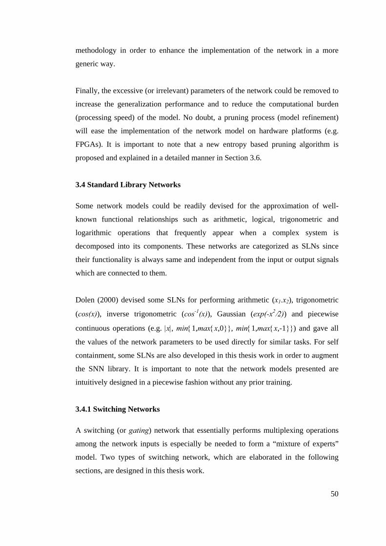
50

methodology in order to enhance the implementation of the network in a more

generic way.

Finally, the excessive (or irrelevant) parameters of the network could be removed to

increase the generalization performance and to reduce the computational burden

(processing speed) of the model. No doubt, a pruning process (model refinement)

will ease the implementation of the network model on hardware platforms (e.g.

FPGAs). It is important to note that a new entropy based pruning algorithm is

proposed and explained in a detailed manner in Section 3.6.

3.4 Standard Library Networks

Some network models could be readily devised for the approximation of well-

known functional relationships such as arithmetic, logical, trigonometric and

logarithmic operations that frequently appear when a complex system is

decomposed into its components. These networks are categorized as SLNs since

their functionality is always same and independent from the input or output signals

which are connected to them.

Dolen (2000) devised some SLNs for performing arithmetic (x1.x2), trigonometric

(cos(x)), inverse trigonometric (cos-1(x)), Gaussian (exp(-x2/2)) and piecewise

continuous operations (e.g. |x|, min{1,max{x,0}}, min{1,max{x,-1}}) and gave all

the values of the network parameters to be used directly for similar tasks. For self

containment, some SLNs are also developed in this thesis work in order to augment

the SNN library. It is important to note that the network models presented are

intuitively designed in a piecewise fashion without any prior training.

3.4.1 Switching Networks

A switching (or gating) network that essentially performs multiplexing operations

among the network inputs is especially be needed to form a “mixture of experts”

model. Two types of switching network, which are elaborated in the following

sections, are designed in this thesis work.

51

3.4.1.1 Switching Network Type 1

In the first type of the switching network, the output is equal to the first input (u1)

when s = 1 while the second argument (u2) passes if s = -1. As illustrated in Fig.

3.4, this network is a two layered feed-forward network that could be expressed as:

( )2 1 1 1y V W u b V u= Ψ + + (3.4a)

1

1 11

0,

0W b

κκ κκκ κ

−

−

−⎡ ⎤ ⎡ ⎤= =⎢ ⎥ ⎢ ⎥

⎣ ⎦⎣ ⎦ (3.4b)

[ ] [ ]1 20 0 ,V Vκ κ κ= − = (3.4c)

where u = [u1 u2 s]T is the input vector; y is the output of the network; Ψ(.) is an

activation (tangent sigmoid) vector function. To transmit the signal through the

activation function without any distortion, the value of κ should be high enough to

scale down input of the neuron (by κ-1) into the linear part of the tangent sigmoid.

Then, the output of the activation function is rescaled with κ to form the original

input signal.

κ

κ

κ−

κ−

κ

κ

κ

1κ −

1κ −

Fig. 3.4 Switching Network Type 1.

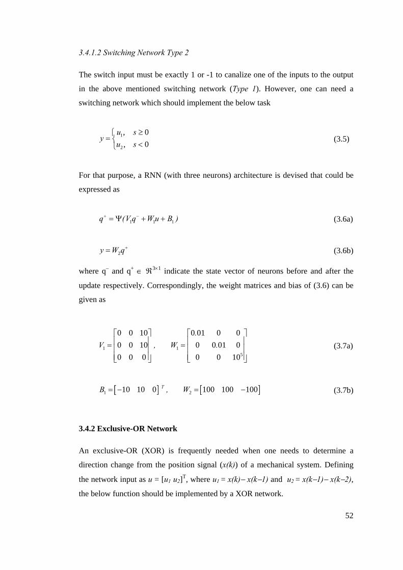
52

3.4.1.2 Switching Network Type 2

The switch input must be exactly 1 or -1 to canalize one of the inputs to the output

in the above mentioned switching network (Type 1). However, one can need a

switching network which should implement the below task

1

2

, 0, 0

u sy

u s≥⎧

= ⎨ <⎩ (3.5)

For that purpose, a RNN (with three neurons) architecture is devised that could be

expressed as

1 1 1q (V q W u B )+ −= Ψ + + (3.6a)

2y W q+= (3.6b)

where q– and q+ ∈ ℜ3×1 indicate the state vector of neurons before and after the

update respectively. Correspondingly, the weight matrices and bias of (3.6) can be

given as

1 15

0 0 10 0 01 0 00 0 10 0 0 01 00 0 0 0 0 10

.V , W .

⎡ ⎤ ⎡ ⎤⎢ ⎥ ⎢ ⎥= =⎢ ⎥ ⎢ ⎥⎢ ⎥ ⎢ ⎥⎣ ⎦ ⎣ ⎦

(3.7a)

[ ] [ ]1 210 10 0 100 100 100TB , W= − = − (3.7b)

3.4.2 Exclusive-OR Network

An exclusive-OR (XOR) is frequently needed when one needs to determine a

direction change from the position signal (x(k)) of a mechanical system. Defining

the network input as u = [u1 u2]T, where u1 = x(k)− x(k−1) and u2 = x(k−1)− x(k−2),

the below function should be implemented by a XOR network.

53

( ) ( )1 21,1,

⎧− == ⎨⎩

sgn u sgn uy

else (3.8)

The analytical expression of the XOR network could be written as

3 2 1 2 3( ( ) )y W W W u B B= Ψ Ψ + + (3.9a)

where the weight matrices and biases become

11 2 2 2

0, ,

0K K K K

W W BK K K K

− −⎡ ⎤ ⎡ ⎤ ⎡ ⎤= = =⎢ ⎥ ⎢ ⎥ ⎢ ⎥−⎣ ⎦ ⎣ ⎦ ⎣ ⎦

(3.9b)

[ ]3 31 1 , 1W B= − = (3.9c)

In (3.9b), K refers to a large gain (typically 105) in order to drive the tangent

sigmoid functions into the saturation.

3.5 Standard Network Architectures

Although some widely known black-box model architectures are given in Section

3.2, they may not be an appropriate model structures when devising a network

model for a discrete-time sub-system at the second step of the proposed SNN

methodology. Covering all the black-box models, other network architecture

templates are given in Fig. 3.5. As could be seen, all the standard network

architectures are comprised from the basic operations of delay elements (TDL),

feed-forward multi-layered networks having tangent sigmoid neurons (illustrated as

f(.) and g(.)), and summation blocks. Using the multi-layered networks in cascade

and feedback configurations with the TDL inputs to such models, arbitrary discrete-

time nonlinear sub-systems could be modeled efficiently. Table 3.2 indicates which

template should be used for which type of discrete-time sub-system.

54

Tβ

Tβ

Tα

Fig. 3.5 Standard network templates.

55

Table 3.2 Discrete-time systems and their corresponding network templates.

Type Discrete-time System Model

1 y(k+1) = f[x(k), x(k-1), x(k-2),…]

2 y(k+1) = f[y(k), y(k-1),..,x(k), x(k-1), x(k-2),…]

3 y(k+1) = g[y(k), y(k-1), y(k-2),…] + f[x(k), x(k-1), x(k-2),…]

4 y(k+1) = g[y(k), y(k-1), y(k-2),…] + ( )0

ii

x k iβ=

−∑

5 y(k+1) = ( )0

ii

y k iα=

−∑ + f[x(k), x(k-1), x(k-2),…]

6 y(k+1) = g{y(k), y(k-1), y(k-2),…, f[x(k), x(k-1), x(k-2),…]}

7 y(k+1) = g{ y(k), y(k-1), y(k-2),…, f[x(k), x(k-1), x(k-2),… y(k), y(k-1),

y(k-2),…]}

8 y(k+1) = g{ y(k), y(k-1), y(k-2),…, f[x(k), x(k-1), x(k-2),… y(k), y(k-1),

y(k-2),…]} + ( )0

ii

x k iβ=

−∑

3.6 Entropy Based Pruning Algorithm

Although there are a lot of different pruning methods as could be seen from the

literature survey in Chapter 2, an entropy based pruning algorithm, which is mainly

adapted from the smallest variance pruning (SVP) method, is utilized whenever a

pruning operation will be needed for a devised neural network. In SVP, the units,

which have approximately constant (or smallest variance) outputs across the

training set, are deleted. The primary problem with this simple and effective

pruning algorithm is that the inessential units must be identified manually and there

is not a built-in mechanism which automates the procedure for large and complex

networks (Guan and Chen, 2005). In this thesis work, this problem is solved

through calculating the uncertainty of each hidden neuron output via entropy (H)

approach.

Entropy is defined as the uncertainty of a single random variable in statistical

mechanics. On the other hand, information theory uses the entropy as a measure of

56

information. In fact, entropy is a function of a probability (i.e. H(p)); therefore, it

does not rely on the apparent value of the random variables. It is obvious that if an

event with a low probability is happened, one will get the most information (i.e.

information is inversely related to the probability of occurrence). Therefore, entropy

is frequently used to measure the uncertainty, or to get the information content of an

interested variable.

Now, an entropy function H(p) will be constructed based on the three properties

about entropy and probability laws as

1. H(p) ≥ 0 (entropy always increases)

2. H(p1.p2) = H(p1) + H(p2) (independent events are additive)

3. H(p) is a continuous function of p (0 ≤ p ≤ 1).

From second property, some manipulations could be written as below

( ) ( )nH p n H p= (3.10a)

1/,n np y p y= = (3.10b)

( ) ( )1/ nH y n H y= (3.10c)

( ) ( )/m n mH y H yn

= (3.10d)

From the above manipulations, it is seen that an entropy function obeys the

logarithmic function rules and could be written for some base of the log system for

any constant k as below

( ) ( )logH p k p= (3.11)

From first property, k must be non-positive and could be chosen as -1. Moreover,

considering pi as the probability of getting the information H(pi), one will get all the

information H(p) on the average with using the third property as

57

( )1

1logii i

H p pp=

⎡ ⎤⎛ ⎞= ⎢ ⎥⎜ ⎟

⎢ ⎥⎝ ⎠⎣ ⎦∑ (3.12)

It does not matter which base of the log system is used. If the base is chosen as 2,

the resulting units of information will a bit (binary digit). Furthermore, if the used

base is e, then the unit of information is called a nat (Hamming, 1986). For the idea

of entropy, let’s consider an example in which the output variable is either 1 or 0. It

is obvious that if the probability of the output being 1 is p, then the probability of

being 0 will be 1-p. Based on these assumptions, the entropy function of this event

(in bit units) could be written as

( ) ( )2 21 11

1H p p log p log

p p⎛ ⎞ ⎛ ⎞

= + −⎜ ⎟ ⎜ ⎟−⎝ ⎠ ⎝ ⎠ (3.13)

The graph of this entropy function is given in Fig. 3.6. It is seen that H(p) gets its

maximum value (1 bit) when p = 1/2 (uncertainty is maximum). On the other hand,

it is 0 when p equals 0 or 1, meaning that the output variable is not random but

constant (no uncertainty).

0 0.1 0.2 0.3 0.4 0.5 0.6 0.7 0.8 0.9 10

0.1

0.2

0.3

0.4

0.5

0.6

0.7

0.8

0.9

1

p

H(p

)

Fig 3.6 Entropy functions for two probabilities.

58

Considering that the output of a hidden layer neuron is an information source, one

can use the entropy to evaluate the uncertainty of a neuron. The flowchart of the

entropy based pruning algorithm is shown in Fig.3.7. In the proposed pruning

method, entropy is defined as the weighted average of the natural logarithms of the

reciprocals of the probability density function (pdf) of the neuron output in its

whole working range (-1 ≤ working range ≤ +1 for tangent sigmoid neurons) and

calculated as below

( )1 1

1log logi e i e iii i

H pdf pdf pdfpdf= =

⎡ ⎤⎛ ⎞= = − ⎡ ⎤⎜ ⎟ ⎣ ⎦⎢ ⎥⎝ ⎠⎣ ⎦∑ ∑ (3.14)

Consequently, neurons with a small entropy value (or uncertainty) could be

removed from the network in an automated fashion. But, the mean output of the

removed neurons should be added as the bias weights of the neurons in connection

with the removed one in order to keep the network’s performance (almost)

unchanged. Following that, the pruned network should be retrained for fine tuning

of the remaining parameters. After the retraining operation, if the network could not

reach the predetermined error threshold value, one should revert to the previous

network architecture (undo last pruning operation) and terminate the pruning

process. In the next sub-sections, two benchmark systems are utilized to show the

efficiency of the proposed algorithm for a pruning process. The first system is taken

from Lazar and Pastravanu (2002) and the second system is adapted from Narendra

and Parthasarathy (1990).

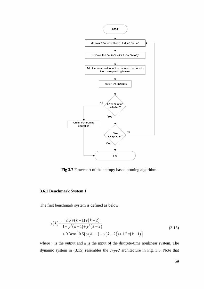
59

Fig 3.7 Flowchart of the entropy based pruning algorithm.

3.6.1 Benchmark System 1

The first benchmark system is defined as below

( ) ( ) ( )( ) ( )

( ) ( )( ) ( )

2 2

2.5 1 21 1 2

0.3cos 0.5 1 2 1.2 1

y k y ky k

y k y k

y k y k u k

− −=

+ − + −

⎡ ⎤+ − + − + −⎣ ⎦

(3.15)

where y is the output and u is the input of the discrete-time nonlinear system. The

dynamic system in (3.15) resembles the Type2 architecture in Fig. 3.5. Note that

60

training such a recurrent model with randomly initialized parameters is known to be

very difficult. For that reason, first a NARX type model (with ten neurons in its first

hidden layer) is trained. Following that, its parameters are used as the initial

conditions of the Type2 structure (NOE type black-box model). Fig. 3.8 shows the

applied input signal to the plant and the target response that are used in the training

session.

Consequently, a NOE model is trained by taking the initial conditions (weights) of

the parameters from the NARX model. Table 3.3 shows the training performance of

the network. As can be seen in Fig. 3.9, some instability and divergence problems

are encountered while validating the NOE#1. As previously suggested, the number

of the hidden layer neurons are not increased gradually but increased extremely

(from 10 to 30) not to make a lot of trials. In this way, a NARX model having 30

neurons in the first layer is trained first and; then, again a NOE model is devised by

taking the initial conditions of the parameters from the NARX. At the end, a well

trained recurrent network model (NOE#2) but having an excessive number of

neurons in its hidden layer is achieved as could be seen from Table 3.3. Although

this model passes the model validation test successfully, one may demand to finish

the identification process with a network model having a less number of neurons.

0 50 100 150 200 250 300 350 400 450 500

-1

-0.8

-0.6

-0.4

-0.2

0

0.2

0.4

0.6

0.8

1

Samples

a) Input signal applied to the plant.

61

0 50 100 150 200 250 300 350 400 450 500-1

-0.5

0

0.5

1

1.5

2

Samples

b) Target response.

Fig 3.8 Training scenario used for benchmark system 1.

Table 3.3 Black-box networks for benchmark system 1*.

Model NARX#1 NARX#2 NOE#1 NOE#2

Input(s) u(k-1), y(k-1), y(k-2) u(k-1)

Output y(k)

Training data 501 Samples

1st layer neurons 10 30 10 30

Training time (seconds) 57 98 57 63

Epochs 5000 50

Mean-square training error

1.11×10-6 6.43×10-10 1.38×10-6 7.4×10-10

Activation Function Tangent (Bipolar) Sigmoid

[*] Linear activation functions are utilized at their output layers.

62

0 50 100 150 200 250-2

-1.5

-1

-0.5

0

0.5

1

1.5

2

Samples

NOE#1 responseplant response

Fig 3.9 Validation performance of NOE#1. For a pruning operation, probability density functions of the hidden layer neurons in

NOE#2 are calculated first, and then, (3.14) is used to calculate the entropy value of

the each neuron separately. As could be seen from Fig. 3.10, neurons indexed with

16, 28 and 30 have an entropy value closer to zero, meaning that their activation

function outputs are not changing too much during the training process. After

pruning these three neurons from NOE#2, another network named as NOE#3 is

created, and then, trained for fine tuning of the network parameters. Again, the

entropy of the neurons in NOE#3 is recalculated and given in Fig 3.11. Now, the

neurons indexed with 11, 21 and 25 are removed and a network called NOE#4 is

formed after this operation.

One more iteration is carried out via looking to the entropy diagram of NOE#4,

given in Fig. 3.12, in which the neurons indexed with 13 and 21 are pruned and a

network called NOE#5 is created at last. From that point on, it is seen that no further

neuron could be pruned and the rest network parameters could be trained in an

effective way. Eventually, after 3 iterations, the number of the neurons is decreased

from 30 to 22 by using this simple and effective pruning technique. Fig. 3.13 shows

the validation performances of the NOE#2 and NOE#5. It is seen that the NOE#2

was easily pruned without deteriorating its modeling performance.

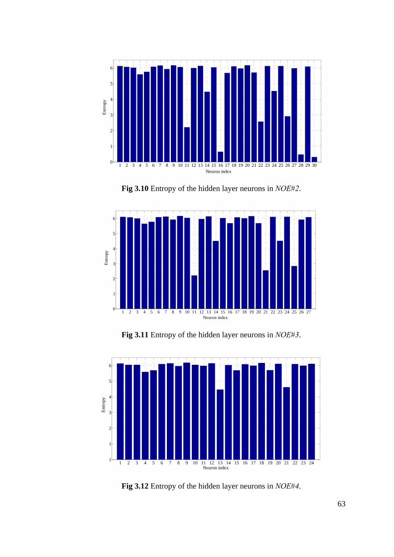
63

1 2 3 4 5 6 7 8 9 10 11 12 13 14 15 16 17 18 19 20 21 22 23 24 25 26 27 28 29 300

1

2

3

4

5

6

Neuron index

Entro

py

Fig 3.10 Entropy of the hidden layer neurons in NOE#2.

1 2 3 4 5 6 7 8 9 10 11 12 13 14 15 16 17 18 19 20 21 22 23 24 25 26 270

1

2

3

4

5

6

Neuron index

Entro

py


1 2 3 4 5 6 7 8 9 10 11 12 13 14 15 16 17 18 19 20 21 22 23 241

1

2

3

4

5

6

Neuron index

Entro

py


64

0 50 100 150 200 250-2.5

-2

-1.5

-1

-0.5

0

0.5

1

1.5

2

Samples

plant responseNOE 30NOE 22

236 238 240 242 244 246

-2

-1.5

-1

-0.5

0

0.5

1

1.5

Fig 3.13 Validation performance of NOE#2 and NOE#5.

3.6.2 Benchmark System 2

In the second benchmark example, the system is assumed to be of the form

( ) ( ) ( ) ( ) ( ) ( ) ( )( ) ( )2 2

1 2 1 2 11

1 2 1y k y k y k u k y k u k

y ky k y k

− − − − − +⎡ ⎤⎣ ⎦+ =+ − + −

(3.16)

where y is the output and u is the input of the discrete-time nonlinear system. In the

identification process, as used by Narendra and Parthasarathy (1990), a three-

layered NOE-type network model structure is chosen. The number of tangent

sigmoid neurons is 20 and 10 in the first and second layers, respectively while one

linear neuron is used in the output layer. As mentioned earlier, this network model

is trained first in a feed-forward manner (i.e. a NARX model is created), meaning

that the measured output values are used in the regression vector. Then, using the

values of estimated parameter of the NARX model as the initial conditions of the

NOE parameters, a recurrent learning is performed. A uniformly distributed random

input signal is used in the training session as depicted in Fig. 3.14.a and the

corresponding output of the plant is illustrated in Fig. 3.14.b.

65

0 100 200 300 400 500 600 700 800 900 1000-1

-0.8

-0.6

-0.4

-0.2

0

0.2

0.4

0.6

0.8

1

Samples

u(k)

a) Input signal applied to the plant.

0 100 200 300 400 500 600 700 800 900 1000-1

-0.8

-0.6

-0.4

-0.2

0

0.2

0.4

0.6

0.8

1

Samples

y(k+

1)

b) Target response.

Fig 3.14 Training signals used for benchmark system 2.

Next, the entropy value of the each neuron in the hidden layers of the network is

calculated. Fig. 3.15 presents the entropy diagrams for the first- and second hidden

layers of the recurrent neural network (NOE-type). The entire procedure given in

the flowchart of the entropy based pruning algorithm (see Fig. 3.7) is followed step-

by-step in 3 iterations. The neuron indexed with 2 in first hidden layer and the

neuron indexed with 10 in the second hidden layer is purged in the first iteration. In

the second iteration, only the neuron indexed with 1 is removed from the first layer.

66

It is seen that no further neuron could be pruned from the second layer after pruning

one neuron from it at the first iteration. Lastly, the indexed neurons with 11, 12 and

17 in Fig. 3.15.a are purged in the third iteration. Table 3.4 shows the training

performances of the devised network models.

1 2 3 4 5 6 7 8 9 10 11 12 13 14 15 16 17 18 19 200

1

2

3

4

5

6

7

Neuron index

Entro

py

a) Entropy diagram of the first hidden layer.

1 2 3 4 5 6 7 8 9 100

1

2

3

4

5

6

7

Neuron index

Entro

py

b) Entropy diagram of the second hidden layer.

Fig 3.15 Entropy diagrams of the hidden layer neurons in NOE.

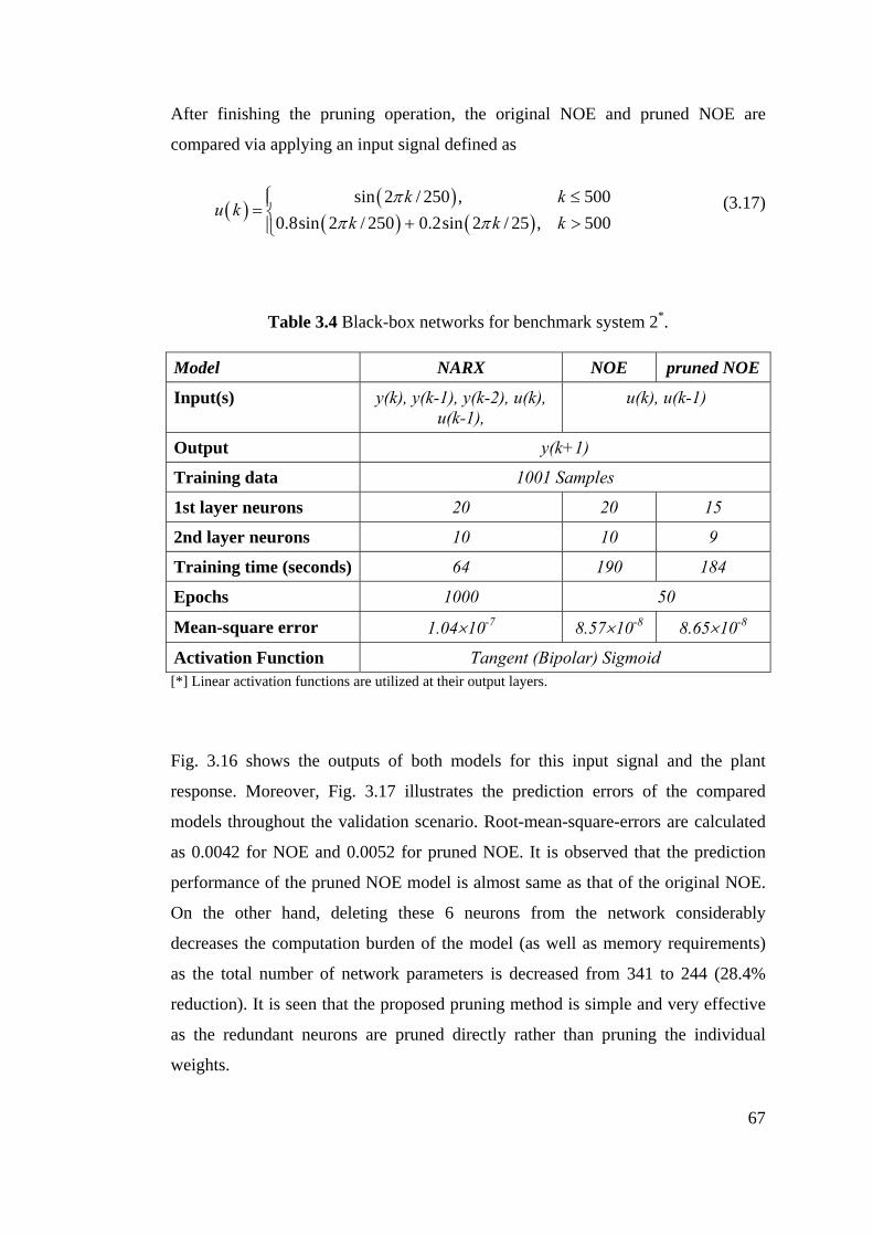
67

After finishing the pruning operation, the original NOE and pruned NOE are

compared via applying an input signal defined as

( ) ( )( ) ( )

sin 2 / 250 , 5000.8sin 2 / 250 0.2sin 2 / 25 , 500

k ku k

k k kπ

π π≤⎧⎪= ⎨ + >⎪⎩

(3.17)

Table 3.4 Black-box networks for benchmark system 2*.

Model NARX NOE pruned NOE

Input(s) y(k), y(k-1), y(k-2), u(k), u(k-1),

u(k), u(k-1)

Output y(k+1)

Training data 1001 Samples

1st layer neurons 20 20 15

2nd layer neurons 10 10 9

Training time (seconds) 64 190 184

Epochs 1000 50

Mean-square error 1.04×10-7 8.57×10-8 8.65×10-8

Activation Function Tangent (Bipolar) Sigmoid [*] Linear activation functions are utilized at their output layers. Fig. 3.16 shows the outputs of both models for this input signal and the plant

response. Moreover, Fig. 3.17 illustrates the prediction errors of the compared

models throughout the validation scenario. Root-mean-square-errors are calculated

as 0.0042 for NOE and 0.0052 for pruned NOE. It is observed that the prediction

performance of the pruned NOE model is almost same as that of the original NOE.

On the other hand, deleting these 6 neurons from the network considerably

decreases the computation burden of the model (as well as memory requirements)

as the total number of network parameters is decreased from 341 to 244 (28.4%

reduction). It is seen that the proposed pruning method is simple and very effective

as the redundant neurons are pruned directly rather than pruning the individual

weights.

68

0 100 200 300 400 500 600 700 800-1

-0.8

-0.6

-0.4

-0.2

0

0.2

0.4

0.6

Samples

plant responseNOEpruned NOE

Fig 3.16 Validation performances of NOE and pruned NOE.

0 100 200 300 400 500 600 700 800-0.02

-0.015

-0.01

-0.005

0

0.005

0.01

0.015

0.02

0.025

0.03

Samples

Pred

ictio

n Er

ror

NOEpruned NOE

Fig 3.17 Prediction errors of NOE and pruned NOE.

3.7 Closure

This chapter has presented a modeling and identification procedure for nonlinear

dynamic systems using ANNs. First, black-box modeling procedure has been

explained. Every step of this identification process (the data preparation, model

69

structure selection, parameter estimation and model validation) was elaborated in a

detailed manner. The procedure was known to be very time-consuming since one

need to consider a number of issues (i.e. different model structures, different

number of neurons in the chosen model architecture and different initial conditions

while starting the training of the parameters). Hence, a general methodology to

model nonlinear dynamic systems using SNNs was proposed. Several stages of the

proposed methodology (division, unification, and pruning) were all explained in a

step wise procedure. Furthermore, some standard library networks were developed

and an iterative entropy based pruning algorithm was also proposed, which is one of

the contributions of the thesis work.

70

CHAPTER 4

POSITION ESTIMATION FOR TIMING BELT DRIVES

OF PRECISION MACHINERY 4.1 Introduction

Precision positioning systems are used in a wide variety of applications in

manufacturing-, automation-, semiconductor-, and biomedical industries (Kulkarni

and El-Sharkawi, 2001). Almost all of these systems use a rotary actuator (such as

a brushless DC motor) where its angular motion is converted into translation by

mechanical power transmission elements like belts, chains, rack-and-pinion,

traction (friction) drives, and ball/lead-screws. The drive system is usually selected

by considering various issues including positioning accuracy/repeatability sought,

travel span, maximum speed, load capacity, and cost. At present, high precision

systems (requiring repeatability less than 100 microns) frequently employ rigid (or

stiff) elements like ball-screws owing to the fact that comparable performance

cannot be achieved with elastic transmission elements like timing belts, cable, chain

etc. For the systems with elastic elements, positioning accuracy is obtained through

direct load position measurement devices (like linear encoders) at the increased

hardware cost (Zhao and Cai, 1996). Furthermore, elastic elements in such

arrangements is known to introduce nonlinearities (backlash, spatial variations in

stiffness, friction, etc.) to the system which may in turn lead to limit cycles in the

controlled system (Li and Rehani, 1996). This drawback oftentimes calls for more

elaborate control- and estimation schemes that can compensate for such effects to

improve system’s stability and performance by incorporating advanced system

models (Hace et al., 2005; Zaki et al. 2008). Consequently, the main motivation of

71

this work is to propose a feasible estimation scheme for timing-belt drives (TBDs)

that utilize the information emanating from a low-cost sensor on the driver side

(pulley). Hence, the position of the carriage driven through a timing belt could be

estimated for cost-sensitive computer numerical control (CNC) applications.

To predict the transmission error of TBDs, detailed dynamic (and kinematic)

models must be taken into consideration. Surprisingly, TBDs are somewhat

neglected in the technical literature and thus (unlike gears) their dynamic attributes

have not been fully investigated. In fact, the transmission error of a TBD depends

on many different factors such as belt-pinion material pair, form errors in elements,

eccentricity of the pinion, radial/axial vibrations of the belt, belt-tension, interface

temperature, etc. Hence, the functional dependency between the actual position of

the carriage and that of the pinion is quite complicated. On the other hand, NNs,

which are capable of learning complex mappings, are the most suitable tools to

approximate these error patterns. Unfortunately, large number of cited

nonlinearities makes it quite difficult for a single (recurrent) NN topology to learn

the complete task satisfactorily due to weak initial assumptions associated with the

NN models. That is, the learning goal cannot be attained through a properly-sized

NN topology within a reasonable time frame. As an alternative, a structured neural

network topology is also proposed in this chapter for the solution of this challenging

estimation problem.

In the presented work, the TBD under study is divided into its components

employing the physical models. Unlike classical SNN approach, the inputs of the

presented neural networks are speculated via sketchy guidance of the relevant

processes under investigation. Hence, the resulting neural networks are trained to

explore their sub-domains via extensive training data sets. As a consequence, the

overall network is expected to go beyond the physical model at hand so as to

capture unaccounted system attributes.

The organization of this Chapter 4 is as follows: After the introduction part, Section

4.2 elaborates the generic TBD considered in this work. Then, Section 4.3

72

introduces the experimental setup along with a number of accompanying

evaluations to investigate the transmission characteristics of a TBD. Based on the

information collected, various neural network topologies are proposed in Section

4.4 and Section 4.5. Next, Section 4.6 illustrates the estimation performance of the

proposed model. Finally, the key points of the work are discussed in detail in

Section 4.7.

4.2 Timing Belt Drive

Fig. 4.1 illustrates the generic TBD considered in this work. There exist two

distinct modes of operations in such mechanisms:

i. Teeth of driving pinion and the (driven) timing belt are fully engaged and thus

the resulting dynamic system acts like (lower order) lumped system;

ii. Teeth are disengaged due to backlash but (unlike gears) the torque is still

transmitted through the friction coupling between these elements.

Fig. 4.1 A generic timing (synchronous) belt drive system.

Kilic (2007) offers a dynamic model that takes into account the properties of these

regimes. The presented model reveals hysteresis-type nonlinearity. In fact, there

exist a significant number of research efforts on systems with hysteresis. The most

popular hysteresis model (which is a carry-over from the studies on electro-

magnetism and ferromagnetic materials) is the Preisach model (Mayergoyz, 1991).

73

This domain-independent modeling technique has well-defined features (such as its

ability to model complex hysteresis types, identification algorithm, and

implementation) which make it a suitable candidate for control applications.

Unfortunately, the Preisach model is not particularly adequate to model the

hysteretic effects of TBDs since such dynamic systems evidently incorporate both

local- and global memory which is a condition violating the congruent minor-loop

property of basic Preisach model.

Note that devising general-purpose estimator/observer (with nonlinear properties),

which directly embodies such complex dynamic models, is quite challenging due to

obvious implementation difficulties such as numerical instability, divergence, high

real-time computational cost, etc. Hence, this study proposes a feasible “gray-box”

approach for the estimation problem at hand.

4.3 Experimental Studies

To develop a general-purpose estimator, the transmission error of a TBD (not

subjected to any external load or any other change in its operation parameters)

should be repeatable (i.e. deterministic). Thus, a test setup is designed to test the

validity of this basic assumption first. Remaining of this section introduces the test

setup and the experimental procedure implemented on this setup.

4.3.1 Test Setup

Figs.4. 2 and 4.3 show the experimental setup and its corresponding schematic.

Here, the preload of TBD can be adjusted by changing the location of the free

wheel. Note that the belt preload is not measured but indirectly estimated by

considering the nominal stiffness of the timing belt. A high resolution linear scale

(LS) is integrated into this setup for modeling and verification purposes. This

experimental setup is used to simulate several scenarios where the velocity and

acceleration profiles of the carriage are accurately controlled to investigate the slip

dynamics of the mechanism.

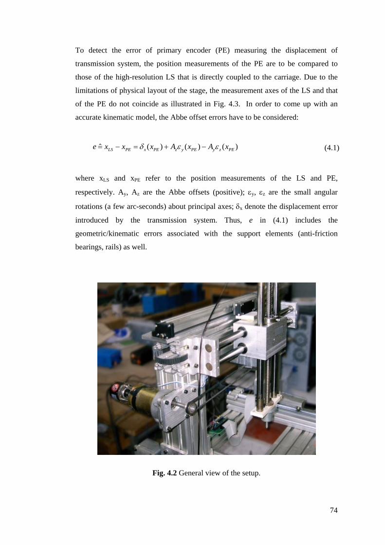
74

To detect the error of primary encoder (PE) measuring the displacement of

transmission system, the position measurements of the PE are to be compared to

those of the high-resolution LS that is directly coupled to the carriage. Due to the

limitations of physical layout of the stage, the measurement axes of the LS and that

of the PE do not coincide as illustrated in Fig. 4.3. In order to come up with an

accurate kinematic model, the Abbe offset errors have to be considered:

( ) ( ) ( )ˆ LS PE x PE z y PE y z PEe x x x A x A xδ ε ε= − = + − (4.1)

where xLS and xPE refer to the position measurements of the LS and PE,

respectively. Ay, Az are the Abbe offsets (positive); εy, εz are the small angular

rotations (a few arc-seconds) about principal axes; δx denote the displacement error

introduced by the transmission system. Thus, e in (4.1) includes the

geometric/kinematic errors associated with the support elements (anti-friction

bearings, rails) as well.

Fig. 4.2 General view of the setup.

75

Fig. 4.3 Schematic of experimental setup.

4.3.2 Experiments

In this work, several tests are conducted to show the repeatability of the motion

which is a prerequisite to devise reliable reference models. In all tests, the motor’s

velocity is accurately controlled along a trapezoidal path as shown in Figure 4.4.

This velocity pattern corresponds to a carriage round-trip along a 300mm path.

Thereafter, the carriage is driven with constant velocity (assumed to be in steady-

state, i.e., the acceleration / deceleration of the system is negligible) along its full

span, the positioning error patterns (e) for twelve different (overlaid) trajectories are

plotted in Fig. 4.5.a. Fig. 4.5.b shows the zoom window in Fig. 4.5.a. Note that the

waveform (with low-frequency content) in Fig. 4.5.a (shown as dashed red line) is

the (low-pass filtered) positioning error and is employed as a reference for the

major hysteresis band. As can be seen from Fig. 4.5.b, the positioning errors are

quite repeatable (systematic) which in turn encourages the development of

advanced estimator models. Despite its high repeatability, the tooth-passing

frequency component is deliberately neglected in this work owing to the fact that

76

this component is mainly a function of form errors associated with the timing belt

and pinion. Hence, it highly depends on starting position (i.e. initial conditions) of

the mechanism.

0 2 4 6 8 10 12

-60

-40

-20

0

20

40

60

Time [sec]

Velo

city

[mm

/s]

linear scalerotary encoder

Fig. 4.4 Velocity profile of the carriage measured from the LS and the PE.

0 50 100 150 200 250 300

-0.2

-0.1

0

0.1

0.2

0.3

Position [mm]

Erro

r [m

m]

errorfiltered error

zoom window

a) Error trajectories.

77

175 180 185 190 195 200 205 210 215 220-0.11

-0.1

-0.09

-0.08

-0.07

-0.06

-0.05

-0.04

-0.03

-0.02

Position [mm]

Err

or [m

m]

b) Exploded view.

Fig. 4.5 Position error trajectories of 12 different cases.

Close examination of the error patterns in Fig. 4.5 reveals critical points about the

attributes of the system under investigation:

• Hysteresis band, which is roughly 0.3 mm for the test cases, is apparently a

consequence of the backlash between the timing belt and the driving pinion

(pulley). It is obvious that an increase or decrease in the belt tension will create

contraction or expansion in the length of the timing belt which in turn modifies

dead-zone characteristic of meshing teeth pairs (Kulkarni, El-Sharkawi, 2001).

Note that in all the experiments the operating conditions (carriage mass,

ambient temperature) along with belt preload are kept constant.

• As mentioned earlier, unless Ay and Az are zero [see (4.1)], the Abbe offset

errors manifest themselves as the waveforms on the upper and lower

boundaries. Hence, mechanical manipulations on the bearing elements usually

impress a different texture on these bounds. That is, the use of different linear

bearing elements (with different geometric form errors, running parallelism and

straightness errors) and/or corresponding assembly errors creating geometric

78

congruence between interfacing elements might alter the spatial attributes of

the major hysteresis band.

• A fundamental harmonic component (with a magnitude of 15 microns)

superimposed onto the band is at the tooth-passing (meshing) frequency (i.e.

carriage velocity ÷ pitch) of the timing belt and thus the observed variations

could be mainly attributed to the effect of belt-climbing as well as the form

errors of the belt (Kagotani et al., 2001).

Harmonics injected by the two-stage gearbox of the motor appear to be quite

negligible while the transition in the backlash zone (of which has bandwidth of 0.12

mm) is extremely fast (< 1 ms) when a change in the direction of motion is

observed.

The next set of experiments focuses on the effect of velocity and inertial forces on

the transmission error. As can be seen from Fig. 4.6, the dramatic changes at the

steady-state velocity have some influences on the nature of the nonlinear

relationship. Moreover, the effect of inertial forces is investigated by modifying the

acceleration and deceleration profile of the controlled motor such that the sliding

motion inside the hysteresis band is induced under the action of these inertial forces.

The inertial forces do not have a considerable effect on the closing distances as

illustrated in Fig. 4.6. To identify the reversal path inside the hysteresis band, the

TBD mechanism is programmed to reverse its course at every 25 mm and go back

to its starting point. This procedure is repeated in both directions (forward and

backward). Similarly, the collected (and low-pass filtered) data shown in Fig. 4.7

reveal the closing distances when the direction of motion is reversed at the above

mentioned intervals. It is obvious that when the direction of travel is reversed, the

power transmitting teeth disengage and micro-slip under external excitation comes

into play. As a consequence, the belt slowly slides until the different set of teeth

pairs engage into transmission. Unfortunately, developing dynamic models that

explain the observed phenomena satisfactorily is known to be quite challenging and

is an active research field in tribology (Astrom and Canudas-De-Wit, 2008).

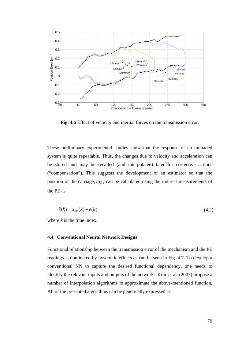
79

-50 0 50 100 150 200 250 300 350-0.3

-0.2

-0.1

0

0.1

0.2

0.3

0.4

0.5

Position of the Carriage [mm]

Pos

ition

Erro

r [m

m]

108mm/s254mm/s2

27mm/s2326mm/s2216mm/s2

60mm/s80mm/s

40mm/s25mm/s

Fig. 4.6 Effect of velocity and inertial forces on the transmission error.

These preliminary experimental studies show that the response of an unloaded

system is quite repeatable. Thus, the changes due to velocity and acceleration can

be stored and may be recalled (and interpolated) later for corrective actions

(“compensation”). This suggests the development of an estimator so that the

position of the carriage, )(ˆ kx , can be calculated using the indirect measurements of

the PE as

ˆ( ) ( ) ( )PEx k x k e k= + (4.2)

where k is the time index.

4.4 Conventional Neural Network Designs

Functional relationship between the transmission error of the mechanism and the PE

readings is dominated by hysteretic effects as can be seen in Fig. 4.7. To develop a

conventional NN to capture the desired functional dependency, one needs to

identify the relevant inputs and outputs of the network. Kilic et al. (2007) propose a

number of interpolation algorithms to approximate the above-mentioned function.

All of the presented algorithms can be generically expressed as

80

( ) ( ( ), ( 1), ( 2), ( ), ( ))PE PE PE PEe k f x k x k x k x k d e k d= − − − − (4.3)

where xPE(k), xPE(k-1), xPE(k-2) refer to the history of the PE readings while d (a

time-variant positive integer) denotes the time index when the direction change

takes place. Here, f:ℜ5→ℜ represents a Borel measurable function. A RNN can

theoretically capture the desired mapping when all necessary states are presented to

the network at a particular instant (Seidl and Lorenz, 1991).

Fig. 4.7 Position errors on motion reversals at various locations.

In fact, there exists an extensive literature on modeling/identification of hysteretic

systems using ANNs. Previous studies deal with the hysteresis-type problems using

the outputs of the elementary hysteresis operators of the Preisach model as inputs to

the designed FNNs (Zhang and Tan, 2010). For example, Zhao and Tan (2008)

propose a hysteretic operator that was based on the classical Preisach model to

construct an expanded input space of the hysteresis. Moreover, there are some

recent studies which design hysteresis-type ANN models by changing the activation

81

function of the neurons whose characteristic is hysteretic (Lien et al., 2010; Deng

and Tan, 2008).

Within the framework of transmission error estimation, several (supervised) RNN

topologies such as Elman-type RNNs, NOE and fully-recurrent neural network

(FRNN) are considered to approximate the nonlinear relationship. It is well known

that the Elman-type networks are based on FNNs except that they have feedback

connections from hidden layer units to the context units. In NOE, the output of the

second layer is directly connected to the first hidden layer as input. Moreover, all

the layers have feedback connections to the other layers (including self-feedback) in

FRNN. The major assumption here is that the output feedback and the internal

feedback connections of these ANNs are sufficient to form a relevant memory

model (i.e. long-term) implicitly to capture the relationship in (4.3).

The training results of the various RNN models using the input signals in (4.3) are

shown in Table 4.1. As could be seen, the Elman-type RNN (with 50 neurons in its

hidden layer), whose training performance is presented in Fig.4.8, has the smallest

training error. Unfortunately, this network’s generalization performances on some

arbitrary motion scenarios (which will be elaborated in Section 4.7) are

unsatisfactory as could be seen from Fig. 4.9. When the number of hidden-layer

neurons of the network is increased, the training error reaches to an acceptable level

(about 15 μm) after a long training session on a high-end PC (with Intel Core i5

processor and a SDRAM of 4GB). However, the Elman-type networks fail in the

validation scenarios due to various reasons including well-known bias/variance

dilemma (German et al., 1992). Furthermore, when gradient-descent based training

methods are utilized, the developed NNs are not guaranteed to converge to a global

minimum (in a vast parameter space) within a reasonable training period. Within

this context of this study, the Elman-network was clearly not able to form a long-

term memory that allows the recall of the nominal position as well as the error

estimate [namely, xPE(k-d) and e(k-d)] when the direction had changed. Therefore,

independent of the network architecture, the obtained results are unacceptable for

estimation and modeling purposes (i.e. modeling error >> 15 μm).

82

0 50 100 150 200 250 300-0.2

-0.1

0

0.1

0.2

0.3

0.4

0.5

Position [mm]

Err

or [m

m]

Training DataElman Network

Fig. 4.8 Training performance of the Elman-type RNN.

0 50 100 150 200 250 300-0.3

-0.2

-0.1

0

0.1

0.2

0.3

0.4

0.5

Position [mm]

Erro

r [m

m]

hysteresis bandRandom Case ScenarioElman Network

Fig. 4.9 Generalization performance of the Elman-type RNN on Scenario 2.

83

Table 4.1 Training results of the Elman-type RNN, NOE, and FRNN *

Inputs x(k), x(k-1), x(k-2)Output Position Error Training Data 1067 Samples Act. Func. Tangent Sigmoid Training Method Levenberg-Marquardt

Architecture Elman-type RNN NNOE FRNN 1st Layer Neurons 10 25 50 10 25 50 10 25 50

Training error in (μm) 23 19 15 34 33 28 27 22 17

Epochs 125 Training time in (min) 7.5 15.5 55 4 5 6 13 26 85


4.5 Structured Neural Network Architecture

Estimation problem at hand can be decomposed into a number of well-defined sub-

problems that are known to be associated with different operating regimes of the

mechanism. Once a NN is devised to capture the characteristics of each regime, the

corresponding networks can be transformed into a single network to represent the

overall dynamics of the system accurately.

Looking at Fig. 4.7, one can directly identify four different operating regimes for

the given mechanism:

1. Mechanism moves in the forward direction (left to right) while the power/torque

transmitting teeth are fully engaged. The carriage follows the lower bound of the

hysteresis band.

2. Mechanism moves in the reverse (backward) direction (right to left) while the

power transmitting teeth are fully engaged. The carriage follows the upper bound

of the hysteresis band.

84

3. Mechanism changes its course towards the forward direction and thus the power

transmitting teeth become disengaged. In this transient regime, the driving torque

is transmitted through the friction coupling between the pinion and the belt.

Depending on the reversal position, a path inside the hysteresis band (indicated

by solid lines) is followed.

4. Mechanism changes its course towards the reverse direction and thus the power

transmitting teeth become disengaged. The driving torque is again transmitted

through the friction coupling between the pinion and the belt. Depending on the

reversal position, a path inside the hysteresis band (indicated by dashed lines) is

followed.

Hence, four different ANNs can be designed to capture/model the mechanism’s

behavior in each region: ANNe+, ANNe

-, ANNd+, ANNd

- where the superscripts + and

– denote the forward- and reverse directions while the subscripts “e” and “d”

indicate the engagement / disengagement status of the power transmitting teeth in

the mechanism. Fig. 4.10 illustrates the SNN incorporating these units. It is critical

to note that the physical parameters of the timing belt (e.g. pitch of the timing belt,

width, length, mass, number of pinion teeth etc.) are not directly utilized in the

overall network. Since each ANN is trained separately, the weights of the overall

SNN is to implicitly encode the relevant physical parameters.

In this configuration, ANNe+and ANNe

- represent the lower- and upper boundaries of

the hysteresis band in Fig. 4.7. Since there is a one-to-one correspondence between

x(k) (carriage position) and e(k) (estimated error), these networks employ x(k) as

input. Similarly, ANNd+and ANNd

- are trained to approximate a family of

trajectories (curves) lying inside the hysteresis band between the upper and lower

boundaries. In other words, these networks are expected to model the “creep”

behavior of the timing-belt beginning from the disengagement of teeth until the

engagement on the other side of the dead-band. Notice that these two networks have

two inputs: i) reversal (starting) point on the boundaries of hysteresis band; ii)

relative (incremental) position with respect to the starting point on the boundary. If

85

direction reversal takes place inside the hysteresis band (i.e. when the torque/force

is transmitted through friction coupling), the correct course of return needs to be

determined. Hence, two different networks (ANNsp+ and ANNsp

-) are specifically

designed to determine “starting point” (of reversal) on the target boundary using the

information available at the turnaround point inside the band.

Δ

Δ

Δ

Δ

Δ

2Φ

1

2

3

4

5

:::::: ( )

previous positionprevious errorprevious directionposition when direction changederror when direction changedunit delay memory

ΦΦΦΦΦΔ

4Φ

5Φ

1Φ

3ΦΔ

Δ

Δ

Fig. 4.10 SNN topology for estimating the position error of the carriage. Notice that when the direction is reversed (in Fig. 4.7), a considerable jump is

observed at the starting point of a traversed path owing to the fact that the built-in

gearbox of the motor used in this study does have a significant gear backlash.

Hence, two ANNs (namely, ANNb+, ANNb

- ) are included to the SNN to calculate

86

the play introduced by this gearbox. Note that ANNd+ and ANNd

- could be trained to

learn this hard-nonlinearity as well. However, when included, the corresponding

approximation error does increase drastically despite the addition of neurons.

Hence, predicting this (easy-to-model) nonlinearity through the use of separate

networks provides a more effective solution.

As a result, eight separate ANNs are connected together to form a “mixture of

experts” via switching (or gating) networks that essentially perform multiplexing

operations among the network outputs. Design of such NNs is discussed in Section

3.5.1. Here, switching networks Type 2 are used for the implementation of the

below task

1

2

, 0, 0

u sy

u s≥⎧

= ⎨ <⎩ (4.4)

The resulting SNN can be viewed as a finite state machine with five states (Φ1 …

Φ5). In this topology, the Switching Network 1 selects the outputs of the relevant

networks depending on the current direction of the carriage (i.e. sgn{x(k) – x(k-

1)}). Moreover, the direction change is detected via the FNN (with 2 hidden layers)

performing logical exclusive-OR (XOR) operation.

Note that if a change in direction is detected, the Switching Network 3 immediately

latches the last position onto the Φ4 state. Similarly, the Switching Network 4

updates the Φ5 state that essentially holds the last error value including the backlash

calculated by ANNb+or ANNb

-.

When the direction is changed inside the hysteresis band (i.e. teeth are disengaged),

the error could be calculated by first adding the backlash value. Then, the resulting

value is used to find the starting point on the hysteresis boundaries using ANNsp+or

ANNsp-. It is critical to note that in the presented SNN architecture, the states must

continuously monitored to switch to the output of “correct” network (i.e. choose the

proper alternative). For instance, the transition from dead-band to its boundary is

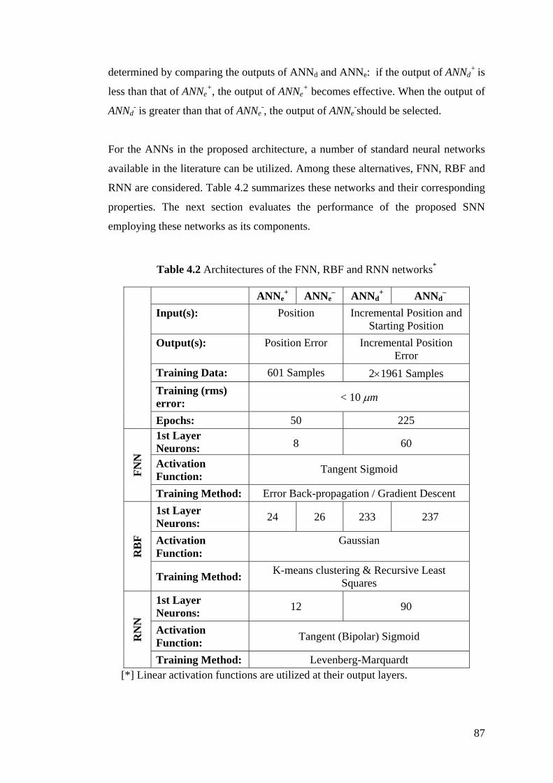
87

determined by comparing the outputs of ANNd and ANNe: if the output of ANNd+ is

less than that of ANNe+, the output of ANNe

+ becomes effective. When the output of

ANNd- is greater than that of ANNe

-, the output of ANNe-should be selected.

For the ANNs in the proposed architecture, a number of standard neural networks

available in the literature can be utilized. Among these alternatives, FNN, RBF and

RNN are considered. Table 4.2 summarizes these networks and their corresponding

properties. The next section evaluates the performance of the proposed SNN

employing these networks as its components.

Table 4.2 Architectures of the FNN, RBF and RNN networks*

ANNe+ ANNe

– ANNd+ ANNd

– Input(s): Position Incremental Position and

Starting Position Output(s): Position Error Incremental Position

Error Training Data: 601 Samples 2×1961 Samples Training (rms) error: < 10 μm

Epochs: 50 225

FNN

1st Layer Neurons: 8 60

Activation Function:

Tangent Sigmoid

Training Method: Error Back-propagation / Gradient Descent

RB

F

1st Layer Neurons: 24 26 233 237

Activation Function:

Gaussian

Training Method: K-means clustering & Recursive Least Squares

RN

N

1st Layer Neurons: 12 90

Activation Function: Tangent (Bipolar) Sigmoid

Training Method: Levenberg-Marquardt [*] Linear activation functions are utilized at their output layers.

88

4.6 Results and Discussions

The estimation capabilities of the proposed SNN are investigated by considering

four arbitrary motion scenarios for the carriage. In each case, the user controls the

velocity and the direction of the carriage manually (at will). The attributes of these

cases are summarized as follows:

• Scenario 1. During its forward motion course, the carriage loops (i.e.

oscillates) around 75, 150, 245 and 295 mms respectively. Similarly, while in

the reverse course the carriage performs these loops at 80, 150 and 230 mms

respectively. Fig. 4.11 shows the trajectory (position and velocity) of the

carriage for this case. The carriage maintains an average velocity of 32 mm/s

on the overall course (when meshing teeth fully engage). While looping, the

pinion- and timing belt teeth disengage at the beginning and then re-engage

when reaching the starting point at the end of the reversal course.

• Scenario 2. This case is similar to the first scenario except that this case

contains longer loops which commence at different points on the course as

could be seen from Fig. 4.12. Note that this case, in which the corresponding

average velocity is 28 mm/s, is selected such that the loop starting points are

distributed out quite evenly throughout the whole travel span.

• Scenario 3. This case, which is illustrated in Fig. 4.13, constitutes five loops

on the forward course and five loops on the backward one. Some of the loops

are cascaded such that the direction is reversed before the meshing teeth fully

engage. For this case, the carriage maintains an average velocity of 24 mm/s

when meshing teeth are fully engaged.

• Scenario 4. This case, which is shown in Fig. 4.14, resembles its predecessor

except the loop starting points. The average velocity maintained on the loops

(i.e. in the region where meshing teeth disengage) is slightly higher than its

counterpart.

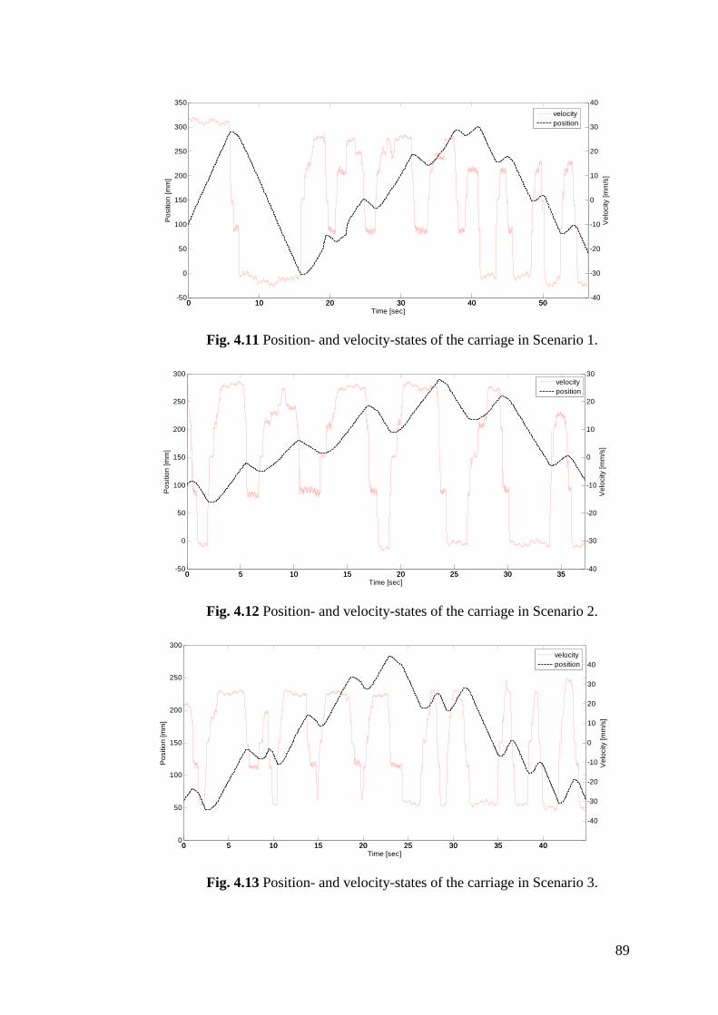
89

0 10 20 30 40 50-50

0

50

100

150

200

250

300

350

Time [sec]

Pos

ition

[mm

]

0 10 20 30 40 50-40

-30

-20

-10

0

10

20

30

40

Vel

ocity

[mm

/s]

velocityposition

Fig. 4.11 Position- and velocity-states of the carriage in Scenario 1.

0 5 10 15 20 25 30 35-50

0

50

100

150

200

250

300

Pos

ition

[mm

]

0 5 10 15 20 25 30 35-40

-30

-20

-10

0

10

20

30

Time [sec]

Vel

ocity

[mm

/s]

velocityposition


0 5 10 15 20 25 30 35 400

50

100

150

200

250

300

Time [sec]

Pos

ition

[mm

]

0 5 10 15 20 25 30 35 40

-40

-30

-20

-10

0

10

20

30

40

Vel

ocity

[mm

/s]

velocityposition


90

0 5 10 15 20 25 30 35 40 450

50

100

150

200

250

300

Time [sec]

Pos

ition

[mm

]

0 5 10 15 20 25 30 35 40 45-75

-50

-25

0

25

50

75

Vel

ocity

[mm

/s]

positionvelocity


Figs. 4.15 to 4.26 demonstrate the estimation performances of the SNN topology on

each case. As for quantitative analysis, the key results [in terms of “estimation

error” characteristics along the traversed trajectory for a SNN incorporating three

different NN types (FNN, RBF, RNN)] are summarized in Table 4.3. Moreover,

Table 4.4 gives the estimation errors on major – and minor hysteresis loops

separately. Note that the major loop is associated with the motion where belt teeth

essentially mesh with pinion teeth. That is, it corresponds to the motion on the

upper- and lower bounds of the hysteresis band. On the other hand, the minor loop

refers to the motion inside the band where the meshing teeth of the mechanism are

fully disengaged and the motion is transmitted by friction coupling. Figs. 4.15,

4.16, and 4.17 show the results of the considered networks for Scenario 1.

Table 4.3 Estimation errors (in μm) for each NN employed in the SNN.

Scenario: 1 2 3 4

FNN

Max 145.2 116.1 92.5 132.6 Min -133.6 -92.2 -149.3 -127.2 RMS 24.1 25.4 30.1 26.8

RB

F Max 101.1 113.4 102.3 129.5 Min -169.2 -85 -192.8 -136.7 RMS 25.9 25.5 33.8 27.3

RN

N Max 76.7 109 92.5 127.8

Min -142.7 -100.7 -176.9 -91.1 RMS 24.9 26.1 34.2 25.9

91

Table 4.4 Estimation errors (in μm) on major- and minor hysteresis loops.

Scenario 1 2 3 4 Major Minor Major Minor Major Minor Major Minor

FNN 12.7 30.6 16.6 27.9 21.8 33 18.4 28.8 RBF 12.8 32.9 16.4 28.2 21.6 37.6 19.7 30.2 RNN 14.8 31 19.9 28 22.7 37.9 20.3 29.7

0 50 100 150 200 250 300-0.3

-0.2

-0.1

0

0.1

0.2

0.3

0.4

0.5

Position [mm]

Erro

r [m

m]

upper hysteresis bandlower hysteresis bandScenario 1FNN

Fig. 4.15 Response of the SNN comprising FNNs for Scenario 1.

0 50 100 150 200 250 300-0.3

-0.2

-0.1

0

0.1

0.2

0.3

0.4

0.5

Position [mm]

Erro

r [m

m]

upper hysteresis bandlower hysteresis bandScenario 1RBF

Fig. 4.16 Response of the SNN comprising RBFs for Scenario 1.

92

0 50 100 150 200 250 300-0.3

-0.2

-0.1

0

0.1

0.2

0.3

0.4

0.5

Position [mm]

Erro

r [m

m]

upper hysteresis bandlower hysteresis bandScenario 1RNN

Fig. 4.17 Response of the SNN comprising RNNs for Scenario 1.

As could be seen, the positioning errors generally vary between 10 and 15 μm on

the main (upper and lower) hysteresis bands whereas the positioning errors are

about 30 μm on the minor loops. Similarly, the performance of the tested networks

for Scenario 2 could be seen from Figs. 4.18, 4.19, and 4.20 for SNN with FNNs,

RBFs, and RNNs respectively.

0 50 100 150 200 250 300-0.3

-0.2

-0.1

0

0.1

0.2

0.3

0.4

0.5

Position [mm]

Erro

r [m

m]



93

0 50 100 150 200 250 300-0.3

-0.2

-0.1

0

0.1

0.2

0.3

0.4

0.5

Position [mm]

Erro

r [m

m]



0 50 100 150 200 250 300-0.3

-0.2

-0.1

0

0.1

0.2

0.3

0.4

0.5

Position [mm]

Erro

r [m

m]


Fig. 4.20 Response of the SNN comprising RNNs for Scenario 2. As illustrated, the position estimation errors are again about 30 μm and 16-20 μm

on the minor loops and major loops respectively. Note that the estimation errors on

the major loop are slightly elevated in this case owing to the fact that the average

velocity on major loops (28 mm/s) deviates from the velocity in the training case

(40 mm/s). Similarly, Figs. 4.21, 4.22, and 4.23 demonstrate the NNs performances

on the Scenario 3.

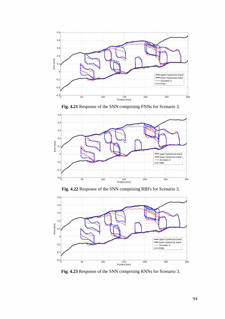
94

0 50 100 150 200 250 300-0.3

-0.2

-0.1

0

0.1

0.2

0.3

0.4

0.5

Position [mm]

Erro

r [m

m]



0 50 100 150 200 250 300-0.3

-0.2

-0.1

0

0.1

0.2

0.3

0.4

0.5

Position [mm]

Erro

r [m

m]



0 50 100 150 200 250 300-0.3

-0.2

-0.1

0

0.1

0.2

0.3

0.4

0.5

Position [mm]

Erro

r [m

m]



95

As expected, the position estimation errors on major- and minor hysteresis loops are

getting bigger in Scenario 3 since the calculated average velocity on major loop (24

mm/s) significantly differs from that of the training scenario. Furthermore, this case

constitutes cascaded minor loops which deteriorate the performance of the NNs due

to the error contributions of ANNsp networks which predict the starting point of the

new trajectory. Finally, the Figs. 4.24, 4.25, and 4.26 present the overall

performances of the NNs for Scenario 4. The major loop performances of the NNs

for this scenario are worst than those for Scenario 1 and Scenario 2 since the

conditions in this case (e.g. the average velocity of 25.5 mm/s) are significantly

different from the ones in the training session.

0 50 100 150 200 250 300-0.3

-0.2

-0.1

0

0.1

0.2

0.3

0.4

0.5

Position [mm]

Erro

r [m

m]

upper hysteresis bandlower hysteresis bandScenario4FNN


0 50 100 150 200 250 300-0.3

-0.2

-0.1

0

0.1

0.2

0.3

0.4

0.5

Position [mm]

Erro

r [m

m]

upper hysteresis bandlower hysteresis bandScenario4RBF


96

0 50 100 150 200 250 300-0.3

-0.2

-0.1

0

0.1

0.2

0.3

0.4

0.5

Position [mm]

Erro

r [m

m]

upper hysteresis bandlower hysteresis bandScenario4RNN


The type of NNs used in the SNN does not have a major influence on the results

owing to the fact that the training errors associated with them are comparable in

magnitude. Consequently, for a TBD that constitutes a large hysteresis band of 300

microns (plus a gearbox backlash of 120 microns), the presented network can

estimate the carriage’s position with an overall root-mean-square error of 25-35

microns utilizing the position measurements at the actuator (driver) side.

Note that the estimation performance of the SNN utilizing the FNN is slightly better

the others. That is, all RMS error values for FNN on major- and minor loops are

less than 30 μm. This network is presumed sufficient for error compensation in

precision applications (Kulkarni and El-Sharkawi, 2001).

It is evident from Table 4.4 that the main error comes from the transient regimes

(minor loops) where the motion could only be transmitted by friction forces.

Unfortunately, modeling the friction characteristics in such regimes is quite

challenging as it involves a large number of variables including the radial- and axial

vibrations of the belt (Abrate, 1992). For that reason, the developed NN models,

which lack the relevant inputs, could not fully capture the complex micro-slip

phenomenon which is quite dominant in this operating regime. Furthermore, other

97

physical variables (such as belt tension, interface temperature, form errors of the

pinion and belt teeth, etc.) could be incorporated to the developed NN models to

increase the performance. However, such attempts would clearly defy the

practicality (and the goal) of the presented method.

4.7 Closure

In this chapter, a TBD, which is not subjected to any external load, was considered.

It has been shown that the transmission error patterns of such (elastic) mechanisms

are repeatable to a certain extent. Hence, this feature motivates the design of an

estimator that makes good use of indirect measurement techniques.

As suggested by the previous studies, various interpolation paradigms could be used

to compute these (quasi-static) error patterns (possibly in real-time). However, huge

numbers of data points are required to represent the corresponding patterns

accurately. Furthermore, complex decisions are still necessary to switch among

various interpolation schemes. A natural choice is to capture the “essence” of error

patterns via NNs.

As briefly shown in this work, a generic RNN topology could not be developed to

establish the desired relationship effectively within a reasonable time frame. On the

other hand, the study has illustrated the performance of the presented SNN via a

number of practical test cases. Using the sketchy guidance of the model at hand, a

number of smaller NNs (with different architectures like FNN, RBF, RNN) were

designed to tackle with these elementary “mapping” problems. Finally, seven NNs

performing glue logic were designed to combine these individual networks. Hence,

a SNN topology was tailored to estimate the transmission error efficiently.

Despite the fact that the mechanical system under study was far from ideal, the

presented network yielded a satisfactory estimation performance provided that no

external forces were acting on the carriage of the mechanism. Even though this (“no

load”) condition seems to be seriously restricting the application of the presented

paradigm; it is crucial to recall that most mechanisms encountered in practice (e.g.

98

printer/plotters, scanners, plasma/laser beam cutters, rapid prototyping machines,

etc.) do not operate under the presence of external loads. Thus, the presented

approach (which conveniently embodies an actuator with a crude position sensor)

can be easily incorporated to the advanced motion controllers for such applications.

99

CHAPTER 5

PRESSURE PREDICTION OF A SERVO-VALVE

CONTROLLED HYDRAULIC SYSTEM 5.1 Introduction

Hydraulic systems are widely used in many applications such as manufacturing

equipment, construction machinery, rolling and paper mills, aircrafts, etc. If

compared to their electrical counterparts, they could provide large forces at higher

speeds with a high power-to-weight ratio. In hydraulic control systems, the relevant

physical quantities such as position, velocity, acceleration, pressure, flow-rate and

actuator force are measured via precision sensors to carry out a specific control task.

Among these quantities, the pressures in cylinder chambers of the electro-hydraulic

servo systems (EHSSs) play a key role in both the implementation of closed-loop

force and/or position control and estimation of disturbances on the hydraulic

actuator. Generally, accurate trajectory tracking control of hydraulic actuators is

realized by the application of advanced control techniques such as adaptive robust

control (Yao et al., 2000; Kaddissi et al., 2011; Mohanty and Yao, 2011), cascade

control (Guo et al., 2008) and sliding-mode control (Guan and Pan, 2008; Pi and

Wang, 2011). Despite the fact that position sensors, accelerometers, and force

sensors are frequently utilized for tracking control of hydraulic systems, the above-

mentioned control applications exclusively require the measurement of hydraulic

(actuator chamber) pressures. Note that the introduction of pressure sensors

increases the cost and complexity of the overall control system while reducing its

reliability due to extra sensors and interface circuitry incorporated to the system.

Likewise, in many industrial applications, the number of dedicated pressure sensors

100

(or any other sensors like PZT or strain-gage based load cells for that matter) is

sought to be minimized for the purpose of reducing both the overall cost and the

sensor-related malfunctions. Hence, an accurate pressure dynamic model, which

could also be used for maintenance and fault-detection purposes, may allow a

pressure sensor to be replaced by a relevant model (a soft-sensor or observer).

Note that accurate models for the dominant dynamics of the system must be also

incorporated to the controller design so as to obtain a high bandwidth response

(Jelali, 2003). A dramatic increase in control system performance can be

accomplished via the use of predictive control schemes that employ stable models

to forecast the behavior of the plant in foreseeable future (Lawrynczuk, 2010). On

the other hand, the dynamic behavior of an EHSS is known to be highly nonlinear

due to the compressibility of the hydraulic fluid, the complex characteristics of the

flow-control device (i.e. servo-valve), the friction- and the leakage in the hydraulic

actuators which in turn create problems in the model development efforts / control

for such systems. Yet, nonlinear control system development for EHSSs remains a

challenging task and is an active area in fluid power research (Karpenko and

Sepehri, 2010).

There is not a single study that could predict accurately the long-term pressure

dynamics of a valve-controlled EHSS in the current literature. For instance, Zhang

(1997) and Watton et al. (1997) reveal the problem of creating reliable ANN models

for hydraulic systems. Furthermore, He and Sepehri (1999) deal with the prediction

problem and they were able to predict (15 step ahead) chamber pressures of an

electro hydraulic test setup using a NARMAX-type network with prediction

accuracy about ±5-10 bar (using a pressure sensor with a measurement accuracy of

1% within the range of 0-138 bar). Hence, the objective of this study is to predict

the long-term pressure dynamics of an EHSS without the use of any extra sensors.

The signals, which are exclusively used for the long-term pressure prediction task,

are the control voltage to the servo valve driver and the measured position of the

hydraulic actuator. No doubt, the pressure sensors would be used in the training

operation and then they would have to be removed in the validation phases. This

101

study considers only the problem of design of an ANN model to predict the

chamber pressure variables in a hydraulic cylinder actuator. The long-term

prediction performances of the proposed network are demonstrated through a

number of simulation studies. Therefore, the objective of this study is not only to

elaborate the performance within the framework of realistic case scenarios but also

to study the adaptation of a network model to a new hydraulic system with different

physical parameters.

The rest of the Chapter 5 is organized as follows: Section 5.2 describes the

simulation based hydraulic system employed in this study. Section 5.3 focuses on

the design of RNN architectures to predict the hydraulic pressures using traditional

techniques and utilizing the sketchy guidance of a priori knowledge at hand.

Section 5.4 shows the practical usage of the devised neural network models for a

hydraulic experimental test set up. Finally, concluding remarks are presented in

Section 5.5.

5.2 Hydraulic System Model

The hydraulic actuation system considered in this study is composed of a fixed-

displacement pump, a pressure relief valve, an accumulator, a critical-centered (or

zero lapped) servo-valve and a double-action cylinder that is coupled to a load

operating in a high-friction environment as shown in Fig. 5.1. For the sake of

keeping the study in focus (and succinct), the mathematical models of the pump, the

pressure relief valve, the accumulator and the pipe lines (along with the interactions

among themselves) are not given below. However, the models of these systems are

given in appendix A in a detailed manner.

Consequently, the models of the key hydraulic circuit elements (i.e. servo-valve and

a double-action cylinder) that would allow the development of reduced-order

pressure estimators are to be discussed here. Referring to Fig. 5.1, the nonlinear

(differential) equations describing the relationships among the servo-valve control

flows (QA and QB) and the actuator position (x) can be written as

102

( )fric ext A B pMx Bx Kx F F P P A+ + + + = − (5.1)

( ) ( ).

A A pA

P Q A xV xβ

= − (5.2a)

( ) ( ).

B B pB

P Q A xV xβ

= − + (5.2b)

where Μ is the mass of the piston/load; Β is the effective viscous damping; K is the

stiffness of the equivalent spring, Αp is the piston annulus area and β refers to the

bulk modulus of the hydraulic fluid. PA and PB denote the hydraulic pressures in

each actuator chamber. Note that the volumes of hydraulic oil on each side of the

piston are expressed by VA(x)= VA0+ Apx and VB(x)=VB0− Apx where VA0 and VB0 are

the initial chamber volumes when the piston is located at the center of the cylinder.

Please note that the internal leakage between the chambers of a hydraulic actuator is

generally characterized as a laminar flow (where the associated Reynolds number is

smaller than 2000) and could be given as

( )leakage L A B LQ C P P C P= − = Δ (5.3)

where CL (leakage coefficient) generally ranges in between 10-12m3/(Pa⋅s) (Kaddissi

et al, 2007) and 10-15m3/(Pa⋅s) (Guan and Pan, 2008) for hydraulic actuators.

Despite the fact that CL depends on many different physical parameters, this

important coefficient can be approximately expressed as

3

LDcC

Lμ∝

(5.4)

where D is the piston diameter; c is the clearance between the piston and the

cylinder; μ is the dynamic viscosity coefficient; L is the length of the piston

(Merritt, 1967). As can be seen from (5.4), the clearance has the biggest impact on

103

the leakage flow. In practice, the internal leakage could be omitted if the seal

between the chambers is considered intact. That is, the clearance between the piston

and cylinder is extremely low. Otherwise, the resulting flow will affect the pressure

dynamics and one must incorporate (5.3) to (5.2). In that case, a cross-coupled

pressure model must be utilized. Note that, in this experimental (and simulation)

study, the leakage in the hydraulic actuator is neglected since a brand-new actuator

(with virtually no wear whatsoever) is employed.

The valve flow rates (which depend on the valve displacement from neutral) are

also nonlinear in nature and could be given as

, 0

, 0v v S A v

Av v A T v

K u P P uQ

K u P P u

⎧ − >⎪= ⎨− <⎪⎩

(5.5a)

, 0

, 0v v B T v

Bv v S B v

K u P P uQ

K u P P u

⎧ − >⎪= ⎨− <⎪⎩

(5.5b)

2 /v dK C w ρ= (5.6)

where PS refers to the hydraulic supply pressure and PT denotes the tank (reservoir)

pressure; Kv is the servo-valve flow gain; w is the orifice area gradient of the servo-

valve. The servo-valve orifice coefficient of discharge is given by Cd while ρ

denotes the density of the hydraulic oil. Here, uv refers to the displacement of the

valve spool.

Moreover, the friction force in (5.1) can be characterized by a dynamic friction

process model like the LuGre model (Mihajlov et al., 2002) as

0 1 2fricF z z vσ σ σ= + + (5.7)

( ) ( ) ( ) ( )( )2/

0

1, sv vc s c

vdz v z g v F F F edt g v σ

−= − = + − (5.8)

104

where v is the velocity of the piston; z is an internal state representing the average

bristle deflection; vs is the Stribeck velocity; Fs is the static friction, Fc is Coloumb

friction; σ0 is the bristle-spring constant; σ1 is the bristle-damping coefficient and σ2

is viscous friction coefficient.

AP

BP

AQ

BQ

SP

TP

cV

M

K B

x

extF

Fig. 5.1 Valve controlled hydraulic system.

A servo-valve is a complicated electro-mechanical device that includes a torque

motor, a flapper-nozzle, and a valve spool. The manufacturers of such devices often

times provide (linearized) models that characterize accurately the dynamics of their

devices within the frequency response band of interest. For the servo-valve

considered in this study, the current drive along with the valve-spool dynamics can

be described in Laplace (s) domain as

( )( )

1

c C C

I sV s L s R

=+

(5.9)

( )( )

2

2 22v h n

n n

u s KI s s s

ωζω ω

=+ +

(5.10)

105

In these equations, LC is the valve-coil (solenoid) inductance; RC is the coil

resistance; Vc is the control voltage; I is the current in the coil; Kh is the first stage

servo valve gain. Moreover, ζ and ωn is the damping ratio and natural frequency of

the servo-valve. Manufacturers’ catalogues provides the relevant parameters of

these linear models.

In the simulation study, a fixed-step integration (0.1 ms) was performed via

MATLAB® Simulink using Dormand-Prince solver. The parameters of the afore-

mentioned models are presented in Table 5.1. Note that the advanced simulation

model is primarily used to provide the data needed for not only designing the

structured NNs but also assessing their (preliminary) prediction performance.

Table 5.1 Some of the key model parameters used in the simulation study.

Par. Value Par. Value Par. Value

M 9 kg VA0 0.00005 m3 Kh 0.0401 m/A

B 2000 N⋅s/m VB0 0.00005 m3 ωn 1256 rad/s

K 10 N⋅m β 1.4×109 Pa ζ 0.7

AP 645×10-6 m2 σ0 12×105 N/m LC 0.59 H

Ps 2×107 Pa σ1 300 Ns/m RC 100 Ω

Kv 3.2×10-5 m5/2/kg1/2 σ2 60 Ns/m Qmax 6×10-5 m3/s

Cd 0.625 Fc 100 N uv_max 0.6×10-3 m

w 1.08 mm Fs 130 N xmax 0.05 m

ρ 890 kg/m3 vs 0.1 m/s Imax 15 mA

5.3 Prediction Models and Parameter Estimation

The problem of creating accurate ANN models for the long-term pressure

prediction in the cylinder chambers of a valve-controlled hydraulic system is to be

solved by using black-box- and gray-box (SNN) modeling approaches in Sections

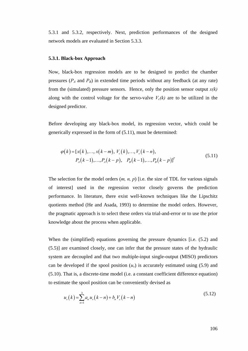
106

5.3.1 and 5.3.2, respectively. Next, prediction performances of the designed

network models are evaluated in Section 5.3.3.

5.3.1. Black-box Approach

Now, black-box regression models are to be designed to predict the chamber

pressures (PA and PB) in extended time periods without any feedback (at any rate)

from the (simulated) pressure sensors. Hence, only the position sensor output x(k)

along with the control voltage for the servo-valve Vc(k) are to be utilized in the

designed predictor.

Before developing any black-box model, its regression vector, which could be

generically expressed in the form of (5.11), must be determined:

( ) ( ) ( ) ( ) ( )( ) ( ) ( ) ( )

[ , , , , , ,

1 , , , 1 , , ]c c

TA A B B

k x k x k m V k V k n

P k P k p P k P k p

ϕ = − −

− − − −

… …

… … (5.11)

The selection for the model orders (m, n, p) [i.e. the size of TDL for various signals

of interest] used in the regression vector closely governs the prediction

performance. In literature, there exist well-known techniques like the Lipschitz

quotients method (He and Asada, 1993) to determine the model orders. However,

the pragmatic approach is to select these orders via trial-and-error or to use the prior

knowledge about the process when applicable.

When the (simplified) equations governing the pressure dynamics [i.e. (5.2) and

(5.5)] are examined closely, one can infer that the pressure states of the hydraulic

system are decoupled and that two multiple-input single-output (MISO) predictors

can be developed if the spool position (uv) is accurately estimated using (5.9) and

(5.10). That is, a discrete-time model (i.e. a constant coefficient difference equation)

to estimate the spool position can be conveniently devised as

( ) ( ) ( )3

1v n v n c

nu k a u k n b V k n

=

= − + −∑ (5.12)

107

where an and bn are the constants of the difference equation.

Note that the selection of sampling period (T) plays a key role in discrete-time

modeling of dynamic systems. Reuter (1995) studies the system identification of

hydraulic servo-systems and shows that a sampling period in between 0.86 ms and

1.3 ms is sufficient for modeling purposes of such systems. Therefore, in this study,

1 ms, which is a common choice in the current state of the art (Yousefi et al., 2008),

is selected as the sampling period. Note that when (5.2) and (5.5) are discretized via

backward difference method (i.e. Euler method), the prediction models simply boil

down to

( ) ( )( ),x x x xP k f kϕ θ= (5.13a)

( ) ( ) ( ) ( )( ) [ , , , 1 ]Tx v xk u k x k v k P kϕ = − (5.13b)

where θx is the weight vector; the subscript x denotes a placeholder for letters A and

B.

Before the training session, one should select a proper excitation signal in order to

create input-output data set. Looking to the literature, it is seen that PRMS is the

most suitable choice of input signal form for identification of hydraulic systems

(Jelali and Kroll, 2003; He and Sepehri, 1999; Xue-miao et al., 2010; Barbosa et al.,

2011). Therefore, the servo-valve manipulation signal, shown in Fig. 5.2.a, is

applied for gathering the training data. Fig. 5.2.b represents the position and

velocity profile of the hydraulic actuator. Furthermore, Figs. 5.2.c and 5.2.d show

the pressure dynamics for this training scenario in chamber A and B, respectively. It

is seen that the pressure dynamics is getting more vibratory when the piston

approaches to its stroke limits (0.05 m) at about 7.8 seconds.

108

0 1 2 3 4 5 6 7 8 9 10-2.5

-2

-1.5

-1

-0.5

0

0.5

1

1.5

2

Time [sec]

Con

trol V

olta

ge [V

]

a) Servo-valve manipulation signal.

0 1 2 3 4 5 6 7 8 9 10-0.02

0

0.02

0.04

0.06

Time [sec]

Posi

tion

[m]

0 1 2 3 4 5 6 7 8 9 10-0.1

-0.05

0

0.05

0.1

Vel

ocity

[m/s

]

positionvelocity

b) Cylinder position and velocity.

0 1 2 3 4 5 6 7 8 9 1095

96

97

98

99

100

101

102

103

104

105

Time [sec]

Pres

sure

[bar

]

c) Pressure dynamics in chamber A.

109

0 1 2 3 4 5 6 7 8 9 10

90

92

94

96

98

100

102

104

106

108

110

Time [sec]

Pres

sure

[bar

]

d) Pressure dynamics in chamber B.

Fig. 5.2 Training data used for the modeling of servo-valve controlled hydraulic

system.

First of all, a NARX model is devised to model the pressure dynamics as can be

seen from Fig. 5.3. The network is trained via MATLAB® (2008a) NN toolbox that

runs on a PC with Intel Core i5 processor and a SDRAM of 4GB. Due to poor

training performance, the regression vector in (5.13.b) is modified as

( ) ( ) ( ) ( ) ( ) ( ) ( ) ( ) ( )[ , 1 , , 1 , , 1 , 1 , 2 ]Tx v v x xk u k u k x k x k v k v k P k P kϕ = − − − − − (5.14)

Table 5.2 summarizes the properties of this network. Even though this model

exhibits excellent training performance, the resulting network alone is of little

practical use owing to the fact that the model requires the history of the pressure

state. It is important to note that a fully recurrent neural network, which produces

self-sustaining predictions, cannot be trained to the desired accuracy when the

weights of the network are initialized randomly. As for the next step, the output of

this network is directly fed back as could be seen from Fig. 5.3. The resulting

network, which is commonly referred to as NOE model, is further trained via RTRL

algorithm. The summary of the training session is also given in Table 5.2. Hence,

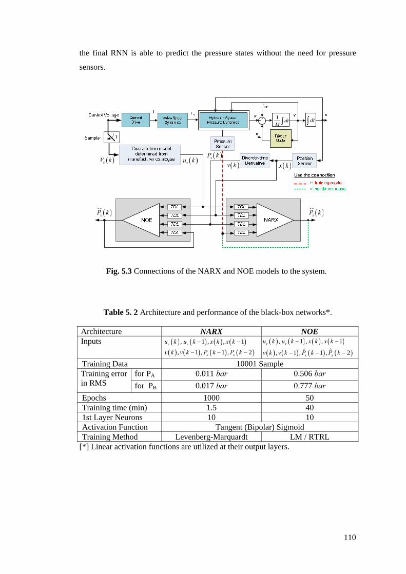
110

the final RNN is able to predict the pressure states without the need for pressure

sensors.

( )xP k( )vu k

( )v k

( )xP k

( )cV k( )x k

dt∫1 dtM ∫

( )xP k

Fig. 5.3 Connections of the NARX and NOE models to the system.

Table 5. 2 Architecture and performance of the black-box networks*.

Architecture NARX NOE Inputs ( ) ( ) ( ) ( )

( ) ( ) ( ) ( ), 1 , , 1

, 1 , 1 , 2v v

x x

u k u k x k x k

v k v k P k P k

− −

− − −

( ) ( ) ( ) ( )( ) ( ) ( ) ( )

, 1 , , 1ˆ ˆ, 1 , 1 , 2

v v

x x

u k u k x k x k

v k v k P k P k

− −

− − −

Training Data 10001 Sample Training error in RMS

for PA 0.011 bar 0.506 bar for PB 0.017 bar 0.777 bar

Epochs 1000 50 Training time (min) 1.5 40 1st Layer Neurons 10 10 Activation Function Tangent (Bipolar) Sigmoid Training Method Levenberg-Marquardt LM / RTRL


111

5.3.2 Gray-box (SNN) Approach

A close examination of the (simplified) model presented in Section 5.2 reveals that

it can be conveniently divided into two parts: flow-rate model and pressure model.

Hence, the pressure states may be predicted accurately when the flow-rates for each

chamber (rather than uv(k) input) is provided. Fig. 5.4 illustrates the schematic of

the proposed structured recurrent neural network where 1 _ max max/v v SG K u P Q=

and ( ) ( )2 max 0x SG Q T V Pβ= refers to two gains with lumped parameters. The

following sections elaborate the NN designs in the topology.

Network Qa

( )vu k

Network Qb

Network Pa

Network Pb

_ max1/ vu

( )v k

SP

( )BP k

( )AP k1G

Laye

r 1a

Laye

r 2a

Laye

r 3a

Laye

r 1b

Laye

r 2b

Laye

r 4a

Laye

r 5a

Laye

r 4b

Laye

r 5b

SP

2G

maxpA Q

( )x k 0p xA V

1G

Laye

r 3b

2G

Δ

Δ

Fig. 5.4 Schematic of the structured recurrent neural network.

5.3.2.1 Flow-rate Model

Flow-rate can be estimated by a NN model using a priori information about the

process. If the pressure states in (5.5) are normalized by the maximum pump supply

pressure (PS) while the spool displacement is scaled by the maximum allowable

valve-spool displacement (uv_max), the nonlinear flow characteristic [as expressed by

(5.5) in its simplified form] can be learned by a FNN. That is, training data set (i.e.

normalized flow rate) could be generated for all the ranges of normalized pressure

112

and spool position. Presuming that the normalized pressure is available, a FNN can

be trained to learn this nonlinear mapping.

Table 5.3 summarizes some of the FNN architectures considered in this study. As

can be seen, the fourth architecture, which yields the minimum root-mean-square

(RMS) training error, is utilized to estimate the corresponding flow rates (see the

networks labeled Network Qa and Network Qb in Fig. 5.4).

It is critical to notice that to estimate the flow rate at time instant kT, the network

requires not only the valve-spool displacement (uv) but also the pressure estimate at

t = kT. Since such an estimate is usually not available for that instant, the previous

value of that state must be employed for all intensive purposes. Hence, this practical

implementation necessity implies that the pressure does not change significantly

within one sampling interval and that Px(k) ≅ Px(k-1).

Table 5.3 Characteristics of various networks designed for QA*.

Architecture # 1 # 2 # 3 # 4 1st layer neurons 10 30 5 10 2nd layer neurons - - 5 10 Output layer neurons 1 1 1 1 Number of epoch 1000 1000 1000 2500 Training time in (min) < 1 < 3 < 1 < 7 RMS training error in (m3/s) 4.37 ×10-7 5.22 ×10-8 2.31 ×10-7 8.52 ×10-9

Training data 9801 Sample Training method Levenberg-Marquardt Activation function Tangent (Bipolar) Sigmoid


5.3.2.2 Pressure Model

Once the flow rates are estimated to the desired accuracy, the chamber pressure

(rates) can be approximately computed via (5.2) in a straightforward fashion.

Considering the discrete-time equivalent of (5.2) [as computed via a Euler

integration method], a RNN should implement the below pressure dynamics as

113

( ) ( )( )

A pA A

A0 p

Q k A v kP (k)=P (k-1)+T

V A x kβ⎡ ⎤−⎢ ⎥

+⎢ ⎥⎣ ⎦ (5.15a)

( ) ( )( )

B pB B

B0 p

Q k A v kP (k)=P (k-1)+T

V A x kβ⎡ ⎤− +⎢ ⎥

−⎢ ⎥⎣ ⎦ (5.15b)

One needs to design a specific FNN to implement the division operation in (5.15)

since it is tested and seen that a generic RNN could not learn the pressure dynamics

directly using a regression vector whose elements constitute from Qx(k), ,x(k), v(k)

and Px(k-1).For that purpose a FNN, called divider network, is trained with

normalized inputs in such a way that Ω is between [-1 +1] and Γ is between [-0.9

+0.9]. This network model will be used as the main part of the pressure model as

shown in Fig. 5.5.

±±( )xQ k

( )v k

( )x k

1Ω± Γ

Ω

Γ

max1 Q

maxpA Q

0p xA V

max

0x

QV

βS

TP +

+SP

( )xP k

Δ

Fig. 5.5 Schematic of the pressure model.

The overall pressure model could be represented with a 2 layered RNN model as

given below

( ) ( ){ } ( )2 2 1 1x xP k G W W k b P kψ ϕ= + + −⎡ ⎤⎣ ⎦ (5.16a)

( ) ( ) ( ) ( ), ,T

xk Q k v k x kϕ ⎡ ⎤= ⎣ ⎦ (5.16b)

114

where Ψ(⋅) is the activation vector function (bipolar sigmoid); the weight matrices

are W1 ∈ ℜ20x3, W2 ∈ ℜ1x20, and bias vector is b ∈ ℜ20x1. As described before, G2 is

a constant in (5.16a) and comes into existence due to the normalization procedure.

Two pressure models, named as Network Pa and Network Pb, are created based on

this architecture and 20 tangent sigmoid neurons are used in the 1st layer of these

network models. After training a number of modular NN models using the “divide-

and-conquer” approach, these subsystems are combined to construct a unified

SRNN. Therefore, a specific network architecture for that system is established. The

SRNN network could be further trained in the unified form for fine tuning of its

weight parameters. It is seen that the training error of the SRNN for PA decreases

from 0.396 bar level to 0.190 bar level within 5 epochs while training session lasts

about 85 minutes. Table 5.4 summarizes the training properties of the SRNN

network. The performance of the resulting network is evaluated in the next section.

Table 5.4 Properties of the structured recurrent neural network.

Input(s) ( ) ( ) ( ),vu k x k v k Output(s) ( ) ( ),A BP k P k

Layer 1a 10 Tangent Sigmoid Layer 2a 10 Tangent Sigmoid Layer 3a 1 Linear Layer 1b 10 Tangent Sigmoid Layer 2b 10 Tangent Sigmoid Layer 3b 1 Linear Layer 4a 20 Tangent Sigmoid Layer 5a 1 Linear Layer 4b 20 Tangent Sigmoid Layer 5b 1 Linear Error of the SRNN after unification

for PA 0.396 bar

for PB 0.773 bar number of training data 10001 Sample

training method LM / RTRLnumber of epoch 5 training time 85 minute Error of the SRNN after training

for PA 0.190 bar for PB 0.598 bar

115

5.3.3 Prediction Results

To assess the prediction performances of the developed RNNs, a validation study

(called v1) is conducted via generating a servo-valve manipulation signal that

constitutes another PRMS as depicted in Fig. 5.6. With this input applied to the

detailed model in Fig. 5.1, the hydraulic system is simulated and a 5000 step-ahead

prediction test is realized with the SRNN and NOE models.

0 0.5 1 1.5 2 2.5 3 3.5 4 4.5 5-4

-3

-2

-1

0

1

2

3

4

Time [sec]

Con

trol V

olta

ge [V

]

Fig 5.6 Servo-valve manipulation signal used in model validation.

Note that in the simulation study, the sensor- and data conversion dynamics are also

taken into consideration. The networks are only provided with the relevant digital

information: x(k) and Vc(k). In this scenario, the position of the piston x(k) is

assumed to be measured by a linear scale with a resolution of 5 microns. Similarly,

the velocity v(k) (as required by the networks) is to be estimated via a first-order

backward difference: ( ) [ ( ) ( 1)]v k x k x k T= − − . Furthermore, the servo-valve

manipulation voltage Vc(k), which is to be generated by a digital control system, is

sampled and converted to the digital representation via a 12-bit analog-to-digital

converter (ADC). Therefore, the inputs to the networks do constitute quantization

noise to some extent.

116

Model validation results are presented in Fig. 5.7 for the NOE and SRNN models.

Fig. 5.7.a represents the temporal pressure changes of chamber A as calculated from

the simulated system’s response (i.e. exact pressure change) for SRNN and NOE

model. Fig. 5.7.b illustrates the accuracy frequency response function (FRF) that is

spectrally averaged to reduce the noise content.

Similarly, Figs. 5.7.c and 5.7.d show the (temporal) pressure changes of chamber B

as well as the corresponding accuracy FRFs. From accuracy FRFs, it has been

observed that the SRNN model outputs are very close to actual states (since the

ratio is about 1). Furthermore, the RMS errors of the SRNN model are 0.552 and

0.43 bars for prediction of PA and PB respectively while the corresponding RMS

errors of the NOE model are 5.592 (for PA) and 2.946 bars (for PB) respectively.

0 0.5 1 1.5 2 2.5 3 3.5 4 4.5 5-20

0

20

40

60

80

100

120

Time [sec]

Pres

sure

[bar

]

exact PASRNNNOE

2.1 2.12 2.14 2.16 2.18 2.2 2.22 2.24 2.26 2.28 2.394

95

96

97

98

99

100

101

102

103

104

105

a) Pressure change in chamber A.

117

10-2 10-1 100 101 102

0.8

1

1.2

Frequency (Hz)

Am

plitu

de

10-2 10-1 100 101 102-20

0

20

40

Frequency (Hz)

Phas

e (d

eg)

NOESRNN

NOESRNN

b) Accuracy frequency response functions when predicting PA.

0 0.5 1 1.5 2 2.5 3 3.5 4 4.5 5-20

0

20

40

60

80

100

120

Time [sec]

Pres

sure

[bar

]

exact PB

SRNNNOE

2.1 2.12 2.14 2.16 2.18 2.2 2.22 2.24 2.26 2.28 2.397

98

99

100

101

102

103

104

c) Pressure change in chamber B.

10-2 10-1 100 101 1020.8

0.9

1

1.1

1.2

Am

plitu

de

10-2 10-1 100 101 102

0

10

20

30

Frequency (Hz)

Phas

e (d

eg)

NOESRNN

NOESRNN

d) Accuracy frequency response functions when predicting PB.

Fig. 5.7 Validation test (v1) results.

118

It is critical to note that all conditions in the validation test v1 (including the

friction) are exactly the same as those of the training case. Consequently, another

verification test (called v2) is carried out for a different set of mechanical system

parameters. That is, the LuGre model parameters in the simulation are changed to

increase the friction force four times if compared to the previous case. Furthermore,

a load (external) force (in the form of a chirp signal with amplitude of 3000 N and a

frequency range from 0.1 Hz to 5 Hz in 5 seconds) is applied to load in order to

fluctuate the chamber pressures in a broader range (70-130 bar) around PS/2 level

(100 bar). The results of this validation scenario are presented in Fig. 5.8. Again,

the pressure changes in both chambers are shown in Figs. 5.8.a and 5.8.b. Not

surprisingly, the SRNN, which apparently captures the essential features of the

hydraulic system, yields excellent long-term prediction performance (where the

RMS error is 0.758 bar and 0.540 bar for the prediction of PA and PB, respectively)

while the NOE model fails to predict the pressure states accurately. It could be

inferred that the estimation accuracy at the frequency band of interest (including

extrapolation capability) of the SRNN models are quite exceptional as indicated by

the accuracy FRFs of the SRNNs in Fig. 5.8.c.

0 0.5 1 1.5 2 2.5 3 3.5 4 4.5 5-150

-100

-50

0

50

100

150

Pres

sure

[bar

]

Time [sec]

exact PA

SRNNNOE

1.3 1.35 1.4 1.45 1.5 1.55 1.685

90

95

100

105

110

115

120

125

130

a) Pressure change in chamber A.

119

0 0.5 1 1.5 2 2.5 3 3.5 4 4.5 5

0

50

100

150

Time [sec]

Pres

sure

[bar

]

exact PB

SRNNNOE1.4 1.45 1.5 1.55 1.6 1.65

70

75

80

85

90

95

100

b) Pressure change in chamber B.

10-2 10-1 100 101 1020.98

0.99

1

1.01

1.02

Frequency (Hz)

Am

plitu

de

10-2 10-1 100 101 102-5

0

5

Frequency (Hz)

Phas

e (d

eg)

SRNN PB

SRNN PA

SRNN PB

SRNN PA

c) Accuracy frequency response functions of the SRNN.

Fig.5.8 Validation test (v2) results.

Moreover, the robustness of the SRNN is tested via applying an external force. Fig.

5.9.a shows the applied external force in time domain while the magnitude of the

(time-varying) prediction errors in chambers A and B are presented in Figs. 5.9.b

and 5.9.c, respectively. A (sampled) cross-correlation coefficient between external

force and prediction error is also calculated as

120

( )( ) ( )( )

( )( ) ( )( )1

2 2

1 1

N

ext extkN N

ext extk k

F k F e k eR=

F k F e k e

=

= =

⎡ ⎤− −⎣ ⎦

− −

∑

∑ ∑ (5.18)

where extF is the mean of applied external force and e is the mean of prediction

error. It is found that the cross-correlation coefficient is 0.076 (7.6%) for prediction

error in chamber A and -0.116 (11.6%) for prediction error in chamber B,

respectively. Furthermore, Fig. 10 shows the prediction error (in bars) of the SRNN

while applying sinusoidal type external forces with different amplitudes and

frequencies. It has been observed that as the magnitude and frequency of the

external force are increased, the prediction performance of the SRNN slightly

deteriorates. However, there exist a significant potential to improve the training

performance of the resulting network via an enhanced training data set (at the

expense of increased training time).

0 0.5 1 1.5 2 2.5 3 3.5 4 4.5 5

-3000

-2000

-1000

0

1000

2000

3000

Time [sec]

Exte

rnal

For

ce [N

]

a) Applied external force.

121

0 0.5 1 1.5 2 2.5 3 3.5 4 4.5 5-6

-4

-2

0

2

4

6

Time [sec]

Pred

ictio

n Er

ror [

bar]

b) Prediction error in chamber A.

0 0.5 1 1.5 2 2.5 3 3.5 4 4.5 5-3

-2

-1

0

1

2

3

Time [sec]

Pred

ictio

n Er

ror [

bar]

c) Prediction error in chamber B.

Fig. 5.9 Test for sampled cross-correlation between external force and prediction error.

Fig. 5.10 Prediction error (in bars) of the SRNN to the applied external force.

122

The above-mentioned claim merely states the fact that if the neural network based

predictor/estimator/observer was “tuned” (or trained) ideally, its estimation error

would approach to zero (within its bandwidth) even if its inputs (uv, x, v) were

highly correlated with the disturbance (or applied external force). Unfortunately,

the theoretical treatment of the above-mentioned aspect using well-known

techniques such as perturbation analysis, interval analysis, describing function

analysis, harmonic analysis etc. is known to be quite challenging for highly

nonlinear systems (i.e. systems with a number of discontinuities). For instance,

devising even an operating-point model for the (simplified) hydraulic system

considered in this study is not straightforward. To be specific, one cannot develop a

linear time-invariant (LTI) (operating point) model when the servo-valve is

operated at its neutral point (uv = 0) while the piston is to be centered around a

specific location (x = x0). Consequently, one needs to employ further assumptions in

order to perform a manageable analysis. To that end, let us assume the followings:

1) Piston is operated at the middle section of the hydraulic cylinder. The

volume changes (in both chambers) as a function of piston position are

presumed negligible.

2) Friction force and linear elastic force component (i.e. spring force) are

embedded to the external force.

3) Piston is assumed to be extending with uv>0.

After defining the perturbation variables as uv = uv0 + δuv (uv>0), v = v0 + δv, PA =

PA0 + δPA, Fext = Fext0 + δFext …; one can “linearize” (5.2) and (5.5) via Taylor

series expansion to get

( ) _

_ _

1 2

3 3

uA ext pA v

A APA ext PA ext

A Av

A A

K AP j u vV Vj K j K

k ku vj k j k

δ ω δ δω ω

β β

δ δω ω

= −+ +

−+ +

(5.19a)

0

_

/ 2

/ 2v vA S

AuA ext v S

u uvP P

QK K Pu =

=

∂=

∂ (5.19b)

123

0

0_

/ 22v v

A S

A v vPA ext

u uA SP P

Q K uKP P=

=

∂=

∂ (5.19c)

where the excitation frequency is ω = 2πf (rad/s) (0 < f < fbandwidth). The terms

KuA_ext and KPA_ext are referred to as the valve spool position gain and the valve

pressure gain of the orifice respectively. In practice, the valve spool position (i.e.

control input voltage) along with actuator velocity is correlated to the external force

provided that a motion-control loop is realized. That is, δuv ∼ δFext and δv ∼ δFext.

Assuming that the neural network based predictor closely mimics the actual

pressure dynamics, the pressure prediction error in chamber A could be defined as

1 1 2 2

3 33 3

ˆ ˆˆ

ˆ ˆA A A A

A A A vA AA A

k k k ke P P u vj k j kj k j k

δ δ δ δ δω ωω ω

⎛ ⎞ ⎛ ⎞− = − − −⎜ ⎟ ⎜ ⎟⎜ ⎟ ⎜ ⎟+ ++ +⎝ ⎠ ⎝ ⎠

(5.20)

Here, the quantities with ^ denote the ones associated with the SNN model. It is

clear from the equation above that δeA → 0 as model coefficients converge to the

actual system parameters ( )1 1 2 2 3 3ˆ ˆ ˆ, ,A A A A A Ak k k k k k→ → → . In that case, the

prediction error would be independent from the external force (i.e. its amplitude and

excitation frequency). As mentioned previously, the SRNN in this study were not

trained perfectly since the training session had to be terminated when the

corresponding error reached a predetermined threshold value. For the sake of

creating a practical training scenario, the data set included only a limited number of

operation regimes where the application of the external force and wideband

excitation of the system via this force was also excluded. As explained before, the

duration of the training session grows exponentially as the network size (i.e. free

parameters) along with the size of the training data set step up dramatically. Under

the given circumstances, one might expect some correlation (or functional

dependence) between the external force and the prediction errors of the developed

network.

124

5.4. Long-term Pressure Prediction of an Experimental Hydraulic Test Setup

The black-box- and gray-box (SNN) modeling approaches devised in Section 5.3

are to be evaluated experimentally and thus this section focuses on the practical

usage of the devised SRNN using an experimental hydraulic test set up.

5.4.1. Experimental Test Setup

The experimental test set up used in this study is illustrated in Fig. 5.11. This set up

was assembled for the evaluation of state feedback control techniques on two

different operating modes (valve controlled and variable-speed pump controlled

mode) of a hydraulic system (Caliskan, 2009). These two circuit schemes can be

selected at will. The components of this setup are listed in Table 5.5.

Fig. 5.11 Experimental test setup (Caliskan, 2009).

Since the presented study concentrates on the pressure estimation of the valve

controlled hydraulic circuit, the experimental set up shown in Fig. 5.12 is operated

in that mode. Note that in this test set up, a double acting asymmetric cylinder is

used as the hydraulic actuator where it is rigidly connected to a steel plate being

Servo-Solenoid Valve

Servo Motors

PumpsPosition Transducer

HydraulicCylinder

Oil Tank

Steel Plate

Pressure Relief Valve

Pressure Transducers

Valve Driver

Motor Driver

125

supported by two sliders at each end to restrict its rotation. The masses of the steel

plate and cylinder rod and the friction acting on the seals of the actuator and the

bearings of the supports constitute the load. The pumps are driven in one direction

with constant speed and their outlet pressure (i.e. the supply pressure of the valve) is

limited by the pressure relief valve. Similarly, a servo solenoid valve regulates the

flow rate through the double acting asymmetric cylinder. The valve driver has a

spool position controller accepting spool position feedback from the LVDT on the

valve and receives its reference spool position command (±10 V). The position of

the actuator, the chamber pressures of the hydraulic cylinder and the valve supply

pressure are measured in the set up. In fact, the spool position of the solenoid valve

can be read from the valve driver via a data acquisition (DAQ) card.

Table 5.5 Components of the hydraulic test setup. Components Remarks Hydraulic pumps Effective displacement: 15.6 cm3/rev

Max. operating pressure: 250 bar Hydraulic actuator Cap side area: 1963.5 mm2

Rod side area: 1001.4 mm2 Stroke: 100 mm Cap side chamber volume: 154387 mm3 Rod side chamber volume: 82455 mm3

Load Steel plate: 11.6 kg Actuator rod: 0.7 kg

Transmission line elements Steel tubes with diameter 12 mm Hydraulic oil Bulk modulus: 1300 MPa

Kinematic viscosity at 20ºC is 100 mm2/s Servo proportional valve & driver BOSCH 4WRPH

Nominal flow rate: 24 l/min Valve gain: 2.138×10-8 m7/2 (kg1/2.V)

Servo motors and motor drivers Nominal power 1 kW DAQ card National Instruments

16 Analog Input 2 Analog Output

Sensors Pressure sensors 0-400 bar, 4-20 mA output LVDT with ±10 V output

126

AP

BP

AQ

BQ

SP

TP

x

Fig. 5.12 Schematic diagram of the experimental test setup.

5.4.2. Adaptation of Black-box Model

To identify the nonlinear black-box models for the given experimental setup, the

measured servo-valve spool position (control signal) shown in Fig. 5.13.a, is

applied to the valve driver for gathering the regression (i.e. training) data. Fig.

5.13.b shows the measured position of the actuator position. As could be seen, the

noise on the position transducer aggravates the noise on the calculated velocity

significantly. Therefore, the position signal must be filtered before the velocity

calculation operation. For this purpose, a discrete-time low-pass filter with a cut-off

frequency of 20 Hz is used to smooth the position signal. Fig. 5.13.c presents the

calculated actuator velocity (which is an element in the regression vector) from the

filtered actuator position signal using first order difference method (FODM).

Furthermore, the pressure changes in each chamber are presented in Fig. 5.13.d. As

127

can be seen, some noise is also observed in the measured pressure as well as valve

spool position signals due to the (pump) motor drivers. Thus, these signals are

filtered with a discrete-time low-pass filter with a cut off frequency of 100 Hz.

Architecture and training performances of the black-box models are presented in

Table 5.6 for this training case.

Table 5.6 Architecture and performance of the black box networks*.

Architecture NARX NOE Input(s)

( ) ( ) ( ) ( )( ) ( ) ( ) ( )

, 1 , , 1

, 1 , 1 , 2v v

x x

u k u k x k x k

v k v k P k P k

− −

− − −

( ) ( ) ( ) ( )( ) ( ) ( ) ( )

, 1 , , 1ˆ ˆ, 1 , 1 , 2

v v

x x

u k u k x k x k

v k v k P k P k

− −

− − −

Output(s) Px(k) Px(k) Training data 50001 Sample Training error (bar)

for PA 0.021 2.243 for PB 0.024 2.891

Epochs 500 10 Training time (min) 6 225 1st layer neurons 10 10 Activation function Tangent (Bipolar) Sigmoid Training method Levenberg-Marquardt LM / RTRL


0 5 10 15 20 25 30 35 40 45 50-1.5

-1

-0.5

0

0.5

1

Time [sec]

Val

ve S

pool

Pos

ition

[Vol

t]

measured valve spool position signalfiltered valve spool position signal

a) Valve spool position.

128

0 5 10 15 20 25 30 35 40 45 50-5

0

5

10

15

Posi

tion

[mm

]

Time [sec]

measured actuator positionfiltered actuator position

b) Actuator position.

0 5 10 15 20 25 30 35 40 45 50-40

-30

-20

-10

0

10

20

30

40

Time [sec]

velo

city

[mm

/s]

c) Calculated actuator velocity from filtered position signal.

0 5 10 15 20 25 30 35 40 45 500

10

20

30

40

50

60

70

80

Time [sec]

Pres

sure

[bar

]

measured PAfiltered PAmeasured PBfiltered PB

PB

PA

d) Cylinder chamber pressures.

Fig. 5.13 Measured and filtered signals that will be used for training.

129

5.4.3 Adaptation of Gray-box (SNN) Model

Due to similarity in the hydraulic system architecture (including zero-lapped servo

valve), the SRNN devised in Section 5.3.2 can be directly adapted for the long term

pressure prediction of the hydraulic cylinder chambers. However, if the servo-valve

in the experimental setup were of a different type (i.e. an overlapped or under

lapped type), the FNNs estimating the flow rates (i.e. Network Qa and Network Qb)

would have to be modified (or redesigned to be exact) to accommodate the unique

nonlinearities associated with these valves. Furthermore, G1 and G2 weights (see

Fig. 5.4) can be calculated provided that the valve gain constant, maximum spool

displacement, pump supply pressure, maximum flow rate of the valve, bulk

modulus of the hydraulic oil, sampling time of the predictor model and initial

chamber volumes are known. All these values, which could be found in Table 5.5,

are used to form the specific SRNN model for this experimental setup.

Again, the filtered signals presented in Fig. 5.13 are used in the training session of

SRNN. The training results are given in Table 5.7. In fact, the SRNN commences

training in close proximity to an acceptable solution in (huge) multi-dimensional

weight space. Hence, the overall network will quickly converge to the best global

solution within a few epochs. The weights of the SRNN layers from 1a to 5a

(shown in Fig. 5.4) are investigated for the purpose of determining the changes in

free weights after the training. Figs. 5.14, 5.15 and 5.16 show the percentage change

of the bias, input and layer weights of the SRNN with respect to the ones before the

training operation. Note that, in these figures, every square indicates the percentage

change of the (bias/input/layer) weight value associated with a unique neuron in the

specified layer shown along the ordinate. It is observed that overall network could

learn the dynamics of the experimental hydraulic system quite easily by making

only a minor weight changes. It is interesting to note that when this SRNN

architecture is initialized with arbitrary weights, the network totally fail to learn the

dynamic behavior of the system. Therefore, the determination of the right

architecture along with the optimal size of the network is not a sufficient condition

to capture the desired functional relationship.

130

Fig. 5.14 Percentage change of the bias weights with respect to the initial model weights.

( )vu k( )x k( )v k

Fig. 5.15 Percentage change of the input weights with respect to the initial model weights.

From 5ato 1a

From 1ato 2a

From 2ato 3a

From 3ato 4a

From 4ato 5a

Fig. 5.16 Percentage change of the layer weights with respect to the initial model weights.

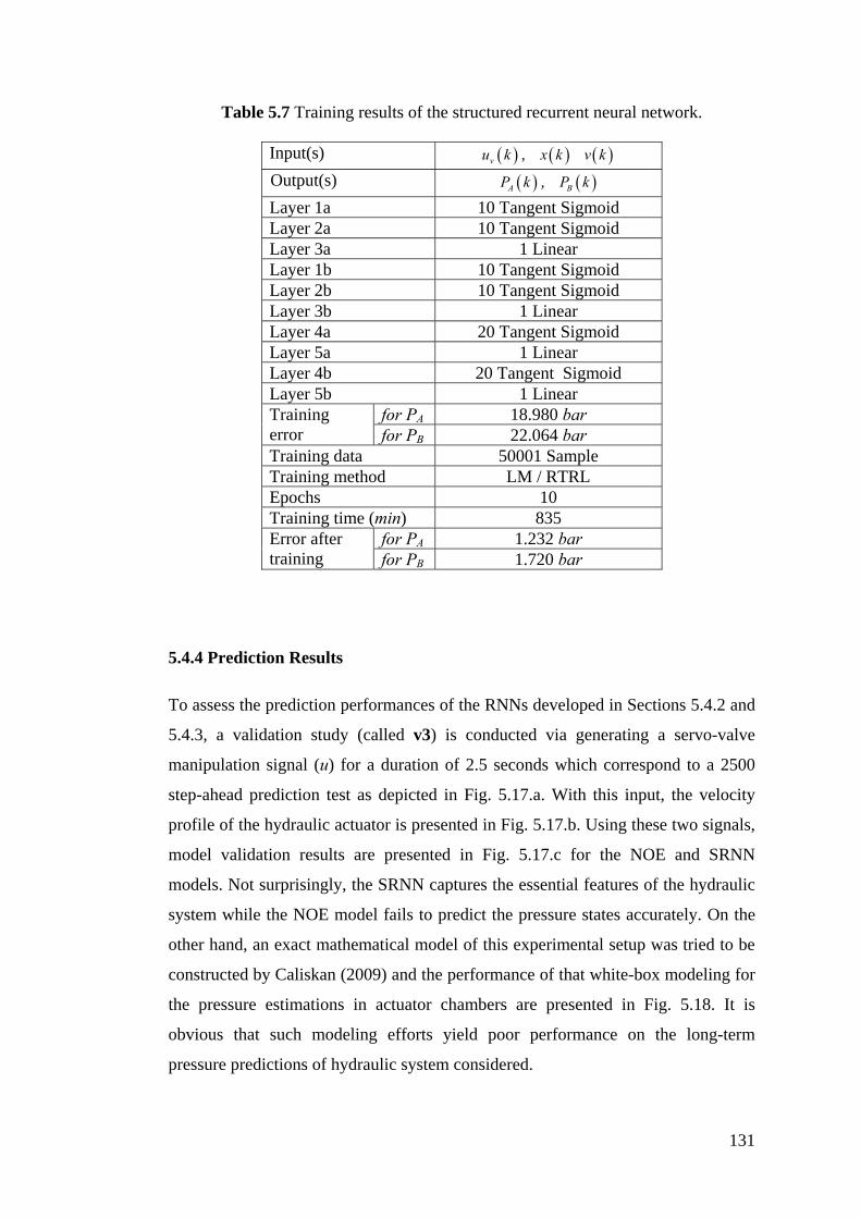
131

Table 5.7 Training results of the structured recurrent neural network.

Input(s) ( ) ( ) ( ),vu k x k v k Output(s) ( ) ( ),A BP k P k

Layer 1a 10 Tangent Sigmoid Layer 2a 10 Tangent Sigmoid Layer 3a 1 Linear Layer 1b 10 Tangent Sigmoid Layer 2b 10 Tangent Sigmoid Layer 3b 1 Linear Layer 4a 20 Tangent Sigmoid Layer 5a 1 Linear Layer 4b 20 Tangent Sigmoid Layer 5b 1 Linear Training error


Training data 50001 Sample Training method LM / RTRLEpochs 10 Training time (min) 835 Error after training



To assess the prediction performances of the RNNs developed in Sections 5.4.2 and

5.4.3, a validation study (called v3) is conducted via generating a servo-valve

manipulation signal (u) for a duration of 2.5 seconds which correspond to a 2500

step-ahead prediction test as depicted in Fig. 5.17.a. With this input, the velocity

profile of the hydraulic actuator is presented in Fig. 5.17.b. Using these two signals,

model validation results are presented in Fig. 5.17.c for the NOE and SRNN

models. Not surprisingly, the SRNN captures the essential features of the hydraulic

system while the NOE model fails to predict the pressure states accurately. On the

other hand, an exact mathematical model of this experimental setup was tried to be

constructed by Caliskan (2009) and the performance of that white-box modeling for

the pressure estimations in actuator chambers are presented in Fig. 5.18. It is

obvious that such modeling efforts yield poor performance on the long-term

pressure predictions of hydraulic system considered.

132

0 0.5 1 1.5 2 2.5-5

-4

-3

-2

-1

0

1

2

3

Time [sec]

Val

ve S

pool

Pos

ition

[Vol

t]

measured valve spool positionfiltered valve spool position


0 0.5 1 1.5 2 2.5-40

-30

-20

-10

0

10

20

30

40

velo

city

[mm

/s]

Time [sec] b) Calculated actuator velocity from filtered position signal.

0 0.5 1 1.5 2 2.50

10

20

30

40

50

60

70

80

Pres

sure

[bar

]

Time [sec]

MeasurementSRNNNOE

PB

PA

c) Cylinder chamber pressures.

Fig. 5.17 Validation study (v3) results.

133

0 0.5 1 1.5 2 2.50

10

20

30

40

50

60

70

80

Pres

sure

[bar

]

Time [sec]

MeasurementWhite-boxmodel

PB

PA

Fig. 5.18 Pressure prediction via white-box modeling approach.

Three more validation tests are realized to check the stability and convergence of

the SRNN model when realizing some closed-loop position control tests on the

hydraulic system. In validation test v4, a 10000 step-ahead prediction test is realized

with the servo-valve signal applied to the servo-valve driver as shown in Fig.

5.19.a. The other necessary signal (the actuator velocity) for the predictor model is

shown in Fig. 5.19.b. Furthermore, Fig. 5.19.c represents the temporal pressure

changes measured by pressure sensors and the predicted ones using the SRNN

model. It is found that the RMS error value of the SRNN model is 1.76 bars for the

prediction of PA and 3.61 bars for the prediction of PB. Moreover, it can be easily

seen that the accuracy FRF of the SRNN model outputs, which are shown in Fig.

5.19.d, are close to actual state for a very broad bandwidth since the ratio is about 1.

134

0 1 2 3 4 5 6 7 8 9 10-6

-5

-4

-3

-2

-1

0

1

2

3

Time [sec]

Val

ve S

pool

Pos

ition

[Vol

t]



0 1 2 3 4 5 6 7 8 9 10-40

-30

-20

-10

0

10

20

30

40

50

velo

city

[mm

/s]

Time [sec] b) Calculated actuator velocity from filtered position signal.

0 1 2 3 4 5 6 7 8 9 100

10

20

30

40

50

60

70

80

90

Pres

sure

[bar

]

Time [sec]

MeasurementSRNN

PA

PB


135

10-2

10-1

100

101

102

103

0.9

0.95

1

1.05

1.1

1.15

Frequency (Hz)A

mpl

itude

10-2

10-1

100

101

102

103

-10

-5

0

5

Frequency (Hz)

Phas

e (d

eg)

SRNN PB

SRNN PA

SRNN PB

SRNN PA

d) Accuracy frequency response functions.


In the next validation test (called v5), the signals that will be used for the validation

of SRNN were shown in Fig. 5.20.a and Fig. 5.20.b, again for a 10000 step ahead

prediction task. The measured and predicted pressures are presented in Fig. 5.20.c

and it is found that the RMS error values of the SRNN are 1.66 bars and 5.48 bars

when predicting PA and PB, respectively. Again, the model accuracy is very high

(prediction error is about 2%) up to frequency of 400 Hz (except at the frequencies

of 35 Hz and 210 Hz) as indicated by the accuracy FRF of the SRNN model

presented in Fig. 5.20.d. It could be said that there is no stability and convergence

problem in the long-term pressure prediction (10000 steps) of the servo-valve

controlled hydraulic system and the validation performance of the SRNN is quite

acceptable.

136

0 1 2 3 4 5 6 7 8 9 10

-4

-2

0

2

4

Time [sec]

Val

ve S

pool

Pos

ition

[Vol

t]



0 1 2 3 4 5 6 7 8 9 10-40

-30

-20

-10

0

10

20

30

40

50

60

velo

city

[mm

/s]

Time [sec]

b) Calculated actuator velocity from filtered position signal.

0 1 2 3 4 5 6 7 8 9 100

10

20

30

40

50

60

70

80

Pres

sure

[bar

]

Time [sec]

MeasurementSRNN

PA

PB


137

10-2

10-1

100

101

102

1030.9

0.95

1

1.05

1.1

1.15

Frequency (Hz)

Am

plitu

de

10-2

10-1

100

101

102

103

-20

-10

0

10

20

Frequency (Hz)

Phas

e (d

eg)

SRNN PB

SRNN PA

SRNN PB

SRNN PA

d) Accuracy frequency response functions.


In the last validation test scenario (called v6), the reference- (command) and the

measured position of the actuator are illustrated in Fig. 5.21.a while the other input

signals (e.g. the valve position and the velocity of the actuator) for the SRNN are

shown in Figs. 5.21.b and 5.21.c. Similarly, Fig. 5.21.d represents the measured

pressure changes and the predicted ones using the SRNN model during a very long-

prediction period (50000 steps). It is found that the SRNN outputs are in good

agreement with the actual pressure states as the corresponding RMS error values

simply become 2.646 bars and 3.496 bars in the cylinder chamber A and B,

respectively. Finally, Fig. 5.21.e illustrates the accuracy FRF of the SRNN for the

frequency band of interest. Consequently, the prediction performance of SRNN for

this experimental case is quite acceptable for all practical purposes. Hence, the

SRNN demonstrates its potential in predicting the chamber pressures for a servo-

valve controlled hydraulic system in extended time periods.

138

0 5 10 15 20 25 30 35 40 45 50-3

-2

-1

0

1

2

3

Time [sec]

Posi

tion

[mm

]

referencemeasurement

a) Reference and measured actuator position signal.

0 5 10 15 20 25 30 35 40 45 50-10

-8

-6

-4

-2

0

2

4

6

Time [sec]

Val

ve S

pool

Pos

ition

[Vol

t]

b) Valve spool position.

0 5 10 15 20 25 30 35 40 45 50-80

-60

-40

-20

0

20

40

60

80

Time [sec]

Vel

ocity

[mm

/s]

c) Calculated actuator velocity from filtered actuator position signal

139

0 5 10 15 20 25 30 35 40 45 500

10

20

30

40

50

60

70

80

90

Pres

sure

[bar

]

Time [sec]

measured PA

measured PB

SRNN PA

SRNN PB

d) Cylinder chamber pressures predicted by SRNN.

10-2 10-1 100 101 1020.9

0.95

1

1.05

1.1

Frequency (Hz)

Am

plitu

de

10-2 10-1 100 101 102-4

-2

0

2

4

Frequency (Hz)

Phas

e (d

eg)

SRNN PB

SRNN PA

SRNN PB

SRNN PA

e) Accuracy frequency response functions.


5.5 Closure

This study presented a NN-based modeling/identification procedure to predict the

long-term pressure dynamics of a valve controlled EHSS. Apart from well-known

black-box approaches (NARX and NOE), the study includes a gray-box approach in

which a SRNN is employed. The developed black-box models consists of a NN

with one hidden layer of sigmoidal neurons and a linear output neuron for the

purpose of mapping the regression vector to the predicted chamber pressures. Even

though the black-box models yielded acceptable training performance, they have

140

failed to predict the chamber pressures in the validation scenarios. Therefore, black-

box model development paradigms to capture the essence of the pressure dynamics

have significant drawbacks.

As an alternative, a gray-box model, which makes good use of a priori information

on the process, is developed. In this approach, a specialized network is devised with

the sketchy guidance of the mathematical models available. Hence, the pressure

dynamics of the EHSS was divided into its sub-systems based on the available

mathematical model. Later, a number of smaller neural networks (i.e. flow-rate

models and pressure models) were designed in order to capture the assigned task on

them. Then, all these networks were combined to yield a tailored SNN (namely

SRNN) for the solution of challenging long-term pressure prediction task problem.

The prediction performances of the SRNN were evaluated through a number of

(simulation & experimental) case studies. These investigations demonstrated that

the SRNN, which has been developed via strong assumptions on the system,

exhibited much better (long-term) prediction performance if compared to its

counterparts employing weak assumptions. The key points (and contributions) of

the study can be summarized as follows:

• Using advanced modeling/filtering/system identification techniques, the long-

term prediction of the chamber pressures of an EHSS is not fully explored in

the current technical literature. Therefore, the devised SRNN is the first

observer system that can be tailored to capture the long-term pressure

dynamics of such nonlinear systems accurately.

• All the advanced controllers in the current state of the art exclusively require

the measurement of hydraulic (actuator chamber) pressures which in turn

increases the overall cost due to pressure sensors and interface circuitry

incorporated to the system. Therefore, this study, which concentrates on the

accurate estimation of these chamber pressures using ANN models (for the

possibility of eliminating costly sensors), complements these research efforts

in the literature.

141

• Study illustrates the adaptation of the SRNN whose free parameters (i.e.

synaptic weights) are adjusted via a detailed simulation study on a generic

valve-controlled EHSS. The same network (with initial weights intact) was

directly applied to model the pressure dynamics of an actual EHSS. After a

brief training session, this network was able to predict the chamber pressures

of this new experimental system quite accurately (error values of the SRNN

are about ±5 bars) in the long run (50000 steps). Training of the presented

network is efficient since the SRNN quickly converges to the global optimum

point (yielding accurate prediction results) as it does not need to start the

training session in any arbitrary point in the huge weight space. Additionally,

the study also investigated the changes in the free parameters as the

adaptation to the new system (elaborated as experimental test setup)

completed. The study shows that no noticeable changes in the hidden layer

weights are observed. Similarly, the output weights change slightly but have a

considerable influence on the prediction performance of the network.

• The experimental studies revealed that the SRNN could predict the chamber

pressures quite accurately (± 5 bars) in relatively long intervals. Apart from

advanced control applications, designed structured neural networks could be

of special importance in some special applications (like military-, and

aerospace systems) where sensor failures could have detrimental effects.

Therefore, the presented network could reliably serve as a sensor backup

system for degraded mode of operation where some of the pressure sensors in

the hydraulic system malfunction.

142

CHAPTER 6

PRESSURE PREDICTION OF A VARIABLE-SPEED

PUMP CONTROLLED HYDRAULIC SYSTEM 6.1 Introduction

In electro-hydraulic servo-systems, the hydraulic power is either controlled by

throttling principle (using servo-valves) or by volumetric control principle (via

adjusting the rotational speed of a constant-displacement pump by a servo motor or

via adjusting the pump displacement by a swash plate).

The former principle offers good dynamic behavior at the expense of substantial

energy losses at the flow control device. On the other hand, the latter principle

yields increased efficiency with a poor dynamic response. When the emphasis is

placed on the high power transmission with low energy losses (i.e. cost-

effectiveness), variable-speed pump-controlled hydraulic systems are generally

preferred in the drive systems of the contemporary machine systems (Helbig, 2002;

Helduser, 2003; Lovrec and Ulaga, 2007; Lovrec et al., 2008).

As similar to the Chapter 5, the objective of this work is to predict the long-term

pressure dynamics of a variable speed pump controlled hydraulic system as the

pressures in cylinder chambers of a hydraulic actuator are needed in various control

tasks. Again, a structured recurrent neural network is proposed as the solution of

long-term pressure prediction problem after seeing that black-box models could not

deal with such a challenging task at hand.

143

The rest of the chapter is organized as follows: After this brief introduction part in

Section 6.1, a variable speed pump controlled hydraulic system and its model is

given in Section 6.2. Following that, some RNN models are trained in order to

predict the cylinder chamber pressures using black-box- and gray-box modeling

approaches in Section 6.3. Next, Section 6.4 illustrates the practical usage of the

structured RNN (as devised in Section 6.3) on the hydraulic experimental test set

up. Finally, concluding remarks are presented in Section 6.5.

6.2 Pump Controlled Hydraulic System

The hydraulic experimental test setup was explained in Section 5.4.1 in a detailed

manner. In addition, hydraulic circuit of the variable-speed pump controlled mode

of the experimental setup and its position controller topology is now illustrated in

Fig. 6.1.

AP

BP

Aq

Bq

x

2tn

1tn

2p Aq 2p Bq

1p Aq

refx+−

++

2n1γ −

sumpΨ

++

λ

2on

1on

1n

Fig. 6.1 Schematic diagram of the experimental test setup (Caliskan, 2009).

144

6.2.1 Mathematical Model

First of all, the model describing the pump controlled mode of the system must be

devised in order to apply the structured neural network (SNN) methodology (Dolen,

2000). All the relevant equations, which are related to the pressure dynamics of the

hydraulic setup, are elaborated here to reveal the interactions among the sub-

systems.

The flow rates of the pumps are adjusted via manipulating the drive speeds of the

servo-motors in order to control the position of the hydraulic actuator. Pumps rotate

in either direction according to the flow needed by the system. As could be seen

from the controller topology, there are two control loops which regulate the piston

pressure and the position, separately. Therefore, the reference inputs of the

independent controllers are the reference position (xref) and the desired value for the

sum of chamber pressures at steady state (psum) as presented below.

_ _sum A steady state B steady statep P P= + (6.1)

The pressure control-loop is used both to pressurize the cylinder chambers to a

predetermined value and to compensate the pump leakages so as to maintain the

stability of the hydraulic cylinder. Similarly, the offset speeds of pump 1 (n1o) and

pump 2 (n2o) are related to each other as

1 2o on nλ= (6.2)

where λ has a negative value. Furthermore, Ψ is another constant used in the

pressure controller in order to determine the ratio between psum and n2o. The steady

state dynamics of the hydraulic system is utilized to find the value of these

constants.

145

Furthermore, the task of the position control loop is to create a manipulated input

signal n2. The cylinder used in the system is a single rod differential cylinder with

an area ratio defined as

A

B

AA

γ = (6.3)

where ΑA and ΑB are the piston annulus areas in the actuator chambers A and B,

respectively. In this controller topology, the hydraulic cylinder is actually moved by

pump 2. On the other hand, pump 1is only used for the compensation of the

asymmetric flow rate due to this differential cylinder. In order to perform this task,

the ratio between the dynamic pump speeds is defined as

( )1 21n nγ= − (6.4)

As shown in Fig. 6.1, when the pumps rotate in the counter clockwise direction, the

flow continuity equations of this hydraulic system could be written from Fig. 6.1 as

follow

( )2 2p A P t i A B ea Aq D n C P P C P= − − − (6.5)

( )2 2p B P t i A B eb Bq D n C P P C P= − − + (6.6)

1 1p A P t i A ea Aq D n C P C P= − − (6.7)

2 1A p A p Aq q q= + (6.8)

2B p Bq q= (6.9)

where the terms PA and PB represent the hydraulic cylinder cap end side and rod end

side chamber pressures, DP is the pump displacement, Ci is the internal leakage, Cea

146

and Ceb are the external leakage coefficients of the pump 1 and pump 2,

respectively. Moreover, n1t and n2t represent the rotational speed of pump 1 and

pump 2 in terms of revolution per second (rps).

Similar to the servo-valve controlled mode of the hydraulic system, the flow

continuity equations for the cylinder chambers are as below

( )A AA A

V x dPq A xdtβ

= + (6.10)

( )B BB B

V x dPq A xdtβ

= − (6.11)

where β is the bulk modulus of the oil. In (6.10) and (6.11), the hydraulic cylinder

chamber volumes are not constant but do change with the hydraulic cylinder

position as VA(x) = AA x + VA0 and VB(x) = −AB x + VB0 where VA0 and VB0 are initial

chamber volumes when the piston is at the midpoint of the hydraulic cylinder.

Defining the load pressure as shown below

L A BP P Pγ= − (6.12)

The force transmitted to the load becomes

L L Bf P A= (6.13)

Next, the Newton’s 2nd law could be applied to the load as

= + + +L fricf mx bx mg f (6.14)

147

In Eq. (6.14), friction force is defined by again a LuGre model as it is given in (5.7)

and (5.8). The numerical values of the physical parameters used in the simulation

study are presented in Table 6.1.

Table 6.1 Model parameters used in the simulation study.

Parameter Value Parameter Value m 12.3 kg σ0 12x102 N/mm AA 1.9635 mm2 σ1 2.6 Ns/mm AB 1.0014 mm2 σ2 2.6 Ns/mm VAo 1.4258 x105 mm3 Fc 330 N VBo 7.6821 x104 mm3 Fs 360 N Dp 15.6 x103 mm3/rev vs 100 mm/s Ci 1027 mm3/(s⋅MPa) λ -1.2294 Cea 120 mm3/(s⋅MPa) Ψ -0.0265 Ceb 120 mm3/(s⋅MPa) β 1300 MPa

6.3 Prediction Models and Parameter Estimation

In this section, the problem of creating accurate ANN models for the long-term

pressure prediction in the cylinder chambers for a (variable-speed) pump-controlled

hydraulic system is to be handled by black-box- and gray-box (i.e SNN) modeling

approaches. These predictive models are initially developed via simulation data

rather than experimental data due to two main reasons:

First of all, black-box- and gray-box models devised in Sections 6.3.1 and 6.3.2 via

a simulated hydraulic system, whose physical system parameters are close to those

of the actual system, will yield reliable initial conditions (i.e. start-off weights) for

further training of the network via experimental data. Note that, despite the devised

SNN is shown to have optimal architecture (i.e. reduced-order nonlinear state

observer), the resultant network totally fails to yield expectable performance in the

training session if its weights are initialized randomly. That is, the training

148

operation with arbitrary initial weights will increase the possibility of catching by a

local minimum in the huge weight (search) space.

Secondly, the design (and also the training) of the gray-box (namely, SNN)

modeling approach will need (normally) the unmeasured states such as the flow

rates (qA and qB) when the long-term pressure prediction problem is divided into its

fundamental components as will be shown in Section 6.3.2. It is seen that capturing

the exact pressure dynamics of the simulated hydraulic system without the

measurements of the control flow rates is extremely difficult. Since there are no

flow meters on the experimental set-up, the gray-box model is developed first for a

simulation based study and then applied (e.g. trained / fine-tuned and tested) on the

experimental setup.

6.3.1 Black-box Approach

First, some neural networks, using the black-box modeling approach, are to be

devised for the long-term pressure prediction of the cylinder chambers in the

simulated system. It is important to note that only the position of the hydraulic

actuator (x(k)) and the rotational speed of the pumps (n1t and n2t) are used as inputs

to the devised models.

A PRMS type signal, given in Fig. 6.2.a, is applied to system and then, the n1t and

n2t signals are formed based on this n2 signal as shown in Fig. 6.1. Note that psum is

set to 12 MPa in the simulated study. Furthermore, Fig. 6.2.b represents the position

and velocity profile of the hydraulic actuator and Fig. 6.2.c shows chamber

pressures for this training scenario.

149

0 1 2 3 4 5 6 7 8 9 10-10

-8

-6

-4

-2

0

2

4

6

8

10

Time [sec]

Con

trolle

r Out

put

a) Controller signal.

0 1 2 3 4 5 6 7 8 9 10-50

-25

0

25

50

Time [sec]

Posi

tion

[mm

]

0 1 2 3 4 5 6 7 8 9 10-300

-150

0

150

300

Vel

ocity

[mm

/s]

velocityposition

b) Cylinder position and velocity.

0 1 2 3 4 5 6 7 8 9 100

1

2

3

4

5

6

7

8

9

10

Time [sec]

Pres

sure

[MPa

]

PB

PA

c) Pressures in the cylinder chambers.

Fig. 6.2 Training scenario for the variable speed pump controlled hydraulic system.

150

Next, the elements of the input vector of the black-box models should be

determined as in the form given below.

( ) ( ) ( ) ( ) ( ) ( ) ( )( ) ( ) ( ) ( ) ( ) ( )1 1 2 2[ , , , , , , , , ,

, , , 1 , , , 1 , , ]t t t t

TA A B B

k n k n k l n k n k l x k x k m

v k v k n P k P k p P k P k p

ϕ = − − −

− − − − −

… … …

… … … (6.15)

For that purpose, various NARX models, which utilize different order of TDL input

signals, are trained in a feed-forward fashion. That is, the old pressure values

coming from the “simulated” pressure sensors are directly fed to the network as

could be seen from (6.15).

The training performance of these black-box models are summarized in Table 6.2.

Architecture #8 is chosen as the topology for the black-box model since it has the

minimum RMS error value. Note that the training performances all of the NARX

models are very satisfactory since they are utilizing measured pressure states

directly in the regression vector. However, the models must be arranged in recurrent

(feedback) form meaning that the previous pressure values must come from the

network’s output itself in the validation case of which is expected to differ

significantly from the training scenario.

Following that, the outputs of the architecture #8 are delayed as necessary and

connected to its 1st layer. As the architecture of the network is now changed due this

feedback, the resulting network will be named as NOE from that point on. The NOE

could train itself without any problem in a recurrent form provided that the initial

weight values are taken from the NARX model. After a training process (10 epoch)

in which the training duration is 70 minute, it is found that the training error of the

NOE was about 0.2 MPa. Hence, the final NOE network is able to predict the

pressure states without utilizing any pressure sensors. The model validation

performance of the resulting network will be evaluated in Section 6.3.3.

151

Table 6.2 Trained NARX models in black-box approach *.

Architecture #1 #2 #3 #4 #5 #6 #7 #8 #9 Inputs n1t(k)

n2t(k) x(k) v(k)

PA(k-1) PB(k-1)

n1t(k), n1t(k-1) n2t(k), n2t(k-1)

x(k), x(k-1) v(k), v(k-1)

PA(k-1), PA(k-2) PB(k-1), PB(k-2)

n1t(k), n1t(k-1), n1t(k-2) n2t(k), n2t(k-1), n2t(k-2)

x(k), x(k-1), x(k-2) v(k), v(k-1), v(k-2)

PA(k-1), PA(k-2), PA(k-3)PB(k-1), PB(k-2), PB(k-3)

Outputs PA(k) and PB(k) Training error in (MPa) 0.09 0.07 0.07 0.02 0.01 8x10-3 0.01 5x10-3 6x10-3

Training data 10001 Sample for each variable Epochs 1000 2000 Training time (min) 1.5 3 5 2 5 9 6 15 25

1st layer neurons 5 10 15 5 10 15 5 10 15

Act. function Tangent sigmoid Training method Levenberg-Marquardt

* Linear activation function is utilized at the output layers.

6.3.2 Gray-box (SNN) Approach

If the mathematical model of this hydraulic system is examined from Section 6.2.1,

it is seen that the model could be easily separated into two parts: flow-rate model

and pressure model. Fig. 6.3 illustrates the topology of the devised structured

recurrent neural network where ( ) ( )max 0 maxxG q T V Pβ= is a connection gain due

to the normalization operation and the subscript x denotes a placeholder for letters A

and B. Moreover, T denotes the sampling period, again. The modules of the devised

SRNN are explained in the following sections.

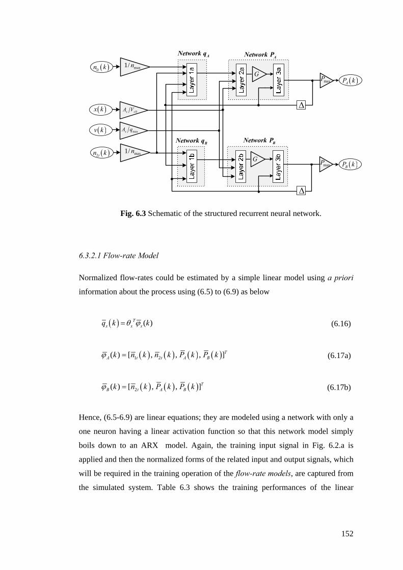
152

( )1tn k max1/ n

( )v k

maxP

( )BP k

( )AP k

maxP

G

maxxA q

( )x k 0x xA V

G

ANetwork qANetwork P

BNetwork PBNetwork q

( )2tn k max1/ n

Δ

Δ

Fig. 6.3 Schematic of the structured recurrent neural network.

6.3.2.1 Flow-rate Model

Normalized flow-rates could be estimated by a simple linear model using a priori

information about the process using (6.5) to (6.9) as below

( ) ( )Tx x xq k kθ ϕ= (6.16)

( ) ( ) ( ) ( )1 2( ) [ , , , ]TA t t A Bk n k n k P k P kϕ = (6.17a)

( ) ( ) ( )2( ) [ , , ]TB t A Bk n k P k P kϕ = (6.17b)

Hence, (6.5-6.9) are linear equations; they are modeled using a network with only a

one neuron having a linear activation function so that this network model simply

boils down to an ARX model. Again, the training input signal in Fig. 6.2.a is

applied and then the normalized forms of the related input and output signals, which

will be required in the training operation of the flow-rate models, are captured from

the simulated system. Table 6.3 shows the training performances of the linear

153

models (labeled as Network qA and Network qB) that are used to predict the flow

rates in each chamber. It is critical to notice that this flow-rate model requires the

pressure estimates at time instant kT. But, such an estimate will not be available at

the desired time while the SRNN is running for a prediction task. Therefore,

pressure estimates at t = (k-1)T will be utilized as the inputs of the flow rate models

assuming that the pressure values are almost same within one sampling interval.

Table 6.3 Trained flow rate models in gray-box approach.

Architecture Network qA Network qB Inputs

( ) ( ) ( ) ( )1 2, , ,t t A Bn k n k P k P k ( ) ( ) ( )2 , ,t A Bn k P k P k

Output ( )Aq k ( )Bq k Training data 10001 Sample Training error in (mm3/s) 2.151x10-6 1.4034x10-6

Epochs 1 1st layer neurons 1 Activation function Linear Training method Least mean square

6.3.2.2 Pressure Model

It is obvious that the chamber pressures could be computed via (6.10) and (6.11) in

a similar way as done in Section 5.3.2.2. Therefore, the same pressure models,

named as Network PA and Network PB, are utilized to solve the pressure dynamics in

the cylinder chambers. It is critical to note that the pressure states are directly taken

from the simulated system and utilized in the regression vector of these models

during the training session in order to increase their training performance. But, all

the related models are then reconfigured in a recurrent arrangement as presented in

Fig. 6.3.

Next, all the modules are connected to each other to form the unified network,

called SRNN. Furthermore, this SRNN model could be trained in the unified form

154

for fine tuning of its weight parameters based on the training scenario. It is seen that

the training RMS error of the SRNN decreases from 0.4 MPa level to 0.2 MPa level

within 5 epochs while training session lasts about 35 minutes. The model validation

performance of the SRNN network is evaluated in the next section.


A validation study is conducted on the simulated system via the rotational speed of

the pumps, realistic input signals which are collected from the experimental setup as

shown in Fig. 6.4.a, are used in the simulated system to create a 50000 step-ahead

prediction task. The hydraulic system presented in Fig. 6.1 is simulated with these

chirp signals (0.1 Hz to 10 Hz in 50 seconds) with increasing amplitude. Fig. 6.4.b

represents the validation performance of the NOE network and it is seen that the

validation performance of this network model is unacceptable for all practical

purposes. On the other hand, Fig. 6.4.c represents the pressure values in the cylinder

chambers calculated from the simulated system model and the SRNN model. It is

found that the RMS errors of the SRNN model are 0.0547 MPa and 0.0911 MPa

for the prediction of PA and PB respectively. Therefore, it could be inferred that the

pressure dynamics of the simulated system is accurately captured by the SRNN

model.

0 0.5 1 1.5 2 2.5 3 3.5 4 4.5 5x 104

-10

-8

-6

-4

-2

0

2

4

6

8

10

Time index k (sample time T=0.001 second)

Rot

atio

nal s

peed

[rps

]

Pump1Pump2

Pump1

Pump2

a) Rotational speed of pumps.

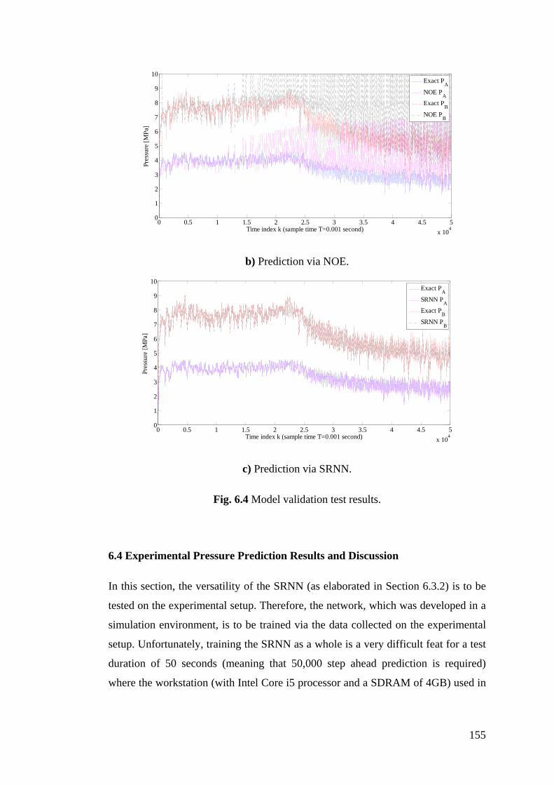
155

0 0.5 1 1.5 2 2.5 3 3.5 4 4.5 5x 104

0

1

2

3

4

5

6

7

8

9

10


Pres

sure

[MPa

]

Exact PANOE PAExact PBNOE PB

b) Prediction via NOE.

0 0.5 1 1.5 2 2.5 3 3.5 4 4.5 5x 104

0

1

2

3

4

5

6

7

8

9

10


Pres

sure

[MPa

]

Exact PASRNN PAExact PBSRNN PB

c) Prediction via SRNN.

Fig. 6.4 Model validation test results.

6.4 Experimental Pressure Prediction Results and Discussion

In this section, the versatility of the SRNN (as elaborated in Section 6.3.2) is to be

tested on the experimental setup. Therefore, the network, which was developed in a

simulation environment, is to be trained via the data collected on the experimental

setup. Unfortunately, training the SRNN as a whole is a very difficult feat for a test

duration of 50 seconds (meaning that 50,000 step ahead prediction is required)

where the workstation (with Intel Core i5 processor and a SDRAM of 4GB) used in

156

the study will be stretched to its limits. For that reason, the SRNN shown in Fig. 6.3

is divided into two (titled as RNN PA and RNN PB) parts and are trained (separately)

to predict the pressure change in each chamber assuming that the opposite chamber

pressure is known in the training session. Figs. 6.5 and 6.6 illustrate the networks in

such a configuration.

( )1tn k max1/ n

( )v k

maxP ( )AP kLa

yer 1

a

Laye

r 2a

Laye

r 3a

G

maxAA q

( )x k 0A AA V

ANetwork qANetwork P

( )1BP k − max1/ P

( )2tn k max1/ n

Δ

Fig. 6.5 RNN PA for the pressure prediction in chamber A.

( )v k

maxP ( )BP k

Laye

r 1b

Laye

r 2b

Laye

r 3b

G

maxBA q

( )x k 0B BA V

BNetwork qBNetwork P

( )1AP k − max1/ P

( )2tn k max1/ n

Δ

Fig. 6.6 RNN PB for the pressure prediction in chamber B.

Next, the formed RNNs are trained using the measured signals that are presented in

Fig. 6.7. That is, the rotational speeds of the pumps are given in Fig. 6.7.a. On the

other hand, Fig. 6.7.b shows the measured position of the cylinder in this training

157

scenario. As could be seen, the noise on the position transducer will aggravate the

noise on the calculated velocity significantly unless any filtering operation is

applied on position signal. Therefore, the position signal is filtered before the

velocity calculation. For that purpose, a discrete-time low-pass filter with a cut off

frequency of 30 Hz is used. Fig. 6.7.c presents the calculated cylinder velocity (as

required in the regression vector) from the filtered actuator position signal using the

first-order difference method. Similarly, the target pressure values and the RNN

outputs after the training operation is given in Fig. 6.7.d while Table 6.4 represents

the training performances of the RNNs. To assess the generalization performance, a

validation scenario, which is illustrated in Fig. 6.8, is considered. As can be seen,

the performances of the RNNs are very satisfactory (since RMS prediction error in

PA is 0.112 MPa and in PB is 0.195 MPa) when the assumption on opposite chamber

pressure is satisfied.

0 0.5 1 1.5 2 2.5 3 3.5 4 4.5 5x 104

-10

-8

-6

-4

-2

0

2

4

6

8

10


Rot

atio

nal s

peed

[rps

]

Pump1Pump2

Pump1

Pump2

a) Rotational speed of the pumps.

158

0 0.5 1 1.5 2 2.5 3 3.5 4 4.5 5x 104

-5

-4

-3

-2

-1

0

1

2

3

4

5


Posi

tion

[mm

]

b) Measured cylinder position.

0 0.5 1 1.5 2 2.5 3 3.5 4 4.5 5x 104

-150

-100

-50

0

50

100

150

Vel

ocity

[mm

/s]

Time index k (sample time T=0.001 second) c) Calculated cylinder velocity from the filtered position signal.

0 0.5 1 1.5 2 2.5 3 3.5 4 4.5 5x 104

-1

0

1

2

3

4

5

6

7

8

9

Pres

sure

[MPa

]


Exact PA

Exact PB

RNN PA

RNN PB

d) Target pressures and model outputs after the training session.

Fig. 6.7 Training signals for the experimental study.

159

Table 6.4 Training properties of the RNNs.

Architecture RNN PA RNN PB Inputs ( ) ( ) ( ) ( ) ( )1 2, , 1 , ,t t Bn k n k P k v k x k− ( ) ( ) ( ) ( )2 , 1 , ,t An k P k v k x k− Output ( )AP k ( )BP k Training data 50001 Sample

Training error 0.092 MPa 0.116 MPa Epochs 10 Training time 365 minute 1st layer neurons 1Linear 2nd layer neurons 20 Tangent Sigmoid 3rd layer neurons 1Linear

Finally, the RNN PA and RNN PB are coupled to each other to form the SRNN.

Therefore, the inputs to the designed model without any feedback (at any rate) from

the pressure sensors will only be the rotational speed of pump 1 and pump 2, the

position and the velocity of the hydraulic cylinder. However, the SRNN outputs

deviate significantly from the chamber pressures measured on the experimental

setup at long intervals as could be seen from the validation performance of this

network given in Fig. 6.9. Since the two outputs of the SRNN are highly cross

coupled to each other, the presented model could not satisfactorily predict the

pressure states in the cylinder chambers. At least, one of the chamber pressure

should be known beforehand to predict the opposite chamber pressure accurately. In

any way, the presented model could be used to predict the pressure in one chamber

quite accurately with an RMS error of 0.2 MPa (where the pressure varies in

between 0 and 10 MPa) when the pressure value of the opposite chamber is

available. Therefore, one of the advantages of the developed SRNN for the

hydraulic system at hand is to reduce the total number of pressure sensors in such

hydraulic systems from two to one or the model could be used as a (software)

sensor backup system when a fault is occurred in one of the pressure sensors.

160

0 0.5 1 1.5 2 2.5 3 3.5 4 4.5 5x 104

-6

-4

-2

0

2

4

6

8


Rot

atio

nal s

peed

[rps

]

Pump1Pump2

Pump2

Pump1

a) Rotational speed of pumps.

0 0.5 1 1.5 2 2.5 3 3.5 4 4.5 5x 104

-20

-15

-10

-5

0

5

10

15

20

Time index k (sampling time T=0.001 second)

Posi

tion

[mm

]

b) Cylinder position.

0 0.5 1 1.5 2 2.5 3 3.5 4 4.5 5x 104

-80

-60

-40

-20

0

20

40

60

80

100

120


Vel

ocity

[mm

/s]

c) Cylinder velocity.

161

0 0.5 1 1.5 2 2.5 3 3.5 4 4.5 5x 104

0

1

2

3

4

5

6

7

8

9

10


Pres

sure

[MPa

]

Exact PAExact PBRNN PARNN PB

d) Measured pressures and RNNs outputs.

Fig. 6.8 Validation test of the RNNs.

0 0.5 1 1.5 2 2.5 3 3.5 4 4.5 5x 104

0

1

2

3

4

5

6

7

8

9


Pres

sure

[MPa

]

Exact PASRNN PAExact PBSRNN PB

Fig. 6.9 Validation test of the SRNN.

Another interesting point worth mentioning is that when this SRNN architecture is

to be trained by starting off with an arbitrary set of initial weights, the network

could not capture the dynamic behavior of the system. Therefore, determining the

optimal architecture (size, correct regression vector, etc.) does not guarantee the

solution of the estimation problem at hand. In fact, the SRNN network, which was

trained initially via the data on simulated plant, can be easily adapted to any

162

experimental case since the resulting network will not start training in any arbitrary

location in the huge weight domain but nearly about the global optimum point.

6.5 Closure

This study presented an SRNN based modeling/identification procedure for the

pressure dynamics of a variable-speed pump controlled electro-hydraulic system.

The signals, used for the long-term pressure prediction task, were the rotational

speed of the pumps, the position and the average velocity of the hydraulic actuator.

A gray-box approach (SRNN) beside the well known black-box approaches (NARX

and NOE) were utilized in the identification process. The study elaborated the

performance of these models through a detailed simulation and experimental cases

where black-box modeling approaches failed to yield acceptable performance even

in the simulation studies. On the other hand, it was seen that the SRNN has showed

excellent performance in the simulation study and has been able predicted the

pressures in both chambers of the cylinder quite accurately in relatively long

intervals (i.e. 50s). Unfortunately, the experimental studies revealed that the outputs

of the SRNN diverged in the extended time periods due to the fact the outputs of the

predictor model were highly coupled to each other and the errors introduced by a

number of sources (e.g. noise in the position sensor, the time delay in the velocity

computation, etc.). However, if a pressure sensor were utilized to provide a

feedback to the network, it was able to estimate the other pressure component quite

accurately without any divergence. Hence, the presented network model could

reliably serve as a sensor backup in certain applications where sensor failures could

have catastrophic consequences.

163

CHAPTER 7

POSITION ERROR PREDICTION FOR CABLE-DRUM

SYSTEMS 7.1 Introduction

Cable-drum mechanisms, which are considered to be a subclass of

friction/traction/capstan drive systems, are commonly used to convert the rotary

motion of a drum into a translational one with the utilization of the friction force

induced at the interface of contacting material pair. Apart from their use in

conventional machines such as printing presses, textile machinery, cranes etc;

cable-drum systems are also employed as motion transmission elements in many

precision engineering devices including photocopiers, printers, plotters, rapid

prototyping machines, haptic devices and more. Despite their primary role as power

transmission elements; the cable-drum systems could serve as integral components

of linear position sensors as well. In fact, the mechanisms accommodating an

angular position sensor on the drum shaft do find their commercial uses as

inexpensive sensors for certain industrial applications that do not require high

positioning accuracy such as presses, punching / injection machines, wood- and

sheet-metal working machinery etc. In commercial sensors such as “wire draw

encoders” and “cable encoders”, the cable is often times attached onto a spring-

loaded capstan to create a kinematically-coupled motion. However, the resulting

mechanical system becomes quite complicated (Kautz, 1993; Steinich, 2007) to be

suitable for precision products. Judging by the earlier applications; a cable directly

wound on the capstan does have certain advantages over the “wire drawn” devices

164

including its simplicity, ease-of-manufacture, (almost) unlimited travel spans

(range), linearity, wider bandwidth (better frequency response), etc.

Emphasizing power transmission efficiency, dynamic stiffness, and vibrations;

numerous investigations in the literature have directly focused on the capstan drives

that possess some of the characteristics of the cable-drum mechanisms. In fact,

many studies concentrate on the attributes of traction drives as power transmission

elements rather than their measurement characteristics. The earliest known work is

attributed to Euler (1762) who investigated the balance of a string wrapped around a

fixed drum while Grashoff (1883) revised the friction on belt-pulley mechanisms at

steady-state and laid the ground work on the creep theory. In this classical (and

widely adopted) approach, the pulley/drum is divided into two regions. In the first

region (called slip zone), the cable/belt is to creep against the drum which in turn

enables the power transmission via the friction forces produced at the interface in

accordance with the Coulomb friction law. In the second region (commonly referred

to as adhesion zone), the cable/belt is assumed to adhere to the drum and thus no

friction force is developed to transmit the mechanical power between two media.

Fawcett (1981), Johnson (1985) and Gerbert (1999) review and elaborate the

classical creep theory. In fact, the evolution of the theory has continued in time. For

instance, Bechtel et al. (2000) considered the unaccounted inertial effects in the slip

zone. Moreover, Leamy and Wasfy (2002) conducted a detailed analysis on the

belt-drives using a modified Coulomb friction law. On the other hand, shear model

is the second theory, which was first proposed by Firbank (1970). Next, Gerbert

(1996) studied the shear model by considering the extension of the belt. Later, Kong

and Parker (2005) were the first who compared the two theories applied on a two-

pulley system and they proposed an iterative method for calculating the steady state

behavior of the mechanism. Furthermore, Kong and Parker (2006) have

incorporated the compliances of various (like pulley grooves) on belt-drive

dynamics. Lastly, Tu and Fort (2004) considered the effects of lubricants on the

friction between fiber and capstan while Smith (1998) investigated micro-

tribological interactions among various interfaces in a belt-driven data-tape.

165

Comprehensive review of the relevant literature reveals that the evaluation of the

cable-drum mechanism within the context of precision motion/sensing are not fully

stuied. Only, Werkmeister and Slocum (2007) looked into the (dynamic) stiffness of

a wire capstan drive through a rigorous analytical and experimental study. Based on

this study, Baser and Konukseven (2010) developed an analytical method in order

to calculate the slippage between the cable and drum. It was seen that the analytical

method, whose parameters were determined in an accurate way, could only predict

the slippage within 10% difference from the experimental results. As a result, the

resulting analytical method could not be used for position error estimation for cable-

drum systems since some parameters (such as eccentricity of the drum and friction

coefficient between the cable and drum) and variables ( such as external load and

preload on the cable) must be measured in order to manipulate the calculations.

Furthermore, external load on the cable and also the reference velocity profile of the

output drum were constant in the above-mentioned study; therefore, it eliminates all

the inertia effects and velocity dependent slip dynamics of the device. However,

Kilic et al. (2011) show that the slippage between the cable and drum is highly

dependent on the velocity of the output drum and the external load on the cable

which are continuously changing during the operating conditions of the mechanism.

Therefore, it is seen that the applicability of the analytical method to predict the

transmission error due to slippage is not feasible. Eventually, the main objective of

this study is to devise a practical position error prediction scheme for cable-drum

mechanisms that accept only a position signal from a rotary encoder coupled to the

drum itself.

After this detailed introduction, Section 7.2 introduces a cable drum mechanism as a

linear motion sensor. Following that, the Section 7.3 introduces a test set-up and

investigates the actual dynamic behavior of the device through an experimental

study. In Section 7.4, ANNs are designed to predict the slippage between the cable

and drum. It is shown that black-box modeling approaches are not sufficient for the

estimation of the slip error of the device and hence a structured recurrent neural

network model is devised and (proposed also) to predict the slippage. Finally, the

166

merit of the proposed network is assessed based on a random input test scenario and

thus the crucial points of the study are discussed in Section 7.5.

7.2 Cable-drum Mechanism as Motion Sensor

A generic mechanism serving as a part of a linear motion sensor is illustrated in Fig.

7.1. In this arrangement, a digital rotary position sensor is directly coupled to the

drum (pulley / capstan). The engagement angle of this drum, which plays a critical

role in the induction of traction force between the cable and the drum, is controlled

by the adjustment wheels shown in the figure. Similarly, the preload adjustment

mechanism, which is usually composed of a helical spring and a screw, can be

utilized to set the cable tension to the desired level. Note that the cable is subjected

to an alternating load as the direction of the mechanism changes. Considering that

the cable does not carry any compressive loads, the preload on the cable must be

selected higher than the magnitude of the alternating load itself.

It is critical to note that the mechanism in Fig. 7.1 can be regarded as a simple belt-

drive where the “creep” of the cable against the drum intrinsically induces the

traction (torque) that creates the rotation of the drum. However, unlike conventional

belt drives, the system under investigation has major differences:

• The center of the drum moves along an axis while the cable velocities at entry

and exit points on the drum are essentially zero.

• Effective friction torque acting on the drum’s shaft due to the sensor + bearings

is quite low.

• Cable’s mass along with the inertia of the drum are insignificant.

• Typical cable engagement (winding) angle is relatively large (>π).

• If compared to the circumferential speeds of belt drives, the average velocity of

mechanism (i.e. carriage) is low.

Consequently, this system is expected to work reasonably well (without significant

slip) under ideal circumstances. The next section investigates the actual dynamic

behavior of a generic cable/drum system through an experimental study.

167

Fig. 7.1 A generic cable-drum mechanism used as linear motion sensor.

7.3 Test Setup and Experimental Results

As for experimental setup, a carriage system housing a drum assembly has been

designed as illustrated in Fig. 7.2. In this setup, a DC motor under the guidance of a

custom-built motion controller card drives this carriage system via a preloaded ball-

screw mechanism. Hence, the resulting system is capable of generating accurately

the desired acceleration / deceleration profiles for the cable-drum mechanism.

A schematic of this setup is given in Fig. 7.2.a. As can be seen in Fig. 7.2, a high-

resolution optical position encoder, which has been directly coupled to the main

drum, provides secondary information on the position of the carriage while a linear

scale (LS) is directly coupled to the carriage for verification purposes. In this

arrangement, the cable winding (engagement) angle could be easily adjusted by

changing the locations of the wheels on the carriage assembly (Fig. 7.2.b).

Likewise, the tension on the cable can be set by either calibrated weights on the side

(Fig. 7.2.c) or helical coil connected to screw (Fig. 7.2.b). In fact, the test setup

enables the investigation of various conditions that affect the measurement accuracy

as well as precision of the device:

• Drum material and its diameter

• Cable material and its diameter

168

• Cable tension and cable engagement angle

• Steady-state velocity of the carriage

All these factors to the slip dynamics are well studied and presented in (Kilic et al.,

2011).

(a) Schematic (b) General view

(c) Tension system employing weights (d) Single-turn drum arrangement

Fig. 7.2 Test setup.

As an experiment, a (thin) plastic-coated steel cable with a diameter of 0.4 mm,

which is specifically devised for precision instruments, is wrapped around the drum

once as can be seen from Fig. 7.2.d (i.e. the cable engagement angle is 3600) while

one of its ends is fixed to the post. Likewise, the other end has been directly

connected to a screw mechanism so as to improve the overall stiffness of the

preloading system. Since the rigidity values (AE) of the cable materials are known

169

beforehand, the cable tensions can be adjusted to the desired levels by turning the

screw accurately.

After setting the tension to approximately 40 N, the carriage housing the drum plus

the sensor is programmed to travel back and forth sixteen times to a distance of 0.6

m at uniform speeds of 50, 100, and 140 mm/s respectively The slip errors versus

total travel distance for these tests are presented in Fig. 7.3.a. Moreover, Fig. 7.3.b

shows the average of errors in both directions. The sinusoidal waveforms on the

position error signal take place due to the eccentricity of the drum. It turns out that

the position error induced by micro-slip is highly dependent upon the direction of

motion as well as the speed of the carriage assembly and eccentricity of the drum.

Note that “error” (or slippage) in these figures are defined as

.LS PEe x Rθ= − (7.1)

where ;

xLS: Linear scale measurement,

θPE: Measurement of optical position encoder on the drum shaft,

R: Radius of the drum

170

0 2 4 6 8 10 12 14 16 18 20-7

-6

-5

-4

-3

-2

-1

0

1

Total Travel Distance [m]

Erro

r [m

m]

50 mm/s100 mm/s140 mm/s

a) Overall drift (16 repetitions).

-600 -400 -200 0 200 400 600-0.5

-0.4

-0.3

-0.2

-0.1

0

0.1

0.2

Travel Span [mm]

Erro

r [m

m]

50 mm/s

100 mm/s

140 mm/s

b) Average of slip errors vs. direction.

Fig. 7.3 Experimental results.

171

7.4 Position Error Prediction Using Artificial Neural Networks

Despite the apparent drift being observed when using the cable-drum system as a

linear motion sensor in the preceding section; the standard deviations calculated

using the data for 16 round-trips indicate that the dynamics of the slip error is

repetable or systematic. The detailed experimental studies show that the slip error is

a function of many parameters such as the position, velocity and eccentricity of the

drum, and the preload and external load on the cable. Provided that the test

conditions are about the same (preload on the cable / diameter, material and

eccentricity of the drum / material and diameter of the cable are all fixed); it is now

tried to predict the slip error of the device by using artificial neural networks.

7.4.1 Black-box Approach

First, a training scenario is highly needed in order to capture the dynamics of the

slippage by ANN models. Only the rotary encoder output signal is to be used in the

elements of the input vector (or regression vector). Therefore, regression vector

could be formed from the position and velocity of the drum as represented in Fig.

7.4.a. All the position error data corresponding to this training scenario is presented

in Fig. 7.4.b. Before training any type of black-box models, the regression vector

size along with the model orders must be determined. That is, the regression vector

could be given as:

( ) ( ) ( ) ( ) ( )[ , , , , , ]T

PE PE PE PEk x k x k n v k v k mϕ = − −… … (7.2)

where k refers to the discrete-time index and vPE is the calculated velocity of the

drum from the position of the drum, xPE, in linear coordinates using the first-order

difference (Euler) method. The orders (n and m) of tapped-delayed signals are to be

determined via trial and error since slippage also depends on the external load on

the cable. Unfortunately, this force could not measured during the experiments. But,

it is expected that inertial forces could be captured by the network models using the

tapped-delayed position and velocity signals.

172

0

50

100

150

200

250

300

350

400

450

500

550

600

650

Posi

tion

[mm

]

0 50 100 150 200 250 300 350 400 450 500-150

-125

-100

-75

-50

-25

0

25

50

75

100

125

150

Time [sec]

Vel

ocity

[mm

/s]

velocityposition

a) Position and velocity profile of the drum.

0 50 100 150 200 250 300 350 400 450 500-2.5

-2

-1.5

-1

-0.5

0

0.5

Time [sec]

Posi

tion

Erro

r [m

m]

b) Position error of the cable-drum system.

Fig. 7.4 Training scenario.

First of all, FNNs are used to capture the slip dynamics from the position and

velocity signal of the drum since a FNN with tapped delay position and velocity of

the drum is theoretically capable of capturing the desired relationship as shown in

Fig. 7.5. For this purpose, FNNs with different architectures are tried as presented

173

in Table 7.1. But, it is observed that all these networks fail to learn the presented

pattern successfully.

( )e k

( )PEx k

( )PEv k

Fig. 7.5. Architecture of the FNN.

Table 7.1 Trained FNN models*.

Architecture #1 #2 #3 #4 #5 #6 #7 #8 #9 Inputs xPE (k), vPE (k) xPE (k), xPE (k-1),

vPE (k), vPE (k-1) xPE (k), xPE (k-1), xPE (k-2),vPE (k), vPE (k-1), vPE (k-2)

Output e(k) Training error [mm] 0.6 0.572 0.654 0.576 0.520 0.506 0.592 0.569 0.495

Training data 9776 Sample Epochs 100 Training time (sec) 7 13 20 8 15 25 10 19 31

1st layer neurons 10 20 30 10 20 30 10 20 30

Activation function Tangent sigmoid

Training method Levenberg-Marquardt

* Linear activation function is utilized at the output layers.

Following that, a NARX architecture as presented in Fig. 7.6 is to be designed to

predict the slip dynamics. Again, using different number of neurons in the first layer

of the NARX and changing the order of tapped delay input signals, the best

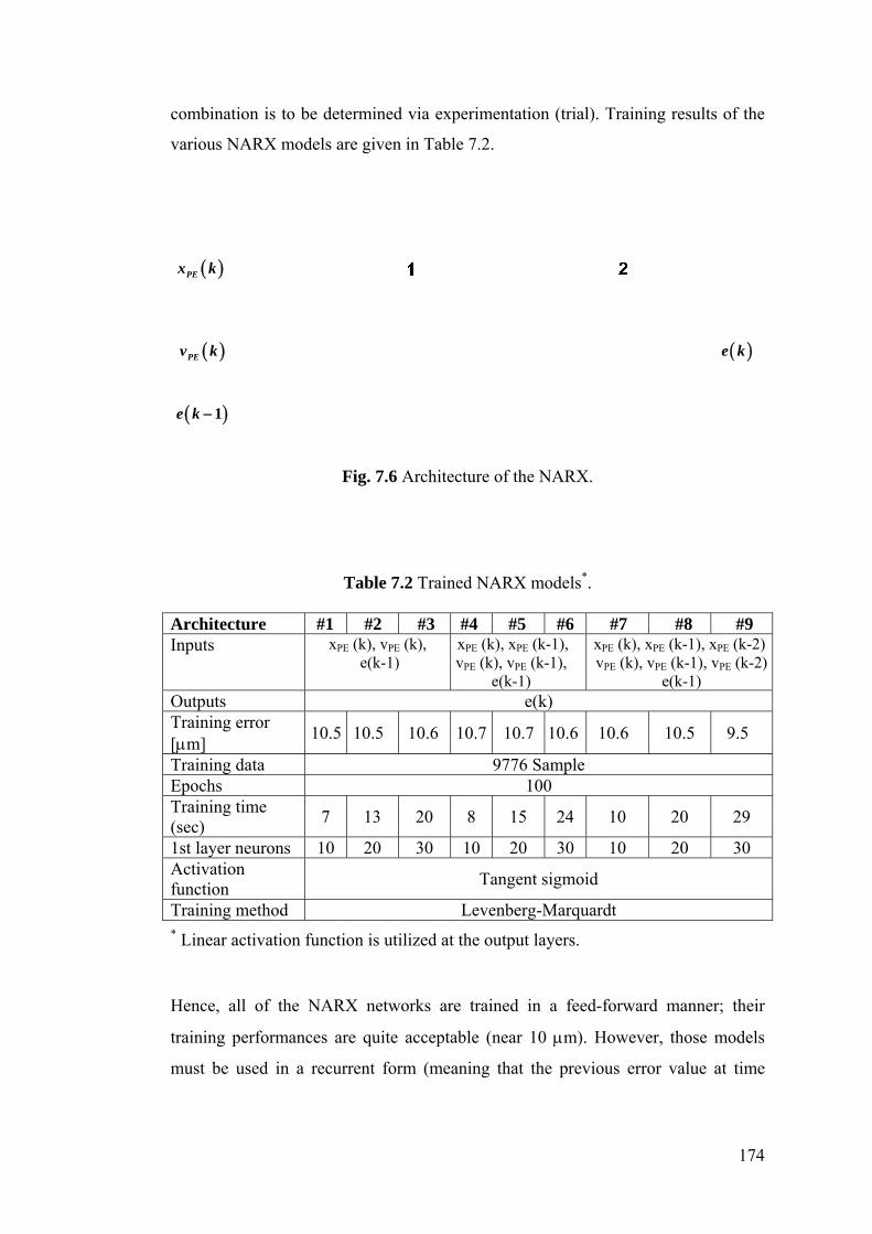
174

combination is to be determined via experimentation (trial). Training results of the

various NARX models are given in Table 7.2.

( )e k

( )e k 1−

( )PEv k

( )PEx k

Fig. 7.6 Architecture of the NARX.

Table 7.2 Trained NARX models*.

Architecture #1 #2 #3 #4 #5 #6 #7 #8 #9 Inputs xPE (k), vPE (k),

e(k-1) xPE (k), xPE (k-1),

vPE (k), vPE (k-1), e(k-1)

xPE (k), xPE (k-1), xPE (k-2) vPE (k), vPE (k-1), vPE (k-2)

e(k-1) Outputs e(k) Training error [μm] 10.5 10.5 10.6 10.7 10.7 10.6 10.6 10.5 9.5

Training data 9776 Sample Epochs 100 Training time (sec) 7 13 20 8 15 24 10 20 29

1st layer neurons 10 20 30 10 20 30 10 20 30 Activation function Tangent sigmoid

Training method Levenberg-Marquardt * Linear activation function is utilized at the output layers.

Hence, all of the NARX networks are trained in a feed-forward manner; their

training performances are quite acceptable (near 10 μm). However, those models

must be used in a recurrent form (meaning that the previous error value at time

175

index k-1must come from the network model itself). Therefore, the next step is to

feed back the output of the NARX network, which is delayed one sampling period,

to its first layer as could be seen from Fig. 7.7.

Following that, these recurrent networks, which are referred to as NOE models, are

additionally trained via RTRL algorithm. As could be seen from Table 7.3, the

networks could be trained without any problem in a recurrent form provided that the

initial weight values are taken from the NARX model. It is seen that NOE #9 has

the smallest training error (31.1 μm). Note that this particular network could not

track the sinusoidal waveform superimposed onto the error signal due to the

eccentricity of the drum as this situation can be easily seen from Fig. 7.8. For that

reason, the regression vector should be updated as shown below in order to capture

the drum eccentricity effects on the position error:

( ) ( ) ( ) ( ) ( ) ( ) ( )

( )( ) ( )( )[ , 1 ,, 2 , , 1 , 2 ,

cos , ]PE PE PE PE PE PE

TPE PE

k x k x k x k v k v k v k

k sin k

ϕ

θ θ

= − − − −

(7.3)

Table 7.3 Trained NOE models*.

Architecture #1 #2 #3 #4 #5 #6 #7 #8 #9 Inputs xPE (k), vPE

(k) xPE (k), xPE (k-1), vPE (k), vPE (k-1)

xPE (k), xPE (k-1), xPE (k-2), vPE (k), vPE (k-1), vPE (k-2)

Outputs e(k) Training error in (μm) 47 42.2 38.2 50.6 39.4 39.2 53.1 38.6 31.1

Training data 9776 Sample Epochs 10 Training time (sec) 390 403 410 392 411 413 399 414 428 1st layer neurons 10 20 30 10 20 30 10 20 30 Activation function Tangent sigmoid Training method RTRL * Linear activation function is utilized at the output layers.

176

( )e k

( )e k 1−

( )PEx k

( )PEv k

Δ

Fig. 7.7 Architecture of the NOE.

0 50 100 150 200 250 300 350 400 450 500-2.5

-2

-1.5

-1

-0.5

0

0.5

Time [sec]

Posi

tion

Erro

r [m

m]

ErrorNOE #9

Fig. 7.8 Training performance of the NOE #9.

Maintaining the train operation of the network NOE#9 with using this new

regression vector, a new network, called NOE #10, is obtained as shown in Fig.7.9.

The training error now decreases to 16.6 μm where the training performance of this

new network in time domain is given in Fig. 7.10. As can be seen from the first

inset in Fig. 7.10, NOE #10 is now able to capture the slippage dynamics due to

eccentricity of the drum. However, there is an important drift problem if one looks

into the second inset in Fig. 7.10. Although the drum velocity is exactly zero

177

(meaning that the position error must be constant at these time intervals), the

outputs of the NOE models are not constant but do drift in time. Therefore, the

black-box modeling approaches are not sufficient to predict the position error of the

cable-drum mechanism accurately. In any way, one needs to apply structured neural

network topology for this specific prediction task problem.

( )e k

Δ( )e k 1−

( )PEx k

( )PEv k

( )( )PE kcos θ

( )( )PE ksin θ

Fig. 7.9 Architecture of the NOE#10.

0 50 100 150 200 250 300 350 400 450 500-2.5

-2

-1.5

-1

-0.5

0

0.5

Time [sec]

Posi

tion

Erro

r [m

m]

ErrorNOE #9NOE #10

Fig. 7.10 Training performance of the NOE #9 and NOE #10.

178

7.4.2 Structured Neural Network Design

Since the prediction problem of NOE#10 is an output drift problem at zero-velocity,

one needs some auxiliary networks beside that network to make its output constant

when the drum velocity is exactly zero. For that purpose, first a specific network,

called zero region detector (ZRD), is designed to capture the velocity of the drum

near zero velocity region. The architecture of this network is given in Fig.7.11 and

the implemented mathematical functional could be given below:

1 , 0.001 0.0011,

xy

otherwise+ − ≤ ≤ +⎧

= ⎨−⎩

(7.4)

Fig. 7.11 Architecture of the ZRD network.

As could be seen from Fig. 7.11, ZRD is a two layered feed-forward network with

two hard-limit (type) neurons in the first layer and one linear neuron at the output

layer. The zero velocity range is adjusted by the bias weight values of the first layer.

Consequently, a switching network is also utilized while constructing the SNN

model. Eventually, the velocity signal is to be connected to the input of the ZRD

network to detect the low velocities. Finally, the output of the ZRD network is

179

connected to the “switch” port of the switching network in order to direct the output

of this network. The overall SNN is presented in Fig. 7.12. Note that in this

topology, it is guaranteed that when the speed of the drum is below 0.001 mm/s, the

predicted position error does not drift in time as zero input is fed to the integrator

(present at the output layer of the SNN) for this particular case.

Δ( )PEx k( )PEv k

( )( )cos PE kθ

( )( )PEsin kθ

Fig. 7.12 Structured neural network.

7.5 Results and Discussions

Up to now, the trained networks are not validated through a scenario different than

the training case. For that purpose, a validation test is performed based on a

scenario presented in Fig. 7.13. The position and velocity profile of the drum are

shown in Fig. 7.13.a for this validation scenario. On the other hand, Fig. 7.13.b

presents the measured position error for this experiment and the position error

predicted by the devised SNN. The unpredicted part of the position error, which

gradually increases in time, is shown in Fig. 7.13.c. It is found that the root-mean-

square (RMS) of the unpredicted position error (residual) is about 77 μm for this

random motion profile which lasts about 250 seconds.

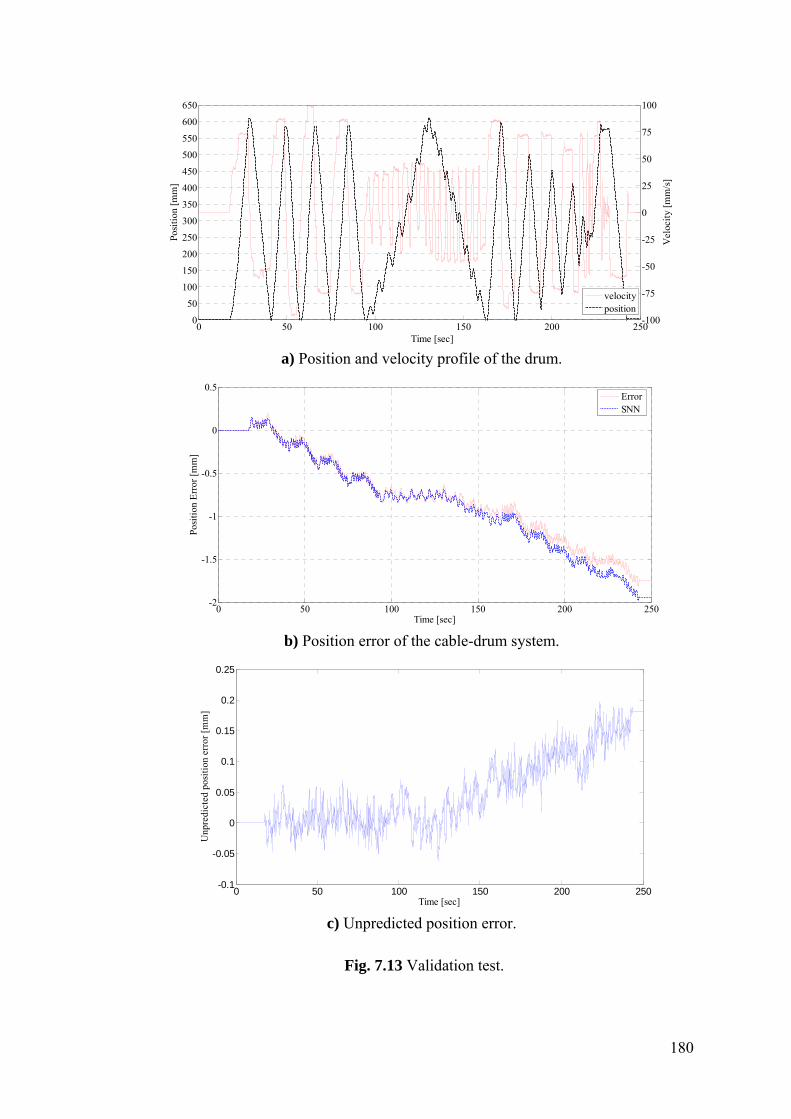
180

0

50

100

150

200

250

300

350

400

450

500

550

600

650

Time [sec]

Posi

tion

[mm

]

0 50 100 150 200 250-100

-75

-50

-25

0

25

50

75

100

Vel

ocity

[mm

/s]

velocityposition

a) Position and velocity profile of the drum.

0 50 100 150 200 250-2

-1.5

-1

-0.5

0

0.5

Time [sec]

Posi

tion

Erro

r [m

m]

ErrorSNN

b) Position error of the cable-drum system.

0 50 100 150 200 250-0.1

-0.05

0

0.05

0.1

0.15

0.2

0.25

Time [sec]

Unp

redi

cted

pos

ition

err

or [m

m]

c) Unpredicted position error.

Fig. 7.13 Validation test.

181

It is evident that to predict the slip dynamics without any error is not an easy task as

this friction based phenomenon depends on a large number of parameters. For that

reason, the developed SNN model could not capture the dynamics of the slip with

only using the position information of the drum. Furthermore, other physical

parameters (like external load on the cable) could be utilized as an input to the

network models to enhance the accuracy of the predictions. However, such

requirements would clearly hinder the practical value of the estimator and would

limit its applicability. As a practical and inexpensive solution, a beacon (or a limit

switch) could be placed at home position (HP) of the carriage to reset the overall

position error when carriage returns to this HP. With this new arrangement, Fig.

7.14.a shows the performance of the SNN using HP solution to the same validation

scenario, given in Fig. 7.14.a. Again, the unpredicted part of the position error is

presented, given in Fig. 7.14.b. The RMS of the unpredicted error is now calculated

as 29 μm. Moreover, it isobserved that the minimum- and the maximum error of the

SNN model are in the 100 μm bandwidth, which is a critical level for precision

systems, for this arbitrary validation scenario.

0 50 100 150 200 250

-0.7

-0.6

-0.5

-0.4

-0.3

-0.2

-0.1

0

0.1

0.2

Time [sec]

Posi

tion

Erro

r [m

m]

ErrorSNN

a) Position error of the cable-drum system.

182

0 50 100 150 200 250-0.1

-0.08

-0.06

-0.04

-0.02

0

0.02

0.04

0.06

0.08

0.1

Time [sec]

Unp

redi

cted

Pos

ition

Err

or [m

m]

b) Unpredicted position error.

Fig. 7.14 Validation scenario using HP approach.

7.6 Closure

This chapter has evaluated the cable-drum mechanisms as linear motion sensor for

certain machine systems. Literature survey of such systems showed that the

slippage between the cable and drum depended on many physical factors such as

eccentricity of the drum, kinematic friction coefficient between the cable and drum,

external and preload force on the cable. Furthermore, the complementary

experimental study indicated that the small fluctuations in mechanism’s speed

yielded a considerable (micro) slip at the interface. Therefore, it has been seen that

the calculation of this slippage by an analytical method was obviously unpractical.

Therefore, it is aimed to calculate this slippage via a SNN model. The work

illustrated that if the accumulated position error (drift) of the drum was reset

periodically via an absolute reference (beacon), the devised model could estimate

the position of a carriage, housing a cable-drum mechanism, with in an acceptable

error band (<100 μm).

183

CHAPTER 8

CONCLUSIONS AND RECOMMENDATIONS

8.1 Significance of this Research

This work seeks the solution of rather difficult problem: system modeling and

identification of some nonlinear systems from mechanical engineering domain

using ANNs. It has been seen that using conventional neural network structures

(black-box models) was not sufficient to handle the complex dynamic behavior of

these mechanical systems. Chapter 2 has highlighted the accurate modeling and

identification capability of structured neural networks in the current state of the art.

But, it was seen that the design strategies for SNNs were either incomplete when

viewed from a general perspective. For that purpose, a general methodology

(proposed in Chapter 3) deals with how to design SNNs using the a priori

information available from the engineering knowledge. In this approach, the task is

first decomposed into subtasks and then some networks are trained (or directly

taken from the standard library) considering these subtasks. Therefore, SNNs

consist of some independent neural networks cooperating with each other in order

to model the behavior of system within the framework of prediction/estimation. It is

important to note that each independent network operates as a single module and

works in its own domain to full its assigned task. In the corresponding chapters, a

unique SNN was designed for each of the nonlinear mechanical systems under

study (i.e. timing-belt drive, cable-drum mechanism and hydraulic systems). The

experimental results provided the accurate verification of the devised SNNs under

challenging conditions. It was observed that that the modular design of neural

network has enhanced the training and generalization performances of these ANNs,

184

resulting in a more robust and reliable network models. Consequently, this

dissertation has demonstrated the great potential of using SNNs to estimate or

predict successfully the (unavailable) states of the mechanical systems with their

complex nonlinearities such as dead-zone, backlash, hysteresis and friction

elements. Therefore, the contributions of this thesis work could be summarized as

follows:

1. A design methodology of SNNs for modeling and identification of nonlinear

systems is almost completed. The proposed modeling technique will be of

primary importance since the SNNs, which are developed especially using a

sketchy guidance of a priori knowledge on the investigated process, will have a

great capability of capturing the unaccounted system dynamics which is not

taken into consideration during the mathematical modeling of the process.

Furthermore, these a priori information-based neural networks have another

significant characteristic of modularization in which some parts of the models

could be added, deleted or changed in order to identify similar systems

accurately.

2. A new entropy based pruning algorithm is proposed to delete the redundant

neurons in a network and explained in Chapter 3 in a detailed manner. Through

some benchmark systems (taken from the literature), it has been demonstrated

that the technique effectively prunes the redundant units (neurons) of a

complex network.

3. Chapter 4 concentrates on devising a feasible SNN model for the position

estimation of a carriage system which is driven by a timing-belt mechanism.

Only the indirect measurements of the carriage system, recorded via low-cost

rotary encoder, is utilized in the designed estimator. Model validation tests

show that the devised SNN could estimate all the transmission errors of the

drive system, which are the backlash in the gear-box of the motor, friction and

hysteresis phenomenon between the teeth of the motor pinion and belt pinion,

in an acceptable error band (about 30 μm). Therefore, this model could be

185

effectively used as an open-loop controller for compensating the position error

of timing-belt driven mechanical systems.

4. In Chapter 5, an SRNN is proposed to predict the pressure dynamics for servo-

valve controlled hydraulic systems quite acceptable (±5 bars) in relatively long-

term periods (50000 steps). The major contribution of this study is the

design/development of a SNN topology which is tailored to capture the long-

term pressure dynamics of electro-hydraulic servo-systems which is inherently

nonlinear in nature. Searching the current literature comprehensively, there is

not any ANN models (whether generic or structured) that can predict the long-

term chamber pressures of such systems. It is shown that utilizing an

experimental data, one can easily adjust the weights of this particular SRNN to

characterize pressure dynamics of a servo-controlled hydraulic system.

5. Chapter 6 illustrates the design of another SRNN to predict the chamber

pressures of a speed variable pump controlled hydraulic system in extended

time periods. It is observed that the devised model could be used in a successful

manner to predict the pressure in one chamber with a RMS error about 1-2

(bars) when the pressure value of the opposite chamber is available. Therefore,

the main contribution of this study is to reduce the number of pressure sensors

in such hydraulic systems since the use of pressure sensors adds to the cost,

size, weight and complexity of the overall system. Especially, if the studies of

Guo et al. (2008) and Pi and Wang (2011), in which they are using 12 pressure

sensors for controlling a 6-DOF parallel mechanism based robotic

manipulators, are taken into consideration, the contribution of the study will be

seen more clearly.

6. A particular SNN is devised as a feasible position estimation scheme for cable-

drum mechanisms in Chapter 7. The experimental results of the work indicate

that the proposed model (SNN) could compensate the position error of the

mechanism within the 100 μm error band. Therefore, such a simple mechanism

186

with the devised SNN model could be used as a linear motion sensor for low-

end (and cost sensitive) machine systems.

8.2 Recommendations

Although this research has proposed a general methodology for devising SNNs in a

systematic fashion, all stages were not completely applied while designing neural

network models for the investigated mechanical systems. That is, the devised SNNs

were left in a modular form and no further attempt was made to optimize the SNNs

(which happens to be the most essential step for hardware implementation of such

networks). The SNNs were not converted into a generic (standard) type network

models since it is desired to preserve the physical structure of the network.

Otherwise, the modularity feature of the SNNs will disappear. Hence, it will also

reduce the utilization of these models for the modeling of other similar systems. For

instance, despite the fact that the presented study in Chapter 5 concentrates on an

EHSS with zero-lapped servo-valve, other hydraulic system topologies employing

different types of servo-valves (e.g. under lapped or over lapped) can also be easily

accommodated by the presented SRNN due to its modular structure. Provided that

specialized flow-rate NN models are designed to mimic the dynamics of the above

mentioned servo-valves (via the presented approach in this work), one can devise a

specialized SRNN conveniently by simply replacing the existing flow-rate networks

with the new ones in a modular fashion without altering the other parts of the

network. In any way, there exists an opportunity to blend and prune the network

modules to create a generic recurrent network topology. Research efforts on this

issue will be go on. The other recommendations and future work of the thesis work

could be stated as follows:

1. All the stages of the proposed SNN methodology are now applied manually.

However, an automation of the whole design process by some expert systems

will have a great impression in the research field of nonlinear system

identification and modeling.

187

2. The proposed (entropy based) pruning algorithm deletes only the redundant

neurons in a network. Although pruning a neuron rather than its weight is more

effective from the reduction of computation burden point on the hardware

platform, remaining excessive weight values should also be removed.

Therefore, other well-known pruning methods such as saliency- (OBD, OBS,

unit-OBS, mw-OBS), perturbation- or evolutionary based algorithms could be

further utilized as a part of the proposed method.

3. It is known that model predictive controllers require the future values of the

predicted plant outputs while reducing the difference (error) between the

command tracking signal and the predicted values of the process. Hence, the

networks, which are especially devised for the long-term prediction tasks in this

thesis work, could be used to realize more effective predictive controllers as a

future work.

4. In Chapter 5, the leakage effects in the hydraulic actuator was neglected to

avoid the design of a cross-coupled model (i.e. the outputs of the model must

feed each other) when applying the SNN methodology. No doubt, this cross-

coupled model will yield a more complex SRNN model. Considering the other

factors beside the leakage such as temperature and viscosity, much more

complex SRNN models could be devised in the future.

5. This thesis has not dealt with the hardware implementation of the devised

SNNs. As a future study, the well-performed networks could be implemented

on cost effective platforms such as FPGAs, FPAAs and GPUs in order to

produce customized network models for application specific systems (a

network system on a chip).

188

REFERENCES 1. Aadaleesan, P., Miglan, N., Sharma, R. and Saha, P. 2008. Nonlinear system

identification using Wiener type Laguerre-Wavelet network model. Chemical Engineering Science, 63, 3932-3941.

2. Abrate, S. 1992. Vibrations of belts and belt drives. Mechanism and Machine

Theory, 27(6), 645–659. 3. Agarwal, M. 1997. Combining neural and conventional paradigms for

modeling, prediction and control. International Journal of Systems Science, 28(1), 65-81.

4. Aguirre, L.A., Coelho, M.C.S. and Correa, M.V. 2005. On the interpretation

and practice of dynamical differences between Hammerstein and Wiener models. Control Theory and Applications, 152 (4), 349-356.

5. Akiyema, Y., Yamashita A., Kajiura M., Anzai Y. and Aiso H. 1991. The

Gaussian Machine: A Stochastic Neural Network for Solving Assignment Problems. Journal of Neural Network Computing, 3, 43-51.

6. Al-Ghoneim, K. and Kumar, V. 1995. Learning ranks with neural networks.

In Applications and Science of Artificial Neural Networks, 2492, 446-464. 7. Ankenbrand, T. and Tomassini, M. 1996. Forecasting financial multivariate

time series with neural networks. International Symposium on Neuro-Fuzzy Systems, 95-101.

8. Ardalani-Farsa, M. and Zolfaghari, S. 2010. Chaotic time series prediction

with residual analysis method using hybrid Elman-NARX neural networks. Neurocomputing, 73, 2540-2553.

9. Artmeyer, M., Lorenz, R.D. and DeVries, M.F. 1995. Process identification

and modeling using structured topologies of artificial neural networks. In Proceedings of CIRP/VDI Conference, pp. 127-140.

10. Astrom, K.J. and Canudas-De-Wit, C. 2008. Revisiting the LuGre model.

IEEE Control Systems Magazine, 28(6), 101-114.

189

11. Atuonwu, J.C., Cao, Y., Rangaiah, G.P. and Tade, M.O. 2010. Identification and predictive control of a multistage evaporator. Control Engineering Practice, 18, 1418-1428.

12. Auda, G. and Kamel, M. 1998. Modular neural network classifiers: a

comparative study. Journal of Intelligent and Robotic Systems, 21, 117-129. 13. Ayalew, B. and Kulakowski, B. 2005. Modeling supply and return dynamics

for an electrohydraulic actuation system. IISA Transactions, 44, pp. 329-343. 14. Azaam, F. 2000. Biologically Inspired Modular Neural Networks. Ph.D.

thesis, Virginia Polytechic Institute. 15. Bade, S.L. and Hutchings, B.L. 1994. FPGA-Based Stochastic Neural

Networks – Implementation. IEEE Workshop on FPGAs for Custom Computing Machines Workshop, Napa, pp. 189-198.

16. Baltersee, J. and Chambers, J.A. 1998. Nonlinear adaptive prediction of

speech with a pipelined recurrent network. IEEE Trans. Signal Process., 46(8), 2207-2216.

17. Banakar, A. and Azeem, M.F. 2012. Local recurrent sigmoidal-wavelet

neurons in feed-forward neural network for forecasting of dynamic systems: Theory. Applied Soft Computing, 12, 1187-1200.

18. Barbosa, B.H.G., Aguirre, L.A., Martinez, C.B. and Braga, A.P. 2011. Black

and gray-box identification of a hydraulic pumping system. IEEE Transactions on Control Systems Technology, 19(2), 398-406.

19. Barbounis, T.G. and Theocharis, J.B. 2007. Locally recurrent neural networks

for wind speed prediction using spatial correlation. Information Sciences, 177, 5775-5797.

20. Bartfai, G. 1994. Hierarchical clustering with ART neural networks. World

Congress on Computational Intelligence, 2, 940-944. 21. Baruch, I.S., Beltran, R., Garrido, R. and Nenkova, B. 2005. A recurrent

neural multi-model for mechanical systems dynamics compensation. Cybernetics and Information Technologies, 5(2), 21-31.

22. Baruch, I.S., Flores, J.M., Nava R.F., Ramirez P, I.R. and Nenkova, B. 2002.

An advanced neural network topology and learning, applied for identification and control of a DC motor. In Proceedings of IEEE Symposium on Intelligent Systems,1, pp. 289-295.

23. Baser, O. and Konukseven, E.I. 2010. Theoretical and Experimental

Determination of Capstan Drive Slip Error. Mechanism and Machine Theory, 45, 815-827.

190

24. Battiti, R. and Colla, A. 1994. Democracy in neural nets: Voting schemes for classification. Neural Networks, 7(4), 691-707.

25. Baum, E.B. 1991. Neural net algorithms that learn in polynomial time from

examples and queries. IEEE Trans. on Neural Networks, 2 (1), 5-19. 26. Baum, E.B. and Haussler, D. 1989. What size gives valide generalization.

Neural Computing, 1, 151-160. 27. Bechtel, S.E, Vohra, S., Jacob, K.I. and Carlson, C.D. 2000. The Stretching

and Slipping of Belts and Fibers on Pulleys. ASME J. of Applied Mechanics, 67, 197-206.

28. Bengio, Y., Simard, P. and Frasconi, P. 1994. Learning long-term

dependencies with gradient descent is difficult. IEEE Transactions on Neural Networks 5, 157-166.

29. Billings, S.A. and Zhu, Q.M. 1994. Nonlinear model validation using

correlation tests. International Journal of Control, 60, 1107-1120. 30. Blum, A.L. and Riyest, R.L. 1992. Training a 3-node neural network is NP-

complete. Neural Networks, 5 (1), 117-127. 31. Bohte, S.M., Poutr´e, H.L. and Kok, J.N. 2002. Error-backpropagation in

temporally encoded networks of spiking neurons. Neurocomputing, 48, 17–37.

32. Caliskan, H. 2009. Modeling and Experimental Evaluation of Variable Speed

Pump and Valve Controlled Hydraulic Servo Drives. Ms. thesis at Middle East Technical University, Ankara, Turkey.

33. Cernansky, M. 2009. Training Recurrant Neural Network Using Multistream

Extended Kalman Filter on Multicore Processor and Cuda Enabled Graphic Processor Unit. International Conference on Artificial Neural Networks, 1, pp. 381-390.

34. Chan L. and Li, Y. 2000. Dynamic Modelling and Time Series Prediction by

Incremental Growth of Lateral Delay Neural Networks. IEEE Symposium on Combinations of Evolutionary Computation and Neural Networks, 216-223.

35. Che, S., Boyer, M., Meng, J., Tarjan, D., Sheaffer, J.W. and Skadron, K.

2008. A performance study of general-purpose applications on graphics procesors using CUDA. J. Parallel Distrib. Comput., 68, 1370-1380.

36. Chen, S., Wang, X.X. and Harris, C.J. 2008. NARX Based Nonlinear System

Identification Using Orthogonal Least Squares Basis Hunting. IEEE Transactions on Control Systems Technology, 16 (1), 78-84.

191

37. Chi, C.W., Hsia, S.T.C., Tseng, H.C. 1997. Adaptive aggregation of modular fuzzy control. IEEE International Conference on Systems, Man, and Cybernetics, Orlando, Florida.

38. Coelho, L.S., Pessoa, M.W. 2009. Nonlinear identification using a B-spline

neural network and chaotic immune approaches. Mechanical Systems and Signal Processing, 23, 2418-2434.

39. Corwin, E., Greni, S., Logar, A. and Whitehead, K. 1994. A multi-stage

neural network classifier. World Congress on Computational Intelligence, 3, 198-203.

40. Cun, Y.L., Denker, J.S. and Solla, S.A. 1990. Optimal brain damage. In

Proceedings of the Neural Information Processing Systems, 2, pp. 598–605. 41. Dang, X. and Tan, Y. 2007. RBF neural networks hysteresis modeling for

piezoceramic actuator using hybrid model. Mechanical Systems and Signaş Processing, 21, 430-440.

42. Dempster, A.P., Laird, N.M. and Rubin, D.B. 1977. Maximum likelihood

from incomplete data via the EM algorithm. Journal of the Royal Statistical Society, 39 (1), 1-38.

43. Deng, L., and Tan, Y. 2008. Diagonal recurrent neural network with modified

backlash operators for modeling of rate-dependent hysteresis in piezoelectric actuators. Sensors and Actuators A: Physical, 148, 259-270.

44. Dolen, M. 2000. Modeling and Estimation by Structured Neural Networks for

CNC Machine Tools. Ph.D. thesis, University of Wisconsin, USA. 45. Dolen, M. and Lorenz, R.D. 2002. General Methodologies for Neural

Network Programming. Smart Engineering System Design, 4, 63-73. 46. Dong, P., Bilbro, G.L. and Chow, M. 2006. Implementation of artificial

neural network for real time applications using field programmable analog arrays. International Joint Conf. on Neural Networks, Vancouver, Canada, pp. 1518-1524.

47. Endisch, C., Brache, M., Endish, P., Schroder, D. and Kennel, R. 2009.

Identification of Mechatronic Systems with Dynamic Neural Networks using Prior Knowledge. In Proceedings of the World Congress on Engineering and Computer Science, pp. 859-865.

48. Engelbrecht, A.P. 2001. A new pruning heuristic based on variance analysis

of sensitivity information. IEEE Trans. Neural Networks, 12, 1386–1399. 49. Euler, M.L. 1762. Remarques sur l’effect du Frottement dans l’equilibre

(Remarks on the effect of friction in balance). Mém. Acad. Sci., 265-278.

192

50. Fahlman, S.E. and Lebiere, C. 1990. The cascade-correlation learning

architecture, in: D.S. Touretzky (Ed.). Advances in Neural Information Processing, 2, 524–532.

51. Fawcett, J.N. 1981. Chain and Belt Drives – A Review. Shock and Vibration

Digest, 13(5), 5-12. 52. Finnoff, W., Hergert, F., and Zimmermann, H.G. 1993. Improving model

selection by nonconvergent methods. Neural Networks, 6, 771-783. 53. Firbank, T.C. 1970. Mechanics of the Belt Drive. Int. J. of Mech. Sci., 12,

1053-1063. 54. Garcia, P., Briz, F., Raca, D. and Lorenz, R.D. 2007. Saliency-tracking –

based sensorless control of AC machines using structured neural networks. IEEE Transactions on Industry Applications, 43(1), 77-86.

55. Ge, H., Qian, F., Liang, Y., Du, W. and Wang, L. 2008. Identification and

control of nonlinear systems by a dissimilation particle swarm optimization-based Elman neural network. Nonlinear Analysis: Real World Applications, 9, 1345-1360.

56. Gerbert, G.G. 1996. Belt Slip – A Unified Approach. ASME J. of Mech.

Design, 118, 432-438. 57. Gerbert, G.G. 1999. Traction Belt Mechanics, Chapters 7-10, Chalmers Univ.

of Tech. Press, Sweden. 58. German, S., Bienenstock, E. and Doursat, R. 1992. Neural networks and the

bias/variance dilemma. Neural Computation 4(1), 1-58. 59. Girolami, M. and Gyfe, C. 1997. Extraction of independent signal sources

using a deflationary exploratory projection pursuit network with lateral inhibition. IEE Proceedings on Vision, Image and Signal, 144 (5), 299-306.

60. Girosi, F., Jones, M. and Poggio, T. 1995. Regularization theory and neural

network architectures. Neural Computing, 7, 219–269. 61. Goh, S.L. and Mandic, D.P. 2005. Nonlinear adaptive prediction of complex-

valued signals by complex-valued PRNN. IEEE Transactions on Signal Processing, 53(5), 1827-1836.

62. Goldberg, D.E. 1989. Genetic Algorithms in Search, Optimization and

Machine Learning. Addison Wesley.

193

63. Gonzales-Olvera, M.A. and Tang, Y. 2007. A new recurrent neurofuzzy network for identification of dynamic systems. Fuzzy Sets and Systems, 158, 1023-1035.

64. Grashof, B.G. 1883. Theoretische Machinenlehre, Band 2, Leopold Voss,

Hamburg. 65. Guan, C. and Pan, S. 2008. Adaptive sliding mode control of electro-

hydraulic system with nonlinear unknown parameters. Control Engineering Practice, 16, 1275-1284.

66. Guan, G.Q. and Chen, J.Q. 2005. Building optimal back-propogation trained

neural networks for firm bankruption predictions. In Proceedings of the Information Resources Management Association International Conference, pp. 449- 452.

67. Guo, H., Liu, Y., Liu, G. and Li, H. 2008. Cascade control of hydraulically

driven 6-DOF parallel robot manipulator based on a sliding mode. Control Engineering Practice, 16, 1055-1068.

68. Hace, A., Jezernik, K. and Sabanovic, A. 2005. Improved design of VSS

Controller for a linear belt-driven servomechanism. IEEE/ASME Transactions on Mechatronics, 10(4), 385–390.

69. Hametner, C. and Jakubek, S. 2011. Nonlinear identification with local model

networks using GTLS techniques and equality constraints. IEEE Transactions on Neural Networks, 22(9), 1406-1418.

70. Hamming, R.W. 1986. Coding and Information Theory, Second edition. New

Jersey: Prentice Hall. 71. Hamrouni, L., Kherallah, M. and Alimi, A.M. 2011. Textile plant modeling

using recurrent neural networks. In Proceedings of the IEEE International Conference on Systems, Man, and Cybernetics, pp. 1580-1584.

72. Han, X., Xie, W.F., Fu,Z. and Luo, W. 2011. Nonlinear systems identification

using dynamic multi-time scale neural networks. Neurocomputing, 74, 3428-3439.

73. Han, Z., Yingrong, L. and Qian, L. 2006. MW-OBS: an improved pruning

method for topology design of neural networks. Tsinghua Science and Technology, 11, 307-312.

74. Hassibi, B. and Stork, D.G. 1992. Second-order derivatives for network

pruning: optimal brain surgeon. In Proceedings of the Neural Information Processing Systems, 5, pp. 164–171.

194

75. Hassibi, B., Stork, D.G. and Wolff, G. 1993. Optimal brain surgeon and general network pruning. In Proceedings of IEEE International Conference on Neural Networks, pp. 293–299.

76. Haykin, S. and Li, X.B. 1995. Detection of signals in chaos. In Proceedings of

the IEEE 83(1), 95-122. 77. He, S. and Sepehri, N. 1999. Modeling and prediction of hydraulic servo

actuators with neural networks. In Proceedings of the American Control Conference, San Diego, California, pp. 3708-3712.

78. He, X. and Asada, H. 1993. A new method for identifying orders of input-

output models for nonlinear dynamical systems. In Proceedings of American Control Conference, San Francisco, USA, pp. 2520-2523.

79. Heaton, J. 2008. Introduction to Neural Networks with Java, 2nd edition.

Heaton Research Inc. 80. Hebb, D.O. 1949. The organization of behavior. New York: Wiley & Sons. 81. Hecht-Nielsen, R. 1987. Counterpropagation networks. Applied Optimization,

26(23), 4979-4984. 82. Helbig, A., 2002. Injection molding machine with electric-hydrostatic drives.

3rd International Fluid Power colloquium, 1, 67-81. 83. Helduser, S., 2003. Improved energy efficiency in plastic injection molding

machines. 8th Scandinavian International Conference on Fluid Power, Tampere, Finland.

84. Hikawa, H. 1999. Frequency Based Multilayer Neural Network with on chip

learning and Enhanced Neuron characteristics. IEEE Transactions on Neural Networks, 10(3), 545-553.

85. Hikawa, H. 2003. A New Digital Pulse-Mode Neuron with Adjustable

Activation Function. IEEE Transactions on Neural Networks, 14(1), 236-242. 86. Hinton, G.E., Sejnowski, T.J. and Ackley, D.H. 1984. Boltzmann machines:

constraint satisfaction network that learn. Carnegie Mellon University technical report, CMU-CS-84-119.

87. Hintz, C., Rau, M. and Schroder, D. 2000. Identification of a nonlinear multi

stand rolling system by a structured recurrent neural network. In Proceedings of IEEE Industry Applications Conference, pp. 1121–1128.

88. Hong, X. and Chen, S. 2011. Modeling of complex-valued Wiener systems

using B-spline neural network. IEEE Transactions on Neural Networks, 22(5), 818-825.

195

89. Hunt, K.J., Sbarbaro, D., Zbikowski, R. and Gawthrop, P.J. 1992. Neural networks for control systems- a survey. Automatica, 28, 1083-1112.

90. Ishikawa, M. 1996. Structural learning with forgetting. Neural Networks, 9,

509–521. 91. Iwata, A., Nagasaka, Y. and Suzumura, N. 1990. Data compression of the

ECG using neural network for digital Holter monitor. IEEE Engineering in Medicine and Biology Magazine, 9 (3), 53-57.

92. Jacobs, R.A. 1995. Methods of combining expert’s probability assessments.

Neural Computation, 7, 867-888. 93. Jang, H. Park, A. and Jung, K. 2008. Neural Network Implementation using

CUDA and OpenMP. IEEE Digital Image Computing: Techniques and Applications, DOI: 10.1109/DICTA.2008.82, 155- 161.

94. Januszewski, M. and Kostur, M. 2010. Accelerating numerical solution of

stochastic differential equations with CUDA. Computer Physics Communications, 181, 183-188.

95. Jelali, M. and Kroll, A. 2003. Hydraulic Servo-systems Modelling,

Identification and Control. London: Springer. 96. Johansen, T.A. and Foss, B.A. 1995. Identification of non-linear system

structure and parameters using regime decomposition. Automatica, 31, 321-326.

97. Johansen, T.A. and Foss, B.A. 1997. Operating regime based process

modeling and identification. Computers and Chemical Engineering, 21, 159-176.

98. Johnson, K.L. 1985. Contact Mechanics, Cambridge Univ. Press, London. 99. Jordan, M.I. and Jacobs, R.A. 1994. Hierarchical mixture of experts and EM

algorithm. Neural Computation, 6, 181-214. 100. Juang, C.F. and Hsieh, C.D. 2010. Alocally recurrent fuzzy neural network

with support vector regression for dynamic-system modeling. IEEE Transactions on Fuzzy Systems, 18(2), 261- 273.

101. Kaddissi, C., Kenne, J.P. and Saad, M. 2007. Identification and real-time

control of an electrohydraulic servo system based on nonlinear backstepping. IEEE/ASME Transactions on Mechatronics 12(1), 12-22.

102. Kaddissi, C., Kenne, J.P. and Saad, M. 2011. Indirect adaptive control of an

electrohydraulic servo system based on nonlinear backstepping. IEEE/ASME Transactions on Mechatronics, 16(6), 1171-1177.

196

103. Kagotani, M., Ueda, H. and Koyama, T. 2001. Transmission error in helical timing belt drives. Transactions of the ASME, 123, 104-110.

104. Kang, R., Jiao, Z., Wu, S., Shang, Y., and Mare, J.C. 2008. The nonlinear

accuracy model of electro-hydrostatic actuator. IEEE Conference on Robotics, Automation and Mechatronics, Chengdu, China, pp. 107-111.

105. Karnin, E.D. 1990. A simple procedure for pruning back-propagation trained

neural networks. IEEE Trans. Neural Networks, 1, 239–242. 106. Karpenko, M. and Sepehri, N. 2010. On quantitative feedback design for

robust position control of hydraulic actuators. Control Engineering Practice 18, 289-299.

107. Kautz, T.O. 1993. Cable extension linear position transducer. U.S. Patent 5

236 144. 108. Kilic, E. 2007. Novel Position Measurement and Estimation Methods for

CNC Machine Systems. M.Sc. Thesis, Middle East Technical University – Ankara, Turkey.

109. Kilic, E., Dolen, M. and Koku, A.B. 2011. Experimental Evaluation of Cable-

Drum Systems as Linear Motion Sensors. In Proceedings of IEEE International Conference on Mechatronics, Turkey, 666-671.

110. Kilic, E., Dolen, M., Koku, A.B. and Dogruer, C.U. 2007. Novel position

estimators for timing belt drives. Journal of Automation, Mobile Robotics and Intelligent Systems, 1(2), 55-61.

111. Kim, K. and Park, J. 1993. Application of hierarchical neural networks to

fault diagnosis of power systems. International Journal on Electrical Power and Energy System, 15(2), 65-70.

112. King, S.-Y. and Hwang, J.-N. 1989. Neural network architectures for robotic

applications. IEEE Transactions on Robotics and Automation, 5 (5), 641-657).

113. Kiong, L.C, Rajeswari, M. and Rao, M.V.C. 2003. Nonlinear dynamic system

identification and control via constructivism inspired neural network. Applied Soft Computing, 3, 237-257.

114. Kirkpatrick, S., Gelatt, C.D. and Vecchi, M.P. 1983. Optimization by

simulated annealing. Science, 220, 671-680. 115. Kolen, J.F. and Kremer, S.C. 2001. A Field Guide to Dynamical Recurrent

Networks. New York: IEEE Press.

197

116. Kong, L. and Parker, R.G. 2005. Microslip friction in flat belt drives. Proc. IMechE Mechanical Engineering Science., 219, 1097-1106.

117. Kong, L. and Parker, R.G. 2006. Mechanics and Sliding Friction in Belt

Drives with Pulley Grooves. ASME J. of Mech. Design, 128, 494-502. 118. Krips, M., Lammert, T. and Kummert, A. 2002. FPGA Implementation of a

Neural Network for a Real-Time Hand Tracking System. In proceedings of the First IEEE International Workshop on Electronic Design, Test and Applications.

119. Kulkarni, A.S. and El-Sharkawi, M.A. 2001. Intelligent precision position

control of elastic drive systems. IEEE Trans. on Energy Conv., 16 (1), 26-31. 120. Kurkova, V. 1991. Kolmogorov’s theorem is relevant. Neural Computations,

3(4), 617-622. 121. Kwan, H.K. 1992. Simple sigmoid like activation function suitable for digital

hardware implementation. Electronic Letters , 28, 1379 – 1380. 122. Kwok, T. and Yeung, D. 1997. Constructive algorithms for structure learning

in feedforward neural networks for regression problems. IEEE Trans. Neural Networks, 3, 630–645.

123. Lawrynczuk, M. 2010. Training of neural models for predictive control.

Neurocomputing, 73, 1332-1343. 124. Lazar, M. and Pastravanu, O. 2002. A neural predictive controller for non-

linear systems. Mathematics and Computers in Simulation, 60, 315-324. 125. Leamy, M.J. and Wasfy, T.M. 2002. Analysis of Belt-Drive Mechanics using

a Creep-Rate Dependent Friction Law. ASME J. of App. Mechanics, 69, 763-771.

126. LeCun, Y., Boser, B., Denker, J., Henderson, D., Howard, R., Hubbard, W.

and Jackel, L. 1989. Backpropagation applied to handwritten zip code recognition. Neural Computation, 1, 541-551.

127. Lemma, D.T., Ramasamy, M. and Shuhaimi, M 2010. System identification

using orthonormal basis filters. Journal of Applied Sciences 10(21), 2516-2522.

128. Li, C.J. 1995. Mechanical system modeling using recurrent neural networks

via quasi-Newton learning methods. Applied Mathematical Modelling, 19(7), 421-428.

198

129. Li, W. and Rehani, M. 1996. Modeling and control of a belt-drive positioning table. In Proceedings of the 22nd IEEE International Conference of Industrial Electronics, Taipei, 1996, pp. 1984–1989.

130. Liberati, M., Beghi, A., Mezzalira, S. and Peron, S. 2004. Grey-box

Modelling of a Motorcycle Shock Absorver. Conference on Decision and Control, 755- 760.

131. Lien, J.P., York, A., Fang, T. and Buckner, G.D. 2010. Modeling

piezoelectric actuators with hysteretic recurrent neural networks. Sensors and Actuators A, 163, 516-525.

132. Lightbody, G., O’Reilly, P., Irwin, G.W., Kelly, K. and McCormick, J. 1997.

Neural modelling of chemical plant using MLP and B-spline networks. Control Engineering Practice, 5(11), 1501-1515.

133. Lima C.A.M, Coelho, A.L.V. and Von Zuben, F.J. 2007. Hybridizing mixture

of experts with support vector machines: Investigation into nonlinear dynamic systems identification. Information Sciences, 177, 2049-2074.

134. Lin, T., Horne, B.G and Giles, C.L. 1998. How embedded memeory in

recurrent neural network architectures helps learning long-term temporal dependencies. Neural Networks, 5, 861-868.

135. Lippmann, R. 1989. Review of neural networks for speech recognition.

Neural Computation, 1, 1-38. 136. Liu, G.P., Kadirkamanathan, V. and Billings, S.A. 1998. On-line

identification of nonlinear systems using Volterra polynomial basis function neural networks. Neural Networks 11, 1645-1657.

137. Liu, J.N.K. and Lee, R.S.T. 1999. Rainfall forecasting from multiple point

sources using neural networks. IEEE International Conference on Systems, Man, and Cybernetics, 3, 429-434.

138. Ljung, L. 1999. System Identification: Theory for the User. London: Prentice

Hall. 139. Lovrec, D., Kastrevc, M., Ulaga, S., 2008. Electro-hydraulic load sensing

with speed-controlled hydraulic supply system on forming machines. International Journal Advanced Manufacturing Technology 1, 1066-1075.

140. Lovrec, D., Ulaga, S., 2007. Pressure control in hydraulic systems with

variable or constant pumps. Experimental Techniques 31 (2), 33-41. 141. Lu, B.L. and Ito, M. 1999. Task decomposition and module combination

based on class relations: a modular neural network for pattern classification. IEEE Transactions on Neural Networks, 10(5), 1244-1256.

199

142. Macleod, C., Maxwell, G. and Muthuraman, S. 2009. Incremental growth in modular neural networks. Engineering Applications of Artificial Intelligence, 22, 660-666.

143. MacQueen, J.B. 1967. Some methods for classification and analysis of

multivariate observations. Proceedings of the 5th Berkeley Symposium on Mathematical Statistics and Probability, 281-297.

144. Maeda, Y. and Tada, T. 2003. FPGA implementation of a pulse density neural

network with learning ability using simultaneous perturbation. IEEE Transactions on Neural Networks, 14(3), 688-695.

145. Maeda, Y., Hiramatsu, T., Miyoshi, S. and Hikawa, H. 2009. Pulse Coupled

Oscillator with Learning Capability Using Simultaneous Perturbation and Its FPAA Implementation. ICROS-SICE International Joint Conference, Fukuoka, Japan, pp. 3142-3145.

146. Maher, J., Ginley, B., Rocke, P. and Morgan, F. 2006. Intrinsic Hardware

Evolution of Neural Networks in Reconfigurable Analogue and Digital Devices. IEEE Symposium on Field-Programmable Custom Computing Machines.

147. Maria, J., Menezes, P. and Baretto, G. 2008. Long-term time series prediction

with the NARX network: An empirical evaluation. Neurocomputing, 71, 3335-3343.

148. Mayergoyz, I.D. 1991. Mathematical Models of Hysteresis. NewYork:

Springer. 149. Melin, P., Mancilla, A., Lopez, M. and Mendoza, O. 2007. A hybrid modular

neural network architecture with fuzzy Sugeno integration for time series forecasting. Applied Soft Computing, 7, 1217-1226.

150. Merritt, H.E. 1967. Hydraulic Control Systems. New York: John Wiley &

Sons. 151. Michalkiewicz, J. 2012. Modified Kolmogorov’s neural network in the

identification of Hammerstein and Weiner systems. IEEE Transactions on Neural Networks and leraning Systems, 23(4), 657- 662.

152. Mihajlov, M., Nikolic, V. and Antic, D. 2002. Position control of an electro-

hydraulic servo system using sliding mode control enhanced by fuzzy PI controller. Mechanical Engineering, 1(9), 1217-1230.

153. Mirzaee, H. 2009. Long-term prediction of chaotic time series with multi-step

predictipn horizons by a neural network with Levenberg-Marquardt learning algorithm. Chaos, Solitons and Fractals 41, 1975-1979.

200

154. Moallemi, C. 1991. Classifying cells for cancer diagnosis using neural networks. IEEE Expert, 6 (6), 8-12.

155. Mohanty, A., and Yao, B. 2011. Indirect adaptive robust control of hydraulic

manipulators with accurate parameter estimates. IEEE Transactions on Control Systems Technology, 19(3), 567-575.

156. Mozer, M.C. and Smolensky, P. 1989. Skeletonization: A technique for

trimming the fat from a network via relevance assessment. In Proceedings of the Neural Information Processing Systems, 1, pp. 107–115.

157. Mustafaraj, G., Lowry, G. and Chen, J. 2011. Prediction of room temperature

and relative humidity by autoregressive linear and nonlinear neural network models for open office. Energy and Buildings, 43, 1452-1460.

158. Nageswaran, J.M., Dutt, N., Krichmar, J.L., Nicolau, A. and Veidenbaum,

A.V. 2009. A configurable simulation environment for the efficient simulation of large spiking neural networks on graphics processors. Neural Networks, 22, 791-800.

159. Narendra, K.S. and Parthasarathy, K. (1989). Neural Network and Dynamical

Syetms Part II: Identification. Report No. 8002, Yale University. 160. Narendra, K.S. and Parthasarathy, K. 1990. Identification and control of

dynamical systems using neural networks. IEEE Trans. Neural Networks, 1, 4-27.

161. Nelles, O. 2001. Nonlinear System Identification. New York: Springerlink. 162. Ni, J. and Song, Q. 2006. Dynamic pruning algorithm for multilayer

perceptron based neural control systems. Neurocomputing, 69, 2097-2111. 163. Nørgaard, M. 2000. Neural network based system identification toolbox,

Technical Report 00-E-891, Department of Automation, Technical University of Denmark.

164. Nuno-Maganda, M.A., Arias-Estrada, M., Torres-Huitzil, C. and Girau, B.

2009. Hardware Implementation of Spiking Neural Network Classifiers based on Backpropagation-based Learning Algorithms. In Proceedings of International Conference on Neural Networks, Atlanta, USA.

165. Omondi, A.R. and Rajapakse, J.C. 2006. FPGA implementations of Neural

Networks. New York: Springer. 166. Orlando, J.R., Mann, R. and Haykin S. 1990. Classification of sea-ice images

using a dual-polarized radar. IEEE Journal of Oceanic Engineering, 15 (3), 228-237.

201

167. Oyama, E., Agah, A., MacDorman, K.F., Maeda, T. and Tachi S. 2001. A modular neural network architecture for inverse kinematics model learninig. Neurocomputing, 38, 797-805.

168. Pan, Y. and Sensen, C. 2005. Modular neural networks and their applications

in exon prediction. In Advances in bioinformatics and its applications series in mathematical biology and medicine, 8, 47-61.

169. Parlos, A.G., Rais, O.T. and Atiya, A.F. 2000. Multi-step-ahead prediction

using dynamic recurrent neural networks. Neural Networks 13, 765-786. 170. Patel, A. and Dunne, J.F. 2010. NARX Neural Network Modelling of

Hydraulic Suspension Dampers for Steady-state and Variable Temperature Operation. Vehicle System Dynamics, 40 (5), 285-328.

171. Pi, Y. and Wang, X. 2011. Trajectory tracking control of a 6-DOF parallel

robot manipulator with uncertain load disturbances. Control Engineering Practice, 19, 185-193.

172. Piroddi, L. and Spinelli, W. 2003. An identification algorithm for polynomial

NARX models based on simulation error minimization. International Journal of Control, 76, 1767-1781.

173. Pukrittayakameei, A., Hagan, M., Raff, L., Bukkapatnam, S. and Komanduri,

R. 2009. A network pruning algorithm for combined function and derivative approximation. In Proceedings of International Joint Conference on Neural Networks, Atlanta, USA.

174. Qiao, J., Zhang, Y. and Han, H. 2008. Fast unit pruning algorithm for

feedforward neural network design. Applied Mathematics and Computation, 205, 622-627.

175. Ramirez-Agundis, A., Gadea-Girones, R. and Colom-Palero, R. 2008. A

hardware design of a massive-parallel, modular NN-based vector quantizer for real-time video coding. Microprocessors and Microsystems, 32, 33-44.

176. Reed, R. 1993. Pruning algorithm - a survey. IEEE Trans. Neural Networks,

5, 740-747. 177. Ren, X. and Lv, X. 2011. Identification of extended Hammerstein systems

using dynamic self-optimizing neural networks. IEEE Transactions on Neural Networks, 22(8), 1169-1179.

178. Reuter, H.B. 1995. Zur Identifikation nichtlinearer Systemmodelle mit wenig

A-priori-Informationen. Dissertation in University of Duisburg, Düsseldorf, Germany.

202

179. Rogova, G. 1994. Combining results of several neural network classifiers. Neural Networks, 7, 771-781.

180. Sato, M. and Sato, Y. 1995. Neural clustering-implementation of clustering

model using neural networks. IEEE International Conference on Systems, Man and Cybernetics, 4, 3609-3614.

181. Schenker, B. and Agarwal, M. 1998. Output prediction in systems with

backlash. IMechE, 212, 17-26. 182. Schittenkopf, C., Deco, G. and Brauer, W. 1997. Two strategies to avoid

overfitting in feedforward neural networks. Neural Networks, 10, 505–516. 183. Schrauwen, B., D’Haene, M., Verstraeten, D. and Van Campenhout, J. 2008.

Compact hardware liquid state machines on FPGA for real-time speech recognition. Neural Networks, 21, 511-523.

184. Seidl, D.R. 1996. Motion and Motor Control Using Structured Neural

Networks. Ph.D. thesis, University of Wisconsin, USA. 185. Seidl, D.R. and Lorenz, R.D. 1991. A structure by which a recurrent neural

network can approximate a nonlinear dynamic system. In Proceedings of International Joint Conference on Neural Networks, pp. 709-714.

186. Seidl, D.R. and Lorenz, R.D. 1993. One-step optimal space vector PWM

current regulation using a neural network. In Proceedings of the IEEE IAS Conference, pp. 2027-2034.

187. Seidl, D.R., Lam, S.L., Putman, J.A. and Lorenz, R.D. 1993. Neural network

identification and compensation of gear backlash hysteresis in position controlled mechanisms. In Proceedings of the IEEE IAS Conference, pp. 2027-2034.

188. Seidl, D.R., Reineking, T.L. and Lorenz, R.D. 1992. Use of neural networks

to identify and compensate for friction in precision position controlled mechanism. In Proceedings of the IEEE IAS Conference, pp. 1937-1944.

189. Sharma, S.K., Irwin, G.W., Tokhi, M.O and McLoone, S.F. 2003. Learning

soft computing strategies in a modular neural network architecture. Engineering Applications of Artificial Intelligence. 16, 395-405.

190. Sibte, S. and Abidi, R. 1996. Neural networks and child language

development: A simulation using a modular neural network architecture. In Proceedings of IEEE International Conference on Neural Networks, pp. 840-845.

203

191. Siebel, N., Bötel, J. and Sommer, G. 2009. Efficient neural network pruning during neuro-evolution. In Proceedings of International Joint Conference on Neural Networks, Atlanta, USA.

192. Sietsma, J. and Dow, R.F.J. 1991. Creating artificial neural networks that

generalize. Neural Networks, 4(1), 67-69. 193. Smith, D.P. 1998. Tribology of the Belt Driven Data Tape Cartridge.

Tribology International, 31(8), 465–477. 194. Sola, J. and Sevilla, J. 1997. Importance of input data normalization for the

application of neural networks to complex industrial problems. IEEE Transactions on Nuclear Science, 44(3), 1464-1468.

195. Sorjamaa, A., Reyhani, J.H.N., Ji, Y. and Lendasse, A. 2007. Methodology

for long-term prediction of time series. Neurocomputing 70, 2861-2869. 196. Soukoulis, C.M., Levin, K. and Grest, G.S. 1983. Irreversibility and

Metastability in Spin-Glasses. I. Ising Model. Physical Review, 28, 1495-1509.

197. Söderström, T. and Stoica, P. 1989. System Identification. Prentice Hall. 198. Sprecher, D.A. 1996. A numerical implementation of Kolmogorov’s

superpositions. Neural Networks, 9(5), 765-772. 199. Stahlberger, A. and Riedmiller, M. 1996. Fast network pruning and feature

extraction using the unit-OBS algorithm. Advances in Neural Information Processing Systems, Denver, pp. 2-5.

200. Stavrakoudis, D.G. and Theocharis, J.B. 2007. Pipelined recurrent fuzzy

neural networks for nonlinear adaptive speech prediction. IEEE Trans. Syst. Man Cybern., 37(5), 1305-1320.

201. Steinich, K.M. 2007. Cable actuated position sensor with spring located inside

the cable drum. U.S. Patent 7 263 782. 202. Stepniewski, S.E. and Keane, A.J. 1997. Pruning backpropagation neural

networks using modern stochastic optimization techniques. Neural Computing & Applications, 5, 76-98.

203. Tagliarini, G.A., Christ, J.F. and Page, E.W. 1991. Optimization using neural

networks. IEEE Transactions on Computers, 40 (12), 1347-1358. 204. Tan, C.L., Quah, T.S. and Teh, H.H. 1996. An artificial neural network that

models human decision making. Computers, 29 (3), 64-70.

204

205. Te Braake, H.A.B., Babuska, R. and Van Can, H.J.L. 1994. Fuzzy and neural models in predictive control. Journal A, 35, 44-51.

206. Tellez, F.O., Loukianov, A.G., Sanchez, E.N. and Corrochano, E.J.B. 2010.

Decentralized neural identification and control for uncertain nonlinear systems: Application to planar robot. Journal of the Franklin Institute, 347, 1015-1034.

207. Tenorio, M.F. and Lee, W.T. 1990. Self-organizing network for optimum

supervised learning. IEEE Trans. Neural Networks, 1, 100–110. 208. Thayer, W.J. 1965. Transfer function for Moog servovalves. Technical

Bulletin I03 MOOG 103, East Aura, NY, USA. 209. Tokunaga, K. and Furukawa, T. 2009. Modular network SOM. Neural

Networks, 22, 82-90. 210. Treesatayapun, C. 2010. Nonlinear discrete-time controller with unknown

systems identification based on fuzzy rules emulated network. Applied Soft Computing, 10, 390-397.

211. Tseng, H.C. and Almogahed, B. 2009. Modular neural networks with

applications to pattern profiling problems. Neurocomputing, 72, 2093-2100. 212. Tseng, H.C. and Chi, C.W. 1995. Modular intelligent control. Advances in

Fuzzy Theory and Technology III. 213. Tu, C.F. and Fort, T. 2004. A Study of Fiber–Capstan Friction. 1: Stribeck

Curves. Tribology International, 37, 701–710. 214. Tufa, L.D., Ramasamy, M., Patwardhan, S.C. and Shuhaimi, M. 2010.

Development of Box-Jenkins time series models by combining conventional and orthonormal basis filter approaches. Journal of Process Control, 20, 108-120.

215. Tumer, K. and Ghosh, J. 1996. Error correlation and error reduction in

ensemble classifiers. Connection Science, 8, 385-404. 216. Van den Hof, P., Paul, M.J., Heuberger, P. and Wahlberg, B. 2005. Modeling

and Identification with Rational Orthogonal Basis Functions. London: Springer.

217. Van Hulle, M. M. and Tollenacre, T. 1993. A modular artificial neural

network for texture processing. Neural Networks, 6(1), 7-32. 218. Waibel, A. 1989. Modular construction of time-delay neural networks for

speech recognition. Neural Computation, 1(1), 39-46.

205

219. Wang, L., Der, S. and Nasrabadi, N. 1998. Automatic target recognition using a feature-decomposition and data-decomposition modular neural network. IEEE Transactions on Image Processing, 8, 11113-1121.

220. Wang, P., Xu, L., Zhou, S.M., Fan, Z., Li, Y. and Feng, S. 2010. A novel

Bayesian learning method for information aggregation in modular neural networks. Expert Sytems with Applications, 37, 1071-1074.

221. Watanabe, E. and Mori, K. 2001. Lossy image compression using a modular

structured neural network. In Proceedings of the IEEE Signal Processing Society Workshop, pp. 403-412.

222. Watanabe, S. and Yoneyama, M. 1992. An ultrasonic visual sensor for three-

dimensional object recognition using neural networks. IEEE Transactions on Robotics and Automation, 8 (2), 240-249.

223. Watton, J. and Xue, Y. 1997. Simulation of fluid power circuits using

artificial network models Part1: selection of components models. Proc. Instn. Mech. Engrs, 211, 417-428.

224. Weber, M., Crilly, P.B. and Blass, W.E. 1991. Adaptive noise filtering using

an error-backpropagation neural network. IEEE Transactions on Instrumentation and Measurement, 40 (5), 820-825.

225. Wei, H.L., Zhu, D.Q., Billings, S.A. and Balikhin, M.A. 2007. Forecasting the

geomagnetic activity of the Dst index using multiscale radial basis function networks. Advances in Space Research, 40, 1863-1870.

226. Werbos, P.J. 1974. Beyond Regression: New Tools for Prediction and

Analysis in the Behavioral Sciences. Ph.D. thesis, Harvard University. 227. Werkmeister, J. and Slocum, A. 2007. Theoretical and Experimental

Determination of Capstan Drive Stiffness. Precision Engineering, 31, 55-67. 228. Widrow, B. and Walach, E. 1996. Adaptive Inverse Control. New Jersey:

Prentice Hall. 229. Williams, R.J. and Zipser, D. 1989. A learning algorithm for continually

running fully recurrent neural networks. Neural Computation, 1, 270-280. 230. Witters, M. and Swevers, J. 2010. Black-box model identification for a

continuously variable, electro-hydraulic semi-active damper. Mechanical Systems and Signal Processing, 24, 4-18.

231. Wong, C.X. and Worden, K. 2007. Generalised NARX shunting neural

network modeling of friction. Mechanical Systems and Signal Processing 21, 553-572.

206

232. Wongputorn, P., Hullender, D., Woods, R. and King, J. 2005. Application of MATLAB functions for time domain simulation of systems with lines with fluid transients. Journal of Fluids Engineering, 127, 177-182.

233. Xu, J. and Ho, D.W.C. 2006. A new training and pruning algorithm based on

node dependence and Jacobian rank deficiency. Neurocomputing, 70, 544-558.

234. Xu, P.X. 1997. Experimental Modeling of a Hydraulic Load Sensing Pump

using Neural Networks. Ph.D. thesis, University of Saskatchewan, Canada. 235. Xue-miao, P., Yuan, Z., Zong-yi, X., Yong, Q. and Li-min, J. 2010. Research

on neural networks based modeling and control of electrohydraulic system. In Proceedings of the 2nd International Conference on Advanced Computer Control, Shenyang, China, pp. 34-38.

236. Yang, W.C. and Tobler, W.E. 1991. Dissipative modal approximation of fluid

transmission lines using linear friction model. Journal of Dynamic Systems, Measurement and Control, 113, 152-162.

237. Yao, B., Bu, F., Reedy, J. and Chiu, G.T.C. 2000. Adaptive robust motion

control of single-rod hydraulic actuators: theory and experiments. IEEE/ASME Transactions on Mechatronics, 5(1), 79-91.

238. Yilmaz, S. and Oysal, Y. 2010. Fuzzy wavelet neural network models for

prediction and identification of dynamical systems. IEEE Transactions on Neural Networks, 21(10), 1599-1609.

239. Yousefi, H., Handroos, H. and Soleymani, A. 2008. Application of

differential evolution in system identification of a servo-hydraulic system with a flexible load. Mechatronics, 18, 513-528.

240. Zaki, A., Sollmann, K., Jouaneh, M. and Anderson, E. 2008. Nonlinear

control of a belt-driven two-axis positioning system. In Proceedings of ASME International Mechanical Engineering Congress and Exposition, pp. 807-814.

241. Zamarreno, J.M. and Vega, P. 1998. State space neural network. Properties

and application. Neural Networks, 11, 1099-1112. 242. Zemouri, R., Gouriveau, R. and Zerhouni, N. 2010. Defining and applying

prediction performance metrics on a recurrent NARX time series model. Neurocomputing, 73, 2506-2521.

243. Zeng, X. and Yeung, D.S. 2006. Hidden neuron pruning of multilayer

perceptrons using a quantified sensitivity measure. Neurocomputing, 69, 825-837.

207

244. Zhang, H. 1997. Neural Adaptive Control of Nonlinear MIMO Electrohydraulic Servosystem. PhD thesis at University of Saskatchewan, Department of Mechanical Engineering, Canada.

245. Zhang, M. and Fulcher, J. 1996. Face recognition using artificial neural

network group-based adaptive tolerance (GAT) trees. IEEE Transactions on Neural Networks. 7 (3), 555-567.

246. Zhang, Q. and Benveniste, A. 1992. Wavelet networks. IEEE Transactions on

Neural Networks, 3(6), 889-898. 247. Zhang, X. and Tan, Y. 2010. A hybrid model for rate-dependent hysteresis in

piezoelectric actuators. Sensors and Actuators, 157, 54-60. 248. Zhao, H. and Zhang, J. 2009. Nonlinear dynamic system identification using

pipelined functional link artificial recurrent neural network. Neurocomputing, 72, 3046-3054.

249. Zhao, X. and Tan, Y. 2008. Modeling hysteresis and its inverse model using

neural networks based on expanded input space method. IEEE Transactions On Control Systems Technology, 16(3), 484-490.

250. Zhao, Z. and Cai, L. 1996. On the improvement of tracking performance of

positioning tables. In Proceedings of the 22nd IEEE International Conference of Industrial Electronics, Taipei, Taiwan, pp. 1990–1995.

251. Zhuang, H., Low, K.S., and Yau, W.Y. 2007. A pulse neural network with on-

chip learning and its practical applications. IEEE Transactions on Industrial Electronics, 54(1) 34-42.

208

APPENDIX A

DETAILED MODELING OF THE HYDRAULIC SERVO

SYSTEM The mathematical model of the simulated servo-valve controlled hydraulic system,

utilized in Chapter 5, is now explained in a detailed manner. As remembered, the

model of the hydraulic servo-system was used to generate input-output data sets for

designing ANNs. Therefore, the simulated hydraulic model should accurately

represent the nonlinear dynamic behavior of a real hydraulic system. In other words,

it should be possible to identify ANN models from an input-output data taken from

the constructed theoretical model as if it was experimental results of a real system.

In fact, it is required that the model should be of the same order as the relevant

dynamics of a real system. For that purpose, the model must house pump, pressure

relief valve and accumulator dynamics and also the pipe line.

As could be seen from Fig. 5.1, a fixed displacement pump feeds the system with

hydraulic fluid from a reservoir (tank). This pump is essentially a constant flow

device. The pump simply moves an amount of fluid, and it does not determine the

output or supply pressure. The pressure is determined primarily by the load to which

the pump is connected. Pump output pressure increase rapidly as the integral of

flow. To avoid rupture due to the very high pressure at the pump casing or pipe

lines, a pressure relief valve is used as a safety device. This relief valve is installed

on the discharge side of the pump to limit the maximum operating pressure.

Moreover, an accumulator is located on the pump exit side satisfying an energy

source in case of additional power need on the hydraulic power supply. Therefore, it

is wanted a constant supply pressure at the pump discharge by means of the

209

accumulator and the relief valve. Moreover, servo-valve directs the oil flow through

the appropriate position of its spool to determine the direction of motion and speed

of the hydraulic actuator. Eventually, the aim of this section is to derive the

mathematical models of the all used hydraulic elements and to give the value of the

parameters which are used in the detailed simulation study. A problem with

modeling of these subsystems is to choose the value of the large number of physical

parameters in order to give out a valid simulation results. Although the theoretical

model does not give the same response as the real system output, it will be useful for

analyzing the dynamic behavior of the hydraulic servo system. Therefore, simulation

results will provide the necessary insight to decide which nonlinearities of the

hydraulic system should be taken into consideration while designing ANNs.

A.1 Servo Valve

Electro hydraulic servo-valve is a complicated device composed from mainly a

spool valve, flapper-nozzle and torque motor as can be seen in Fig. A.1. Therefore, it

has many dynamic and non-linear effects such as backlash, saturation, hysteresis,

square-root function for the flows, friction forces, lateral and axial flow forces (or

known as Bernoulli force, also).

Fig. A.1 A servo-valve controlling a hydraulic actuator (Courtesy of Moog

Corporation).

210

Although there are a lot of nonlinearities in servo valves, it is often convenient in

servo analysis to represent an electro-hydraulic servo-valve by simplified functions.

All the assumptions (and approximations) made in the simulation study are

frequently utilized in the relevant technical literature and can be presumed

reasonable for all practical purposes. For instance, Thayer (1965) shows that a

servo-valve can be represented as a linear time-invariant system at frequencies up to

100 Hz provided that the servo-valve’s response is much faster than the rest of the

hydraulic system itself. Appropriate transfer functions are generally derived by the

valve firms especially for the relationship between the control input and the main

spool valve displacement such as given in (5.9) and (5.10) in this thesis work.

After, knowing the spool position with respect to the control input, relationship

between the flow rates to the actuator cylinder chambers and main spool position

must be derived. It is well known from the fluid mechanics that the flow through an

orifice mainly depends on the port distance, pressure drop across the orifice and the

direction of the pressure drop, also. Before writing the flow equations through the

valve, the center type of the valve must be determined. If the overall length of the

valve port is greater than the length of the spool (when the spool is at the neutral

position), valve is known as open centre (or under lapped). On the contrary, if the

length of the spool is greater than the length the valve port, valve is called as closed

centre (or over lapped). Critical centre (or zero lapped) valves have a port length

which is equal to its spool length. Therefore, the backlash characteristics of the valve

is minimized. But, they are much more expensive than the other type of valves due

to the high accuracy machining tolerances.

Considering a generic 4 way servo-valve as shown in Fig. A.2, the flow equations

for a zero lapped valve could be written as below.

( ) ( ) ( ) ( )1 2A

v v S A S A v v A T A T

Q Q Q

K f u sign P P P P K f u sign P P P P

= −

= − − − − − −

(A.1)

( ) ( ) ( ) ( )3 4B

v v S B S B v v B T B T

Q Q Q

K f u sign P P P P K f u sign P P P P

= −

= − − − − − −

(A.2)

211

where Kv is the servo-valve flow gain and uv refers to the displacement of the valve

spool. Moreover, the function f(x) is defined by;

( ), 0

0, 0x x

f xx≥⎧

= ⎨ <⎩

(A.3)

The corresponding flow equations for under lapped valves could be modified and

written as;

( ) ( )( ) ( )

1

2

A v u v S A S A

v u v A T A T

Q K f u u sign P P P P

K f u u sign P P P P

= + − −

− − − − (A.4)

( ) ( )( ) ( )

3

4

B v u v S B S B

v u v B T B T



= − − −

− + − − (A.5)

where uui > 0, i=1,..4 are the underlaps of the valve orifices. Moreover, flow

equations for the over lapped valves could be written as;

( ) ( )( ) ( )

1

2

A v o v S A S A

v o v A T A T



= − + − −

− − − − − (A.6)

( ) ( )( ) ( )

3

4

B v o v S B S B

v o v B T B T



= − − − −

− − + − − (A.7)

where the overlaps are uoi > 0, i=1,..4

TPSPSP

APBP

AQBQ

1Q 2Q 4Q3Q vu

Fig. A.2 A schematic of a generic four way valve.

It is important to note that a zero lapped valve is used in the simulation study, whose

mathematical model and used parameters are given in Section 5.2 in a detailed

manner.

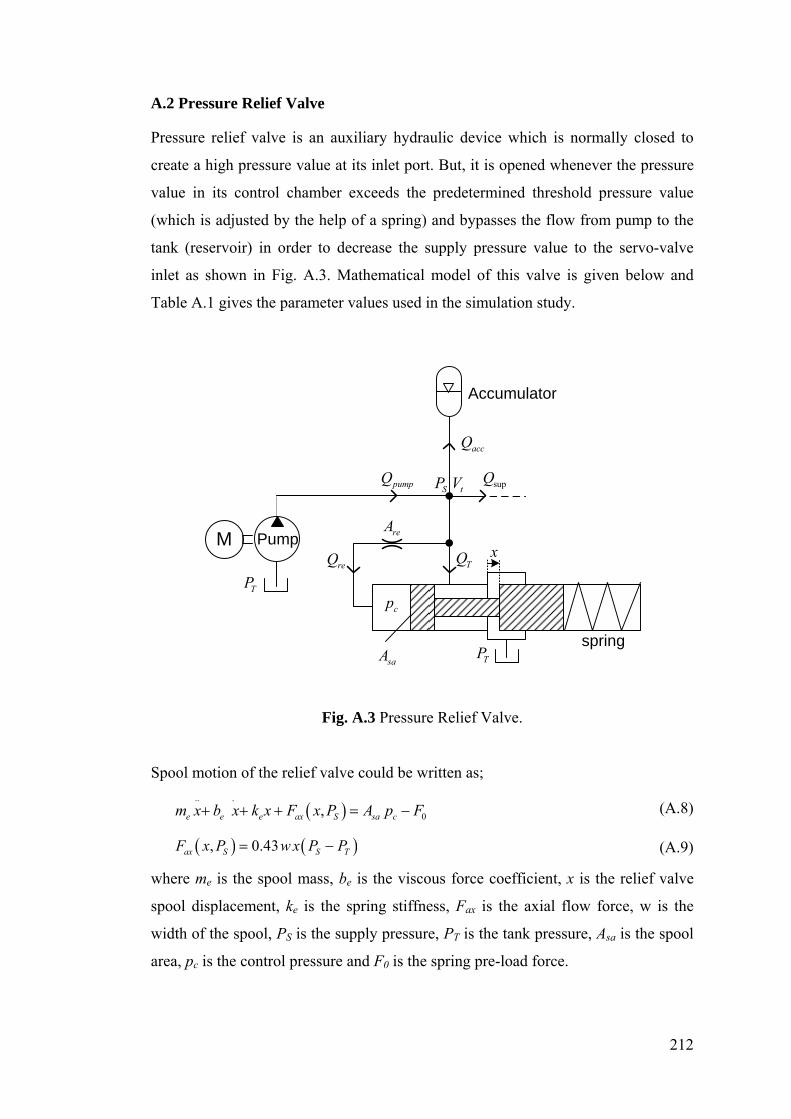
212

A.2 Pressure Relief Valve

Pressure relief valve is an auxiliary hydraulic device which is normally closed to

create a high pressure value at its inlet port. But, it is opened whenever the pressure

value in its control chamber exceeds the predetermined threshold pressure value

(which is adjusted by the help of a spring) and bypasses the flow from pump to the

tank (reservoir) in order to decrease the supply pressure value to the servo-valve

inlet as shown in Fig. A.3. Mathematical model of this valve is given below and

Table A.1 gives the parameter values used in the simulation study.

M

Accumulator

Pump

pumpQ

accQ

supQS tP V

reQ TQ x

TP

TP

cp

saA

reA

spring

Fig. A.3 Pressure Relief Valve.

Spool motion of the relief valve could be written as;

( ).. .

0,e e e ax S sa cm x b x k x F x P A p F+ + + = − (A.8)

( ) ( ), 0.43ax S S TF x P w x P P= − (A.9)

where me is the spool mass, be is the viscous force coefficient, x is the relief valve

spool displacement, ke is the spring stiffness, Fax is the axial flow force, w is the

width of the spool, PS is the supply pressure, PT is the tank pressure, Asa is the spool

area, pc is the control pressure and F0 is the spring pre-load force.

213

Moreover, the control pressure dynamics could be written as below by applying the

flow continuity equations to the control chamber;

( ) ( ) ( ) 2c re sa d re c S c S sa

c co sa

p Q A x A sign p P p P A xV x V A xβ β α

ρ⎡ ⎤

= − = − − −⎢ ⎥+ ⎣ ⎦

(A.10)

where Vc is the volume of the control chamber, Vco is the initial control chamber

volume when the relief valve spool is completely closed, αd is the discharge

coefficient, Qre is the flow through the restrictor and Are is the area of the fixed

restrictor.

Applying the continuity equation to the chamber of the supply pressure leads to

( ).

supS pump re T acct

P Q Q Q Q QVβ

= − − − − (A.11)

( ) 2T d S T S TQ w x sign P P P Pα

ρ= − −

(A.12)

where Vt is the total volume of the chamber where pressure is controlled, Qpump is the

pump flow, Qsup is the supply flow to the servo-valve inlet port, QT is the flow

through the main orifice of the relief valve and Qacc is be the flow to the

accumulator. The parameter values used in the simulation model are given in Table

A.1.

Table A.1 Parameters used in the relief valve model.

Parameter Value Parameter Value me 0.1 kg be 300 Ns/m ke 10000 N/m Asa 1×10-4 m2 F0 2000 N w 0.022 m Vco 1×10-5 m3 αd 0.7 Β 1.4×109 Pa Vt 2×10-3 m3 Are 5×10-8 m2 xmax 0.01 m

214

A.3 Accumulator

Accumulators are primarily used to filter pressure pulsations from the pump and to

provide additional fluid flow in the necessary direction as shown in Fig. A.4.

accP

SPaccQ

gasiV

Fig. A.4 Accumulator dynamics.

The relationship between Qacc and Pacc could be written as follow (Kang et al.,

2008);

( )kk

acc acci gasi gasi accP P V V Q dt= − ∫ (A.13)

( )acc acc leak s accQ K P P−= − (A.14)

where Pacci is the initial pressure, Vgasi is the initial volume of gas, k is the polytropic

exponent of gas and Kacc-leak is the leakage coefficient of the accumulator. The

parameter values used in the simulation study are given in Table A.2.

Table A.2 Parameters used in the accumulator model.

Parameter Value Parameter Value Pacci 2×107 Pa Vgasi 150 ml

k 1.4 Kacc-leak 2×10-10 m3/(Pa⋅s)

A.4 Pump and Motor

In this section, mathematical models of the pump and motor are derived. First, a

gear-box headed DC motor is utilized as the motor of the pump device and then, a

fixed displacement pump is used for flow supply to the hydraulic circuit from the

215

pump exit. It is assumed that a motor having a maximum speed of 12000 rev/min is

used in the simulation study. Moreover, the nominal voltage and power of the motor

are assumed 240 V and 10 kW, respectively. The mathematical equations of the DC

motor and the pump flow (Qpump) are given as below;

diU E L Ridt

= + + (A.15)

c gE K K ω= (A.16)

e t gT K K i= (A.17)

e fric LT J k Tω ω= + + (A.18)

L mechT D p η= (A.19)

pump ilp SQ D K Pω= − (A.20)

where U is the nominal voltage, L is the inductance, R is the resistance, E is the back

electromotive force voltage, Kc is the back emf constant, Kg is the gearbox ratio, Te is

the electromagnetism torque, Kt is the torque constant, J is the total inertia (motor

plus pump system), kfric is the viscous coefficient, ω is the rotational speed of gear-

box output, TL is the load torque, D is the pump displacement, p is the pressure

differential across the pump (if one assumes that tank pressure PT is exactly zero

then p equals to PS) and ηmech is the pump mechanical efficiency. The parameter

values used in the simulation study are given in Table A.3.

Table A.3 Parameters used in the motor and pump model.

Parameter Value Par. Value U 240 V L 2.5×10-3 H R 1 ohm Kc 0.2 V/(rad/s) Kt 0.2 Nm/A Kg 7:1 J 1.2×10-3 kg⋅m2 kfric 4×10-4 N⋅m/(rad/s) D 16 cm3/rev ηmech 0.80

Kilp 1×10-13 m3/(s⋅Pa)

A.5 Pipelines

Pipelines are used to connect the hydraulic elements to each other. Pipeline

dynamics can be neglected assuming the pipe lengths are small. In that case, their

216

volume should be added to the corresponding chamber volumes while solving the

related pressure dynamics there. In the simulation study, only the pipeline dynamics

between the pump and the supply port of the servo-valve is taken into consideration

while assuming the other pipeline lengths are small.

Taking the supply line (going from the pump to the servo-valve inlet) as an example,

p1 and q1 will indicate the pump side pressure and the flow rate at the head of the

pipeline and p2 and q2 will indicate the supply pressure value and supply flow rate at

the inlet of the servo-valve as could be seen from Fig. A.5. The pipeline effects

could be modeled by a four-pole equation (Ayalew and Kulakowski, 2005).

2 2,p q1 1,p q

Fig. A.5 A fluid transmission line.

The four-pole equations in the Laplace domain could be arranged to give the p2(s)

and q1(s) as outputs while the inputs are p1(s) and q2(s) as shown below:

( )( )

( )( ) ( )

( )( )

( ) ( ) ( )

( )( )

2 1

1 2

1cosh cosh

1cosh cosh

c

c

Z s sinh ss sp s p s

q s q ssinh sZ s s s

Γ⎡ ⎤−⎢ ⎥Γ Γ⎡ ⎤ ⎡ ⎤⎢ ⎥=⎢ ⎥ ⎢ ⎥⎢ ⎥Γ⎣ ⎦ ⎣ ⎦⎢ ⎥

Γ Γ⎢ ⎥⎣ ⎦

(A.21)

The propagation operator Γ(s) and the line characteristic impedance Zc(s) are

defined by

( )2

22

324nsds D

v sdα χυαΓ = +

(A.22)

( ) 20 2

32cZ s Z

sdα χυα= +

(A.23)

where α is the natural frequency modification factor and χ is the damping

modification factor, which could be determined from Yang and Tobler (1991).

217

Moreover, υ is the kinematic viscosity. Dn is the dissipation number and Z0 is the

line impedance as given below

2

4n

lDc dυ

= (A.24)

0 2

4 cZdρ

π=

(A.25)

c βρ

= (A.26)

where l and d is the length and diameter of the pipeline, respectively. Moreover, c is

the speed of sound which is expressed in terms of bulk modulus and density of the

hydraulic oil.

Table A.4 shows the value of the parameters used in the pipeline model and a least-

squares curve fit algorithm (Wongputorn et al., 2005) named ‘invfreqs’ in the

MATLAB Signal Processing Toolbox is used to approximate the three casual

functions as below

( )

5 6 4 7 3 14 2

15 21

6 5 8 4 9 3 15 2

16 21

0.358 1.073 10 4.557 10 1.532 101 4.11 10 9.078 10

cosh 102.3 1.052 10 6.964 10 2.732 108.823 10 9.078 10

s s s ss

s s s s s ss

+ × + × − ×

− × + ×=

Γ + + × + × + ×

+ × + ×

(A.27)

( ) ( )( )

14 7 7 6 21 5 24 4

27 3 30 2 31 33

8 7 7 6 11 5 14 4

17 3 20 2 22

2.091 10 5.144 10 3.764 10 7.134 104.673 10 1.17 10 9.951 10 1.732 10

cosh 3675 8.32 10 1.75 10 4.012 105.856 10 3.44 10 7.548 10 4.7

c

s s s sZ s sinh s s s s

s s s s s ss s s

× + × + × + ×

Γ + × + × + × + ×=

Γ + + × + × + ×

+ × + × + × + 2475 10×

(A.28)

( )( ) ( )

7 7 6 5 4 4

7 3 9 2 11 5

8 7 7 6 11 5 14 4

17 3 20 2 23 24

8.758 10 0.0024 16.08 3.621 102.573 10 6.225 10 4.121 10 9.943 10

cosh 2954 7.387 10 1.925 10 4.012 106.773 10 4.615 10 1.11 10 7.345 10

c

s s s ssinh s s s s

Z s s s s s s ss s s

× + + + ×

Γ + × + × + × − ×=

Γ + + × + × + ×

+ × + × + × + ×

(A.29)

218

Table A.4 Parameters used in the pipeline model.

Parameter Value Parameter Value d 0.005 m l 1 m v 100 mm2/s ρ 890 kg/m3 β 1.4×109 Pa α 1 χ 1

A.6 Hydraulic Cylinder Dynamic and Friction Model

Here, the model of the hydraulic cylinder is developed by taking the effects of

position dependent actuator chamber volumes and friction forces. The internal and

external leakages are also taken into consideration as shown in Fig. A.6.

Hydraulic cylinder

x

Load Mass M

B

K

Friction

AQ QB

P A PB

Piston displacement

,A AP V ,B BP V

int_ leakQ_ext leakQ

_ext leakQpA

Fig. A.6 Hydraulic cylinder.

Applying the continuity equations to each cylinder chamber will give the chamber

pressure dynamics as below.

0int_ _

A p AA leak ext leak p

V A x dPQ Q Q A xdtβ

+⎛ ⎞− − − = ⎜ ⎟

⎝ ⎠ (A.30)

int_ _B p B

B leak ext leak p

V A x dPQ Q Q A xdtβ

−⎛ ⎞− + − + = ⎜ ⎟

⎝ ⎠ (A.31)

Moreover, the nonlinear equation describing the relationship among the chamber

pressures and the actuator position (x) can be written as

( )A B p fricP P A M x B x Kx F− = + + + (A.32)

where Μ is the mass of the piston/load; Β is the the effective viscous damping; K is

the stiffness of the equivalent spring, Αp is the piston annulus area and β refers to the

bulk modulus of the hydraulic fluid. PA and PB denote the hydraulic pressures in

219

each of the actuator chambers. Note that the volumes of hydraulic oil on each side of

the piston are given by variables VA=Apx+VA0 and VB=-Apx+VB0 where VA0 and VB0

are the initial chamber volumes. The internal and external leakages (Qint_leak and

Qext_leak) can be calculated as Cint (PA-PB) and Cext PA (or Cext PB ), respectively, where

Cint and Cext will be the leakage coefficients. On the other hand, friction process in

(A.33) can be characterized by the LuGre model as its mathematical model is given

in (5.7) and (5.8). The parameter values used in the simulation study are also given

in Table 5.1.

220

APPENDIX B

MATLAB FILES

The below M-Files are used to create and to train network objects which are

presented in Chapter 5. In Appendix B.1, Network_Qa (in Fig. 5.4) is devised. In a

similar way, Network_Qb could also be created. Next, Appendix B.2 represents the

M-File for the creation of the divider network as illustrated in Fig. 5.5. Furthermore,

the construction of the SRNN from its modules (Network_Qa, Network_Qb and

divider network) is realized by the M-File given in Appendix B.3.

B.1 M-File for the Network_Qa

u = linspace(-1,1,99)'; p = linspace(0,1,99)'; q = zeros(99,99); output=zeros(1,9801); input=zeros(2,9801); k=1; for i = 1:99 for j = 1:99 if(u(j)>0) q(i,j) = u(j)*sqrt(1-p(i)); else q(i,j) = u(j)*sqrt(p(i)); end output(k)=q(i,j); input(1,k) = u(j); input(2,k) = p(i); k=k+1; end end net = network; net.numInputs = 2; net.numLayers = 3; net.biasConnect = [1; 1; 1]; net.inputConnect(1,1) = 1; net.inputConnect(1,2) = 1; net.layerConnect = [0 0 0;1 0 0;0 1 0]; net.outputConnect = [0 0 1]; net.inputs{1}.size = 1;

221

net.inputs{1}.range = [-1 1]; net.inputs{2}.size = 1; net.inputs{2}.range = [0 1]; net.layers{1}.size = 10; net.layers{1}.transferFcn = 'tansig'; net.layers{1}.initFcn = 'initnw'; net.layers{2}.size = 10; net.layers{2}.transferFcn = 'tansig'; net.layers{2}.initFcn = 'initnw'; net.layers{3}.initFcn = 'initnw'; net.initFcn = 'initlay'; net.performFcn = 'mse'; net.trainFcn = 'trainlm'; net = init(net); net.trainParam.goal = 1e-10; net.trainParam.epochs=2500; net = train(net,input,output); Network_Qa=net;

B.2 M-File for the divider network

u = linspace(-1,1,100)'; p = linspace(-0.9,0.9,100)'; q = zeros(100,100); output=zeros(1,10000); input=zeros(2,10000); k=1; for i = 1:100 for j = 1:100 q(i,j) = u(j)/(p(i)+1); output(k)=q(i,j); input(1,k) = u(j); input(2,k) = p(i); k=k+1; end end net = network; net.numInputs = 2; net.numLayers = 2; net.biasConnect = [1; 1]; net.inputConnect(1,1) = 1; net.inputConnect(1,2) = 1; net.layerConnect = [0 0;1 0]; net.outputConnect = [0 1]; net.inputs{1}.size = 1; net.inputs{1}.range = [-1 1]; net.inputs{2}.size = 1; net.inputs{2}.range = [-0.9 0.9]; net.layers{1}.size = 20; net.layers{1}.transferFcn = 'tansig'; net.layers{1}.initFcn = 'initnw' net.layers{2}.initFcn = 'initnw'; net.initFcn = 'initlay'; net.performFcn = 'mse';

222

net.trainFcn = 'trainlm'; net = init(net); net.trainParam.goal = 1e-20; net.trainParam.epochs=1000; net = train(net,input,output); divider=net;

B.3 M-File for the SRNN net = network; net.numInputs = 4; net.numLayers = 10; net.biasConnect = [1; 1; 1; 1; 1; 1; 1; 0; 1; 0]; net.inputConnect(1,1) = 1; net.inputConnect(4,1) = 1; net.inputConnect(7,2) = 1; net.inputConnect(9,4) = 1; net.inputConnect(7,3) = 1; net.inputConnect(9,3) = 1; net.layerConnect = [0 0 0 0 0 0 0 1 0 0; 1 0 0 0 0 0 0 0 0 0; 0 1 0 0 0 0 0 0 0 0; 0 0 0 0 0 0 0 0 0 1; 0 0 0 1 0 0 0 0 0 0; 0 0 0 0 1 0 0 0 0 0; 0 0 1 0 0 0 0 0 0 0; 0 0 0 0 0 0 1 1 0 0; 0 0 0 0 0 1 0 0 0 0; 0 0 0 0 0 0 0 0 1 1]; net.outputConnect = [0 0 0 0 0 0 0 1 0 1]; net.layerWeights{1,8}.delays = [1]; net.layerWeights{4,10}.delays = [1]; net.layerWeights{8,8}.delays = [1]; net.layerWeights{10,10}.delays = [1]; net.layers{1}.size = 10; net.layers{1}.transferFcn = 'tansig'; net.layers{1}.initFcn = 'initnw'; net.layers{2}.size = 10; net.layers{2}.transferFcn = 'tansig'; net.layers{2}.initFcn = 'initnw'; net.layers{3}.initFcn = 'initnw'; net.layers{7}.size = 20; net.layers{7}.transferFcn = 'tansig'; net.layers{7}.initFcn = 'initnw'; net.layers{8}.initFcn = 'initnw'; net.layers{4}.size = 10; net.layers{4}.transferFcn = 'tansig'; net.layers{4}.initFcn = 'initnw'; net.layers{5}.size = 10; net.layers{5}.transferFcn = 'tansig'; net.layers{5}.initFcn = 'initnw'; net.layers{6}.initFcn = 'initnw'; net.layers{9}.size = 20; net.layers{9}.transferFcn = 'tansig'; net.layers{9}.initFcn = 'initnw'; net.layers{10}.initFcn = 'initnw'; net.performFcn = 'mse'; net.trainFcn = 'trainlm';

223

net.initFcn = 'initlay'; net = init(net); net.IW{1,1}=Network_Qa.IW{1,1}; net.IW{4,1}=Network_Qb.IW{1,1}; net.LW{1,8}=Network_Qa.IW{1,2}; net.LW{4,10}=Network_Qb.IW{1,2}; net.LW{2,1}=Network_Qa.LW{2,1}; net.LW{5,4}=Network_Qb.LW{2,1}; net.LW{3,2}=Network_Qa.LW{3,2}*Kv*sqrt(Ps)*Uv_max/q_max; net.LW{6,5}=Network_Qb.LW{3,2}*Kv*sqrt(Ps)*Uv_max/q_max; net.IW{7,2}=divider.IW{1,2}; net.IW{9,4}=divider.IW{1,2}; net.IW{7,3}=-divider.IW{1,1}; net.IW{9,3}=divider.IW{1,1}; net.LW{7,3}=divider.IW{1,1}; net.LW{9,6}=-divider.IW{1,1}; net.LW{8,7}=divider.LW{2,1}*q_max*Bulk/v_A*Ts/Ps; net.LW{10,9}=divider.LW{2,1}*q_max*Bulk/v_B*Ts/Ps; net.LW{8,8}=1; net.LW{10,10}=1; net.b{1,1}=Network_Qa.b{1,1}; net.b{2,1}=Network_Qa.b{2,1}; net.b{3,1}=Network_Qa.b{3,1}*Kv*sqrt(Ps)*Uv_max/q_max; net.b{4,1}=Network_Qb.b{1,1}; net.b{5,1}=Network_Qb.b{2,1}; net.b{6,1}=Network_Qb.b{3,1}*Kv*sqrt(Ps)*Uv_max/q_max; net.b{7,1}=divider.b{1,1}; net.b{9,1}=divider.b{1,1}; SRNN=net; View(SRNN)

224

CIRRICULUM VITAE

PERSONEL INFORMATION:

Name : Ergin Kılıç

Place of Birth : Tokat

Adress : Middle East Technical University,

Mechanical Engineering Department,

A-102, 06800, Ankara.

GSM : [+90] (505) 418 07 15

e-mail : [email protected]

[email protected]

Nationality : Turkish

EDUCATION:

2007 –

: Ph.D. Programme at METU

CPGA: 3.75/4 (Graduate Courses Performance Award)

2004 – 2007

: M.Sc. Programme at METU

CPGA: 3.6/4

1999 – 2003

: B.Sc. Programme at Gazi University

CPGA: 3.38/4 (Honor Student)

1992 – 1999

: High School Degree from Çankaya Atatürk Anadolu Lisesi,

Ankara

LANGUAGES:

English : Intermediate (KPDS=72)

WORK EXPERIENCE:

2005 – : Teaching Assistant at ME Department, METU, Ankara.

225

2008 - 2010 : Researcher in a TUBITAK project named as “Development of

Personal Computer based Universal Motion Control Systems”

(project no: 108E048).

2003 – 2004 : Sales Engineer at Altar Teknoloji, Kavaklıdere, Ankara .

COMPUTER SKILLS:

Autodesk\ AutoCAD : Medium

Autodesk\ Inventor : Professional

SolidWorks : Medium

KeyCreator : Medium

EdgeCAM : Medium

MATLAB : Professional

JAVA : Beginner

C# : Beginner

Verilog : Medium

VHDL : Beginner

INTERESTS AND HOBBIES:

Fitness, Traveling, Electronics

PUBLICATIONS:

Kilic, E., Dolen, M., Koku, A.B., Caliskan, H. and Balkan, T. Accurate pressure

prediction of a servo-valve controlled hydraulic system. Mechatronics, doi:

10.1016/j.mechatronics.2012.08.001

Kilic, E., Dogruer, C.U., Dolen, M. and Koku, A.B. 2012. Position estimation for

timing belt drives of precision machinery using structured neural networks.

Mechanical Systems and Signal Processing, 29, 343-361.

Kilic, E., Dolen, M. and Koku, A.B. 2010. Analysis and estimation of motion

transmission errors of a timing belt drive. Turkish Journal of Electrical Engineering

and Computer Sciences, 18(5), 883-897.

226

Dogruer, C.U., Kilic, E., Dolen, M., and Koku, A.B. 2007. Nonlinear position

estimators based on artificial neural networks for low costs manufacturing systems.

Journal of Automation, Mobile Robotics and Intelligent Systems, 1(2), 40-44.

Kilic, E., Dolen, M., Koku, A.B. and Dogruer, C.U. 2007. Novel position estimators

for timing belt drives. Journal of Automation, Mobile Robotics and Intelligent

Systems, 1(2), 55-61.

Kanburoglu, F.A., Kilic, E., Dolen, M. and Koku, A.B. 2007. A test setup for

evaluating long-term measurement characteristics of optical mouse sensors. Journal

of Automation, Mobile Robotics and Intelligent Systems, 1(2), 71-75.

INTERNATIONAL CONFERENCES:

Kilic, E., Dolen, M. and Koku, A.B. 2011. Experimental Evaluation of Cable-Drum

Systems as Linear Motion Sensors. In Proceedings of IEEE International

Conference on Mechatronics, Turkey, pp. 666-671.

Kilic, E., Dolen, M. and Koku, A.B. 2011. Long-term prediction of hydraulic system

dynamics via structured recurrent neural networks. In Proceedings of IEEE

International Conference on Mechatronics, Turkey, pp. 330-335.

Kilic, E., Baser, O., Dolen, M. and Konukseven, E.I. 2010. An enhanced adaptive

windowing technique for velocity and acceleration estimation using incremental

position encoders. In Proceedings of the International Conference on Signals and

Electronic Systems, Gliwice, Poland, pp. 61-64.

Baser, O., Kilic, E., Konukseven, E.I. and Dolen, M. 2010. A hybrid method to

estimate velocity and acceleration using low-resolution optical incremental

encoders. In Proceedings of the International Conference on Signals and Electronic

Systems, Gliwice, Poland, pp. 57-60.

227

NATIONAL CONFERENCES:

Ergin Kılıç, Hakan Çalışkan, Melik Dölen, A. Buğra Koku, and Tuna Balkan. 2011.

Yapay sinir ağ modellerinin valf denetimli hidrolik bir sistemin uzun süreli basınç

tahmininde kullanılması. 6th National Hydarulic Pneumatic Congress and Exhibition

(HPKON 2011), 12-15 October, Izmir, pp. 211- 225.

Furkan A. Kanburoğlu, Ergin Kılıç, Melik Dölen and A. Buğra Koku. 2009.

Bilgisayar denetimli takım tezgahları için dağıtık bir hareket denetim sistemi.

National Conference on Automatic Control (TOK’09), 13-16 October, Istanbul, pp.

483-489.

Ergin Kılıç, Melik Dölen ve A. Buğra Koku. 2008. Dişli kayış mekanizmalarında

iletim hatalarının incelenmesi. National Conference on Automatic Control

(TOK’08), 13-15 November, Istanbul, pp. 200-205.

structured neural networks for modeling and identification of nonlinear...

Documents