Investment Product Research

A DESCRIPTION OF CALCULATIONS

September 2017

INTRODUCTION

Investment Product Research offers clear and fair quantitative research on

structured products. Our primary aim is to give advisers and investors an

indication of the risk and return that a product offers, relative to other

products.

Our analysis can therefore be used to RANK products, but does

NOT provide reliable information on FUTURE returns or

probabilities of events.

Our analysis allows products to be filtered to identify a short list of

products that may be suitable, and then ranked using a number of

different measures to help identify the product that best meets the

investor’s requirements.

2

CONTENTS

PAGE

1. METHODOLOGY 3

2. PRODUCT ANALYSIS 3

3. OUTPUT 7

4. PRODUCT LISTING ENTRY 8

5. CALCULATIONS 10

6. PRIIPS 19

7. TABLES AND CHARTS 21

3

1. Methodology

We measure risk and return using historical data only:

- We use publicly available data that is available through external sources such as

Bloomberg

- Our analysis is fully transparent, objective and verifiable

- There is no need for specialist derivatives knowledge

- We are not required to make any assumptions, estimates or judgments

We use straightforward methodologies, applied consistently across all products

- We offer clear analysis of the risks and returns a product offers

We calculate the product’s “volatility”

We map this volatility to a number of risk scores

We calculate a range of “expected” returns that a product offers

- Our analysis makes product comparison straightforward;

compare products to benchmark equity / bond portfolios

compare products from different issuers

compare products with exposure to different underlying markets

- There is no need for specialist statistical or mathematical knowledge to understand

the analysis

- Our analysis metrics are consistent with the risk information offered by funds in their

Key Investor Information Documents (KIIDs)

- Our analysis metrics are consistent with mainstream financial planning tools and

processes

2. Product Analysis

Product analysis is all interactively available online and can be accessed digitally using our

APIs, or pdf document generator. The analysis is updated weekly throughout product life,

reflecting the current product price and the latest levels of the underlying assets and other

market data - please refer to the “Dealing with products post-strike” section for further

details.

MULTIPLE SCENARIOS

We test products under different scenarios

4

- Historic Back-test; an analysis of the risks and returns offered by a product that uses

the actual past performance of the underlying assets

- Future Stress-test; the same analysis but on multiple re-sampled paths of the

historical returns of the underlying data

- Credit Adjusted Future Stress-test; an adjusted Future Stress-test where the risks

and returns are adjusted to reflect the possibility of the issuer defaulting

- UKSPA analyses (Bear, Neutral and Bull); we do not discuss this further as details can

be found on the UKSPA site

- PRIIPs; details are given in a later section

I. Historic Back-test methodology

We use daily closing levels of a product’s underlying(s) as far back as possible to analyse the returns that a product would have offered had it been available in the past.

To illustrate, we describe how on 15th

May 2015 we would have back-tested a 6 year autocall with annual kick-outs from Year 2 and a 50% American soft protection barrier, with an underlying whose first data point is 31

st

December 1986:

- the first 6-year cycle we look at is therefore 31st

December 1986 to 31st

December 1992

- the second is 2nd January 1987 to 2nd January 1993 and so on, each cycle starting and ending on a trading day

- the last cycle is 15th

May 2009 to 15th

May 2015 as this is the last complete 6 year term

- There are 5770 such cycles

For each cycle, we first check if the product would have kicked out in Year 2. If so, it is recorded as a Year 2 early maturity and no further analysis is needed for that cycle. If not, we then check if it would have kicked out in Year 3 and so on through to Year 6.

We cannot select cycles starting later than 15th

May 2009 as the six year term would not have been completed. This is the case even when we know that on some of those occasions the product would have matured early. To include such cycles would be to “cherry pick” as only those that had matured early would be included; cycles where the product would not yet have matured and which could end in a capital loss would be left out and therefore would present a misleading result.

We can then analyse the outcomes and record how many of the 5770 cycles would have resulted in a Year 2 kick out, Year 3 kick out, Year 4 kick out, Year 5 kick out, Year 6 growth payment, a maturity payment equal to the capital invested or a capital loss at maturity.

The results can be presented as a percentage of the population of 5770 cycles. For example, 4720 Year 2 kick outs is 81.8% of the 5770 possible start dates; similarly 58 occasions where a capital loss occurred is 1% of the possible start dates.

The same principles can be applied to other structures. For example, with the same basic product shape linked to the several indices, we would start from the earliest common data date for all indices. Although the time span is the same, there will be fewer observations, as the back-test can only use a start date when both indices are quoted.

Our research is not restricted to fixed start dates however. It will facilitate a time period of the user’s choosing. For example, if an analyst were to assume that only the last 10 years of data were relevant, on our site they could set the start date to reflect only this period of data. The number of cycles would then be reduced to only the last 10 years.

5

II. Future Stress-Test

Having only 1 sample of history constrains risk analysis:

- For example, some products would have had no, or a very small number of cycles that would have led to capital losses, despite the fact that the product structure has clear downside exposure and the fact that the investor is able to earn a significant additional potential return from assuming this risk. Placing such products in a low risk category may seem inappropriate

- Other products might have a structure that captures a current pricing opportunity to meet investor needs but which back-testing might show as having a poor historical record. Placing such products in a high risk category may seem equally inappropriate

Put another way; past performance is not a reliable indicator of future performance and should not be used to assess future returns or risks. Nobel prize-winner Paul Samuelson (and many other leading economists) highlighted the fallacy in simply taking realised market returns (as the Historic Back-test does) as statistically significant proof of performance – statistically speaking, history is just one sample from a much larger distribution of possibilities.

Resampling the available data is a well-established1 way of representing the true underlying distribution of

possibilities, enabling a statistically more correct assessment of risk. Resampling is a process that is simple, straightforward and robust.

As outlined in the Historic Back-test section above, there are 5770 dates on which a six year product might have started and reached the end of a six year term. This is just one dataset. Resampling allows for the creation of multiple datasets which explore more fully the range of possible movements in the underlyings.

In order to determine the possible future movement in the underlying, we look at what the range of daily movements has been in the past for the index and use these to create new index series. On most days the Index does not move by large amounts – it may go up a little, go down a little or remain flat. On other days, the daily change might be more exaggerated and on comparatively fewer days there will be extreme movements.

The first step is to compile a new dataset from the information that we have. We can set the new initial index price base level at 100.

A particular date is selected at random from all of the possible start dates in the data history that we are using

2, for example date 3214. The close of business level on date 3214 is recorded and compared to the level

at close of business on day 3215. This gives us the movement for the Index on that day. Let’s say that it was 1% up.

The Index level at the end of the first “day” of our new index is therefore 101 (i.e.100 increased by 1% or 100 x 1.01). This is repeated until we have enough simulated data for the product’s remaining time to maturity.

As the selection is random, any one day return can be selected again, and so could be used more than once as part of the resampling process. Some daily returns may not get selected at all. We then carry out back-testing on the newly constructed dataset in exactly the same way as we did for the single historical back-test of the actual index performance.

We repeat this process multiple times until the results we get are stable3, typically in the region of 100,000

iterations. At this point we can be confident that the values that we are able to derive from the resampling process will represent the likely future range of returns of the underlying assets, that this range will remain

1 For example, resampling relies on the well-proven (weak) efficient markets hypothesis, as

do the entire fund management and derivatives industries

2 1992-12-31 is our standard start date for the data window we resample from 3 i.e. further iterations would not bring about statistically meaningful changes in the results

6

constant, and so the results that we derive from the stress-test will not vary materially from one test to another.

This resampling process means the much larger number of potential histories tested gives a more detailed view of the distribution of potential product outcomes and therefore enables more robust estimates of performance statistics.

III. Credit Adjusted Future Stress-Test

We also calculate a set of risk and return numbers that reflect any additional risk that an investor is exposed to from possible issuer default.

For each single cycle we assume that the final value is either

- The value that we have calculated using the re-sampled data

- 40% of the value calculated using the re-sampled data

The process is random, but the proportion of cycle results that are adjusted down will be based on the chance of default that we calculate. This process that we use implies that the issuer is as likely to default if the underlying assets have increased in value as when the underlying assets have fallen in value.

The chance of default is calculated using the issuer’s CDS levels, and an assumed 40% recovery rate. The 40% recovery rate assumes that in the event of issuer default investors will receive 40% of the value of the product when it matures. 40% is a market standard recovery rate that is typically used to calculate these figures; expected returns are not very sensitive to the choice of assumed recovery rate.

The credit adjustment will reduce the expected gains and reduce the chance of a gain since if there is a default, some of the instances where an investor would have made a profit will now be loss making. The credit adjustment will both increase the chance of a loss, and increase the expected loss. As a result the credit adjusted risk-return ratio and Win Lose ratios will both be lower.

DEALING WITH PRODUCTS POST-STRIKE The analysis described above is applied equally to post strike products. It is useful nevertheless to describe how products present themselves to the analysis once they have struck. Basically, post-strike, a product now has fixed strikes, with a time to maturity that gradually decreases. For example a product with a kickout barrier on the first anniversary of 100% will have a barrier of 900.00 if this is the closing price on the strike date. If we evaluate this product 9 months later, when the underlying has a closing price of 1000.00:

This barrier level is now 90% of the prevailing spot level

So in our simulations we set this barrier level to 90% of the simulated starting level of the underlying

And we set the barrier observation date to be 3m in the future, since 9m have already elapsed

In this way we analyse a product as it really is on the evaluation date. Similar calculations are used to reflect product features that are part-way through, for example, an averaging period, or a lookback period etc.

USER-SPECIFIED PARAMETERS Rather than use historical or resampled data, users can elect to use, for any particular product, their own parameters. Currently we provide a standard diffusion process (multivariate geometric Brownian motion “GBM”) and users can enter their own drift rate curves, volatility surfaces and correlation matrices. All of these are accessible from our Admin page.

As a result, each user has their own private set of global parameters: in other words there is, for example, one SX5E volatility surface which will apply to all that user’s user-specified-parameters products.

7

Since user-specified parameters make market-wide product comparison difficult, any product using user parameters will not be visible on the IPR public Listing; it will still of course be visible on the Listing for that logged-in user.

3. Output

PRODUCT LIST

The Product listing gives searchable and sortable details of the entire product database: users can screen and filter products, change column headings, and:

- choose which analyses to display (eg PRIIPs, UKSPA)

- choose which analysis metrics to use as sortable column headings

- view detailed analysis of risk and return

- view detailed probability of early maturity and barrier breach

- generate full PDF reports

SCREENING PRODUCTS

Each investor will have different requirements, their attitude to risk will be different and they will have a different capacity for loss. The variables that we publish will allow unsuitable products to be eliminated from consideration.

For many investors product risk is one of the most important suitability factors. We calculate a number of ways to look at risk: volatility (and its mapping to a range of risk scores), estimated “worst case” returns and payoffs, the chance of loss, and so on.

Investors are of course concerned about the returns that they should expect; they may want to eliminate products that do not offer enough potential return.

Both the risk and return scores can be used with, and without, a credit adjustment. Our credit adjustment process uses the issuer’s bond spreads and market CDS rates. These may be rates the investor agrees with, or which they feel does not reflect the creditworthiness of the issuer. We also give issuer credit rating, which is another possible screen.

RANKING PRODUCTS

Having identified if a product meets an investor’s minimum requirements there are a number of ways they can be ranked: we offer a comprehensive set of risk/return metrics as sortable analysis columns; for example, investors can rank products on the overall expected return, or on the positive return that they may receive; other investors could alternatively rank products based on a chosen risk score or volatility.

Our online analysis has these sections

- Efficient Frontier

All screened products are plotted on a scatter chart whose axes can be chosen by the user; we also plot a guide line between a cash asset and an equity index

- Product-by-product Tables

Product terms and issuer details

8

Summary Statistics

Payoff analyses

- Charts

Historic backtest charts

Future stress-test chart

Performance chart, where historic product prices are available

4. Product Listing entry Each product has a row in the Listing, which can be clicked to give details:

Static data

Summary metrics

The columns of these tables can be chosen by the user:

9

Scenario metrics

These tables are updated after the strike date to show barrier levels, trigger levels and other reference data as specific levels and also as a % of the current underlying level(s).

Coupon metrics

-

5. Calculations

Our Expected Return reflects the geometric average of the returns realised in repeated simulations of

investment in the product. We use the geometric average because it produces a CAGR figure, which

can be compared across products and asset classes with different time horizons. Note that all our

other return numbers, such as conditional gain, are arithmetic averages (of the returns realised in

repeated simulations of investment in the product) and therefore should not be interpreted as CAGR

figures.

Return calculations

Expected Return (%pa)

The expected return is the annualised expected return obtained from all simulated product episodes. For example, an expected return of 41.85% after 6 years is the equivalent of 6% per annum (1.06^6 – 1 = 41.85%). But for kick-outs, the payoff P can occur at different times T and with an associated probability. The return is therefore calculated as an annualised return

exp( ∑ 𝒍𝒏(𝑷𝒊)𝑵𝒊=𝟏 / ∑ 𝑻𝒊

𝑵𝒊=𝟏 ) – 1

Where Pi is the payoff4 at time Ti of the i-th product instance

The expected return reflects all of the outcomes, good and bad, that the product has delivered under each scenario. As such it is a good reflection of the return that the product will offer.

Arithmetic Return (%pa)

The arithmetic return is the annualised return based on the expected payoff and duration:

pj Pj) ^ (1/pj Tj) - 1

Where pj is the probability of scenario j which occurs at time Tj and whose arithmetic average payoff is Pj

It reflects the average payoff, annualized by the average time to maturity, and is typically somewhat higher than the Expected Return above.

CouponReturn

This is the arithmetic average of the simulated annualized returns, where each such return references ONLY

the sum of (a) the value of all product coupons (forward-valued to the payout date if necessary) and (b) a FULL

repayment of the product notional – so the coupon return will include any “pull-to-par” return.

IRR

All simulation cashflows are accumulated and the IRR is their annualized internal rate of return; ie the return which gives a zero present value of all cashflows.

Excess return (%pa)

4 eg 1.15 representing a 15% gain

11

Arithmetic return minus a "benchmark" return of:

(6y GBP swaps) + 5yCDS/2 + (Product volatility/TUKXG volatility)/(TUKXG ArithmeticReturn - 6y GBP swaps)

The “benchmark” return reflects a fair hurdle for product volatility and issuer funding/credit.

Expected Payoff

pt Pt

For example, suppose a product pays:

- 40% growth at maturity if the Index is at or above its Initial Level,

- Capital return only if Index is below its Opening level but no breach of the protection barrier, and

- Capital reduced if the protection barrier is breached

Let’s say our results show 75% of occasions resulted in a 40% payment, 20% resulted in capital return only (0% growth) and 5% ended in a loss averaging 43%, the expected pay off would be 75%*40% + 20%*0%+5%*-43% = 27.85%.

The same calculations can be used for kick out plans but using the individual autocall coupons payable in any one year multiplied by the proportional incidence of autocalls in that year

Win Lose Ratio

This is the ratio of the total annualised returns of (1) all product instances with positive returns; (2) all product instances with negative returns

5. It measures the relative amounts of “win” and “lose” returns.

Rgain / Rloss

Where:

Rgain is the return for a product instance that was a gain

Rloss is the return for a product instance that was a loss

The Win/Lose ratio is a ratio that we have developed to help rank products. A high Win Lose ratio means that the product offers a greater number of wins for each unit of loss. It is an alternative to the risk / return ratio and reflects the probability, term and scale of winning and losing outcomes. We developed this ratio to better reflect the variable term that is a common feature of structured products, but it can just as easily be used to evaluate equities, bonds and other assets.

Features of WinLose:

Easy to understand and interpret

Easy to estimate

Combines all “moments” of the returns distribution: mean,variance,skew,kurtosis and so on; this contrasts with some statistical measures (eg modified VaR) which use unstable

6 statistics (ie

summaries) of the data; WinLose uses all the data and therefore provides a more comprehensive product ranking than SharpeRatios, VaR,modifiedVaR, etc

5 An alternative description is the ratio: ExpectedConditionalGain/ExpectedConditionalLoss

6 use cubes and fourth powers of the data

12

Produces sensible product Ranking: a product with a higher WinLose is better7

Risk Return Ratio

This is the ratio of expected return to volatility, and shows the expected return for every unit of risk.

The risk return ratio uses our volatility calculation as the measure of risk, and the expected return calculation as the measure of return.

Combo Ratio

This is the ratio of non-credit-adjusted expected return to credit-adjusted volatility, and shows the expected return for every unit of risk including credit risk.

The risk return ratio uses our credit-adjusted volatility calculation as the measure of risk, and the expected return calculation as the measure of return.

Conditional Gain (%pa)

Rgain / gain

For outcomes that result in a gain (defined as an annualized return >= 0), this shows the average size of that gain.

Where:

Ngain is the number of product instances that resulted in a gain

Rgain is the annualised return for a product instance that was a gain

The conditional gain is the average gain for instances where there has been a gain. It is a measure of the potential profit of a product.

Probability of Gain

gain /

Where:

Ngain is the number of product instances that resulted in a gain (where the payoff is equal to or exceeds

the initial investment) compared to the total number of product cycles.

The probability of gain is self-explanatory. It is a calculation of the proportion of the outcomes that have resulted in a return equal to or greater than the current asset prices. For new products offered at 100%, this will mean that this is the proportion of outcomes where the final value is equal to or greater than 100%. Once a product has struck this will reflect the proportion of outcomes where the final value is greater than the current product price.

7 The only assumption is that more is better; there are no risk-preference or utility

assumptions

13

Expected Gain

gain /×Rgain / gain)

Which is equivalent to the Probability of Gain multiplied by the Conditional Gain, annualised.

Multiplying the conditional gain by the probability of a gain generates an expected gain, or a probability adjusted gain. This reflects both the chance of a gain, and the scale of the gain that is expected.

Expected Gain Payoff

Same as ExpectedPayoff, but only for those Pt >= initial investment.

Conditional Strict Gain (%pa)

Same as ConditionalGain, but only for those Rgain > 0 (ie strictly greater than zero).

Probability of Strict Gain

Same as ProbabilityOfGain, but only for those product instances whose payoff is strictly greater than the initial investment.

Expected Strict Gain Payoff

Same as ExpectedPayoff, but only for those Pt > initial investment.

Probability of No Gain or Loss

zero /

Where Nzero is the number of product instances whose payoff is exactly equal to the initial investment.

Risk calculations

Volatility of Returns

Since risk should measure downside, we believe volatility should be measured from the left tail of a product’s distribution. We use a version of the CESR methodology that was proposed to calculate the volatility of a structured product so that they can be ranked using the same volatility based Synthetic Risk and Return Indicator (SRRI) as funds. We find a normal distribution with the same arithmetic average return whose left tail (or Expected Tail Return) matches that of the product’s distribution of returns:

- Start with the distribution of annualized returns from the product simulations described above; please note that the following calculations use arithmetic averages

- Compute the arithmetic average annualised return for all product instances below the 90th confidence level (the left tail) – call this the product’s Expected Tail Return (see definition above)

14

- Find the standard deviation of a normal distribution of returns (with mean the Expected Return) whose Expected Tail Return below the 90% confidence level is the same as the product’s Expected Tail Return; this quantity is the volatility

Suppose a product has an arithmetic average return of 5%8, ExpectedTailReturn of minus 8%, and duration of

4y. A normal distribution with mean 5% must have a standard deviation 7.4% to produce an ExpectedTailReturn of minus 8%

9. Hence the product’s annualised returns have a volatility of 7.4%. The

product’s payoff volatility is therefore 14.8% since the volatility scales with root time (4=2 in this case). A more detailed example is given as Appendix A.

Calculating volatility this way lets us compare the riskiness of a product’s potentially unusual payoff profile (non-normally distributed) with the riskiness of a fund or other asset with a more normal distribution.

It is important to note that the volatility calculation is not an estimate of the fluctuation of day-to-day returns but instead a reflection of the risk of a product. The calculated volatility for equity based products will reflect the propensity for equity markets to occasionally fall significantly. These so called “fat tails” will increase the calculated volatility of equity based products

The calculated volatility can and will vary once the product has struck, and the terms have been fixed.

Risk Scores

For our standard risk score we have used the risk buckets that are prescribed by CESR. These buckets define a 1 to 7 risk score based on volatility. We also provide a score based on a linear scale from 1 to 10. We use the volatility that we have calculated using the process above. The table below describes the upper and lower volatility bands for each bucket.

8 This is not our ExpectedReturn which is a geometric CAGR-type number as described; typically you can obtain the

arithmetic average return as the probability-weighted average return from our scenarios tables

9 ExpectedTailReturn for the left p% tail of a standard normal distribution is, in Excel terms,

=NORM.S.DIST(NORMSINV(p),FALSE)/p or minus 1.75 for p=0.1; we can in this case equate to the normalized

shortfall of (5 minus -8)/volatility, ExpectedTailReturn so that volatility = 13/1.75 = 7.4

VOLATILITY RANGE RISK

SCORE

0% 0.5% 1

0.5% 2% 2

2% 5% 3

5% 10% 4

10% 15% 5

15% 25% 6

25% 7

VOLATILITY RANGE RISK

SCORE 1to10

0% 2.6% 1

2.6% 5.2% 2

5.2% 7.8% 3

7.8% 10.4% 4

10.4% 13.0% 5

13.0% 15.6% 6

15.6% 18.2% 7

18.2% 20.8% 8

20.8% 23.4% 9

23.4% 26.0% 10

26.0% 11

Where product volatility falls within a range, we interpolate the Risk Score linearly so that 18% volatility, for example, translates to a Risk Score of 6.3.

The risk score for a structured product allows advisers to calibrate the risk of a structured product versus the risk of a fund. Although the method of calculation is different (the volatility of funds is calculated using historic daily returns) the risk score has been designed to be comparable.

VaRxxReturn

The (100-xx) th

percentile annualized return from all product episodes; for example the VaR90Return is the 10th

percentile annualized return, for example, the 100

th-worst annualized return from 1000 episodes.

Expected Tail Return10 (%pa)

∑ 𝑹𝒊𝑵∗𝟎.𝟏𝒊=𝟏 / (N*0.1)

This is the average of the worst 10% annualised returns R. So if there are 100,000 instances we sort them and

calculate the average of the 10,000th lowest returns. This downside measure risk measure suits investors with a

“capacity for loss” approach.

While VaR is commonly used to estimate worst case results10 we prefer ExpectedTailReturn because it is a more

stable, reliable and representative indication of the worst case that an investor will suffer. The discontinuous nature

of the distribution of final values for a structured product means that the VAR figure can jump significantly in

response to very small changes in the product terms whereas ExpectedTailReturn will not.

Conditional Loss (%pa)

Rloss / loss

10 for example, many capacity-for-loss risk scales; also the Committee of European Securities Regulators (CESR)

proposed VaR to calculate the equivalent volatility of a product

16

For outcomes that result in a loss, this shows the average size of that loss.

Where: Nloss is the number of product instances that resulted in a loss

The conditional loss is the loss that can be expected from the instances where there is a loss. It is useful as a measure of the scale of the loss that can be expected if there is a loss.

Probability of Loss

Nloss / N

Where: Nloss is the number of product instances that resulted in a loss compared to the total number of product cycles.

The probability of loss is self-explanatory. It is measure of the proportion of instances in which the product has generated a loss.

Expected Loss (%pa)

loss /×Rloss / loss)

Which is equivalent to the Probability of Loss multiplied by the Conditional Loss, annualised.

By multiplying the conditional loss with the probability of loss, the expected loss is a reflection of the risk an investor faces.

Average payoff when there is a loss

The arithmetic average of payoffs from all product episodes where the investor receives less than they paid.

Benchmark-relative calculations Each product can choose its benchmark to be either a flat hurdle rate, like 2.5%pa, or a market underlying (eg

SP500 index). As it records a product “episode” return, our analysis also records the corresponding benchmark

return, so that we can calculate for each episode:

"RelativeAnnualisedReturn" product annualised return minus benchmark annualised return

"RelativeLogReturn" product log return minus benchmark log return; for example if the product episode pays 150 after 5 years on a 100 notional, and the benchmark is a 2.5% hurdle rate, the RelativeLogReturn will be ln(1.5) minus ln(1.025)*5

BenchmarkProbShortfall

The proportion of product episodes with negative RelativeAnnualisedReturn

BenchmarkCondShortfall(pa)

The arithmetic average of the negative RelativeAnnualisedReturn

BenchmarkCondOutperf(pa)

The arithmetic average of the positive RelativeAnnualisedReturns

17

BenchmarkRelativeCAGR(pa)

This represents the annualized difference in the rate of wealth creation between the product and the

benchmark.

Briefly it is the CAGR of the RelativeLogReturns, similar to the IPR ExpectedReturn described earlier. More

exactly, we sum all episodes’ RelativeLogReturns and divide by the sum of the episodes’ years to expiry; this is

a continuous rate of return, which we then convert to an annual rate.

BenchmarkRelativeOutperfPV

The arithmetic average of the positive product PVs, discounted at the benchmark annualised return. Here we

PV each product episode’s cashflows at the benchmark annualised return for that episode11

BenchmarkRelativeUnderperfPV

The arithmetic average of the negative product PVs, discounted at the benchmark annualised return

BenchmarkRelativeAveragePV

The arithmetic average of the product PVs, discounted at the benchmark annualised return, similar to the IPR

ArithmeticReturn.

Time calculations

Expected term to maturity

pt Tt

For a kick-out contract, this calculates the expected maturity time, using the same principles above.

Many structured products have early call features. Advisers can take the expected maturity into consideration when evaluating the suitability of a product

Probability of the earliest maturity

Where N1 is the number of product instances that matured at the earliest possible maturity date.

Probability of any early maturity

Nt / N

Where:

Nt is the number of product instances that matured early at time t

11 Like all discounting, another way to think of the result is the ratio of (a) product return at maturity (with income forward-valued); and (b) the benchmark return at that maturity (for example the forward bond value (1+hurdleRate)^years-to-maturity)

18

N is the total number of product instances

This calculates the probability of the product kicking out early on any one of the regular measurement dates.

Fair value calculations

FairValue

Each week we calculate approximate fair values for each product with an ISIN and whose underlyings are in

the set of underlyings (FTSE100, Eurostoxx50, SP500), as follows:

Market data is COB the last trading day of the week for the UnderlyingsSet, and comes from a variety of sources, including Bloomberg

Volatility surfaces are fit to market data using a modified “SVI” methodology, which fits parameterized curves to each time slice

Correlations are implied from prices of traded structured products

Funding spreads are guesstimated from CDS curves and from the nature of the product; typically we use 100% of the CDS spread to nominal maturity where a product has no early call features and will therefore run to full maturity; autocalls and other early call products typically use 50% of the CDS spread; we make no other adjustment for credit (ie we effectively do a FVA and not a CVA)

Fair values are the average discounted (including funding spread) monte carlo payoffs

API and Excel calculations If you have access to our API or Excel sheets, there are some additional calculations:

Chance of issuer default in 1y (API)

Bloomberg's DRSK function calculates the probability that an issuer will default within the next year, using

current levels of the issuer's gearing and share price volatility; it can therefore be calculated realtime, provided

the issuer's equity is traded.

The issuer's equity share price behaviour, together with its outstanding debt, is used to model the behaviour

of the firm's total assets (in more detail, the issuer's equity is viewed as a call option on the firm's total assets,

with a strike price equal to its liabilities; this enables the implied total assets to be calculated). In this model,

default occurs when total assets fall below liabilities at any time in the next year. Bloomberg applies a final

transformation to these chance-of-defaults to ensure they reflect historical actual default rates of firms of

similar credit rating.

Annualised return histogram (API,Excel)

We allocate each episode’s annualized return to buckets 5% wide, with end buckets at -10% and +10%.

Headline return (API,Excel)

The annualized return represented by the difference between the first and second conditional payoffs, for a

product with at least 2 conditional scenarios with fixed payoffs, for example autocalls.

19

Complexity calculations Investment advisers are required to ensure that products are suitable for each client. One element of this

assessment is to match the complexity of a product against the financial sophistication of each client. The

complexity score is a way of grading each product. Our complexity rating is a simple additive score. We have

defined a value for each feature a product may have. The complexity score is a sum of the values. The table

below describes the value we have given each feature.

Payout Score Underlying Score Protection Score Asset Score

Autocall (same triggers)

4

Phoenix 5

Digital 2

Upside 1

Accrual 3

Reverse convertible 2

Supertracker 1

Synthetic zero 1

Rainbow 3

Twin win 3

Partly Paid Warrant 3

Himalaya 3

Different triggers 1

Unconditional income

1

Conditional income 3

Averaging 2

Lookback 5

Inverse exposure 3

Capped 1

Multidirectional exposure

5

Leveraged downside 2

Single major index 1

Single other 3

Multiple 2

Multiple complex 8

100 pct 1

SCARP European 3

SCARP American 4

SCARP no barrier 2

Note 1

WarrantLinked 3

UCITS 3

SPV 5

CreditLinked 6

Multiple Issuers 2

Collateralised 1

PRIIPs

We follow the calculations set out in the current RTS https://www.esma.europa.eu/sites/default/files/library/jc_2016_21_final_draft_rts_priips_kid_report.pdf

20

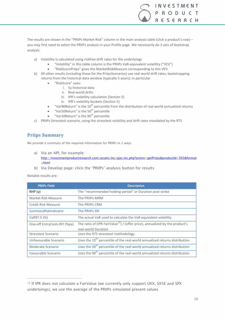
The results are shown in the “PRIIPs Market Risk” column in the main analysis table (click a product’s row) –

you may first need to select the PRIIPs analysis in your Profile page. We necessarily do 3 sets of bootstrap

analysis:

a) Volatility is calculated using riskfree drift rates for the underlyings

“Volatility” in this table column is the PRIIPs VaR-equivalent volatility (“VEV”)

“RiskScorePriips” gives the MarketRiskMeasure corresponding to this VEV b) All other results (including those for the PriipsScenarios) use real world drift rates, bootstrapping

returns from the historical data window (typically 5 years); in particular

“RiskScore” uses: i. 5y historical data

ii. Real world drifts iii. IPR’s volatility calculation (Section 5) iv. IPR’s volatility buckets (Section 5)

“Var90Return” is the 10th

percentile from the distribution of real world annualized returns

“Var50Return” is the 50th

percentile

“Var10Return” is the 90th

percentile c) PRIIPs Stresstest scenario, using the stresstest volatility and drift rates mandated by the RTS

Priips Summary

We provide a summary of the required information for PRIIPs in 2 ways:

a) Via an API, for example:

http://investmentproductresearch.com/assets/inc/ajax.inc.php?action=getPriips&productId=503&format

=html

b) Via Develop page: click the “PRIIPs” analysis button for results

Notable results are:

PRIIPs Field Description

RHP (y) The “recommended holding period” or Duration post-strike

Market Risk Measure The PRIIPs MRM

Credit Risk Measure The PRIIPs CRM

SummaryRiskIndicator The PRIIPs SRI

VaR97.5 (%) The actual VaR used to calculate the VaR equivalent volatility

One-off EntryCosts RIY (%pa) The ratio of (IPR FairValue12

) / (offer price), annualized by the product’s

real-world Duration Stresstest Scenario Uses the RTS stresstest methodology

Unfavourable Scenario Uses the 10th

percentile of the real-world annualized returns distribution

Moderate Scenario Uses the 50th

percentile of the real-world annualized returns distribution

Favourable Scenario Uses the 90th

percentile of the real-world annualized returns distribution

12 If IPR does not calculate a FairValue (we currently only support UKX, SX5E and SPX

underlyings), we use the average of the PRIIPs simulated present values

21

Tables and Charts

PAYOFF ANALYSIS TABLE

We calculate the probability of each event and the return that an investor would receive through a product’s life under each scenario

For callable products we calculate the chance of early maturity at each call date. We also calculate the probability of the product reaching full term. At maturity we calculate the chance that any barrier has been breached.

Where products offer a conditional coupon or a coupon that accumulates over time, we calculate the chance that the coupon is paid, and the amount that an investor can expect

CHARTS

All-products scatter chart The main Listing scatter chart features:

An “efficient frontier” of sorts - a straight line connecting 6y GBP swaps with UK equities (total return) held 6y

Only displayed products are plotted, so you can use the various criteria in the SearchCriteria box isolate the products you want

Customize X and Y axes on your Profile page

Hovering over a plotted point gives tooltip information, and clicking it takes you to the Listing entry for that product (and magnifies that point for easier identification)

Per-product charts Our website provides each product with the following charts:

Historic Back-Test

22

This is the Historic Back-test analysis (described earlier) displayed in chart form.

Future Stress-Test

This is the Future Stress-test analysis (described earlier) displayed in chart form.

Outlook

23

This shows Historic Back-test information:

- Index series: scaled to 1.0 on StrikeDate

- Payoffs: payoff13

for a product started on each date, plotted at that start date

- WorstIndex: performance of worst index over full maturity starting on each date, plotted at that start date

Additional charts The following charts can be made available on request:

Benchmark Comparison

We compare the product's gains and losses with that of a benchmark asset held 6y. The right hand box represents the product's expected conditional gains and the left hand box losses. The height of each box is it’s

13 1.2 for example means a final value of 120%

24

the expected conditional (annualised) return. The width of each box represents its probability. The corresponding values for the benchmark are the wireframe boxes. The points within each box are at their expected (unconditional) returns, i.e. expected Conditional Return times probability. The smaller points are for the benchmark.

This chart allows an investor to visualise the risk and return trade-off for this product versus a benchmark investment. In this instance it is clear that compared with an investment in a portfolio of 40% UK equity, 60% global bonds the product offers the following

- A similar chance of making a profit

- The conditional profit is somewhat higher

- A similar chance of making a loss

- But the conditional loss is much larger

Peer Comparison

We compare the product's expected gains and losses with the best in the same category (those with the most efficient gain to loss ratio).

This is a standard risk/ return efficient frontier chart. Products placed in the North East corner of this chart will have a better risk/return ratio than products at the bottom right. If one product is placed above another it offers a greater return for a similar level of risk. If it placed to the left, it offers less risk for the same level of expected returns. We automatically select 5 other products for comparison based on the product type.

Product Potential Payoffs, Triggers, Barriers

25

We plot the product's:

- Potential payoffs at different points in its life (blue dots)

- Barriers (green dots) – levels which the underlyings must reach for the corresponding

contingent payoff to be made

- Triggers (red dots) – levels which, if reached, trigger potential contingent payoffs,

such as a down-and-in put.

We also plot historical levels for the underlyings, normalised to 1 on the product’s strike date

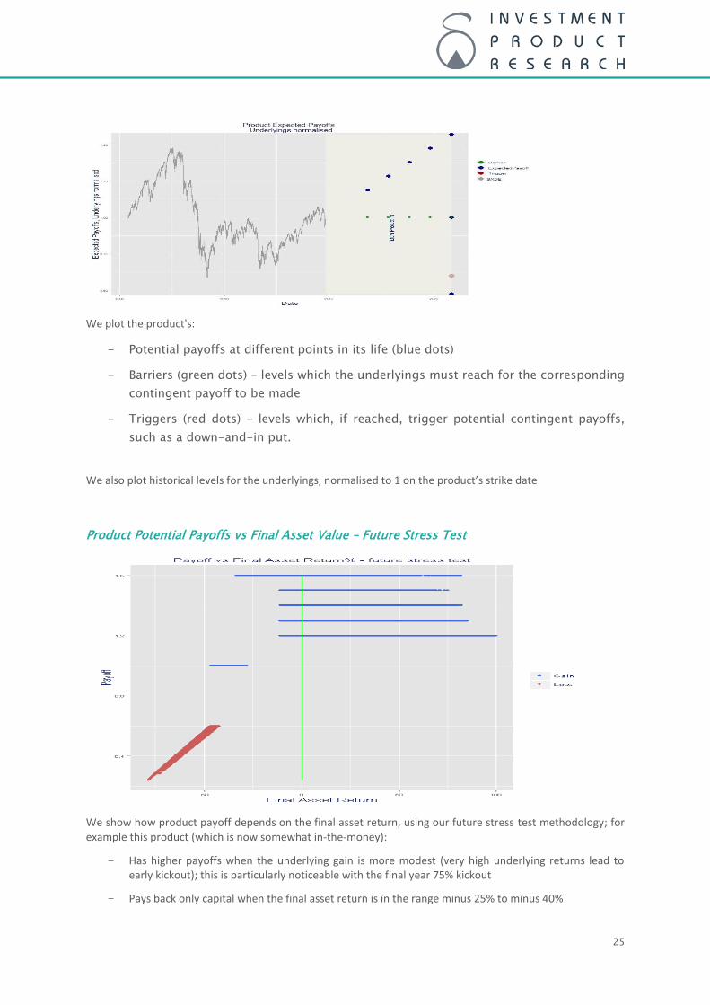
Product Potential Payoffs vs Final Asset Value – Future Stress Test

We show how product payoff depends on the final asset return, using our future stress test methodology; for example this product (which is now somewhat in-the-money):

- Has higher payoffs when the underlying gain is more modest (very high underlying returns lead to early kickout); this is particularly noticeable with the final year 75% kickout

- Pays back only capital when the final asset return is in the range minus 25% to minus 40%

26

- Loses capital only when the final asset return is below minus 40%, losing 40% when the final asset return is -40% and further 1-for-1 losses at lower levels

Distribution of Annualised Returns – Future Stress Test

From the results of our future stress test, we plot the distribution of annualised returns, using 1% return buckets; for this product:

- The significant 12% return bucket reflects kickout in year2

- Lower returns reflect kickouts in other years

- Zero return represents products which do not kickout and where the 60% trigger is not met

- The negative returns reflect products where the 60% trigger is met if the product did not kickout

27

Appendix A – detailed example of volatility calculation

Consider a synthetic zero product, with the following payoffs at maturity

Probability Payoff

80% 1.10

10% 1.00

4% 0.85

3% 0.80

2% 0.75

1% 0.70

The average annualized return is 5.8% and the traditional volatility using all the outcomes

would be 10.6%. The IPR volatility however, concentrating more on potential losses, is

16.1%. Here is how distributions of return, based on these different volatilities compare:

28

This information has been prepared solely for information purposes and is not an offer to buy or sell or a solicitation of an offer to buy or sell any investment offered by Investment Product Research.

Investment Product Research has used historical information in order to provide an illustration of how certain parameters may have performed over a defined period. This presentation may also contain certain performance data based on back-testing, i.e., calculations of the hypothetical performance of a strategy, index or asset as if it had actually existed during a defined period of time. The scenarios, simulations, development expectations and forecasts contained in this presentation are for illustrative purposes only.

The information is based on or derived from information generally available to the public from sources believed to be reliable. No representation or warranty can be given with respect to the accuracy or completeness of the information. We do not undertake to update this information.

Investment Product Research Limited and its affiliates disclaim any and all liability relating to this information, including without limitation any express or implied representations or warranties for statements contained in, and omissions from, this information. Additional information is available on request.

Investment Product Research Limited does not give investment, tax, accounting and legal or regulatory advice and investors should consult with their professional advisers.

Investment Product Research Limited Email support@investmentproductresarch.com

Web http://investmentproductresearch.com