structures 4 lecture notes - university of...
TRANSCRIPT
University of Bath Department of Architecture & Civil Engineering Page 1 of 28
Structures 4 lecture notes
Buckling
Buckling calculations are very difficult except for a few special cases,
and so numerical methods on a computer are almost invariably used in
practice for buckling modes involving plates, shells and assemblies of
beams and columns. Single columns and beams aren’t too bad.
The compression flange of a beam acts more or less like a column
except that the torsional and warping resistance are involved.
However the simple special cases are still worth examining because
they tell us what to look for in a numerical analysis.
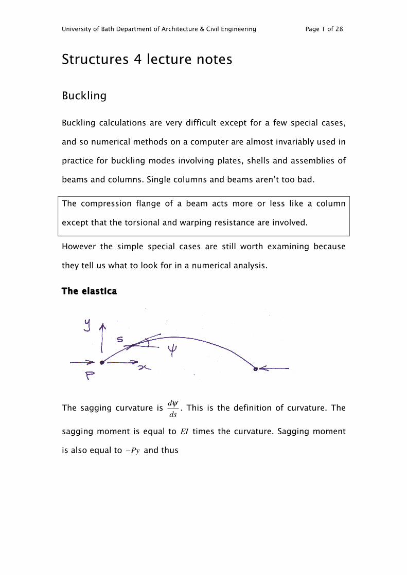
The elastica
The sagging curvature is dψds
. This is the definition of curvature. The
sagging moment is equal to EI times the curvature. Sagging moment
is also equal to −Py and thus
University of Bath Department of Architecture & Civil Engineering Page 2 of 28
M = EI dψds
= −Py = −P sinψ dss=0
s
∫
EI d2ψds2
= −Psinψ
EI dψds
d 2ψds2
= −Psinψ dψds
EI 12
dψds
⎛⎝⎜
⎞⎠⎟2
= P cosψ − cosψ 0( )
where ψ 0 is the value of ψ at s = 0 .
Hence we have
EI 12
dψds
⎛⎝⎜
⎞⎠⎟2
= P cosψ − cosψ 0( )
s = EI2P
dψcosψ − cosψ 0ψ =ψ 0
ψ
∫.
If we write ψ = 2θ , cosψ = cos2θ =1− 2sin2θ and
s = EI2P
2dθ2 sin2θ0 − sin
2θψ =ψ 0
ψ
∫ = EIPsin2θ0
dθ1− k2 sin2θψ =ψ 0
ψ
∫
k = 1sinθ0
.
This is an incomplete elliptic integral of the first kind, - see
http://en.wikipedia.org/wiki/Elliptic_integral
This means that it cannot be evaluated using elementary functions –
trigonometric functions, hyperbolic functions etc.
Alternative derivation:

University of Bath Department of Architecture & Civil Engineering Page 3 of 28
tanψ = dydx
sec2ψ dψds
= d2ydx2
dxds
= d2ydx2
cosψ
dψds
=
d 2ydx2sec3ψ
=
d 2ydx2
1+ tan2ψ( )32
=
d 2ydx2
1+ dydx
⎛⎝⎜
⎞⎠⎟2⎛
⎝⎜⎞
⎠⎟
32
Thus
EI d2ydx2
1+ dydx
⎛⎝⎜
⎞⎠⎟2⎛
⎝⎜⎞
⎠⎟
32
+ Py = 0
EI dydx
d 2ydx2
1+ dydx
⎛⎝⎜
⎞⎠⎟2⎛
⎝⎜⎞
⎠⎟
32
+ Py dydx
= 0
EI
1+ dydx
⎛⎝⎜
⎞⎠⎟ 0
2− EI
1+ dydx
⎛⎝⎜
⎞⎠⎟2+ 12Py2 = 0
We can carry on, but we will get stuck again with an elliptic integral.
However, if we assume that dydx
is small,
1
1+ dydx
⎛⎝⎜
⎞⎠⎟2≈ 1
1+ 12
dydx
⎛⎝⎜
⎞⎠⎟2 ≈1−
12
dydx
⎛⎝⎜
⎞⎠⎟2
so that EI dydx
⎛⎝⎜
⎞⎠⎟2
− dydx
⎛⎝⎜
⎞⎠⎟ 0
2⎛
⎝⎜⎞
⎠⎟+ Py2 = 0 .
This is satisfied by
University of Bath Department of Architecture & Civil Engineering Page 4 of 28
y = Bsin PEIx
⎛⎝⎜
⎞⎠⎟
dydx
= B PEIcos P
EIx
⎛⎝⎜
⎞⎠⎟
dydx
⎛⎝⎜
⎞⎠⎟ 0
= B PEI
.
This gives the Euler column formula,
P = π 2EIL2 = π 2EA
Lr
⎛⎝⎜
⎞⎠⎟
2
A = cross-sectional areaI = Ar2
r = radius of gyrationLr= slenderness ratio
.
For columns other than pin-ended columns, L is the effective
length. For cantilever columns the effective length is more than twice
the actual length, depending on how stiff the moment connection at
the base is.
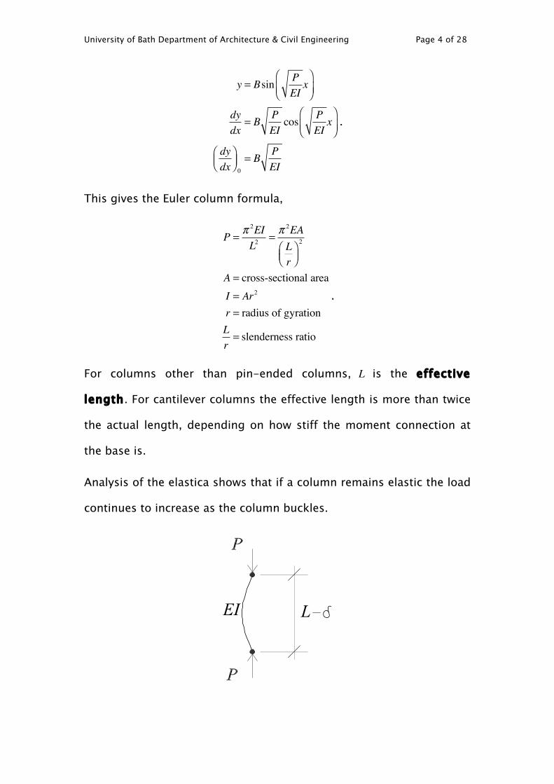
Analysis of the elastica shows that if a column remains elastic the load
continues to increase as the column buckles.

University of Bath Department of Architecture & Civil Engineering Page 5 of 28
The above figure shows a buckled pin ended column of length L and
bending stiffness EI . The column is initially perfectly straight. The
relationship between the buckling load and the shortening due to
bending is PPEuler
= 1+ δ2L
where PEuler =π 2EIL2
is the Euler buckling load.
This formula is obtained using complete elliptic integrals as described
in §2.7 of Timoshenko and Gere, Theory of Elastic Stability and applies
for small values of δL
.
However, it can be shown that for the truss column below that the load
F decreases with deflection (see question 3 in the 2013-14 Structures
4 exam). This is because as the truss deflects the buckled member
attracts more than its fair share of the load.

University of Bath Department of Architecture & Civil Engineering Page 6 of 28
Perry Robinson formula
See the A history of the safety factors by Alasdair N. Beal, The
Structural Engineer 89 (20) 18 October 2011,
http://anbeal.co.uk/TSE2011HistoryofSafetyFactors.pdf
for a fascinating discussion of safety factors including the Perry
Robertson formula.
Assume column has an initial bend, y = ζLsin π xL
⎛⎝⎜
⎞⎠⎟ (note that ζ is
dimensionless) and that dydx
is SMALL. Then the sagging moment,
M = EI × change of curvature = EI d 2ydx2 −
d 2
dx2 ζLsin π xL
⎛⎝⎜
⎞⎠⎟
⎛⎝⎜
⎞⎠⎟
⎛⎝⎜
⎞⎠⎟= −Py
EI d2ydx2 + Py = −EIζL π
2
L2 sin π xL
⎛⎝⎜
⎞⎠⎟
Try solution y = Bsin π xL
⎛⎝⎜
⎞⎠⎟ then
−EIBπ2
L2sin π x
L⎛⎝⎜
⎞⎠⎟ + PBsin
π xL
⎛⎝⎜
⎞⎠⎟ = −EIζL π
2
L2sin π x
L⎛⎝⎜
⎞⎠⎟
B =EIζL π
2
L2
EI π2
L2− P
= ζL
1− Pπ 2EIL2
.
The maximum stress is equal to
University of Bath Department of Architecture & Civil Engineering Page 7 of 28
σ max =PA+ MZ
= PA+ PBZ
= PA+
PLζZ
1− Pπ 2EIL2
= PA+
PALAζZ
1− PPEuler
.
Z = Ic
is the section modulus.
If we set I = Ar2 , Z = Ic= Ar2
c σ = P
A, σ max =σ y and
σ Euler =PEulerA
= π 2EIAL2
= π 2ELr
⎛⎝⎜
⎞⎠⎟2 , then we have
σ y =σ + θσ
1− σσ Euler
.
in which θ = LAζZ
= Lcζr2
.
Therefore
σ Euler −σ( ) σ y −σ( ) +θσ Eulerσ = 0
σ 2 − σ y + 1+θ( )σ Euler( )σ +σ yσ Euler = 0.
σ = 12σ y + 1+θ( )σ Euler( )− 12 σ y + 1+θ( )σ Euler( )2 − 4σ yσ Euler
= 12σ y + 1+θ( )σ Euler( )− 12 σ y + 1+θ( )σ Euler( )2 − 4 1+θ( )σ yσ Euler + 4θσ yσ Euler
= 12σ y + 1+θ( )σ Euler( )− 12 σ y − 1+θ( )σ Euler( )2 + 4θσ yσ Euler
.
When θ = 0 ,
σ = 12σ y +σ Euler( )− 1
2σ y −σ Euler
=σ y or σ Euler
.
University of Bath Department of Architecture & Civil Engineering Page 8 of 28
Note that σ Euler =σ y when π 2ELr
⎛⎝⎜
⎞⎠⎟2 =σ y so that L
r= π E
σ y
.
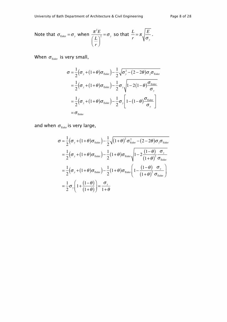
When σ Euler is very small,
σ ! 12σ y + 1+θ( )σ Euler( )− 12 σ y
2 − 2 − 2θ( )σ yσ Euler
= 12σ y + 1+θ( )σ Euler( )− 12σ y 1− 2 1−θ( )σ Euler
σ y
!12σ y + 1+θ( )σ Euler( )− 12σ y 1− 1−θ( )σ Euler
σ y
⎡
⎣⎢
⎤
⎦⎥
!σ Euler
and when σ Euler is very large,
σ ! 12σ y + 1+θ( )σ Euler( )− 12 1+θ( )2σ Euler
2 − 2 − 2θ( )σ yσ Euler
= 12σ y + 1+θ( )σ Euler( )− 12 1+θ( )σ Euler 1− 2
1−θ( )1+θ( )2
σ y
σ Euler
!12σ y + 1+θ( )σ Euler( )− 12 1+θ( )σ Euler 1−
1−θ( )1+θ( )2
σ y
σ Euler
⎛
⎝⎜⎞
⎠⎟
= 12σ y 1+
1−θ( )1+θ( )
⎛⎝⎜
⎞⎠⎟=
σ y
1+θ

University of Bath Department of Architecture & Civil Engineering Page 9 of 28
Perry-Robertson graphs with Eσ y
= 1000 and θ = 0, 0.01, 0.1 and 1.
See http://en.wikipedia.org/wiki/Perry_Robertson_formula
This is the basis for column design.
Timoshenko or Cosserat column

University of Bath Department of Architecture & Civil Engineering Page 10 of 28
The figure on the left a shows the buckling of a battened or Vierendeel
column. The deformation has been exaggerated so that the deflected
shape can be seen.
The figure on the right shows a detail of two bays in which the circles
show the assumed points of contraflexure half way along the members.
If the column is treated as a Timoshenko or Cosserat beam, the
differential equations describing deformation of the column are
M = Py = −EIcompositeddx
dydx
−θ⎛⎝⎜
⎞⎠⎟
kθ = F = P dydx
in which x is the vertical coordinate along the column, y is the lateral
displacement of the column, M is the overall bending moment, P is
the overall axial load and F is the overall shear force. Icomposite is the
fully composite second moment of area and k is the shear stiffness of
the column.
Hence
EIcompositeddx
dydx
− Pkdydx
⎛⎝⎜
⎞⎠⎟ + Py = 0
EIcomposite 1−Pk
⎛⎝⎜
⎞⎠⎟d 2ydx2
+ Py = 0.
If the column is pin-ended and its length is length L , the differential
equation is satisfied by
y = Bsinπ xL
if
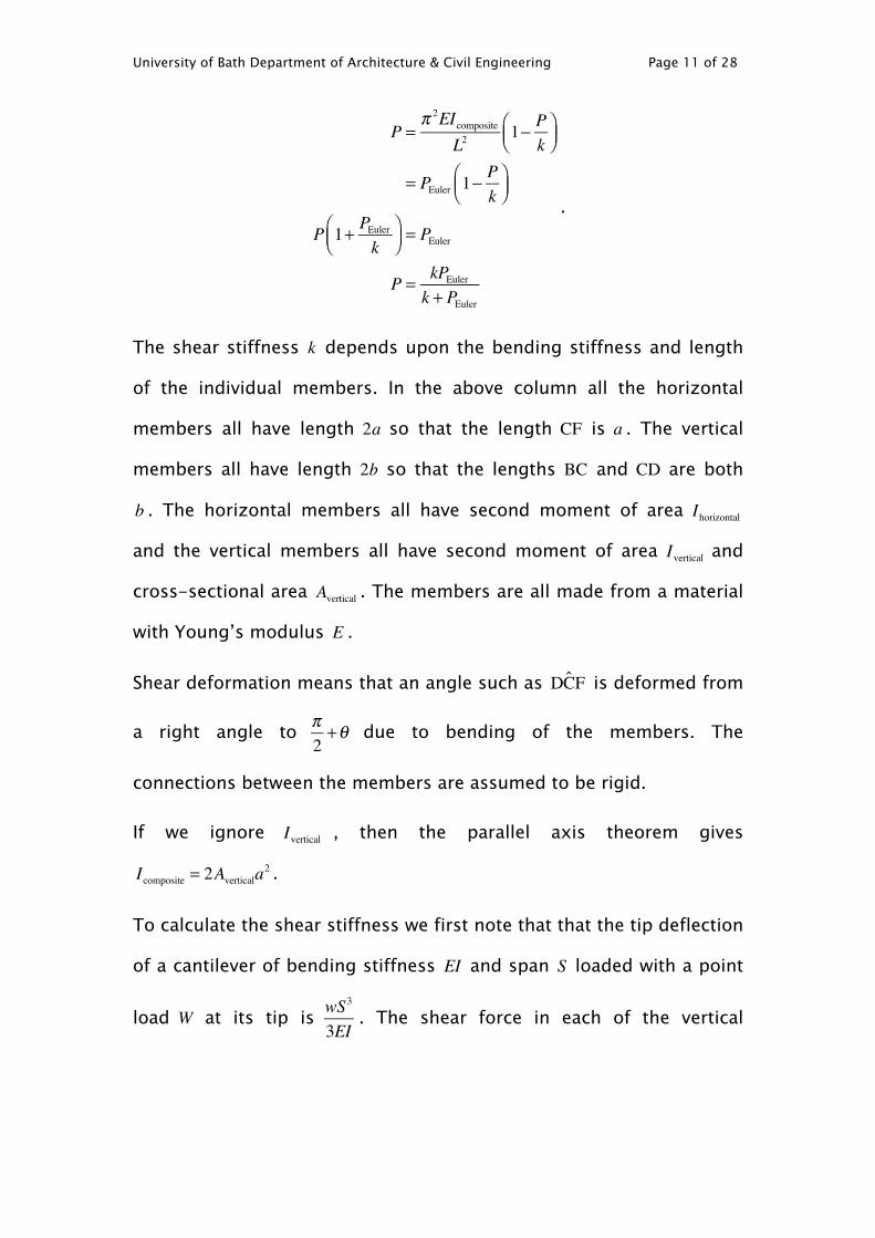
University of Bath Department of Architecture & Civil Engineering Page 11 of 28
P =π 2EIcomposite
L21− P
k⎛⎝⎜
⎞⎠⎟
= PEuler 1−Pk
⎛⎝⎜
⎞⎠⎟
P 1+ PEulerk
⎛⎝⎜
⎞⎠⎟ = PEuler
P = kPEulerk + PEuler
.
The shear stiffness k depends upon the bending stiffness and length
of the individual members. In the above column all the horizontal
members all have length 2a so that the length CF is a . The vertical
members all have length 2b so that the lengths BC and CD are both
b . The horizontal members all have second moment of area Ihorizontal
and the vertical members all have second moment of area Ivertical and
cross-sectional area Avertical . The members are all made from a material
with Young’s modulus E .
Shear deformation means that an angle such as DCF is deformed from
a right angle to π2+θ due to bending of the members. The
connections between the members are assumed to be rigid.
If we ignore Ivertical , then the parallel axis theorem gives
Icomposite = 2Averticala2 .
To calculate the shear stiffness we first note that that the tip deflection
of a cantilever of bending stiffness EI and span S loaded with a point
load W at its tip is wS3
3EI. The shear force in each of the vertical

University of Bath Department of Architecture & Civil Engineering Page 12 of 28
members is F2
and the shear force in the horizontal members is
2 F2b
a= Fba
. Thus the shear deformation is
θ =
F2b3
3EIvertical
⎛
⎝
⎜⎜⎜
⎞
⎠
⎟⎟⎟
b+
Fbaa3
3EIhorizontal
⎛
⎝
⎜⎜⎜
⎞
⎠
⎟⎟⎟
a= Fb2
6EIvertical+ Fab3EIhorizontal
.
Hence k = 1b2
6EIvertical+ ab3EIhorizontal
.
Buckling of plates and shells
See, for example, Don O. Brush and Bo O. Almroth, Buckling of Bars,
Plates and Shells, McGraw-Hill, New York 1975.
Plates behave fairly well when they buckle, the load usually does not
drop off dramatically and may increase after buckling. On the other
hand shells, including axially compressed cylinders, can be very
imperfection sensitive so they collapse at a much smaller load than the
eigenvalue buckling load - see
Hunt, G. W., 2011. Reflections and symmetries in space and time. IMA
Journal of Applied Mathematics, 76 (1), pp. 2-26.
http://imamat.oxfordjournals.org/content/76/1/2

University of Bath Department of Architecture & Civil Engineering Page 13 of 28
Simply supported flat plate
Image from Brush and Almroth, Buckling of Bars, Plates and Shells
For a straight beam we have
EI d2vdx2
+ Pv = 0
EI d4vdx4
+ P d2vdx2
= 0
where v is the displacement in the y direction. The corresponding
equation for a flat plate is
D ∂4w∂x4
+ 2 ∂4w∂x2 ∂y2
+ ∂4w∂y4
⎛⎝⎜
⎞⎠⎟+σ x
∂2w∂x2
= 0
D = Et 3
12 1−υ 2( )
in which it is assumed that that there is only a membrane stress σ x in
the x direction. Membrane stress has units force per unit width. w is
the displacement in the z direction, t is the plate thickness and υ is
Poisson’s ratio. D is the bending stiffness per unit width and it
replaces the E bd3
12 for a rectangular beam.

University of Bath Department of Architecture & Civil Engineering Page 14 of 28
Let us suppose that the plate is simply supported along y = 0 and y = b
and that it is long in the x direction. The differential equation is
satisfied and the y = 0 and y = b boundary conditions are satisfied by
w = Asin 2π xλsinπ y
b
if
σ x2πλ
⎛⎝⎜
⎞⎠⎟2
= D 2πλ
⎛⎝⎜
⎞⎠⎟4
+ 2 2πλ
⎛⎝⎜
⎞⎠⎟2 πb
⎛⎝⎜
⎞⎠⎟2
+ πb
⎛⎝⎜
⎞⎠⎟4⎛
⎝⎜⎞
⎠⎟= D 2π
λ⎛⎝⎜
⎞⎠⎟2
+ πb
⎛⎝⎜
⎞⎠⎟2⎛
⎝⎜⎞
⎠⎟
2
so that
σ x = D2πλ
⎛⎝⎜
⎞⎠⎟ +
πb
⎛⎝⎜
⎞⎠⎟2
2πλ
⎛⎝⎜
⎞⎠⎟
⎛
⎝
⎜⎜⎜⎜
⎞
⎠
⎟⎟⎟⎟
2
which is minimum when
dσ x
dλ= −2D 2π
λ⎛⎝⎜
⎞⎠⎟ +
πb
⎛⎝⎜
⎞⎠⎟2
2πλ
⎛⎝⎜
⎞⎠⎟
⎛
⎝
⎜⎜⎜⎜
⎞
⎠
⎟⎟⎟⎟
1−
πb
⎛⎝⎜
⎞⎠⎟2
2πλ
⎛⎝⎜
⎞⎠⎟2
⎛
⎝
⎜⎜⎜⎜
⎞
⎠
⎟⎟⎟⎟
2πλ 2 = 0
λ = 2b
.
Thus the buckling membrane stress is
σ x = 4Dπb
⎛⎝⎜
⎞⎠⎟2
.
Simple single degree of freedom models
These will be introduced in lectures, with particular reference to post-
buckled stability and imperfection sensitivity. In particular the
University of Bath Department of Architecture & Civil Engineering Page 15 of 28
difference between non-linear and linear (eigenvalue) buckling will be
emphasised.
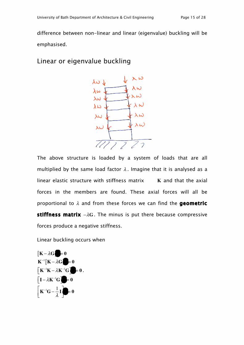
Linear or eigenvalue buckling
The above structure is loaded by a system of loads that are all
multiplied by the same load factor λ . Imagine that it is analysed as a
linear elastic structure with stiffness matrix K and that the axial
forces in the members are found. These axial forces will all be
proportional to λ and from these forces we can find the geometric
stiffness matrix −λG . The minus is put there because compressive
forces produce a negative stiffness.
Linear buckling occurs when
K − λG[ ]δ = 0
K−1 K − λG[ ]δ = 0
K−1K − λK−1G⎡⎣ ⎤⎦δ = 0
I − λK−1G⎡⎣ ⎤⎦δ = 0
K−1G − 1λI⎡
⎣⎢⎤⎦⎥δ = 0
.

University of Bath Department of Architecture & Civil Engineering Page 16 of 28
We are only interested in the lowest buckling load for which the load
factor λ is equal to one over the highest eigenvalue of K−1G . The
corresponding eigenvector gives the mode shape.
Note the similarity to natural frequencies and mode shapes. Buckling
corresponds to the natural frequency becoming zero.
Note that linear eigenvalue buckling analysis gives no information
about imperfection sensitivity.
Therefore non-linear buckling analysis should always be done if there
is any question of imperfection sensitivity.
The P − Δ effect refers to the moment caused by side-sway of a
column. It is sometimes not clear what is meant by P − Δ analysis in a
piece of software regarding linear or non-linear. Note that rotation is
not a vector unless it is small and this assumption is often made even
in so called non-linear analysis.

University of Bath Department of Architecture & Civil Engineering Page 17 of 28
Lagrange's Equations of Motion
Kinetic energy = T = 12
Mijδ i δ j
j=1
n
∑i=1
n
∑ = 12δTMδ where n is the number of
degrees of freedom. The Mij are functions of the δ ’s only.
dTdt
= 12
Mij!!δ i!δ j +Mij
!δ i!!δ j +
∂Mij
∂δ k
!δ i!δ j!δ k
k=1
n
∑⎛⎝⎜
⎞⎠⎟j=1
n
∑i=1
n
∑
= !δ i
Mij +M ji( )2
!!δ j +12
∂M jk
∂δ i
+∂Mkj
∂δ i
⎛⎝⎜
⎞⎠⎟
2!δ j!δ k
k=1
n
∑⎛
⎝
⎜⎜⎜⎜
⎞
⎠
⎟⎟⎟⎟
j=1
n
∑
⎡
⎣
⎢⎢⎢⎢
⎤
⎦
⎥⎥⎥⎥
i=1
n
∑
= !δ i
Mij +M ji( )2
!!δ j +
∂M jk
∂δ i
+∂Mkj
∂δ i
⎛⎝⎜
⎞⎠⎟
2!δ j!δ k
k=1
n
∑ − 12
∂M jk
∂δ i
+∂Mkj
∂δ i
⎛⎝⎜
⎞⎠⎟
2!δ j!δ k
k=1
n
∑⎛
⎝
⎜⎜⎜⎜
⎞
⎠
⎟⎟⎟⎟
j=1
n
∑
⎡
⎣
⎢⎢⎢⎢
⎤
⎦
⎥⎥⎥⎥
i=1
n
∑
= !δ iddt
∂T∂ !δ i
⎛⎝⎜
⎞⎠⎟− ∂T∂δ i
⎛
⎝⎜⎞
⎠⎟⎡
⎣⎢⎢
⎤
⎦⎥⎥i=1
n
∑
If U is the strain energy and G is the gravitational potential energy, by
conservation of energy,
0 = ddt
T +U +G( ) = δ iddt
∂T∂ δ i
⎛⎝⎜
⎞⎠⎟− ∂T∂δ i
+ ∂U∂δ i
+ ∂G∂δ i
⎛
⎝⎜⎞
⎠⎟⎡
⎣⎢⎢
⎤
⎦⎥⎥i=1
n
∑
This equation applies for arbitrary δ i and therefore
ddt
∂T∂ δ i
⎛⎝⎜
⎞⎠⎟− ∂T∂δ i
+ ∂U∂δ i
+ ∂G∂δ i
= 0 .
These are Lagrange’s equations of motion and apply for i =1 to n .
University of Bath Department of Architecture & Civil Engineering Page 18 of 28
Verlet integration
If the equations of motion can be rearranged so that:
δ1 = q1 δ1,δ2,...,δn, δ1, δ2,..., δn, p1, p2,..., pn( )δ2 = q2 δ1,δ2,...,δn, δ1, δ2,..., δn, p1, p2,..., pn( )....
δn = qn δ1,δ2,...,δn, δ1, δ2,..., δn, p1, p2,..., pn( )
in which the loads p1, p2,..., pn are known values of time and if we also
know the initial values of δ1,δ2,...,δn, δ1, δ2,..., δn , then we can step
through time updating values as follows:
δ1 = δ1 + δ1Δtδ2 = δ2 + δ2Δt....
δn = δn + δnΔt
and
δ1 = δ1 + δ1Δt
δ2 = δ2 + δ2Δt....
δn = δn + δnΔt
.
There are a number of essentially similar ‘explicit’ methods like this
with names such as Verlet Integration, Störmer's method, Gauss–Seidel
and dynamic relaxation.
University of Bath Department of Architecture & Civil Engineering Page 19 of 28
Definitions of some terms used for non-
aeroelastic vibrations
Note that single degree of freedom systems are very important
because multidegree of freedom systems can be reduced to uncoupled
single degree of freedom systems using modal analysis and the
orthogonality conditions discussed in lectures – this is ignoring the
coupling due to damping.
Summary of results
In order to solve the equations
Mδ••+Dδ
•+Kδ = p
for a system with n degrees of freedom, we write δ = fr t( )Δ rr=1
n
∑ where
Δ r are the eigenvectors of K−1M .
If we ignore coupling due to damping,
mr fr••+ λr fr
•+ kr fr = pr t( )mr = Δ r
TMΔ r
kr = Δ rTKΔ r
λr = 2c krmr
pr t( ) = Δ rTp
c = non-dimensional damping ratio
which is the equation for a single degree of freedom system.

University of Bath Department of Architecture & Civil Engineering Page 20 of 28
Single degree of freedom system
Figure 1
Figure 1 shows a typical ‘random’ load, p t( ).
The mean value of p t( ) is µp =1T
p t( )dt−T
2
T2
∫ as T →∞ .
The auto-correlation function is Rpp τ( ) = 1T
p t( ) p t +τ( )dt−T
2
T2
∫ as T →∞ .
The auto-correlation function of p t( ) minus its mean is
1T
p t( )− µp⎡⎣ ⎤⎦ p t +τ( )− µp⎡⎣ ⎤⎦dt−T
2
T2
∫ as T →∞
= Rpp τ( )− µp2.
The mean-square spectral density is
φpp ω( ) = 12π
Rpp τ( )− µp2⎡⎣ ⎤⎦e
−iωτ dτ−∞
∞
∫ = 12π
Rpp τ( )− µp2⎡⎣ ⎤⎦cos ωτ( )dτ
−∞
∞
∫ . Here
ω = 2π × frequency .
From the theory of Fourier transforms,
Rpp τ( ) = µp2 + φpp ω( )eiωτ dω
−∞
∞
∫ = µp2 + φpp ω( )cos ωτ( )dω
−∞
∞
∫ .
University of Bath Department of Architecture & Civil Engineering Page 21 of 28
Note that µp , Rpp τ( ) and φ pp ω( ) are all real, and Rpp −τ( ) = Rpp τ( ) and
φ pp −ω( ) = φ pp ω( ).
σ p is the standard deviation of p t( ) which is defined as
σ p2 = 1
Tp t( )− µp⎡⎣ ⎤⎦ p t( )− µp⎡⎣ ⎤⎦dt
−T2
T2
∫ as T →∞
= Rpp 0( )− µp2 = φpp ω( )dω
−∞
∞
∫
The mean-square spectral density tells us about the amount of
‘energy’ at different frequencies, but gives no information about the
relative phase.
ψ p is the root mean square (rms) value of p t( ) and
ψ p2 = µp
2 +σ p2 = Rpp 0( ).
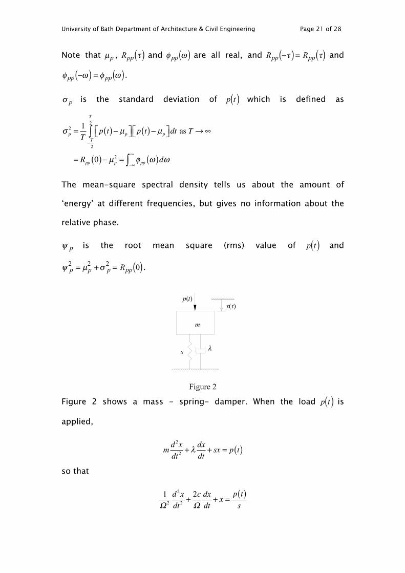
Figure 2
Figure 2 shows a mass - spring- damper. When the load p t( ) is
applied,
m d 2xdt2
+ λ dxdt
+ sx = p t( )
so that
1Ω 2
d 2xdt2
+ 2cΩdxdt
+ x =p t( )s
m
p(t)x(t)
s λ

University of Bath Department of Architecture & Civil Engineering Page 22 of 28
where Ω = sm
= 2π × natural frequency and the viscous damping factor,
c = λ2 sm
.
The mean value of x t( ) is µx =µp
s.
The mean-square spectral density of x t( ) is φxx ω( ) =
φpp ω( )s2
⎛⎝⎜
⎞⎠⎟
1− ω 2
Ω 2⎛⎝⎜
⎞⎠⎟
2
+ 2cωΩ
⎛⎝⎜
⎞⎠⎟2
.
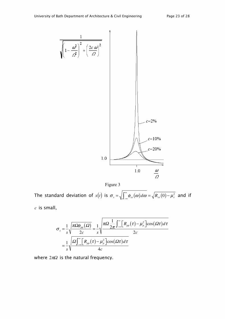
Figure 3 shows plots of 1
1− ω 2
Ω 2⎛⎝⎜
⎞⎠⎟
2
+ 2cωΩ
⎛⎝⎜
⎞⎠⎟2
.
University of Bath Department of Architecture & Civil Engineering Page 23 of 28
Figure 3
The standard deviation of x t( ) is σ x = φxx ω( )dω−∞
∞
∫ = Rxx 0( )− µx2 and if
c is small,
σ x =1s
πΩφpp Ω( )2c
= 1s
πΩ 12π
Rpp τ( )− µp2⎡⎣ ⎤⎦cos Ωτ( )dτ
−∞
∞
∫2c
= 1s
Ω Rpp τ( )− µp2⎡⎣ ⎤⎦cos Ωτ( )dτ
−∞
∞
∫4c
where 2πΩ is the natural frequency.
University of Bath Department of Architecture & Civil Engineering Page 24 of 28
The ‘dynamic magnification factor’ is πΩφpp Ω( )2cσ p
2 . Note that this
dynamic magnification factor applies only to the dynamic
component of the load.
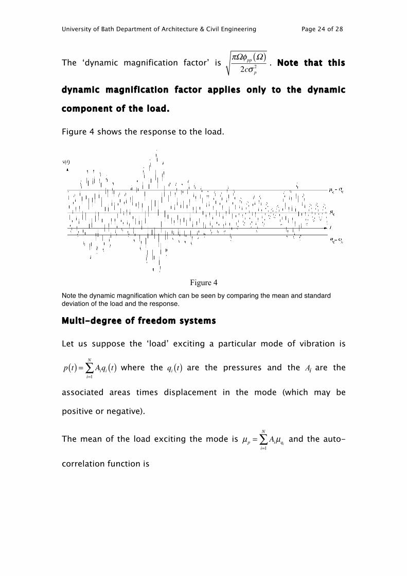
Figure 4 shows the response to the load.
Figure 4
Note the dynamic magnification which can be seen by comparing the mean and standard deviation of the load and the response.
Multi-degree of freedom systems
Let us suppose the ‘load’ exciting a particular mode of vibration is
p t( ) = Aiqi t( )i=1
N
∑ where the qi t( ) are the pressures and the Ai are the
associated areas times displacement in the mode (which may be
positive or negative).
The mean of the load exciting the mode is µp = Aiµqii=1
N
∑ and the auto-
correlation function is
University of Bath Department of Architecture & Civil Engineering Page 25 of 28
Rpp τ( ) = AiAjRqiqj τ( )j=1
N
∑i=1
N
∑
= µp2 + AiAj Rqiqj τ( )− µqi
µqj⎡⎣ ⎤⎦
j=1
N
∑i=1
N
∑
where the cross-correlation,
Rqiqj τ( ) = Rqjqi −τ( ) = 1T
qi t( )qj t +τ( )dt−T
2
T2
∫ as T →∞ .
Again φpp ω( ) = 12π
Rpp τ( )− µp2⎡⎣ ⎤⎦e
−iωτ dτ−∞
∞
∫ .
Note that in general Rqiqj −τ( ) ≠ Rqiqj τ( ) so that cross mean-square
spectral density,
φqiqj ω( ) = φqiqj −ω( ) = φqjqi −ω( ) = 12π
Rqiqj τ( )− µqiµqj
⎡⎣ ⎤⎦e−iωτ dτ
−∞
∞
∫ will be a
complex function.
However in doing the summation φpp ω( ) = AiAjφqiqj ω( )j=1
N
∑i=1
N
∑ , the
imaginary parts will cancel out.
In terms of correlation functions, the response is given by
σ x =1m
AiAj Rqiqj τ( )− µqiµqj
⎡⎣ ⎤⎦j=1
N
∑i=1
N
∑⎛
⎝⎜⎞
⎠⎟cos Ωτ( )dτ
−∞
∞
∫4c
.
A note on Fourier series
For our purposes a stochastic random load can be approximated by
the Fourier series,
p t( ) = µp + 2φpp ωn( )Δω 2 cos ωnt + βp ωn( )( )( )n=1
∞
∑

University of Bath Department of Architecture & Civil Engineering Page 26 of 28
where ωn =
2πnT
and Δω =
2πT
if the period, T , is sufficiently large. Stochastic means
‘governed by the laws of probability’. The autocorrelation function,
Rpp τ( ) = 1T
µp + 2φpp ωn( )Δω 2 cos ωnt + βp ωn( )( )( )n=1
∞
∑⎡⎣⎢
⎤⎦⎥
µp + 2φpp ωn( )Δω 2 cos ωn t +τ( )+ βp ωn( )( )( )n=1
∞
∑⎡⎣⎢
⎤⎦⎥
⎛
⎝
⎜⎜⎜⎜
⎞
⎠
⎟⎟⎟⎟
dt−T
2
T2
∫ as T →∞
= µp2 + 1
T2φpp ωn( )Δω2cos ωn t +τ( )+ βp ωn( )( )cos ωnt + βp ωn( )( )( )
n=1
∞
∑ dt−T
2
T2
∫
= µp2 + 1
T2φpp ωn( )Δω2
cos ωnτ( )cos2 ωnt + βp ωn( )( )−sin ωnτ( )sin ωnt + βp ωn( )( )cos ωnt + βp ωn( )( )
⎛
⎝⎜⎜
⎞
⎠⎟⎟
⎛
⎝⎜⎜
⎞
⎠⎟⎟n=1
∞
∑ dt−T
2
T2
∫
= µp2 + 2φpp ωn( )Δω cos ωnτ( )( )
n=1
∞
∑
= µp2 + 2 φpp ωn( )cos ωnτ( )( )
n=1
∞
∑ Δω
You can also use the Fourier transform, but this seems to cause problems with spectral
densities unless you limit the time to − T2≤ t ≤ T
2.
Duhamel's integral
Duhamel's integral is a bit like Verlet integration, except that it only
applies to linear systems.
The unloaded single degree of freedom system:
m d 2xdt2
+ λ dxdt
+ sx = 0 or 1Ω 2
d 2xdt2
+ 2cΩdxdt
+ x =p t( )s
where
Ω = sm
= 2π × natural frequency and the viscous damping factor,
c = λ2 sm
is satisfied by
University of Bath Department of Architecture & Civil Engineering Page 27 of 28
x = e−cΩt Asin 1− c2( )Ωt( )+ Bcos 1− c2( )Ωt( )( ) . If the mass is stationary and receives an impulse I at t = 0 , then when
t > 0 ,
x = Im
e−cΩt sin 1− c2( )Ωt( )1− c2( )Ω .
Duhamel's integral treats the load as lots of little impulses so that
x = 1m 1− c2( )Ω e−cΩ t−τ( ) sin 1− c2( )Ω t −τ( )( ) p τ( )dτ
0
t
∫ .
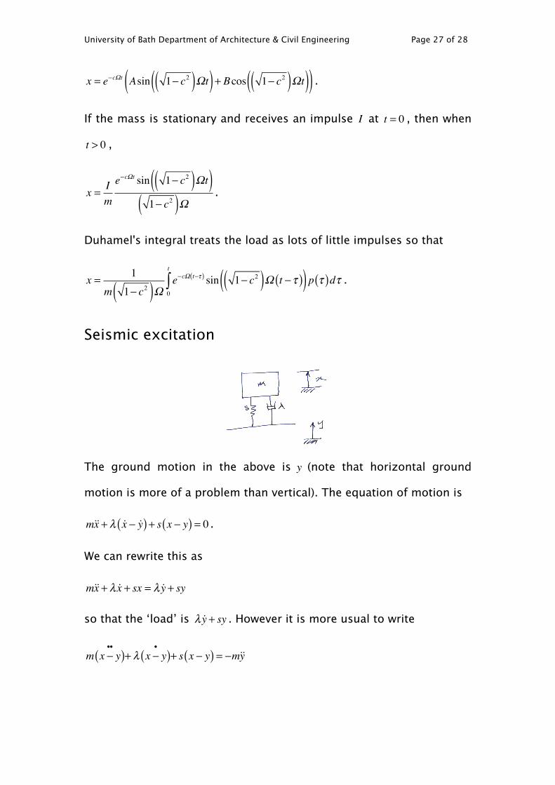
Seismic excitation
The ground motion in the above is y (note that horizontal ground
motion is more of a problem than vertical). The equation of motion is
mx + λ x − y( )+ s x − y( ) = 0 .
We can rewrite this as
mx + λ x + sx = λ y + sy
so that the ‘load’ is λ y + sy . However it is more usual to write
m x − y( )••
+ λ x − y( )•
+ s x − y( ) = −my

University of Bath Department of Architecture & Civil Engineering Page 28 of 28
in which x − y( ) is the motion relative to the ground and it is this
motion which causes the stresses in the structure. The ‘load’ is now
simply −my . This is easy to implement in matrix notation for multi-
degree of freedom systems.
Aeroelasticity
This is discussed in lectures using the example of the Fokker E.V (later
the D-VIII) monoplane (divergence) and the Tacoma Narrows bridge
(single degree of freedom non-classical flutter) - see
http://books.google.co.uk/books?id=DnQOzYDJsm8C&dq=stall+flutt
er+tacoma&source=gbs_navlinks_s
Chris Williams