arX

iv:2

011.

0412

0v2

[gr

-qc]

17

Oct

202

1

Oscillating 4-Polytopal Universe in Regge Calculus

Ren Tsuda1and Takanori Fujiwara

2

1Student Support Center, Chiba Institute of Technology, Narashino 275-0023, Japan2Department of Physics, Ibaraki University, Mito 310-8512, Japan

Abstract

The discretized closed Friedmann–Lemaıtre–Robertson–Walker (FLRW) universe

with positive cosmological constant is investigated by Regge calculus. According to

the Collins–Williams formalism, a hyperspherical Cauchy surface is replaced with reg-

ular 4-polytopes. Numerical solutions to the Regge equations approximate well to the

continuum solution during the era of small edge length. Unlike the expanding poly-

hedral universe in three dimensions, the 4-polytopal universes repeat expansions and

contractions. To go beyond the approximation using regular 4-polytopes we introduce

pseudo-regular 4-polytopes by averaging the dihedral angles of the tessellated regular

600-cell. The degree of precision of the tessellation is called the frequency. Regge

equations for the pseudo-regular 4-polytope have simple and unique expressions for

any frequency. In the infinite frequency limit, the pseudo-regular 4-polytope model

approaches the continuum FLRW universe.

1 Introduction

Regge calculus was proposed in 1961 to formulate Einstein’s general relativity on piecewise

linear manifolds [1, 2]. It is a coordinate-free discrete formulation of gravity, providing a

framework in both classical and quantum studies of gravity [3]. Since Regge calculus is

a highly abstract and abstruse theoretical formalism based on simplicial decomposition of

space-time, further theoretical studies from various viewpoints are to be welcomed. In par-

ticular, exact results such as the Friedmann–Lemaıtre–Robertson–Walker (FLRW) universe

and Schwarzschild space-time in the continuum theory are considered to play the role of a

touchstone in Regge calculus. Thorough investigations on these systems are indispensable

in making Regge calculus practical for use.

Regge calculus has been applied to the four-dimensional closed FLRW universe by Collins

and Williams [4]. They considered regular polytopes (4-polytopes or polychora) as the

Cauchy surfaces of the discrete FLRW universe and used, instead of simplices, truncated

world-tubes evolving from one Cauchy surface to the next as the building blocks of piecewise

linear space-time. Their method, called the Collins–Williams (CW) formalism, is based on

the 3 + 1 decomposition of space-time similar to the well-known Arnowitt–Deser–Misner

(ADM) formalism [5–7]. Recently, Liu and Williams have extensively studied the discrete

FLRW universe [8–10]. They found that a universe with regular 4-polytopes such as the

Cauchy surfaces can reproduce the continuum FLRW universe to a certain degree of precision.

Their solutions agree well with the continuum when the size of the universe is small, whereas

the deviations from the exact results become large for a large universe.

In a previous paper [11], we investigated the three-dimensional closed FLRW universe

with positive cosmological constant by the CW formalism. The main interest there was to

elucidate how Regge calculus reproduces the FLRW universe in the continuum limit. In

three dimensions, a spherical Cauchy surface is replaced with polyhedra. We described the

five types of regular polyhedra on an equal footing by using Schlafli symbols [12]. The

polyhedral universe behaves as the analytic solution of the continuum theory when the size

of the universe is small, while it expands to infinity in a finite time. We further proposed

a geodesic dome model to go beyond the regular polyhedra. The Regge calculus for the

geodesic domes, however, becomes more and more complicated as we better and better ap-

proximate the sphere. To avoid the cumbersome tasks in carrying out Regge calculus for

the geodesic dome models we introduced pseudo-regular polyhedra characterized by frac-

tional Schlafli symbols. Regge equations for the pseudo-regular polyhedron model turned

out to approximate the corresponding geodesic dome universe well. It is worth investigating

whether a similar approach can be extended to higher dimensions.

In this paper we investigate the FLRW universe of four-dimensional Einstein gravity with

a positive cosmological constant within the framework of the CW formalism. We consider all

six types of regular 4-polytopes as the Cauchy surface in a unified way in terms of the Schlafli

2

k = 1 k = 0 k = −1

Λ > 0 a =√

3Λcosh

(√

Λ3t)

a =√

3Λexp

(√

Λ3t)

a =√

3Λsinh

(√

Λ3t)

Λ = 0 no solution a = const. a = t

Λ < 0 no solution no solution a =√

− 3Λsin(√

−Λ3t)

Table 1: Solutions of the Friedmann equations.

symbol and compare the behaviors of the solutions with the analytic result of the continuum

theory. We further propose a generalization of the Regge equations by introducing pseudo-

regular polytopes, which makes the numerical analysis much easier than the conventional

Regge calculus.

This paper is organized as follows: in the next section we set up the regular 4-polytopal

universe in the CW formalism and introduce Regge action. Derivation of the Regge equa-

tions is given in Sect. 3. In the continuum time limit the Regge equations are reduced to

differential equations. Applying the Wick rotation, we arrive at the Regge calculus analog of

the Friedmann equations, describing the evolution of the 4-polytopal universe. This is done

in Sect. 4. In Sect. 5 we solve the differential Regge equations numerically and compare the

scale factors of the 4-polytopal universes with the continuum solution. In Sect. 6 we consider

subdivision of cells of the regular 4-polytopes and propose a pseudo-regular 4-polytopal uni-

verse with a non-integer Schlafli symbol that approaches a smooth three-dimensional sphere

in the continuum limit. Sect. 7 is devoted to summary and discussions. In Appendix A, the

radius of the circumsphere of a regular polytope in any dimensions is considered.

2 Regge action for a regular 4-polytopal universe

We begin with a brief description of the continuum FLRW universe. The continuum action

is given by

S =1

16π

∫

d4x√−g(R − 2Λ). (2.1)

In four dimensions, the Einstein equations have an evolving universe as a solution for the

ansatz

ds2 = −dt2 + a(t)2[

dr2

1− kr2+ r2

(

dθ2 + sin2 θdϕ2)

]

, (2.2)

where a (t) is the so-called scale factor in cosmology. It is subject to the Friedmann equations

a2 =Λ

3a2 − k, a =

Λ

3a. (2.3)

3

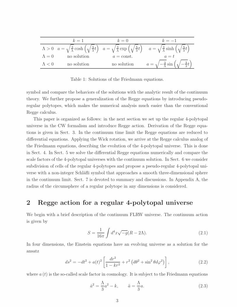
The curvature parameter k = 1, 0,−1 corresponds to space being spherical, Euclidean, or

hyperbolic, respectively. The relations between the solutions and curvature parameter are

summarized in Table 1 with the proviso that the behaviors of the universes are restricted to

expanding at the beginning for the initial condition a(0) = min a(t). Of these, our concern is

the spherical universe with three-dimensional spheres as the Cauchy surfaces. All the time

dependence of the universe is in the scale factor a(t), which expresses the curvature radius

of the Cauchy surface. In Regge calculus we will replace the three-dimensional sphere with

a regular 4-polytope.

Before entering into details of the 4-polytopal universe, let us briefly summarize the

essence of Regge calculus: in Regge calculus, an analog of the Einstein–Hilbert action is

given by the Regge action [13]

SRegge =1

8π

∑

i∈{hinges}εiAi − Λ

∑

i∈{blocks}Vi

, (2.4)

where Ai is the volume of a hinge, εi the deficit angle around the hinge Ai, and Vi the

volume of a building block of the piecewise linear manifold. In four dimensions the hinges

are the lattice planes, or equivalently the faces of the 4-simplices, and Ai is nothing but

the face area. Regge’s original derivation is concerned with a simplicial lattice, so that it

describes the gravity as simplicial geometry. In fact this formalism can easily be generalized

to arbitrary lattice geometries. We can fully triangulate the non-simplicial flat blocks by

adding extra hinges with vanishing deficit angles without affecting the Regge action.

The fundamental variables in Regge calculus are the edge lengths li. Varying the Regge

action with respect to li, we obtain the Regge equations

∑

i∈{hinges}εi∂Ai

∂lj− Λ

∑

i∈{blocks}

∂Vi∂lj

= 0. (2.5)

Note that there is no need to carry out the variation of the deficit angles owing to the Schlafli

identity [14, 15]

∑

i∈{hinges}Ai

∂εi∂lj

= 0. (2.6)

We now turn to 4-polytopal universes. Following the CW formalism, we replace the

hyperspherical Cauchy surface by a regular 4-polytope. It would be helpful to begin with a

description of regular 4-polytopes [12]. As regular polyhedra in three dimensions, a regular

4-polytope can be obtained by gluing three-dimensional cells of congruent regular polyhedra.

Any regular 4-polytope can be specified by the Schlafli symbol {p, q, r}, where {p, q} stands

for the Schlafli symbol of a cell and r the number of cells having an edge of a cell in common.

It is known that there are only six types of regular 4-polytopes: 5-cell, 8-cell, 16-cell, 24-cell,

4

5-cell 8-cell 16-cell 24-cell 120-cell 600-cell

N3 5 8 16 24 120 600

N2 10 24 32 96 720 1200

N1 10 32 24 96 1200 720

N0 5 16 8 24 600 120

{p, q, r} {3, 3, 3} {4, 3, 3} {3, 3, 4} {3, 4, 3} {5, 3, 3} {3, 3, 5}

Table 2: The six regular polytopes in four dimensions.

120-cell, and 600-cell, as listed in Table 2. Incidentally, this can be extended inductively

to polytopes in arbitrary dimensions. In general, a D-polytope can be denoted by a set of

D − 1 parameters {p2, · · · , pD}.Let us denote the numbers of vertices, edges, faces, and cells of a regular 4-polytope

{p, q, r} by N0, N1, N2, and N3, respectively. They satisfy n2 (q, r)N0 = n0 (p, q)N3, rN1 =

n1 (p, q)N3, and 2N2 = n2 (p, q)N3, where n0 (p, q), n1 (p, q), and n2 (p, q) are the numbers

of vertices, edges, and faces of a regular polyhedron {p, q}, respectively. These completely

determine the ratios N0,1,2/N3 as

N0

N3=n0 (p, q)

n2 (q, r)=p(2q + 2r − qr)

r(2p+ 2q − pq), (2.7)

N1

N3=n1(p, q)

r=

2pq

r(2p+ 2q − pq), (2.8)

N2

N3

=n2(p, q)

2=

2q

2p+ 2q − pq, (2.9)

and have a consistency with Schlafli’s formula

N0 −N1 +N2 −N3 = 0. (2.10)

Furthermore, it is known that N3 is given by Coxeter’s formula [12, 16]

N3 =32hpqr

pn2(p, q)

[

12− p− 2q − r + 4

(

1

p+

1

r

)] , (2.11)

where hpqr is a positive integer known as the Petrie number. It is related to the largest root

of the quartic equation

x4 −(

cos2π

p+ cos2

π

q+ cos2

π

r

)

x2 + cos2π

pcos2

π

r= 0 (2.12)

by x = cosπ

hpqr. Equations (2.7)–(2.9) and (2.11) determine N0,1,2,3. As we shall see,

the ratios in Eqs (2.7)–(2.9) are sufficient in writing the Regge equations. In Table 2 we

summarize the properties of regular 4-ploytopes for the reader’s reference.

5

ti+1

ti

A

B

C

D

A

B

C

D

li+1

li

mi

Figure 1: The ith frustum as the fundamental building block of a 4-polytopal universe for

p = q = 3. A cell of regular tetrahedron ABCD with edge length li at time ti evolves into a

cell A↑B↑C↑D↑ with edge length li+1 at ti+1.

As depicted in Fig. 1, the fundamental building blocks of space-time in the Regge calculus

are world-tubes of four-dimensional frustums with the regular polyhedra {p, q} as the upper

and lower cells, and with n2 (p, q) lateral cells which are three-dimensional frustums with

p-sided regular polygons as the upper and lower faces. In Fig. 1 the lateral cells are the

three-dimensional frustums ABC-A↑B↑C↑, ABD-A↑B↑D↑, ACD-A↑C↑D↑, and BCD-B↑C↑D↑.

Following the regular polyhedron models [11], we assume that the lower and upper cells

of a block separately lie in a time-slice and every strut between them has equal length.

The whole space-time is then obtained by gluing such frustums cell-by-cell without a break.

There are two types of fundamental variables: the lengths of the edges, li, and those of the

struts, mi. Since the hinges are two-dimensional faces in four dimensions, there are only

two types of hinges. One is a face of a regular polyhedron in a time-slice, like △ABC in

Fig. 1. We call it simply a “polygon” and denote by A(p)i the area of the polygon on the ith

Cauchy surface at time ti. The other type of hinge is an isosceles trapezoidal face of lateral

cells between the consecutive Cauchy surfaces, such as �ABB↑A↑ in Fig. 1. We call them

“trapezoid” and denote by A(t)i the area of the trapezoid between the Cauchy surfaces at ti

and ti+1.

With these in mind, the Regge action (2.4) can be written as

SRegge =1

8π

∑

i

(

N1A(t)i ε

(t)i +N2A

(p)i ε

(p)i −N3ΛVi

)

, (2.13)

where ε(t)i and ε

(p)i stand for the deficit angles around the trapezoid and polygon, respectively,

and Vi is the world-volume of the ith frustum. The sum on the right-hand side is taken over

6

the time-slices. As we show in the next section, the deficit angles, areas, and volume are

given in terms of the lengths of the edges and struts.

3 Regge equations

The Regge equations can be obtained by varying the action (2.13) with respect to the

fundamental variables mi and li. Note that two adjacent trapezoids A(t)i and A

(t)i−1 have the

edge li in common, as do Vi and Vi−1. Then, Eq. (2.5) can be written as

∂A(t)i

∂mi

ε(t)i =

r (2p+ 2q − pq)

2pqΛ∂Vi∂mi

, (3.1)

∂A(t)i

∂liε(t)i +

∂A(t)i−1

∂liε(t)i−1 = −r

p

∂A(p)i

∂liε(p)i +

r (2p+ 2q − pq)

2pqΛ

(

∂Vi∂li

+∂Vi−1

∂li

)

. (3.2)

In the context of the ADM formalism, Eq. (3.1) corresponds to the Hamiltonian constraint

and Eq. (3.2) to the evolution equation.

The deficit angles, areas of the hinges, and volume of the frustum can be expressed in

terms of l and m. For the sake of lucidness in defining lengths and angles, we temporally

assume the metric in each building block to be flat Euclidean so that the geometric objects

such as lengths and angles are obvious. The equations of motion in Lorentzian geometry can

be achieved by Wick rotation.

We first focus our attention on a trapezoidal hinge h(t)i = BB↑D↑D of the ith frustum,

the shaded area of Fig. 2(a). One sees that the two lateral cells c(l)Ai = ABD-A↑B↑D↑ and

c(l)Ci = BCD-B↑C↑D↑ have the hinge h

(t)i in common as a face. We can find a unit normal

vector uA to the cell c(l)Ai. It is orthogonal to vectors

−→BA,

−→BD, and

−→BB↑. Similarly, we denote

by uC a unit normal to the cell c(l)Ci. Then the dihedral angle θi between the two lateral cells

is defined by

θi = arccosuA · uC. (3.3)

(See Fig. 2b.) This is explicitly written as

θi = arccos4(

sin2 πp− 2 cos2 π

q

)

m2i + δl2i cos

2πq

4m2i sin

2 πp− δl2i

, (3.4)

where δli = li+1 − li. The deficit angle ε(t)i around the hinge h

(t)i can be found by noting the

fact that there are r frustums that have the trapezoid in common as illustrated in Fig. 2(c).

We thus obtain

ε(t)i = 2π − rθi. (3.5)

7

(a)

ti+1

ti

A

B

C

D

A

B

C

D

li+1

li

mi

uA uC

A

A

BD

B Dθi

h(t)

i

c(l)

Ai c(l)

Ci

(b)

θi

ε(t)

i

θi

θi

c(l)

Ai

c(l)

Ci

...

(Vi)1

(c)

h(t)

i

c(l)

Ai

c(l)

C’i

c(l)

C(r − 2)

i

(Vi)2

(Vi)r

C

C

h(t)

i

Figure 2: (a) two lateral cells c(l)Ai and c

(l)Ci meeting at the trapezoidal hinge h

(t)i , (b) dihedral

angle between c(l)Ai and c

(l)Ci, and (c) deficit angle around the hinge h

(t)i made by r frustums

(Vi)1, · · · , (Vi)r having h(t)i as a lateral face in common. Though Figure (a) assumes an

evolution of a regular tetrahedron, any polyhedron can be used.

We next pick up a pair of polygonal hinges h(p)i = ABD and h

(p)i+1 = A↑B↑D↑ in the ith

frustum as depicted in Fig. 3(a). They are the upper and lower faces of the lateral cell c(l)Ai

defined above. The lateral cell c(l)Ai and the base cell c

(b)Ci = ABCD meet at the hinge h

(p)i .

We denote the dihedral angle between them by φ↑i . Similarly, we write the dihedral angle

between c(l)Ai and c

(b)Ci+1 = A↑B↑C↑D↑ by φ↓

i+1. Since c(b)Ci and c

(b)Ci+1 are parallel to each other,

the dihedral angles satisfy

φ↑i + φ↓

i+1 = π. (3.6)

(See Fig. 3b.) The dihedral angle φ↓i can be obtained by the way just explained for θi as

φ↓i = arccos

δli−1 cosπpcos π

q√

(

sin2 πp− cos2 π

q

)(

4m2i−1 sin

2 πp− δl2i−1

)

. (3.7)

To find the deficit angle around the hinge h(p)i , we must take account of four frustums

that have h(p)i in common: two adjacent Vi in the future side and two adjacent Vi−1 in the

past side, as schematically illustrated in Fig. 3(c). Then, the deficit angle ε(p)i can be written

as

ε(p)i = 2π − 2

(

φ↑i + φ↓

i

)

= 2δφ↓i , (3.8)

where we have introduced δφ↓i = φ↓

i+1 − φ↓i .

8

(a)

ti+1

ti

A

B

C

D

A

B

C

D

li+1

li

mi

(b) (c)

h(p)

i

h(p)

i+1 c(b)

Ci+1

c(b)

Ci

c(l)

Ai

h(p)

i+1

h(p)

i

φi+1

φi

c(l)

Ai-1

c(l)

Aic(l)

Ai

φiφi

φiφi

ε(p)

i

c(b)

C’ic

(b)

Ci

Vi−1Vi−1

ViVih

(p)

i

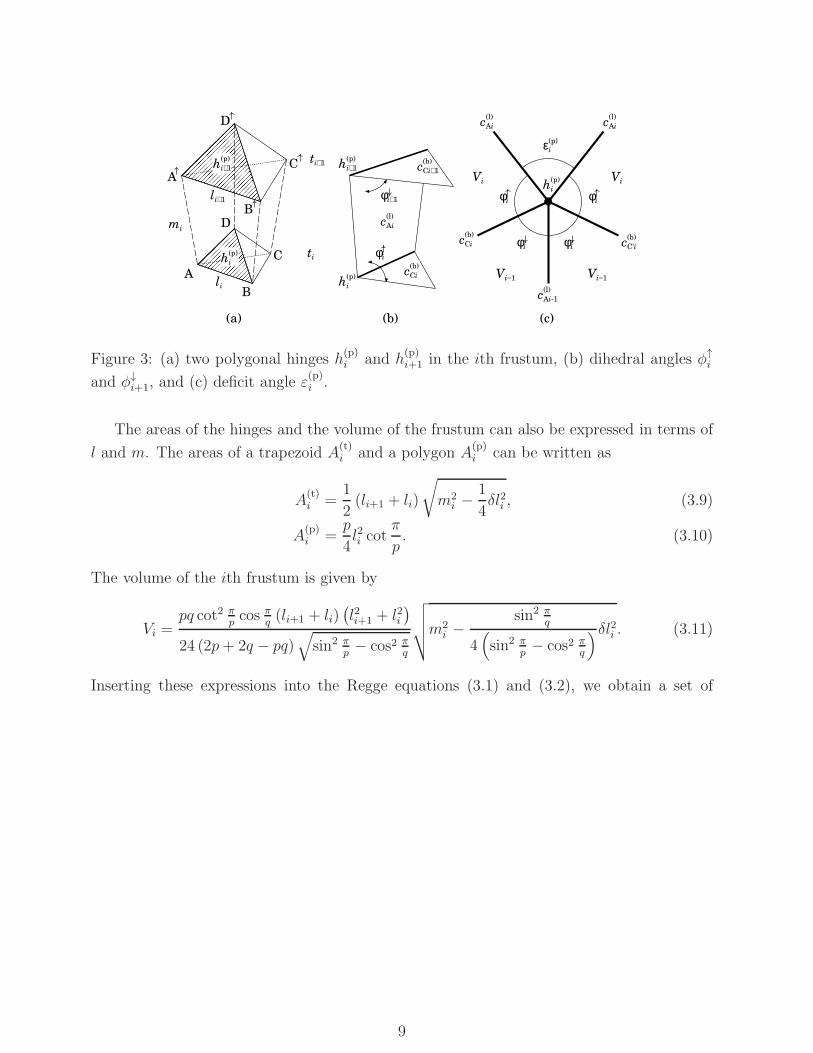
Figure 3: (a) two polygonal hinges h(p)i and h

(p)i+1 in the ith frustum, (b) dihedral angles φ↑

i

and φ↓i+1, and (c) deficit angle ε

(p)i .

The areas of the hinges and the volume of the frustum can also be expressed in terms of

l and m. The areas of a trapezoid A(t)i and a polygon A

(p)i can be written as

A(t)i =

1

2(li+1 + li)

√

m2i −

1

4δl2i , (3.9)

A(p)i =

p

4l2i cot

π

p. (3.10)

The volume of the ith frustum is given by

Vi =pq cot2 π

pcos π

q(li+1 + li)

(

l2i+1 + l2i)

24 (2p+ 2q − pq)√

sin2 πp− cos2 π

q

√

√

√

√m2i −

sin2 πq

4(

sin2 πp− cos2 π

q

)δl2i . (3.11)

Inserting these expressions into the Regge equations (3.1) and (3.2), we obtain a set of

9

recurrence relations:

ε(t)i

√

4m2i − δl2i

=rΛ

24

(

l2i+1 + l2i)

cot2 πpcos π

q√

4m2i

(

sin2 πp− cos2 π

q

)

− sin2 πqδl2i

, (3.12)

√

4m2i − δl2i ε

(t)i +

√

4m2i−1 − δl2i−1ε

(t)i−1

+l2i+1 − l2i

√

4m2i − δl2i

ε(t)i − l2i − l2i−1

√

4m2i−1 − δl2i−1

ε(t)i−1 + 2r cot

π

pliε

(p)i

=rΛ cot2 π

pcos π

q

24(

sin2 πp− cos2 π

q

)

[

(

l2i+1 + 2li+1li + 3l2i)

√

4m2i

(

sin2 π

p− cos2

π

q

)

− sin2 π

qδl2i

+(

3l2i + 2lili−1 + l2i−1

)

√

4m2i−1

(

sin2 π

p− cos2

π

q

)

− sin2 π

qδl2i−1

+

(

l4i+1 − l4i)

sin2 πq

√

4m2i

(

sin2 πp− cos2 π

q

)

− sin2 πqδl2i

−(

l4i − l4i−1

)

sin2 πq

√

4m2i−1

(

sin2 πp− cos2 π

q

)

− sin2 πqδl2i−1

]

.

(3.13)

These are non-linear recurrence relations for the edge and strut lengths li and mi. Evolution

of the polytopal universe can be investigated by taking the continuum time limit as in

Refs. [4, 8–10].

4 Continuum time limit

We are interested in the evolution of a model universe with a regular polytope as the Cauchy

surfaces. In continuum theory, Cauchy surfaces are defined as slices of space-time by constant

times. In the FLRW universe, the time axis is taken to be orthogonal to the Cauchy surfaces.

This seems to correspond to choosing the time axis to be orthogonal to the Cauchy cells.

One can identify the distance between the centers of circumspheres of the two Cauchy cells

in Fig. 1 with the Euclidean time interval δti = ti+1 − ti. This works for Cauchy cells of

regular polyhedrons [8, 9]. Later in this paper we consider Cauchy surfaces that are not

necessarily regular polytopes. For general polytopal substitutions for 3-spheres as Cauchy

surfaces, however, distances between two temporally consecutive Cauchy cells vary cell by

cell. One cannot identify the temporal distances with a common time interval δti, as noted

in Ref. [11] for polyhedral universe.

We avoid the subtleties in identifying the time coordinate by supposing a fictitious point

material in a state of rest spatially at each vertex of the polytopal Cauchy surface. Taking

ti as the proper time of a clock standing by the fictitious material particle, we can identify

10

strut length mi with the time interval

mi = δti. (4.1)

The time axis is not defined to be orthogonal to the polytopal Cauchy surfaces. The orthog-

onality of the temporal axis with the spatial ones is restored in the continuum limit. We

further choose all the time intervals δti to be equal and then take the continuum time limit

δti → dt. The edge lengths can be regarded as a smooth function of time li → l(t), and

δli =δliδtiδti → ldt, (4.2)

where l = dl/dt. It is straightforward to take the continuum time limit for Eqs. (3.12) and

(3.13). We find

ε(t)√

4− l2=rΛ

12

l2 cot2 πpcos π

q√

4(

sin2 πp− cos2 π

q

)

− l2 sin2 πq

, (4.3)

√

4− l2ε(t) +d

dt

(

ll√

4− l2ε(t)

)

+ 2rl cotπ

pφ↓

=rΛ

12

cot2 πpcos π

q

sin2 πp− cos2 π

q

[

3l2

√

4

(

sin2 π

p− cos2

π

q

)

− l2 sin2 π

q

+d

dt

l3l sin2 πq

√

4(

sin2 πp− cos2 π

q

)

− l2 sin2 πq

]

, (4.4)

where ε(t) and φ↓ are, respectively, the continuum time limits of Eqs. (3.5) and (3.7)

ε(t) = 2π − r arccos4(

sin2 πp− 2 cos2 π

q

)

+ l2 cos 2πq

4 sin2 πp− l2

, (4.5)

φ↓ =d

dtarccos

l cos πpcos π

q√

(

sin2 πp− cos2 π

q

)(

4 sin2 πp− l2

)

. (4.6)

Since we have fixed the strut lengths by Eq. (4.1), they disappear from the Regge equations.

Furthermore, substituting Eqs. (4.3) and (4.6) into the evolution equation (4.4), it can be

simplified as

l = −Λ

3l

(

1− l2

4 sin2 πp

)

1− 1

4l2 +

1

2

ll cos2 πp

4(

sin2 πp− cos2 π

q

)

− l2 sin2 πq

. (4.7)

11

One can easily verify that this is consistent with the Hamiltonian constraint (4.3). In other

words, the Hamiltonian constraint (4.3) can be obtained as the first integral of the evolution

equation (4.7) for the initial conditions

l (0) = l0 =

√

12

rΛ(2π − rθ0) cot

θ02tan

π

p, l (0) = 0, (4.8)

where θ0 = 2 arcsin [cos (π/q) / sin (π/p)] stands for a dihedral angle of the regular polyhedron

{p, q}. The cosmological constant must be positive for regular 4-polytopes as we see from

Eq. (4.8). This implies that the space-time is de Sitter-like. The 4-polytopal universe cannot

expand from or contract to a point but has minimum edge length l0, as does the continuum

solution, as we shall see below.

So far we have worked with piecewise linear space-time with Euclidean signature. To

argue the evolution of space-time we move to the Minkowskian signature by Wick rotation.

This can be done simply by letting l2, l → −l2,−l in Eqs. (4.3) and (4.7). We thus obtain

2π − r arccos4(

sin2 πp− 2 cos2 π

q

)

− l2 cos 2πq

4 sin2 πp+ l2

=rΛ

12l2

√

√

√

√

4 + l2

4(

sin2 πp− cos2 π

q

)

+ l2 sin2 πq

cot2π

pcos

π

q, (4.9)

l =Λ

3l

(

1 +l2

4 sin2 πp

)

1 +1

4l2 − 1

2

ll cos2 πp

4(

sin2 πp− cos2 π

q

)

+ l2 sin2 πq

. (4.10)

From the evolution equation (4.10) we see that the acceleration l is always positive. Hence the

polytopal universe, as the continuum solution, exhibits accelerated expansion or decelerated

contraction with the minimum edge length (4.8). The universe, however, reaches a maximum

size in a finite period of time as we shall see in the next section.

As a consistency check, let us consider the case of a vanishing cosmological constant

before turning to a detailed exposition of the behavior of the polytopal universe described

by the evolution equation (4.10). In the absence of a cosmological constant, the Hamiltonian

constraint (4.9) becomes

l2 =8(

sin2 πpsin2 π

r− cos2 π

q

)

cos 2πq+ cos 2π

r

= const. ≥ 0. (4.11)

There is no convex regular 4-polytope that has a Schlafli symbol satisfying this inequality.

In the case of l2 = 0, it admits {p, q, r} = {4, 3, 4} which gives a flat Cauchy surface

corresponding to the Minkowski metric. Moreover, in the case of l2 > 0, a Schlafli symbol

satisfying this inequality stands for a regular lattice of open Cauchy surface of constant

negative curvature. These results are consistent with solutions of the Friedmann equations

(see Table 1).

12

5 Numerical solution

In this section, we solve the Hamiltonian constraint (4.9) numerically and examine the

behaviors of the regular 4-polytopal universes. It is convenient to use the continuum time

limit of the dihedral angle (3.4). Let us denote it by θ:

θ = arccos4(

sin2 πp− 2 cos2 π

q

)

− l2 cos 2πq

4 sin2 πp+ l2

. (5.1)

Then l and l can be expressed as

l2 =4(

cos2 πq− sin2 π

psin2 θ

2

)

sin2 θ2− cos2 π

q

, (5.2)

l2 =12

rΛ(2π − rθ) tan2 π

pcot

θ

2. (5.3)

The first of these can be obtained directly from Eq. (5.1). The second can be derived from

the Hamiltonian constraint (4.9) by replacing l2 with Eq. (5.1). Since l2 ≥ 0, the dihedral

angle varies in the range θq ≤ θ ≤ θ0, where θq = (q − 2)π/q. The velocity l diverges for

θ = θq, while the edge length l approaches a finite value l = lp,q,r, where

lp,q,r =

√

12π

Λ

(

2

q+

2

r− 1

)

tanπ

qtan

π

p. (5.4)

This is contrasted with the polyhedral universe [11], where both l and l diverge at a finite

time.

To see these in more detail we eliminate the edge length from Eqs. (5.2) and (5.3) to

obtain

θ = ∓ 2 sin θ2csc θ0

2

2π − r (θ − sin θ)

√

√

√

√2rΛ

3(2π − rθ) sin θ

(

sin2 θ02− sin2 θq

2

)

(

sin2 θ02− sin2 θ

2

)

sin2 θ2− sin2 θq

2

. (5.5)

where the upper (lower) sign corresponds to an expanding (contracting) universe. Integrating

Eq. (5.5) numerically for the initial condition

θ (0) = θ0, (5.6)

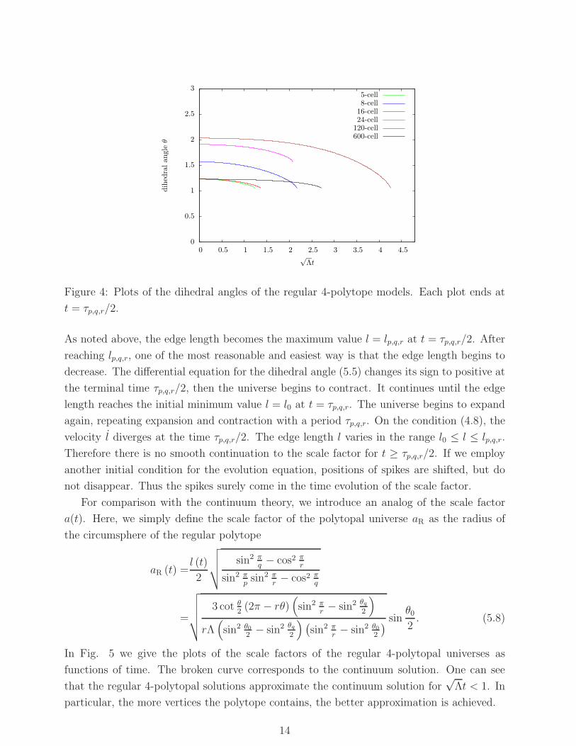
we obtain numerical solutions for the dihedral angle. In Fig. 4 we give the plots of dihedral

angles for the six types of regular 4-polytopes. They are monotone decreasing functions of

time for 0 ≤ t ≤ τp,q,r/2 and approach θq as t→ τp,q,r/2, where τp,q,r is defined by

τp,q,r = 2

∫ θ0

θq

dθ2π − r (θ − sin θ)

2 sin θ2csc θ0

2

√

√

√

√

√

3(

sin2 θ2− sin2 θq

2

)

2rΛ (2π − rθ)(

sin2 θ02− sin2 θq

2

)

(

sin2 θ02− sin2 θ

2

)

sin θ.

(5.7)

13

0

0.5

1

1.5

2

2.5

3

0 0.5 1 1.5 2 2.5 3 3.5 4 4.5

dihedralangleθ

√Λt

5-cell8-cell

16-cell24-cell120-cell600-cell

Figure 4: Plots of the dihedral angles of the regular 4-polytope models. Each plot ends at

t = τp,q,r/2.

As noted above, the edge length becomes the maximum value l = lp,q,r at t = τp,q,r/2. After

reaching lp,q,r, one of the most reasonable and easiest way is that the edge length begins to

decrease. The differential equation for the dihedral angle (5.5) changes its sign to positive at

the terminal time τp,q,r/2, then the universe begins to contract. It continues until the edge

length reaches the initial minimum value l = l0 at t = τp,q,r. The universe begins to expand

again, repeating expansion and contraction with a period τp,q,r. On the condition (4.8), the

velocity l diverges at the time τp,q,r/2. The edge length l varies in the range l0 ≤ l ≤ lp,q,r.

Therefore there is no smooth continuation to the scale factor for t ≥ τp,q,r/2. If we employ

another initial condition for the evolution equation, positions of spikes are shifted, but do

not disappear. Thus the spikes surely come in the time evolution of the scale factor.

For comparison with the continuum theory, we introduce an analog of the scale factor

a(t). Here, we simply define the scale factor of the polytopal universe aR as the radius of

the circumsphere of the regular polytope

aR (t) =l (t)

2

√

√

√

√

sin2 πq− cos2 π

r

sin2 πpsin2 π

r− cos2 π

q

=

√

√

√

√

√

3 cot θ2(2π − rθ)

(

sin2 πr− sin2 θq

2

)

rΛ(

sin2 θ02− sin2 θq

2

)

(

sin2 πr− sin2 θ0

2

)

sinθ02. (5.8)

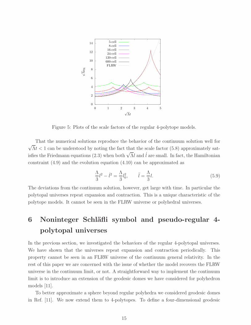
In Fig. 5 we give the plots of the scale factors of the regular 4-polytopal universes as

functions of time. The broken curve corresponds to the continuum solution. One can see

that the regular 4-polytopal solutions approximate the continuum solution for√Λt < 1. In

particular, the more vertices the polytope contains, the better approximation is achieved.

14

0

2

4

6

8

10

12

14

0 1 2 3 4 5

√ΛaR

√Λt

5-cell8-cell

16-cell24-cell120-cell600-cellFLRW

Figure 5: Plots of the scale factors of the regular 4-polytope models.

That the numerical solutions reproduce the behavior of the continuum solution well for√Λt < 1 can be understood by noting the fact that the scale factor (5.8) approximately sat-

isfies the Friedmann equations (2.3) when both√Λl and l are small. In fact, the Hamiltonian

constraint (4.9) and the evolution equation (4.10) can be approximated as

Λ

3l2 − l2 =

Λ

3l20, l =

Λ

3l. (5.9)

The deviations from the continuum solution, however, get large with time. In particular the

polytopal universes repeat expansion and contraction. This is a unique characteristic of the

polytope models. It cannot be seen in the FLRW universe or polyhedral universes.

6 Noninteger Schlafli symbol and pseudo-regular 4-

polytopal universes

In the previous section, we investigated the behaviors of the regular 4-polytopal universes.

We have shown that the universes repeat expansion and contraction periodically. This

property cannot be seen in an FLRW universe of the continuum general relativity. In the

rest of this paper we are concerned with the issue of whether the model recovers the FLRW

universe in the continuum limit, or not. A straightforward way to implement the continuum

limit is to introduce an extension of the geodesic domes we have considered for polyhedron

models [11].

To better approximate a sphere beyond regular polyhedra we considered geodesic domes

in Ref. [11]. We now extend them to 4-polytopes. To define a four-dimensional geodesic

15

Figure 6: Subdivision of a regular tetrahedron in the case of ν = 3.

dome, geodesic 4-dome in brief, we divide each cell of a regular polytope into smaller poly-

hedra. By projecting the vertices of the subdivided cells on to the circumsphere of the

original regular polytope we can define a geodesic 4-dome, a polytope having the points pro-

jected on to the circumsphere as the vertices. The method of subdivision is rather arbitrary

and depends on the regular polyhedron to be subdivided. In Ref. [7], Brewin proposed a

subdivision of a tetrahedron into tetrahedra that are not regular. Here we require that the

subdivision of a regular polyhedron should yield regular polyhedra of equal edge length. In

fact, a cube can be subdivided into ν3 smaller cubes of edge of a one-νth edge length, where

ν is a positive integer called “frequency”. Similarly, a regular tetrahedron and octahedron

can be subdivided into smaller regular tetrahedra and octahedra as illustrated in Fig. 6 for

a regular tetrahedron. We can then construct geodesic 4-domes by applying these subdivi-

sions to regular polytopes except for 120-cell. Since a dodecahedron has no subdivision into

smaller regular polyhedra, we will not consider geodesic 4-domes for 120-cell.

Regge calculus for the geodesic 4-domes becomes cumbersome as the frequency ν increases

as we have shown in Ref. [11] in three dimensions. We can avoid this by regarding the geodesic

4-domes as pseudo-regular 4-polytopes described by a non-integer Schlafli symbol. In what

follows we consider as the polytopal universe pseudo-regular 4-polytopes corresponding to

600-cell-based geodesic 4-domes. We first define the Schlafli symbol characterizing pseudo-

regular 4-polytopes.

For our purpose we summarize the numbers of cells, faces, edges, and vertices of the

geodesic 4-dome in Table 3. At a frequency ν each cell of a 600-cell can be subdivided

into ν(ν2 + 2)/3 tetrahedra and ν(ν2 − 1)/6 octahedra as depicted in Fig. 6. The geodesic

4-dome is then obtained by projecting the 600-cell tessellated by the 300(ν2 + 1) tiles on

16

Frequency ν

Tetrahedra 200ν (ν2 + 2)

N3 Octahedra 100ν (ν2 − 1)

Total 300ν (ν2 + 1)

Tetra-Tetra connectors 600ν (ν + 1)

N2 Octa-Octa connectors 600ν (ν − 1)

Tetra-Octa connectors 400ν (2ν2 − 3ν + 1)

Total 400ν (2ν2 + 1)

Five-way connectors 720ν

N1 Four-way connectors 600ν (ν2 − 1)

Total 120ν (5ν2 + 1)

N0 20ν (5ν2 + 1)

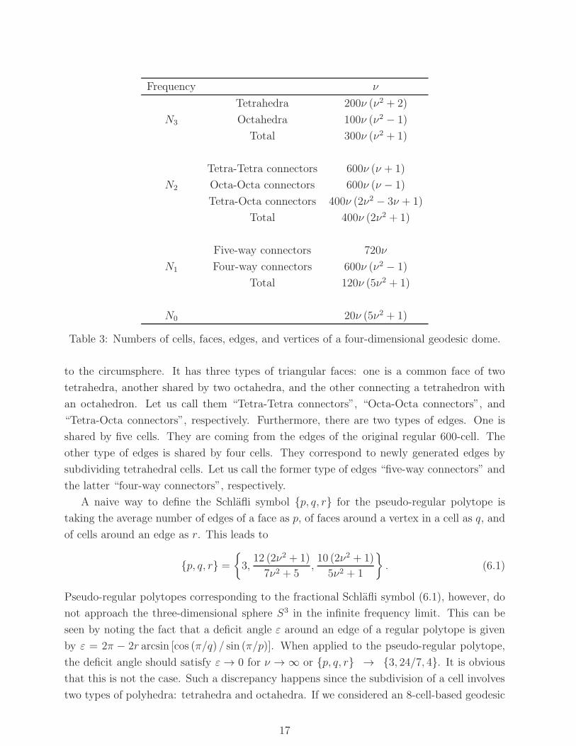
Table 3: Numbers of cells, faces, edges, and vertices of a four-dimensional geodesic dome.

to the circumsphere. It has three types of triangular faces: one is a common face of two

tetrahedra, another shared by two octahedra, and the other connecting a tetrahedron with

an octahedron. Let us call them “Tetra-Tetra connectors”, “Octa-Octa connectors”, and

“Tetra-Octa connectors”, respectively. Furthermore, there are two types of edges. One is

shared by five cells. They are coming from the edges of the original regular 600-cell. The

other type of edges is shared by four cells. They correspond to newly generated edges by

subdividing tetrahedral cells. Let us call the former type of edges “five-way connectors” and

the latter “four-way connectors”, respectively.

A naive way to define the Schlafli symbol {p, q, r} for the pseudo-regular polytope is

taking the average number of edges of a face as p, of faces around a vertex in a cell as q, and

of cells around an edge as r. This leads to

{p, q, r} =

{

3,12 (2ν2 + 1)

7ν2 + 5,10 (2ν2 + 1)

5ν2 + 1

}

. (6.1)

Pseudo-regular polytopes corresponding to the fractional Schlafli symbol (6.1), however, do

not approach the three-dimensional sphere S3 in the infinite frequency limit. This can be

seen by noting the fact that a deficit angle ε around an edge of a regular polytope is given

by ε = 2π − 2r arcsin [cos (π/q) / sin (π/p)]. When applied to the pseudo-regular polytope,

the deficit angle should satisfy ε → 0 for ν → ∞ or {p, q, r} → {3, 24/7, 4}. It is obviousthat this is not the case. Such a discrepancy happens since the subdivision of a cell involves

two types of polyhedra: tetrahedra and octahedra. If we considered an 8-cell-based geodesic

17

4-dome, we could obtain a pseudo-regular polytope characterized by a fractional Schlafli

symbol having a limit {p, q, r} → {4, 3, 4}.What we have shown is that the idea of averaging the Schlafli symbols does not work

except for an 8-cell-based geodesic 4-dome. We must employ another method of averaging

to define Schlafli symbols that not only have a smooth continuum limit but also preserve the

geometrical characteristics of polytopes.

To achieve this goal we introduce a set of angles ϑ2, ϑ3, and ϑ4, where ϑ2 is an interior

angle of a face of a regular polytope {p, q, r}, ϑ3 a dihedral angle of two adjacent faces, and

ϑ4 a hyperdihedral angle between two neighboring cells. They can be written in terms of p,

q, and r as

ϑ2 =p− 2

pπ = 2 arcsin

(

cosπ

p

)

, (6.2)

ϑ3 = 2 arcsin

(

cos πq

sin πp

)

, (6.3)

ϑ4 = 2 arcsin

sin πpcos π

r√

sin2 πp− cos2 π

q

. (6.4)

These can be solved with respect to the Schlafli symbol as

p(ϑ2) =π

arccos(

sin ϑ2

2

) , (6.5)

q(ϑ2, ϑ3) =π

arccos(

cos ϑ2

2sin ϑ3

2

) , (6.6)

r(ϑ3, ϑ4) =π

arccos(

cos ϑ3

2sin ϑ4

2

) . (6.7)

We are now able to extend the Schlafli symbol to an arbitrary pseudo-regular polytope

by substituting in Eqs. (6.5)–(6.7) the angles ϑ2,3,4 with averaged ones of tessellated parent

regular polytopes. With the help of Table 3, it is straightforward to obtain the averaged

angles of tessellated 600-cell as

ϑ2 =π

3, (6.8)

ϑ3 =(ν2 − 1)π + 3 arccos 1

3

2ν2 + 1, (6.9)

ϑ4 =(2ν2 − 3ν + 1)π + 3ν arccos

(

−3√5+18

)

2ν2 + 1. (6.10)

The pseudo-regular 4-polytope with the Schlafli symbol (Eqs. 6.5–6.10) has a smooth S3 limit

for ν → ∞ since {p, q, r} →{

3, π/ arccos(√

6/4)

, 4}

and, hence, the deficit angle around

an edge of a pseudo-regular 4-polytope satisfies ε = 2π−2r arcsin [cos (π/q) / sin (π/p)] → 0.

18

0

5

10

15

20

25

30

35

0 1 2 3 4 5 6 7 8

√ΛaR

√Λt

ν = 1ν = 2ν = 3ν = 4ν = 5

FLRW(ν = ∞)

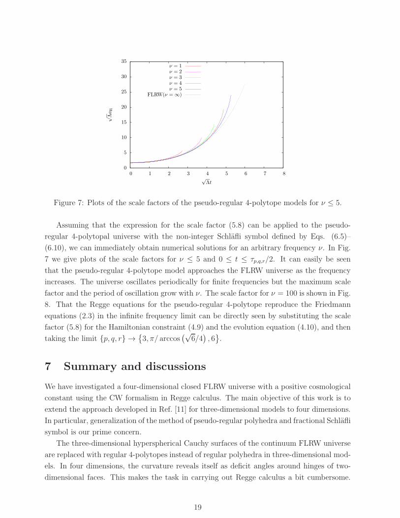
Figure 7: Plots of the scale factors of the pseudo-regular 4-polytope models for ν ≤ 5.

Assuming that the expression for the scale factor (5.8) can be applied to the pseudo-

regular 4-polytopal universe with the non-integer Schlafli symbol defined by Eqs. (6.5)–

(6.10), we can immediately obtain numerical solutions for an arbitrary frequency ν. In Fig.

7 we give plots of the scale factors for ν ≤ 5 and 0 ≤ t ≤ τp,q,r/2. It can easily be seen

that the pseudo-regular 4-polytope model approaches the FLRW universe as the frequency

increases. The universe oscillates periodically for finite frequencies but the maximum scale

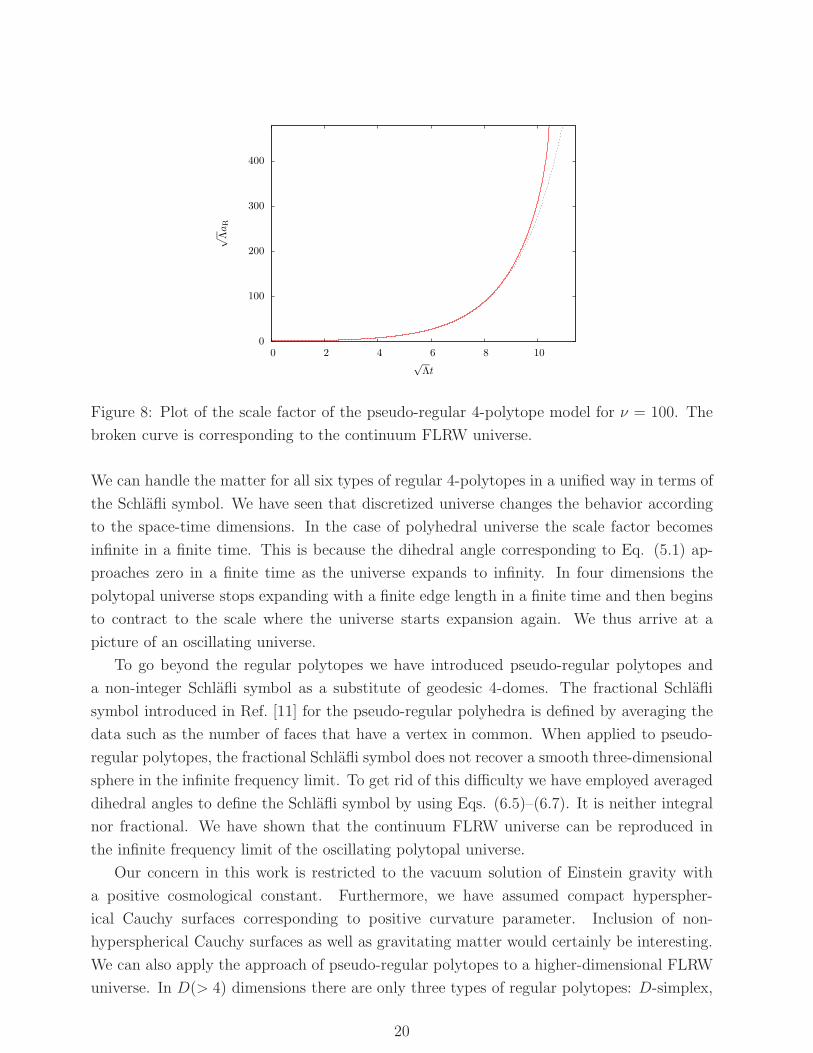
factor and the period of oscillation grow with ν. The scale factor for ν = 100 is shown in Fig.

8. That the Regge equations for the pseudo-regular 4-polytope reproduce the Friedmann

equations (2.3) in the infinite frequency limit can be directly seen by substituting the scale

factor (5.8) for the Hamiltonian constraint (4.9) and the evolution equation (4.10), and then

taking the limit {p, q, r} →{

3, π/ arccos(√

6/4)

, 6}

.

7 Summary and discussions

We have investigated a four-dimensional closed FLRW universe with a positive cosmological

constant using the CW formalism in Regge calculus. The main objective of this work is to

extend the approach developed in Ref. [11] for three-dimensional models to four dimensions.

In particular, generalization of the method of pseudo-regular polyhedra and fractional Schlafli

symbol is our prime concern.

The three-dimensional hyperspherical Cauchy surfaces of the continuum FLRW universe

are replaced with regular 4-polytopes instead of regular polyhedra in three-dimensional mod-

els. In four dimensions, the curvature reveals itself as deficit angles around hinges of two-

dimensional faces. This makes the task in carrying out Regge calculus a bit cumbersome.

19

0

100

200

300

400

0 2 4 6 8 10

√ΛaR

√Λt

Figure 8: Plot of the scale factor of the pseudo-regular 4-polytope model for ν = 100. The

broken curve is corresponding to the continuum FLRW universe.

We can handle the matter for all six types of regular 4-polytopes in a unified way in terms of

the Schlafli symbol. We have seen that discretized universe changes the behavior according

to the space-time dimensions. In the case of polyhedral universe the scale factor becomes

infinite in a finite time. This is because the dihedral angle corresponding to Eq. (5.1) ap-

proaches zero in a finite time as the universe expands to infinity. In four dimensions the

polytopal universe stops expanding with a finite edge length in a finite time and then begins

to contract to the scale where the universe starts expansion again. We thus arrive at a

picture of an oscillating universe.

To go beyond the regular polytopes we have introduced pseudo-regular polytopes and

a non-integer Schlafli symbol as a substitute of geodesic 4-domes. The fractional Schlafli

symbol introduced in Ref. [11] for the pseudo-regular polyhedra is defined by averaging the

data such as the number of faces that have a vertex in common. When applied to pseudo-

regular polytopes, the fractional Schlafli symbol does not recover a smooth three-dimensional

sphere in the infinite frequency limit. To get rid of this difficulty we have employed averaged

dihedral angles to define the Schlafli symbol by using Eqs. (6.5)–(6.7). It is neither integral

nor fractional. We have shown that the continuum FLRW universe can be reproduced in

the infinite frequency limit of the oscillating polytopal universe.

Our concern in this work is restricted to the vacuum solution of Einstein gravity with

a positive cosmological constant. Furthermore, we have assumed compact hyperspher-

ical Cauchy surfaces corresponding to positive curvature parameter. Inclusion of non-

hyperspherical Cauchy surfaces as well as gravitating matter would certainly be interesting.

We can also apply the approach of pseudo-regular polytopes to a higher-dimensional FLRW

universe. In D(> 4) dimensions there are only three types of regular polytopes: D-simplex,

20

D-cube, and D-orthoplex, as mentioned in Appendix A. We expect that this makes the

Regge calculus of polytopal universes in five or more dimensions easier.

Acknowledgments

The authors would like to thank Y. Hyakutake, N. Motoyui, M. Sakaguchi, and S. Tomizawa

for useful discussions.

A Circumradius of a regular D-polytope

For a regular 4-polytope {p, q, r}, the Schlafli symbol can be written in terms of dihedral

angles as Eqs. (6.5)–(6.7). For a regular D-polytope {p2, · · · , pD}, if we introduce ϑ0 = ϑ1 =

0 and denote by ϑi a dihedral angle of an i-dimensional face for i ≥ 2, we can express the

relation between Schlafli symbol and dihedral angles generally, as

pi =π

arccos(

cos ϑi−1

2sin ϑi

2

) . (A.1)

As can be seen from Eq. (A.1), the Schlafli symbol can be extended for i = 0, 1 as p0 = p1 = 2.

Then, a regularD-polytope can be associated with a set ofD+1 parameters {p0, p1, · · · , pD}.Let us denote half the length of a line segment by R1, and the radius of the circumsphere

of a D-polytope by RD. Using an extended Schlafli symbol {p0, p1, · · · , pD}, we can write

the first four of the circumradii as

R1 =l

2

√

√

√

√

sin2 πp1

sin2 πp0

, (A.2)

R2 =l

2

√

√

√

√

sin2 πp1

sin2 πp0sin2 π

p2

, (A.3)

R3 =l

2

√

√

√

√

sin2 πp1sin2 π

p3

sin2 πp0

(

sin2 πp2

− cos2 πp3

) , (A.4)

R4 =l

2

√

√

√

√

√

sin2 πp1

(

sin2 πp3

− cos2 πp4

)

sin2 πp0

(

sin2 πp2sin2 π

p4− cos2 π

p3

) , (A.5)

where l is the edge length of the regular polytopes.

From Eqs. (A.2)–(A.5), the recurrence relations for the circumradii can be guessed. In

21

Regular simplex Hypercube Orthoplex

{p2} {3} {4} {4}{p2, p3} {3, 3} {4, 3} {3, 4}{p2, p3, p4} {3, 3, 3} {4, 3, 3} {3, 3, 4}{p2, p3, · · · , pD−1, pD} {3, 3, · · · , 3, 3} {4, 3, · · · , 3, 3} {3, 3, · · · , 3, 4}RD

√

D2(D+1)

l√D2l

√22l

Table 4: The Schlafli symbols and the circumradii of regular simplices, hypercubes, and

orthoplices. l is an edge length of the polytopes.

the expression of Ri, letting

sin2 πpi−1

→ sin2 πpi−1

sin2 πpi+1

cos2 πpi−1

→ cos2 πpi−1

sin2 πpi+1

sin2 πpi−2

→ sin2 πpi−2

(

1− csc2 πpicos2 π

pi+1

)

cos2 πpi−2

→ cos2 πpi−2

(

1− csc2 πpicos2 π

pi+1

)

, (A.6)

then we obtain the expression of Ri+1. For the reader’s reference we give the next three

circumradii:

R5 =l2

√

sin2 πp1

(

sin2 πp3

sin2 πp5

−cos2 πp4

)

sin2 πp0

(

sin2 πp2

(

sin2 πp4

−cos2 πp5

)

−cos2 πp3

sin2 πp5

) , (A.7)

R6 =l2

√

sin2 πp1

(

sin2 πp3

(

sin2 πp5

−cos2 πp6

)

−cos2 πp4

sin2 πp6

)

sin2 πp0

(

sin2 πp2

(

sin2 πp4

sin2 πp6

−cos2 πp5

)

−cos2 πp3

(

sin2 πp5

−cos2 πp6

)) , (A.8)

R7 =l2

√

sin2 πp1

(

sin2 πp3

(

sin2 πp5

sin2 πp7

−cos2 πp6

)

−cos2 πp4

(

sin2 πp6

−cos2 πp7

))

sin2 πp0

(

sin2 πp2

(

sin2 πp4

(

sin2 πp6

−cos2 πp7

)

−cos2 πp5

sin2 πp7

)

−cos2 πp3

(

sin2 πp5

sin2 πp7

−cos2 πp6

)) . (A.9)

It is well known that in five or higher dimensions there are only three types of regular

polytopes: regular simplex, hypercube, and orthoplex. Hereafter we restrict our investiga-

tion to these regular polytopes. We summarize the Schlafli symbols and circumradii of the

polytopes in Table 4. As can be seen from this table, the circumradii are written as simple

functions in terms of dimension D. Therefore the recurrence relations (A.6) can easily be

inspected numerically. In fact, we have put it into practice and confirmed the correctness

for D ≤ 50.

As can also be seen from Table 4, D-simplex, D-cube, and D-orthoplex have the Schlafli

symbol p3 = · · · = pD−1 = 3 in common. Thus in five or higher dimensions a general

form of the circumradii of the D-polytopes might be given as a function of a set of three

parameters {D, p2, pD}. Substituting p0 = p1 = 2 and p3 = · · · = pD−1 = 3 into the functions

generated by the recurrence relations (A.6) and the initial condition (A.2), and comparing

22

On

On−1

On−3

On−1

2πpn

On−2

ϑn

ψn

ψn−1

χ

Figure 9: On is the circumcenter of Πn. On−1 and On−1 are the centers of two (n − 1)-

dimensional faces sharing Πn−2 centered at On−2, and On−3 is located at the center of Πn−3.

the expressions, we can guess the general form of the circumradius of a regular D-polytope;

RD =l

2

√

√

√

√

(D − 2) cos 2πpD

− 1

cos 2πp2

− D−32

cos(

2πp2

− 2πpD

)

− D−32

cos(

2πp2

+ 2πpD

)

+ cos 2πpD

(D = 5, 6, 7, · · · ) .

(A.10)

Assigning {p2, pD} = {3, 3} , {4, 3} , {3, 4} to Eq. (A.10), the circumradii of D-simplex,

D-cube, and D-orthoplex are reproduced, respectively.

Note added in proof

At the end of this paper, we give a short account of the relation between Schlafli symbol and

dihedral angles (A.1). We consider an arbitrary regular n-polytope {p0, p1, p2, · · · , pn} and

denote it by Πn , where p0 and p1 are introduced in Appendix A. Πn has regular (n − 1)-

polytopes {p0, p1, · · · , pn−1} as (n− 1)-dimensional faces. Similarly each k-dimensional face

Πk has regular polytopes Πk−1 for n ≥ k ≥ 1.

Let us choose a set of faces Π0,Π1, · · · ,Πn satisfying Π0 ⊂ Π1 ⊂ · · · ⊂ Πn and denote by

Ok the center of circumsphere of the Πk (n ≥ k ≥ 0). Furthermore we define the angles

ψn = ∠On−2OnOn−1, ψn−1 = ∠On−3On−1On−2, χ = ∠On−3OnOn−2. (A.11)

23

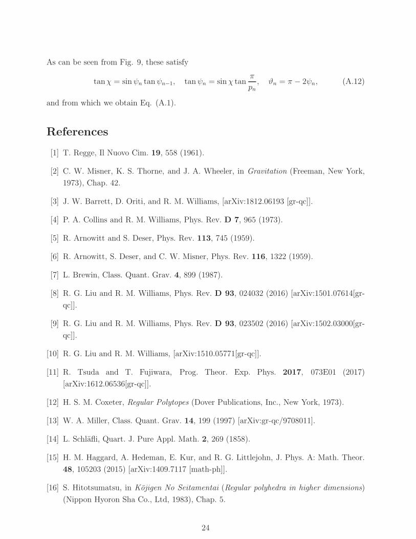
As can be seen from Fig. 9, these satisfy

tanχ = sinψn tanψn−1, tanψn = sinχ tanπ

pn, ϑn = π − 2ψn, (A.12)

and from which we obtain Eq. (A.1).

References

[1] T. Regge, Il Nuovo Cim. 19, 558 (1961).

[2] C. W. Misner, K. S. Thorne, and J. A. Wheeler, in Gravitation (Freeman, New York,

1973), Chap. 42.

[3] J. W. Barrett, D. Oriti, and R. M. Williams, [arXiv:1812.06193 [gr-qc]].

[4] P. A. Collins and R. M. Williams, Phys. Rev. D 7, 965 (1973).

[5] R. Arnowitt and S. Deser, Phys. Rev. 113, 745 (1959).

[6] R. Arnowitt, S. Deser, and C. W. Misner, Phys. Rev. 116, 1322 (1959).

[7] L. Brewin, Class. Quant. Grav. 4, 899 (1987).

[8] R. G. Liu and R. M. Williams, Phys. Rev. D 93, 024032 (2016) [arXiv:1501.07614[gr-

qc]].

[9] R. G. Liu and R. M. Williams, Phys. Rev. D 93, 023502 (2016) [arXiv:1502.03000[gr-

qc]].

[10] R. G. Liu and R. M. Williams, [arXiv:1510.05771[gr-qc]].

[11] R. Tsuda and T. Fujiwara, Prog. Theor. Exp. Phys. 2017, 073E01 (2017)

[arXiv:1612.06536[gr-qc]].

[12] H. S. M. Coxeter, Regular Polytopes (Dover Publications, Inc., New York, 1973).

[13] W. A. Miller, Class. Quant. Grav. 14, 199 (1997) [arXiv:gr-qc/9708011].

[14] L. Schlafli, Quart. J. Pure Appl. Math. 2, 269 (1858).

[15] H. M. Haggard, A. Hedeman, E. Kur, and R. G. Littlejohn, J. Phys. A: Math. Theor.

48, 105203 (2015) [arXiv:1409.7117 [math-ph]].

[16] S. Hitotsumatsu, in Kojigen No Seitamentai (Regular polyhedra in higher dimensions)

(Nippon Hyoron Sha Co., Ltd, 1983), Chap. 5.

24