students’ solutions manual partial differential ...students’ solutions manual partial...
TRANSCRIPT

Students’ Solutions Manual
PARTIAL DIFFERENTIAL
EQUATIONS
with FOURIER SERIES and
BOUNDARY VALUE PROBLEMS
Third Edition
NAKHLE H.ASMAR
University of Missouri
Contents
1 A Preview of Applications and Techniques 1
1.1 What Is a Partial Differential Equation? 1
1.2 Solving and Interpreting a Partial Differential Equation 3
2 Fourier Series 9
2.1 Periodic Functions 9
2.2 Fourier Series 15
2.3 Fourier Series of Functions with Arbitrary Periods 21
2.4 Half-Range Expansions: The Cosine and Sine Series 29
2.5 Mean Square Approximation and Parseval’s Identity 32
2.6 Complex Form of Fourier Series 36
2.7 Forced Oscillations 41
Supplement on Convergence
2.9 Uniform Convergence and Fourier Series 47
2.10 Dirichlet Test and Convergence of Fourier Series 48
3 Partial Differential Equations in Rectangular Coordinates 49
3.1 Partial Differential Equations in Physics and Engineering 49
3.3 Solution of the One Dimensional Wave Equation:
The Method of Separation of Variables 52
3.4 D’Alembert’s Method 60
3.5 The One Dimensional Heat Equation 69
3.6 Heat Conduction in Bars: Varying the Boundary Conditions 74
3.7 The Two Dimensional Wave and Heat Equations 87
3.8 Laplace’s Equation in Rectangular Coordinates 89
3.9 Poisson’s Equation: The Method of Eigenfunction Expansions 92
3.10 Neumann and Robin Conditions 94
Contents iii
4 Partial Differential Equations in
Polar and Cylindrical Coordinates 97
4.1 The Laplacian in Various Coordinate Systems 97
4.2 Vibrations of a Circular Membrane: Symmetric Case 99
4.3 Vibrations of a Circular Membrane: General Case 103
4.4 Laplace’s Equation in Circular Regions 108
4.5 Laplace’s Equation in a Cylinder 116
4.6 The Helmholtz and Poisson Equations 119
Supplement on Bessel Functions
4.7 Bessel’s Equation and Bessel Functions 124
4.8 Bessel Series Expansions 131
4.9 Integral Formulas and Asymptotics for Bessel Functions 141
5 Partial Differential Equations in Spherical Coordinates 142
5.1 Preview of Problems and Methods 142
5.2 Dirichlet Problems with Symmetry 144
5.3 Spherical Harmonics and the General Dirichlet Problem 147
5.4 The Helmholtz Equation with Applications to the Poisson, Heat,
and Wave Equations 153
Supplement on Legendre Functions
5.5 Legendre’s Differential Equation 156
5.6 Legendre Polynomials and Legendre Series Expansions 162
6 Sturm–Liouville Theory with Engineering Applications 167
6.1 Orthogonal Functions 167
6.2 Sturm–Liouville Theory 169
6.3 The Hanging Chain 172
6.4 Fourth Order Sturm–Liouville Theory 174
6.6 The Biharmonic Operator 176
6.7 Vibrations of Circular Plates 178
iv Contents
7 The Fourier Transform and Its Applications 179
7.1 The Fourier Integral Representation 179
7.2 The Fourier Transform 184
7.3 The Fourier Transform Method 193
7.4 The Heat Equation and Gauss’s Kernel 201
7.5 A Dirichlet Problem and the Poisson Integral Formula 210
7.6 The Fourier Cosine and Sine Transforms 213
7.7 Problems Involving Semi-Infinite Intervals 217
7.8 Generalized Functions 222
7.9 The Nonhomogeneous Heat Equation 233
7.10 Duhamel’s Principle 235
8 The Laplace and Hankel Transforms with Applications 238
8.1 The Laplace Transform 238
8.2 Further Properties of the Laplace transform 246
8.3 The Laplace Transform Method 258
8.4 The Hankel Transform with Applications 262
12 Green’s Functions and Conformal Mappings 268
12.1 Green’s Theorem and Identities 268
12.2 Harmonic Functions and Green’s Identities 272
12.3 Green’s Functions 274
12.4 Green’s Functions for the Disk and the Upper Half-Plane 276
12.5 Analytic Functions 277
12.6 Solving Dirichlet Problems with Conformal Mappings 286
12.7 Green’s Functions and Conformal Mappings 296
A Ordinary Differential Equations:
Review of Concepts and Methods A298
A.1 Linear Ordinary Differential Equations A298
A.2 Linear Ordinary Differential Equationswith Constant Coefficients A308
A.3 Linear Ordinary Differential Equations
with Nonconstant Coefficients A322
A.4 The Power Series Method, Part I A333
A.5 The Power Series Method, Part II A340
A.6 The Method of Frobenius A348
Section 1.1 What Is a Partial Differential Equation? 1
Solutions to Exercises 1.1
1. If u1 and u2 are solutions of (1), then
∂u1
∂t+∂u1
∂x= 0 and
∂u2
∂t+∂u2
∂x= 0.
Since taking derivatives is a linear operation, we have
∂
∂t(c1u1 + c2u2) +
∂
∂x(c1u1 + c2u2) = c1
∂u1
∂t+ c2
∂u2
∂t+ c1
∂u1
∂x+ c2
∂u2
∂x
= c1
=0︷ ︸︸ ︷(∂u1
∂t+∂u1
∂x
)+c2
=0︷ ︸︸ ︷(∂u2
∂t+ +
∂u2
∂x
)= 0,
showing that c1u1 + c2u2 is a solution of (1).3. (a) General solution of (1): u(x, t) = f(x− t). On the t-axis (x = 0): u(0, t) =t = f(0− t) = f(−t). Hence f(t) = −t and so u(x, t) = f(x− t) = −(x− t) = t−x.5. Let α = ax+ bt, β = cx+ dt, then
∂u
∂x=
∂u
∂α
∂α
∂x+∂u
∂β
∂β
∂x= a
∂u
∂α+ c
∂u
∂β
∂u
∂t=
∂u
∂α
∂α
∂t+∂u
∂β
∂β
∂t= b
∂u
∂α+ d
∂u
∂β.
Recalling the equation, we obtain
∂u
∂t− ∂u
∂x= 0 ⇒ (b− a)
∂u
∂α+ (d− c)
∂u
∂β= 0.
Let a = 1, b = 2, c = 1, d = 1. Then
∂u
∂α= 0 ⇒ u = f(β) ⇒ u(x, t) = f(x + t),
where f is an arbitrary differentiable function (of one variable).7. Let α = ax+ bt, β = cx+ dt, then
∂u
∂x=
∂u
∂α
∂α
∂x+∂u
∂β
∂β
∂x= a
∂u
∂α+ c
∂u
∂β
∂u
∂t=
∂u
∂α
∂α
∂t+∂u
∂β
∂β
∂t= b
∂u
∂α+ d
∂u
∂β.
The equation becomes
(b− 2a)∂u
∂α+ (d− 2c)
∂u
∂β= 2.
Let a = 1, b = 2, c = −1, d = 0. Then
2∂u
∂β= 2 ⇒ ∂u
∂β= 1.
Solving this ordinary differential equation in β, we get u = β + f(α) or u(x, t) =−x+ f(x + 2t).
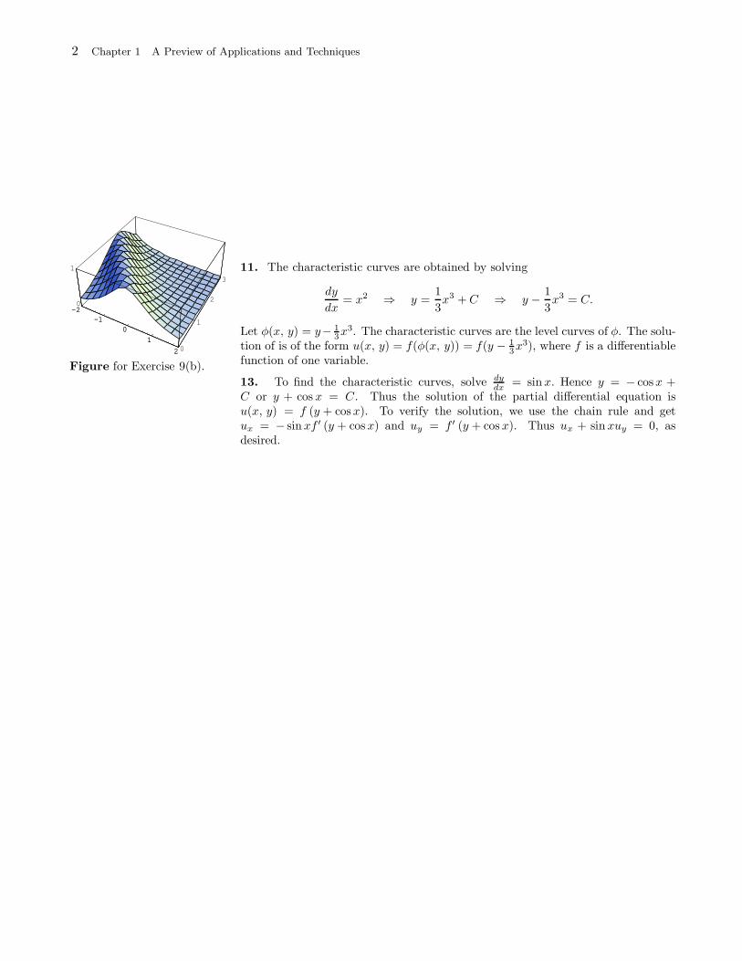
9. (a) The general solution in Exercise 5 is u(x, t) = f(x + t). When t = 0, we getu(x, 0) = f(x) = 1/(x2 + 1). Thus
u(x, t) = f(x + t) =1
(x+ t)2 + 1.
(c) As t increases, the wave f(x) = 11+x2 moves to the left.
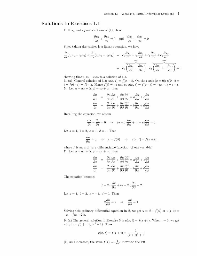
2 Chapter 1 A Preview of Applications and Techniques
-2
-1
0
1
2 0
1
2
3
0
1
-2
-1
0
1
2
Figure for Exercise 9(b).
11. The characteristic curves are obtained by solving
dy
dx= x2 ⇒ y =
1
3x3 +C ⇒ y − 1
3x3 = C.
Let φ(x, y) = y− 13x
3. The characteristic curves are the level curves of φ. The solu-tion of is of the form u(x, y) = f(φ(x, y)) = f(y − 1
3x3), where f is a differentiable
function of one variable.
13. To find the characteristic curves, solve dydx
= sinx. Hence y = − cosx +C or y + cos x = C. Thus the solution of the partial differential equation isu(x, y) = f (y + cosx). To verify the solution, we use the chain rule and getux = − sinxf ′ (y + cosx) and uy = f ′ (y + cos x). Thus ux + sinxuy = 0, asdesired.
Section 1.2 Solving and Interpreting a Partial Differential Equation 3
Exercises 1.2
1. We have
∂
∂t
(∂u
∂t
)= − ∂
∂t
(∂v
∂x
)and
∂
∂x
(∂v
∂t
)= − ∂
∂x
(∂u
∂x
).
So∂2u
∂t2= − ∂2v
∂t∂xand
∂2v
∂x∂t= −∂
2u
∂x2.
Assuming that ∂2v∂t∂x
= ∂2v∂x∂t
, it follows that ∂2u∂t2
= ∂2u∂x2 , which is the one dimensional
wave equation with c = 1. A similar argument shows that v is a solution of the onedimensional wave equation.3. uxx = F ′′(x+ ct) +G′′(x+ ct), utt = c2F ′′(x+ ct) + c2G(x− ct). So utt = cuxx,which is the wave equation.5. (a) We have u(x, t) = F (x + ct) + G(x− ct). To determine F and G, we usethe initial data:
u(x, 0) =1
1 + x2⇒ F (x) +G(x) =
1
1 + x2; (1)
∂u
∂t(x, 0) = 0 ⇒ cF ′(x) − cG′(x) = 0
⇒ F ′(x) = G′(x) ⇒ F (x) = G(x) +C, (2)
where C is an arbitrary constant. Plugging this into (1), we find
2G(x) +C =1
1 + x2⇒ G(x) =
1
2
[1
1 + x2−C
];
and from (2)
F (x) =1
2
[1
1 + x2+ C
].
Hence
u(x, t) = F (x+ ct) +G(x− ct) =1
2
[1
1 + (x+ ct)2+
1
1 + (x− ct)2
].
7. We have u(x, t) = F (x + ct) + G(x − ct). To determine F and G, we use theinitial data:
u(x, 0) = 0 ⇒ F (x) +G(x) = 0; (1)
∂u
∂t(x, 0) = −2xe−x2 ⇒ cF ′(x) − cG′(x) = −2xe−x2
⇒ cF (x)− cG(x) =
∫−2xe−x2
dx = e−x2
+C
⇒ F (x)−G(x) =e−x2
c+C, (2)
where we rewrote C/c as C to denote the arbitrary constant. Adding (2) and (1),we find
2F (x) =e−x2
c+C ⇒ F (x) =
1
2c
[e−x2
+ C];
and from (1)
G(x) = − 1
2c
[e−x2
+C].
Hence
u(x, t) = F (x+ ct) +G(x− ct) =1
2c
[e−(x+ct)2 − e−(x−ct)2
].
4 Chapter 1 A Preview of Applications and Techniques
8. We
9. As the hint suggests, we consider two separate problems: The problem inExercise 5 and the one in Exercise 7. Let u1(x, t) denote the solution in Exercise 5and u2(x, t) the solution in Exercise 7. It is straightforward to verify that u =u1 + u2 is the desired solution. Indeed, because of the linearity of derivatives, wehave utt = (u1)tt + (u2)tt = c2(u1)xx + c2(u2)xx, because u1 and u2 are solutionsof the wave equation. But c2(u1)xx + c2(u2)xx = c2(u1 + u2)xx = uxx and soutt = c2uxx, showing that u is a solution of the wave equation. Now u(x, 0) =u1(x, 0)+u2(x, 0) = 1/(1+x2)+0, because u1(x, 0) = 1/(1+x2) and u2(x, 0) = 0.
Similarly, ut(x, 0) = −2xe−x2
; thus u is the desired solution. The explicit formulafor u is
u(x, t) =1
2
[1
1 + (x+ ct)2+
1
1 + (x− ct)2
]+
1
2c
[e−(x+ct)2 − e−(x−ct)2
].
11. We have
∂2V
∂x2=
∂
∂x
(−L ∂I
∂t− RI
)= −L ∂2I
∂x∂t− R
∂I
∂x;
∂I
∂x= −C ∂V
∂t−GV ⇒ ∂V
∂t=
−1
C
[∂I
∂x+GV
];
so∂2V
∂t2=
−1
C
[∂2I
∂t∂x+G
∂V
∂t
].
To check that V verifies (1), we start with the right side
LC∂2V
∂t2+ (RC + LG)
∂V
∂t+RGV
= LC−1
C
[∂2I
∂t∂x+G
∂V
∂t
]+ (RC + LG)
−1
C
[∂I
∂x+GV
]+RGV
= −L ∂2I
∂t∂x−R
∂I
∂x− LG
C
=)︷ ︸︸ ︷[C∂V
∂t+∂I
∂x+GV
]
= −L ∂2I
∂t∂x−R
∂I
∂x=∂2V
∂x2,
which shows that V satisfies (1). To show that I satisfies (1), you can proceed as wedid for V or you can note that the equations that relate I and V are interchangedif we interchange L and C, and R and G. However, (1) remains unchanged if weinterchange L and C, and R and G. So I satisfies (1) if and only if V satisfies (1).
13. The function being graphed is
u(x, t) = sinπx cosπt− 1
2sin2πx cos 2πt +
1
3sin 3πx cos 3πt.
In frames 2, 4, 6, and 8, t = m4 , where m = 1, 3, 5, and 7. Plugging this into
u(x, t), we find
u(x, t) = sinπx cosmπ
4− 1
2sin 2πx cos
mπ
2+
1
3sin 3πx cos
3mπ
4.
For m = 1, 3, 5, and 7, the second term is 0, because cos mπ2 = 0. Hence at these
times, we have, for, m = 1, 3, 5, and 7,
u(x,m
4) = sinπx cosπt+
1
3sin 3πx cos 3πt.
Section 1.2 Solving and Interpreting a Partial Differential Equation 5
To say that the graph of this function is symmetric about x = 1/2 is equivalentto the assertion that, for 0 < x < 1/2, u(1/2 + x, m
4) = u(1/2 − x, m
4). Does this
equality hold? Let’s check:
u(1/2 + x,m
4) = sinπ(x+ 1/2) cos
mπ
4+
1
3sin3π(x+ 1/2) cos
3mπ
4
= cos πx cosmπ
4− 1
3cos 3πx cos
3mπ
4,
where we have used the identities sinπ(x + 1/2) = cos πx and sin 2π(x + 1/2) =− cos 3πx. Similalry,
u(1/2 − x,m
4) = sinπ(1/2 − x) cos
mπ
4+
1
3sin3π(1/2 − x) cos
3mπ
4
= cos πx cosmπ
4− 1
3cos 3πx cos
3mπ
4.
So u(1/2 + x, m4 ) = u(1/2− x, m
4 ), as expected.
15. Since the initial velocity is 0, from (10), we have
u(x, t) =
∞∑
n=1
bn sinnπx
Lcos
cnπt
L.
The initial condition u(x, 0) = f(x) = 12 sin πx
L + 14 sin 3πx
L implies that
∞∑
n=1
bn sinnπx
L= sin
2πx
L.
The equation is satisfied with the choice b1 = 0, b2 = 1, and all other bn’s are zero.This yields the solution
u(x, t) = sin2πx
Lcos
2cπt
L.
Note that the condition ut(x, 0) = 0 is also satisfied.
16. Since the initial velocity is 0, from (10), we have
u(x, t) =
∞∑
n=1
bn sinnπx
Lcos
cnπt
L.
The initial condition u(x, 0) = f(x) = 12 sin πx
L + 14 sin 3πx
L implies that
∞∑
n=1
bn sinnπx
L=
1
2sin
πx
L+
1
4sin
3πx
L.
Clearly, this equation is satisfied with the choice b1 = 12 , b3 = 1
4 , and all other bn’sare zero. This yields the solution
u(x, t) =1
2sin
πx
Lcos
cπt
L+
1
4sin
3πx
Lcos
3cπt
L.
Note that the condition ut(x, 0) = 0 is also satisfied.
17. Same reasoning as in the previous exercise, we find the solution
u(x, t) =1
2sin
πx
Lcos
cπt
L+
1
4sin
3πx
Lcos
3cπt
L+
2
5sin
7πx
Lcos
7cπt
L.
19. Reasoning as in the previous exercise, we satrt with the solution
u(x, t) =
∞∑
n=1
b∗n sinnπx
Lsin
cnπt
L.
6 Chapter 1 A Preview of Applications and Techniques
The initial condition u(x, 0) = 0 is clearly satisfied. To satisfy the second intialcondition, we must have
1
4sin
3πx
L− 1
10sin
6πx
L=
[∂
∂t
( ∞∑
n=1
b∗n sinnπx
Lsin
cnπt
L
)]
t=0
=
∞∑
n=1
cnπ
Lb∗n sin
nπx
L.
Thus
1
4=
3cπ
Lb∗3 ⇒ b∗3 =
L
12cπ;
− 1
10=
6cπ
Lb∗6 ⇒ b∗6 = − L
60cπ;
and all other b8n are 0. Thus
u(x, t) =L
12cπsin
3πx
Lsin
3cπt
L− L
60cπsin
6πx
Lsin
6cπt
L.
21. (a) We have to show that u(12 , t) is a constant for all t > 0. With c = L = 1,
we have
u(x, t) = sin 2πx cos 2πt ⇒ u(1/2, t) = sinπ cos 2πt = 0 for all t > 0.
(b) One way for x = 1/3 not to move is to have u(x, t) = sin 3πx cos 3πt. Thisis the solution that corresponds to the initial condition u(x, 0) = sin 3πx and∂u∂t (x, 0) = 0. For this solution, we also have that x = 2/3 does not move forall t.
22. (a) Reasoning as in Exercise 17, we find the solution to be
u(x, t) =1
2sin 2πx cos 2πt+
1
4sin 4πx cos 4πt.
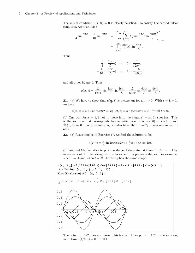
(b) We used Mathematica to plot the shape of the string at times t = 0 to t = 1 byincrements of .1. The string returns to some of its previous shapes. For example,when t = .1 and when t = .9, the string has the same shape.
u x_, t_ 1 2 Sin 2 Pi x Cos 2 Pi t 1 4 Sin 4 Pi x Cos 4 Pi t
tt Table u x, t , t, 0, 1, .1 ;
Plot Evaluate tt , x, 0, 1
1
2Cos 2 t Sin 2 x
1
4Cos 4 t Sin 4 x
0.2 0.4 0.6 0.8 1
-0.6
-0.4
-0.2
0.2
0.4
0.6
The point x = 1/2 does not move. This is clear: If we put x = 1/2 in the solution,we obtain u(1/2, t) = 0 for all t.
Section 1.2 Solving and Interpreting a Partial Differential Equation 7
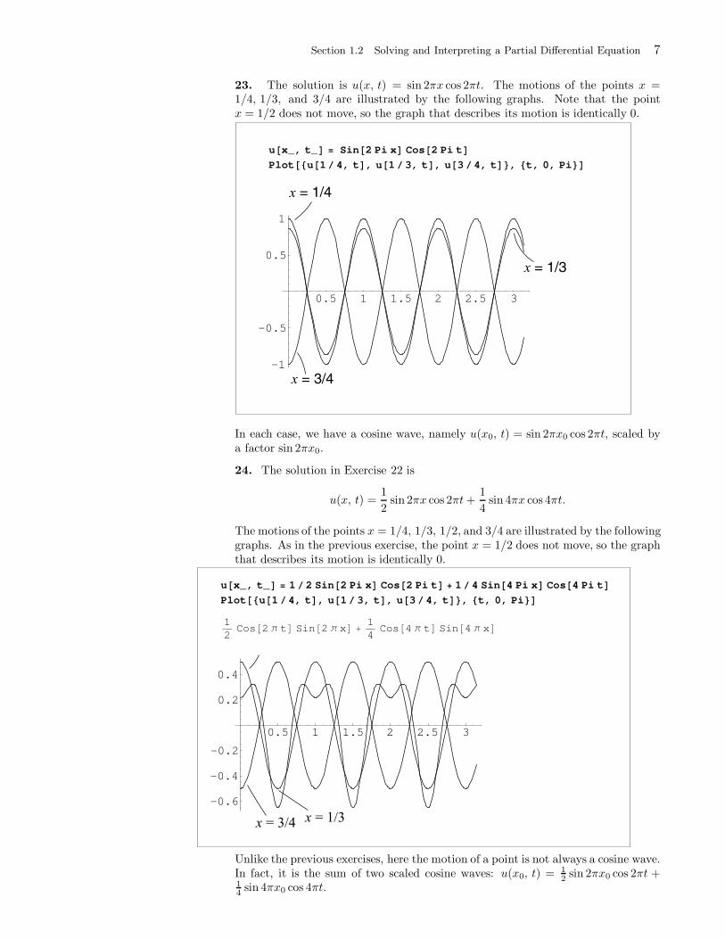
23. The solution is u(x, t) = sin 2πx cos 2πt. The motions of the points x =1/4, 1/3, and 3/4 are illustrated by the following graphs. Note that the pointx = 1/2 does not move, so the graph that describes its motion is identically 0.
u x_, t_ Sin 2 Pi x Cos 2 Pi t
Plot u 1 4, t , u 1 3, t , u 3 4, t , t, 0, Pi
0.5 1 1.5 2 2.5 3
-1
-0.5
0.5
1
= 1/4
= 3/4
= 1/3
In each case, we have a cosine wave, namely u(x0, t) = sin 2πx0 cos 2πt, scaled bya factor sin 2πx0.
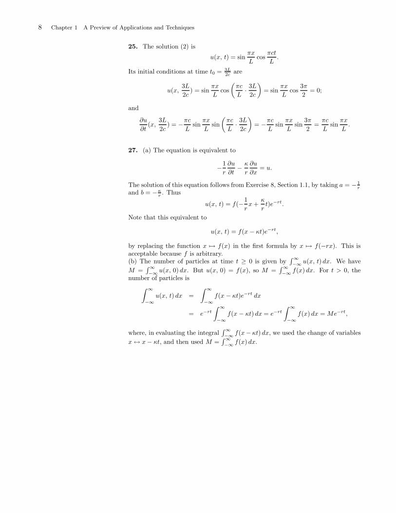
24. The solution in Exercise 22 is
u(x, t) =1
2sin 2πx cos 2πt+
1
4sin 4πx cos 4πt.
The motions of the points x = 1/4, 1/3, 1/2, and 3/4 are illustrated by the followinggraphs. As in the previous exercise, the point x = 1/2 does not move, so the graphthat describes its motion is identically 0.
u x_, t_ 1 2 Sin 2 Pi x Cos 2 Pi t 1 4 Sin 4 Pi x Cos 4 Pi t
Plot u 1 4, t , u 1 3, t , u 3 4, t , t, 0, Pi
1
2Cos 2 t Sin 2 x
1
4Cos 4 t Sin 4 x
0.5 1 1.5 2 2.5 3
-0.6
-0.4
-0.2
0.2
0.4
Unlike the previous exercises, here the motion of a point is not always a cosine wave.In fact, it is the sum of two scaled cosine waves: u(x0, t) = 1
2 sin 2πx0 cos 2πt +14
sin 4πx0 cos 4πt.
8 Chapter 1 A Preview of Applications and Techniques
25. The solution (2) is
u(x, t) = sinπx
Lcos
πct
L.
Its initial conditions at time t0 = 3L2c
are
u(x,3L
2c) = sin
πx
Lcos
(πc
L· 3L
2c
)= sin
πx
Lcos
3π
2= 0;
and
∂u
∂t(x,
3L
2c) = −πc
Lsin
πx
Lsin
(πc
L· 3L
2c
)= −πc
Lsin
πx
Lsin
3π
2=πc
Lsin
πx
L.
27. (a) The equation is equivalent to
−1
r
∂u
∂t− κ
r
∂u
∂x= u.
The solution of this equation follows from Exercise 8, Section 1.1, by taking a = −1r
and b = −κr. Thus
u(x, t) = f(−1
rx+
κ
rt)e−rt.
Note that this equivalent to
u(x, t) = f(x − κt)e−rt,
by replacing the function x 7→ f(x) in the first formula by x 7→ f(−rx). This isacceptable because f is arbitrary.(b) The number of particles at time t ≥ 0 is given by
∫∞−∞ u(x, t) dx. We have
M =∫∞−∞ u(x, 0) dx. But u(x, 0) = f(x), so M =
∫∞−∞ f(x) dx. For t > 0, the
number of particles is
∫ ∞
−∞u(x, t) dx =
∫ ∞
−∞f(x − κt)e−rt dx
= e−rt
∫ ∞
−∞f(x − κt) dx = e−rt
∫ ∞
−∞f(x) dx = Me−rt,
where, in evaluating the integral∫∞−∞ f(x− κt) dx, we used the change of variables
x↔ x− κt, and then used M =∫∞−∞ f(x) dx.
Section 2.1 Periodic Functions 9
Solutions to Exercises 2.11. (a) cosx has period 2π. (b) cos πx has period T = 2π
π = 2. (c) cos 23x has
period T = 2π2/3 = 3π. (d) cos x has period 2π, cos 2x has period π, 2π, 3π,.. A
common period of cosx and cos 2x is 2π. So cos x+ cos 2x has period 2π.
3. (a) The period is T = 1, so it suffices to describe f on an interval of length 1.From the graph, we have
f(x) =
0 if − 1
2 ≤ x < 0,1 if 0 ≤ x < 1
2 .
For all other x, we have f(x+ 1) = f(x).(b) f is continuous for all x 6= k
2 , where k is an integer. At the half-integers,
x = 2k+12 , using the graph, we see that limh→x+ f(h) = 0 and limh→x− f(h) =
1. At the integers, x = k, from the graph, we see that limh→x+ f(h) = 1 andlimh→x− f(h) = 0. The function is piecewise continuous.(c) Since the function is piecewise constant, we have that f ′(x) = 0 at all x 6= k
2 ,where k is an integer. It follows that f ′(x+) = 0 and f ′(x−) = 0 (Despite the factthat the derivative does not exist at these points; the left and right limits exist andare equal.)
5. This is the special case p = π of Exercise 6(b).
7. Suppose that Show that f1, f2, . . ., fn, . . . are T -periodic functions. Thismeans that fj(x + T ) = f(x) for all x and j = 1, 2, . . . , n. Let sn(x) = a1f1(x) +a2f2(x) + · · ·+ anfn(x). Then
sn(x+ T ) = = a1f1(x+ T ) + a2f2(x+ T ) + · · ·+ anfn(x+ T )
= a1f1(x) + a2f2(x) + · · ·+ anfn(x) = sn(x);
which means that sn is T -periodic. In general, if s(x) =∑∞
j=1 ajfj(x) is a seriesthat converges for all x, where each fj is T -periodic, then
s(x + T ) =
∞∑
j=1
ajfj(x+ T ) =
∞∑
j=1
ajfj(x) = s(x);
and so s(x) is T -periodic.
9. (a) Suppose that f and g are T -periodic. Then f(x+T ) · g(x+T ) = f(x) · g(x),and so f · g is T periodic. Similarly,
f(x+ T )
g(x+ T )=f(x)
g(x),
and so f/g is T periodic.(b) Suppose that f is T -periodic and let h(x) = f(x/a). Then
h(x+ aT ) = f
(x+ aT
a
)= f
(xa
+ T)
= f(xa
)(because f is T -periodic)
= h(x).
Thus h has period aT . Replacing a by 1/a, we find that the function f(ax) hasperiod T/a.(c) Suppose that f is T -periodic. Then g(f(x + T )) = g(f(x)), and so g(f(x)) isalso T -periodic.
11. Using Theorem 1,
∫ π/2
−π/2
f(x) dx =
∫ π
0
f(x) dx =
∫ π
0
sinx dx = 2.
10 Chapter 2 Fourier Series
13. ∫ π/2
−π/2
f(x) dx =
∫ π/2
0
1 dx = π/2.
15. Let F (x) =∫ x
af(t) dt. If F is 2π-periodic, then F (x) = F (x+ 2π). But
F (x+ 2π) =
∫ x+2π
a
f(t) dt =
∫ x
a
f(t) dt +
∫ x+2π
x
f(t) dt = F (x) +
∫ x+2π
x
f(t) dt.
Since F (x) = F (x+ 2π), we conclude that
∫ x+2π
x
f(t) dt = 0.
Applying Theorem 1, we find that∫ x+2π
x
f(t) dt =
∫ 2π
0
f(t) dt = 0.
The above steps are reversible. That is,∫ 2π
0
f(t) dt = 0 ⇒∫ x+2π
x
f(t) dt = 0
⇒∫ x
a
f(t) dt =
∫ x
a
f(t) dt+
∫ x+2π
x
f(t) dt =
∫ x+2π
a
f(t) dt
⇒ F (x) = F (x+ 2π);
and so F is 2π-periodic.
17. By Exercise 16, F is 2 periodic, because∫ 2
0f(t) dt = 0 (this is clear from
the graph of f). So it is enough to describe F on any interval of length 2. For0 < x < 2, we have
F (x) =
∫ x
0
(1 − t) dt = t− t2
2
∣∣∣x
0= x− x2
2.
For all other x, F (x+2) = F (x). (b) The graph of F over the interval [0, 2] consistsof the arch of a parabola looking down, with zeros at 0 and 2. Since F is 2-periodic,the graph is repeated over and over.
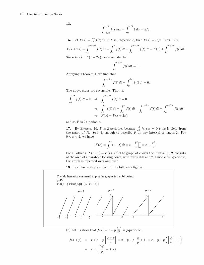
19. (a) The plots are shown in the following figures.
(b) Let us show that f(x) = x− p[
xp
]is p-periodic.
f(x+ p) = x+ p− p
[x+ p
p
]= x+ p− p
[x
p+ 1
]= x+ p− p
([x
p
]+ 1
)
= x− p
[x
p
]= f(x).
Section 2.1 Periodic Functions 11
From the graphs it is clear that f(x) = x for all 0 < x < p. To see this from theformula, use the fact that [t] = 0 if 0 ≤ t < 1. So, if 0 ≤ x < p, we have 0 ≤ x
p< 1,
so[
xp
]= 0, and hence f(x) = x.
20. (a) Plot of the function f(x) = x− 2p[
x+p2p
]for p = 1, 2, and π.
p 1
p
p 2
Plot x 2pFloor x p2 p , x, 2,2
(b)
f(x + 2p) = (x + 2p) − 2p
[(x+ 2p) + p
2p
]= (x+ 2p) − 2p
[x+ p
2p+ 1
]
= (x + 2p) − 2p
([x+ p
2p
]+ 1
)= x− 2p
[x+ p
2p
]= f(x).
So f is 2p-periodic. For −p < x < p, we have 0 < x+p2p < 1, hence
[x+p2p
]= 0, and
so f(x) = x− 2p[
x+p2p
]= x.
21. (a) With p = 1, the function f becomes f(x) = x−2[
x+12
], and its graph is the
first one in the group shown in Exercise 20. The function is 2-periodic and is equalto x on the interval −1 < x < 1. By Exercise 9(c), the function g(x) = h(f(x) is 2-periodic for any function h; in particular, taking h(x) = x2, we see that g(x) = f(x)2
is 2-periodic. (b) g(x) = x2 on the interval −1 < x < 1, because f(x) = x on that
interval. (c) Here is a graph of g(x) = f(x)2 =(x− 2
[x+12
])2, for all x.
Plot x 2 Floor x 1 2 ^2, x, 3, 3
-3 -2 -1 1 2 3
1
22. (a) As in Exercise 21, the function f(x) = x−2[
x+12
]is 2-periodic and is equal
to x on the interval −1 < x < 1. So, by Exercise 9(c), the function
g(x) = |f(x)| =
∣∣∣∣x− 2
[x+ 1
2
]∣∣∣∣
is 2-periodic and is clearly equal to |x| for all −1 < x < 1. Its graph is a triangularwave as shown in (b).
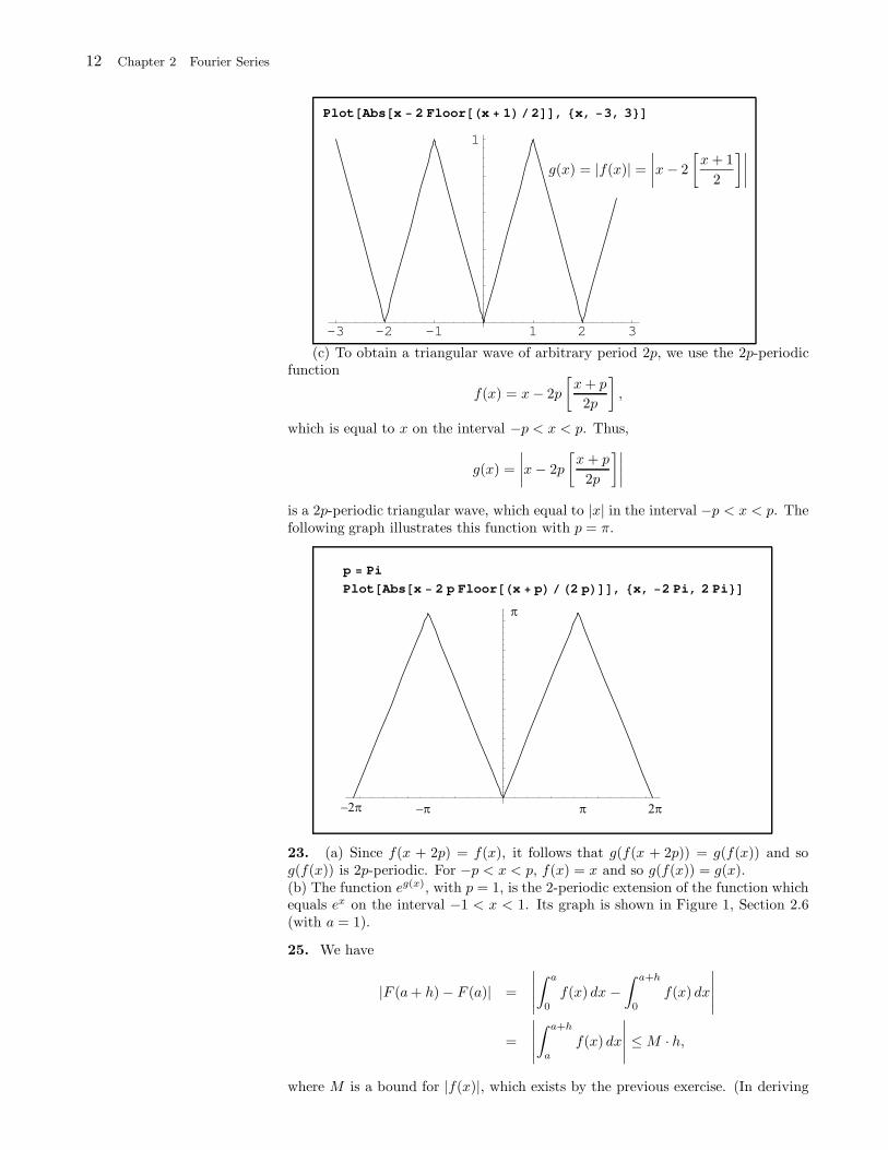
12 Chapter 2 Fourier Series
Plot Abs x 2 Floor x 1 2 , x, 3, 3
-3 -2 -1 1 2 3
1
(c) To obtain a triangular wave of arbitrary period 2p, we use the 2p-periodicfunction
f(x) = x− 2p
[x+ p
2p
],
which is equal to x on the interval −p < x < p. Thus,
g(x) =
∣∣∣∣x− 2p
[x+ p
2p
]∣∣∣∣
is a 2p-periodic triangular wave, which equal to |x| in the interval −p < x < p. Thefollowing graph illustrates this function with p = π.
p Pi
Plot Abs x 2 p Floor x p 2 p , x, 2 Pi, 2 Pi
23. (a) Since f(x + 2p) = f(x), it follows that g(f(x + 2p)) = g(f(x)) and sog(f(x)) is 2p-periodic. For −p < x < p, f(x) = x and so g(f(x)) = g(x).(b) The function eg(x), with p = 1, is the 2-periodic extension of the function whichequals ex on the interval −1 < x < 1. Its graph is shown in Figure 1, Section 2.6(with a = 1).
25. We have
|F (a+ h) − F (a)| =
∣∣∣∣∣
∫ a
0
f(x) dx −∫ a+h
0
f(x) dx
∣∣∣∣∣
=
∣∣∣∣∣
∫ a+h
a
f(x) dx
∣∣∣∣∣ ≤M · h,
where M is a bound for |f(x)|, which exists by the previous exercise. (In deriving
Section 2.1 Periodic Functions 13
the last inequality, we used the following property of integrals:
∣∣∣∣∣
∫ b
a
f(x) dx
∣∣∣∣∣ ≤ (b − a) ·M,
which is clear if you interpret the integral as an area.) As h → 0, M · h→ 0 and so|F (a+h)−F (a)| → 0, showing that F (a+h) → F (a), showing that F is continuousat a.(b) If f is continuous and F (a) =
∫ a
0f(x) dx, the fundamental theorem of calculus
implies that F ′(a) = f(a). If f is only piecewise continuous and a0 is a point ofcontinuity of f , let (xj−1, xj) denote the subinterval on which f is continuous anda0 is in (xj−1, xj). Recall that f = fj on that subinterval, where fj is a continuouscomponent of f . For a in (xj−1, xj), consider the functions F (a) =
∫ a
0 f(x) dx and
G(a) =∫ a
xj−1fj(x) dx. Note that F (a) = G(a) +
∫ xj−1
0f(x) dx = G(a) + c. Since
fj is continuous on (xj−1, xj), the fundamental theorem of calculus implies thatG′(a) = fj(a) = f(a). Hence F ′(a) = f(a), since F differs from G by a constant.
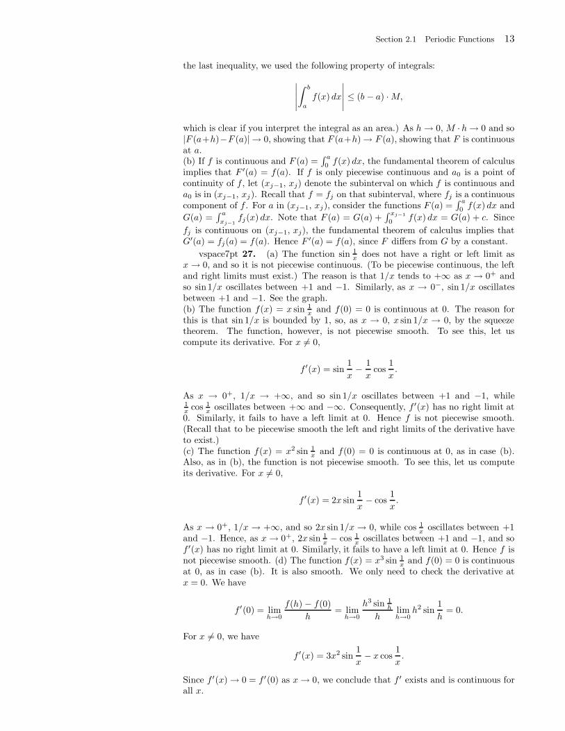
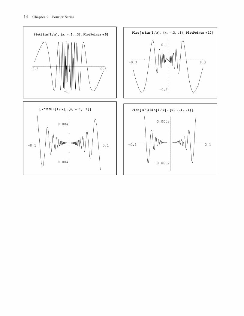
vspace7pt 27. (a) The function sin 1x does not have a right or left limit as
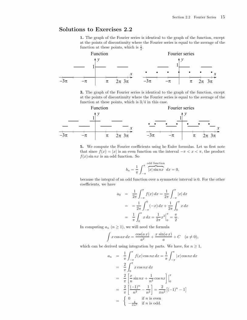
x → 0, and so it is not piecewise continuous. (To be piecewise continuous, the leftand right limits must exist.) The reason is that 1/x tends to +∞ as x → 0+ andso sin1/x oscillates between +1 and −1. Similarly, as x → 0−, sin 1/x oscillatesbetween +1 and −1. See the graph.(b) The function f(x) = x sin 1
x and f(0) = 0 is continuous at 0. The reason forthis is that sin 1/x is bounded by 1, so, as x → 0, x sin 1/x → 0, by the squeezetheorem. The function, however, is not piecewise smooth. To see this, let uscompute its derivative. For x 6= 0,
f ′(x) = sin1
x− 1
xcos
1
x.
As x → 0+, 1/x → +∞, and so sin 1/x oscillates between +1 and −1, while1x
cos 1x
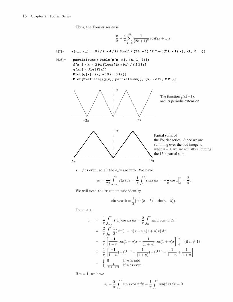
oscillates between +∞ and −∞. Consequently, f ′(x) has no right limit at0. Similarly, it fails to have a left limit at 0. Hence f is not piecewise smooth.(Recall that to be piecewise smooth the left and right limits of the derivative haveto exist.)(c) The function f(x) = x2 sin 1
x and f(0) = 0 is continuous at 0, as in case (b).Also, as in (b), the function is not piecewise smooth. To see this, let us computeits derivative. For x 6= 0,
f ′(x) = 2x sin1
x− cos
1
x.
As x → 0+, 1/x → +∞, and so 2x sin 1/x → 0, while cos 1x
oscillates between +1and −1. Hence, as x → 0+, 2x sin 1
x− cos 1
xoscillates between +1 and −1, and so
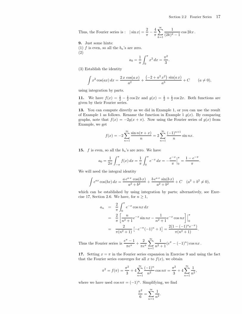
f ′(x) has no right limit at 0. Similarly, it fails to have a left limit at 0. Hence f isnot piecewise smooth. (d) The function f(x) = x3 sin 1
x and f(0) = 0 is continuousat 0, as in case (b). It is also smooth. We only need to check the derivative atx = 0. We have
f ′(0) = limh→0
f(h) − f(0)
h= lim
h→0
h3 sin 1h
hlimh→0
h2 sin1
h= 0.
For x 6= 0, we have
f ′(x) = 3x2 sin1
x− x cos
1
x.
Since f ′(x) → 0 = f ′(0) as x→ 0, we conclude that f ′ exists and is continuous forall x.
14 Chapter 2 Fourier Series
Plot Sin 1 x , x, .3, .3 , PlotPoints 5
-0.3 0.3
-1
1
Plot x Sin 1 x , x, .3, .3 , PlotPoints 10
-0.3 0.3
-0.2
0.1
x^2 Sin 1 x , x, .1, .1
-0.1 0.1
-0.004
0.004
Plot x^3 Sin 1 x , x, .1, .1
-0.1 0.1
-0.0002
0.0002
Section 2.2 Fourier Series 15
Solutions to Exercises 2.2
1. The graph of the Fourier series is identical to the graph of the function, exceptat the points of discontinuity where the Fourier series is equal to the average of thefunction at these points, which is 1
2.
3. The graph of the Fourier series is identical to the graph of the function, exceptat the points of discontinuity where the Fourier series is equal to the average of thefunction at these points, which is 3/4 in this case.
5. We compute the Fourier coefficients using he Euler formulas. Let us first notethat since f(x) = |x| is an even function on the interval −π < x < π, the productf(x) sin nx is an odd function. So
bn =1
π
∫ π
−π
odd function︷ ︸︸ ︷|x| sinnx dx = 0,
because the integral of an odd function over a symmetric interval is 0. For the othercoefficients, we have
a0 =1
2π
∫ π
−π
f(x) dx =1
2π
∫ π
−π
|x| dx
= =1
2π
∫ 0
−π
(−x) dx+1
2π
∫ π
0
x dx
=1
π
∫ π
0
x dx =1
2πx2∣∣∣π
0=π
2.
In computing an (n ≥ 1), we will need the formula∫x cos ax dx =
cos(a x)
a2+x sin(a x)
a+C (a 6= 0),
which can be derived using integration by parts. We have, for n ≥ 1,
an =1
π
∫ π
−π
f(x) cos nx dx =1
π
∫ π
−π
|x| cosnx dx
=2
π
∫ π
0
x cosnx dx
=2
π
[x
nsinnx+
1
n2cos nx
] ∣∣∣π
0
=2
π
[(−1)n
n2− 1
n2
]=
2
πn2
[(−1)n − 1
]
=
0 if n is even− 4
πn2 if n is odd.
16 Chapter 2 Fourier Series
Thus, the Fourier series is
π
2− 4
π
∞∑
k=0
1
(2k + 1)2cos(2k + 1)x .
s n_, x_ : Pi 2 4 Pi Sum 1 2 k 1 ^2 Cos 2 k 1 x , k, 0, n
partialsums Table s n, x , n, 1, 7 ;
f x_ x 2 Pi Floor x Pi 2 Pi
g x_ Abs f x
Plot g x , x, 3 Pi, 3 Pi
Plot Evaluate g x , partialsums , x, 2 Pi, 2 Pi
The function g(x) = | x |
and its periodic extension
Partial sums of
the Fourier series. Since we are
summing over the odd integers,
when n = 7, we are actually summing
the 15th partial sum.
7. f is even, so all the bn’s are zero. We have
a0 =1
2π
∫ π
−π
f(x) dx =1
π
∫ π
0
sinx dx = − 1
πcosx
∣∣∣π
0=
2
π.
We will need the trigonometric identity
sin a cos b =1
2
(sin(a − b) + sin(a+ b)
).
For n ≥ 1,
an =1
π
∫ π
−π
f(x) cos nx dx =2
π
∫ π
0
sinx cosnx dx
=2
π
∫ π
0
1
2
(sin(1 − n)x+ sin(1 + n)x
)dx
=1
π
[ −1
1 − ncos(1 − n)x− 1
(1 + n)cos(1 + n)x
] ∣∣∣π
0(if n 6= 1)
=1
π
[ −1
1 − n(−1)1−n − 1
(1 + n)(−1)1+n +
1
1 − n+
1
1 + n
]
=
0 if n is odd
4π(1−n2)
if n is even.
If n = 1, we have
a1 =2
π
∫ π
0
sinx cosx dx =1
π
∫ π
0
sin(2x) dx = 0.
Section 2.2 Fourier Series 17
Thus, the Fourier series is : | sinx| =2
π− 4
π
∞∑
k=1
1
(2k)2 − 1cos 2kx .
9. Just some hints:(1) f is even, so all the bn’s are zero.(2)
a0 =1
π
∫ π
0
x2 dx =π2
3.
(3) Establish the identity
∫x2 cos(ax) dx =
2 x cos(a x)
a2+
(−2 + a2 x2
)sin(a x)
a3+C (a 6= 0),
using integration by parts.
11. We have f(x) = 12 − 1
2 cos 2x and g(x) = 12 + 1
2 cos 2x. Both functions aregiven by their Fourier series.
13. You can compute directly as we did in Example 1, or you can use the resultof Example 1 as follows. Rename the function in Example 1 g(x). By comparinggraphs, note that f(x) = −2g(x + π). Now using the Fourier series of g(x) fromExample, we get
f(x) = −2∞∑
n=1
sinn(π + x)
n= 2
∞∑
n=1
(−1)n+1
nsinnx.
15. f is even, so all the bn’s are zero. We have
a0 =1
2π
∫ π
−π
f(x) dx =1
π
∫ π
0
e−x dx = −e−x
π
∣∣∣π
0=
1 − e−π
π.
We will need the integral identity
∫eax cos(bx) dx =
a ea x cos(b x)
a2 + b2+b ea x sin(b x)
a2 + b2+ C (a2 + b2 6= 0),
which can be established by using integration by parts; alternatively, see Exer-cise 17, Section 2.6. We have, for n ≥ 1,
an =2
π
∫ π
0
e−x cosnx dx
=2
π
[n
n2 + 1e−x sinnx− 1
n2 + 1e−x cos nx
] ∣∣∣π
0
=2
π(n2 + 1)
[−e−π(−1)n + 1
]=
2(1 − (−1)ne−π)
π(n2 + 1).
Thus the Fourier series iseπ − 1
πeπ+
2
πeπ
∞∑
n=1
1
n2 + 1(eπ − (−1)n) cosnx .
17. Setting x = π in the Fourier series expansion in Exercise 9 and using the factthat the Fourier series converges for all x to f(x), we obtain
π2 = f(π) =π2
3+ 4
∞∑
n=1
(−1)n
n2cos nπ =
π2
3+ 4
∞∑
n=1
1
n2,
where we have used cosnπ = (−1)n. Simplifying, we find
π2
6=
∞∑
n=1
1
n2.
18 Chapter 2 Fourier Series
19. (a) Let f(x) denote the function in Exercise 1 and w(x) the function inExample 5. Comparing these functions, we find that f(x) = 1
πw(x). Now using the
Fourier series of w, we find
f(x) =1
π
[π
2+ 2
∞∑
k=0
sin(2k + 1)x
2k + 1
]=
1
2+
2
π
∞∑
k=0
sin(2k + 1)x
2k + 1.
(b) Let g(x) denote the function in Exercise 2 and f(x) the function in (a). Com-paring these functions, we find that g(x) = 2f(x)− 1. Now using the Fourier seriesof f , we find
g(x) =4
π
∞∑
k=0
sin(2k + 1)x
2k + 1.
(c) Let k(x) denote the function in Figure 13, and let f(x) be as in (a). Comparingthese functions, we find that k(x) = f
(x + π
2
). Now using the Fourier series of f ,
we get
k(x) =1
2+
2
π
∞∑
k=0
sin(2k + 1)(x+ π2 )
2k + 1
=1
2+
2
π
∞∑
k=0
1
2k + 1
(sin[(2k+ 1)x]
=0︷ ︸︸ ︷cos[(2k+ 1)
π
2]+ cos[(2k + 1)x]
=(−1)k
︷ ︸︸ ︷sin[(2k + 1)
π
2])
=1
2+
2
π
∞∑
k=0
(−1)k
2k + 1cos[(2k+ 1)x].
(d) Let v(x) denote the function in Exercise 3, and let k(x) be as in (c). Comparingthese functions, we find that v(x) = 1
2
(k(x) + 1
). Now using the Fourier series of
k, we get
v(x) =3
4+
1
π
∞∑
k=0
(−1)k
2k + 1cos[(2k + 1)x].
21. (a) Interpreting the integral as an area (see Exercise 16), we have
a0 =1
2π· 1
2· π
2=
1
8.
To compute an, we first determine the equation of the function for π2 < x < π.
From Figure 16, we see that f(x) = 2π (π − x) if π
2 < x < π. Hence, for n ≥ 1,
an =1
π
∫ π
π/2
2
π
u︷ ︸︸ ︷(π − x)
v′
︷ ︸︸ ︷cosnx dx
=2
π2(π − x)
sinnx
n
∣∣∣π
π/2+
2
π2
∫ π
π/2
sinnx
ndx
=2
π2
[−π2n
sinnπ
2
]− 2
π2n2cosnx
∣∣∣π
π/2
= − 2
π2
[π
2nsin
nπ
2+
(−1)n
n2− 1
n2cos
nπ
2
].
Also,
bn =1
π
∫ π
π/2
2
π
u︷ ︸︸ ︷(π − x)
v′
︷ ︸︸ ︷sinnx dx
= − 2
π2(π − x)
cos nx
n
∣∣∣π
π/2− 2
π2
∫ π
π/2
cosnx
ndx
=2
π2
[π
2ncos
nπ
2+
1
n2sin
nπ
2
].
Section 2.2 Fourier Series 19
Thus the Fourier series representation of f is
f(x) =1
8+
2
π2
∞∑
n=1
−[π
2nsin
nπ
2+
(−1)n
n2− 1
n2cos
nπ
2
]cos nx
+
[π
2ncos
nπ
2+
1
n2sin
nπ
2
]sinnx
.
(b) Let g(x) = f(−x). By performing a change of variables x↔ −x in the Fourierseries of f , we obtain (see also Exercise 24 for related details) Thus the Fourierseries representation of f is
g(x) =1
8+
2
π2
∞∑
n=1
−[π
2nsin
nπ
2+
(−1)n
n2− 1
n2cos
nπ
2
]cosnx
−[π
2ncos
nπ
2+
1
n2sin
nπ
2
]sinnx
.
23. This exercise is straightforward and follows from the fact that the integral islinear.
25. For (a) and (b), see plots.
(c) We have sn(x) =∑n
k=1sin kx
k. So sn(0) = 0 and sn(2π) = 0 for all n. Also,
limx→0+ f(x) = π2 , so the difference between sn(x) and f(x) is equal to π/24 at
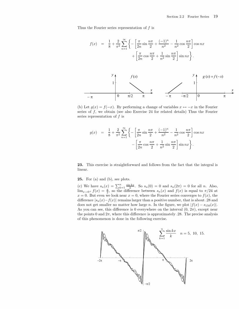
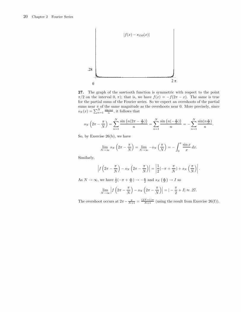
x = 0. But even we look near x = 0, where the Fourier series converges to f(x), thedifference |sn(x)−f(x)| remains larger than a positive number, that is about .28 anddoes not get smaller no matter how large n. In the figure, we plot |f(x)− s150(x)|.As you can see, this difference is 0 everywhere on the interval (0, 2π), except nearthe points 0 and 2π, where this difference is approximately .28. The precise analysisof this phenomenon is done in the following exercise.
20 Chapter 2 Fourier Series
27. The graph of the sawtooth function is symmetric with respect to the pointπ/2 on the interval 0, π); that is, we have f(x) = −f(2π − x). The same is truefor the partial sums of the Fourier series. So we expect an overshoots of the partialsums near π of the same magnitude as the overshoots near 0. More precisely, sincesN (x) =
∑Nn=1
sin nxn , it follows that
sN
(2π − π
N
)=
N∑
n=1
sin(n(2π − π
N ))
n=
N∑
n=1
sin(n(− π
N ))
n= −
N∑
n=1
sin(n πN )
n.
So, by Exercise 26(b), we have
limN→∞
sN
(2π − π
N
)= lim
N→∞−sN
( πN
)= −
∫ π
0
sinx
xdx.
Similarly,
∣∣∣f(2π − π
N
)− sN
(2π − π
N
)∣∣∣ =
∣∣∣∣1
2(−π +
π
N) + sN
( πN
)∣∣∣∣ .
As N → ∞, we have 12(−π + π
N) → −π
2and sN
(πN
)→ I so
limN→∞
∣∣∣f(2π − π
N
)− sN
(2π − π
N
)∣∣∣ = | − π
2+ I| ≈ .27.
The overshoot occurs at 2π− πN+1 = (2N+1)π
N+1 (using the result from Exercise 26(f)).
Section 2.3 Fourier Series of Functions with Arbitrary Periods 21
Solutions to Exercises 2.31. (a) and (b) Since f is odd, all the an’s are zero and
bn =2
p
∫ p
0
sinnπ
pdx
=−2
nπcos
nπ
p
∣∣∣π
0=
−2
nπ
[(−1)n − 1
]
=
0 if n is even,4
nπif n is odd.
Thus the Fourier series is4
π
∞∑
k=0
1
(2k + 1)sin
(2k + 1)π
px. At the points of discon-
tinuity, the Fourier series converges to the average value of the function. In thiscase, the average value is 0 (as can be seen from the graph.
3. (a) and (b) The function is even so all the bn’s are zero,
a0 =1
p
∫ p
0
a[(1 − (
x
p)2]dx =
a
p(x− 1
3p2x3)∣∣∣p
0=
2
3a;
and with the help of the integral formula from Exercise 9, Section 2.2, for n ≥ 1,
an =2a
p
∫ p
0
(1 − x2
p2) cos
nπx
pdx = −2a
p3
∫ p
0
x2 cosnπx
pdx
= −2a
p3
[2x
p2
(nπ)2cos
nπx
p+
p3
(nπ)3(−2 +
(nπ)2
p2)x2 sin
nπx
p
] ∣∣∣p
0
= −4a(−1)n
n2π2.
Thus the Fourier series is2
3a + 4a
∞∑
n=1
(−1)n+1
(nπ)2cos(
nπ
px). Note that the function
is continuous for all x.
5. (a) and (b) The function is even. It is also continuous for all x. All the bns are0. Also, by computing the area between the graph of f and the x-axis, from x = 0to x = p, we see that a0 = 0. Now, using integration by parts, we obtain
an =2
p
∫ p
0
−(
2c
p
)(x− p/2) cos
nπ
px dx = −4c
p2
∫ p
0
u︷ ︸︸ ︷(x− p/2)
v′
︷ ︸︸ ︷cos
nπ
px dx
= −4c
p2
=0︷ ︸︸ ︷p
nπ(x− p/2) sin
nπ
px∣∣∣p
x=0− p
nπ
∫ p
0
sinnπ
px dx
= −4c
p2
p2
n2π2cos
nπ
px∣∣∣p
x=0=
4c
n2π2(1 − cosnπ)
=
0 if n is even,
8cn2π2 if n is odd.
Thus the Fourier series is
f(x) =8c
π2
∞∑
k=0
cos[(2k + 1)π
px]
(2k + 1)2.
7. The function in this exercise is similar to the one in Example 3. Start with theFourier series in Example 3, multiply it by 1/c, then change 2p ↔ p (this is not a
22 Chapter 2 Fourier Series
change of variables, we are merely changing the notation for the period from 2p top) and you will get the desired Fourier series
f(x) =2
π
∞∑
n=1
sin(
2nπxp
)
n.
The function is odd and has discontinuities at x = ±p + 2kp. At these points, theFourier series converges to 0.
9. The function is even; so all the bn’s are 0,
a0 =1
p
∫ p
0
e−cx dx = − 1
cpe−cx
∣∣∣p
0=
1 − e−cp
cp;
and with the help of the integral formula from Exercise 15, Section 2.2, for n ≥ 1,
an =2
p
∫ p
0
e−cx cosnπx
pdx
=2
p
1
n2π2 + p2c2
[nπpe−cx sin
nπx
p− p2ce−cx cos
nπx
p
] ∣∣∣p
0
=2pc
n2π2 + p2c2[1 − (−1)ne−cp
].
Thus the Fourier series is
1
pc(1 − e−cp) + 2cp
∞∑
n=1
1
c2p2 + (nπ)2(1 − e−cp(−1)n) cos(
nπ
px) .
11. We note that the function f(x) = x sinx (−π < x < π) is the product of sinxwith a familiar function, namely, the 2π-periodic extension of x (−π < x < π). Wecan compute the Fourier coefficients of f(x) directly or we can try to relate themto the Fourier coefficients of g(x) = x. In fact, we have the following useful fact.
Suppose that g(x) is an odd function and write its Fourier series representation
as
g(x) =
∞∑
n=1
bn sinnx,
where bn is the nth Fourier coefficient of g. Let f(x) = g(x) sinx. Then f is even
and its nth cosine Fourier coefficients, an, are given by
a0 =b12, a1 =
b22, an =
1
2[bn+1 − bn−1] (n ≥ 2).
To prove this result, proceed as follows:
f(x) = sinx∞∑
n=1
bn sinnx
=
∞∑
n=1
bn sinx sinnx
=
∞∑
n=1
bn2
[− cos[(n+ 1)x] + cos[(n− 1)x]
].
To write this series in a standard Fourier series form, we reindex the terms, as
Section 2.3 Fourier Series of Functions with Arbitrary Periods 23
follows:
f(x) =
∞∑
n=1
(−bn
2cos[(n+ 1)x]
)+
∞∑
n=1
(bn2
cos[(n− 1)x]
)
=
∞∑
n=2
(−bn−1
2cos nx
)+
∞∑
n=0
(bn+1
2cos nx
)
=
∞∑
n=2
(−bn−1
2cos nx
)b12
+b22
cos x+
∞∑
n=2
(bn+1
2cosnx
)
=b12
+b22
cosx+∞∑
n=2
(bn+1
2− bn−1
2
)cos nx.
This proves the desired result. To use this result, we recall the Fourier series from
Exercise 2: For −π < x < π, g(x) = x = 2∑∞
n=1(−1)n+1
n sinnx; so b1 = 2,
b2 = −1/2 and bn = 2(−1)n+1
n for n ≥ 2. So, f(x) = x sinx =∑∞
n=1 an cosnx,where a0 = 1, a1 = −1/2, and, for n ≥ 2,
an =1
2
[2(−1)n+2
n+ 1− 2(−1)n
n− 1
]=
2(−1)n+1
n2 − 1.
Thus, for −π < x < π,
x sinx = 1 − cosx
2+ 2
∞∑
n=2
2(−1)n+1
n2 − 1cos nx.
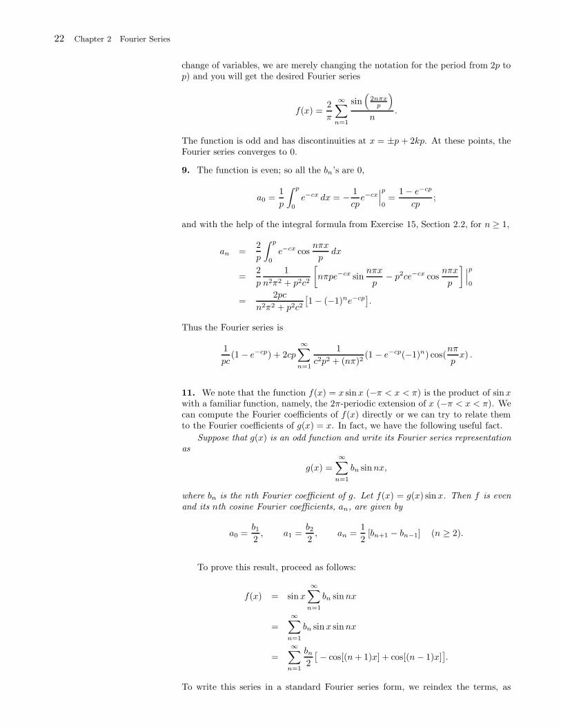
The convergence of the Fourier series is illustrated in the figure. Note that thepartial sums converge uniformly on the entire real line. This is a consequenceof the fact that the function is piecewise smooth and continuous for all x. Thefollowing is the 8th partial sum.
s n_, x_ 1 Cos x 2 2 Sum 1 ^ k 1 k^2 1 Cos k x , k, 2, n ;
Plot Evaluate x Sin x , s 8, x , x, Pi, Pi
1.75
To plot the function over more than one period, we can use the Floor functionto extend it outside the interval (−π, π). In what follows, we plot the function andthe 18th partial sum of its Fourier series. The two graphs are hard to distinguishfrom one another.
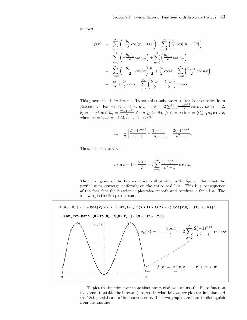
24 Chapter 2 Fourier Series
f x_ x Sin x ;
g x_ x 2 Pi Floor x Pi 2 Pi ;
h x_ f g x ;
Plot Evaluate h x , s 18, x , x, 2 Pi, 2 Pi
1.75
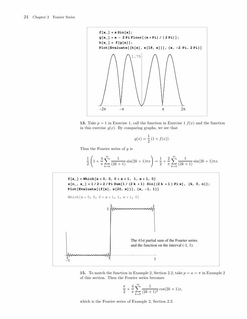
13. Take p = 1 in Exercise 1, call the function in Exercise 1 f(x) and the functionin this exercise g(x). By comparing graphs, we see that
g(x) =1
2(1 + f(x)) .
Thus the Fourier series of g is
1
2
(1 +
4
π
∞∑
k=0
1
(2k + 1)sin(2k + 1)πx
)=
1
2+
2
π
∞∑
k=0
1
(2k + 1)sin(2k + 1)πx.
f x_ Which x 0, 0, 0 x 1, 1, x 1, 0
s n_, x_ 1 2 2 Pi Sum 1 2 k 1 Sin 2 k 1 Pi x , k, 0, n ;
Plot Evaluate f x , s 20, x , x, 1, 1
Which x 0, 0, 0 x 1, 1, x 1, 0
The 41st partial sum of the Fourier series
and the function on the interval (-1, 1).
15. To match the function in Example 2, Section 2.2, take p = a = π in Example 2of this section. Then the Fourier series becomes
π
2+
4
π
∞∑
k=0
1
(2k + 1)2cos(2k + 1)x,
which is the Fourier series of Example 2, Section 2.2.
Section 2.3 Fourier Series of Functions with Arbitrary Periods 25
17. (a) Take x = 0 in the Fourier series of Exercise 4 and get
0 =p2
3− 4p2
π2
∞∑
n=1
(−1)n−1
n2⇒ π2
12=
∞∑
n=1
(−1)n−1
n2.
(b) Take x = p in the Fourier series of Exercise 4 and get
p2 =p2
3− 4p2
π2
∞∑
n=1
(−1)n−1(−1)n
n2⇒ π2
6=
∞∑
n=1
1
n2.
Summing over the even and odd integers separately, we get
π2
6=
∞∑
n=1
1
n2=
∞∑
k=0
1
(2k + 1)2+
∞∑
k=1
1
(2k)2.
But∑∞
k=11
(2k)2= 1
4
∑∞k=1
1k2 = 1
4π2
6. So
π2
6=
∞∑
k=0
1
(2k + 1)2+π2
24⇒
∞∑
k=0
1
(2k + 1)2=π2
6− π2
24=π2
8.
19. This is very similar to the proof of Theorem 2(i). If f(x) =∑∞
n=1 bn sin nπpx,
then, for all x,
f(−x) =
∞∑
n=1
bn sin(−nπpx) = −
∞∑
n=1
bn sinnπ
px = −f(x),
and so f is odd. Conversely, suppose that f is odd. Then f(x) cos nπpx is odd and,
from (10), we have an = 0 for all n. Use (5), (9), and the fact that f(x) sin nπp x is
even to get the formulas for the coefficients in (ii).23. From the graph, we have
f(x) =
−2x− 1 if − 1 < x < 0,1 if 0 < x < 1.
So
f(−x) =
1 if − 1 < x < 0,−1 + 2x if 0 < x < 1;
hence
fe(x) =f(x) + f(−x)
2=
−x if − 1 < x < 0,x if 0 < x < 1,
and
fo(x) =f(x) − f(−x)
2=
−x− 1 if − 1 < x < 0,1 − x if 0 < x < 1,
As expected, f(x) = fe(x)+fo(x). Note that, fe(x) = |x| for −1 < x < 1. Let g(x)be the function in Example 2 with p = 1. Then fe(x) = g(x). So from Example 1with p = 1, we obtain
fe(x) =1
2− 4
π2
∞∑
k=0
1
(2k + 1)2cos[(2k + 1)πx].
Note that fo(x) = 1 − x for 0 < x < 2. The Fourier series of fo follows fromExercise 7 with p = 2. Thus
fo(x) =2
π
∞∑
n=1
sin(nπx)
n.
26 Chapter 2 Fourier Series
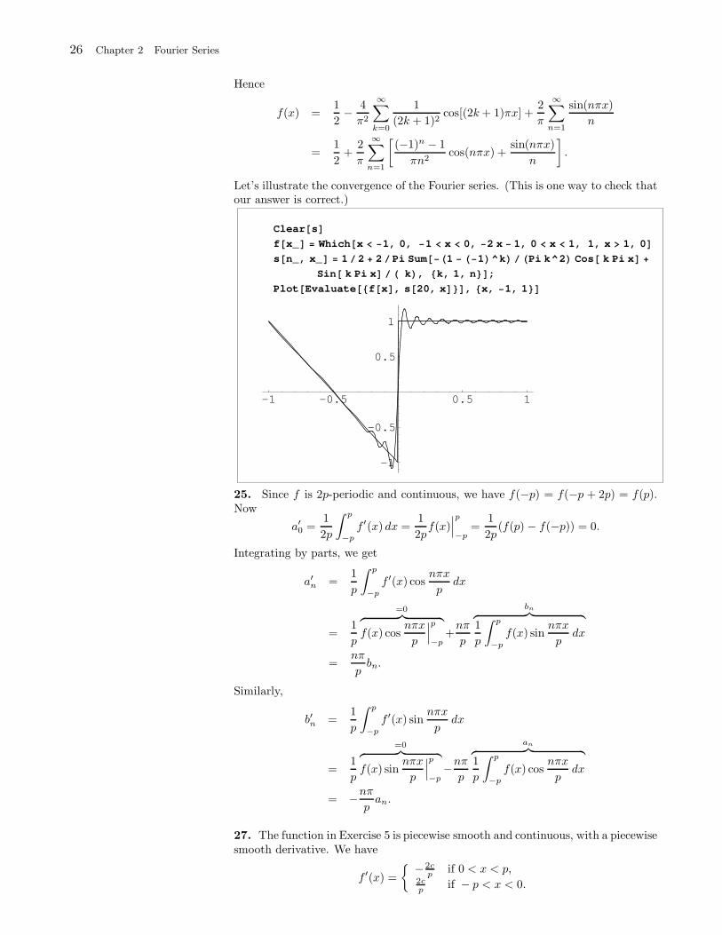
Hence
f(x) =1
2− 4
π2
∞∑
k=0
1
(2k + 1)2cos[(2k+ 1)πx] +
2
π
∞∑
n=1
sin(nπx)
n
=1
2+
2
π
∞∑
n=1
[(−1)n − 1
πn2cos(nπx) +
sin(nπx)
n
].
Let’s illustrate the convergence of the Fourier series. (This is one way to check thatour answer is correct.)
Clear s
f x_ Which x 1, 0, 1 x 0, 2 x 1, 0 x 1, 1, x 1, 0
s n_, x_ 1 2 2 Pi Sum 1 1 ^k Pi k^2 Cos k Pi x
Sin k Pi x k , k, 1, n ;
Plot Evaluate f x , s 20, x , x, 1, 1
-1 -0.5 0.5 1
-1
-0.5
0.5
1
25. Since f is 2p-periodic and continuous, we have f(−p) = f(−p + 2p) = f(p).Now
a′0 =1
2p
∫ p
−p
f ′(x) dx =1
2pf(x)
∣∣∣p
−p=
1
2p(f(p) − f(−p)) = 0.
Integrating by parts, we get
a′n =1
p
∫ p
−p
f ′(x) cosnπx
pdx
=1
p
=0︷ ︸︸ ︷f(x) cos
nπx
p
∣∣∣p
−p+nπ
p
bn︷ ︸︸ ︷1
p
∫ p
−p
f(x) sinnπx
pdx
=nπ
pbn.
Similarly,
b′n =1
p
∫ p
−p
f ′(x) sinnπx
pdx
=1
p
=0︷ ︸︸ ︷f(x) sin
nπx
p
∣∣∣p
−p−nπp
an︷ ︸︸ ︷1
p
∫ p
−p
f(x) cosnπx
pdx
= −nπpan.
27. The function in Exercise 5 is piecewise smooth and continuous, with a piecewisesmooth derivative. We have
f ′(x) =
−2cp
if 0 < x < p,2cp
if − p < x < 0.
Section 2.3 Fourier Series of Functions with Arbitrary Periods 27
The Fourier series of f ′ is obtained by differentiating term by term the Fourierseries of f (by Exercise 26). So
f ′(x) =8c
π2
∞∑
k=0
−1
(2k + 1)2(2k + 1)π
psin
(2k + 1)π
px = − 8c
pπ
∞∑
k=0
1
2k + 1sin
(2k + 1)π
px.
Now the function in Exercise 1 is obtained by multiplying f ′(x) by − p2c
. So toobtain the Fourier series in Exercise 1, we multiply the Fourier series of f ′ by − p
2cand get
4
π
∞∑
k=0
1
2k + 1sin
(2k + 1)π
px.
29. The function in Exercise 8 is piecewise smooth and continuous, with a piecewisesmooth derivative. We have
f ′(x) =
− cd
if 0 < x < d,0 if d < |x| < p,cd if − d < x < 0.
The Fourier series of f ′ is obtained by differentiating term by term the Fourier seriesof f (by Exercise 26). Now the function in this exercise is obtained by multiplyingf ′(x) by −d
c . So the desired Fourier series is
−dcf ′(x) = −d
c
2cp
dπ2
∞∑
n=1
1 − cos dnπp
n2
(−nπp
)sin
nπ
px =
2
π
∞∑
n=1
1 − cos dnπp
nsin
nπ
px.
31. (a) If limn→∞ cos nx = 0 for some x, then any subsequence of (cos nx) also con-verges to 0, in particular, limn→∞ cos(2nx) = 0. Furthermore, limn→∞ cos2 nx = 0.
But cos2 nx = 1+cos(2nx)2 , and taking the limit as n → ∞ on both sides we get
0 = 1+02
or 0 = 1/2, which is obviously a contradiction. Hence limn→∞ cosnx = 0holds for no x.(b) If
∑n=0 ∞ cosnx converges for some x, then by the nth term test, we must
have limn→∞ cos nx = 0. But this limit does not hold for any x; so the series doesnot converge for any x.
33. The function F (x) is continuous and piecewise smooth with F ′(x) = f(x) at allthe points where f is continuous (see Exercise 25, Section 2.1). So, by Exercise 26,if we differentiate the Fourier series of F , we get the Fourier series of f . Write
F (x) = A0 +
∞∑
n=1
(An cos
nπ
px+ Bn sin
nπ
px
)
and
f(x) =
∞∑
n=1
(an cos
nπ
px+ bn sin
nπ
px
).
Note that the a0 term of the Fourier series of f is 0 because by assumption∫ 2p
0 f(x) dx = 0. Differentiate the series for F and equate it to the series for fand get
∞∑
n=1
(−An
nπ
psin
nπ
px+
nπ
pBn cos
nπ
px
)=
∞∑
n=1
(an cos
nπ
px+ bn sin
nπ
px
).
Equate the nth Fourier coefficients and get
−Annπ
p= bn ⇒ An = − p
nπbn;
Bnnπ
p= an ⇒ Bn =
p
nπan.
28 Chapter 2 Fourier Series
This derives the nth Fourier coefficients of F for n ≥ 1. To get A0, note thatF (0) = 0 because of the definition of F (x) =
∫ x
0f(t) dt. So
0 = F (0) = A0 +
∞∑
n=1
An = A0 +
∞∑
n=1
− p
nπbn;
and so A0 =∑∞
n=1p
nπ bn. We thus obtained the Fourier series of F in terms of theFourier coefficients of f ; more precisely,
F (x) =p
π
∞∑
n=1
bnn
+
∞∑
n=1
(− p
nπbn cos
nπ
px+
p
nπan sin
nπ
px
).
The point of this result is to tell you that, in order to derive the Fourier series ofF , you can integrate the Fourier series of f term by term. Furthermore, the onlyassumption on f is that it is piecewise smooth and integrates to 0 over one period(to guarantee the periodicity of F .) Indeed, if you start with the Fourier series off ,
f(t) =
∞∑
n=1
(an cos
nπ
pt + bn sin
nπ
pt
),
and integrate term by term, you get
F (x) =
∫ x
0
f(t) dt =
∞∑
n=1
(an
∫ x
0
cosnπ
pt dt+ bn
∫ x
0
sinnπ
pt dt
)
=
∞∑
n=1
(an
( p
nπ
)sin
nπ
pt∣∣∣x
0dt+ bn
(− p
nπ
)cos
nπ
pt∣∣∣x
0
)
=p
π
∞∑
n=1
bnn
+
∞∑
n=1
(− p
nπbn cos
nπ
px+
p
nπan sin
nπ
px
),
as derived earlier. See the following exercise for an illustration.
Section 2.4 Half-Range Expansions: The Cosine and Sine Series 29
Solutions to Exercises 2.4
1. The even extension is the function that is identically 1. So the cosine Fourierseries is just the constant 1. The odd extension yields the function in Exercise 1,Section 2.3, with p = 1. So the sine series is
4
π
∞∑
k=0
sin((2k + 1)πx)
2k+ 1.
This is also obtained by evaluating the integral in (4), which gives
bn = 2
∫ 1
0
sin(nπx) dx = − 2
nπcosnπx
∣∣∣1
0=
2
nπ(1 − (−1)n).
3. The even extension is the function in Exercise 4, Section 2.3, with p = 1. Sothe cosine Fourier series is
1
3− 4
π2
∞∑
n=1
(−1)n+1 1
n2cosnπx.
In evaluating the sine Fourier coefficients, we will use the formula
∫x2 sin ax dx = −
((−2 + a2 x2
)cos(a x)
a3
)+
2 x sin(a x)
a2+C (a 6= 0),
which is obtained using integration by parts. For n ≥ 1, we have
bn = 2
∫ 1
0
x2 sin(nπx) dx
= −2
[(−2 + (nπ)2 x2) cos(nπ x)
(nπ)3− 2 x sin(nπ x)
(nπ)2
] ∣∣∣1
0
= −2
[(−2 + (nπ)2)(−1)n
(nπ)3+
2
(nπ)3
]
= 2
[(−1)n+1
nπ+
2
(nπ)3((−1)n − 1)
].
Thus the sine series representation
2
∞∑
n=1
[(−1)n+1
nπ+
2
(nπ)3((−1)n − 1)
]sin(nπx).
5. (a) Cosine series:
a0 =1
p
∫ b
a
dx =b− a
p;
an =2
p
∫ b
a
cosnπx
pdx =
2
p
p
nπ
(sin
nπb
p− sin
nπa
p
);
thus the even extension has the cosine series
fe(x) =b− a
p+
2
π
∞∑
n=1
1
n
(sin
nπb
p− sin
nπa
p
)cos
nπx
p.
Sine series:
bn =2
p
∫ b
a
sinnπx
pdx =
2
p
p
nπ
(cos
nπa
p− cos
nπb
p
);
30 Chapter 2 Fourier Series
thus the odd extension has the sine series
fo(x) =2
π
∞∑
n=1
1
n
(cos
nπa
p− cos
nπb
p
)sin
nπx
p.
7. The even extension is the function | cosx|. This is easily seen by plotting thegraph. The cosine series is (Exercise 8, Section 2.2):
| cosx| =2
π− 4
π
∞∑
n=1
(−1)n
(2n)2 − 1cos(2nx).
Sine series:
bn =4
π
∫ π2
0
cosx sin 2nx dx
=2
π
∫ π2
0
[sin(1 + 2n)x− sin(1 − 2n)x)] dx
=2
π
[ 1
−1 + 2n+
1
1 + 2n−
=0︷ ︸︸ ︷cos(
(−1 + 2n) π
2)
−1 + 2n−
=0︷ ︸︸ ︷cos(
(1 + 2n) π
2)
1 + 2n
]
=8
π
n
4n2 − 1;
thus the odd extension has the sine series
fo(x) =8
π
∞∑
n=1
n
4n2 − 1sin 2nx.
9. We have
bn = 2
∫ 1
0
x(1 − x) sin(nπx) dx.
To evaluate this integral, we will use integration by parts to derive the followingtwo formulas: for a 6= 0,
∫x sin(ax) dx = −x cos(a x)
a+
sin(a x)
a2+ C,
and ∫x2 sin(ax) dx =
2 cos(a x)
a3− x2 cos(a x)
a+
2 x sin(a x)
a2+ C.
So∫x(1 − x) sin(ax) dx
=−2 cos(a x)
a3− x cos(a x)
a+x2 cos(a x)
a+
sin(a x)
a2− 2 x sin(a x)
a2+C.
Applying the formula with a = nπ, we get
∫ 1
0
x(1 − x) sin(nπx) dx
=−2 cos(nπ x)
(nπ)3− x cos(nπ x)
nπ+x2 cos(nπ x)
nπ+
sin(nπ x)
(nπ)2− 2 x sin(nπ x)
(nπ)2
∣∣∣1
0
=−2 ((−1)n − 1)
(nπ)3− (−1)n
nπ+
(−1)n
nπ=
−2 ((−1)n − 1)
(nπ)3
=
4(nπ)3 if n is odd,
0 if n is even.
Section 2.4 Half-Range Expansions: The Cosine and Sine Series 31
Thus
bn =
8(nπ)3 if n is odd,
0 if n is even,
Hence the sine series in
8
π3
∞∑
k=0
sin(2k + 1)πx
(2k + 1)3.
b k_ 8 Pi^3 1 2 k 1 ^3;
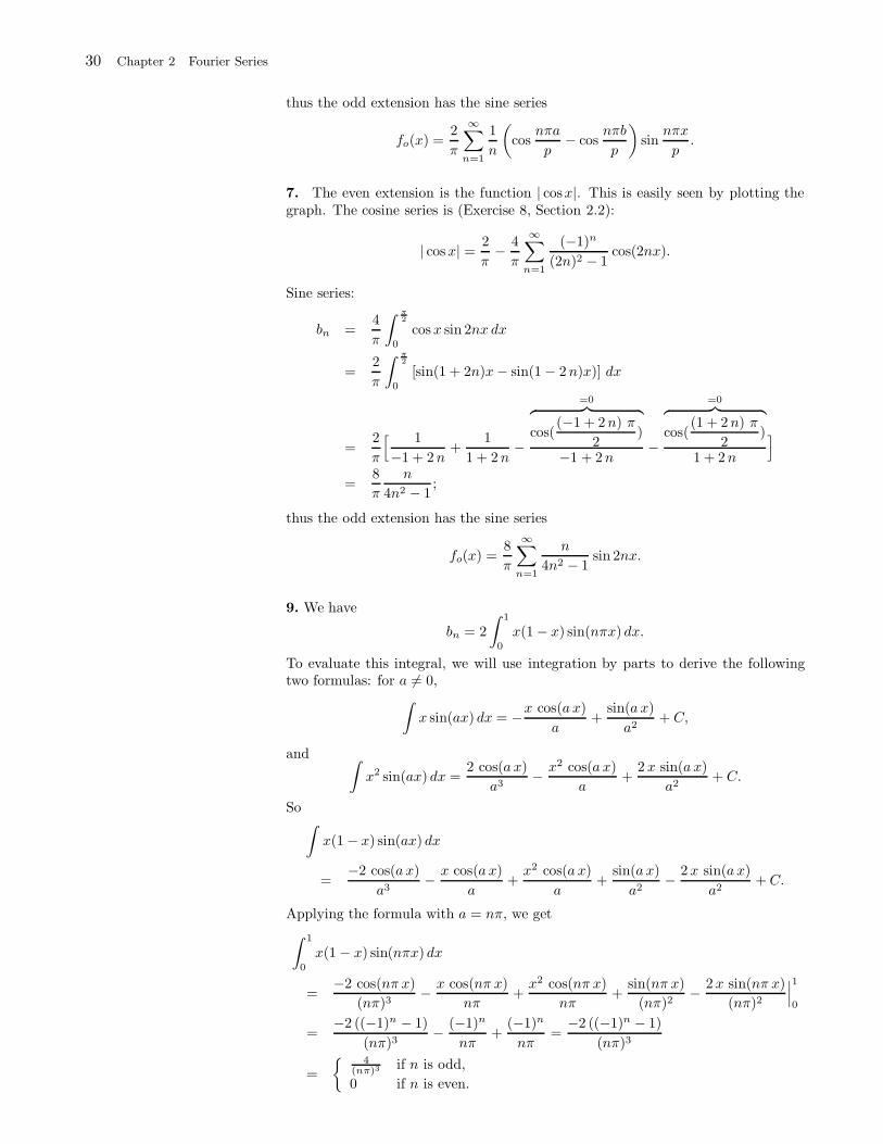
ss n_, x_ : Sum b k Sin 2 k 1 Pi x , k, 0, n ;
partialsineseries Table ss n, x , n, 1, 5 ;
f x_ x 1 x
Plot Evaluate partialsineseries, f x , x, 0, 1
0.2 0.4 0.6 0.8 1
0.05
0.1
0.15
0.2
0.25
Perfect!
11. The function is its own sine series.
13. We have
sinπx cosπx =1
2sin 2πx.
This yields the desired 2-periodic sine series expansion.
15. We have
bn = 2
∫ 1
0
ex sinnπx dx = =2ex
1 + (nπ)2(sinnπx− nπ cos nπx)
∣∣∣1
0
=2e
1 + (nπ)2(nπ(−1)n+1
)+
2nπ
1 + (nπ)2
=2nπ
1 + (nπ)2(1 + e(−1)n+1
).
Hence the sine series is
∞∑
n=1
2nπ
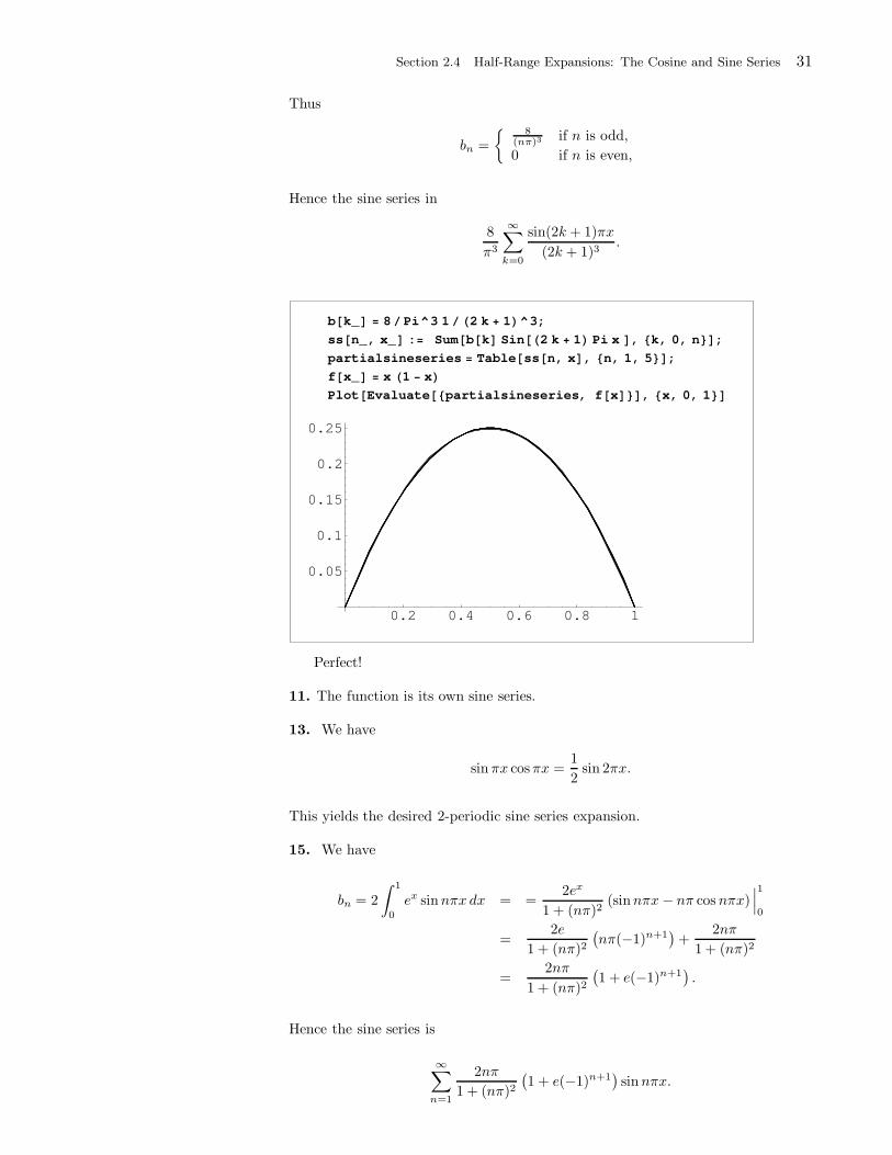
1 + (nπ)2(1 + e(−1)n+1
)sinnπx.
32 Chapter 2 Fourier Series
17. (b) Sine series expansion:
bn =2
p
∫ a
0
h
ax sin
nπx
pdx+
2
p
∫ p
a
h
a− p(x− p) sin
nπx
pdx
=2h
ap
[− x
p
nπcos
nπx
p
∣∣∣a
0+
p
nπ
∫ a
0
cosnπx
pdx]
+2h
(a − p)p
[(x− p)
(−p)nπ
cos(nπ x
p)∣∣∣p
a+
∫ p
a
p
nπcos
nπ x
pdx]
=2h
pa
[−apnπ
cosnπa
p+
p2
(nπ)2sin
nπa
p
]
+2h
(a − p)p
[ pnπ
(a− p) cosnπa
p− p2
(nπ)2sin
nπa
p
]
=2hp
(nπ)2sin
nπa
p
[1a− 1
a− p
]
=2hp2
(nπ)2(p− a)asin
nπa
p.
Hence, we obtain the given Fourier series.
Solutions to Exercises 2.5
1. We have
f(x) =
1 if 0 < x < 1,−1 if − 1 < x < 0;
The Fourier series representation is
f(x) =4
π
∞∑
k=0
1
2k + 1sin(2k + 1)πx.
The mean square error (from (5)) is
EN =1
2
∫ 1
−1
f2(x) dx− a20 −
1
2
N∑
n=1
(a2n + b2n).
In this case, an = 0 for all n, b2k = 0, b2k+1 = 4π(2k+1)
, and
1
2
∫ 1
−1
f2(x) dx =1
2
∫ 1
−1
dx = 1.
So
E1 = 1 − 1
2(b21) = 1 − 8
π2≈ 0.189.
Since b2 = 0, it follows that E2 = E1. Finally,
E1 = 1 − 1
2(b21 + b23) = 1 − 8
π2− 8
9 π2≈ 0.099.
3. We have f(x) = 1− (x/π)2 for −π < x < π. Its Fourier series representation is
f(x) =2
3+ 4
∞∑
n=1
(−1)n+1
(nπ)2cosnx.
Thus a0 = 23, an = 4 (−1)n+1
(nπ)2, and bn = 0 for all n ≥ 1. The mean square error
Section 2.5 Mean Square Approximation and Parseval’s Identity 33
(from (5)) is
EN =1
2π
∫ π
−π
f2(x) dx− a20 −
1
2
N∑
n=1
(a2n + b2n)
=1
2π
∫ π
−π
(1 − (x/π)2
)2dx− 4
9− 8
π4
N∑
n=1
1
n4
=1
2π
∫ π
−π
(1 − 2
x2
π2+x4
π4
)dx− 4
9− 8
π4
N∑
n=1
1
n4
=1
π
[x− 2 x3
3π2+
x5
5π4
]∣∣∣π
0− 4
9− 8
π4
N∑
n=1
1
n4
= 1 − 2
3+
1
5− 4
9− 8
π4
N∑
n=1
1
n4
=4
45− 8
π4
N∑
n=1
1
n4.
So
E1 =4
45− 8
π4≈ .0068;
E2 = E1 −8
π4
1
24≈ .0016;
E3 = E2 −8
π4
1
34≈ .0006.
5. We have
EN =1
2
∫ 1
−1
f2(x) dx− a20 −
1
2
N∑
n=1
(a2n + b2n)
= 1 − 1
2
N∑
n=1
b2n = 1 − 8
π2
∑
1≤n odd≤N
1
n2.
With the help of a calculator, we find that E39 = .01013 and E41 = .0096. So takeN = 41.
7. (a) Parseval’s identity with p = π:
1
2π
∫ π
−π
f(x)2 dx = a20 +
1
2
∞∑
n=1
(a2n + b2n).
Applying this to the given Fourier series expansion, we obtain
1
2π
∫ π
−π
x2
4dx =
1
2
∞∑
n=1
1
n2⇒ π2
12=
1
2
∞∑
n=1
1
n2⇒ π2
6=
∞∑
n=1
1
n2.
For (b) and (c) see the solution to Exercise 17, Section 2.3.
9. We have f(x) = π2x− x3 for −π < x < π and, for n ≥ 1, bn = 12n3 (−1)n+1. By
34 Chapter 2 Fourier Series
Parseval’s identity
1
2
∞∑
n=1
(12
n3
)2
=1
2π
∫ π
−π
(π2x− x3
)2
=1
π
∫ π
0
(π4x2 − 2π2x4 + x6
)dx
=1
π
(π4
3x3 − 2π2
5x5 +
x7
7
) ∣∣∣π
0
= π6
(1
3− 2
5+
1
7
)=
8
105π6.
Simplifying, we find that
ζ(6) =
∞∑
n=1
1
n6=
(8)(2)
(105)(144)π6 =
π6
945.
13. For the given function, we have bn = 0 and an = 1n2 . By Parseval’s identity,
we have
1
2π
∫ π
−π
f2(x) dx =1
2
∞∑
n=1
1
n4⇒
∫ π
−π
f2(x) dx = π
∞∑
n=1
1
n4= πζ(4) =
π5
90,
where we have used the table preceding Exercise 7 to compute ζ(4).
15. Let us write the terms of the function explicitly. We have
f(x) =
∞∑
n=0
cosnx
2n= 1 +
cosx
2+
cos 2x
22+ · · · .
Thus for the given function, we have
bn = 0 for all n, a0 = 1, an =1
2nfor n ≥ 1.
By Parseval’s identity, we have
1
2π
∫ π
−π
f2(x) dx = a20 +
1
2
∞∑
n=1
a2n
= 1 +1
2
∞∑
n=1
1
(2n)2=
1
2+
1
2+
1
2
∞∑
n=1
1
4n
=1
2+
1
2
∞∑
n=0
1
4n.
To sum the last series, we use a geometric series: if |r| < 1,
∞∑
n=0
rn =1
1 − r.
Hence∞∑
n=0
1
4n=
1
1 − 14
=4
3,
and so ∫ π
−π
f2(x) dx = 2π(1
2+
1
2
4
3) =
7π
3.
Section 2.5 Mean Square Approximation and Parseval’s Identity 35
17. For the given function, we have
a0 = 1, an =1
3n, bn =
1
nfor n ≥ 1.
By Parseval’s identity, we have
1
2π
∫ π
−π
f2(x) dx = a20 +
1
2
∞∑
n=1
(a2n + b2n)
= 1 +1
2
∞∑
n=1
(1
(3n)2+
1
n2)
=1
2+
1
2+
1
2
∞∑
n=1
1
9n+
1
2
∞∑
n=1
1
n2
=1
2+
1
2
∞∑
n=0
1
9n+
1
2
∞∑
n=1
1
n2.
Using a geometric series, we find
∞∑
n=0
1
9n=
1
1 − 19
=9
8.
By Exercise 7(a),∞∑
n=1
1
n2=π2
6.
So ∫ π
−π
f2(x) dx = 2π(1
2+
1
2
9
8+
1
2
π2
6) =
17π
8+π3
6.
36 Chapter 2 Fourier Series
Solutions to Exercises 2.6
1. From Example 1, for a 6= 0,±i,±2i,±3i, . . .,
eax =sinhπa
π
∞∑
n=−∞
(−1)n
a− ineinx (−π < x < π);
consequently,
e−ax =sinhπa
π
∞∑
n=−∞
(−1)n
a+ ineinx (−π < x < π),
and so, for −π < x < π,
cosh ax =eax + e−ax
2
=sinhπa
2π
∞∑
n=−∞(−1)n
(1
a+ in+
1
a− in
)einx
=a sinhπa
π
∞∑
n=−∞
(−1)n
n2 + a2einx.
3. In this exercise, we will use the formulas cosh(iax) = cos ax and sinh(iax) =i sin ax, for all real a and x. (An alternative method is used in Exercise 4.) Toprove these formulas, write
cosh(iax) =eiax + e−iax
2= cos ax,
by Euler’s identity. Similarly,
sinh(iax) =eiax − e−iax
2= i sin ax.
If a is not an integer, then ia 6= 0,±i,±2i,±3i, . . ., and we may apply the result ofExercise 1 to expand eiax in a Fourier series:
cos(ax) = cosh(iax) =(ia) sinh(iπa)
π
∞∑
n=−∞
(−1)n
n2 + (ia)2einx
=−a sin(πa)
π
∞∑
n=−∞
(−1)n
n2 − a2einx.
5. Use identities (1); then
cos 2x+ 2 sin 3x =e2ix + e−2ix
2+ 2
e3ix − e−3ix
2i
= ie−3ix +e−2ix
2+e2ix
2− ie3ix.
7. You can use formulas (5)–(8) to do this problem, or you can start with the
Section 2.6 Complex Form of Fourier Series 37
Fourier series in Exercise 3 and rewrite it as follows:
cos ax =−a sin(πa)
π
∞∑
n=−∞
(−1)neinx
n2 − a2
=−a sin(πa)
π
−1∑
n=−∞
(−1)neinx
n2 − a2− a sin(πa)
π
1
−a2− a sin(πa)
π
∞∑
n=1
(−1)neinx
n2 − a2
=sin(πa)
πa− a sin(πa)
π
∞∑
n=1
(−1)−ne−inx
(−n)2 − a2− a sin(πa)
π
∞∑
n=1
(−1)neinx
n2 − a2
=sin(πa)
πa− a sin(πa)
π
∞∑
n=1
(−1)n
=2 cosnx︷ ︸︸ ︷einx + e−inx
n2 − a2
=sin(πa)
πa− 2
a sin(πa)
π
∞∑
n=1
(−1)n cosnx
n2 − a2.
9. If m = n then
1
2p
∫ p
−p
ei mπp xe−i nπ
p xdx =1
2p
∫ p
−p
ei mπp xe−i mπ
p xdx =1
2p
∫ p
−p
dx = 1.
If m 6= n, then
1
2p
∫ p
−p
ei mπp xe−i nπ
p xdx =1
2p
∫ p
−p
ei (m−n)πp xdx
=−i
2(m− n)πei
(m−n)πp x
∣∣∣p
−p
=−i
2(m− n)π
(ei(m−n)π − e−i(m−n)π
)
=−i
2(m− n)π(cos[(m− n)π] − cos[−(m− n)π]) = 0.
11. The function in Example 1 is piecewise smooth on the entire real line andcontinuous at x = 0. By the Fourier series representation theorem, its Fourier seriesconverges to the value of the function at x = 0. Putting 4x=04 in the Fourier serieswe thus get
f(0) = 1 =sinhπa
π
∞∑
n=−∞
(−1)n
a2 + n2(a+ in).
The doubly infinite sum is to be computed by taking symmetric partial sums, asfollows:
∞∑
n=−∞
(−1)n
a2 + n2(a+ in) = lim
N→∞
N∑
n=−N
(−1)n
a2 + n2(a+ in)
= a limN→∞
N∑
n=−N
(−1)n
a2 + n2+ i lim
N→∞
N∑
n=−N
(−1)nn
a2 + n2.
ButN∑
n=−N
(−1)nn
a2 + n2= 0,
because the summand is an odd function of n. So
1 =sinhπa
π
∞∑
n=−∞
(−1)n
a2 + n2(a + in) =
a sinhπa
π
∞∑
n=−∞
(−1)n
a2 + n2,
38 Chapter 2 Fourier Series
which is equivalent to the desired identity.
13. (a) At points of discontinuity, the Fourier series in Example 1 converges tothe average of the function. Consequently, at x = π the Fourier series converges toeaπ+e−aπ
2 = cosh(aπ). Thus, plugging x = π into the Fourier series, we get
cosh(aπ) =sinh(πa)
π
∞∑
n=−∞
(−1)n
a2 + n2(a+ in)
=(−1)n
︷︸︸︷einπ =
sinh(πa)
π
∞∑
n=−∞
(a+ in)
a2 + n2.
The sum∑∞
n=−∞in
a2+n2 is the limit of the symmetric partial sums
i
N∑
n=−N
n
a2 + n2= 0.
Hence∑∞
n=−∞in
a2+n2 = 0 and so
cosh(aπ) =sinh(πa)
π
∞∑
n=−∞
a
a2 + n2⇒ coth(aπ) =
a
π
∞∑
n=−∞
1
a2 + n2,
upon dividing both sides by sinh(aπ). Setting t = aπ, we get
coth t =t
π2
∞∑
n=−∞
1
( tπ )2 + n2
=
∞∑
n=−∞
t
t2 + (πn)2,
which is (b). Note that since a is not an integer, it follows that t is not of the formkπi, where kis an integer.
15. (a) This is straightforward. Start with the Fourier series in Exercise 1: Fora 6= 0,±i,±2i,±3i, . . ., and −π < x < π, we have
cosh ax =a sinhπa
π
∞∑
n=−∞
(−1)n
n2 + a2einx.
On the left side, we have
1
2π
∫ π
−π
cosh2(ax) dx =1
π
∫ π
0
cosh(2ax) + 1
2dx
=1
2π
[x+
1
2asinh(2ax)
]∣∣∣π
0=
1
2π
[π +
1
2asinh(2aπ)
].
On the right side of Parseval’s identity, we have
(a sinhπa)2
π2
∞∑
n=−∞
1
(n2 + a2)2.
Hence1
2π
[π +
1
2asinh(2aπ)
]=
(a sinhπa)2
π2
∞∑
n=−∞
1
(n2 + a2)2.
Simplifying, we get
∞∑
n=−∞
1
(n2 + a2)2=
π
2(a sinhπa)2[π +
1
2asinh(2aπ)
].
(b) This part is similar to part (a). Start with the Fourier series of Exercise 2: Fora 6= 0,±i,±2i,±3i, . . ., and −π < x < π, we have
sinh ax =i sinhπa
π
∞∑
n=−∞(−1)n n
n2 + a2einx.
Section 2.6 Complex Form of Fourier Series 39
On the left side, we have
1
2π
∫ π
−π
sinh2(ax) dx =1
π
∫ π
0
cosh(2ax) − 1
2dx
=1
2π
[− x+
1
2asinh(2ax)
]∣∣∣π
0=
1
2π
[− π +
1
2asinh(2aπ)
].
On the right side of Parseval’s identity, we have
sinh2 πa
π2
∞∑
n=−∞
n2
(n2 + a2)2.
Hence1
2π
[− π +
1
2asinh(2aπ)
]=
sinh2(πa)
π2
∞∑
n=−∞
n2
(n2 + a2)2.
Simplifying, we get
∞∑
n=−∞
n2
(n2 + a2)2=
π
2 sinh2(πa)
[− π +
1
2asinh(2aπ)
].
17. (a) In this exercise, we let a and b denote real numbers such that a2 + b2 6= 0.Using the linearity of the integral of complex-valued functions, we have
I1 + iI2 =
∫eax cos bx dx+ i
∫eax sin bx dx
=
∫(eax cos bx+ ieax sin bx) dx
=
∫eax
eibx
︷ ︸︸ ︷(cos bx+ i sin bx) dx
=
∫eaxeibx dx =
∫ex(a+ib) dx
=1
a+ ibex(a+ib) +C,
where in the last step we used the formula∫eαx dx = 1
αeαx +C (with α = a+ ib),
which is valid for all complex numbers α 6= 0 (see Exercise 19 for a proof).(b) Using properties of the complex exponential function (Euler’s identity and thefact that ez+w = ezew), we obtain
I1 + iI2 =1
a+ ibex(a+ib) +C
=(a+ ib)
(a+ ib) · (a+ ib)eaxeibx +C
=a− ib
a2 + b2eax(cos bx+ i sin bx
)+ C
=eax
a2 + b2[(a cos bx+ b sin bx
)+ i(− b cos bx+ a sin bx
)]+ C.
(c) Equating real and imaginary parts in (b), we obtain
I1 =eax
a2 + b2(a cos bx+ b sin bx
)
and
I2 =eax
a2 + b2(− b cos bx+ a sin bx
).
40 Chapter 2 Fourier Series
19. The purpose of this exercise is to show you that the familiar formula fromcalculus for the integral of the exponential function,
∫eax dx =
1
aeax + C,
holds for all nonzero complex numbers a. Note that this formula is equivalent to
d
dxeax = aeax,
where the derivative of ddxe
ax means
d
dxeax =
d
dx
(Re (eax) + i Im (eax)
)=
d
dxRe (eax) + i
d
dxIm (eax).
Write a = α+ iβ, where α and β are real numbers. Then
eax = ex(α+iβ) = eαxeiβx
= eαx cos βx+ ieαx sinβx.
So
d
dxeax =
d
dxeαx cos βx+ i
d
dxeαx sinβx
= αeαx cosβx − βeαx sinβx+ i(αeαx sinβx + βeαx cosβx
)
= eαx(α cosβx − β sinβx + i
(α sinβx+ β cosβx
))
= eαx(cos βx+ i sinβx)(α + iβ)
= aeαxeiβx = aeαx+iβxaeiax,
as claimed.
21. By Exercise 19,
∫ 2π
0
(eit + 2e−2it
)dt =
1
ieit +
2
−2ie−2it
∣∣∣2π
0
= −i=1︷︸︸︷e2πi +i
=1︷ ︸︸ ︷e−2πi −(−i+ i) = 0.
Of course, this result follows from the orthogonality relations of the complex expo-nential system (formula (11), with p = π).
23. First note that1
cos t− i sin t=
1
e−it= eit.
Hence ∫1
cos t− i sin tdt =
∫eitdt = −ieit + C = sin t − i cos t+ C.
25. First note that
1 + it
1 − it=
(1 + it)2
(1 − it)(1 + it)=
1 − t2 + 2it
1 + t2=
1 − t2
1 + t2+ i
2t
1 + t2.
Hence∫
1 + it
1 − itdt =
∫1 − t2
1 + t2dt+ i
∫2t
1 + t2dt
=
∫(−1 +
2
1 + t2dt+ i
∫2t
1 + t2dt
= −t + 2 tan−1 t + i ln(1 + t2) +C.
Section 2.7 Forced Oscillations 41
Solutions to Exercises 2.7
1. (a) General solution of y′′ + 2y′ + y = 0. The characteristic equation isλ2 +2λ+1 = 0 or (λ+1)2 = 0. It has one double characteristic root λ = −1. Thusthe general solution of the homogeneous equation y′′ + 2y′ + y = 0 is
y = c1e−t + c2te
−t.
To find a particular solution of y′′ + 2y′ + y = 25 cos 2t, we apply Theorem 1 withµ = 1, c = 2, and k = 1. The driving force is already given by its Fourier series:We have bn = an = 0 for all n, except a2 = 25. So αn = βn = 0 for all n,except α2 = A2a2
A22+B2
2and β2 = B2a2
A22+B2
2, where A2 = 1 − 22 = −3 and B2 = 4.
Thus α2 = −7525 = −3 and β2 = 100
25 = 4, and hence a particular solution isyp = −3 cos 2t+ 4 sin 2t. Adding the general solution of the homogeneous equationto the particular solution, we obtain the general solution of the differential equationy′′ + 2y′ + y = 25 cos 2t
y = c1e−t + c2te
−t − 3 cos 2t+ 4 sin 2t.
(b) Since limt→∞ c1e−t + c2te
−t = 0, it follows that the steady-state solution is
ys = −3 cos 2t+ 4 sin 2t.
3. (a) General solution of 4y′′ + 4y′ + 17y = 0. The characteristic equation is4λ2 + 4λ + 17 = 0. Its characteristic roots are
λ =−2 ±
√4 − (4)(17)
4=
−2 ±√−64
4= −1
2± 2i.
Thus the general solution of the homogeneous equation is
y = c1e−t/2 cos 2t+ c2e
−t/2 sin 2t.
It is easy to see that y = 1/17 is a particular solution of 4y′′ +4y′ +17y = 1. (Thisalso follows from Theorem 1.) Hence the general solution is
y = c1e−t/2 cos 2t+ c2e
−t/2 sin 2t+1
17.
(b) Since limt→∞ c1e−t/2 cos 2t+ c2e
−t/2 sin 2t = 0, it follows that the steady-statesolution is
ys =1
17.
5. (a) To find a particular solution (which is also the steady-state solution) ofy′′ + 4y′ + 5y = sin t− 1
2 sin 2t, we apply Theorem 1 with µ = 1, c = 4, and k = 5.The driving force is already given by its Fourier series: We have bn = an = 0 forall n, except b1 = 1 and b2 = −1/2. So αn = βn = 0 for all n, except, possibly, α1,α2, β1, and beta2. We have A1 = 4, A2 = 1, B1 = 4, and B2 = 8. So
α1 =−B1b1A2
1 + B21
=−4
32= −1
8,
α2 =−B2b2A2
2 + B22
=4
65=
4
65,
β1 =A1b1
A21 + B2
1
=4
32=
1
8,
β2 =A2b2
A22 + B2
2
=−1/2
65= − 1
130.
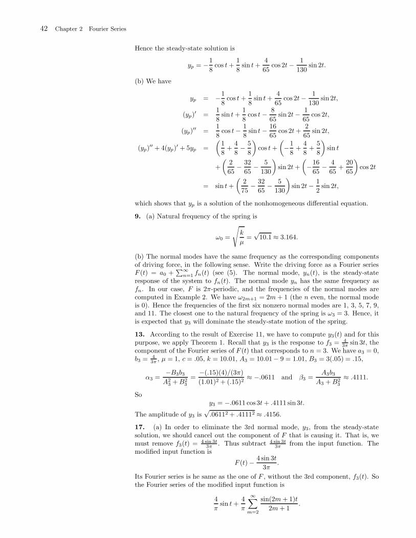
42 Chapter 2 Fourier Series
Hence the steady-state solution is
yp = −1
8cos t+
1
8sin t+
4
65cos 2t− 1
130sin 2t.
(b) We have
yp = −1
8cos t +
1
8sin t+
4
65cos 2t− 1
130sin 2t,
(yp)′ =1
8sin t+
1
8cos t − 8
65sin2t− 1
65cos 2t,
(yp)′′ =
1
8cos t− 1
8sin t − 16
65cos 2t+
2
65sin 2t,
(yp)′′ + 4(yp)′ + 5yp =
(1
8+
4
8− 5
8
)cos t+
(−1
8+
4
8+
5
8
)sin t
+
(2
65− 32
65− 5
130
)sin 2t+
(−16
65− 4
65+
20
65
)cos 2t
= sin t+
(2
75− 32
65− 5
130
)sin 2t− 1
2sin 2t,
which shows that yp is a solution of the nonhomogeneous differential equation.
9. (a) Natural frequency of the spring is
ω0 =
√k
µ=
√10.1 ≈ 3.164.
(b) The normal modes have the same frequency as the corresponding componentsof driving force, in the following sense. Write the driving force as a Fourier seriesF (t) = a0 +
∑∞n=1 fn(t) (see (5). The normal mode, yn(t), is the steady-state
response of the system to fn(t). The normal mode yn has the same frequency asfn. In our case, F is 2π-periodic, and the frequencies of the normal modes arecomputed in Example 2. We have ω2m+1 = 2m+ 1 (the n even, the normal modeis 0). Hence the frequencies of the first six nonzero normal modes are 1, 3, 5, 7, 9,and 11. The closest one to the natural frequency of the spring is ω3 = 3. Hence, itis expected that y3 will dominate the steady-state motion of the spring.
13. According to the result of Exercise 11, we have to compute y3(t) and for thispurpose, we apply Theorem 1. Recall that y3 is the response to f3 = 4
3π sin 3t, thecomponent of the Fourier series of F (t) that corresponds to n = 3. We have a3 = 0,b3 = 4
3π , µ = 1, c = .05, k = 10.01, A3 = 10.01− 9 = 1.01, B3 = 3(.05) = .15,
α3 =−B3b3A2
3 +B23
=−(.15)(4)/(3π)
(1.01)2 + (.15)2≈ −.0611 and β3 =
A3b3A3 +B2
3
≈ .4111.
Soy3 = −.0611 cos3t+ .4111 sin3t.
The amplitude of y3 is√.06112 + .41112 ≈ .4156.
17. (a) In order to eliminate the 3rd normal mode, y3, from the steady-statesolution, we should cancel out the component of F that is causing it. That is, wemust remove f3(t) = 4 sin 3t
3π . Thus subtract 4 sin 3t3π from the input function. The
modified input function is
F (t) − 4 sin 3t
3π.
Its Fourier series is he same as the one of F , without the 3rd component, f3(t). Sothe Fourier series of the modified input function is
4
πsin t+
4
π
∞∑
m=2
sin(2m+ 1)t
2m+ 1.
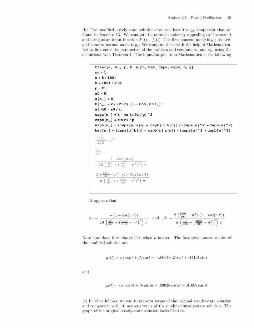
Section 2.7 Forced Oscillations 43
(b) The modified steady-state solution does not have the y3-component that wefound in Exercise 13. We compute its normal modes by appealing to Theorem 1and using as an input function F (t) − f3(t). The first nonzero mode is y1; the sec-ond nonzero normal mode is y5. We compute them with the help of Mathematica.Let us first enter the parameters of the problem and compute αn and βn, using thedefinitions from Theorem 1. The input/output from Mathematica is the following
Clear a, mu, p, k, alph, bet, capa, capb, b, y
mu 1;
c 5 100;
k 1001 100;
p Pi;
a0 0;
a n_ 0;
b n_ 2 Pi n 1 Cos n Pi ;
alph0 a0 k;
capa n_ k mu n Pi p ^2
capb n_ c n Pi p
alph n_ capa n a n capb n b n capa n ^2 capb n ^2
bet n_ capa n b n capb n a n capa n ^2 capb n ^2
1001
100n2
n
20
1 Cos n
10 n2
400
1001
100n2
2
2 1001
100n2 1 Cos n
n n2
400
1001
100n2
2
It appears that
αn =− (1 − cos(nπ))
10(
n2
400 +(
1001100 − n2
)2)π
and βn =2(
1001100 − n2
)(1 − cos(nπ))
n(
n2
400 +(
1001100 − n2
)2)π
Note how these formulas yield 0 when n is even. The first two nonzero modes ofthe modified solution are
y1(t) = α1 cos t+ β1 sin t = −.0007842 cos t+ .14131 sin t
and
y5(t) = α5 cos 5t+ β5 sin 5t− .00028 cos5t− .01698 sin5t.
(c) In what follows, we use 10 nonzero terms of the original steady-state solutionand compare it with 10 nonzero terms of the modified steady-state solution. Thegraph of the original steady-state solution looks like this:
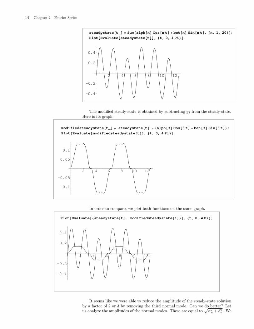
44 Chapter 2 Fourier Series
steadystate t_ Sum alph n Cos n t bet n Sin n t , n, 1, 20 ;
Plot Evaluate steadystate t , t, 0, 4 Pi
2 4 6 8 10 12
-0.4
-0.2
0.2
0.4
The modified steady-state is obtained by subtracting y3 from the steady-state.Here is its graph.
modifiedsteadystate t_ steadystate t alph 3 Cos 3 t bet 3 Sin 3 t ;
Plot Evaluate modifiedsteadystate t , t, 0, 4 Pi
2 4 6 8 10 12
-0.1
-0.05
0.05
0.1
In order to compare, we plot both functions on the same graph.
Plot Evaluate steadystate t , modifiedsteadystate t , t, 0, 4 Pi
2 4 6 8 10 12
-0.4
-0.2
0.2
0.4
It seems like we were able to reduce the amplitude of the steady-state solutionby a factor of 2 or 3 by removing the third normal mode. Can we do better? Letus analyze the amplitudes of the normal modes. These are equal to
√α2
n + β2n. We
Section 2.7 Forced Oscillations 45
have the following numerical values:
amplitudes N Table Sqrt alph n ^2 bet n ^2 , n, 1, 20
0.141312, 0., 0.415652, 0., 0.0169855, 0., 0.00466489, 0., 0.00199279, 0.,
0.00104287, 0., 0.000616018, 0., 0.000394819, 0., 0.000268454, 0., 0.000190924, 0.
It is clear from these values that y3 has the largest amplitude (which is whatwe expect) but y1 also has a relatively large amplitude. So, by removing thefirst component of F , we remove y1, and this may reduce the oscillations evenfurther. Let’s see the results. We will plot the steady-state solution ys, ys − y3,and ys − y1 − y3.
modifiedfurther t_ modifiedsteadystate t alph 1 Cos t bet 1 Sin t ;
Plot
Evaluate modifiedfurther t , steadystate t , modifiedsteadystate t , t, 0, 4 Pi
2 4 6 8 10 12
-0.4
-0.2
0.2
0.4
21. (a) The input function F (t) is already given by its Fourier series: F (t) =2 cos 2t+sin 3t. Since the frequency of the component sin 3t of the input function is3 and is equal to the natural frequency of the spring, resonance will occur (becausethere is no damping in the system). The general solution of y′′+9y = 2 cos 2t+sin 3tis y = yh +yp , where yh is the general solution of y′′ +9y = 0 and yp is a particularsolution of the nonhomogeneous equation. We have yh = c1 sin 3t + c2 cos 3t and,to find yp, we apply Exercise 20 and get
yp =
(a2
A2cos 2t+
b2A2
sin 2t
)+R(t),
where a2 = 2, b2 = 0, A2 = 9 − 22 = 5, an0 = 0, bn0 = 1, and
R(t) = − t
6cos 3t.
Hence
yp =2
5cos 2t− t
6cos 3t
and so the general solution is
y = c1 sin 3t+ c2 cos 3t+2
5cos 2t− t
6cos 3t.
46 Chapter 2 Fourier Series
(b) To eliminate the resonance from the system we must remove the component ofF that is causing resonance. Thus add to F (t) the function − sin 3t. The modifiedinput function becomes Fmodified(t) = 2 cos 2t.
25. The general solution is y = c1 sin 3t+ c2 cos 3t+ 25 cos 2t− t
6 cos 3t. Applyingthe initial condition y(0) = 0 we get c2 + 2
5 = 0 or c2 = −25 . Thus
y = c1 sin 3t− 2
5cos 3t+
2
5cos 2t− t
6cos 3t.
Applying the initial condition y′(0) = 0, we obtain
y′ = 3c1 cos 3t+6
5sin 3t− 6
5sin 2t− 1
6cos 3t+
t
2sin 3t,
y′(0) = 3c1 −1
6,
y′(0) = 0 ⇒ c1 =1
18.
Thus
y =1
18sin 3t− 2
5cos 3t+
2
5cos 2t− t
6cos 3t.
Section 2.9 Uniform Convergence and Fourier Series 47
Solutions to Exercises 2.9
1.
|fn(x)| =
∣∣∣∣sinnx√
n
∣∣∣∣ ≤1√n
→ 0 as n → ∞.
The sequence converges uniformly to 0 for all real x, because 1√n
controls its size
independently of x.
5. If x = 0 then fn(0) = 0 for all n. If x 6= 0, then applying l’Hospital’s rule, wefind
limn→∞
|fn(x)| = |x| limn→∞
n
e−nx= |x| lim
n→∞1
|x|e−n= 0.
The sequence does not converge uniformly on any interval that contains 0 becausefn( 1
n ) = e−1, which does not tend to 0.
6. As in Exercise 5, the sequence converges to pointwise to 0 for all x, but notuniformly on any interval that contains 0 because fn( 1
n ) = e−1 − e−2, which doesnot tend to 0.
7. The sequence converges to 0 for all x because the degree of n in the denominatoris greater than its degree in the numerator. For each n, the extreme points of fn(x)occur when f ′n(x) = 0 or
n− n3 x2
(1 + n2 x2)2 = 0 ⇒ n− n3x = 0 ⇒ x =
±1
n.
Since fn( 1n) = 1
2 the sequence does not converge to 0 uniformly on the interval[0, ∞) (or any interval that contains 0).
9.∣∣coskx
k2
∣∣ ≤ 1k2 = Mk for all x. Since
∑Mk <∞ (p-series with p > 1), the series
converges uniformly for all x.
14.∣∣ x10
∣∣ ≤ ( 910)k = Mk for all |x| ≤ 9. Since
∑( 910)k < ∞ (geometric series with
ratio 9/10 < 1), the series converges uniformly for all |x| ≤ 9.
17.∣∣∣ (−1)k
|x|+k2
∣∣∣ ≤ 1k2 = Mk for all x. Since
∑Mk < ∞ (p-series with p > 1), the
series converges uniformly for all x.
48 Chapter 2 Fourier Series
Solutions to Exercises 2.10
3. By Theorem 2(c), the series converges for all x 6= 2nπ. For x = 2nπ, the series∑∞k=1
cos 2knπ√k
=∑∞
k=11√k
is divergent.
5. The cosine part converges uniformly for all x, by the Weierstrass M -test. Thesine part converges for all x by Theorem 2(b). Hence the given series converges forall x.
9. (a) If limk→∞ sin kx = 0, then
limk→∞
sin2 kx = 0 ⇒ limk→∞
(1 − cos2 kx) = 0 ⇒ limk→∞
cos2 kx = 1 (∗).
Also, if limk→∞ sinkx = 0, then limk→∞ sin(k + 1)x) = 0. But sin(k + 1)x =sin kx cosx+ cos kx sinx, so
0 = limk→∞
(
→0︷ ︸︸ ︷sin kx cosx+cos kx sinx) ⇒ lim
k→∞cos kx sinx = 0
⇒ limk→∞
cos kx = 0 or sinx = 0.
By (*), cos kx does not tend to 0, so sinx = 0, implying that x = mπ. Consequently,if x 6= mπ, then limk → ∞ sin kx is not 0 and the series
∑∞k=1 sin kx does not
converge by the nth term test, which proves (b).
Section 3.1 Partial Differential Equations in Physics and Engineering 49
Solutions to Exercises 3.1
1. uxx + uxy = 2u is a second order, linear, and homogeneous partial differentialequation. ux(0, y) = 0 is linear and homogeneous.
3. uxx−ut = f(x, t) is a second order, linear, and nonhomogeneous (because of theright side) partial differential equation. ut(x, 0) = 2 is linear and nonhomogeneous.
5. utux+uxt = 2u is second order and nonlinear because of the term utux. u(0, t)+ux(0, t) = 0 is linear and homogeneous.
7. (a) uxx = uyy = 0, so uxx + uyy = 0.(b) uxx = 2, uyy = −2, so uxx + uyy = 0. (c) We have u = x
x2+y2 . So
ux =−x2 + y2
(x2 + y2)2 , uy =
−2 x y
(x2 + y2)2 ,
and
uxx =2(x3 − 3 x y2
)
(x2 + y2)3 , uyy =
−2(x3 − 3 xy2
)
(x2 + y2)3 ⇒ ∆u = uxx + uyy = 0.
(d) We have u = yx2+y2 . Switching x and y in (c), it follows immediately that
uy =−y2 + x2
(x2 + y2)2, ux =
−2 x y
(x2 + y2)2,
and
uyy =2(y3 − 3 y x2
)
(x2 + y2)3, uxx =
−2(y3 − 3 x2y
)
(x2 + y2)3⇒ ∆u = uxx + uyy = 0.
(e) We have u = ln(x2 + y2), so
ux =2 x
x2 + y2, uy =
2 y
x2 + y2,
and
uxx =−2
(x2 − y2
)
(x2 + y2)2 , uyy =
2(x2 − y2
)
(x2 + y2)2 ⇒ ∆u = uxx + uyy = 0.
(f) We have u = ey cos x, so
ux = −ey sin(x), uy = ey cos(x),
and
uxx = −ey cos(x), uyy = ey cos(x) ⇒ ∆u = uxx + uyy = 0.
(g) We have u = ln(x2 + y2) + ey cosx. Since u is the sum of two solutions ofLaplace’s equation (by (e) and (f)), it is itself a solution of Laplace’s equation.
9. (a) Let u(x, y) = eaxeby. Then
ux = aeaxeby
uy = beaxeby
uxx = a2eaxeby
uyy = b2eaxeby
uxy = abeaxeby.
50 Chapter 3 Partial Differential Equations in Rectangular Coordinates
So
Auxx + 2Buxy +Cuyy +Dux + Euy + Fu = 0
⇔ Aa2eaxeby + 2Babeaxeby +Cb2eaxeby
+Daeaxeby +Ebeaxeby + Feaxeby = 0
⇔ eaxeby(Aa2 + 2Bab +Cb2 +Da +Eb+ F
)= 0
⇔ Aa2 + 2Bab+ Cb2 +Da+ Eb+ F = 0,
because eaxeby 6= 0 for all x and y.(b) By (a), in order to solve
uxx + 2uxy + uyy + 2 ux + 2 uy + u = 0,
we can try u(x, y) = eaxeby, where a and b are solutions of
a2 + 2ab+ b2 + 2a+ 2b+ 1 = 0.
But
a2 + 2ab+ b2 + 2a+ 2b+ 1 = (a + b+ 1)2.
So a + b + 1 = 0. Clearly, this equation admits infinitely many pairs of solutions(a, b). Here are four possible solutions of the partial differential equation:
a = 1, b = −2 ⇒ u(x, y) = exe−2y
a = 0, b = −1 ⇒ u(x, y) = e−y
a = −1/2, b = −1/2 ⇒ u(x, y) = e−x/2e−y/2
a = −3/2, b = 1/2 ⇒ u(x, y) = e−3x/2ey/2
13. We follow the outlined solution in Exercise 12. We have
A(u) = ln(u), φ(x) = ex, ⇒ A(u(x(t)), t)) = A(φ(x(0))) = ln(ex(0)) = x(0).
So the characteristic lines are
x = tx(0) + x(0) ⇒ x(0) = L(x t) =x
t+ 1.
So u(x, t) = f(L(x, t)) = f(
xt+1
). The condition u(x, 0) = ex implies that f(x) =
ex and so
u(x, t) = ex
t+1 .
Check: ut = −e xt+1 x
(t+1)2 , ux = ex
t+1 1t+1 ,
ut + ln(u)ux = −e xt+1
x
(t+ 1)2+
x
t+ 1e
xt+1
1
t+ 1= 0.
15. We will just modify the solution from the previous exercise. We have
A(u) = u+ 2, φ(x) = x2, ⇒ A(u(x(t)), t)) = A(φ(x(0))) = x(0)2 + 2.
So the characteristic lines are
x = t(x(0)2 + 2) + x(0) ⇒ tx(0)2 + x(0) + 2t− x = 0.
Solving for x(0), we find
x(0) =−1 ±
√1 − 4t(2t− x)
2t,
Section 3.1 Partial Differential Equations in Physics and Engineering 51
and so
u(x, t) = f
(−1 ±
√1 − 4t(2t− x)
2t
).
Now
limt→0
−1 −√
1 − 4t(2t− x)
2t
does not exist, but using l’Hospital’s rule, we find that
limt→0
−1 +√
1 − 4t(2t− x)
2t= lim
t→0
(1 − 4t(2t− x))−1/2(−16t+ 4x)
4= x.
So
u(x, t) =
(−1 +
√1 − 4t(2t− x)
2t
)2
.
17. We have
A(u) = u2, φ(x) =√x, ⇒ A(u(x(t)), t)) = A(φ(x(0))) = x(0).
So the characteristic lines are
x = tx(0) + x(0) ⇒ x(0)(t+ 1) − x = 0.
Solving for x(0), we find
x(0) =x
t+ 1,
and so
u(x, t) = f
(x
t + 1
).
Nowu(x, 0) = f(x) =
√x.
So
u(x, t) =
√x
t+ 1.
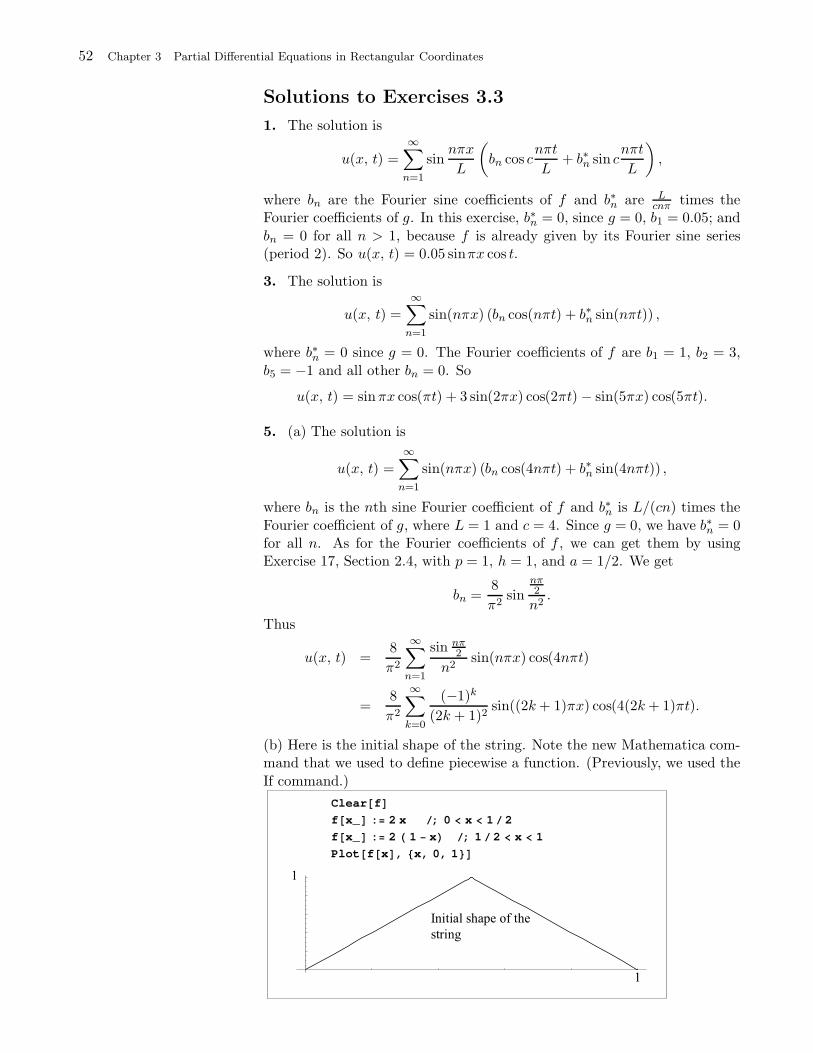
52 Chapter 3 Partial Differential Equations in Rectangular Coordinates
Solutions to Exercises 3.3
1. The solution is
u(x, t) =
∞∑
n=1
sinnπx
L
(bn cos c
nπt
L+ b∗n sin c
nπt
L
),
where bn are the Fourier sine coefficients of f and b∗n are Lcnπ times the
Fourier coefficients of g. In this exercise, b∗n = 0, since g = 0, b1 = 0.05; and
bn = 0 for all n > 1, because f is already given by its Fourier sine series(period 2). So u(x, t) = 0.05 sinπx cos t.
3. The solution is
u(x, t) =
∞∑
n=1
sin(nπx) (bn cos(nπt) + b∗n sin(nπt)) ,
where b∗n = 0 since g = 0. The Fourier coefficients of f are b1 = 1, b2 = 3,
b5 = −1 and all other bn = 0. So
u(x, t) = sinπx cos(πt) + 3 sin(2πx) cos(2πt) − sin(5πx) cos(5πt).
5. (a) The solution is
u(x, t) =
∞∑
n=1
sin(nπx) (bn cos(4nπt) + b∗n sin(4nπt)) ,
where bn is the nth sine Fourier coefficient of f and b∗n is L/(cn) times the
Fourier coefficient of g, where L = 1 and c = 4. Since g = 0, we have b∗n = 0for all n. As for the Fourier coefficients of f , we can get them by usingExercise 17, Section 2.4, with p = 1, h = 1, and a = 1/2. We get
bn =8
π2sin
nπ2
n2.
Thus
u(x, t) =8
π2
∞∑
n=1
sin nπ2
n2sin(nπx) cos(4nπt)
=8
π2
∞∑
k=0
(−1)k
(2k + 1)2sin((2k+ 1)πx) cos(4(2k+ 1)πt).
(b) Here is the initial shape of the string. Note the new Mathematica com-mand that we used to define piecewise a function. (Previously, we used the
If command.)
Clear f
f x_ : 2 x ; 0 x 1 2
f x_ : 2 1 x ; 1 2 x 1
Plot f x , x, 0, 1
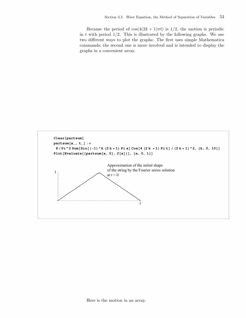
Section 3.3 Wave Equation, the Method of Separation of Variables 53
Because the period of cos(4(2k + 1)πt) is 1/2, the motion is periodicin t with period 1/2. This is illustrated by the following graphs. We usetwo different ways to plot the graphs: The first uses simple Mathematica
commands; the second one is more involved and is intended to display thegraphs in a convenient array.
Clear partsum
partsum x_, t_ :
8 Pi^2 Sum Sin 1 ^k 2 k 1 Pi x Cos 4 2 k 1 Pi t 2 k 1 ^2, k, 0, 10
Plot Evaluate partsum x, 0 , f x , x, 0, 1
Here is the motion in an array.
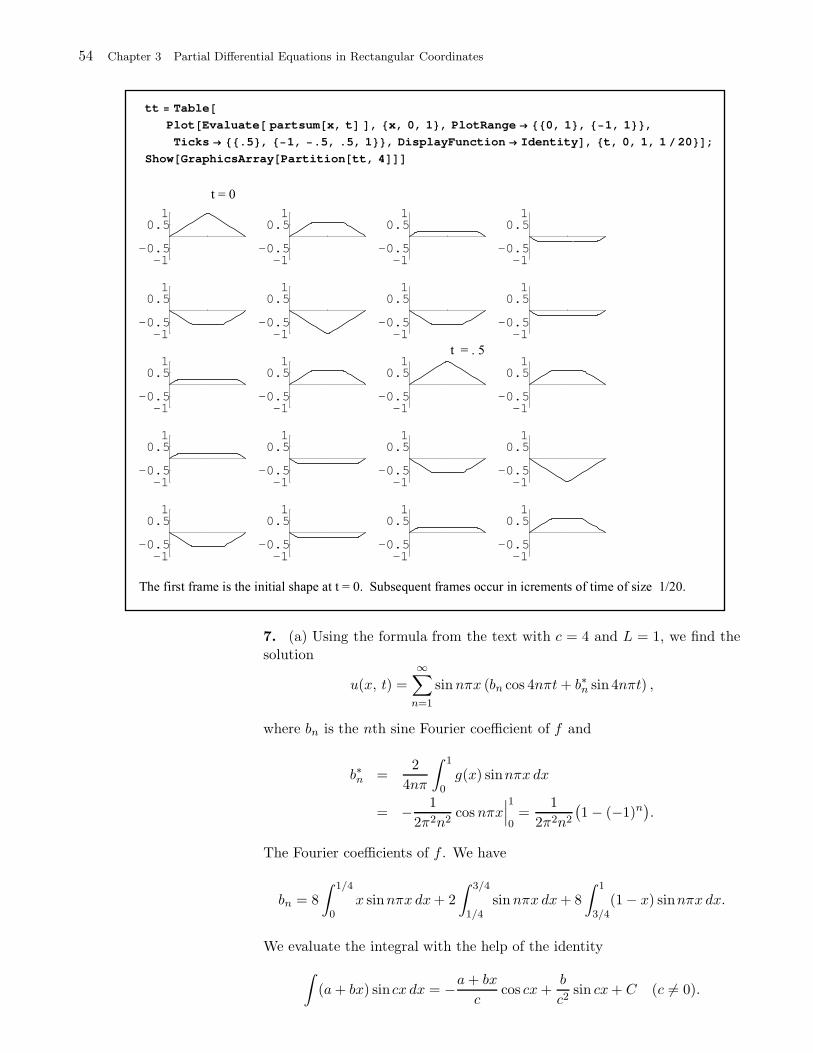
54 Chapter 3 Partial Differential Equations in Rectangular Coordinates
tt Table
Plot Evaluate partsum x, t , x, 0, 1 , PlotRange 0, 1 , 1, 1 ,
Ticks .5 , 1, .5, .5, 1 , DisplayFunction Identity , t, 0, 1, 1 20 ;
Show GraphicsArray Partition tt, 4
-1-0.5
0.51
-1-0.5
0.51
-1-0.5
0.51
-1-0.5
0.51
-1-0.5
0.51
-1-0.5
0.51
-1-0.5
0.51
-1-0.5
0.51
-1-0.5
0.51
-1-0.5
0.51
-1-0.5
0.51
-1-0.5
0.51
-1-0.5
0.51
-1-0.5
0.51
-1-0.5
0.51
-1-0.5
0.51
-1-0.5
0.51
-1-0.5
0.51
-1-0.5
0.51
-1-0.5
0.51
7. (a) Using the formula from the text with c = 4 and L = 1, we find the
solution
u(x, t) =
∞∑
n=1
sinnπx (bn cos 4nπt+ b∗n sin 4nπt) ,
where bn is the nth sine Fourier coefficient of f and
b∗n =2
4nπ
∫ 1
0g(x) sinnπx dx
= − 1
2π2n2cosnπx
∣∣∣1
0=
1
2π2n2
(1 − (−1)n
).
The Fourier coefficients of f . We have
bn = 8
∫ 1/4
0x sinnπx dx+ 2
∫ 3/4
1/4sinnπx dx+ 8
∫ 1
3/4(1− x) sinnπx dx.
We evaluate the integral with the help of the identity
∫(a+ bx) sincx dx = −a+ bx
ccos cx+
b
c2sin cx+ C (c 6= 0).
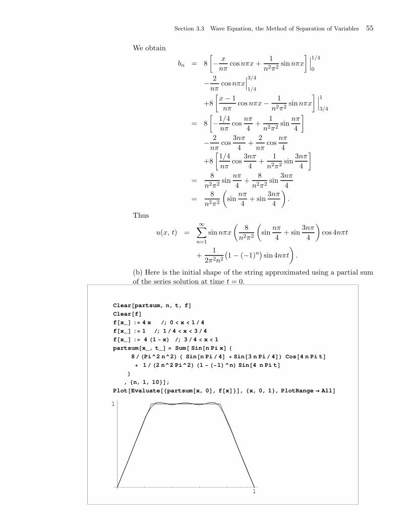
Section 3.3 Wave Equation, the Method of Separation of Variables 55
We obtain
bn = 8
[− x
nπcosnπx+
1
n2π2sinnπx
] ∣∣∣1/4
0
− 2
nπcosnπx
∣∣∣3/4
1/4
+8
[x− 1
nπcosnπx− 1
n2π2sinnπx
] ∣∣∣1
3/4
= 8
[−1/4
nπcos
nπ
4+
1
n2π2sin
nπ
4
]
− 2
nπcos
3nπ
4+
2
nπcos
nπ
4
+8
[1/4
nπcos
3nπ
4+
1
n2π2sin
3nπ
4
]
=8
n2π2sin
nπ
4+
8
n2π2sin
3nπ
4
=8
n2π2
(sin
nπ
4+ sin
3nπ
4
).
Thus
u(x, t) =∞∑
n=1
sinnπx
(8
n2π2
(sin
nπ
4+ sin
3nπ
4
)cos 4nπt
+1
2π2n2
(1 − (−1)n
)sin 4nπt
).
(b) Here is the initial shape of the string approximated using a partial sum
of the series solution at time t = 0.
Clear partsum, n, t, f
Clear f
f x_ : 4 x ; 0 x 1 4
f x_ : 1 ; 1 4 x 3 4
f x_ : 4 1 x ; 3 4 x 1
partsum x_, t_ Sum Sin n Pi x
8 Pi^2 n^2 Sin n Pi 4 Sin 3 n Pi 4 Cos 4 n Pi t
1 2 n^2 Pi^2 1 1 ^n Sin 4 n Pi t
, n, 1, 10 ;
Plot Evaluate partsum x, 0 , f x , x, 0, 1 , PlotRange All
1
1
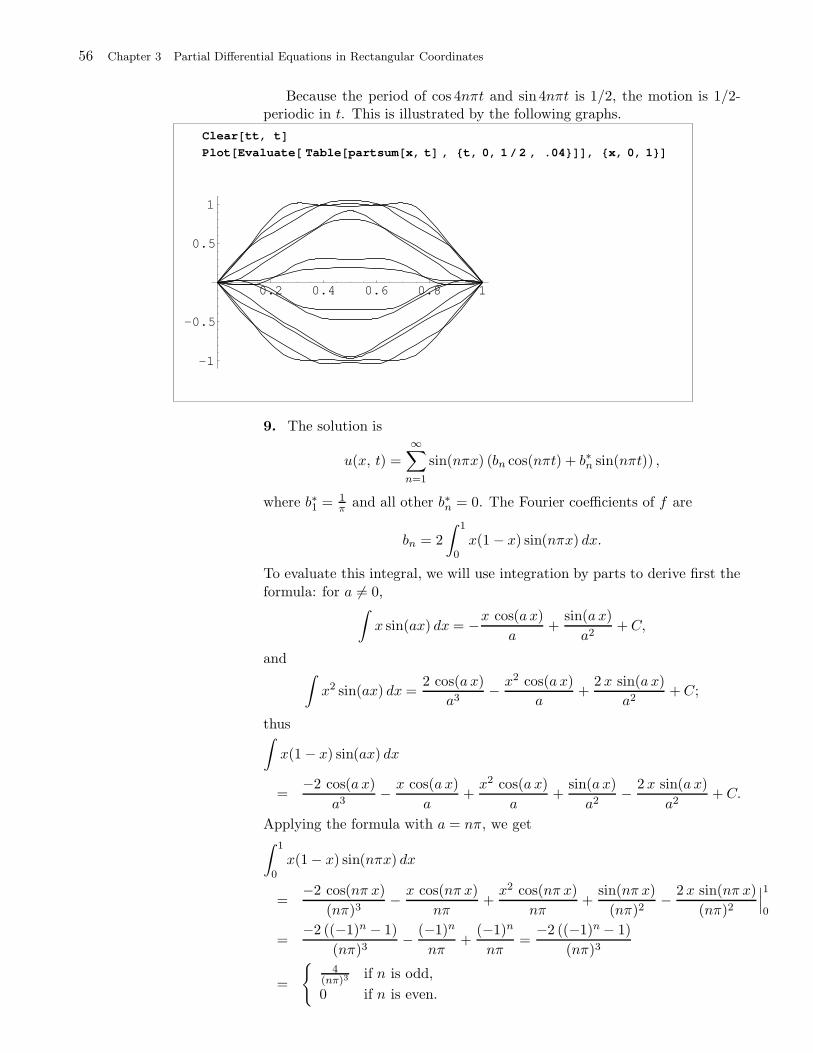
56 Chapter 3 Partial Differential Equations in Rectangular Coordinates
Because the period of cos 4nπt and sin 4nπt is 1/2, the motion is 1/2-periodic in t. This is illustrated by the following graphs.
Clear tt, t
Plot Evaluate Table partsum x, t , t, 0, 1 2 , .04 , x, 0, 1
0.2 0.4 0.6 0.8 1
-1
-0.5
0.5
1
9. The solution is
u(x, t) =
∞∑
n=1
sin(nπx) (bn cos(nπt) + b∗n sin(nπt)) ,
where b∗1 = 1π and all other b∗n = 0. The Fourier coefficients of f are
bn = 2
∫ 1
0x(1 − x) sin(nπx) dx.
To evaluate this integral, we will use integration by parts to derive first the
formula: for a 6= 0,∫x sin(ax) dx = −x cos(a x)
a+
sin(a x)
a2+C,
and∫x2 sin(ax) dx =
2 cos(a x)
a3− x2 cos(a x)
a+
2 x sin(a x)
a2+C;
thus∫x(1 − x) sin(ax) dx
=−2 cos(a x)
a3− x cos(a x)
a+x2 cos(a x)
a+
sin(a x)
a2− 2 x sin(a x)
a2+C.
Applying the formula with a = nπ, we get∫ 1
0
x(1− x) sin(nπx) dx
=−2 cos(nπ x)
(nπ)3− x cos(nπ x)
nπ+x2 cos(nπ x)
nπ+
sin(nπ x)
(nπ)2− 2 x sin(nπ x)
(nπ)2
∣∣∣1
0
=−2 ((−1)n − 1)
(nπ)3− (−1)n
nπ+
(−1)n
nπ=
−2 ((−1)n − 1)
(nπ)3
=
4
(nπ)3if n is odd,
0 if n is even.
Section 3.3 Wave Equation, the Method of Separation of Variables 57
Thus
bn =
8
(nπ)3if n is odd,
0 if n is even,
and so
u(x, t) =8
π3
∞∑
k=0
sin((2k+ 1)πx) cos((2k+ 1)πt)
(2k + 1)3+
1
πsin(πx) sin(πt).
11. (a) From (11),
un(x, t) = sinnπx
L
(bn cos
cnπt
L+ b∗n sin
cnπt
L
),
hence
un(x, t+2L
nc) = sin
nπx
L
(bn cos
cnπ(t+ 2Lnc )
L+ b∗n sin
cnπ(t+ 2Lnc )
L
)
= sinnπx
L
(bn cos(
cnπt
L+ 2π) + b∗n sin(
cnπt
L+ 2π)
)
= sinnπx
L
(bn cos
cnπt
L+ b∗n sin
cnπt
L
)= un(x, t),
so un(x, t) has time period 2Lnc . Since any positive integer multiple of a
period is also a period, we conclude that un(x, t) has time period 2Lc , and
since this period is independent of n, it follows that any linear combination
of un’s has period 2Lc . This applies to an infinite sum also. Hence the series
solution (8) is time periodic with period 2Lc , which proves (b). To prove (c),
note that
un(x, t+L
c) = sin
nπx
L
(bn cos
cnπ(t+ Lc )
L+ b∗n sin
cnπ(t+ Lc )
L
)
= sinnπx
L
(bn cos(
cnπt
L+ nπ) + b∗n sin(
cnπt
L+ nπ)
)
= (−1)n sinnπx
L
(bn cos
cnπt
L+ b∗n sin
cnπt
L
)
= sin(nπx
L− nπ)
(bn cos
cnπt
L+ b∗n sin
cnπt
L
)
= − sin(nπ(L− x)
L)
(bn cos
cnπt
L+ b∗n sin
cnπt
L
)
= −un(L− x, t).
Since this relation holds for every n, summing over n, we obtain
u(x, t+L
c) =
∞∑
n=1
u(x, t+L
c) = −
∞∑
n=1
u(L− x, t) = −u(L− x, t).
Think of the string at time t as part of an odd 2L-periodic graph, so that we
can talk about u(x, t) for x outside the interval [0, L]. Moreover, we haveu(−x, t) = −u(x, t) and u(x+2L, t) = u(x, t). This graph moves as t variesand returns to its original shape at t+ 2L
c . The shape of the string at time
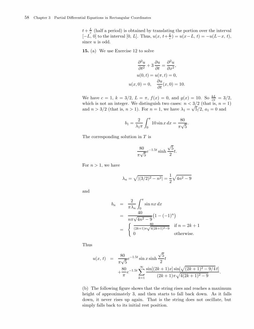
58 Chapter 3 Partial Differential Equations in Rectangular Coordinates
t+ Lc (half a period) is obtained by translating the portion over the interval
[−L, 0] to the interval [0, L]. Thus, u(x, t+ Lc ) = u(x−L, t) = −u(L−x, t),
since u is odd.
15. (a) We use Exercise 12 to solve
∂2u
∂t2+ 3
∂u
∂t=∂2u
∂x2,
u(0, t) = u(π, t) = 0,
u(x, 0) = 0,∂u
∂t(x, 0) = 10.
We have c = 1, k = 3/2, L = π, f(x) = 0, and g(x) = 10. So kLcπ = 3/2,
which is not an integer. We distinguish two cases: n < 3/2 (that is, n = 1)
and n > 3/2 (that is, n > 1). For n = 1, we have λ1 =√
5/2, a1 = 0 and
b1 =2
λ1π
∫ π
010 sinx dx =
80
π√
5.
The corresponding solution in T is
80
π√
5e−1.5t sinh
√5
2t.
For n > 1, we have
λn =√|(3/2)2 − n2| =
1
2
√4n2 − 9
and
bn =2
πλn
∫ π
0sinnx dx
=40
nπ√
4n2 − 9
(1 − (−1)n
)
=
80
(2k+1)π√
4(2k+1)2−9if n = 2k + 1
0 otherwise.
Thus
u(x, t) =80
π√
5e−1.5t sinx sinh
√5
2t
+80
πe−1.5t
∞∑
k=1
sin[(2k+ 1)x] sin[√
(2k + 1)2 − 9/4 t]
(2k+ 1)π√
4(2k+ 1)2 − 9.
(b) The following figure shows that the string rises and reaches a maximumheight of approximately 3, and then starts to fall back down. As it falls
down, it never rises up again. That is the string does not oscillate, butsimply falls back to its initial rest position.
Section 3.3 Wave Equation, the Method of Separation of Variables 59
u x_, t_ 80 Pi Sqrt 5 E^ 3 2 t Sin x Sinh Sqrt 5 2 t
40 Pi E^ 3 2 t Sum Sin 2 j 1 x
Sin Sqrt 2 j 1 ^2 9 4 t 2 j 1 Sqrt 2 j 1 ^2 9 4 , j, 1, 7 ;
tt Table u x, t , t, .1, 8, .6 ;
Plot Evaluate tt , x, 0, Pi , PlotRange All
0.5 1 1.5 2 2.5 3
0.5
1
1.5
2
2.5
3
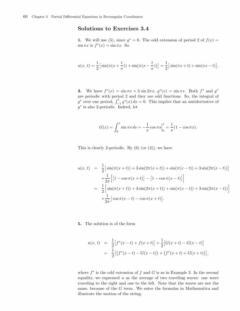
60 Chapter 3 Partial Differential Equations in Rectangular Coordinates
Solutions to Exercises 3.4
1. We will use (5), since g∗ = 0. The odd extension of period 2 of f(x) =sinπx is f∗(x) = sinπx. So
u(x, t) =1
2
[sin(π(x+
t
π)) + sin(π(x− t
π))]
=1
2
[sin(πx+ t) + sin(πx− t)
].
3. We have f∗(x) = sinπx + 3 sin 2πx, g∗(x) = sinπx. Both f∗ and g∗
are periodic with period 2 and they are odd functions. So, the integral of
g∗ over one period,∫ 1−1 g
∗(x) dx = 0. This implies that an antiderivative ofg∗ is also 2-periodic. Indeed, let
G(x) =
∫ x
0
sinπs ds = −1
πcos πs
∣∣∣x
0=
1
π(1− cosπx).
This is clearly 2-periodic. By (6) (or (4)), we have
u(x, t) =1
2
[sin(π(x+ t)) + 3 sin(2π(x+ t)) + sin(π(x− t)) + 3 sin(2π(x− t))
]
+1
2π
[[1 − cos π(x+ t)
]−[1 − cos π(x− t)
]]
=1
2
[sin(π(x+ t)) + 3 sin(2π(x+ t)) + sin(π(x− t)) + 3 sin(2π(x− t))
]
+1
2π
[cosπ(x− t) − cosπ(x+ t)
].
5. The solution is of the form
u(x, t) =1
2
[f∗(x− t) + f(x+ t)
]+
1
2
[G(x+ t) −G(x− t)
]
=1
2
[(f∗(x− t) −G(x− t)
)+(f∗(x+ t) +G(x+ t)
)],
where f∗ is the odd extension of f and G is as in Example 3. In the secondequality, we expressed u as the average of two traveling waves: one wave
traveling to the right and one to the left. Note that the waves are not thesame, because of the G term. We enter the formulas in Mathematica andillustrate the motion of the string.
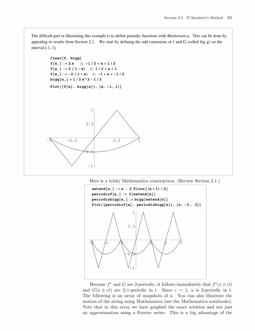
Section 3.4 D’Alembert’s Method 61
The difficult part in illustrating this example is to define periodic functions with Mathematica. This can be done by
appealing to results from Section 2.1. We start by defining the odd extensions of f and G (called big g) on the
interval [-1, 1].
Clear f, bigg
f x_ : 2 x ; 1 2 x 1 2
f x_ : 2 1 x ; 1 2 x 1
f x_ : 2 1 x ; 1 x 1 2
bigg x_ 1 2 x^2 1 2
Plot f x , bigg x , x, 1, 1
-1 -0.5 0.5 1
-1
-0.5
0.5
1
Here is a tricky Mathematica construction. (Review Section 2.1.)
extend x_ : x 2 Floor x 1 2
periodicf x_ : f extend x
periodicbigg x_ : bigg extend x
Plot periodicf x , periodicbigg x , x, 3 , 3
-3 -2 -1 1 2 3
-1
-0.5
0.5
1
Because f∗ and G are 2-periodic, it follows immediately that f∗(x± ct)
and G(x ± ct) are 2/c-periodic in t. Since c = 1, u is 2-periodic in t.The following is an array of snapshots of u. You can also illustrate the
motion of the string using Mathematica (see the Mathematica notebooks).Note that in this array we have graphed the exact solution and not justan approximation using a Fourier series. This is a big advantage of the
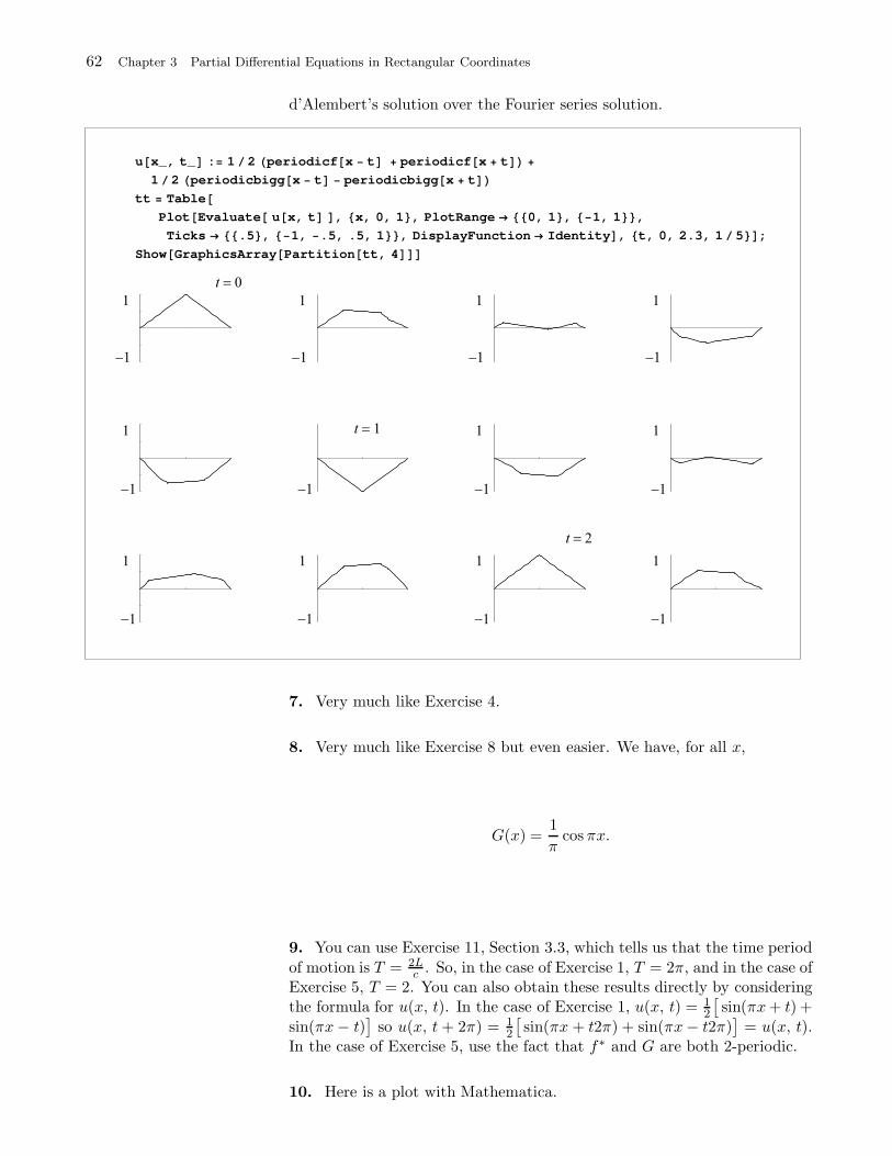
62 Chapter 3 Partial Differential Equations in Rectangular Coordinates
d’Alembert’s solution over the Fourier series solution.
u x_, t_ : 1 2 periodicf x t periodicf x t
1 2 periodicbigg x t periodicbigg x t
tt Table
Plot Evaluate u x, t , x, 0, 1 , PlotRange 0, 1 , 1, 1 ,
Ticks .5 , 1, .5, .5, 1 , DisplayFunction Identity , t, 0, 2.3, 1 5 ;
Show GraphicsArray Partition tt, 4
7. Very much like Exercise 4.
8. Very much like Exercise 8 but even easier. We have, for all x,
G(x) =1
πcos πx.
9. You can use Exercise 11, Section 3.3, which tells us that the time period
of motion is T = 2Lc . So, in the case of Exercise 1, T = 2π, and in the case of
Exercise 5, T = 2. You can also obtain these results directly by consideringthe formula for u(x, t). In the case of Exercise 1, u(x, t) = 1
2
[sin(πx+ t) +
sin(πx− t)]
so u(x, t+ 2π) = 12
[sin(πx + t2π) + sin(πx− t2π)
]= u(x, t).
In the case of Exercise 5, use the fact that f∗ and G are both 2-periodic.
10. Here is a plot with Mathematica.
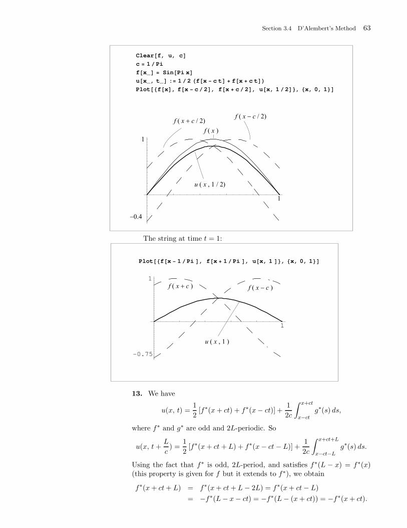
Section 3.4 D’Alembert’s Method 63
Clear f, u, c
c 1 Pi
f x_ Sin Pi x
u x_, t_ : 1 2 f x c t f x c t
Plot f x , f x c 2 , f x c 2 , u x, 1 2 , x, 0, 1
The string at time t = 1:
Plot f x 1 Pi , f x 1 Pi , u x, 1 , x, 0, 1
1
-0.75
1
13. We have
u(x, t) =1
2[f∗(x+ ct) + f∗(x− ct)] +
1
2c
∫ x+ct
x−ctg∗(s) ds,
where f∗ and g∗ are odd and 2L-periodic. So
u(x, t+L
c) =
1
2[f∗(x+ ct+ L) + f∗(x− ct− L)] +
1
2c
∫ x+ct+L
x−ct−Lg∗(s) ds.
Using the fact that f∗ is odd, 2L-period, and satisfies f∗(L − x) = f∗(x)(this property is given for f but it extends to f∗), we obtain
f∗(x+ ct+ L) = f∗(x+ ct+ L− 2L) = f∗(x+ ct− L)
= −f∗(L− x− ct) = −f∗(L− (x+ ct)) = −f∗(x+ ct).
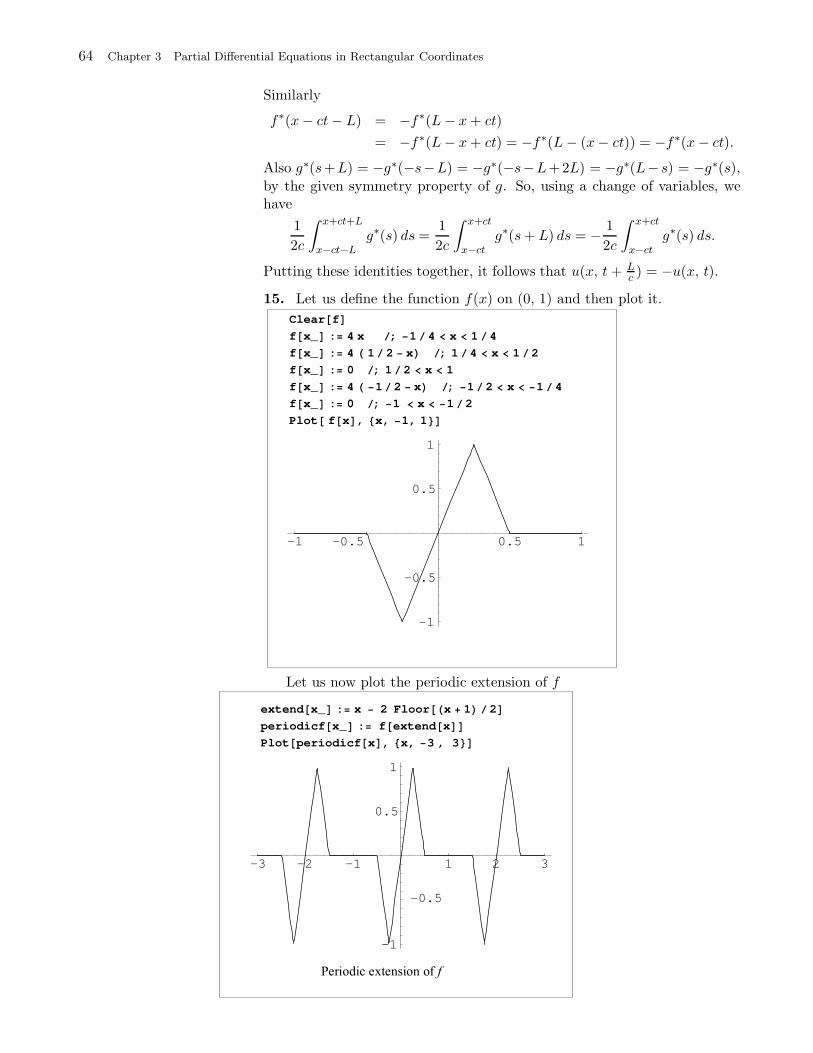
64 Chapter 3 Partial Differential Equations in Rectangular Coordinates
Similarly
f∗(x− ct− L) = −f∗(L− x+ ct)
= −f∗(L− x+ ct) = −f∗(L− (x− ct)) = −f∗(x− ct).
Also g∗(s+L) = −g∗(−s−L) = −g∗(−s−L+2L) = −g∗(L− s) = −g∗(s),by the given symmetry property of g. So, using a change of variables, wehave
1
2c
∫ x+ct+L
x−ct−Lg∗(s) ds =
1
2c
∫ x+ct
x−ctg∗(s+ L) ds = − 1
2c
∫ x+ct
x−ctg∗(s) ds.
Putting these identities together, it follows that u(x, t+ Lc ) = −u(x, t).
15. Let us define the function f(x) on (0, 1) and then plot it.
Clear f
f x_ : 4 x ; 1 4 x 1 4
f x_ : 4 1 2 x ; 1 4 x 1 2
f x_ : 0 ; 1 2 x 1
f x_ : 4 1 2 x ; 1 2 x 1 4
f x_ : 0 ; 1 x 1 2
Plot f x , x, 1, 1
-1 -0.5 0.5 1
-1
-0.5
0.5
1
Let us now plot the periodic extension of f
extend x_ : x 2 Floor x 1 2
periodicf x_ : f extend x
Plot periodicf x , x, 3 , 3
-3 -2 -1 1 2 3
-1
-0.5
0.5
1
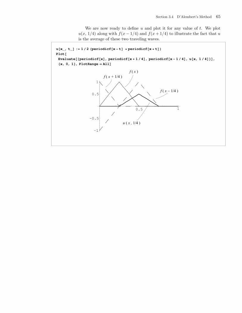
Section 3.4 D’Alembert’s Method 65
We are now ready to define u and plot it for any value of t. We plotu(x, 1/4) along with f(x− 1/4) and f(x+ 1/4) to illustrate the fact that u
is the average of these two traveling waves.
u x_, t_ : 1 2 periodicf x t periodicf x t
Plot
Evaluate periodicf x , periodicf x 1 4 , periodicf x 1 4 , u x, 1 4 ,
x, 0, 1 , PlotRange All
0.5 1
-1
-0.5
0.5
1
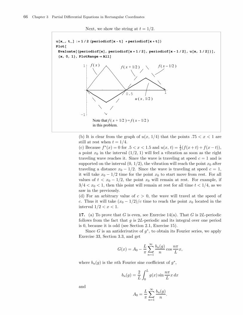
66 Chapter 3 Partial Differential Equations in Rectangular Coordinates
Next, we show the string at t = 1/2.
u x_, t_ : 1 2 periodicf x t periodicf x t
Plot
Evaluate periodicf x , periodicf x 1 2 , periodicf x 1 2 , u x, 1 2 ,
x, 0, 1 , PlotRange All
0.5 1
-1
1
(b) It is clear from the graph of u(x, 1/4) that the points .75 < x < 1 arestill at rest when t = 1/4.
(c) Because f∗(x) = 0 for .5 < x < 1.5 and u(x, t) = 12 (f(x+ t) + f(x− t)),
a point x0 in the interval (1/2, 1) will feel a vibration as soon as the right
traveling wave reaches it. Since the wave is traveling at speed c = 1 and issupported on the interval (0, 1/2), the vibration will reach the point x0 after
traveling a distance x0 − 1/2. Since the wave is traveling at speed c = 1,it will take x0 − 1/2 time for the point x0 to start move from rest. For allvalues of t < x0 − 1/2, the point x0 will remain at rest. For example, if
3/4 < x0 < 1, then this point will remain at rest for all time t < 1/4, as wesaw in the previously.
(d) For an arbitrary value of c > 0, the wave will travel at the speed ofc. Thus it will take (x0 − 1/2)/c time to reach the point x0 located in the
interval 1/2 < x < 1.
17. (a) To prove that G is even, see Exercise 14(a). That G is 2L-periodic
follows from the fact that g is 2L-periodic and its integral over one periodis 0, because it is odd (see Section 2.1, Exercise 15).
Since G is an antiderivative of g∗, to obtain its Fourier series, we applyExercise 33, Section 3.3, and get
G(x) = A0 −L
π
∞∑
n=1
bn(g)
ncos
nπ
Lx,
where bn(g) is the nth Fourier sine coefficient of g∗,
bn(g) =2
L
∫ L
0g(x) sin
nπ
Lx dx
and
A0 =L
π
∞∑
n=1
bn(g)
n.
Section 3.4 D’Alembert’s Method 67
In terms of b∗n, we have
L
π
bn(g)
n=
2
nπ
∫ L
0g(x) sin
nπ
Lx dx = cb∗n,
and so
G(x) =L
π
∞∑
n=1
bn(g)
n− L
π
∞∑
n=1
bn(g)
ncos
nπ
Lx
=
∞∑
n=1
cb∗n
(1 − cos(
nπ
Lx)).
(b) From (a), it follows that
G(x+ ct) −G(x− ct) =
∞∑
n=1
cb∗n
[(1 − cos(
nπ
L(x+ ct))
)−(1 − cos(
nπ
L(x− ct))
)]
=
∞∑
n=1
−cb∗n[cos(
nπ
L(x+ ct)) − cos(
nπ
L(x− ct))
]
(c) Continuing from (b) and using the notation in the text, we obtain
1
2c
∫ x+ct
x−ctg∗(s) ds =
1
2c[G(x+ ct) −G(x− ct)]
=
∞∑
n=1
−b∗n1
2
[cos(
nπ
L(x+ ct)) − cos(
nπ
L(x− ct))
]
=
∞∑
n=1
b∗n sin(nπ
Lx) sin(
nπ
Lct)
=
∞∑
n=1
b∗n sin(nπ
Lx) sin(λnt).
(d) To derive d’Alembert’s solution from (8), Section 3.3, proceed as follows:
u(x, t) =
∞∑
n=1
bn sin(nπ
Lx) cos(λnt) +
∞∑
n=1
b∗n sin(nπ
Lx) sin(λnt)
=1
2
(f∗(x− ct) + f∗(x+ ct)
)+
1
2c[G(x+ ct) −G(x− ct)] ,
where in the last equality we used Exercise 16 and part (c).
19. (a) The characteristic lines are lines with slope ±1/c = ±1 in the
xt-plane.(b) The interval of dependence of a point (x0, t0) is the interval on the x-
axis, centered at x0, with radius ct0. For the point (.5, .2) this interval is.3 ≤ x ≤ .7. For the point (.3, 2) this interval is −1.8 ≤ x ≤ 2.3.
(c) The horizontal, semi-infinite, strip S is bounded by the line x = 0 andx = 1 and lies in the upper half-plane. The region I is the triangular
region with base on the interval (0, 1), bounded by the lines through (0, 0)at slope 1, and through (1, 0) at slope −1. The three vertices of I are (0, 0),(1/2, 1/2), and (0, 1). The point (.5, .2) is in I but the point (.3, 2) is not
68 Chapter 3 Partial Differential Equations in Rectangular Coordinates
in I .(d) For the points (x, t) in I , u(x, t) depends only on f and g and not theirperiodic extension. We have
u(x, t) = =1
2
[f(x− t) + f(x+ t)
]+
1
2
∫ x+t
x−tg(s) ds
=1
2
∫ x+t
x−t
s ds
=1
4s2∣∣∣x+t
x−t=
1
4
[(x+ t)2 − (x− t)2
]= xt.
21. Follow the labeling of Figure 8 in Section 3.4. Let P1 = (x0, t0) be anarbitrary point in the region II . Form a characteristic parallelogram with
vertices P1, P2, Q1, Q2, as shown in Figure 8 in Section 3.4. The verticesP2 and Q1 are on the characteristic line x+ 2t = 1 and the vertex Q2 is on
the boundary line x = 1. From Proposition 1, we have
u(P1) = u(Q1) + u(Q2) − u(P2) = u(Q1) − u(P2),
because u(Q2) = 0. We will find u(P2) and u(Q1) by using the formula
u(x, t) = −4t2 + x − x2 + 8tx from Example 4, because P2 and Q1 are inthe region I .
The point Q1 is the intersection point of the characteristic lines x−2t =x0 − 2t0 and x + 2t = 1. Adding the equations and then solving for x, we
get
x =x0 + 1 − 2t0
2.
The second coordinate of Q1 is then
t =1 − x0 + 2t0
4.
The point Q2 is the intersection point of the characteristic line x+ 2t =x0 + 2t0 and x = 1. Thus
t =x0 + 2t0 − 1
2.
The point P2 is the intersection point of the characteristic lines x+2t = 1
and x− 2t = 1− (x0 + 2t0 − 1). Solving for x and t, we find the coordinatesof P2 to be
x =3− x0 − 2t0
2and t =
−1 + x0 + 2t04
.
To simplify the notation, replace x0 and t0 by x and y in the coordinates ofthe points Q1 and P2 and let φ(x, t) = −4t2 + x− x2 + 8tx. We have
u(x, t) = u(Q1) − u(P2)
= φ
(x+ 1 − 2t
2,
1− x+ 2t
4
)− φ
(3− x− 2t
2,−1 + x+ 2t
4
)
= 5 − 12t− 5x+ 12tx,
where the last expression was derived after a few simplifications that weomit. It is interesting to note that the formula satisfies the wave equation
and the boundary condition u(1, t) = 0 for all t > 0. Its restriction to theline x+2t = 1 (part of the boundary of region I) reduces to the formula for
u(x, t) for (x, t) in region I . This is to be expected since u is continuous in(x, t).
Section 3.5 The One Dimensional Heat Equation 69
Solutions to Exercises 3.5
1. Multiply the solution in Example 1 by 78100 to obtain
u(x, t) =312
π
∞∑
k=0
e−(2k+1)2t
2k + 1sin(2k + 1)x.
3. We have
u(x, t) =
∞∑
n=1
bne−n2t sin(nx),
where
bn =66
π
∫ π/2
0x sinnx dx+
66
π
∫ π
π/2(π − x) sinnx dx
=66
π
(−x cos(nx)
n+
sin(nx)
n2
) ∣∣∣π/2
0
+66
π
(−(π − x) cos(nx)
n− sin(nx)
n2
) ∣∣∣π
π/2
=66
π
(−
π2 cos(nπ
2 )
n+
sin(nπ2 )
n2+
π2 cos(nπ
2 )
n+
sin(nπ2 )
n2
)
=132
π
sin(nπ2 )
n2
=
132 (−1)k
π(2k+1)2if n = 2k + 1,
0 if n = 2k.
Thus
u(x, t) =132
π
∞∑
k=0
e−(2k+1)2t sin((2k+ 1)x)
(2k+ 1)2.
5. We have
u(x, t) =
∞∑
n=1
bne−(nπ)2t sin(nπx),
where
bn = 2
∫ 1
0x sin(nπx) dx = 2
[−x cos(nπ x)
nπ+
sin(nπ x)
n2 π2
] ∣∣∣1
0
= −2cosnπ
nπ= 2
(−1)n+1
nπ.
So
u(x, t) =2
π
∞∑
n=1
(−1)n+1e−(nπ)2t sin(nπx)
n.
7. (a) From the figures in Example 1, we can see that when t is equal to 1
the temperature is already below 50 degrees. We will give a more accurateapproximation. Let us first check the solution by plotting an approximationof the initial temperature distribution.
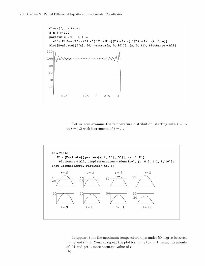
70 Chapter 3 Partial Differential Equations in Rectangular Coordinates
Clear f, partsum
f x_ : 100
partsum x_, t_, n_ :
400 Pi Sum E^ 2 k 1 ^2 t Sin 2 k 1 x 2 k 1 , k, 0, n ;
Plot Evaluate f x , 50, partsum x, 0, 20 , x, 0, Pi , PlotRange All
0.5 1 1.5 2 2.5 3
20
40
60
80
100
120
Let us now examine the temperature distribution, starting with t = .5
to t = 1.2 with increments of t = .1.
tt Table
Plot Evaluate partsum x, t, 10 , 50 , x, 0, Pi ,
PlotRange All, DisplayFunction Identity , t, 0.5, 1.2, 1 10 ;
Show GraphicsArray Partition tt, 4
50 50 50
30
50
4060
4060 50
50
It appears that the maximum temperature dips under 50 degree between
t = .9 and t = 1. You can repeat the plot for t = .9 to t = 1, using incrementsof .01 and get a more accurate value of t.(b)
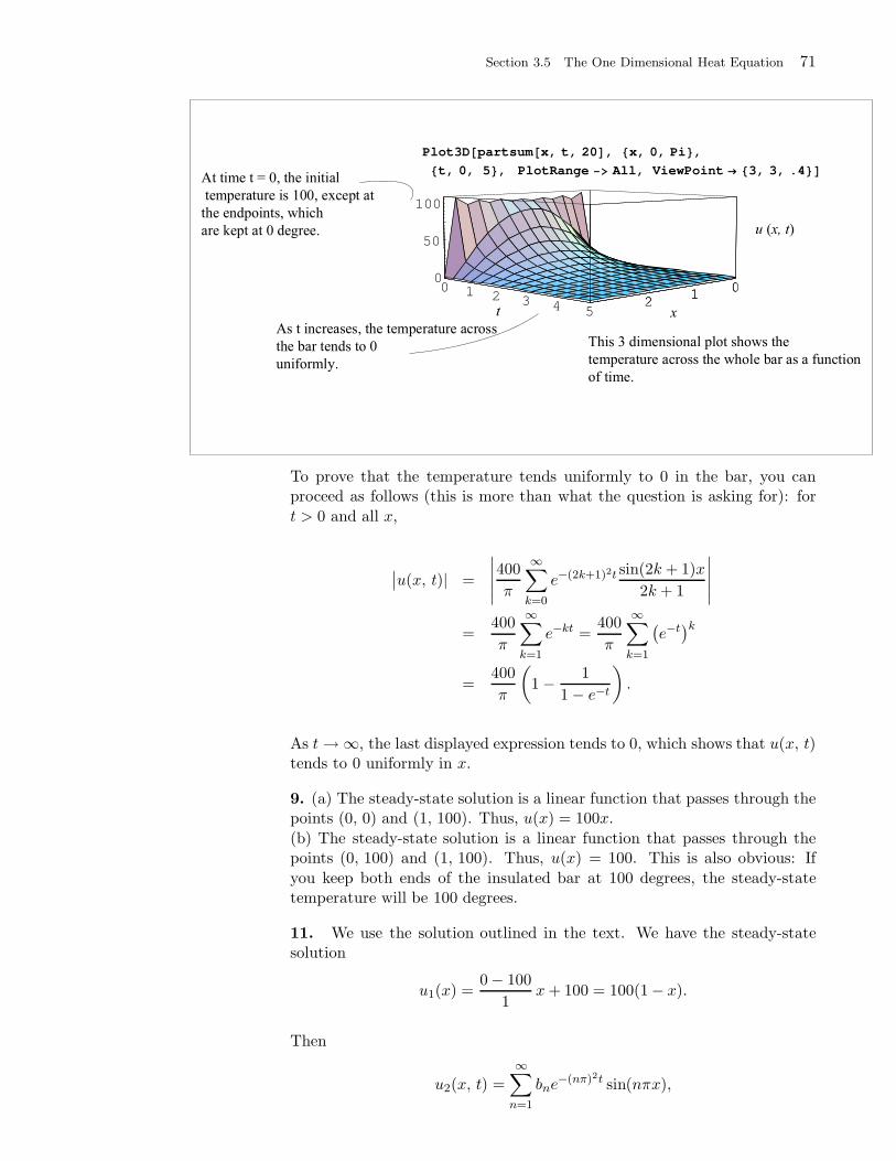
Section 3.5 The One Dimensional Heat Equation 71
Plot3D partsum x, t, 20 , x, 0, Pi ,
t, 0, 5 , PlotRange All, ViewPoint 3, 3, .4
01
20 1 2 3 4 5
0
50
100
01
2
To prove that the temperature tends uniformly to 0 in the bar, you canproceed as follows (this is more than what the question is asking for): for
t > 0 and all x,
∣∣u(x, t)| =
∣∣∣∣∣400
π
∞∑
k=0
e−(2k+1)2t sin(2k + 1)x
2k + 1
∣∣∣∣∣
=400
π
∞∑
k=1
e−kt =400
π
∞∑
k=1
(e−t)k
=400
π
(1 − 1
1 − e−t
).
As t→ ∞, the last displayed expression tends to 0, which shows that u(x, t)tends to 0 uniformly in x.
9. (a) The steady-state solution is a linear function that passes through thepoints (0, 0) and (1, 100). Thus, u(x) = 100x.
(b) The steady-state solution is a linear function that passes through thepoints (0, 100) and (1, 100). Thus, u(x) = 100. This is also obvious: If
you keep both ends of the insulated bar at 100 degrees, the steady-statetemperature will be 100 degrees.
11. We use the solution outlined in the text. We have the steady-statesolution
u1(x) =0− 100
1x+ 100 = 100(1− x).
Then
u2(x, t) =
∞∑
n=1
bne−(nπ)2t sin(nπx),
72 Chapter 3 Partial Differential Equations in Rectangular Coordinates
where
bn = 2
∫ 1
0
(30 sin(πx)− 100(1− x)
)sin(nπx) dx
=
=30 if n=1, 0 if n6=1︷ ︸︸ ︷
60
∫ 1
0sin(πx) sin(nπx) dx−
= 200nπ︷ ︸︸ ︷
200
∫ 1
0(1 − x) sin(nπx) dx
=
30 − 200
π if n = 1,
−200nπ if n > 1.
Thus So
u(x, t) = u1(x)+u2(x, t) = 100(1−x)+30 e−π2t sinπx−200
π
∞∑
n=1
e−(nπ)2t sin(nπx)
n.
13. We have u1(x) = −50π x + 100. We use (13) and the formula from
Exercise 10, and get (recall the Fourier coefficients of f from Exercise 3)
u(x, t) = −50
πx + 100
+∞∑
n=1
[132
π
sin(nπ2 )
n2− 100
(2 − (−1)n
nπ
)]e−n2t sinnx.
15. From (14), we have bn = 0, since f(x)− u1(x) = 0. Hence u2(x, t) = 0
and so u(x, t) = u1(x) = steady-state solution. This is obvious on physicalgrounds: If the initial temperature distribution is already in equilibrium,
then it will not change.
17. Fix t0 > 0 and consider the solution at time t = t0:
u(x, t0) =
∞∑
n=1
bn sinnπ
Lxe−λ2
nt0.
We will show that this series converges uniformly for all x (not just 0 ≤ x ≤L) by appealing to the Weierstrass M -test. For this purpose, it suffices to
establish the following two inequalities:(a)
∣∣bn sin nπL xe
−λ2nt0∣∣ ≤Mn for all x; and
(b)∑∞
n=1 Mn <∞.To establish (a), note that
|bn| =
∣∣∣∣2
L
∫ L
0f(x) sin
nπ
Lx dx
∣∣∣∣ ≤2
L
∫ L
0
∣∣∣f(x) sinnπ
Lx∣∣∣ dx
(The absolute value of the integral is
≤ the integral of the absolute value.)
≤ 2
L
∫ L
0
|f(x)| dx = A (because | sinu| ≤ 1 for all u).
Note that A is a finite number because f is bounded, so its absolute valueis bounded and hence its integral is finite on [0, L]. We have
∣∣bn sinnπ
Lxe−λ2
nt0∣∣ ≤ Ae−λ2
nt0 = Ae−c2π2t0
L2 n2
≤ A
(e−
c2π2t0L2
)n
= Arn,
Section 3.5 The One Dimensional Heat Equation 73
where r = e−c2π2t0
L2 < 1. Take Mn = Arn. Then a holds and∑Mn is
convergent because it is a geometric series with ratio r < 1.
74 Chapter 3 Partial Differential Equations in Rectangular Coordinates
Solutions to Exercises 3.6
1. Since the bar is insulated and the temperature inside is constant, there isno exchange of heat, and so the temperature remains constant for all t > 0.
Thus u(x, t) = 100 for all t > 0. This is also a consequence of (2), since inthis case all the an’s are 0 except a0 = 100.
3. We apply (4):
u(x, t) = a0 +∞∑
n=1
ane−n2t cosnx,
where
a0 =1
π
∫ π/2
0100 x dx+
1
π
∫ π/2
0100 (π− x) dx
=50
πx2∣∣∣π/2
0− 50
π(π − x)2
∣∣∣π
π/2=
25
2π +
25
2π = 25π,
and
an =2
π
∫ π/2
0
100 x cosnx dx+2
π
∫ π/2
0
100 (π− x) cosnx dx
=200
π
(cosnx
n2+x sinnx
n
) ∣∣∣π/2
0
+200
π
(−cosnx
n2+
(π − x) sinnx
n
) ∣∣∣π
π/2
=200
π
(cosn π
2
n2+
π2 sinn π
2
n+
cosn π2
n2−
π2 sinn π
2
n− 1
n2− cosnπ
n2
)
=200
πn2
(2 cosn
π
2− (1 + (−1)n)
)
=
0 if n = 4k + 1 or n = 4k + 3,0 if n = 4k or n = 4k + 3,
− 800πn2 if n = 4k + 2 = 2(2k+ 1).
So
u(x, t) = 25π − 200
π
∞∑
k=0
1
(2k + 1)2e−4(2k+1)2t cos(2(2k+ 1)x),
5. Apply the separation of variables method as in Example 1; you willarrive at the following equations in X and T :
X ′′ − kX = 0, X(0) = 0, X ′(L) = 0
T ′ − kc2T = 0 .
We now show that the separation constant k has to be negative by rulingout the possibilities k = 0 and k > 0.
If k = 0 then X ′′ = 0 ⇒ X = ax+b. Use the initial conditions X(0) = 0implies that b = 0, X ′(L) = 0 implies that a = 0. So X = 0 if k = 0.
Section 3.6 Heat Conduction in Bars: Varying the Boundary Conditions 75
If k > 0, say k = µ2, where µ > 0, then
X ′′ − µ2X = 0 ⇒ X = c1 coshµx + c2 sinhµx;
X(0) = 0 ⇒ 0 = c1;X = c2 sinhµx;
X ′(L) = 0 ⇒ 0 = c2µ cosh(µL)
⇒ c2 = 0,
because µ 6= 0 and cosh(µL) 6= 0. So X = 0 if k > 0. This leaves the casek = −µ2, where µ > 0. In this case
X ′′ + µ2X = 0 ⇒ X = c1 cosµx + c2 sinµx;
X(0) = 0 ⇒ 0 = c1;X = c2 sinµx;
X ′(L) = 0 ⇒ 0 = c2µ cos(µL)
⇒ c2 = 0 or cos(µL) = 0.
To avoid the trivial solution, we set cos(µL) = 0, which implies that
µ = (2k + 1)π
2L, k = 0, 1, . . . .
Plugging this value of k in the equation for T , we find
T ′ + µ2c2T = 0 ⇒ T (t) = Bke−µ2c2t = Bke
−((2k+1) π2L)
2c2t.
Forming the product solutions and superposing them, we find that
u(x, t) =
∞∑
k=0
Bke−µ2c2t =
∞∑
k=0
Bke−((2k+1) π
2L)2c2t sin
[(2k + 1)
π
2Lx].
To determine the coefficients Bk, we use the initial condition and proceedas in Example 1:
u(x, 0) = f(x) ⇒ f(x) =
∞∑
k=0
Bk sin[(2k+ 1)
π
2Lx];
⇒ f(x) sin[(2n+ 1)
π
2Lx]
=
∞∑
k=0
Bk sin[(2k+ 1)
π
2Lx]sin[(2n+ 1)
π
2Lx]
⇒∫ L
0f(x) sin
[(2n+ 1)
π
2Lx]dx
=
∞∑
k=0
Bk
∫ L
0sin[(2k+ 1)
π
2Lx]sin[(2n+ 1)
π
2Lx]dx
⇒∫ L
0
f(x) sin[(2n+ 1)
π
2Lx]dx
= Bn
∫ L
0sin2
[(2n+ 1)
π
2Lx]dx,
76 Chapter 3 Partial Differential Equations in Rectangular Coordinates
where we have integrated the series term by term and used the orthogonalityof the functions sin
[(2k+ 1) π
2Lx]
on the interval [0, L]. The orthogonality
can be checked directly by verifying that
∫ L
0
sin[(2k + 1)
π
2Lx]sin[(2n+ 1)
π
2Lx]dx = 0
if n 6= k. Solving for Bn and using that
∫ L
0sin2
[(2n+ 1)
π
2Lx]dx =
L
2
(check this using a half-angle formula), we find that
Bn =2
L
∫ L
0f(x) sin
[(2n+ 1)
π
2Lx]dx.
7. In the first part of this solution, we will justify term-by-term integrationof the series solution. Recall that the solution is given by
u(x, t) = a0 +
∞∑
n=1
ane−λ2
nt cosnπx
L,
where an is the cosine Fourier coefficient of f . Since f is a temperature
distribution, we can suppose that it is bounded; hence |f(x)| ≤M for all x,where M is a constant. Hence
|an| =2
L
∣∣∣∣∫ L
0
f(x) cosnπ
Ldx
∣∣∣∣ ≤2
L
∫ L
0
≤M︷ ︸︸ ︷|f(x)|
≤1︷ ︸︸ ︷∣∣∣cosnπx
L
∣∣∣ dx
≤ 2
L
∫ L
0M dx =
2
LLM = 2M,
and so, for t > 0,
|u(x, t)| ≤ |a0| +∞∑
n=1
∣∣∣ane−λ2
nt cosnπx
L
∣∣∣ ≤ |a0| + 2M∞∑
n=1
e−λ2nt <∞.
To see that the series∑∞
n=1 e−λ2
nt is convergent, write
e−λ2nt =
(e−
tc2π2
L2
)n2
<
(e−
tc2π2
L2
)n
= rn,
where r = e−tc2π2
L2 < 1. Thus the series converges by comparison to a
geometric series with ratio 0 < r < 1. From this it follows that, for fixedt > 0, the series a0 +
∑∞n=1 ane
−λ2nt cos nπx
L converges uniformly for all x,
by the Weierstrass M -test. Thus we can integrate the series term by term(Theorem 3, Section 2.7) and get
1
L
∫ L
0u(x, t) dx =
=a0︷ ︸︸ ︷1
L
∫ L
0a0 dx+
∞∑
n=1
ane−λ2
nt 1
L
=0︷ ︸︸ ︷∫ L
0cos
nπx
Ldx
= a0 =1
L
∫ L
0f(x) dx,
Section 3.6 Heat Conduction in Bars: Varying the Boundary Conditions 77
where the last equality follows from the definition of a0. Thus at any timet > 0, the average of the temperature distribution inside the bar is constant
and equals to the average of the initial temperature distribution f(x). Thismakes sens on physical grounds since the bar is insulated and there is no
exchange of heat with the surrounding, the temperature may vary but thetotal heat inside the bar remains the same, and so the average temperature
remains the same at any time t > 0.
9. This is a straightforward application of Exercise 7. For Exercise 1 the
average is 100. For Exercise 2 the average is a0 = 0.
10. Using the relation sin ax sinbx = 12
[cos(a − b)x − cos(a + b)x
], we
obtain, for m 6= n,
∫ L
0sinµmx sinµnx dx
=1
2
∫ L
0
[cos(µm − µn)x− cos(µm + µn)x
]dx
=1
2(µm − µn)sin(µm − µn)L− 1
2(µm + µn)sin(µm + µn)L
=1
2(µm − µn)
[sinµmL cosµnL− cosµmL sinµnL]
− 1
2(µm + µn)
[sinµmL cosµnL+ cosµmL sinµnL
]
= [µm sinµnL cosµmL− µn cosµnL sinµmL]/(µ2
n − µ2m) .
We now show that µm sinµnL cosµmL − µn cosµnL sinµmL = 0, by using(7), which states that tan(µL) = −µ
κ for all µ = µj . In particular, cosµL 6=0. Dividing through by cosµmL cosµnL 6= 0, we find
µm sinµnL cosµmL− µn cosµnL sinµmL = 0
⇔ µm tanµnL− µn tanµmL = 0
⇔ −µmµn
κ+ µn
µm
κ= 0,
which establishes the desired orthogonality relation.
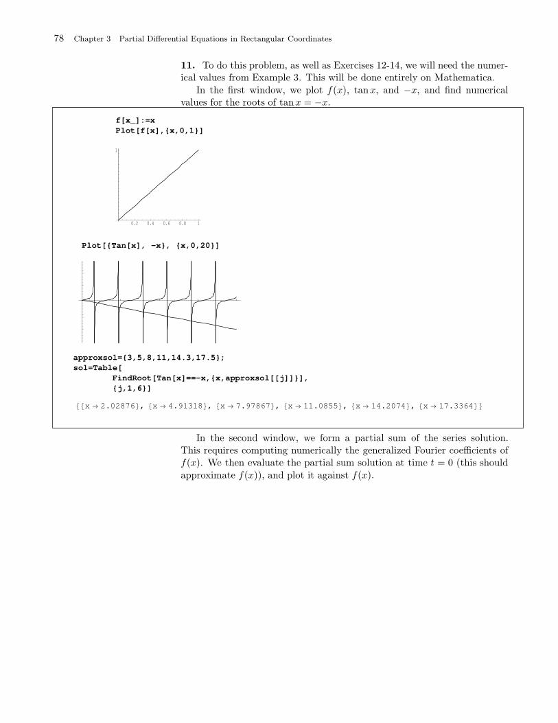
78 Chapter 3 Partial Differential Equations in Rectangular Coordinates
11. To do this problem, as well as Exercises 12-14, we will need the numer-ical values from Example 3. This will be done entirely on Mathematica.
In the first window, we plot f(x), tanx, and −x, and find numericalvalues for the roots of tanx = −x.
f[x_]:=x
Plot[f[x],x,0,1]
0.2 0.4 0.6 0.8 1
1
Plot[Tan[x], -x, x,0,20]
approxsol=3,5,8,11,14.3,17.5;
sol=Table[
FindRoot[Tan[x]==-x,x,approxsol[[j]]],
j,1,6]
x 2.02876 , x 4.91318 , x 7.97867 , x 11.0855 , x 14.2074 , x 17.3364
In the second window, we form a partial sum of the series solution.
This requires computing numerically the generalized Fourier coefficients off(x). We then evaluate the partial sum solution at time t = 0 (this should
approximate f(x)), and plot it against f(x).
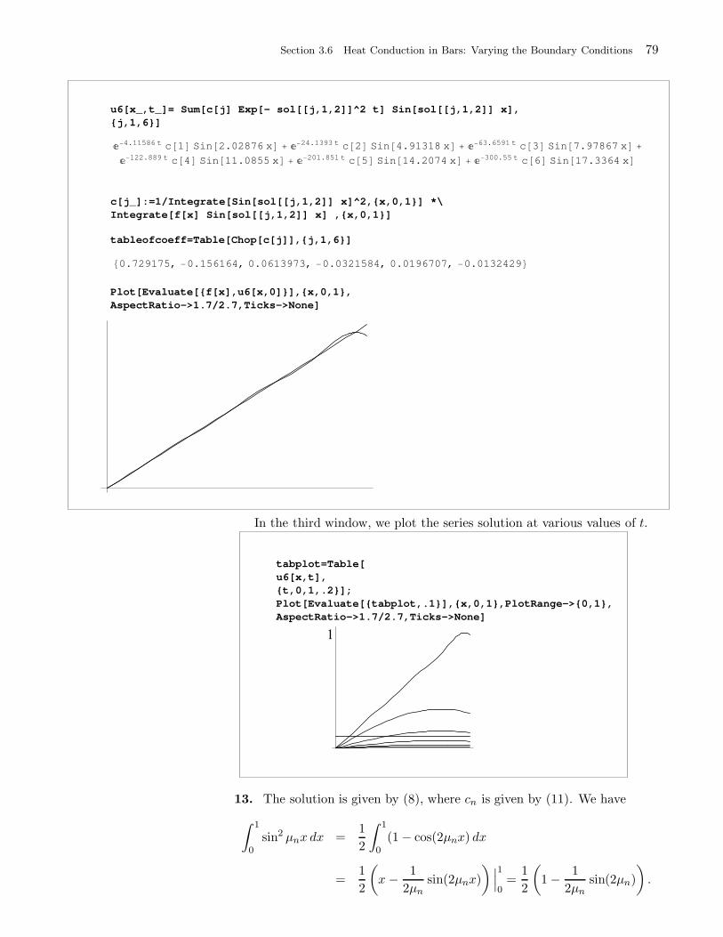
Section 3.6 Heat Conduction in Bars: Varying the Boundary Conditions 79
u6[x_,t_]= Sum[c[j] Exp[- sol[[j,1,2]]^2 t] Sin[sol[[j,1,2]] x],
j,1,6]
4.11586 t c 1 Sin 2.02876 x 24.1393 t c 2 Sin 4.91318 x 63.6591 t c 3 Sin 7.97867 x122.889 t c 4 Sin 11.0855 x 201.851 t c 5 Sin 14.2074 x 300.55 t c 6 Sin 17.3364 x
c[j_]:=1/Integrate[Sin[sol[[j,1,2]] x]^2,x,0,1] *\
Integrate[f[x] Sin[sol[[j,1,2]] x] ,x,0,1]
tableofcoeff=Table[Chop[c[j]],j,1,6]
0.729175, 0.156164, 0.0613973, 0.0321584, 0.0196707, 0.0132429
Plot[Evaluate[f[x],u6[x,0]],x,0,1,
AspectRatio->1.7/2.7,Ticks->None]
In the third window, we plot the series solution at various values of t.
tabplot=Table[
u6[x,t],
t,0,1,.2];
Plot[Evaluate[tabplot,.1],x,0,1,PlotRange->0,1,
AspectRatio->1.7/2.7,Ticks->None]
13. The solution is given by (8), where cn is given by (11). We have
∫ 1
0
sin2 µnx dx =1
2
∫ 1
0
(1 − cos(2µnx) dx
=1
2
(x − 1
2µnsin(2µnx)
) ∣∣∣1
0=
1
2
(1 − 1
2µnsin(2µn)
).
80 Chapter 3 Partial Differential Equations in Rectangular Coordinates
Since µn is a solution of tanµ = −µ, we have sinµn = −µn cosµn, so
sin 2µn = 2 sinµn cosµn = −2µn cos2 µn,
and hence ∫ 1
0sin2 µnx dx =
1
2
(1 + cos2 µn
).
Also, ∫ 1/2
0
sinµnx dx =1
µn
(1− cos
µn
2
).
Applying (11), we find
cn =
∫ 1/2
0100 sinµnx dx
/∫ 1
0sin2 µnx dx
=100
µn
(1 − cos
µn
2
)/
1
2
(1 + cos2 µn
)
=200(1 − cos µn
2
)
µn (1 + cos2 µn).
Thus the solution is
u(x, t) =
∞∑
n=1
200(1− cos µn
2
)
µn (1 + cos2 µn)e−µ2
nt sinµnx.
15. Following the solution in Example 2, we arrive at the following equa-tions
T ′ − kc2T = 0,
X ′′ − kX = 0, X ′(0) = 0, X ′(L) = −κX(L),
where k is a separation constant. If k = 0 then
X ′′ = 0 ⇒ X = ax+ b,
X ′(0) = 0 ⇒ a = 0
X ′(L) = −κX(L) ⇒ b = 0;
so k = 0 leads to trivial solutions. If k = α2 > 0, then, as in the text,we conclude that X = 0. This leaves the case k = −µ2 < 0. In this case
X(x) = c1 cosµx + c2 sinµx. From X ′(0) = 0 it follows that c2 = 0 or X =c2 cosµx. Set c2 = 1 to simplify the presentation. From X ′(L) = −κX(L),we find that −µ sinµL = −κ cosµL. Hence µ is a solution of the equation
µ
κ=
cosµL
sinµLor cotµL =
1
κµ.
Let µn denote the nth positive solution of this equation, and let Xn(x) =cosµnx. Solving the equation for T for each µn, we find
T = Tn = cne−c2µ2
nt
Section 3.6 Heat Conduction in Bars: Varying the Boundary Conditions 81
and hence, by superposing the product solutions, we arrive at
u(x, t) =
∞∑
n=1
cn cosµnxe−c2µ2
nt.
To prove that the Xn’s are orthogonal, see Exercise 19. The proof involves
ideas that will be studied in greater detail in Chapter 6, in the context ofSturm-Liouville theory.
Using the initial condition, it follows that
u(x, 0) = f(x) =
∞∑
n=1
cnXn(x).
Multiplying both sides by Xm and integrating term by term, it follows fromthe orthogonality of the Xn that
∫ L
0f(x)Xm(x) dx =
∞∑
n=1
cn
=0 if m6=n︷ ︸︸ ︷∫ L
0Xn(x)Xm(x) dx .
Hence ∫ L
0f(x)Xm(x) dx = cn
∫ L
0X2
n(x) dx
or
cn =1
κn
∫ L
0f(x)Xn(x) dx
where
κn =
∫ L
0X2
n(x) dx .
Let us evaluate κn. Recall that µn is a solution of cotLµ = 1κµ. We have
κn =
∫ L
0cos2 µnx dx =
1
2
∫ L
0(1 + cos 2µnx) dx
=L
2
1
4µnsin 2µnx
∣∣∣L
0=L
2
1
4µnsin 2µnL.
In order to use what we know about µn, namely, that it is a solution ofcotLµ = 1
κµ, we express the sine in terms of the cotangent, as follows. We
have
sin 2α = 2 sinα cosα =2 sinα cosα
sin2 α+ cos2 α
= 2cotα
cot2 α+ 1,
where the last identity follows upon dividing by cos2 α. Using this in the
expression for κn, we find
κn =L
2+
1
4µn· 2 cotµnL
1 + cot2 µnL
=L
2+
1
2µn
(µn/κ)
1 + (µn/κ)2
=L
2+
κ
2(κ2 + µ2n).
82 Chapter 3 Partial Differential Equations in Rectangular Coordinates
17. Part (a) is straightforward as in Example 2. We omit the details thatlead to the separated equations:
T ′ − kT = 0,
X ′′ − kX = 0, X ′(0) = −X(0), X ′(1) = −X(1),
where k is a separation constant.(b) If k = 0 then
X ′′ = 0 ⇒ X = ax + b,
X ′(0) = −X(0) ⇒ a = −bX ′(1) = −X(1) ⇒ a = −(a+ b) ⇒ 2a = −b;
⇒ a = b = 0.
So k = 0 leads to trivial solutions.(c) If k = α2 > 0, then
X ′′ − µ2X = 0 ⇒ X = c1 coshµx + c2 sinhµx;
X ′(0) = −X(0) ⇒ µc2 = −c1X ′(1) = −X(1) ⇒ µc1 sinhµ+ µc2 coshµ = −c1 coshµ− c2 sinhµ
⇒ µc1 sinhµ− c1 coshµ = −c1 coshµ− c2 sinhµ
⇒ µc1 sinhµ = −c2 sinhµ
⇒ µc1 sinhµ =c1µ
sinhµ.
Since µ 6= 0, sinhµ 6= 0. Take c1 6= 0 and divide by sinhµ and get
µc1 =c1µ
⇒ µ2 = 1 ⇒ k = 1.
So X = c1 coshx+ c2 sinhx. But c1 = −c2, so
X = c1 coshx+ c2 sinhx = c1 coshx − c1 sinhx = c1e−x.
Solving the equation for T , we find T (t) = et; thus we have the productsolution
c0e−xet,
where, for convenience, we have used c0 as an arbitrary constant.(d) If k = −α2 < 0, then
X ′′ + µ2X = 0 ⇒ X = c1 cosµx+ c2 sinµx;
X ′(0) = −X(0) ⇒ µc2 = −c1X ′(1) = −X(1) ⇒ −µc1 sinµ+ µc2 cosµ = −c1 cosµ− c2 sinµ
⇒ −µc1 sinµ− c1 cosµ = −c1 cosµ− c2 sinµ
⇒ −µc1 sinµ = −c2 sinµ
⇒ −µc1 sinµ =c1µ
sinµ.
Since µ 6= 0, take c1 6= 0 (otherwise you will get a trivial solution) and divideby c1 and get
µ2 sinµ = − sinµ ⇒ sinµ = 0 ⇒ µ = nπ,
Section 3.6 Heat Conduction in Bars: Varying the Boundary Conditions 83
where n is an integer. So X = c1 cosnπx+ c2 sinnπx. But c1 = −c2µ, so
X = −c1(nπ cosnπx− sinnπx
).
Call Xn = nπ cosnπx− sinnπx.
(e) To establish the orthogonality of theXn’s, treat the case k = 1 separately.For k = −µ2, we refer to the boundary value problem
X ′′ + µ2nX = 0, X(0) = −X ′(0), X(1) = −X ′(1),
that is satisfied by the Xn’s, where µn = nπ. We establish orthogonalityusing a trick from Sturm-Liouville theory (Chapter 6, Section 6.2). Since
X ′′m = µ2
mXm and X ′′n = µ2
nXn,
multiplying the first equation by Xn and the second by Xm and then sub-
tracting the resulting equations, we obtain
XnX′′m = µ2
mXmXn and XmX′′n = µ2
nXnXm
XnX′′m −XmX
′′n = (µ2
n − µ2m)XmXn(
XnX′m −XmX
′n
)′= (µ2
n − µ2m)XmXn
where the last equation follows by simply checking the validity of the identityXnX
′′m −XmX
′′n =
(XnX
′m −XmX
′n
)′. So
(µ2n − µ2
m)
∫ 1
0Xm(x)Xn(x) dx =
∫ 1
0
(Xn(x)X ′
m(x)−Xm(x)X ′n(x)
)′dx
= Xn(x)X ′m(x)−Xm(x)X ′
n(x)∣∣∣1
0,
because the integral of the derivative of a function is the function itself. Nowwe use the boundary conditions to conclude that
Xn(x)X ′m(x)−Xm(x)X ′
n(x)∣∣∣1
0
= Xn(1)X ′m(1)−Xm(1)X ′
n(1)−Xn(0)X ′m(0) +Xm(0)X ′
n(0)
= −Xn(1)Xm(1) +Xm(1)Xn(1) +Xn(0)Xm(0)−Xm(0)Xn(0)
= 0.
Thus the functions are orthogonal. We still have to verify the orthogonalitywhen one of the Xn’s is equal to e−x. This can be done by modifying theargument that we just gave.
(f) Superposing the product solutions, we find that
u(x, t) = c0e−xet +
∞∑
n=1
cnTn(t)Xn(x).
Using the initial condition, it follows that
u(x, 0) = f(x) = c0e−x +
∞∑
n=1
cnXn(x).
The coefficients in this series expansion are determined by using the orthog-onality of the Xn’s in the usual way. Let us determine c0. Multiplying both
84 Chapter 3 Partial Differential Equations in Rectangular Coordinates
sides by e−x and integrating term by term, it follows from the orthogonalityof the Xn that
∫ 1
0f(x)e−x dx = c0
∫ 1
0e−2xdx+
∞∑
n=1
cn
=0︷ ︸︸ ︷∫ 1
0Xn(x)e−x dx .
Hence ∫ 1
0
f(x)e−x dx = c0
∫ 1
0
e−2xdx = c01 − e−2
2.
Thus
c0 =2e2
e2 − 1
∫ 1
0f(x)e−x dx.
In a similar way, we prove that
cn =1
κn
∫ 1
0f(x)Xn(x) dx
where
κn =
∫ 1
0X2
n(x) dx .
This integral can be evaluated as we did in Exercise 15 or by straightforward
computations, using the explicit formula for the Xn’s, as follows:
∫ 1
0X2
n(x) dx =
∫ 1
0
(nπ cosnπx− sinnπx
)2dx
=
∫ 1
0
(n2π2 cos2 nπx+ sin2 nπx− 2nπ cos(nπx) sin(nπx)
)dx
=
=(n2π2)/2︷ ︸︸ ︷∫ 1
0n2π2 cos2 nπx dx+
=1/2︷ ︸︸ ︷∫ 1
0sin2 nπx dx
−2nπ
=0︷ ︸︸ ︷∫ 1
0cos(nπx) sin(nπx) dx
=n2π2 + 1
2.
19. (a) Following the solution in Exercise 16, we arrive at the following
equations
T ′ − kT = 0,
X ′′ − kX = 0, X ′(0) = X(0), X ′(1) = −X(1),
where k is a separation constant. We will not repeat the details.(b) If k = 0 then
X ′′ = 0 ⇒ X = ax+ b,
X ′(1) = −X(1) ⇒ a = −a ⇒ a = 0
X ′(0) = X(0) ⇒ a = b = 0;
Section 3.6 Heat Conduction in Bars: Varying the Boundary Conditions 85
so k = 0 leads to trivial solutions. If k = α2 > 0, then
X ′′ − α2X = 0 ⇒ X = c1 coshαx+ c2 sinhαx,
X(0) = c1, X′(0) = αc2,
X(1) = c1 coshα + c2 sinhα, X ′(1) = αc1 sinhα+ αc2 coshα,
X ′(0) = X(0) ⇒ c1 = αc2
X ′(1) = −X(1) ⇒ −(c1 coshα+ c2 sinhα) = αc1 sinhα+ αc2 coshα.
Using αc2 = c1, we obtain from the last equation
−(c1 coshα+c1α
sinhα) = αc1 sinhα+ c1 coshα.
Either c1 = 0, in which case we have a trivial solution, or
−(α coshα+ sinhα) = α(α sinhα+ coshα)
−2α coshα = (α2 + 1) sinhα.
If α > 0, then the left side is < 0 while the right side is > 0. So there areno positive solutions. Also, if α < 0, then the left side is > 0 while the right
side is < 0. So there are no negative solutions. Hence the only solution thatsatisfies the equation and the boundary conditions is the trivial solution in
the case k = α2 > 0.(c) The separation constant must be negative: k = −µ2 < 0. In this case
X(x) = c1 cosµx + c2 sinµx. From X ′(0) = X(0) it follows that c1 = µc2.Hence X(x) = c2µ cosµx + c2 sinµx, where c2 6= 0. From X ′(1) = −X(1),
we find that −c2µ2 sinµ + c2µ cosµ = −c2µ cosµ − c2 sinµ. Hence µ is asolution of the equation
−µ2 sinµ+ µ cosµ = −µ cosµ− sinµ ⇒ 2µ cosµ = (µ2 − 1) sinµ
Note that µ = ±1 s not a solution and cosµ = 0 is not a possibility, since
this would imply sinµ = 0 and the two equations have no common solutions.So we can divide by cosµ(µ2 −1) and conclude that µ satisfies the equation
tanµ = 2µµ2−1
. This equation has infinitely many solutions µ = ±µn, thatcan be seen on a graph. We take only the positive µn since we do not gain
any new solutions in X for −µn. Write the corresponding solutions
X = Xn = cn(µn cosµnx+ sinµn), (n = 1, 2, , . . .)
The corresponding solutions in T are
Tn(t) = e−µ2nt.
(e) We can prove that the Xn are orthogonal on the interval [0, 1] as follows.
(The ideas in the proof will be studied in greater detail in Chapter 6, in thecontext of Sturm-Liouville theory. They will also appear when we establishthe orthogonality of Bessel functions (Chapter 4) and Legendre polynomials
(Chapter 5).) We will not need the explicit formulas for Xn and Xm. Wewill work with the fact hat these are both solutions of the same boundary
value problem
X ′′ + µ2X = 0, X(0) = X ′(0), X(1) = −X ′(1),
86 Chapter 3 Partial Differential Equations in Rectangular Coordinates
corresponding to different values of µ = µm and µ = µn, with µm 6= µn. So
X ′′m = µ2
mXm and X ′′n = µ2
nXn.
Multiplying the first equation by Xn and the second by Xm and then sub-tracting the resulting equations, we obtain
XnX′′m = µ2
mXmXn and XmX′′n = µ2
nXnXm
XnX′′m −XmX
′′n = (µ2
n − µ2m)XmXn(
XnX′m −XmX
′n
)′= (µ2
n − µ2m)XmXn
where the last equation follows by simply checking the validity of the identityXnX
′′m −XmX
′′n =
(XnX
′m −XmX
′n
)′. So
(µ2n − µ2
m)
∫ 1
0Xm(x)Xn(x) dx =
∫ 1
0
(Xn(x)X ′
m(x)−Xm(x)X ′n(x)
)′dx
= Xn(x)X ′m(x)−Xm(x)X ′
n(x)∣∣∣1
0,
because the integral of the derivative of a function is the function itself. Nowwe use the boundary conditions to conclude that
Xn(x)X ′m(x)−Xm(x)X ′
n(x)∣∣∣1
0
= Xn(1)X ′m(1)−Xm(1)X ′
n(1)−Xn(0)X ′m(0) +Xm(0)X ′
n(0)
= −Xn(1)Xm(1) +Xm(1)Xn(1)−Xn(0)Xm(0) +Xm(0)Xn(0)
= 0.
Thus the functions are orthogonal.
(f) Superposing the product solutions, we find that
u(x, t) =
∞∑
n=1
cnTn(t)Xn(x).
Using the initial condition, it follows that
u(x, 0) = f(x) =
∞∑
n=1
cnXn(x).
Multiplying both sides by Xm and integrating term by term, it follows from
the orthogonality of the Xn that
∫ 1
0
f(x)Xm(x) dx =∞∑
n=1
cn
=0 if m6=n︷ ︸︸ ︷∫ 1
0
Xn(x)Xm(x) dx .
Hence ∫ 1
0f(x)Xm(x) dx = cn
∫ 1
0X2
n(x) dx
or
cn =1
κn
∫ 1
0
f(x)Xn(x) dx
where
κn =
∫ 1
0X2
n(x) dx .
Section 3.7 The Two Dimensional Wave and Heat Equations 87
Solutions to Exercises 3.7
3. We use the double sine series solution that is outlined in the text.
u(x, y, t) =
∞∑
n=1
∞∑
m=1
(Bmn cos λmnt+B∗mn sinλmnt) sin
mπx
asin
nπy
b,
where a and b are the dimensions of the membrane,
λmn = cπ
√m2
a2+n2
b2,
Bmn =4
ab
∫ b
0
∫ a
0f(x, y) sin
mπx
asin
nπy
bdx dy,
B∗mn =
4
abλmn
∫ b
0
∫ a
0
g(x, y) sinmπx
asin
nπy
bdx dy.
Applying these formulas in our case, we find
λmn =√m2 + n2,
B∗mn =
2
λ1,2= 2√
5if (m, , n) = (1, 2),
0 otherwise,
because of the orthogonality of the functions sinmπx sinnπy and the factthat g contains only the function sinπx sin 2ıy. We also have
Bmn = 4
∫ 1
0
∫ 1
0
x(1− x)y(1 − y) sinmπx sinnπy dx dy
= 4
∫ 1
0
x(1− x) sinmπx dx
∫ 1
0
y(1 − y) sinnπy dy
=
64
(mnπ2)3if m and n are both odd,
0 otherwise.
Refer to Example 1 of this section or Exercise 9, Section 3.3, for the com-
putation of the definite integrals. Thus
u(x, y, t) =∞∑
k=0
∞∑
l=0
64 sin((2k+ 1)πx) sin((2l+ 1)πy)
((2k + 1)(2l+ 1)π2)3cos√
(2k + 1)2 + (2l+ 1)2t
+2√5
sinπx sin(2πy) sin(√
5 t).
5. We proceed as in Exercise 3. We have
u(x, y, t) =
∞∑
n=1
∞∑
m=1
(Bmn cos λmnt+B∗mn sinλmnt) sinmπx sinnπy,
where λmn =√m2 + n2, Bmn = 0, and
B∗mn =
4√m2 + n2
∫ 1
0
∫ 1
0sinmπx sinnπy dx dy
=4√
m2 + n2
∫ 1
0sinmπx dx
∫ 1
0sinnπy dy
=
16√
m2+n2(mn)π2if m and n are both odd,
0 otherwise.
88 Chapter 3 Partial Differential Equations in Rectangular Coordinates
Thus
u(x, y, t) =∞∑
k=0
∞∑
l=0
16 sin((2k+ 1)πx) sin((2l+ 1)πy)√(2k + 1)2 + (2l+ 1)2 (2k+ 1)(2l+ 1)π2
sin√
(2k+ 1)2 + (2l+ 1)2t
Section 3.8 Laplace’s Equation in Rectangular Coordinates 89
Solutions to Exercises 3.8
1. The solution is given by
u(x, y) =
∞∑
n=1
Bn sin(nπx) sinh(nπy),
where
Bn =2
sinh(2nπ)
∫ 1
0x sin(nπx) dx
=2
sinh(2nπ)
[−x cos(nπ x)
nπ+
sin(nπ x)
n2 π2
] ∣∣∣1
0
=2
sinh(2nπ)
−(−1)n
nπ=
2
sinh(2nπ)
(−1)n+1
nπ.
Thus,
u(x, y) =2
π
∞∑
n=1
(−1)n+1
n sinh(2nπ)sin(nπx) sinh(nπy).
3. The solution is given by
u(x, y) =
∞∑
n=1
An sin(nπx
2) sinh(
nπ
2(1− y)) +
∞∑
n=1
Dn sin(nπy) sinh(nπx),
where
An =2
sinh(nπ2 )
∫ 2
0100 sin(
nπx
2) dx
=2
sinh(nπ2 )
[−200
nπcos
nπx
2
] ∣∣∣2
0
=200
nπ(1 − cos(−1)n)
=
400nπ if n is odd,
0 if n is even;
and
Dn =2
sinh(2nπ)
∫ 1
0100(1− y) sin(nπy) dy
=200
sinh(2nπ)
[(−1 + y) cos(nπ y)
nπ− sin(nπ y)
n2 π2
] ∣∣∣1
0
=200
nπ sinh(2nπ)
Thus,
u(x, y) =400
π
∞∑
k=0
sin((2k+1)πx
2 ) sinh((2k+1)π
2 (1− y))
(2k+ 1) sinh( (2k+1)π2 )
+200
π
∞∑
n=1
sin(nπy) sinh(nπx)
nπ sinh(2nπ).
5. Start by decomposing the problem into four subproblems as describedby Figure 3. Let uj(x, y) denote the solution to problem j (j = 1, 2, 3, 4).
90 Chapter 3 Partial Differential Equations in Rectangular Coordinates
Each uj consists of only one term of the series solutions, because of theorthogonality of the sine functions. For example, to compute u1, we have
u1(x, y) =
∞∑
n=1
An sinnπx sinh[nπ(1− y)],
where
An =2
sinhnπ
∫ 1
0sin 7πx sinnπx dx.
Since the integral is 0 unless n = 7 and, when n = 7,
A7 =2
sinh 7π
∫ 1
0
sin2 7πx dx =1
sinh7π.
Thus
u1(x, y) =1
sinh7πsin 7πx sinh[7π(1− y)].
In a similar way, appealing to the formulas in the text, we find
u2(x, y) =1
sinhπsinπx sinh(πy)
u3(x, y) =1
sinh 3πsinh[3π(1− x)] sin(3πy)
u4(x, y) =1
sinh 6πsinh6πx sin(6πy);
u(x, y) = u1(x, y) + u2(x, y) + u3(x, y) + u4(x, y)
=1
sinh 7πsin 7πx sinh[7π(1− y)] +
1
sinhπsin(πx) sinh(πy)
+1
sinh 3πsinh[3π(1− x)] sin(3πy) +
1
sinh6πsinh(6πx) sin(6πy)
7. (a) From Example 1, the solution is
u(x, y) =
∞∑
n=1
Bn sinnπx
asinh
nπy
a,
where
Bn =2
a sinh(nπba )
∫ a
0f2(x) sin
nπx
adx
=1
sinh(nπba )
bn︷ ︸︸ ︷2
a
∫ a
0f2(x) sin
nπx
adx
=1
sinh(nπba )
bn,
where bn is the sine Fourier coefficient of f2(x), as given by (3), Section 2.4.Replacing Bn by its value in terms of bn in the series solution, we obtain
Section 3.8 Laplace’s Equation in Rectangular Coordinates 91
(a). In the general case, we refer the series solution (9). It is easy to see, aswe just did, that
An =1
sinh(nπba )
bn(f1)︷ ︸︸ ︷2
a
∫ a
0f1(x) sin
nπx
adx =
1
sinh(nπba )
bn(f1),
Cn =1
sinh(nπab )
bn(g1)︷ ︸︸ ︷2
b
∫ b
0g1(y) sin
nπy
bdy =
1
sinh(nπab )
bn(g1),
Dn =1
sinh(nπab )
bn(g2)︷ ︸︸ ︷2
b
∫ b
0
g2(y) sinnπy
bdy =
1
sinh(nπab )
bn(g2),
where, bn(f) denotes the nth sine Fourier coefficient of f . So, in terms of
the Fourier coefficients of the boundary functions, the general solution (9)becomes
u(x, y) =
∞∑
n=1
bn(f1) sinnπ
ax
sinh nπa (b− y)
sinh nπba
+
∞∑
n=1
bn(f2) sinnπ
ax
sinh nπa y
sinh nπba
∞∑
n=1
bn(g1) sinnπ
bysinh nπ
b (a− x)
sinh nπab
+∞∑
n=1
bn(g2) sinnπ
bysinh nπ
b x
sinh nπab
.
92 Chapter 3 Partial Differential Equations in Rectangular Coordinates
Solutions to Exercises 3.9
1. We apply (2), with a = b = 1:
u(x, y) =
∞∑
n=1
∞∑
m=1
Emn sinmπx sinnπy,
where
Emn =−4
π2(m2 + n2)
∫ 1
0
∫ 1
0x sinmπx sinnπy dx dy
=−4
π2(m2 + n2)
∫ 1
0
x sinmπx dx
=1−(−1)n
nπ︷ ︸︸ ︷∫ 1
0
sinnπy dy
=−4
π4(m2 + n2)
1 − (−1)n
n
(−x cos(mπx)
m+
sin(mx)
m2π
) ∣∣∣1
0
=4
π4(m2 + n2)
1 − (−1)n
n
(−1)m
m.
Thus
u(x, y) =8
π4
∞∑
k=0
∞∑
m=1
(−1)m
(m2 + (2k + 1)2)m(2k+ 1)sinmπx sin((2k+ 1)πy).
3. We use the solution in the text:
u(x, y) = u1(x, y) + u2(x, y) =
∞∑
n=1
∞∑
m=1
Emn sinmπx sinnπy + u2(x, y),
where u1 is the solution of an associated Poisson problem with zero boundarydata, and u2 is the solution of the Dirichlet problem with the given boundary
data. We have
Emn =−4
π2(m2 + n2)
∫ 1
0
∫ 1
0sinπx sinmπx sinnπy dx dy
=−4
π2(m2 + n2)
0 if m6=1, 1/2 if m=1︷ ︸︸ ︷∫ 1
0
sinπx sinmπx dx
=1−(−1)n
nπ︷ ︸︸ ︷∫ 1
0
sinnπy dy
=
0 if m 6= 1,
−2π3(1+n2)
(1−(−1)n)n if m = 1
.
Thus
u1(x, y) =−4
π3sin(πx)
∞∑
k=0
1
(1 + (2k + 1)2)(2k + 1)sin((2k+ 1)πy).
To find u2, we apply the results of Section 3.8. We have
∞∑
n=1
Bn sinnπx sinhnπy,
Section 3.9 Poisson’s Equation: The Method of Eigenfunction Expansions 93
where
Bn =2
sinh(nπ)
∫ 1
0x sinnπx dx
=2
sinh(nπ)
(−1)n+1
nπ.
Thus2
π
∞∑
n=1
(−1)n+1
n sinh(nπ)sinnπx sinhnπy,
and so
u(x, y) =−4
π3sin(πx)
∞∑
k=0
1
(1 + (2k + 1)2)(2k+ 1)sin((2k+ 1)πy)
+2
π
∞∑
n=1
(−1)n+1
n sinh(nπ)sinnπx sinhnπy.
5. We will use an eigenfunction expansion based on the eigenfunctions
φ(x, y) = sinmπx sinnπy, where ∆π(x, y) = −π2(m2+n2
)sinmπx sinnπy.
So plug
u(x, y) =
∞∑
n=1
∞∑
m=1
Emn sinmπx sinnπy
into the equation ∆u = 3u− 1, proceed formally, and get
∆ (∑∞
n=1
∑∞m=1 Emn sinmπx sinnπy) = 3
∑∞n=1
∑∞m=1 Emn sinmπx sinnπy − 1
∑∞n=1
∑∞m=1 Emn∆ (sinmπx sinnπy) = 3
∑∞n=1
∑∞m=1 Emn sinmπx sinnπy − 1
∑∞n=1
∑∞m=1 −Emnπ
2(m2 + n2
)sinmπx sinnπy
= 3∑∞
n=1
∑∞m=1 Emn sinmπx sinnπy − 1
∑∞n=1
∑∞m=1
(3 + π2
(m2 + n2
))Emn sinmπx sinnπy = 1.
Thinking of this as the double sine series expansion of the function identically
1, it follows that(3+π2
(m2 +n2
))Emn are double Fourier sine coefficients,
given by (see (8), Section 3.7)
(3 + π2
(m2 + n2
))Emn = 4
∫ 1
0
∫ 1
0
sinmπx sinnπy dx dy
= 41 − (−1)m
mπ
1 − (−1)n
nπ
=
0 if either m or n is even,
16π2m n
if both m and n are even..
Thus
Emn =
0 if either m or n is even,
16
π2m n(3+π2
(m2+n2
)) if both m and n are even,
and so
u(x, y) =16
π2
∞∑
k=0
∞∑
l=0
sin((2k+ 1)πx) sin((2l+ 1)πy)
(2k + 1) (2l+ 1)(3 + π2
((2k + 1)2 + (2l+ 1)2
)) .
94 Chapter 3 Partial Differential Equations in Rectangular Coordinates
Solutions to Exercises 3.10
1. We use a combination of solutions from (2) and (3) and try a solution
of the form
u(x, y) =
∞∑
n=1
sinmx[Am coshm(1 − y) +Bm sinhmy
].
(If you have tried a different form of the solution, you can still do the prob-lem, but your answer may look different from the one derived here. The
reason for our choice is to simplify the computations that follow.) Theboundary conditions on the vertical sides are clearly satisfied. We now
determine Am and Bm so as to satisfy the conditions on the other sides.Starting with u(1, 0) = 100, we find that
100 =
∞∑
m=1
Am coshm sinmx.
Thus Am coshm is the sine Fourier coefficient of the function f(x) = 100.Hence
Am coshm =2
π
∫ π
0
100 sinmxdx ⇒ Am =200
πm coshm[1 − (−1)m] .
Using the boundary condition uy(x, 1) = 0, we find
0 =∞∑
m=1
sinmx[Am(−m) sinh[m(1− y)] +mBm coshmy
]∣∣∣y=1
.
Thus
0 =
∞∑
m=1
mBm sinmx coshm.
By the uniqueness of Fourier series, we conclude that mBm coshm = 0 for
all m. Since m coshm 6= 0, we conclude that Bm = 0 and hence
u(x, y) =200
π
∞∑
m=1
[1 − (−1)m]
m coshmsinmx cosh[m(1− y)]
=400
π
∞∑
k=0
sin[(2k+ 1)x]
(2k+ 1) cosh(2k + 1)cosh[(2k+ 1)(1− y)].
3. Try a solution of the form
u(x, y) =∞∑
n=1
sinmx[Am coshm(1 − y) +Bm sinhmy
].
Using the boundary conditions on the horizontal sides, starting with uy(x, 1) =
0, we find
0 =∞∑
n=1
mBm sinmx coshm.
Thus Bm = 0 for all m and so
u(x, y) =
∞∑
n=1
sinmxAm coshm(1− y).
Section 3.10 Neumann and Robin Conditions 95
We now work with the Robin condition u(x, 0) + 2uy(x, 0) = g(x) and get
∞∑
n=1
sinmxAm coshm− 2
∞∑
n=1
sinmxAmm sinhm = g(x)
⇒ g(x) =
∞∑
n=1
Am sinmx[coshm− 2m sinhm
]
⇒ Am
[coshm− 2m sinhm
]=
2
π
∫ π
0g(x) sinmxdx
⇒ Am =2
π[coshm− 2m sinhm]
∫ π
0g(x) sinmxdx,
which determines the solution.
5. We combine solutions of different types from Exercise 4 and try a solution
of the form
u(x, y) = A0 +B0y +
∞∑
m=1
cosmπ
ax[Am cosh[
mπ
a(b− y)] +Bm sinh[
mπ
ay]].
Using the boundary conditions on the horizontal sides, starting with uy(x, b) =
0, we find that
0 = B0 +
∞∑
m=1
mπ
aBm cos
mπ
ax cosh
[mπab].
Thus B0 = 0 and Bm = 0 for all m ≥ 1 and so
A0 +
∞∑
m=1
Am cosmπ
ax cosh[
mπ
a(b− y)].
Now, using u(x, 0) = g(x), we find
g(x) = A0 +
∞∑
m=1
Am cosh[mπ
ab] cos
mπ
ax.
Recognizing this as a cosine series, we conclude that
A0 =1
a
∫ a
0g(x) dx
and
Am cosh[mπ
ab] =
2
a
∫ a
0g(x) cos
mπ
ax dx;
equivalently, for m ≥ 1,
Am =2
a cosh[mπa b]
∫ a
0
g(x) cosmπ
ax dx.
7. The solution is immediate form (5) and (6). We have
u(x, y) =
∞∑
m=1
Bm sinmx sinhmy,
96 Chapter 3 Partial Differential Equations in Rectangular Coordinates
where Bm are given by (6) with f(x) = sin 2x. By the orthogonality of thetrigonometric system, we have Bm = 0 for all m 6= 2 and B2 = 1
2 cosh(2π) .Thus
u(x, y) =1
2 cosh(2π)sin 2x sinh2y.
9. We follow the solution in Example 3. We have
u(x, y) = u1(x, y) + u2(x, y),
where
u1(x, y) =
∞∑
m=1
Bm sinmx sinhmy,
with
Bm =2
πm cosh(mπ)
∫ π
0sinmxdx =
2
πm2 cosh(mπ)(1 − (−1)m);
and
u2(x, y) =
∞∑
m=1
Am sinmx cosh[m(π − y)],
with
Am =2
π cosh(mπ)
∫ π
0sinmxdx =
2
πm cosh(mπ)(1 − (−1)m).
Hence
u(x, y) =2
π
∞∑
m=1
(1− (−1)m)
m cosh(mπ)sinmx
[sinhmy
m+ cosh[m(π − y)]
]
=4
π
∞∑
k=0
sin(2k+ 1)x
(2k+ 1) cosh[(2k+ 1)π]
[sinh[(2k+ 1)y]
(2k+ 1)+ cosh[(2k+ 1)(π− y)]
].
Section 4.1 The Laplacian in Various Coordinate Systems 97
Solutions to Exercises 4.1
1. We could use Cartesian coordinates and compute ux, uy, uxx, and uyy
directly from the definition of u. Instead, we will use polar coordinates,because the expression x2 +y2 = r2, simplifies the denominator, and thus it
is easier to take derivatives. In polar coordinates,
u(x, y) =x
x2 + y2=r cos θ
r2=
cos θ
r= r−1 cos θ .
So
ur = −r−2 cos θ, urr = 2r−3 cos θ, uθ = −r−1 sin θ, uθθ = −r−1 cos θ.
Plugging into (1), we find
∇2u = urr +1
rur +
1
r2uθθ =
2 cos θ
r3− cos θ
r3− cos θ
r3= 0 (if r 6= 0).
If you used Cartesian coordinates, you should get
uxx =2x(x2 − 3y2)
(x2 + y2)2and uyy = −2x(x2 − 3y2)
(x2 + y2)2.
3. In polar coordinates:
u(r, θ) =1
r⇒ ur = − 1
r2, urr =
2
r3, uθ = 0, uθθ = 0.
Plugging into (1), we find
∇2u = urr +1
rur +
1
r2uθθ =
2
r3− 1
r3=
1
r3(for r 6= 0).
Thus u does not satisfy Laplace’s equation.
5. In spherical coordinates:
u(r, θ, φ) = r3 ⇒ urr = 6r, uθ = 0, uθθ = 0, uφφ = 0.
Plugging into (3), we find
∇2u =∂2u
∂r2+
2
r
∂u
∂r+
1
r2
(∂2u
∂θ2+ cot θ
∂u
∂θ+ csc2 θ
∂2u
∂φ2
)= 6r + 6r = 12r.
7. In spherical coordinates:
u(r, θ, φ) = r−1 ⇒ ur = − 1
r2, urr =
2
r3, uθ = 0, uθθ = 0, uφφ = 0.
Plugging into (3), we find
∇2u =∂2u
∂r2+
2
r
∂u
∂r+
1
r2
(∂2u
∂θ2+cot θ
∂u
∂θ+csc2 θ
∂2u
∂φ2
)=
2
r3− 2
r3= 0 (for r 6= 0).
9. (a) If u(r, θ, φ) depends only on r, then all partial derivatives of u withrespect to θ and φ are 0. So (3) becomes
∇2u =∂2u
∂r2+
2
r
∂u
∂r+
1
r2
(∂2u
∂θ2+ cot θ
∂u
∂θ+ csc2 θ
∂2u
∂φ2
)=∂2u
∂r2+
2
r
∂u
∂r.
98 Chapter 4 Partial Differential Equations in Polar and Cylindrical Coordinates
(b) If u(r, θ, φ) depends only on r and θ, then all partial derivatives of uwith respect to φ are 0. So (3) becomes
∇2u =∂2u
∂r2+
2
r
∂u
∂r+
1
r2
(∂2u
∂θ2+ cot θ
∂u
∂θ
).
11. (a) This part follows from the fact that differentiation is a linearoperation. Hence
∇2(αu+ βv) = α∇2(u) + β∇2(v).
So if ∇2u = 0 and ∇2v = 0, then ∇2(αu+ βv) = 0, implying that αu + βv
is harmonic.(b) Take u(x, y) = x and v(x, y) = x. Clearly, uxx = uyy = 0 so u and
hence v are harmonic. But uv = x2; so (uv)xx = 2 and (uv)yy = 0. Hence∇2(uv) = 2, implying that uv is not harmonic.(c) If u is harmonic then uxx + uyy = 0. We have
(u2)xx = (2uux)x = 2(ux)2+2uuxx and (u2)yy = (2uuy)y = 2(uy)
2+2uuyy.
If u2 is also harmonic, then
0 = (u2)xx + (u2)yy = 2(ux)2 + 2uuxx + 2(uy)2 + 2uuyy
= 2((ux)2 + (uy)2) + 2u
=0︷ ︸︸ ︷(uxx + uyy)
= 2((ux)2 + (uy)2),
which implies that both ux and uy are identically 0. This latter condi-
tion implies that u is constant on its domain of definition, if the domainis connected. This result is not true if the domain of the function u is not
connected. For example, suppose that u(x, y) = 1 if x > 1 and u(x, y) = −1if x < −1. Clearly, u is not constant and both u and u2 are harmonic. (Forthe definition of connected set, see my book “Applied Complex Analysis and
Partial Differential Equations.”) Examples of connected sets are any disk,the plane, the upper half-plane, any triangular region any annulus.
(d) This part is similar to (c). We suppose that the domain of definition ofthe functions is connected. (Here again, the result is not true if the domain
is not connected.) Suppose that u, v, and u2 + v2 are harmonic. Then
uxx + uyy = 0; vxx + vyy = 0;
2((ux)2 + (uy)
2) + 2u
=0︷ ︸︸ ︷(uxx + uyy)+2((vx)2 + (vy)
2) + 2v
=0︷ ︸︸ ︷(vxx + vyy) .
The last equation implies that (ux)2 + (uy)2 + (vx)2 + (vy)
2 = 0, which, in
turn, implies that ux = uy = vx = vy = 0. Hence u and v are constant.
Section 4.2 Vibrations of a Circular Membrane: Symmetric Case 99
Solutions to Exercises 4.2
1. We appeal to the solution (5) with the coefficients (6). Since f(r) = 0, thenAn = 0 for all n. We have
Bn =1
αnJ1(αn)2
∫ 2
0
J0(αnr
2)r dr
=4
α3nJ1(αn)2
∫ αn
0
J0(s)s ds (let s =αn
2r)
=4
α3nJ1(αn)2
[sJ1(s)]
∣∣∣∣αn
0
=4
α2nJ1(αn)
for all n ≥ 1.
Thus
u(r, t) = 4∞∑
n=1
J0(αnr2 )
α2nJ1(αn)
sin(αnt
2).
3. As in Exercise 1, f(r) = 0 ⇒ An = 0 for all n. We have
Bn =2
αnJ1(αn)2
∫ 12
0
J0(αnr)r dr
=2
α3nJ1(αn)2
∫ αn/2
0
J0(s)s ds
=2
α3nJ1(αn)2
[sJ1(s)]
∣∣∣∣αn/2
0
=J1(
αn
2 )
α2nJ1(αn)2
for all n ≥ 1.
Thus
u(r, t) =
∞∑
n=1
J1(αn
2 )
α2nJ1(αn)2
J0(αnr) sin(αnt).
5. Since g(r) = 0, we have Bn = 0 for all n. We have
An =2
J1(αn)2
∫ 1
0
J0(α1r)J0(αnr)r dr = 0 for n 6= 1 by orthogonality.
For n = 1,
A1 =2
J1(α1)2
∫ 1
0
J0(α1r)2r dr = 1,
where we have used the orthogonality relation (12), Section 4.8, with p = 0. Thus
u(r, t) = J0(α1r) cos(α1t).
7. Using orthogonality as in Exercise 5, since f(r) = J0(α3 r), we find that An = 0for all n 6= 3 and A3 = 1. For the Bn’s, we have
Bn =2
αnJ1(αn)2
∫ 1
0
(1 − r2)J0(αnr)r dr
=2
α5nJ1(αn)2
∫ αn
0
(α2n − s2)J0(s)s ds (let s = αnr).
100 Chapter 4 Partial Differential Equations in Polar and Cylindrical Coordinates
The last integral can be evaluated by parts: u = α2n − s2, du = −2s, J0(s)s ds =
dv, v = sJ1(s). So
Bn =2
α5nJ1(αn)2
[(α2
n − s2)sJ1(s)∣∣αn
0+ 2
∫ αn
0
s2J1(s) ds
]
=4
α5nJ1(αn)2
∫ αn
0
s2J1(s) ds
=4
α5nJ1(αn)2
s2J2(s)
∣∣∣∣αn
0
(by (7), Section 4.8)
=4J2(αn)
α3nJ1(αn)2
=8
α4nJ1(αn)
(using J2(αn) =2
αnJ1(αn)).
Thus
u(r, t) = J0(α3r) cos(α3t) + 8
∞∑
n=1
J0(αnr)
α4nJ1(αn)
sin(αnt).
9. (a) Modifying the solution of Exercise 3, we obtain
u(r, t) =∞∑
n=1
J1(αn/2)
α2ncJ1(αn)2
J0(αnr) sin(αnct).
(b) Under suitable conditions that allow us to interchange the limit and the sum-mation sign (for example, if the series is absolutely convergent), we have, for a given(r, t),
limc→∞
u(r, t) = limc→∞
∞∑
n=1
J1(αn/2)
α2ncJ1(αn)2
J0(αnr) sin(αnct)
=
∞∑
n=1
limc→∞
J1(αn/2)
α2ncJ1(αn)2
J0(αnr) sin(αnct)
= 0,
because limc→∞J1(αn/2)
α2ncJ1(αn)2 = 0 and sin(αnct) is bounded. If we let u1(r, t) denote
the solution corresponding to c = 1 and uc(r, t) denote the solution for arbitraryc > 0. Then, it is easy t check that
uc(r, t) =1
cu1(r, ct).
This shows that if c increases, the time scale speeds proportionally to c, while thedisplacement decreases by a factor of 1
c .
11. (a) With f(r) = 100, we have from Exercise 10,
An =200
a2J1(αn)
∫ a
0
J0(αnr
ar)r dr
=200
α2nJ1(αn)2
∫ αn
0
J0(s)s ds (letαnr
a= s
=200
α2nJ1(αn)2
J1(s)s
∣∣∣∣αn
0
=200
αnJ1(αn).
Hence
u(r, t) = 200
∞∑
n=1
J0(αnr
a )
αnJ1(αn)e−
c2α2nt
a2 .
Section 4.2 Vibrations of a Circular Membrane: Symmetric Case 101
The solution represents the time evolution of the temperature of the disk, startingwith an initial uniform temperature distribution of 100 and with its boundary heldat 0. The top and bottom faces of the disk are assumed to be completely insulatedso that no heat flows through them.(b) The maximum value of the temperature should occur at the center, since heatis being lost only along the circumference of the disk. Of all the points in the disk,the center is least affected by this loss of heat. If we take a = 1, c = 1, and t = 3in the solution to part (a), we obtain
u(r, 3) = 200
∞∑
n=1
J0(αnr)
αnJ1(αn)e−3α2
n .
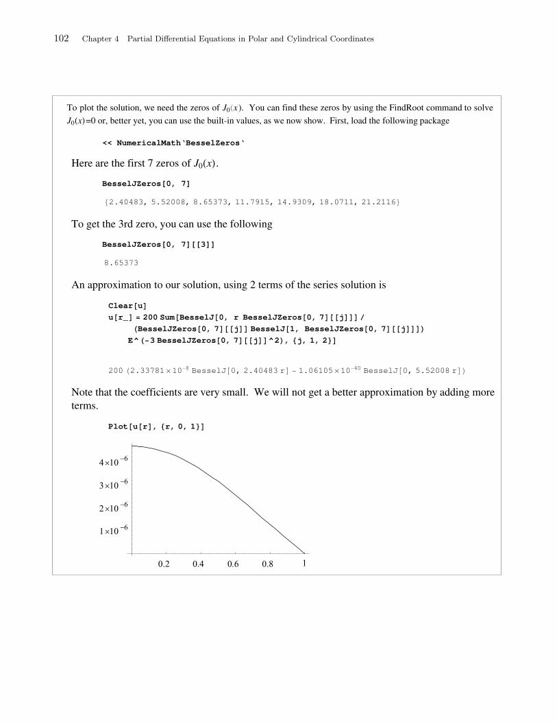
102 Chapter 4 Partial Differential Equations in Polar and Cylindrical Coordinates
To plot the solution, we need the zeros of J0 x). You can find these zeros by using the FindRoot command to solve
J0 x =0 or, better yet, you can use the built-in values, as we now show. First, load the following package
<< NumericalMath‘BesselZeros‘
Here are the first 7 zeros of J0 x .
BesselJZeros[0, 7]
2.40483, 5.52008, 8.65373, 11.7915, 14.9309, 18.0711, 21.2116
To get the 3rd zero, you can use the following
BesselJZeros[0, 7][[3]]
8.65373
An approximation to our solution, using 2 terms of the series solution is
Clear u
u r_ 200 Sum BesselJ 0, r BesselJZeros 0, 7 j
BesselJZeros 0, 7 j BesselJ 1, BesselJZeros 0, 7 j
E^ 3 BesselJZeros 0, 7 j ^2 , j, 1, 2
200 2.33781 10 8 BesselJ 0, 2.40483 r 1.06105 10 40 BesselJ 0, 5.52008 r
Note that the coefficients are very small. We will not get a better approximation by adding more
terms.
Plot u r , r, 0, 1
Section 4.3 Vibrations of a Circular Membrane: General Case 103
Solutions to Exercises 4.3
1. The condition g(r, θ) = 0 implies that a∗mn = 0 = b∗mn. Since f(r, θ) isproportional to sin 2θ, only b2,n will be nonzero, among all the amn and bmn. Thisis similar to the situation in Example 2. For n = 1, 2, . . ., we have
b2,n =2
πJ3(α2,n)2
∫ 1
0
∫ 2π
0
(1 − r2)r2 sin 2θJ2(α2,nr) sin 2θr dθ dr
=2
πJ3(α2,n)2
∫ 1
0
=π︷ ︸︸ ︷∫ 2π
0
sin2 2θ dθ(1 − r2)r3J2(α2,nr) dr
=2
J3(α2,n)2
∫ 1
0
(1 − r2)r3J2(α2,nr) dr
=2
J3(α2,n)22
α22,n
J4(α2,n) =4J4(α2,n)
α22,nJ3(α2,n)2
,
where the last integral is evaluated with the help of formula (15), Section 4.3. Wecan get rid of the expression involving J4 by using the identity
Jp−1(x) + Jp+1(x) =2p
xJp(x).
With p = 3 and x = α2,n, we get
=0︷ ︸︸ ︷J2(α2,n)+J4(α2,n) =
6
α2,nJ3(α2,n) ⇒ J4(α2,n) =
6
α2,nJ3(α2,n).
So
b2,n =24
α32,nJ3(α2,n)
.
Thus
u(r, θ, t) = 24 sin 2θ∞∑
n=1
J2(α2,nr)
α32,nJ3(α2,n)
cos(α2,nt).
3. Since f(r, θ) is proportional to sin θ, only b1,n will be nonzero, among all theamn and bmn. This is similar to the situation in Example 2. For n = 1, 2, . . ., wehave
b1,n =1
2πJ2(α1,n)2
∫ 2
0
∫ 2π
0
(4 − r2)r sin θJ1(α1,nr
2) sin θr dθ dr
=1
2J2(α1,n)2
∫ 2
0
(4 − r2)r2J1(α1,nr
2) dr
=32J3(α1,n)
α21,nJ2(α1,n)2
=128
α31,nJ2(α1,n)
where we evaluated the last integral with the help of formula (15), Section 4.3, andthen simplified with the help of the identity
J3(α1,n) =4
α1,nJ2(α1,n)
(see Exercise 2).For the part of the solution coming from the condition g(r, θ) = 1, see the
solution to Exercise 1, Section 4.2. Thus
u(r, θ, t) = 128 sin θ
∞∑
n=1
J1(α1,nr
2 )
α31,nJ2(α1,n)
cos(α1,n
2t) + 4
∞∑
n=1
J0(α0,nr
2 )
α20,nJ1(α0,n)
sin(α0,n
2t).
104 Chapter 4 Partial Differential Equations in Polar and Cylindrical Coordinates
5. We have amn = bmn = 0. Also, all a∗mn and b∗mn are zero except b∗2,n. We have
b∗2,n =2
πα2,nJ3(α2,n)2
∫ 1
0
∫ 2π
0
(1 − r2)r2 sin 2θJ2(α2,nr) sin 2θr dθ dr.
The integral was computed in Exercise 1. Using the computations of Exercise 1,we find
b∗2,n =24
α42,nJ3(α2,n)
.
hus
u(r, θ, t) = 24 sin2θ
∞∑
n=1
J2(α2,nr)
α42,nJ3(α2,n)
sin(α2,nt).
7. The partial differential equation is
utt = c2(urr +
1
rur +
1
r2uθθ
), for 0 < r < a, 0 ≤ θ < 2π, t > 0.
The boundary condition is
u(a, θ, t) = 0, for 0 ≤ θ < 2π, t > 0.
The initial conditions are
u(r, θ, 0) = 0 and ut(r, θ, 0) = g(r, θ), for 0 < r < a, 0 ≤ θ < 2π.
(b) Assume that u(r, θ, t) = R(r)Θ(θ)T (t). Since u(r, θ, 0) = 0 for all 0 < r < aand 0 ≤ θ < 2π, we set T (t) = 0 to avoid having to take R(r) = 0 or Θ(θ) = 0,which would lead to trivial solutions. Separating variables, as in the text, we arriveat
u(r, θ, t) =
∞∑
m=0
∞∑
n=1
Jm
(αmnr
a
)[a∗mn cosmθ + b∗mn sinmθ
]sin
(αmnct
a
).
(c) From (b),
ut(r, θ, t) =
∞∑
m=0
∞∑
n=1
αmnc
aJm
(αmnr
a
) [a∗mn cosmθ + b∗mn sinmθ
]cos
(αmnct
a
)
and hence
g(r, θ) = ut(r, θ, 0)
=
∞∑
m=0
∞∑
n=1
αmnc
aJm
(αmnr
a
) [a∗mn cosmθ + b∗mn sinmθ
]
=
=a∗0(r)
︷ ︸︸ ︷∞∑
n=1
α0nc
aa∗0nJ0
(α0nr
a
)
+
∞∑
m=1
=a∗
m(r)︷ ︸︸ ︷∞∑
n=1
αmnc
aa∗mnJm
(αmnr
a
)cosmθ +
=b∗m(r)︷ ︸︸ ︷∞∑
n=1
αmnc
ab∗mnJm
(αmnr
a
)sinmθ
.
(d) Thinking of the result of (c) as a Fourier series (for fixed r and 0 ≤ θ < 2π)
g(r, θ) = a∗0(r) +
∞∑
m=1
(a∗m(r) cosmθ + b∗m(r) sinmθ
),
Section 4.3 Vibrations of a Circular Membrane: General Case 105
we see that we must have
a∗0(r) =1
2π
∫ 2π
0
g(r, θ) dθ =
∞∑
n=1
α0nc
aa∗0nJ0
(α0nr
a
);
a∗m(r) =1
2π
∫ π
0
g(r, θ) cosmθ dθ =
∞∑
n=1
αmnc
aa∗mnJm
(αmnr
a
);
and
b∗m(r) =1
2π
∫ π
0
g(r, θ) sinmθ dθ =
∞∑
n=1
αmnc
ab∗mnJm
(αmnr
a
),
for m = 1, 2, . . . .(e) We now let r vary in [0, a] and view the expansions in (d) as Bessel series.Then, by Theorem 2, Section 4.8, we must have
a∗0n =a
α0nc
2
a2J1(α0n)2
∫ a
0
a∗0(r)J0
(α0nr
a
)r dr
=1
πα0ncaJ1(α0n)2
∫ a
0
∫ 2π
0
g(r, θ)J0
(α0nr
a
)r dθ dr,
which implies (17). Also, for m = 1, 2, . . .,
a∗mn =a
αmnc
2
a2Jm+1(αmn)2
∫ a
0
a∗m(r)Jm
(αmnr
a
)r dr
=2
παmncaJm+1(αmn)2
∫ a
0
∫ 2π
0
g(r, θ)Jm
(αmnr
a
)cos(mθ) r dθ dr,
which implies (18), and
b∗mn =a
αmnc
2
a2Jm+1(αmn)2
∫ a
0
b∗m(r)Jm
(αmnr
a
)r dr
=2
παmncaJm+1(αmn)2
∫ a
0
∫ 2π
0
g(r, θ)Jm
(αmnr
a
)sin(mθ) r dθ dr,
which implies (19).
9. (a) For l = 0 and all k ≥ 0, the formula follows from (7), Section 4.8, withp = k: ∫
rk+1Jk(r) dr = rk+1Jk+1(r) + C.
(b) Assume that the formula is true for l (and all k ≥ 0). Integrate by parts, usingu = r2l, dv = rk+1Jk+1(r) dr, and hence du = 2lr2l−1dr and v = rk+1Jk+1(r):
∫rk+1+2lJk(r) dr =
∫r2l[rk+1Jk(r)] dr
= r2l rk+1Jk+1(r) − 2l
∫r2l−1rk+1Jk+1(r) dr
= rk+1+2lJk+1(r) − 2l
∫rk+2lJk+1(r) dr
= rk+1+2lJk+1(r) − 2l
∫r(k+1)+1+2(l−1)Jk+1(r) dr
106 Chapter 4 Partial Differential Equations in Polar and Cylindrical Coordinates
and so, by the induction hypothesis, we get
∫rk+1+2lJk(r) dr = rk+1+2lJk+1(r) − 2l
l−1∑
n=0
(−1)n2n(l− 1)!
(l − 1 − n)!rk+2l−nJk+n+2(r) +C
= rk+1+2lJk+1(r)
+l−1∑
n=0
(−1)n+12n+1l!
(l − (n + 1))!rk+1+2l−(n+1)Jk+(n+1)+1(r) +C
= rk+1+2lJk+1(r) +
l∑
m=1
(−1)m2ml!
(l −m)!rk+1+2l−mJk+m+1(r) +C
=
l∑
m=0
(−1)m2ml!
(l −m)!rk+1+2l−mJk+m+1(r) + C,
which completes the proof by induction for all integers k ≥ 0 and all l ≥ 0.
11. The solution is similar to the solution of the wave equation. The only differenceis the equation in T , which is in this case
T ′ = −c2λT
with solutionT (t) = Ce−c2λt = Ce−c2α2
mnt/a.
The other parts of the product solutions are as in the wave equation
Jm
(αmnr
a
) [amn cosmθ + bmn sinmθ
].
Thus the solution is
u(r, θ, t) ==
∞∑
m=0
∞∑
n=1
Jm
(αmnr
a
) [amn cosmθ + bmn sinmθ
]e−c2α2
mnt/a2
.
Using the initial condition u(r, θ, 0) = f(r, θ), we see that the coefficients amn andbmn are determined by (12)–(14), as in the case of the wave equation.
13. The proper place for this problem is in the next section, since its solutioninvovles solving a Dirichlet problem on the unit disk. The initial steps are similarto the solution of the heat problem on a rectangle with nonzero boundary data(Exercise 11, Section 3.8). In order to solve the problem, we consider the followingtwo subproblems: Subproblem #1 (Dirichlet problem)
(u1)rr +1
r(u1)r +
1
r2(u1)θθ = 0, 0 < r < 1, 0 ≤ θ < 2π,
u1(1, θ) = sin 3θ, 0 ≤ θ < 2π.
Subproblem #2 (to be solved after finding u1(r, θ) from Subproblem #1)
(u2)t = (u2)rr + 1r (u2)r + 1
r2 (u2)θθ, 0 < r < 1, 0 ≤ θ < 2π, t > 0,
u2(1, θ, t) = 0, 0 ≤ θ < 2π, t > 0,
u2(r, θ, 0) = −u1(r, θ), 0 < r < 1, 0 ≤ θ < 2π.
You can check, using linearity (or superposition), that
u(r, θ, t) = u1(r, θ) + u2(r, θ, t)
is a solution of the given problem.
Section 4.3 Vibrations of a Circular Membrane: General Case 107
The solution of subproblem #1 follows immediately from the method of Sec-tion 4.5. We have
u2(r, θ) = r3 sin 3θ.
We now solve subproblem #2, which is a heat problem with 0 boundary data andinitial temperature distribution given by −u2(r, θ) = −r3 sin 3θ. reasoning as inExercise 10, we find that the solution is
u2(r, θ, t) =
∞∑
n=1
b3nJ3(α3nr) sin(3θ)e−α23nt,
where
b3n =−2
πJ4(α3n)2
∫ 1
0
∫ 2π
0
r3 sin2 3θJ3(α3nr)r dθ dr
=−2
J4(α3n)2
∫ 1
0
r4J3(α3nr) dr
=−2
J4(α3n)21
α53n
∫ α3n
0
s4J3(s) ds (where α3nr = s)
=−2
J4(α3n)21
α53n
s4J4(s)∣∣∣α3n
0
=−2
α3nJ4(α3n).
Hence
u(r, θ, t) = r3 sin 3θ− 2 sin(3θ)∞∑
n=1
J3(α3nr)
α3nJ4(α3n)e−α2
3nt.
108 Chapter 4 Partial Differential Equations in Polar and Cylindrical Coordinates
Exercises 4.4
1. Since f is already given by its Fourier series, we have from (4)
u(r, θ) = r cos θ = x.
3. Recall the Fourier series of the sawtooth function
f(θ) =
∞∑
n=1
sinnθ
n
(see Example 1, Section 2.2). From (4)
u(r, θ) =
∞∑
n=1
rn sinnθ
n.
5. Let us compute the Fourier coefficients of f . We have
a0 =50
π
∫ π/4
0
dθ =25
2;
an =100
π
∫ π/4
0
cosnθ dθ =100
nπsinnθ
∣∣∣∣π
0
=100
nπsin
nπ
4;
bn =100
π
∫ π/4
0
sinnθ dθ = −100
nπcos nθ
∣∣∣∣π
0
=100
nπ(1 − cos
nπ
4).
Hence
f(θ) =25
2+
100
π
∞∑
n=1
1
n
(sin
nπ
4cosnθ + (1 − cos
nπ
4) sinnθ
);
and
u(r, θ) =25
2+
100
π
∞∑
n=1
1
n
(sin
nπ
4cos nθ + (1 − cos
nπ
4) sinnθ
)rn.
7. Using (6), we have
u(r, θ) =
∞∑
n=1
rn sinnθ
n= tan−1
(r sin θ
1 − r cos θ
)= tan−1
(y
1 − x
).
Let −π2 < T < π
2 , and set
T = u(x, y) = tan−1
(y
1 − x
)⇒ tanT =
y
1 − x
⇒ y = tan(T ) (1 − x).
Thus the isotherms are straight lines through the point (1, 0), with slope − tanT .
9. u(r θ) = 2r2 sin θ cos θ = 2xy. So u(x y) = T if and only if 2xy = T if and onlyif y = T
2x , which shows that the isotherms lie on hyperbolas centered at the origin.
11. (a) If u(r, θ) = u(θ) is independent of r and satisfies Laplace’s equation, then,because ur = 0 and urr = 0, Laplace’s equation implies that
1
r2uθθ = 0 or uθθ = 0.
Section 4.4 Laplace’s Equation in Circular Regions 109
The solution of this equation is
u(θ) = aθ + b,
where a and b are constants.(b) Using the boundary conditions
u(0) = T1 ⇒ b = T1
u(α) = T2 ⇒ aα+ T1 = T2
⇒ a =T2 − T1
α.
Thus
u(θ) =T2 − T1
αθ + T1
is a solution that satifies the boundary conditions u(0) = T1 and u(α) = T2. Onthe circular boundary, u satsifies u(θ) = T2−T1
α θ + T1.
13. We follow the steps in Example 4 (with α = π4 ) and arrive at the same equation
in Θ and R. The solution in Θ is
Θn(θ) = sin(4nθ), n = 1, 2, . . . ,
and the equation in R is
r2R′′ + rR′ − (4n)2R = 0.
The indicial equation for this Euler equation is
ρ2 − (4n)2 = 0 ⇒ ρ = ±4n.
Taking the bounded solutions only, we get
Rn(r) = r4n.
Thus the product solutions are r4n sin 4θ and the series solution of the problem isof the form
u(r, θ) =∞∑
n=1
bnr4n sin 4nθ.
To determine bn, we use the boundary condition:
ur(r, θ)∣∣r=1
= sin θ ⇒∞∑
n=1
bn4nr4n−1 sin 4nθ∣∣r=1
= sin θ
⇒∞∑
n=1
bn4n sin 4nθ = sin θ
⇒ 4nbn =2
π/4
∫ π/4
0
sin θ sin 4nθ dθ.
110 Chapter 4 Partial Differential Equations in Polar and Cylindrical Coordinates
Thus
bn =2
πn
∫ π/4
0
sin θ sin 4nθ dθ
=1
πn
∫ π/4
0
[− cos[(4n+ 1)θ] + cos[(4n− 1)θ]] dθ
=1
πn
[−sin[(4n+ 1)θ]
4n+ 1+
sin[(4n− 1)θ]
4n− 1
] ∣∣∣π/4
0
=1
πn
[−sin[(4n+ 1)π
4
4n+ 1+
sin[(4n− 1)π4
4n− 1
]
=1
πn
[−cos(nπ) sin π
4 ]
4n+ 1− cos(nπ) sin π
4
4n− 1
]
=(−1)n
πn
√2
2
[ −1
4n+ 1− 1
4n− 1
]
=(−1)n+1
√2
π
4
16n2 − 1.
Hence
u(r, θ) =4√
2
π
∞∑
n=1
(−1)n+1
16n2 − 1r4n sin 4nθ.
15. This is immediate by superposition and linearity of the equation. Indeed,
∇2u = ∇2u1 + ∇2u2 = 0 + 0 = 0.
We now check the boundary conditions. For θ = 0, we have
u(r, 0) = u1(r, 0) + u2(r, 0) = T1 + 0 = T1.
For θ = α, we have
u(r, α) = u1(r, α) + u2(r, α) = T2 + 0 = T2.
For r = a, we have
u(a, θ) = u1(a, θ) + u2(a, θ) = g(θ) + f(θ) − g(θ) = f(θ).
17. Since u satsifies Laplace’s equation in the disk, the separation of variablesmethod and the fact that u is 2π-periodic in θ imply that u is given by the series (4),where the coefficients are to be determined from the Neumann boundary condition.From
u(r, θ) = a0 +
∞∑
n=1
( ra
)n [an cosnθ + bn sinnθ
],
it follows that
ur(r, θ) =
∞∑
n=1
(nrn−1
an
)[an cosnθ + bn sinnθ
].
Using the boundary condition ur(a, θ) = f(θ), we obtain
f(θ) =
∞∑
n=1
n
a
[an cos nθ+ bn sinnθ
].
Section 4.4 Laplace’s Equation in Circular Regions 111
In this Fourier series expansion, the n = 0 term must be 0. But the n = 0 term isgiven by
1
2π
∫ 2π
0
f(θ) dθ,
thus the compatibility condition
∫ 2π
0
f(θ) dθ = 0
must hold. Once this condition is satsified, we determine the coefficients an and bnby using the Euler formulas, as follows:
n
aan =
1
π
∫ 2π
0
f(θ) cos nθ dθ
andn
abn =
1
π
∫ 2π
0
f(θ) sin nθ dθ.
Hence
an =a
nπ
∫ 2π
0
f(θ) cos nθ dθ and bn =a
nπ
∫ 2π
0
f(θ) sin nθ dθ.
Note that a0 is still arbitray. Indeed, the solution of a Neumann problem is notunique. It can be determined only up to an additive constant (which does not affectthe value of the normal derivative at the boundary).
19. For |z| < 1,
log(1 − z)−1 = − log(1 − z) =
∞∑
n=1
zn
n.
Taking imaginary parts and using z = reiθ = r(cos θ + i sin θ), we get
log(1 − z)−1 =
∞∑
n=1
rn einθ
n
=
∞∑
n=1
rn cos nθ + i sinnθ
n
=∞∑
n=1
rn cos nθ
n+ i
∞∑
n=1
rn sinnθ
n;
Im(log(1 − z)−1
)= Im
( ∞∑
n=1
rn cosnθ
n+ i
∞∑
n=1
rn sinnθ
n
)
=
∞∑
n=1
rn sinnθ
n.
But
Im(log(1 − z)−1
)= − Im (log(1 − z))
= −Arg (1 − z) = −Arg [(1 − x) − iy] = Arg [(1− x) + iy]
= tan−1
(y
1 − x
)
= tan−1
(r sin θ
1 − r cos θ
).
112 Chapter 4 Partial Differential Equations in Polar and Cylindrical Coordinates
This is valid for all 0 ≤ r < 1 and all θ, since in that case x2 +y2 < 1 and thereforethe point (1 − x, y) always lies in the right half-plane, where Arg (x + iy) can beexpressed as tan−1(y/x). Here Arg z denotes the rincipal branch of the argument(see Section 12.5 for further discussion).
21. Using the fact that the solutions must be bounded as r → ∞, we see thatc1 = 0 in the first of the two equations in (3), and c2 = 0 in the second of the twoequations in (3). Thus
R(r) = Rn(r) = cnr−n =
( ra
)n
for n = 0, 1, 2, . . . .
The general solution becomes
u(r, θ) = a0 +
∞∑
n=1
(ar
)n
(an cosnθ + bn sinnθ) , r > a.
Setting r = a and using the boundary condition, we obtain
f(θ) = a0 +
∞∑
n=1
(an cosnθ + bn sinnθ) ,
which implies that the an and bn are the Fourier coefficients of f and hence aregiven by (5).
23. Using Exercise 5 and formula (6), we find
u(r, θ) =25
2+
100
π
∞∑
n=1
1
n
(sin(
nπ4
)cosnθ +
(1 − cos
(nπ4
))sinnθ
rn
)
=25
2+
100
π
∞∑
n=1
(sinnθ
nrn− n
(θ − π
4
)
nrn
)
=25
2+
100
π
[tan−1
(r−1 sin θ
1 − r−1 cos θ
)− tan−1
(r−1 sin
(θ − π
4
)
1 − r−1 cos(θ − π
4
))]
=25
2+
100
π
[tan−1
(sin θ
r − cos θ
)− tan−1
(sin(θ − π
4
)
r − cos(θ− π
4
))]
.
To find the isotherms, let 0 < T < 100, then
u(r, θ) = T ⇔ T =25
2+
100
π
[tan−1
(sin θ
r − cos θ
)− tan−1
(sin(θ − π
4
)
r − cos(θ − π
4
))]
⇔ π
100
(T − 25
2
)= tan−1
(sin θ
r − cos θ
)− tan−1
(sin(θ − π
4
)
r − cos(θ − π
4
)).
Section 4.4 Laplace’s Equation in Circular Regions 113
Thus
tan
[π
100
(T − 25
2
)]
= tan
[tan−1
(sin θ
r − cos θ
)− tan−1
(sin(θ − π
4
)
r − cos(θ − π
4
))]
=
sin θr−cos θ − sin(θ−π
4 )r−cos(θ−π
4 )
1 + sin θr−cos θ · sin(θ−π
4 )r−cos(θ−π
4 )
=r(sin θ − sin
(θ − π
4
))− sin θ cos
(θ − π
4
)− cos θ sin
(θ − π
4
)
r2 − r(cos θ + cos
(θ − π
4
))+ cos θ cos
(θ − π
4
)+ sin θ sin
(θ − π
4
)
=r(sin θ − sin
(θ − π
4
))− sin π
4
r2 − r(cos θ + cos
(θ − π
4
))+ cos π
4
=r(√
2 sin θ − sin θ + cos θ)− 1√
2 r2 − r(√
2 cos θ + cos θ + sin θ)
+ 1
=x+
(√2 − 1
)y − 1√
2 (x2 + y2) −(√
2 + 1)x− y + 1
.
Let
K = cot
[π
100
(T − 25
2
)].
The equation becomes of the isotherms becomes
√2 (x2 + y2) −
(√2 + 1
)x− y + 1 = Kx +K(
√2 − 1)y −K
or
x2 −(
1 +1√2
+K√2
)x+ y2 −
(1√2
+
(1 − 1√
2
)K
)y = − 1√
2(1 +K) .
Hence(x− 1
2
(1 +
1√2
+K√2
))2
+
(y − 1
2
(1√2
+
(1 − 1√
2
)K
))2
= − 1√2
(1 +K)
+1
4
(1 +
1√2
+K√2
)2
+1
4
(1√2
+
(1 − 1√
2
)K
)2
=1
4
(1 +
√2 +
1
2
)+
1
8− 1√
2+K2
8+
1
4
(1 −
√2 +
1
2
)K2
=1
2
(1 − 1√
2
) (1 −K2
).
Thus the isotherms are circles with centers at(
1
2
(1 +
1√2
+K√2
),
1
2
(1√2
+
(1 − 1√
2
)K
))
and radii √1
2
(1 − 1√
2
)(1 −K2).
114 Chapter 4 Partial Differential Equations in Polar and Cylindrical Coordinates
It is now straightforward to check that all these circles pass through the points
(1, 0) and(
1√2, 1√
2
).
25. The hint does it.
27. (a) a = c = 1, F (r, θ) = (1 − r2)r sin θ, G(θ) = sin2θ. Using the notation ofExercise 25, we have
u1(r, θ) = r2 sin 2θ.
Also by Example 2, Section 4.3, we have
F (r, θ) = (1 − r2)r sin θ = 16 sin θ
∞∑
n=1
J1(α1,nr)
α31,nJ2(α1,n)
.
We now find the Bessel series expansion of u1. Since u1 is proportional to sin 2θ,we only only need b2n (all other amn and bmn are 0). We have
b2,n =2
J3(α2,n)2
∫ 1
0
r2J2(α2,nr)r dr
=2
α42,nJ3(α2,n)2
∫ α2,n
0
s3J2(s) ds (s = α2,n r)
=2
α42,nJ3(α2,n)2
[s3J3(s)
]∣∣∣α2,n
0
=2
α2,nJ3(α2,n).
Thus
u1(r, θ) = r2 sin 2θ = 2 sin2θ
∞∑
n=1
J2(α2,nr)
α2,nJ3(α2,n)
and
v(r, θ, t) = 16 sin θ
∞∑
n=1
J1(α1,nr)
α31,nJ2(α1,n)
e−α21,nt − 2 sin 2θ
∞∑
n=1
J2(α2,nr)
α2,nJ3(α2,n)e−α2
2,nt;
and so
u(r, θ, t) = r2 sin 2θ+ 16 sin θ
∞∑
n=1
J1(α1,nr)
α31,nJ2(α1,n)
e−α21,nt
−2 sin 2θ
∞∑
n=1
J2(α2,nr)
α2,nJ3(α2,n)e−α2
2,nt
= 16 sin θ
∞∑
n=1
J1(α1,nr)
α31,nJ2(α1,n)
e−α21,nt + 2 sin2θ
∞∑
n=1
J2(α2,nr)
α2,nJ3(α2,n)
(1 − e−α2
2,nt)
(b) The steady-state solution is
u1(r, θ) = r2 sin 2θ = 2 sin 2θ
∞∑
n=1
J2(α2,nr)
α2,nJ3(α2,n).
Section 4.4 Laplace’s Equation in Circular Regions 115
29. (a) Recalling the Euler formulas for the Fourier coefficients, we have
u(r, θ) = a0 +
∞∑
n=1
(ra
)n
[an cosnθ + bn sinnθ]
=1
2π
∫ 2π
0
f(φ) dφ
+
∞∑
n=1
( ra
)n[
1
π
∫ 2π
0
f(φ) cos nφ dφ cosnθ +1
π
∫ 2π
0
f(φ) sinnφ dφ sinnθ
]
=1
2π
∫ 2π
0
f(φ) dφ
+
∞∑
n=1
( ra
)n[
1
π
∫ 2π
0
f(φ)[cos nφ cosnθ + sinnφ sinnθ
]dφ
]
=1
2π
∫ 2π
0
f(φ) dφ+
∞∑
n=1
( ra
)n 1
π
∫ 2π
0
f(φ) cos n(θ − φ) dφ
=1
2π
∫ 2π
0
f(φ)
[1 + 2
∞∑
n=1
( ra
)n
cos n(θ − φ)
]dφ.
(b) Continuing from (a) and using Exercise 28, we obtain
u(r, θ) =1
2π
∫ 2π
0
f(φ)1 −
(ra
)2
1 − 2(
ra
)cos θ +
(ra
)2
=1
2π
∫ 2π
0
f(φ)a2 − r2
a2 − 2ar cos(θ − φ) + r2dφ
=1
2π
∫ 2π
0
f(φ)P(r/a, θ − φ
)dφ.

116 Chapter 4 Partial Differential Equations in Polar and Cylindrical Coordinates
Solutions to Exercises 4.5
1. Using (2) and (3), we have that
u(ρ, z) =
∞∑
n=1
AnJ0(λnρ) sinh(λnz), λn =αn
a,
where αn = α0,n is the nth positive zero of J0, and
An =2
sinh(λnh)a2J1(αn)2
∫ a
0f(ρ)J0(λnρ)ρ dρ
=200
sinh(2αn)J1(αn)2
∫ 1
0J0(αnρ)ρ dρ
=200
sinh(2αn)α2nJ1(αn)2
∫ αn
0
J0(s)s ds (let s = αnρ)
=200
sinh(2αn)α2nJ1(αn)2
[J1(s)s]
∣∣∣∣αn
0
=200
sinh(2αn)αnJ1(αn).
So
u(ρ, z) = 200
∞∑
n=1
J0(αnρ) sinh(αnz)
sinh(2αn)αnJ1(αn).
3. We have
An =200
sinh(2αn)J1(αn)2
∫ 12
0
J0(αnρ)ρ dρ
=200
sinh(2αn)α2nJ1(αn)2
∫ αn2
0J0(s)s ds (let s = αnρ)
=200
sinh(2αn)α2nJ1(αn)2
[J1(s)s]
∣∣∣∣
αn2
0
=100J1(
αn
2 )
sinh(2αn)αnJ1(αn)2.
So
u(ρ, z) = 100∞∑
n=1
J1(αn
2 )J0(αnρ) sinh(αnz)
sinh(2αn)αnJ1(αn)2.
5. (a) We proceed exactly as in the text and arrive at the conditionZ(h) = 0which leads us to the solutions
Z(z) = Zn(z) = sinh(λn(h− z)), where λn =αn
a.
So the solution of the problem is
u(ρ, z) =
∞∑
n=1
CnJ0(λnρ) sinh(λn(h− z)),
where
Cn =2
a2J1(αn)2 sinh(λnh)
∫ a
0f(ρ)J0(λnρ)ρ dρ.
Section 4.5 Steady-State Temperature in a Cylinder 117
(b) The problem can be decomposed into the sum of two subproblems, onetreated in the text and one treated in part (a). The solution of the problemis the sum of the solutions of the subproblems:
u(ρ, z) =
∞∑
n=1
(AnJ0(λnρ) sinh(λnz) +CnJ0(λnρ) sinh(λn(h− z))
),
where
An =2
a2J1(αn)2 sinh(λnh)
∫ a
0
f2(ρ)J0(λnρ)ρ dρ,
and
Cn =2
a2J1(αn)2 sinh(λnh)
∫ a
0f1(ρ)J0(λnρ)ρ dρ.
7. Let x = λρ, thend
dρ= λ
d
dx
and the equationρ2R′′ + ρR′ − λ2ρ2R = 0,
which is the same as
ρ2d2R
dρ2+ ρ
dR
dρ− λ2ρ2R = 0,
becomes
λ2ρ2d2R
dx2+ λρ
dR
dx− λ2ρ2R = 0
or
x2 d2R
dx2+ x
dR
dx− x2R = 0,
which is the modified Bessel equation of order 0. Its general solution is
R(x) = c1I0(x) + c2K0(x)
orR(ρ) = c1I0(λρ) + c2K0(λρ).
9. We use the solution in Exercise 8 with a = 1, h = 2, f(z) = 10z. Then
Bn =1
I0(
nπ2
)∫ 2
00z sin
nπz
2dz
=40
nπ I0(
nπ2
)(−1)n+1.
Thus
u(ρ, z) =40
π
∞∑
n=1
(−1)n+1
n I0(
nπ2
)I0(nπ
2ρ)
sinnπz
2.
11. We have a = 10, h = 6,
u(ρ, 0) = 56, for 0 < ρ < 10,
u(ρ, 6) = 78, for 0 < ρ < 10,
u(10, z) =
56 for 0 < z < 4,78 for 4 < z < 6.
118 Chapter 4 Partial Differential Equations in Polar and Cylindrical Coordinates
Hence the solution is
u(ρ, z) = 156∞∑
n=1
J0(αnρ10 )
αnJ1(αn)
sinh(αnz10 )
sinh(35αn)
+112∞∑
n=1
J0(αnρ10 )
αnJ1(αn)
sinh(αn(6−z)10 )
sinh(35αn)
+∞∑
n=1
BnI0(nπρ
6) sin
nπz
6,
where
Bn =1
3I0(10nπ
6 )
∫ 6
0u(10, z) sin
nπz
6dz
=1
3I0(5nπ3 )
[56
∫ 4
0sin
nπz
6dz + 78
∫ 6
4sin
nπz
6dz
]
=2
nπI0(5nπ3 )
[56 + 22 cos
2nπ
3− 78(−1)n
].
Section 4.6 The Helmholtz and Poisson Equations 119
Solutions to Exercises 4.6
1. Write (1) in polar coordinates:
φrr +1
rφr +
1
r2φθθ = −kφ φ(a, θ) = 0.
Consider a product solution φ(r, θ) = R(r)Θ(θ). Since θ is a polar angle, it followsthat
Θ(θ + 2π) = Θ(θ);
in other words, Θ is 2π-periodic. Plugging the product solution into the equationand simplifying, we find
R′′Θ + 1rR
′Θ + 1r2RΘ′′ = −kRΘ;(
R′′ + 1rR
′ + kR)Θ = − 1
r2RΘ′′;
r2 R′′
R+ rR′
R+ kr2 = −Θ′′
Θ;
hence
r2R′′
R+ r
R′
R+ kr2 = λ,
and
−Θ′′
Θ= λ ⇒ Θ′′ + λΘ = 0,
where λ is a separation constant. Our knowledge of solutions of second order linearode’s tells us that the last equation has 2π-periodic solutions if and only if
λ = m2, m = 0, ±1, ±2, . . . .
This leads to the equations
Θ′′ +m2Θ = 0,
and
r2R′′
R+ r
R′
R+ kr2 = m2 ⇒ r2R′′ + rR′ + (kr2 −m2)R = 0.
These are equations (3) and (4). Note that the condition R(a) = 0 follows fromφ(a, θ) = 0 ⇒ R(a)Θ(θ) = 0 ⇒ R(a) = 0 in order to avoid the constant 0 solution.
3. Let φmn and ψmn be as in Exercise 2. We will evaluate
I =
∫ 2π
0
∫ a
0
φ2mn(r, θ)r dr dθ
=
∫ 2π
0
cos2mθdθ
∫ a
0
Jm(λnr)2r dr
= I1I2,
where m 6= 0. We have
I1 =
∫ 2π
0
cos2mθ =
∫ 2π
0
1 + cos 2θ
2= π,
and
I2 =
∫ a
0
Jm(λnr)2r dr =
a2
2J2
m+1(αmn),
by (12), Section 4.8. Thus
I =πa2
2J2
m+1(αmn).
120 Chapter 4 Partial Differential Equations in Polar and Cylindrical Coordinates
If m = 0, then
I =
∫ 2π
0
∫ a
0
φ20n(r, θ)r dr dθ
=
∫ 2π
0
dθ
∫ a
0
J0(λ0r)2r dr
= πa2J2m+1(αmn).
Finally,
I =
∫ 2π
0
∫ a
0
ψ2mn(r, θ)r dr dθ
=
∫ 2π
0
sin2mθdθ
∫ a
0
Jm(λnr)2r dr
=πa2
2J2
m+1(αmn).
5. We proceed as in Example 1 and try
u(r, θ) =
∞∑
m=0
∞∑
n=1
Jm(λmnr)(Amn cosmθ + Bmn sinmθ) =
∞∑
m=0
∞∑
n=1
φmn(r, θ),
where φmn(r, θ) = Jm(λmnr)(Amn cosmθ + Bmn sinmθ). We plug this solutioninto the equation, use the fact that ∇2(φmn) = −λ2
mnφmn, and get
∇2
( ∞∑
m=0
∞∑
n=1
φmn(r, θ)
)= 1 −
∞∑
m=0
∞∑
n=1
φmn(r, θ)
⇒∞∑
m=0
∞∑
n=1
∇2 (φmn(r, θ)) = 1 −∞∑
m=0
∞∑
n=1
φmn(r, θ)
⇒∞∑
m=0
∞∑
n=1
−λ2mnφmn(r, θ) = 1 −
∞∑
m=0
∞∑
n=1
φmn(r, θ)
⇒∞∑
m=0
∞∑
n=1
(1 − α2mn)φmn(r, θ) = 1.
We recognize this expansion as the expansion of the function 1 in terms of thefunctions φmn. Because the right side is independent of θ, it follows that all Amn
and Bmn are zero, except A0,n. So
∞∑
n=1
(1 − α2mn)A0,nJ0(α0,n)r) = 1,
which shows that (1 − α2mn)A0,n = a0,n is the nth Bessel coefficient of the Bessel
series expansion of order 0 of the function 1. This series is computed in Example 1,Section 4.8. We have
1 =
∞∑
n=1
2
α0,nJ1(α0,n)J0(α0,nr) 0 < r < 1.
Hence
(1 − α2mn)A0,n =
2
α0,nJ1(α0,n)⇒ A0,n =
2
(1 − α2mn)α0,nJ1(α0,n)
;
and so
u(r, θ) =
∞∑
n=1
2
(1 − α2mn)α0,nJ1(α0,n)
J0(α0,nr).
Section 4.6 The Helmholtz and Poisson Equations 121
7. We proceed as in the previous exercise and try
u(r, θ) =
∞∑
m=0
∞∑
n=1
Jm(λmnr)(Amn cosmθ + Bmn sinmθ) =
∞∑
m=0
∞∑
n=1
φmn(r, θ),
where φmn(r, θ) = Jm(λmnr)(Amn cosmθ + Bmn sinmθ). We plug this solutioninto the equation, use the fact that ∇2(φmn) = −λ2
mnφmn = −α2mnφmn, and get
∇2
( ∞∑
m=0
∞∑
n=1
φmn(r, θ)
)= 2 + r3 cos 3θ
⇒∞∑
m=0
∞∑
n=1
∇2 (φmn(r, θ)) = 2 + r3 cos 3θ
⇒∞∑
m=0
∞∑
n=1
−α2mnφmn(r, θ) = 2 + r3 cos 3θ.
We recognize this expansion as the expansion of the function 2 + r3 cos 3θ in termsof the functions φmn. Because of the special form of the right side, it follows thatall Amn and Bmn are zero, except A0,n and A3,n. So
∞∑
n=1
−α20nA0,nJ0(α0nr) = 2
and
cos 3θ
∞∑
n=1
−α23nA3,nJ3(α3nr) = r3 cos 3θ.
Using the series in Example 1, Section 4.8:
1 =
∞∑
n=1
2
α0,nJ1(α0,n)J0(α0,nr) 0 < r < 1,
we find that
2 =
∞∑
n=1
4
α0,nJ1(α0,n)J0(α0,nr) 0 < r < 1,
and so ∞∑
n=1
−α20nA0,nJ0(α0nr) =
∞∑
n=1
4
α0,nJ1(α0,n)J0(α0,nr),
from which we conclude that
−α20nA0,n =
4
α0,nJ1(α0,n)
or
A0,n =−4
α30,nJ1(α0,n)
.
From the series in Exercise 20, Section 4.8 (with m = 3): We have
r3 =
∞∑
n=1
2
α3,nJ4(α3,n)J3(α3,nr) 0 < r < 1,
we conclude that
∞∑
n=1
2
α3,nJ4(α3,n)J3(α3,nr) =
∞∑
n=1
−α23nA3,nJ3(α3nr)
and so
A3,n =−2
α33,nJ4(α3,n)
.
122 Chapter 4 Partial Differential Equations in Polar and Cylindrical Coordinates
Hence
u(r, θ) =
∞∑
n=1
−4
α30,nJ1(α0,n)
J0(α0,nr) + cos 3θ
∞∑
n=1
−2
α33,nJ4(α3,n)
J3(α3,nr).
9. Let
h(r) =
r if 0 < r < 1/2,0 if 1/2 < r < 1.
Then the equation becomes ∇2u = f(r, θ), where f(r, θ) = h(r) sin θ. We proceedas in the previous exercise and try
u(r, θ) =
∞∑
m=0
∞∑
n=1
Jm(λmnr)(Amn cosmθ + Bmn sinmθ) =
∞∑
m=0
∞∑
n=1
φmn(r, θ),
where φmn(r, θ) = Jm(λmnr)(Amn cosmθ + Bmn sinmθ). We plug this solutioninto the equation, use the fact that ∇2(φmn) = −λ2
mnφmn = −α2mnφmn, and get
∇2
( ∞∑
m=0
∞∑
n=1
φmn(r, θ)
)= h(r) sin θ
⇒∞∑
m=0
∞∑
n=1
∇2 (φmn(r, θ)) = h(r) sin θ
⇒∞∑
m=0
∞∑
n=1
−α2mnφmn(r, θ) = h(r) sin θ.
We recognize this expansion as the expansion of the function h(r) sin θ in terms ofthe functions φmn. Because the right side is proportional to sin θ, it follows thatall Amn and Bmn are zero, except B1,n. So
sin θ
∞∑
n=1
−α21nB1,nJ1(α1nr) = h(r) sin θ,
which shows that −α21nB1,n is the nth Bessel coefficient of the Bessel series expan-
sion of order 1 of the function h(r):
−α21nB1,n =
2
J2(α1,n)2
∫ 1/2
0
r2J1(α1,nr) dr
=2
α31,nJ2(α1,n)2
∫ α1,n/2
0
s2J1(s) ds
=2
α31,nJ2(α1,n)2
s2J2(s)∣∣∣α1,n/2
0
=J2(α1,n/2)
2α1,nJ2(α1,n)2.
Thus
u(r, θ) = sin θ
∞∑
n=1
− J2(α1,n/2)
2α31,nJ2(α1,n)2
J1(α1,nr).
11. We have u(r, θ) = u1(r, θ)+u2(r, θ), where u1(r, θ) is the solution of ∇2u = 1and u(1, θ) = 0, and u2(r, θ) is the solution of ∇2u = 0 and u(1, θ) = sin2θ. ByExample 1, we have
u1(r, θ) =
∞∑
n=1
−2
α3nJ1(αn)
J0(αnr);
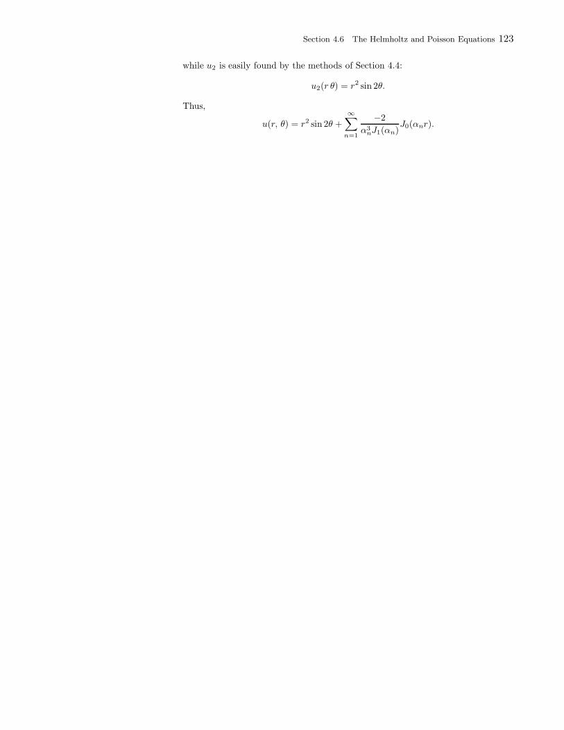
Section 4.6 The Helmholtz and Poisson Equations 123
while u2 is easily found by the methods of Section 4.4:
u2(r θ) = r2 sin 2θ.
Thus,
u(r, θ) = r2 sin 2θ +
∞∑
n=1
−2
α3nJ1(αn)
J0(αnr).
124 Chapter 4 Partial Differential Equations in Polar and Cylindrical Coordinates
Solutions to Exercises 4.7
1. Bessel equation of order 3. Using (7), the first series solution is
J3(x) =
∞∑
k=0
(−1)k
k!(k+ 3)!
(x2
)2k+3
=1
1 · 6x3
8− 1
1 · 24
x5
32+
1
2 · 120
x7
128+ · · · .
5. Bessel equation of order 32. The general solution is
y(x) = c1J 32
+ c2J− 32
= c1
(1
1 · Γ(52)
(x2
) 32 − 1
1 · Γ(72 )
(x2
) 72
+ · · ·)
+c2
(1
1 · Γ(−12
)
(x2
)− 32 − 1
1 · Γ(12)
(x2
) 12
+ · · ·).
Using the basic property of the gamma function and (15), we have
Γ(52 ) = 3
2Γ(32) = 3
212Γ(1
2) = 34
√π
Γ(72) = 5
2Γ(52 ) = 15
8
√π
−12Γ(−1
2) = Γ(1
2) =
√π ⇒ Γ(−1
2) = −2
√π.
So
y(x) = c1
√2
πx
(4
3
x2
4− 8
15
x4
16+ · · ·
)
c2
√2
πx(−1)
(−1
2
2
x− x
2− · · ·
)
= c1
√2
πx
(x2
3− x4
30+ · · ·
)+ c2
√2
πx
(1
x+x
2− · · ·
)
9. Divide the equation through by x2 and put it in the form
y′′ +1
xy′ +
x2 − 9
x2y = 0 for x > 0.
Now refer to Appendix A.6 for terminology and for the method of Frobenius thatwe are about to use in this exercise. Let
p(x) =1
xfor q(x) =
x2 − 9
x2.
The point x = 0 is a singular point of the equation. But since x p(x) = 1 andx2 q(x) = x2 − 9 have power series expansions about 0 (in fact, they are alreadygiven by their power series expansions), it follows that x = 0 is a regular singularpoint. Hence we may apply the Frobenius method. We have already found oneseries solution in Exercise 1. To determine the second series solution, we considerthe indicial equation
r(r − 1) + p0r + q0 = 0,
where p0 = 1 and q0 = −9 (respectively, these are the constant terms in the seriesexpansions of xp(x) and x2q(x)). Thus the indicial equation is
r − 9 = 0 ⇒ r1 = 3, r2 = −3.
The indicial roots differ by an integer. So, according to Theorem 2, Appendix A.6,the second solution y2 may or may not contain a logarithmic term. We have, forx > 0,
y2 = ky1 lnx+ x−3∞∑
m=0
bmxm = ky1 lnx+
∞∑
m=0
bmxm−3,
Section 4.7 Bessel’s Equation and Bessel Functions 125
where a0 6= 0 and b0 6= 0, and k may or may not be 0. Plugging this into thedifferential equation
x2y′′ + xy′ + (x2 − 9)y = 0
and using the fact that y1 is a solution, we have
y2 = ky1 lnx+
∞∑
m=0
bmxm−3
y′2 = ky′1 lnx+ ky1x
+
∞∑
m=0
(m− 3)bmxm−4;
y′′2 = ky′′1 lnx+ ky′1x
+ kxy′1 − y1
x2+
∞∑
m=0
(m− 3)(m− 4)bmxm−5
= ky′′1 lnx+ 2ky′1x
− ky1x2
+
∞∑
m=0
(m− 3)(m− 4)bmxm−5;
x2y′′2 + xy′2 + (x2 − 9)y2
= kx2y′′1 lnx+ 2kxy′1 − ky1 +
∞∑
m=0
(m− 3)(m− 4)bmxm−3
+kxy′1 lnx+ ky1 +∞∑
m=0
(m− 3)bmxm−3
+(x2 − 9)
[ky1 lnx+
∞∑
m=0
bmxm−3
]
= k lnx[
=0︷ ︸︸ ︷x2y′′1 + xy′1 + (x2 − 9)y1
]
+2kxy′1 +
∞∑
m=0
[(m− 3)(m− 4)bm + (m− 3)bm − 9bm
]xm−3
+x2∞∑
m=0
bmxm−3
= 2kxy′1 +
∞∑
m=0
(m− 6)mbmxm−3 +
∞∑
m=0
bmxm−1.
To combine the last two series, we use reindexing as follows
∞∑
m=0
(m− 6)mbmxm−3 +
∞∑
m=0
bmxm−1
= −5b1x−2 +
∞∑
m=2
(m− 6)mbmxm−3 +
∞∑
m=2
bm−2xm−3
= −5b1x−2 +
∞∑
m=2
[(m− 6)mbm + bm−2
]xm−3.
Thus the equationx2y′′2 + xy′2 + (x2 − 9)y2 = 0
implies that
2kxy′1 − 5b1x−2 +
∞∑
m=2
[(m− 6)mbm + bm−2
]xm−3 = 0.
126 Chapter 4 Partial Differential Equations in Polar and Cylindrical Coordinates
This equation determines the coefficients bm (m ≥ 1) in terms of the coefficients ofy1. Furthermore, it will become apparent that k cannot be 0. Also, b0 is arbitrarybut by assumption b0 6= 0. Let’s take b0 = 1 and determine the the first five bm’s.
Recall from Exercise 1
y1 =1
1 · 6x3
8− 1
1 · 24
x5
32+
1
2 · 120
x7
128+ · · · .
So
y′1 =3
1 · 6x2
8− 5
1 · 24
x4
32+
7
2 · 120
x6
128+ · · ·
and hence (taking k = 1)
2kxy′1 =6k
1 · 6x3
8− 10k
1 · 24
x5
32+
14k
2 · 120
x7
128+ · · · .
The lowest exponent of x in
2kxy′1 − 5b1x−2 +
∞∑
m=2
[(m− 6)mbm + bm−2
]xm−3
is x−2. Since its coefficient is −5b1, we get b1 = 0 and the equation becomes
2xy′1 +
∞∑
m=2
[(m− 6)mbm + bm−2
]xm−3.
Next, we consider the coefficient of x−1. It is (−4)2b2 + b0. Setting it equal to 0,we find
b2 =b08
=1
8.
Next, we consider the constant term, which is the m = 3 term in the series. Settingits coefficient equal to 0, we obtain
(−3)3b3 + b1 = 0 ⇒ b3 = 0
because b1 = 0. Next, we consider the term in x, which is the m = 4 term in theseries. Setting its coefficient equal to 0, we obtain
(−2)4b4 + b2 = 0 ⇒ b4 =1
8b2 =
1
64.
Next, we consider the term in x2, which is the m = 5 term in the series. Setting itscoefficient equal to 0, we obtain b5 = 0. Next, we consider the term in x3, whichis the m = 6 term in the series plus the first term in 2kxy′1. Setting its coefficientequal to 0, we obtain
0 + b4 +k
8= 0 ⇒ k = −8b4 = −1
8.
Next, we consider the term in x4, which is the m = 7 term in the series. Settingits coefficient equal to 0, we find that b7 = 0. It is clear that b2m+1 = 0 and that
y2 ≈ −1
8y1 lnx+
1
x3+
1
8 x+
1
64x+ · · ·
Any nonzero constant multiple of y2 is also a second linearly independent solutionof y1. In particular, 384 y2 is an alternative answer (which is the answer given inthe text).
11. The equation is of the form given in Exercise 10 with p = 0. Thus its generalsolution is
y = c1J0(x) + c2Y0(x).
Section 4.7 Bessel’s Equation and Bessel Functions 127
This is, of course, the general solution of Bessel’s equation of order 0. Indeed, thegiven equation is equivalent to Bessel’s equation of order 0.
13. The equation is of the form given in Exercise 10 with p = 3/2. Thus its generalsolution is
y = c1x3/2J3/2(x) + c2x
3/2Y3/2(x).
Using Exercise 22 and (1), you can also write this general solution in the form
y = c1x
[sinx
x− cosx
]+ c2x
[−cosx
x− sinx
]
= c1 [sinx− x cosx] + c2 [− cos x− x sinx] .
In particular, two linearly independent solution are
y1 = sinx− x cosx and y2 = cosx+ x sinx.
This can be verified directly by using the differential equation (try it!).
15. All three parts, (a)–(c), follow directly from the series form of Jp(x) (see (7)).
17. We have
y = x−pu,
y′ = −px−p−1u+ x−pu′,
y′′ = p(p+ 1)x−p−2u+ 2(−p)x−p−1u′ + x−pu′′,
xy′′ + (1 + 2p)y′ + xy = x[p(p+ 1)x−p−2u− 2px−p−1u′ + x−pu′′
]
+(1 + 2p)[− px−p−1u+ x−pu′
]+ x x−pu
= x−p−1[x2u′′ + [−2px+ (1 + 2p)x]u′
+[p(p+ 1) − (1 + 2p)p+ x2]u]
= x−p−1[x2u′′ + xu′ + (x2 − p2)u
].
Thus, by letting y = x−pu, we transform the equation
xy′′ + (1 + 2p)y′ + xy = 0
into the equation
x−p−1[x2u′′ + xu′ + (x2 − p2)u
]= 0,
which, for x > 0, is equivalent to
x2u′′ + xu′ + (x2 − p2)u = 0,
a Bessel equation of ordr p > 0 in u. The general solution of the last equation is
u = c1Jp(x) + c2Yp(x).
Thus the general solution of the original equation is
Y = c1x−pJp(x) + c2x
−pYp(x).
128 Chapter 4 Partial Differential Equations in Polar and Cylindrical Coordinates
21. Using (7),
J− 12(x) =
∞∑
k=0
(−1)k
k!Γ(k − 12
+ 1)
(x2
)2k−12
=
√2
x
∞∑
k=0
(−1)k
k!Γ(k + 12 )
x2k
22k
=
√2
x
∞∑
k=0
(−1)k
k!
22kk!
(2k)!√π
x2k
22k(by Exercise 44(a))
=
√2
π x
∞∑
k=0
(−1)k
k!
x2k
(2k)!=
√2
π xcosx.
22. (a) Using (7),
J 32(x) =
∞∑
k=0
(−1)k
k!Γ(k+ 32 + 1)
(x2
)2k+32
=
√2
x
∞∑
k=0
(−1)k
k!Γ(k+ 2 + 12 )
x2k+2
22k+2
=
√2
πx
∞∑
k=0
(−1)k
k!
2 22k+1k!
(2k + 3)(2k + 1)!
x2k+2
22k+2
(Γ(k + 2 +1
2) = Γ(k + 1 +
1
2)Γ(k + 1 +
1
2) then use Exercise 44(b))
=
√2
π x
∞∑
k=0
(−1)k(2k + 2)
(2k + 3)!x2k+2 (multiply and divide by (2k + 2))
=
√2
π x
∞∑
k=1
(−1)k−1(2k)
(2k + 1)!x2k (change k to k − 1)
=
√2
π x
∞∑
k=1
(−1)k−1[(2k + 1) − 1]
(2k + 1)!x2k
=
√2
π x
∞∑
k=1
(−1)k−1
(2k)!x2k −
√2
π x
∞∑
k=1
(−1)k−1
(2k + 1)!x2k
=
√2
π x
(− cos x+
sinx
x
).
25. (a) Let u = 2a e
− 12 (at−b), Y (u) = y(t), e−at+b = a2
4 u2; then
dy
dt=dY
du
du
dt= Y ′ (−e− 1
2 (at−b));d2y
dt2=
d
du
(Y ′ (−e− 1
2 (at−b)))
= Y ′′e−at+b+Y ′a
2e−
12 (at−b).
So
Y ′′e−at+b + Y ′ a
2e−
12 (at−b) + Y e−at+b = 0 ⇒ Y ′′ +
a
2Y ′e−
12 (at−b) + Y = 0,
upon multiplying by eat−b. Using u = 2ae−
12 (at−b), we get
Y ′′ +1
uY ′ + Y = 0 ⇒ u2Y ′′ + uY ′ + u2Y = 0,
which is Bessel’s equation of order 0.(b) The general solution of u2Y ′′ + uY ′ + u2Y = 0 is Y (u) = c1J0(u) + c2Y0(u).
But Y (u) = y(t) and u = 2ae−
12 (at−b), so
y(t) = c1J0(2
ae−
12 (at−b)) + c2Y0(
2
ae−
12 (at−b)).
Section 4.7 Bessel’s Equation and Bessel Functions 129
(c) (i) If c1 = 0 and c2 6= 0, then
y(t) = c2Y0(2
ae−
12 (at−b)).
As t → ∞, u→ 0, and Y0(u) → −∞. In this case, y(t) could approach either +∞or −∞ depending on the sign of c2. y(t) would approach infinity linearly as near
0, Y0(x) ≈ lnx so y(t) ≈ ln(
2ae−
12 (at−b)
)≈ At.
(ii) If c1 6= 0 and c2 = 0, then
y(t) = c1J0(2
ae−
12 (at−b)).
As t → ∞, u(t) → 0, J0(u) → 1, and y(t) → c1. In this case the solution isbounded.(ii) If c1 6= 0 and c2 6= 0, as t → ∞, u(t) → 0, J0(u) → 1, Y0(u) → −∞. Since Y0
will dominate, the solution will behave like case (i).It makes sense to have unbounded solutions because eventually the spring wears
out and does not affect the motion. Newton’s laws tell us the mass will continuewith unperturbed momentum, i.e., as t → ∞, y′′ = 0 and so y(t) = c1t + c2, alinear function, which is unbounded if c1 6= 0.
31. (a) From Γ(x) =∫∞0tx−1e−t dt, we obtain
Γ(1) =
∫ ∞
0
e−t dt = −e−t
∣∣∣∣∞
0
= 1;
Γ(2) =
∫ ∞
0
te−t dt =
=0︷ ︸︸ ︷−te−t
∣∣∣∞
0+
∫ ∞
0
e−t dt = 1.
(b) Using (15) and the basic property of the gamma function
Γ(52) = 3
2Γ(3
2) = 3
212Γ(1
2) = 3
4
√π
−32Γ(−3
2 ) = Γ(−12) = −2
√π (see Exercise 5) ⇒ Γ(−3
2) = 43
√π.
33. (a) In (13), let u2 = t, 2u du = dt, then
Γ(x) =
∫ ∞
0
tx−1e−t dt =
∫ ∞
0
u2(x−1)e−u2
(2u)du = 2
∫ ∞
0
u2x−1e−u2
du.
(b) Using (a)
Γ(x)Γ(y) = 2
∫ ∞
0
u2x−1e−u2
du2
∫ ∞
0
v2y−1e−v2
dv
= 4
∫ ∞
0
∫ ∞
0
e−(u2+v2)u2x−1v2y−1du dv.
(c) Switching to polar coordinates: u = r cos θ, v = r sin θ, u2 + v2 = r2, dudv =rdrdθ; for (u, v) varying in the first quadrant (0 ≤ u < ∞ and 0 ≤ v < ∞), wehave 0 ≤ θ ≤ π
2 , and 0 ≤ r <∞, and the double integral in (b) becomes
Γ(x)Γ(y) = 4
∫ ∞
0
∫ π2
0
e−r2
(r cos θ)2x−1(r sin θ)2y−1rdrdθ
= 2
∫ π2
0
(cos θ)2x−1(sin θ)2y−1dθ
=Γ(x+y)︷ ︸︸ ︷2
∫ ∞
0
r2(x+y)−1e−r2
dr
(use (a) with x+ y in place of x)
= 2Γ(x+ y)
∫ π2
0
(cos θ)2x−1(sin θ)2y−1dθ,
130 Chapter 4 Partial Differential Equations in Polar and Cylindrical Coordinates
implying (c).
41. Let I =∫ π/2
0sin2k+1 θ dθ. Applying Exercise 33, we take 2x− 1 = 0 and
2y − 1 = 2k + 1, so x = 12 and y = k + 1. Then
2I =Γ(1
2) Γ(k + 1)
Γ(k + 1 + 12)
=
√π k!
(k + 12)Γ(k + 1
2 )=
2√π k!
(2k + 1)Γ(k + 12 ).
As in (a), we now use Γ(k + 12 ) = (2k)!
22kk!
√π, simplify, and get
I =22k(k!)2
(2k + 1)!.
Section 4.8 Bessel Series Expansions 131
Solutions to Exercises 4.8
1. (a) Using the series definition of the Bessel function, (7), Section 4.7, we have
d
dx[x−pJp(x)] =
d
dx
∞∑
k=0
(−1)k
2pk!Γ(k + p+ 1)
(x2
)2k
=
∞∑
k=0
(−1)k
2pk!Γ(k + p+ 1)
d
dx
(x2
)2k
=
∞∑
k=0
(−1)k2k
2pk!Γ(k+ p+ 1)
1
2
(x2
)2k−1
=∞∑
k=0
(−1)k
2p(k − 1)!Γ(k+ p+ 1)
(x2
)2k−1
= −∞∑
m=0
(−1)m
2pm!Γ(m+ p+ 2)
(x2
)2m+1
(set m = k − 1)
= −x−p∞∑
m=0
(−1)m
m!Γ(m+ p + 2)
(x2
)2m+p+1
= −x−pJp+1(x).
To prove (7), use (1):
d
dx[xpJp(x)] = xpJp−1(x) ⇒
∫xpJp−1(x) dx = xpJp(x) +C.
Now replace p by p+ 1 and get
∫xp+1Jp(x) dx = xp+1Jp+1(x) + C,
which is (7). Similarly, starting with (2),
d
dx[x−pJp(x)] = −x−pJp+1(x) ⇒ −
∫x−pJp+1(x) dx = x−pJp(x) +C
⇒∫x−pJp+1(x) dx = −x−pJp(x) +C.
Now replace p by p− 1 and get
∫x−p+1Jp(x) dx = −x−p+1Jp−1(x) +C,
which is (8).(b) To prove (4), carry out the differentiation in (2) to obtain
x−pJ ′p(x) − px−p−1Jp(x) = −x−pJp+1(x) ⇒ xJ ′
p(x) − pJp(x) = −xJp+1(x),
upon multiplying through by xp+1. To prove (5), add (3) and (4) and then divideby x to obtain
Jp−1(x) − Jp+1(x) = 2J ′p(x).
To prove (6), subtract (4) from (3) then divide by x.
3.
∫xJ0(x) dx = xJ1(x) + C, by (7) with p = 0.
5.
∫J1(x) dx = −J0(x) + C, by (8) with p = 1.
7.
∫x3J2(x) dx = x3J3(x) +C, by (7) with p = 2.
132 Chapter 4 Partial Differential Equations in Polar and Cylindrical Coordinates
9.∫J3(x) dx =
∫x2[x−2J3(x)] dx
x2 = u, x−2J3(x) dx = dv, 2x dx = du, v = −x−2J2(x)
= −J2(x) + 2
∫x−1J2(x) dx = −J2(x) − 2x−1J1(x) + C
= J0(x) −2
xJ1(x) −
2
xJ1(x) +C(use (6) with p = 1)
= J0(x) −4
xJ1(x) + C.
11. By (2) with p = 12,
J3/2(x) = −x 12d
dx
[x−
12 J 1
2(x)]
= −x 12
√2
π
d
dx
(sinx
x
)
= −√
2
πx
12
(cos x
x− sinx
x2
)=
√2
π x
(sinx
x− cosx
).
13. Use (6) with p = 4. Then
J5(x) =8
xJ4(x) − J3(x)
=8
x
[6
xJ3(x) − J2(x)
]− J3(x) (by (6) with p = 3)
=
(48
x2− 1
)J3(x) −
8
xJ2(x)
=
(48
x2− 1
)(4
xJ2(x) − J1(x)
)− 8
xJ2(x) (by (6) with p = 2)
=
(192
x3− 12
x
)J2(x) −
(48
x2− 1
)J1(x)
=12
x
(16
x2− 1
)[2
xJ1(x) − J0(x)
]−(
48
x2− 1
)J1(x)
(by (6) with p = 1)
= −12
x
(16
x2− 1
)J0(x) +
(384
x4− 72
x2+ 1
)J1(x).
15. (a) and (b) We will do this problem on Mathematica. Let us make somecomments about the equation sin x
x = cos x. This equation is equivalent to theequation tanx = x, which we have encountered in Section 3.6. It is clear fromthe graph that this equation has one root xk in each interval
(−π
2+ kπ, π
2+ kπ
),
k = 0, 1, 2, . . .. We have x0 = 0 and the remaininng roots can be obtained byiteration as follows. Take the case k = 1. Start at z1 = π and go up to the liney = x then over to the right to the graph of tanx. You will intersect this graph atthe point z2 = π + tan−1 π. Repeat hese steps by going up to the line y = x andthen over to the right to the graph of y = tanx. You will intersect the graph atz2 = π+ tan−1 z1. As you continue this process, you will approach the value of x1.To find xk, start at z1 = kπ and construct the sequence zn = kπ+tan−1 zn−1. Letus compute some numerical values and then compare them with the roots that wefind by using built-in commands from Mathematica.
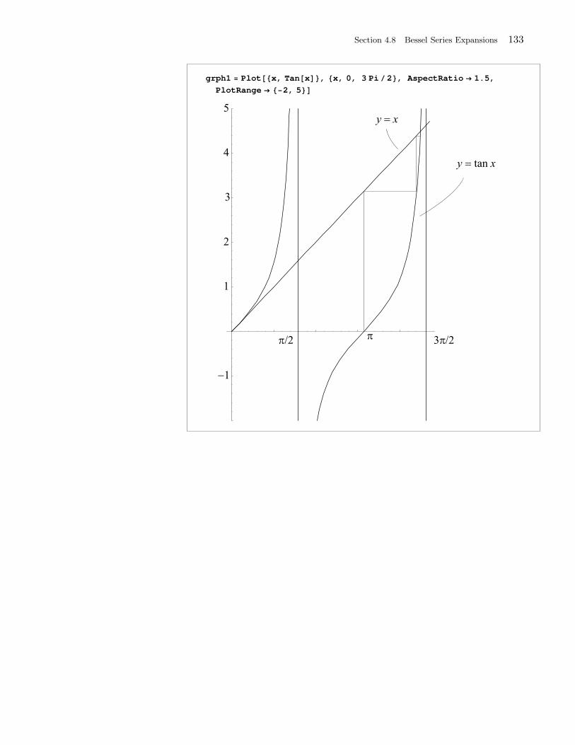
Section 4.8 Bessel Series Expansions 133
grph1 Plot x, Tan x , x, 0, 3 Pi 2 , AspectRatio 1.5,
PlotRange 2, 5
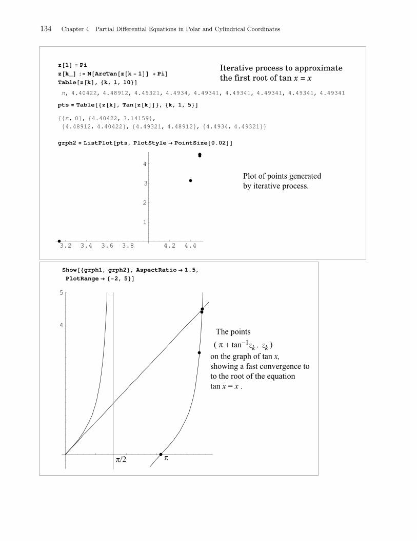
134 Chapter 4 Partial Differential Equations in Polar and Cylindrical Coordinates
z 1 Pi
z k_ : N ArcTan z k 1 Pi
Table z k , k, 1, 10
, 4.40422, 4.48912, 4.49321, 4.4934, 4.49341, 4.49341, 4.49341, 4.49341, 4.49341
pts Table z k , Tan z k , k, 1, 5
, 0 , 4.40422, 3.14159 ,
4.48912, 4.40422 , 4.49321, 4.48912 , 4.4934, 4.49321
grph2 ListPlot pts, PlotStyle PointSize 0.02
3.2 3.4 3.6 3.8 4.2 4.4
1
2
3
4
Iterative process to approximate
the first root of tan x = x
Show grph1, grph2 , AspectRatio 1.5,
PlotRange 2, 5
4
5
tan zk
, zk
Section 4.8 Bessel Series Expansions 135
If you want to use a built-in command to find the root, you can do the following(compare the result with the iterative process above).
FindRoot Tan x x, x, 4
x 4.49341
17. (a) From (17),
Aj =2
J1(αj)2
∫ 1
0
f(x)J0(αjx)x dx =2
J1(αj)2
∫ c
0
J0(αjx)x dx
=2
α2jJ1(αj)2
∫ cαj
0
J0(s)s ds (let αjx = s)
=2
α2jJ1(αj)2
J1(s)s
∣∣∣∣∣
cαj
0
=2cJ1(αj)
αjJ1(αj)2.
Thus, for 0 < x < 1,
f(x) =
∞∑
j=1
2cJ1(αj)
αjJ1(αj)2J0(αjx).
(b) The function f is piecewise smooth, so by Theorem 2 the series in (a) convergesto f(x) for all 0 < x < 1, except at x = c, where the series converges to the average
value f(c+)+f(c−)2 = 1
2 .
19. (a) This is a Bessel series of order 4. By Theorem 2, we have
Aj =2
J5(α4,j)2
∫ 1
0
x4J4(α4,jx)x dx
=2
α64,jJ1(α4,j)2
∫ α4,j
0
J4(s)s5 ds (let α4,jx = s)
=2
α64,jJ5(α4,j)2
J5(s)s5
∣∣∣∣∣
α4,j
0
=2
α4,jJ5(α4,j).
Thus, for 0 < x < 1,
x4 = 2
∞∑
j=1
J4(α4,jx)
α4,jJ5(α4,j).
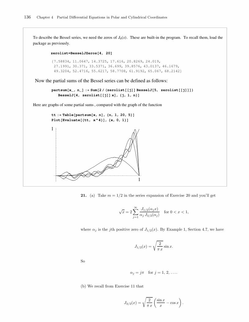
136 Chapter 4 Partial Differential Equations in Polar and Cylindrical Coordinates
To describe the Bessel series, we need the zeros of J0 x . These are built-in the program. To recall them, load the
package as previously.
zerolist=BesselJZeros[4, 20]
7.58834, 11.0647, 14.3725, 17.616, 20.8269, 24.019,
27.1991, 30.371, 33.5371, 36.699, 39.8576, 43.0137, 46.1679,
49.3204, 52.4716, 55.6217, 58.7708, 61.9192, 65.067, 68.2142
Now the partial sums of the Bessel series can be defined as follows:
partsum x_, n_ : Sum 2 zerolist j BesselJ 5, zerolist j
BesselJ 4, zerolist j x , j, 1, n
Here are graphs of some partial sums , compared with the graph of the function
tt : Table partsum x, n , n, 1, 20, 5
Plot Evaluate tt, x^4 , x, 0, 1
21. (a) Take m = 1/2 in the series expansion of Exercise 20 and you’ll get
√x = 2
∞∑
j=1
J1/2(αjx)
αj J3/2(αj)for 0 < x < 1,
where αj is the jth positive zero of J1/2(x). By Example 1, Section 4.7, we have
J1/2(x) =
√2
π xsinx.
So
αj = jπ for j = 1, 2, . . . .
(b) We recall from Exercise 11 that
J3/2(x) =
√2
π x
(sinx
x− cos x
).
Section 4.8 Bessel Series Expansions 137
So the coefficients are
Aj =2
αj J3/2(αj)=
2
jπ J3/2(jπ)
=2
jπ√
2π jπ
(sin jπ
jπ − cos jπ)
= (−1)j−1
√2
j
and the Bessel series expansion becomes, or 0 < x < 1,
√x =
∞∑
j=1
(−1)j−1
√2
jJ1/2(αjx).
(c) Writing J1/2(x) in terms of sinx and simplifying, this expansion becomes
√x =
∞∑
j=1
(−1)j−1
√2
jJ1/2(αjx)
=
∞∑
j=1
(−1)j−1
√2
j
√2
π αjsinαj
=2
π
∞∑
j=1
(−1)j−1
j
sin(jπx)√x
.
Upon multiplying both sides by√x, we obtain
x =2
π
∞∑
j=1
(−1)j−1
jsin(jπx) for 0 < x < 1,
which is the familiar Fourier sine series (half-range expansion) of the functionf(x) = x.
23. Just repeat the computation in Exercises 20 with m = 2 and you will get, for0 < x < 1,
x2 = 2
∞∑
j=1
1
α2,jJ3(α2,j)J2(α2,jx).
25. By Theorem 2 with p = 1, we have
Aj =2
J2(α1,j)2
∫ 1
12
J1(α1,jx) dx
=2
α1,jJ2(α1,j)2
∫ α1,j
α1,j2
J1(s) ds (let α1,jx = s)
=2
α1,jJ2(α1,j)2[−J0(s)
∣∣∣∣α1,j
α1,j2
(by (8) with p = 1)
=−2[J0(α1,j) − J0(
α1,j
2)]
α1,jJ2(α1,j)2
=−2[J0(α1,j) − J0(
α1,j
2)]
α1,jJ0(α1,j)2,
138 Chapter 4 Partial Differential Equations in Polar and Cylindrical Coordinates
where in the last equality we used (6) with p = 1 at x = α1,j (so J0(α1,j)+J2(α1,j) =0 or J0(α1,j) = −J2(α1,j)). Thus, for 0 < x < 1,
f(x) = −2
∞∑
j=1
−2[J0(α1,j) − J0(
α1,j
2 )]
α1,jJ0(α1,j)2J1(α1,jx).
27. By Theorem 2 with p = 2, we have
Aj =2
J3(α2,j)2
∫ 1
12
x−1J2(α2,jx) dx
=2
J3(α2,j)2
∫ α2,j
α2,j2
J2(s)s−1 ds (let α2,jx = s)
=2
J3(α2,j)2[−s−1J1(s)
∣∣∣∣α2,j
α2,j2
=2
J1(α2,j)2
[−J1(α2,j)
α2,j+ 2
J1
(α2,j
2
)
α2,j
]
(because J3 = −J1 at a zero of J2 by (6))
=−2[J1(α2,j) − 2J1(
α2,j
2 )]
α2,jJ1(α2,j)2.
Thus, for 0 < x < 1,
f(x) = −2
∞∑
j=1
J1(α2,j) − 2J1(α2,j
2 )
α2,jJ1(α2,j)2J2(α2,jx).
29. By Theorem 2 with p = 1, we have
Aj =1
2 J2(α1,j)2
∫ 2
0
J1(α2,jx/2)x dx
=2
α21,jJ2(α1,j)2
∫ α1,j
0
J1(s)s ds (let α1,jx/2 = s).
Since we cannot evaluate the definite integral in a simpler form, just leave it as itis and write the Bessel series expansion as
1 =∞∑
j=1
2
α21,jJ2(α1,j)2
[∫ α1,j
0
J1(s)s ds
]J1(α1,jx/2) for 0 < x < 2.
31. p = 1, y = c1J1(λx) + c2Y1(λx). For y to be bounded near 0, we musttake c2 = 0. For y(1) = 0, we must take λ = λj = α1,j, j = 1, 2, . . .; and soy = yi = c1,jJ1(α1,jx).
33. p = 12 , y = c1J 1
2(λx) + c2Y 1
2(λx). For y to be bounded near 0, we must
take c2 = 0. For y(π) = 0, we must take λ = λj =α 1
2,j
π = j, j = 1, 2, . . . (seeExercises 21); and so
y = yi = c1,jJ1(α 1
2 ,j
πx) = c1,j
√2
πxsin(jx)
(see Example 1, Section 4.7).
35. (b) Bessel’s equation of order 0 is xy′′ + y′ + xy = 0. Take y = x−12u. Then
y′ = x−12 [u′ − 1
2xu] and
y′′ = x−12 [u′′ − 1
2xu′ +
1
2x2u− 1
2x
(u′ − 1
2xu)]
= x−12 [u′′ − 1
xu′ +
3
4x2u].
Section 4.8 Bessel Series Expansions 139
Substituting into Bessel’s equation and simplifying, we find
(xu′′ − u′ +
3
4xu)
+(u′ − 1
2xu)
+ xu = 0 ⇒ u′′ +(1 +
1
4x2
)u = 0 (∗).
Since J0(x) satisfies Bessel’s equation, it follows that u =√xJ0(x) is a solution of
the last displayed equation (∗).(c) Let v = sinx. Then v′′ + v = 0. Multiplying this equation by u and (∗) by v,and then subtracting yields
uv′′ − vu′′ =1
4x2uv ⇒
(uv′ − u′v
)′=
1
4x2uv,
which implies (c), since 14x2uv = −(u′′ + u)v from (b) (multiply the displayed
equation in (b) by v).(d) is clear from (b).(e) Integrating both sides of the equation
(uv′ − u′v
)′=
1
4x2uv
from (c), we obtain ∫1
4x2uv dx = uv′ − u′v +C.
So for any positive integer k,
∫ (2k+1)π
2kπ
1
4x2u(x) sinx dx = uv′ − u′v
∣∣∣(2k+1)π
2kπ= u cosx− u′ sinx
∣∣∣(2k+1)π
2kπ
= −(u(2kπ) + u((2k + 1)π)
).
(f) Consider the integrand in (e), u(x) sin x4x2 . This is a continuous function on
[2kπ, (2k + 1)π]. We have sin x4x2 > 0 for all x in (2kπ, (2k + 1)π), because sinx > 0
for all x in (2kπ, (2k+1)π). Assume that u(x) does not vanish in (2kπ, (2k+1)π).So u(x) > 0 or u(x) < 0 for all x in (2kπ, (2k + 1)π). Take the case u(x) > 0 for
all x in (2kπ, (2k + 1)π). Then u(x) sin x4x2 > 0 for all x in (2kπ, (2k + 1)π), which
implies that ∫ (2k+1)π
2kπ
u(x) sinx
4x2dx > 0.
By continuity of u, it follows that u(2kπ) ≥ 0 and u((2k + 1)π) ≥ 0, and so (e)implies that ∫ (2k+1)π
2kπ
u(x) sinx
4x2dx ≤ 0,
which is a contradiction. Thus u(x) is not positive for all x in (2kπ, (2k+1)π) andso it must vanish at some point inside this interval. A similar argument shows thatu(x) cannot be negative for all x in (2kπ, (2k + 1)π), and thus u must vanish atsome point in (2kπ, (2k + 1)π).(g) From (f) it follows that u has infinitely many zeros on the positive real line; atleast one in each interval of the form (2kπ, (2k + 1)π). Since these intervals aredisjoint, these zeros are distinct. Now J0 and u have the same zeros, and so thesame applies to the zeros of J0.
Note: You can repeat the above proof with sinx replaced by sin(x−a) and showthat u (and hence J0) has at least one zero in every interval of the form (a, a+ π)for any a > 0.
One more formula. To complement the integral formulas from this section,consider the following interesting formula. Let a, b, c, and p be positive real numberswith a 6= b. Then
∫ c
0
Jp(ax)Jp(bx)x dx =c
b2 − a2
[aJp(bc)Jp−1(ac) − bJp(ac)Jp−1(bc)
].
140 Chapter 4 Partial Differential Equations in Polar and Cylindrical Coordinates
To prove this formula, we note that y1 = Jp(ax) satisfies
x2y′′1 + xy′1 + (a2x2 − p2)y1 = 0
and y2 = Jp(bx) satisfies
x2y′′2 + xy′2 + (b2x2 − p2)y2 = 0.
Write these equations in the form
(xy′1)′
+ y′1 +a2x2 − p2
xy1 = 0
and(xy′2)′
+ y′2 +b2x2 − p2
xy1 = 0.
Multiply the first by y2 and the second by y − 1, subtract, simplify, and get
y2(xy′1)′ − y1
(xy′2)′
= y1y2(b2 − a2)x.
Note that
y2(xy′1)′ − y1
(xy′2)′
=d
dx
[y2(xy
′1) − y1(xy
′2)].
So
(b2 − a2)y1y2x =d
dx
[y2(xy
′1) − y1(xy
′2)],
and, after integrating,
(b2 − a2)
∫ c
0
y1(x)y2(x)x dx =[y2(xy
′1) − y1(xy
′2)]∣∣∣
c
0= x
[y2y
′1 − y1y
′2
]∣∣∣c
0.
On the left, we have the desired integral times (b2 − a2) and, on the right, we have
c[Jp(bc)aJ
′p(ac) − bJp(ac)J
′p(bc)
]− c[aJp(0)J ′
p(0) − bJp(0)J ′p(0)
].
Since Jp(0) = 0 if p > 0 and J ′0(x) = −J1(x), it follows that Jp(0)J ′
p(0) −Jp(0)J ′
p(0) = 0 for all p > 0. Hence the integral is equal to
I =
∫ c
0
Jp(ax)Jp(bx)x dx =c
b2 − a2
[aJp(bc)J
′p(ac) − bJp(ac)J
′p(bc)
].
Now using the formula
J ′p(x) =
1
2
[Jp−1(x) − Jp+1(x)
],
we obtain
I =c
2(b2 − a2)
[aJp(bc)
(Jp−1(ac) − Jp+1(ac)
)− bJp(ac)
(Jp−1(bc) − Jp+1(bc)
)].
Simplify with the help of the formula
Jp+1(x) =2p
xJp(x) − Jp−1(x)
and you get
I =c
2(b2 − a2)
[aJp(bc)
(Jp−1(ac) − (
2p
acJp(ac) − Jp−1(ac))
)
−bJp(ac)(Jp−1(bc) − (
2p
bcJp(bc) − Jp−1(bc))
)]
=c
b2 − a2
[aJp(bc)Jp−1(ac) − bJp(ac)Jp−1(bc)
],
as claimed.Note that this formula implies the orthogonality of Bessel functions. In fact its
proof mirrors the proof of orthogonality from Section 4.8.
Section 4.9 Integral Formulas and Asymptotics for Bessel Functions 141
Solutions to Exercises 4.9
1. We have
J0(x) =1
π
∫ π
0
cos(− x sin θ
)dθ =
1
π
∫ π
0
cos(x sin θ
)dθ.
So
J0(0) =1
π
∫ π
0
dθ = 1.
For n 6= 0,
Jn(x) =1
π
∫ π
0
cos(nθ − x sin θ
)dθ;
so
Jn(0) =1
π
∫ π
0
cos nθ dθ = 0.
3. taking imaginary parts from teh series in Exampe 2, we obtain
sinx =
∞∑
n=−∞Jn(x) sin
nπ
2
=
∞∑
n=1
Jn(x) sinnπ
2+
n=−∞∑
−1
Jn(x) sinnπ
2
=
∞∑
n=1
Jn(x) sinnπ
2−
∞∑
n=1
J−n(x) sin(nπ
2
)
=
∞∑
k=0
J2k+1(x)(−1)k −∞∑
k=0
J−(2k+1)(x)
= 2
∞∑
k=0
(−1)kJ2k+1(x).
5. All the terms in the series
1 = J0(x)2 + 2
∞∑
n=1
Jn(x)2
are nonnegative. Since they all add-up to 1, each must be less than or equal to 1.Hence
J0(x)2 ≤ 1 ⇒ |J0(x)| ≤ 1
and, for n ≥ 2,
2Jn(x)2 ≤ 1 ⇒ |Jn(x)| ≤ 1√2.
7. We have f(t) = f(π − t) and g(t) = −g(π − t). So
∫ π
0
f(t)g(t) dt =
∫ π/2
0
f(t)g(t) dt +
∫ π
π/2
f(t)g(t) dt
=
∫ π/2
0
f(t)g(t) dt −∫ 0
π/2
f(π − x)g(π − x) dx (let t = π − x)
=
∫ π/2
0
f(t)g(t) dt −∫ π/2
0
f(x)g(x) dx = 0.
142 Chapter 5 Partial Differential Equations in Spherical Coordinates
Solutions to Exercises 5.11. Start with Laplace’s equation in spherical coordinates
(1)∂2u
∂r2+
2
r
∂u
∂r+
1
r2
(∂2u
∂θ2+ cot θ
∂u
∂θ+ csc2 θ
∂2u
∂φ2
)= 0,
where 0 < r < a, 0 < φ < 2π, and 0 < θ < π. To separate variable, take a productsolution of the form
u(r, θ, φ) = R(r)Θ(θ)Φ(φ) = RΘΦ,
and plug it into (1). We get
R′′ΘΦ +2
rR′ΘΦ +
1
r2
(RΘ′′Φ + cot θRΘ′Φ + csc2 θRΘΦ′′
)= 0.
Divide by RΘΦ and multiply by r2:
r2R′′
R+ 2r
R′
R+
Θ′′
Θ+ cot θ
Θ′
Θ+ csc2 θ
Φ′′
Φ= 0.
Now proceed to separate the variables:
r2R′′
R+ 2r
R′
R= −
(Θ′′
Θ+ cot θ
Θ′
Θ+ csc2 θ
Φ′′
Φ
).
Since the left side is a function of r and the right side is a function of φ and θ, eachside must be constant and the constants must be equal. So
r2R′′
R+ 2r
R′
R= µ
andΘ′′
Θ+ cot θ
Θ′
Θ+ csc2 θ
Φ′′
Φ= −µ.
The equation in R is equivalent to (3). Write the second equation in the form
Θ′′
Θ+ cot θ
Θ′
Θ+ µ = − csc2 θ
Φ′′
Φ;
sin2 θ
(Θ′′
Θ+ cot θ
Θ′
Θ+ µ
)= −Φ′′
Φ.
This separates the variables θ and φ, so each side must be constant and the constantmust be equal. Hence
sin2 θ
(Θ′′
Θ+ cot θ
Θ′
Θ+ µ
)= ν
and
ν = −Φ′′
Φ⇒ Φ′′ + νΦ = 0.
We expect 2π-periodic solutions in Φ, because φ is and azimuthal angle. The onlyway for the last equation to have 2π-periodic solutions that are essentially differentis to set ν = m2, where m = 0, 1, 2, . . .. This gives the two equations
Φ′′ +m2Φ = 0
(equation (5)) and
sin2 θ
(Θ′′
Θ+ cot θ
Θ′
Θ+ µ
)= m2,
which is equivalent to (6).
Section 5.1 Preview of Problems and Methods 143
3. From Section 5.5, we have
P0(x) = 1, P1(x) = x, P2(x) =1
2(3x2 − 1).
So
P0(cos θ) = 1, P1(cos θ) = cos θ, P2(cos θ) =1
2(3 cos2 θ − 1).
Next, we verify that these functions are solutions of (7) with µ = n(n + 1), withn = 0, 1, 2, respectively, or µ = 0, 2, 6. (Recall the values of µ from (14).) Forµ = 0, (7) becomes
Θ′′ + cot θΘ′ = 0,
and clearly the constant function P0(cos θ) = 1 is a solution. For µ = 2, (7) becomes
Θ′′ + cot θΘ′ + 2Θ = 0.
Taking Θ = P1(cos θ) = cos θ, we have Θ′ = − sin θ, and Θ′′ = − cos θ. Plugginginto the equation, we find
Θ′′ + cot θΘ′ + 2Θ = − cos θ +cos θ
sin θ(− sin θ) + 2 cos θ = 0.
Finally, for µ = 6, (7) becomes
Θ′′ + cot θΘ′ + 6Θ = 0.
Taking Θ = P2(cos θ) = 12 (3 cos2 θ − 1), we have
Θ′ = −3 sin θ cos θ,
Θ′′ = −3(cos2 θ − sin2 θ
),
Θ′′ + cot θΘ′ + 6Θ = −3(cos2 θ − sin2 θ
)+
cos θ
sin θ(−3 sin θ cos θ)
+3(3 cos2 θ − 1)
= 3(cos2 θ + sin2 θ) − 3 = 0
4. When m = 0, P 01 (cos θ) = P1(cos θ) was treated in Exercise 3. When m = 1,
P 11 (cos θ) = −
√1 − cos2 θ =
√sin2 θ = sin θ. You should note that 0 ≤ θ ≤ π, so
sin θ ≥ 0, thus the positive sign in front of the square root. With m = 1 and µ = 1,equation (6) becomes
Θ′′ + cot θΘ′ + (2 − csc2 θ)Θ = 0.
Taking Θ = P 11 (cos θ) = sin θ, we have Θ′ = cos θ, Θ′′ = − sin θ. So
Θ′′ + cot θΘ′ + (2 − csc2 θ)Θ = − sin θ +cos θ
sin θcos θ +
(2 − 1
sin2 θ
)sin θ
= sin θ +1
sin θ
=− sin2 θ︷ ︸︸ ︷(cos2 θ− 1
)= 0.
144 Chapter 5 Partial Differential Equations in Spherical Coordinates
Solutions to Exercises 5.21. This problem is similar to Example 2. Note that f is its own Legendre series:
f(θ) = 20 (P1(cos θ) + P0(cos θ)).
So really there is no need to compute the Legendre coefficients using integrals. Wesimply have A0 = 20 and A1 = 20, and the solution is
u(r, θ) = 20 + 20 r cos θ.
3. We have
u(r, θ) =∞∑
n=0
AnrnPn(cos θ),
with
An =2n+ 1
2
∫ π
0
f(θ)Pn(cos θ) sin θ dθ
=2n+ 1
2
∫ π2
0
100Pn(cos θ) sin θ dθ +2n+ 1
2
∫ π
π2
20Pn(cos θ) sin θ dθ.
Let x = cos θ, dx = − sin θ dθ. Then
An = 50(2n+ 1)
∫ 1
0
Pn(x) dx+ 10 (2n+ 1)
∫ 0
−1
Pn(x) dx.
The case n = 0 is immediate by using P0(x) = 1,
A0 = 50
∫ 1
0
dx+ 10
∫ 0
−1
dx = 60.
For n > 0, the integrals are not straightforward and you need to refer to Exercise 10,Section 5.6, where they are evaluated. Quoting from this exercise, we have
∫ 1
0
P2n(x)dx = 0, n = 1, 2, . . . ,
and ∫ 1
0
P2n+1(x) dx =(−1)n(2n)!
22n+1(n!)2(n + 1), n = 0, 1, 2, . . . .
Since P2n(x) is an even function, then, for n > 0,
∫ 0
−1
P2n(x) dx =
∫ 1
0
P2n(x) dx = 0.
Hence for n > 0,A2n = 0.
Now P2n+1(x) is an odd function, so
∫ 0
−1
P2n+1(x) dx = −∫ 1
0
P2n+1(x) dx = − (−1)n(2n)!
22n+1(n!)2(n+ 1).
Hence for n = 0, 1, 2, . . .,
A2n+1 = 50(4n+ 3)
∫ 1
0
P2n+1(x) dx+ 10 (4n+ 3)
∫ 0
−1
P2n+1(x) dx
= 50(4n+ 3)(−1)n(2n)!
22n+1(n!)2(n+ 1)− 10 (4n+ 3)
(−1)n(2n)!
22n+1(n!)2(n+ 1)
= 40 (4n+ 3)(−1)n(2n)!
22n+1(n!)2(n + 1)
= 20 (4n+ 3)(−1)n(2n)!
22n(n!)2(n + 1).
Section 5.2 Dirichlet Problems with Symmetry 145
So
u(r, θ) = 60 + 20
∞∑
n=0
(4n+ 3)(−1)n(2n)!
22n(n!)2(n + 1)r2n+1P2n+1(cos θ).
5. Solution We have
u(r, θ) =
∞∑
n=0
AnrnPn(cos θ),
with
An =2n+ 1
2
∫ π
0
f(θ)Pn(cos θ) sin θ dθ
=2n+ 1
2
∫ π2
0
cos θ Pn(cos θ) sin θ dθ
=2n+ 1
2
∫ 1
0
xPn(x) dx,
where, as in Exercise 3, we made the change of variables x = cos θ. At this point,we have to appeal to Exercise 11, Section 5.6, for the evaluation of this integral.(The cases n = 0 and 1 can be done by referring to the explicit formulas for thePn, but we may as well at this point use the full result of Exercise 11, Section 5.6.)We have ∫ 1
0
xP0(x) dx =1
2;
∫ 1
0
xP1(x) dx =1
3;
∫ 1
0
xP2n(x) dx =(−1)n+1(2n− 2)!
22n((n− 1)!)2n(n+ 1); n = 1, 2, . . . ;
and ∫ 1
0
xP2n+1(x) dx = 0; n = 1, 2, . . . .
Thus,
A0 =1
2
1
2=
1
4; A1 =
3
2
1
3=
1
2; A2n+1 = 0, n = 1, 2, 3, . . . ;
and for n = 1, 2, . . .,
A2n =2(2n) + 1
2
(−1)n+1(2n− 2)!
22n((n − 1)!)2n(n + 1)= (4n+ 1)
(−1)n+1(2n− 2)!
22n+1((n− 1)!)2n(n+ 1).
So
u(r, θ) =1
4+
1
2r cos θ +
∞∑
n=1
(−1)n+1(4n+ 1)(2n− 2)!
22n+1((n− 1)!)2n(n+ 1)r2nP2n(cos θ).
7. (a) From (8)
u(r, θ) = 50 + 25
∞∑
n=0
(4n+ 3)(−1)n(2n)!
22n(n!)2(n + 1)r2n+1P2n+1(cos θ) .
Setting θ = π2 , we get
u(r,π
2) = 50 + 25
∞∑
n=0
(4n+ 3)(−1)n(2n)!
22n(n!)2(n+ 1)r2n+1P2n+1(cos
π
2)
= 50 + 25∞∑
n=0
(4n+ 3)(−1)n(2n)!
22n(n!)2(n+ 1)r2n+1
=0︷ ︸︸ ︷P2n+1(0)
= 50
146 Chapter 5 Partial Differential Equations in Spherical Coordinates
This is expected, since the points with θ = π2
are located halfway between theboundary with The temperature at these points is the average value 100+0
2 or 50.(d) For θ = 0, we have
u(r, 0) + u(r, π)
2
= 50 + 25
∞∑
n=0
(4n+ 3)(−1)n(2n)!
22n(n!)2(n+ 1)r2n+1
=0︷ ︸︸ ︷(P2n+1(cos 0) + P2n+1(cosπ))
= 50,
because P2n+1(cos 0) = P2n+1(1) = 1 and P2n+1(cos π) = P2n+1(−1) = −1. Thismakes sense because the average of temperatures equidistant from u = 50 in a ±zsymmetrical environment ought to be 50 itself.9. We first describe the boundary function. From the figure, we see that there isan angle θ0, with cos θ0 = −1
3, and such that
f(θ) =
70 if 0 ≤ θ ≤ θ0,55 if θ0 ≤ θ ≤ π.
Appealing to (5), we have
An =2n+ 1
2
∫ π
0
f(θ)Pn(cos θ) sin θ dθ
=2n+ 1
2
∫ θ0
0
70 cos θ Pn(cos θ) sin θ dθ
+2n+ 1
2
∫ π
θ0
55 cos θ Pn(cos θ) sin θ dθ
=2n+ 1
2
∫ − 13
−1
55Pn(t) dt+2n+ 1
2
∫ 1
− 13
70Pn(t) dt,
where we have used the substitution cos θ = t, dt = − sin θdθ, and cos θ0 = −13 .
For n = 0, we have P0(x) = 1 and so
A0 =1
2
[(55)(
2
3+ (70)(
4
3)
]= 65.
For n ≥ 1, we appeal to Exercise 9(a) and (c), Section 5.6. The results that weneed state that for n = 1, 2, . . .,
∫ 1
x
Pn(t) dt =1
2n+ 1[Pn−1(x) − Pn+1(x)],
and ∫ x
−1
Pn(t) dt =1
2n+ 1[Pn+1(x) − Pn−1(x)] .
Thus, for n ≥ 1,
An =2n+ 1
2
[55
2n+ 1
(Pn+1(−
1
3) − Pn−1(−
1
3)
)
+70
2n+ 1
(Pn−1(−
1
3) − Pn+1(−
1
3)
)]
=15
2
(Pn−1(−
1
3) − Pn+1(−
1
3)
).
So
u(r, θ) = 65 +15
2
∞∑
n=1
(Pn−1(−
1
3) − Pn+1(−
1
3)
)(r3
)n
Pn(cos θ).
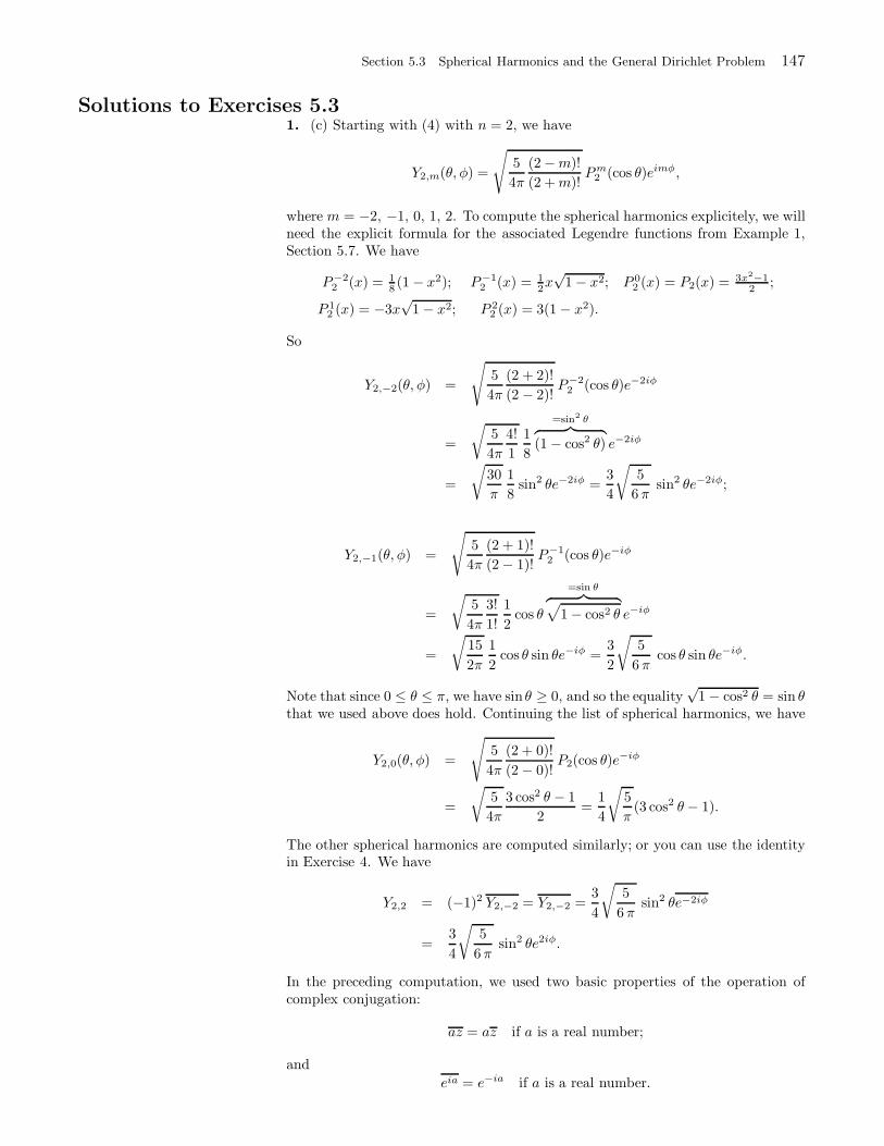
Section 5.3 Spherical Harmonics and the General Dirichlet Problem 147
Solutions to Exercises 5.31. (c) Starting with (4) with n = 2, we have
Y2,m(θ, φ) =
√5
4π
(2 −m)!
(2 +m)!Pm
2 (cos θ)eimφ,
where m = −2, −1, 0, 1, 2. To compute the spherical harmonics explicitely, we willneed the explicit formula for the associated Legendre functions from Example 1,Section 5.7. We have
P−22 (x) = 1
8(1 − x2); P−1
2 (x) = 12x√
1 − x2; P 02 (x) = P2(x) = 3x2−1
2;
P 12 (x) = −3x
√1 − x2; P 2
2 (x) = 3(1 − x2).
So
Y2,−2(θ, φ) =
√5
4π
(2 + 2)!
(2 − 2)!P−2
2 (cos θ)e−2iφ
=
√5
4π
4!
1
1
8
=sin2 θ︷ ︸︸ ︷(1 − cos2 θ) e−2iφ
=
√30
π
1
8sin2 θe−2iφ =
3
4
√5
6 πsin2 θe−2iφ;
Y2,−1(θ, φ) =
√5
4π
(2 + 1)!
(2 − 1)!P−1
2 (cos θ)e−iφ
=
√5
4π
3!
1!
1
2cos θ
=sin θ︷ ︸︸ ︷√1 − cos2 θ e−iφ
=
√15
2π
1
2cos θ sin θe−iφ =
3
2
√5
6 πcos θ sin θe−iφ.
Note that since 0 ≤ θ ≤ π, we have sin θ ≥ 0, and so the equality√
1 − cos2 θ = sin θthat we used above does hold. Continuing the list of spherical harmonics, we have
Y2,0(θ, φ) =
√5
4π
(2 + 0)!
(2 − 0)!P2(cos θ)e−iφ
=
√5
4π
3 cos2 θ − 1
2=
1
4
√5
π(3 cos2 θ− 1).
The other spherical harmonics are computed similarly; or you can use the identityin Exercise 4. We have
Y2,2 = (−1)2 Y2,−2 = Y2,−2 =3
4
√5
6 πsin2 θe−2iφ
=3
4
√5
6 πsin2 θe2iφ.
In the preceding computation, we used two basic properties of the operation ofcomplex conjugation:
az = az if a is a real number;
and
eia = e−ia if a is a real number.
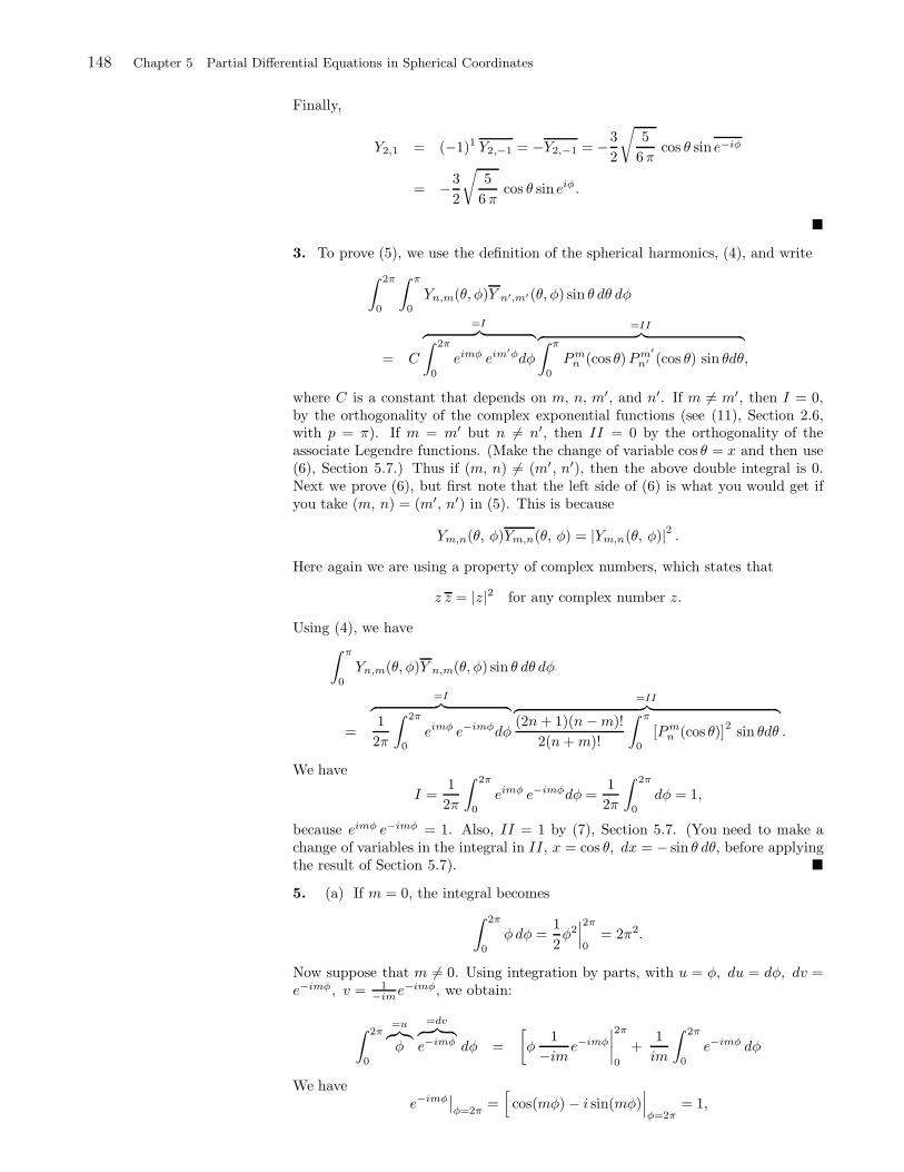
148 Chapter 5 Partial Differential Equations in Spherical Coordinates
Finally,
Y2,1 = (−1)1 Y2,−1 = −Y2,−1 = −3
2
√5
6 πcos θ sin e−iφ
= −3
2
√5
6 πcos θ sin eiφ.
3. To prove (5), we use the definition of the spherical harmonics, (4), and write
∫ 2π
0
∫ π
0
Yn,m(θ, φ)Y n′,m′ (θ, φ) sin θ dθ dφ
= C
=I︷ ︸︸ ︷∫ 2π
0
eimφ eim′φdφ
=II︷ ︸︸ ︷∫ π
0
Pmn (cos θ)Pm′
n′ (cos θ) sin θdθ,
where C is a constant that depends on m, n, m′, and n′. If m 6= m′, then I = 0,by the orthogonality of the complex exponential functions (see (11), Section 2.6,with p = π). If m = m′ but n 6= n′, then II = 0 by the orthogonality of theassociate Legendre functions. (Make the change of variable cos θ = x and then use(6), Section 5.7.) Thus if (m, n) 6= (m′, n′), then the above double integral is 0.Next we prove (6), but first note that the left side of (6) is what you would get ifyou take (m, n) = (m′, n′) in (5). This is because
Ym,n(θ, φ)Ym,n(θ, φ) = |Ym,n(θ, φ)|2 .
Here again we are using a property of complex numbers, which states that
z z = |z|2 for any complex number z.
Using (4), we have
∫ π
0
Yn,m(θ, φ)Y n,m(θ, φ) sin θ dθ dφ
=
=I︷ ︸︸ ︷1
2π
∫ 2π
0
eimφ e−imφdφ
=II︷ ︸︸ ︷(2n+ 1)(n −m)!
2(n+m)!
∫ π
0
[Pmn (cos θ)]
2sin θdθ .
We have
I =1
2π
∫ 2π
0
eimφ e−imφdφ =1
2π
∫ 2π
0
dφ = 1,
because eimφ e−imφ = 1. Also, II = 1 by (7), Section 5.7. (You need to make achange of variables in the integral in II, x = cos θ, dx = − sin θ dθ, before applyingthe result of Section 5.7).
5. (a) If m = 0, the integral becomes
∫ 2π
0
φ dφ =1
2φ2∣∣∣2π
0= 2π2.
Now suppose that m 6= 0. Using integration by parts, with u = φ, du = dφ, dv =e−imφ, v = 1
−ime−imφ, we obtain:
∫ 2π
0
=u︷︸︸︷φ
=dv︷ ︸︸ ︷e−imφ dφ =
[φ
1
−ime−imφ
∣∣∣∣2π
0
+1
im
∫ 2π
0
e−imφ dφ
We havee−imφ
∣∣φ=2π
=[cos(mφ) − i sin(mφ)
∣∣∣φ=2π
= 1,
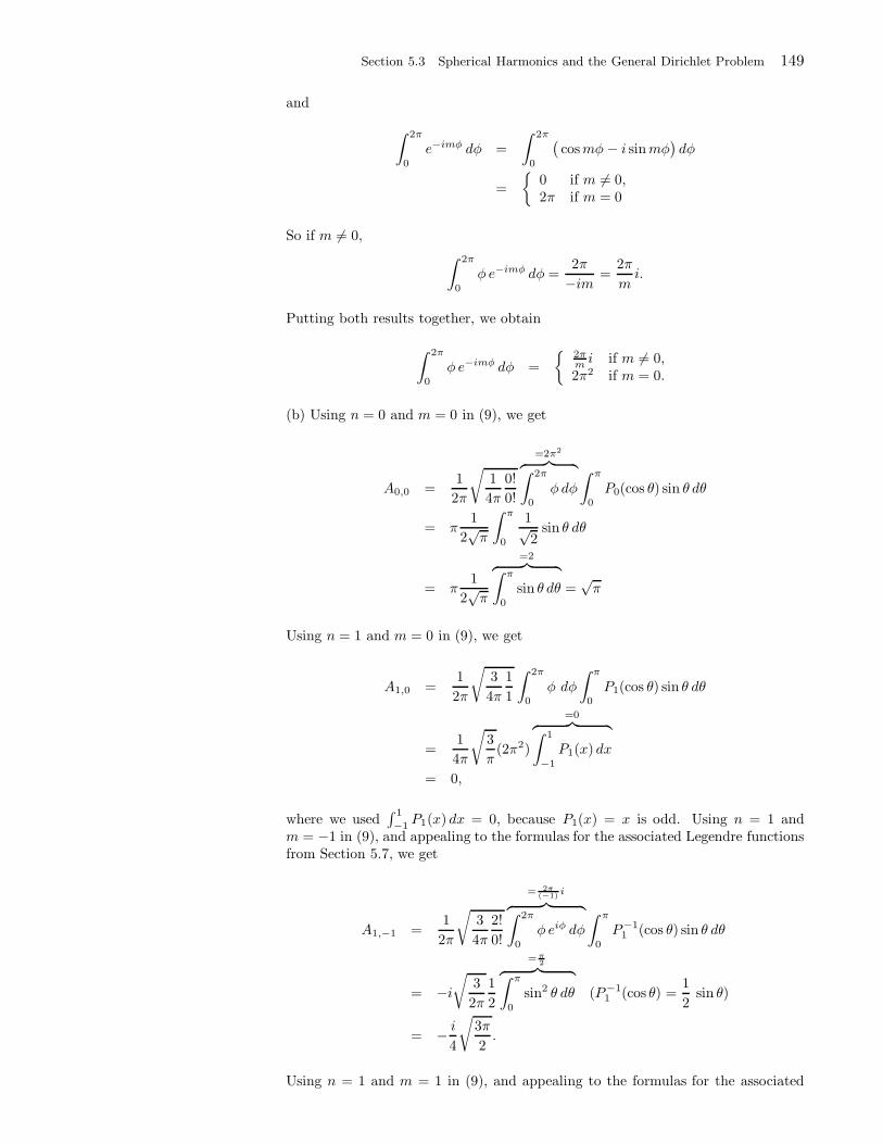
Section 5.3 Spherical Harmonics and the General Dirichlet Problem 149
and
∫ 2π
0
e−imφ dφ =
∫ 2π
0
(cosmφ − i sinmφ
)dφ
=
0 if m 6= 0,2π if m = 0
So if m 6= 0,
∫ 2π
0
φ e−imφ dφ =2π
−im =2π
mi.
Putting both results together, we obtain
∫ 2π
0
φ e−imφ dφ =
2πm i if m 6= 0,2π2 if m = 0.
(b) Using n = 0 and m = 0 in (9), we get
A0,0 =1
2π
√1
4π
0!
0!
=2π2
︷ ︸︸ ︷∫ 2π
0
φ dφ
∫ π
0
P0(cos θ) sin θ dθ
= π1
2√π
∫ π
0
1√2
sin θ dθ
= π1
2√π
=2︷ ︸︸ ︷∫ π
0
sin θ dθ =√π
Using n = 1 and m = 0 in (9), we get
A1,0 =1
2π
√3
4π
1
1
∫ 2π
0
φ dφ
∫ π
0
P1(cos θ) sin θ dθ
=1
4π
√3
π(2π2)
=0︷ ︸︸ ︷∫ 1
−1
P1(x) dx
= 0,
where we used∫ 1
−1P1(x) dx = 0, because P1(x) = x is odd. Using n = 1 and
m = −1 in (9), and appealing to the formulas for the associated Legendre functionsfrom Section 5.7, we get
A1,−1 =1
2π
√3
4π
2!
0!
= 2π(−1) i
︷ ︸︸ ︷∫ 2π
0
φ eiφ dφ
∫ π
0
P−11 (cos θ) sin θ dθ
= −i√
3
2π
1
2
=π2︷ ︸︸ ︷∫ π
0
sin2 θ dθ (P−11 (cos θ) =
1
2sin θ)
= − i
4
√3π
2.
Using n = 1 and m = 1 in (9), and appealing to the formulas for the associated
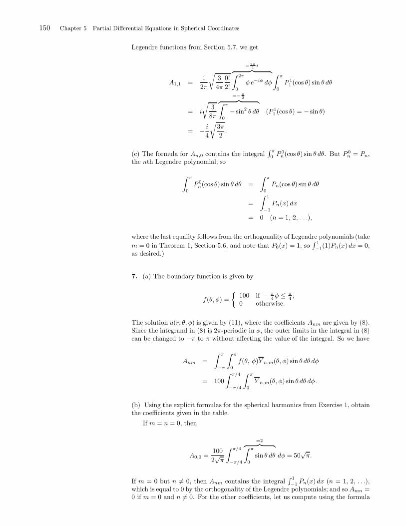
150 Chapter 5 Partial Differential Equations in Spherical Coordinates
Legendre functions from Section 5.7, we get
A1,1 =1
2π
√3
4π
0!
2!
= 2π1 i
︷ ︸︸ ︷∫ 2π
0
φ e−iφ dφ
∫ π
0
P 11 (cos θ) sin θ dθ
= i
√3
8π
=−π2︷ ︸︸ ︷∫ π
0
− sin2 θ dθ (P 11 (cos θ) = − sin θ)
= − i
4
√3π
2.
(c) The formula for An,0 contains the integral∫ π
0 P 0n(cos θ) sin θ dθ. But P 0
n = Pn,the nth Legendre polynomial; so
∫ π
0
P 0n(cos θ) sin θ dθ =
∫ π
0
Pn(cos θ) sin θ dθ
=
∫ 1
−1
Pn(x) dx
= 0 (n = 1, 2, . . .),
where the last equality follows from the orthogonality of Legendre polynomials (take
m = 0 in Theorem 1, Section 5.6, and note that P0(x) = 1, so∫ 1
−1(1)Pn(x) dx = 0,
as desired.)
7. (a) The boundary function is given by
f(θ, φ) =
100 if − π
4 φ ≤ π4 ;
0 otherwise.
The solution u(r, θ, φ) is given by (11), where the coefficients Anm are given by (8).Since the integrand in (8) is 2π-periodic in φ, the outer limits in the integral in (8)can be changed to −π to π without affecting the value of the integral. So we have
Anm =
∫ π
−π
∫ π
0
f(θ, φ)Y n,m(θ, φ) sin θ dθ dφ
= 100
∫ π/4
−π/4
∫ π
0
Y n,m(θ, φ) sin θ dθ dφ .
(b) Using the explicit formulas for the spherical harmonics from Exercise 1, obtainthe coefficients given in the table.
If m = n = 0, then
A0,0 =100
2√π
∫ π/4
−π/4
=2︷ ︸︸ ︷∫ π
0
sin θ dθ dφ = 50√π.
If m = 0 but n 6= 0, then Anm contains the integral∫ 1
−1Pn(x) dx (n = 1, 2, . . .),
which is equal to 0 by the orthogonality of the Legendre polynomials; and so Amn =0 if m = 0 and n 6= 0. For the other coefficients, let us compute using the formula
Section 5.3 Spherical Harmonics and the General Dirichlet Problem 151
for the spherical harmonics:
Anm = 100
√2n+ 1
4π
(n−m)!
(n+m)!
∫ π/4
−π/4
e−imφ dφ
∫ π
0
Pmn (cos θ) sin θ dθ
= 100
√2n+ 1
4π
(n−m)!
(n+m)!
= 2m sin mπ
4︷ ︸︸ ︷∫ π/4
−π/4
(cosmφ − i sinmφ) dφ
∫ 1
−1
Pmn (s) ds
=200
m
√2n+ 1
4π
(n−m)!
(n+m)!sin
mπ
4
∫ 1
−1
Pmn (s) ds.
The integral Inm =∫ 1
−1 Pmn (s) ds can be evaluated for particular values of m and n
(or you can use the general formula from Exercises 6). For example, if m = n = 1,then
∫ 1
−1
P 11 (s) ds = −
=half area of a disk of radius 1︷ ︸︸ ︷∫ 1
−1
√1 − s2 ds = −π
2.
So
A1,1 =200
1
√3
4π
0!
2!sin
π
4(−π
2) = −25
√3π.
The other coefficients are computed similarly by appealing to the explicit formulasfor the associated Legendre functions from Section 5.7 and using the precedingformulas.
(c) Using an approximation of the solution with n running from 0 to 2 and mrunning from −n to n, we get
u(r, θ, φ) =
∞∑
n=0
n∑
m=−n
AnmrnYn,m(θ, φ) ≈
2∑
n=0
n∑
m=−n
AnmrnYn,m(θ, φ).
Now substituting the explicit formulas and values, we obtain
u(r, θ, φ)
≈ r0Y0,0A0,0 + r1Y1,−1A1,−1 + r1Y1,1A1,1 + r2Y2,−2A2,−2 + r2Y2,2A2,2
=1
2√π
50√π + r
[1
2
√3
2πsin θ e−iφ 25
√3π +
1
2
√3
2πsin θ eiφ 25
√3π
]
+r2
[3
4
√5
6πsin2 θe−2iφ100
√5
6π+
3
4
√5
6πsin2 θe2iφ100
√5
6π
]
= 25 + 75
√2
2r sin θ
=cos φ︷ ︸︸ ︷(eiφ + e−iφ
2
)+125 r2
1
πsin2 θ
=cos 2φ︷ ︸︸ ︷(e2iφ + e−2iφ
2
)
= 25 + 75
√2
2r sin θ cos φ+ 125 r2
1
πsin2 θ cos 2φ .
9. We apply (11). Since f is its own spherical harmonics series, we have
u(r, θ, φ) = Y0,0(θ, φ) =1
2√π.
152 Chapter 5 Partial Differential Equations in Spherical Coordinates
11. The solution is very much like the solution of Exercise 7. In our case, we have
Anm = 50
√2n+ 1
4π
(n −m)!
(n +m)!
∫ π/3
−π/3
e−imφ dφ
∫ π
0
Pmn (cos θ) sin θ dθ
= 50
√2n+ 1
4π
(n −m)!
(n +m)!
= 2m sin mπ
3︷ ︸︸ ︷∫ π/3
−π/3
(cosmφ− i sinmφ) dφ
∫ 1
−1
Pmn (s) ds
=100
m
√2n+ 1
4π
(n−m)!
(n+m)!sin
mπ
3
∫ 1
−1
Pmn (s) ds
=100
m
√2n+ 1
4π
(n−m)!
(n+m)!sin
mπ
3Inm,
where Inm =∫ 1
−1Pm
n (s) ds. Several values of Inm were found previously. You canalso use the result of Exercise 6 to evaluate it.
Section 5.4 The Helmholtz, Poisson, Heat, and Wave Equations 153
Solutions to Exercises 5.4
5. We apply Theorem 3 and note that since f depends only on r and not on θor φ, the series expansion should also not depend on θ or φ. So all the coefficientsin the series are 0 except for the coefficients Aj,0,0, which we will write as Aj forsimplicity. Using (16) with m = n = 0, a = 1, f(r, θ, φ) = 1, and Y0,0(θ, φ) = 1
2√
π,
we get
Aj =2
j21(α 12 , j)
∫ 1
0
∫ 2π
0
∫ π
0
j0(λ0, j r)1
2√πr2 sin θ dθ dφ dr
=1√
π j21(α 12 , j)
=2π︷ ︸︸ ︷∫ 2π
0
dφ
=2︷ ︸︸ ︷∫ π
0
sin θ dθ
∫ 1
0
j0(λ0, j r)r2 dr
=4√π
j21(α 12 , j)
∫ 1
0
j0(λ0, j r)r2 dr,
where λ0, j = α 12 , j , the jth zero of the Bessel function of order 1
2. Now
J1/2(x) =
√2
πxsinx
(see Example 1, Section 4.7), so the zeros of J1/2 are precisely the zeros of sinx,which are jπ. Hence
λ0, j = α 12 , j = jπ.
Also, recall that
j0(x) =sinx
x
(Exercises 38, Section 4.8), so
∫ 1
0
j0(λ0, j r)r2 dr =
∫ 1
0
j0(jπ r)r2 dr =
∫ 1
0
sin(jπr)
jπ rr2 dr
=1
jπ
= (−1)j+1
jπ︷ ︸︸ ︷∫ 1
0
sin(jπ r)r dr
=(−1)j+1
(jπ)2,
where the last integral follows by integration by parts. So,
Aj =4√π
j21(jπ)
(−1)j+1
(jπ)2.
This can be simplified by using a formula for j1. Recall from Exercise 38, Sec-tion 4.7,
j1(x) =sinx− x cosx
x2.
Hence
j21(jπ) =
[sin(jπ) − jπ cos(jπ)
(jπ)2
]2=
[− cos(jπ)
jπ
]2=
[(−1)j+1
jπ
]2=
1
(jπ)2,
and
Aj = 4(−1)j+1√π,
154 Chapter 5 Partial Differential Equations in Spherical Coordinates
and so the series expansion becomes: for 0 < r < 1,
1 =
∞∑
j=1
4(−1)j+1√π
sin jπr
jπrY0,0(θ, φ)
=
∞∑
j=1
4(−1)j+1√π
sin jπr
jπr
1
2√π
=
∞∑
j=1
2(−1)j+1 sin jπr
jπr.
It is interesting to note that this series is in fact a half range sine series expansion.Indeed, multiplying both sides by r, we get
r =2
π
∞∑
j=1
(−1)j+1 sin jπr
j(0 < r < 1),
which is a familiar sines series expansion (compare with Example 1, Section 2.4).
7. Reasoning as we did in Exercise 5, we infer that the series representation is ofthe form ∞∑
j=1
AjY0,0(θ, φ)j0(α 12 , jr),
where
Aj =2
j21(α 12 , j)
∫ 1
0
∫ 2π
0
∫ π
0
j0(λ0, j r)1
2√πr4 sin θ dθ dφ dr
=1√
π j21(α 12 , j)
=2π︷ ︸︸ ︷∫ 2π
0
dφ
=2︷ ︸︸ ︷∫ π
0
sin θ dθ
∫ 1
0
j0(λ0, j r)r4 dr
=4√π
j21(α 12 , j)
∫ 1
0
j0(λ0, j r)r4 dr,
where λ0, j = α 12 , j , the jth zero of the Bessel function of order 1
2 . Again, fromExercise 5:
J1/2(x) =
√2
πxsinx,
λ0, j = α 12 , j = jπ,
and
j0(x) =sinx
x.
So∫ 1
0
j0(λ0, j r)r4 dr =
∫ 1
0
j0(jπ r)r4 dr =
∫ 1
0
sin(jπr)
jπ rr4 dr
=1
jπ
=(−6+j2π2)(−1)j+1
(jπ)3︷ ︸︸ ︷∫ 1
0
sin(jπ r)r3 dr
=(−6 + j2π2)(−1)j+1
(jπ)4,
where the last integral follows by three integrations by parts. So,
Aj =4√π
j21(jπ)
(−1)j+1(−6 + j2π2)
(jπ)4.
Section 5.4 The Helmholtz, Poisson, Heat, and Wave Equations 155
From Exercise 5,
j41(jπ) =
[sin(jπ) − jπ cos(jπ)
(jπ)2
]4=
[− cos(jπ)
jπ
]4=
[(−1)j+1
jπ
]4=
1
(jπ)4,
so
Aj = 4(−1)j+1√π
(−6 + j2π2)
(jπ)3,
and so the series expansion becomes: for 0 < r < 1,
r2 =∞∑
j=1
4(−1)j+1√π
sin jπr
(jπ)3r(−6 + j2π2)
1
2√π
=
∞∑
j=1
2(−1)j+1(−6 + j2π2)sin jπr
(jπ)3r.
Here again, it is interesting to note that this series is a half range sine series expan-sion. Indeed, multiplying both sides by r, we get
r3 =
∞∑
j=1
2(−1)j+1(−6 + j2π2)sin jπr
(jπ)3(0 < r < 1),
which is a sines series expansion of the function f(r) = r3, 0 < r < 1.
156 Chapter 5 Partial Differential Equations in Spherical Coordinates
Solutions to Exercises 5.5
1. Putting n = 0 in (9), we obtain
P0(x) =1
20
0∑
m=0
(−1)m (0 − 2m)!
m!(0 −m)!(0 − 2m)!x0−2m .
The sum contains only one term corresponding to m = 0. Thus
P0(x) = (−1)00!
0!0!0!x0 = 1,
because 0! = 1. For n = 1, formula (9) becomes
P1(x) =1
21
M∑
m=0
(−1)m (2 − 2m)!
m!(1 −m)!(1 − 2m)!x1−2m,
where M = 1−12 = 0. Thus the sum contains only one term corresponding to m = 0
and so
P1(x) =1
21(−1)0
2!
0!1!1!x1 = x.
For n = 2, we have M = 22 = 1 and (9) becomes
P2(x) =1
22
1∑
m=0
(−1)m (4 − 2m)!
m!(2 −m)!(2 − 2m)!x2−2m
=1
22
m=0︷ ︸︸ ︷(−1)0
4!
0!2!2!x2 +
1
22
m=1︷ ︸︸ ︷(−1)1
(4 − 2)!
1!1!0!x0
=1
46x2 +
1
4(−1)2 =
3
2x2 − 1
2.
For n = 3, we have M = 3−12 = 1 and (9) becomes
P3(x) =1
23
1∑
m=0
(−1)m (6 − 2m)!
m!(3 −m)!(3 − 2m)!x3−2m
=1
23(−1)0
6!
0!3!3!x3 +
1
23(−1)1
4!
1!2!1!x1
=5
2x3 − 3
2x.
For n = 4, we have M = 42
= 2 and (9) becomes
P4(x) =1
24
2∑
m=0
(−1)m (8 − 2m)!
m!(4 −m)!(4 − 2m)!x4−2m
=1
24
8!
0!4!4!x4 − 1
24
6!
1!3!2!x2 +
1
24
4!
2!2!0!x0
=1
8(35x4 − 30x2 + 3)
Section 5.5 Legendre’s Differential Equation 157
3. By the first formula in Exercise 2(b) (applied with n and n + 1), we have
P2n(0) − P2n+2(0) = = P2n(0) − P2(n+1)(0)
= (−1)n (2n)!
22n(n!)2− (−1)n+1 (2(n + 1))!
22(n+1)((n + 1)!)2
= (−1)n (2n)!
22n(n!)2+ (−1)n (2n+ 2)(2n+ 1)((2n)!)
4 22n(n + 1)2(n!)2
= (−1)n (2n)!
22n(n!)2
[1 +
(2n+ 2)(2n+ 1)
4 (n+ 1)2
]
= (−1)n (2n)!
22n(n!)2
[1 +
2(n+ 1)(2n+ 1)
4 (n+ 1)2
]
= (−1)n (2n)!
22n(n!)2
[1 +
(2n+ 1)
2 (n+ 1)
]
= (−1)n (2n)!(4n+ 3)
22n+1(n!)2(n+ 1)
5. Using the explicit formulas for the Legendre polynomials, we find
∫ 1
−1
P3(x) dx =
∫ 1
−1
(5
2x3 − 3
2x) dx
= (5
8x4 − 3
4x2)
∣∣∣∣1
−1
= 0
Another faster way to see the answer is to simply note that P3 is an odd function, soits integral over any symmetric interval is 0. There is yet another more importantreason for this integral to equal 0. In fact,
∫ 1
−1
Pn(x) dx = 0 for all n 6= 0.
This is a consequence of orthogonality that you will study in Section 5.6.
7. Using the explicit formulas for the Legendre polynomials, we find
∫ 1
0
P2(x) dx =
∫ 1
0
(3
2x2 − 1
2) dx
= (1
2x3 − 1
2x)
∣∣∣∣1
0
= 0
This integral is a special case of a more general formula presented in Exercise 10,Section 5.6.
9. This is Legendre’s equation with n(n + 1) = 30 so n = 5. Its general solutionis of the form
y = c1P5(x) + c2Q5(x)
= c11
8(63x5 − 70x3 + 15x) + c2
(1 − 15x2 + 30x4 + · · ·
)
= c1(63x5 − 70x3 + 15x) + c2(1 − 15x2 + 30x4 + · · ·
)
In finding P5(x), we used the given formulas in the text. In finding the first fewterms of Q5(x), we used (3) with n = 5. (If you are comparing with the answers inyour textbook, just remember that c1 and c2 are arbitrary constants.)
11. This is Legendre’s equation with n(n + 1) = 0 so n = 0. Its general solution
158 Chapter 5 Partial Differential Equations in Spherical Coordinates
is of the form
y = c1P0(x) + c2Q0(x)
= c1 + c2
(x− −2
6x3 +
24
5!x5 + · · ·
)
= c1 + c2
(x+
x3
3+x5
5+ · · ·
)
where we used P0(x) = 1 and (4) with n = 0.
13. This is Legendre’s equation with n(n + 1) = 6 or n = 2. Its general solutionis y = c1P2(x) + c2Q2(x). The solution will be bounded on [−1, 1] if and onlyif c2 = 0; that’s because P2 is bounded in [−1, 1] but Q2 is not. Now, usingP2(x) = 1
2(3x2 − 1), we find
y(0) = c1P2(0) + c2Q2(0) = −c12
+ c2Q2(0)
If c2 = 0, then c1 = 0 and we obtain the zero solution, which is not possible (sincewe are given y′(0) = 1, the solution is not identically 0). Hence c2 6= 0 and thesolutions is not bounded.
15. This is Legendre’s equation with n(n+ 1) = 56 or n = 7. Its general solutionis y = c1P7(x) + c2Q2(x). The solution will be bounded on [−1, 1] if and only ifc2 = 0. Since P7(x) is odd, we have P7(0) = 0 and so
1 = y(0) = c1P7(0) + c2Q7(0) = c2Q2(0).
This shows that c2 6= 0 and the solutions is not bounded.
17. (To do this problem we can use the recurrence relation for the coefficients,as we have done below in the solution of Exercise 19. Instead, we offer a differentsolution based on an interesting observation.) This is Legendre’s equation withn(n+1) = 3
4or n = 1
2. Its general solution is still given by (3) and (4), with n = 1
2:
y = c1y1 + c2y2,
where
y1(x) = 1 −12(12
+ 1)
2!x2 +
(12− 2)1
2(12
+ 1)(12
+ 3)
4!x4 + · · ·
= 1 − 3
8x2 − 21
128x4 + · · ·
and
y2(x) = x− (12− 1)(1
2+ 2)
3!x3 +
(12− 3)(1
2− 1)(1
2+ 2)(1
2+ 4)
5!x5 + · · ·
= x+5
24x3 +
15
128x5 + · · ·
Since y1(0) = 1 and y2(0) = 0, y′1(0) = 0 and y′2(0) = 1 (differentiate the series termby term, then evaluate at x = 0), it follows that the solution is y = y1(x) + y2(x),where y1 and y2 are as describe above.
19. This is Legendre’s equation with µ = 3. Its solutions have series expansionsy =
∑∞m=0 amx
m for −1 < x < 1, where
am+2 =m(m + 1) − µ
(m+ 2)(m+ 1)am .
Since y(0) = 0 and y′(0) = 1, we find that a0 = 0 and a1 = 1. Now because therecurrence relation is a two-step recurrence, we obtain
0 = a0 = a2 = a4 = · · ·
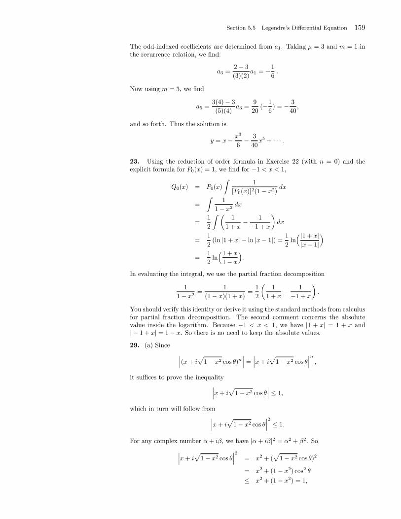
Section 5.5 Legendre’s Differential Equation 159
The odd-indexed coefficients are determined from a1. Taking µ = 3 and m = 1 inthe recurrence relation, we find:
a3 =2 − 3
(3)(2)a1 = −1
6.
Now using m = 3, we find
a5 =3(4) − 3
(5)(4)a3 =
9
20(−1
6) = − 3
40,
and so forth. Thus the solution is
y = x− x3
6− 3
40x5 + · · · .
23. Using the reduction of order formula in Exercise 22 (with n = 0) and theexplicit formula for P0(x) = 1, we find for −1 < x < 1,
Q0(x) = P0(x)
∫1
[P0(x)]2(1 − x2)dx
=
∫1
1 − x2dx
=1
2
∫ (1
1 + x− 1
−1 + x
)dx
=1
2(ln |1 + x| − ln |x− 1|) =
1
2ln( |1 + x||x− 1|
)
=1
2ln(1 + x
1 − x
).
In evaluating the integral, we use the partial fraction decomposition
1
1 − x2=
1
(1 − x)(1 + x)=
1
2
(1
1 + x− 1
−1 + x
).
You should verify this identity or derive it using the standard methods from calculusfor partial fraction decomposition. The second comment concerns the absolutevalue inside the logarithm. Because −1 < x < 1, we have |1 + x| = 1 + x and| − 1 + x| = 1 − x. So there is no need to keep the absolute values.
29. (a) Since
∣∣∣(x+ i√
1 − x2 cos θ)n∣∣∣ =
∣∣∣x+ i√
1 − x2 cos θ∣∣∣n
,
it suffices to prove the inequality
∣∣∣x+ i√
1 − x2 cos θ∣∣∣ ≤ 1,
which in turn will follow from
∣∣∣x+ i√
1 − x2 cos θ∣∣∣2
≤ 1.
For any complex number α+ iβ, we have |α+ iβ|2 = α2 + β2. So
∣∣∣x+ i√
1 − x2 cos θ∣∣∣2
= x2 + (√
1 − x2 cos θ)2
= x2 + (1 − x2) cos2 θ
≤ x2 + (1 − x2) = 1,

160 Chapter 5 Partial Differential Equations in Spherical Coordinates
which proves the desired inequality.(b) Using Laplace’s formula, we have, for −1 ≤ x ≤ 1,
|Pn(x)| =1
π
∣∣∣∣∫ π
0
(x + i√
1 − x2 cos θ)n dθ
∣∣∣∣
≤ 1
π
∫ π
0
∣∣∣(x+ i√
1 − x2 cos θ)n∣∣∣ dθ
≤ 1
π
∫ π
0
dθ (by (a))
= 1
31. Recall that if α is any real number and k is a nonnegative integer, the kthbinomial coefficient is
(αk
)=α(α− 1)(α− 2) . . . (α− k + 1)
k!for k ≥ 1
and
(α0
)= 1. With this notation, the binomial theorem asserts that
(1 + x)α =
∞∑
k=0
(αk
)xk, −1 < x < 1 .
(a) Set α = −12 , and obtain that
1√1 + v
=∞∑
k=0
(−1)k (2k)!
22k(k!)2vk, |v| < 1 .
Solution We have
(−1/2k
)=
1
k!
k factors︷ ︸︸ ︷−1
2
(−1
2− 1
)· · ·(−1
2− (k − 1)
)
=1
k!
−1
2
(−3
2
)· · ·(−(2k − 1)
2
)
=1
k!
(−1)k
2k[1 · 3 · · · (2k − 1)]
=1
k!
(−1)k
2k
[1 · 2 · 3 · 4 · · · (2k − 1) · (2k)]2 · 4 · · · (2k)
=1
k!
(−1)k
2k
(2k)!
(2 · 1) · (2 · 2) · · · (2 · k)
=1
k!
(−1)k
2k
(2k)!
2k(k!)=
(−1)k(2k)!
22k(k!)2
So, for |v| < 1, the binomial series gives
1√1 + v
= (1 + v)−1/2 =
∞∑
k=0
(−1/2k
)vk =
∞∑
k=0
(−1)k (2k)!
22k(k!)2vk
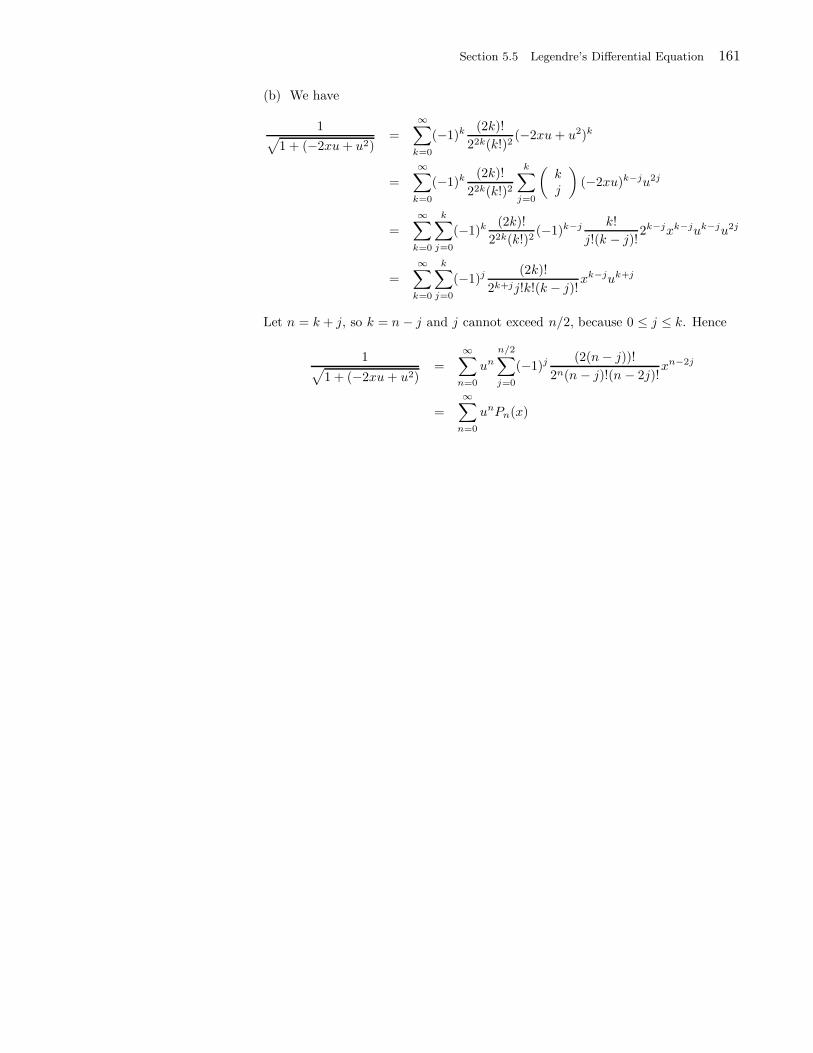
Section 5.5 Legendre’s Differential Equation 161
(b) We have
1√1 + (−2xu+ u2)
=
∞∑
k=0
(−1)k (2k)!
22k(k!)2(−2xu+ u2)k
=
∞∑
k=0
(−1)k (2k)!
22k(k!)2
k∑
j=0
(kj
)(−2xu)k−ju2j
=
∞∑
k=0
k∑
j=0
(−1)k (2k)!
22k(k!)2(−1)k−j k!
j!(k − j)!2k−jxk−juk−ju2j
=
∞∑
k=0
k∑
j=0
(−1)j (2k)!
2k+jj!k!(k − j)!xk−juk+j
Let n = k + j, so k = n − j and j cannot exceed n/2, because 0 ≤ j ≤ k. Hence
1√1 + (−2xu+ u2)
=
∞∑
n=0
un
n/2∑
j=0
(−1)j (2(n− j))!
2n(n − j)!(n − 2j)!xn−2j
=
∞∑
n=0
unPn(x)
162 Chapter 5 Partial Differential Equations in Spherical Coordinates
Solutions to Exercises 5.6
1. Bonnet’s relation says: For n = 1, 2, . . . ,
(n+ 1)Pn+1(x) + nPn−1(x) = (2n+ 1)xPn(x).
We have P0(x) = 1 and P1(x) = x. Take n = 1, then
2P2(x) + P0(x) = 3xP1(x),
2P2(x) = 3x · x− 1,
P2(x) =1
2(3x2 − 1).
Take n = 2 in Bonnet’s relation, then
3P3(x) + 2P1(x) = 5xP2(x),
3P3(x) = 5x(12(3x2 − 1)
)− 2x,
P3(x) =5
2x3 − 3
2x.
Take n = 3 in Bonnet’s relation, then
4P4(x) + 3P2(x) = 7xP3(x),
4P4(x) = 7x(52x3 − 3
2x)− 3
2
(x2 − 1
),
P4(x) =1
4
[35
2x4 − 15x2 +
3
2
].
3. ∫ 1
−1
xP7(x) dx =
∫ 1
−1
P1(x)P7(x) dx = 0,
by Theorem 1(i).
5. By Bonnet’s relation with n = 3,
7xP3(x) = 4P4(x) + 3P2(x),
xP3(x) =4
7P4(x) +
3
7P2(x).
So
∫ 1
−1
xP2(x)P3(x) dx =
∫ 1
−1
(4
7P4(x) +
3
7P2(x)
)P2(x) dx
=4
7
∫ 1
−1
P4(x)P2(x) dx+3
7
∫ 1
−1
[P2(x)]2 dx
= 0 +3
7
2
5=
6
35,
where we have used Theorem 1(i) and (ii) to evaluate the last two integrals.
7.
∫ 1
−1
x2 P7(x) dx = 0, because x2 is even and P7(x) is odd. So their product is
odd, and the integral of any odd function over a symmetric interval is 0.
Section 5.6 Legendre Polynomials and Legendre Series Expansions 163
9. (a) Write (4) in the form
(2n+ 1)Pn(t) = P ′n+1(t) − P ′
n−1(t).
Integrate from x to 1,
(2n+ 1)
∫ 1
x
Pn(t) dt =
∫ 1
x
P ′n+1(t) dt−
∫ 1
x
P ′n−1(t) dt
= Pn+1(t)∣∣∣1
x− Pn−1(t)
∣∣∣1
x
=(Pn−1(x) − Pn+1(x)
)+(Pn+1(1) − Pn−1(1)
).
By Example 1, we have Pn+1(1) − Pn−1(1) = 0. So for n = 1, 2, . . .
∫ 1
x
Pn(t) dt =1
2n+ 1[Pn−1(x) − Pn+1(x)] .
(b) First let us note that because Pn is even when is even and odd when is odd, itfollows that Pn(−1) = (−1)nPn(1) = (−1)n. Taking x = −1 in (a), we get
∫ 1
−1
Pn(t) dt =1
2n+ 1[Pn−1(−1) − Pn+1(−1)] = 0,
because n−1 and n+1 are either both even or both odd, so Pn−1(−1) = Pn+1(−1).(c) We have
0 =
∫ 1
−1
Pn(t) dt =
∫ x
−1
Pn(t) dt+
∫ 1
x
Pn(t) dt.
So
∫ x
−1
Pn(t) dt = −∫ 1
x
Pn(t) dt
= − 1
2n+ 1[Pn−1(x) − Pn+1(x)]
=1
2n+ 1[Pn+1(x) − Pn−1(x)]
11. (a)
∫ 1
0
xP0(x) dx =
∫ 1
0
x dx =1
2;
∫ 1
0
xP1(x) dx =
∫ 1
0
x2 dx =1
3
(b) Using Bonnet’s relation (with 2n in place of n):
xP2n =1
4n+ 1[(2n+ 1)P2n+1(x) + 2nP2n−1(x)] .
164 Chapter 5 Partial Differential Equations in Spherical Coordinates
So, using Exercise 10 (with n and n− 1), we find
∫ 1
0
xP2n(x) dx =1
4n+ 1
[(2n+ 1)
∫ 1
0
P2n+1(x) dx+ 2n
∫ 1
0
P2n−1(x) dx
]
=1
4n+ 1
[(2n+ 1)
(−1)n(2n)!
22n+1(n!)2(n+ 1)+ 2n
(−1)n−1(2(n− 1))!
22(n−1)+1((n − 1)!)2n
]
=(−1)n
4n+ 1
(2n− 2)!
22n(n!)2(n + 1)
[(2n+ 1)
(2n)(2n− 1)
2− 4(n + 1)n2
]
=(−1)n
4n+ 1
(2n− 2)!
22n(n!)2(n + 1)[−n(4n+ 1)]
=(−1)n+1(2n− 2)!
22n((n− 1)!)2n(n+ 1)
Using Bonnet’s relation (with 2n+ 1 in place of n):
xP2n+1 =1
4n+ 3[(2n+ 2)P2n+2(x) + (2n+ 1)P2n(x)] .
Now using Exercise 10, it follows that∫ 1
0 xP2n+1(x) dx = 0.
13. We will use Dnf to denote the nth derivative of f . Using Exercise 12,
∫ 1
−1
(1 − x2)P13(x) dx =(−1)13
213(13)!
∫ 1
−1
D13[(1 − x2)] (x2 − 1)13 dx = 0
because D13[(1 − x2)] = 0.
15. Using Exercise 12,
∫ 1
−1
xn Pn(x) dx =(−1)n
2nn!
∫ 1
−1
Dn[xn] (x2 − 1)n dx
=(−1)n
2n
∫ 1
−1
(x2 − 1)n dx
=(−1)n
2n
∫ π
0
(cos2 θ− 1)n sin θdθ =1
2n
∫ π
0
sin2n+1 θdθ
(Let x = cos θ, dx = − sin θdθ.)
=1
2n
∫ π/2
0
sin2n+1 θdθ +1
2n
∫ π
π/2
sin2n+1 θdθ
=1
2n
∫ π/2
0
sin2n+1 θdθ +1
2n
∫ π/2
0
sin2n+1(θ +π
2)dθ
=1
2n
∫ π/2
0
sin2n+1 θdθ +1
2n
∫ π/2
0
cos2n+1 θdθ (sin(θ +π
2) = cos θ)
=2
2n
∫ π/2
0
sin2n+1 θdθ =2
2n
22n(n!)2
(2n+ 1)!=
2n+1(n!)2
(2n+ 1)!,
where we have used the results of Exercises 41 and 42, Section 4.7.
Section 5.6 Legendre Polynomials and Legendre Series Expansions 165
17. Using Exercise 12,∫ 1
−1
ln(1 − x)P2(x) dx =(−1)2
222!
∫ 1
−1
D2 [ln(1 − x)] (x2 − 1)2 dx
=1
8
∫ 1
−1
−1
(1 − x)2(x− 1)2(x+ 1)2 dx
=−1
8
∫ 1
−1
(x+ 1)2 dx =−1
24(x+ 1)3
∣∣∣1
−1=
−1
3.
21. For n > 0, we have
Dn[ln(1 − x)] =−(n − 1)!
(1 − x)n.
So∫ 1
−1
ln(1 − x)Pn(x) dx =(−1)n
2nn!
∫ 1
−1
Dn[ln(1 − x)] (x2 − 1)n dx
=(−1)n+1(n− 1)!
2nn!
∫ 1
−1
(x+ 1)n(x− 1)n
(1 − x)ndx
=−1
2nn
∫ 1
−1
(x+ 1)n dx =−1
2nn(n+ 1)(x+ 1)n+1
∣∣∣1
−1
=−2
n(n+ 1)
For n = 0, we use integration by parts. The integral is a convergent improperintegral (the integrand has a problem at 1)
∫ 1
−1
ln(1 − x)P0(x) dx =
∫ 1
−1
ln(1 − x) dx
= −(1 − x) ln(1 − x) − x∣∣∣1
−1= −2 + 2 ln2.
To evaluate the integral at x = 1, we used limx→1(1 − x) ln(1 − x) = 0.
27. Let f(x) = |x|, −1 ≤ x ≤ 1. (a) We have
A0 =1
2
∫ 1
−1
|x|P0(x) dx
=
∫ 1
0
x dx =1
2
A1 =2 + 1
2
∫ 1
−1
|x| x dx= 0
(Because the integrand is odd.)
A2 =5
2
∫ 1
−1
|x| 12(3x2 − 1) dx
=5
2
∫ 1
0
x (3x2 − 1) dx =5
4.
(b) In general A2k+1 = 0, because f is even, and
A2n =4n+ 1
2
∫ 1
−1
|x|P2n(x) dx
= (4n+ 1)
∫ 1
0
xP2n(x) dx
= (4n+ 1)(−1)n+1(2n− 2)!
22n((n− 1)!)2n(n+ 1).
166 Chapter 5 Partial Differential Equations in Spherical Coordinates
by Exercise 1129. Call the function in Exercise 28 g(x). Then
g(x) =1
2(|x|+ x) =
1
2(|x|+ P1(x)) .
Let Bk denote the Legendre coefficient of g and Ak denote the Legendre coefficientof f(x) = |x|, for −1 < x < 1. Then, because P1(x) is its own Legendre series, wehave
Bk =
12Ak if k 6= 1
12 (Ak + 1) if k = 1
Using Exercise 27 to compute Ak, we find
B0 =1
2A0 =
1
4, B1 =
1
2+
1
2A1 =
1
2+ 0 =
1
2, B2n+1 = 0, n = 1, 2, . . . ,
and
B2n =1
2A2n =
(−1)n+1(2n− 2)!
22n+1((n − 1)!)2n
(4n+ 1
n+ 1
).
31. (a) For −1 < x < 1, we use the result of Exercise 30 and get and the Legendreseries
ln(1 + x) = ln(1 − (−x))
= ln 2 − 1 −∞∑
n=1
2n+ 1
n(n+ 1)Pn(−x)
= ln 2 − 1 −∞∑
n=1
(−1)n 2n+ 1
n(n+ 1)Pn(x),
because Pn(−x) = (−1)nPn(x).
Section 6.1 Orthogonal Functions 167
Solutions to Exercises 6.1
1. Let fj(x) = cos(jπx), j = 0, 1, 2, 3, and gj(x) = sin(jπx), j = 1, 2, 3. We
have to show that∫ 2
0fj(x)gk(x) dx = 0 for all possible choices of j and k. If j = 0,
then ∫ 2
0
fj(x)gk(x) dx =
∫ 2
0
sinkπx dx =−1
kπcos(kπx)
∣∣∣2
0= 0.
If j 6= 0, and j = k, then using the identity sinα cosα = 12 sin 2α,
∫ 2
0
fj(x)gj(x) dx =
∫ 2
0
cos(jπx) sin(jπx) dx
=1
2
∫ 2
0
sin(2jπx) dx
=−1
4jπcos(2jπx)
∣∣∣2
0= 0.
If j 6= 0, and j 6= k, then using the identity
sinα cosβ =1
2
(sin(α+ β) + sin(α− β)
),
we obtain
∫ 2
0
fj(x)gk(x) dx =
∫ 2
0
sin(kπx) cos(jπx) dx
=1
2
∫ 2
0
(sin(k + j)πx + sin(k − j)πx
)dx
=−1
2π
( 1
k + jcos(k + j)πx +
1
k − jcos(k − j)πx
)∣∣∣2
0= 0.
5. Let f(x) = 1, g(x) = 2x, and h(x) = −1 + 4x. We have to show that
∫ 1
−1
f(x)g(x)w(x) dx = 0,
∫ 1
−1
f(x)h(x)w(x) dx = 0,
∫ 1
−1
g(x)h(x)w(x) dx = 0.
Let’s compute:
∫ 1
−1
f(x)g(x)w(x) dx =
∫ 1
−1
2x√
1 − x2 dx = 0,
because we are integrating an odd function over a symmetric interval. For thesecond integral, we have
∫ 1
−1
f(x)h(x)w(x) dx =
∫ 1
−1
(−1 + 4x2)√
1 − x2 dx
=
∫ π
0
(−1 + 4 cos2 θ) sin2 θ dθ
(x = cos θ, dx = − sin θ dθ, sin θ ≥ 0 for 0 ≤ θ ≤ π.)
= −∫ π
0
sin2 θ dθ+ 4
∫ π
0
(cos θ sin θ)2 dθ
= −
=π2︷ ︸︸ ︷∫ π
0
1 − cos 2θ
2dθ+4
∫ π
0
(12
sin(2θ))2dθ
= −π2
+
= π2︷ ︸︸ ︷∫ π
0
1 − cos(4θ)
2dθ = 0
168 Chapter 6 Sturm-Liouville Theory with Engineering Applications
For the third integral, we have
∫ 1
−1
g(x)h(x)w(x) dx =
∫ 1
−1
2x(−1 + 4x2)√
1 − x2 dx = 0,
because we are integrating an odd function over a symmetric interval.
9. In order for the functions 1 and a+ bx+ x2 to be orthogonal, we must have
∫ 1
−1
1 · (a+ bx+ x2) dx = 0
Evaluating the integral, we find
ax+b
2x2 +
1
3x3∣∣∣1
−1= 2a+
2
3= 0
a = −1
3.
In order for the functions x and 13 + bx+ x2 to be orthogonal, we must have
∫ 1
−1
1 · (1
3+ bx+ x2)x dx = 0
Evaluating the integral, we find
1
6x2 +
b
3x3 +
1
4x4∣∣∣1
−1=
b
3= 0
b = 0.
13. Using Theorem 1, Section 5.6, we find the norm of Pn(x) to be
‖Pn‖ =
(∫ 1
−1
Pn(x)2 dx
) 12
=
(2
2n+ 1
) 12
=
√2√
2n+ 1.
Thus the orthonormal set of functions obtained from the Legendre polynomials is
√2√
2n+ 1Pn(x), n = 0, 2, . . . .
17. For Legendre series expansions, the inner product is defined in terms ofintegration against the Legendre polynomials. That is,
(f, Pj) =
∫ 1
−1
f(x)Pj(x) dx =2
2j + 1Aj
where Aj is the Legendre coefficient of f (see (7), Section 5.6). According to thegeneralized Parseval’s identity, we have
∫ 1
−1
f2(x) dx =
∞∑
j=0
|(f, Pj)|2‖Pj‖2
=
∞∑
j=0
(2
2j + 1Aj
)22
2j + 1
=
∞∑
j=0
2
2j + 1A2
j .
(The norm ‖Pj‖ is computed in Exercise 13.)
Section 6.2 Sturm-Liouville Theory 169
Solutions to Exercises 6.2
1. Sturm-Liouville form:(xy′)′
+ λy = 0, p(x) = x, q(x) = 0, r(x) = 1. Singularproblem because p(x) = 0 at x = 0.
5. Divide the equation through by x2 and get y′′
x − y′
x2 + λyx = 0. Sturm-Liouville
form:(
1xy′)′
+ λyx
= 0, p(x) = 1x, q(x) = 0, r(x) = 1
x. Singular problem because
p(x) and r(x) are not continuous at x = 0.
9. Sturm-Liouville form:((1−x2) y′
)′+λy = 0, p(x) = 1−x2, q(x) = 0, r(x) = 1.
Singular problem because p(±1) = 0.
13. Before we proceed with the solution, we can use our knowledge of Fourierseries to guess a family of orthogonal functions that satisfy the Sturm-Liouvilleproblem: yk(x) = sin 2k+1
2x, k = 0, 1, 2, . . .. It is straightforward to check the
validity of our guess. Let us instead proceed to derive these solutions. We organizeour solution after Example 2. The differential equation fits the form of (1) withp(x) = 1, q(x) = 0, and r(x) = 1. In the boundary conditions, a = 0 and b = π,with c1 = d2 = 1 and c2 = d1 = 0, so this is a regular Sturm-Liouville problem.
We consider three cases.
CASE 1: λ < 0. Let us write λ = −α2, where α > 0. Then the equation becomesy′′ − α2y = 0, and its general solution is y = c1 sinhαx + c2 coshαx. We needy(0) = 0, so substituting into the general solution gives c2 = 0. Now using thecondition y′(π) = 0, we get 0 = c1α coshαπ, and since cosh x 6= 0 for all x, we inferthat c1 = 0. Thus there are no nonzero solutions in this case.CASE 2: λ = 0. Here the general solution of the differential equation is y =c1x+ c2, and as in Case 1 the boundary conditions force c1 and c2 to be 0. Thusagain there is no nonzero solution.
CASE 3: λ > 0. In this case we can write λ = α2 with α > 0, and so theequation becomes y′′ + α2y = 0. The general solution is y = c1 cosαx+ c2 sinαx.From y(0) = 0 we get 0 = c1 cos 0 + c2 sin 0 or 0 = c1. Thus y = c2 sinαx. Nowwe substitute the other boundary condition to get 0 = c2α cosαπ. Since we areseeking nonzero solutions, we take c2 6= 0. Thus we must have cosαπ = 0, andhence α = 2k+1
2 . Since λ = α2, the problem has eigenvalues
λk =
(2k + 1
2
)2
,
and corresponding eigenfunctions
yk = sin2k + 1
2x, k = 0, 1, 2, . . . .
17. Case I If λ = 0, the general solution of the differential equation is X = ax+b.As in Exercise 13, check that the only way to satisfy the boundary conditions is totake a = b = 0. Thus λ = 0 is not an eigenvalue since no nontrivial solutions exist.
Case II If λ = −α2 < 0, then the general solution of the differential equationis X = c1 coshαx+ c2 sinhαx. We have X′ = c1α sinhx+ c2α coshαx. In order tohave nonzero solutions, we suppose throughout the solution that c1 or c2 is nonzero.The first boundary condition implies
c1 + αc2 = 0 c1 = −αc2.Hence both c1 and c2 are nonzero. The second boundary condition implies that
c1(coshα+ α sinhα) + c2(sinhα+ α coshα) = 0.
Using c1 = −αc2, we obtain
−αc2(coshα+ α sinhα) + c2(sinhα+ α coshα) = 0 (divide byc2 6= 0)
sinhα(1− α2) = 0
sinhα = 0 or 1 − α2 = 0
170 Chapter 6 Sturm-Liouville Theory with Engineering Applications
Since α 6= 0, it follows that sinhα 6= 0 and this implies that 1− α2 = 0 or α = ±1.We take α = 1, because the value −1 does not yield any new eigenfunctions. Forα = 1, the corresponding solution is
X = c1 coshx+ c2 sinhx = −c2 cosh x+ c2 sinhx,
because c1 = −αc2 = −c2. So in this case we have one negative eigenvalue λ =−α2 = −1 with corresponding eigenfunction X = cosh x− sinhx.
Case III If λ = α2 > 0, then the general solution of the differential equation is
X = c1 cosαx+ c2 sinαx .
We have X′ = −c1α sinαx+ c2α cosαx. In order to have nonzero solutions, one ofthe coefficients c1 or c2 must be 6= 0. Using the boundary conditions, we obtain
c1 + αc2 = 0
c1(cosα− α sinα) + c2(sinα+ α cosα) = 0
The first equation implies that c1 = −αc2 and so both c1 and c2 are neq0. Fromthe second equation, we obtain
−αc2(cosα− α sinα) + c2(sinα+ α cosα) = 0
−α(cosα− α sinα) + (sinα+ α cosα) = 0
sinα(α2 + 1) = 0
Since α2 + 1 6= 0, then sinα = 0, and so α = nπ, where n = 1, 2, . . .. Thus theeigenvalues are
λn = (nπ)2
with corresponding eigenfunctions
yn = −nπ cos nπx+ sinnπx, n = 1, 2, . . . .
21. If λ = α2, then the solutions are of the form c1 coshαx + c2 sinhαx. Usingthe boundary conditions, we find
y(0) = 0 ⇒ c1 = 0
y(1) = 0 ⇒ c2 sinhα = 0.
But α 6= 0, hence sinhα 6= 0, and so c2 = 0. There are no nonzero solutions if λ > 0and so the problem as no positive eigenvalues. This does not contradict Theorem 1because if we consider the equation y′′ − λy = 0 as being in the form (1), thenr(x) = −1 < 0 and so the problem is a singular Sturm-Liouville problem to whichTheorem 1 does not apply.
25. The eigenfunctions in Example 2 are yj(x) = sin jx, j = 1, 2, . . .. Since f isone of these eigenfunctions, it is equal to its own eigenfunction expansion.
29. You can verify the orthogonality directly by checking that
∫ 2π
0
sinnx
2sin
mx
2dx = 0 if m 6= n (m, n integers).
You can also quote Theorem 2(a) because the problem is a regular Sturm-Liouvilleproblem.
33. (a) From Exercise 36(b), Section 4.8, with y = J0(λr) and p = 0, we have
2λ2
∫ a
0
[y(r)]2r dr = [ay′(a)]2 + λ2a2[y(a)]2.
Section 6.2 Sturm-Liouville Theory 171
But y satisfies the boundary condition y′(a) = −κy(a), so
2λ2
∫ a
0
[y(r)]2r dr = a2κ2[y(a)]2 + λ2a2[y(a)]2;
∫ a
0
[y(r)]2r dr =a2
2
[κ2 [J0(λka)]
2
λ2k
+ [J0(λka)]2
]
=a2
2
[[J0(λka)]
2 + [J1(λka)]2],
because, by (7), [J0(λka)]2 =
[λk
κ J1(λka)]2
.(b) Reproduce the sketch of proof of Theorem 1. The given formula for the coeffi-cients is precisely formula (5) in this case.
35. Because the initial and boundary values do not depend on θ, it follows that theproblem has a radially symmetric solution that does not depend on θ. Followingthe steps in the solution of Exercise 10, Section 4.2, we find that
u(r, t) =
∞∑
k=1
Ake−λ2
ktJ0(λkr) (t > 0, 0 < r < 1),
where, due to the Robin boundary condition, the radial part R in the product so-lutions must satisfy the boundary condition R′(1) = −R(1). (If you separate vari-ables, you will arrive at the equation inR that is treated in Example 6.) Consideringthat R(r) = J0(λr), this condition gives λJ ′
0(λ) = −J0(λ). Using J ′0(r) = −J1(r),
we see that λ is a solution of equation (7): λJ1(λ) = J0(λ). Setting t = 0 and usingu(r, 0) = 100, we find that
100 =
∞∑
k=1
AkJ0(λkr),
which is the series expansion in Exercise 34. Thus
u(r, t) = 200
∞∑
k=1
J0(λk)
λ2k
([J0(λk)]2 + [J1(λk)]2
)e−λ2ktJ0(λkr) (t > 0, 0 < r < 1).
172 Chapter 6 Sturm-Liouville Theory with Engineering Applications
Solutions to Exercises 6.3
1. (a) The initial shape of the chain is given by the function
f(x) = −.01(x− .5), 0 < x < .5,
and the initial velocity of the chain is zero. So the solution is given by (10), withL = .5 and Bj = 0 for all j. Thus
u(x, t) =
∞∑
j=1
AjJ0
(αj
√2x)
cos(√
2gαj
2t).
To compute Aj , we use (11), and get
Aj =2
J21 (αj)
∫ .5
0
(−.01)(x− .5)J0
(αj
√2x)dx
=−.02
J21 (αj)
∫ .5
0
(x− .5)J0
(αj
√2x)dx
Make the change of variables s = αj
√2x, or s2 = 2α2
jx, so 2s ds = 2α2j dx or
dx = sα2
jds. Thus
Aj =−.02
J21 (αj)
∫ αj
0
(.5
α2j
s2 − .5)J0(s)s
α2j
ds
=−.01
α4jJ
21 (αj)
∫ αj
0
(s2 − α2j)J0(s)s ds
=.01
α4jJ
21 (αj)
[2α4
j
α2j
J2(αj)
]
=.02
α2jJ
21 (αj)
J2(αj),
where we have used the integral formula (15), Section 4.3, with a = α = αj. Wecan give our answer in terms of J1 by using formula (6), Section 4.8, with p = 1,and x = αj. Since αj is a zero of J0, we obtain
2
αjJ1(αj) = J0(αj) + J2(αj) = J2(αj).
So
Aj =.02
α2jJ
21 (αj)
2
αjJ1(αj) =
.04
α3jJ1(αj)
.
Thus the solution is
u(x, t) =
∞∑
j=1
.04
α3jJ1(αj)
J0
(αj
√2x)
cos(√
2gαj
2t),
where g ≈ 9.8 m/sec2.Going back to the questions, to answer (a), we have the normal modes
uj(x, t) =.04
α3jJ1(αj)
J0
(αj
√2x)
cos(√
2gαj
2t).
The frequency of the jth normal mode is
νj =√
2gαj
4π.
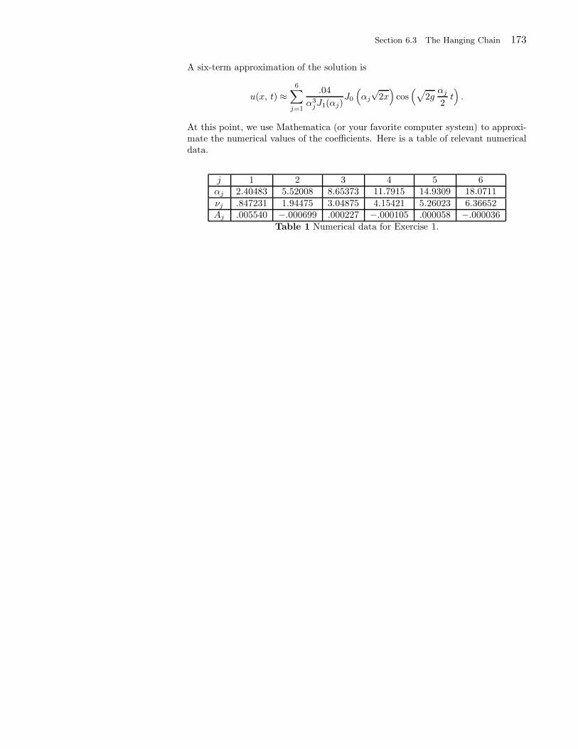
Section 6.3 The Hanging Chain 173
A six-term approximation of the solution is
u(x, t) ≈6∑
j=1
.04
α3jJ1(αj)
J0
(αj
√2x)
cos(√
2gαj
2t).
At this point, we use Mathematica (or your favorite computer system) to approxi-mate the numerical values of the coefficients. Here is a table of relevant numericaldata.
j 1 2 3 4 5 6αj 2.40483 5.52008 8.65373 11.7915 14.9309 18.0711
νj .847231 1.94475 3.04875 4.15421 5.26023 6.36652Aj .005540 −.000699 .000227 −.000105 .000058 −.000036
Table 1 Numerical data for Exercise 1.
174 Chapter 6 Sturm-Liouville Theory with Engineering Applications
Exercises 6.4
1. This is a special case of Example 1 with L = 2 and λ = α4. The values of αare the positive roots of the equation
cos 2α =1
cosh 2α.
There are infinitely many roots, αn (n = 1, 2, . . .), that can be approximated withthe help of a computer (see Figure 1). To each αn corresponds one eigenfunction
Xn(x) = coshαnx− cosαnx− cosh 2αn − cos 2αn
sinh 2αn − sin 2αn(sinhαnx− sinαnx) .
5. There are infinitely many eigenvalues λ = α4, where α is a positive root of theequation
cosα =1
coshα.
As in Example 1, the roots of this equation, αn (n = 1, 2, . . .), can be approxi-mated with the help of a computer (see Figure 1). To each αn corresponds oneeigenfunction
Xn(x) = coshαnx− cosαnx−coshαn − cosαn
sinhαn − sinαn(sinhαnx− sinαnx) .
The eigenfunction expansion of f(x) = x(1 − x), 0 < x < 1, is
f(x) =
∞∑
n=1
AnXn(x),
where
An ==
∫ 1
0x(1 − x)Xn(x) dx∫ 1
0X2
n(x) dx.
After computing several of these coefficients, it was observed that:
∫ 1
0
X2n(x) dx = 1 for all n = 1, 2, . . . ,
A2n = 0 for all n = 1, 2, . . . .
The first three nonzero coefficients are
A1 = .1788, A3 = .0331, A5 = .0134.
Sof(x) ≈ .1788X1(x) + .0331X3(x) + .0134X5(x),
where Xn described explicitely in Example 1. We have
X1(x) = cosh(4.7300 x)− cos(4.7300 x)+ .9825 (sin(4.7300 x)− sinh(4.7300 x)),
X2(x) = cosh(1.0008 x)− cos(1.0008 x)+ 1.0008 (sin(1.0008 x)− sinh(1.0008 x)),
X3(x) = cosh(10.9956 x)− cos(10.9956 x)+ sin(10.9956 x)− sinh(10.9956 x),
X4(x) = cosh(14.1372 x)− cos(14.1372 x)+ sin(14.1372 x)− sinh(14.1372 x),
X5(x) = cosh(17.2788 x)− cos(17.2788 x)+ sin(17.2788 x)− sinh(17.2788 x).
9. Assume that µ and X are an eigenvalue and a corresponding eigenfunction ofthe Sturm-Liouville problem
X′′ + µX = 0, X(0) = 0, X(L) = 0 .
Section 6.4 Fourth Order Sturm-Liouville Theory 175
Differentiate twice to see that X also satisfies the fourth order Sturm-Liouvilleproblem
X(4) − λX = 0,
X(0) = 0, X′′(0) = 0, X(L) = 0, X′′(L) = 0 .
If α and X are an eigenvalue and a corresponding eigenfunction of
X′′ + µX = 0, X(0) = 0, X(L) = 0,
then differentiating twice the equation, we find
X(4) + µX′′ = 0, X(0) = 0, X(L) = 0.
But X′′ = −µX, so X(4)−µ2X = 0 and hence X satisfies the equation X(4)−λX =0 with λ = µ2. Also, from X(0) = 0, X(L) = 0 and the fact that X′′ = −µX, itfollows that X′′(0) = 0 and X′′(L) = 0.
176 Chapter 6 Sturm-Liouville Theory with Engineering Applications
Exercises 6.6
1. uxxyy = 0, uxxxx = 4!, uyyyy = −4!, ∇4u = 0.
3. Let u(x, y) = xx2+y2 and v(x, y) = x · u(x, y). We know that u is harmonic
(Exercise 1, Section 4.1), and so v is biharmonic by Example 1, with A = 0, B = 1,C = D = 0.
5. Express v in Cartesian coordinates as follows:
v = r2 cos(2θ)(1 − r2)
= r2[cos2 θ − sin2 θ](1 − r2)
= (x2 − y2)(1 − (x2 + y2)
).
Let u = x2 − y2 . Then u is harmonic and so v is biharmonic by Example 1, withA = 1, D = 1, B = C = 0.
7. Write v = r2 · rn cosnθ and let u = rn cos nθ. Then u is harmonic (use theLaplacian in polar coordinates to check this last assertion) and so v is biharmonic,by Example 1 with A = 1 and B = C = D = 0.
9. Write v = ar2 ln r + br2 + c ln r + d = φ + ψ, where φ = [ar2 + c] ln r andψ = br2+d. From Example 1, it follows that ψ is biharmonic. Also, ln r is harmonic(check the Laplacian in polar coordinates) and so, by Example 1, φ is biharmonic.Consequently, v is biharmonic, being the sum of two biharmonic functions.
11. Since the boundary values are independent of θ, try for a solution a functionindependent of θ and of the form u = ar2 ln r + br2 + c ln r + d. We have
ur = 2ar ln r + ar + 2br +c
r= 2ar ln r + r(a+ 2b) +
c
r.
Now use the boundary conditions to solve for the unknown coefficients as follows:
u(1, θ) = 0 ⇒ b+ d = 0,
u(2, θ) = 0 ⇒ 4a ln 2 + 4b+ c ln 2 + d = 0,
ur(1, θ) = 1 ⇒ a+ 2b+ c = 1,
ur(2, θ) = 1 ⇒ 4a ln 2 + 2a+ 4b+c
2= 1.
Solving this system of four equations in four unknowns, we find
a =1
3 − 4 ln2, b =
−2 ln2
3 − 4 ln2, c =
2
3 − 4 ln2, d =
2 ln2
3 − 4 ln2,
and hence the solution
u(r, θ) =1
3 − 4 ln2
(r2 ln r − 2 ln(2)r2 + 2 ln r + 2 ln2
).
13. We follow the method of Theorem 1, as illustrated by Example 2. First, solvethe Dirichlet problem ∇2w = 0, w(1, θ) = cos 2θ, for 0 ≤ r < 1, 0 ≤ θ ≤ 2π.The solution in this case is w(r, θ) = r2 cos 2θ. (This is a simple application ofthe method of Section 4.4, since the boundary function is already given by itsFourier series.) We now consider a second Dirichlet problem on the unit disk withboundary values v(1, θ) = 1
2
(wr(1, θ) − g(θ)
). Since g(θ) = 0 and wr(r, θ) =
2r cos 2θ, it follows that v(1, θ) = cos 2θ. The solution of th Dirichlet problem in vis v(r, θ) = r2 cos 2θ. Thus the solution of biharmonic problem is
u(r, θ) = (1 − r2)r2 cos 2θ+ r2 cos 2θ = 2r2 cos 2θ − r4 cos 2θ.
Section 6.6 The Biharmonic Operator 177
This can be verified directly by plugging into the biharmonic equation and theboundary conditions.
15. We just give the answers details: w(r, θ) = 1, ∇2v = 0, v(1, θ) = 12(1− cos θ),
v(r, θ) = −12r cos θ; u(r, θ) = −1
2r cos θ(1 − r2) + 1.
17. u(1, 0) = 0 implies that w = 0 and so v(1, θ) = −g(θ)2
. So
v(r, θ) = −1
2
[a0 +
∞∑
n=1
rn(cos nθ+ bn sinnθ)],
where an and bn are the Fourier coefficients of g. Finally,
u(r, θ) = (1 − r2)v(r, θ) = −1
2(1 − r2)
[a0 +
∞∑
n=1
rn(cos nθ+ bn sinnθ)].
178 Chapter 6 Sturm-Liouville Theory with Engineering Applications
Exercises 6.7
12. Correction to the suggested proof: y2 = I0 and not J1.
15. Repeat Steps 1–3 of Example 2 without any change to arrive at the solution
u(r, t) =
∞∑
n=1
(αn cos(k2
nct) + βn sin(k2nct)
)φn(r),
where the kns are the positive roots of (16). Putting t = 0 we get 0 =∑∞
n=1 αnφn(r),which implies that αn = 0 for all n. Differentiating with respect to t then settingt = 0, we obtain
g(r) =
∞∑
n=1
k2ncβnφn(r),
which implies that
∫ 1
0
g(r)φn(r)r dr = k2ncβn
∫ 1
0
φ2n(r)r dr
or
βn =
∫ 1
0 g(r)φn(r)r dr
k2ncβn
∫ 1
0φ2
n(r)r dr.
The integral∫ 1
0 φ2n(r)r dr is given by (23).
17. Let u1(r, t) denote the solution of the problem in Example 3 and let u2(r, t)denote the solution in Example 3. Then, by linearity or superposition, u(r, t) =u1(r, t) + u2(r, t) is the desired solution.
19. Sketch of the solution:
u(r, t) =
∞∑
n=1
An(t)φn(r),
ut(r, t) =
∞∑
n=1
A′n(t)φn(r),
∇4u(r, t) =
∞∑
n=1
k4nAn(t)φn(r)
ut = −c2∇4u ⇒ A′n(t) = −c2k4
n
⇒ An(t) = Ane−c2k4
nt,
where An is a constant. So
u(r, t) =
∞∑
n=1
Ane−c2k4
ntφn(r).
Setting t = 0, we get, for 0 ≤ r < 1,
100 =
∞∑
n=1
Anφn(r).
Thus An is as in Example 1.
Section 7.1 The Fourier Integral Representation 179
Solutions to Exercises 7.1
1. We have
f(x) =
1 if −a < x < a, (a > 0)0 otherwise,
This problem is very similar to Example 1. From (3), if ω 6= 0, then
A(ω) =1
π
∫ ∞
−∞f(t) cos ωt dt =
1
π
∫ a
−a
cosωt dt =
[sinωt
πω
]a
−a
=2 sin aω
πω.
If ω = 0, then
A(0) =1
π
∫ ∞
−∞f(t) dt =
1
π
∫ a
−a
dt =2a
π.
Since f(x) is even, B(ω) = 0. For |x| 6= a the function is continuous and Theorem1 gives
f(x) =2a
π
∫ ∞
0
sin aω cosωx
ωdω .
For x = ±a, points of discontinuity of f , Theorem 1 yields the value 1/2 for thelast integral. Thus we have the Fourier integral representation of f
2a
π
∫ ∞
0
sin aω cosωx
ωdω =
1 if |x| < a,1/2 if |x| = a,0 if |x| > a.
3. We have
f(x) =
1 − cos x if −π/2 < x < π/2,0 otherwise.
The solution follows by combining Examples 1 and 2 and using the linearity of theFourier integral, or we can compute directly and basically repeat the computationin these examples. Since f is even, B(w) = 0 for all w, and
A(w) =2
π
∫ π/2
0
(1 − cos t
)coswt dt
=2 sin(πw/2)
πw− 2
π
∫ π/2
0
1
2[cos(w + 1)t+ cos(w − 1)t] dt
=2 sin(πw/2)
πw− 1
π
[sin(w + 1)t
w + 1+
sin(w − 1)t
w − 1
]∣∣∣∣π/2
0
(w 6= 1)
=2 sin(πw/2)
πw− 1
π
[sin(w + 1)π
2
w + 1+
sin(w − 1)π2
w − 1
](w 6= ±1)
=2 sin(πw/2)
πw− 1
π
[cos wπ
2
w + 1− cos wπ
2
w − 1
]
=2 sin(πw/2)
πw− 2
π
1
1 −w2cos
wπ
2,
If w = ±1,
A(w) =2 sin(±π/2)
±π − 2
π
∫ π/2
0
cos2 t dt
=2
π− 2
π
∫ π/2
0
1 + cos 2t
2dt =
2
π− 1
2.
(Another way to get this answer is to use the fact that A(w) is continuous (wheneverf is integrable) and take the limit of A(w) as w tends to ±1. You will get 1
2 .Applying the Fourier integral representation, we obtain:
2
π
∫ ∞
0
(sin(πw/2)
w− cos πw
2
1 −w2
)coswxdw = f(x) =
1 − cosx if |x| ≤ π
2 ,0 if |x| > π
2.
180 Chapter 7 The Fourier Transform and its Applications
5. since f(x) = e−|x| is even, B(w) = 0 for all w, and
A(w) =2
π
∫ ∞
0
e−t coswt dt
=2
π
e−t
1 +w2[− coswt+w sinwt]
∣∣∣∣∞
0
=2
π
1
1 +w2,
where we have used the result of Exercise 17, Sec. 2.6, to evaluate the integral.Applying the Fourier integral representation, we obtain:
e−|x| =2
π
∫ ∞
0
1
1 +w2coswx dw.
7. The function
f(x) =
1 if 0 < x < 1,0 otherwise,
is neither even nor odd. We will need to compute both A(w) and B(w). For w 6= 0,
A(w) =1
π
∫ 1
0
coswt dt =1
π
sinw
w;
B(w) =1
π
∫ 1
0
sinwt dt =1
π
1 − cosw
w.
If w = 0, just take limits ofA(w) and B(w) as w tends to 0. You will find: A(0) = 1π
and B(0) = 0. Thus we have the Fourier integral representation of f
1
π
∫ ∞
0
(sinw coswx+ (1 − cosw) sinwx
), dw =
0 if x < 0 or x > 1,1/2 if x = 0 or x = 1,1 if 0 < x < 1.
9. The function
f(x) =
x if −1 < x < 1,2 − x if 1 < x < 2,−2 − x if −2 < x < −1,0 otherwise,
is odd, as can be seen from its graph. Hence A(w) = 0 and
B(w) =2
π
∫ ∞
0
f(t) sinwt dt
=2
π
∫ 1
0
t sinwt dt+2
π
∫ 2
1
(2 − t) sinwt dt
=2
π
[−tw
coswt
∣∣∣∣1
0
+
∫ 1
0
coswt
wdt
]
+2
π
[−2 − t
wcoswt
∣∣∣∣2
1
+
∫ 2
1
coswt
wdt
]
=2
πw2[2 sinw − sin 2w] .
Since f is continuous, we obtain the Fourier integral representation of
f(x) =2
π
∫ ∞
0
1
w2[2 sinw − sin 2w] sinwx, dw.
11. For the function
f(x) =
sinx if 0 < x < π,0 otherwise,
Section 7.1 The Fourier Integral Representation 181
we have
A(w) =1
π
∫ π
0
sin t coswt dt
=1
2π
∫ π
0
[sin(1 +w)t+ sin(1 − w)t] dt
= − 1
2π
[cos(1 + w)t
1 +w+
cos(1 −w)t
1 −w
]∣∣∣∣π
0
(w 6= 1)
= − 1
2π
[cos(w + 1)π
1 +w+
cos(1 − w)π
1 −w− 1
1 + w− 1
1 − w
]
=1
2π
[coswπ
1 + w+
coswπ
1 − w+
2
1 − w2
]
=1
π(1 −w2)[coswπ + 1] .
B(w) =1
π
∫ π
0
sin t sinwt dt
= − 1
2π
∫ π
0
[cos(1 +w)t − cos(w − 1)t] dt
= − 1
2π
[sin(1 +w)t
1 +w− sin(1 −w)t
1 −w
]∣∣∣∣π
0
(w 6= 1)
= − 1
2π
[sin(w + 1)π
1 +w− sin(1 − w)π
1 − w
]
=sinwπ
π(1 −w2).
Thus the Fourier integral representation of f is
f(x) =1
π
∫ ∞
0
[1 + coswπ
1 − w2coswx+
sinwπ
1 − w2sinwx
]dx.
13. (a) Take x = 1 in the Fourier integral representation of Example 1:
2
π
∫ ∞
0
sinw cosw
wdw =
1
2⇒
∫ ∞
0
sinw cosw
wdw =
π
4.
(b) Integrate by parts: u = sin2 w, du = 2 sinw cosw dw, dv = 1w2 dw, v = − 1
w :
∫ ∞
0
sin2 ω
ω2dω =
=0︷ ︸︸ ︷sin2 w
w
∣∣∣∣∞
0
+2
∫ ∞
0
sinw cosw
w2dw =
π
2,
by (a).
15.
∫ ∞
0
sinω cos 2ω
ωdω = 0. Solution Just take x = 2 in Example 1.
17.∫ ∞
0
cosxω + ω sinxω
1 + ω2dω =
0 if x < 0,π/2 if x = 0,πe−x if x > 0.
Solution. Define
f(x) =
0 if x < 0,π/2 if x = 0,πe−x if x > 0.
182 Chapter 7 The Fourier Transform and its Applications
Let us find the Fourier integral representation of f :
A(w) =1
π
∫ ∞
0
πe−x coswx dx =1
1 +w2
(see Exercise 5);
B(w) =1
π
∫ ∞
0
πe−x sinwx dx =w
1 +w2,
(see Exercise 17, Sec. 2.6). So
f(x) =
∫ ∞
0
coswx+w sinwx
1 + w2dw,
which yields the desired formula.
19. Let f(x) = e−a|x|, where a > 0. Then f , satisfies the conditions of Theorem1, f is continuous and even. So it has a Fourier integral representation of the form
e−a |x| =
∫ ∞
0
A(w) coswx dx,
where
A(w) =2
π
∫ ∞
0
e−ax coswx dx
=2a
π(a2 + w2),
where the integral is evaluated with the help of Exercise 17, Sec. 2.6 (see Exercise5 of this section). For x ≥ 0, the Fourier integral representation becomes
e−ax =2a
π
∫ ∞
0
coswx
a2 +w2dw (x ≥ 0).
23. (a)
Si(−x) =
∫ −x
0
sin t
tdt
=
∫ x
0
sin(−u)(−u) (−1) du (Let u = −t.)
= −∫ x
0
sinu
udu = −Si(x).
Thus Si(x) is an odd function.(b) limx→−∞ Si(x) = limx→∞ −Si(x) − π
2, by (8).
(c) We have
sin t =
∞∑
n=0
(−1)n t2n+1
(2n+ 1)!−∞ < t <∞
sin t
t=
∞∑
n=0
(−1)n t2n
(2n+ 1)!−∞ < t <∞ (Divide by t.)
By a well-known property of power series, a power series may be integrated termby term within its radius of convergence. Here we are dealing with power seriesthat converge for all t; thus we may integrate them term by term on any interval.
Section 7.1 The Fourier Integral Representation 183
In particular, we have
Si(x) =
∫ x
0
sin t
tdt
=
∫ x
0
( ∞∑
n=0
(−1)n t2n
(2n+ 1)!
)dt
=
∞∑
n=0
(−1)n 1
(2n+ 1)!
∫ x
0
t2ndt
=∞∑
n=0
(−1)n 1
(2n+ 1)!
1
2n+ 1t2n+1
∣∣∣x
0
=
∞∑
n=0
(−1)n 1
(2n+ 1)!(2n+ 1)x2n+1.
25. We have
Si(a) =
∫ a
0
sin t
tdt, Si(b) =
∫ b
0
sin t
tdt.
So
Si(b) − Si(a) =
∫ b
0
sin t
tdt−
∫ a
0
sin t
tdt =
∫ b
a
sin t
tdt.
27. Let u = 1 − cosx, du = sinx, dv = 1x2 dx, v = − 1
x . Then
∫ b
a
1 − cos x
x2dx = −1 − cosx
x
∣∣∣∣b
a
+
∫ b
a
sinx
xdx
=cos b− 1
b− cos a− 1
a+ Si(b) − Si(a),
where we have used the result of Exercise 25.
184 Chapter 7 The Fourier Transform and its Applications
Solutions to Exercises 7.2
1. In computing f , the integral depends on the values of f on the interval (−1, 1).Since on this interval f is odd, it follows that f(x) coswx is odd and f(x) sinwx iseven on the interval (−1, 1). Thus
f(w) =1√2π
∫ ∞
−∞f(x)e−iwx dx
=1√2π
=0︷ ︸︸ ︷∫ 1
−1
f(x) coswx dx− i√2π
∫ 1
−1
f(x) sinwx dx
= − 2i√2π
∫ 1
0
sinwx dx
=2i√2π
coswx
w
∣∣∣1
0
= i
√2
π
cosw − 1
w.
3. We evaluate the Fourier transform with the help of Euler’s identity: e−iwx =coswx − i sinwx. We also use the fact that the integral of on odd function overa symmetric interval is 0, while the integral of an even function over a symmetricinterval [−a, a] is twice the integral over [0, a].
f(w) =1√2π
∫ ∞
−∞f(x)e−iwx dx
=1√2π
∫ π
−π
sinx(coswx− i sinwx) dx
=1√2π
=0︷ ︸︸ ︷∫ π
−π
sinx coswx dx− i√2π
∫ π
−π
sinx sinwx dx
= − 2i√2π
∫ π
0
1
2[(− cos(w + 1)x+ cos(w − 1)x] dx.
If w = 1,
f(1) = − i√2π
∫ π
0
[(− cos 2x+ 1] dx = − i√π√2.
If w = 1, we find similarly that
f(−1) =i√π√2.
(You may also note that f is odd in this case.) For w 6= ±1, we have
f(w) =i√2π
(1
w + 1sin(w + 1)x− 1
w − 1sin(w − 1)x)
∣∣∣∣π
0
=i√2π
( 1
w + 1sin(w + 1)π − 1
w − 1sin(w − 1)π
)
=i√2π
( 1
w + 1(−1) sinwπ − 1
w − 1(−1) sinwπ
)
=i√2π
sinwπ(− 1
w + 1+
1
w − 1
)
= i
√2
π
sinwπ
w2 − 1.
Section 7.2 The Fourier Transform 185
Check that as w → ±1, f(w) → f(±1).
5. Use integration by parts to evaluate the integrals:
f(w) =1√2π
∫ ∞
−∞f(x)e−iwx dx
=1√2π
∫ 1
−1
(1 − |x|)(coswx− i sinwx) dx
=1√2π
∫ 1
−1
(1 − |x|) coswx dx− i√2π
=0︷ ︸︸ ︷∫ 1
−1
(1 − |x|) sinwx dx
=2√2π
∫ 1
0
u︷ ︸︸ ︷(1 − x)
dv︷ ︸︸ ︷coswx dx
=2√2π
((1 − x)
sinwx
w
)∣∣∣∣1
0
+2√2πw
∫ 1
0
sinwx dx
= −√
2
π
coswx
w2
∣∣∣∣∣
1
0
=
√2
π
1 − cosw
w2.
7. Before we compute the transform, let us evaluate the integral
I =
∫xe−iwx dx (w 6= 0)
by parts. Let u = x, dv = e−iwx dx; then du = dx and v = 1−iwe
−iwx = iw e
−iwx,
because 1i = −i. So
∫xe−iwx dx = i
x
we−iwx − i
w
∫e−iwxdx = i
x
we−iwx +
1
w2e−iwx +C.
We are now ready to compute the transform. For w 6= 0, we have
f(w) =2√2π
∫ 10
0
xe−iwx dx
=2√2π
[ix
we−iwx +
1
w2e−iwx
]∣∣∣∣10
0
=
√2
π
[i10
we−10 iw +
e−10 iw − 1
w2
].
In terms of sines and cosine, we have
f(w) =
√2
π
[i10
w
(cos(10w) − i sin(10w)
)+
cos(10w)− i sin(10w) − 1
w2
]
=
√2
π
[10 sin(10w)
w+
cos(10w) − 1
w2+ i
(10 cos(10w)
w− sin(10w)
w2
)].
9. In Exercise 1,
f(0) =1√2π
× (area between graph of f(x) and the xaxis) = 0.
186 Chapter 7 The Fourier Transform and its Applications
In Exercise 7,
f(0) =1√2π
× (area between graph of f(x) and the xaxis) =100√2π.
11. We use the identity FF(f)(x) = f(−x). In case f is even, this identitybecomes FF(f)(x) = f(−x). Consider g(x) = 1
1+x2 and, for convenience, let us
write it as g(w) = 11+w2 . Recall from Exercise 5 that
F(e−|x|)(w) =
√2
π
1
1 + w2=
√2
πg(w).
Multiplying both sides by√
π2 and using the linearity of the Fourier transform, it
follows that
F(
√π
2e−|x|)(w) = g(w).
So
Fg = FF(√
π
2e−|x|
)=
√π
2e−|x|,
by the reciprocity relation. If we use the symbol w as a variable in the Fouriertransform, we get
F(
1
1 + x2
)=
√π
2e−|w|,
13. We argue as in Exercise 11. Consider g(x) = sin axx where we assume a > 0.
For the case a < 0, use sin(−ax) = − sin ax and linearity of the Fourier transform.Let f(x) = 1 if |x| < a and 0 otherwise. Recall from Example 1 that
F(f(x))(w) =
√2
π
sin aw
w=
√2
πg(w).
Multiplying both sides by√
π2 and using the linearity of the Fourier transform, it
follows that
F(
√π
2f(x))(w) = g(w).
So
Fg = FF(√
π
2f(x)
)=
√π
2f(x),
by the reciprocity relation. Using the symbol w as a variable, we get
F(
sin ax
x
)=
√π
2f(w) =
√π2 if |w| < a,
0 otherwise.
15. Consider the function in Example 2,
f(x) =
e−x if x > 0,
0 if x < 0.
If a > 0, then (see Exercise 17)
F(f(ax))(w) =1
a
1 − iw/a√2π(1 + (w/a)2)
=a− iw√
2π(a2 +w2).
But
f(ax) =
e−ax if x > 0,
0 if x < 0.
Section 7.2 The Fourier Transform 187
Hence
g(w) =a − iw
a2 +w2=
√2πF(f(ax))(w);
and so
F(g) =√
2πf(−ax) =
√2πeax if x < 0,
0 if x > 0.
Using the variable w,
F(g)(w) =
√2πeaw if w < 0,
0 if w > 0.
If a < 0, use the identity
F(f(−x))(w) = F(f(x))(−w)
(see Exercise 17 with a = −1) to conclude that
F(g)(w) =
√2πeaw if w > 0,
0 if w < 0.
17. (a) Consider first the case a > 0. Using the definition of the Fourier transformand a change of variables
F(f(ax))(w) =1√2π
∫ ∞
−∞f(ax)e−iωx dx
=1
a
1√2π
∫ ∞
−∞f(x)e−i ω
a x dx (ax = X, dx =1
adX)
=1
aF(f)(
w
a).
If a < 0, then
F(f(ax))(w) =1√2π
∫ ∞
−∞f(ax)e−iωx dx
=1
a
1√2π
∫ −∞
∞f(x)e−i ω
a x dx
= −1
aF(f)(
w
a).
Hence for all a 6= 0, we can write
=1
|a| F(f)(ωa
).
(b) We have
F(e−|x|)(w) =
√2
π
1
1 +w2.
By (a),
F(e−2|x|)(w) =1
2
√2
π
1
1 + (w/2)2=
√2
π
2
4 +w2.
(c) Let f(x) denote the function in Example 2. Then g(x) = f(−x). So
g(w) = f(−w) =1 + iw√
2π(1 +w2).
Let h(x) = e−|x|. Then h(x) = f(x) + g(x). So
h(w) = f(w) + g(w) =1 − iw√
2π(1 +w2)+
1 + iw√2π(1 + w2)
=
√2
π
1
1 + w2.
188 Chapter 7 The Fourier Transform and its Applications
19. Using the definition of the Fourier transform
F(f(x − a))(w) =1√2π
∫ ∞
−∞f(x − a)e−iωx dx
=1√2π
∫ ∞
−∞f(x)e−iω(x+a) dx (x− a = X, dx = dX)
= e−iωa 1√2π
∫ ∞
−∞f(x)e−iωx dx = e−iaωF(f)(ω).
21. We have F(e−x2
) = 1√2e−w2/4, by Theorem 5. Using Exercise 20, we have
F(cosx
ex2 ) = F(cos xe−x2
)
=1
2√
2
(e−
(w−a)2
4 + e−(w+a)2
4
)
23. We have F( 11+x2 ) =
√π2 e
−|w|. Using Exercise 20, we have
F(cosx+ cos 2x
1 + x2) = F(
cos x
1 + x2) + F(
cos 2x
1 + x2)
=1
2
√π
2
(e−|w−1| + e−|w+1| + e−|w−2| + e−|w+2|
).
25 Let
g(x) =
1 if |x| < 1,0 otherwise,
and note that f(x) = cos(x) g(x). Now F(g(x)) =√
2π
sin ww . Using Exercise 20, we
have
F(f(x)) = F(cos xg(x))
=1
2
√2
π
(sin(w − 1)
w − 1+
sin(w + 1)
w + 1
).
27. Call g(x) the function in the figure. The support of g is the interval (a, b), thathas length b − a. Translate the function by b+a
2in order to center its support at
the origin, over the interval with endpoints at(− b−a
2, b−a
2
). Denote the translated
function by f(x). Thus, g(x) = f(x− b+a
2
), where f(x) = h if |x| < b−a
2 and 0otherwise. By Example 1 and Exercise 19,
g(w) = e−i b+a2 wf(w)
= e−i b+a2 wh ·
√2
π
sin(
b−a2w)
w
=
√2
πhe−i b+a
2 w sin(
b−a2 w
)
w.
29. Take a = 0 and relabel b = a in Exercise 27, you will get the function f(x) = hif 0 < x < a. Its Fourier transform is
f(w) ==
√2
πhe−i a
2 w sin(
a w2
)
w.
Section 7.2 The Fourier Transform 189
Let g(x) denote the function in the figure. Then g(x) = 1ax f(x) and so, by Theo-
rem 3,
g(w) =1
aid
dwf(w)
= i
√2
π
h
a
d
dw
[e−i a
2 w sin(
a w2
)
w
]
= i
√2
π
h
a
e−i a2 w
w
[acos(
a w2
)− i sin
(a w2
)
2− sin
(a w2
)
w
]
= i
√2
π
h
ae−i a
2 w
[−2 sin
(a w2
)+ aw e−i a
2 w
2w2
].
31. Let f(x) = 1 if −a < x < a and 0 otherwise (Example 1), and let g(x) denotethe function in the figure. Then g(x) = x2f(x) and, by Theorem 3,
g(w) = − d2
dw2f(w)
= −√
2
π
d2
dw2
sin aw
w
= −√
2
π
2aw cos aw + a2w2 sinaw − 2 sin aw
w3.
33. Let g(x) denote the function in this exercise. By the reciprocity relation, sincethe function is even, we have F(F(g)) = g(−x) = g(x). Taking inverse Fouriertransforms, we obtain F−1(g) = F(g). Hence it is enough to compute the Fouriertransform. We use the notation and the result of Exercise 34. We have
g(x) = 2f2a(x) − fa(x).
Verify this identity by drawing the graphs of f2a and fa and then drawing the graphof f2a(x) − fa(x). With the help of this identity and the result of Exercise 34, wehave
g(w) = 2f2a(w) − fa(w)
= 28a√2π
sin2 (aw)
4(aw)2− 4a√
2π
sin2(
aw2
)
(aw)2
=4
a√
2π
[sin2 (aw)
w2− sin2
(aw2
)
w2
].
35. (a) Apply Theorem 5 with a = 2, then
F(e−x2
) =1√2e−w2/4.
37. By Exercise 27,
F(e−x2
) =1√2e−w2/4.
190 Chapter 7 The Fourier Transform and its Applications
By Theorem 3(i)
F(xe−x2
) = id
dw
( 1√2e−w2/4
)
=i
2√
2e−w2/4.
39. Let
g(x) =
1 if |x| < 1,0 otherwise,
and note that f(x) = xg(x). Now F(g(x)) =√
2π
sin ww . By Theorem 3(i)
F(f(x)) = F(xg(x))
= id
dw
(√ 2
π
sinw
w
)
= i
√2
π
w cosw − sinw
w2.
41. We have F( 11+x2 ) =
√π2 e
−|w|. So if w > 0
F(x
1 + x2)(w) = i
√π
2
d
dwe−w = −i
√π
2e−w.
If w < 0
F(x
1 + x2)(w) = i
√π
2
d
dwew = i
√π
2ew .
If w = 0,
F(x
1 + x2)(0) =
1√2π
∫ ∞
−∞
x
1 + x2dx = 0
(odd integrand). We can combine these answers into one formula
F(x
1 + x2)(w) = −i
√π
2sgn (w)e−|w|.
43. Using linearity,
F((1 − x2)e−x2
)= F
(e−x2
)−F
(x2e−x2
).
By Theorem 3(ii) and Exercise 27,
F((1 − x2)e−x2
)=
1√2e−w2/4 +
1√2
d2
dw2e−w2/4
=1
4√
2e−w2/4
(2 +w2
).
45. Theorem 3 (i) and Exercise 19:
F(xe−12 (x−1)2) = i
d
dw
(F(e−
12 (x−1)2)
)
= id
dw
(e−iwF(e−
12x2
))
= id
dw
(e−iwe−
12w2
))
= id
dw
(e−
12 w2−iw)
)
= i(−w − i)e−12w2−iw
= (1 − iw)e−12w2−iw.
Section 7.2 The Fourier Transform 191
49.
h(ω) = e−ω2 · 1
1 + ω2= F
( 1√2e−x2/4
)· F(√π
2e−|x|).
Hence
h(x) = f ∗ g(x) =1√2π
∫ ∞
−∞
1√2e−
(x−t)2
4
√π
2e−|t|dt
=1
2√
2
∫ ∞
−∞e−
(x−t)2
4 e−|t|dt.
51. Let
f(ω) =
1 if |ω| < 1,0 otherwise.
Thenh(ω) = f(ω)e−
12ω2
.
We have F−1(e−12ω2
) = e−12x2
and f(x) =√
2π
sin xx
. Thus
h(x) = f ∗ g(x) =1√2π
∫ ∞
−∞e−
(x−t)2
2
√2
π
sin t
tdt
=1
π
∫ ∞
−∞e−
(x−t)2
2sin t
tdt.
53. Let f(x) = xe−x2/2 and g(x) = e−x2
.
(a) F(f)(w) = −iwe− w2
2 , and F(g)(w) = 1√2e−
w2
4 .
(b)
∗ = · = −i w√
2e−
w2
4 e−w2
2
= −i w√2e−3 w2
4 .
(c) With the help of Theorem 3
f ∗ g = F−1(− i
w√2e−3w2
4
)
= F−1(i
1√2
4
6
d
dwe−3 w2
4
)
=1√2
2
3F−1
(id
dwe−3 w2
4
)=
1√2
2
3xF−1
(e−3 w2
4
)
=2
3√
3xe−
13x2
.
In computing F−1(e−3 w2
4
), use Exercise 10(a) and (5) to obtain
F−1(e−aw2
)=
1√2ae−
(−x)2
4a =1√2ae−
x2
4a .
55. We use the uniqueness of the Fourier transform, which states that if h = kthen h = k.(a) Let h = f ∗ g and k = g ∗ f and use Theorem 4. Then
F(h) = F(f) · F(g) = F(g) · F(f) = F(g ∗ f).
192 Chapter 7 The Fourier Transform and its Applications
hence f ∗ g = g ∗ f .(b) Let u = f ∗ (g ∗ h) and v = (f ∗ g) ∗ h. Then
F(u) = F(f) · F(g ∗ h) = F(f) · (F(g) · F(h))
= (F(f) · F(g)) · F(h) = F(f ∗ g) · F(h)
= F((f ∗ g) ∗ h) = F(v).
Hence u = v or f ∗ (g ∗ h) = (f ∗ g) ∗ h).(c) Use Exercise19:
F(fa) = F(f(x − a)) = e−iawF(f).
So
F((f ∗ g)a) = F(f ∗ g(x − a)) = e−iawF(f ∗ g)
=
F(fa)︷ ︸︸ ︷e−iawF(f)F(g) = F(fa)F(g) = F(fa ∗ g).
Thus (f ∗ g)a = fa ∗ g. Similarly, (f ∗ g)a = f ∗ (ga).
57. Recall that f is integrable means that
∫ ∞
−∞|f(x)| dx <∞.
If f and g are integrable, then
f ∗ g(x) =1√2π
∫ ∞
−∞f(x − t)g(t) dt.
So, using properties of the integral:
∫ ∞
−∞|f ∗ g(x)|dx =
∫ ∞
−∞
∣∣∣∣1√2π
∫ ∞
−∞f(x − t)g(t) dt
∣∣∣∣ dx
≤ 1√2π
∫ ∞
−∞
∫ ∞
−∞|f(x− t)g(t)| dx dt
(Interchange order of integration.
≤ 1√2π
∫ ∞
−∞
=R ∞−∞|f(x)|dx
︷ ︸︸ ︷∫ ∞
−∞|f(x− t)| dx |g(t)| dt
(Change variables in the inner integral X = x− t.)
≤ 1√2π
∫ ∞
−∞|f(x)| dx
∫ ∞
−∞|g(t)| dt <∞;
thus f ∗ g is integrable.
Section 7.3 The Fourier Transform Method 193
Solutions to Exercises 7.3
1.
∂2u
∂t2=∂2u
∂x2,
u(x, 0) =1
1 + x2,
∂u
∂t(x, 0) = 0.
Follow the solution of Example 1. Fix t and Fourier transform the problem withrespect to the variable x:
d2
dt2u(w, t) = −w2u(w, t),
u(w, 0) = F( 1
1 + x2
)=
√π
2e−|w|,
d
dtu(w, 0) = 0.
Solve the second order differential equation in u(w, t):
u(w, t) = A(w) coswt+B(w) sinwt.
Using ddt u(w, 0) = 0, we get
−A(w)w sinwt+ B(w)w coswt∣∣∣t=0
= 0 ⇒ B(w)w = 0 ⇒ B(w) = 0.
Hence
u(w, t) = A(w) coswt.
Using u(w, 0) =√
π2e−|w|, we see that A(w) =
√π2e−|w| and so
u(w, t) =
√π
2e−|w| coswt.
Taking inverse Fourier transforms, we get
u(x, t) =
∫ ∞
−∞e−|w| coswt eixw dw.
3.
∂u
∂t=
1
4
∂2u
∂x2,
u(x, 0) = e−x2
.
Fix t and Fourier transform the problem with respect to the variable x:
d
dtu(w, t) = −w
2
4u(w, t),
u(w, 0) = F(e−x2)
=1√2e−
w2
4 .
Solve the first order differential equation in u(w, t):
u(w, t) = A(w)e−w2
4 .
Using u(w, 0) = 1√2e−
w2
4 , we get A(w) = 1√2e−
w2
4 . Hence
u(w, t) =1√2e−
w2
4 e−w2
4 t =1√2e−
w2
4 (1+t).
194 Chapter 7 The Fourier Transform and its Applications
Taking inverse Fourier transforms, we get
u(x, t) =1
2√π
∫ ∞
−∞e−
w2
4 (1+t) eixw dw.
5.
∂2u
∂t2= c2
∂2u
∂x2,
u(x, 0) =
√2
π
sinx
x,
∂u
∂t(x, 0) = 0.
Fix t and Fourier transform the problem with respect to the variable x:
d2
dt2u(w, t) = −c2w2u(w, t),
u(w, 0) = F(√
sinx
x
)(w) = f(w) =
1 if |w| < 10 if |w| > 1,
d
dtu(w, 0) = 0.
Solve the second order differential equation in u(w, t):
u(w, t) = A(w) cos cwt+B(w) sin cwt.
Using ddt u(w, 0) = 0, we get
u(w, t) = A(w) cos cwt.
Using u(w, 0) = f(w), we see that
u(w, t) = f(w) coswt.
Taking inverse Fourier transforms, we get
u(x, t) =1√2π
∫ ∞
−∞f(w) cos cwt eixw dw =
1√2π
∫ 1
−1
cos cwt eixw dw.
7.
∂u
∂x+ 3
∂u
∂t= 0,
u(x, 0) = f(x) .
Fourier transform the problem with respect to the variable x:
d
dtu(w, t) = − iw
3u(w, t),
u(w, 0) = F(u(x, 0)
)(w) = f(w).
Solve the first order differential equation in u(w, t):
u(w, t) = A(w)e−i w3 t.
Using the transformed initial condition, we get
u(w, t) = f(w)e−i w3 t.
Taking inverse Fourier transforms, we get
u(x, t) =1√2π
∫ ∞
−∞f(w)e−i w
3 t eixw dw =1√2π
∫ ∞
−∞f(w)eiw(x− t
3 ) dw = f(x − t
3).
Section 7.3 The Fourier Transform Method 195
9.
t2∂u
∂x− ∂u
∂t= 0,
u(x, 0) = 3 cosx .
The solution of this problem is very much like the solution of Exercise 7. However,there is a difficulty in computing the Fourier transform of cos x, because cosx is notintegrable on the real line. One can make sense of the Fourier transform by treatingcosx as a generalized function, but there is no need for this in this solution, sincewe do not need the exact formula of the Fourier transform, as you will see shortly.
Let f(x) = 3 cosx and Fourier transform the problem with respect to thevariable x:
t2iwu(w, t) − d
dtu(w, t) = 0,
u(w, 0) = F(3 cosx)
)(w) = f(w).
Solve the first order differential equation in u(w, t):
u(w, t) = A(w)e−i w3 t3 .
Using the transformed initial condition, we get
u(w, t) = f(w)e−i w3 t3.
Taking inverse Fourier transforms, we get
u(x, t) =1√2π
∫ ∞
−∞f(w)e−i w
3 t3 eixw dw
=1√2π
∫ ∞
−∞f(w)eiw(x+ t3
3 ) dw
= f(x+t3
3) = 3 cos(x+
t3
3).
11.
∂u
∂x=∂u
∂t,
u(x, 0) = f(x) .
Fourier transform the problem with respect to the variable x:
d
dtu(w, t) − iwu(w, t) = 0,
u(w, 0) = f(w).
Solve the first order differential equation in u(w, t):
u(w, t) = A(w)eiwt.
Using the transformed initial condition, we get
u(w, t) = f(w)eiwt.
Taking inverse Fourier transforms, we get
u(x, t) =1√2π
∫ ∞
−∞f(w)e−iwt eixw dw
=1√2π
∫ ∞
−∞f(w)eiw(x+t) dw
= f(x + t).
196 Chapter 7 The Fourier Transform and its Applications
13.
∂u
∂t= t
∂2u
∂x2,
u(x, 0) = f(x) .
Fix t and Fourier transform the problem with respect to the variable x:
d
dtu(w, t) + tw2u(w, t) = 0,
u(w, 0) = f(w).
Solve the first order differential equation in u(w, t):
u(w, t) = A(w)e−t2w2
2 .
Use the initial condition: A(w) = f(w). Hence
u(w, t) = f(w)e−t2w2
2 .
Taking inverse Fourier transforms, we get
u(x, t) =1√2π
∫ ∞
−∞f(w)e−
t2w2
2 eixw dw.
15.
∂2u
∂t2+ 2
∂u
∂t= −u,
u(x, 0) = f(x), ut(x, 0) = g(x) .
Fourier transform the problem with respect to the variable x:
d2
dt2u(w, t) + 2
d
dtu(w, t) + u(w, t) = 0,
u(w, 0) = f(w), .d
dtu(w, t) = g(w).
Solve the second order differential equation in u(w, t). The characteristic equationis λ2 + 2λ + 1 = 0. Since we have a repeated root λ = −1, the general solution isof the form:
u(w, t) = A(w)e−t +B(w)te−t.
The initial condition u(w, 0) = f(w) implies that f(w) = A(w). So u(w, t) =
f(w)e−t +B(w)te−t. The condition ddtu(w, t) = g(w) implies that −f(w)+B(w) =
g(w) or B(w) = f(w) + g(w). So
u(w, t) = f(w)e−t + (f(w) + g(w))te−t.
Hence Taking inverse Fourier transforms, we get
u(x, t) =1√2π
∫ ∞
−∞
(f(w)e−t + (f(w) + g(w))te−t
)eixw dw
= e−t 1√2π
∫ ∞
−∞f(w) eixw dw + te−t 1√
2π
∫ ∞
−∞
(f(w) + g(w)
)eixw dw
= e−tf(x) + te−t(f(x) + g(x).
17.
∂2u
∂t2=∂4u
∂x4
u(x, 0) =
100 if |x| < 2,0 otherwise.
Section 7.3 The Fourier Transform Method 197
Fourier transform the problem with respect to the variable x:
d2
dt2u(w, t) = w4u(w, t),
u(w, 0) = f(w) = 100
√2
π
sin 2w
w.
Solve the second order differential equation in u(w, t):
u(w, t) = A(w)e−w2t + B(w)ew2t.
Because a Fourier transform is expected to tend to 0 as w → ±∞, if we fix t > 0and let w → ∞ or w → −∞, we see that one way to make u(w, t) → 0 is to take
B(w) = 0. Then u(w, t) = A(w)e−w2t, and from the initial condition we obtain
B(w) = f(w). So
u(w, t) = f(w)e−w2t = 100
√2
π
sin 2w
we−w2t.
Taking inverse Fourier transforms, we get
u(x, t) =1√2π
∫ ∞
−∞100
√2
π
sin 2w
we−w2t eixw dw
=100
π
∫ ∞
−∞
sin 2w
we−w2t eixw dw.
19.
∂2u
∂t2=
∂3u
∂t∂x2,
u(x, 0) = f(x), ut(x, 0) = g(x) .
Fourier transform the problem with respect to the variable x:
d2
dt2u(w, t) = −w2 d
dtu(w, t),
u(w, 0) = f(w),d
dtu(w, 0) = g(w).
Solve the second order differential equation in u(w, t). The characteristic equationis λ2 +w2λ = 0, with roots λ = 0 or λ = −w2. The general solution is of the form:
u(w, t) = A(w) +B(w)e−w2t.
The initial condition u(w, 0) = f(w) implies that f(w) = A(w) +B(w) or A(w) =
f(w) − B(w). So
u(w, t) = f(w) +B(w)(e−w2t − 1).
The condition ddt u(w, 0) = g(w)
g(w) = −B(w)w2 ⇒ B(w) = − g(w)
w2.
So
u(w, t) = u(w, t) = f(w) − g(w)
w2(e−w2t − 1) = f(w) +
g(w)
w2(1 − e−w2t).
Taking inverse Fourier transforms, we get
u(x, t) =1√2π
∫ ∞
−∞
(f(w) +
g(w)
w2(1 − e−w2t)
)eixw dw
=1√2π
∫ ∞
−∞f(w) eixw dw +
1√2π
∫ ∞
−∞
g(w)
w2(1 − e−w2t)
)eixw dw
= f(x) +1√2π
∫ ∞
−∞
g(w)
w2(1 − e−w2t)
)eixw dw.
198 Chapter 7 The Fourier Transform and its Applications
21. (a) To verify that
u(x, t) =1
2[f(x− ct) + f(x + ct)] +
1
2c
∫ x+ct
x−ct
g(s) ds
is a solution of the boundary value problem of Example 1 is straightforward. Youjust have to plug the solution into the equation and the initial and boundary con-ditions and see that the equations are verified. The details are sketched in Section3.4, following Example 1 of that section.(b) In Example 1, we derived the solution as an inverse Fourier transform:
u(x, t) =1√2π
∫ ∞
−∞
[f(w) cos cwt+
1
cwg(w) sin cwt
]eiwx dx.
Using properties of the Fourier transform, we will show that
1√2π
∫ ∞
−∞f(w) cos cwteiwx dw =
1
2[f(x− ct) + f(x + ct)];(1)
1√2π
∫ ∞
−∞
1
wg(w) sin cwt eiwx dw =
1
2
∫ x+ct
x−ct
g(s) ds.(2)
To prove (1), note that
cos cwt =eicwt + e−icwt
2,
so
1√2π
∫ ∞
−∞f(w) cos cwteiwx dw
=1√2π
∫ ∞
−∞f(w) (
eicwt + e−icwt
2)eiwx dw
=1
2
[1√2π
∫ ∞
−∞f(w) eiw(x+ct) dw
1√2π
∫ ∞
−∞f(w) eiw(x−ct) dw
]
=1
2[f(x+ ct) + f(x − ct)];
because the first integral is simply the inverse Fourier transform of f evaluated atx + ct, and the second integral is the inverse Fourier transform of f evaluated atx− ct. This proves (1). To prove (2), we note that the left side of (2) is an inverseFourier transform. So (2) will follow if we can show that
(3) F∫ x+ct
x−ct
g(s) ds
=
2
wg(w) sin cwt.
Let G denote an antiderivative of g. Then (3) is equivalent to
F (G(x+ ct) −G(x− ct)) (w) =2
wG′(w) sin cwt.
Since G′ = iwG, the last equation is equivalent to
(4) F (G(x+ ct)) (w) − F (G(x− ct)) (w) = 2iG(w) sin cwt.
Using Exercise 19, Sec. 7.2, we have
F (G(x+ ct)) (w) −F (G(x− ct)) (w) = eictwF(G)(w) − e−ictwF(G)(w)
= F(G)(w)(eictw − e−ictw
)
= 2iG(w) sin cwt,
Section 7.3 The Fourier Transform Method 199
where we have applied the formula
sin ctw =eictw − e−ictw
2i.
This proves (4) and completes the solution.
23. Fourier transform the boundary value problem
∂u
∂t= c2
∂2u
∂x2+ k
∂u
∂x, −∞ < x <∞, t > 0,
u(x, 0) = f(x) ,
and get
d
dtu(w, t) = −c2w2 u(w, t) + ikwu(w, t) = u(w, t)(−c2w2 + ikw),
u(w, 0) = f(w).
Solve the first order differential equation in u(w, t) and get
u(w, t) = A(w)e(−c2w2+ikw)t.
The initial condition u(w, 0) = f(w) implies
u(w, t) = f(w)e(−c2w2+ikw)t.
Taking inverse Fourier transforms, we get
u(x, t) =1√2π
∫ ∞
−∞f(w)e(−c2w2+ikw)t eixw dw
=1√2π
∫ ∞
−∞f(w)e−c2w2t eiw(x+kt) dw.
25. Using the Fourier transform, we obtain
d2
dt2u(w, t) = c2 w4u(w, t),
u(w, 0) = f(w),d
dtu(w, 0) = g(w) .
Thusu(w, t) = A(w)e−cw2t + B(w)ecw2t.
Using the initial conditions:
u(w, 0) = f(w) ⇒ A(w) + B(w) = f(w) ⇒ A(w) = f(w) −B(w);
and
d
dtu(w, 0) = g(w) ⇒ −cw2A(w) + cw2B(w) = g(w)
⇒ −A(w) +B(w) =g(w)
cw2
⇒ −f(w) + 2B(w) =g(w)
cw2
⇒ B(w) =1
2
(f(w) +
g(w)
cw2
);
⇒ A(w) =1
2
(f(w) − g(w)
cw2
).
200 Chapter 7 The Fourier Transform and its Applications
Hence
u(w, t) =1
2
(f(w) − g(w)
cw2
)e−cw2t +
1
2
(f(w) +
g(w)
cw2
)ecw2t.
= f(w)(ecw2t + e−cw2t)
2+g(w)
cw2
(ecw2t − e−cw2t)
2
= f(w) cosh(cw2t) +g(w)
cw2sinh(cw2t)
Taking inverse Fourier transforms, we get
u(x, t) =1√2π
∫ ∞
−∞
(f(w) cosh(cw2t) +
g(w)
cw2sinh(cw2t)
)eixw dw.
27. Fourier transform the boundary value problem:
d
dtu(w, t) = −ic2w3 u(w, t),
u(w, 0) = f(w).
Solve the equation in u(w, t):
u(w, t) = A(w)e−ic2w3t.
Apply the initial condition:
u(w, t) = f(w)e−ic2w3t.
Inverse Fourier transform:
u(x, t) =1√2π
∫ ∞
−∞f(w)e−ic2w3t eixw dw.
Section 7.4 The Heat Equation and Gauss’s Kernel 201
Solutions to Exercises 7.4
1. Repeat the solution of Example 1 making some adjustments: c = 12 , gt(x) =
√2√te−
x2
t ,
u(x, t) = f ∗ gt(x)
=1√2π
∫ ∞
−∞f(s)
√2√te−
(x−s)2
t ds
=20√tπ
∫ 1
−1
e−(x−s)2
t ds (v =x− s√
t, dv = − 1√
tds)
=20√π
∫ x+1√t
x−1√t
e−v2
ds
= 10
(erf(
x+ 1√t
) − erf(x− 1√
t)
).
3. Let us use an approach similar to Example 2. Fourier transform the boundaryvalue problem and get:
d
dtu(w, t) = −w2u(w, t)
u(w, 0) = F(70e−x2
2 ) = 70e−w2
2 .
Solve the equation in u:
u(w, t) = A(w)e−w2t.
Apply the boundary condition:
u(w, t) = 70e−w2
2 )e−w2t = 70e−w2(t+ 12 ).
Inverse Fourier transform:
u(x, t) = F−1(70e−w2(t+ 1
2 ))
(1
2a= t+
1
2)
=70√
2t+ 1F−1
(√2t+ 1e−
w2
2a
)(a =
1
2t+ 1)
=70√
2t+ 1e−
x2
2(2t+1) ,
where we have used Theorem 5, Sec. 7.2.
5. Apply (4) with f(s) = s2:
u(x, t) = f ∗ gt(x)
=1√2t
1√2π
∫ ∞
−∞s2e−
(x−s)2
t ds.
You can evaluate this integral by using integration by parts twice and then appealingto Theorem 5, Section 7.2. However, we will use a different technique based on theoperational properties of the Fourier transform that enables us to evaluate a muchmore general integral. Let n be a nonnegative integer and suppose that f andsnf(s) are integrable and tend to 0 at ±∞. Then
1√2π
∫ ∞
−∞snf(s) ds = (i)n
[dn
dwnF(f)(w)
]
w=0
.
This formula is immediate if we recall Theorem 3(ii), Section 7.2, and that
φ(0) =1√2π
∫ ∞
−∞φ(s) ds.
202 Chapter 7 The Fourier Transform and its Applications
We will apply this formula with
f(s) =1√2te−
(x−s)2
t .
We have
F(
1√2te−
(x−s)2
t
)(w) = e−iwxF
(1√2te−
s2
t
)(w) (by Exercise 19, Sec. 7.2)
= e−iwxe−w2t = e−(iwx+w2t) (See the proof of Th. 1.)
So
u(x, t) =1√2t
1√2π
∫ ∞
−∞s2e−
(x−s)2
t ds
= −[d2
dw2F(
1√2te−
(x−s)2
t
)(w)
]
w=0
= −[d2
dw2e−(iwx+w2t)
]
w=0
= −[d
dw− e−(iwx+w2t)(ix + 2wt)
]
w=0
=[−e−(iwx+w2t)(ix+ 2wt)2 + 2te−(iwx+w2t)
]
w=0
= x2 + 2t.
You can check the validity of this answer by plugging it back into the heat equation.The initial condition is also obviously met: u(x, 0) = x2.
The approach that we took can be used to solve the boundary value problemwith f(x)xn as initial temperature distribution. See the end of this section forinteresting applications.
7. Proceed as in Example 2. Fourier transform the problem:
du
dtu(w, t) = −t2w2u(w, t), u(w, 0) = f(w).
Solve for u(w, t):
u(w, t) = f(w)e−w2 t3
3 .
Inverse Fourier transform and note that
u(x, t) = f ∗ F−1(e−w2 t3
3
).
With the help of Theorem 5, Sec. 7.2 (take a = t3
3 ), we find
F−1(e−w2 t3
3
)=
√3√
2t3e−x2 3
4t3 .
Thus
u(x, t) =1√2π
∫ ∞
−∞f(s)
√3√
2t3e−
3(x−s)2
4t3 ds
=
√3
2√πt3
∫ ∞
−∞f(s)e−
3(x−s)2
4t3 ds.
9. Fourier transform the problem:
du
dtu(w, t) = −e−tw2u(w, t), u(w, 0) = f(w).
Section 7.4 The Heat Equation and Gauss’s Kernel 203
Solve for u(w, t):
u(w, t) = f(w)e−w2(1−e−t).
Inverse Fourier transform and note that
u(x, t) = f ∗ F−1(e−w2(1−e−t)
).
With the help of Theorem 5, Sec. 7.2 (take a = 1 − e−t), we find
F−1(e−w2(1−e−t)
)=
1√2√
1 − e−te− x2
4(1−e−t ) .
Thus
u(x, t) =1
2√π√
1 − e−t
∫ ∞
−∞f(s)e
− (x−s)2
4(1−e−t) ds.
11. This is a generalization of Exercise 9 that can be solved by similar methods.Fourier transform the problem:
du
dtu(w, t) = −a(t)w2u(w, t), u(w, 0) = f(w).
Let B(t) denote an antiderivative of a(t), hence B(t) =∫ t
0a(τ ) dτ . Then u(w, t):
u(w, t) = f(w)e−w2B(t).
Inverse Fourier transform and note that
u(x, t) = f ∗ F−1(e−w2B(t)
).
With the help of Theorem 5, Sec. 7.2 (take a = B(t)), we find
F−1(e−w2B(t)
)=
1√2B(t)
e−x2
4B(t) .
Thus
u(x, t) =1
2√πB(t)
∫ ∞
−∞f(s)e−
(x−s)2
4B(t) ds.
13. If in Exercise 9 we take
f(x) =
100 if |x| < 1,0 otherwise,
then the solution becomes
u(x, t) =50√
π√
1− e−t
∫ 1
−1
e− (x−s)2
4(1−e−t) ds.
Let z = x−s2√
1−e−t , dz = −ds2√
1−e−t . Then
u(x, t) =50√
π√
1 − e−t2√
1 − e−t
∫ x+1
2√
1−e−t
x−1
2√
1−e−t
e−z2
dz
=100√π
∫ x+1
2√
1−e−t
x−1
2√
1−e−t
e−z2
dz
= 50
[erf
(x+ 1
2√
1 − e−t
)− erf
(x− 1
2√
1 − e−t
)].
204 Chapter 7 The Fourier Transform and its Applications
As t increases, the expression erf(
x+12√
1−e−t
)−erf
(x−1
2√
1−e−t
)approaches very quickly
erf(
x+12
)− erf
(x−1
2
), which tells us that the temperature approaches the limiting
distribution
50
[erf
(x+ 1
2
)− erf
(x− 1
2
)].
You can verify this assertion using graphs.
15. (a) From the definition
erf(−x) =2√π
∫ −x
0
e−z2
dz
= − 2√π
∫ x
0
e−(−z)2 dz (z = −Z, dz = −dZ)
= −erf(x)
Thus erf is an odd function.(b) From the definition
erf(0) =2√π
∫ 0
0
e−z2
dz = 0,
erf(∞) =2√π
∫ ∞
0
e−z2
dz = 1,
by (4)m Sec. 4.2.(c) By the fundamental theorem of calculus,
d
dxerf(x) =
2√π
d
dx
∫ x
0
e−z2
dz
=2√πe−x2
> 0
for all x. Thus erf is strictly increasing.(d) We have
d
dx(xerf(x) +
1√πe−x2
= erf(x) + xd
dxerf(x) − 2x√
πe−x2
= erf(x) +2x√πe−x2 − 2x√
πe−x2
(by (c))
= erf(x).
Thus ∫erf(x) dx = (xerf(x) +
1√πe−x2
+C.
(e) From the power series expansion of
ez =
∞∑
n=0
zn
n!(−∞ < z <∞),
we obtain the power series
e−z2
=
∞∑
n=0
(−z2)n
n!=
∞∑
n=0
(−1)n z2n
n!(−∞ < z <∞).
Since the power series expansion for e−z2
converges for all z, we can integrate it
Section 7.4 The Heat Equation and Gauss’s Kernel 205
term by term over any interval. So we have
erf(x) =2√π
∫ x
0
e−z2
dz
=2√π
∫ x
0
( ∞∑
n=0
(−1)n z2n
n!
)dz
=2√π
∞∑
n=0
(−1)n
n!
∫ x
0
z2n dz =2√π
∞∑
n=0
(−1)n
n!(2n+ 1)z2n+1
∣∣∣∣∣
x
0
=2√π
∞∑
n=0
(−1)n
n!(2n+ 1)x2n+1.
17. (a) If
f(x) =
T0 if a < x < b,0 otherwise,
then
u(x, t) =T0
2c√πt
∫ b
a
e−(x−s)2
4c2t ds.
(b) Let z = x−s2c
√t, dz = −ds
2c√
t. Then
u(x, t) =T0
2c√πt
2c√t
∫ x−a
2c√
t
x−b
2c√
t
e−z2
dz
=T0
2
[erf
(x− a
2c√t
)− erf
(x− b
2c√t
)].
19. Using (4) with f(x) = T0, then
u(x, t) =T0
2c√πt
∫ ∞
−∞e−
(x−s)2
4c2t ds.
Let z = x−s2c
√t, dz = −ds
2c√
t. Then
u(x, t) =T0
2c√πt
2c√t
∫ ∞
−∞e−z2
dz = T0,
by (4), Sec. 7.2.
21.
23. The solution of the heat problem with initial data f(x) is given by (4), whichwe recall as follows
u(x, t) = gt ∗ f(x),where gt(x) is Gauss’s kernel,
gt(x) =1
c√
2te−x2/(4c2t).
Let u2(x, t) denote the solution of the heat problem with initial data f(x − a).Applying (4) with f replaced by (f)a(x) = f(x − a), we obtain
u2(x, t) = gt ∗ (f)a(x).
By Exercise 47(c), Sec. 7.2, we know that the convolution operation commuteswith translation. So
u2(x, t) = gt ∗ (f)a(x) = (gt ∗ f)a(x) = u(x− a, t).
206 Chapter 7 The Fourier Transform and its Applications
25. Let u2(x, t) denote the solution of the heat problem with initial temperature
distribution f(x) = e−(x−1)2 . Let u(x, t) denote the solution of the problem with
initial distribution e−x2
. Then, by Exercise 23, u2(x, t) = u(x− 1, t)By (4), we have
u(x, t) =1
c√
2te−x2/(4c2t) ∗ e−x2
.
We will apply Exercise 24 with a = 14c2t and b = 1. We have
ab
a+ b=
1
4c2t× 1
14c2t
+ 1
=1
1 + 4c2t1√
2(a+ b)=
1√2( 1
4c2t+ 1)
=c√
2t√4c2t+ 1
.
So
u(x, t) =1
c√
2te−x2/(4c2t) ∗ e−x2
=1
c√
2t· c
√2t√
4c2t+ 1e− x2
1+4c2 t
=1√
4c2t + 1e− x2
1+4c2t ,
and hence
u2(x, t) =1√
4c2t+ 1e− (x−1)2
1+4c2 t .
27. We proceed as in Exercise 25. Let u2(x, t) denote the solution of the heat
problem with initial temperature distribution f(x) = e−(x−2)2/2. Let u(x, t) denote
the solution of the problem with initial distribution e−x2/2. Then, by Exercise 23,u2(x, t) = u(x− 2, t)
By (4), we have
u(x, t) =1
c√
2te−x2/(4c2t) ∗ e−x2/2.
We will apply Exercise 24 with a = 14c2t and b = 1/2. We have
ab
a + b=
1
8c2t× 1
14c2t
+ 12
=1
2 + 4c2t1√
2(a+ b)=
1√2( 1
4c2t + 12 )
=2c√t√
4c2t+ 2.
So
u(x, t) =1
c√
2te−x2/(4c2t) ∗ e−x2/2
=1
c√
2t· 2c
√t√
4c2t+ 2e− x2
2+4c2 t
=1√
2c2t + 1e− x2
2+4c2t ,
Section 7.4 The Heat Equation and Gauss’s Kernel 207
and hence
u2(x, t) =1√
2c2t+ 1e− (x−2)2
2+4c2 t .
29. Parts (a)-(c) are obvious from the definition of gt(x).(d) The total area under the graph of gt(x) and above the x-axis is
∫ ∞
−∞gt(x) dx =
1
c√
2t
∫ ∞
−∞e−x2/(4c2t) dx
=2c√t
c√
2t
∫ ∞
−∞e−z2
dz (z =x
2c√t, dx = 2c
√t dz)
√2
∫ ∞
−∞e−z2
dz =√
2π,
by (4), Sec. 7.2.(e) To find the Fourier transform of gt(x), apply (5), Sec. 7.2, with
a =1
4c2t,
1√2a
= 2c√
2t,1
4a= c2t.
We get
gt(w) =1
c√
2tF(e−x2/(4c2t)
)dx
=1
c√
2t× 2c
√2te−c2tω2
= e−c2tω2
.
(f) If f is an integrable and piecewise smooth function, then at its points of conti-nuity, we have
limt→0
gt ∗ f(x) = f(x).
This is a true fact that can be proved by using properties of Gauss’s kernel. If weinterpret f(x) as an initial temperature distribution in a heat problem, then thesolution of this heat problem is given by
u(x, t) = gt ∗ f(x).
If t→ 0, the temperature u(x, t) should approach the initial temperature distribu-tion f(x). Thus limt→0 gt ∗ f(x) = f(x).
Alternatively, we can use part (e) and argue as follows. Since
limt→0
F (gt) (ω) = limt→0
e−c2tω2
= 1,
Solimt→0
F (gt ∗ f) = limt→0
F (gt)F (f) = F (f) .
You would expect that the limit of the Fourier transform be the transform of thelimit function. So taking inverse Fourier transforms, we get limt→0 gt ∗f(x) = f(x).(Neither one of the arguments that we gave is rigorous.)
A generalization of Exercise 5 Suppose that you want to solve the heat equationut = uxx subject to the initial condition u(x, 0) = xn where n is a nonnegativeinteger. We have already done the case n = 0 (in Exercise 19) and n = 2 (inExercise 5). For the general case, proceed as in Exercise 5 and apply (4) withf(s) = sn:
u(x, t) = f ∗ gt(x)
=1√2t
1√2π
∫ ∞
−∞sne−
(x−s)2
t ds.
208 Chapter 7 The Fourier Transform and its Applications
Use the formula
1√2π
∫ ∞
−∞snf(s) ds = (i)n
[dn
dwnF(f)(w)
]
w=0
,
with
f(s) =1√2te−
(x−s)2
t
and
F(
1√2te−
(x−s)2
t
)(w) = e−(iwx+w2t)
(see the solution of Exercise 5). So
u(x, t) = (i)n
[dn
dwne−(iwx+w2t)
]
w=0
.
To compute this last derivative, recall the Taylor series formula
f(x) =
∞∑
n=0
f(n)(a)
n!(x− a)n.
So knowledge of the Taylor series gives immediately the values of the derivatives ata. Since
eaw =
∞∑
n=0
(aw)n
n!,
we get [dj
dwjeaw
]
w=0
= aj.
Similarly,[dk
dwkebw2
]
w=0
=
0 if k is odd,
bj(2j)!j! if k = 2j.
Returning to u(x, t), we compute the nth derivative of e−(iwx+w2t) using the Leibnizrule and use the what we just found and get
u(x, t) = (i)n
[dn
dwne−w2te−iwx
]
w=0
= (i)nn∑
j=0
(nj
)dj
dwje−w2t · dn−j
dwn−je−iwx
∣∣∣∣w=0
= (i)n
[ n2 ]∑
j=0
(n2j
)d2j
dw2je−w2t · dn−2j
dwn−2je−iwx
∣∣∣∣w=0
= (i)n
[ n2 ]∑
j=0
(n2j
)(−t)j (2j)!
j!· (−ix)n−2j
=
[ n2 ]∑
j=0
(n2j
)tj(2j)!
j!· xn−2j.
For example, if n = 2,
u(x, t) =
1∑
j=0
(22j
)tj(2j)!
j!· x2−2j = x2 + 2t,
Section 7.4 The Heat Equation and Gauss’s Kernel 209
which agrees with the result of Exercise 5. If n = 3,
u(x, t) =
1∑
j=0
(32j
)tj(2j)!
j!· x3−2j = x3 + 6tx.
You can easily check that this solution verifies the heat equation and u(x, 0) = x3.If n = 4,
u(x, t) =
2∑
j=0
(42j
)tj(2j)!
j!· x4−2j = x4 + 12tx2 + 12t2.
Here too, you can check that this solution verifies the heat equation and u(x, 0) =x4.
We now derive a recurrence relation that relates the solutions corresponding ton− 1, n, and n+1. Let un = un(x, t) denote the solution with initial temperaturedistribution un(x, 0) = xn. We have the following recurrence relation
un+1 = xun + 2ntun−1.
The proof of this formula is very much like the proof of Bonnet’s recurrence formulafor the Legendre polynomials (Section 5.6). Before we give the proof, let us verifythe formula with n = 3. The formula states that u4 = 4u3 + 6tu2. Sine u4 =x4 + 12tx2 + 12t2, u3 = x3 + 6tx, and u2 = x2 + 2t, we see that the formula is truefor n = 3. We now prove the formula using Leibniz rule of differentiation. As inSection 5.6, let us use the symbol Dn to denote the nth derivative, We have
un+1(x, t) = (i)n+1
[dn+1
dwn+1e−(iwx+w2t)
]
w=0
= (i)n+1[Dn+1e−(iwx+w2t)
]
w=0
= (i)n+1[Dn(De−(iwx+w2t)
)]
w=0
= (i)n+1[Dn(−(ix+ 2wt)e−(iwx+w2t)
)]
w=0
= (i)n+1[Dn(−(ix+ 2wt)e−(iwx+w2t)
)]
w=0
= (i)n+1[−Dn
(e−(iwx+w2t)
)(ix + 2wt) − 2ntDn−1
(e−(iwx+w2t)
)]
w=0
= x(i)n Dn(e−(iwx+w2t)
)∣∣∣w=0
+ 2nt (i)n−1Dn−1(e−(iwx+w2t)
)∣∣∣w=0
= xun + 2ntun−1.
210 Chapter 7 The Fourier Transform and its Applications
Solutions to Exercises 7.5
1. To solve the Dirichlet problem in the upper half-plane with the given boundaryfunction, we use formula (5). The solution is given by
u(x, y) =y
π
∫ ∞
−∞
f(s)
(x− s)2 + y2ds
=50y
π
∫ 1
−1
ds
(x − s)2 + y2
=50
π
tan−1
(1 + x
y
)+ tan−1
(1 − x
y
),
where we have used Example 1 to evaluate the definite integral.
3. We appeal to the Poisson integral formula (5). In evaluating the integral, wewill come across the improper integral
y
π
∫ ∞
−∞
cos s
s2 + y2ds,
which is a nontrivial integral. In order to evaluate it, we will appeal to resultsabout Fourier transforms. Fix y > 0 and consider
h(s) =y√
2√π(s2 + y2)
(−∞ < s <∞).
The Fourier transform of h(s) is
h(w) =y
π
∫ ∞
−∞
e−isw
s2 + y2ds
=y
π
∫ ∞
−∞
cos sw − i sin sw
s2 + y2ds
=y
π
∫ ∞
−∞
cos sw
s2 + y2ds,
because the sine integral has an odd integrand, so its value is 0. Let us now use atable of Fourier transforms to evaluate the Fourier transform of h (see also Exercise12, Section 7.2). From entry 7, form the table of Fourier transforms, Appendix B.1,we have
h(w) = e−y|w| (y > 0, −∞ < w <∞).
So
(1)y
π
∫ ∞
−∞
cos sw
s2 + y2ds = e−y|w| (y > 0, −∞ < w <∞).
We are now ready to evaluate the Poisson integral for the given boundary function
Section 7.5 A Dirichlet Problem and the Poisson Integral Formula 211
f(x):
u(x, y) =y
π
∫ ∞
−∞
f(s)
(x− s)2 + y2ds
=y
π
∫ ∞
−∞
f(s)
(x− s)2 + y2ds
=y
π
∫ ∞
−∞
f(x − s)
s2 + y2ds (Change variables s = x− S.)
=y
π
∫ ∞
−∞
cos(x− s)
s2 + y2ds
=y
π
∫ ∞
−∞
cos x cos s+ sinx sin s
s2 + y2ds
=y cosx
π
∫ ∞
−∞
cos s
s2 + y2ds+
y sinx
π
=0︷ ︸︸ ︷∫ ∞
−∞
sin s
s2 + y2ds
(The integrand is odd in the second integral.)
= cos xy
π
∫ ∞
−∞
cos s
s2 + y2ds
= cos x e−y,
where we have used (1) with w = 1. It is instructive t check that we have indeedfound the (bounded) solution to our Dirichlet problem: u(x, y) = cos x e−y. Wehave uxx = −cosx e−y and uyy = cosxe−y . So uxx + uyy = 0. This shows that u isa solution of Laplace’s equation. Does it satisfy the boundary condition? Let’s see:u(x 0) = cosx = f(x). Yes, it does. Can you guess the solution of the Dirichletproblem with boundary condition f(x) = sinx?
5. Appealing to (4) in Section 7.5, with y = y1, y2, y1 + y2, we find
F(Py1)(w) = e−y1|w|, F(Py2)(w) = e−y2|w|, F(Py1+y2 )(w) = e−(y1+y2)|w|.
Hence
F(Py1)(w) · F(Py2)(w) = e−y1|w|e−y2|w| = e−(y1+y2)|w| = F(Py1+y2 )(w).
But
F(Py1)(w) · F(Py2)(w) = F(Py1 ∗ Py2)(w),
Hence
F(Py1+y2)(w) = F(Py1 ∗ Py2)(w);
and so Py1+y2 = Py1 ∗ Py2 .
7. (a) If f(x) = 14+x2 , then in terms of the Poisson kernel, we have from (3), Sec.
7.5,
f(x) =1
2
√π
2P2(x).
The solution of the Dirichlet problem with boundary value f(x) is then
u(x, y) = Py ∗ f(x) =1
2
√π
2Py ∗ P2(x) =
1
2
√π
2P2+y(x),
by Exercise 5. More explicitely, using (3), Sec. 7.5, with y + 2 in place of y, weobtain
u(x, y) =1
2
√π
2
√2
π
y + 2
x2 + (y + 2)2=
1
2
y + 2
x2 + (y + 2)2
212 Chapter 7 The Fourier Transform and its Applications
(b) The boundary function, 14+x2 , takes values between 0 and 1/4. For 0 < T ≤ 1
4 ,the points in the upper half-plane with u(x, y) = T satisfy the equation
x2 + (y + 2)2 − 12T (y + 2) = 0
x2 + (y + 2 − 14T )2 = 1
16T 2 .
These points lie on the circle with radius 14|T | and center at (0, 1
4T − 2).
9. Modify the solution of Example 1(a) to obtain that, in the present case, thesolution is
u(x, y) =T0
π
[tan−1
(a+ x
y
)+ tan−1
(a − x
y
)].
To find the isotherms, we must determine the points (x, y) such that u(x, y) = T .As in the solution of Example 1(b), these points satisfy
x2 +
(y − a cot(
πT
T0)
)2
=
(a csc(
πT
T0)
)2
.
Hence the points belong to the arc in the upper half-plane of the circle with center(0, a cot(πT
T0)) and radius a csc(πT
T0). The isotherm corresponding to T = T0
2 is thearc of the circle
x2 +(y − a cot(
π
2))2
=(a csc(
π
2))2
,
orx2 + y2 = a2.
Thus the isotherm in this case is the upper semi-circle of radius a and center at theorigin.
13. Parts (a)-(c) are clear. Part (e) fellows from a table. For (d), you can use (e)and the fact that the total area under the graph of Py(x) and above the x-axis is√
2πPy(0) =√
2πe−0 =√
2π.(f) If f is an integrable function and piecewise smooth, consider the Dirichlet prob-lem with boundary values f(x). Then we know that the solution is u(x, y) =Py ∗ f(x). In particular, the solution tends to the boundary function as y → 0. Butthis means that limy→0 Py ∗ f(x) = f(x).
The proof of this fact is beyond the level of the text. Another way to justifythe convergence is to take Fourier transforms. We have
F(Py ∗ f)(w) = F(Py)(w) · F(f)(w) = e−y|w|F(f)(w).
Since limy→0 e−y|w| = 1, it follows that
limy→0
F(Py ∗ f)(w) = limy→0
e−y|w|F(f)(w) = F(f)(w).
Taking inverse Fourier transforms, we see that limy→0 Py ∗ f(x) = f(x).The argument that we gave is not rigorous, since we did not justify that the
inverse Fourier transform of a limit of functions is the limit of the inverse Fouriertransforms.
Section 7.6 The Fourier Cosine and Sine Transforms 213
Solutions to Exercises 7.6
1. The even extension of f(x) is
fe(x) =
1 if −1 < x < 1,0 otherwise.
The Fourier transform of fe(x) is computed in Example 1, Sec. 7.2 (with a = 1).We have, for w ≥ 0,
Fc(f)(w) = F(fe)(w) =
√2
π
sinw
w.
To write f as an inverse Fourier cosine transform, we appeal to (6). We have, forx > 0,
f(x) =
√2
π
∫ ∞
0
Fc(f)(w) coswx dw,
or
2
π
∫ ∞
0
sinw
wcoswx dw =
1 if 0 < x < 1,0 if x > 1,12
if x = 1.
Note that at the point x = 1, a point of discontinuity of f , the inverse Fouriertransform is equal to (f(x+) + f(x−))/2.
3. The even extension of f(x) is fe(x) = 3 e−2|x|. We compute the Fouriertransform of fe(x) by using Exercises 5 and 17(a), Sec. 7.2 (with a = 2). We have
F(fe)(w) = 3
√2
π
2
4 + w2.
So, for w ≥ 0,
Fc(f)(w) = F(fe)(w) =
√2
π
6
4 +w2.
To write f as an inverse Fourier cosine transform, we appeal to (6). We have, forx > 0,
f(x) =
√2
π
∫ ∞
0
Fc(f)(w) coswx dw,
or
3e−2x =12
π
∫ ∞
0
coswx
4 +w2dw.
5. The even extension of f(x) is
fe(x) =
cos x if −2π < x < 2π,0 otherwise.
Let’s compute the Fourier cosine transform using definition (5), Sec. 7.6:
Fc(f)(w) = =
√2
π
∫ 2π
0
cosx coswx dx
=
√2
π
∫ 2π
0
1
2[cos(w + 1)x+ cos(w − 1)x] dx
=1
2
√2
π
[sin(w + 1)x
w + 1+
sin(w − 1)x
w − 1
]∣∣∣∣2π
0
(w 6= 1)
=1
2
√2
π
[sin 2(w + 1)π
w + 1+
sin 2(w − 1)π
w − 1
](w 6= 1)
=1
2
√2
π
[sin 2πw
w + 1+
sin 2πw
w − 1
](w 6= 1)
=
√2
πsin 2πw
w
w2 − 1(w 6= 1).
214 Chapter 7 The Fourier Transform and its Applications
Also, by l’Hospital’s rule, we have
limw→0
√2
πsin 2πw
w
w2 − 1=
√2π,
which is the value of the cosine transform at w = 1.To write f as an inverse Fourier cosine transform, we appeal to (6). We have,
for x > 0,
2
π
∫ ∞
0
w
w2 − 1sin 2πw coswx dw =
cosx if 0 < x < 2π,0 if x > 2π.
For x = 2π, the integral converges to 1/2. So
2
π
∫ ∞
0
w
w2 − 1sin2πw cos 2πw dw =
1
2.
7. The odd extension of f is
fo(x) =
1 if 0 < x < 1,−1 if − 1 < x < 00 otherwise.
To avoid computing the Fourier transform of fo from scratch, let us introduce thefunction
g(x) =
1 if − 1
2< x < 1
2,
0 otherwise.
From Example 1, Sec. 7.2, we have
F(g)(w) =
√2
π
sin w2
w.
Note that fo(x) = g(x − 12 ) + g(x− 1
2). So
F(fo)(w) = F(g(x− 1
2))(w) + F(g(x − 1
2))(w)
= e−12 iwF(g)(w) + e
12 iwF(g)(w) (Exercise 20, Sec. 7.2)
= F(g)(w)
−2i sin w2︷ ︸︸ ︷(
e−12 iw + +e
12 iw)
= −2i
√2
π
sin2 w2
w.
Applying (10), Sec. 7.6, we find
Fs(f)(w) = iF(fo)(w) = 2
√2
π
sin2w2
w=
√2
π
1 − cosw
w.
The inverse sine transform becomes
f(x) =2
π
∫ ∞
0
1 − cosw
wsinwx dw.
9. Applying the definition of the transform and using Exercise 17, Sec. 2.6 toevaluate the integral,
Fs(e−2x)(w) =
√2
π
∫ ∞
0
e−2x sinwx dx
=
√2
π
e−2x
4 +w2[−w coswx− 2 sinwx]
∣∣∣∣∞
x=0
=
√2
π
w
4 +w2.
Section 7.6 The Fourier Cosine and Sine Transforms 215
The inverse sine transform becomes
f(x) =2
π
∫ ∞
0
w
4 + w2sinwx dw.
11. The odd extension is
fo(x) =
sin 2x if − π < x < π,
0 otherwise.
To evaluate the Fourier transform of fo, write fo(x) = sin 2x · g(x), where
g(x) =
1 if − π < x < π,
0 otherwise.
Then by Exercise 20(b), Sec. 7.2, we have
F(fo) = F(sin 2xg(x)) =1
2i(F(g)(w − 2) −F(g)(w + 2)) .
By Example 1, Sec. 7.2,
F(g)(w) =
√2
π
sinπw
w.
So
F(fo) =
√2
π
1
2i
(sinπ(w − 2)
w − 2− sinπ(w + 2)
w + 2
)
=
√2
π
1
2i
(sinπw
w − 2− sinπw
w + 2
)
=
√2
π
2
i
sinπw
w2 − 4.
Applying (10), Sec. 7.6, we find
Fs(f)(w) = iF(fo)(w) = 2
√2
π
sinπw
w2 − 4.
The inverse sine transform becomes
f(x) =4
π
∫ ∞
0
sinπw
w2 − 4sinwx dw.
13. We have fe(x) = 11+x2 . So
Fc
(1
1 + x2
)= F
(1
1 + x2
)=
√π
2e−w (w > 0),
by Exercise 11, Sec. 7.2.
15. We have fo(x) = x1+x2 . So
Fs
(1
1 + x2
)= iF
(x
1 + x2
)=
√π
2e−w (w > 0),
by Exercise 35, Sec. 7.2.
17. We have fe(x) = cosx1+x2 . So
Fc
(cosx
1 + x2
)= F
(cos x
1 + x2
)=
√π
2
(e−|w−1| + e−(w+1)
)(w > 0),
216 Chapter 7 The Fourier Transform and its Applications
by Exercises 11 and 20(b), Sec. 7.2.
19. Let fe denote the even extension of f so that fe(x) = f(x) for all x > 0. Then,for w > 0,
Fc(f)(w) =
√2
π
∫ ∞
0
f(x) coswx dx =
√2
π
∫ ∞
0
fe(x) coswx dx
=
√2
π
1
2
∫ ∞
−∞fe(x) coswx dx
(The integrand is even.)
=1√2π
∫ ∞
−∞fe(x)(coswx− i sinwx) dx
(The integral of fe(x) sinwx is 0 because the integrand is odd.)
=1√2π
∫ ∞
−∞fe(x)e
−iwx dx
= F(fe)(w).
We proceed in a similar way when dealing with the sine transform. Let fo denotethe odd extension of f . The f(x) = fo(x) for x > 0 and
Fs(f)(w) =
√2
π
∫ ∞
0
f(x) sinwx dx =
√2
π
∫ ∞
0
fo(x) sinwx dx
=
√2
π
1
2
∫ ∞
−∞fo(x) sinwx dx
(The integrand is even.)
= i1√2π
∫ ∞
−∞fo(x)(coswx− i sinwx) dx
(The integral of fo(x) coswx is 0 because the integrand is odd.)
=i√2π
∫ ∞
−∞fo(x)e
−iwx dx
= iF(fo)(w).
21. From the definition of the inverse transform, we haveFcf = F−1c f. So FcFcf =
FcF−1c f = f . Similarly, FsFsf = FsF−1
s f = f .
Section 7.7 Problems Involving Semi-Infinite Intervals 217
Solutions to Exercises 7.7
1. Fourier sine transform with respect to x:
ddtus(w, t) = −w2us(w, t) +
√2πw
=0︷ ︸︸ ︷u(0, t)
ddtus(w, t) = −w2us(w, t).
Solve the first-order differential equation in us(w, t) and get
us(w, t) = A(w)e−w2t.
Fourier sine transform the initial condition
us(w, 0) = A(w) = Fs(f(x))(w) = T0
√2
π
1 − cos bw
w.
Hence
us(w, t) =
√2
π
1 − cos bw
we−w2t.
Taking inverse Fourier sine transform:
u(x, t) =2
π
∫ ∞
0
1 − cos bw
we−w2t sinwx dw.
3. As in Exercise 1, Fourier sine transform with respect to x:
ddt us(w, t) = −w2us(w, t) +
√2πw
=0︷ ︸︸ ︷u(0, t)
ddt us(w, t) = −w2us(w, t).
Solve the first-order differential equation in us(w, t) and get
us(w, t) = A(w)e−w2t.
Fourier sine transform the initial condition
us(w, 0) = A(w) = Fs(f(x))(w) =
√2
πe−w.
Hence
us(w, t) =
√2
πe−we−w2t =
√2
πe−(w2t+w).
Taking inverse Fourier sine transform:
u(x, t) =2
π
∫ ∞
0
e−(w2t+w) sinwx dw.
5. If you Fourier cosine the equations (1) and (2), using the Neumann typecondition
∂u
∂x(0, t) = 0,
you will get
ddt uc(w, t) = c2
[− w2uc(w, t) −
√2π
=0︷ ︸︸ ︷d
dxu(0, t)
]
ddtuc(w, t) = −c2w2uc(w, t).
218 Chapter 7 The Fourier Transform and its Applications
Solve the first-order differential equation in uc(w, t) and get
uc(w, t) = A(w)e−c2w2t.
Fourier cosine transform the initial condition
uc(w, 0) = A(w) = Fc(f)(w).
Henceus(w, t) = Fc(f)(w)e−c2w2t.
Taking inverse Fourier cosine transform:
u(x, t) =
√2
π
∫ ∞
0
Fc(f)(w)e−c2w2t coswx dw.
7. Solution (4) of Example 1 reads
u(x, t) =
√2
π
∫ ∞
0
fs(w)e−c2w2t sinwt dw,
where
fs(w) =
√2
π
∫ ∞
s=0
f(s) sinwsds.
So
u(x, t) =2
π
∫ ∞
w=0
∫ ∞
s=0
f(s) sinwsdse−c2w2t sinwt dw
=2
π
∫ ∞
s=0
f(s)
∫ ∞
w=0
sinws sinwt e−c2w2tdwds
Use sinA sinB =1
2
[cos(A− B) − cos(A+ B)
].)
=1√2π
∫ ∞
s=0
f(s)
√2
π
∫ ∞
w=0
[cos(w(x− s)) − cosw(x+ s)
]e−c2w2tdwds.
Evaluate the inner integral by appealing to a result of Example 4, Sec. 7.2, whichwe recall in the following convenient notation:
√2
π
∫ ∞
w=0
e−aw2
cosxw dw =1√2ae−
x2
4a .
Hence√
2
π
∫ ∞
w=0
[cos(w(x− s)) − cosw(x+ s)
]e−c2w2tdw
=
√2
π
∫ ∞
w=0
cos(w(x − s))e−c2w2tdw−√
2
π
∫ ∞
w=0
cosw(x+ s)e−c2w2tdw
=1√
2 c√t
[e−
(x−s)2
4c2t − e−(x+s)2
4c2t
];
and so
u(x, t) =1
2c√πt
∫ ∞
0
f(s)
[e−
(x−s)2
4c2t − e−(x+s)2
4c2t
]ds .
9. (a) Taking the sine transform of the heat equation (1) and using u(0, t) = T0
for t > 0, we get
d
dtus(w, t) = c2
[−w2us(w, t) +
√2
πwu(0, t)
];
Section 7.7 Problems Involving Semi-Infinite Intervals 219
ord
dtus(w, t) + c2ω2us(w, t) = c2
√2
πwT0.
Taking the Fourier sine transform of the boundary condition u(x, 0) = 0 for x > 0,we get us(w, 0) = 0.(b) A particular solution of the differential equation can be guessed easily: us(w, t) =√
2π
T0
w . The general solution of the homogeneous differential equation:
d
dtus(w, t) + c2ω2us(w, t) = 0
is us(w, t) = A(w)e−c2w2t. So the general solution of the nonhomogeneous differ-ential equation is
us(w, t) = A(w)e−c2w2t
√2
π
T0
w.
Using us(w, 0) = A(w)√
2π
T0
w = 0, we find A(w) = −√
2π
T0
w . So
us(w t) =
√2
π
T0
w−√
2
π
T0
we−c2w2t.
Taking inverse sine transforms, we find
u(x, t) =2
π
∫ ∞
0
(T0
w− T0
we−c2w2t
)sinwx dw
= T0
=sgn(x)=1︷ ︸︸ ︷2
π
∫ ∞
0
sinwx
wdw−2T0
π
∫ ∞
0
sinwx
we−c2w2t dw
= T0 −2T0
π
∫ ∞
0
sinwx
we−c2w2t dw
11. We will solve the Dirichlet problem
uxx + uyy = 0 (0 < x < 1, 0 < y)
u(0, y) = 0, ∂u∂y
(x, 0) = 0, u(1, y) = e−y.
Cosine transform with respect to y:
d2
dx2 uc(x, w) −w2uc(x, w) −√
2π
=0︷ ︸︸ ︷∂u
∂y(x, 0) = 0
d2
dx2 uc(x, w) = w2uc(x, w).
The general solution is
uc(x, w) = A(w) coshwx+ B(w) sinhwx.
Using
uc(0, w) = 0 and uc(1, w) = Fc(e−y) =
√2
π
1
1 +w2,
we get
A(w) = 0 and B(w) =
√2
π
1
1 +w2· 1
sinhw.
Hence
uc(x, w) =
√2
π
1
1 +w2
sinhwx
sinhw.
220 Chapter 7 The Fourier Transform and its Applications
Taking inverse cosine transforms:
u(x, y) =2
π
∫ ∞
0
1
1 + w2
sinhwx
sinhwcoswy dw.
13. Proceed as in Exercise 11 using the Fourier sine transform instead of the cosinetransform and the condition u(x 0) = 0 instead of uy(x, 0) = 0. This yields
d2
dx2 us(x, w) −w2us(x, w) +√
2π
=0︷ ︸︸ ︷u(x, 0) = 0
d2
dx2 us(x, w) = w2us(x, w).
The general solution is
us(x, w) = A(w) coshwx+B(w) sinhwx.
Using
us(0, w) = 0 and us(1, w) = Fs(e−y) =
√2
π
w
1 +w2,
we get
A(w) = 0 and B(w) =
√2
π
w
1 +w2· 1
sinhw.
Hence
us(x, w) =
√2
π
w
1 + w2
sinhwx
sinhw.
Taking inverse sine transforms:
u(x, y) =2
π
∫ ∞
0
w
1 +w2
sinhwx
sinhwsinwy dw.
15. We will solve the Dirichlet problem
uxx + uyy = 0 (0 < x, 0 < y)
u(x, 0) = 0, u(0, y) = f(y),
where
f(y) =
1 if 0 < y < 1,0 if 1 < y.
Sine transform with respect to y:
d2
dx2 us(x, w) − w2us(x, w) +√
2πw
=0︷ ︸︸ ︷u(x, 0) = 0
d2
dx2 us(x, w) = w2us(x, w).
The general solution is
us(x, w) = A(w)e−wx +B(w)ewx.
Since we expect a Fourier transform to be bounded and since w and x are > 0, wediscard the term in ewx and take
us(x, w) = A(w)e−wx.
Transforming the boundary condition:
us(0, w) = A(w) = Fs(f(y))(w) =
√2
π
1 − cosw
w.
Section 7.7 Problems Involving Semi-Infinite Intervals 221
Hence
us(x, w) =
√2
π
1 − cosw
we−wx.
Taking inverse sine transforms:
u(x, y) =2
π
∫ ∞
0
1 − cosw
we−wx sinwy dw.
222 Chapter 7 The Fourier Transform and its Applications
Solutions to Exercises 7.8
1. As we move from left to right at a point x0, if the graph jumps by c units, thenwe must add the scaled Dirac delta function by cδx0(x). If the jump is upward, c ispositive; and if the jump is downward, c is negative. With this in mind, by lookingat the graph, we see that
f ′(x) =1
2δ−2(x)+
1
2δ−1(x)−
1
2δ1(x)−
1
2δ2(x) =
1
2(δ−2(x) + δ−1(x) − δ1(x) − δ2(x)) .
3. We reason as in Exercise 1; furthermore, here we have to add the nonzero partof the derivative. We have
f ′(x) = δ−1(x) − 2 δ2(x) +
0 if x < −2,
−1 if − 2 < x < −1,
1 if − 1 < x < 1,
0 if x > 1,
Using unit step functions, we can write
f ′(x) = −(U−2(x) − U−1(x)
)+(U−1(x) − U 1(x)
)+ δ−1(x) − 2 δ2(x).
Exercises 5, 7, 9, and 11 can be done by reasoning as in Exercises 1 and 3. Seethe Answers in the back of the text.
13. We do this problem by reversing the steps in the solutions of the previousexercises. Since f(x) has zero derivative for x < −2 or x > 3, it is thereforeconstant on these intervals. But since f(x) tends to zero as x→ ±∞, we concludethat f(x) = 0 for x < −2 or x > 3. At x = −2, we have a jump upward by one unit,then the function stays constant for −2 < x < −1. At x = −1, we have anotherjump upward by one unit, then the function stays constant for −1 < x < −1. Atx = 1, we have another jump upward by one unit, then the function stays constantfor 1 < x < 3. At x = 3, we have a jump downward by three units, then thefunction stays constant for x > 3. Summing up, we have
f(x) =
0 if x < −2,
1 if − 2 < x < −1,
2 if − 1 < x < 1,
3 if 1 < x < 3,
0 if 3 < x.
15. We reason as in the previous exercise and find that f(x) = 0 for x < −1. Atx = −1, we have a jump downward by one unit, then the function has derivativef ′(x) = 2x for −1 < x < 1, implying that the function is f(x) = x2 + c on thisinterval. Since the graph falls by 1 unit at x = −1, we see that f(x) = x2 − 2 for−1 < x < 1. At x = 1, we have a jump upward by one unit, then the functionstays constant and equals 0 for x > 1. Summing up, we have
f(x) =
0 if x < −1,
x2 − 2 if − 1 < x < 1,
0 if 1 < x.
17. We use the definition (7) of the derivative of a generalized function and thefact that the integral against a delta function δa picks up the value of the function
Section 7.8 Generalized Functions 223
at a. Thus
〈φ′(x), f(x)〉 = 〈φ(x), −f ′(x)〉 = −〈φ(x), f ′(x)〉
= −〈δ0(x) − δ1(x), f′(x)〉 = −f ′(0) + f ′(1).
19. From Exercise 7, we have φ′(x) = 1a
(U−2a(x)− U−a(x)
)− 1
a
(Ua(x)− U2a(x)
).
Using the definition of the unit step function, we find
〈φ′(x), f(x)〉 = 〈1a
(U−2a(x) − U−a(x)
)− 1
a
(Ua(x) − U2a(x)
), f(x)〉
=
∫ ∞
−∞
[1a
(U−2a(x) − U−a(x)
)− 1
a
(Ua(x) − U2a(x)
)]f(x) dx
=1
a
∫ −a
−2a
f(x) dx− 1
a
∫ 2a
a
f(x) dx.
21. From Exercise 7, we have φ′(x) = 1a
(U−2a(x)− U−a(x)
)− 1
a
(Ua(x)− U2a(x)
).
Using (9) (or arguing using jumps on the graph), we find
φ′′(x) =1
a
(δ−2a(x)−δ−a(x)
)−1
a
(δa(x)−δ2a(x)
)=
1
a
(δ−2a(x)−δ−a(x)−δa(x)+δ2a(x)
).
23. From Figure 19 we see that φ has no jumps on the graph. So, as a generalizedfunction, the derivative has no deltas in it and
φ′(x) =
0 if x < −2,
−1 if − 2 < x < −1,
1 if − 1 < x < 1,
−1 if 1 < x < 2,
0 if x > 2.
In terms of unit step functions, we have
φ′(x) = −(U−2(x) − U−1(x)
)+(U−1(x) − U1(x)
)−(U1(x) − U 2(x)
).
Thus, using (9),
φ′′(x) = −(δ−2(x)−δ−1(x)
)+(δ−1(x)−δ1(x)
)−(δ1(x)−δ2(x)
)= −δ−2+2δ−1−2δ1+δ2 .
25. Using the definition of φ and the definition of a derivative of a generalized
224 Chapter 7 The Fourier Transform and its Applications
function, and integrating by parts, we find
〈φ′(x), f(x)〉 = −〈φ(x), f ′(x)〉 = −∫ ∞
−∞φ(x)f ′(x) dx
= −∫ 0
−1
2(x+ 1)f ′(x) dx−∫ 1
0
−2(x− 1)f ′(x) dx
= −2(x+ 1)f(x)∣∣∣0
−1+ 2
∫ 0
−1
f(x) dx+ 2(x− 1)f(x)∣∣∣1
0− 2
∫ 1
0
f(x) dx
= −2f(0) + 2
∫ 0
−1
f(x) dx+ 2f(0) − 2
∫ 1
0
f(x) dx
= 〈2(U−1(x) − U0(x)
), f(x)〉 − 〈2
(U0(x) − U1(x)
), f(x)〉.
= 〈2(U−1(x) − U0(x)
)− 2(U0(x) − U1(x)
), f(x)〉.
Thusφ′(x) = 2
(U−1(x) − U0(x)
)− 2(U0(x) − U1(x)
).
Reasoning similarly, we find
〈φ′′(x), f(x)〉 = −〈φ′(x), f ′(x)〉 = −∫ ∞
−∞φ′(x)f ′(x) dx
= −2
∫ 0
−1
f ′(x) dx+ 2
∫ 1
0
f ′(x) dx
= −2(f(0) − f(−1)
)+ 2(f(1) − f(0)
)= 2f(−1) − 4f(0) + 2f(1)
= 〈2δ−1 − 4δ0 + 2δ1, f(x)〉.
Thusφ′′(x) = 2δ−1 − 4δ0 + 2δ1.
27. We use definition (7) of the derivative of a generalized function and the factthat the integral against a delta function δa picks up the value of the function at a:
〈δ′0(x), f(x)〉 = −〈δ0(x), f ′(x)〉 = −f ′(0);
similarly,〈δ′α(x), f(x)〉 = −〈δα(x), f ′(x)〉 = −f ′(α)
and〈δ(n)
α (x), f(x)〉 = (−1)n〈φ(x), f(n)(x)〉 = −f(n)(α).
29. We use (13) and the linearity of the Fourier transform:
F(3δ0 − 2δ−2
)=
1√2π
(3 − 2e2iw
).
31. We have ( sgnx)′ = 2δ0(x). This is clear if you draw the graph of sgnx, youwill see a jump of 2 units at x = 0, otherwise it is constant. Hence
F(( sgnx)′
)= F
(2δ0(x)
)=
2√2π.
ButF(( sgnx)′
)= i wF
(sgn x
).
Section 7.8 Generalized Functions 225
So
F(sgnx
)= − i
wF(( sgnx)′
)= − i
w· 2√
2π= −i
√2
π
1
w.
33. Using the operational property in Theorem 3(i), Section 7.2, we find
F(x (U−1 − U 1)
)= i
d
dwF(U−1 − U1
)
= id
dw
[− i√
2π weiw +
i√2π w
e−iw
]
=−i(i)√
2π
d
dw
[eiw − e−iw
w
]
=1√2π
d
dw
[2i sinw
w
](Recall eiu − e−iu = 2i sinu)
=2i√2π
[w cosw − sinw
w2
]
= i
√2
π
[w cosw − sinw
w2
].
The formula is good at w = 0 if we take the limit as w → 0. You will get
F(x (U−1 − U1)
)= lim
w→0i
√2
π
[w cosw − sinw
w2
]= i
√2
πlimw→0
−w sinw
2w= 0.
(Use l’Hospital’s rue.) Unlike the Fourier transform in Exercise 31, the transformhere is a nice continuous function. There is a major difference between the trans-forms of the two exercises. In Exercise 31, the function is not integrable and itsFourier transform exists only as a generalized function. In Exercise 33, the functionis integrable and its Fourier transform exists in the usual sense of Section 7.2. Infact, look at the transform in Exercise 31, it is not even defined at w = 0.
An alternative way to do this problem is to realize that
φ′(x) = −δ−1 − δ1 + U−1 − U 1.
So
F(φ′(x)
)= F
(− δ−1 − δ1 + U−1 − U1
)
=1√2π
(−eiw − e−iw − i
eiw
w+ i
e−iw
w
).
But
F(φ′(x)
)= i wF
(φ(x)
).
So
F(φ(x)
)=
i
wF(eiw + e−iw + i
eiw
w− i
e−iw
w
)
=i√
2π w
[2 cosw +
i
w(2i sinw)
]
= i
√2
π
[w cosw − sinw
w2
].
226 Chapter 7 The Fourier Transform and its Applications
35. Using linearity and (15), we find
F
3∑
j=−3
j (Uj − Uj+1)
= − i√2π w
3∑
j=−3
j(e−ijw − e−i(j+1)w
)
= − i√2π w
3∑
j=−3
je−ijw(1 − e−iw
)
= − i√2π w
(1 − e−iw
) 3∑
j=−3
je−ijw
= − i√2π w
(1 − e−iw
) 3∑
j=1
j(e−ijw − eijw
)
= − i√2π w
(1 − e−iw
) 3∑
j=1
j(−2i) sin(jw)
=
√2
π
(e−iw − 1
)
w
3∑
j=1
j sin(jw).
37. Write τ2(x) = x2 U0(x), then use the operational properties
F(τ2(x)
)= F
(x2 U0(x)
)
= − d2
dw2F (U0(x))
= − −i√2π
d2
dw2
[1
w
]
=2i√2π
1
w3= i
√2
π
1
w3.
39. We have
f ′(x) =1
2(δ−2(x) + δ−1(x) − δ1(x) − δ2(x)) .
So
F (f ′(x)) = F(
1
2(δ−2(x) + δ−1(x) − δ1(x) − δ2(x))
)
=1
2√
2π
[e2iw + eiw − e−iw − e−2iw
]
=i√2π
[sin(2w) + sinw] .
Hence
F (f(x)) =−iw
F (f ′(x)) =−iw
i√2π
[sin(2w) + sinw] =1√2π
sin(2w) + sinw
w.
41. We have
f ′(x) = −U−2(x) + 2U−1(x) − U1(x) + δ−1(x) − 2 δ2(x).
Section 7.8 Generalized Functions 227
So
F (f ′(x)) = F (−U−2(x) + 2U−1(x) − U1(x) + δ−1(x) − 2 δ2(x))
= − −i√2π
e2iw
w+ 2
−i√2π
eiw
w− −i√
2π
e−iw
w+
1√2πeiw − 2√
2πe−2iw.
Hence
F (f(x)) =−iw
F (f ′(x))
=1√
2π w
[e2iw
w− 2
eiw
w+e−iw
w− ieiw + 2ie−2iw
].
43. Given f(x) = e−x if x > 0 and 0 otherwise, we see that f ′(x) = δ0(x) − e−x ifx ≥ 0 and 0 otherwise. Hence f ′(x) = δ0(x) − f(x) and so
F (f ′(x)) = F (δ0(x) − f(x)) ;
iwF (f(x)) =1√2π
− F (f(x)) ;
⇒ F (f(x)) =1√2π
1
1 + iw
⇒ F (f(x)) =1√2π
1 − iw
1 + w2.
45. You may want to draw a graph to help you visualize the derivatives. Forf(x) = sinx if |x| < π and 0 otherwise, we have f”(x) = cos x if |x| < π and0 otherwise. Note that since f is continuous, we do not add delta functions atthe endpoints x = ±π when computing f ′. For f ′′, the graph is discontinuous atx = ±π and we have
f ′′(x) = −δ−π + δπ − sinx
if |x| ≤ π and 0 otherwise. Thus
f ′′(x) = −δ−π + δπ − f(x) for all x.
Taking the Fourier transform, we obtain
F (f ′′(x)) = F (−δ−π + δπ − f(x)) ;
−w2F (f(x)) = − 1√2πeiπw +
1√2πe−iπw −F (f(x)) ;
⇒ (1 +w2)F (f(x)) =1√2π
=2 cos(πw)︷ ︸︸ ︷(eiπw + e−iπw
)
⇒ F (f(x)) =1√2π
cos(πw)
1 +w2.
47. In computing the Fourier transform F (f ∗ f), it is definitely better to use the
formula F (f ∗ f) = F (f) · F (f), since we already have F (f) =√
2π
aa2+w2 . So
F (f ∗ f) =2
π
a2
(a2 +w2)2.
228 Chapter 7 The Fourier Transform and its Applications
The second method is used here only to practice this method, which is a lot moreuseful in other situations. From Example 8, we have
f ′′ = a2f − 2aδ0.
So fromd2
dx2
(f ∗ f
)=d2f
dx2∗ f
we have
F(d2
dx2
(f ∗ f
))= F
(d2f
dx2∗ f)
= F((a2f − 2aδ0
)∗ f);
−w2F (f ∗ f) = F((a2f ∗ f − 2aδ0 ∗ f
))
= a2F (f ∗ f) − 2aFf/
√2π︷ ︸︸ ︷
(δ0 ∗ f)
= a2F (f ∗ f) − 2a√2π
F (f) .
Thus
F (f ∗ f) =
√2
π
a
a2 + w2F (f) .
Writing F (f ∗ f) = F (f) · F (f), we conclude that
F (f) =
√2
π
a
a2 +w2
and that
F (f ∗ f) =2
π
a2
(a2 +w2)2.
49. From Example 9, we have
f ′ = δ−1 − δ1.
So fromd
dx
(f ∗ f
)=df
dx∗ f
we have
d
dx
(f ∗ f
)=
df
dx∗ f =
(δ−1 − δ1
)∗ f ;
= δ−1 ∗ f − δ1 ∗ f ; = 1√2π
(f(x + 1) − f(x − 1)
).
Using the explicit formula for f , we find
d
dx
(f ∗ f
)=
1√2π
if − 2 < x < 0,
− 1√2π
if 0 < x < 2,
0 otherwise,
as can be verified directly from the graph of f ∗ f in Figure 18.
51. Using (20), we have
φ ∗ ψ = (3δ−1) ∗ (δ2 − δ1)
= 3δ−1 ∗ δ2 − 3δ−1 ∗ δ1
=1√2π
[3δ−1+2 − 3δ−1+1] =3√2π
[δ1 − δ0]
Section 7.8 Generalized Functions 229
53. Using (20), we have
φ ∗ ψ = (δ−1 + 2δ2) ∗ (δ−1 + 2δ2)
= δ−1 ∗ δ−1 + 2δ−1 ∗ δ2 + 2δ2 ∗ δ−1 + 4δ2 ∗ δ2
=1√2π
[δ−2 + 4δ1 + 4δ4] .
55. Following the method of Example 9, we have
d
dx(φ ∗ ψ) =
dφ
dx∗ ψ
= (δ−1 − δ1) ∗ ((U−1 − U1)x) .
Using (19) and the explicit formula for ψ, it follows that
d
dx(φ ∗ ψ) =
1√2π
[(left translate by 1 unit of ψ) − (right translate by 1 unit of ψ)
=
1√2π
(x+ 1) if − 2 < x < 0
1√2π
(−x + 1) if 0 < x < 2
0 otherwise
Integrating ddx
(φ ∗ ψ) and using the fact that φ ∗ ψ equal 0 for large |x|, we find
φ ∗ ψ(x) =
1√2π
(x2
2+ x) if − 2 < x < 0
1√2π
(−x2
2+ x) if 0 < x < 2
0 otherwise
=1√2π
(x2
2+ x)
(U−2 − U0
)+
1√2π
(−x2
2+ x)
(U0 − U2
).
56. Let f(x) = U−a − Ua(x) and g(x) = U−b − Ub(x), where 0 < a ≤ b. We have
F(f) =
√2
π
sin aw
wand F(g) =
√2
π
sin bw
w;
so
F(f ∗ g) =2
π
sin(aw) sin(bw)
w2.
Instead of inverting the Fourier transform to find f ∗ g, we will compute f ∗ g byusing the method of Example 9. We have
f ′(x) = δ−a(x) − δa(x);
g′(x) = δ−b(x) − δb(x);
d2
dx2(f ∗ g)(x) =
d
dxf ∗ d
dxg(x)
=(δ−a(x) − δa(x)
)∗(δ−b(x) − δb(x)
)
=1√2π
(− δb−a(x) + δ−(a+b)(x) + δa+b(x) − δa−b(x)
).
230 Chapter 7 The Fourier Transform and its Applications
So f ∗ g is the second antiderivative of this sum of Dirac deltas, that vanishes atinfinity; that is, f ∗ g(x) = 0 for large |x| (in fact, for |x| > a+ b). The reason forthe last assertion is that both f and g have boounded support, so f ∗ g will havebounded support. To compute the antiderivatives it is best to do it on a graph, aswe did in Example 10. We can also proceed as follows. Antidifferentiate once anduse (17), then
d
dx(f ∗ g)(x) =
1√2π
(− Ub−a(x) + U−(a+b)(x) + Ua+b(x) − Ua−b(x)
).
An antiderivative of Uα is the function (x− α)Uα or
d
dx(x− α)Uα = Uα(x).
To see this, just draw the graph of (x − α)Uα; it is continuous and equal to 0 ifx < α and x−α if x > α. Thus its derivative is 0 if x < α and 1 if x > α; thus thederivative formula is true. So and antiderivative of f ∗ g is
1√2π
(−(x−b+a
)Ub−a(x)+
(x+b+a
)U−(a+b)(x)+
(x−b−a
)Ua+b(x)−
(x+b−a
)Ua−b(x)
).
If this function vanishes for large |x|, then it would be the desired antiderivative.Let us check: Take x > a+ b, then
1√2π
(−(x− b+ a
)U b−a(x) +
(x+ b+ a
)U−(a+b)(x) +
(x− b− a
)Ua+b(x) −
(x+ b− a
)Ua−
= 1√2π
(−(x− b+ a
)+(x+ b+ a
)+(x− b− a
)−(x+ b− a
)= 0,
as desired. Similarly, if x < −a− b, then
1√2π
(−(x− b+ a
)U b−a(x) +
(x+ b+ a
)U−(a+b)(x) +
(x− b− a
)Ua+b(x) −
(x+ b− a
)Ua−
= 1√2π
(− 0 + 0 + 0 − 0
)= 0.
This proves that
f∗g(x) =1√2π
((x+b+a
)U−(a+b)(x)−
(x+b−a
)Ua−b(x)−
(x−b+a
)Ub−a(x)+
(x−b−a
)Ua+b(x)
)
More explicitely, we have
f∗g(x) =1√2π
0 if |x| > a + b;
x+ b+ a if − a− b < x < −b+ a;(x+ b+ a
)−(x+ b− a
)if − b+ a < x < b− a;
(x+ b+ a
)−(x+ b− a
)−(x− b+ a
)if b− a < x < a+ b;
so, after simplifying,
f ∗ g(x) =1√2π
0 if |x| > a+ b;
x+ b+ a if − a− b < x < −b + a;
2a if − b+ a < x < b− a;
−x+ b+ a if b− a < x < a+ b.
The graph of f ∗ g is a nice tent.
Section 7.8 Generalized Functions 231
57. Following the method of Example 9, we have
d
dx(φ ∗ ψ) =
dψ
dx∗ φ
= (δ−1 − δ1) ∗ (U−1 − U1 + U2 − U3)
= δ−1 ∗ U−1 − δ−1 ∗ U1 + δ−1 ∗ U2 − δ−1 ∗ U3 − δ1 ∗ U−1
+δ1 ∗ U1 − δ1 ∗ U2 + δ1 ∗ U3
=1√2π
(U−2 − U0 + U1 − U2 − U0 + U2 − U3 + U4)
=1√2π
((U−2 − U0) − (U0 − U1) − (U3 − U4)) .
Integrating ddx (φ ∗ ψ) and using the fact that φ ∗ ψ equal 0 for large |x| and that
there are no discontinuities on the graph, we find
φ ∗ ψ(x) =
1√2π
(x+ 2) if − 2 < x < 0
1√2π
(−x + 2) if 0 < x < 1
1√2π
if 1 < x < 3
1√2π
(−x + 4) if 3 < x < 4
0 otherwise
=1√2π
((x+ 2)
(U−2 − U 0
)+ (−x+ 2)
(U0 − U1
)
+(U1 − U3
)+ (−x+ 4)
(U3 − U4
)).
59. We have
φ =1
2(U−2 − U−1) + (U−1 − U 1) +
1
2(U1 − U2)
and
ψ = U−1 − U1.
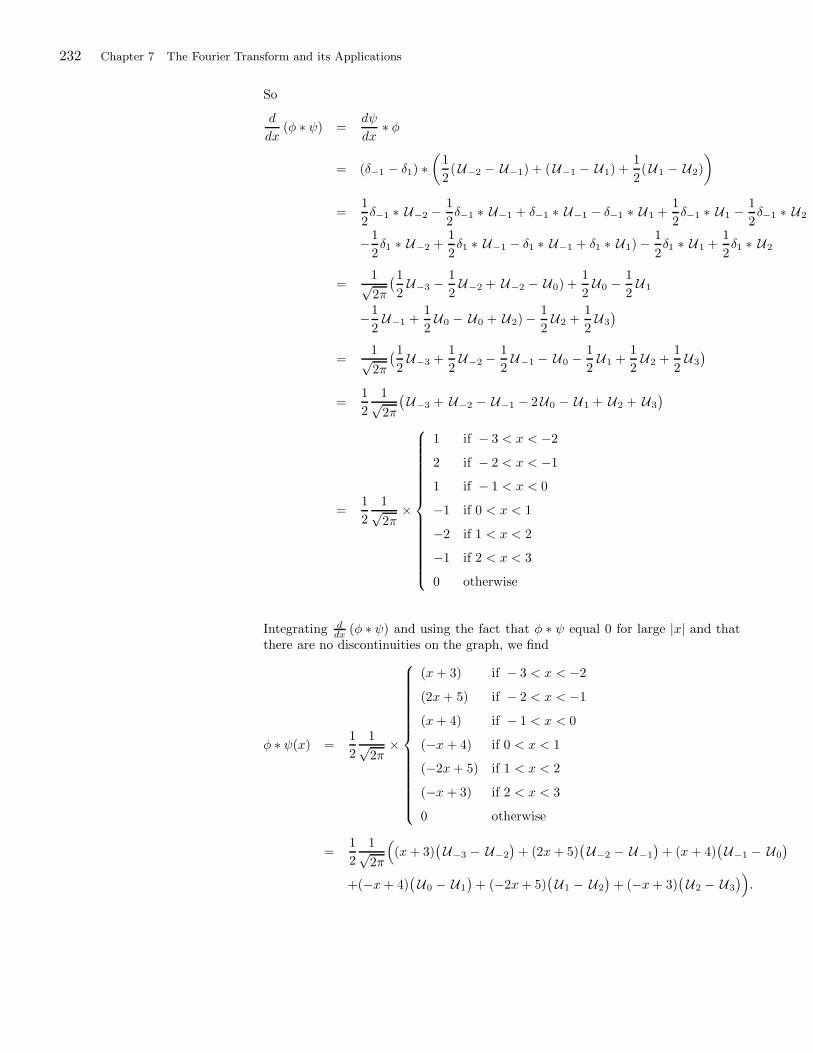
232 Chapter 7 The Fourier Transform and its Applications
So
d
dx(φ ∗ ψ) =
dψ
dx∗ φ
= (δ−1 − δ1) ∗(
1
2(U−2 − U−1) + (U−1 − U1) +
1
2(U 1 − U2)
)
=1
2δ−1 ∗ U−2 −
1
2δ−1 ∗ U−1 + δ−1 ∗ U−1 − δ−1 ∗ U 1 +
1
2δ−1 ∗ U1 −
1
2δ−1 ∗ U2
−1
2δ1 ∗ U−2 +
1
2δ1 ∗ U−1 − δ1 ∗ U−1 + δ1 ∗ U1) −
1
2δ1 ∗ U 1 +
1
2δ1 ∗ U2
=1√2π
(12U−3 −
1
2U−2 + U−2 − U0) +
1
2U0 −
1
2U 1
−1
2U−1 +
1
2U0 − U0 + U2) −
1
2U2 +
1
2U3
)
=1√2π
(12U−3 +
1
2U−2 −
1
2U−1 − U0 −
1
2U1 +
1
2U2 +
1
2U3
)
=1
2
1√2π
(U−3 + U−2 − U−1 − 2U0 − U 1 + U2 + U3
)
=1
2
1√2π
×
1 if − 3 < x < −2
2 if − 2 < x < −1
1 if − 1 < x < 0
−1 if 0 < x < 1
−2 if 1 < x < 2
−1 if 2 < x < 3
0 otherwise
Integrating ddx (φ ∗ ψ) and using the fact that φ ∗ ψ equal 0 for large |x| and that
there are no discontinuities on the graph, we find
φ ∗ ψ(x) =1
2
1√2π
×
(x+ 3) if − 3 < x < −2
(2x+ 5) if − 2 < x < −1
(x+ 4) if − 1 < x < 0
(−x + 4) if 0 < x < 1
(−2x+ 5) if 1 < x < 2
(−x + 3) if 2 < x < 3
0 otherwise
=1
2
1√2π
((x+ 3)
(U−3 − U−2
)+ (2x+ 5)
(U−2 − U−1
)+ (x+ 4)
(U−1 − U0
)
+(−x+ 4)(U0 − U1
)+ (−2x+ 5)
(U1 − U2
)+ (−x+ 3)
(U2 − U3
)).
Section 7.9 The Nonhomogeneous Heat Equation 233
Solutions to Exercises 7.9
1. Proceed as in Example 1 with c = 1/2. Equation (3) becomes in this case
u(x, t) =2√2te−x2/t ∗ δ1(x)
=1√πte−(x−1)2/t,
since the effect of convolution by δ1 is to shift the function by 1 unit to the rightand multiply by 1√
2π.
3. We use the superposition principle (see the discussion preceeding Example 4).If φ is the solution of ut = 1
4uxx + δ0, u(x, 0) = 0 and ψ is the solution of ut =14uxx+δ1, u(x, 0) = 0, then φ+ψ is the solution of ut = 1
4uxx+δ0 +δ1, u(x, 0) = 0.
Applying Examples 2 and 4, we find
φ(x, t) =2√t√πe−x2/t − 2|x|√
πΓ
(1
2,x2
t
)
and
ψ =2√t√πe−(x−1)2/t − 2|x− 1|√
πΓ
(1
2,
(x− 1)2
t
).
5. We use the superposition principle (see the discussion preceeding Example 4). Ifφ is the solution of ut = 1
4uxx + δ0, u(x, 0) = 0 and ψ is the solution of ut = 14uxx,
u(x, 0) = U0(x), then you can check that φ+ ψ is the solution of ut = 14uxx + δ0,
u(x, 0) = U0(x). By Examples 1,
φ(x, t) =2√t√πe−x2/t − 2|x|√
πΓ
(1
2,x2
t
)
and by Exercise 20, Section 7.4,
ψ(x, t) =1
2erf
(x√t
).
7. See the end of Section 7.4 for related topics.
9. Apply Theorem 2 with c = 1 and f(x, t) = cos ax; then
u(x, t) =
∫ t
0
∫ ∞
−∞
1
2√π(t− s)
e−(x−y)2/(4(t−s)) cos(ay) dyds
=
∫ t
0
1√2π
∫ ∞
−∞
1√2(t− s)
e−y2/(4(t−s)) cos(a(x− y)) dyds
(Change variables x− y ↔ y)
= cos(ax)
∫ t
0
1√2π
∫ ∞
−∞
1√2(t− s)
e−y2/(4(t−s)) cos(ay) dyds
(Integral of odd function is 0.
= cos(ax)
∫ t
0
e−a2(t−s)ds (Fourier transform of a Guaussian.)
=1
a2cos(ax)
(1 − e−a2t
).
11. Write the Fourier series of f(x) in the form
f(x) = a0 +
∞∑
n=1
(an cosnx+ bn sinnx
).
234 Chapter 7 The Fourier Transform and its Applications
It is not hard to derive the solution of
ut = uxx + a0, u(x, 0) = 0,
as u0(x, t) = a0t. Now use superposition and the results of Exercises 9 and 10 toconclude that the solution of
ut = uxx + a0 +
∞∑
n=1
(an cos nx+ bn sinnx
)
is
u(x, t) = a0t+
∞∑
n=1
1 − e−n2t
n2(an cosnx+ bn sinnx) .
Section 7.10 Duhamel’s Principle 235
Solutions to Exercises 7.10
1. Apply Proposition 1 with f(x, s) = e−(x+s)2 , then
dU
dx= f(x, x) +
∫ x
0
∂
∂xf(x, s) ds
= e−4x2 −∫ x
0
2(x+ s)e−(x+s)2 ds
= e−4x2 −∫ 2x
x
2ve−v2
dv ((v = x+ s)
= e−4x2
+ e−v2∣∣∣2x
x= 2e−4x2 − e−x2
.
3. Use the product rule for differentiation and Proposition 1 and get
d
dx
(x2
∫ x
0
f(x, s) ds
)= 2x
∫ x
0
f(x, s) ds+ x2 d
dx
∫ x
0
f(x, s) ds
= 2x
∫ x
0
f(x, s) ds+ x2
(f(x, x) +
∫ x
0
∂
∂xf(x, s) ds
).
5. Following Theorem 1, we first solve φt = φxx, φ(x, 0, s) = e−sx2, where s > 0is fixed. The solution is φ(x, t, s) = e−s(2t + x2) (see the solution of Exercise 5,Section 7.4). The the desired solution is given by
u(x, t) =
∫ t
0
φ(x, t− s, s)ds
=
∫ t
0
e−s(2(t− s) + x2)ds
= −2te−s + 2se−s + 2e−s − x2e−s∣∣∣t
0
= −2 + 2t+ x2 + e−t(2 − x2).
7. Following Theorem 2, we first solve φtt = φxx, φ(x, 0, s) = 0, φt(x, 0, s) = cos xwhere s > 0 is fixed. By d’Alembert’s method, the solution is
φ(x, t, s) =1
2
∫ x+t
x−t
cos y dy =1
2
[sin(x+ t) − sin(x− t)
].
The the desired solution is given by
u(x, t) =
∫ t
0
φ(x, t− s, s)ds
=1
2
∫ t
0
[sin(x+ t − s) − sin(x− t+ s)
]ds
=1
2
[cos(x+ t− s) + cos(x− t + s)
]∣∣∣t
0
=1
2
[2 cosx− cos(x+ t) − cos(x− t)
].
236 Chapter 7 The Fourier Transform and its Applications
9. Following Theorem 2, we first solve φtt = φxx, φ(x, 0, s) = 0, φt(x, 0, s) =cos(s+ x) where s > 0 is fixed. By d’Alembert’s method, the solution is
φ(x, t, s) =1
2
∫ x+t
x−t
cos(s+ y) dy =1
2
[sin(s+ x+ t) − sin(s+ x− t)
].
The the desired solution is given by
u(x, t) =
∫ t
0
φ(x, t− s, s)ds
=1
2
∫ t
0
[sin(x+ t) − sin(x− t + 2s)
]ds
=1
2
[s sin(x+ t) +
1
2cos(x− t+ 2s)
]∣∣∣t
0
=1
2
[t sin(x+ t) +
1
2cos(x+ t) − 1
2cos(x− t)
].
11. We use superposition and start by solving φtt = φxx, φ(x, 0, s) = 0, φt(x, 0, s) =x cos s where s > 0 is fixed. By d’Alembert’s method, the solution is
φ(x, t, s) =1
2
∫ x+t
x−t
y cos s dy =cos s
4
[(x+ t)2 − (x− t)2
]= xt cos s.
By Theorem 2, the solution of φtt = φxx +x cos t, φ(x, 0) = 0, φt(x, 0) = 0 is givenby
φ(x, t) =
∫ t
0
φ(x, t− s, s)ds
=
∫ t
0
x
u︷ ︸︸ ︷(t− s)
dv︷ ︸︸ ︷cos s ds (Integrate by parts.)
= x
[(t − s) sin s
∣∣∣t
0+
∫ t
0
sin s ds
]
= x(1 − cos t).
Next, we solve ψtt = ψxx, ψ(x, 0) = 0, ψt(x, 0) = x. D’Alembert’s method impliesthat
ψ(x, t) =1
2
∫ x+t
x−t
y dy =1
4y2∣∣∣x+t
x−t= xt.
Thus the solution of the desired problem is
u(x, t) = φ(x, t) + ψ(x, t) = x(1 − cos t) + xt = x(1 + t− cos t).
The validity of this solution can be checked by plugging it back into the equationand the initial conditions.
13. start by solving φtt = φxx, φ(x, 0, s) = 0, φt(x, 0, s) = δ0(x) where s > 0 isfixed. By d’Alembert’s method, the solution is
φ(x, t, s) =1
2
∫ x+t
x−t
δ0(y) dy =1
2
[U0(x+ t) − U0(x− t)
].
By Theorem 2, the solution of utt = uxx + δ0(x), u(x, 0) = 0, φt(x, 0) = 0 is given
Section 7.10 Duhamel’s Principle 237
by
φ(x, t) =
∫ t
0
φ(x, t − s, s)ds
=1
2
∫ t
0
[U0(x+ t− s) − U 0(x− t+ s)
]ds
=1
2
[− τ (x+ t − s) − τ (x− t+ s)
]∣∣∣t
0
= −τ (x) +1
2
[τ (x+ t) + τ (x− t)
],
where τ = τ0 is the antiderivative of U0 described in Example 2, Section 7.8,
238 Chapter 8 The Laplace and Hankel Transforms with Applications
Solutions to Exercises 8.1
1. |11 cos3t| ≤ 11, so (2) holds if you take M = 11 and a any positive number, saya = 1. Note that (2) also holds with a = 0.
3. The function 5e3t is already in the form that appears in (2). Take M = 5 anda = 3.
5. | sinh3t| = |(e3t − e−3t)/2| ≤ (e3t + e3t)/2 = e3t. So (2) holds with M = 1 anda = 3.
7. Using linearity of the Laplace transform and results from Examples 1 and 2, wehave
L(2t+ 3)(s) = 2L(t) + 3L(1)
=2
s2+
3
s
9. Using linearity of the Laplace transform and results from Examples 1 and 2, wehave
L(√t+
1√t)(s) = L(t1/2) + L(t−1/2)
=Γ(3/2)
s3/2+
Γ(1/2)
s1/2
Now Γ(1/2) =√π, so Γ(3/2) = (1/2)Γ(1/2) =
√π/2. Thus
L(√t+
1√t)(s) =
√π
2s3/2+
√π
s.
11. Apply Theorem 5:
L(t2 e3t)(s) = L(t2)(s− 3) =2
(s− 3)3
13. Use Example 3 and Theorem 4:
L(t sin 4t)(s) = − d
dsL(sin(4t)) = − d
ds
4
s2 + 42
=8s
(s2 + 42)2
15. We have sin2 t = 1−cos2t2 , so
L(sin2 t)(s) = L(1/2) − 1/2L(cos(2t) =1
2s− s
2(s2 + 4)
17. We have
L(e2t sin 3t)(s) = L(sin 3t)(s− 2) =3
(s− 2)2 + 32
3
(s− 2)2 + 9
19. We have
L(te−t sin t)(s) = − d
dsL(e−t sin t)(s) = − d
dsL(sin t)(s+ 1)
= − d
ds
1
(s+ 1)2 + 1
=2(s+ 1)
((s+ 1)2 + 1)2
Section 8.1 The Laplace Transform 239
21. We have
L((t+ 2)2 cos t)(s) = L((t2 + 4t+ 4) cos t)(s)
= L(t2 cos t)(s) + 4L(t cos t)(s) + 4L(cos t)(s)
=d2
ds2L(cos t)(s) − 4
d
ds[L(cos t)(s)] + 4L(cos t)(s)
=d2
ds2s
s2 + 1− 4
d
ds
[s
s2 + 1
]+
4s
s2 + 1
=d
ds
−s2 + 1
(s2 + 1)2− 4
−s2 + 1
(s2 + 1)2+
4s
s2 + 1
=2s(s2 − 3)
(s2 + 1)3+ 4
s2 − 1
(s2 + 1)2+
4s
s2 + 1
23. We have
L(eαt sinβt)(s) = L(sinβt)(s − α) =β
(s− α)2 + β2
24. We have
L(eαt cosβt)(s) = L(cos βt)(s− α) =s− α
(s− α)2 + β2
25. Since
L(t) =1
s2;
then
L−1
(1
s2
)= t
27. Write
F (s) =4
3s2 + 1=
4
3
1
s2 +(
1√3
)2=
4√
3
3
1/√
3
s2 +(
1√3
)2
=4√3L(
sint√3
);
and so
f(t) =4√3
sint√3.
29. Using
L(eattn
)=
n!
(s− a)n+1,
L(eattn
n!
)=
1
(s− a)n+1,
L(eat cos bt
)=
s− a
(s− a)2 + b2,
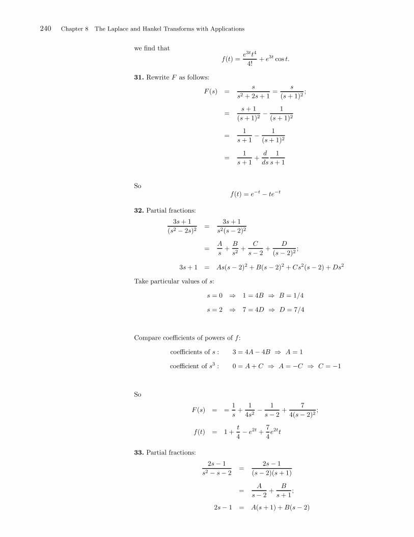
240 Chapter 8 The Laplace and Hankel Transforms with Applications
we find that
f(t) =e3tt4
4!+ e3t cos t.
31. Rewrite F as follows:
F (s) =s
s2 + 2s+ 1=
s
(s+ 1)2;
=s+ 1
(s+ 1)2− 1
(s+ 1)2
=1
s+ 1− 1
(s+ 1)2
=1
s+ 1+
d
ds
1
s+ 1
Sof(t) = e−t − te−t
32. Partial fractions:
3s+ 1
(s2 − 2s)2=
3s+ 1
s2(s− 2)2
=A
s+B
s2+
C
s− 2+
D
(s− 2)2;
3s+ 1 = As(s− 2)2 +B(s − 2)2 +Cs2(s− 2) +Ds2
Take particular values of s:
s = 0 ⇒ 1 = 4B ⇒ B = 1/4
s = 2 ⇒ 7 = 4D ⇒ D = 7/4
Compare coefficients of powers of f :
coefficients of s : 3 = 4A− 4B ⇒ A = 1
coefficient of s3 : 0 = A+ C ⇒ A = −C ⇒ C = −1
So
F (s) = =1
s+
1
4s2− 1
s− 2+
7
4(s− 2)2;
f(t) = 1 +t
4− e2t +
7
4e2tt
33. Partial fractions:
2s− 1
s2 − s− 2=
2s− 1
(s− 2)(s+ 1)
=A
s− 2+
B
s+ 1;
2s− 1 = A(s+ 1) + B(s− 2)
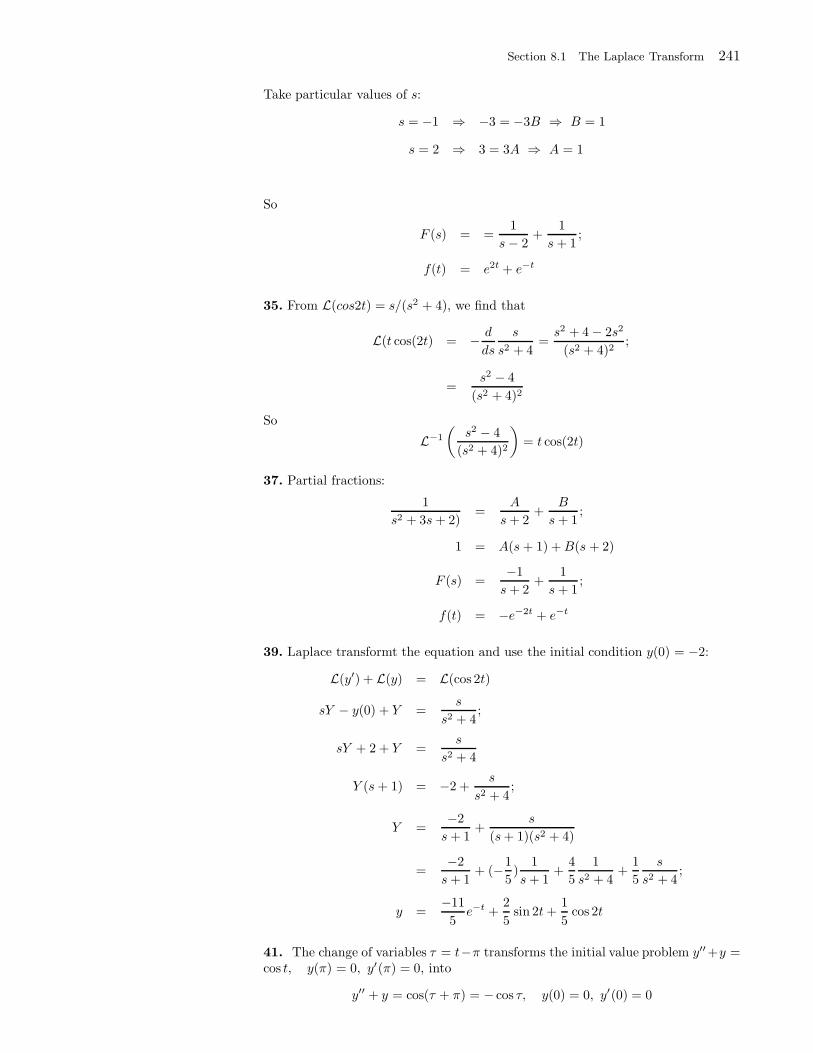
Section 8.1 The Laplace Transform 241
Take particular values of s:
s = −1 ⇒ −3 = −3B ⇒ B = 1
s = 2 ⇒ 3 = 3A ⇒ A = 1
So
F (s) = =1
s− 2+
1
s+ 1;
f(t) = e2t + e−t
35. From L(cos2t) = s/(s2 + 4), we find that
L(t cos(2t) = − d
ds
s
s2 + 4=s2 + 4 − 2s2
(s2 + 4)2;
=s2 − 4
(s2 + 4)2
So
L−1
(s2 − 4
(s2 + 4)2
)= t cos(2t)
37. Partial fractions:
1
s2 + 3s+ 2)=
A
s+ 2+
B
s+ 1;
1 = A(s+ 1) +B(s + 2)
F (s) =−1
s+ 2+
1
s+ 1;
f(t) = −e−2t + e−t
39. Laplace transformt the equation and use the initial condition y(0) = −2:
L(y′) + L(y) = L(cos 2t)
sY − y(0) + Y =s
s2 + 4;
sY + 2 + Y =s
s2 + 4
Y (s+ 1) = −2 +s
s2 + 4;
Y =−2
s+ 1+
s
(s+ 1)(s2 + 4)
=−2
s+ 1+ (−1
5)
1
s+ 1+
4
5
1
s2 + 4+
1
5
s
s2 + 4;
y =−11
5e−t +
2
5sin 2t+
1
5cos 2t
41. The change of variables τ = t−π transforms the initial value problem y′′+y =cos t, y(π) = 0, y′(π) = 0, into
y′′ + y = cos(τ + π) = − cos τ, y(0) = 0, y′(0) = 0
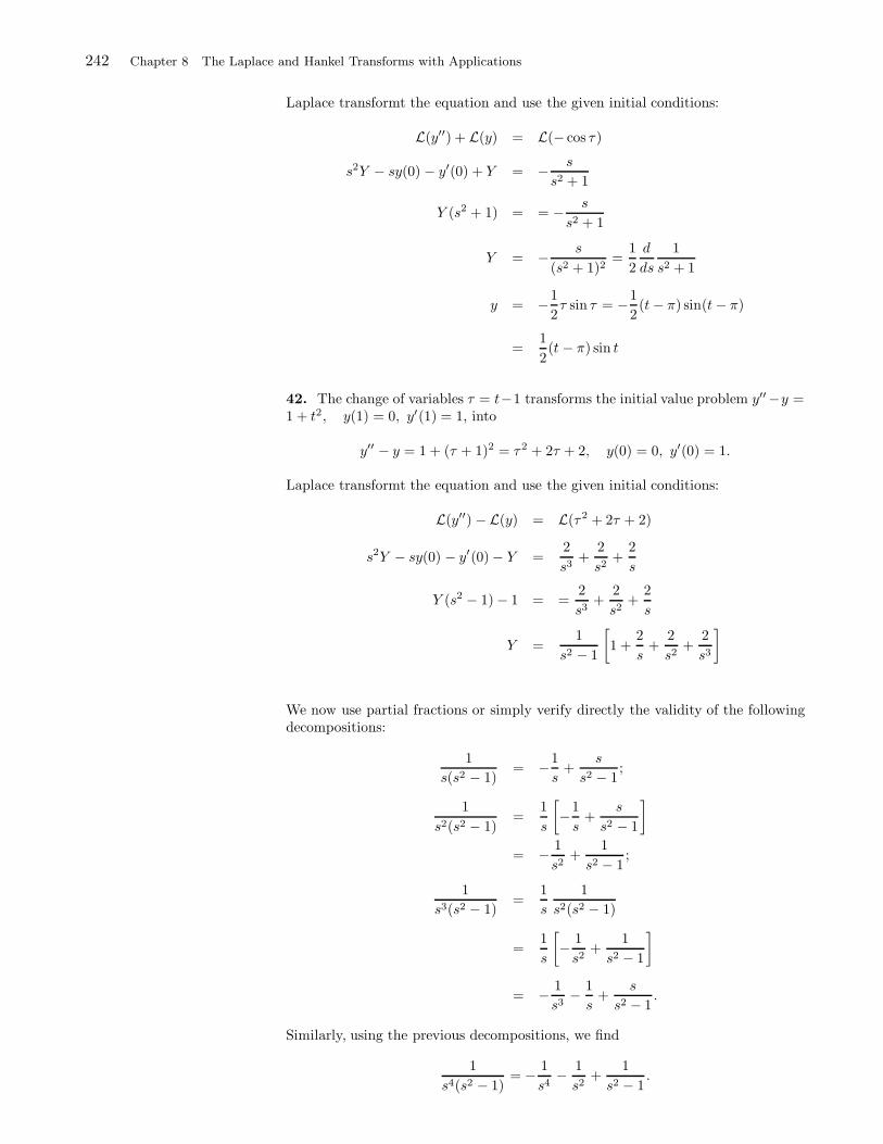
242 Chapter 8 The Laplace and Hankel Transforms with Applications
Laplace transformt the equation and use the given initial conditions:
L(y′′) + L(y) = L(− cos τ )
s2Y − sy(0) − y′(0) + Y = − s
s2 + 1
Y (s2 + 1) = = − s
s2 + 1
Y = − s
(s2 + 1)2=
1
2
d
ds
1
s2 + 1
y = −1
2τ sin τ = −1
2(t− π) sin(t− π)
=1
2(t − π) sin t
42. The change of variables τ = t−1 transforms the initial value problem y′′−y =1 + t2, y(1) = 0, y′(1) = 1, into
y′′ − y = 1 + (τ + 1)2 = τ2 + 2τ + 2, y(0) = 0, y′(0) = 1.
Laplace transformt the equation and use the given initial conditions:
L(y′′) −L(y) = L(τ2 + 2τ + 2)
s2Y − sy(0) − y′(0) − Y =2
s3+
2
s2+
2
s
Y (s2 − 1) − 1 = =2
s3+
2
s2+
2
s
Y =1
s2 − 1
[1 +
2
s+
2
s2+
2
s3
]
We now use partial fractions or simply verify directly the validity of the followingdecompositions:
1
s(s2 − 1)= −1
s+
s
s2 − 1;
1
s2(s2 − 1)=
1
s
[−1
s+
s
s2 − 1
]
= − 1
s2+
1
s2 − 1;
1
s3(s2 − 1)=
1
s
1
s2(s2 − 1)
=1
s
[− 1
s2+
1
s2 − 1
]
= − 1
s3− 1
s+
s
s2 − 1.
Similarly, using the previous decompositions, we find
1
s4(s2 − 1)= − 1
s4− 1
s2+
1
s2 − 1.
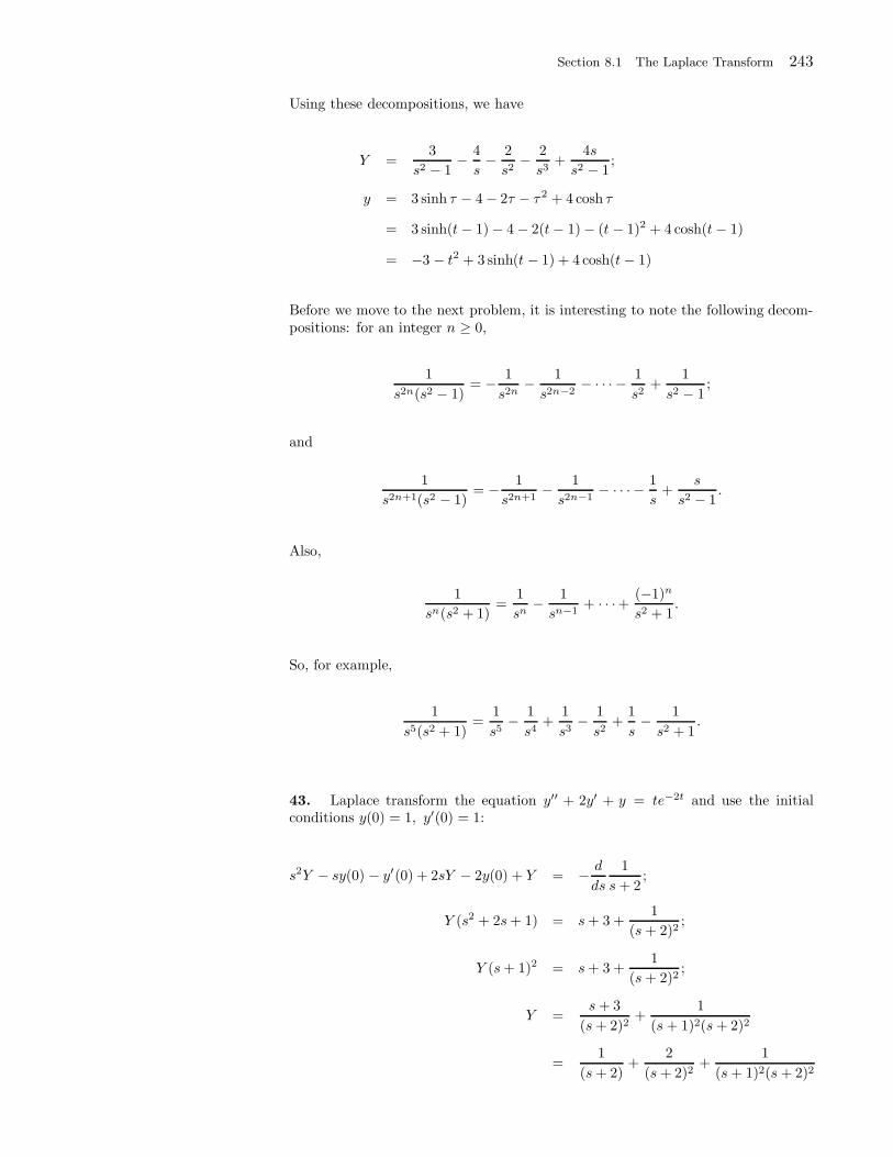
Section 8.1 The Laplace Transform 243
Using these decompositions, we have
Y =3
s2 − 1− 4
s− 2
s2− 2
s3+
4s
s2 − 1;
y = 3 sinh τ − 4 − 2τ − τ2 + 4 cosh τ
= 3 sinh(t− 1) − 4 − 2(t− 1) − (t − 1)2 + 4 cosh(t− 1)
= −3 − t2 + 3 sinh(t − 1) + 4 cosh(t− 1)
Before we move to the next problem, it is interesting to note the following decom-positions: for an integer n ≥ 0,
1
s2n(s2 − 1)= − 1
s2n− 1
s2n−2− · · · − 1
s2+
1
s2 − 1;
and
1
s2n+1(s2 − 1)= − 1
s2n+1− 1
s2n−1− · · · − 1
s+
s
s2 − 1.
Also,
1
sn(s2 + 1)=
1
sn− 1
sn−1+ · · ·+ (−1)n
s2 + 1.
So, for example,
1
s5(s2 + 1)=
1
s5− 1
s4+
1
s3− 1
s2+
1
s− 1
s2 + 1.
43. Laplace transform the equation y′′ + 2y′ + y = te−2t and use the initialconditions y(0) = 1, y′(0) = 1:
s2Y − sy(0) − y′(0) + 2sY − 2y(0) + Y = − d
ds
1
s+ 2;
Y (s2 + 2s+ 1) = s+ 3 +1
(s+ 2)2;
Y (s+ 1)2 = s+ 3 +1
(s+ 2)2;
Y =s+ 3
(s+ 2)2+
1
(s+ 1)2(s+ 2)2
=1
(s+ 2)+
2
(s+ 2)2+
1
(s+ 1)2(s+ 2)2
244 Chapter 8 The Laplace and Hankel Transforms with Applications
We now find the partial frctions decomposition of the last term on the right. Write
1
(s+ 1)2(s+ 2)2=
A
s+ 1+ +
B
(s+ 1)2+
C
s+ 2+
D
(s+ 2)2;
1 = A(s+ 1)(s+ 2)2 +B(s + 2)2 +C(s+ 1)2(s+ 2) +D(s+ 1)2;
s = −1 ⇒ B = 1
s = −2 ⇒ D = 1;
s = 0 ⇒ 1 = 4A+ 4 + 2C + 1 ⇒ A+C = 0
compare coefficiets of s3 ⇒ 0 = A +C;
⇒ A = −2, C = 2;
1
(s+ 1)2(s+ 2)2=
−2
s+ 1+
1
(s+ 1)2+
2
s+ 2+
1
(s+ 2)2
Y =−1
s+ 1+
3
(s+ 1)2+
2
s+ 2+
1
(s+ 2)2
y = −e−t + 3te−t + 2e−2t + te−2t.
45. Laplace transform the equation y′′ − y′ − 6y = et cos t and use the initialconditions y(0) = 0, y′(0) = 1:
s2Y − sy(0) − y′(0) − sY + y(0) − 6Y =s− 1
(s− 1)2 + 1;
Y (s2 − s− 6) = 1 +s− 1
(s− 1)2 + 1;
So
Y =1
(s− 3)(s+ 2)+
1
(s− 3)(s+ 2)
s− 1
(s− 1)2 + 1;
Y =−1
5(s+ 2)+
1
5(s− 3)+
1
(s− 3)(s+ 2)
s− 1
s2 − 2s+ 2
=−1
5(s+ 2)+
1
5(s− 3)+
1
(s+ 2)(s2 − 2s+ 2)+
2
(s− 3)(s+ 2)(s2 − 2s+ 2)
We now find the partial frctions decomposition of the last term on the right. Write
1
(s+ 2)(s2 − 2s+ 2)=
A
s+ 2+ +
Bs+ C
s2 − 2s+ 2;
1 = A(s2 − 2s+ 2) + (Bs+ C)(s+ 2);
s = −2 ⇒ 1 = 10A ⇒ A = 1/10
constant term ⇒ 1 =1
5+ 2C ⇒ C = 2/5;
coefficient of s2 ⇒ 0 =1
10+B ⇒ B = −1/10;
1
(s+ 2)(s2 − 2s+ 2)=
1
10(s+ 2)+ +
−s+ 4
10(s2 − 2s+ 2)
= Y1.
Section 8.1 The Laplace Transform 245
Also
2
(s− 3)(s+ 2)(s2 − 2s+ 2)=
A
s− 3+ +
B
s+ 2+
CS +D
(s− 3)(s+ 2)(s2 − 2s+ 2);
2 = A(s+ 2)(s2 − 2s+ 2) +B(s − 3)(s2 − 2s+ 2)
+(CS +D)(s − 3)(s+ 2);
s = −2 ⇒ B = −1/25
s = −3 ⇒ A = 2/25
constant term ⇒ 2 =8
25+
6
25− 6D ⇒ D = −6/25;
coefficient of s3 ⇒ C = −1/25;
2
(s− 3)(s+ 2)(s2 − 2s+ 2)=
2
25(s− 3)− 1
25(s+ 2)+
−s− 6
25(s2 − 2s+ 2)
= Y2;
Now
Y =−1
5(s+ 2)+
1
5(s− 3)+ Y1 + Y2
y = − 7
50e−2t +
7
25e3t − 7
50et cos t+
1
50et sin t.
47. The function y = sinat is the unique solution of the initial value problem
y′′ + a2y = 0 y(0) = 0, y′(0) = a.
Taking the Laplace transform of the initial value problem, we find
s2Y − sy(0) − y′(0) + a2Y = 0 ⇒ Y (s2 + a2) = a
⇒ Y =a
s2 + a2
⇒ L(sin at) =a
s2 + a2
246 Chapter 8 The Laplace and Hankel Transforms with Applications
Solutions to Exercises 8.2
1. To compute the Laplace transform of f(t) = U0(t − 1) − t+ 1, use
L [U0(t− a)] (s) =e−as
s;
so
L [U0(t− 1) − t+ 1] (s) = L [U0(t− 1)]− L [t] + L [1]
=e−s
s− 1
s2+
1
s.
3. To compute the Laplace transform of f(t) = e2tU0(t − 2), we first prepare thefunction to be in a form suitable for the application of Theorem 1. Write
e2tU0(t− 2) = e4e2(t−2)U0(t − 2);
L[e4e2(t−2)U0(t− 2)
](s) = e4L
[e2(t−2)U0(t − 2)
](s)
= e4e−2sL[e2t]
= e4e−2s 1
s− 2=e−2(s−2)
s− 2.
Alternatively, we can use Theorem 5 of the previous section and compute theLaplace transform as follows:
L[e2tU0(t− 2)
](s) = L [U0(t− 2)] (s− 2)
= L [U0(t− 2)] (s− 2)
=e−2(s−2)
s− 2,
because
L [U0(t − 2)] (s) =e−2s
s.
5. Use the identity sin t = − sin(t − π). Then
L [sin tU0(t − π)] (s) = −L [sin(t − π)U0(t− π)] (s)
= −e−πsL [sin t] (s) =−e−πs
s2 + 1.
7. y = U0(t) − U0(t− 2), Y = 1s − e−2s
s
9.
y = 2 (U0(t− 2) − U0(t− 3)) ;
Y = 2e−2s
s− e−3s
s
Section 8.2 Further Properties of The Laplace Transform 247
11. This is the translate of the function in Exercise 10. You can write its formulaby translating the formula in Exercise 10:
y = (t − 1)U0(t− 1) − (t− 2)U0(t − 2) − U0(t− 2);
Y =e−s
s2− e−2s
s2− e−2s
s
13.
y = (U0(t− 1) − U0(t− 4)) + (t− 5) (U0(t− 4) − U 0(t − 5))
= U0(t− 1) − U0(t− 4) + (t − 5)U0(t− 5) + (t − 4)U0(t− 4) − U0(t− 4);
Y =e−s
s− 2
e−4s
s+e−4s
s2− e−5s
s2
The following is a variation on Exercise 13.
13 bis. Find the Laplace transform of the function in the picture
y = (U0(t− 1) − U0(t− 4)) + (5 − t) (U0(t− 4) − U 0(t − 5))
= U0(t− 1) − U0(t− 4) + (t − 5)U0(t− 5) − (t − 5)U0(t− 4)
= U0(t− 1) − U0(t− 4) + (t − 5)U0(t− 5) − (t − 4)U0(t− 4) + U0(t− 4);
Y =e−s
s− e−4s
s+e−5s
s2− e−4s
s2+e−4s
s
=e−s
s+
1
s2(e−5s − e−4s
)
248 Chapter 8 The Laplace and Hankel Transforms with Applications
15. Let y(t) = t, then Y (s) = 1s2 ; so if f(t) = (t− 1)U0(t − 1), then F (s) = e−s
s2
17. Let y(t) = sin t, then Y (s) = 1s2+1
; so if
f(t) = U0(t − 1) sin(t− 1),
then F (s) =e−s
s2 + 1.
19. Let y(t) = cos t, then Y (s) = ss2+1
. To shift the transform by 3, we multiply
the function by e3t. So, if
f(t) = e3t cos t,
then F (s) =s− 3
1 + (s− 3)2.
20. Let y(t) = sinh tt, then Y (s) = 1s2−1
. So, if
f(t) = U0(t− 3) sinh(t − 3),
then F (s) =e−3s
(s− 1)(s+ 1).
21. Let y(t) =√t, then Y (s) = Γ(3/2)
s3/2 , where Γ(3/2) = 12Γ(1/2) = π
2 . If
φ(t) =2
π
√t⇒ Φ(s) =
1
s3/2;
and so if
f(t) =2
π
√t− 1U0(t− 1) then F (s) =
e−s
s3/2.
23. We will compute 1 ∗ t in two different ways. First method: We have
1L−→ 1
s;
tL−→ 1
s2;
1 ∗ t L−→ 1
s· 1
s2=
1
s3
1
s3L−1
−→ 1
2t2 = 1 ∗ t.
Alternatively,
1 ∗ t =
∫ t
0
τ dτ =1
2τ2∣∣∣t
0=
1
2t2.
25. We will compute t ∗ t in two different ways. First method: We have
tL−→ 1
s2;
tL−→ 1
s2;
t ∗ t L−→ 1
s2· 1
s2=
1
s4
1
s4L−1
−→ t3
6= t ∗ t.
Section 8.2 Further Properties of The Laplace Transform 249
Alternatively,
t ∗ t =
∫ t
0
(t− τ )τ dτ
= t1
2τ2 − 1
3τ3∣∣∣t
0=
1
2t3 − 1
3t3 =
1
6t3.
27. We will compute sin t ∗ sin t in two different ways. First method: We have
sin tL−→ 1
s2 + 1;
sin tL−→ 1
s2 + 1;
sin t ∗ sin tL−→ 1
s2 + 1· 1
s2 + 1=
1
2
[1
s2 + 1+
d
ds
s
s2 + 1
]
1
2
[1
s2 + 1+
d
ds
s
s2 + 1
]L−1
−→ 1
2[sin t− t cos t] = sin t ∗ sin t.
Alternatively,
sin t ∗ sin t =
∫ t
0
sin(t− τ ) sin τ dτ
=1
2
∫ t
0
(cos(t− τ − τ ) − cos(t− τ + τ )
)dτ
=1
2
∫ t
0
(cos(t− 2τ ) − cos t
)dτ
=1
2
(− 1
2sin(t− 2τ ) − (cos t)τ
)dτ∣∣∣t
0
=1
2(sin t− t cos t).
29. We have F (s) = 1s(s2+1) = 1
s · 1s2+1 , and
1
s
L−1
−→ 1;
1
s2 + 1
L−1
−→ sin t.
So
f(t) = 1 ∗ sin t =
∫ t
0
sin τ dτ = 1 − cos t.
31. We have F (s) = 1(s2+1)(s2+1) = 1
s2+1 · 1s2+1 . So So
f(t) = sin t ∗ sin t =1
2
(sin t− t cos t
)(by Exercise 27).
33. Passing the equations y′′ + y = δ0(t − 1), y(0) = 0, y′(0) = 0, through theLaplace transform, we get:
s2Y − sy(0) − y′(0) + Y = e−s
(s2 + 1)Y = e−s
Y =e−s
s2 + 1.
250 Chapter 8 The Laplace and Hankel Transforms with Applications
Thus the solution is
y = L−1
(e−s
s2 + 1
).
To compute this inverse transform, we observe
sin tL−→ 1
s2 + 1;
U0(t − 1) sin(t− 1)L−→ e−s
s2 + 1;
so y = U0(t− 1) sin(t − 1).
35. Take the Laplace transform on both sides of y′′ + 2y′ + y = 3δ0(t− 2) and usethe initial conditions y(0) = 1, y′(0) = 0, and you will get
L (y′′ + 2y′ + y) = L (3δ0(t − 2))
L (y′′) + 2L (y′) + L (y) = 3L (δ0(t − 2)) ;
s2Y − sy(0) − y′(0) + 2(sY − y(0)) + Y = 3e−2s
s2Y − s+ 2(sY − 1) + Y = 3e−2s
Y
(s+1)2
︷ ︸︸ ︷(s2 + 2s+ 1) = 3e−2s + s+ 2;
Y =3e−2s
(s+ 1)2+
s
(s+ 1)2+
2
(s+ 1)2.,
where we have used Theorem 3, Sec. 8.1, and Example 7 of Sec. 8.2. Thus thesolution is the inverse Laplace transform of
3e−2s
(s+ 1)2+
s
(s+ 1)2+
2
(s+ 1)2.
You can use the Table of Laplace transforms at the end of the book to verify thefollowing computations:
te−t L−→ 1
(s+ 1)2
U0(t− 2)f(t − 2)L−→ e−2sF (s);
(t − 2)e−(t−2) U 0(t − 2)L−→ e−2s
(s+ 1)2;
3(t− 2)e−(t−2) U 0(t − 2)L−→ 3
e−2s
(s+ 1)2;
f(t) = te−t L−→ 1
(s+ 1)2
f ′(t) = e−t − te−t L−→ sF (s) − f(0) =s
(s+ 1)2.
Section 8.2 Further Properties of The Laplace Transform 251
From this we conclude that
L−1
(2
(s+ 1)2
)= 2te−t;
L−1
(3
e−2s
(s+ 1)2
)= 3(t − 2)e−(t−2) U0(t− 2);
L−1
(s
(s+ 1)2
)= e−t − te−t;
and so
y(t) = e−t−te−t+3(t−2)e−(t−2) U0(t−2)+2te−t = e−t(1 + t+ 3e2(t − 2)U0(t− 2)
).
35 Bis. (This problem has a different initial condition than the original Exercise 35.
Take the Laplace transform on both sides of y′′ + 2y′ + y = 3δ0(t− 2) and usethe initial conditions y(0) = 1, y′(0) = 0, and you will get
L (y′′ + 2y′ + y) = L (3δ0(t − 2))
L (y′′) + 2L (y′) + L (y) = 3L (δ0(t − 2)) ;
s2Y − sy(0) − y′(0) + 2(sY − y(0)) + Y = 3e−2s
s2Y − s− 1 + 2(sY − 1) + Y = 3e−2s
Y︷ ︸︸ ︷(s2 + 2s+ 1) (s+ 1)2 = 3e−2s + s+ 3;
Y =3e−2s
(s+ 1)2+
s
(s+ 1)2+
3
(s+ 1)2.,
where we have used Theorem 3, Sec. 8.1, and Example 7 of Sec. 8.2. Thus thesolution is the inverse Laplace transform of
3e−2s
(s+ 1)2+
s
(s+ 1)2+
3
(s+ 1)2.
You can use the Table of Laplace transforms at the end of the book to verify thefollowing computations:
te−t L−→ 1
(s+ 1)2
U0(t− 2)f(t − 2)L−→ e−2sF (s);
(t − 2)e−(t−2) U 0(t − 2)L−→ e−2s
(s+ 1)2;
3(t− 2)e−(t−2) U 0(t − 2)L−→ 3
e−2s
(s+ 1)2;
f(t) = te−t L−→ 1
(s+ 1)2
f ′(t) = e−t − te−t L−→ sF (s) − f(0) =s
(s+ 1)2.
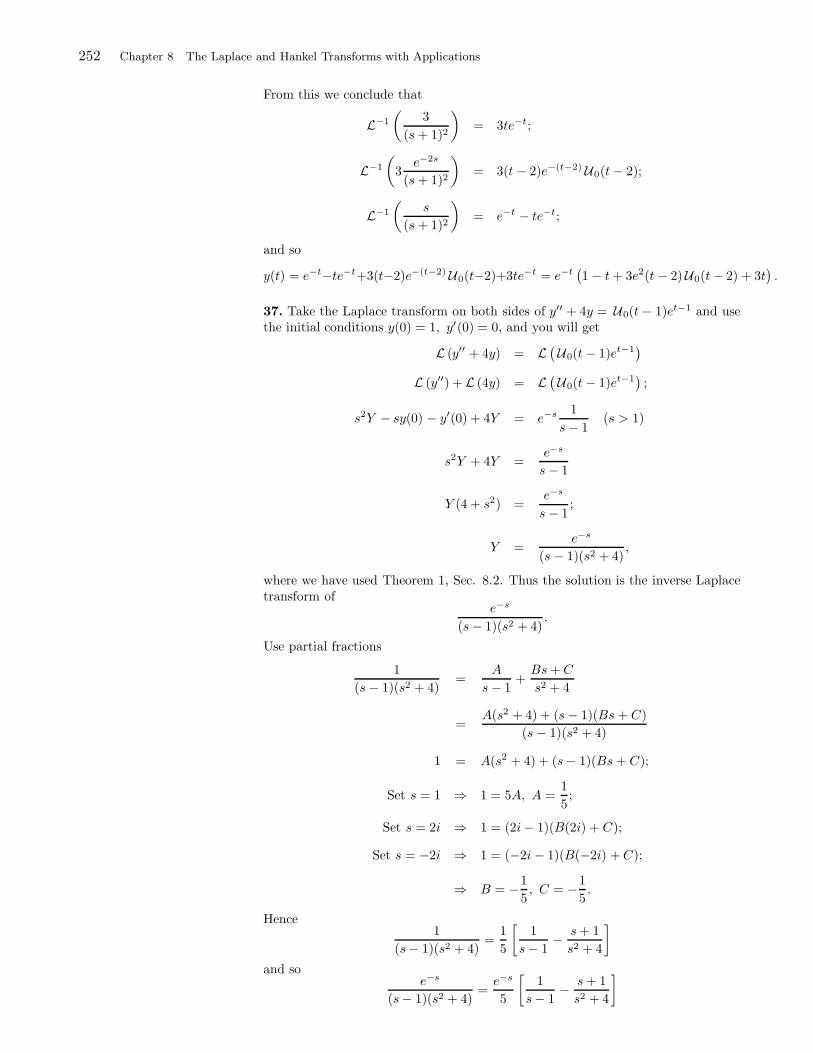
252 Chapter 8 The Laplace and Hankel Transforms with Applications
From this we conclude that
L−1
(3
(s+ 1)2
)= 3te−t;
L−1
(3
e−2s
(s+ 1)2
)= 3(t − 2)e−(t−2) U0(t− 2);
L−1
(s
(s+ 1)2
)= e−t − te−t;
and so
y(t) = e−t−te−t+3(t−2)e−(t−2) U0(t−2)+3te−t = e−t(1 − t+ 3e2(t − 2)U0(t− 2) + 3t
).
37. Take the Laplace transform on both sides of y′′ + 4y = U0(t − 1)et−1 and usethe initial conditions y(0) = 1, y′(0) = 0, and you will get
L (y′′ + 4y) = L(U0(t − 1)et−1
)
L (y′′) + L (4y) = L(U0(t − 1)et−1
);
s2Y − sy(0) − y′(0) + 4Y = e−s 1
s− 1(s > 1)
s2Y + 4Y =e−s
s− 1
Y (4 + s2) =e−s
s− 1;
Y =e−s
(s− 1)(s2 + 4),
where we have used Theorem 1, Sec. 8.2. Thus the solution is the inverse Laplacetransform of
e−s
(s− 1)(s2 + 4).
Use partial fractions
1
(s− 1)(s2 + 4)=
A
s− 1+Bs+C
s2 + 4
=A(s2 + 4) + (s− 1)(Bs+ C)
(s− 1)(s2 + 4)
1 = A(s2 + 4) + (s− 1)(Bs+ C);
Set s = 1 ⇒ 1 = 5A, A =1
5;
Set s = 2i ⇒ 1 = (2i− 1)(B(2i) + C);
Set s = −2i ⇒ 1 = (−2i− 1)(B(−2i) +C);
⇒ B = −1
5, C = −1
5.
Hence1
(s− 1)(s2 + 4)=
1
5
[1
s− 1− s+ 1
s2 + 4
]
and soe−s
(s− 1)(s2 + 4)=e−s
5
[1
s− 1− s+ 1
s2 + 4
]
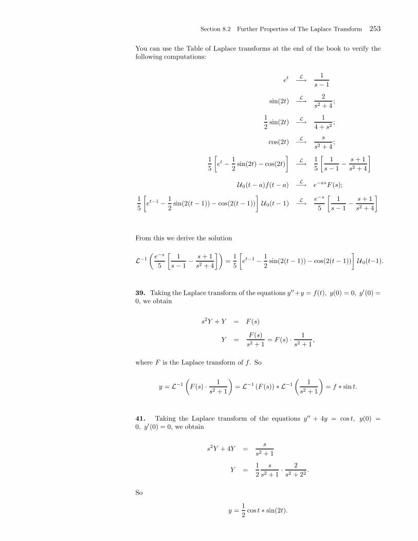
Section 8.2 Further Properties of The Laplace Transform 253
You can use the Table of Laplace transforms at the end of the book to verify thefollowing computations:
et L−→ 1
s− 1
sin(2t)L−→ 2
s2 + 4;
1
2sin(2t)
L−→ 1
4 + s2;
cos(2t)L−→ s
s2 + 4;
1
5
[et − 1
2sin(2t) − cos(2t)
]L−→ 1
5
[1
s− 1− s+ 1
s2 + 4
]
U0(t− a)f(t − a)L−→ e−asF (s);
1
5
[et−1 − 1
2sin(2(t − 1)) − cos(2(t− 1))
]U0(t− 1)
L−→ e−s
5
[1
s− 1− s+ 1
s2 + 4
]
From this we derive the solution
L−1
(e−s
5
[1
s− 1− s+ 1
s2 + 4
])=
1
5
[et−1 − 1
2sin(2(t− 1)) − cos(2(t− 1))
]U 0(t−1).
39. Taking the Laplace transform of the equations y′′+y = f(t), y(0) = 0, y′(0) =0, we obtain
s2Y + Y = F (s)
Y =F (s)
s2 + 1= F (s) · 1
s2 + 1,
where F is the Laplace transform of f . So
y = L−1
(F (s) · 1
s2 + 1
)= L−1 (F (s)) ∗ L−1
(1
s2 + 1
)= f ∗ sin t.
41. Taking the Laplace transform of the equations y′′ + 4y = cos t, y(0) =0, y′(0) = 0, we obtain
s2Y + 4Y =s
s2 + 1
Y =1
2
s
s2 + 1· 2
s2 + 22.
So
y =1
2cos t ∗ sin(2t).
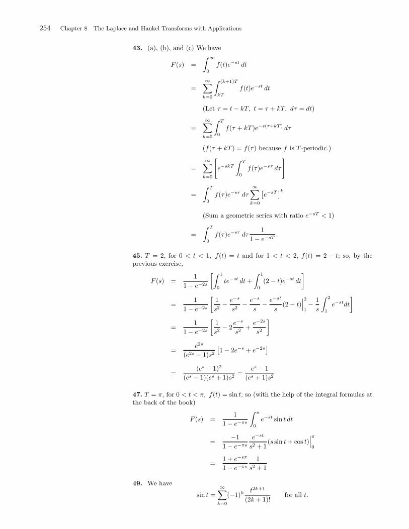
254 Chapter 8 The Laplace and Hankel Transforms with Applications
43. (a), (b), and (c) We have
F (s) =
∫ ∞
0
f(t)e−st dt
=∞∑
k=0
∫ (k+1)T
kT
f(t)e−st dt
(Let τ = t− kT, t = τ + kT, dτ = dt)
=
∞∑
k=0
∫ T
0
f(τ + kT )e−s(τ+kT ) dτ
(f(τ + kT ) = f(τ ) because f is T -periodic.)
=
∞∑
k=0
[e−skT
∫ T
0
f(τ )e−sτ dτ
]
=
∫ T
0
f(τ )e−sτ dτ
∞∑
k=0
[e−sT
]k
(Sum a geometric series with ratio e−sT < 1)
=
∫ T
0
f(τ )e−sτ dτ1
1 − e−sT.
45. T = 2, for 0 < t < 1, f(t) = t and for 1 < t < 2, f(t) = 2 − t; so, by theprevious exercise,
F (s) =1
1 − e−2s
[∫ 1
0
te−st dt+
∫ 1
0
(2 − t)e−st dt
]
=1
1 − e−2s
[1
s2− e−s
s2− e−s
s− e−st
s(2 − t)
∣∣∣2
1− 1
s
∫ 2
1
e−stdt
]
=1
1 − e−2s
[1
s2− 2
e−s
s2+e−2s
s2
]
=e2s
(e2s − 1)s2[1 − 2e−s + e−2s
]
=(es − 1)2
(es − 1)(es + 1)s2=
es − 1
(es + 1)s2
47. T = π, for 0 < t < π, f(t) = sin t; so (with the help of the integral formulas atthe back of the book)
F (s) =1
1 − e−πs
∫ π
0
e−st sin t dt
=−1
1 − e−πs
e−st
s2 + 1(s sin t+ cos t)
∣∣∣π
0
=1 + e−sπ
1 − e−πs
1
s2 + 1
49. We have
sin t =
∞∑
k=0
(−1)k t2k+1
(2k + 1)!for all t.
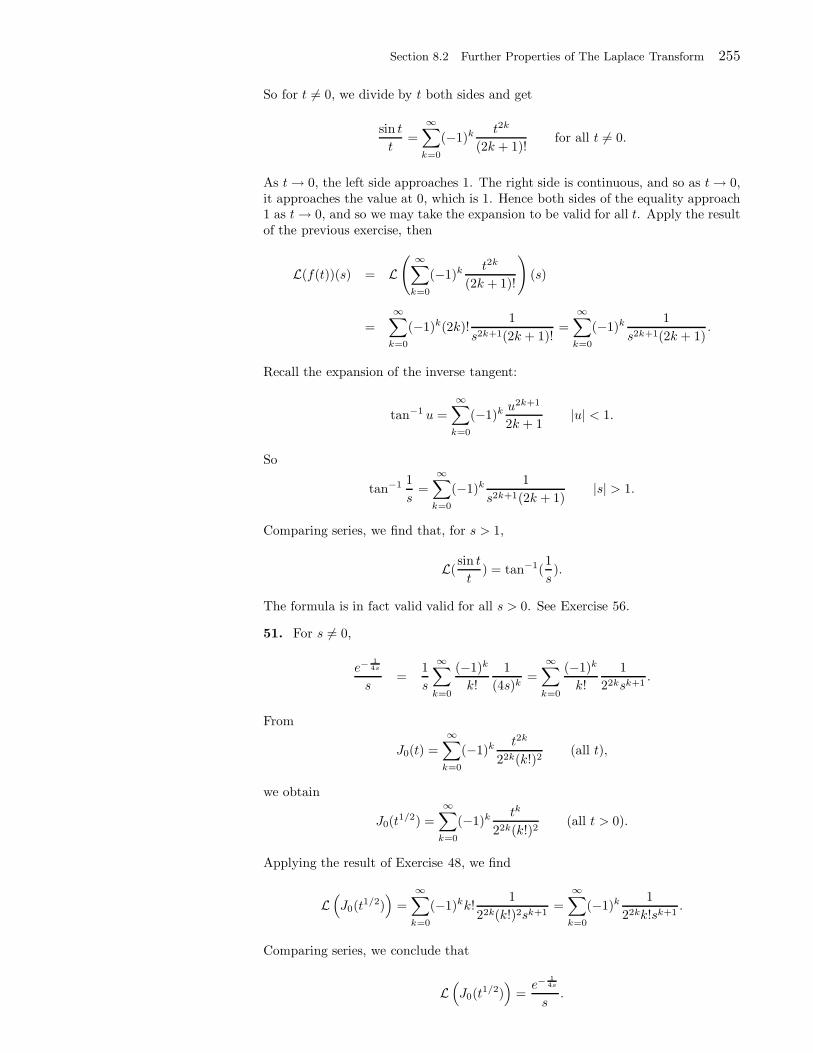
Section 8.2 Further Properties of The Laplace Transform 255
So for t 6= 0, we divide by t both sides and get
sin t
t=
∞∑
k=0
(−1)k t2k
(2k + 1)!for all t 6= 0.
As t→ 0, the left side approaches 1. The right side is continuous, and so as t→ 0,it approaches the value at 0, which is 1. Hence both sides of the equality approach1 as t→ 0, and so we may take the expansion to be valid for all t. Apply the resultof the previous exercise, then
L(f(t))(s) = L( ∞∑
k=0
(−1)k t2k
(2k + 1)!
)(s)
=
∞∑
k=0
(−1)k(2k)!1
s2k+1(2k + 1)!=
∞∑
k=0
(−1)k 1
s2k+1(2k + 1).
Recall the expansion of the inverse tangent:
tan−1 u =
∞∑
k=0
(−1)k u2k+1
2k + 1|u| < 1.
So
tan−1 1
s=
∞∑
k=0
(−1)k 1
s2k+1(2k + 1)|s| > 1.
Comparing series, we find that, for s > 1,
L(sin t
t) = tan−1(
1
s).
The formula is in fact valid valid for all s > 0. See Exercise 56.
51. For s 6= 0,
e−14s
s=
1
s
∞∑
k=0
(−1)k
k!
1
(4s)k=
∞∑
k=0
(−1)k
k!
1
22ksk+1.
From
J0(t) =
∞∑
k=0
(−1)k t2k
22k(k!)2(all t),
we obtain
J0(t1/2) =
∞∑
k=0
(−1)k tk
22k(k!)2(all t > 0).
Applying the result of Exercise 48, we find
L(J0(t
1/2))
=
∞∑
k=0
(−1)kk!1
22k(k!)2sk+1=
∞∑
k=0
(−1)k 1
22kk!sk+1.
Comparing series, we conclude that
L(J0(t
1/2))
=e−
14s
s.
256 Chapter 8 The Laplace and Hankel Transforms with Applications
53. We have
L(
1
a√πe−
t2
4a2
)(s) =
1
a√π
∫ ∞
0
e−ste−t2
4a2 dt
=1
a√π
∫ ∞
0
e−( t2a +as)2
+a2s2
dt
=1
a√πea2s2
∫ ∞
0
e−( t2a +as)2
dt
(Let T =t
2a+ as, dT =
1
2adt.)
=1√πea2s2
∫ ∞
as
e−T 2
2 dT
= ea2s2 2√π
∫ ∞
as
e−t2 dt
= ea2s2
erfc (as) .
54. Note that, for a > 0,
L (f(at)) (s) =
∫ ∞
0
e−stf(at) dt
=1
a
∫ ∞
0
e−sa tf(t) dt =
1
aL (f(t))
( sa
).
Using this and Exercise 52, we find
L (erf(at)) (s) =1
a
1sa
es2
4a2 erfc( s
2a
)=
1
se
s2
4a2 erfc( s
2a
).
55. Let F (s) denote the Laplace tarnsform of f . Then
∫ ∞
s
F (u) du =
∫ ∞
s
∫ ∞
0
f(t)e−ut dt du
=
∫ ∞
0
∫ ∞
s
e−utf(t) du dt
=
∫ ∞
0
(−1
t
)e−ut
∣∣∣∞
sf(t) du dt
=
∫ ∞
0
1
te−stf(t) du dt
= L(f(t)
t
)(s).
57. Bessel’s equation of order 0 is
xy′′ + y′ + xy = 0.
Section 8.2 Further Properties of The Laplace Transform 257
Applying the Laplace transform, we obtain
L(xy′′) + L(y′) + L(xy) = 0;
− d
dsL(y′′) + L(y′) − d
dsL(y) = 0
− d
ds
[s2Y − sy(0) − y′(0)
]+ sY − y(0) − Y ′ = 0
[− 2sY − s2Y ′ + sy(0)
]+ sY − y(0) − Y ′ = 0
−Y ′(1 + s2) − sY = 0
Y ′ +s
1 + s2Y = 0.
An integating factor for this first order linear differential equation is
eR
s
1+s2 ds= e
12 ln(1+s2) =
√1 + s2
After multiplyig by the integrating factor, the equation becmes
d
ds[√
1 + s2Y ] = 0 .
Integrating both sides, we get
√1 + s2Y = K
or
Y =K√
1 + s2,
where K is a constant.From Exercise 50, y = KJ0(t).
258 Chapter 8 The Laplace and Hankel Transforms with Applications
Solutions to Exercises 8.3
1. The solution is the same as Example 2. Simply take T0 = 70 in that example.
3. The problem is the same as in Example 2, except that the boundary value atx = 0 is delayed by 2 time units. Hence the solution is the same as in Example 2,delayed by 2 time units:
u(x, t) =
0 if 0 < t < 2
U(x, t− 2) if t > 2,
where U(x, t) is the solution in Example 2. Thus
u(x, t) =
0 if 0 < t < 2
100 erfc(
x2√
t−2
)if t > 2,
5. Using the formula from Example 3, we get
u(x, t) =
∫ t
0
(t − τ )[τ − (t − x)U0(τ − x)] dτ
=
∫ t
0
(t − τ )τ dτ −∫ t
0
(t − τ )(τ − x)(U0(τ − x) dτ
=t
2τ2 − 1
3τ3∣∣∣t
0−∫ t
0
(t− τ )(τ − x)U0(τ − x) dτ
=t3
3!−∫ t
0
(t− τ )(τ − x)U0(τ − x) dτ
Note that U 0(τ −x) = 1 if τ > x and 0 if τ < x. So the integral is 0 if t < x (sincein this case τ ≤ t < x). If x < τ < t, then
∫ t
0
(t − τ )(τ − x)U0(τ − x) dτ
=
∫ t
x
(t− τ )(τ − x) dτ
=
∫ t
x
(tτ − tx− τ2 + τx) dτ
=1
2tτ2 − txτ − 1
3τ3 +
1
2τ2x
∣∣∣t
x
=1
2t3 − t2x− 1
3t3 +
1
2t2x− 1
2tx2 + tx2 +
1
3x3 − 1
2x3
=1
6t3 − 1
2t2x+
1
2tx2 − 1
6x3
=1
6(t − x)3
Hence
u(x, t) =
16 t
3 if t < x
16t3 − 1
6(t− x)3 if t > x,
Section 8.3 The Laplace Transform Method 259
or
u(x, t) =1
6t3 − 1
6(t − x)3 U 0(t − x).
7. Let u1 be the solution of
∂2u
∂t2=∂2u
∂x2, x > 0, t > 0,
u(0, t) = 0, t > 0,
u(x, 0) = 0, ∂u∂t
(x, 0) = 1, x > 0 .
Let u2 be the solution of
∂2u
∂t2=∂2u
∂x2− g, x > 0, t > 0,
u(0, t) = 0, t > 0,
u(x, 0) = 0, ∂u∂t (x, 0) = 0, x > 0 .
You can check that u = u1 + u2 is the desired solution of
∂2u
∂t2=∂2u
∂x2− g, x > 0, t > 0,
u(0, t) = 0, t > 0,
u(x, 0) = 0, ∂u∂t (x, 0) = 1, x > 0 .
Now u2 is solved in Example 4. We can write
u2(x, t) = −g2(t2 − (t− x)2 U0(t− x)).
To find u1, we go back to (9),use the initial conditions u(x, 0) = 0 and ∂u∂t (x, 0) = 1.
Then the equation becomes
s2U(x, s) − su(x, 0) − ut(x, 0) = Uxx(x, s)
s2U(x, s) − 1 = Uxx(x, s);
Uxx(x, s) − s2U(x, s) = −1;
The associated homogeneous equation has general solution
A(s)e−sx +B(s)esx
Since the transform has to be bounded as s → ∞, we take B(s) = 0 and thesolution becomes A(s)e−sx. It is easy to verify that a particular solution of
Uxx(x, s) − s2U(x, s) = −1
is 1/s2 (constant functionin x). Hence
U(x, s) = A(s)e−sx +1
s2.
Using the initial conditions,
U(0, s) = 0 ⇒ A(s) = − 1
s2;
U(x, s) =−e−sx + 1
s2.
260 Chapter 8 The Laplace and Hankel Transforms with Applications
Taking inverse Laplace transforms,
u1(x, t) = L−1(−e−sx
s2
)+ L−1
( 1
s2
);
= −(t − x)U0(t − x) + t.
u(x, t) = −(t − x)U0(t − x) + t− g
2(t2 − (t− x)2 U0(t− x))
9. Transforming the problem, we find (see Exercise 7 for similar details)
s2U(x, s) − su(x, 0) − ut(x, 0) = Uxx(x, 0);
s2U(x, s) − 1 = Uxx(x, 0);
Uxx(x, 0) − s2U(x, s) = −1;
U(x, s) = A(s)e−sx +1
s2;
U(0, s) = L(sin t) =1
1 + s2;
⇒ A(s) +1
s2=
1
1 + s2
⇒ A(s) =1
1 + s2− 1
s2
U(x, s) =
[1
1 + s2− 1
s2
]e−sx +
1
s2
u(x, t) = t− (t− x)U0(t− x) + sin(t − x)U0(t− x).
11. Use (8) with f(τ ) = δ0(τ ). Then
u(x, t) =x
2c√π
e−x2
4c2t
t3/2.
13. Verify that
u(x, t) = u1(x, t) + u2(x, t),
where u1 is a solution of
ut = uxx;
u(0, t) = 70;
u(x, 0) = 70;
and u2 is a solution of
ut = uxx;
u(0, t) = 30;
u(x, 0) = 0.
Section 8.3 The Laplace Transform Method 261
It is immediate that the solution of the first problem is u1 = 70. The solution ofthe second problem is similar to Example 2:
u2(x, t) = 30 erfc
(x
2√t
).
15. You can verify that the solution of the problem
∂u
∂t= c2
∂2u
∂x2, x > 0, t > 0,
u(0, t) = T0, t > 0,
u(x, 0) = T1, x > 0,
is given by u1 + u2, where u1 is a solution of
∂u
∂t= c2
∂2u
∂x2, x > 0, t > 0,
u(0, t) = T1, t > 0,
u(x, 0) = T1, x > 0,
and u2 is a solution of
∂u
∂t= c2
∂2u
∂x2, x > 0, t > 0,
u(0, t) = T0 − T1, t > 0,
u(x, 0) = 0, x > 0.
We have u1 = T1 and, by Example 2,
u2 = (T0 − T1) erfc
(x
2c√t
).
262 Chapter 8 The Laplace and Hankel Transforms with Applications
Solutions to Exercises 8.4
1. (a) Let z2 = x, u(z, t) = u(z2, t) = u(x, t). Then
2zdz
dx= 1 or
dz
dx=
1
2z.
So
∂
∂xu(x, t) =
∂
∂xu(z, t) =
∂u
∂z
dz
dx=∂u
∂z
1
2z
Similarly,
∂2u
∂x2=
∂2
∂x
[∂u
∂z
1
2z
]
=d
dx
(1
2z
)∂u
∂z+
1
2z
∂
∂x
(∂u
∂z
)
=−1
2z2
dz
dx
∂u
∂z+
1
2z
∂2u
∂z2
dz
dx
=−1
4z3
∂u
∂z+
1
4z2
∂2u
∂z2
(b) Substituting what we found in (a) into (6) and using u in place of u to simplifynotation, we get
utt = g
[z2
[− 1
4z3uz +
1
4z2uzz
]+
1
2zuz
]
=g
4
[uzz +
1
zuz
]
3. Use the identity 2νu Jν(u) = Jν−1(u) + Jν+1(u). Then
Hν(1
xf(x))(s) = s
∫ ∞
0
f(x)1
sxJν(sx)x dx
=s
2ν
∫ ∞
0
f(x)2ν
sxJν(sx)x dx
=s
2ν
∫ ∞
0
f(x)[Jν−1(sx) + Jν+1(sx)]x dx
=s
2ν[Hν−1(f)(s) + Hν+1(f)(s)]
Section 8.4 The Hankel Transform with Applications 263
5. Using Exercise 9 of Section 4.3, we find
H0(x2N U0(a− x))(s) =
∫ ∞
0
x2N U0(a− x)J0(sx)x dx
=
∫ a
0
J0(sx)x2N+1 dx
(change variables sx ↔ x)
=1
s2N+2
∫ as
0
x2N+1J0(x) dx
=1
s2N+2
N∑
n=0
(−1)n2N N !
(N − n)!x2N+1−nJn+1(x)
∣∣∣as
0
=1
s2N+2
N∑
n=0
(−1)n2N N !
(N − n)!(as)2N+1−nJn+1(as)
=
N∑
n=0
(−1)n2N N !
(N − n)!
a2N+1−n
s1+nJn+1(as)
7. Letting a → 0 in (b) of Exercise 6, the right side tends to 1/s while the left sidetends to H0(
1x)(s). (This is not a proof! but it does yield the correct transform of
1/x.) If we apply the transform directly and change variables, we obtain
H0(1
x)(s) =
∫ ∞
0
1
xJ0(sx)x dx =
∫ ∞
0
J0(sx) dx =1
s
∫ ∞
0
J0(x) dx.
It is a fact (see the proof below) that
I =
∫ ∞
0
J0(x) dx = 1
Using this fact, we obtain the desired formula for H0(1x)(s).
Let us outline a proof of the evaluation of the integral I. Refer to Section 4.9for the properties of Bessel functions.(a) Using the aymptotic formula for J0 and the alternating series test, show thatthe integral of J0(x) is (conditionally) convergent. (It is the alternating sum ofareas of arches that are tending to 0.)(b) Because the integral is converging, we can write
I = limn→∞
∫ n
0
J0(x) dx = limn→∞
In.
Now use the integral representation of J0 to conclude that
In =1
π
∫ n
0
∫ π
0
cos(x sin t) dt dx.
Write the inner integral as
∫ π
0
cos(x sin t) dt =
∫ π/2
0
cos(x sin t) dt+
∫ π
π/2
cos(x sin t) dt.
In the second integral on the right, make the change of variables t ↔ π − t andconclude that ∫ π
0
cos(x sin t) dt = 2
∫ π/2
0
cos(x sin t) dt
264 Chapter 8 The Laplace and Hankel Transforms with Applications
and so, after interchanging the order of integration,
In =2
π
∫ π/2
0
∫ n
0
cos(x sin t) dx dt
=2
π
∫ π/2
0
sin(x sin t)
sin t
∣∣∣n
0dt =
2
π
∫ π/2
0
sin(n sin t)
sin tdt
Make the change of variables sin t↔ u, cos t dt = du ⇒ dt = 1√1−u2du. So
In =2
π
∫ 1
0
sin(nu)
u
1√1 − u2
du.
This integral is quite difficult to evaluate, but there is a closely related integral thatwe can evaluate in the limit; namely,
Sn =2
π
∫ 1
0
sin(nu)
udu =
2
π
∫ n
0
sinu
udu,
after making the change of variables nu ↔ u. Hence, using the famous integral∫∞0
sin uu
du = π2, we obtain
limn→∞
Sn =2
π
∫ n
0
sinu
udu =
2
π
∫ ∞
0
sinu
udu = 1.
To complete the proof, we will show that
limn→∞
In − Sn = 0;
from this it will follow that
limn→∞
In = limn→∞
Sn = 1,
as desired. For this, we will need the Riemann-Lebesgue lemma from Section 2.8.We have
In−Sn =2
π
∫ 1
0
[sin(nu)
u
1√1 − u2
− sin(nu)
u
]du =
2
π
∫ 1
0
sin(nu)1
u
[1√
1 − u2− 1
]du.
Let
f(x) =
1x
[1√
1−x2 − 1]
if 0 < x < 1
0 if 1 < x < 2π.
We claim that f(x) integrale on [0, 2π]. Once the claim is established, it will followfrom the Riemann-Lebesgue lemma that
limn→∞
∫ 2π
0
f(u) sinnu du = 0,
which is what we want to show. The function f seems to have two problems in0, 2π]; one at x = 0 and one at x = 1. At x = 1, the problem comes from1/sqrt1 − x, which is an integrable function. At x = 0, we have
limx→0
f(x) = limx→0
1
x
[1√
1 − x2− 1
]
= limx→0
1
x
[1 −
√1 − x2
√1 − x2
]
= limx→0
1
x
[(1 −
√1 − x2)(1 +
√1 − x2)√
1 − x2(1 +√
1 − x2)
]
= limx→0
x√1 − x2(1 +
√1 − x2)
= 0.
Section 8.4 The Hankel Transform with Applications 265
So at x = 0, the function f(x) is nice and bounded. In conclusion, f is integrbaleon [0, 2π]. In fact, if you plot the graph of f on (0, 1), you will notice that it ispositive and tends to 0 at 0. It is not hard to show that
∫ 1
0
1
x
(1√
1 − x2− 1
)dx = − ln
(1 +
√1 − x2
) ∣∣∣1
0= ln2.
We can now use the improper integral
∫ ∞
0
J0(x) dx = 1
and the recurrence relation (5), Section 4.8, to derive
∫ ∞
0
Jn(x) dx = 1
for all n ≥ 0. Indeed, for n = 1, the formula follows from
∫ ∞
0
J1(x) dx = −J0(x)∣∣∣∞
0= 1.
For n ≥ 2, use (5), Section 4.8. We also have the interesting identity: for n ≥ 1,
∫ ∞
0
Jn(x)
xdx =
1
n,
which follows from (6), Section 4.8.The techniques that we used can be applied with ease to obtain the Fourier
transform of J0(x) and thus provide a different way to compute the integral
∫ ∞
0
J0(x) dx = 1
Indeed, back to the integral reprepsentation
J0(x) =1
π
∫ π
0
cos(x sin t) dt.
Making the change of variables t− π2 and then the change of variable u = sin t, we
obtain
J0(x) =1
π
∫ π2
−π2
cos(x sin t) dt
=1
π
∫ 1
−1
1√1 − u2
cos(xu) du.
Let
f(u) =
√2π
1√1−u2 if |u| < 1,
0 if |u| > 1.
Then the integral representation of J0(x) shows that
J0(x) = F(f)(x),
where F(f) is teh Fourier transform of f . Thus, F−1(J0) = F−1(F(f)) = f . ButJ0 is even, so F−1(J0) = F(J0). Thus the formula
F(J0)(w) =
√2π
1√1−w2
if |w| < 1,
0 if |w| > 1.
266 Chapter 8 The Laplace and Hankel Transforms with Applications
Using this formula at w = 0, we get
1√2π
∫ ∞
−∞J0(x) dx =
√2
π⇒
∫ ∞
−∞J0(x) dx = 2.
8. (a), (b), (c) We have
J0(x) =
∞∑
k=0
(−1)k
(k!)2
(x2
)2k
;
H0(e−a2x2
) =
∫ ∞
0
e−a2x2∞∑
k=0
(−1)k
(k!)2
(sx2
)2k
x dx
=
∞∑
k=0
(−1)k
(k!)2s2k
22k
∫ ∞
0
e−a2x2
x2kx dx
(Substitute x2 =t
a2, a2x2 = t, 2a2x dx = dt, x dx =
dt
2a2)
=1
a2
∞∑
k=0
(−1)k
(k!)2s2k
22k+1
∫ ∞
0
e−t
(t1/2
a
)2k
dt
=1
a2
∞∑
k=0
(−1)k
(k!)2s2k
22k+1a2k
∫ ∞
0
e−ttk dt
=1
2a2
∞∑
k=0
(−1)k
(k!)2s2k
(4a2)k
=k!︷ ︸︸ ︷∫ ∞
0
e−ttk dt
=1
2a2
∞∑
k=0
(−1)k
k!
s2k
(4a2)k=e−
s2
4a2
2a2
9. (a) The chain starts to move from rest with an initial velocity of v(x) =√x.
(b) We have A ≡ 0 and
B(s) =2√gs
H0(1/z)(s) =2√gs2
.
So
u(x, t) =2√g
∫ ∞
0
sin
(√g
2st
)J0
(√xs) 1
sds.
13. Similar to Example 1.
12. We have to solve
Utt = −c2s2U
Section 8.4 The Hankel Transform with Applications 267
The solution is
U(s, t) = A(s) cos(cst) +B(s) sin(cst);
U(s, 0) = F (s) ⇒ A(s) = F (s);
Ut(s, 0) = G(s) ⇒ csB(s) = G(s)
⇒ B(s) =G(s)
cs;
U(s, t) = F (s) cos(cst) +G(s)
cssin(cst).
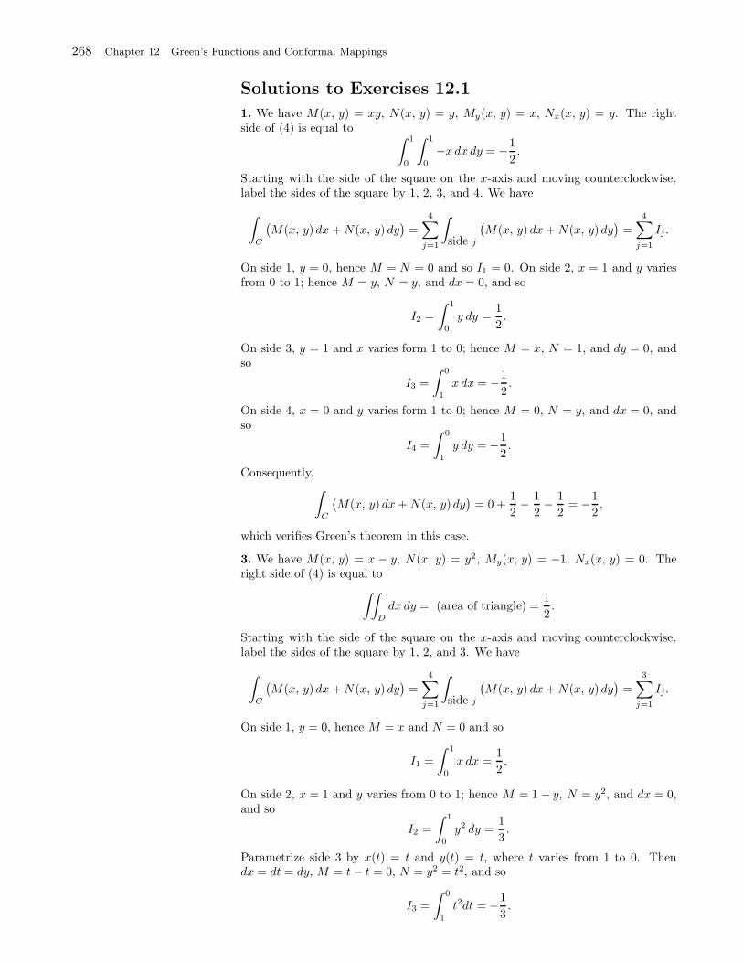
268 Chapter 12 Green’s Functions and Conformal Mappings
Solutions to Exercises 12.1
1. We have M(x, y) = xy, N(x, y) = y, My(x, y) = x, Nx(x, y) = y. The rightside of (4) is equal to ∫ 1
0
∫ 1
0
−x dx dy = −1
2.
Starting with the side of the square on the x-axis and moving counterclockwise,label the sides of the square by 1, 2, 3, and 4. We have
∫
C
(M(x, y) dx +N(x, y) dy
)=
4∑
j=1
∫
side j
(M(x, y) dx+N(x, y) dy
)=
4∑
j=1
Ij.
On side 1, y = 0, hence M = N = 0 and so I1 = 0. On side 2, x = 1 and y variesfrom 0 to 1; hence M = y, N = y, and dx = 0, and so
I2 =
∫ 1
0
y dy =1
2.
On side 3, y = 1 and x varies form 1 to 0; hence M = x, N = 1, and dy = 0, andso
I3 =
∫ 0
1
x dx = −1
2.
On side 4, x = 0 and y varies form 1 to 0; hence M = 0, N = y, and dx = 0, andso
I4 =
∫ 0
1
y dy = −1
2.
Consequently,∫
C
(M(x, y) dx+N(x, y) dy
)= 0 +
1
2− 1
2− 1
2= −1
2,
which verifies Green’s theorem in this case.
3. We have M(x, y) = x − y, N(x, y) = y2 , My(x, y) = −1, Nx(x, y) = 0. Theright side of (4) is equal to
∫∫
D
dx dy = (area of triangle) =1
2.
Starting with the side of the square on the x-axis and moving counterclockwise,label the sides of the square by 1, 2, and 3. We have
∫
C
(M(x, y) dx +N(x, y) dy
)=
4∑
j=1
∫
side j
(M(x, y) dx+N(x, y) dy
)=
3∑
j=1
Ij.
On side 1, y = 0, hence M = x and N = 0 and so
I1 =
∫ 1
0
x dx =1
2.
On side 2, x = 1 and y varies from 0 to 1; hence M = 1 − y, N = y2, and dx = 0,and so
I2 =
∫ 1
0
y2 dy =1
3.
Parametrize side 3 by x(t) = t and y(t) = t, where t varies from 1 to 0. Thendx = dt = dy, M = t− t = 0, N = y2 = t2, and so
I3 =
∫ 0
1
t2dt = −1
3.
Section 12.1 Green’s Theorem and Identities 269
Consequently,∫
C
(M(x, y) dx+N(x, y) dy
)=
1
2+
1
3− 1
3=
1
2,
which verifies Green’s theorem in this case.
5. We have M(x, y) = 0, N(x, y) = x, My(x, y) = 0, Nx(x, y) = 1. The right sideof (6) is equal to
∫∫
D
dx dy = (area of annular region) = π − π
4=
3π
4.
We have∫
Γ
(M(x, y) dx+N(x, y) dy
)=
∫
C2
+
∫
C1
(M(x, y) dx +N(x, y) dy
)= I1 + I2.
Parametrize C1 by x = cos t, y = sin t, 0 ≤ t ≤ 2π, dx = − sin t dt, dy = cos t.Hence
I1 =
∫ 2π
0
cos2 t dt = π.
Parametrize C2 by x = 12 cos t, y = 1
2 sin t, t varies from 2π to 0, dx = −12 sin t dt,
dy = 12 cos t. Hence
I2 =1
4
∫ 0
2π
dt == −∫ 2π
0
1
4cos2 t dt = −π
4.
Consequently, ∫
Γ
(M(x, y) dx+N(x, y) dy
)= π − π
4=
3π
4,
which verifies Green’s theorem in this case.
7. We have M(x, y) = −yx2+y2 , N(x, y) = x
x2+y2 ,
My(x, y) =−x2 − y2 + 2y2
(x2 + y2)2=
−x2 + y2
(x2 + y2)2,
and
Nx(x, y) =−x2 + y2
(x2 + y2)2.
The right side of (6) is equal to
∫∫
D
0 dx dy = 0.
We have∫
Γ
(M(x, y) dx+N(x, y) dy
)=
∫
C2
+
∫
C1
(M(x, y) dx +N(x, y) dy
)= I1 + I2.
Parametrize C1 by x = cos t, y = sin t, 0 ≤ t ≤ 2π, dx = − sin t dt, dy = cos t. OnC1, x
2 + y2 = 1; hence
I1 =
∫ 2π
0
(sin2 t+ cos2 t) dt = 2π.
Parametrize C2 by x = 12
cos t, y = 12
sin t, t varies from 2π to 0, dx = −12
sin t dt,dy = 1
2cos t. On C1, x
2 + y2 = 14; hence
I2 = 4
∫ 0
2π
(14
sin2 t+1
4cos2 t
)dt = −
∫ 2π
0
dt = −2π.
270 Chapter 12 Green’s Functions and Conformal Mappings
Consequently, ∫
Γ
(M(x, y) dx+N(x, y) dy
)= 2π − 2π = 0,
which verifies Green’s theorem in this case.
9. Take u(x, y) = y and v(x, y) = x. Then ∇2v = 0, ∇u = (0, 1), ∇v = (1, 0), so∇u · ∇v = 0 and, by (9),
∫
C
y∂x
∂nds =
∫
C
u∂v
∂nds =
∫
Γ
0 ds = 0.
11. Take u(x, y) = x + y and f(x, y) = ex cos y. Then ∇2v = 0, ∇u = (1, 1),∇v = (ex cos y, −ex sin y), so ∇u · ∇v = ex
(cos y − sin y
)and, by (9),
∫
C
y(x + y)∂f
∂nds =
∫∫
D
ex(cos y − sin y
)dx dy
=
∫ 1
0
∫ 1
0
ex(cos y − siny
)dx dy
= ex∣∣∣1
0
(sin y + cos y)
∣∣∣1
0
= (e− 1)(sin 1 + cos 1 − 1).
13. Same solution as in Example 1. Use Theorem 2 instead of Theorem 1.
14. We have M(x, y) = −yx2+y2 , N(x, y) = x
x2+y2 ,
My(x, y) =−x2 + y2
(x2 + y2)2,
and
Nx(x, y) =−x2 + y2
(x2 + y2)2.
Let Γ consits of C (positive orientation) and −Cr (negative orientation). ApplyingTheorem 2, since Nx −My = 0, we have
∫
Γ
Mdx+Ndy = 0.
Hence ∫
C
Mdx+Ndy +
∫
−Cr
Mdx+Ndy = 0
or ∫
C
Mdx+Ndy =
∫
Cr
Mdx+Ndy
where Cr is positively oriented, centered at the origin, with radius r. Thus, in orderto compute the desired integral, it is enough to compute
∫
Cr
Mdx+Ndy.
On Cr, x = r cos t, y = r sin t, dx = −r sin t, dy = r cos t, and x2 + y2 = r2. So
∫
Cr
Mdx+Ndy =
∫ 2π
0
−r sin t(−r sin t) + r cos t(r cos t)
r2=
∫ 2π
0
dt = 2π.
Section 12.1 Green’s Theorem and Identities 271
15. Since u is harmonic, it follows that ∇2u = 0. Switch the notation in (9) v ↔ u,then use ∇2u = 0 and v = 0 on Γ:
∫∫
Ω
(v∇2u+ ∇v · ∇u)dxdy = Γv∂u
∂nds;
∫∫
Ω
∇v · ∇udxdy = 0.
17. We use the 2nd integral in Example 1. Let us parametrize the ellipse byx(t) = a cos t, y(t) = b sin t, dy = b cos t dt, 0 ≤ t ≤ 2π.
Area =
∫
C
x dy =
∫ 2π
0
a cos t b sin t dt
= a b
∫ 2π
0
cos2 t dt = a b
∫ 2π
0
1 + cos(2t)
2dt
= πab.
19. The problem does not have a solution because f(θ) does not satisfy the com-patibility condition (Example 5)
∫ 2π
0
f(θ) dθ = 0.
Indeed ∫ 2π
0
f(θ) dθ =
∫ π
0
sin θ dθ = 2 6= 0.
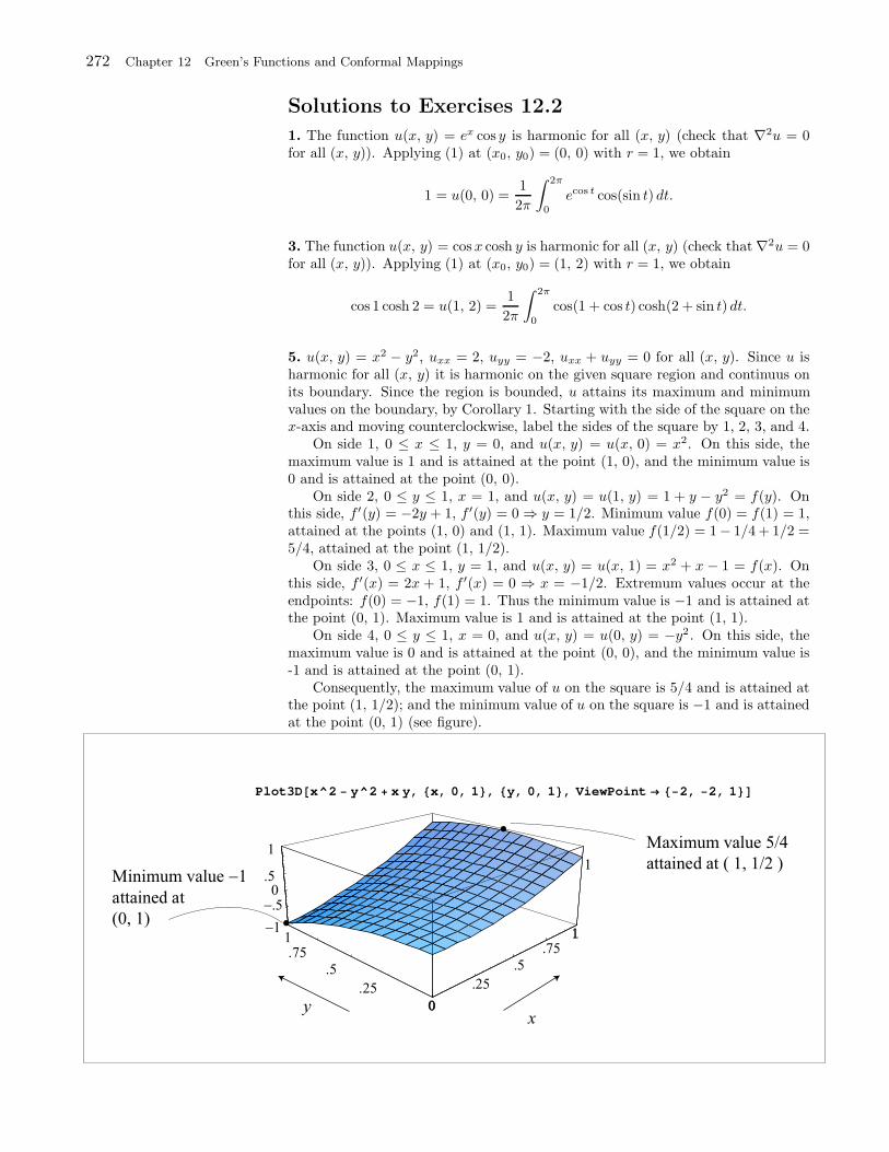
272 Chapter 12 Green’s Functions and Conformal Mappings
Solutions to Exercises 12.2
1. The function u(x, y) = ex cos y is harmonic for all (x, y) (check that ∇2u = 0for all (x, y)). Applying (1) at (x0, y0) = (0, 0) with r = 1, we obtain
1 = u(0, 0) =1
2π
∫ 2π
0
ecos t cos(sin t) dt.
3. The function u(x, y) = cosx cosh y is harmonic for all (x, y) (check that ∇2u = 0for all (x, y)). Applying (1) at (x0, y0) = (1, 2) with r = 1, we obtain
cos 1 cosh 2 = u(1, 2) =1
2π
∫ 2π
0
cos(1 + cos t) cosh(2 + sin t) dt.
5. u(x, y) = x2 − y2, uxx = 2, uyy = −2, uxx + uyy = 0 for all (x, y). Since u isharmonic for all (x, y) it is harmonic on the given square region and continuus onits boundary. Since the region is bounded, u attains its maximum and minimumvalues on the boundary, by Corollary 1. Starting with the side of the square on thex-axis and moving counterclockwise, label the sides of the square by 1, 2, 3, and 4.
On side 1, 0 ≤ x ≤ 1, y = 0, and u(x, y) = u(x, 0) = x2. On this side, themaximum value is 1 and is attained at the point (1, 0), and the minimum value is0 and is attained at the point (0, 0).
On side 2, 0 ≤ y ≤ 1, x = 1, and u(x, y) = u(1, y) = 1 + y − y2 = f(y). Onthis side, f ′(y) = −2y + 1, f ′(y) = 0 ⇒ y = 1/2. Minimum value f(0) = f(1) = 1,attained at the points (1, 0) and (1, 1). Maximum value f(1/2) = 1− 1/4 + 1/2 =5/4, attained at the point (1, 1/2).
On side 3, 0 ≤ x ≤ 1, y = 1, and u(x, y) = u(x, 1) = x2 + x − 1 = f(x). Onthis side, f ′(x) = 2x + 1, f ′(x) = 0 ⇒ x = −1/2. Extremum values occur at theendpoints: f(0) = −1, f(1) = 1. Thus the minimum value is −1 and is attained atthe point (0, 1). Maximum value is 1 and is attained at the point (1, 1).
On side 4, 0 ≤ y ≤ 1, x = 0, and u(x, y) = u(0, y) = −y2 . On this side, themaximum value is 0 and is attained at the point (0, 0), and the minimum value is-1 and is attained at the point (0, 1).
Consequently, the maximum value of u on the square is 5/4 and is attained atthe point (1, 1/2); and the minimum value of u on the square is −1 and is attainedat the point (0, 1) (see figure).
Plot3D x^2 y^2 x y, x, 0, 1 , y, 0, 1 , ViewPoint 2, 2, 1
0
1
0
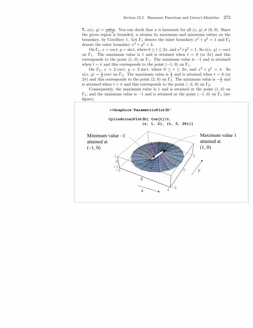
Section 12.2 Harmonic Functions and Green’s Identities 273
7. u(x, y) = xx2+y2 . You can check that u is harmonic for all (x, y) 6= (0, 0). Since
the given region is bounded, u attains its maximum and minimum values on theboundary, by Corollary 1. Let Γ1 denote the inner boundary x2 + y2 = 1 and Γ2
denote the outer boundary x2 + y2 = 4.On Γ1, x = cos t, y = sin t, where 0 ≤ t ≤ 2π, and x2+y2 = 1. So u(x, y) = cos t
on Γ1. The maximum value is 1 and is attained when t = 0 (or 2π) and thiscorresponds to the point (1, 0) on Γ1. The minimum value is −1 and is attainedwhen t = π and this corresponds to the point (−1, 0) on Γ1.
On Γ2, x = 2 cos t, y = 2 sin t, where 0 ≤ t ≤ 2π, and x2 + y2 = 4. Sou(x, y) = 1
2 cos t on Γ2. The maximum value is 12 and is attained when t = 0 (or
2π) and this corresponds to the point (2, 0) on Γ2. The minimum value is −12 and
is attained when t = π and this corresponds to the point (−2, 0) on Γ2.Consequently, the maximum value is 1 and is attained at the point (1, 0) on
Γ1, and the minimum value is −1 and is attained at the point (−1, 0) on Γ1 (seefigure).
<<Graphics‘ParametricPlot3D‘
CylindricalPlot3D[ Cos[t]/r,
r, 1, 2, t, 0, 2Pi]
-2
0
-2
0
2
-1
0
1
0
2
274 Chapter 12 Green’s Functions and Conformal Mappings
Solutions to Exercises 12.3
1. We have ∫
Γ
G(x, y, x0, y0) ds = 0,
because G(x, y, x0, y0) = 0 for all (x, y) on Γ (Theorem 3(ii)).
3. We have ∫
Γ
∂
∂nG(x, y, x0, y0) ds = 2π,
by Theorem 2 with u(x, y) = 1.
5. Let u(x, y) = x, then u is harmonic for all (x, y) and so, by Theorem 2,
∫
Γ
x∂
∂nG(x, y,
1
2,
1
3) ds = 2π
1
2= π.
7. By Theorem 4, with f(x, y) = 1,
∇2
(∫∫
Ω
G(x, y, x0, y0) dx dy
)= 2π.
9. By Theorem 4, with f(x, y) = x2y3,
∇2
(∫∫
Ω
x2y3 G(x, y, x0, y0) dx dy
)= 2πx2
0y30 .
11. Take Γ to be a circle with radius r > 0 and center at (x0, y0). Parametrize Γby x = x0 + r cos t, y = y0 + r sin t, where 0 ≤ t ≤ 2π. We have
(x− x0)2 + (y − y0)
2 = r2 and v(x, y) =1
2ln[(x− x0)
2 + (y − y0)2] = ln r,
and by Proposition 1, Section 12.2,
∂v
∂n=
1
r.
The representation formula of Theorem 1 becomes
u(x0, y0) =1
2π
∫ 2π
0
[u(x0 + r cos t, y0 + r sin t)
1
r− ln r
∂u
∂n
]ds
=1
2π
∫ 2π
0
[u(x0 + r cos t, y0 + r sin t)
1
r
]ds,
because ∫ 2π
0
[∂u∂n
]ds = 0,
by the compatibility condition (Example 5, Section 12.1). Also, ds = r dt and sothe
u(x0, y0) =1
2π
∫ 2π
0
u(x0 + r cos t, y0 + r sin t)dt,
which is Gauss’s mean value property.
Section 12.3 Green’s Functions 275
15. Take Take u = 1 is Theorem 2 and use (2). Then
1 =1
2π
∫
Γ
∂G
∂nds
=1
2π
∫
Γ
∂
∂n
[1
2ln[(x− x0)
2 + (y − y0)2] + h(x, y, x0, y0)
]ds
=1
4π
∫
Γ
∂
∂nln[(x− x0)
2 + (y − y0)2] + h(x, y, x0, y0)ds+
1
2π
∫
Γ
∂
∂nh(x, y, x0, y0)ds
=1
4π
∫
Γ
∂
∂nln((x− x0)
2 + (y − y0)2)ds,
because h is harmonic so the compatibility condition implies that
∫
Γ
∂
∂nh(x, y, x0, y0)ds = 0.
276 Chapter 12 Green’s Functions and Conformal Mappings
Solutions to Exercises 12.4
1. The function u(r, θ) = 1 is harmonic in the unit disk and has boundary valuesf(θ) = 1. Use (10) with f(θ) = 1 and you get, for all 0 ≤ r < 1,
1 =1
2π
∫ 2π
0
1− r2
1 + r2 − 2r cos(θ − φ)dθ.
3. For n = 1, 2, . . ., the function u(r, θ) = rn cos nθ is harmonic in the unit diskand has boundary values (when r = 1) f(θ) = cos nθ. Use (10) with f(θ) = cos nθand you get, for all 0 ≤ r < 1,
rn cos nθ =(R2 − r2)
2π
∫ 2π
0
cosnθ
R2 + r2 − 2rR cos(θ − φ)dθ.
5. For n = 1, 2, . . ., the function u(r, θ) = rn cos nθ is harmonic in the disk ofradius R > 0 and has boundary values (when r = R) f(θ) = Rn cos nθ. Use (10)with f(θ) = Rn cosnθ and you get, for all 0 ≤ r < R,
rn cos nθ =Rn(R2 − r2)
2π
∫ 2π
0
cos nθ
R2 + r2 − 2rR cos(θ − φ)dθ.
7. By Theorem 1, Section 4.6, the function u(r, θ) = J0(αnr) is a solution ofPoisson’s problem
∇2u(r, θ) = −α2nJ0(αnr), u(1, θ) = 0,
on the unit disk. is u(r, θ) = J0(αnr). Since the given integral solves the sameproblem, by Theorem 1 of this section, it follows that the integral is equal J0(αnr).
Section 12.5 Analytic Functions 277
Solutions to Exercises 12.5
1. (a) (3 + 2i)(2 − i) = 6 − 3i+ 4i− 2i2 = 8 + i.(b) (3 − i)(2 − i) = (3 − i)(2 + i) = 7 + i.(c)
1 + i
1 − i=
1 + i
1 − i· 1 − i
1 − i=
(1 + i)(1 + i)
12 + 12= i.
3. (a)1
i=
i
i2=
i
−1= −i.
(b) We have the sequence 1, i, i2 = −1, i3 = −i, i4 = 1, i5 = i, i6 = −1, i7 =−i, i8 = 1, . . .. In general,
in =
1 if n = 4k,
i if n = 4k + 1,
−1 if n = 4k + 2,
−i if n = 4k + 3.
We should note here that (in) is a periodic sequence with period 4. That is, itsvalues repeat every 4 terms.(c) Since i = −i, we obtain
(i)n
= (−1)n(i)n =
1 if n = 4k,
−i if n = 4k + 1,
−1 if n = 4k + 2,
i if n = 4k + 3.
Here too we should note that (in) is a periodic sequence with period 4.
5. (a) Arg (i) = π2 . (b) |i| = 1. (c) i = ei π
2 .
7. (a) Arg (π) = 0. (b) |π| = π. (c) π = π ei·0.
9. (a) Arg (1 + i) = π4. (b) |1 + i| =
√12 + 12 =
√2. (c) 1 + i =
√2 ei·π
4 .
In computing the values of Arg z, just remember that Arg z takesits values in the interval (−π, π]. Consequently, Arg z is not al-ways equal to tan−1(y/x) (see Section 12.5, (8), for the formulathat relates Arg z to tan−1(y/x)). You can use Mathematica toevaluate Arg z and the absolute value of z. This is illustrated bythe following exercises.
278 Chapter 12 Green’s Functions and Conformal Mappings
11. and 13. On Mathematica. You should do these problems by hand and compareyour answers with Mathematica’s answers. Exercise 13 is interesting by hand.
Arg 1 I
3
4
Abs 1 I
2
Sqrt 2 Exp 3 Pi 4 I
234
Simplify %
1
Arg 1 I ^2
2
Abs 1 I ^2
2
15. The complex number z = cosα+ i sinα is unimodular; that is, it has modulusequal to 1. Ths follows from
|z| =√
cos2 α+ sin2 α =√
1 = 1.
So cosα+i sinα is on the unit circle, on the ray at angle α from the positive x-axis.Thus arg z = α. If α is in the interval (−π, π], then we also have Arg z = α, but ifα is not in the interval (−π, π], then by adding or subtracting an integer multipleof 2π we find the unique value of arg z that belongs to (−π, π]. This vaue is Arg z.So Arg z = α+ 2kπ, where k is and integer such that
−π < α+ 2kπ ≤ π.
For example, if α = π2 then Arg z = π
2 . But if α = 5π2 then Arg z = π
2 . Notice thatπ2 = 5π
2 − 2π. Finally, we have
cosα+ i sinα = 1 · eiα = ei(α+2kπ).
17. (a) Apply Euler’s identity, e2i = cos 2 + i sin 2.(b) Use Example 1(d): for z = x+ i y,
sin z = sinx cosh y + i cos x sinhy.
So
sin i = sin 0 cosh 1 + i cos 0 sinh 1 = i sinh 1 = ie− e−1
2.
(c) Use Example 1(e): for z = x+ i y,
cos z = cosx cosh y − i sinx sinhy.
Section 12.5 Analytic Functions 279
So
cos i = cos 0 cosh 1 − i sin 0 sinh1 = cosh 1e+ e−1
2.
(It is real!)(d) Use Example 1(f): for z = x+ i y,
Log z = ln(|z|) + i Arg z.
For z = i, |i| = 1 and Arg i = π2 . So Log i = ln 1 + iπ
2 = iπ2 , because ln 1 = 0.
Remember that there are many branches of the logarithm, log z,and Log z is one of them. All other values of log z differ from Log zby an integer multiple of 2πi. This is because the imaginary partof the logarithm is defined by using a branch of arg z, and thebranches of arg z differ by integer multiples of 2π. (See AppliedComplex Analysis and PDE for more details on the logarithm.) Inparticular, the imaginary part of Log z, which is Arg z, is in theinterval (−π, π].You can use Mathematica to evaluate Log z and ez. This is illus-trated by the following exercises.
19. On Mathematica. You should do these problems by hand and compare youranswers with Mathematica’s answers.
Exp Pi I 2
Exp 2 Pi 2 I
2
Log 1 I
Log 1
ComplexExpand Log 1 I
4
Log 2
2
ComplexExpand Log 1 I ^2
2Log 2
21. We have (−1) · (−1) = 1 but
0 = Log 1 6= Log (−1) + Log (−1) = iπ + iπ = 2iπ.
23. (a) Using the definition of the complex exponential and its properties, we have
|ez | =∣∣ex+i y
∣∣ =∣∣ex · e+i y
∣∣ = |ex| ·∣∣e+i y
∣∣ = ex · 1 = ex,
because |ex| = ex, since ex is always positive (when x is real) and∣∣ei y
∣∣ = 1.More generally, we conclude that
eu = eRe (u)
280 Chapter 12 Green’s Functions and Conformal Mappings
(b) Applying the ”More generally” part, we find that
∣∣eiz∣∣ = eRe (iz) = e−y .
Alternatively,
∣∣eiz∣∣ =
∣∣∣ei(x+i y)∣∣∣ =
∣∣ei x · e−y∣∣ =
∣∣ei x∣∣ ·∣∣e−y
∣∣ = 1 · e−y = e−y.
25. (a) By definition of the cosine, we have
cos(ix) =ei(ix) + e−i(ix)
2=e−x + ex
2= cosh x.
(b) By definition of the since, we have
sin(ix) =ei(ix) − e−i(ix)
2i=e−x − ex
2i= i
ex − e−x
2= i sinhx.
27. (a) Since
sin z = sinx cosh y + i cos x sinhy,
we have the real part u(x, y) = sinx cosh y and the imaginary part v(x, y) =cosx sinh y. To check the Cauchy-Riemann equations, we compute
ux = cosx cosh y, uy = sinx sinh y, vx = − sinx sinhy, vy = cosx cosh y.
It is now clear that ux = vy and that uy = −vx. Hence the Cauchy-Riemannequations hold. Also, all the partial derivatives are continuous functions of (x, y).Hence by Theorem 1, f(z) = sin z is analytic and
f ′(z) = ux + ivx = cos x cosh y − i sinx sinhy = cos z.
(b) We proceed in a similar way. We have
cos z = cosx cosh y − i sinx sinhy.
So u(x, y) = cosx cosh y, v(x, y) = − sinx sinh y, and
ux = − sinx cosh y, uy = cosx sinh y, vx = − cos x sinhy, vy = − sinx cosh y.
We have ux = vy and that uy = −vx. Hence the Cauchy-Riemann equationshold. Also, all the partial derivatives are continuous functions of (x, y). Hence byTheorem 1, f(z) = cos z is analytic and
f ′(z) = ux + ivx = − sinx cosh y − i cos x sinhy = − cos z.
29. (a) Note that, for z = x+ i y 6= 0,
x+ i y
x2 + y2=
z
z · z =1
z.
We claim that this function is not analytic at any z. We have
u =x
x2 + y2, v =
y
x2 + y2;
so
ux =y2 − x2
(x2 + y2)2, uy =
−2xy
(x2 + y2)2, vx =
−2xy
(x2 + y2)2, vy =
x2 − y2
(x2 + y2)2.
Section 12.5 Analytic Functions 281
Since the euqality ux = vy and uy = −vx imply that (x, y) = (0, 0). Hence f isnot analytic at any z = x+ i y.(b) Note that, for z = x+ i y 6= 0,
x− i y
x2 + y2=
z
z · z =1
z,
and ths function is anaytic for all z 6= 0. Using the Cauchy-Riemann equations, wehave
u =x
x2 + y2, v =
−yx2 + y2
;
so
ux =y2 − x2
(x2 + y2)2, uy =
−2xy
(x2 + y2)2, vx =
2xy
(x2 + y2)2, vy =
y2 − x2
(x2 + y2)2.
We have ux = vy and that uy = −vx. Hence the Cauchy-Riemann equations hold.Also, all the partial derivatives are continuous functions of (x, y) 6= (0, 0). Henceby Theorem 1, f(z) = 1
z is analytic for all z 6= 0 and
f ′(z) = ux + ivx =y2 − x2
(x2 + y2)2+ i
2xy
(x2 + y2)2
=(y + ix)2
(x2 + y2)2=
(y + ix)2
(x2 + y2)2
=[i(x− iy)]2
[(x+ i y)(x − i y)]2=
i2
(x+ i y)2=
−1
z2.
31. We leave the verification that u is harmonic as a simple exercise. Before weapply the technique of Example 6, let us look at the function
u(x, y) = x2 − y2 + xy.
The expression x2 − y2 is very familiar: It is the real part of the function
f(z) = z2 = (x+ i y)2 = x2 − y2 + 2i xy.
From this we infer that 2xy is a harmonic conjugate of x2 − y2. Now consider
− i
2f(z) = − i
2z2 = − i
2(x+ i y)2 = xy − i
(x2 − y2)
2.
This function is also entire. Its real part is xy and its imaginary part is y2−x2
2 .
Thus, a harmonic conjugate of xy is y2−x2
2 . Adding the two harmonic conjugates,
we find that a harmonic conjugate of u(x, y) = x2−y2+xy is v(x, y) = 2xy+ y2−x2
2 .So we were able to find a harmonic conjugate taking the imaginary part of an
analytic function that we have guessed and whose real part is the given harmonicfunction u.
Let us now find the harmonic conjugate using the technique of Example 6.Write
u(x, y) = x2 − y2 + xy ux(x, y) = 2x+ y uy(x, y) = −2y + x.
The first equation of the Cauchy-Riemann equations tells us that ux = vy. So
vy(x, y) = 2x+ y.
Integrating with respect to y (treating x as a constant), we find
v(x, y) = 2xy +1
2y2 + c(x),
282 Chapter 12 Green’s Functions and Conformal Mappings
where the constant of integration c(x) is a function of x. The second equation ofthe Cauchy-Riemann equations tells us that uy = −vx. So
vx(x, y) = 2y + c′(x);
−2y − c′(x) = −2y + x;
c′(x) = −x;
c(x) = −1
2x2 + C.
In conclusion,
v(x, y) = 2xy +1
2y2 − 1
2x2 + C,
which matches the previous formula up to a additive constant.
33. We leave the verification that u is harmonic as a simple exercise. The function
u(x, y) = ex cos y
is the real part of the entire function
ez = ex cos y + i ex sin y.
So a harmonic conjugate of ex cos y is ex sin y. (By the same token, a harmonicconjugate of ex sin y is −ex cos y.)
Let us now find the harmonic conjugate using the technique of Example 6.Write
u(x, y) = ex cos y ux(x, y) = ex cos y uy(x, y) = −ex sin y.
The first equation of the Cauchy-Riemann equations tells us that ux = vy. So
vy(x, y) = ex cos y.
Integrating with respect to y (treating x as a constant), we find
v(x, y) = ex sin y + c(x),
where the constant of integration c(x) is a function of x. The second equation ofthe Cauchy-Riemann equations tells us that uy = −vx. So
vx(x, y) = ex sin y + c′(x);
ex sin y + c′(x) = ex sin y;
c′(x) = 0;
c(x) = C.
Hence,
v(x, y) = ex sin y +C,
which matches the previous formula up to a additive constant.
35. The function
f(z) =i
z= i
x− i y
(x + i y)(x − i y)=
y + i x
x2 + y2=
y
x2 + y2+ i
x
x2 + y2
is analytic for all z 6= 0. Its real part
y
x2 + y2
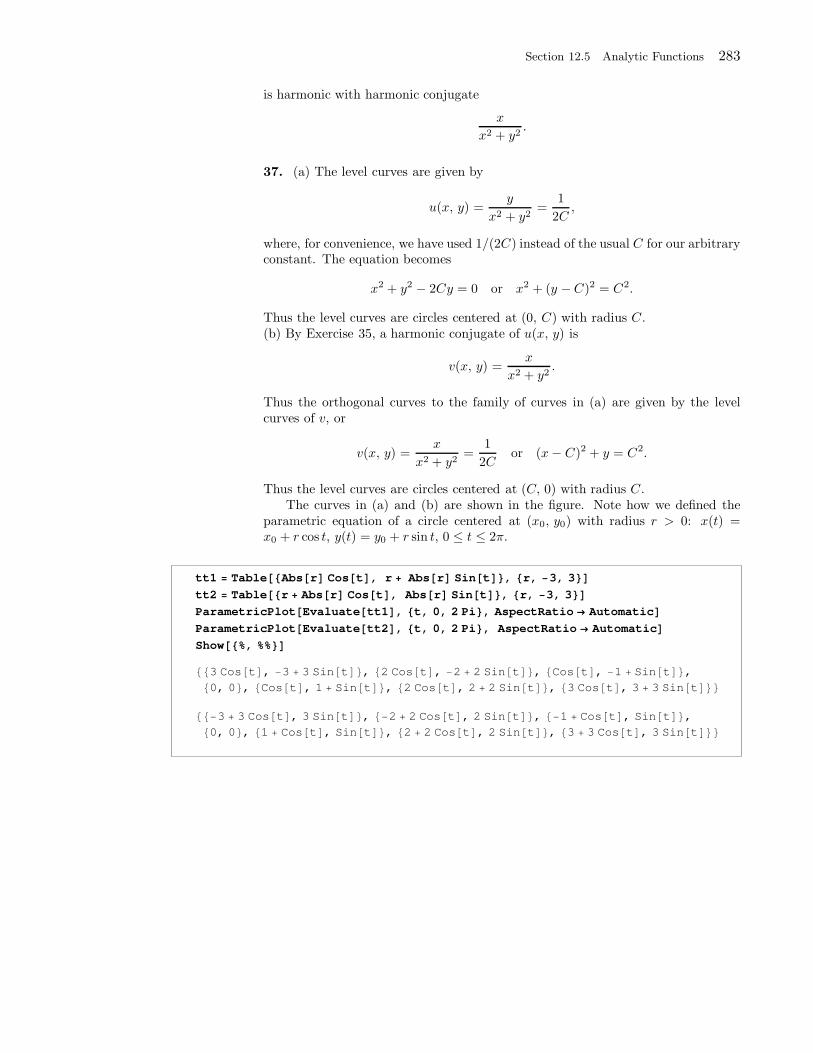
Section 12.5 Analytic Functions 283
is harmonic with harmonic conjugate
x
x2 + y2.
37. (a) The level curves are given by
u(x, y) =y
x2 + y2=
1
2C,
where, for convenience, we have used 1/(2C) instead of the usual C for our arbitraryconstant. The equation becomes
x2 + y2 − 2Cy = 0 or x2 + (y −C)2 = C2.
Thus the level curves are circles centered at (0, C) with radius C.(b) By Exercise 35, a harmonic conjugate of u(x, y) is
v(x, y) =x
x2 + y2.
Thus the orthogonal curves to the family of curves in (a) are given by the levelcurves of v, or
v(x, y) =x
x2 + y2=
1
2Cor (x− C)2 + y = C2.
Thus the level curves are circles centered at (C, 0) with radius C.The curves in (a) and (b) are shown in the figure. Note how we defined the
parametric equation of a circle centered at (x0, y0) with radius r > 0: x(t) =x0 + r cos t, y(t) = y0 + r sin t, 0 ≤ t ≤ 2π.
tt1 Table Abs r Cos t , r Abs r Sin t , r, 3, 3
tt2 Table r Abs r Cos t , Abs r Sin t , r, 3, 3
ParametricPlot Evaluate tt1 , t, 0, 2 Pi , AspectRatio Automatic
ParametricPlot Evaluate tt2 , t, 0, 2 Pi , AspectRatio Automatic
Show %, %%
3 Cos t , 3 3 Sin t , 2 Cos t , 2 2 Sin t , Cos t , 1 Sin t ,
0, 0 , Cos t , 1 Sin t , 2 Cos t , 2 2 Sin t , 3 Cos t , 3 3 Sin t
3 3 Cos t , 3 Sin t , 2 2 Cos t , 2 Sin t , 1 Cos t , Sin t ,
0, 0 , 1 Cos t , Sin t , 2 2 Cos t , 2 Sin t , 3 3 Cos t , 3 Sin t

284 Chapter 12 Green’s Functions and Conformal Mappings
-3 -2 -1 1 2 3
-6
-4
-2
2
4
6
-6 -4 -2 2 4 6
-3
-2
-1
1
2
3
-6 -4 -2 2 4 6
-6
-4
-2
2
4
6
39. (a) and (b) Let n be an integer. The function f(z) = zn is analytic for all zif n ≥ 0, and for z 6= 0 if n < 0. Write z = r eiθ. Then
f(z) = rneinθ = rn (cos nθ + i sinnθ) .
The real and imaginary parts of an analytic function are harmonic; so rn cos nθ andrn sinnθ are harmonic functions. Furthermore, rn sinnθ is a harmonic conjugateof rn cosnθ, and −rn cos nθ is a harmonic conjugate of rn sinnθ.
41. If u(x, y) does not depend on y, then u is a function of x alone. We haveuy = 0 and so uyy = 0. If u is also harmonic, then uxx + uyy = 0. But uyy = 0, souxx = 0. Integrating with respect to x twice, we find u(x, y) = a x+ b.
43. Since u does not depend on y on the boundary, it is reasonable to expect thesame from u inside the region. (This is of course not true if u were not harmonicand constant on each side of the strip. For harmonic functions, we can think ofu as a steady-state solution in a heat problem, as described by Figure 16. Basedon our intuition, we would expect u to be independent of y.) By Exercise 41, wetry u(x, y) = a x + b, where a and b are constants to be determined. Using theboundary conditions,
u(−3, y) = 70 ⇒ −3 a+ b = 70;
u(3, y) = −20 ⇒ 3 a+ b = −20;
⇒ 2b = 50 or b = 25;
⇒ 3a = −45 or a = −15;
⇒ u(x, y) = −15 x+ 25.
At this point, you can check that u is harmonic and satsifies the boundary condi-tions.
45. We reason as in Example 4 and try for a solution a function of the form
u(r, θ) = a Arg z + b,
where z = x+ i y and a and b are constant to be determined. Using the boundary
Section 12.5 Analytic Functions 285
conditions in Figure 18, we find
u(r9 π
10) = 60 ⇒ a
9 π
10+ b = 60;
u(r,3 π
5) = 0 ⇒ a
3 π
5+ b = 0;
⇒ a
(9 π
10− 6 π
10
)= 60 or a =
200
π;
⇒ b = −120;
⇒ u(r, θ) =200
πArg z − 120.
In terms of (x, y), we can use (10) and conclude that, for y > 0,
u(x, y) =200
πcot−1
(x
y
)− 120.
47. We simplify the problem by think of it as the sum of two problems as follows:Let u1 be harmonic in the upper half-plane and equal to T2 on the x-axis, and letu2 be harmonic in the upper half-plane and equal to T1 − T2 on the x-axis on theinterval a < x < b and 0 outside this interval. Let u = u1 +u2. Then u is harmonicin the upper half-plane and equal to T1 on the x-axis on the interval a < x < b andT2 outside this interval (just add the boundary values of u1 and u2). Thus u1 + u2
is the solution to our problem. Now u2 is found in Example 5:
u2(x, y) =T1 − T2
π
[cot−1
(x− b
y
)− cot−1
(x− a
y
)].
To find u1, think of a harmonic function that is equal to T2 on the x-axis. Theanswer is u1(x, y) = T2, and so the solution to our problem is
u(x, y) = T2 +T1 − T2
π
[cot−1
(x− b
y
)− cot−1
(x− a
y
)].
49. As in Exercise 47, we think of the given problem as the sum of two simplersubproblems. Let u1 be harmonic in the upper half-plane and equal to 100 on thex-axis for 0 < x < 1 and 0 for all other values of x. Let u2 be harmonic in theupper half-plane and equal to 20 on the x-axis for −1 < x < 0 and 0 for all othervalues of x. Let u = u1 +u2. Then u is harmonic in the upper half-plane and equalto 20 on the x-axis for −1 < x < 0; 100 for 0 < x < 1; and 0 otherwise. (Just addthe boundary values of u1 and u2.) Thus u1 + u2 is the solution to our problem.Both u1 and u2 are given by Example 5. We have
u1(x, y) =100
π
[cot−1
(x− 1
y
)− cot−1
(x
y
)];
u2(x, y) =20
π
[cot−1
(x
y
)− cot−1
(x+ 1
y
)];
u(x, y) = −80
πcot−1
(x
y
)+
100
πcot−1
(x− 1
y
)− 20
πcot−1
(x+ 1
y
).
286 Chapter 12 Green’s Functions and Conformal Mappings
Solutions to Exercises 12.6
1. (a) f(z) = 1/z is analytic for all z 6= 0, by Theorem 2, Section 12.5, since it isthe quotient of two analytic functions. U(u, v) = uv is harmonic since Uuu = 0,Uvv = 0, so Uuu + Uvv = 0.(b) We have (this was done several times before)
f(z) =x− i y
x2 + y2=
x
x2 + y2− i
y
x2 + y2.
So
Re (f) = u(x, y) =x
x2 + y2and Im(f) = v(x, y) = − y
x2 + y2.
(c) We have
φ(x, y) = U f(z) = U(u(x, y), v(x, y)
)
= U
(x
x2 + y2,
−yx2 + y2
)
=−xy
(x2 + y2)2.
You can verify directly that φ(x, y) is harmonic for all (x, y) 6= (0, 0) or, betteryet, you can apply Theorem 1.
3. (a) f(z) = ez is analytic for all z (Example 2(c), Section 12.5). U(u, v) = u2−v2
is harmonic since Uuu = 2, Uvv = −2, so Uuu + Uvv = 0.(b) We have (Example 2(c), Section 12.5)
f(z) = ex cos y + iex sin y.
So
Re (f) = u(x, y) = ex cos y and Im (f) = v(x, y) = ex sin y.
(c) We have
φ(x, y) = U f(z) = U(u(x, y), v(x, y)
)
= U (ex cos y, ex sin y)
= e2x cos2 y − e2x sin2 y
= e2x cos(2y).
You can verify directly that φ(x, y) is harmonic for all (x, y) or you can note thatφ(x, y) is the real part of the entire function g(z) = e2z.
5. (a) If z is in S, then z = a+ i, y where b ≤ y ≤ c. So
f(z) = ez = ea+i y = eaei y.
The complex number w = eaei y has modulus ea and argument y. As y varies fromb to c, the point w = eaei y traces a circular arc of radius ea, bounded by the tworays at angles b and c.(b) According to (a), the image of z = 1 + i y : 0 ≤ y ≤ π/2 by the mapping ez
is the circular arc with radius e, bounded by the two rays at angles 0 and π/2. Itis thus a quarter of a circle of radius e (see figure).
Similarly, the image of z = 1 + i y : 0 ≤ y ≤ π by the mapping ez is thecircular arc with radius e, bounded by the two rays at angles 0 and π. It is thus asemi-circle of radius e, centered at the origin (see figure).
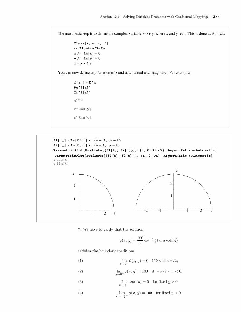
Section 12.6 Solving Dirichlet Problems with Conformal Mappings 287
The most basic step is to define the complex variable z=x+iy, where x and y real. This is done as follows:
Clear x, y, z, f
Algebra‘ReIm‘
x : Im x 0
y : Im y 0
z x I y
You can now define any function of z and take its real and imaginary. For example:
f z_ E^z
Re f z
Im f z
x y
x Cos y
x Sin y
f1 t_ Re f z . x 1, y t
f2 t_ Im f z . x 1, y t
ParametricPlot Evaluate f1 t , f2 t , t, 0, Pi 2 , AspectRatio Automatic
Cos t
Sin t
ParametricPlot Evaluate f1 t , f2 t , t, 0, Pi , AspectRatio Automatic
7. We have to verify that the solution
φ(x, y) =100
πcot−1
(tanx coth y
)
satisfies the boundary conditions
limy→0+
φ(x, y) = 0 if 0 < x < π/2;(1)
limy→0+
φ(x, y) = 100 if − π/2 < x < 0;(2)
limx→π
2−φ(x, y) = 0 for fixed y > 0;(3)
limx→−π
2+φ(x, y) = 100 for fixed y > 0.(4)
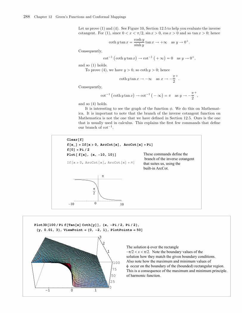
288 Chapter 12 Green’s Functions and Conformal Mappings
Let us prove (1) and (4). See Figure 10, Section 12.5 to help you evaluate the inversecotangent. For (1), since 0 < x < π/2, sinx > 0, cos x > 0 and so tanx > 0; hence
coth y tanx =cosh y
sinh ytanx → +∞ as y → 0+.
Consequently,
cot−1(coth y tanx
)→ cot−1
(+ ∞
)= 0 as y → 0+,
and so (1) holds.To prove (4), we have y > 0, so coth y > 0; hence
coth y tanx→ −∞ as x→ −π2
+.
Consequently,
cot−1(coth y tanx
)→ cot−1
(−∞
)= π as y → −π
2
+,
and so (4) holds.It is interesting to see the graph of the function φ. We do this on Mathemat-
ica. It is important to note that the branch of the inverse cotangent function onMathematica is not the one that we have defined in Section 12.5. Ours is the onethat is usually used in calculus. This explains the first few commands that defineour branch of cot−1.
Clear f
f x_ If x 0, ArcCot x , ArcCot x Pi
f 0 Pi 2
Plot f x , x, 10, 10
If x 0, ArcCot x , ArcCot x
Plot3D 100 Pi f Tan x Coth y , x, Pi 2, Pi 2 ,
y, 0.01, 3 , ViewPoint 0, 2, 1 , PlotPoints 50
-1 0 1
1
2
3
0
25
50
75
100
-1 0 1
1
2
3
Section 12.6 Solving Dirichlet Problems with Conformal Mappings 289
9. We map the region onto the upper half-plane using the mapping f(z) = z2 (seeExample 1). The transformed problem in the uv-plane is ∇2U = 0 with boundaryvalues on the u-axis given by U(u, 0) = 100 if 0 < u < 1 and 0 otherwise. Thesolution in the uv-plane follows from Example 5, Section 12.5. We have
U(u, v) =100
π
[cot−1
(u− 1
v
)− cot−1
(uv
)].
The solution in the xy-plane is φ(x, y) = U f(z). To find the formula in terms of(x, y), we write z = x+ i y, f(z) = z2 = x2 − y2 + 2ixy = (u, v). Thus u = x2 − y2
and v = 2xy and so
φ(x, y) = Uf(z) = U(x2−y2 , 2xy) =100
π
[cot−1
(x2 − y2 − 1
2xy
)− cot−1
(x2 − y2
2xy
)].
11. We map the region onto the upper half-plane using the mapping f(z) = z4.Since f(reiθ) = r4e4iθ, a point z = reiθ on the ray at angle π/4, z = reiπ/4, ismapped to a point on the negative u-axis with modulus r4; that is f(reiπ/4) = −r4.With this observation, we can see that the transformed problem in the uv-plane is∇2U = 0 with boundary values on the u-axis given by U(u, 0) = 50 if −16 < u < 0and 0 otherwise. The solution in the uv-plane follows from Example 5, Section 12.5.We have
U(u, v) =50
π
[cot−1
(uv
)− cot−1
(u+ 64
v
)].
The solution in the xy-plane is φ(x, y) = U f(z). To find the formula in terms of(x, y), we write z = x+ i y,
(u, v) = f(z) = z4 = (x2 − y2 + 2ixy)2 = (x4 + y4 − 6x2y2) + i(4x3y − 4xy3).
Thus u = x4 + y4 − 6x2y2 and v = 4x3y − 4xy3 and so
φ(x, y) = U f(z) = U(x4 + y4 − 6x2y2 , 4x3y − 4xy3)
=50
π
[cot−1
(x4 + y4 − 6x2y2
4x3y − 4xy3
)− cot−1
(x4 + y4 − 6x2y2 + 64
4x3y − 4xy3
)].
13. We map the region onto the upper half-plane using the mapping f(z) = ez
(see Example 2). The points on the x-axis, z = x, are mapped onto the positiveu-axis, since ex > 0 for all x, as follows: f(x) ≥ 1 if x ≥ 0 and 0 < f(x) < 1 ifx < 0. The points on the horizontal line z = x+ iπ are mapped onto the negativeu-axis, since ex+i π = −ex < 0, as follows: f(x + i π) = −ex ≤ −1 if x ≥ 0 and−1 < f(x + i π) = −ex < 0 if x < 0. With these observations, we see that thetransformed problem in the uv-plane is ∇2U = 0 with boundary values on theu-axis given by U(u, 0) = 100 if −1 < u < 1 and 0 otherwise. The solution in theuv-plane follows from Example 5, Section 12.5. We have
U(u, v) =100
π
[cot−1
(u− 1
v
)− cot−1
(u+ 1
v
)].
The solution in the xy-plane is φ(x, y) = U f(z). To find the formula in terms of(x, y), we write z = x+ i y,
(u, v) = f(z) = ez = ex cos y + i ex sin y.
Thus u = ex cos y and v = ex sin y and so
φ(x, y) = U f(z) = U(ex cos y, ex siny)
=100
π
[cot−1
(ex cos y − 1
ex sin y
)− cot−1
(ex cos y + 1
ex sin y
)].
290 Chapter 12 Green’s Functions and Conformal Mappings
15. We map the region onto the upper half-plane using the mapping f(z) = sin z(see Example 3). The transformed problem in the uv-plane is ∇2U = 0 withboundary values on the u-axis given by U(u, 0) = 100 if −1 < u < 1 and 0otherwise. The solution in the uv-plane follows from Example 5, Section 12.5. Wehave
U(u, v) =100
π
[cot−1
(u− 1
v
)− cot−1
(u+ 1
v
)].
The solution in the xy-plane is φ(x, y) = U f(z). To find the formula in terms of(x, y), we write z = x+ i y,
(u, v) = f(z) = sinz = sinx cosh y + i cosx sinh y.
Thus u = sinx cosh y and v = cosx sinh y and so
φ(x, y) = U f(z) = U(sinx cosh y, cos x sinhy)
=100
π
[cot−1
(sinx cosh y − 1
cosx sinh y
)− cot−1
(sinx cosh y + 1
cosx sinh y
)].
17. We map the region onto the upper half-plane using the mapping f(z) = z2 (seeExample 1). The transformed problem in the uv-plane is ∇2U = 0 with boundaryvalues on the u-axis given by U(u, 0) = u if 0 < u < 1 and 0 otherwise. To solve theproblem in the uv-plane, we apply the Poisson integral formula ((5), Section 7.5).We have
U(u, v) =v
π
∫ ∞
−∞
U(s, 0)
(u− s)2 + v2ds =
v
π
∫ 1
0
s
(u− s)2 + v2ds.
Now use your calculus skills to compute this integral. We have
v
π
∫ 1
0
s
(u− s)2 + v2ds =
v
π
∫ 1
0
(s− u)
(s− u)2 + v2ds+
v
π
∫ 1
0
u
(s− u)2 + v2ds
=v
π
[1
2ln[(s− u)2 + v2 ]
∣∣∣1
0+
∫ 1−u
−u
u
t2 + v2dt
](s− u = t)
=v
2πln
(1 − u)2 + v2
u2 + v2+u
πtan−1
(t
v
)∣∣∣1−u
−u
=v
2πln
(1 − u)2 + v2
u2 + v2+u
π
[tan−1
(1 − u
v
)− tan−1
(−uv
)]
=v
2πln
(1 − u)2 + v2
u2 + v2+u
π
[tan−1
(1 − u
v
)+ tan−1
(uv
)].
The solution in the xy-plane is φ(x, y) = U f(z). To find the formula in terms of(x, y), we write z = x+ i y, f(z) = z2 = x2 − y2 + 2ixy = (u, v). Thus u = x2 − y2
and v = 2xy and so
φ(x, y) = U(x2 − y2 , 2xy)
=xy
πln
(1 − (x2 − y2))2 + (2xy)2
(x2 − y2)2 + (2xy)2
+x2 − y2
π
[tan−1
(1 − x2 + y2
2xy
)+ tan−1
(x2 − y2
2xy
)]
=xy
πln
(1 − (x2 − y2))2 + (2xy)2
(x2 + y2)2
+x2 − y2
π
[tan−1
(1 − x2 + y2
2xy
)+ tan−1
(x2 − y2
2xy
)].
Section 12.6 Solving Dirichlet Problems with Conformal Mappings 291
(I verified this solution on Mathematica and it works! It is harmonic and has theright boundary values.)
19. We map the region onto the upper half-plane using the mapping f(z) = ez .The transformed problem in the uv-plane is ∇2U = 0 with boundary values onthe u-axis given by U(u, 0) = u if 0 < u < 1 and 0 otherwise. This was solved inExercise 17. We have
U(u, v) =v
2πln
(1 − u)2 + v2
u2 + v2+u
π
[tan−1
(1 − u
v
)+ tan−1
(uv
)].
To get the solution in the xy-plane, substitute u = ex cos y and v = ex sin y and so
φ(x, y) = U(ex cos y, ex sin y)
=ex sin y
2πln
(1 − ex cos y)2 + (ex sin y)2
(ex cos y)2 + (ex sin y)2
+ex cos y
π
[tan−1
(1 − ex cos y
ex sin y
)+ tan−1
(ex cos y
ex sin y
)]
=ex sin y
2πln
1− 2ex cos y + e2x
e2x+ex cos y
π
[tan−1
(1 − ex cos y
ex sin y
)+ tan−1 (cot y)
]
=ex sin y
2π
[ln(1 − 2ex cos y + e2x) − 2x
]
+ex cos y
π
[tan−1
(1 − ex cos y
ex sin y
)+ tan−1 (cot y)
].
(I verified this solution on Mathematica and it works! It is harmonic and hasthe right boundary values.) The function tan−1 (cot y) is interesting and deservesfurther investigation. In fact, the following figure gives you the answer:
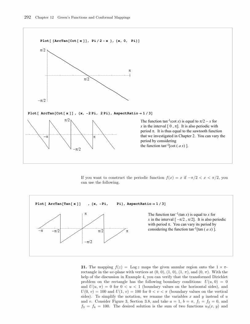
292 Chapter 12 Green’s Functions and Conformal Mappings
Plot ArcTan Cot x , Pi 2 x , x, 0, Pi
Plot ArcTan Cot x , x, 2 Pi, 2 Pi , AspectRatio 1 3
If you want to construct the periodic function f(x) = x if −π/2 < x < π/2, youcan use the following.
Plot ArcTan Tan x , x, Pi, Pi , AspectRatio 1 3
21. The mapping f(z) = Log z maps the given annular region onto the 1 × π-rectangle in the uv-plane with vertices at (0, 0), (1, 0), (1, π), and (0, π). With thehelp of the discussion in Example 4, you can verify that the transformed Dirichletproblem on the rectangle has the following boundary conditions: U(u, 0) = 0and U(u, π) = 0 for 0 < u < 1 (boundary values on the horizontal sides), andU(0, v) = 100 and U(1, v) = 100 for 0 < v < π (boundary values on the verticalsides). To simplify the notation, we rename the variables x and y instead of uand v. Consider Figure 3, Section 3.8, and take a = 1, b = π, f1 = f2 = 0, andf3 = f4 = 100. The desired solution is the sum of two functions u3(x, y) and
Section 12.6 Solving Dirichlet Problems with Conformal Mappings 293
u4(x, y), where
u4(x, y) =
∞∑
n=1
Dn sinhnx sinny;
Dn =2
π sinhn
∫ π
0
100 sinny dy
=−200
nπ sinhn(cosnπ − 1) =
200
nπ sinhn(1 − (−1)n);
u3(x, y) =
∞∑
n=1
Cn sinh[n(1− x)] sinny;
Cn =2
π sinhn
∫ π
0
100 sinny dy
=200
nπ sinhn(1 − (−1)n).
Thus (back to the variables u and v)
U(u, v) = u3 + u4
=
∞∑
n=1
200
nπ sinhn(1 − (−1)n) sinhnu sinnv
+
∞∑
n=1
200
nπ sinhn(1 − (−1)n) sinh[n(1 − u)] sinnv
=200
π
∞∑
n=1
sinnv
n sinhn(1 − (−1)n)
[sinhnu+ sinh[n(1− u)]
]
=400
π
∞∑
n=0
sinh[(2n+ 1)u] + sinh[(2n+ 1)(1 − u)]
(2n+ 1) sinh(2n+ 1)sin[(2n+ 1)v].
To get the solution in the xy-plane, substitute u = 12 ln(x2 +y2) and v = cot−1
(yx
).
The solution takes on a neater form if we use polar coordinates and substitutex2 + y2 = r2 and θ = cot−1
(yx
). Then
φ(x, y) = U(1
2ln(x2 + y2), cot−1
(yx
)) = U(ln r, θ)
=400
π
∞∑
n=0
sinh[(2n+ 1) ln r] + sinh[(2n+ 1)(1 − ln r)]
(2n+ 1) sinh(2n+ 1)sin[(2n+ 1)θ]
= φ(r, θ).
It is interesting to verify the boundary conditions for the solution. For example,when r = 1, we have
φ(1, θ) =400
π
∞∑
n=0
sinh[(2n+ 1)(1)]
(2n+ 1) sinh(2n+ 1)sin[(2n+ 1)θ]
=400
π
∞∑
n=0
sin[(2n+ 1)θ]
(2n+ 1).
This last Fourier sine series is equal to 100 if 0 < θ < π. (see, for example,Exercise 1, Section 2.3). Thus the solution equals to 100 on the inner semi-circular
294 Chapter 12 Green’s Functions and Conformal Mappings
boundary. On the outer circular boundary, r = e, and we have
φ(e, θ) =400
π
∞∑
n=0
sinh(2n+ 1)
(2n+ 1) sinh(2n+ 1)sin[(2n+ 1)θ]
=400
π
∞∑
n=0
sin[(2n+ 1)θ]
(2n+ 1),
which is the same series as we found previously; and thus it equals 100 for 0 < θ < π.Now if θ = 0 or π (which corresponds to the points on the x-axis), then clearlyφ = 0. Hence φ satisfies the boundary conditions, as expected.
23. As in Exercise 21, f(z) = Log z maps the given annular region onto the 1× π-rectangle in the uv-plane with vertices at (0, 0), (1, 0), (1, π), and (0, π). With thehelp of the discussion in Example 4, you can verify that the transformed Dirichletproblem on the rectangle has the following boundary conditions: U(u, 0) = 0and U(u, π) = 0 for 0 < u < 1 (boundary values on the horizontal sides), andU(0, v) = sin 2v and U(1, v) = sin v for 0 < v < π (boundary values on the verticalsides). To simplify the notation, we rename the variables x and y instead of uand v. Consider Figure 3, Section 3.8, and take a = 1, b = π, f1 = f2 = 0,and f3 = sin 2y, and f4 = sin y. The desired solution is the sum of two functionsu3(x, y) and u4(x, y), where
u4(x, y) =
∞∑
n=1
Dn sinh(nx) sinny;
Dn =2
π sinhn
∫ π
0
sin y sinny dy
=
1
sinh 1if n = 1,
0 otherwise;
u3(x, y) =
∞∑
n=1
Cn sinh[n(1 − x)] sinny;
Cn =2
π sinhn
∫ π
0
sin 2y sinny dy
=
1
sinh 2if n = 2,
0 otherwise.
Thus (back to the variables u and v)
U(u, v) = u3 + u4
=1
sinh 1sinhu sinv +
1
sinh 2sinh[2(1 − u)] sin 2v.
To get the solution in the xy-plane, substitute u = 12
ln(x2 +y2) and v = cot−1(
yx
),
Section 12.6 Solving Dirichlet Problems with Conformal Mappings 295
or use polar coordinates and substitute x2 + y2 = r2 and θ = cot−1(
yx
). Then
φ(x, y) = U(1
2ln(x2 + y2), cot−1
(yx
)) = U(ln r, θ)
=1
sinh 1sinh ln r sin θ +
1
sinh 2sinh[2(1− ln r)] sin 2θ
=sin θ
2 sinh 1
(eln r − e− ln r
)+
sin 2θ
2 sinh 2
(e2(1−ln r) − e−2(1−ln r)
)
=sin θ
2 sinh 1
(r − 1
r
)+
sin 2θ
2 sinh2
(e2r2
− e−2r2)
= φ(r, θ).
It is interesting to verify the boundary conditions for the solution. For example,when r = 1, we have
φ(1, θ) =sin2θ
2 sinh2(e2 − e−2) = sin 2θ,
as desired. On the outer circular boundary, r = e, and we have
φ(e, θ) =sin θ
2 sinh1(e− e−1) = sin θ,
as desired.
25 We have f(z) = z + z0 = x+ i y + x0 + i y0 = x+ x0 + i (y + y0). Thus f mapsa point (x, y) to the point (x+ x0, y + y0). Thus f is a translation by (x0, y0).
37 We have
φ+ i ψ = U f + i V f =
g︷ ︸︸ ︷(U + i V ) f.
Since V is a harmonic conjugate of U , U + i V is analytic. Thus g f is analytic,being the composition of two analytic functions. Hence φ + i ψ is analytic and soψ is a harmonic conjugate of φ.
296 Chapter 12 Green’s Functions and Conformal Mappings
Solutions to Exercises 12.7
1. The function φ(z) = z − 1 is a conformal mapping of Ω, one-to-one, onto theunit disk. Apply Theorem 3; then for z = x+ i y and z0 = x0 + i y0 in Ω, we have
G(x, y, x0, y0) = ln
∣∣∣∣∣x+ i y − 1 − x0 − i y0 + 1
1 − (x0 + i y0 − 1) (x+ i y − 1)
∣∣∣∣∣
= ln
∣∣∣∣(x − x0) + i (y − y0)
1 − (x0 − 1 − i y0) (x− 1 + i y)
∣∣∣∣ .
=1
2ln[(x− x0)
2 + (y − y0)2]− 1
2ln [1 − (x0 − 1 − i y0) (x− 1 + i y)] .
=1
2ln[(x− x0)
2 + (y − y0)2]
−1
2ln[(−x0x+ x0 + x− y0y)
2 + (y0x+ yx0 − y0 − y)2)].
3. The function φ(z) = e−i π4 z is a rotation that maps Ω, one-to-one, onto the upper
half-plane. Apply Theorem 4; then for z = x+ i y and z0 = x0 + i y0 in Ω, we have
G(x, y, x0, y0) = ln
∣∣∣∣e−i π
4 z − e−i π4 z0
e−i π4 z − ei π
4 z0
∣∣∣∣
= ln
∣∣∣∣e−i π
4
e−i π4× z − z0
z − ei π2 z0
∣∣∣∣ = ln
∣∣∣∣z − z0z − iz0
∣∣∣∣
=1
2ln[(x− x0)
2 + (y − y0)2]− 1
2ln[(x− y0)
2 + (y − x0)2].
5. The function φ(z) = ez maps Ω, one-to-one, onto the upper half-plane. ApplyTheorem 4; then for z = x+ i y and z0 = x0 + i y0 in Ω, we have
G(x, y, x0, y0) = ln
∣∣∣∣ez − ez0
ez − ez0
∣∣∣∣ (Note that ez0 = ez0 .)
= ln
∣∣∣∣ex cos y + iex sin y − ex0 cos y0 − iex0 sin y0ex cos y + iex sin y − ex0 cos y0 + iex0 sin y0
∣∣∣∣
=1
2ln
∣∣∣∣∣
(ex cos y − ex0 cos y0
)2+(ex sin y − ex0 sin y0
)2(ex cos y − ex0 cos y0
)2+(ex sin y + ex0 sin y0
)2
∣∣∣∣∣
=1
2lne2x + e2x0 − 2ex+x0
(cos y cos y0 + sin y sin y0
)
e2x + e2x0 − 2ex+x0
(cos y cos y0 − sin y sin y0
)
=1
2lne2x + e2x0 − 2ex+x0 cos(y − y0)
e2x + e2x0 − 2ex+x0 cos(y + y0).
9. We use the result of Exercise 5 and apply Theorem 2, Section 12.3. Accordingly,
u(x0, y0) =1
2π
∫ ∞
−∞g(x)
∂G
∂y
∣∣∣y=π
dx.
Section 12.7 Green’s Functions and Conformal Mappings 297
We have
G(x, y, x0, y0) =1
2lne2x + e2x0 − 2ex+x0 cos(y − y0)
e2x + e2x0 − 2ex+x0 cos(y + y0)
=1
2ln(e2x + e2x0 − 2ex+x0 cos(y − y0)
)
−1
2ln(e2x + e2x0 − 2ex+x0 cos(y + y0)
)
∂G
∂y
∣∣∣y=π
=1
2
2ex+x0 sin(y − y0)
e2x + e2x0 − 2ex+x0 cos(y − y0)
∣∣∣y=π
−1
2
2ex+x0 cos(y + y0)
e2x + e2x0 − 2ex+x0 sin(y + y0)
∣∣∣y=π
=ex+x0 sin y0
e2x + e2x0 − 2ex+x0 cos y0
=sin y0
ex−x0 + ex0−x − 2 cos y0.
Thus the Poisson integral formula in this case is
u(x0, y0) =sin y02π
∫ ∞
−∞
g(x)
ex−x0 + ex0−x − 2 cos y0dx.
Let us test this formula in a case where we know the solution. Take g(x) = 1 forall x. Then, we know that the solution is a linear function of y (see Exercise ,Section 12.); in fact, it is easy to verify that the solution is
u(x0, y0) =y0π.
Take g(x) = 1 in the Poisson formula and ask: Do we have
y0π
=sin y02π
∫ ∞
−∞
1
ex−x0 + ex0−x − 2 cos y0dx?
Change variables in the integral: x ↔ x− x0. Then the last equation becomes
y0π
=sin y02π
∫ ∞
−∞
1
ex + e−x − 2 cos y0dx.
Evaluate the right side in the case y0 = π2 . The answer should be 1/2. Then try
y0 = π/4. The answer should be 1/4. (I tried it on Mathematica. It works.) Outof this exercise, you can get the interesting integral formula
2 y0sin y0
=
∫ ∞
−∞
1
ex + e−x − 2 cos y0dx (0 < y0 < π).
A298 Appendix A Ordinary Differential Equations: Review of Concepts and Methods
Solutions to Exercises A.11. We solve the equation y′+y = 1 in two different ways. The first method basicallyrederives formula (2) instead of just appealing to it.Using an integrating factor. In the notation of Theorem 1, we have p(x) = 1and q(x) = 1. An antiderivative of p(x) is thus
∫1 · dx = x. The integrating factor
isµ(x) = e
R
p(x)dx = ex.
Multiplying both sides of the equation by the integrating factor, we obtain theequivalent equation
ex[y′ + y] = ex;
d
dx[exy] = ex,
where we have used the product rule for differentiation to set ddx [exy] = ex[y′ + y].
Integrating both sides of the equation gets rid of the derivative on the left side, andon the right side we obtain
∫ex dx = ex +C. Thus,
exy = ex + C ⇒ y = 1 + Ce−x,
where the last equality follows by multiplying by e−x the previous equality. Thisgives the solution y = 1 +Ce−x up to one arbitrary constant, as expected from thesolution of a first order differential equation.Using formula (2). We have, with p(x) = 1,
∫p(x) dx = x (note how we took
the constant of integration equal 0):
y = e−x
[C +
∫1 · ex dx
]= e−x[C + ex] = 1 +Ce−x.
3. This is immediate:y′ = −.5 y ⇒ y = Ce−.5x.
5. According to (2),
y = ex
[C +
∫sinxe−xdx
].
To evaluate the integral, use integration by parts twice∫
sinxe−xdx = − sinxe−x +
∫e−x cos x dx
= − sinxe−x + cosx(−e−x) −∫e−x sinx dx;
2
∫sinxe−xdx = −e−x
(sinx+ cosx
)
∫sinxe−xdx = −1
2e−x
(sinx+ cos x
).
So
y = ex
[C − 1
2e−x
(sinx+ cosx
)]= Cex − 1
2
(sinx+ cosx
).
7. Put the equation in standard form:
y′ +1
xy =
cosx
x.
An integrating factor is
eR
p(x) dx = eR
1x dxeln x = x.
Section A.1 Linear Ordinary Differential Equations A299
Multiply by the integrating factor (you will see that we just took an unnecessarydetour):
xy′ + y = cosx;
d
dx
[xy]
= cosx;
xy =
∫cos x dx = sinx+C;
y =sinx
x+C
x.
9. We use an integrating factor
eR
p(x)dx = eR
tan x dx = e− ln(cosx) =1
cosx= sec x.
Then
sec xy′ − sec x tanx y = sec x cosx;
d
dx[y sec x] = 1
y sec x = x+C =
y = x cosx+C cosx.
11.
y′ = y ⇒ y = Cex;
y(0) = 1 ⇒ 1 = C
⇒ y = ex.
13. An integrating factor is ex2
2 , so
ex2
2 y′ + xex2
2 y = xex2
2 ⇒ d
dx
[e
x2
2 y]
= ex2
2 x
⇒ yex2
2 =
∫xe
x2
2 dx = ex2
2 + C
⇒ y = 1 + Ce−x2
2 .
We now use the initial condition:
y(0) = 0 ⇒ 0 = 1 +C
⇒ C = −1
⇒ y = 1 − e−x2
2 .
15. An integrating factor is x, so
x2y′ + 2xy = x ⇒ d
dx
[x2y]
= x
⇒ x2y =
∫x dx =
1
2x2 + C
⇒ y =1
2+C
x2.
A300 Appendix A Ordinary Differential Equations: Review of Concepts and Methods
We now use the initial condition:
y(−1) = −2 ⇒ −2 =1
2+ C
⇒ C = −5
2
⇒ y =1
2− 5
2 x2.
17. An integrating factor is sec x (see Exercise 9), so
sec xy′ + y tanx sec x = tanx secx ⇒ d
dx[y sec x] = sec x tanx
⇒ y sec x =
∫tanx sec x dx = sec x+ C
⇒ y = 1 +C cosx.
We now use the initial condition:
y(0) = 1 ⇒ 1 = 1 +C
⇒ C = 0
⇒ y = 1.
19. An integrating factor ise
R
ex dx = eex
.
The equation becomes
eex
y′ + eex
exy = exeex ⇒ d
dx
[eex
y]
= exeex
⇒ eex
y =
∫eex
ex dx = eex
+C
⇒ y = 1 + Ce−ex
.
We now use the initial condition:
y(0) = 2 ⇒ 2 = 1 +Ce−1 ⇒ 1 = Ce−1
⇒ C = e
⇒ y = 1 + ee−ex
= 1 + e1−ex
.
21. (a) Clear.(b) ex as a linear combination of the functions coshx, sinhx: ex = coshx+sinhx.(c) Let a, b, c d be any real numbers such that ad−bc 6= 0. Let y1 = aex +be−x andy2 = cex + de−x. Then y1 and y2 are solutions, since they are linear combinationsof two solutions. We now check that y1 and y2 are linearly independent:
W (y1, y2) =
∣∣∣∣∣y1 y2
y′1 y′2
∣∣∣∣∣
=
∣∣∣∣∣aex + be−x cex + de−x
aex − be−x cex − de−x
∣∣∣∣∣
= −ad+ bc− (ad− bc) = −2(ad− bc) 6= 0.
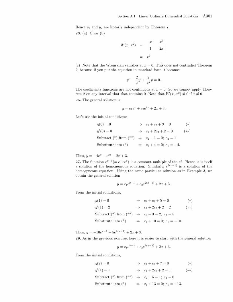
Section A.1 Linear Ordinary Differential Equations A301
Hence y1 and y2 are linearly independent by Theorem 7.
23. (a) Clear (b)
W (x, x2) =
∣∣∣∣∣x x2
1 2x
∣∣∣∣∣
= x2
(c) Note that the Wronskian vanishes at x = 0. This does not contradict Theorem2, because if you put the equation in standard form it becomes
y′′ − 2
xy′ +
2
x2y = 0.
The coefficients functions are not continuous at x = 0. So we cannot apply Theo-rem 2 on any interval that that contains 0. Note that W (x, x2) 6= 0 if x 6= 0.
25. The general solution is
y = c1ex + c2e
2x + 2x+ 3.
Let’s use the initial conditions:
y(0) = 0 ⇒ c1 + c2 + 3 = 0 (∗)y′(0) = 0 ⇒ c1 + 2c2 + 2 = 0 (∗∗)Subtract (*) from (**) ⇒ c2 − 1 = 0; c2 = 1
Substitute into (*) ⇒ c1 + 4 = 0; c1 = −4.
Thus, y = −4ex + e2x + 2x+ 3.
27. The function ex−1(= e−1ex) is a constant multiple of the ex. Hence it is itselfa solution of the homogeneous equation. Similarly, e2(x−1) is a solution of thehomogeneous equation. Using the same particular solution as in Example 3, weobtain the general solution
y = c1ex−1 + c2e
2(x−1) + 2x+ 3.
From the initial conditions,
y(1) = 0 ⇒ c1 + c2 + 5 = 0 (∗)y′(1) = 2 ⇒ c1 + 2c2 + 2 = 2 (∗∗)Subtract (*) from (**) ⇒ c2 − 3 = 2; c2 = 5
Substitute into (*) ⇒ c1 + 10 = 0; c1 = −10.
Thus, y = −10ex−1 + 5e2(x−1) + 2x+ 3.
29. As in the previous exercise, here it is easier to start with the general solution
y = c1ex−2 + c2e
2(x−2) + 2x+ 3.
From the initial conditions,
y(2) = 0 ⇒ c1 + c2 + 7 = 0 (∗)y′(1) = 1 ⇒ c1 + 2c2 + 2 = 1 (∗∗)Subtract (*) from (**) ⇒ c2 − 5 = 1; c2 = 6
Substitute into (*) ⇒ c1 + 13 = 0; c1 = −13.
A302 Appendix A Ordinary Differential Equations: Review of Concepts and Methods
Thus, y = −13ex−2 + 6e2(x−2) + 2x+ 3.
31. Project Problem: Abel’s formula for n = 3.(a) Let y1, y2, y3 be any three solutions of the third order equation
y′′′ + p2(x)y′′ + p1(x)y
′ + p0(x)y = 0.
Then the Wronskian is (expand along the 3rd row):
W (y1, y2, y3) =
∣∣∣∣∣∣∣∣
y1 y2 y3
y′1 y′2 y′3
y′′1 y′′1 y′′3
∣∣∣∣∣∣∣∣
= y′′1
∣∣∣∣∣y2 y3
y′2 y′3
∣∣∣∣∣− y′′2
∣∣∣∣∣y1 y3
y′1 y′3
∣∣∣∣∣
+y′′3
∣∣∣∣∣y1 y2
y′1 y′2
∣∣∣∣∣
= (y2y′3 − y′2y3)y
′′1 − (y1y
′3 − y′1y3)y
′′2
+(y1y′2 − y′1y2)y
′′3 .
Using the product rule to differentiate W , we find
W ′(y1 , y2, y3) = (y2y′3 − y′2y3)y
′′′1 + (y′2y
′3 + y2y
′′3 − y′′2 y3 − y′2y
′3)y
′′1
−(y1y′3 − y′1y3)y
′′′2 − (y′1y
′3 + y1y
′′3 − y′′1 y3 − y′1y
′3)y
′′2
+(y1y′2 − y′1y2)y
′′′3 + (y′1y
′2 + y1y
′′2 − y′′1 y2 − y′1y
′2)y
′′3
= (y2y′3 − y′2y3)y
′′′1 − (y1y
′3 − y′1y3)y
′′′2 + (y1y
′2 − y′1y2)y
′′′3 .
(b) For each j = 1, 2, 3, we have, from the differential equation,
y′′′j = −p2(x)y′′j − p1(x)y
′j − p0(x)yj .
Substituting this into the formula for W ′, we obtain
W ′ = −(y2y′3 − y′2y3)
(p2(x)y
′′1 + p1(x)y
′1 + p0(x)y1
)
+(y1y′3 − y′1y3)
(p2(x)y
′′2 + p1(x)y
′2 + p0(x)y2
)
−(y1y′2 − y′1y2)
(p2(x)y
′′3 + p1(x)y
′3 + p0(x)y3
)
= −p2(x)(y2y′3 − y′2y3)y
′′1 + p2(x)(y1y
′3 − y′1y3)y
′′2
−p2(x)(y1y′2 − y′1y2)y
′′3
= −p2(x)W.
(c) From (b) W satisfies a the first order differential equation W ′ = −p2W , whosesolution is
W = Ce−R
p2(x)dx.
32. (a) Let f(x) = |x3|,
f(x) =
x3 if x > 0
0 if x = 0
−x3 if x < 0
Section A.1 Linear Ordinary Differential Equations A303
Clearly f ′(x) exists if x 6=. For x = 0, we have
f ′(0) = limh→
f(x + h) − f(x)
h
= limh→
|h|3h
= limh→
h2|h|h
= limh→
h|h| = 0.
Hence the derivative exists for all x and is given by
f ′(x) =
3x2 if x > 0
0 if x = 0
−3x2 if x < 0
Another way of writing the derivative is f ′(x) = 3x2 sgnx, where sgn x = −1, 0, or1, according as x < 0, x = 0, or x > 0. We have
W (x3, |x3|) =
∣∣∣∣∣x3 |x3|3x2 3x2 sgnx
∣∣∣∣∣
= 3x5 sgnx− 3x2|x3|.
You can easily verify that the last expression is identically 0 by considering thecases x > 0, x = 0, and x < 0 separately.(b) The functions x3 and |x3| are linearly independent on the real line because oneis not a constant multiple of the other.(c) This does not contradict Theorem 7 because x3 and |x3| are not solution of adifferential equation of the form (3).
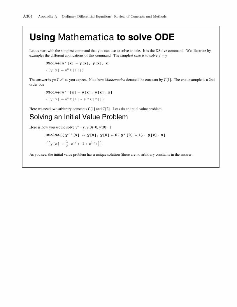
A304 Appendix A Ordinary Differential Equations: Review of Concepts and Methods
Using to solve ODE
Let us start with the simplest command that you can use to solve an ode. It is the DSolve command. We illustrate by
examples the different applications of this command. The simplest case is to solve y' = y
DSolve y’ x y x , y x , x
y x x C 1
The answer is y= C ex as you expect. Note how Mathematica denoted the constant by C[1]. The enxt example is a 2nd
order ode
DSolve y’’ x y x , y x , x
y x x C 1 x C 2
Here we need two arbitrary constants C[1] and C[2]. Let's do an intial value problem.
Solving an Initial Value Problem
Here is how you would solve y'' = y, y(0)=0, y'(0)= 1
DSolve y’’ x y x , y 0 0, y’ 0 1 , y x , x
y x1
2x 1 2 x
As you see, the initial value problem has a unique solution (there are no arbitrary constants in the answer.
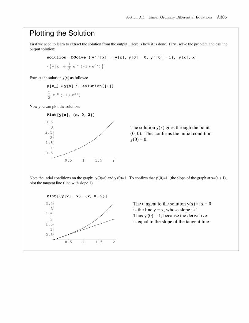
Section A.1 Linear Ordinary Differential Equations A305
Plotting the Solution
First we need to learn to extract the solution from the output. Here is how it is done. First, solve the problem and call the
output solution:
solution DSolve y’’ x y x , y 0 0, y’ 0 1 , y x , x
y x1
2x 1 2 x
Extract the solution y(x) as follows:
y x_ y x . solution 1
1
2x 1 2 x
Now you can plot the solution:
Plot y x , x, 0, 2
0.5 1 1.5 2
0.5
1
1.5
2
2.5
3
3.5
Note the intial conditions on the graph: y(0)=0 and y'(0)=1. To confirm that y'(0)=1 (the slope of the graph at x=0 is 1),
plot the tangent line (line with slope 1)
Plot y x , x , x, 0, 2
0.5 1 1.5 2
0.5
1
1.5
2
2.5
3
3.5
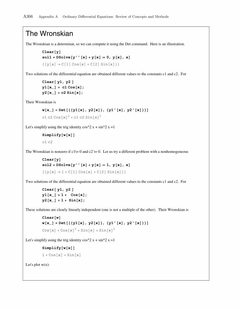
A306 Appendix A Ordinary Differential Equations: Review of Concepts and Methods
The Wronskian
The Wronskian is a determinat, so we can compute it using the Det command. Here is an illustration.
Clear y
sol1 DSolve y’’ x y x 0, y x , x
y x C 1 Cos x C 2 Sin x
Two solutions of the differential equation are obtained different values to the constants c1 and c2. For
Clear y1, y2
y1 x_ c1 Cos x ;
y2 x_ c2 Sin x ;
Their Wronskian is
w x_ Det y1 x , y2 x , y1’ x , y2’ x
c1 c2 Cos x2
c1 c2 Sin x2
Let's simplify using the trig identity cos^2 x + sin^2 x =1
Simplify w x
c1 c2
The Wronskian is nonzero if c1\= 0 and c2 \= 0. Let us try a different problem with a nonhomogeneous
Clear y
sol2 DSolve y’’ x y x 1, y x , x
y x 1 C 1 Cos x C 2 Sin x
Two solutions of the differential equation are obtained different values to the constants c1 and c2. For
Clear y1, y2
y1 x_ 1 Cos x ;
y2 x_ 1 Sin x ;
These solutions are clearly linearly independent (one is not a multiple of the other). Their Wronskian is
Clear w
w x_ Det y1 x , y2 x , y1’ x , y2’ x
Cos x Cos x2
Sin x Sin x2
Let's simplify using the trig identity cos^2 x + sin^2 x =1
Simplify w x
1 Cos x Sin x
Let's plot w(x):
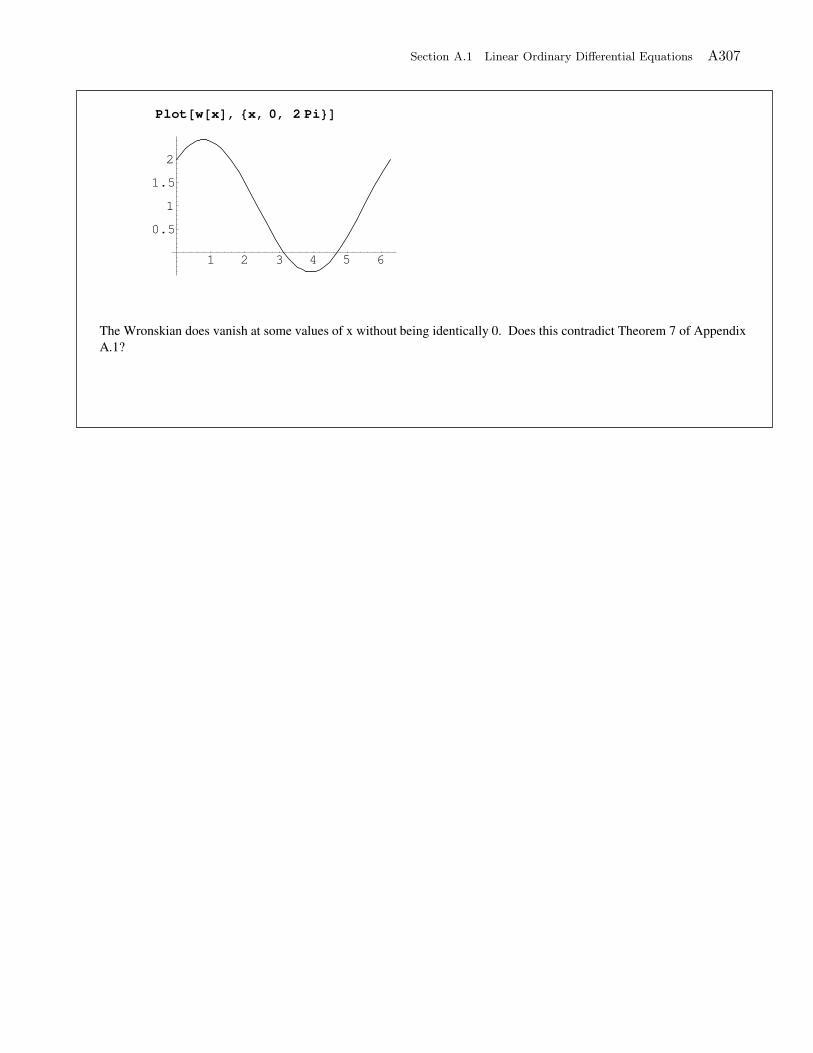
Section A.1 Linear Ordinary Differential Equations A307
Plot w x , x, 0, 2 Pi
1 2 3 4 5 6
0.5
1
1.5
2
The Wronskian does vanish at some values of x without being identically 0. Does this contradict Theorem 7 of Appendix
A.1?
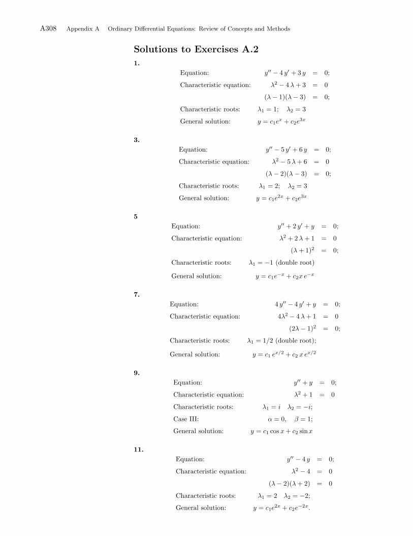
A308 Appendix A Ordinary Differential Equations: Review of Concepts and Methods
Solutions to Exercises A.2
1.
Equation: y′′ − 4 y′ + 3 y = 0;
Characteristic equation: λ2 − 4λ + 3 = 0
(λ− 1)(λ− 3) = 0;
Characteristic roots: λ1 = 1; λ2 = 3
General solution: y = c1ex + c2e
3x
3.
Equation: y′′ − 5 y′ + 6 y = 0;
Characteristic equation: λ2 − 5λ+ 6 = 0
(λ − 2)(λ − 3) = 0;
Characteristic roots: λ1 = 2; λ2 = 3
General solution: y = c1e2x + c2e
3x
5
Equation: y′′ + 2 y′ + y = 0;
Characteristic equation: λ2 + 2λ + 1 = 0
(λ + 1)2 = 0;
Characteristic roots: λ1 = −1 (double root)
General solution: y = c1e−x + c2x e
−x
7.
Equation: 4 y′′ − 4 y′ + y = 0;
Characteristic equation: 4λ2 − 4λ+ 1 = 0
(2λ− 1)2 = 0;
Characteristic roots: λ1 = 1/2 (double root);
General solution: y = c1 ex/2 + c2 x e
x/2
9.
Equation: y′′ + y = 0;
Characteristic equation: λ2 + 1 = 0
Characteristic roots: λ1 = i λ2 = −i;Case III: α = 0, β = 1;
General solution: y = c1 cos x+ c2 sinx
11.
Equation: y′′ − 4 y = 0;
Characteristic equation: λ2 − 4 = 0
(λ− 2)(λ+ 2) = 0
Characteristic roots: λ1 = 2 λ2 = −2;
General solution: y = c1e2x + c2e
−2x.
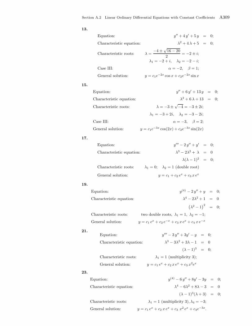
Section A.2 Linear Ordinary Differential Equations with Constant Coefficients A309
13.
Equation: y′′ + 4 y′ + 5 y = 0;
Characteristic equation: λ2 + 4λ + 5 = 0;
Characteristic roots: λ =−4 ±
√16 − 20
2= −2 ± i;
λ1 = −2 + i, λ2 = −2 − i;
Case III: α = −2, β = 1;
General solution: y = c1e−2x cos x+ c2e
−2x sinx
15.
Equation: y′′ + 6 y′ + 13 y = 0;
Characteristic equation: λ2 + 6λ+ 13 = 0;
Characteristic roots: λ = −3 ±√−4 = −3 ± 2i;
λ1 = −3 + 2i, λ2 = −3 − 2i;
Case III: α = −3, β = 2;
General solution: y = c1e−3x cos(2x) + c2e
−3x sin(2x)
17.
Equation: y′′′ − 2 y′′ + y′ = 0;
Characteristic equation: λ3 − 2λ2 + λ = 0
λ(λ − 1)2 = 0;
Characteristic roots: λ1 = 0; λ2 = 1 (double root)
General solution: y = c1 + c2 ex + c3 x e
x
19.
Equation: y(4) − 2 y′′ + y = 0;
Characteristic equation: λ4 − 2λ2 + 1 = 0(λ2 − 1
)2= 0;
Characteristic roots: two double roots, λ1 = 1, λ2 = −1;
General solution: y = c1 ex + c2 e
−x + c3 x ex + c4 x e
−x
21.Equation: y′′′ − 3 y′′ + 3y′ − y = 0;
Characteristic equation: λ3 − 3λ2 + 3λ− 1 = 0
(λ− 1)3 = 0;
Characteristic roots: λ1 = 1 (multiplicity 3);
General solution: y = c1 ex + c2 x e
x + c3 x2ex
23.
Equation: y(4) − 6 y′′ + 8y′ − 3y = 0;
Characteristic equation: λ4 − 6λ2 + 8λ − 3 = 0
(λ − 1)3(λ+ 3) = 0;
Characteristic roots: λ1 = 1 (multiplicity 3), λ4 = −3;
General solution: y = c1 ex + c2 x e
x + c3 x2 ex + c4e
−3x.
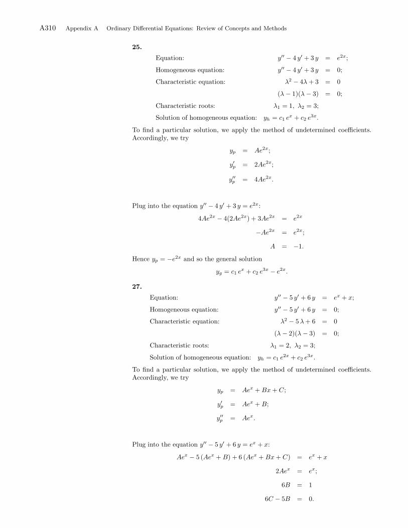
A310 Appendix A Ordinary Differential Equations: Review of Concepts and Methods
25.
Equation: y′′ − 4 y′ + 3 y = e2x;
Homogeneous equation: y′′ − 4 y′ + 3 y = 0;
Characteristic equation: λ2 − 4λ + 3 = 0
(λ − 1)(λ − 3) = 0;
Characteristic roots: λ1 = 1, λ2 = 3;
Solution of homogeneous equation: yh = c1 ex + c2 e
3x.
To find a particular solution, we apply the method of undetermined coefficients.Accordingly, we try
yp = Ae2x;
y′p = 2Ae2x;
y′′p = 4Ae2x.
Plug into the equation y′′ − 4 y′ + 3 y = e2x:
4Ae2x − 4(2Ae2x) + 3Ae2x = e2x
−Ae2x = e2x;
A = −1.
Hence yp = −e2x and so the general solution
yg = c1 ex + c2 e
3x − e2x.
27.
Equation: y′′ − 5 y′ + 6 y = ex + x;
Homogeneous equation: y′′ − 5 y′ + 6 y = 0;
Characteristic equation: λ2 − 5λ+ 6 = 0
(λ − 2)(λ − 3) = 0;
Characteristic roots: λ1 = 2, λ2 = 3;
Solution of homogeneous equation: yh = c1 e2x + c2 e
3x.
To find a particular solution, we apply the method of undetermined coefficients.Accordingly, we try
yp = Aex + Bx+ C;
y′p = Aex + B;
y′′p = Aex.
Plug into the equation y′′ − 5 y′ + 6 y = ex + x:
Aex − 5 (Aex + B) + 6 (Aex + Bx+ C) = ex + x
2Aex = ex;
6B = 1
6C − 5B = 0.
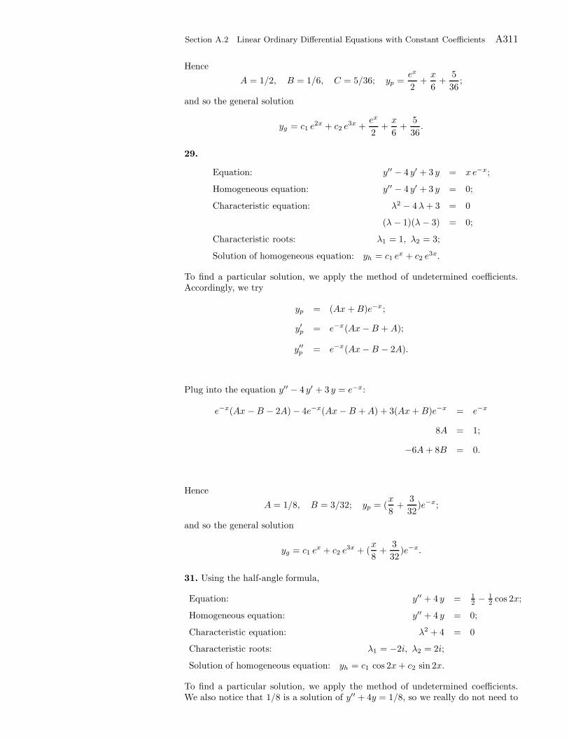
Section A.2 Linear Ordinary Differential Equations with Constant Coefficients A311
Hence
A = 1/2, B = 1/6, C = 5/36; yp =ex
2+x
6+
5
36;
and so the general solution
yg = c1 e2x + c2 e
3x +ex
2+x
6+
5
36.
29.
Equation: y′′ − 4 y′ + 3 y = x e−x;
Homogeneous equation: y′′ − 4 y′ + 3 y = 0;
Characteristic equation: λ2 − 4λ+ 3 = 0
(λ − 1)(λ − 3) = 0;
Characteristic roots: λ1 = 1, λ2 = 3;
Solution of homogeneous equation: yh = c1 ex + c2 e
3x.
To find a particular solution, we apply the method of undetermined coefficients.Accordingly, we try
yp = (Ax +B)e−x;
y′p = e−x(Ax−B + A);
y′′p = e−x(Ax−B − 2A).
Plug into the equation y′′ − 4 y′ + 3 y = e−x:
e−x(Ax −B − 2A) − 4e−x(Ax− B +A) + 3(Ax+ B)e−x = e−x
8A = 1;
−6A + 8B = 0.
Hence
A = 1/8, B = 3/32; yp = (x
8+
3
32)e−x;
and so the general solution
yg = c1 ex + c2 e
3x + (x
8+
3
32)e−x.
31. Using the half-angle formula,
Equation: y′′ + 4 y = 12 − 1
2 cos 2x;
Homogeneous equation: y′′ + 4 y = 0;
Characteristic equation: λ2 + 4 = 0
Characteristic roots: λ1 = −2i, λ2 = 2i;
Solution of homogeneous equation: yh = c1 cos 2x+ c2 sin 2x.
To find a particular solution, we apply the method of undetermined coefficients.We also notice that 1/8 is a solution of y′′ + 4y = 1/8, so we really do not need to
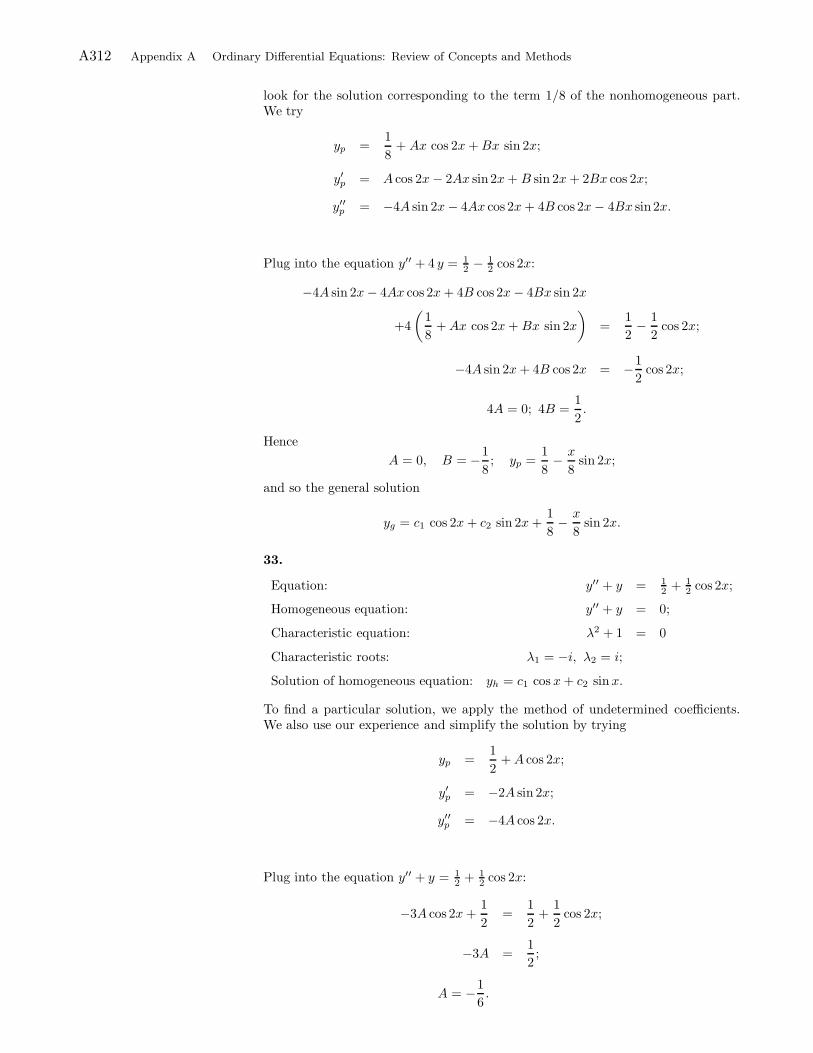
A312 Appendix A Ordinary Differential Equations: Review of Concepts and Methods
look for the solution corresponding to the term 1/8 of the nonhomogeneous part.We try
yp =1
8+ Ax cos 2x+Bx sin 2x;
y′p = A cos 2x− 2Ax sin 2x+ B sin 2x+ 2Bx cos 2x;
y′′p = −4A sin 2x− 4Ax cos 2x+ 4B cos 2x− 4Bx sin 2x.
Plug into the equation y′′ + 4 y = 12 − 1
2 cos 2x:
−4A sin 2x− 4Ax cos 2x+ 4B cos 2x− 4Bx sin 2x
+4
(1
8+Ax cos 2x+ Bx sin 2x
)=
1
2− 1
2cos 2x;
−4A sin 2x+ 4B cos 2x = −1
2cos 2x;
4A = 0; 4B =1
2.
Hence
A = 0, B = −1
8; yp =
1
8− x
8sin 2x;
and so the general solution
yg = c1 cos 2x+ c2 sin 2x+1
8− x
8sin 2x.
33.
Equation: y′′ + y = 12 + 1
2 cos 2x;
Homogeneous equation: y′′ + y = 0;
Characteristic equation: λ2 + 1 = 0
Characteristic roots: λ1 = −i, λ2 = i;
Solution of homogeneous equation: yh = c1 cos x+ c2 sinx.
To find a particular solution, we apply the method of undetermined coefficients.We also use our experience and simplify the solution by trying
yp =1
2+A cos 2x;
y′p = −2A sin 2x;
y′′p = −4A cos 2x.
Plug into the equation y′′ + y = 12 + 1
2 cos 2x:
−3A cos 2x+1
2=
1
2+
1
2cos 2x;
−3A =1
2;
A = −1
6.
Section A.2 Linear Ordinary Differential Equations with Constant Coefficients A313
Hence
yp = −1
6cos 2x+
1
2;
and so the general solution
yg = c1 cos 2x+ c2 sin 2x− 1
6cos 2x+
1
2.
35.
Equation: y′′ + 2 y′ + y = e−x;
Homogeneous equation: y′′ + 2 y′ + y = 0;
Characteristic equation: λ2 + 2λ+ 1 = 0
Characteristic roots: λ1 = −1 (double root);
Solution of homogeneous equation: yh = c1 e−x + c2 x e
−x.
To find a particular solution, we apply the method of undetermined coefficients:
yp = Ax2 e−x;
y′p = −Ax2 e−x + 2Ax e−x;
y′′p = Ax2 e−x − 2Ax e−x + 2Ae−x − 2Ax e−x.
Plug into the equation y′′ + 2 y′ + y = e−x:
Ax2 e−x − 2Ax e−x + 2Ae−x − 2Ax e−x
+2(−Ax2 e−x + 2Ax e−x
)+ Ax2 e−x = e−x;
2Ae−x = e−x;
A =1
2.
Hence
yp =1
2x2e−x;
and so the general solution
yg = c1 e−x + c2 xe
−x +1
2x2e−x.
37.
Equation: y′′ − y′ − 2 y = x2 − 4;
Homogeneous equation: y′′ − y′ − 2 y = 0;
Characteristic equation: λ2 − λ− 2 = 0
Characteristic roots: λ1 = −1, λ2 = 2;
Solution of homogeneous equation: yh = c1 e−x + c2 e
2x.
For a particular solution, try
yp = Ax2 + B x+ C;
y′p = 2Ax+B;
y′′p = 2A.
A314 Appendix A Ordinary Differential Equations: Review of Concepts and Methods
Plug into the equation y′′ − y′ − 2 y = x2 − 4:
2A− 2Ax− B − 2Ax2 − 2B x− 2C = x2 − 4;
−2A = 1;
A = −1
2;
−2A− 2B = 0 ⇒ 1 − 2B = 0;
B =1
2;
2A− 2C − B = 4 ⇒ −1
2− 1
2− 2C = 4
C =5
4.
Hence
yp = −1
2x2 +
1
2x+
5
4;
and so the general solution
yg = c1 e−x + c2 e
2x − 1
2x2 +
1
2x+
5
4.
39. Even though the equation is first order and we can use the integration factormethod of the previous section, we will use the method of this section to illustrateanother interesting approach.
Equation: y′ + 2 y = 2 x+ sinx;
Homogeneous equation: y′ + 2 y = 0;
Characteristic equation: λ + 2 = 0
Characteristic root: λ1 = −2;
Solution of homogeneous equation: yh = c1 e−2x.
For a particular solution, try
yp = Ax+B + C cos x+D sinx;
y′p = A− C sinx+D cosx;
Plug into the equation y′ + 2 y = 2x+ sinx:
A −C sinx+D cos x+ 2Ax+ 2B + 2C cos x+ 2D sinx = 2x+ sinx;
2A = 2 ⇒ A = 1;
A + 2B = 0 ⇒ B = −1
2A = −1
2;
2D− C = 1 and D + 2C = 0 ⇒ D =2
5, C = −1
5.
Hence
yp = x− 1
2− 1
5cosx+
2
5sinx;
and so the general solution
yg = c1e−2x + x− 1
2− 1
5cosx+
2
5sinx.
Section A.2 Linear Ordinary Differential Equations with Constant Coefficients A315
41. 2 y′ − y = e2x.
Equation: 2 y′ − y = e2x;
Homogeneous equation: 2 y′ − y = 0;
Characteristic equation: 2λ− 1 = 0
Characteristic root: λ1 =1
2;
Solution of homogeneous equation: yh = c1 ex/2.
For a particular solution, try
yp = Ae2x;
y′p = 2Ae2x;
Plug into the equation 2y′ − y = e2x:
4Ae2x −Ae2x = e2x;
3A = 1 ⇒ A =1
3.
Hence
yp =1
3e2x;
and so the general solution
yg = c1ex/2 +
1
3e2x.
43.
Equation: y′′ + 9y =
6∑
n=1
sinnx
n;
Homogeneous equation: y′′ + 9y = 0;
Characteristic roots: λ1 = 3i, λ2 = −3i;
Solution of homogeneous equation: yh = c1 cos 3x+ c2 sin 3x.
To find a particular solution, we note that the term sin 3x3 , which appears in the
nonhomogeneous term, is part of the homogeneous solution. So for a particularsolution that corresponds to this term, we try y3 = A3x sin 3x + B3x cos 3x. Forthe remaining terms of the nonhomogeneous part, use
6∑
n=1, n 6=3
Bn sinnx.
Thus we try
yp = A3x sin 3x+B3x cos 3x+6∑
n=1, n 6=3
Bn sinnx;
y′p = A3 sin 3x+ 3A3x cos 3x+B3 cos 3x− 3B3x sin 3x+6∑
n=1, n 6=3
nBn cos nx;
y′′p = 3A3 cos 3x+ 3A3 cos 3x− 9A3x sin 3x− 3B3 sin 3x− 3B3 sin 3x
−9B3x cos 3x−6∑
n=1, n 6=3
n2Bn sinnx;
A316 Appendix A Ordinary Differential Equations: Review of Concepts and Methods
Plug into the equation y′′ + 9y = sin 3x3 +
∑6n=1, n 6=3
sin nxn :
6A3 cos 3x− 6B3 sin 3x+
6∑
n=1, n 6=3
(9 − n2)Bn sinnx =sin 3x
3+
6∑
n=1, n 6=3
sinnx
n
6A3 cos 3x− 6B3 sin 3x =sin 3x
3;
6∑
n=1, n 6=3
(9 − n2)Bn sinnx =
6∑
n=1, n 6=3
sinnx
n;
6A3 = 0, −6B3 =1
3⇒ A3 = 0, B3 = − 1
18;
(n2 − 9)Bn =1
n(n 6= 3) ⇒ Bn =
1
n(9 − n2).
Hence
yp = − 1
18x cos 3x+
6∑
n=1, n 6=3
sinnx
n(9 − n2);
and so the general solution
yg = c1 cos 3x+ c2 sin 3x− 1
18x cos 3x+
6∑
n=1, n 6=3
sinnx
n(9 − n2).
45. Write the equation in the form
y′′ − 4 y′ + 3 y = e2x sinhx
= e2x 1
2
(ex − e−x
)
=1
2
(e3x − ex
).
From Exercise 25, yh = c1ex + c2e
3x. For a particular solution try
yp = Axe3x +Bxex.
47. y′′ + 2y′ + 2 y = cos x+ 6x2 − e−x sinx. Characteristic equation
λ2 + 2λ+ 2 = 0 ⇒ λ = −1 ± i.
So yh = c1e−x cosx+ c2e
−x sinx. For a particular solution, try
yp = A cosx+ B sinx+Cx2 +Dx +E + e−x(Fx sinx+Gx cosx
).
49. y′′ − 3 y′ + 2 y = 3x4ex + x e−2x cos 3x. Characteristic equation
λ2 − 3λ+ 2 = 0 ⇒ λ1 = 1, λ2 = 2.
So yh = c1ex + c2e
2x. For a particular solution, try
yp = x(Ax4+Bx3 +Cx2+Dx+E)ex +(Gx+H) e−2x cos 3x+(Kx+L) e−2x sin 3x.
51. y′′ + 4 y = e2x(sin 2x + 2 cos 2x). We have yh = c1 cos 2x + c2 sin 2x. For aparticular solution, try
yp = e2x(A sin 2x+B cos 2x).
Section A.2 Linear Ordinary Differential Equations with Constant Coefficients A317
53. y′′ − 2 y′ + y = 6x− ex. Characteristic equation
λ2 − 2λ+ 1 = 0 ⇒ λ1 = 1(double root).
So yh = c1ex + c2xe
x. For a particular solution, try
yp = Ax+ B +Cx2ex.
55. From Exercise 25, we have
yh = c1ex + c2e
3x.
If α 6= 1 or 3 (the characteristic roots), a particular solution of
y′′ − 4y′ + 3y = eαx
is yp = Aeαx. Plugging into the equation, we find
Aα2eαx − 4αAeαx + 3Aeαx = eαx;
A(α2 − 4α+ 3) = 1 (divide by eαx 6= 0);
A =1
α2 − 4α+ 3.
Note that α2 − 4α+ 3 6= 0, because α 6= 1 or 3. So the general solution in this caseis of the form
yg = c1ex + c2e
3x +eαx
α2 − 4α+ 3.
If α = λ is one of the characteristic roots 1 or 3, then we modify the particularsolution and use yp = Axeλx. Then
y′p = Aeλx +Axλeλx,
y′′p = Aλeλx + Aλeλx + Axλ2eλx
= 2Aλeλx +Axλ2eλx.
Plug into the left side of the equation
2Aλeλx + Axλ2eλx − 4(Aeλx + Axλeλx
)+ 3Axλeλx
= Axeλx
=0︷ ︸︸ ︷(λ2 − 4λ+ 3
)−2Aλeλx
= −2Aλeλx.
This should equal eλx. So −2A = 1 or A = −1/2 and hence
yg = c1ex + c2e
3x − 1
2xeλx.
57. y′′ + 4y = cosωx. We have
yh = c1 cos 2x+ c2 sin 2x.
If ω 6= ±2, a particular solution of
y′′ + 4y = cosωx
is yp = A cosωx. So y′′p = −Aω2 cosωx. Plugging into the equation, we find
A cosωx(4 − ω2) = cosωx;
A(4 − ω2) = 1;
A =1
4 − ω2.
A318 Appendix A Ordinary Differential Equations: Review of Concepts and Methods
Note that 4 − ω2 6= 0, because ω 6= ±2. So the general solution in this case is ofthe form
yg = c1 cos 2x+ c2 sin 2x+cosωx
4 − ω2.
If ω = ±2, then we modify the particular solution and use yp = x(A cosωx +
B sinωx). Then
y′p =(A cosωx +B sinωx
)+ xω
(−A sinωx+ B cosωx
),
y′′p = xω2(−A cosωx− B sinωx
)+ 2ω
(− A sinωx+B cosωx
).
Plug into the left side of the equation
xω2(−A cosωx−B sinωx
)+2ω
(−A sinωx+B cosωx
)+4x
(A cosωx+B sinωx
).
Using ω2 = 4, this becomes
2ω(− A sinωx+ B cosωx
).
This should equal cosωx. So A = 0 and 2ωB = 1 or B = 1/(2ω).
yg = c1 cos 2x+ c2 sin 2x+1
2ωx sinωx (ω = ±2).
Note that if ω = 2 or ω = −2, the solution is
yg = c1 cos 2x+ c2 sin 2x+1
4x sin 2x.
59. We haveyh = c1 cosωx+ c2 sinωx.
If ω 6= ±2, a particular solution of
y′′ + ω2y = sin 2x
is yp = A sin 2x. So y′′p = −4A sin 2x. Plugging into the equation, we find
A sin 2x(−4 + ω2) = sin2;
A(ω2 − 4) = 1;
A =1
ω2 − 4.
Note that ω2 − 4 6= 0, because ω 6= ±2. So the general solution in this case is ofthe form
yg = c1 cosωx+ c2 sinωx+sin 2x
ω2 − 4.
If ω = ±2, then we modify the particular solution and use yp = Ax cos 2x. Then
y′p = A cos 2x− 2Ax sin 2x,
y′′p = −4A sin 2x− 4Ax cos 2x.
Plug into the equation and get
−4A sin 2x = sin 2x.
So −4A = 1 or A = −1/4. The general solution is
yg = c1 cos 3x+ c2 sin 3x− 1
4x cos 2x.
Section A.2 Linear Ordinary Differential Equations with Constant Coefficients A319
61. To solve y′′ − 4 y = 0, y(0) = 0, y′(0) = 3, start with the general solution
y(x) = c1 cosh 2x+ c2 sinh 2x.
Then
y(0) = 0 ⇒ c1 cosh 0 + c2 sinh 0 = 0
⇒ c1 = 0; so y(x) = c2 sinh 2x.
y′(0) = 3 ⇒ 2c2 cosh 0 = 3
⇒ c2 =3
2
⇒ y(x) =3
2sinh 2x.
63. To solve 4y′′ − 4 y′ + y = 0, y(0) = −1, y′(0) = 1, recall the solution of thehomogeneous equation from Exercise 7:
y = c1ex/2 + c2x e
x/2.
Then
y(0) = −1 ⇒ c1 = −1; so y(x) = −ex/2 + c2x ex/2.
y′(0) = 1 ⇒ −1
2+ c2 = 1
⇒ c2 =3
2
⇒ y(x) = −ex/2 +3
2x ex/2.
65. To solve y′′ − 5 y′ + 6 y = ex, y(0) = 0, y′(0) = 0, use the general solutionfrom Exercise 27 (modify it slightly):
y = c1 e2x + c2 e
3x +1
2ex.
Then
y(0) = 0 ⇒ c1 + c2 = −1
2;
y′(0) = 0 ⇒ 2c1 + 3c2 = −1
2
⇒ c2 =1
2; c1 = −1
⇒ y(x) = − e2x +1
2e3x +
1
2ex.
67. Start with the homogeneous equation y′′ − 4 y′ + 3 y = 0. Its characteristicequation is
λ2 − 4λ+ 3 = 0 ⇒ λ1 = 1, λ2 = 3.
Thusyh = c1e
x + c2e3x.
For a particular solution of y′′ − 4 y′ + 3 y = x e−x, try
y = (Ax+ b)e−x, y′ = Ae−x − (Ax+ b)e−x, y′′ = −2Ae−x + (Ax + b)e−x.
A320 Appendix A Ordinary Differential Equations: Review of Concepts and Methods
Plug into the equation and get
−2Ae−x + (Ax + b)e−x − 4(Ae−x − (Ax+ b)e−x) + 3(Ax+ b)e−x = x e−x
e−x(− 2A+ b− 4A+ 4b+ 3b
)+ xe−x
(A+ 4A+ 3A
)= xe−x;
−6A+ 8b = 0
8A = 1;
A =1
8, b =
6
64=
3
32.
So the general solution is
y = c1ex + c2e
3x + (1
8x+
3
32)e−x.
We can now solve y′′ − 4 y′ + 3 y = x e−x, y(0) = 0, y′(0) = 1. The boundaryconditions imply that
c1 + c2 +3
32= 0
c1 + 3c2 +1
8− 3
32= 0;
c1 + c2 = − 3
32
c1 + 3c2 = − 1
32;
c2 =1
32; c1 = −1
8
Hence
y = −1
8ex +
1
32e3x + (
1
8x+
3
32)e−x.
69. Because of the initial conditions, it is more convenient to take
y = c1 cos[2(x− π
2)] + c2 sin[2(x− π
2)]
as a general solution of y′′ + 4y = 0. For a particular solution of y′′ + 4y = cos 2x,we try
y = Ax sin 2x, y′ = A sin 2x+ 2Ax cos 2x, y′′ = 4A cos 2x− 4Ax sin 2x.
Plug into the equation,
4A cos 2x = cos 2x ⇒ A =1
4.
So the general solution is
y = c1 cos[2(x− π
2)] + c2 sin[2(x− π
2)] +
1
4x sin 2x.
Using the initial conditions
y(π/2) = 1 ⇒ c1 = 1
y′(π/2) = 0 ⇒ 2c2 +π
4cosπ = 0
⇒ c2 =π
8;
Section A.2 Linear Ordinary Differential Equations with Constant Coefficients A321
and so
y = cos[2(x− π
2)] +
π
8sin[2(x− π
2)] +
1
4x sin 2x.
using the addition formulas for the cosine and sine, we can write
cos[2(x− π
2)] = − cos 2x and sin[2(x− π
2)] = − sin 2x,
and so
y = − cos 2x− π
8sin 2x+
1
4x sin 2x = − cos 2x+
(− π
8+
1
4x)sin 2x.
71. An antiderivative of g(x) = ex sinx is a solution of the differential equation
y′ = ex sinx.
To solve this equation we used the method of undetermined coefficients. The solu-tion of homogeneous equation y′ = 0 is clearly y = c. To find a particular solutionof y′ = ex sinx we try
y = ex(A sinx+B cosx)
y′ = ex(A sinx+B cosx) + ex(A cos x−B sinx)
= ex(A− B) sinx+ ex(A +B);
Plugging into the equation, we find
ex(A −B) sin x+ ex(A +B) cos x = ex sinx
A− B = 1, A+B = 0 ⇒ A =1
2, B = −1
2;
so ∫ex sinx dx =
1
2ex sinx− 1
2ex cosx+ C =
ex
2
(sinx− cos x
)+C.
73. An antiderivative of g(x) = ea x cos bx is a solution of the differential equation
y′ = ea x cos bx.
We assume throughout this exercise that a 6= 0 and b 6= 0. For these specialcases the integral is clear. To solve the differential equation we used the method ofundetermined coefficients. The solution of homogeneous equation y′ = 0 is y = C.To find a particular solution of y′ = eax cos bx we try
y = eax(A cos bx+B sin bx)
y′ = aeax(A cos bx+B sin bx) + eax(−bA sin bx+ bB cos bx)
= eax(Aa + bB) cos bx+ eax(aB − bA) sin bx.
Plugging into the equation, we find
eax(Aa+ bB) cos bx+ eax(aB − bA) sin bx = eax cos bx
Aa+ bB = 1, aB − bA = 0 ⇒ A =a
a2 + b2, B =
b
a2 + b2;
so ∫eax cos bx dx =
eax
a2 + b2(a cos x+ b sin bx
)+C.
Concerning Exercises 75–78 and for information about the Vandermonde de-terminant, please refer to the book “Applied Linear Algebra,” by P. Olver and C.Shakiban, Prentice Hall, 2006.
A322 Appendix A Ordinary Differential Equations: Review of Concepts and Methods
Solutions to Exercises A.3
1. We apply the reduction of order formula and take all constants of integrationequal to 0.
y′′ + 2 y′ − 3 y = 0, y1 = ex;
p(x) = 2,
∫p(x) dx = 2x, e−
R
p(x) dx = e−2x;
y2 = y1
∫e−
R
p(x) dx
y21
dx = ex
∫e−2x
e2xdx
= ex
∫e−4x dx = ex
[−1
4e−4x
]= −1
4e−3x.
Thus the general solution is
y = c1ex + c2e
−3x.
3. x y′′− (3+x)y′ +3y = 0, y1 = ex. We first put the equation in standard form.
y′′ − 3 + x
xy′ +
3
xy = 0, y1 = ex; p(x) = −3 + x
x,
∫(−3
x− 1) dx = −3 lnx− x,
e−R
p(x)dx = e3 ln x+x = x3ex;
y2 = y1
∫e−
R
p(x) dx
y21
dx = ex
∫x3ex
e2xdx
= ex
∫x3e−x dx
= ex[−x3e−x − 3x2e−x − 6xe−x − 6e−x
]
= −x3 − 3x2 − 6x− 6.
Thus the general solution is
y = c1ex + c2(x
3 + 3x2 + 6x+ 6).
5. y′′ + 4 y = 0, y1 = cos 2x.
y′′ + 4 y = 0, y1 = cos 2x;
p(x) = 0,
∫p(x) dx = 0, e−
R
p(x) dx = 1;
y2 = y1
∫e−
R
p(x) dx
y21
dx = cos 2x
∫1
cos2 2xdx
= cos 2x
∫sec2 2x dx
= cos 2x
[1
2tan 2x
]=
1
2sin 2x.
Section A.3 Linear Ordinary Differential Equations with Nonconstant Coefficients A323
Thus the general solution is
y = c1 cos 2x+ c2 sin 2x.
7.
y′′ − y = 0, y1 = cosh x;
p(x) = 0,
∫p(x) dx = 0, e−
R
p(x)dx = 1;
y2 = y1
∫e−
R
p(x)dx
y21
dx = cosh x
∫1
cosh2 xdx
= cosh x
∫sech 2x dx
= cosh x [tanhx] = sinhx.
Thus the general solution is
y = c1 coshx+ c2 sinhx.
9. Put the equation in standard form:
(1 − x2)y′′ − 2xy′ + 2y = 0, y1 = x;
y′′ − 2x
1 − x2y′ +
2
1 − x2y = 0, p(x) = − 2x
1 − x2;
∫p(x) dx =
∫− 2x
1 − x2dx = ln(1 − x2)
e−R
p(x)dx = e− ln(1−x2) =1
1 − x2;
y2 = x
∫1
(1 − x2)x2dx.
To evaluate the last integral, we use the partial fractions decomposition
1
(1 − x2)x2=
1
(1 − x)(1 + x)x2
=A
(1 − x)+
B
(1 − x)+C
x+D
x2;
=A(1 + x)x2 +B(1 − x)x2 +C(1 − x2)x+D(1 − x2)
(1 − x)(1 + x)x2
1 = A(1 + x)x2 +B(1 − x)x2 +C(1 − x2)x+D(1 − x2).
Take x = 0 ⇒ D = 1.
Take x = 1 ⇒ 1 = 2A, A =1
2.
Take x = −1 ⇒ 1 = 2B, B =1
2.
A324 Appendix A Ordinary Differential Equations: Review of Concepts and Methods
Checking the coefficient of x3, we find C = 0. Thus
1
(1 − x2)x2=
1
2(1 − x)+
1
2(1 + x)+ +
1
x2
∫1
(1 − x2)x2dx = −1
2ln(1 − x) +
1
2ln(1 + x) − 1
x
=1
2ln
(1 + x
1 − x
)− 1
x.
So
y2 = x
[1
2ln
(1 + x
1 − x
)− 1
x
]=x
2ln
(1 + x
1 − x
)− 1.
Hence the general solution
y = c1 x+ c2
[x
2ln
(1 + x
1 − x
)− 1
].
11. Put the equation in standard form:
x2y′′ + xy′ − y = 0, y1 = x;
y′′ +1
xy′ − 1
x2y = 0, p(x) =
1
x;
∫p(x) dx =
∫1
xdx = lnx
e−R
p(x) dx = e− ln x =1
x;
y2 = x
∫1
x3dx
= x
[−1
2x−2
]
=−1
2x.
Hence the general solution
y = c1x+c2x.
13. Put the equation in standard form:
x2y′′ + xy′ + y = 0, y1 = cos(lnx);
y′′ +1
xy′ +
1
x2y = 0, p(x) =
1
x;
∫p(x) dx =
∫1
xdx = lnx
e−R
p(x) dx = e− ln x =1
x;
y2 = cos(lnx)
∫1
x cos2(lnx)dx
= cos(lnx)
∫1
cos2 udu (u = lnx, du =
1
xdx)
= cos u tanu = sinu = sin(lnu).
Section A.3 Linear Ordinary Differential Equations with Nonconstant Coefficients A325
Hence the general solution
y = c1 cos(lnx) + c2 sin(lnu).
15. Put the equation in standard form:
x y′′ + 2 y′ + 4x y = 0, y1 =sin 2x
x;
y′′ +2
xy′ + 4y = 0, p(x) =
2
x;
∫p(x) dx =
∫2
xdx = 2 lnx
e−R
p(x) dx = e−2 ln x =1
x2;
y2 =sin 2x
x
∫x2
x2 sin2(2x)dx
=sin 2x
x
∫1
sin2(2x)dx =
sin 2x
x
1
−2cot(2x)
=cos 2x
−2x.
Hence the general solution
y = c1sin 2x
x+ c2
cos 2x
x.
17. Put the equation in standard form:
x y′′ + 2 (1 − x)y′ + (x− 2) y = 0, y1 = ex;
y′′ +2(1− x)
xy′ +
x− 2
xy = 0, p(x) =
2
x− 2;
∫p(x) dx = 2 lnx− 2x
e−R
p(x)dx = e−2 ln x+2x =e2x
x2;
y2 = ex
∫e2x
x2e2xdx
= ex
∫1
x2dx = −e
x
x.
Hence the general solution
y = c1ex + c2
ex
x.
A326 Appendix A Ordinary Differential Equations: Review of Concepts and Methods
19. Put the equation in standard form:
x2y′′ − 2x y′ + 2 y = 0, y1 = x2;
y′′ − 2
xy′ +
2
x2y = 0, p(x) = −2
x;
∫p(x) dx = −2 lnx
e−R
p(x)dx = e2 ln x = x2;
y2 = x2
∫x2
x4dx
= x2
∫1
x2dx = −x.
Hence the general solutiony = c1x
2 + c2x.
21. y′′ − 4y′ + 3 y = e−x.
λ2 − 4λ + 3 = 0 ⇒ (λ − 1)(λ− 3) = 0
⇒ λ = 1 or λ = 3.
Linearly independent solutions of the homogeneous equation:
y1 = ex and y2 = e3x.
Wronskian:
W (x) =
∣∣∣∣∣ex e3x
ex 3e3x
∣∣∣∣∣ = 3e4x − e4x = 2e4x.
We now apply the variation of parameters formula with
g(x) = e−x;
yp = y1
∫ −y2g(x)W (x)
dx+ y2
∫y1g(x)
W (x)dx
= ex
∫ −e3xe−x
2e4xdx+ e3x
∫exe−x
2e4xdx
= −ex
2
∫e−2x dx+
e3x
2
∫e−4x dx
=ex
4e−2x − e3x
8e−4x =
e−x
4− e−x
8
=e−x
8.
Thus the general solution is
y = c1ex + c2e
3x +e−x
8.
23. 3 y′′ + 13 y′ + 10 y = sinx.
3λ2 + 13λ+ 10 = 0 ⇒ λ =−13 ±
√169 − 120
6=
−13 ± 7
6
⇒ λ = −20
6= −10
3or λ = −1.
Section A.3 Linear Ordinary Differential Equations with Nonconstant Coefficients A327
Two linearly independent solutions of the homogeneous equation:
y1 = e−103 x and y2 = e−x.
Wronskian:
W (x) =
∣∣∣∣∣e−
103 x e−x
−103 e
− 103 x −e−x
∣∣∣∣∣ = −e− 133 x +
10
3e−
133 x =
7
3e−
133 x.
We now apply the variation of parameters formula with
g(x) =sinx
3;
yp = y1
∫ −y2g(x)W (x)
dx+ y2
∫y1g(x)
W (x)dx
= e−103 x
∫ −e−x sinx
3 73e−
133 x
dx+ e−x
∫e−
103 x sinx
3 73e−
133 x
dx
= −1
7e−
103 x
∫e
103 x sinx dx+
1
7e−x
∫ex sinx dx.
Evaluate the integrals with the help of the formulas in the table at the end of thebook and get
yp = −1
7e−
103 x e
103 x
(103 )2 + 12
(10
3sinx− cos x
)+
1
7e−x ex
12 + 12(sinx− cos x)
= −1
7
11009
+ 1
(10
3sinx− cosx
)+
1
7
1
2(sinx− cos x)
= − 9
763
(10
3sinx− cos x
)+
1
14(sinx− cosx)
=7
218sinx− 13
218cos x
Thus the general solution is
y = c1e− 10
3 x + c2e−x +
7
218sinx− 13
218cosx.
25. y′′ + y = sec x.Two linearly independent solutions of the homogeneous equation are:
y1 = cosx and y2 = sinx.
Wronskian:
W (x) =
∣∣∣∣∣cosx sinx
− sinx cosx
∣∣∣∣∣ = 1.
We now apply the variation of parameters formula with
g(x) = sec x =1
cos x;
yp = y1
∫ −y2g(x)W (x)
dx+ y2
∫y1g(x)
W (x)dx
= − cos x
∫sinx
cosxdx+ sinx
∫dx
= cos x · ln (| cosx|) + x sinx.
A328 Appendix A Ordinary Differential Equations: Review of Concepts and Methods
Thus the general solution is
y = c1 cos x+ c2 sinx+ cos x · ln (| cosx|) + x sinx.
27. x y′′ − (1 + x)y′ + y = x3.
Two linearly independent solutions of the homogeneous equation are given:
y1 = 1 + x and y2 = ex.
Wronskian:
W (x) =
∣∣∣∣∣1 + x ex
1 exx
∣∣∣∣∣ = ex + xex − xex = xex.
We now apply the variation of parameters formula with
g(x) =x3
x= x2;
yp = y1
∫ −y2g(x)W (x)
dx+ y2
∫y1g(x)
W (x)dx
= −(1 + x)
∫ex
xexx2 dx+ ex
∫(1 + x)xe−x dx
= −(1 + x)x2
2+ ex
∫(xe−x + x2e−x) dx
= −x3
2− x2
2+ ex
[−xe−x − e−x − x2e−x − 2xe−x − 2e−x
]
= −x3
2− 3
2x2 − 3x− 3.
Thus the general solution is
y = c1(1 + x) + c2ex − x3
2− 3
2x2 − 3x− 3.
This can also be written as
y = c1(1 + x) + c2ex − x3
2− 3
2x2.
29. x2y′′ + 3 xy′ + y =√x. The homogeneous equation is an Euler equation. The
indicial equation is
r2 + 2r + 1 = 0 ⇒ (r + 1)2 = 0.
We have one double indicial root r = −1. Hence the solutions of the homogenousequation
y1 = x−1 and y2 = x−1 lnx.
Wronskian:
W (x) =
∣∣∣∣∣
1x
1x lnx
−1x2
1−ln xx2
∣∣∣∣∣ =1 − lnx
x3+
lnx
x3=
1
x3.
Section A.3 Linear Ordinary Differential Equations with Nonconstant Coefficients A329
We now apply the variation of parameters formula with
g(x) =
√x
x2= x−
32 ;
yp = y1
∫ −y2g(x)W (x)
dx+ y2
∫y1g(x)
W (x)dx
= −1
x
∫lnx
xx3x−
32 dx+
lnx
x
∫1
xx3x−
32 dx
= −1
x
∫ u︷︸︸︷lnx
dv︷ ︸︸ ︷√xdx+
lnx
x
∫x
12 dx
= −1
x
[2
3x3/2 lnx−
∫2
3x3/2 1
xdx
]+
lnx
x
2
3x3/2
=1
x
2
3
2
3x3/2 =
4
9x1/2.
Thus the general solution is
y = c1x−1 + c2x
−1 lnx+4
9x1/2.
31. x2y′′ + 4xy′ + 2 y = 0. Euler equation with α = 4, β = 2, indicial equation
r2 + 3r + 2 = 0 (r + 1)(r + 2) = 0;
indicial roots: r1 = −1, r2 = −2; hence the general solution
y = c1x−1 + c2x
−2.
33. x2y′′ + 3xy′ + y = 0. See Exercise 29.
35. x2y′′ + xy′ + 4y = 0. Euler equation with α = 1, β = 4, indicial equationr2 + 4 = 0; indicial roots: r1 = −2i, r2 = 2i; hence the general solution
y = c1 cos(2 lnx) + c2 sin(2 lnx).
37. x2y′′ + 7xy′ + 13 y = 0. Euler equation with α = 7, β = 13, indicial equationr2 + 6 r + 13 = 0; indicial roots:
r = −3 ±√−4; r1 = −3 − 2i, r2 = −3 + 2i.
Hence the general solution
y = x−3 [c1 cos(2 lnx) + c2 sin(2 lnx)] .
39. (x − 2)2y′′ + 3(x − 2)y′ + y = 0, (x > 2). Let t = x − 2, x = t + 2, y(x) =y(t + 2) = Y (t),
y′ =dy
dx=dY
dx=dY
dt
dt
dx=dY
dt= Y ′;
y′′ =d
dx
(dy
dx
)=
d
dxY ′ ==
dY ′
dt
dt
dx=d2Y
dt2= Y ′′.
The equation becomes t2Y ′′ + 3tY ′ + Y = 0, t > 0. Euler equation with α = 3,β = 1, indicial equation
r2 + 2 r + 1 = 0 (r + 1)2 = 0;
A330 Appendix A Ordinary Differential Equations: Review of Concepts and Methods
one double indicial root r = −1. Hence the general solution
Y = c1t−1 + c2t
−1 ln t,
and soy = c1(x− 2)−1 + c2(x − 2)−1 ln(x− 2).
41. We have
y2 = y1
∫e−
R
p(x) dx
y21
dx.
Using the product rule for differentiation
y′2 = y′1
∫e−
R
p(x)dx
y21
dx+ y1e−
R
p(x) dx
y21
= y′1
∫e−
R
p(x)dx
y21
dx+e−
R
p(x) dx
y1.
So
W (y1, y2) =
∣∣∣∣∣∣
y1 y1∫
e−R
p(x) dx
y21
dx
y′1 y′1∫
e−R
p(x) dx
y21
dx+ e−R
p(x) dx
y1
∣∣∣∣∣∣
= y1y′1
∫e−
R
p(x) dx
y21
dx+ e−R
p(x)dx − y′1y1
∫e−
R
p(x) dx
y21
dx
= e−R
p(x)dx > 0.
This also follows from Abel’s formula, (4), Section A.1.
43 In the equation x2y′′ + αy′ + βy = 0, let t = lnx, x = et, y(x) = y(et) = Y (t).Then,
dt
dx=
1
x= e−t;
y′ =dy
dx=dY
dx=dY
dt
dt
dx= Y ′ · 1
x= Y ′ · e−t;
y′′ =d
dx
[Y ′ · e−t
]= e−t d
dx[Y ′] + Y ′ d
dx[e−t]
= e−t dY′
dt
dt
dx+ Y ′[−e−t dt
dx]
= e−2tY ′′ − e−2tY ′.
Substituting into the equation and simplifying and using x = et, x2 = e2t, weobtain
d2Y
dt2+ (α− 1)
dY
dt+ βY = 0,
which is a second order linear differential equation in Y with constant coefficients.
45. (a) From Abel’s formula (Theorem 2, Section A.1), the Wronskian is
y1y′2 − y′1y2 = Ce− ∫ p(x) dx,
where y1 and y2 are any two solution of (2).(b) Given y1, set C = 1 in (a)
y1y′2 − y′1y2 = e− ∫ p(x)dx.
Section A.3 Linear Ordinary Differential Equations with Nonconstant Coefficients A331
This is a first-order differential equation in y2 that we rewrite as
y′2 −y′1y1y2 = e− ∫ p(x) dx.
The integrating factor is
eR
− y′1
y1dx = e− ln y1 =
1
y1.
Multiply by the integrating factor:
y′2y1
− y′1y21
y2 =1
y1e− ∫ p(x) dx
ord
dx
[y2y1
]=
1
y1e− ∫ p(x) dx
Integrating both sides, we get
y2y1
=
∫ [1
y1e− ∫ p(x)dx
]dx;
y2 = y1
∫ [1
y1e− ∫ p(x) dx
]dx,
which implies (3).
47. In solving the equation y′′ − 4y′ + 3y = ex, y1 = ex, we follow the steps inthe proof of the previous exercise. Let
y1 = ex, y2 = vex, y′2 = v′ex + vex, y′′2 = v′′ex + 2v′ex + vex.
Then
y′′ − 4y′ + 3y = ex ⇒ v′′ex + 2v′ex + vex − 4(v′ex + vex) + 3vex = ex
⇒ v′′ + 2v′ + v − 4(v′ + v) + 3v = 1 (divide by ex)
⇒ v′′ − 2v′ = 1.
As expected, we arrive at a first order o.d.e. in v′. Its solution (using an integratingfactor) is
e−2xv′′ − 2e−2xv′ = e−2x
d
dx
[e−2xv′
]= e−2x
e−2xv′ =
∫e−2x dx =
−1
2e−2x + C
v′ =−1
2+C e2x.
Integrating once more,
v =−x2
+C1 e2x + C2
y2 = vy1 =−x2ex +C1 e
3x +C2ex.
Note that the term C2ex is corresponds to the solution y1.
A332 Appendix A Ordinary Differential Equations: Review of Concepts and Methods
49. 3 y′′ + 13 y′ + 10 y = sinx, y1 = e−x.As in the previous exercise, let
y1 = e−x, y = ve−x, y′ = v′e−x − ve−x, y′′ = v′′e−x − 2v′e−x + ve−x.
Then
3 y′′ + 13 y′ + 10 y = sinx ⇒ 3(v′′e−x − 2v′e−x + ve−x)
+13(v′e−x − ve−x) + 10ve−x = sinx
⇒ 3v′′ + 7v′ = ex sinx
⇒ v′′ +7
3v′ =
1
3ex sinx.
We now solve the first order o.d.e. in v′:
e7x/3v′′ +7
3e7x/3v′ = e7x/3 1
3ex sinx
d
dx
[e7x/3v′
]=
1
3e10x/3 sinx
e7x/3v′ =1
3
∫1
3e10x/3 sinx dx
=1
3
e10x/3
(103
)2 + 1(10
3sinx− cos) +C
v′ =ex
109(10 sinx− 9
3cos) +C.
(We used the table of integrals to evaluate the preceding integral. We will use itagain below.) Integrating once more,
v =10
109
∫ex sinx dx− 9
327
∫ex cosx dx
=10
109
ex
2(sinx− cos x) − 9
327
ex
2(cos x+ sinx) + C
y = vy1 =10
218(sinx− cos x) − 9
654(cosx+ sinx) +Ce−x
= − 13
218cos x+
7
218sinx+Ce−x.
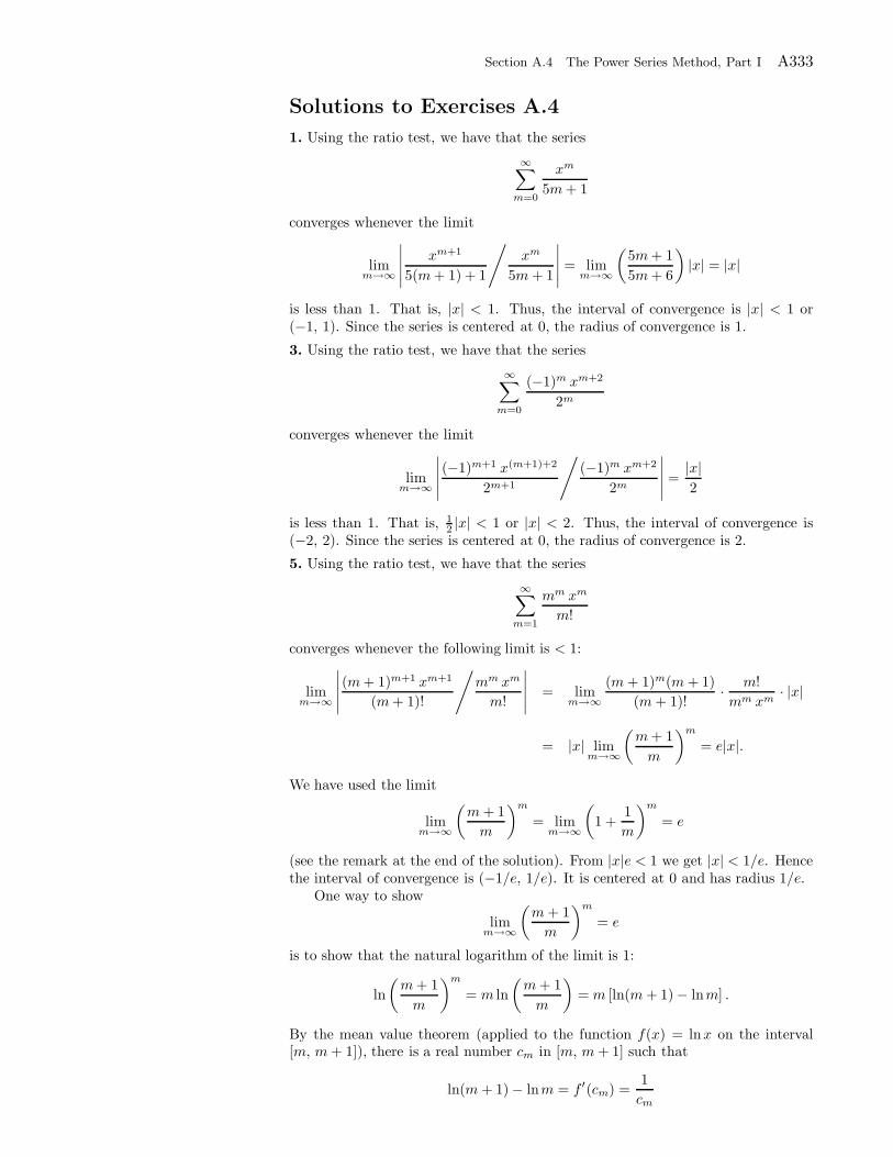
Section A.4 The Power Series Method, Part I A333
Solutions to Exercises A.4
1. Using the ratio test, we have that the series
∞∑
m=0
xm
5m+ 1
converges whenever the limit
limm→∞
∣∣∣∣∣xm+1
5(m+ 1) + 1
/xm
5m+ 1
∣∣∣∣∣ = limm→∞
(5m+ 1
5m+ 6
)|x| = |x|
is less than 1. That is, |x| < 1. Thus, the interval of convergence is |x| < 1 or(−1, 1). Since the series is centered at 0, the radius of convergence is 1.
3. Using the ratio test, we have that the series
∞∑
m=0
(−1)m xm+2
2m
converges whenever the limit
limm→∞
∣∣∣∣∣(−1)m+1 x(m+1)+2
2m+1
/(−1)m xm+2
2m
∣∣∣∣∣ =|x|2
is less than 1. That is, 12 |x| < 1 or |x| < 2. Thus, the interval of convergence is
(−2, 2). Since the series is centered at 0, the radius of convergence is 2.
5. Using the ratio test, we have that the series
∞∑
m=1
mm xm
m!
converges whenever the following limit is < 1:
limm→∞
∣∣∣∣∣(m+ 1)m+1 xm+1
(m+ 1)!
/mm xm
m!
∣∣∣∣∣ = limm→∞
(m+ 1)m(m+ 1)
(m+ 1)!· m!
mm xm· |x|
= |x| limm→∞
(m+ 1
m
)m
= e|x|.
We have used the limit
limm→∞
(m+ 1
m
)m
= limm→∞
(1 +
1
m
)m
= e
(see the remark at the end of the solution). From |x|e < 1 we get |x| < 1/e. Hencethe interval of convergence is (−1/e, 1/e). It is centered at 0 and has radius 1/e.
One way to show
limm→∞
(m+ 1
m
)m
= e
is to show that the natural logarithm of the limit is 1:
ln
(m+ 1
m
)m
= m ln
(m+ 1
m
)= m [ln(m+ 1) − lnm] .
By the mean value theorem (applied to the function f(x) = lnx on the interval[m, m+ 1]), there is a real number cm in [m, m+ 1] such that
ln(m+ 1) − lnm = f ′(cm) =1
cm
A334 Appendix A Ordinary Differential Equations: Review of Concepts and Methods
Note that1
m+ 1≤ 1
cm≤ 1
m.
Som
m+ 1≤ m [ln(m+ 1) − lnm] ≤ 1.
As m→ ∞, mm+1 → 1, and so by the sandwich theorem,
m [ln(m+ 1) − lnm] → 1.
Taking the exponential, we derive the desired limit.
7. Using the ratio test, we have that the series
∞∑
m=2
xm
lnm
converges whenever the limit
limm→∞
∣∣∣∣∣xm+1
ln(m+ 1)
/xm
lnm
∣∣∣∣∣ = |x| limm→∞
lnm
ln(m+ 1)= |x|
is less than 1 (see the note at the end of the solution). That is, |x| < 1. Thus theinterval convergence is (−1, 1). It is centered at 0 and has radius 1. To show that
limm→∞
lnm
ln(m+ 1)= 1,
you can use l’Hospital rule. Differentiating numerator and denominator, we obtain
limm→∞
lnm
ln(m+ 1)= lim
m→∞1/m
1/(m+ 1)= lim
m→∞m+ 1
m= 1.
11. Using the ratio test, we have that the series
∞∑
m=0
2m (x − 2)m
10m
converges whenever the following limit is < 1:
limm→∞
∣∣∣∣∣2m+1 (x− 2)m+1
10m+1
/2m (x− 2)m
10m
∣∣∣∣∣ =2
10|x− 2|.
Thus |x− 2| < 5. Hence the interval of convergence is centered at 2 and has radius5; that is, (−3, 7)
13. We use the geometric series. For |x| < 1,
3 − x
1 + x= −1 + x
1 + x+
4
1 + x
= −1 +4
1 − (−x)
= −1 + 4
∞∑
n=0
(−1)nxn.
15. Start with the geometric series
1
1 − (−x) =
∞∑
n=0
(−1)nxn (|x| < 1).
Section A.4 The Power Series Method, Part I A335
Replace x by x2:
1
1 + x2=
∞∑
n=0
(−1)nx2n (|x2| < 1 or |x| < 1).
Differentiate term-by-term:
−2x
(1 + x2)2=
∞∑
n=1
(−1)n(2n)x2n−1 (|x| < 1).
Divide by −2 both sides,
x
(1 + x2)2=
∞∑
n=1
(−1)n+1nx2n−1 (|x| < 1).
17. Use the Taylor series
ex =
∞∑
n=0
xn
n!−∞ < x <∞.
Then
eu2
=
∞∑
n=0
u2n
n!−∞ < u <∞.
Hence, for all x,
e3x2+1 = e · e(√
3x)2
= e
∞∑
n=0
(√
3x)2n
n!
= e
∞∑
n=0
3nx2n
n!.
19. Using the sine series expansion, we have for all x
x sinx cos x =x
2sin(2x) =
∞∑
n=0
(−1)n (2x)2n+1
(2n+ 1)!=
∞∑
n=0
(−1)n 22n+1
(2n+ 1)!x2n+1.
21.We have1
2 + 3x=
1
2(1 − (−3x2 ))
=1
2(1 − u),
where u = −3x2 . So
1
2 + 3x=
1
2
∞∑
n=0
un =1
2
∞∑
n=0
(−3x
2
)n
=
∞∑
n=0
(−1)n 3n
2n+1xn.
The series converges if |u| < 1; that is |x| < 23 .
23. We have
3x+ x3
2 + 3x2= x
(3x2 + 2 + 1)
3x2 + 2
= x+x
3x2 + 2
= x+x
2(1 − (−32x
2)
= x+x
2(1 − u),
A336 Appendix A Ordinary Differential Equations: Review of Concepts and Methods
where u = −32x
2. So
3x+ x3
2 + 3x2= x+
x
2
∞∑
n=0
un
= x+x
2
∞∑
n=0
(−3
2x2
)n
= x+∞∑
n=0
(−1)n 3n
2n+1x2n+1.
The series converges if |u| < 1; that is x2 < 23 or |x| <
√23 .
25. Let a be any real number 6= 0, then
1
x=
1
a− a+ x
=1
a· 1
1 −(
a−xa
)
=1
a
∞∑
n=0
(a − x
a
)n
=1
a
∞∑
n=0
(−1)n (x− a)n
an.
The series converges if
∣∣∣∣a− x
a
∣∣∣∣ < 1 or |a− x| < |a|.
27. Let f(x) be as in Exercise 26. From the formula for the Taylor coefficients, weknow that
f(x) =
∞∑
n=0
f(n)(0)
n!xn.
Comparing coefficients with
f(x) =∞∑
k=0
(−1)kx2k
(k!)222k,
we find that
f(0) =(−1)0
(0!)220= 1;
f ′(0) = 0;
f ′′(0)
2!=
(−1)1
(1!)222⇒ f ′′(0) = −1
4.
(b) In general, since the Taylor series has no terms with odd powers of x, we findthat find f(2k+1)(0) = 0. For the eve powers, we have
f(2k)(0)
(2k)!=
(−1)k
(k!)222k⇒ f(2k)(0) =
(−1)k(2k)!
(k!)222k.
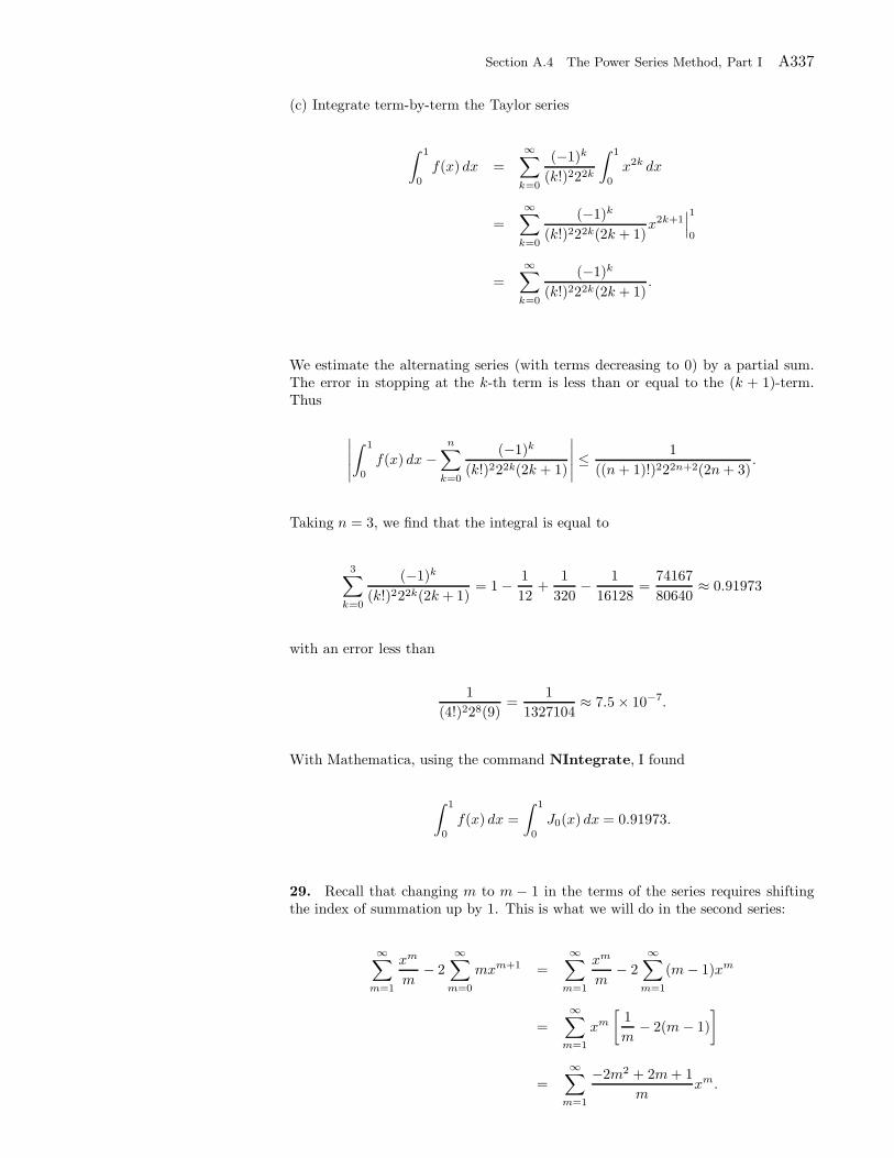
Section A.4 The Power Series Method, Part I A337
(c) Integrate term-by-term the Taylor series
∫ 1
0
f(x) dx =
∞∑
k=0
(−1)k
(k!)222k
∫ 1
0
x2k dx
=
∞∑
k=0
(−1)k
(k!)222k(2k + 1)x2k+1
∣∣∣1
0
=∞∑
k=0
(−1)k
(k!)222k(2k + 1).
We estimate the alternating series (with terms decreasing to 0) by a partial sum.The error in stopping at the k-th term is less than or equal to the (k + 1)-term.Thus
∣∣∣∣∣
∫ 1
0
f(x) dx −n∑
k=0
(−1)k
(k!)222k(2k + 1)
∣∣∣∣∣ ≤1
((n+ 1)!)222n+2(2n+ 3).
Taking n = 3, we find that the integral is equal to
3∑
k=0
(−1)k
(k!)222k(2k + 1)= 1 − 1
12+
1
320− 1
16128=
74167
80640≈ 0.91973
with an error less than
1
(4!)228(9)=
1
1327104≈ 7.5 × 10⁻⁷.
With Mathematica, using the command NIntegrate, I found
∫ 1
0
f(x) dx =
∫ 1
0
J0(x) dx = 0.91973.
29. Recall that changing m to m − 1 in the terms of the series requires shiftingthe index of summation up by 1. This is what we will do in the second series:
∞∑
m=1
xm
m− 2
∞∑
m=0
mxm+1 =
∞∑
m=1
xm
m− 2
∞∑
m=1
(m− 1)xm
=
∞∑
m=1
xm
[1
m− 2(m− 1)
]
=
∞∑
m=1
−2m2 + 2m+ 1
mxm.
A338 Appendix A Ordinary Differential Equations: Review of Concepts and Methods
31.
2x
∞∑
m=2
2√m+ 2xm +
∞∑
m=2
xm−1
m+ 6
=∞∑
m=2
4√m+ 2xm+1 +
∞∑
m=2
xm−1
m+ 6
=
∞∑
m=3
4√m+ 1xm +
∞∑
m=1
xm
m+ 7
=
∞∑
m=3
4√m+ 1xm +
∞∑
m=3
[xm
m+ 7
]+x
8+x2
9
=x
8+x2
9+
∞∑
m=3
[4√m+ 1 +
1
m+ 7
]xm.
33. Let
y =
∞∑
m=0
amxm y′ =
∞∑
m=1
mamxm−1.
Then
y′ + y =
∞∑
m=1
mamxm−1 +
∞∑
m=0
amxm
=
∞∑
m=0
(m+ 1)am+1xm +
∞∑
m=0
amxm
=
∞∑
m=0
[(m+ 1)am+1 + am]xm
35. Let
y =
∞∑
m=0
amxm y′ =
∞∑
m=1
mamxm−1 y′′ =
∞∑
m=2
m(m− 1)amxm−2.
Then
(1 − x2)y′′ + 2xy′ = (1 − x2)
∞∑
m=2
m(m− 1)amxm−2 + 2x
∞∑
m=1
mamxm−1
=
∞∑
m=2
m(m− 1)amxm−2 −
∞∑
m=2
m(m− 1)amxm +
∞∑
m=1
2mamxm
=
∞∑
m=0
(m+ 2)(m+ 1)am+2xm −
∞∑
m=2
m(m− 1)amxm +
∞∑
m=1
2mamxm
= 2a2 + 6a3x+
∞∑
m=2
(m+ 2)(m+ 1)am+2xm
−∞∑
m=2
m(m− 1)amxm + 2a1x+
∞∑
m=2
2mamxm
= 2a2 + (2a1 + 6a3)x
+
∞∑
m=2
[(m+ 2)(m+ 1)am+2 −m(m− 1)am + 2mam]xm.
Section A.4 The Power Series Method, Part I A339
37. Let
y =
∞∑
m=0
amxm y′ =
∞∑
m=1
mamxm−1 y′′ =
∞∑
m=2
m(m− 1)amxm−2.
Then
x2y′′ + y = x2∞∑
m=2
m(m− 1)amxm−2 +
∞∑
m=0
amxm
=
∞∑
m=2
m(m − 1)amxm +
∞∑
m=0
amxm
=
∞∑
m=2
m(m − 1)amxm + a0 + a1x+
∞∑
m=2
amxm
= a0 + a1x+∞∑
m=2
[m(m− 1)am + am] xm
= a0 + a1x+
∞∑
m=2
(m2 −m+ 1)amxm.
39. Let
y =
∞∑
m=0
amxm y′ =
∞∑
m=1
mamxm−1.
Then
xy′ + y − ex =
∞∑
m=1
mamxm +
∞∑
m=0
amxm −
∞∑
m=0
xm
m!
=
∞∑
m=0
mamxm +
∞∑
m=0
amxm −
∞∑
m=0
xm
m!
=
∞∑
m=0
[(m+ 1)am − 1
m!
]xm.
A340 Appendix A Ordinary Differential Equations: Review of Concepts and Methods
Solutions to Exercises A.5
1. For the differential equation y′ + 2xy = 0, p(x) = 1 is its own power seriesexpansion about a = 0. So a = 0 is an ordinary point. To solve, let Let
y =
∞∑
m=0
amxm y′ =
∞∑
m=1
mamxm−1.
Then
y′ + 2xy =
∞∑
m=1
mamxm−1 + 2x
∞∑
m=0
amxm
=∞∑
m=1
mamxm−1 +
∞∑
m=0
2amxm+1
=
∞∑
m=0
(m+ 1)am+1xm +
∞∑
m=1
2am−1xm
= a1 +
∞∑
m=1
[(m+ 1)am+1 + 2am−1]xm.
So y′ + 2xy = 0 implies that
a1 +
∞∑
m=1
[(m+ 1)am+1 + 2am−1] xm = 0;
a1 = 0
(m+ 1)am+1 + 2am−1 = 0
am+1 = − 2
m+ 1am−1.
From the recurrence relation,
a1 = a3 = a5 = · · · = a2k+1 = · · · = 0;
a0 is arbitrary;
a2 = −2
2a0 = −a0,
a4 = −2
4a2 =
1
2!a0,
a6 = −2
6a4 = − 1
3!a0,
a8 = −2
8a6 =
1
4!a0,
...
a2k =(−1)k
k!a0.
So
y = a0
∞∑
k=0
(−1)k
k!x2k = a0
∞∑
k=0
(−x2)k
k!= a0e
−x2
.
Section A.5 The Power Series Method, Part II A341
3. From the previous exercise
y′ + y = x ⇒∞∑
m=0
[(m+ 1)am+1 + am] xm = x
⇒ a1 + a0 = 0 (m = 0)
2a2 + a1 = 1 (m = 1)
(m+ 1)am+1 + am = 0 for all m ≥ 2
⇒ am+1 =am
m+ 1for all m ≥ 2.
So a0 is arbitrary;
a1 = −a0,
a2 =1 + a0
2,
a3 = −1
3a2 = − 1
3!a0 −
1
3!,
a4 = −1
4a3 =
1
4!a0 +
1
4!,
...
am =(−1)m
m!(a0 + 1).
So
y = −1 + x+ (a0 + 1)
∞∑
m=0
(−1)m
m!xm = −1 + x+Ce−x.
5. For the differential equation y′′−y = 0, p(x) = 0 is its own power series expansionabout a = 0. So a = 0 is an ordinary point. To solve, let
y =
∞∑
m=0
amxm y′ =
∞∑
m=1
mamxm−1 y′′ =
∞∑
m=2
m(m− 1)amxm−2.
Then
y′′ − y =
∞∑
m=2
m(m− 1)amxm−2 −
∞∑
m=0
amxm
=
∞∑
m=0
(m+ 2)(m+ 1)am+2xm −
∞∑
m=0
amxm
=
∞∑
m=0
[(m+ 2)(m+ 1)am+2 − am] xm.
So y′′ − y = 0 implies that
(m+ 2)(m+ 1)am+2 − am = 0 ⇒ am+2 =am
(m+ 2)(m+ 1)for all m ≥ 0.
A342 Appendix A Ordinary Differential Equations: Review of Concepts and Methods
So a0 and a1 are arbitrary;
a2 =a0
2,
a4 =a2
4 · 3 =a0
4!,
a6 =a4
6 · 5 =a0
6!,
...
a2n =a0
(2n)!.
.
Similarly,
a2n+1 =a1
(2n+ 1)!,
and so
y = a0
∞∑
n=0
1
(2n)!x2n + a1
∞∑
n=0
1
(2n+ 1)!x2n+1 = a0 coshx+ a1 sinhx.
7. For the differential equation y′′ −x y′ + y = 0, p(x) = −x is its own power seriesexpansion about a = 0. So a = 0 is an ordinary point. To solve, let
y =
∞∑
m=0
amxm y′ =
∞∑
m=1
mamxm−1 y′′ =
∞∑
m=2
m(m− 1)amxm−2.
Then
y′′ − xy′ + y =
∞∑
m=2
m(m− 1)amxm−2 − x
∞∑
m=1
mamxm−1 +
∞∑
m=0
amxm
=
∞∑
m=0
(m+ 2)(m+ 1)am+2xm −
∞∑
m=0
mamxm +
∞∑
m=0
amxm
=
∞∑
m=0
[(m+ 2)(m+ 1)am+2(1 −m)am]xm.
So y′′ − x y′ + y = 0 implies that
(m+2)(m+1)am+2(1−m)am = 0 ⇒ am+2 =(m− 1)
(m+ 2)(m+ 1)am for allm ≥ 0.
So a0 and a1 are arbitrary;
a2 = −a0
2,
a4 =a2
4 · 3 = −a0
4!,
a6 =3a4
6 · 5 = − 3
6!a0,
...
Section A.5 The Power Series Method, Part II A343
Similarly,
a3 = a1 · 0 = 0,
a5 = 0,
...
a2k+1 = 0, k ≥ 1.
So
y = a1x+ a0
(1 − x2
2− x4
4!− 3
6!x6 · · ·
).
9. For the differential equation y′′ +2 x y′ +y = 0, p(x) = 2x is its own power seriesexpansion about a = 0. So a = 0 is an ordinary point. To solve, let
y =
∞∑
m=0
amxm y′ =
∞∑
m=1
mamxm−1 y′′ =
∞∑
m=2
m(m− 1)amxm−2.
Then
y′′ + 2 x y′ + y =
∞∑
m=2
m(m− 1)amxm−2 +
∞∑
m=1
2mamxm +
∞∑
m=0
amxm
=
∞∑
m=0
(m+ 2)(m+ 1)am+2xm +
∞∑
m=0
2mamxm +
∞∑
m=0
amxm
=
∞∑
m=0
[(m+ 2)(m+ 1)am+2 + (2m+ 1)am] xm.
So y′′ + 2 x y′ + y = 0 implies that
(m+ 2)(m+ 1)am+2 + (2m+ 1)am = 0
⇒ am+2 = − (2m+ 1)
(m+ 2)(m+ 1)am for all m ≥ 0.
So a0 and a1 are arbitrary;
a2 = −1
2a0,
a4 = − 5
4 · 3a2 =5
4!a0,
a6 = − 9
6 · 55
4!a0 =
−9 · 56!
a0,
...
a3 = − 3
3 · 2a1
a5 = − 7
5 · 4a3 =7 · 35!
a1
a7 = −11 · 7 · 37!
a1
...
A344 Appendix A Ordinary Differential Equations: Review of Concepts and Methods
So
y = a0
(1 − 1
2x2 +
5
4!x4 − 9 · 5
6!x6 + · · ·
)
+a1
(x− 3
3!x3 +
7 · 35!
x5 − 11 · 7 · 37!
x7 + · · ·).
11. y′′ − 2 y′ + y = 0, y(0) = 0, y′(0) = 1.For the differential equation y′′−2 y′ +y = 0, p(x) = −2 is its own power series
expansion about a = 0. So a = 0 is an ordinary point. To solve, let
y =
∞∑
m=0
amxm y′ =
∞∑
m=1
mamxm−1 y′′ =
∞∑
m=2
m(m− 1)amxm−2.
The initial conditions y(0) = 0, y′(0) = 1 tell us that a0 = 0 and a1 = 1. Then
y′′ − 2 y′ + y =
∞∑
m=2
m(m − 1)amxm−2 − 2
∞∑
m=1
mamxm +
∞∑
m=0
amxm
=
∞∑
m=0
(m+ 2)(m+ 1)am+2xm − 2
∞∑
m=0
(m+ 1)am+1xm +
∞∑
m=0
amxm
=
∞∑
m=0
[(m+ 2)(m+ 1)am+2 − 2(m+ 1)am+1 + am] xm.
So y′′ − 2 y′ + y = 0 implies that
(m+ 2)(m+ 1)am+2 − 2(m+ 1)am+1 + am = 0
⇒ am+2 =2
(m+ 2)am+1 − am
(m+ 2)(m+ 1)for all m ≥ 0.
Using a0 = 0 and a1 = 1, we find
a2 = 1,
a3 =2
3− 1
3 · 2 =1
2,
a4 =1
2
1
2− 1
4 · 3 =1
3!,
...
ak =1
(k − 1)!.
(It is not difficult to derive this formula by induction.) So
y =
∞∑
k=1
1
(k − 1)!xk.
13. To solve (1 − x2)y′′ − 2xy′ + 2y = 0, y(0) = 0, y′(0) = 3, follow the steps inExample 5 and you will arrive at the recurrence relation
am+2 =m(m+ 1) − 2
(m+ 2)(m+ 1)am =
(m+ 2)(m− 1)
(m+ 2)(m+ 1)am =
m− 1
m+ 1am, m ≥ 0.
The initial conditions give you a0 = 0 and a1 = 3. So a2 = a4 = · · · = 0 and, fromthe recurrence relation with m = 1,
a3 =(1 − 1
1 + 1a0 = 0.
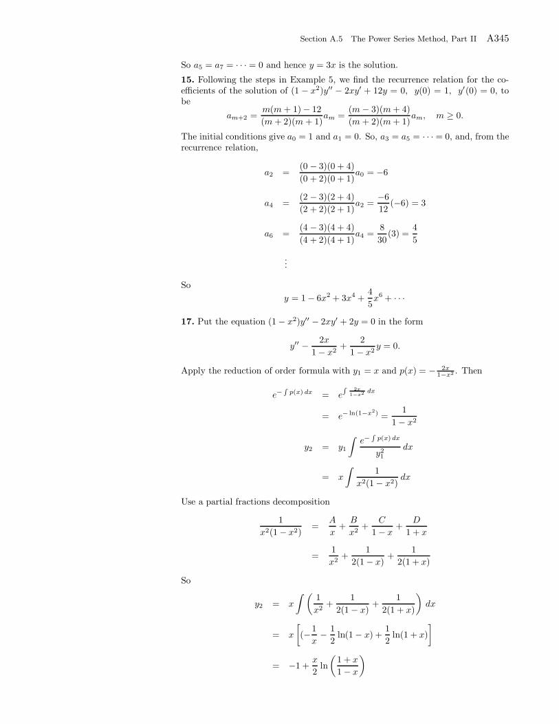
Section A.5 The Power Series Method, Part II A345
So a5 = a7 = · · · = 0 and hence y = 3x is the solution.
15. Following the steps in Example 5, we find the recurrence relation for the co-efficients of the solution of (1 − x2)y′′ − 2xy′ + 12y = 0, y(0) = 1, y′(0) = 0, tobe
am+2 =m(m+ 1) − 12
(m+ 2)(m+ 1)am =
(m− 3)(m+ 4)
(m+ 2)(m+ 1)am, m ≥ 0.
The initial conditions give a0 = 1 and a1 = 0. So, a3 = a5 = · · · = 0, and, from therecurrence relation,
a2 =(0 − 3)(0 + 4)
(0 + 2)(0 + 1)a0 = −6
a4 =(2 − 3)(2 + 4)
(2 + 2)(2 + 1)a2 =
−6
12(−6) = 3
a6 =(4 − 3)(4 + 4)
(4 + 2)(4 + 1)a4 =
8
30(3) =
4
5
...
So
y = 1 − 6x2 + 3x4 +4
5x6 + · · ·
17. Put the equation (1 − x2)y′′ − 2xy′ + 2y = 0 in the form
y′′ − 2x
1 − x2+
2
1 − x2y = 0.
Apply the reduction of order formula with y1 = x and p(x) = − 2x1−x2 . Then
e−R
p(x) dx = eR
2x1−x2 dx
= e− ln(1−x2) =1
1 − x2
y2 = y1
∫e−
R
p(x)dx
y21
dx
= x
∫1
x2(1 − x2)dx
Use a partial fractions decomposition
1
x2(1 − x2)=
A
x+B
x2+
C
1 − x+
D
1 + x
=1
x2+
1
2(1 − x)+
1
2(1 + x)
So
y2 = x
∫ (1
x2+
1
2(1 − x)+
1
2(1 + x)
)dx
= x
[(−1
x− 1
2ln(1 − x) +
1
2ln(1 + x)
]
= −1 +x
2ln
(1 + x
1 − x
)
A346 Appendix A Ordinary Differential Equations: Review of Concepts and Methods
The following notebook illustrates how we can use Mathematica to solve adifferential equations with poser series.
The solution is y and we will solve for the first 10 coefficients.
Let's define a partial sum of the Taylor series solution (degree 3) and set y[0]=1:
In[82]:= seriessol Series y x , x, 0, 3 . y 0 1
Out[82]= 1 y 0 x1
2y 0 x2
1
6y 3 0 x3 O x
4
Next we set equations based on the given differential equation y'+y=0.
In[83]:= leftside D seriessol, x seriessol
rightside 0
equat LogicalExpand leftside rightside
Out[83]= 1 y 0 y 0 y 0 xy 0
2
1
2y 3 0 x2 O x
3
Out[84]= 0
Out[85]= 1 y 0 0 && y 0 y 0 0 &&y 0
2
1
2y 3 0 0
This gives you a set of equations in the coefficients that Mathematica can solve
In[86]:= seriescoeff Solve equat
Out[86]= y 0 1, y 0 1, y 3 0 1
Next, we substitute these coefficients in the series solution. This can be done as follows
In[87]:= seriessol . seriescoeff 1
Out[87]= 1 xx2
2
x3
6O x
4
To get a partial sum without the Big O, use
In[88]:= Normal seriessol . seriescoeff 1
Out[88]= 1 xx2
2
x3
6
Section A.5 The Power Series Method, Part II A347
With the previous example in hand, we can solve Exercises 19-22 using Math-ematica by repeating and modifying the commands. Here is an illustration withExercise 19. We suppress some outcomes to save space.
19. y′′ − y′ + 2y = ex, y(0) = 0, y′(0) = 1.
In[70]:= Clear y, seriessol, n, partsol
n 10
seriessol Series y x , x, 0, n . y 0 0, y’ 0 1
leftside D seriessol, x, 2 D seriessol, x, 1 2 seriessol;
rightside Series E^x, x, 0, n ;
equat LogicalExpand leftside rightside ;
seriescoeff Solve equat ;
partsol Normal seriessol . seriescoeff 1 ;
Out[71]= 10
Out[72]= x1
2y 0 x2
1
6y 3 0 x3
1
24y 4 0 x4
1
120y 5 0 x5
1
720y 6 0 x6
y 7 0 x7
5040
y 8 0 x8
40320
y 9 0 x9
362880
y 10 0 x10
3628800O x
11
The equation can be solved using analytical methods (undetermined coefficients). The exact solution is
sol DSolve y’’ x y’ x 2 y x E^x, y 0 0, y’ 0 1 , y x , x ;
In[46]:= sss sol 1, 1, 2
1
14x 2 7 Cos
7 x
27 x 2 Cos
7 x
2
2
3 7 Sin7 x
27 x 2 Sin
7 x
2
2
Let's compare with the partial sum that we found earlier
In[67]:= Plot sss, partsol , x, 2, 2
-2 -1 1 2
0.5
1
1.5
2
Out[67]= Graphics
We have a nice match on the interval [-2, 2]
A348 Appendix A Ordinary Differential Equations: Review of Concepts and Methods
Solutions to Exercises A.6
1. For the equation y′′ + (1 − x2)y′ + xy = 0, p(x) = 1− x2 and q(x) = x are bothanalytic at a = 0. So a = 0 is a ordinary point.
3. For the equation x3y′′ + x2y′ + y = 0,
p(x) =1
x, x p(x) = 1;
q(x) =2
x3, x2q(x) =
2
x.
p(x) and q(x) are not analytic at 0. So a = 0 is a singular point. Since xp(x)is analytic but x2q(x) is not analytic at a = 0, the point a = 0 is not a regularsingular point.
5. For the equation x2y′′ + (1 − ex)y′ + xy = 0,
p(x) =1 − ex
x2, x p(x) =
1 − ex
x;
q(x) =1
x, x2q(x) = x.
p(x) and q(x) are not analytic at 0. So a = 0 is a singular point. Since xp(x) andx2q(x) are analytic at a = 0, the point a = 0 is a regular singular point. To seethat xp(x) is analytic at 0, derive its Taylor series as follows: for all x,
ex = 1 + x+x2
2!+x3
3!+ · · ·
1 − ex = −x− x2
2!− x3
3!+ · · ·
= x
(−1 − x
2!− x2
3!+ · · ·
)
1 − ex
x= −1 − x
2!− x2
3!+ · · · .
Since 1−ex
x has a Taylor series expansion about 0 (valid for all x), it is analytic at0.
7. For the equation 4 xy′′ + 6 y′ + y = 0,
p(x) =3
2x, x p(x) =
3
2, p0 =
3
2;
q(x) =1
4x, x2q(x) =
1
4x, q0 = 0.
p(x) and q(x) are not analytic at 0. So a = 0 is a singular point. Since xp(x) andx2q(x) are analytic at a = 0, the point a = 0 is a regular singular point. Indicialequation
r(r − 1) +3
2r = 0 ⇒ r2 +
1
2r = 0
= r1 = 0 r2 = −1
2.
Section A.6 The Method of Frobenius A349
Since r1 − r2 = 12 is not an integer, we are in Case I. The solutions are of the form
y1 =
∞∑
m=0
amxm and y2 =
∞∑
m=0
bmxm− 1
2 ,
with a0 6= 0 and b0 6= 0. Let us determine y1. We use y instead of y to simplify thenotation. We have
y =
∞∑
m=0
amxm; y′ =
∞∑
m=0
mamxm−1; y′′ =
∞∑
m=0
m(m − 1)amxm−2.
Plug into 4 xy′′ + 6 y′ + y = 0:
∞∑
m=1
4m(m− 1)amxm−1 +
∞∑
m=1
6mamxm−1 +
∞∑
m=0
amxm = 0
∞∑
m=0
4(m+ 1)mam+1xm +
∞∑
m=0
6(m+ 1)am+1xm +
∞∑
m=0
amxm = 0
∞∑
m=0
[4(m+ 1)mam+1 + 6(m+ 1)am+1 + am] xm = 0
4(m+ 1)mam+1 + 6(m+ 1)am+1 + am = 0
(m+ 1)(4m+ 6)am+1 + am = 0.
This gives the recurrence relation: For all m ≥ 0,
am+1 = − 1
(m+ 1)(4m+ 6)am.
Since a0 is arbitrary, take a0 = 1. Then
a1 = −1
6= − 1
3!;
a2 = − 1
2(10)(− 1
3!) =
1
5!;
a3 = − 1
3 · 14
1
5!= − 1
7!;
...
y1 = a0
[1 − 1
3!x+
1
5!x2 − 1
7!x3 + · · ·
]
We now turn to the second solution:
y =
∞∑
m=0
bmxm− 1
2 ; y′ =
∞∑
m=0
(m− 1
2)bmx
m− 32 ; y′′ =
∞∑
m=0
(m− 1
2)(m− 3
2)bmx
m− 52 .
A350 Appendix A Ordinary Differential Equations: Review of Concepts and Methods
Plug into 4 xy′′ + 6 y′ + y = 0:
∞∑
m=0
4(m− 1
2)(m− 3
2)bmx
m− 32 +
∞∑
m=0
6(m− 1
2)bmx
m− 32
+
∞∑
m=0
bm−1xm− 1
2 = 0
∞∑
m=0
4(m− 1
2)(m− 3
2)bmx
m− 32 +
∞∑
m=0
6(m− 1
2)bmx
m− 32
+
∞∑
m=1
bm−1xm− 3
2 = 0
=0︷ ︸︸ ︷4(−1
2)(−3
2)b0x
− 32 + 6(−1
2)b0x
− 32
+
∞∑
m=1
[4(m− 1
2)(m− 3
2)bm + 6(m− 1
2)bm + bm−1
]xm− 3
2 = 0
∞∑
m=1
[4bm(m− 1
2)m+ bm−1
]xm− 3
2 = 0
4bm(m− 1
2)m+ bm−1 = 0.
This gives b0 arbitrary and the recurrence relation: For all m ≥ 1,
bm = − bm−1
4m(m− 12)
= − bm−1
m(4m− 2).
Since b0 is arbitrary, take b0 = 1. Then
b1 = −1
2;
b2 = − b12(6)
=1
4!;
b3 = − b23 · 10
= − 1
6!;
...
y2 = b0x− 1
2
[1 − 1
2!x+
1
4!x2 − 1
6!x3 + · · ·
]
9. For the equation 4 x2 y′′ − 14 x y′ + (20 − x) y = 0,
p(x) = − 7
2x, x p(x) = −7
2, p0 = −7
2;
q(x) =20 − x
4x2, x2q(x) = 5 − x
4, q0 = 5.
p(x) and q(x) are not analytic at 0. So a = 0 is a singular point. Since xp(x) andx2q(x) are analytic at a = 0, the point a = 0 is a regular singular point. Indicial
Section A.6 The Method of Frobenius A351
equation
r(r − 1) − 7
2r + 5 = 0 ⇒ 2r2 − 9r + 10 = 0, (r − 2)(2r − 5) = 0
= r1 =5
2r2 = 2.
Since r1 − r2 = 12 is not an integer, we are in Case I. The solutions are of the form
y1 =
∞∑
m=0
amxm+2 and y2 =
∞∑
m=0
bmxm+ 5
2 ,
with a0 6= 0 and b0 6= 0. Let us determine y1. We use y instead of y to simplify thenotation. We have
y =
∞∑
m=0
amxm+2; y′ =
∞∑
m=0
(m+ 2)amxm+1 ; y′′ =
∞∑
m=0
(m+ 2)(m+ 1)amxm.
Then
4 x2y′′ − 14 x y′ + (20 − x)y
=
∞∑
m=0
4(m+ 2)(m+ 1)amxm+2 − 14
∞∑
m=1
(m+ 2)amxm+2 + (20 − x)
∞∑
m=0
amxm+2
=
∞∑
m=0
[4(m+ 1) − 14](m+ 2)amxm+2 + 20
∞∑
m=0
amxm+2 −
∞∑
m=0
amxm+3
=∞∑
m=0
[(4m− 10)(m+ 2) + 20]amxm+2 −
∞∑
m=0
amxm+3
=
∞∑
m=0
[4m2 − 2m]amxm+2 −
∞∑
m=1
am−1xm+2
=
∞∑
m=1
[4m2 − 2m]am − am−1]xm+2
This gives the recurrence relation: For all m ≥ 0,
am =am−1
4m2 − 2m=
am−1
2m(2m− 1).
Since a0 is arbitrary, take a0 = 1. Then
a1 =1
2;
a2 =1
2(12)=
1
4!;
a3 =1
4!
1
6 · 5 =1
6!;
...
y1 = a0x2
[1 +
1
2!x+
1
4!x2 +
1
6!x3 + · · ·
]
We now turn to the second solution:
y =
∞∑
m=0
bmxm+ 5
2 ; y′ =
∞∑
m=0
(m+5
2)bmx
m+ 32 ; y′′ =
∞∑
m=0
(m+5
2)(m+
3
2)bmx
m+ 12 .
A352 Appendix A Ordinary Differential Equations: Review of Concepts and Methods
So
4 x2 y′′ − 14 x y′ + (20 − x) y
=∞∑
m=0
[4(m+
5
2)(m+
3
2) − 14(m+
5
2)
]bmx
m+ 52 + (20 − x)
∞∑
m=0
bmxm+ 5
2
=
∞∑
m=0
[4(m+
5
2)(m+
3
2) − 14(m+
5
2) + 20
]bmx
m+ 52 −
∞∑
m=0
bmxm+ 7
2
=
∞∑
m=0
[4m2 + 2m
]bmx
m+ 52 −
∞∑
m=1
bm−1xm+ 5
2
=
∞∑
m=1
[(4m2 + 2m)bm − bm−1
]xm+ 5
2
This gives b0 arbitrary and the recurrence relation: For all m ≥ 1,
bm =bm−1
2m(2m+ 1).
Since b0 is arbitrary, take b0 = 1. Then
b1 =1
3!;
b2 =1
3!
1
4 · 5 =1
5!;
b3 =1
5!
1
6 · 7 =1
7!;
...
y2 = b0x5/2
[1 +
1
3!x+
1
5!x2 +
1
7!x3 + · · ·
]
13. For the equation x y′′ + (1 − x) y′ + y = 0,
p(x) =1 − x
x, x p(x) = 1 − x, p0 = 1;
q(x) =1
x, x2q(x) = x, q0 = 0.
p(x) and q(x) are not analytic at 0. So a = 0 is a singular point. Since xp(x) andx2q(x) are analytic at a = 0, the point a = 0 is a regular singular point. Indicialequation
r(r − 1) + r = 0 ⇒ r = 0 (double root).
We are in Case II. The solutions are of the form
y1 =
∞∑
m=0
amxm and y2 = y1 lnx+
∞∑
m=0
bmxm,
with a0 6= 0. Let us determine y1. We use y instead of y to simplify the notation.We have
y =
∞∑
m=0
amxm; y′ =
∞∑
m=0
mamxm−1; y′′ =
∞∑
m=0
m(m − 1)amxm−2.
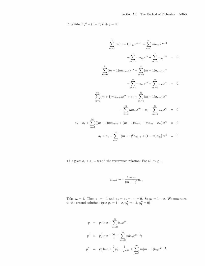
Section A.6 The Method of Frobenius A353
Plug into x y′′ + (1 − x) y′ + y = 0:
∞∑
m=1
m(m − 1)amxm−1 +
∞∑
m=1
mamxm−1
−∞∑
m=1
mamxm +
∞∑
m=0
amxm = 0
∞∑
m=0
(m+ 1)mam+1xm +
∞∑
m=0
(m+ 1)am+1xm
−∞∑
m=1
mamxm +
∞∑
m=0
amxm = 0
∞∑
m=1
(m+ 1)mam+1xm + a1 +
∞∑
m=1
(m+ 1)am+1xm
−∞∑
m=1
mamxm + a0 +
∞∑
m=1
amxm = 0
a0 + a1 +
∞∑
m=1
[(m+ 1)mam+1 + (m+ 1)am+1 −mam + am] xm = 0
a0 + a1 +
∞∑
m=1
[(m+ 1)2am+1 + (1 −m)am
]xm = 0
This gives a0 + a1 = 0 and the recurrence relation: For all m ≥ 1,
am+1 = − 1 −m
(m+ 1)2am.
Take a0 = 1. Then a1 = −1 and a2 = a3 = · · · = 0. So y1 = 1 − x. We now turnto the second solution: (use y1 = 1 − x, y′1 = −1, y′′1 = 0)
y = y1 lnx+
∞∑
m=0
bmxm;
y′ = y′1 lnx+y1x
+
∞∑
m=0
mbmxm−1;
y′′ = y′′1 lnx+2
xy′1 − 1
x2y1 +
∞∑
m=0
m(m− 1)bmxm−2.
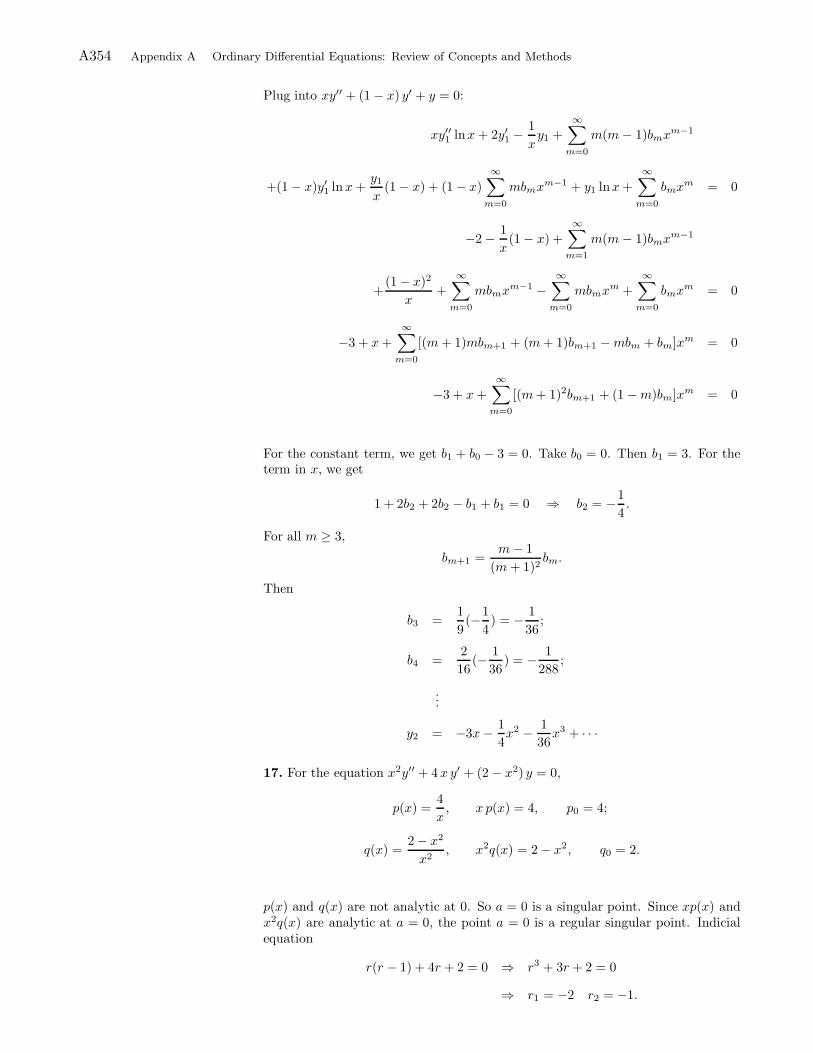
A354 Appendix A Ordinary Differential Equations: Review of Concepts and Methods
Plug into xy′′ + (1 − x) y′ + y = 0:
xy′′1 lnx+ 2y′1 −1
xy1 +
∞∑
m=0
m(m− 1)bmxm−1
+(1 − x)y′1 lnx+y1x
(1 − x) + (1 − x)
∞∑
m=0
mbmxm−1 + y1 lnx+
∞∑
m=0
bmxm = 0
−2 − 1
x(1 − x) +
∞∑
m=1
m(m− 1)bmxm−1
+(1 − x)2
x+
∞∑
m=0
mbmxm−1 −
∞∑
m=0
mbmxm +
∞∑
m=0
bmxm = 0
−3 + x+
∞∑
m=0
[(m+ 1)mbm+1 + (m+ 1)bm+1 −mbm + bm]xm = 0
−3 + x+
∞∑
m=0
[(m+ 1)2bm+1 + (1 −m)bm]xm = 0
For the constant term, we get b1 + b0 − 3 = 0. Take b0 = 0. Then b1 = 3. For theterm in x, we get
1 + 2b2 + 2b2 − b1 + b1 = 0 ⇒ b2 = −1
4.
For all m ≥ 3,
bm+1 =m− 1
(m+ 1)2bm.
Then
b3 =1
9(−1
4) = − 1
36;
b4 =2
16(− 1
36) = − 1
288;
...
y2 = −3x− 1
4x2 − 1
36x3 + · · ·
17. For the equation x2y′′ + 4 x y′ + (2 − x2) y = 0,
p(x) =4
x, x p(x) = 4, p0 = 4;
q(x) =2 − x2
x2, x2q(x) = 2 − x2, q0 = 2.
p(x) and q(x) are not analytic at 0. So a = 0 is a singular point. Since xp(x) andx2q(x) are analytic at a = 0, the point a = 0 is a regular singular point. Indicialequation
r(r − 1) + 4r + 2 = 0 ⇒ r3 + 3r + 2 = 0
⇒ r1 = −2 r2 = −1.
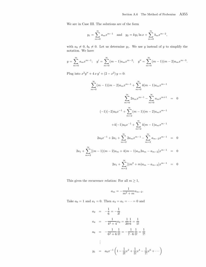
Section A.6 The Method of Frobenius A355
We are in Case III. The solutions are of the form
y1 =
∞∑
m=0
amxm−1 and y2 = ky1 lnx+
∞∑
m=0
bmxm−2,
with a0 6= 0, b0 6= 0. Let us determine y1. We use y instead of y to simplify thenotation. We have
y =
∞∑
m=0
amxm−1; y′ =
∞∑
m=0
(m− 1)amxm−2; y′′ =
∞∑
m=0
(m− 1)(m− 2)amxm−3.
Plug into x2y′′ + 4 x y′ + (2 − x2) y = 0:
∞∑
m=0
(m− 1)(m− 2)amxm−1 +
∞∑
m=0
4(m− 1)amxm−1
∞∑
m=0
2amxm−1 −
∞∑
m=0
amxm+1 = 0
(−1)(−2)a0x−1 +
∞∑
m=2
(m− 1)(m− 2)amxm−1
+4(−1)a0x−1 +
∞∑
m=2
4(m− 1)amxm−1
2a0x−1 + 2a1 +
∞∑
m=2
2amxm−1 −
∞∑
m=2
am−2xm−1 = 0
2a1 +
∞∑
m=2
[(m− 1)(m− 2)am + 4(m− 1)am2am − am−2]xm−1 = 0
2a1 +
∞∑
m=2
[(m2 +m)am − am−2]xm−1 = 0
This gives the recurrence relation: For all m ≥ 1,
am = − 1
m2 +mam−2.
Take a0 = 1 and a1 = 0. Then a3 = a5 = · · · = 0 and
a2 = −1
6= − 1
3!
a4 = − 1
42 + 4a2 =
1
20
1
6=
1
5!
a6 = − 1
62 + 6
1
5!= − 1
7 · 61
5!=
1
7!
...
y1 = a0x−1
(1 − 1
3!x2 +
1
5!x4 − 1
7!x6 + · · ·
)
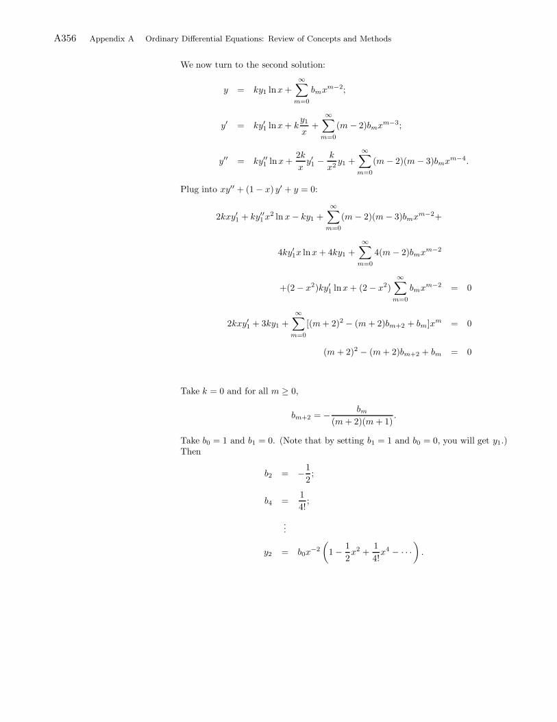
A356 Appendix A Ordinary Differential Equations: Review of Concepts and Methods
We now turn to the second solution:
y = ky1 lnx+∞∑
m=0
bmxm−2;
y′ = ky′1 lnx+ ky1x
+
∞∑
m=0
(m− 2)bmxm−3;
y′′ = ky′′1 lnx+2k
xy′1 − k
x2y1 +
∞∑
m=0
(m− 2)(m− 3)bmxm−4.
Plug into xy′′ + (1 − x) y′ + y = 0:
2kxy′1 + ky′′1x2 lnx− ky1 +
∞∑
m=0
(m− 2)(m− 3)bmxm−2+
4ky′1x lnx+ 4ky1 +
∞∑
m=0
4(m− 2)bmxm−2
+(2 − x2)ky′1 lnx+ (2 − x2)
∞∑
m=0
bmxm−2 = 0
2kxy′1 + 3ky1 +
∞∑
m=0
[(m+ 2)2 − (m+ 2)bm+2 + bm]xm = 0
(m+ 2)2 − (m+ 2)bm+2 + bm = 0
Take k = 0 and for all m ≥ 0,
bm+2 = − bm(m+ 2)(m+ 1)
.
Take b0 = 1 and b1 = 0. (Note that by setting b1 = 1 and b0 = 0, you will get y1.)Then
b2 = −1
2;
b4 =1
4!;
...
y2 = b0x−2
(1 − 1
2x2 +
1
4!x4 − · · ·
).