studies in chemical process design and synthesis. a ...€¦ · masoneilan handbook for control...

2304 Ind. Eng. Chem. Res. 1988, 27, 2304-2322

1 = in the stream/vapor condensation region 2 = in the condensate subcooling region

Literature Cited Buckley, P. S.; Luyben, W. L.; Shunta, J. P. Design of Distillation

Column Control Systems; Instrument Society of America: New York, 1985.

Cheung, T. F.; Luyben, W. L. "PD Control Improves Reactor Stability-. Hydrocarbon Process. 1979, Sept., 215-218.

Connell, J. R. "Realistic Control-Valve Pressure Drops". Chem. Eng. 1987, Sept, 123-127.

Luyben, W. L. Process Modeling, Simulation and Control for Chemical Engineers; McGraw-Hill: New York, 1973.

Masoneilan Handbook for Control Valves Sizing; Masoneilan In- ternational: New York, 1977.

Papastathopoulou, H. S. "Design and Control of Condensate- Throttling Reboilers". Master's Thesis, Department of Chemical Engineering, Lehigh University, 1987.

Shinskey, F. G. "When to Use Valve Positioners". Instrum. Control Syst. 1971, Sept, 11.

Shinskey, F. G. Distillation Control for Productivity and Energy Conservation, 2nd ed.; McGraw-Hill: New York, 1984.

Shinskey, F. G. Process Control Systems: Applications, Design, Adjustment; McGraw-Hill: New York, 1979.

Yu, C. C.; Luyben, W. L. "Analysis of Valve-Position Control for Dual-Input Processes". Ind. Eng. Chem. Fundam. 1986, 25,

Received for review March 15, 1988 Revised manuscript received July 13, 1988

Accepted July 31, 1988

344-350

Studies in Chemical Process Design and Synthesis. 8. A Simple Heuristic Method for the Synthesis of Initial Sequences for Sloppy Multicomponent Separations?

Shueh-Hen Chengj and Y. A. Liu* Department of Chemical Engineering, Virginia Polytechnic Insti tute and S ta t e University, Blacksburg, Virginia 24061

A simple heuristic method for the synthesis of initial sequences for sloppy multicomponent separations is proposed. In this type of separation, some components being separated may simultaneously appear in two or more product streams. Included in the proposed method are (i) effective and flexible tools for representing the synthesis problem, called the component assignment diagram (CAD), and for analyzing the technical feasibility of separation tasks or product splits, called the separation specification table (SST); (ii) practical design guidelines for the shortcut feasibility analysis of product splits; and (iii) simple rank-ordered heuristics for the synthesis of initial separation sequences. Of particular significance in the method is the quantitative consideration of the feasibility of product splits. The proposed method has been applied to a number of industrial separation problems. The results show tha t the heuristic method offers a simple and effective means for design engineers to generate several good initial sequences for sloppy multicomponent separations prior to the final heat integration and separator optimization.

1. Introduction An important process-design problem in multicompo-

nent separations is separation sequencing, which is concerned with the selection of the best method and sequence for the separation system. This problem has been covered in textbooks by King (1980, pp 710-720) and Henley and Seader (1981, pp 527-555). Reviews of recent studies on the subject can be found in Westerberg (1985) and Liu (1987).

Most of the published work on multicomponent separation sequencing has been limited to high-recovery or sharp separations, in which each component being separated appears in one and only one product stream. In industrial practice, however, it is often useful to permit some components to simultaneously appear in two or more product streams. This type of separation is called nonsharp or sloppy separation. Figure 1 compares two alternative schemes (sharp and sloppy) for the separation of a three-component mixture. We see that one more separator is needed in the sharp scheme than in the sloppy sequence.

* To whom correspondence should be addressed. ' Pa r t I of this series appears in AIChE J. 1985, 31, 487. Present address: Glitsch, Inc., P. 0. Box 660053, Dallas, TX

72566.

0888-5885/88/2627-2304$01.50/0

A typical chemical process usually comprises a reaction system and a separation system. The separation system generally involves reactant recovery, product separation, and waste and byproduct separations. As was pointed out by Douglas et al. (19851, the problem of flow-sheet synthesis can be posed as an optimization problem in which the reaction conversion is a key parameter for the optimum flow sheet. Further, there is an economic trade-off between high reactor costs and significant selectivity losses associated with high reaction conversions, which are balanced against large separation costs a t low reaction conversions. This implies that it may not be necessary to purify un- converted reactants to a high level prior to recycling them back to the reactor system. In other words, sloppy separations may be sufficient for many processes. The objective of this work is to present a simple heuristic method for the systematic development of initial sequences for sloppy multicomponent separations.

Section 2 introduces an effective and flexible framework for representing the problem of multicomponent separation sequencing. In particular, we propose a new representation, called component assignment diagram (CAD), to facilitate the identification of alternative separation tasks or product splits. In section 3, we analyze the technical feasibility of product splits based on component recovery specifications. Key developments in this section

1988 American Chemical Society

Ind. Eng. Chem. Res., Vol. 27, No. 12, 1988 2305

comp. now= 25 25 2s 25 i m ~ ~ ~ ~ / h ~ )

u E = l 2

D Blender

Figure 1. Comparison of sloppy and sharp separations.

are the introduction of a useful tool for feasibility analysis, called separation specification table (SST), and the pres- entation of some practical design guidelines to facilitate the shortcut feasibility analysis of product splits by using the well-known Fenske equation (Fenske, 1932). Section 4 describes our rank-ordered heuristics for the synthesis of initial separation sequences, and section 5 presents the results of applying the proposed heuristic method to a number of industrial separation problems. Finally, section 6 compares the proposed method with other approaches reported in the literature and summarizes the conclusions from this work. For convenience, sepcifications for feed and product streams of all illustrative examples are summarized in Appendix A.

2. Problem Representation 2.1. Component Assignment Diagram (CAD). Fig-

ure 2 illustrates a CAD for representing example 1. In constructing the CAD for a given synthesis problem, all components are first placed from left to right, in order of decreasing separation factor or relative volatility. Hori- zontal product lines (PLs) are then used to separate one product stream from the other. Each PL corresponds to a separation task or product split. For convenience, we write down all candicates for current splits on the righ- hand side of a CAD, and flow rates of all product streams on the left-hand side.

Vertical component lines (CLs) specify the component split or distribution in each product stream. The length of the CL represents the flow rate of a component in the specific product stream bounded by two PLs. The nu- merical value of the component flow rate is indicated next to each CL. Also, a full CL connecting two adjacent PLs implies that the component represented by that line is the most plentiful component in that product stream; there must be at least one full CL between two adjacent PLs.

2.2. Arrangement of Product Sets. For any two product streams in a CAD, the product with the more volatile component(s) or more plentiful of the most volatile component is placed at a position lower than others. This simply means that if component i is the most volatile

product streams SPllIS - comp = A B C D imolerlhr)

15 0 I l6 I 4

Figure 2. CAD for representing example 1: CL = component line; PL = product line.

species in two adjacent product streams, then those products are to be arranged in a CAD such that

Here ni,k is the flow rate of the ith component in the kth product stream and k is the product stream number re- flecting the position of a product stream on a CAD, counting from bottom to top. If two product streams have an equal amount of the most volatile component (in both products), we should pay attention to the next volatile component to decide which product is more volatile.

As an illustration, let us consider the CAD of Figure 2, starting with the most volatile component, A, which appears in product streams 1 and 2. Since nA,l = 15 mol/h, nA:, = 10 mol/h, and nAJ1 > nA,2, we place product stream 1 in the CAD at a position lower than that of product stream 2. Having specified the positions of product streams 1 and 2, we next focus our attention on product streams 2 and 3. Figure 2 shows that the most volatile component in product stream 2 is component A, and the most volatile component in product stream 3 is component C (which is less volatile than component A). Thus, product stream 2 is more volatile than product stream 3. We then put product stream 3 above product stream 2 to indicate the relative magnitude of product volatility. In a similar manner, the remaining product stream, 4, can be posi- tioned.

2.3. Sloppy and Sharp Separations. On the right- hand side of Figure 2, we see three candidates for the initial separation for obtaining product streams 1-4 in example 1, namely, 12314,12134, and 11234. These sloppy separations are represented on the CADS shown in Figure 3a-c. We classify sloppy separations into two categories by introducing the concept of split point (SP). As illustrated in Figure 3a, a split point represents an intersection point between a horizontal product line (PL) and a vertical component line (CL) that crosses over two adjacent product streams. The existence of an SP on the CL for component D in Figure 3a indicates that component D is distributed in two product streams, (123) and 4. In this work, we call those sloppy separations with one split point or one distributed component the single-split-point (SSP) or single-distributed-component (SDC) sloppy separations. Thus, both parts a and b of Figure 3 correspond to SSP sloppy separations.

Figure 3c shows a sloppy separation with more than one split point or distributed component, and it represents the second class, called the multiple-split-point (MSP) or multiple-distributed-component (MDC) sloppy separations. In this figure, we see three split points, SPl-SP3, indicating that three components (A, B, and C) are distributed in two product streams, 1 and (234).

Ind. Eng. Chem. Res., Vol. 27, No. 12, 1988

component flow - 25 25 25 25 product split

streams - A B C D -

(molerihr)

I 15 4 D

15 1 PL

6- - - 1 2 3 4 Split Point (SP)

(123):ABCD CL

as

A B C D I

(34):CD

e--- 12/34

55 (1 2):ABC

t A B C D

8 7 5 1 I *n I I

(ABCD)

ABCDID + - - - 5 7 5 1 5 15 I 25 I 12.5 [ PL

D

Figure 3. Examples of CADS for sloppy and sharp separations. (a and b) Single-split-point (SSP) or single-distributed-component (SDC) sloppy separations. (c) Multiple-split-point (MSP) or multiple-distributed-component (MDC) sloppy separation. (d) An alternative representation of case (c), noting the disappearance of split point SPs due to vertical downward shift of component line for C within product stream 1. (e) Sharp separation of ABCD into ABC and D as represented by using a vertical product line or split line. (f) An SSP sloppy separation with the split point (SP) or distributed component A corresponding to the most volatile component.

I t is important that we pause to give a word of caution regarding the "apparent" number of split points and the number of distributed components. Figure 3d depicts an alternative representation of Figure 3c. On comparing both figures, we see that split point SP3 in Figure 3c can no longer be identified easily in Figure 3d. This is a result

of the vertical downward shift of a segment of the CL for component C within product stream 1. Note that each segment of CL for a component can be freely moved up- ward or downward within a product stream. Since we see in Figure 3d two segments of the CL for component C, with each segment appearing in one product stream, it is obvious that component C is a distributed component. Therefore, although Figure 3d has apparently one less split point than Figure 3c, both figures actually represent the same sloppy separation.

The preceding comparison illustrates an important point regarding the CAD for sloppy separations. That is, the key characteristic for identifying a sloppy separation is the appearance of multiple segments of a CL for a component. This appearance indicates that the component represented by the CL is a distributed component in several product streams.

Figure 3e shows a CAD for representing a sharp separation of a mixture ABCD into ABC and D. For sharp separations, each CL for a component appears in one product stream only. Also shown in the figure is a dashed vertical product line that gives an identical product set (ABC and D), as does the horizontal product line labeled by PL. Vertical product lines on a CAD are used to separate components, and they always represent sharp separations; horizontal product lines are employed to separate product streams, and they represent either sloppy or sharp separations depending on the component recovery specifications. Part 9 of this series (Cheng and Liu, 1988) describes the combined use of vertical and horizontal product lines for the synthesis of multicomponent separation sequences incorporating both sharp and sloppy separators.

In this work, we classify sloppy separations into three groups: (1) pseudosharp (PS); (2) semisharp (SS) ; and (3) nonsharp (NS). This classification is based on the values of key component recovery fractions in the overhead (denoted by dLK and dHK for the light key and heavy key, respectively) and in the bottoms (denoted by bm and ~ H K ) . For example, we specify 0.95 < dLK < 0.98 for PS, 0.80 < dLK < 0.95 for SS, and dLK < 0.80 for NS. Using the ratio of key-component recovery fraction in the overhead to that in the bottoms, that is, (d/b)LK for the light key and (d/b)HK for the heavy key, we can also specify the above classification in the following fashion. (1) pseudosharp (PS):

(d/b)LK N 19 (=0.95/0.05) to 49 (=0.98/0.02) (2) and (d/b)HK N 0.0204 (=0.02/0.98) to 0.0526 (=0.05/0.95)


Table I. Separation Specification Table (SST) for Final Splits i n Example 1 Represented by the Component Assignment Diagram (CAD) of Figure 5"

separation ovhd/ btm LK/HK A, "C ( ~ / ~ ) L L K I ( d / b ) ~ ~ @ / ~ ) H K ( ~ / ~ ) H H K I

36.6 0.6/0.4 I 0.5/0.5 0.98/0.02 32.7 0.6jO.S 0.5/0.5 I 0.98/0.02

NS(MSP) 112 A/B 1/2 B/C

S SS(SSP)

2/3 314

" NS : nonsharp separation, MSP = multiple split point, S = sharp separation, SS = semisharp separation, SSP = single split point, ovhd = overhead, btm = bottoms. Dashed vertical lines designate boundaries between light-key (LK) and heavy-key (HK) components. Dashed horizontal lines represent approximate values. Solid horizontal lines denote infeasible specifications.

1234

1/23

1 2/3

2314 2/34 1/2 314

112

Figure 4. Decision tree of candidates for product splib in example 1.

3. Feasibility Analysis 3.1. Separation Specification Table (SST). Figure

4 shows a decision tree for example 1, listing candidates for product splits that we may consider in separating feed ABCD into product streams 1-4. This figure includes the following product splits: (a) first splits, 11234, 12/34, 12314; (b) second splits, 1123,1213, 2/34, and 2314; and (c) third or final splits, 112, 213, and 314. Since not all splits may be technically and/or economically feasible, we present below some simple methods to systematically examine the feasibility of product splits.

Let us consider, for example, the feasibility of candidates for final splits (112, 213, and 314). Figure 5 illustrates the CADs for these candidates. To facilitate the examination of feasibility of product splits, we propose a separation specification table (SST) for use in conjunction with the CAD. Table I gives an example of an SST corresponding to CADs for candidates for final splits in example 1 shown in Figure 5.

An SST contains the following information: (1) types of separations; (2) overhead and bottoms product streams; (3) choice of light-key (LK) and heavy-key (HK) compo- nenets; (4) separation factor between the LK and HK; and (5) calculated and estimated ratios of component split in the overhead to that in the bottoms.

In an SST, a dashed vertical line is used to designate the boundary between the LK and HK. We shall present some guidelines on choosing LK and HK components in sections 3.3 and 3.4A. Let us illustrate how to calculate or approximate component split ratios, ( d / b ) s , listed in Table I based on component flow rates shown in Figure 5.

Consider, for example, final product split 112 with A/B as LK/HK. We find ( d / b ) L K = ( d / b ) A = 15/10

0.6/0.4 (Table I) ( d / b ) H K = ( d / b ) B = 12.5/12.5

0.5/0.5 (Table I) ( ~ / ~ ) H H K I = ( d / b ) c =

5/0 (Figure 5a) E 0.98/0.02 (Table I) Here, subscript HHKl refers to the first heavier-than-

(Figure 5a) =

(Figure 5a) =

Product B C streams A

t -

2:AB

15 1:ABC

I I w

A B C D

C D

15 4:D

I sp 3:CD

L I

Figure 5. CADs for candidates for final splits in example 1. (a, top) Split 1 /2 with A/B and B/C as candidates for LK/HK. (b, middle) Split 2/3 with C/D as LK/HK. (c, bottom) Split 3/4 with C/D as LK/HK.

heavy key or heavy component. In the above calculations, component flow rates in the overhead and bottoms shown in Figure 5a are converted to equivalent component recovery fractions in the overhead and bottoms such that di + bi = 1. The resulting values of d j and bi are used to find component split ratios, ( d / b ) s , as listed in the SST of Table I. For the last component split ratio listed above, we use a limiting split ratio of 0.9810.02 to approximate the "sharp" cut represented by the calculated component split, 510. Similarly, for the same product split 112 with B/C as LK/HK, we designate components A, B, and C as LLK1, LK, and HK, respectively, and specify the same ( d / b ) s as above, namely, 0.6/0.4,0.5/0.5, and 0.98/0.02 in Table I.

For final product split 213 with B/C as LK/HK listed in Table I, we find ( d / b ) ~ ~ = ( d / b ) c =

12.5/0 (Figure 5b) N 0.98/0.02 (Table I)

( d / b ) ~ ~ = ( d / b ) ~ = 0/25 (Figure 5b) E 0.02/0.98 (Table I)

Here, we use a limiting ratio of 0.9810.02 to approximate the sharp cut represented by the calculated component split ratio, 12.510, for the LK or component C. Likewise,

2308 Ind Eng. Chem. Res., Vol. 27, No. 12, 1988

we use 0.02/0.98 to approximate the calculated component split ratio, 0/25, for the HK or component D.

For final product split 3/4 with C/D as LK/HK, we can readily identify the following correspondence between Figure 5c and Table I: ( d / b ) I K = i d / h ) c =

20/0 (Figure 5c) N 0.98/0.02 (Table I)

10/15 (Figure 5c) 0.4/0.6 (Table I) 3.2. Infeasible Splits Due to Component Recovery

Specifications. The use of SST provides a convenient way to examine the feasibility of product splits based on component recovery fractions, d, and b,. Consider, for example, a mixture with the following components arranged in order of decreasing separation factors or relative volatilities: ..., LLK3, LLK2, LLK1, LK, HK, HHK1, HHK2, HHK3; splits associated with these components are said to be feasible provided that ... ~ L L K , ~ L L K I > ~ L K ~ H K >

or ... < ~ L L K Z < ~ L L K I < ~ L K < ~ H K <

bHHKl < bHHKZ < ... (8) These two inequalities can be verified by considering the well-known Fenske equation (Fenske, 1932):

( d / b ) H K = ( d / b ) D =

d H H K 1 > ~ H H K Z > ... (7)

(9)

In this equation, N,,, is the minimum number of theoretical stages and aLK,HK is the relative volatility between the LK and HK. Since N,,, and log CYLKHK are both positive, eq 9 gives

log [ ( d / b ) L K ( b / d ) H K ] ~ ~ I n I r l =

log ~ L K , H K

log [ ( ~ / ~ ) L K ( ~ / ~ ) H K I > 0 Or ( d / b ) L K ( b / d ) H K > 1

On the basis of the relationships among component recovery fractions, we replace d H K by (1 - d L K ) and bHK by (1 - dHK) and write

~ L K 1 - ~ H K > 1 ___- 1 - d ~ ~ ~ H K

or d L K ( 1 - d H K ) > (1 - d L K ) d H K

This results in a simple inequality: d,K > dHK. To verify other inequalities in eq 7 and 8, we note that the Fenske equation is also applicable to different combinations of light and heavy components such as (LLKB,HK), (LLKl,HK), (LK,HHKl), and (LK,HHKB). This follows because of the straight-line relationship on a log-log plot of component split ratio, d/b, versus relative volatility, cy,

(see straight line 1 in Figure 8). Thus, by repeatedly applying the Fenske equation to different light-heavy component pairs, we can readily verify all inequalities in eq 7 and 8.

As an illustration, let us apply eq 7 and 8 to the SST for final splits in example 1. Table I indicates that for product split 1 / 2 with A/B as LK/HK,

dlK > d H K p‘ d H H K l (0.6 > 0.5 0.98) (10)

b 1 ~ < b,, 4 b H H K l

and with B/C as LK/HK, d , ,~ , > d,, # d H K

bLLKl < bLK 4 b H K

(0 4 < 0.5 $ 0 02)

(0 6 > 0 5 3 0.98)

(11)

(12)

(13)

Since neither eq 7 nor eq 8 is satisfied, product split 1 / 2

(0 4 < 0 5 4 0.02)

with A/B or B/C as LK/HK is infeasible due to component recovery specifications.

In what follows, we present some guidelines on the selection of LK and HK components and then consider another aspect of infeasible splits due to undesirable nonkey-component distributions.

3.3. Choice of Light-Key (LK) and Heavy-Key (HK) Components. Key components for sharp separations are commonly described by the following statement (Coulson et al., 1980): “The light key (LK) is the lightest component appearing in the bottoms and the heavy key (HK) is the heaviest component in the distillate (or overhead).” When dealing with sloppy separations, however, it is not always possible to use this definition to identify key components. For example, by applying the definition to the split shown in Figure 3b, we find that distributed component C is not only the lightest component in the bottoms but also the heaviest component in the overhead. We therefore end up with an indeterminate situation of C = LK and C = HK. In the following, we suggest three rules for specifying key components in sloppy separations. These rules are fairly general and have been found to be effective to aid in the selection of proper LK and HK components in a large number of sloppy separation problems (Cheng, 1987).

Rule 1. Most splits have a distinctive discontinuity of the component split ratio, d/b. Choose the LK and HK to fall adjacent to each other around this discontinuity.

Consider, for example, the following split ratios:

component A B l C D d/b 0.99/0.01 0.975/0.025 j 0.025/0.975 0.01/0.99

Here, we observe a discontinuity of d/b between components B and C, since dA > bA and dB > dg, while for components C and D, dc < bc and d D < bD. Thus, a dashed vertical discontinuity line can be drawn between components B and C. Two components immediately adjacent to that line, whose split ratios are within the range of pseudosharp splits defined by eq 2 to 3, are treated as key components (LK = B and HK = C, in this case).

Rule 2. For a single-split-point (SSP) sloppy separation where the split point or distributed component corresponds to the most volatile or least volatile component, choose the distributed component and its neighboring component as keys.

As an illustration, Figure 3f shows an SSP sloppy separation with the most volatile component, A, being distributed in both overhead and bottoms products for product split ABCD/D. Rule 2 suggests that keys are A(LK) and B(HK).

Rule 3. For other types of SSP sloppy separations and for multiple-split-point (MSP) sloppy separations, there exist several candidates for LK/HK. Component distributions resulting from different sets of LK/HK should be examined by the Fenske equation. The set of LK/HK that avoids undesirable distributions (or splits) of nonkey components in both overhead and bottoms products is recommended as the choice of LK/HK.

Figure 3b depicts an SSP sloppy separation where the split point (labeled SP) or the distributed component (component C) corresponds to neither the most volatile nor the least volatile component for product split 12/34. In this case, candidates of LK/HK for product split 12/34 are B/C, C/D, and B/D. These three choices of LK/HK are illustrated in Figure 6 and will be examined further in the following section.

Figure 3c illustrates an MSP sloppy separation where two of the split points (labeled SP2 and SP3) or distributed components (components B and C) represent neither the


is to properly specify the distributions of nonkey components in both overhead and bottoms products. As part of our work, we have carried out a comparative study of rigorous simulation and shortcut modeling of multicomponent distillation columns for sloppy separations. An objective of the study was to obtain an improved quantitative understanding and some practical design insights of the characteristics of nonkey component distributions in sloppy separations. Another objective was to identify simple design heuristics that provide an adequate knowledge of nonkey component distributions through a shortcut modeling by the Fenske equation.

Rigorous plate-to-plate simulations using a commercial computer-aided design package, DESIGN I1 (ChemShare Corporation, 1985), have been conducted to identify how nonkey component distributions behave. As an illustration, Figure 7a shows a log-log plot of selected key and nonkey component split ratios versus component relative volatility in example 2A over a wide range of operating reflux ratios (RD = 1.05-1.80R~,,b). In this example, we specify (d/b)LK = 0.710.3 and (d /b )HK = 0.02/0.98, which correspond to a semisharp sloppy separation. For the nonkey component or the lighter-than-light key, LLK1, we see from the figure that at RD = 1.05R~m, log ( d / b ) m l N 0.75 or d / b c1 5.5 = 0.846/0.154. This result indicates that about 84.6% LLKl appears in the overhead and 15.4% LLKl goes to the bottoms. Thus, LLKl is distributed in both overhead and bottoms in finite amounts, and this observation is valid over a wide range of operating reflux ratios as depicted in Figure 7a. This figure also demonstrates that, because of the possibility of undesirable nonkey component distributions in sloppy separations, it is not always correct to assume the operating reflux ratio as being approximately 1.1 times the minimum reflux ratio, RD,min [see, for example, Muraki and Hayakawa (198S)l. Rigorous computer simulations are often required to identify the proper operating reflux ratios in sloppy separations.

To eliminate the undesirable distribution of nonkey component LLKl in both overhead and bottoms products, we increase the number of theoretical stages ( N ) a t a constant reflux ratio (RD = 1.5RD,min = 0.815). Our hope is that essentially all (say, 99.5%) of LLKl goes to the

A B C D T I

A B C D I

Figure 6. An illustration of choices of LK/HK for the single- split-point (SSP) sloppy separation 12/34 shown in Figure 3b. LK = light key, HK = heavy key, LLK = lighter-than-light key, HHK. = heavier-than-heavy key, and IC = intermediate component between the LK and HK.

most volatile nor the least volatile component for product split 1/ 234.

3.4. Shortcut Feasibility Analysis of Nonkey Com- ponent Distributions. A. Choice of LK/HK and Undesirable Distributions of Nonkey Components. Rule 3 of the preceding section suggests that we choose LK/HK such that undesirable distributions of nonkey components in both overhead and bottoms products can be avoided. We discuss below the basis of this recom- mendation together with illustrative examples.

We note first that a difficult problem in the design of multicomponent distillation columns for sloppy separations

I , I / ,

1 I I

I I I 1

K R I 2 / * I i I /

1

* I 1 I 1

a +. a oo a, Lo a +, a o1

I ' i I I 1 ,J ; ! I 1 1 ~ " I i

u/ 0 - - a - * 70 =

Figure 7. (a, left) Illustration of selected key and nonkey component distributions in a semisharp sloppy separation in example 2A as a function of operating reflux ratio range 1.05-1.80R~,-: ( ~ l / b ) ~ K = 0.7/0.3 and (d/b)HK = 0.02/0.98. (b, middle) Effect of the number of theoretical stages, N , on selected key and nonkey component distributions in a semisharp sloppy separation in example 2A at a constant reflux ratio R D = 0.815 = 1.05R~,,, ( d / b ) m = 0.7/0.3, and (d/b)HK = 0.02/0.98. (c, right) Effect of the number of theoretical stages, N , on the split ratio, ( d / b ) , of nonkey component, LLK1, in both overhead and bottoms product in example 2A shown in Figure 7b. Note that the desired split ratio, ( d / b ) m ~ ~ = 0.995/0.005, or log ( d / b ) ~ ~ ~ l = 2.3 cannot be reached even with a very large number of theoretical stages ( N > 60).

LOB. LOG 0

2310 Ind. Eng. Chem. Res., Vol. 27, No. 12, 1988

LOG a,

Figure 8. Distributions of key and nonkey components versus relative volatility a t different operating reflux ratios (Stupin and Lockhart, 1968; King, 1980).

overhead and very little (say, 0.5%) of LLKl appears in the bottoms, resulting in a desired split ratio (d /b)LLK1 = 0.995/0.005, or log (d/b)LLK1 = 2.3. Figure 7b shows that, as N increases, nonkey component LLKl becomes less distributed; however, Figure 7c indicates that the desired split ratio, log (d/b)LLK1 = 2.3, cannot be reached even with a very large number of theoretical stages (N > 60).

This example shows that in order to avoid undesirable distributions of nonkey components in both overhead and bottoms products, it may be necessary to use a distillation column with a large number of theoretical stages, resulting in a costly design. In addition, the sensitivity of nonkey component distributions to the reflux ratio may give rise to operational problems. Therefore, certain choices of LK/HK that may lead to undesirable distributions of nonkey components are not favored.

B. Practical Bounds on Split Ratios of Nonkey Components. King (1980) has summarized the findings of Stupin and Lockhart (1968) on product split specifications in multicomponent distillation and plotted log ( d / b ) i versus log ai, as shown in Figure 8, for cases where split ratios of both keys are pseudosharp that satisfy eq 2 and 3. As RD is reduced from the total-reflux condition, RD,,, the component distribution first moves away from the minimum-reflux curve (curve 4). This component distribution thus appears outside the region bounded by the component distributions at total reflux RD,, (straight line 1) and at minimum reflux RD,min (curve 4). When R D is lowered to approximately 5RD,min, the component distribution approaches curve 2. As RD is further reduced, the component distribution moves backward toward the total-reflux "curve" (straight line 1) into the bounded region and approaches curve 3 when RD = l.lRD,-. At common operating reflux ratios ( l . lRD,min < R D < 1.5RD,min), component distributions are bounded by straight line 1 (at RDJ and curve 3 (at RD = l.lRD,mp).

The latter observation is practically significant for specifying the split ratios of nonkey components in sloppy separations. In particular, close inspection of Figure 8 shows that, for light components (LLKs) in region C, component split ratios represented by straight line 1 a t total reflux predicted by the Fenske equation give lower

bounds on split ratios for LLKs at common operating reflux ratios (l . lRD,min < RD < Likewise, for heavy components (HHKs) in region A, component split ratios represented by straight line 1 predicted by the Fenske equation give upper bounds on split ratios for HHKs at common operating reflux ratios. In other words, at common operating reflux ratios,

( ~ / ~ ) L L K > ( ~ / ~ ) L L K , L B (14)

( ~ / ~ ) H H K < ( ~ / ~ ) H H K , u B (15)

In these equations, ( d / b ) , and (d/b)= are, respectively, exact split ratios of light component LLK and heavy component HHK obtained from the rigorous simulation at common reflux ratios RD = 1 . 1 - 1 . 5 R ~ , ~ ~ ~ . ( ~ / ~ ) L L K , L B and ( ~ / ~ ) H H K , U B are, respectively, the lower bound (LB) for the split ratio of LLK and the upper bound (UB) for the split ratio of HHK obtained from the shortcut modeling by the Fenske equation at the total-reflux condition

Equations 14 and 15 suggest a simple way to identify the proper choice of LK/HK that avoids undesirable distributions of nonkey components in both overhead and bottoms products. Thus, we first modify both equations as follows: (a) condition for LLK to be nondistributed

and

R D = Rq,.

( ~ / ~ ) L L K > ( ~ / ~ ) L L K , L B > 0.98/0.02 (16) (b) condition for HHK to be nondistributed

( ~ / ~ ) H H K < ( ~ / ~ ) H H K , u B < 0.02/0.98 (17) The inequality (d/b)mKbB > 0.98/0.02 simply says that

split ratios predicted by the Fenske equation at total reflux are greater than the limiting ratio of 0.98 J0.02 for light components. The latter implies that most of light components appear in the overhead product and very little of them go to the bottoms product. In other words, light components (LLKs) are nondistributed in both overhead and bottoms products. Likewise, the inequality ( d l b)HHK,$B < 0.02/0.98 implies that heavy components (HHKs) are nondistributed in both products.

When evaluating a certain choice of LK/HK, we can use a shortcut analysis by the Fenske equation at total reflux to check if a resulting light component (LLK) is nondistributed in both overhead and bottoms products, that is, if ( ~ / ~ ) L L K , L B > 0.98/0.02 is satisfied. If this inequality is valid, then split ratios of light components (LLKs) at common operating reflux ratios are also greater than 0.98/0.02 according to eq 16. This choice of LK/HK avoids undesirable distributions of light components (LLKs) in both overhead and bottoms products. In a similar fashion, we can use eq 17 to eliminate certain choices of LK/HK when the likelihood of having distributed heavy components (HHKs) is observed after applying the Fenske equation a t total reflux.

C. An Illustrative Example of Shortcut Feasibility Analysis of Nonkey Component Distributions. Let us now apply the Fenske equation to analyze the feasibility of product splits corresponding to three candidates for LK/HK shown in Figure 6 for the SSP sloppy separation represented by the CAD of Figure 3b. From the latter figure, we see that desired component split ratios are ( d / b ) A = (d/b)B =

25/0 (Figure 3b) > 0.98/0.02 (Table 11) ( d / b ) , = 5/20 (Figure 3b) = 0.2/0.8 (Table 11)

( d / b ) , , = 0/25 (Figure 3b) > 0.02/0.98 (Table 11)


Table 11. Illustration of Shortcut Feasibility Analysis of Product Splits Corresponding to Three Candidates for LK/HK Shown in Figure 6 for the Single-Split-Point Sloppy Separation of Figure 3b

svlit ovhd/btm LK/HK ( d / b ) n ( d / b ) n ( d / b ) c ( d / b ) n feasibility desiredo 12/34 >0.98/0.02 >0.98/0.02 0.2/0.8 <0.02/0.98 shortcut anal.: case 1 12/34 B/Cb >0.999/0.001 -O_.%JO_._qZ_. 0.2/0.8 0.002/0.998 feasible

12/34 C/Dc 0.983/0.017 0.786/0.214 0.2/0.8 - 0.02_/0.98 - - - - - - - infeasible 12/34 BIDb >0.999/0.001 !3,9_ll3,4- 0.301/0.699’ - 0.0210.98 - - - - - - infeasible

0.0110.99 infeasible 12/34 B/D >0.999/0.001 _ 0 1 9 _ 9 ~ ~ . _ 0 ~ - 0.297/0.703 - 0.01/0.99 - - - - - - infeasible

12/34 C/D 0.999/0.001 0.943/0.057 0.2/0.8 - 0.005j0.995 - - - - - - - infeasible 12/34 B/D >0.999/0.001 _019_9_5/O_._Oo5_ 0.295/0.705 -O,[email protected]!35 infeasible

shortcut anal.: case 4 12/34 B/C >0.999/0.001 _O~spl_o,O_~~ 0.2/0.8 0.0001/0.9999 feasible 12/34 C/D >0.999/0.001 0.989/0.011 0.2/0.8 - O.OO_li_o,sP_g -- feasible 12/34 B/D >0.999/0.001 $sp_si_Olo_41- 0.293/0.707 !.12@l]-OL2~2 infeasible

shortcut anal.: case 2 12/34 B/C >0.999/0.001 0.99/0.01 0.2/0.8 0.001/0.999 feasible 12/34 C/D 0.996/0.004 0.887/0.113 0.2/0.8 - - - - - - -

shortcut anal.: case 3 12/34 B/C >0.999/0.001 _olsp_5 f 0_.005_ 0.2/0.8 0.0005/0.9995 feasible

“From Figure 3b, ( d / b ) , = ( d / b ) , = 25/0 > 0.98/0.02, ( d / b ) c = 5/20 = 0.2/0.8, and ( d / b ) , = 0/25 < 0.02/0.98. “See Figure 6a-c, respectively. ‘ d / b for sharp LK is set at 0.98/0.02, 0.99/0.01, 0.995/0.005, and 0.999/0.001 for case 1 to case 4, respectively; d / b for sharp HK is fixed at 0.02/0.98, 0.01/0.99, 0.005/0.995, and 0.001/0.999 for case 1 to case 4, respectively. These specifications are underlined by dashed horizontal lines. ’Solid horizontal lines denote infeasible product splits (that is, undesirable nonkey-component distributions).

Consider, for example, the results of shortcut feasibility analysis for case 1 listed in Table 11. Three candidates for LK/HK are included.

(a) When LK = B and HK = C (Figure 6a), the split ratio of the sharp LK, (dlb),, is assumed to be 0.98/0.02 and the split ratio of the semisharp HK, (d /b )c , is given as 0.2/0.8. The Fenske equation gives (d/b)LLK = (d /b)A

shortcut results satisfy the desired component split ratios. Therefore, split 12/34 with B/C as LK/HK is feasible.

(b) When LK = C and HK = D (Figure 6b), ( d / b ) c is given as 0.2/0.8 and ( d / b ) D is assumed to be 0.0210.98. Applying the Fenske equation gives (d/b)LLK1 = ( d / b ) A = 0.983/0.017 and (d /b)LLKP = ( d / b ) , = 0.786/0.214. Un- fortunately, the latter estimate of the split ratio for component B does not satisfy the desired specification (>0.98/0.02). Consequently, split 12/34 with C/D as LK/HK is infeasible.

(c) When LK = B and HK = D (Figure 6c), component C appears as an intermediate component (IC) being distributed in both overhead and bottoms products. Here,

= (d /b ) , = 0.02/0.98. The Fenske equation gives ( d / b ) , = ( d / b ) A > 0.999/0.001 and ( d / b ) I c = ( d / b ) c = 0.301/ 0.699. The latter represents an undesirable distribution of nonkey component C in both overhead and bottoms products, and it is not recommended. Therefore, split 12/34 with B/D as LK/HK is considered to be infeasible.

Cases 2-4 listed in Table I1 present results of shortcut feasibility analysis when the split ratio of the sharp LK, ( d / blLK, is gradually increased to 0.99/0.01, 0.995/0.005, and 0.999/0.001 and when the split ratio for the sharp HK, (d /b )HK, is slightly decreased to 0.01/0.99,0.005/0.995, and 0.001/0.999. The results are similar, except that for case 4, split 12/34 with C/D as LK/HK becomes feasible with (d /b )c = 0.2/0.8 and (d/b)D = 0.001/0.999. However, the latter split ratio for component D represents a very stringent key-component recovery requirement, and it is not recommended for use in the design of distillation columns for sloppy separations.

On the basis of the results from this example and from our comparative study of rigorous simulation and shortcut modeling of sloppy separations (Cheng, 1987), we offer the following guideline: “For the purpose of examining the feasibility of nonkey component distributions by applying the Fenske equation, the recommended split ratio for a sharp LK or HK for sloppy splits, regardless of their sloppiness, to be used to find nonkey component distributions is ( d / b ) L K = 0.98/0.02 or ( d / b ) H K = 0.02/0.98.”

> 0.999/0.001 and ( d / b ) H m = ( d / b ) ~ = 0.002/0.998. Both

we assume that (d/b)LK = (d/b)B 0.98/0.02 and (d/b)HK

An important implication of this guideline is that only case 1 needs to be considered in Table 11. This obviously greatly simplify the work involved in the shortcut feasibility analysis of nonkey component distributions.

3.5. Transformation of an Infeasible Product Set into Equivalent Feasible Product Sets. Consider again the CADS of Figure 5 that represent three candidates for final splits in example 1. As shown earlier, product split 1/2 with either A/B or B/C as LK/HK is technically infeasible. Product streams 1 and 2 are designated an infeasible product set, denoted by (1,Z). In what follows, we demonstrate how to transform an infeasible product set into equivalent product sets representing feasible separation tasks. These tasks can eventually give the specified product streams through stream splitting and blending.

The left portion of Figure 9a shows a CAD for example 1, and the lower portion depicts the final split of 1/2. In the figure, we enclose in a dashed envelope specified flow rates of components B and C, for which corresponding component recovery specifications lead to the infeasible product set, (1,2). As illustrated in the right portion of Figure 9a, this infeasible product set can be transformed into an equivalent feasible product set (1*,2,1’) by splitting part of product stream 1 into two pseudoproduct streams, 1* and 1’. Since all component recovery fractions corresponding to component flow rates in the equivalent product set (1*,2,1’,3,4) satisfy eq (7) and (8), product splits (1*/2,2/1’,1’/3,3/4) depicted in the right portion of Figure 9a are technically feasible based on component recovery specifications. After carrying out these splits, desired product stream 1 can be readily obtained by blending together pseudoproduct streams 1* and 1’.

This example illustrates the transformation of an infeasible product set into an equivalent feasible product set by incorporating SSP sloppy splits illustrated previously in Figure 3a,b. Two other approaches incorporating MSP sloppy splits and sharp splits are shown in parts b and c of Figure 9, respectively. Since the transformation available is generally not unique, we suggest the following two rules for choosing an approach to convert an infeasible product set into equivalent feasible product sets.

Transformation Rule 1. Favor the case with the fewest number of pseudoproducts to minimize the number of required product splits or separation tasks.

Transformation Rule 2. Favor the feasible product set corresponding to a nonsharp separation over that leading to a semisharp separation. Likewise, favor the product set resulting with a semisharp separation over that

Ind. Eng. Chem. Res., Vol. 27, No. 12, 1988

S t r e a m

1 5 4 D

20 l o 3 C D I - .

I \

: 5 : 1 'C

t- sharp . r

10 1 2 5 2 AB

15 l Z 5 l * : A B

P,Cd"Cl

I-

! 2~ I

20 I

15 I ABC

.- ?.AB

l * : A

I 1 5 1 4 D I

Figure 9. Transformation of an infeasible product set into equivalent feasible product sets: separating intermediate product stream (12) obtained from split 12/34 in example 1 represented by the CAD of Figure 2 into individual product streams 1 and 2: (a) by incorporating single-split-point (SSP) sloppy splits; (b) by incorporating multiple-split-point (MSP) sloppy splits; (c) by incorporating sharp splits.

giving a sharp separation. In other words, the separations resulting from introducing pseudoproduct streams are preferred in the following decreasing ranked order:

NS (nonsharp) > SS (semisharp) > S (sharp) (18)

Applying transformation rule 2 and eq 18 to example 1 suggests that the transformation incorporating sloppy splits illustrated in Figure Sa is preferred over that incorporating sharp splits depicted in Figure 9c.

3.6. Use of Stream Bypassing To Reduce the Mass Load of Downstream Separation. Let us illustrate the use of stream bypassing to reduce the mass load of downstream separation by considering example 1 represented by the CAD of Figure 9a. In particular, we wish to separate intermediate product streams (12) and (34), obtained from split 12/34, into individual product streams

The left portion of Figure 10a shows the CAD representing split 3/4 for separating intermediate product stream (34) into individual product streams 3 and 4. As depicted in the figure, product stream 3 contains the same components (namely, components C and D) as those in feed stream (34). In this situation, we call product stream 3 an all-component-inclusive product with respect to feed stream (34).

As illustrated in the right portion of Figure loa, the presence of an all-component-inclusive product suggests

1-4.

1 " 1

8 -25 c- 5

split

-1*2 /1 ' -

[ a - 1 1 25.b-1125 c-2251

(a -90, b - 8 181 a - 9 0 8 - 1 2 5 b - 8 18

Figure 10. Bypassing a portion of an "all-component-inclusive" product stream to reduce mass load of downstream separation: separating intermediate product streams (12) and (341, obtained from split 12/34 in example 1 as represented by the CAD of Figure 2, into individual product streams 1-4. (a) Use of stream bypassing in the separation of intermediate product stream (34). (b) Use of stream bypassing in the separation of intermediate product stream (12). All-component-inclusive product stream 1 in (bl) is split into two equivalent product streams 1' and l*. After separating product stream 1' from product set (2',1*) in (bl), bypassing is applied to all-component-inclusive product stream 2' in product set (2',1*).

e - - - 1'21'3l4

( a ) 8. - - - 1 *21 ' /34 30 0

17 5

- - - 1*2/1'34

%A0

,--- 1*,'21'34 1':A 1 5 0

1 8 - 9 0 b - 4 5 1 ( c - 7 2 d - 9 0 )

Figure 11. CADS for the synthesis of sequences b and c in example 1.

the possibility of bypassing a portion of the feed stream over the separator to directly form this product. In general, a larger bypassing results in a lower mass load of downstream separation, but is also leads to the use of a sharper downstream separation which requires higher capital and operating costs. The maximum (economically optimum) amount of stream bypassing can be obtained through op-


ristics apparently contradict or overlap others. For in- stance, for a feed mixture containing a key component of a difficult separation in excess, to remove the most plentiful component first suggests its early removal. This contradicts the heuristic of performing difficult separations last, which suggests the late removal of this plentiful component in the sequence.

The development of ordered heuristic methods (Seader and Westerberg, 1977; Nath and Motard, 1981; Nadgir and Liu, 1983) has effectively resolved the apparent conflicts among heuristics and enhanced the applicability of heuristic methods for the synthesis of multicomponent separation sequences, particularly those involving sharp splits. In these methods, heuristics are ranked, and chosen heuristics are to be applied one by one in the order specified.

The method of Nadgir and Liu (1983) involves the se- quential applications of seven rank-ordered heuristics. These heuristics are classified into four categories: (1) method heuristics (M heuristics) that favor the use of certain separation methods under given problem specifications; (2) design heuristics (D heuristics) that favor specific separation sequences with certain desirable properties; (3) species heuristics ( S heuristics) that consider the property differences between the species to be separated; and (4) composition heuristics (C heuristics) that are related to the effects of feed and product compositions on separation costs. Six of the heuristics used by Nadgir and Liu are adopted below for the development of sloppy multicomponent separation sequences.

1. Heuristic M1 (Favor Ordinary Distillation and Remove Mass-Separating Agent First). (a) All other things being equal, favor separation methods using only energy-separating agents (for example, ordinary distillation), and avoid using separation methods that require the use of species not normally present in the processing, for example, extractive distillation which requires the mass- separating agent (MSA). However, if the separation factor or relative volatility of key components aLK,HK C1.05-1.10, then the use of ordinary distillation is not recommended. An MSA may be used, provided that i t improves the relative volatility between key components. (b) When an MSA is used, remove it in the separator immediately following the one in which it is used.

2. Heuristic M2 (Avoid Vacuum Distillation and Refrigeration). All other things being equal, avoid ex- cursions in temperature and pressure, but aim higher rather than lower. If vacuum operation of ordinary distillation is required, liquid-liquid extraction with various solvents might be considered. If refrigeration is required (for example, for separating materials of low boiling points with high relative volatilities as overhead products), cheaper alternatives to distillation such as absorption might be considered.

3. Heuristic S1 (Remove Corrosive and Hazardous Components First). All other things being equal, remove corrosive and hazardous materials first.

4. Heuristic 52 (Perform Difficult Separations Last). All other things being equal, perform the difficult separations last. In particular, separations where relative volatilities of key components are close to unity should be performed in the absence of nonkey components.

5. Heuristic C1 (Remove Most Plentiful Product First). A product composing a large fraction of the feed should be separated first, provided that the separation factor or relative volatility is reasonable.

6. Heuristic C2 (Favor 50/50 Split). If component compositions do not vary widely, favor sequences that give a more nearly 50/50 or equimolar split nf t,he feed between

timization studies. In this work, however, we shall not be concerned with the determination of the maximum bypassing. Instead, for the purpose of creating good initial separation sequences, we choose to bypass up to 90% of the distributed component that appears in the all-component-inclusive product.

For example, let us refer to Figure 10a and consider bypassing 90% of distributed component D in product stream 3. The amount of component D being bypassed is d = 90% X 10 = 9 mol/h. By equating the mole fraction of component C, zc, entering into and leaving the stream divider shown in the right portion of Figure loa, we write

(19)

Substituting d = 9 into the equation and solving for c (the amount of component C being bypassed), we find c = 7.2 mol/h. The resulting scheme for split 3/4 with stream bypassing is illustrated in the right portion of Figure loa.

Figure lob1 shows the CAD representing the separation of intermediate product stream (12), obtained from split 12/34 in example 1, into individual product streams 1 and 2. In the figure, flow rates of components A, B, and C being bypassed in the all-component-inclusive product stream 1 are denoted by a, b, and c, respectively. Suppose that we wish to bypass 90% of distributed component B in product stream 1. The amount of component B being bypassed is b = 90% X 12.5 = 11.25 mol/h. By using the same approach as in eq 19, we write the following ex- pressions for mole fractions of component A and C entering into and leaving the stream divider shown in the righ portion of Figure 10bl:

20 - c (20 - C ) + (25 - d )

- 20 20 + 25 z c = - -

25 - u (25 - a ) + (25 - b) + (5 - C )

- - 25 ZA =

25 + 25 + 5

5 25 + 25 + 25

- 5 - c - zc = (25 - a) + (25 - b) + (5 - C )

With b = 11.25, the solution of these two equations gives a = 11.25 mol/h and c = 2.25 mol/h.

Figure 10b2 shows a CAD that is equivalent to Figure 10bl. The former figure results from transforming the specified product set (1,2) into an equivalent product set (1*,2,1') by splitting part of product stream 1 into two pseudoproduct streams, 1* and 1. This transformation is essentially identical with that depicted in Figure 9a. The resulting scheme for split 1*2/ 1' with stream bypassing is illustrated in the right portion of Figure 10bl.

After split 1*2/1' is carried out according to the CAD of Figure 10b2, the next separation is split 1*/2 represented by the CAD of the left portion of Figure 10b3. Here, product stream 2 is an all-component-inclusive product, which suggests the use of stream bypassing. The right portion of Figure 10b3 shows the separation scheme that bypasses 90% of component A in product stream 2.

4. Heuristic Synthesis Heuristic rules to guide the order of separation se-

quencing have long been available. Liu (1987) gives a survey of heuristics for the synthesis of multicomponent separation sequences published since 1947. Most heuristics are straightforward and do not require special mathematical background and computational skill from the user. Despite these advantages, however, there are a number of drawbacks that sometimes make the use of heuristics difficult. For example, in most heuristics reported thus far, there is no indication of the conditions under which a specific heuristic is favored. Further, many of the heu-


Table 111. SST for First Splits in Example 1 Represented by the CAD of Figure 3a-c Separation ovhd/btm LK/HK A, “c (d/b)r,LK2 ( d / b ) L L K i ( d / b ) L K ( d / b ) H K (d /b )HHKi (d/b)HHKZ CES NS(MSP) 1/234 A/B 36.6 0.6/0.4 0 5 / 0 3 0.2/0.8 _OLO_zl_012_S_ 180.13 NS(MSP) 1/234 B/C 32.7 0.6/0.4 0.5/0.5 I 0.2/0.8 - 0.02/0.98 - - - - - - 47.07

11234 C/D 29.7 0.6/0.4 0.510.5 0.2iO.S I _O,Q2J_0,98 23.66

NS(SSP) 12/34 C/D 29.7 _033jQ.Q2- _0,981_0,.2- 0.2/0.%-- I _0,0_210,9_8 40.20 SS(SS) 123/4 C/D 29.7 - _ - 0.98l0.g _O19~ji_o,0~ _O19!i@2_ 0.4/0.6 5.06

SS(SSP) 12/34 B/C 32.7 - 0.9810.02 - - - - - - 0.98L0.02 - - I 0.2/0.8 _Ol0_Z~,gS- 21.01

Table IV. SST for First Splits in Example 1 Represented by the Product Sets (1*21’34) Illustrated in Figure 9a

seDaration ovhdibtm LKiHK A, OC (dlb),

CAD for the Transformed System of Equivalent Feasible

(dlbla CES 36.6 0.6/0.4 36.6 _O19jj0,0Z_ 69.3 0.98/0.02 S 1*2/1’34

SS(SSP) 1*2/1’34 B/C 32.7 - - - - - - 0.98/0.02 32.7 -OL$81Q.@ 62.4 &981Q.Q2-

NS(SSP) 1*21’/34 C/D 29.7 _ O l s _ s ~ O ~ O ~ ~ SS(SSP) 1 *2 1’3 /4 C/D 29.7 _oLS_s~O20_2_

SS(SSP) 1*/ 21‘34 A/B SS(SSP) 1*2/ 1’34 A/B

A/C

SS(SSP) 1 * 2 1‘1 34 B/C S 1*21’/34 B/D

- - - - - - -

distillate (D) and bottoms (B) products, provided that the separation factor or relative volatility is reasonable and key-component split ratios, ( d / b ) L ~ and ( d / b ) H ~ , correspond to a sufficiently sloppy separation. In order to identify a split that combines the features of equimolar split, reasonable separation factor, and large sloppiness of the cut in key components, we may compare values of the coefficient of ease of separation (CES) for different splits and perform the split with the highest value of CES first. If two ore more splits have approximately the same magnitude of CES, then favor the split that leads to a maximum amount of stream bypassing or splitting in the subsequent sequence, thus reducing the mass load of downstream separation.

The coefficient of ease of separation (CES) described in heuristic C2 is defined as

In this equation, f is the ratio of the molal flow rates of products (overhead and bottoms), B/D or D/B, depending on which of the two ratios, B/D and D/B, is smaller than or equal to unity; and A = AT = boiling point difference between two components to be separated, or A = 1OO(a - 1) with cy being the relative volatility or separation factor of the two components to be separated. The effect of split sloppiness on the ease of separation is reflected by the logarithmic term in eq 20, mimicking the effect of the sloppiness of the split of the minimum number of theoretical stages according to the Fenske equation, eq 9.

In applying the preceding method to separation sequencing, method heuristics M1 and M2 first decide the separation methods to be used. Species heuristics S1 and S2 then give guidelines about the essential first and last separations. Finally, initial separation sequences are developed by using composition heuristics C1 and C2 with the help of the CES.

5 , Illustrative Examples 5.1. Example 1: Separation of Light Hydrocarbons

by Ordinary Distillation. Example 1, first considered by Nath (1977), involves the separation of a mixture of light hydrocarbons (nC4-nC,) into four products. Data for feed and product streams are specified in Appendix A. Figure 2 shows a CAD representing example 1, and Figure 4 depicts a decision tree of candidates of product splits. Earlier analysis led to the equivalent feasible product set

f 0.02j0.98

! 0.30/0.70 I I 0.510.5 I

I 3:q0:5--- 6.22 23.36 infeasible 20.91 21.02 infeasible infeasible 5.05

(1*,2,1’3,4) shown in Figure 9a. This set is used below for the synthesis of several initial separation sequences.

Table I shows an SST for candidates of final splits (1/2,2/3,3/4) as represented in CADs of Figure 5, and Table I11 gives an SST for candidates of first splits (1/ 234,12/34,123/4) corresponding to CADs of Figure 3a-c.

A. Sequence a. Table IV presents an SST corresponding to candidates of first splits depicted in the CAD in the right portion of Figure 9a. The tabulated component split ratios suggest that split 1*2/1’34 with A/C as LK/HK and split 1*21’/34 with B/D as LK/HK are both infeasible due to undesirable nonkey component distributions. In both cases, the nonkey component corresponds to an intermediate component (B or C) between the LK and HK. Also, split 1*21’/34 with C/D as LK/HK is infeasible because the tabulated component recovery fractions that violate eq 7 and 8.

Values of CES for different splits listed in Table IV can be computed according to eq 20. Two examples are given below.

split 1*/21’34

LK/HK = A/B

= 6.22 CES = -(36.6) 15 1

85

split 1*21’/34

LK/HK = B/C

The separation sequencing by heuristics can be done as follows.

(1) Heuristic M1: Normal boiling point differences (As) are large enough to use ordinary distillation.

(2) Heuristic M2. To avoid vacuum and refrigeration, high-pressure operation is preferred for the debutanizer. This follows because butane (component B, or nC4) has a relatively low, normal boiling point at 17.1 “C.

(3) Heuristic S1. Not applicable. (4) Heuristic S2. Boiling point differences for all splits

appear to be large. Therefore, no difficult separation ex- ists.


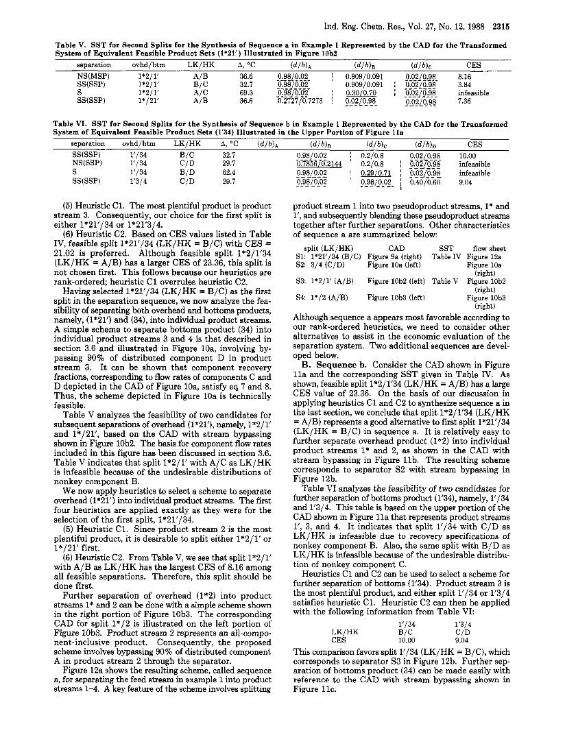
Table V. SST for Second Splits for the Synthesis of Sequence a in Example 1 Represented by the CAD for the Transformed System of Equivalent Feasible Product Sets (1*21’) Illustrated in Figure 10b2

separation ovhd/btm LK/HK A, “C ( d / b ) A ( d l b h ( d l b ) , CES

36.6 --- 0.98l0.02 ---- 0.909/0.091 oLO>~~.l~- 8.16 32.7 --- 0.9810.02 ---- 0.909/0.091 i _010_210_._98 3.84

NS(MSP) 1*2/1‘ AIB SS(SSP) 1*2/1‘ B/C S 1*2/1’ A/C SS(SSP) 1*/21‘ A/B

0.981_0._02 I 0.30/0.70 I -OL?2&9>- infeasible 69.3 --_ 36.6 0.272710.7273 j -- 0.0210.9_8_ - --- 0.02~0,98_ 7.36

Table VI. SST for Second Splits for the Synthesis of Sequence b in Example 1 Represented by the CAD for the Transformed System of Equivalent Feasible Product Sets (1’34) Illustrated in the Upper Portion of Figure l la

separation ovhd/btm LK/HK A, “ C ( d / b ) A ( d / b ) B (d1b)c ( d l b ) , CES

B/C 29.7 0.7856/0.2144 0.2/0.8 I _O,Oy_OXj infeasible SS(SSP) 1’/34

S 1’134 BID 62.4 -- 0.98JjLOz I 0.29/0.71 I _O,O2J_ol9S infeasible SS(SSP) 1‘314 C/D 29.7

32.7 - 0.98l@z -- j 0.2/0.8 , gq0,9_8_ 10.00 NS(SSP) 1’134 C/D

0.98/0.02 I 0.40/0.60 9.04 --- ---- 0.98/0.02 ’ __ - - - -

(5) Heuristic C1. The most plentiful product is product stream 3. Consequently, our choice for the first split is either 1*21’/34 or 1*21’3/4.

(6) Heuristic C2. Based on CES values listed in Table IV, feasible split 1*21’/34 (LK/HK = B/C) with CES = 21.02 is preferred. Although feasible split 1*2/1‘34 (LK/HK = A/B) has a larger CES of 23.36, this split is not chosen first. This follows because our heuristics are rank-ordered; heuristic C1 overrules heuristic C2.

Having selected 1*21’/34 (LK/HK = B/C) as the first split in the separation sequence, we now analyze the feasibility of separating both overhead and bottoms products, namely, (1*21’) and (34), into individual product streams. A simple scheme to separate bottoms product (34) into individual product streams 3 and 4 is that described in section 3.6 and illustrated in Figure loa, involving bypassing 90% of distributed component D in product stream 3. I t can be shown that component recovery fractions, corresponding to flow rates of components C and D depicted in the CAD of Figure loa, satisfy eq 7 and 8. Thus, the scheme depicted in Figure 10a is technically feasible.

Table V analyzes the feasibility of two candidates for subsequent separations of overhead (1*21’), namely, 1*2/ 1’ and 1*/21’, based on the CAD with stream bypassing shown in Figure 10b2. The basis for component flow rates included in this figure has been discussed in section 3.6. Table V indicates that split 1*2/1’ with A/C as LK/HK is infeasible because of the undesirable distributions of nonkey component B.

We now apply heuristics to select a scheme to separate overhead (1*21’) into individual product streams. The fiit four heuristics are applied exactly as they were for the selection of the first split, 1*21’/34.

(5) Heuristic C1. Since product stream 2 is the most plentiful product, it is desirable to split either 1*2/1’ or 1*/21’ first.

(6) Heuristic C2. From Table V, we see that split 1*2/1’ with A/B as LK/HK has the largest CES of 8.16 among all feasible separations. Therefore, this split should be done first.

Further separation of overhead (1*2) into product streams 1* and 2 can be done with a simple scheme shown in the right portion of Figure 10b3. The corresponding CAD for split 1*/2 is illustrated on the left portion of Figure 10b3. Product stream 2 represents an all-component-inclusive product. Consequently, the proposed scheme involves bypassing 90% of distributed component A in product stream 2 through the separator.

Figure 12a shows the resulting scheme, called sequence a, for separating the feed stream in example 1 into product streams 1-4. A key feature of the scheme involves splitting

product stream 1 into two pseudoproduct streams, 1* and l’, and subsequently blending these pseudoproduct streams together after further separations. Other characteristics of sequence a are summarized below:

S1: 1*21’/34 (B/C) Figure 9a (right) Table IV Figure 12a S2: 314 (C/D) Figure 10a (left) Figure 10a

S3: 1*2/1’ (A/B) Figure 10b2 (left) Table V Figure 10b2

S4: 1*/2 (A/B) Figure lob3 (left) Figure 10b3

Although sequence a appears most favorable according to our rank-ordered heuristics, we need to consider other alternatives to assist in the economic evaluation of the separation system. Two additional sequences are developed below.

B. Sequence b. Consider the CAD shown in Figure l l a and the corresponding SST given in Table IV. As shown, feasible split 1*2/1’34 (LK/HK = A/B) has a large CES value of 23.36. On the basis of our discussion in applying heuristics C1 and C2 to synthesize sequence a in the last section, we conclude that split 1*2/1’34 (LK/HK = A/B) represents a good alternative to first split 1*21’/34 (LK/HK = B/C) in sequence a. I t is relatively easy to further separate overhead product (1*2) into individual product streams 1* and 2, as shown in the CAD with stream bypassing in Figure l l b . The resulting scheme corresponds to separator S2 with stream bypassing in Figure 12b.

Table VI analyzes the feasibility of two candidates for further separation of bottoms product (1’34), namely, 1’/34 and 1’3/4. This table is based on the upper portion of the CAD shown in Figure l l a that represents product streams l’, 3, and 4. I t indicates that split 1’/34 with C/D as LK/HK is infeasible due to recovery specifications of nonkey component B. Also, the same split with B/D as LK/HK is infeasible because of the undesirable distribution of nonkey component C.

Heuristics C1 and C2 can be used to select a scheme for further separation of bottoms (1’34). Product stream 3 is the most plentiful product, and either split 1’/34 or 1’3/4 satisfies heuristic C1. Heuristic C2 can then be applied with the following information from Table VI:

split (LK/HK) CAD SST flow sheet

(right)

(right)

(right)

1’134 1‘3/4 C/D 9.04

LK/HK B/C CES 10.00

This comparison favors split 1’/34 (LK/HK = B/C), which corresponds to separator S3 in Figure 12b. Further separation of bottoms product (34) can be made easily with reference to the CAD with stream bypassing shown in Figure l lc .


Table VII. SST for Second Splits for the Synthesis of Sequence c in Example 1 Represented by the CAD for the Transformed System of Equivalent Feasible Product Sets (21’34) Illustrated in Figure 1 la

separation obhd/btm LK/HK A, “C ( d / b ) A (d /b)B ( d / b ) c (d /b )D CES -

SS(SSP) 21’3/4 C/D 29.7 &98J_o._O2 _O.j@lp,O_Z_ _O?_S/_o,O_2- I 0.4/0.6 6.13 32.7 -OL9jL0,0_Z- _OL9jlQ.Gz 0.2/0.8 I 0.0018/0.9982 22.84 62.4 0.98/0.02 0.98/0.02 I 0.295/0.705 1 0.02j0.98 infeasible

NS(SSP) 21’/34 C/D 29.7 -O.j8J~.o_2- 0.79/0.21 0.2/0.8 - 0.02j0.98 - - - - - - 43.62

SS(SSP) 21’/34 B/C S 21‘/34 B/D - - - - - - - - - - - - - I - - - - - -

Table VIII. SST for First Sulits in ExamDle 2A boresented by the CAD of Figure 15 separa- ovhdl LKI A,

SS(MSP) 12/34567 B/C 11.3 0.942/0.058 0.06/0.94 3.114 SS(MSP) 123/4567 C/D 28.3 0.99/0.01 0.975/0.025 I 0.025/0.975 0.01/0.99 12.367 SS(MSP) 1234/567 D/E 8.2 0.845/0.155 I 0.155/0.845 9.079 SS(MSP) 12345/67 E/F 13.2 0.99/0.01 0.975/0.025 I 0.025/0.975 0.01/0.99 0.005/0.995 9.660 SS(MSP) 123456/7 G / J 13.6 0.9/0.1 0.8/0.2 0.701/0.299 I 0.3/0.7 0.2/0.8 0.1/0.9 0.1/0.9 7.440

(comp. G)

To summarize, key features of sequence b shown in Figure 12b are

split (LK/HK) CAD SST S1: 1*2/1’34 (A/B) Figure l l a Table IV S2: 1*/2 (A/B) Figure l l b S3: 1’/34 (B/C) Figure l l a (upper portion) Table VI S4: 3/4 (C/DI Figure l l c

C. Sequence c. A third separation sequence can be synthesized with reference to the CAD of Figure l l a and the corresponding SST of Table IV. Among all feasible splits listed in the table, split 1*/21’34 (LK/HK = A/B) has the next lower CES value of 6.22, compared to those of splits 1*2/1’34 (LK/HK = A/B) and 1*21’/34 (LK/HK = B/C). The latter two splits correspond to separator S1 in sequences a (Figure 12a) and b (Figure 12b), respectively.

Starting with split 1*/21’34 (LK/HK = A/B), the subsequent separation scheme can be constructed by considering part of the CAD of Figure l l a that represents product streams 2, l’, 3, and 4. Table VI1 analyzes the feasibility of two candidates for further separation of the bottoms 21’3/4 and 21’/34. Both splits involve removing the most plentiful product stream, 3, early as specified by heuristic C1. Table VI1 indicates that split 21‘/34 (LK/ HK = B/D) is infeasible because of the undesirable distribution of nonkey component c. By comparing CES values listed in the table, we conclude that feasible split 21’/34 (LK/HK = C/D) is preferred over other options. The resulting separation scheme, sequence c, is shown in Figure 12c and can be summarized as follows:

split (LK/HK) CAD SST S1: 1*/21’34 (A/B) Figure l l a Table IV S2: 21’/34 (C/D) Figure l l a Table VI1 S3: 2/1’ (B/C) 54: 314 (C/D)

The preceding solutions to example 1 include four separators. The latter number is one more than the apparent minimum number of separators, Smin, required for our problem that is specified by the following equation (Bam- opoulos, 1984; Cheng, 1987):

S,,, = min (C,P) - 1 = min (4,4) - 1 = 4 - 1 = 3 (21)

In the equation, C is the number of components and P is the number of product streams. An initial sequence in-

(comp. J)

corporating only a minimum number of separators often requires the use of sharp separators alone, or the combined use of both sharp and sloppy separators. The need for four separators in our solution results from our restriction of using sloppy separators only. This restriction is justified by the practical need to synthesize several good initial sequences having at most one more separator than other competing sequences with a minimum number of separators.

Actually, our synthesis method can be easily extended to generate equally good initial sequences with possibly three different types of separators, namely, all-sharp, all-sloppy, and both sharp and sloppy (Le., mixed) separators. This extension is possible because our problem representation by the CAD and our rank-ordered heuristics are readily applicable to both sloppy and sharp separations. Additional details can be found in Cheng and Liu (1988).

5.2. Example 2A: Fractionation of Refinery Light Ends. Example 2A corresponds to the fractionation of 13 refinery light-end components into 7 products (Tedder, 1984). Data for feed and product streams are specified in Appendix A. Figure 15 shows a CAD representing this example, and Table VI11 presents an SST for candidates of first splits depicted on the figure. Both the CAD and SST indicate that this fractionation problem consists of many sloppy splits and distributed nonkey components. Normally, we need to carry out a feasibility analysis of product splits based on component recovery specifications and nonkey component distributions as discussed in sections 3.2-3.4. However, for practical purposes, we can assume that each sloppy split is feasible and distributed nonkey components are allowed to be present in product streams. Our assumption is justified by a distinct feature of the fractionation problem in that most products are to be used as fuel streams and they are blended together later for burning. This assumption has also been incorporated in the work by Tedder (1984).

The heuristic synthesis of separation sequences can be done with reference to the SST of Table VIII.

(1) Heuristic M1. Normal boiling point differences (As) are large enough to use ordinary distillation.

(2) Heuristic M2. Refrigeration operated at high pressure is needed to distill off components of low boiling points.

(3) Heuristic S1. Not applicable. (4) Heuristic S2. Perform splits 1234/567 and 12/34567

last due to their small ATs of 8.2-11.3 “C. ( 5 ) Heuristic C1. Not applicable since none of the

product streams represent a large fraction of the feed.


we note the following comparison: 1/23 1213

11.3 AT, OC 30.2 CES 11.65 6.13

Split 12/3 represents a relatively difficult separation with a small AT (heuristic S2), and it has a lower CES of 6.13 (heuristic C2). Therefore, split 1/23 is preferred.

For separating bottoms (4567), we avoid performing split 4/567 early in the sequence because of the small AT of 8.2 OC (heuristic S2). The remaining options to be chosen are compared below:

B/C LKjHK A P

45/67 45617 GIJ LK/HK E/F

CES 5.45 18.27

We choose split 456/7 first according to heuristic C2. This gives an overhead of (456) and a bottoms of product stream 7. A good split to further separate overhead (456) is split 45/6, since it can be shown that this split has a larger CES value than split 4/56. The resulting separation sequence, called sequence a, is illustrated in Figure 13a.

By following the preceding procedure, it is fairly easy to synthesize other sequences for this problem. For example, parts b and c of Figure 13 show two alternative sequences, called sequences b and c, that have also been found by Tedder (1984). Sequence b is constructed by starting with the first split 123456/7 with a CES of 7.440 (see Table VIII); sequence c is synthesized with an initial split 1234/567, having a CES of 9.079. Finally, based on CES values listed in Table VIII, it is obvious that another sequence can be synthesized by starting with an initial split 12345/67 with a larger CES of 9.680.

5.3. Example 2B: Fractionation in Refinery Satu- rates-Gas Plant. This example, taken from Watkins (1979), is included here to demonstrate the effectiveness of the heuristic method by comparing the resulting separation sequences with reported industrial sequences. I t involves the fractionation of 14 refinery saturates-gas components (labeled X, A, B, ..., L, M) into 9 product streams (denoted by 0, 1 , 2 , ..., 8). The problem represents a slight modification of example 2A. Data for feed and product streams are specified in Appendix A and represented by the CAD of Figure 16.

Table IX shows an SST for candidates of first splits depicted in the CAD of Figure 16. Based on CES values listed in the table, the following three initial splits are favored by heuristic C2: (1) 01234567/8, CES = 28.160; (2) 0123456/78, CES = 6.061; and (3) 0123/45678, CES = 3.459. By starting with these initial splits and applying rank-ordered heuristics to determine subsequent splits, it is relatively easy to synthesize three separation sequences, called sequences a-c, as shown in Figure 14a-c.

5.4. Cost Evaluations of Separation Sequences. Total annual costs of separation sequences a-c for each example problem have been estimated after rigorous flow-sheet simulations by DESIGN I1 (ChemShare Cor- poration, 1985). Detailed costing data are specified in Appendix B, and resulting costs in $1000/year (first quarter of 1987) are summarized in Table X.

For example 1, the cost ranking of sequences a-c is not in the same order of proposed sequences (ranking of sequences b and c is reversed). We attribute this result to the fact that various degrees of sloppiness and different extents of bypassing are involved in different sequences. Also, we note that costs of sequences a-c differ by only a few percent. As was suggested by Tedder (1975), the magnitude of possible round-off errors (noises) resulting

13.6 AT, “C 13.2

n

- Sl 2

3

Figure 12. Flow sheets of separation sequences synthesized for example 1 (a, top) Sequence a. (b, middle) Sequence b. (c, bottom) Sequence c.

(6) Heuristic C2. Split 123/4567 has the largest CES of 12.367 and should be done first. This split gives an overhead of (123) and a bottoms of (4567).

To select a scheme to further separate overhead (123),


12314557 {

' 234 / 1214 56' ( S 4 )

5 6 1 ( S i ) \

1 5 6 , < ( S O

f 5 3 ) 7

Figure 13. Flow sheets of separation sequences synthesized for example 2A. (a, top) Sequence a. (b, middle) Sequence b. (c, bottom) Sequence c.

from the application of optimization techniques to multicomponent separation-sequencing problems with different initial conditions could often be greater than the cost difference indicated in Table X. Under such situa- tions, it is important to select the best sequence from several initial sequences based on additional performance criteria other than the total annual cost, such as the ease

0121456178

(Sl)

Figure 14. Flow sheets of separation sequences synthesized example 2B. (a, top) Sequence a. (b, middle) Sequence b. bottom) Sequence c.

for (C,

of startup and shutdown, operational safety considerations, etc. The heuristic method presented in this work provides a simple and effective procedure for the systematic synthesis of good initial sequences for such a multiobjective design optimization.

For example 2A, the cost ranking is identical with the order of proposed sequences. However, Tedder (1984)


Table IX. SST for First Solits in Examole 2B boresen ted by the CAD of Figure 16

separation

SS(MSP) SS(MSP) SS(MSP) SS(MSP) SS(MSP) SS(MSP) SS(MSP) SS(MSP)

ovhdjbtm 0/123456378 01/2345678 012/345678 0123/45678 01234/5678 012345/678 0123456/78 01234567/8

LK/ HK

XIB -

A.

AjB B/C

D I E EIF

30.2

C i D

96.6

same as 12/34567 in Table VI11 same as 123/4567 in Table VI11 same as 1234/567 in Table VI11 same aa 12345/67 in Table VI11 same as 123456/7 in Table VI11

0.975/0.025 0.975/0.025 j 0.006/0.994

(d/b)HHKz ( ~ / ~ ) H H K B CES 0.532 1.572 1.126 3.459 2.572 2.380 6.061

28.160

Table X. Costs of Separat ion Sequences in Illustrative Examples (in $1000/Year, First Quarter of 1987) sevar ator

s1 s 2 s3 s 4 s5 S6 57 sa total

sequence a 1330 649 434 70 2487 sequence b 1033 227 687 650 2597 sequence c 464 1095 290 649 2498

sequence a 594 191 370 292 320 262 2029 sequence b 784 338 268 292 320 262 2264 sequence c 971 260 321 229 292 228 2301

example 1

example 2A

example 2B sequence a 5599 861 225 370 92 292 262 320 8021 sequence b 5202 537 225 320 92 292 262 850 7780 sequence c 3816 225 2702 92 292 370 262 320 8079

Table XI. Summary of Reported Studies on the Synthesis of Sloppy Multicomponent Separation Sequences investigator

Bamopoulos (1984); Nath (1977) Sophos (1981) Bamopoulos et al. (1988) Tedder (1984)

1. consideration of sloppy

2. problem representation

3. feasibility analysis of

splits

sloppy splits

4. means for ranking sequences other than costing

5. remarks

yes

MAD"

not considered

by CDSb

no (sharp splits only) yes

MAD MAD and component recovery matrix

without nonkey components

considered for a binary feed

by the mass load of by heuristics separation

only an "optimum" sequence both sloppy and sharp is developed; no near separators are used; optimum sequences are restrictions are imposed on given the types of sloppy

separators; also consider one-section separators (rectifiers or strippers) and sinele-stane flash units

all candidates of "optimum" sequences are developed; a modified MAD is used

yes

mass/energy balance equations

not considered

costing only

complex columns are considered by a combined heuristidynamic programming method

investigator Muraki and Hayakawa (1984);

Muraki et al. (1986) Floudas (1987) Muraki and Havakawa (1987) Muraki and Havakawa (1988) 1. consideration of sloppy

2. problem representation

3. feasibility analysis of

4. means for ranking

split

sloppy splits

sequences other than costing

5. remarks

~~

no

MAD and mass/energy balance equations

by an objective function

an evolutionary search is used to improve the objective function for each sequence, whose mass flow rates are assigned by a modified MAD

no

mass/energy balance equations

by an objective function

all sharp configurations are embedded in a superstructure; die optimum sequence is obtained by a mathematical programming method

yes


not considered

costing only

an-optimization technique is used to solve for the best sequence

yes


not considered

costing only

key component recoverless are treated as design variables of an optimization problem for a specific separation sequence; use an evolutionary approach to compare costs of neighboring sequences

a Material allocation diagram. *Coefficient of difficulty of separation.

found that sequence b was slightly cheaper than sequence a. This discrepancy may be due to some differences in the methods used to establish column pressures in both studies.

Table X shows that the cheapest sequence for example 2B is sequence b. Considering the fact that costs of se-

quences a and c are higher than that of sequence b by only 3.1% and 3.8%, respectively, we conclude that these sequences are all good initial sequences. Most importantly, when comparing costs of sequences a-c ($7 780 0001 to $8079000/year) with that ($9257OOO/year) of the cheapest industrial sequence reported in Watkins (1979)) significant


Table XII. Similarities between the Synthesis of Multicomponent Separation Sequences and the Synthesis of Heat-Exchanger Networks

multicomDonent seDaration seauences heat-exchanger networks 1. graphical representation of the synthesis problem and

its related table analysis e.g., by component assignment diagram and its related separation specification table

a. product-split feasibility analysis b. transformation of infeasible product seta due to component recovery specifications and nonkey component distributions by stream splitting and/or bypassing

a. a priori target of the most probable, minimum number of separators (Bamapoulos, 1984; Cheng, 1987) b. reducing the number of separators by using both sloppy and sharp splits (Cheng, 1987) c. minimizing separation utility consumptions by using balanced separators (50/50 split) and other heat-integration schemes

2. feasibility analysis

3. achieving synthesis goals

Table XIII. Suecification of Example 2A0

e.g., by temperature-interval diagram and its related problem table

a. heat-exchange feasibility analysis b. transformation of infeasible heat exchanges due to minimum

approach-temperature constraint by stream splitting and/or bypassing

a. a priori target of the most probable, minimum number of heat-exchange units (exchangers, heaters and/or coolers)

b. reducing the number of heat-exchange units by stream splitting and bypassing

c. minimizing heating and cooling-utility consumptions by stream splitting and bypassing

product flow rates, mol/h normal feed flow components bp, "C rate, molih 1 2 3 4 5 6 7 A. C3 -42.1 121.19 118.08 3.11 B. i-C,, -11.8 59.58 1.47 54.63 2.88 0.60 C. n-C, -0.5 116.84 1.47 5.77 109.60 2.99 D. i-C, 27.8 59.96 1.50 49.20 8.68 0.58 E. n-C6 36.1 62.69 0.63 9.08 51.43 1.55 F. o-CS 49.2 32.51 0.81 28.53 G. 22DMB 49.7 6.63 0.07 5.25 H. 23DMB 58.0 10.81 0.05 7.53 I. 2MEP 60.3 62.72 18.82 J. 3MEP 63.3 39.61 7.92 K. n-C6 68.7 80.33 8.02 L. C& 80.1 23.91 2.39 M. '27' 176.7 7.37

(I 22DMB = 2,2-dimethylbutane; 23DMB = 2,3-dimethylbutane; 2MEP = 2-methylpentane; 3MEP = 3-methylpentane.

3.17 1.31 3.23

43.90 31.69 72.31 21.52

7.37

Figure 15. CAD for example 2A.

savings result from our proposed sequences:

6. Concluding Remarks The present work proposes a simple and practical ap-

proach to the systematic development of initial sequences of sloppy multicomponent separation sequences. Included in the work are problem representation, feasibility analysis, heuristic synthesis, and illustrative examples. Table XI summarizes the key features of reported studies on the synthesis of sloppy multicomponent separation sequences.

We have developed a new problem representation, called the component assignment diagram (CAD), for conven- iently synthesizing separation sequences to yield sloppy product sets, in which some components may simultane-

Figure 16. CAD for example 2B.

ously appear in two or more product streams. The CAD allows different kinds of product sets to be easily visual- ized. It also permits some complex synthesis problems to be clearly elucidated. An example of such problems is the multiple-split-point (MSP) sloppy separation, illustrated in Figure 3c and included in examples 2A and 2B. Our problem representation by the CAD is similar to the use of temperature-interval diagram, an on-diagram-oriented method widely used in heat-exchanger network (HEN) synthesis (Liu, 1987).

The CAD is a simpler representation of the sloppy separation problem than an alternative representation called the material allocation diagram (MAD) proposed by Nath (1977) and used by a number of subsequent in-


Institute of Technology for many helpful discussions on the sloppy separation problem and to Diane S. Cannaday and Marie Hetherington for their assistance in the prep- aration of this manuscript.

Nomenclature

A = cross-sectional area of distillation column, m2 b = component molar flow rate in the bottoms product, mol/h;

or in normalized situation, component recovery fraction in the bottoms product, dimensionless

B = molar flow rate of the bottoms product, mol/h C = number of components CAD = component assignment diagram CES = coefficient of ease of separation defined in eq 20 C,, = unit cost of cooling utility, $/h C,, = unit cost of heating utility, $/h d = component molar rate in the overhead product, mol/h;

or in normalized situation, component recovery fraction in the overhead product, dimensionless

D = molar flow rate of the overhead product, mol/h D, = column diameter, m, eq B.l ( d / b ) , = split or distribution ratio of component i, that is, the

ratio of recovery fraction of component i in the overhead to that in the bottoms, dimensionless

f = D/B or B/D, whichever is smaller than or equal to unity, dimensionless

H, = height of the distillation column, m HHK = heavier-than-heavy key components or heavy com-

HHK1-3 = heavy components whose volatilities are in a de-

HK = heavy-key component Ki = vapor-liquid equilibrium ratio of component i, dimen-

LK = light-key component LLK = lighter-than-light key components or light components LLK1-3 = light components whose volatilities are in an as-

N = number of theoretical stages, dimensionless nil = molar flow rate of component i in product j , mol/h Nmin = minimum number of theoretical stages P = number of product streams; or column pressure, Pa Qc = condenser duty, W or J / h QR = reboiler duty, W or J / h R D = external or operating reflux ratio RD,min = minimum reflux ratio RD!, = total reflux Smin = apparent minimum number of separators, eq 21 SST = separation specification table T = normal boiling point, 'C T D = dew point of the vapor stream at the column top, 'C,

U = overall heat-transfer coefficient, W/(m2.'C) V = average vapor velocity, m/h, eq B.l z, = mole fraction of component i in the feed, dimensionless Greek Letters aLK,HK = relative volatility of LK with respect to that of HK a, = relative volatility of component i with reference to that

7 = overall stage efficiency, assumed to be 0.8

Symbol h = AT = (normal boiling point difference, 'C)1.8, or 1OO(a

- 1)

ponents

scending order

sionless

cending order

eq B.2

of HK

Table XIV. Unit Costs of Heating and Cooling Utilities available pressure,

utility temp, O C Pa cost, $/lOBJ steam steam steam steam steam cooling water propylene propylene freon

115.0 130.6 185.6 231.1 281.1 35.0 4.4

-17.8 -106.7

68 932 5.414 275728 7.396

1033 980 10.036 2 757 280 13.294 6 445 142 16.610

0.145 2.765 7.261 9.479

vestigators. In an MAD, components are represented by rectangles of fixed height and of width proportional to their concentration. The rectangles are arranged in order of decreasing volatility or separation factor and are separated by dashed lines; the desired products are separated by solid lines. The CAD is free of many cumbersome diagram- matical manipulations that are frequently required to make an MAD more recognizable.

We have also proposed a separation specification table (SST) to aid in the analysis of technical feasibility of product splits. This analysis identifies technically infeasible splits resulting from component recovery specifications and nonkey component distributions. The SST is a useful tool to properly define and specify key and nonkey components, quickly identify feasible and infeasible product splits, and systematically consider sloppy separations with multiple distributed components. By comparing results from rigorous simulations with those from shortcut modeling by the Fenske equation, we have identified some quantitative guidelines for applying the Fenske equation to estimate nonkey component distributions.

As described in this work, feasibility aspects of product splits are in many ways similar to those of HEN synthesis. For example, the analysis of product-split feasibility corresponds to the determination of heat-exchange feasibility (due to the minimum approach-temperature constraint). Likewise, the transformation of infeasible splits into equivalent feasible splits is analogous to the use of stream splitting and/or bypassing to avoid the minimum approach-temperature violations for infeasible heat exchanges. Table XI1 lists other similarities between the synthesis of sloppy multicomponent separation sequences and the HEN synthesis.

Our synthesis method involves two key steps. First, the feasibility of product splits shown on a CAD is assessed with the aid of an SST. Next, several separation sequences are specified by applying six rank-ordered heuristics. As demonstrated by illustrative examples, the proposed heuristic method offers a simple and effective procedure for design engineers to generate a number of initial of initial sequences for sloppy multicomponent separations. These initial sequences represent good candidates for the detailed flow-sheet optimization. Finally, we note that our method has been implemented in an expert system using TURBO PROLOG on a personal computer (Rony, 1987).

Acknowledgment

The authors express their appreciation to the Depart- ment of Chemical Engineering and Computing Center a t VPI and SU for providing financial support and computer time for this work and to the ChemShare Corporation, Houston, T X and the Aspen Technology, Inc., Cambridge, MA, for the use of their computer-aided design packages, DESIGN I1 and ASPEN PLUS. Special thanks are extended to Professor D. William Tedder of the Georgia

Appendix A: Problem Specification Three example problems are presented in this work, and

their specifications are given below. Example 1: Separation of Light Hydrocarbons by

Ordinary Distillation. This example involves the sep-


aration of a four-component mixture of light hydrocarbons by ordinary distillation (Nath, 1977). The feed mixture is

A: n-butane (nC,) 25 -0.5 component" mol/h normal bp, T , "C AT, "C

36.6 32.7 29.7

B: n-pentane (nC6) 25 36.1 C: n-hexane (nCs) 25 68.7 D: n-heptane (nC,) 25 98.4

I t is desired to separate the feed into the following four product streams:

desired product streams A B C D mol/h

component mole fraction

1 0.4615 0.3846 0.1539 32.5 2 0.4444 0.5556 22.5 3 0.6667 0.3333 30.0 4 1.0000 15.0

Example 2A Fractionation of Refinery Light Ends. This example problem involves the fractionation of 13 refinery light-ends components into 7 product streams (Tedder, 1984). I t is a modified version of example 2B given below as originally reported by Watkins (1979). The feed mixture and product specifications are listed in Table XIII, and the CAD for represting the problem is given in Figure 15.

Fractionation in Refinery Satu- rates-Gas Plant. This example is taken from Watkins' book (1979) and is essentially the same as example 2A. The exception is that one extra light component, X (C2H6), with a normal boiling point of -88.6 "C, appears in the feed and two additional product streams (labeled 0 and 8) are t~ be separated. For simplicity, this problem is represented by a CAD shown in Figure 16.

Appendix B: Distillation Costing Data

column diameter

Example 2B:

A. Column Cost (Rathore et al., 1974).

(1 + R,)D(TD + 273) VP (B.1) Dc = 1.7057

column height

03.2)

where V is the average vapor velocity (m/h) as given by

(B.3)

total installed column cost ($COL) (Peters and Timmer- haus, 1980)

N Hc = 0.61- + 4.27 17

1 V 25.31- P

1 803.7(CE Index, 1987) 599.4(CE Index, 1979)

(B.4)

$COL = 4263.67Dc'.'292H

B. Reboiler Cost (Guthrie, 1969). Assume that U = 766.3 W/(m2-OC) (135 Btu/(h-ft2.OF)). total installed reboiler cost ($RINS)

] (B.5) 803.7(CE Index, 1987)

$RINS = 1613*52A0'65 274.O(CE Index, 1969)

reboiler operating cost ($ROP) $ROP = (8500 h/year)Cu,+QR + 0.02($RINS)

= 624.4 W/(m2."C) (110 Btu/(h.ft2.0F)).

(B.6) C. Condenser Cost (Guthrie, 1969). Assume that U

total installed condenser cost ($CINS)

] 03.7) 803.7(CE Index, 1987) 274.O(CE Index, 1969)

$GINS = 1613.52A0.65

total condenser operating cost ($COP) $COP = (8500 h/year)C,,QR + 0.02($CINS)

Utility (C,,,). See Table XIV.

10-year project life is assumed.

(B.8) D. Unit Costs of Heating Utility (C,,+) and Cooling

E. Total Annual Cost ($TAC). Costing basis: A

$COL + $RINS + $CINS 10

$TAC = $ROP + $COP + (B.9)

Literature Cited

Louis, MO, 1984. Bamopoulos, G. Ph.D. Dissertation, Washington University, St.

Bamopoulos, G.; Nath, R.; Motard, R. L. AZChE J. 1988, 34, 763. ChemShare Corporation "DESIGN I1 User's Guide"; Houston, TX,

1985. Cheng, S. H. Ph.D. Dissertation, Virginia Polytechnic Institute and

State University, Blacksburg, VA, 1987. Cheng, S. H.; Liu, Y. A. "Studies in Process Design and Synthesis:

Part IX. A Unifying Framework for Multicomponent Separation Sequencing with Sloppy Product Streams". Symposium on Pro- cess Synthesis, AIChE Annual Meeting, Washington, DC, Nov 1988.

Coulson, J. M.; Richardson, J. F.; Backhurst, J. R.; Harker, J. H. Chemical Engineering, Vol. 2, Unit Operations; Pergamon: Ox- ford, United Kingdom, 1980.

Douglas, J. M.; Malone, M. F.; Doherty, M. F. Comput. Chem. Eng. 1985, 9, 447.

Fenske, M. R. Ind. Eng. Chem. 1932,24, 482. Floudas, C. A. AZChE J. 1987,33, 540. Guthrie, K. M. Chem. Eng. 1969, 76(6), 114. Henley, E. J.; Seader, J. D. Equilibrium-Stage Separation Opera-

tions in Chemical Engineering; Wiley: New York, 1981. King, C. J. Separation Processes, 2nd ed.; McGraw-Hill: New York,

1980. Liu, Y. A. In Recent Developments in Chemical Process and Plant

Design; Liu, Y. A., McGee, H. A., Jr., Epperly, W. R., Eds.; Wiley: New York, 1987; pp 147-260.

Muraki, M.; Hayakawa, T. J . Chem. Eng. Jpn . 1984,17, 533. Muraki, M.; Hayakawa, T. J . Chem. Eng. Jpn. 1987,20, 195. Muraki, M.; Hayakawa, T. Chem. Eng. Sci. 1988,43, 259. Muraki, M.; Katoaka, K.; Hayakawa, T. Chem. Eng. Sci. 1986,41,

Nadgir, V. M.; Liu, Y. A. AZChE J. 1983,29, 926. Nath, R. Ph.D. Dissertation, University of Houston, Houston, TX,

Nath, R.; Motard, R. L. AIChE J. 1981,27, 321. Peters, M. S.; Timmerhaus, K. D. Plant Design and Economics for

Chemical Engineers, 3rd ed.; McGraw-Hill: New York, 1980. Rathore, R. N. S.; Van Wormer, K. A.; Powers, G. J. AZChE J . 1974,

20, 491, 940. Rony, K. E. "SSG: Sloppy Separation Generator-A Turbo Prolog

Expert System". Senior Research Report, 1987; Chemical Engi- neering, Virginia Polytechnic Institute and State University, Blacksburg, VA.

1843.

1977.

Seader, J . D.; Westerberg, A. W. AZChE J. 1977,23, 951. Sophos, A. Ph.D. Dissertation, University of Minnesota, Minneapo-

lis, MN, 1981. Stupin, W. J.; Lockhart, F. J. "The Distribution of Nonkey Com-

ponents in Multicomponent Distillation". AIChE Annual Meet- ing, Los Angeles, CA; 1968.

Tedder. D. W. Ph.D. Dissertation. Universitv of Wisconsin. Madison, WI, i975.

Tedder, D. W. "The Synthesis of Optimal Gas Saturates Separation

Watkins, R. N. Petroleum Refinery Distillation, 2nd ed.; Gulf

Westerberg, A. W. Comput. Chem. Eng. 1985, 9, 421.

System". AIChE Annual Meeting, San Francisco, CA, 1984.

Houston, 1979.

Received for review February 26, 1988 Revised manuscript received July 11, 1988

Accepted July 31, 1988

studies in chemical process design and synthesis. a ...€¦ · masoneilan handbook for control...

Documents