Helsinki University of Technology Laboratory of Acoustics and Audio Signal Processing

Espoo 2005 Report 74

STUDIES ON AUDITORY PROCESSING OF SPATIAL SOUND AND SPEECH BY NEUROMAGNETIC MEASUREMENTS AND COMPUTATIONAL MODELING

Kalle Palomäki

Helsinki University of Technology Laboratory of Acoustics and Audio Signal Processing

Espoo 2005 Report 74

STUDIES ON AUDITORY PROCESSING OF SPATIAL SOUND AND SPEECH BY NEUROMAGNETIC MEASUREMENTS AND COMPUTATIONAL MODELING

Kalle Palomäki

Dissertation for the degree of Doctor of Science in Technology to be presented with due permission for public examination and debate in Auditorium S4, Department of Electrical and Communications Engineering, Helsinki University of Technology, Espoo, Finland, on the 17th of June 2005, at 12 o'clock noon.

Helsinki University of Technology

Department of Electrical and Communications Engineering

Laboratory of Acoustics and Audio Signal Processing

Teknillinen korkeakoulu

Sähkö- ja tietoliikennetekniikan osasto

Akustiikan ja äänenkäsittelytekniikan laboratorio

Helsinki University of Technology

Laboratory of Acoustics and Audio Signal Processing

P.O. Box 3000

FIN-02015 HUT

Tel. +358 9 4511

Fax +358 9 460 224

E-mail lea.soderman@hut.fi

ISBN 951-22-7716-6 ISSN 1456-6303

Otamedia Oy

Espoo, Finland 2005

HELSINKI UNIVERSITY OF TECHNOLOGYP.O. BOX 1000, FI-02015 TKK

http://www.tkk.fi

ABSTRACT OF DOCTORAL DISSERTATION

Author

Name of the dissertation

Date of manuscript Date of the dissertation

Monograph Article dissertation (summary + original articles)

Department

Laboratory

Field of research

Opponent(s)

Supervisor

(Instructor)

Abstract

Keywords

Number of pages ISBN (printed)

ISBN (pdf) ISBN (others)

ISSN (printed) ISSN (pdf)

Publisher

Print distribution

The dissertation can be read at http://lib.tkk.fi/Diss/

1

This thesis was done in collaboration with the following units:

Laboratory of Acoustics and Audio Signal Processing, Helsinki University of Technology, Finland

Apperception & Cortical Dynamics (ACD), Department of Psychology, University of Helsinki, Finland

Speech and Hearing, Department of Computer Science, University of Sheffield, United Kingdom

BioMag Laboratory, Engineering Centre, Helsinki University Central Hospital, Helsinki, Finland

2

Acknowledgements This thesis was undertaken at the Laboratory of Acoustics and Audio Signal Processing at the Helsinki University of Technology in collaboration with the Department of Computer Science in the University of Sheffield, Apperception and Cortical Dynamics, Department of Psychology at the University of Helsinki and BioMag laboratory of the Helsinki University Central Hospital. I wish to thank Prof. Paavo Alku, Doc. Hannu Tiitinen, Dr. Guy Brown, and Doc. Patrick May for their supervision as well as their research efforts in studies in the thesis. I am grateful to Ville Mäkinen, Dr. Jon Barker, and Prof. DeLiang Wang for their participation in the studies in this thesis. Many thanks for Prof. Martin Cooke and Prof. Kimmo Alho for their efforts in pre-examination of the thesis. For Dr. Aki Härmä, Prof. Matti Karjalainen, and Prof. Unto Laine, I am especially grateful as they arranged my first research project. In fact, Dr. Aki Härmä even pointed out the SPHEAR research position, which led me to Sheffield and SpandH. I wish to thank Prof. Phil Green for providing an excellent opportunity to work in the SpandH-group during the years 2000-2002. I wish to thank Dr. Ville Pulkki and Juha Merimaa for their help related on spatial hearing, especially at the beginning of my thesis. I wish to thank Matti Airas for his help with acoustic measurements. I had the opportunity to work and interact with people of several research units, namely The Laboratory of Acoustics and Audio Signal Processing, SpandH and ACD. Although many more people deserve to be thanked, I want to specifically mention my office mate Dr. Hanna Järveläinen for her support with the last steps with this thesis as well as for help in issues relating to statistics. I wish to thank our secretary Lea Söderman for her support and aid which extends far beyond secretarial duties. To mention just one issue, she arranged my housing in my return back to Helsinki from Sheffield.

For their lifelong support and ever-encouraging attitude to my studies, I wish to thank my dear mother Salme and father Jaakko, who unfortunately is no longer here with us. Finally, I wish to thank my dear wife Johanna for her love, care, and continuing support.

The thesis was funded by projects of the Academy of Finland (proj. no 1168030, 1277811), TMR SPHEAR European research training network, and partially supported by grants from Tekniikan edistämissäätiö, Jenny ja Antti Wihurin rahasto, Nokia-säätiö, Emil Aaltosen säätiö, and Kaupallisten ja teknillisten tieteiden edistämissäätiö.

Kalle Palomäki, Espoo, Finland

3

Table of Contents Acknowledgements…..…………………………………………………………… 2 Table of contents………………………………………………………………….. 3 List of articles……………………………………………………………………... 4 List of abbreviations………………………………………………………………. 5 1 Introduction........................................................................................................ 7 2 Psychoacoustic background of spatial hearing and sound segregation.............. 8

2.1 Spatial localization cues............................................................................. 8 2.2 Precedence effect ..................................................................................... 10 2.3 Spatial hearing in speech segregation ...................................................... 12 2.4 Modulation frequencies in speech segregation ........................................ 15

3 Processing auditory space and speech in the brain .......................................... 18 3.1 Spatial auditory processing in animal models.......................................... 18 3.2 Spatial auditory processing in humans..................................................... 22 3.3 Processing of speech and speech presented spatially............................... 27

4 Applied research methods in brain measurements and auditory modeling...... 30 4.1 Technologies of 3D audio in brain imaging............................................. 30 4.2 Measuring auditory cortical responses using magnetoencephalography . 31

4.2.1 Magnetoencephalography (MEG).................................................... 31 4.2.2 Event-related potential (ERP) and magnetic field (ERF)................. 32

4.3 Auditory modeling ................................................................................... 34 4.3.1 Peripheral models and frequency selectivity.................................... 35 4.3.2 Loudness models.............................................................................. 37 4.3.3 Models of binaural localization........................................................ 38 4.3.4 Computational auditory scene analysis and missing data ASR ....... 41 4.3.5 Modulation filtering in speech analysis and recognition ................. 42 4.3.6 Binaural CASA processors .............................................................. 44

5 Summary of the publications and author's contribution................................... 47 5.1 Author's contributions.............................................................................. 47 5.2 Summary of publications ......................................................................... 48 5.3 General discussion and future directions ................................................. 55

6 Conclusions...................................................................................................... 58 7 Errata................................................................................................................ 59 8 Appendix: Additional remarks......................................................................... 60

8.1 Acoustic tubephones ................................................................................ 60 8.2 Discussion about subject consistency ...................................................... 62

9 References........................................................................................................ 63

4

List of articles P1 Palomäki K., Alku P., Mäkinen V., May P. and Tiitinen H. (2000) Sound localization in the human brain: neuromagnetic observations, NeuroReport 11(7), 1535-1538. P2 Palomäki K. J., Tiitinen H., Mäkinen V., May P. and Alku P. (2002) Cortical processing of speech sounds and their analogues in a spatial auditory environment, Cogn. Brain Res. 14(2), 294-299. P3 Alku P., Sivonen P., Palomäki K. J. and Tiitinen H. (2001) The periodic structure of vowel sounds is reflected in human electromagnetic brain responses, Neurosci. Lett. 298(1), 25-28. P4 Palomäki K. J., Tiitinen H., Mäkinen V., May P. and Alku P. (2005) Spatial processing in human auditory cortex: the effects of 3D, ITD and ILD stimulation techniques. Accepted for publication in Cogn. Brain Res. P5 Palomäki K. J., Brown G. J. and Wang D. L. (2004) A binaural processor for missing data speech recognition in the presence of noise and small-room reverberation, Speech Comm. 43(4), 361-378. P6 Palomäki K. J., Brown G. J. and Barker J. (2004) Techniques for handling convolutional distortion with “missing data” automatic speech recognition, Speech Comm. 43(1-2), 123-142.

5

List of abbreviations ANOVA Analysis of variance

ASA Auditory scene analysis

AVCN Anteroventral cochlear nucleus

BAR Binaural recordings

BF Best frequency

B&K Bruel & Kjaer

BM Basilar membrane

CASA Computational auditory scene analysis

DNLL Dorsal nucleus of lateral lemniscus

EEG Electroencephalography

ECD Equivalent current dipole

ERF Event-related magnetic field

ERP Event-related potential

FEF Frontal eye field

fMRI Functional magnetic resonance imaging

HRTF Head-related transfer function

IC Inferior colliculus

ICX External nucleus of inferior colliculus

IHC Inner hair cell

ILD Interaural level difference

ISO International standards organization

ITD Interaural time difference

LSO Lateral superior olive

Md Magnetic difference

MCE Minimum current estimation

MEG Magnetoencephalography

MGB Medial geniculate body

MMN Mismatch negativity

MR Magnetic resonance

6

MSO Medial superior olive

MTF Modulation transfer function

N1/N1m Negative ERP/ERF deflection at about 100 ms latency

PET Positron emission tomography

PSP Post synaptic potential

SC Superior colliculus

SEM Standard error of mean

SNR Signal-to-noise ratio

SOC Superior olivary complex

SQUID Super conducting quantum interference device

SPL Sound pressure level

SRT Speech reception threshold

T-F Time-frequency

7

1 Introduction Making sense of surrounding space is essential for almost any species. Space perception by the visual system, although very accurate, is limited only to the frontal regions of space. Auditory localization, despite being less accurate than visual localization, is capable of covering all the directions simultaneously even if the object is not visible. It is important for rapidly directing one’s attention to important events, such as mating, foes, food, etc., in any direction. Auditory localization is equally important for a chasing predator as well as escaping prey, or even for a modern day human walking in busy traffic. However, due to the importance of speech communication, more complex scenarios requiring spatial orientation arise in humans. Spatial hearing has a dual role in speech communication. Firstly, sound localization helps the listener to direct his or her attention towards an interesting speaker. Secondly, it is known that spatial separation between the target speaker and interfering sources helps the intelligibility of the target.

The theme of this thesis relates to the issue of how the human auditory system processes space and spatially presented speech signals, as well as how space perception is utilized in the segregation of target speech. These themes are treated in two research branches. In the first branch, we conduct brain measurements on sound localization using magnetoencephalography (MEG). Our aim is to clarify the brain processes carried out in sound localization, and perception and localization of speech sounds. We investigate cortical processing of sound localization across range of spatial directions, for speech and non-speech stimuli and study effects of spatial localization cues. In the second branch, we construct computational models of the auditory system in order to simulate sound localization and segregate target speech out of noisy background. Firstly, we show a binaural approach that exploits spatial separation between target speech and the interferer in source segregation in presence of mild room reverberation. Secondly, we design a monaural approach, which applies modulation filtering to cope with more severely reverberated speech material.

This thesis consists of three parts: one, an introductory part (Sect. 1-4) that reviews literature relevant for both the research branches and the publications of the thesis; two, a part that shows the author’s contribution to the work (Sect. 5.1) and that summarizes the publications (Sect. 5.2); three, copies of the publications in the thesis. Sect. 2 contains basic psychophysics of both sound localization and the effects of multiple sound sources presented spatially separated. Sect. 3 reviews the literature in the auditory brain processing of sound localization and on some extent processing of speech. Sect. 4 collects the methods applied in this study, in which binaural technologies and MEG, as well as auditory models are covered.

8

2 Psychoacoustic background of spatial hearing and sound segregation

Although less accurate than visual space perception auditory localization is still surprisingly accurate. Experiments with wide band sounds show that azimuthal localization accuracy is best in the front (around one degree), and is two and ten times less accurate behind and at the sides of subject, respectively (Sect. 2.1 in Blauert, 1997). Localization accuracy of the elevation is around 10 degrees in the median plane (Sect. 2.5.1 in Blauert, 1997). Relevant psychoacoustics background in spatial hearing as well as sound segregation are covered in this chapter as follows: Sound localization is explained in terms of localization cues present in the signals reaching the ears in Sect. 2.1, sound localization in rooms and precedence effect is addressed in Sect. 2.2, sound and speech segregation are addressed in Sect. 2.3, and perception of speech in rooms and the importance of speech modulation frequencies in speech intelligibility is addressed in Sect. 2.4. Psychoacoustics of spatial hearing is thoroughly covered in the following reviews: Yost & Gourevitch (1987), Moore (1989), Grantham (1995), Gilkey & Anderson (1997) and Blauert (1997).

2.1 Spatial localization cues Azimuthal localization relies primarily on binaural cues, interaural time differences, and level differences (ITD and ILD, respectively), which are extracted in the comparison process of the signals reaching the ears (Sect. 2.4 in Blauert, 1997). In addition to those, monaural spectral cues introduced by pinna, head and body filtering (e.g. Musicant & Butler, 1985; Wightman & Kistler, 1992; Sect. 2.3.1 in

Hankkija

Hankkija

Figure 1 Cone of confusion regions in the median plane (left panel) and on the left of the subject (right panel). Any sound source placed in the cone of confusion regions produce equal ITD between the signals received at each ear. For sound sources in the median plane both the ITD and ILD are zero.

9

Blauert, 1997) as well as head movements (Thurlow et al., 1967; Sect. 2.5.1 in Blauert, 1997) provide cues especially for localization of elevation. Non-acoustical cues affecting sound localization are mediated by vision (e.g. Shelton & Searle, 1980) and source familiarity (Coleman, 1962).

Because of the distance between the ears, sound waves arrive earlier at the ear closer to the sound source, from which the ITD cue originates. ITD is dominant in the low frequency range, below 1500 Hz. A physical explanation is that in the low frequency range, the head dimensions are small in proportion to acoustic wavelength, and therefore it is possible to phase lock to the signal. It is noteworthy that phase locking in the auditory periphery is limited to about 3 kHz in mammals as observed in animal models (Johnson, 1980), which also sets limits to accurate ITD estimation.

Interaural level difference (ILD) is the dominant cue in the high frequency range, above 1500 Hz, where head shadowing strongly attenuates the sound field in the ear opposite the sound source. Localization experiments with narrowband signals have demonstrated that ambiguities arise in the frequency range 1500-2000 Hz, within which neither ITD or ILD is very effective (Stevens & Newman, 1936; Sect. 6.2 in Moore, 1989). In this region, the wavelength of sound is already so short that many cycles of the waveform will fit within the ears; thus, it leads to problems for spotting ITD accurately. Within the same 1500-2000 Hz frequency region, the head shadow is not effective enough to produce prominent ILD cues. Fortunately, however, the problems with localizing narrow band sounds do not apply for most natural sounds, such as speech, as they contain energy spread across the audible frequency range.

There are situations in which sounds from different locations cannot be discriminated by interaural differences. Consider the localization in the median plane (Figure 1, left panel; Sect. 2.3 in Blauert, 1997). If reasonable symmetry of the head is assumed, the elevation shift in the median plane has very little or no effect on ITD and ILD. Near-constant ITDs are also observed within cone of confusion regions (Figure 1), whereas ILD shows some variation across frequency, mostly because pinna and head are asymmetric between the front and back directions. The accuracy of discrimination of elevation in those regions is diminished, compared to azimuthal localization. In the median plane, the accuracy is around 10 degrees (Sect. 2.3.1 in Blauert, 1997). Localization in these regions exploits the ability of the hearing system to extract location cues from the direction-dependent filtering effects of the pinnae, head and body. In fact, in the median plane, where ITD and ILD are near zero, different directions can only be discriminated from spectral differences. In addition, in the cone of confusion regions, excluding the median plane, ILDs are variant across frequency, which might partially explain localization (Wightman & Kistler, 1997). For the spectral cues in particular, the shape of pinna is of importance (e. g. Shaw, 1997; Sect. 2.2.2 in Blauert, 1997). It modifies sound spectra mostly above 5 kHz; thus, direction dependent placing of spectral notches and peaks is believed to explain the localization of elevation (e.g. Musicant & Butler, 1985; Sect. 2.3.1 in Blauert, 1997). In normal listening, human subjects use head movements to resolve direction in the cone of confusion regions (Thurlow et al., 1967; Sect. 2.3.1 & 2.5.1 in

10

Blauert, 1997). Rotation of the head causes shifts in the spatial image of the sound source in relation to the listener, which can be used as cue for spotting elevation.

It has been found that ITD is a dominant cue for localizing complex sounds in the azimuth (Wightman & Kistler, 1992; Wightman & Kistler, 1997). When an ITD cue conflicted with the other localization cues in the wide band stimuli, listeners judged the azimuth based almost solely on ITD. This is beneficial considering the localization of real world sounds, given that they often have more energy in the low frequencies. For example, in voiced speech the most prominent energy region lies within the frequency range of 100 Hz to 4000 Hz.

Among the localization cues, ITD is only weakly dependent on frequency, as it is slightly larger towards low frequencies. This frequency dependency, however, does not seem to account for spatial localization (Kistler & Wightman, 1992; Wightman & Kistler 1997). In contrast, ILD is highly dependent on frequency and even might help in resolving elevation in the cone of confusion regions (Wightman & Kistler, 1997). It has also been shown that ITD at the higher frequency range can be extracted from the envelope (e. g. Henning, 1974). However, ILD dominates at high frequencies when sound with conflicting ILD and ITD is presented to subjects, as demonstrated using high-pass filtered random noise with the cut-off ranging from 2.5-5 kHz (Wightman & Kistler, 1992).

In summary, sound localization in the azimuth is based most importantly on the ITD and ILD cues, of which ITD is more prominent for both wideband and low frequency sounds. Direction dependent high frequency variation due to pinna head and body filtering is used particularly for resolving elevation in cone of confusion regions. Additional important cues for resolving elevation arise from spatial image shifts due to head movements.

2.2 Precedence effect Practically all normal listening environments: rooms, outdoor spaces, etc. contain sound reflective materials. Therefore, sound not only reach our ears directly from active sources, but in addition, by multiple reflections originating from the surfaces. When sound localization is considered, it appears that listeners can identify the correct direction even in presence of reflections arriving from all around the subject. Listeners seem to localize sound based on the first arriving wave front (Sect. 3.1.2 in Blauert, 1997). The phenomenon which allows the localization accurately in direction of direct sound is called the precedence effect (e.g. Wallach et al., 1949; Zurek, 1987; Sect. 3.1.2 in Blauert, 1997; Litovsky et al., 1999). Localization is based on the first transient if the delay of incoming reflections is within a critical range, which is typical for reflections in rooms.

The precedence effect has often been investigated using a method based on single echoes. Thus, direct and sound echo are represented by temporally leading and lagging signals, respectively, from loudspeakers placed in different directions in an anechoic space. It appears that the hearing system localizes sound in three different phases (Sect. 3.1 in Blauert, 1997). In the first phase, known as summing localization, when the lead-lag time difference is below 1 ms, the listener hears only

11

one fused event between the lead and lag sounds, where perceived direction depends on relative loudness and the time difference between the lead and lag (Pulkki, 2001). In the second phase, after 1 ms, sound events are still fused, but now the sound source appears at the direction of the first arriving wave front. Thus, the lead sound has localization dominance (Litovsky et al., 1999) over the lag sound. Here, the precedence effect plays an active role. Furthermore, after a critical delay, called the echo threshold (Sect. 3.1.2, page 225 in Blauert, 1997), the lead-lag pair is no longer perceived as one event, but rather is heard as being split into two events localized at directions of the lead and lag sounds. The echo threshold depends on stimulus duration. For single clicks, the echo threshold is about 5 ms, but for sounds of more complex character, such as speech or music, it can be as long as 50 ms (Litovsky et al., 1999; Table 3.2, page 231 in Blauert, 1997). Given that lead-lag sounds within the echo threshold interval are fused to a single event does not mean that the lag sound is not detectable. Lead-lag sounds and lead only sounds can be distinguished based on sound quality, timbre and spatial extent (Sect 3.1.2 in Blauert, 1997; Litovsky, 1999). In fact, the auditory system can extract information about the surrounding space, other than the direction of the sound source, from the reflections. Reflections contribute to perception of distance and spaciousness (Sect. 3.3 in Blauert, 1997).

The precedence effect is the strongest for identical lead-lag pairs, and works to some extent even if the lag sound is not an exact replica of the lead (Litovsky et al., 1999). It is noteworthy that, in rooms, reflections seldom are identical copies of direct sound. Wall reflections introduce some spectral variation to original signals because of across frequency variation of wall material reflection coefficients. Blauert & Divenyi (1988) showed that inhibition in the precedence effect does not appear to work effectively for lead and lag sounds if they have energy in different spectral bands. However, in the same study, the authors demonstrated that inhibition is similar for correlated and uncorrelated broadband noise sounds (independent noise processes).

It has also been found that the precedence effect contains the so-called buildup and breakdown phases. Consider a case where directions of lead and lag sounds and time interval between them are kept constant. In a trial, this lead-lag pair is repeated periodically a number of times. Even if the lead-lag interval is chosen so that the lead and lag sounds are heard as separate events originating from their own directions in the beginning of the trial, at the end of trial they can be fused into single events originating from the lead’s direction. Thus, during repetition of the same lead-lag sound pair, precedence effect is adaptively built up (e.g. Thurlow & Parks, 1961; Freyman et al., 1991). However, if the lead-lag configuration is alternated abruptly by changing their positions, the previously fused lead-lag sound event is broken down into two events originating from their own directions (Clifton, 1987). These buildup and breakdown phases demonstrate a complex adaptation effect related to the precedence effect, and further demonstrate that the precedence effect does not originate from hardwired neural structure (Sect. 5.4 in Blauert, 1997; Litovsky et al., 1999). In summary, according to the precedence effect, listeners are able to localize sound at the direction of direct sound component, despite multiple

12

reflections reaching the subject from all around in a normal listening environment. For lead-lag sound pairs (direct sound followed by single echo), the precedence effect lasts from 1 ms up to 40 ms, depending on the type of signals. The precedence effect works most effectively if the lead and lag sounds are of similar spectral content. Inhibition in the precedence effect strengthens if the same lead-lag pair is repeated in successive trials, and eventually breaks down if the configuration is altered (buildup and breakdown of the precedence effect). The precedence effect is of particular relevance to this thesis, as the paper P5 introduces a new model for precedence effect in order to improve localization in moderately reverberant spaces.

2.3 Spatial hearing in speech segregation A common example of a complex listening scenario is the so-called cocktail party situation (Cherry, 1953; for review see Yost, 1997), in which the listener is faced with a complex acoustic mixture of sounds. In such a situation, a human listener is still capable of orienting his or her attention to an interesting sound event and is often able to segregate the target out of the complex acoustic mixture.

Spatial hearing plays a dual role in the cocktail party effect. Firstly, it mediates the shift of attention to the target direction in space. Secondly, spatial separation between the target and interferer(s) helps to segregate the target sound from the acoustic mixture. When speech sources competing with other speech or sound sources are investigated, it has been found that spatial separation between the sources helps markedly in the intelligibility of the target speech (e.g. Cherry, 1953; Spieth et al., 1954; Hawley et al., 1999; Hawley et al., 2004). The aid of spatial separation in target intelligibility consists of two components: one a monaural component of “better ear advantage” originating from a better signal-to-noise ratio in the ear closer to the target source, and the other the true binaural component, which causes binaural unmasking of the target to occur (e.g. Hawley et al. 2004). The binaural unmasking leads to further speech intelligibility improvements compared to better ear advantage only.

Originally, Cherry (1953) suggested that spatial hearing constitutes the main mechanism for solving the cocktail party problem. However, since those days it has become evident that mechanisms other than spatial hearing play a more prominent part in source segregation (e.g. Bregman, 1990; Yost, 1997). Bregman (1990) explains sound segregation in terms of auditory scene analysis (ASA). Here, it is illustrative to think of the auditory signal as a chain of events, which can be shown in a two-dimensional time-frequency plot visualizing the auditory scene. According to this philosophy, the auditory system divides sound events into segments, which are further grouped to meaningful events by the higher level processes. The cues that indicate common source origin mediate auditory grouping: harmonics sharing common fundamental frequency (f0), common onset, common offset, temporal continuity, common temporal modulations, common spatial location, proximity in time or frequency, etc. (see Cooke & Ellis, 2001 for a recent review). However, role of spatial hearing in auditory grouping has remained rather controversial. It is agreed that spatial separation between target speech and distracter improves intelligibility of the target, and spatial unmasking of the target

13

occurs when spatial separation between the target and distracter is increased. However, whether this is related to grouping or simply to masking effects has recently been a topic of enthusiastic debate (Culling & Summerfield, 1995; Darwin & Hukin, 1997; Drennan et al., 2003; Edmonds, 2004).

Culling & Summerfield (1995) studied the role of ITD and ILD in across frequency grouping of concurrent sounds. They used artificial "whispered" vowel stimuli, where each vowel was represented by two narrow band noise bursts adjusted to the first and second formant frequencies of the vowel. Two vowels, target and distracter, were presented laterally separated using either ITD or ILD. They found that lateral separation of target from distracter by ILD improved the identification of the target but separation by ITD did not. Thus, the authors concluded that common ITD did not mediate across frequency grouping.

Darwin & Hukin (1997) complemented the observations of Culling & Summerfield (1995). In their experiment, a harmonic component was extracted from a vowel and presented with an ITD at the ear opposite to the vowel. Although laterally separated from the vowel, the harmonic was still grouped back to the vowel during simultaneous presentation. However, when the extracted harmonic was temporally pre-cued at the same ITD perceptual segregation of the tone out of complex (vowel) occurred. Hence, ITD may contribute to across time grouping. However, more recently Drennan et al. (2003) used the same "whispered vowel" stimuli of the original Culling & Summerfield (1995) study, and demonstrated that, with sufficient training, subjects were able to use ITD in across frequency grouping, and that the aid of spatial separation in source segregation was even more remarkable when the competing sources were presented in more natural free-field conditions.

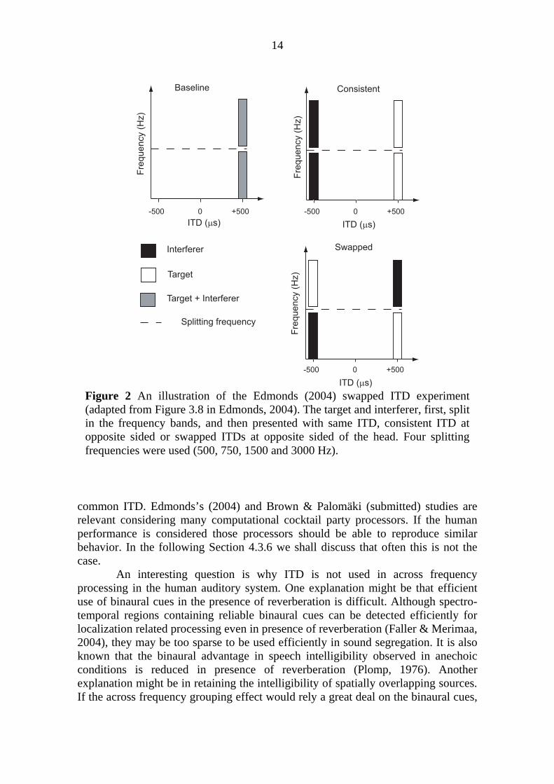
Edmonds (2004) extended the studies conducted with isolated vowels (e.g. Culling & Summerfield, 1995; Darwin & Hukin, 1997; Drennan et al., 2003) by an intelligibility test of real continuous speech via a speech reception threshold (SRT) measurement. Figure 2 depicts one of his experimental setups. Speech and interferer were first split into high and low frequency bands. Then the target and interferer were presented with three different ITD configurations: one, both in the right side ("baseline"), two, interferer on the left, target on the right ("consistent"), and three, low and high frequency parts of the interferer split in the left and right sides, respectively; low and high frequency parts of the target split on the right and left sides, respectively ("swapped"). Comparing the "baseline" to "consistent" and “swapped” conditions, he demonstrated that ITD separation of target and interferer improves speech intelligibility (due to binaural masking level difference, see Moore, 1989 for review). Moreover, he found that intelligibility did not differ between "consistent" and "swapped" cases, which suggests that common ITD does not mediate across frequency grouping. This is because the target was equally intelligible even though target frequency bands were divided to opposite ears (vice versa for the interferer). Only the (constant) amount of separation between target and interferer mattered. However, recent replication of Edmonds experiment (2004) by Brown & Palomäki (submitted) demonstrate that the intelligibility in the "consistent" case is slightly superior than in the "swapped" case. This advantage may be related to small benefit in the across frequency grouping mediated by the

14

-500 0 +500 -500 0 +500

ITD (μs) ITD (μs)

Fre

qu

en

cy (

Hz)

Fre

qu

en

cy (

Hz)

0 +500-500

ITD (μs)

Fre

qu

en

cy (

Hz)

Interferer

Target

Target + Interferer

Splitting frequency

Baseline Consistent

Swapped

Figure 2 An illustration of the Edmonds (2004) swapped ITD experiment (adapted from Figure 3.8 in Edmonds, 2004). The target and interferer, first, split in the frequency bands, and then presented with same ITD, consistent ITD at opposite sided or swapped ITDs at opposite sided of the head. Four splitting frequencies were used (500, 750, 1500 and 3000 Hz).

common ITD. Edmonds’s (2004) and Brown & Palomäki (submitted) studies are relevant considering many computational cocktail party processors. If the human performance is considered those processors should be able to reproduce similar behavior. In the following Section 4.3.6 we shall discuss that often this is not the case.

An interesting question is why ITD is not used in across frequency processing in the human auditory system. One explanation might be that efficient use of binaural cues in the presence of reverberation is difficult. Although spectro-temporal regions containing reliable binaural cues can be detected efficiently for localization related processing even in presence of reverberation (Faller & Merimaa, 2004), they may be too sparse to be used efficiently in sound segregation. It is also known that the binaural advantage in speech intelligibility observed in anechoic conditions is reduced in presence of reverberation (Plomp, 1976). Another explanation might be in retaining the intelligibility of spatially overlapping sources. If the across frequency grouping effect would rely a great deal on the binaural cues,

15

it is possible that they would override some important monaural cues (common f0, common onset, etc.). This in turn might lead to misjudgments about the source origin of spectro-temporal regions in cases where spatial location of sources overlap.

In summary, it has been noted that spatial separation of target and interfering signals improves in the segregation of the target out of a complex acoustic mixture. How this process is carried out in the human brain is not altogether clear. Currently, leading opinion is that ITDs (the main cue for localization) do not mediate grouping across frequency, but might be useful in grouping across time. Other cues, such as common fundamental frequency, might be more powerful in across frequency grouping. However, as controversial evidence exists (Drennan et al., 2003), the issue still essentially requires further clarifying studies. The explanation of why binaural cues are not used in across frequency grouping possibly originates from their compromised effectiveness in the presence of reverberation. Also, in order to avoid ambiguities in the case of spatially overlapping sources, it may be beneficial to emphasize monaural cues over binaural ones in the across frequency grouping.

2.4 Modulation frequencies in speech segregation In addition to location cues in the auditory signals, room reverberation also tends to smooth spectro-temporal structure of speech by filling the gaps between strong speech regions (see Figure 3 left panel). Human listeners appear to have remarkable tolerance to reverberation especially in one-talker situations. Nabelek and Robinson (1982) show that speech recognition accuracy for the anechoic case is 99.7% and degrades to 97,0%, 92.5% and 88.7% for reverberation times of 0.4 s, 0.8 s and 1.2 s, respectively. The effect of reverberation becomes more disrupting in the presence of multiple competing voices (Culling et al., 2003).

Tolerance of slowly varying interference such as stationary noise or reverberation has been explained by the capability of human hearing to focus on temporal modulation characteristics unique to speech, which are at their strongest at modulation frequencies roughly between 1 to 16 Hz (Houtgast & Steeneken, 1985; Drullman et al., 1994a, 1994b). The most important 3-4 Hz modulation frequency range reflects the syllable rate of speech originating from the articulatory movements (Houtgast & Steeneken, 1985), which in turn convey the linguistic message in speech. For example, modulations faster than those related to articulation, are those related to vocal fold vibration (e.g. fundamental frequency). The fundamental frequency itself does not carry articulatory information, but is rather a carrier signal, which can be used in varying intonation or expressing emotions. Modulations slower than those of articulation often originate from the environment: transmission line, reverberation, or an active noise source, such as traffic on busy roads. Similarly, slow modulations of speech spectra are important for speech intelligibility, as they carry information about formants, which are crucial in determining phoneme identities. Again, slow modulations like spectral tilts do not originate from articulation but are affected by, for example, transmission

16

(e.g. telephone line, reverberation). Fast spectral modulations again relate to the harmonic structure originating from vocal fold vibration periods.

In fact, the preservation of speech modulations in room reverberation can be characterized by measuring the modulation transfer function (MTF), which can be used for prediction of speech intelligibility in the corresponding reverberation conditions (Houtgast & Steeneken, 1985). From the MTF, it is possible to observe how important speech modulations (1 to 16 Hz) are preserved in reverberation; furthermore, MTFs can be used to estimate the equivalent signal-to-noise-ratio comparing reverberation to a wide band noise masker. Thus, the prediction power of the MTF in speech intelligibility clearly demonstrates the importance of preserving modulation frequencies characteristic to speech. The right panel of Figure 3 shows an example of the effect of reverberation on speech modulations comparing the modulation transfer for anechoic and 1.2 sec reverberation time conditions. The top right panel demonstrates that the magnitude of the higher modulation frequencies decreases more steeply for the reverberant than for the anechoic condition. The modulation transfer estimate for the utterance example shows that the attenuation of temporal modulation in the example reverberation conditions (reverberation time 1.2 s) corresponds roughly to the theoretical MTF obtained using the Houtgast & Steeneken (1985) method up to about 8 Hz. Modulations above 8 Hz for the example utterance are attenuated for both the anechoic an reverberant sample so much that the estimate no longer is reliable. The

Time (s)

Fre

quen

cy (

Hz)

0.4 0.8 1.2 1.6 2 2.4 2.8 3.2

379

1215

3202

Time (s)

Fre

quen

cy (

Hz)

0.4 0.8 1.2 1.6 2 2.4 2.8 3.2

379

1215

3202

100

101

−20

−15

−10

−5

0

Modulation freq. (Hz)

Fre

quen

cy (

Hz)

100

101

−10

−5

0

Modulation freq. (Hz)

Fre

quen

cy (

Hz)

Figure 3 Auditory spectrograms (left panels) for a male utterance "five seven four three two five one" in anechoic (top left) and reverberated (bottom left, reverberation time 1.2 s) conditions. Modulation spectra of these same samples (top right), where spectra of anechoic and reverberated utterances are shown with the solid and dashed lines, respectively. Description of the effect of reverberation (bottom right) in the modulation transfer characteristic of the same room. The solid graph is obtained by subtracting the modulation spectra of the anechoic sample from the reverberant sample. The dashed line shows a theoretical curve obtained from the modulation transfer function of Houtgast & Steeneken (1985). The straight line shows the effect of white noise in modulation transfer at zero dB SNR.

17

largest magnitude in modulation spectra of the example occurs at around 1.5 Hz, because this particular example is uttered in two parts that are separated by a long temporal gap. Other peaks seen between 2 and 4 Hz reflect the syllabic structure.

During the development of the channel vocoder in Bell Labs, Dudley (1939) gathered some of the earliest evidence regarding the importance of the slow modulations on speech intelligibility. The channel vocoder consists of a source signal and a filter model of the vocal tract estimated from a real speech signal. Either a periodic signal from a pulse generator ("buzz") or aperiodic noise signal ("hiss") were used to model voiced and unvoiced excitation, respectively. Even with slowly varying parameters of the vocal tract filter, they were able to produce highly intelligible speech. The vocal tract filter control parameters were low-pass filtered using a filter emphasizing mostly frequencies below 10 Hz (cut-off at 25 Hz).

Drullman et al. (1994a, 1994b) investigated effect of reducing slow or fast temporal modulations on speech intelligibility obtained by high or low-pass filtering the temporal envelope in frequency bands, respectively. Here, approximately the same modulation frequency range seems to account for speech intelligibility. Shifting the low-pass cut-off frequency of the envelope filter below 16 Hz results in reduced intelligibility, whereas shifting it upward does not result in any changes (Drullman et al., 1994a). Similarly, shifting high-pass cut-off frequency below 4 Hz does not result in loss of intelligibility (Drullman et al., 1994b).

Greenberg et al. (2003) underline the importance of the temporal properties of speech. They state that the ability to understand spoken language depends on the broad distribution (50-400 ms) of syllable duration, which corresponds to the 2.5-20 Hz modulation frequency range. Based on analysis of speech originating from American English telephone conversations, they show that unstressed syllables and stressed syllables are reflected to the upper (6-20 Hz) and the lower (<5 Hz) branches of the modulation spectrum, respectively. Segments are generally longest for stressed syllables and shortest for unstressed syllables. Singh & Theunissen (2003) extend the discussion beyond human language to other behaviorally relevant sounds. They state that most natural sounds are low-passed, and have most of their modulation energy at low spectral and temporal modulations. Further, animal and human vocalizations contain most of the spectral modulation power only in the low temporal modulation. This evidence leads the authors to postulate that the auditory system exploits these statistical properties of sound signals in order to achieve effective representation for behaviorally relevant sounds.

In summary, previous research has clearly demonstrated the importance of the modulation frequency range of about 0.5 to 16 Hz for speech intelligibility. This region is important, as it conveys information about the syllabic structure of speech due to articulatory movements. Studies of the modulation transfer function demonstrate that preservation of this modulation frequency range determines intelligibility when speech is contaminated by reverberation or stationary noise. The importance of modulation frequencies in speech segregation is highlighted in this thesis, showing an approach using modulation filtering in speech segregation from reverberation noise (P6).

18

3 Processing auditory space and speech in the brain In this section the brain processes underlying sound localization are addressed. Spatial processing along auditory pathways has traditionally been researched using animal models. The work on animal models reviewed here concentrates on finding cells or cell groups responsive to spatial stimuli through an invasive measurement from electrodes placed on neurons in the brain (Sect. 3.1, for reviews see: Casseday & Covey, 1987; Kuwada & Yin, 1987; Cohen & Knudsen, 1999). Using this method, information from cells or cell groups can be recorded for building models of neural computations related to spatial hearing and localization. Recently, non-invasive measurement techniques have allowed studies of the human brain. Although not as precise as in the cellular level, non-invasive methods allow the use of human subjects and thus investigations of higher level processes which might be unique to humans. Developments of these methods also allow rather accurate (~1 mm) spatial localization of the brain activity as well as good temporal accuracy. Sect. 3.2 addresses the application of these methodologies to research of spatial hearing in human subjects. Sect. 3.3 is devoted to studies on evoked response studies on the human speech processing, and spatial processing with speech signals.

3.1 Spatial auditory processing in animal models

Pathways. The central auditory pathways are divided into separate monaural and binaural pathways (for a review, see Casseday & Covey, 1987), the latter being particularly important for sound localization. The left-hand side of Figure 4 depicts the binaural pathway, and the right hand side shows its top-down connections to associative, motor and visual areas necessary to produce motor responses to spatial stimuli (for more details see Cohen & Knudsen, 1999). The origin of binaural pathways is the anteroventral cochlear nucleus (AVCN), from where it ascends to the superior olivary complex (SOC), then directly and indirectly (through the dorsal nucleus of lateral lemniscus) to the inferior colliculus (IC), to the auditory thalamus and then to the primary auditory cortex (AI). In mammals, the first site of binaural comparison is in the SOC, within which ITDs are coded in the medial superior olive (MSO) and ILDs in the lateral superior olive (LSO) (Cohen & Knudsen, 1999). Most of the cells in the MSO are sensitive to low frequencies, which is consistent with the dominance of ITD in the low frequency range. Similarly, cells in the LSO are sensitive at the high frequency range where ILD dominates. Lesions in this level cause localization defects bilaterally or in the auditory field ipsilateral to the brain side, whereas lesions in the ascending processing sites cause contralateral localization defects (Jenkins & Masterton, 1982). Thus, the authors conclude that the trapezoid body of superior olivary complex accomplishes the contralateralization of the auditory field.

The next major binaural computation stage is in the IC, where both ITD and ILD are processed (Kuwada & Yin, 1987; Cohen & Knudsen, 1999). In the

19

nontonotopic (neurons respond to wide range of frequencies) subdivision of the IC, the information about spatial cues is combined across frequencies (Cohen & Knudsen, 1999). This is regarded as a first step towards the formation of a spatial map. Based on evidence of many mammalian species, the tonotopic representation is transformed to spatiotopic in the external nucleus of the inferior colliculus ICX (Cohen & Knudsen, 1999). In the IC, the auditory pathway branches towards the primary auditory cortex through the medial geniculate body of the auditory thalamus, and also towards the superior colliculus (SC) through the ICX.

The SC contains a map for auditory space, which is used for orienting eyes and head (Cohen & Knudsen, 1999). As in the ICX, neurons in the SC are tuned broadly for frequency, but sharply for spatial location. A map for contralateral auditory regions exists in the each side of brain. Moreover, a map of visual space coexists in these same structures.

Although the medial geniculate body (MGB) in the auditory thalamus resides between the inferior colliculus and the auditory cortex along the binaural

Primary

auditory

cortex

Auditory

thalamus

Inferior

colliculus

MSO LSO, DNLL

Cochlear

nucleus

Associative

areasFEF

Superior

colliculusICX

Tegmental

pre-motor

nuclei

Binaural pathway

Figure 4 Pathway of auditory-space processing. Binaural auditory pathway shown on the left. Boxes show anatomical structures of the auditory pathway. Abbreviations: lateral and medial superior olives, LSO and MSO, respectively; dorsal nucleus of lateral lemniscus, DNLL; external nucleus of inferior colliculus ICX; frontal eye field, FEF (adapted from Cohen & Knudsen, 1999).

20

pathway, the processing of spatial information in the MGB has not been studied in detail (Casseday & Covey, 1987; Cohen & Knudsen, 1999).

The primary auditory cortex retains a tonotopic coding, where neurons are organized in the iso-frequency layers with frequency increasing from caudal (toward head) to rostal (toward rear) (Casseday & Covey, 1987). It has been shown that binaural clusters of neurons with similar sensitivities are orthogonal to the iso-frequency layers (Middlebrooks & Zook, 1983; Casseday & Covey, 1987). However, this representation is not topographically organized, as neighboring clusters are not interrelated in terms of their directional sensitivity (Cohen & Knudsen, 1999). Using extra cellular recordings Brugge & Reale (1996) measured spatial receptive fields of neurons in the auditory cortex of a cat. About 69% of studied neurons had receptive field of frontal, contra- or ipsilateral quadrant of the auditory space, with the largest proportion of neurons being responsive to sound sources in the contralateral quadrant. Thus, the authors suggest that these spatial receptive field properties of the neurons could aid in signaling the sound source direction.

Lesion studies in macaque monkeys suggest that the primary auditory cortex is of importance in the auditory spatial processing. Hefner (1997) demonstrated that bilateral ablation of auditory cortex caused sensory and perceptual defects in localization. The sensory defect was demonstrated as follows: After ablation monkeys were able only to discriminate between the left and right hemifield directions, whereas the discrimination for sound sources within the left or right hemifields were almost totally destroyed. The perceptual defect was demonstrated by the observation that monkeys do not associate a sound with a location in space. This was indicated by the inability of thirsty monkeys to approach the location of a water reward as cued by spatial auditory stimuli. Also, lesions in the frontal eye field have demonstrated a substantial decrease in monkey’s performance in discrimination of sound location (Cohen & Knudsen, 1999). Computation. Considering the computational processes for spatial localization, Jeffress (1948) proposed a hypothesis about a specific coincidence mechanism for detection of interaural delays (see Figure 5). This would consist of neuronal delays and coincidence counters between delayed signals originating from each ear. The coincidence counter peaks when left and right ear signals coincided at the delay line position, which corresponds to interaural delay of the acoustic waveform. Jeffress's theory has inspired a large body of physiological research on the existence of the coincidence mechanism, as well as attempts to build plausible computational models (see Sect. 4.3.3). Finding that the MSO receives inputs from cochlear nuclei of both sides showed that the MSO has binaural function, and gave a clue that Jeffress’s theory might be physiologically plausible (Stotler, 1953; Casseday & Covey, 1987). After this, more evidence has been gathered about the existence of coincidence detector neurons in the medial superior olive, dorsal nucleus lateral lemniscus and inferior colliculus, or their avian homologues as indicated in extensive studies of barn owl (Takashi & Konishi, 1986; for review, see Kuwada & Yin, 1987).

21

Only recently was serious criticism about the existence of a coincidence counter mechanism proposed by McAlpine et al. (2001). In a single cell recording of a gerbil's inferior colliculus, they found that neurons tuned to low best frequencies (BF) reach peak activity well beyond the plausible range of contralateral ITD with respect to their head size. First, they observed that the ITD at which a neuron peaked decreased in a near-linear fashion on the logarithmic best frequency of the neuron. Thus, the interaural phase difference at which neurons peaked was nearly constant across frequency. Next, they found that increasing the contralateral ITD resulted in increments of neuronal firing rate up to the peak ITD. However, the increases in the sound pressure level (SPL) elevate the activity of these neurons as well. Therefore, in order to take into account the increase in SPL, the authors suggest comparison of activity in each hemisphere. Observations by McAlpine et al. (2001) are, in fact, somewhat consistent with observations in the human auditory cortex as indexed by N1m amplitude (McEvoy et al., 1993; P1; P2; P4). Each hemisphere shows tuning to sound source direction so that the responses increase as sound source location is varied from ipsi- to contralateral locations. In summary, animal studies have been useful in both localizing binaural processing centers of the brain, as well as in clarifying computational mechanisms of processing of spatial cues. The main centers for binaural interaction at the brain stem level are the superior olivary complex and the inferior colliculus, in which neurons sensitive to ITD and ILD have been registered. The auditory cortex is also important for spatial localization. Cells in the auditory cortex have spatial receptive fields, and ablations of the auditory cortex result in severe defects in space processing. The specific coincidence mechanism for computation ITD has been already proposed by Jeffress (1948), and since then has been widely accepted. In the publication presenting a binaural processor (P5) in this thesis, a modified version of Jeffress’s (1948) model is used. However, recent criticism by McAlpine et al. (2001) indicates that Jeffress’s theory may need to be revised. Interestingly, similar

Left Right Figure 5 Schematic diagram of a neural coincidence detector adapted from Jeffress (1948). The coincidence detectors receive their input from nerve fibers carrying signals from the left and right ears. The propagation delay is proportional to the length of nerve fibers.

22

signalings of sound source directions are observed in the McAlpine et al. (2001) study of the gerbil IC and in the level of the auditory cortex in the measurements conducted in this thesis (P1; P2; P4; see Sect. 3.2).

3.2 Spatial auditory processing in humans Modern non-invasive brain measurement techniques have allowed research on sound localization in the human brain (see Figure 6 for an illustration of auditory pathways in the human brain). The neuronal currents in the brain cause deviations in the scalp recorded potential (electroencephalography, EEG) and in the magnetic field (magnetoencephalography, MEG) recorded outside the head (Näätänen & Picton, 1987; Hari, 1990; Hämäläinen et al., 1993; Eggermont & Ponton, 2002). Using these techniques, the brain's neuronal responses to sensory stimulation can be measured with good temporal accuracy in terms of the event-related potential (ERP) and magnetic field (ERF). From the ERP and ERF responses auditory cortical activity is often be indexed by their largest deviation the N1 (Davis, 1939; Näätänen

Auditory

cortex

Inferior

colliculus

Medial

geniculate

Cochlear

nucleus

Superior

olive

Figure 6 Main processing sites along the auditory pathway from the cochlea to the auditory cortex (adapted from page 201 in Kalat, 1992). Both the left and right hemisphere contain the same structures, which here are named only in the left hemisphere.

23

& Picton, 1987) or mismatch negativity (MMN) (Näätänen et al., 1978, May et al., 1999; May & Tiitinen, 2004; Jääskeläinen et al., 2004, Näätänen et al., 2005). The latencies of N1 and MMN are about 100 ms and 150-200 ms, respectively. For a more detailed explanation of these responses, see Sect. 4.2.2 More recently, brain imaging techniques such as functional magnetic resonance imaging (fMRI) and positron emission tomography (PET) used in measuring brain's hemodynamics have become prevalent due to their good spatial accuracy.

Studies in animal models indicate that contralateralization in the binaural pathway occurs between the superior olivary complex and inferior colliculus (Jenkins & Masterton 1982; Casseday & Covey, 1987; see Sect. 3.1). Consistent with that, ERP and ERF studies in humans have given supporting evidence of contralateral processing of the auditory stimuli in the auditory cortex. Cortices in both hemispheres respond more vigorously when the contralateral ear is stimulated monaurally (Wolpaw & Penry, 1977; Reite et al., 1981; Pantev et al., 1986; Woldorff et al., 1999) or if the sound is presented from the contralateral hemifield using virtual sound techniques (P1; P2; P4; Fujiki et al., 2002). When sound was lateralized via ITD, McEvoy et al. (1993) found similarly contralaterally more prominent responses, whereas Woldorff et al. (1999) found no difference in activation between contra- and ipsilateral stimuli. This may, however, be related to differences in stimulation methods (click train (McEvoy et al., 1993) vs. frequency sweep (Woldorff et al., 1999)). Supplementary observations were made in hemodynamic studies by Alho et al. (1999) and Petkov et al. (2004). By applying PET, Alho et al. (1999) found that directing attention to the left or right monaural tone stimuli induce contralaterally predominant activation in the right or left auditory cortices, respectively. Furthermore, by applying fMRI, Petkov et al. (2004) were able to connect hemodynamic measures to brain structural images. Larger activations were observed for monaural stimulations of the contra- than for the ipsilateral ear at around Hecsel’s gyri for both the left and right hemispheres.

Several researchers report ERP or ERF responses which vary consistently as a function of stimulus location (e.g. Paavilainen et al., 1989; McEvoy et al., 1993; P1; P2; P4). Paavilainen et al. (1989) found that the MMN-component of ERP increased along increasing lateral distance between standard and deviant stimuli. Their stimuli consisted of low and high frequency tones (600 and 3000 Hz, respectively) lateralized using ITD and ILD, respectively. MMN was also observed in free-field condition, but no consistent effect of stimulus deviance was found in this case. Investigating N1m (ERF component) in the right hemisphere McEvoy et al. (1993) found that the N1m response increased along the increasing contralateral ITD. Applying virtual spatial stimuli, Palomäki et al. (P1, P2, P4) found that N1m in both the left and right hemispheres increased when the source location was varied from ipsi- to contralateral horizontal directions (see Figure 7).

Zatorre & Penhune (2001) point out that, unlike in animal models, the right hemisphere of the human brain appears to be more dominant in auditory spatial processing. Indeed, the importance of the right hemisphere in auditory spatial processing is highlighted in many brain measurement studies (Bushara et al., 1999; Kaiser et al., 2000a; P1; P2; P4; Zatorre et al., 2002) in studies with patients suffering from auditory neglect (Deouell et al., 2000; Deouell & Soroker, 2000;

24

Zatorre & Penhune 2001) and behavioral studies (Burke et al., 1994; Butler et al., 1994). In our two studies (P1; P2), we found that the amplitude of N1m in the right hemisphere is larger when compared to that of the left. Moreover, response dynamics for contra- vs. ipsilateral stimulation were larger in the right hemisphere. Initially, Palomäki et al. (P1) showed these results to account for broadband noise stimuli, and they were further extended to account for speech (vowel stimuli) Palomäki et al. (P2). However, differences in hemispheric dominances at the individual level have also been reported (Fujiki et al., 2002), although in the same study the authors point out that spectral cues are processed predominantly in the right hemisphere. Kaiser et al. (2000a) measured MMN and gamma band activity for ITD-lateralized speech. MMN latencies were faster in the right hemisphere and the gamma band activity (around 53 Hz) increased in the right hemispheric posterior pariotemporal region. Both of these observations suggest the right hemispheric dominance in processing of lateralized stimuli. Applying the fMRI measurement on hemodynamics, Petkov et al. (2004) suggested that stimulus dependent activations, such as left-right stimulations, elicit more prominent activation in the right hemisphere, whereas attention dependent activations are stronger in the left hemisphere.

In human patients, it has been observed that lesions in the right hemisphere may lead patients to neglect auditory stimuli in the left hemifield, whereas no similar neglect is observed after left hemispheric damage (Pinek et al., 1989; Deouell & Soroker, 2000). Deouell & Soroker (2000) suggested that this is a defect in spatial processing, which highlights the crucial role of the right hemisphere in spatial processing. The lesions in the Deouell & Soroker (2000) study were located all in the right hemisphere. Although the exact locations varied among the patients, they all exhibited auditory neglect in the left hemifield. However, in contradiction to the right hemispheric processing hypothesis, Pinek et al. (1989) reported that left hemispheric patients (lesions mainly in left parietal areas) exhibited more severe

-

-

-

40

80

120

40

80

120

Left hemisphere Right hemisphere

0 45 90 135 180 -135 -90 -45

Angle (deg)N

1m

am

plit

ude (

fT/c

m)

Angle (deg)

0 45 90 135 180 -135 -90 -45

Figure 7 This example is taken from the P4. The left panel shows the array of stimulus directions used in the study. Middle and right panels show N1m responses over the left and right hemisphere, respectively. In both hemispheres, ascending organization of the amplitude is noticed as the sound source location is varied from ipsi- to contralateral. The responses are larger in the right hemisphere.

25

problems in localization than right hemispheric patients (lesions mainly in right parietal areas). Further, in the behavioral measurements of the localization accuracy, Burke et al. (1994) found that free-field localization is more accurate in the left hemifield. Based on the contralateral processing principle, they interpret this as right hemispheric dominance. A related observation was made by Butler (1994) in a monaural localization task, where subjects located sounds in the median plane more accurately using the left ear, which shows right hemisphere advantage.

Two ERP studies have compared the processing of ITD and ILD cues, suggesting that they are processed by different systems (Schröger, 1996; Ungan et al., 2001). Ungan et al. (2001) found that ERP responses to ITD- and ILD-stimuli had significantly different scalp topographies. Investigating the MMN, Schröger et al. (1996) found that combined ITD and ILD deviants elicited a larger amplitude MMN than deviants, which contained either ITD or ILD cues alone. The summed amplitude of ITD and ILD alone deviants matched the amplitude of ITD and ILD in combination, suggesting that ITD and ILD are combined in a near-linear process. Similar results were obtained by Palomäki et al. (P4), where ipsi- vs. contralateral response dynamics of the right hemispheric N1m were twice as large for the combined ITD and ILD stimuli as for the ITD or ILD alone stimuli. In the same study, dynamics increased further when subjects’ individual virtual spatial stimuli were used. Compared to ITD- and ILD-based lateralized stimuli of Schröger (1996) and Ungan et al. (2001), the individual virtual spatial stimuli by Palomäki et al. (P4) added the spectral cues to stimuli, and made stimuli to appear outside of the head.

By exploiting individual HRTF-based spatial stimuli, Fujiki et al. (2002) observed that azimuthal deviants elicit MMN earlier than elevation deviants. From this observation, they concluded that the auditory cortex processes binaural cues earlier (100-150 ms) than spectral cues to location (200-250 ms). They also suggested that spectral cues were processed predominantly in the right hemisphere. Related conclusions were made by Kaiser et al. (2000b) observing that ITDs were processed earlier (110-140 ms) than spectral variation in the stimuli (around 180 ms). Palomäki et al. (P4) found a location shift between N1m for realistic virtual spatial stimuli incorporating prominent spatial cues (ITD and ILD in combination with the spectral cues) vs. impoverished spatial cues (ITD or ILD alone or in combination). Thus, adding spectral cues to the stimuli caused anterior location shift of equivalent current dipole (ECD) already at the time span of N1 (around 100 ms).

Behavioral studies have originally found the existence of a spatial gradient in attention, which means that attention can be focused most effectively only on a sector of space at a time instant. Teder & Hillyard (1998) and Teder et al. (1999) found a neuroelectric correlate in ERPs for a behaviorally observed attentional gradient. In ERPs, the gradient is noticed in increased responses for stimuli nearby to the focus of spatial attention. ERP increments were observed at 80-200 ms (processing negativity) and at around 250 ms latencies, the former involving a broader spatial gradient sector than the latter. Considering those two time intervals, the authors suggest that spatial auditory attention might be focused in two stages: first, involving broader focus; second, being more narrowly focused. Their ERP attentional gradients were strongly correlated with behaviorally measured detection

26

rate (Teder & Hillyard, 1998; Teder et al., 1999). Applying more spatially precise MEG measurements, Rif et al. (1991) studied attentional effects for monaural tonal stimuli. In their second experiment, subjects were presented with equiprobable 1 and 3 kHz tones to each ear. The duration of both 1 and 3 kHz stimuli was varied, where standard (occurring 90% of time) and deviant (occurring 10 % of time) durations were 50 and 100 ms, respectively. Subjects were instructed to count deviants in one ear at time (relevant channel) and ignore all stimuli in the other ear (irrelevant channel). When subtracting responses of irrelevant channel from those of relevant, they observed an attentional effect called magnetic difference, Md, which started at 30-40 ms and increased the amplitude of N1m. Considering this thesis, the investigation of the attentional effects using MEG and realistic spatial stimuli is clearly an interesting future direction.

Studies using hemodynamic measures (Bushara et al., 1999; Griffiths & Green, 1999; Martinkauppi et al., 2001; Zatorre et al., 2002) have found areas beyond the auditory cortex that are activated by spatial sound stimulation. In these studies, it is typical that many subsequent stimuli with changes in their spatial properties are presented to the subject over longer durations of time, after which the brain is scanned for increments in the blood flow. Applying this method, centers that are active due to the spatial content of stimuli can be found, but differences in processing of individual directions cannot be observed. Bushara et al. (1999) found that during visual and auditory spatial stimulation, blood flow increased in the superior parietal and prefrontal cortices in areas that were specific to the modality (visual or auditory). Further, Zatorre et al. (2002) found that spatial stimuli presented simultaneously from different locations elicit activity in the posterior auditory cortex. Moreover, during the spatial localization task they found that the inferior parietal cortex is activated and that the strength of the activation correlates positively with behavioral localization error of the individual subjects. This indicates that subjects capable of localizing spatial stimuli accurately recruit less processing power in the parietal area. Complementary observations were made in the temporal lobe by Palomäki et al. (P4). They found that right hemispheric organization of the activation strength as indicated by N1m amplitude measured in the passive listening condition correlates with subjects’ localization accuracy. Thus, ascending ipsi- to contralateral order of the response strength predicted the subjects’ localization ability.

Alain et al. (2001) investigated “what” and “where” aspects of processing of auditory stimuli through pitch (what) and location (where) identification, and found that these tasks generated differential activation in the brain. Relative to the pitch task, the localization task generated more activity in the posterior temporal cortex, the parietal cortex, and the superior frontal sulcus of both the hemispheres. The pitch task generated more activity in both the auditory cortices and the inferior frontal gyrus. Task related differences were also found in ERP responses 300 ms after stimulation in anterior and posterior brain regions. When comparing hemodynamics in a localization vs. recognition task, Maeder et al. (2001) found that activation of the fronto-parietal convexity differed in the two tasks. Relative to recognition, the localization task generated more activity in both hemispheres in the lower part of the inferior parietal lobule and the posterior parts of the middle and

27

inferior frontal gyri. The recognition task generated more activation bilaterally in the middle temporal gyrus and the precuneus, and in the left hemisphere in the posterior part of the inferior frontal gyrus. In summary, studies in humans have mostly considered sound localization on the level of the auditory or parietal cortex. Based on these studies, auditory cortices in both hemispheres seem to be sensitive to sound direction. Responses increase when sound location is varied from ipsi- to contralateral (processing latency around 100 ms). Some authors have suggested that spectral cues are processed later, around 180 ms or 200-250 ms. Most studies report right hemispheric dominance in the processing of spatial sound, which starts already from the level of the auditory cortex. Perhaps the most common finding beyond the temporal lobe is the recruitment of the parietal lobe in auditory spatial processing. Both studies in the auditory cortex (temporal lobe) and parietal lobe have found correlates of activation with localization accuracy. In the right temporal lobe, systematic ipsi- vs. contralateral angular organization of the activation has been able to predict subjects’ localization accuracy. In the right parietal lobe, the activation is stronger for those subjects with weak localization performance, indicating that a good localizer recruits less processing power.

3.3 Processing of speech and speech presented spatially Considering the auditory processing in the human brain, speech is of utmost importance. The information relevant to the recognition of speech is carried in the spectro-temporal structure of the speech signal. Spatial localization becomes important, for instance, in directing attention towards an interesting speaker in a cocktail party (see Sect. 2.3). Furthermore, it has been observed that spatial separation between target and interferer improves the intelligibility of the target (see Sect. 2.3).

With the introduction of non-invasive brain measurement technologies, the investigation of brain processes underlying speech perception has recently received much attention. However, studies specifically concentrating on speech presented spatially remain rather scarce (Kaiser et al., 2000a; P2). On the other hand, a great deal of brain research on spatial hearing has used non-speech stimuli (e.g. Kaiser et al., 2000b; P1; P4; Fujiki et al., 2002), possibly in order to avoid activating processes specific to speech. In this section we will be restricted to studies concentrating on the auditory N1m-response, which is the most relevant background of all the MEG studies in this thesis. There exists also a large body of literature on speech processing with MMN response (e.g. Näätänen et al., 1997; Alho et al., 1998; Tervaniemi et al., 1999; Rinne et al., 1999; see Näätänen, 2001 for review).

Studies on N1 response have been able to register latency (Diesch et al., 1996; Poeppel et al., 1997; Obleser et al., 2003) and source location (Diesch et al., 1996; Diesch & Luce, 2000; Mäkelä et al., 2003) variation between responses to different vowel identities. This suggests that brain processes as early as those underlying N1 might already determine the vowel identity. Through applying vowels with large contrasts between first and second formant (F1 and F2, respectively), Mäkelä et al. (2003) found that the loci of N1m response in the left

28

hemisphere varied as a function of the distance of F1 and F2, whereas right hemisphere source loci were not sensitive to vowel identity. These results indicating sensitivity of N1m of the left hemisphere are also are supported by studies applying MMN (Näätänen et al., 1997; Alho et al., 1998; Rinne et al., 1999), where left hemispheric speech specificity is observed also. Generally, the issue that these observations are specific for the left hemisphere is in line with the theories that the left hemisphere is specialized in the processing of speech and language (for review see Gazzaniga et al., 1998).

However, it is difficult to see whether these response differences between vowel identities are genuine effects of changing vowel categories or whether they are just due to spectral differences. A study on the auditory MMN by Näätänen et al. (1997) provides an interesting viewpoint on this by presenting vowel stimuli for subjects of two different languages (Finnish and Estonian). They found that for native Finnish speakers, the Finnish language vowel deviants elicit larger MMN than the Estonian language vowel deviants, and vice versa for native Estonian speakers. Furthermore, enhancement of MMN in native Finnish speakers occurred for the Finnish language vowel deviant in which F1 and F2 were closer to those of standard stimuli than were the F1 and F2 of Estonian vowel stimuli when compared to the same standard. Thus, responses were enhanced more to the native language vowel deviant, even though its acoustic deviance was smaller when compared to the standard. Therefore, it was concluded that acoustic differences in the stimuli cannot alone explain these response differences.

However, when presented spatially, speech stimuli seem to elicit a larger activation in the right hemisphere (Kaiser et al., 2000a; P2). As discussed in Sect. 3.2, a general observation is that the right hemisphere is specialized for processing of spatial stimuli. Interestingly, even though the spatially presented stimuli contain speech material, the responses, as well as response dynamics, are larger in the right hemisphere. Most of the N1 studies on diotically presented speech do not report significant differences between left and right hemispheric amplitude (Eulitz et al., 1995; Diesch et al., 1996; Alku et al, 2001), at least as long as attention is not engaged to the stimuli (Poeppel et al., 1996).

Another line of research in studies of brain processing of speech has been to contrast processing of speech stimuli with non-speech stimuli, like sinusoids (e.g. Tiitinen et al., 1999), random noise (P2) or random noise excited vowels (P3). Speech signals elicit markedly larger amplitude than random noise signals even if they are presented with equal energy i.e. near equal loudness (P3; P2). In their study, Alku et al. (P3, see also Alku et al., 1999) used a vocal tract filter estimated from a real vowel signal. They produced vowels by two types of excitation: (periodic) glottal pulse, and (aperiodic) random noise. The vocal tract filter was held constant for each vowel identity. Authors observed a marked decrement in the N1m amplitude when real glottal excitation was replaced by a random noise signal. Thus, the presence or absence of periodic structure has a strong influence on the N1m amplitude. However, verification of whether this N1m amplitude difference originates from the periodic aperiodic difference would also require tests with non-speech periodic stimuli such as square or triangular waves as opposed to random noise of a similar spectral shape.

29

In a PET study of hemodynamics, Alho et al. (2003) found that attention to speech stimuli presented either auditively to the left or right ear, or visually as text enhanced the activation of the superior temporal cortex in the language dominant left hemisphere. Furthermore, the activity in the middle temporal cortex of the right hemisphere was enhanced. The latter result was interpreted as enhanced processing of prosodic features. Increased activation was also observed in the right parietal cortex area, which is important in directing spatial attention (e.g. Zatorre et al., 2002).

In summary, the processing of spatial speech stimuli still remains poorly understood, and requires further investigation. Studies regarding the processing of vowel identity suggest that it might be presented already in the latency span of N1 in the left hemisphere, indicating left hemispheric specialization. It is difficult to distinguish whether differences observed in the brain responses originated from genuine phoneme category discrimination. However, a study by Näätänen et al. (1997) show observations where differences in brain responses cannot be explained by the acoustical differences between stimuli, because the effects for the same stimulus conditions vary based on native language of the subjects. When speech is presented spatially, the right hemispheric responses are more prominent. An interesting issue to be addressed in the future is the role of attention in processing of spatially presented speech.

30

4 Applied research methods in brain measurements and auditory modeling

4.1 Technologies of 3D audio in brain imaging As reviewed in Sect. 2.1, spatial perception is mediated by the localization

cues (ITD, ILD and spectral cues) present in the signals received at both ears. Each direction has its own combination of these cues incorporating necessary information for localization. The question arises whether it is possible to artificially produce accurate spatial perception and mediate it through headphone listening. Considering brain imaging, this is a very interesting question. For fMRI or MEG, headphone audio is practically the only possibility for auditory stimulation. MEG is designed to measure weak magnetic fields generated by the brain’s neuronal activity, and therefore interference from any electrical device placed in the vicinity of the measurement coils will be harmful. This is problematic for auditory stimulation, as it excludes the use of conventional loudspeakers or headphones, or any electroacoustic transducer in the vicinity of the device. Therefore, a conventional dynamic loudspeaker (including ferromagnetic parts) needs be placed outside the magnetically shielded room, and sound is led to the listener’s ears through plastic tubes (the audio system used in the thesis is described in the Appendix in Sect. 8.1).

Due to problems in reproducing the spatial perception in headphone listening, ITD- and ILD- based stimuli have been used in previous MEG studies of spatial hearing. Using ITD or ILD stimuli location can be varied only laterally inside the head. Only when spectral cues are introduced will the stimuli appear in external locations; then they can be naturally perceived as originating from different directions. Due to recent advances in 3D audio technology, realistic spatial presentation of sound has become possible. In principle, it is possible to create a realistic spatial sound environment if the signals presented to the listener’s ear canals correspond exactly to those occurring during the desired spatial scenario. By placing miniature microphones in the listener’s ears, it is possible to binaurally record signals that incorporate the subject’s individual localization cues for any spatial scenario occurring during the recording (e.g. Plenge et al., 1974; Searle et al., 1975). This technique allows, for example, authentic spatial reproductions of concert hall recordings (page 358 in Blauert, 1997). Another possibility is to record the impulse response for the desired spatial configuration using microphones placed in the subject’s ears. These are called head-related impulse responses (HRIR), or perhaps more commonly, according to their frequency domain equivalent, head-related transfer functions (HRTFs) (Wightman & Kistler, 1989; Chapter 5 in Blauert 1997). HRIRs can be used for spatialization of an arbitrary sound signal via convolution, when sound is presented directly to subject's ears through headphones. HRIRs can also be used with stereo loudspeaker configuration, but in this case, the crosstalk totally absent in headphone listening has to handled. Techniques for 3D-audio are covered more comprehensively in review books (Begault, 1994; Chapter 5

31

in Blauert, 1997), and are also addressed in recent PhD theses from Helsinki University of Technology (Huopaniemi, 1999; Riederer, in prep).

The next question is whether, in practice, methods of 3D audio will allow perceptually accurate replication of this complex acoustic scenario. Wightman & Kistler (1989) investigated localization accuracy using individually recorded HRTFs in comparison with localization in free-field and found a somewhat close correspondence between them. The principal difference between free-field and HRTF stimulation was in the increase in number of front-back confusions, which was twice as large for HRTFs (10%) compared to free-field (5.6%) listening.

Recording HRTFs for each individual is a task requiring some rather special skills and equipment for acoustic measurements. Therefore, there is a need to find non-individualized HRTFs which are general enough to allow spatial presentation to any listener. Wenzel et al. (1993) have addressed this issue. Their general finding was that although the localization of sound in the azimuth was largely preserved, the accuracy in localization in the elevation (within cones of confusion) was diminished. In comparison between non-individualized HRTF and free-field stimuli, they observed 31% and 19% of front-back, 18% and 6% of up-down confusions, respectively. Considering the non-individualized HRTFs, the most frequently occurring confusion was front-to-back confusion (15%). Taking these findings together, they concluded that although ITD and ILD cues are robust even across individuals, the spectral cues due to the filtering effect of pinna head and body include subtle individual variations that are not well preserved across individuals. For the explanation of why front-to-back confusions occur more frequently than back-to-front, they suggested that the perceptual system would be more likely to spot ambiguous cases at the rear if the source of sound is not visible.

In summary, the recent advances in 3D audio technology have allowed the realistic reproduction of auditory space even in headphone listening. This is made possible either by binaural recordings or head-related transfer functions. In brain measurements, 3D audio technology has allowed the reproduction of auditory space in MEG and fMRI measurements where headphone stimulation is required. In this thesis, realistic spatial stimuli were produced using 3D audio technologies, and applied for the first time (P1) in MEG measurement.

4.2 Measuring auditory cortical responses using magnetoencephalography

4.2.1 Magnetoencephalography (MEG) All the brain measurements in this thesis have been conducted using the magnetoencephalography (MEG) measurement method (for MEG reviews see: Hari, 1990 Hämäläinen et al., 1993). Using MEG, weak magnetic fields generated by the neuronal currents in the brain can be measured outside the human skull. Neuromagnetic signals typically lie in range 50-500 fT (Hämäläinen et al., 1993). To give some perspective, the earth's geomagnetic field is from 108 to 109 times larger compared to fields generated by brain activity. Measurement of these signals is, indeed, technologically very demanding both in terms of sensitivity for the weak

32

magnetic fields and shielding of the outside electromagnetic interference. The introduction of the superconducting quantum interference device (SQUID; Zimmerman et al., 1970) made the development of MEG possible. The first SQUID measurement of the brain's magnetic field was performed by Cohen (1972) at the Massachusetts Institute of Technology.

The magnetic field observed outside the skull is produced entirely by tangential currents (spherical conductor). Radial currents do not result in a magnetic field outside the skull. Furthermore, the contributions of the sources deep inside the brain are weak in the MEG signals (Hari, 1990; Hämäläinen et al., 1993), as the magnetic field towards the center of the sphere attenuates rapidly, and is in fact zero at the origin. In contrast, the electric field component for both deep sources and radial currents produce stronger observable signals outside the skull. Thus, EEG captures all primary current components, but is more sensitive to the inhomogeneity of the human head as a conductor.

The strongest magnetic field component is produced by neuronal currents in the cortical fissures (Hämäläinen et al., 1993). The surface of the cortex is covered by layers of pyramidal cells with long axons (or dendrites) whose orientations are perpendicular to the cortex surface. Therefore, the currents in the pyramidal cells in the cortical fissures are tangential to the sphere conductor model and thus produce observable MEG signals. In the pyramidal cells, the postsynaptic potential (PSP) rather than action potential is the main cause of the MEG signal. From a distance, PSP resembles a current dipole oriented along the dendrite. The field of the dipole source attenuates according to 1/r2 law. The duration of a PSPs is typically tens of milliseconds, and therefore the total field component grows due to temporal integration for cell groups acting concurrently. In contrast, action potential, although producing larger magnitude currents, does not contribute strongly to the MEG signal. The reason for this is twofold: Firstly, the field produced by action potential attenuates faster along increasing distance than field caused by PSP. The field of action potential resembles a quadrupole (two oppositely oriented current dipoles) which attenuates by the 1/r3 law. Secondly, action potentials are very short – only around 1 ms in duration – and therefore do not integrate temporally as well as more long lasting PSPs.

4.2.2 Event-related potential (ERP) and magnetic field (ERF) Event-related potential (ERP) and magnetic field (ERF) are obtained by averaging EEG and MEG signal time locked to the stimulation. Typically, about a million synapses are simultaneously active during an evoked response (page 424 in Hämäläinen et al. 1993). In the averaging, it is assumed that brain activity not related to the event of interest is independent, and thus will be removed in the averaging process. Subsequent deviations in this response are related to neuronal activity in the brain areas activated in succession. The earliest components of the ERP response originate from sub-cortical sources. A recent study by Lütkenhöner et al. (2003) shows that the auditory cortex is already activated after about 20 ms latency. The electromagnetic fields measurable by EEG or MEG do not themselves contain structural information of the brain; thus, they cannot directly be used to relate the response locations to the brain structures. Therefore, tomography-based

33

methods have to be used for structural imaging, in which the source loci of MEG data can be substituted (e.g. Reite et al., 1994; McEvoy et al., 1997; Ohtomo et al., 1998). Recent developments have made it possible to connect functional MRI images to MEG evoked potentials, and thus to connect the hemodynamics to evoked responses (Liu et al., 1998). The particular interest of this thesis is the N1 (or N100) response and its magnetic component N1m occurring at about 100 ms after sound onset (Davis, 1939; Näätänen & Picton, 1987; see Figure 8 for an N1m response). For a comparison of N1 and N1m see e.g. Hari et al. (1982). Sustained stimuli are known to elicit N1 only at their onset. Prolongation of stimuli only up to 30-50 ms results in increases in the N1 amplitude. From this, it can be concluded that the N1 response is generated by cerebral processes which respond specifically to stimulus onsets (page 387 in Näätänen & Picton, 1987; see also Mäkinen et al., 2004 for recent data). In their comprehensive review of N1, Näätänen & Picton (1987)

−100 0 100 200 300−40

−20

0

20

40

60

Time (ms)

Am

plitu

de (

fT/c

m)

−100 0 100 200 300−40

−20

0

20

40

60

Time (ms)

Am

plitu

de (

fT/c

m)

-100 0 100 200 300

-20

0

20

40

60

Time (ms)

Am

pl. (

fT/c

m)

T=127.7 ms,Q=18.8 nAm

Figure 8 Illustrations of ERF response for auditory broadband stimuli. (Top) An ERF response at the MEG channel depicting maximal N1m over the right hemisphere of a single representative subject. The right and left panels show ERFs without filtering and filtered with a typical band-pass filter (2-30 Hz) setting, respectively. N1m is recognized as the strongest deflection from the zero line. (Bottom) The left panel shows a grand averaged (10 subjects) ERF response over the strongest right hemispheric channel for broadband stimuli originating from the left of the subjects. The right panel shows the corresponding dipolar field pattern.

34

describe six different temporally overlapping cortical processes (components) during the N1 response, from which they consider three as “true” N1 components controllable by stimulus parameters. Component one, located in the superior temporal plane, has tangential orientation and therefore is reflected in the magnetic recordings. Component two (T-complex by Wolpaw & Penry, 1975) is biphasic: positive wave at latency about 100 ms and negative wave at about 150 ms. It is thought to originate from the superior temporal gyrus (page 411 in Näätänen & Picton, 1987), and its orientation is predominantly radial. Component three is vertex negativity at about 100 ms, and may be generated by frontal and pre-motor structures. They propose that component four is a mismatch negativity (MMN), which is generated by an automatic change detection mechanism activated only if a change in the stimuli occurs (Näätänen et al. 1978; see Näätänen 1995, and Näätänen et al., 2005 for more recent reviews). MMN has been detected for rarely occurring deviants in a chain of frequently occurring standard stimuli. This was questioned by May et al. (1999), May & Tiitinen (2004) and Jääskeläinen et al. (2004), who argue that the appearance of the MMN is more likely related to neural habituation and adaptation, and does originate from the same processes as N1 response. However, in their more recent response to this debate, Näätänen et al. (2005) suggest, that there are some weaknesses in this habituation/adaptation hypothesis. Components five and six of N1 (Näätänen et al., 1987) originate from other specific processes related to processing negativity, i.e., an amplitude increment observed when directing attention to the stimuli. Several studies have been devoted to localizing the MEG component of N1 based on substituting ECDs to the MR images. Applying this approach, Reite et al. (1994) localized N1m source loci in auditory konio cortex in, or adjacent to, Heschl's gyri. By applying multiple measurements in "high precision" study of a single subject, Lütkenhöner & Steinsträter (1998) found the locus of the N1m peak amplitude at planum temporale (posterior to Heschl's gyri). More recently, Jääskeläinen et al. (2004), by applying a novel technique to connect fMRI data with MEG, found two source loci for N1m latencies in the anterior (latency around 85 ms) and posterior (latency around 150 ms) parts of the auditory cortex. This is compatible with an earlier study by McEvoy et al. (1997), who substituted ECDs to MR-images.

4.3 Auditory modeling In addition to psychoacoustic experiments and physiological investigations, computational modeling has proven itself an important tool for researching auditory processing. In this section, the auditory functions relevant to this thesis for both the modeling part and the MEG measurements are described. The section starts from peripheral models of frequency selectivity (Sect. 4.3.1) and loudness coding (Sect. 4.3.2), and then proceeds to more higher-level functions such as localization (Sect. 4.3.3), auditory scene analysis (Sect. 4.3.4 & 4.3.6) and speech modulation detection (Sect. 4.3.5).

35

4.3.1 Peripheral models and frequency selectivity At present, the auditory periphery (for a review see Chapter 1 in Moore, 1989; Yates, 1995) is rather well understood relative to higher auditory brain processes. Sound from the external ear is transmitted to the cochlea through the middle ear. The eardrum is coupled through ossicles to the oval window of the cochlea. This structure acts as a lever guaranteeing an efficient transfer of sound from the air to the fluids of the cochlea. In technical terms, it acts as an impedance transformer from low acoustic impedance of air to the high impedance of cochlear fluid. The transformation is near-linear and most efficient in the mid-frequency range (500-4000 Hz); thus, it is often sufficient to model it using a linear band-pass filter.

The main function of the cochlea is to perform a time-frequency (T-F) transformation (Chapters 1 & 3 in Moore, 1989; Moore, 1995) via frequency place mapping. The mechanical structure of the cochlea in conjunction with active neuronal feedback mechanisms results in frequency-place coding along the basilar membrane (BM) of the cochlea. The highest audible frequencies are mapped near the oval window at the entrance to the cochlea, and along decreasing frequency, the place mapping moves towards the apical ending of basilar membrane. The T-F transformation in the cochlea allows the slow biological receptors (1 kHz) to work at the whole audible frequency range, even at the high frequency portion. Further, the T-F representation achieved in the cochlea is a prerequisite to higher level processes such as auditory scene analysis (see Sect. 2.3 & 4.3.4). The frequency-selective properties of the BM are often modeled by a bank of overlapping filters, called auditory filters, in which each filter corresponds to a certain position along the BM. One of the most common approximations of this is based on the gammatone filterbank (Patterson et al., 1988; Patterson, 1994; see Figure 9). It has been used to model data measured from a cat's auditory nerve (de Boer & de Jongh, 1978; Carney & Yin, 1988). These neurophysiologically measured auditory filters have a good match to those measured using a psychoacoustic method (Schofield, 1985; reviews in Chapter 3 in Moore, 1989; Moore, 1995). Patterson et al. (1988, 1994) define gammatone filter parameters so that 3 dB bandwidths of the filters are constant psychoacoustic equivalent rectangular band width scale (0.887 ERBs) and that their center frequencies are uniformly distributed in the ERB scale. Interestingly, the bandwidth of behaviorally measured auditory filters matches well with filters determined from nerve fibers in the same species (Evans et al., 1989), and the ERB of auditory filters corresponds to a constant distance along the basilar membrane (Greenwood, 1990; Chapter 3, Sect. 5 in Moore, 1989). More recent work has also presented non-linear models of cochlear frequency resolution, which take into account level dependency of the auditory filter (e.g. Irino & Patterson, 1997; Lopez-Poveda & Meddis, 2001).

36

Using the concept of the auditory filter, it is possible to explain many important aspects of auditory perception, such as simultaneous masking and summation of loudness across frequency. A requirement for simultaneous masking of a narrow band signal is that the masker and the signal occupy the same auditory filter; thus, masking does not occur if the signal and masker are spaced at distant auditory filters. Total loudness of wide band sound can be explained as being composed of a sum of partial loudnesses from different auditory filters (this topic will be covered more thoroughly in Sect. 4.3.2).

The vibrations of the BM are coded to the neuronal impulses and transmitted to the auditory nerve by inner hair cells (for a review of cochlea see Yates, 1995). This mechanical to neural transduction performs phase locking, compression, saturation and adaptation (Hewitt & Meddis, 1991; page 41 in Brown, 1992). As the hair cell responds mostly to the movement of BM in one direction, it can be, at its simplest, modeled as a half-wave rectifier followed by a compressor (Lyon, 1982). The auditory models presented in this thesis apply this simple model. More detailed accounts considering the IHC and mechanical to neural transduction can be found from studies by Meddis et al. (1990) and Hewitt & Meddis (1991).

In summary, the time-frequency transformation performed in the cochlea is crucial for biological receptors to be able extract information from the sound signals over a wide frequency range. The T-F transformation in the auditory system can be modeled with a bank of auditory filters whose bandwidth increases as function of frequency. After T-F transformation, mechanical to neural transformation occurs at the cochlea in the inner hair cells, which act effectively as half wave rectifiers.

0 1000 2000 3000 4000 5000−50

−40

−30

−20

−10

0

10

Frequency (Hz)

Mag

nitu

de (

dB)

Figure 9 Gammatone filterbank. The figure shows a set of gammatone filters between 0 and 5000 Hz on a linear frequency scale. Bandwidth of the filters is constant in the equivalent rectangular bandwidth (ERB) scale, and increases linearly as a function of frequency. Gammatone filters are a close approximation of auditory peripheral filters based both on psychoacoustical measurements and recordings from the auditory nerve.

37

Modeling of the auditory T-F transformation is of importance in many respects considering this thesis. In the automatic speech recognition based modeling studies (P6; P5), the gammatone filterbank has been used to perform the T-F transformation. Interestingly, in many automatic speech recognition studies, workers find it beneficial to follow auditory frequency and loudness representations as well as temporal masking effects (for a review see Hermansky, 1998). The gammatone filterbank has also been a part of front-end processing on the ITD estimation of our most recent brain measurement study (P4).

4.3.2 Loudness models Loudness is a subjective quantity, which describes how auditory sensation can be ordered from quiet to loud (for reviews see Moore, 1989). The generally agreed-upon unit of the loudness is the son, which defines a uniform scale of perceived loudness, and which results in non-uniform mapping to dB or pressure scales. Its relationship to physically measured sound pressure level (SPL) is not straightforward. The sensitivity of the ear varies across frequency, being the most sensitive in mid range frequencies (1000-5000 Hz). However, this across frequency variation is reduced for high SPLs. This can be demonstrated by plotting equal loudness contours (ISO 226 standard, 1987) against the dB scale. An individual contour shows the SPL required for different frequency pure tones, which are heard as equally loud as a 1 kHz reference tone at the same curve.

In addition to SPL, the perceived loudness depends on the frequency bandwidth and the duration of the sound event. For stimulus durations exceeding 500 ms the loudness is independent of duration. Sounds occupying different frequency bandwidths but with equal SPLs may be heard as having different loudnesses. For example, broadband sound will be perceived as being louder than a pure tone of equal SPL. This is a result of across frequency integration of the total loudness from the frequency components from neuronal outputs originating from different auditory filters in the cochlea (see Sect. 4.3.1). Above 20 dB, this can be modeled with reasonable accuracy by summing loudnesses in the outputs of auditory filters followed by a compressing non-linearity. In contrast, at low sensation levels (10-20 dB), the loudness is independent of frequency bandwidth and increases monotonically as a function of sound pressure (Chapter 2 & Chapter 3 in Moore, 1989).

In the cochlea, loudness of auditory stimuli is primarily coded in the firing rates of the neurons, whereas cues relating to spread of excitation across auditory filters and phase locking may play a secondary role (page 65 in Moore, 1989). Work by Zwicker & Fastl (1990) was an influential account loudness perception modeling. They were able to match the model performance with a variety of psychoacoustical test data. Since then their work has been extended twice by Moore and his colleagues (Moore & Glasberg, 1996, Moore et al., 1997).

The model by Moore & Glasberg (1996) is particularly relevant to this thesis. The source code of a program producing loudness estimates for a monophonic audio signal was provided by Prof. Moore. The program was further modified to account for binaural loudness, in which the loudness for each ear is summed (see Moore et al., 1997 for a more precise model of binaural loudness).

38

The processing steps of the model (Moore & Glasberg, 1996; Moore et al., 1997) are roughly summarized as follows: one, separate filters are used for representing outer ear and middle ear transfer, two, computation of an excitation pattern from the spectrum, three, transformation of the excitation to the loudness pattern (results in loudness as function of frequency) and four, across frequency integration by computing the area under loudness pattern. In the Moore et al. (1997) version, this is followed by computation of binaural loudness by summing over both ears. The main differences between the two models (Moore & Glasberg, 1996; Moore et al., 1997) are the following: Moore et al. (1997) introduce a computation of binaural loudness, which is in the midlevel range achieved by summing loudnesses of each ear. It also proposed improvements in predicting loudnesses near threshold levels, and better matching to equal loudness contours (ISO 226, 1987).

4.3.3 Models of binaural localization Many of the influential computational models of interaural delay detection (for reviews see Stern & Trahiotis, 1995; Colburn, 1996; Sect. 5.3 in Blauert, 1997) are based on Jeffress's theory of interaural coincidence detection (1948; see Sect. 3.1). Figure 10 shows a schematic diagram of generic binaural model based on the coincidence mechanism as illustrated by Stern & Trahiotis (1995). Sayers & Cherry (1957) proposed the first implementation of the mechanism in a form of running cross-correlation and compared it to data obtained from psychoacoustic studies. This early model worked directly with the audio signals rather than with any description of auditory neural activity. Colburn (1973, 1977) developed a more realistic analytical model of binaural processors involving statistical auditory nerve formulation, which was followed by a central processor. Colburn (1973) showed a good match with psychoacoustic data on ITD discrimination if the operations in the central processor were restricted as follows: Firstly, comparison of only left and right nerve signals having same frequency sensitivities were allowed. Secondly, information obtained from each pair was limited to the number of coincidences in fibers after a single delay. In his follow-up work, Colburn (1977) showed that the model is capable of predictions relating to detection of tones in random noise and thus can explain binaural masking level differences. Colburn's work is influential as a first implementation of Jeffress’s hypothesized coincidence detector in realistic auditory nerve data. A great deal of the later work has followed this principle. However, Colburn's (1973, 1977) model was analytically formulated rather than computational, which restricted the use of input signals (Stern & Trahiotis, 1995).

39

Advances in peripheral modeling have allowed the development of computational binaural models, and thus the use of arbitrary acoustic input has become possible. Shackleton et al. (1992) proposed a model in which the input was based on a realistic simulation of auditory nerve firing based on the Meddis et al. (1990) model. Figure 11 demonstrates the functionality of the coincidence detector for auditory nerve activity simulated by the Shackleton et al. (1992) model. The cross-correlation in each frequency band exhibits a spine in the delay line in the position of the ITD. The side lobes in the function correspond the multiples of the same ITD. In this model, the azimuth percept over the whole frequency band is integrated by summing the correlation functions over frequency. Based on binaural dominance, the frequency bands are weighted as defined by Stern et al. (1988). To take into account the more dense spacing of coincidence counting cells near the midline ITDs, Shackleton et al. (1992) further introduced a central weighting function (a Gaussian centered at zero ITD).

In the work by Stern & Trahiotis (1991) (see also Trahiotis & Stern, 1994), across frequency integration has been explained as occurring as a result of a second coincidence detection. In this approach, the first coincidence detector operating between left and right nerve fibers is followed by a second coincidence detector – in other words, straightness weighting – operating across frequencies. Thus, the second coincidence detector receives its inputs from the output of the first coincidence counter. This results in the sharpening of the straight line of peaks in the cross-correlation map. In practice this is achieved by a weighted multiplication of adjacent frequency bands. The work by Stern & Colburn (1978) also incorporates a modified cross-correlation function with an unequal distribution of internal delays, which is denser near the median plane, based on observation in animal models and human psychoacoustics. Furthermore, Stern & Trahiotis (1995) argue that the straightness weighting accounts for the psychoacoustical observations on lateralization better than across frequency integration by Shackleton et al. (1992). However, neither straightness weighting nor pooled cross-correlation takes into account the natural variation of ITD across frequency due to dispersion of pinna, head and body. Therefore, we propose that the most natural coincidence pattern occurs if ITDs were mapped to the azimuthal axis before any across frequency

NOISY

TRANSFOR-

MATION

BANDPASS

FILTERS

COINCIDENCE

DEVICE

LIMITED

INTERNAL

DELAY

BINAURAL

ANALYZER

MONAURAL

PROCESSOR

DECISION

DEVICE

NOISY

TRANSFOR-

MATION

BANDPASS

FILTERS

LIMITED

INTERNAL

DELAY

MONAURAL

PROCESSOR

Figure 10 Generic binaural model (adapted from Stern & Trahiotis, 1995).

40

processing (e.g. Roman et al., 2003; P5). However, it has been observed that the sum of ITD across frequencies is more important for localization, while subtle across frequency variation is ignored (Wightman & Kistler, 1992). This suggests that potential errors made by the lateralization models of Stern & Trahiotis (1991) and Shackleton et al. (1992) may not be significant.

The studies on detection of ILD are generally divided into two different categories: one, approaches incorporating ILD in the binaural cross-correlation based approach (Stern & Trahiotis, 1991; Lindemann, 1986a; 1986b; Gaik, 1993) and two, approaches that calculate the ILD separately (Palomäki et al., 1999; Roman et al., 2003; P5). The ILD cue has been taken into account by weighting the cross-correlation functions (Stern & Colburn, 1978) or, more directly, in the central processing scheme by utilizing lateral inhibition mechanism (Lindemann, 1986a, 1986b), and in an extension to Lindemann's work, by specifically weighting the lateral inhibition to take into account natural combinations of ITD and ILD of realistic ear signals (Gaik, 1993). Studies by Roman et al. (2003) and Palomäki et al. (P5) use ILD only in the high frequency bands, where it is known to be a prominent cue. Furthermore, in these studies (Roman et al., 2003; P5) ILD is used only for source segregation, not in localization.

The binaural processors originating from Jeffress's (1948) hypothesis have been further modified to explain various phenomena related to the psychoacoustics

−1 −0.5 0 0.5 1100

272

535

936

1547

2478

3484

Cha

nnel

cen

tre

freq

. (H

z)

−1 −0.5 0 0.5 10

20

40

Cross−correlation delay (ms) Figure 11 Demonstration of the model by Shackleton et al. (1992). The test signal is a burst of white noise spatialized (20° azimuth, 0° elevation) using KEMAR HRTFs (Gardner & Martin, 1994). The top panel shows coincidence counter outputs at each gammatone frequency channel and the bottom panel shows the across frequency pooled function.

41

of spatial hearing, such as binaural masking level differences (Colburn, 1977; see also Durlach, 1963) and precedence effect (Lindemann, 1986b; MacPherson, 1991; Martin, 1997; P5). From these studies, the precedence effect is of particular relevance here, as in our study (P5) we proposed a new model for it. In the previous models, the precedence effect is often explained as delayed inhibition occurring after sound onset, which constitutes the localization cues from the direct sound (Martin, 1997; Zurek, 1987). This approach has been adapted by Palomäki et al. (P5). More recently, Faller & Merimaa (2004) have suggested that the precedence effect might relate to the detection of coherence between the auditory channels from each ear. A diffuse reverberant sound field reduces the coherence, which is observed as a local decline in the coincidence detector amplitude. Thus, a decline in coherence observed for a reverberant sound field may function as an activation signal for the echo suppression mechanism in the precedence effect.

In summary, most models of binaural interaction are based on modifications of Jeffress's (1948) coincidence counter hypothesis. Those are usually implemented as various forms of interaural cross-correlation function, and the ITD is detected from the peak activity. In these models, the across frequency integration is obtained either by summing cross-correlation functions over frequency or by a second coincidence mechanism (multiplication of adjacent channels). Further, many studies take into account that coincidence counters near the midline ITD are more discriminative than in those near the sides. The ILD cue is taken account often by modifications in the cross-correlation function, or by calculating high frequency ILD separately. Models of the precedence effect are usually implemented as delayed inhibition occurring after transients in the signals.

4.3.4 Computational auditory scene analysis and missing data ASR Technological replication of human auditory scene analysis (ASA) is a challenging task (for a recent review see Cooke & Ellis, 2001). According to Bregman (1990), human hearing performs a two-stage auditory scene analysis. At the first stage, the auditory signals are decomposed into sensory components (e.g. spectro-temporal regions), and at the second stage they are grouped into meaningful auditory events. Bregman makes a distinction between primitive and schema driven grouping (1990). Primitive grouping is based on acoustic cues indicating the components which are likely to have arisen from the same source. Psychoacoustic research has shown that such cues arise from common harmonic components sharing the same fundamental frequency (f0), onset and offset times, common frequency (formant) transitions and common spatial location. Based on this segregation process, humans can selectively attend to, for example, one target voice in a mixture of many competing voices. Schema driven grouping relates to higher level processes, which exploit both learned and conceptual information, and expectations in grouping.

Early work in computational auditory scene analysis (CASA) concentrated mostly on pitch information in order to segregate speech (e.g. Parsons, 1976; Stubbs & Summerfield, 1990). Studies based on a wider range of acoustic cues were conducted by Cooke (1991), Brown (1992), and Brown & Cooke (1994). In their work, Brown & Cooke (1994) derived a multiple representation system built to

42

combine common harmonicity, on- and offsets, and frequency transitions in the auditory grouping. Common f0 cues were combined with spatial location in a study by Denbigh & Zhao (1992). In more recent work, Brown & Wang (1997), Wang & Brown (1999) and Wrigley & Brown (2002) developed CASA systems where this grouping is based on oscillatory correlation, which is arguably more plausible in terms of physiological implementation.

Generally, one of the problems of these studies has been the assessment method, which has been often based on a very simplistic signal-to-noise-ratio (SNR) measure, and which clearly is not sufficient to describe the complex character of auditory functions. A perhaps more relevant method to assess performance of ASA systems has been to measure speech intelligibility improvements of separated speech in listening tests, which, however, are usually very time consuming. Intelligibility tests do not necessarily measure exactly the effectiveness of the model as a CASA processor, as the signals are further evaluated in humans which can be regarded as state-of-the-art ASA processors. An interesting alternative to these methods is to evaluate the performance using automatic speech recognition algorithms. For more discussion on speech separation evaluation metrics see Ellis (2005).

Cooke and his colleagues (1994, 2001) proposed a missing data method, in which CASA and an automatic speech recognizer are tightly integrated. The method is based on adapting a conventional Gaussian mixture model-based hidden Markov model recognizer to deal with missing or unreliable features (see publications P6 and P5 in this thesis). In practice, a speech recognizer can be fed with time-frequency representation of speech (e.g. auditory spectrogram) and the corresponding time-frequency mask showing the reliable and unreliable regions. The CASA algorithm can be used to construct a time-frequency mask, and its efficiency can be easily measured in terms of speech recognition accuracy. This approach has been already used with common harmonicity grouping cues (Brown et al., 2001; Barker et al., 2001), spatial cues (Palomäki et al. 2001; Roman et al., 2003; P5; Roman & Wang, 2004), and top-down processing (Barker et al., 2005). In this thesis, we propose a system based on spatial grouping mechanism (P5), and detection of strong speech modulation frequencies via modulation filtering (P6).

4.3.5 Modulation filtering in speech analysis and recognition As discussed in Sect. 2.4, slow modulation frequencies reflecting the syllable rate of continuous speech are important for human speech intelligibility. Similarly, slow spectral modulations reflecting formant frequencies are important. In speech enhancement or automatic speech recognition, their importance is highlighted in many studies. Modulation filtering has been applied as a method for enhancement of speech contaminated by additive noise or reverberation, resulting in improvements in intelligibility (Langhans & Strube, 1982; Schlang, 1989). For more on effects of reverberation on speech intelligibility, see Sect. 2.4.

In automatic speech recognition (ASR), better robustness for slowly varying noise and reverberation is achieved by applying modulation filtering to the time trajectory of the time-frequency presentation of speech (Hirsch et al., 1991; Hermansky & Morgan, 1994; Kingsbury, 1998). Via modulation filtering, the

43

speech regions can be enhanced while reducing the effects of interference. Filtering can reduce mismatches between speech recognition features used in various noise conditions, for example, in between clean noiseless training and noisy test conditions. An alternative is to apply the modulation filtering during missing data mask generation (P6), where modulation filtering is used for allocating strong speech regions not contaminated by reverberation. In these studies, the exact shape of modulation filter varies depending on the criteria applied in the design of the filters. Based on the properties of speech and its linguistic message, Hermansky & Morgan (1994) have derived their relative spectral level (RASTA) filter, which is a band-pass filter from 0.26 to 12.8 Hz. The basic principle is that relative, rather than absolute, changes across time trajectory carry the linguistic message in speech. However, Kingsbury (1998) showed that this filter does not improve performance in the presence of reverberation. His solution was to use two different modulation filters in order to derive two sets of modulation filtered features, the first of which is 8 Hz low-pass and the second of which is 8-16 Hz band-pass filtered. In their study, Palomäki et al. (P6) applied modulation filtering to missing data mask generation. They have show that their system is capable of spotting regions of reverberated speech occurring after sound onset, and thus these regions are preserved from noise contamination caused by the reverberation tail. Their choice of modulation filter was a band-pass filter from 1.5 to 8.2 Hz.

Kandera et al. (1999) compare the ASR performance for narrow modulation frequency bands, where modulation filter bandwidth increases logarithmically along the increasing center frequency. The authors consistently show across noise conditions that the most important modulation frequency range is between 2-4 Hz. Further, they show that modulation frequencies above about 16 Hz are not important for ASR performance. This is well in line with results obtained from intelligibility tests with human subjects (see Sect. 2.4).

Although modulation filtering approaches are not usually explicitly presented as auditory models, Hermansky (1998) demonstrates the relation of modulation filtering to auditory post-masking. Further evidence on physiological plausibility originates from neurophysiological studies in song birds (e.g. Theunissen et al., 2000; Sen et al., 2001). In these studies, the authors have recorded spectral-temporal receptive fields in the songbird forebrain neurons, which are specifically sensitive to spectral and temporal modulations characteristic to their vocalizations. As these songbird vocalizations have similarities in their spectral and temporal structure to human linguistic signals (Singh & Theunissen, 2003), this may be regarded as corroborating evidence with psychoacoustics and automatic speech recognition studies highlighting the importance of slow spectral and temporal modulations in speech.

In summary, the evidence gathered from psychoacoustics, auditory modeling, and automatic speech recognition supports the importance of slow temporal modulations in speech recognition of human and machine. Comparing the performance of human and machine speech recognition, it appears that very similar modulation frequency ranges (0.5-16 Hz) are important. This is feasible, as this frequency range corresponds to articulatory movements, which convey the linguistic message in speech. Similar to this, slow spectral modulations are

44

important as they contain information about the formant structure of speech. Modulation filtering of speech improves the accuracy of automatic speech recognizers in noisy and particularly in reverberant conditions. The regions of these important modulations can be emphasized trough modulation filtering. Interestingly, new physiological evidence in songbird models suggests that similar modulation frequency range is important in recognition of their vocalizations, and cells sensitive to those modulations are found in high-level cells. In this thesis, modulation frequencies characteristic to speech are exploited in a novel approach combining missing data speech recognition and modulation filtering (P6).

4.3.6 Binaural CASA processors Intelligibility improvements due to spatial separation of the target speech and interfering signals have inspired researchers to develop computational models exploiting binaural information. The practical aim has often been to improve binaural hearing aids (Bodden, 1993; Wittkop & Hohmann, 2003) or speech recognizer performance (Glotin et al., 1999; Okuno et al., 1999; Palomäki et al. 2001; Roman et al., 2003; P5). As coherent knowledge about the real strategies of grouping exploited in the binaural hearing system is rather limited, these approaches usually employ hypothetical rather than accurate replications of auditory processes (e.g. Lyon, 1983; Bodden, 1993; Roman et al., 2003; P5). Another category of these models is signal processing oriented approaches, which, however, still are motivated by certain auditory processing principles (Denbigh & Zhao, 1992; Okuno et al., 1999; Nakatani & Okuno, 1999).

In this context we focus mainly on the models that attempt to follow auditory processing principles. Features common to these are a realistic model of peripheral hearing implemented as a bank of band-pass filters and model of auditory nerve firing. Those models almost invariably include cross-correlation based coincidence detection in frequency bands, and in many of the models the azimuth is estimated from the cross-correlation summed across frequencies (e.g. Bodden, 1993; P5; Roman et al., 2003). In these models the global location information integrated across frequency is used in the selection of local target time-frequency regions (see Figure 12). The time-frequency region belongs to the target sound source if azimuth indicated by the local cross-correlation function or ILD in case of high-frequency regions (Roman et al., 2003; P5) matches the global across frequency location estimate. Thus, an across-frequency grouping strategy is implied based on common global azimuth estimates obtained from the model (e. g. Bodden, 1993; P5; Roman et al., 2003) or in some cases given a priori (Glotin et al., 1999; Lyon et al., 1983). The grouping strategy is applied by deriving weights for each time-frequency region (Bodden, 1993) or constructing a mask (Roman et al., 2003; P5) that shows the time-frequency regions originating from the target direction. A target segregation approach applying weights for time-frequency is also used in an early model by Lyon (1983), but in this case the cross-correlation based local azimuth estimate is compared to the global location information given to the model from directional segments defined a priori. However, as discussed in Sect. 2.3, across frequency grouping based on a common azimuth is a rather controversial assumption considering the psychoacoustic evidence.

45

Interestingly, Roman et al. (2003) introduce a new algorithm for combined use of ITD and ILD features for source segregation. They introduce a supervised learning mechanism for optimal use of ITD and ILD in each time-frequency region for source segregation. This is perhaps among the most sophisticated approaches to use ITD and ILD cues. They also show that the algorithm outperforms one previously presented by Bodden (1993). However, the model by Roman et al. (2003) was not tested in the presence of reverberation unlike some other models (Lyon, 1983; Bodden, 1993; P5). In their preliminary study, Roman & Wang (2004) seek a solution to extend their previous work (Roman et al., 2003) to reverberant speech. From the binaural CASA processors described here, only the model proposed in this thesis (P5) specifically includes a model for the precedence effect,

Fre

quency

Summary cross-correlogram

Cross correlogram

Target speech

Interferer

ITD

ITD

Figure 12 Schematic diagram of a possible mechanism of across frequency grouping by common ITD. The top panel shows cross-correlation functions indifferent frequency channels, and the bottom panel shows an across frequency pooled cross-correlation estimate. Peaks of cross-correlogram and summary cross-correlogram indicate local and global ITD estimates, respectively. ITDs indicating target speech and interferer are marked by open and closed circles, respectively.

46

known to account for localization in reverberation (see Sect. 2.2). The current version of our model, however, is not capable of dealing with moving sound sources, unlike some other models (Bodden, 1993; Roman et al., 2003).

The assumption of across frequency grouping for common global azimuth estimates may make the current models exploit binaural information even too efficiently when hearing functions are considered. Human listeners seem to have a preference for monaural grouping cues such as common harmonicity. There are a few studies combining common harmonicity cues between left and right ears (Denbigh & Zhao, 1992; Okuno et al., 1999; Nakatani & Okuno, 1999). Yet, considering the human speech segregation strategies, the realistic combination of binaural and monaural grouping cues for sound source segregation remains an interesting issue for future research.

When compared to human intelligibility tests, these models exhibit similar behavior in a way that the performance improves as spatial separation increases. However, it is expected that many of these models fall off more rapidly than human intelligibility as the interferer and target source become closer. This is not surprising, since the majority of models apply no monaural grouping strategies. However, this deficiency might be rectified by applying joint binaural-monaural grouping strategy (Denbigh & Zhao, 1992; Okuno et al., 1999; Nakatani & Okuno, 1999). In summary, there are two types of binaural cocktail party processors: those based on signal processing, and those motivated by auditory functions. The approach presented in this thesis belongs to the second category (P5). Many of these auditory modeling approaches apply sound segregation in frequency bands, in which the location estimate is compared to global location information obtained either from localization models or a priori. These approaches apply grouping across frequencies based on a common azimuth. However, comparing to current knowledge about human auditory processing, the assumption about grouping across frequency is controversial.

47

5 Summary of the publications and author's contribution

5.1 Author's contributions P1: Palomäki K., Alku P., Mäkinen V., May P. and Tiitinen H. (2000) Sound localization in the human brain: neuromagnetic observations, NeuroReport 11(7), 1535-1538.

The experimental design was done in collaboration with the co-authors. The present author participated in the brain measurements and building the experimental setups. The present author performed and designed the behavioral listening test. The present author was responsible for the stimulus design and the writing of the first manuscript version, which was further contributed to by the co-authors. The data and statistical analyses were performed mostly by Ville Mäkinen and Patrick May. P2: Palomäki K. J., Tiitinen H., Mäkinen V., May P. and Alku P. (2002) Cortical processing of speech sounds and their analogues in a spatial auditory environment, Cogn. Brain Res. 14(2), 294-299.

The experimental design was done in collaboration with the co-authors. The stimulus design was done in collaboration with Paavo Alku, who designed the vowel-based stimuli, which the present author spatialized. The present author was mainly responsible for the brain measurements and experimental setups. The present author wrote the first manuscript version, which was further contributed by the co-authors. The present author performed the data and statistical analyses in collaboration with Patrick May. P3: Alku P., Sivonen P., Palomäki K. J. and Tiitinen H. (2001) The periodic structure of vowel sounds is reflected in human electromagnetic brain responses, Neurosci. Lett. 298(1), 25-28.

The main task of the present author was to perform loudness analyses for the auditory stimuli. The present author also had a minor contribution in the manuscript’s preparation. P4: Palomäki K. J., Tiitinen H., Mäkinen V., May P. and Alku P. (2005) Spatial processing in human auditory cortex: the effects of 3D, ITD and ILD stimulation techniques. Accepted for publication in Cogn. Brain Res.

The present author was the main designer of the experiment and the stimuli. The actual brain measurements were performed by Hannu Tiitinen. The present author designed and performed the behavioral listening test. The present author performed a large part of the data and all of the statistical analyses. Hannu Tiitinen performed the ECD source location modeling. The present author wrote the first manuscript version, which was further contributed to by the co-authors.

48

P5: Palomäki K. J., Brown G. J. and Wang D. L. (2004) A binaural processor for missing data speech recognition in the presence of noise and small-room reverberation, Speech Comm. 43(4), 361-378.

In this paper the present author was mainly responsible for the experimental design and performed all the speech recognition experiments. Many of the original ideas behind the binaural model belong to Guy Brown and DeLiang Wang, which the present author has developed further. In addition, the normalization method required for dealing with spectral distortion was developed by the present author. The present author also implemented the room reverberation model. The first manuscript version was written together with Guy Brown where the present authors wrote more than half of it. Then the manuscript was contributed by the whole team. P6: Palomäki K. J., Brown G. J. and Barker J. (2004) Techniques for handling convolutional distortion with “missing data” automatic speech recognition, Speech Comm. 43(1-2), 123-142.

In this paper the present author was mainly responsible for the experimental design and also performed all the speech recognition experiments. Both the spectral normalization method and missing data speech recognition with modulation filtering were based on the present author's original ideas. The present author wrote the first manuscript version which was further contributed by the co-authors.

5.2 Summary of publications This section summarizes the main results of the publications presented in the thesis in the two research branches. The first branch (P1-P4) consists of MEG brain measurements of cortical processing in auditory localization and speech perception. The second branch (P5, P6) presents computational models applying spatial cues and strong temporal modulations of speech in target speech segregation. Although these two research branches are somewhat independent, they can be synthesized in order to clarify processes behind spatial hearing and sound segregation. General methods for P1-P4 Methods of the first branch are described here only briefly; readers are directed to publications P1-P4 for more complete descriptions. Magnetic responses were recorded using either 122 (P1-P3) or 306-channel (P4) whole-head magnetometers. In one study (P3), simultaneous ERP responses were also recorded. In all these studies, subject were instructed not to pay attention to the auditory stimuli and to concentrate on watching a silent film. In each study, responses were averaged for about 100 instances of stimulus presentation with eye-movement related artifacts in the responses removed. The N1m peak amplitude and latency were quantified and analyzed from the gradiometer sensor pairs picking up maximal activity above the temporal lobes of the left and right hemisphere in P1, P2 and P4, and from the amplitude of the source model obtained from equivalent current dipoles ECDs in P3. The N1m source location was estimated using unrestricted equivalent current dipoles (ECDs) in P2-P4 and, in addition, using the minimum current estimation

49

(MCE) in P4. The repeated measures ANOVA and Newman & Keuls post hoc analyzes were used for statistical analyzes.

For auditory stimulation in studies P1, P2 and P4, we used a custom-built wide band audio device described more in detail in Sect. 8.1, and in study P3 NeuroMag 4 kHz audio. Non-individualized spatial stimuli (P1, P2, P4) were generated using head-related transfer functions measured by Wightmann & Kistler (1989); individual case stimuli were recorded binaurally for each subject in the listening room of the Laboratory of Acoustics and Audio Signal Processing (P4). MEG observations on auditory cortical processing of realistic spatial stimuli (P1) The first research branch started with a simple research question (P1): How does the human auditory cortex process sound location when presented realistically in three-dimensional space? Previously, auditory localization had been studied only either through applying EEG with limited spatial resolution, with PET having limited temporal accuracy, or with MEG having pronounced spatial and temporal resolution, but by applying only lateralized stimuli. In our study, we presented stimuli (broadband noise) realistically using non-individualized HRTFs and measured the auditory cortical N1m response using MEG. Thus, we note that the P1 of this thesis is the first MEG study of auditory spatial processing, where realistic HRTF-based spatial stimuli is applied. We found that auditory cortices in both the left and right hemisphere respond more vigorously to contralaterally presented

7

Figure 13 Figure 2 of P1 replotted. The left panel shows the stimulus directions produced via non-individual HRTF-presentation. The N1m amplitude grand averaged over 10 subjects and standard error of mean (SEM) error bars are shown for the left (middle) and right (right) hemispheres. The responses in both the left and right hemispheres are organized in ascending order as sound source is varied from ipsi- to contralateral directions. The responses and the response dynamics are larger in the right hemisphere.

50

sound (see Figure 13). The N1m response exhibited systematic behavior as a function of direction angle in both hemispheres. When the stimulus direction was varied from contra- to ipsilateral, a descending pattern of amplitude was observed. This largely replicated previous findings with lateralized stimuli. Moreover, larger responses were observed in the right hemisphere, which was also consistent with earlier literature. Auditory cortical processing of speech vs. non-speech stimuli when presented spatially (P2, P3) The study P1 applied broadband noise stimuli. Therefore, an open question remained whether the effects we found were stimulus specific or whether they were generalizable for other kinds of stimuli. For this purpose, we designed a follow up study (P2) in which we contrasted processing of ecologically valid 1) vowel stimuli

Vowel, Left hemisphere

0

40

80

120

160

0 45 90 135 180 225 270 315Angle (deg)

Vowel, Right hemisphere

0

40

80

120

160

0 45 90 135 180 225 270 315Angle (deg)

Pseudo-vowel, Left hemisphere

0

40

80

120

160

0 45 90 135 180 225 270 315Angle (deg)

Pseudo-vowel, Right hemisphere

0

40

80

120

160

0 45 90 135 180 225 270 315Angle (deg)

Noise, Left hemisphere

0

40

80

120

160

0 45 90 135 180 225 270 315Angle (deg)

Noise, Right hemisphere

0

40

80

120

160

0 45 90 135 180 225 270 315Angle (deg)

N1m

am

pl. (

fT/c

m)

N1m

am

pl. (

fT/c

m)

N1m

am

pl. (

fT/c

m)

N1m

am

pl. (

fT/c

m)

N1m

am

pl. (

fT/c

m)

N1m

am

pl. (

fT/c

m)

Figure 14 Figure 3 of P2 replotted. Histograms show grand averaged (over 10 subjects) N1m and SEM error bars. Again, systematically organized responses are observed, which are roughly in descending order as stimuli is varied from ipsi- to contralateral directions. The amplitudes in right hemisphere are larger. Furthermore, in both the hemispheres the amplitudes are larger for speech-based periodic stimuli (vowel and pseudo-vowel).

51

to 2) speech related pseudo-vowel (harmonics series reduced from the vowel), and to 3) broadband noise stimuli (similar to stimuli applied in our previous study P1). Consistent with P1, we found that all three stimulus types exhibited more prominent responses contralaterally with systematic tuning to sound directions in both hemispheres (see Figure 14). Overall, the right hemispheric responses and response dynamics were larger for all three types of stimuli. Interestingly, large differences in the cortical activation strength were found when comparing periodic speech and pseudo-vowel stimuli to aperiodic random noise stimuli. The cause of this large amplitude difference may be more clearly seen in the third study of this thesis (P3). In P3 processing of periodic vowel stimuli was compared to its aperiodic counterpart, "whispered vowel" -like stimuli. The periodic and aperiodic vowels were produced by filtering glottal excitation and random noise, respectively, using vocal tract filters which were constant for each vowel identity. Replacing the excitation with random noise reduced N1m amplitudes markedly, even though the intensities of the stimuli were equalized (yielding near equal loudnesses). This highlights the importance of a natural periodic excitation signal and natural voice quality in auditory cortical processing of vowel sounds. Processing of spatial cues in the auditory cortex as indicated by realistic and spatially impoverished stimuli (P4) In the fourth study (P4), we addressed the auditory cortical processing of spatial cues. In this study, auditory responses of the auditory cortices for realistic and impoverished spatial stimuli were compared. Two types of realistic spatial stimuli were designed which were spatialized, firstly, using individual binaural recordings for each subject (BAR) in a slightly reverberant room and, secondly, using non-individual HRTFs (measured in anechoic space). In order to construct impoverished spatial stimuli, we measured ITD and ILD cues from the BAR stimuli, which we used both in combination (ITD+ILD) and in isolation (ITD and ILD).

In line with previous studies, both realistic (BAR, HRTF) and impoverished (ITD, ILD) spatial stimuli exhibited more prominent responses for contralaterally presented stimuli both in the left and right hemisphere. Further replicating previous findings, the responses were larger in the right hemisphere. Complementing our previous findings on the N1m amplitude, we found that the right hemispheric N1m latency varied systematically depending on the source location for stimuli containing at least ITD and ILD cues (BAR, HRTF and ITD+ILD). Fast and slow latencies were observed for contra- and ipsilateral stimulus directions, respectively.

In the right hemisphere, N1m amplitude dynamics consistently reflected the amount of spatial cues encoded in the stimuli (see Figure 15, top panel). The contra- vs. ipsilateral response dynamics decreased along the decreasing amount of spatial cues, thus yielding the following descending order of the stimuli: BAR, HRTF, ITD+ILD, ITD and ILD. Thus, the dynamics were the largest for most natural spatial stimuli (BAR) and the smallest for stimuli containing isolated ITD and ILD. Furthermore, we tested each subject for directional organization of the N1m amplitude pattern. Based on previous observations (e.g. P1, P2), we hypothesized that localization is reflected in descending organization of the N1m amplitude as it

52

is varied from contra- to ipsilateral. In the right hemisphere, this test resulted in better organization of the responses containing at least ITD and ILD cues (BAR, HRTF and ITD+ILD) and poorer organization for ITD and ILD alone stimuli (see Figure 15, bottom panel). Further in this same study, we conducted a behavioral test to study subjects' ability to localize the spatial stimuli. The results of the behavioral localization accuracy were correlated with an index describing the organization of N1m amplitude in each subject. Interestingly, it turned out that correlation between the amplitude organization in the right hemisphere and the behavioral localization

0

10

20

30

40

50

BAR HRTF ITD+ILD ITD ILD

N1m

am

pl.

diff

ere

nce

(fT

/cm

)

Left hemisphere Right hemisphere

0

10

20

30

40

50

BAR HRTF ITD+ILD ITD ILDN

1m

am

pl.

diff

ere

nce

(fT

/cm

)

AO

T-s

co

re

0

1

2

3

4

5

0

1

2

3

4

5

AO

T-s

co

re

Figure 15 Figure 5 of P4 replotted. Top panels show ipsi- vs. contralateral amplitude dynamics of the N1m in the left and right hemispheres. The estimate for dynamics is obtained by subtracting the N1m amplitudes (grand averaged over 10 subjects) of ipsi- from contralateral hemifield stimuli. Also SEM error bars are shown for the dynamics estimate. In the right hemisphere the amplitude dynamics reflect the amount of spatial cues embedded in the stimuli. Thus, dynamics are the largest for most natural spatial stimuli (BAR) containing ITD and ILD as well as spectral cues, and the smallest for ITD or ILD alone stimuli. The bottom panel describes the amplitude organization of the N1m as a functionof stimulus direction. The height of the bar is a distance measure describing the N1m amplitude organization (grand averaged over 10 subjects) in terms of the developed hypothesis. Error bars indicate SEM for the amplitude organization. According to the hypothesis, the organization reflects sound localization if the ascending order of amplitudes is observed as sound location is varied from ipsi-to contralateral. In the right hemisphere response organization is better for stimuli containing at least combined ITD and ILD cues compared to ITD or ILD alone.

53

accuracy was high (0.8) and statistically significant for the BAR stimuli. This indicates that good accuracy in the localization of the stimuli is reflected in the more orderly pattern of N1m responses in the right hemisphere.

Binaural processor applied for automatic speech recognition (P5) In the study P5 we constructed a binaural processor which exploited azimuthal separation estimated from ear input signals (see Figure 16). The processing consisted of binaural and monaural pathways. The binaural pathway can be summarized as follows: 1) signals were spatialized, using HRTFs in combination with room simulation to model realistic ear inputs in mildly reverberant room conditions. 2) Signals were passed through a model of auditory peripheral processing in order to perform auditory frequency analysis, and to obtain a description of neural activity in each frequency channel. 3) The precedence effect was modeled by a mechanism that inhibits sound field after transients emphasizing the direct sound component. 4) Skeleton cross-correlation functions were computed from the precedence processed signal in each channel. Those were further pooled across frequencies and time to produce azimuth estimates separately for each test utterance.

In the monaural channels, the envelope of the neural activation pattern was estimated in order to produce suitable spectral features for the missing data automatic speech recognizer. Then a grouping across frequency based on common azimuth in each frequency band was performed. This was achieved by comparing across frequency integrated azimuth estimates to the estimates in each frequency channel. The comparison was based on ITD and ILD at low and high frequency channels, respectively. If the azimuth within a frequency band was the same as the global azimuth estimate, then the frequency band was selected for the target. Additionally, channels with small cross-correlation amplitudes were classified unreliable in order to deal with interference originating from diffuse reverberant sound field (see Faller & Merimaa, 2004 for thorough examination). The information of target and interferer regions was passed directly to the missing data speech recognizer in a form of time-frequency mask indicating reliable and unreliable regions. The use of the missing data recognizer makes it possible to

+auditory

filterbank

monaural pathway

Hilbert

envelope

precedence

model

cross

correlogram

grouping by

common

azimuth

missing data

speech

recogniser

binaural pathway

rate

threshold

ILD

ITD

Figure 16 Figure 1 of P5 replotted. Schematic diagram of the binaural processor presented in the study. See text and P5 for details.

54

recognize speech using partial evidence without needing to reconstruct the original speech. This is achieved by modifications in the Gaussian mixture model based classifier in a conventional hidden Markov model based recognizer (Cooke et al., 2001).

The main novelties in this approach are, firstly, testing the binaural processor using the missing data algorithm, and secondly, the azimuth estimation from precedence processed neural input for reverberated signals, as well as a novel approach to compensate spectral distortion present in HRTF-filtered and reverberated signals. The obtained results demonstrate that, at low SNRs, the system outperforms conventional hidden Markov model based recognizers using mel frequency cepstral features. Monaural model for speech recognition based on modulation filtering (P6) The previous study (P5) brought up problems of missing data systems to handle convolutional distortions: reverberation and spectral distortion present in the HRTFs. This motivated us to address the handling of convolutional distortions in a separate study using a single channel approach (P6; see Figure 17). In this paper, firstly, we investigated the spectral normalization technique already tried in (P5) more thoroughly for reverberated speech and spectrally distorted (poor microphones and telephone speaker) speech in additive noise. Secondly, we introduced a new technique to apply modulation filtering to the missing data mask generation particularly aimed for reverberant speech. Our modulation filtering scheme is capable of spotting direct sound and early reflection components of the sound, which are free from more harmful late reverberation. We compared our recognition system to a related approach using modulation filtering to obtain robust feature vectors (Kingsbury, 1998). The results of our study demonstrate that the model

AuditoryFilterbank

Rate Map

SNRMask

SpectralSubtraction

SpectralNormalisation

Reverberation Mask

SpectralNormalisation

Missing DataSpeech

Recogniser

Section 3: Spectral Distortion and Additive Noise

Section 4: Reverberation

Section 2: Speech Recognition

y

ms

ys / ηs

m r

y / ηr

Figure 17 Figure 1 of P6 replotted. Schematic diagram model using the modulation filtering based mask estimation in missing data speech recognition. See text and P6 for details.

55

outperforms Kingsbury's (1998) approach in most reverberant conditions, but was slightly inferior in less reverberant test cases.

5.3 General discussion and future directions Studies in the first research branch have addressed the processing of spatial stimuli in the human auditory cortex, and together with Fujiki et al. (2003) are among the first studies applying both temporally and spatially precise MEG measurement method with realistic spatial stimuli generated using novel 3D audio methods. As this is a new line of research, many interesting research questions remain to be solved.

In the MEG studies of this thesis (P1-P4) subjects were always instructed to ignore the stimuli; thus, the effects of attention were not investigated. While effects of auditory spatial attention have been investigated using EEG and with real spatial stimuli (Teder-Sälejärvi & Hillyard, 1998; Teder-Sälejärvi et al., 1999) or with MEG applying monaural stimuli (Rif et al., 1991; Woldorff et al., 1993) there is evidently need for further studies applying MEG with realistic spatial stimuli. Prominent spatial resolution of MEG would be beneficial for example for investigating hemispheric dominances in the auditory spatial attention. A second future direction is to combine MEG and fMRI in order to achieve both good spatial and temporal accuracy as well as to extend the study beyond auditory cortex. A third potential direction relates to a rather puzzling finding in which the activation for periodic vowel sound was markedly stronger than that for stimuli consisting of equally loud aperiodic "whispered vowel" or broadband noise burst stimuli. The issue of future research would be to address the question of whether the increase in amplitude is specifically a result of speech vs. non-speech stimulus contrast, or whether it is merely an effect of periodicity.

In articles P1, P2 and P4, the N1m amplitude and latency were analyzed from the gradiometer channels depicting maximal amplitude over the left and right temporal lobes. We preferred this simple method over a more sophisticated method to detect the amplitude of ECD source model for two reasons. Firstly, amplitudes of the N1m were rather small in both hemispheres, particularly for ipsilateral hemifield sound locations, and also for the left hemispheric responses in general. Therefore, selecting only the strongest channel reduced the effect of measurement noise in our analysis. In ECD modeling, noisier channels further away from the source needed to be used. Secondly, assumption of the point source did not hold in these measurements. Both measurement noise and unrealistic point source assumption led to a somewhat large proportion of discarded ECD data, whereas less noisy maximum channels were better preserved (P4). We note, however, that maximum channel analysis has an inherent weakness, as the distance between the source and the sensor will affect the detected field strength in addition to the strength of the actual source. However, potential variations in the distance between sensors and sources are expected to be smoothed by grand averaging across subjects. Furthermore, based on many previous studies, it is reasonable to assume that differences in comparing the left and right hemispheric N1m source depth are not

56

large (e.g. Reite et al. 1994). However, it is worth noting that source localization in depth dimension is less accurate than in anterior-posterior and height dimensions (Hari et al., 1988).

Another potential source of error in detection of N1m amplitude, which is shared both by the ECD and the maximum channel analyses, is the degree to which the orientation of the actual current source deviates from tangential. A possible solution for this problem is to conduct a combined MEG/fMRI study. The latest technology allows for the placement of the sources detected in the MEG to their location in brain tissues obtained through using an fMRI measurement (see Jääskeläinen et al. 2004 for a recent application of this technique). Through using fMRI combined hemodynamic and structural images can be obtained.

Considering our binaural processor presented in P5, there are many possible future directions. The first possibility is to construct a model that more closely follows human speech recognition and spatial separation. A good starting point would be to model Edmonds’s (2004) speech reception threshold results, where target speech and interferer are both divided into different frequency bands at opposite ears (see Sect. 2.3). To obtain these, the mechanism currently performing across frequency grouping by common azimuth should be reformulated (Brown & Palomäki, submitted). Furthermore, tracking moving sound sources would be an important issue to address. Secondly, constructing a model in which a spatial separation system is combined with a monaural CASA model would be a step toward a more realistic model of human speech recognition. Considering the modulation filtering approach (P6), several improvements of our system are possible. Currently, the system is based on utterance-by-utterance processing. For practical purposes, clearly an on-line system would be preferential. Currently, the modulation filtering approach has not been tried together with additive noise, which would be an important experiment. Also, investigating the possibilities of modulation filtering schemes to build a system capable of dealing simultaneously with additive and reverberation noise would be a possible future direction. Finally, it would be interesting to combine the binaural separator system with the modulation filtering approach, which probably would mean some performance gains in the presence of reverberation.

Ultimately, our work should aim to connect the two strands of work presented independently here, in which brain imaging studies are used to inform the development of computational models. This could equally be useful for gathering more information about the human brain and for developing speech technology applications. One can foresee the construction of a more realistic spatial localization model, which reflects N1m amplitude patterns observed in the auditory cortical responses. In this model, the localization would be based on the relative amplitude difference between contra- vs. ipsilateral responses rather than to allocating a spine in cross-correlation function. Some evidence toward this possibility is presented in cell recordings in animal models (McAlpine, 2001; see Sect. 3.1). Moreover, the modern brain measurement methodologies might be able to reveal more information on the intriguing problem about the existence of across frequency grouping strategy based on common azimuthal direction (pointed out in Sect. 4.3.6), which is currently assumed in most of the auditory modeling approaches. Another possibility

57

for connecting the two research branches presented here would be to measure brain activity by applying continuous speech in the presence of spatially separated noise. Although the majority of electric and magnetic studies are based on event-related responses of rather short speech stimuli, such as vowels or syllables, there are already some studies applying continuous speech (Teder et al., 1993; Sanders & Neville, 2003).

58

6 Conclusions In this thesis, we have addressed the auditory processing of spatial sound and speech. In two research branches, brain measurements and auditory modeling, we have clarified cortical processes of sound localization and constructed auditory models exploiting spatial cues and cues robust for reverberation in speech recognition.

In the MEG research branch, we have been able to clarify the auditory cortical processes remarkably on auditory spatial processing and also, to some extent, on the processing of speech. In these studies, we have found that responses of the auditory cortex exhibit systematic tuning to the sound source direction, where both the left and right auditory cortices respond most vigorously to contralateral stimuli. Regarding the balance between cortical hemispheres, we have found that generally the right hemisphere responds with larger response amplitudes and amplitude dynamics between different directions. These results were shown over a range of speech and non-speech stimuli. Moreover, we have found that the right hemispheric activation systematically reflected the amount of spatial cues in the stimuli, and that the organization of the response amplitudes reflected the behavioral localization ability of subjects. Regarding the processing of speech vs. non-speech sounds, we found that responses to speech sounds are decreased markedly if the natural periodic speech excitation is changed to a random noise sequence.

In the auditory modeling part of this thesis, we constructed an auditory model for the recognition of speech in the presence of interference. We concentrated on building models that exploit spatial cues in speech separation and cues that are robust in the presence of reverberation. Firstly, we built a system using auditory localization cues, namely ITD and ILD, in speech segregation in the presence of spatially separated interference, and showed that it outperforms a conventional approach at low signal-to-noise ratios, and in the presence of mild reverberation. Secondly, we constructed a single channel system that is robust in more severe room reverberation. This system used strong speech modulations as robust cues. In the most reverberant test conditions, we showed that our model outperforms a previous state-of-the-art approach.

59

60

8 Appendix: Additional remarks

8.1 Acoustic tubephones In the MEG studies P1, P2 and P4, a custom-made wideband (100Hz-11kHz) acoustic tubephone system was used to transmit sound directly to the subject's ears. This section shows technical specifications and the frequency responses of the system measured in two sessions: the first being conducted in the design phase of the system (1999), and the second after completion of the experiments (summer 2004). Technical components of the system The system was designed in the Laboratory of Acoustics and Audio Signal Processing (for earlier design see Airas et al., 1999). It consists of a PC equipped with sound card, which was either Sound Blaster 16 and CT 2290 in P1 and P2, or Sound Blaster Live CT 4830 in P4. From the sound card signals were led to a Nad Stereo Preamplifier 116, custom-made DSP equalization device, Lab Gruppen 3000 power amplifier and custom-made loudspeaker system connected to plastic tubes. Using an ear insert tip, the tubes were attached to the listener’s ears. The tube frequency responses were equalized using a DSP-based inverse filter, which were specifically matched to the sound system based on the measurement of the loudspeaker and tube frequency responses using a Bruel & Kjaer (B&K) ear canal simulator, model 4157. Frequency response measurements Three sets of frequency responses are shown, which were measured in two sessions: first, in the design phase (1999), second and third after completion of the studies in the thesis (summer 2004). Similarly as with the design phase, the B&K ear canal simulator (model 4157) and the B&K 2636 measurement amplifier were used to record audio signals from the tubes. The audio signals were transmitted to a MLSSA acoustical measurement card. Loudspeaker input signals from the MLSSA card were amplified by a Quad 240 power amplifier. Frequency responses were measured by applying minimum length sequence (MLS) technique. 1. Figure 18 E shows the original design phase measurement (provided by Matti Airas). 2. Figure 18 A&B demonstrate the two tubes with the original speakers as measured in summer 2004. This is likely to demonstrate the condition of the system during the studies P1 and P2, during which both original speaker elements were operational.

61

1.

102

103

104

−30

−20

−10

0

10

Frequency (Hz)

Mag

nitu

de (

dB)

102

103

104

−30

−20

−10

0

10

Frequency (Hz, 1/3 octave smoothed)

Mag

nitu

de (

dB)

102

103

104

−30

−20

−10

0

10

Frequency (Hz)

Mag

nitu

de (

dB)

102

103

104

−30

−20

−10

0

10

Frequency (Hz, 1/3 octave smoothed)

Mag

nitu

de (

dB)

(A) (B)

102

103

104

−30

−25

−20

−15

−10

−5

0

5

Frequency (kHz)

Mag

nitu

de (

dB)

102

103

104

−30

−25

−20

−15

−10

−5

0

5

Frequency (kHz, 1/3 octave smoothed)

Mag

nitu

de (

dB)

102

103

104

−30

−25

−20

−15

−10

−5

0

5

Frequency (kHz)

Mag

nitu

de (

dB)

102

103

104

−30

−25

−20

−15

−10

−5

0

5

Frequency (kHz, 1/3 octave smoothed)

Mag

nitu

de (

dB)

(C) (D)

102

103

104

−30

−20

−10

0

10

Frequency (Hz)

Mag

nitu

de (

dB)

102

103

104

−30

−20

−10

0

10

Frequency (Hz, 1/3 octave smoothed)

Mag

nitu

de (

dB)

102

103

104

0

1

2

3

4

5

6

Frequency (Hz)

Mag

nitu

de (

dB)

(E) (F)

Figure 18. Frequency responses (MLSSA) of the tubephone sound system. In each plot, the top panel shows raw 4096 point FFT with 22050 Hz sampling rate and the bottom panel shows 1/3 octave smoothed version of it (near auditory frequency resolution). Measurements in summer 2004: Original loudspeaker element using tube 1 (A), with tube 2 (B), Replacement loudspeaker installed in 2002 spring, tube 1 (C) tube 2 (D). Original design phase measurement (E). Standard deviation with four subsequent placement of different ear tips (F).

62

3. Figure 18 C&D show the responses measured in 2004 summer (same sessions as 1) with the new replacement speakers of slightly different type than the originals. This setup was used during the study P4.

Both measurements in 2004 show around 3 dB difference between the two

tubes in the high frequency range (4-6 kHz). This probably originates from a replacement (date unknown) of one joint piece in tube 2, which is of a slightly different shape than the original. These figures demonstrate only a small difference between the responses of the original and replacement speakers. The quality of the spatial localization using the tube system was verified in terms of localization performance in the study P4. Localization performance for virtual spatial stimuli was compared between the tubephone system and high quality commercial headphones (Sennheiser HD-580). Localization performance was only slightly superior for the headphones compared for the tubes. For related approaches to MEG compatible acoustic tubephone sound systems, see (Airas et al., 1999; Riederer et al., 2002).

8.2 Discussion about subject consistency In the studies of this thesis, we have been forced to discard subjects after data collecting. However, two of these discarded subjects are not mentioned in the corresponding papers. To improve the transparency of this thesis, that issue is addressed here. In the P1 we have discarded a subject. Unfortunately, at the moment the reason for this is unknown. The uncertainty about this matter prompted the author to redo the statistics including the originally discarded subject. The tests revealed that statistical significance was obtained in all the tests even when data of this subject was added. Thus, the evidence presented in the paper is entirely retained.

In P2 we excluded a subject considered as an outlier, firstly, due to large overall responses and, secondly, due to the very large left hemispheric responses. On average, other subjects had responses that were 39 fT/cm larger in the right than in the left hemisphere. The discarded subject had 131 fT/cm larger responses in the left than right hemisphere. Evidently, this does not change our conclusions about right hemispheric processing taking place in the majority of subjects. Instead, it demonstrates the existence of subjects showing entirely opposite behavior. Taking together data in all these three studies in this thesis, we have not had subjects having such large left hemispheric responses. In our most recent study (P4) we have improved transparency by stating explicitly any data discards taking place.

63

9 References Airas M., Järvinen A. and Piirilä E. (1999) Using tubephones for wideband auditory stimulation in brain research, Proc. Forum Acusticum 99.

Alain C., Arnott S. R., Hevenor S., Graham S. and Grady C. L. (2001) “What” and “where” in the human auditory system, Proc. Nat. Acad. Sci. 98, 12301-12306.

Alho K., Connolly J. F., Cheour M., Lehtokoski A., Huotilainen M., Virtanen J., Aulanko R., Ilmoniemi R. J. (1998) Hemispheric lateralization in preattentive processing of speech sounds, Neurosci. Lett. 258, 9-12.

Alho K., Medvedev S. V., Pakhomov S. V., Roudas M. S., Tervaniemi M., Reinikainen K., Zeffiro T. and Näätänen R. (1999) Selective tuning of the left and right auditory cortices during spatially directed attention, Cogn. Brain Res. 7, 335-341.

Alho K., Vorobyev V. A., Medvedev S. V., Pakhomov S. V., Roudas M. S., Tervaniemi M., van Zuijen T. and Näätänen R. (2003) Hemispheric lateralization of cerebral blood-flow changes during selective listening to dichotically presented continuous speech, Cogn. Brain Res. 17, 201-211.

Alku P., Sivonen P., Palomäki K. and Tiitinen H. (2001) The periodic structure of vowel sounds is reflected in human electromagnetic brain responses, Neurosci. Lett. 298, 25-28.

Alku P., Tiitinen H. and Näätänen R. (1999) A method for generating natural-sounding speech stimuli for cognitive brain research, Clin. Neurophysiol. 110, 1329-1333.

Barker J. P., Cooke M. P. and Ellis D. P. W. (2005) Decoding speech in the presence of other sources, Speech Comm. 45, 5-25.

Barker J., Cooke M. and Green P. (2001) Robust ASR based on clean speech models: an evaluation of missing data techniques for connected digit recognition in noise, Proc. Eurospeech-2001, 213-216.

Begault D. R. (1994) 3-D Sound for virtual reality and multimedia, Academic Press, Boston.

Blauert J. (1997) Spatial hearing - the psychophysics of human sound localization, The MIT Press, Cambridge, MA, Revised edition.

Blauert J. and Divenyi P. L. (1988) Spectral selectivity in binaural contralateral inhibition, Acoustica 66, 267-274.

Bodden M. (1993) Modeling human sound-source localization and the cocktail-party-effect, Acta Acustica 1, 43-55.

de Boer E. and de Jongh H. R. (1978) On cochlear encoding: potentialities and limitations of the reverse-correlation technique, J. Acoust. Soc. Am. 63, 115-135.

Bregman A. S. (1990) Auditory scene analysis, MIT Press, Cambridge, MA.

Brown G. J. (1992) Computational auditory scene analysis: a representational approach, PhD Thesis, Univ. Sheffield.

Brown G. J. and Cooke M. (1994) Computational auditory scene analysis, Computer Speech Lang. 8, 297-336.

Brown G. J. and Palomäki K. J. (submitted) A computational model of the speech reception

64

threshold for laterally separated speech and noise.

Brown G. J. and Wang D. (1997) Modelling the perceptual segregation of double vowels with a network of neural oscillators, Neural Networks 10(9), 1547-1558.

Brown G. J., Wang D. and Barker J. (2001) A neural oscillator sound separator for missing data speech recognition, Proc. Int. Joint Conf. Neural Networks (IJCNN-2001), Washington DC.

Brugge J. F., Reale R. A. and Hind J. E. (1996) The structure of spatial receptive fields in primary auditory cortex of cat, J. Neurosci. 16(14), 4420-4437.

Burke K. A., Letsos A. and Butler R. A. (1994) Asymmetric performances in binaural localization of sound in space, Neuropsychol. 32, 1409–1417.

Bushara K. O., Weeks R. A., Ishii K., Catalan M.-J., Tian B., Rauschecker J. P. and Hallet M. (1999) Modality-specific frontal and parietal areas for auditory and visual spatial localization in humans, Nat. Neurosci. 2(8), 759-766.

Butler R. A. (1972) The influence of spatial separation of sound sources on the auditory evoked response, Neuropsychol. 10, 219-225.

Butler R. A. (1994) Asymmetric performances in monaural localization of sound in space, Neuropsychol. 32, 221–229.

Carney L. H. and Yin T. C. T. (1988) Temporal coding of resonances by low-frequency auditory nerve fibers: single-fibre responses and a population model, J. Neurophysiol. 60, 1653-1677.

Casseday J. H. and Covey E. (1987) Central auditory pathways in directional hearing, In: Directional Hearing, Yost W. A. and Gourevitch G. (eds.), Springer-Verlag, New York, 109-145.

Cherry E. C. (1953) Some experiments on the recognition of speech, with one and with two ears, J. Acoust. Soc. Am. 25, 975-979.

Clifton R. K. (1987) Breakdown of echo suppression in the precedence effect, J. Acoust. Soc. Am. 82, 1834-1835.

Cohen D. (1972) Magnetoencephalography: detection of the brain's electrical activity with a superconducting magnetometer, Science 175, 664-666.

Cohen Y. E. and Knudsen E. I. (1999) Maps versus clusters: different representations of auditory space in the midbrain and forebrain, Trends Neurosci. 22(3), 128-135.

Colburn H. S. (1973) Theory of binaural interaction based on auditory-nerve data. I. General strategy and preliminary results on interaural discrimination, J. Acoust. Soc. Am. 54 (6), 1458-1470.

Colburn H. S. (1977) Theory of binaural interaction based on auditory-nerve data. II. Detection of tones in noise, J. Acoust. Soc. Am. 61(2), 525-533.

Colburn H. S. (1996) Computational models of binaural processing, In: Auditory Computation, Hawkins H. and McMullen T. (eds.), Volume in Springer Handbook on Auditory Research, Popper A. and Fay R. (eds.), Springer, New York, 332-400.

Coleman P. D. (1962) Failure to localize source distance of an unfamiliar sound, J. Acoust. Soc. Am. 34, 345-346.

65

Cooke M. P. (1991) Modelling auditory processing and organisation, Unpublished PhD thesis, University of Sheffield; re-published in series: Distinguished dissertations in computer science, Cambridge University Press, Cambridge, UK, 1993.

Cooke M. P. and Ellis D. P. W. (2001) The auditory organization of speech and other sources in listeners and computational models, Speech Comm. 35, 141-177.

Cooke M. P., Green P. and Crawford M. (1994) Handling missing data in speech recognition, Int. Conf. Spoken Lang. Proc., 1555-1558.

Cooke M. P., Green P. D., Josifovski L. and Vizinho A. (2001) Robust automatic speech recognition with missing and unreliable acoustic data, Speech Comm. 34, 267- 285.

Culling J. F. and Summerfield Q. (1995) Perceptual separation of concurrent speech sounds: absence of across-frequency grouping by common interaural delay, J. Acoust. Soc. Am. 98(2), 785-797.

Culling J. F., Hodder K. I. and Toh C. Y. (2003) Effects of reverberation on perceptual segregation of competing voices, J. Acoust. Soc. Am. 114, 2871-2876.

Darwin C. J. and Hukin R. W. (1997) Perceptual segregation of a harmonic from a vowel by interaural time difference and frequency proximity, J. Acoust. Soc. Am. 102(4), 2316-2324.

Davis P. A. (1939) Effects of acoustic stimuli on waking human brain, J. Neurophysiol. 2, 494-499.

Denbigh P. N. and Zhao J. (1992) Pitch extraction and separation of overlapping speech, Speech Comm. 11, 119-125.

Deouell L. Y., Bentin S. and Soroker N. (2000) Electrophysiological evidence for an early (pre-attentive) information processing deficit in patients with right hemisphere damage and unilateral neglect, Brain 123, 353-365.

Deouell L. Y. and Soroker N. (2000) What is extinguished in auditory extinction?, NeuroRep. 11, 3059-3062.

Diesch E., Eulitz C., Hampson S. and Ross B. (1996) The neurotopography of vowels as mirrored by evoked magnetic field measurements, Brain Lang. 53, 143-168.

Diesch E. and Luce T. (2000) Topographic and temporal indices of vowel spectral envelope extraction in the human auditory cortex, J. Cogn. Neurosci. 12, 878-893.

Drennan W. R., Gatehouse S. and Lever C. (2003) Perceptual segregation of competing speech sounds: the role of spatial location, J. Acoust. Soc. Am. 114 (4), 2178-2189.

Drullman R., Festen J. M. and Plomp R. (1994a) Effects of temporal envelope smearing on speech reception, J. Acoust. Soc. Am. 95, 1053-1064.

Drullman R., Festen J. M. and Plomp R. (1994b) Effect of reducing slow temporal modulations on speech reception, J. Acoust. Soc. Am. 95, 2670-2680.

Dudley H. (1939) Remaking speech, J. Acoust. Soc. Am. 11(2), 169-177.

Durlach N. I. (1963) Equalization and cancellation theory of binaural masking-level differences, J. Acoust. Soc. Am. 35, 1206-1218.

Eulitz C., Diesch E., Pantev C., Hampson S. and Elbert T. (1995) Magnetic and electric brain activity evoked by the processing of tone and vowel stimuli, J. Neurosci. 15(4), 2748-2755.

66

Edmonds B. (2004) The role of sound localisation in speech intelligibility in noise, PhD thesis, Cardiff Univ., UK.

Eggermont J. J. and Ponton C. W. (2002) The neurophysiology of auditory perception: from single units to evoked potentials, Audiol. Neurootol. 7(2), 71-99.

Ellis D. P. W. (2005) Evaluating speech separation systems, In: Speech separation by humans and machines, Divenyi P. (ed.), Kluwer Academic Publishers, Norwell, MA, 295-304.

Evans E. F., Pratt S. R. and Cooper N. P. (1989) Correspondence between behavioural and physiological frequency selectivity in the guinea pig, Brit. J. Audiol. 23, 151-152.

Faller C. and Merimaa J. (2004) Source localization in complex listening situations: selection of interaural cues based on interaural coherence, J. Acoust. Soc. Am. 116(5), 3075-3089.

Freyman R. L., Clifton R. K. and Litovsky R. Y. (1991) Dynamic processes in the precedence effect, J. Acoust. Soc. Am. 90, 874-884.

Fujiki N., Riederer K. A. J., Jousmäki V., Mäkelä J. P. and Hari R. (2002) Human cortical representation of virtual auditory space: differences between sound azimuth and elevation, Eur. J. Neurosci. 16, 2207-2213.

Gaik W. (1993) Combined evaluation of interaural time and intensity differences: psychoacoustic results and computer modeling, J. Acoust. Soc. Am. 94(1), 98-110.

Gardner B. and Martin K. D. (1994) HRTF measurements of a KEMAR dummy-head microphone, Technical Report #280, MIT Media Lab, Massachusetts Institute of Technology.

Gazzaniga M. S., Ivry R. B. and Mangun G. R. (1998) Cognitive neuroscience: the biology of mind, W.W. Norton & Company, New York.

Gilkey R. H. and Anderson T. R. (eds.) (1997) Binaural and spatial hearing in real and virtual environments, Lawrence Erlbaum associates publishers, Mahwan, New Jersey.

Glasberg B. R. and Moore B. C. J. (1990) Derivation of auditory filter shapes from notched-noise data, Hear. Res. 47, 103-138.

Glotin H., Berthommier F. and Tessier E. (1999) A CASA-labelling model using the localisation cue for robust cocktail-party speech recognition, Proc. Eurospeech-1999, 2351-2354.

Grantham D. W. (1995) Spatial hearing and related phenomena, In: Hearing. Handbook of perception and cognition, Moore B. J. C. (ed.), 2nd edition, Academic Press, London, 297-345.

Greenberg S., Carvey H., Hitchcock L. and Chang S. (2003) Temporal properties of spontaneous speech - a syllable-centric perspective, J. Phon. 31, 465-485.

Greenwood D. D. (1990) A cochlear frequency-position function for several species - 29 years later, J. Acoust. Soc. Am. 87, 2592-2605.

Griffiths T. D. and Green G. G. R. (1999) Cortical activation during perception of a rotating wide-field acoustic stimulus, NeuroImage 10, 84-90.

Hari R. (1990) The neuromagnetic method in the study of the human auditory cortex, In:

67

Auditory evoked magnetic fields and electric potentials, Grandori F., Hoke M. and Romani G. L. (eds.), Adv. Audiol. Basel, Karger, 6, 222-282.

Hari R., Joutsiniemi S. L. and Sarvas J. (1988) Spatial resolution of the neuromagnetic records: Theoretical calculations in a spherical model, Electroencephalogr. Clin. Neurophysiol. 71, 64-72.

Hari R., Kaila K., Katila T., Tuomisto T. and Varpula T. (1982) Interstimulus interval dependence of the auditory vertex response and its magentic counterpart: implications for their neural generation, Electroencephalogr. Clin. Neuropysiol. 54, 561-569.

Hawley M. L., Litovsky R. Y. and Colburn H. S. (1999) Speech intelligibility and localization in a multi-source environment, J. Acoust. Soc. Am. 105 (6), 3436- 3448.

Hawley M. L., Litovsky R. Y. and Culling J. F. (2004) The benefit of binaural hearing in a cocktail party: effect of location and type of interferer, J. Acoust. Soc. Am. 115, 833-843.

Heffner H. E. (1997) The role of macaque auditory cortex in sound localization, Acta Otol., Suppl. 532, 22-27.

Henning G. B. (1974) Detectability of interaural delay in high-frequency complex waveforms, J. Acoust. Soc. Am. 55(1), 84-90.

Hermansky H. (1998) Should recognizers have ears?, Speech Comm. 25, 3-27.

Hermansky H. and Morgan N. (1994) RASTA processing of speech, IEEE Trans. Speech Audio Proc. 2(4), 578-589.

Hewitt M. J. and Meddis R. (1991) An evaluation of eight computer models of mammalian inner hair-cell function, J. Acoust. Soc. Am. 90(2), 904-917.

Hirsch H. G., Meyer P., Rühl H. W. (1991) Improved speech recognition using high-pass filtering of subband envelopes, Proc. Eurospeech'91, 413-416.

Houtgast T. and Steeneken H. J. M. (1985) A review of the MTF concept in room acoustics and its use for estimating speech intelligibility in auditoria, J. Acoust. Soc. Am. 77, 1069-1077.

Huopaniemi J. (1999) Virtual acoustics and 3-D sound in multimedia signal processing, PhD thesis, Helsinki Univ. Tech., Espoo, Finland.

Hämäläinen M., Hari R., Ilmoniemi R. J., Knuutila J. and Lounasmaa O. V. (1993) Magnetoencephalography - theory, instrumentation, and applications to noninvasive studies of the working human brain, Rev. Mod. Phys. 65(2), 413-497.

Irino T. and Patterson R. D. (1997) A time-domain, level-dependent auditory filter: the gammachirp, J. Acoust Soc Am. 101(1), 412-419.

ISO 226 (1987) Acoustics - normal equal loudness contours, International Organization of Standardization, Geneva, Switzerland.

Jeffress L. A. (1948) A place theory of sound localization, J. Compart. Physiol. Psychol. 41, 35-39.

Jenkins W. M. and Masterton R. B. (1982) Sound localization: effects of unilateral lesions in central auditory system, J. Neurophysiol. 47, 987-1016.

Johnson D. H. (1980) The relationship between spike rate and synchrony in responses of auditory-nerve fibers to single tones, J. Acoust. Soc. Am. 68, 1115-1122.

68

Jääskeläinen I. P., Ahveninen J., Bonmassar G., Dale A. M., Ilmoniemi R. J., Levänen S., Lin F.-H., May P., Melcher J., Stufflebeam S., Tiitinen H. and Belliveau J. W. (2004) Human posterior auditory cortex gates novel sounds to consciousness, Proc. Nat. Acad. Sci. USA 101(17), 6809-6814.

Kaiser J., Lutzenberger W., Preissl H., Ackermann H. and Birbaumer N. (2000a) Right-hemisphere dominance for the processing of sound-source lateralization, J. Neurosci. 20, 6631-6639.

Kaiser J., Lutzenberger W. and Birbaumer N. (2000b) Simultaneous bilateral mismatch response to right- but not leftward sound lateralization, NeuroRep. 11, 2889-2892.

Kalat J. (1992) Biological psychology, Fourth edition, Wadsworth Publishing Company, California.

Kandera N., Arai T., Hermansky H. and Pavel M. (1999) On the relative importance of various components of the modulation spectrum for automatic speech recognition, Speech Comm. 28, 43-55.

Kingsbury B. E. D. (1998) Perceptually inspired signal-processing strategies for robust speech recognition in reverberant environments, PhD thesis, Univ. California, Berkeley.

Kistler D. J. and Wightman F. L. (1992) A model of head-related transfer functions based on principal components analysis and minimum-phase reconstruction, J. Acoust. Soc. Am. 91, 1637-1647.

Kuwada S. and Yin T. C. T. (1987) Physiological studies of directional hearing, In: Directional hearing, Yost W. A. and Gourevitch G. (eds.), Springer-Verlag, New York, 146-176.

Langhans T. and Strube H. W. (1982) Speech enhancement by nonlinear multiband envelope filtering, Proc. Int. Conf. Audio Speech Signal Proc. (ICASSP-82), 156-159.

Lindemann W. (1986a) Extension of a binaural cross-correlation model by contralateral inhibition. I. Simulation of lateralization for stationary signals, J. Acoust. Soc. Am. 80(6), 1608-1622.

Lindemann W. (1986b) Extension of a binaural cross-correlation model by contralateral inhibition. II. The law of the first wave front, J. Acoust. Soc. Am. 80(6), 1623-1630.

Litovsky R. Y., Colburn S. H., Yost W. A. and Guzman S. J. (1999) The precedence effect, J. Acoust. Soc. Am. 106 (4), 1633-1654.

Liu A. K., Belliveau J. W. and Dale A. M. (1998) Spatiotemporal imaging of human brain activity using functional MRI constrained magnetoencephalography data: Monte Carlo simulations, Proc. Natl. Acad. Sci. USA 95, 8945-8950.

Lopez-Poveda E. A. and Meddis R. (2001) A human nonlinear cochlear filterbank, J. Acoust. Soc. Am. 110(6), 3107-3118.

Lütkenhöner B., Krumbholz K., Lammertmann C., Seither-Preisler A., Steinsträter O. and Patterson R. D. (2003) Localization of primary auditory cortex in humans by magnetoencephalography, NeuroImage 18, 58-66.

Lütkenhöner B. and Steinsträter O. (1998) High-precision neuromagnetic study of the functional organization of the human auditory cortex, Audiol. Neurootol. 3, 191-213.

Lyon R. F. (1982) A computation model of filtering, detection, and compression in the

69

cochlea, Proc. Int. Conf. Audio Speech Signal. Proc. (ICASSP-82), 1282-1285.

Lyon R. F. (1983) A computational model of binaural localization and separation, Proc. Int. Conf. Audio Speech Signal Proc. (ICASSP-83), 1148-1151.

MacPherson E. A. (1991) A computer model of binaural localization for stereo imaging measurement, J. Audio Eng. Soc. 39(9), 604-622.

Maeder P. P., Meuli R. A., Adriani M., Bellmann A., Fornari E., Thiran J. P., Pittet A. and Clarke S. (2001) Distinct pathways involved in sound recognition and localization: a human fMRI study, NeuroImage 14, 802-816.

Martin K. D. (1997) Echo suppression in a computational model of the precedence effect., Proc. IEEE Workshop Appl. Signal Proc. Acoust. Audio (WASPAA-1997).

Martinkauppi S., Rämä P., Aronen H. J., Korvenoja A. and Carlson S. (2000) Working memory of auditory localization, Cereb. Cortex 10, 889-898.

May P. J. C. and Tiitinen H. (2004) The MMN is a derivative of the auditory N100 response, Proc. 14th Int. Conf. Biomagn. (Biomag 2004), Boston, USA.

May P., Tiitinen H., Ilmoniemi R. J., Nyman G., Taylor J. G. and Näätänen R. (1999) Frequency change detection in human auditory cortex, J. Comput. Neurosci. 6, 99-120.

McAlpine D., Jiang D. and Palmer A. R. (2001) A neural code for low frequency sound localization in mammals, Nat. Neurosci 4(4), 396-401.

McEvoy L., Hari R., Imada T. and Sams M. (1993) Human auditory cortical mechanisms of sound lateralization: II. Interaural time differences at sound onset, Hear. Res. 67, 98-109.

McEvoy L., Levänen S. and Loveless N. (1997) Temporal characteristics of auditory sensory memory: neuromagnetic evidence, Psychophysiol. 34, 308-316.

Meddis R., Hewitt M. J. and Shackleton T. M. (1990) Implementation details of a computational model of the inner hair-cell/auditory-nerve synapse, J. Acoust. Soc. Am. 87, 1813-1816.

Middlebrooks J. C. and Zook J. M. (1983) Intrinsic organization of the cat's medial geniculate body identified by projections to binaural response-specific bands in the primary auditory cortex, J. Neurosci. 3, 203-224.

Moore B. C. J. (1989) An introduction to the psychology of hearing, 3rd edition, Academic Press, London.

Moore B. C. J. (1995) Frequency analysis and masking, In: Hearing. Handbook of perception and cognition, Moore B. J. C. (ed.), 2nd edition, Academic Press, London, 161-205.

Moore B. C. J. and Glasberg B. R. (1996) A revision of Zwicker’s loudness model, Acta Acustica 82, 335-345.

Moore B. C. J., Glasberg B. R. and Baer T. (1997) A model for the prediction of thresholds, loudness and partial loudness, J. Audio Eng. Soc. 45(4), 224-240.

Musicant A. D. and Butler R. A. (1985) Influence of monaural spectral cues on binaural localization, J. Acoust. Soc. Am. 77, 202-208.

Mäkelä A. M. M., Alku P. and Tiitinen H. (2003) The auditory N1m reveals the left-hemispheric representation of vowel identity in humans, Neurosci. Lett. 353, 111-114.

70

Mäkinen V., May P. and Tiitinen H. (2004) Transient brain responses predict the temporal dynamics of sound detection in humans, NeuroImage 21, 701-706.

Nabelek A. K. and Robinson P. K. (1982) Monaural and binaural speech perception in reverberation for listeners of various ages, J. Acoust. Soc. Am. 71(5), 1242-1248.

Nakatani T. and Okuno H. G. (1999) Harmonic sound stream segregation using localization and its application to speech stream segregation, Speech Comm. 27, 209-222.

Näätänen R. (1995) The mismatch negativity: a powerful tool for cognitive neuroscience, Ear & Hearing 16, 6-18.

Näätänen R. (2001) The perception of speech sounds by the human brain as reflected by the mismatch negativity (MMN) and its magnetic equivalent (MMNm), Psychophysiology 38, 1-21.

Näätänen R., Gaillard A. W. K. and Mäntysalo S. (1978) Early selective-attention on evoked potential reinterpreted, Acta Psychologica 42, 313-329.

Näätänen R., Jakobsen T. and Winkler I. (2005) Memory-based or afferent processes in mismatch negativity (MMN): a review of evidence, Psychophysiol. 42, 25-32.

Näätänen R., Lehtokoski A., Lennes M., Cheour M., Huotilainen M., Iivonen A., Vainio M., Alku P., Ilmoniemi R. J., Luuk A., Allik J., Sinkkonen J. and Alho K. (1997) Language-specific phoneme representations revealed by electric and magenetic brain responses, Nature 385, 432-434.

Näätänen R. and Picton T. (1987) The N1 wave of the human electric and magnetic response to sound: a review and an analysis of the component structure, Psychophysiology 24(4), 375-425.

Obleser J., Elbert T., Lahiri A. and Eulitz C. (2003) Cortical representation of vowels reflects acoustic dissimilarity determined by formant frequencies, Cogn. Brain Res. 15, 207-213.

Ohtomo S., Nakasato N., Kanno A., Hatanaka K., Shirane R., Mizoi K. and Yoshimoto T. (1998) Hemispheric asymmetry of the auditory evoked N100m response in relation to the crossing point between the central sulcus and sylvian fissure, Electroenceph. Clin. Neurophysiol. 108, 219-225.

Okuno H. G., Nakatani T. and Kawabata T. (1999) Listening to two simultaneous speeches, Speech Comm. 27, 299-310.

Paavilainen P., Karlsson M.-L., Reinikainen K. and Näätänen R. (1989) Mismatch negativity in spatial location of an auditory stimulus, Electroencephalogr. Clin. Neurophysiol. 73, 129-141.

Palomäki K. J., Brown G. J. and Wang D. (2001) A binaural model for missing data speech recognition in noisy and reverberant conditions, CRAC Eurospeech 2001 satellite workshop.

Palomäki K., Pulkki V. and Karjalainen M. (1999) Neural network approach to analyze spatial sound, Proc. of AES 16th International Conference on Spatial Sound Reproduction, Rovaniemi, 233-245.

Pantev C., Lütkenhöner B., Hoke M. and Lehnertz K. (1986) Comparison between simultaneously recorded auditory-evoked magnetic fields and potentials elicited by ipsilateral, contralateral and binaural tone burst stimulation, Audiol. 25, 54-61.

71

Pantev C., Ross B., Berg P., Elbert T. and Rockstroh B. (1998) Study of the human auditory cortices using a whole-head magnetometer: left vs. right hemisphere and ipsilateral vs. contralateral stimulation, Audiol. Neurootol. 3, 183-90.

Parsons T. W. (1976) Separation of speech from interfering speech by means of harmonic selection, J. Acoust. Soc. Am. 60(4), 911-918

Patterson R. D., Holdsworth J. W., Nimmo-Smith I. and Rice P. (1988) SVOS final report: the auditory fiterbank. APU Report 2341.

Patterson R. D. (1994) The sound of a sinusoid: spectral models, J. Acoust. Soc. Am. 96, 1409-1418.

Petkov C. I., Kang X., Alho K., Bertrand O., Yund E. W. and Woods D. L. (2004) Attentional modulation of human auditory cortex, Nat. Neurosci. 7, 658-663.

Pinek B., Duhamel J.-R., Cave C. and Brouchon M. (1989) Audio-spatial defects in humans: differential effects associated with left versus right hemisphere parietal damage, Cortex 25, 175-186.

Plenge G. (1974) On the differences between localization and lateralization, J. Acoust. Soc. Am. 56, 944-951.

Plomp R. (1976) Binaural and monaural speech intelligibility of connected discourse in reverberation as a function of azimuth of a single competing source (speech or noise), Acustica 34, 200-211.

Poeppel D., Phillips C., Yellin E., Rowley H. A. Roberts T. P. L. and Marantz A. (1997) Processing of vowels in supratemporal auditory cortex, Neurosci. Lett. 221, 145-148.

Poeppel D., Yellin E., Phillips C., Roberts T. P. L., Rowley H. A., Wexler K. and Marantz A. (1996) Task induced asymmetry of the auditory evoked M100 neuromagnetic field elicited by speech sounds, Cogn. Brain Res. 4, 231-242.

Pulkki V. (2001) Spatial sound generation and perception by amplitude panning techniques, PhD-thesis, Helsinki Univ. Tech., Espoo, Finland.

Reite M., Adams M., Simon J., Teale P., Sheeder J., Richardson D. and Grabble R. (1994) Auditory M100 component 1: relationship to Heschl's gyri, Cogn. Brain Res. 2, 13-20.

Reite M., Zimmerman J. T. and Zimmerman J. E. (1981) Magnetic auditory evoked fields: interhemispheric asymmetry, Electroencephalogr. Clin. Neurophysiol. 51, 388-392.

Riederer K. A. J. and Niska R. (2002) Sophisticated tube headphones for spatial sound reproduction, In AES 21st on Architectural Acoustics & Sound Reinforcement, St. Petersburg, Russia, 268-276.

Riederer K. A. J. (in prep) HRTF analysis: subjective and objective evaluation of head-related transfer function measurements, PhD thesis, Helsinki Univ. Tech., Espoo, Finland.

Rif J., Hari R., Hämäläinen M. S. and Sams M. (1991) Auditory attention affects two different areas in the human supratemporal cortex, Electroencephalogr. Clin. Neurophysiol. 79, 464-472.

Rinne T., Alho K., Alku P., Holi M., Sinkkonen J., Virtanen J., Bertrand O. and Näätänen R. (1999) Analysis of speech sounds is left-hemisphere predominant at 100-150ms after sound onset, NeuroRep.10, 1113-1117.

72

Roman N., Wang D., Brown G. J. (2003) Speech segregation based on sound localization, J. Acoust. Soc. Am. 114(4), 2236-2252.

Roman N. and Wang D. (2004) Binaural sound segregation for multisource reverberant environments, Proc. Int. Conf. Audio Speech Signal Proc. (ICASSP-2004) 2, 373-376.

Sanders L. D. and Neville H. J. (2003) An ERP study of continuous speech processing I. Segmentation, semantics, and syntax in native speakers, Cogn. Brain Res. 15, 228-240.

Sayers B. M. and Cherry E. C. (1957) Mechanism of binaural fusion in the hearing of speech, J. Acoust. Soc. Am. 29(9), 973-987.

Schlang M. F. (1989) An auditory based approach for echo compensation with modulation filtering, Proc. Eurospeech-89, 661-664.

Schofield D. (1985) Visualisations of speech based on a model of the peripheral auditory system, UK National Physical Laboratory DITC 62/85.

Schröger E. (1996) Interaural time and level differences: integrated or separated processing?, Hear. Res. 96, 191-198.

Searle C. L., Braida L. D., Cuddy D. R. and Davis M. F. (1975) Binaural pinna disparity: another auditory localization cue, J. Acoust. Soc. Am. 57, 448-455.

Sen K., Theunissen F. E., Doupe A. J. (2001) Feature analysis of natural sounds in the songbird auditory forebrain, J. Neurophysiol. 86, 1445-1458.

Shackleton T. M., Meddis R. and Hewitt M. J. (1992) Accross frequency integration in a model of lateralization, J. Acoust. Soc. Am. 91, 2276-2279.

Shaw E. A. G. (1997) Acoustical features of the human external ear, In: Binaural and spatial hearing in real and virtual environments, Gilkey R. H. and Anderson T. R. (eds.), Lawrence Erlbaum associates publishers, Mahwan, New Jersey, 25-47.

Shelton B. R. and Searle C. L. (1980) The influence of vision on the absolute indentification of sound-source position, Percept. Psychophys. 28, 589-596.

Singh N. C. and Theunissen F. E. (2003) Modulation spectra of natural sounds and ethological theories of auditory processing, J. Acoust. Soc. Am. 114(6), 3394-3411.

Spieth W., Curtis J. F. and Webster J. C. (1954) Responding to one of two simultaneous messages, J. Acoust. Soc. Am. 26 (3), 391-396.

Stern R. M. and Colburn H. S. (1978) Theory of binaural interaction based on auditory nerve data. IV. A model for subjective lateral position, J. Acoust. Soc. Am. 64, 127-140.

Stern R. M. and Trahiotis C. (1995) Models of binaural interaction, In: Hearing. Handbook of perception and cognition, Moore B. J. C. (ed.), 2nd edition, Academic Press, London, 347-386.

Stern R. M. and Trahiotis C. (1991) The role of consistency of interaural timing over frequency in binaural lateralization, Proc. 9th Int. Symposium Auditory Physiol. Percep., Carcans, France.

Stern R. M., Zeiberg A. S. and Trahiotis C. (1988) Lateralization of complex binaural stimuli: a weighted-image model, J. Acoust. Soc. Am. 84, 156-165.

Stevens S. S. and Newman E. B. (1936) Localization of actual sources of sound, Am. J. Psychol. 48, 297-306.

73

Stotler W. A. (1953) An experimental study of the cells and connections of the superior olivary complex of the cat, J. Comp. Neurol. 98, 401-431.

Stubbs R. J. and Summerfield Q. (1990) Algorithms for separating the speech of intefering talkers: evaluations with voiced sentences, and normal-hearing and hearing-impaired listeners, J. Acoust. Soc. Am. 87(1), 359-372.

Takashi T. and Konishi M. (1986) Selectivity of interaural time differences in the owl's midbrain, J. Neurosci. 6, 3413-3422.

Teder W., Kujala T. and Näätänen R. (1993) Selection of speech messages in free-field listening, NeuroReport 5, 307-309.

Teder-Sälejärvi W. A. and Hillyard S. A. (1998) The gradient of spatial auditory attention in free field: an event-related potential study, Perc. Psychophys. 60, 1228-1242.

Teder-Sälejärvi W. A., Hillyard S. A., Röder B. and Neville H. J. (1999) Spatial attention to central and peripheral auditory stimuli as indexed by event-related potentials, Cogn. Brain Res. 8, 213-227.

Tervaniemi M., Kujala A., Alho K., Virtanen J., Ilmoniemi R. J., Naatanen R. (1999) Functional specialization of the human auditory cortex in processing phonetic and musical sounds: A magnetoencephalographic (MEG) study, NeuroImage 9, 330-336.

Theunissen F. E., Sen K. and Doupe A. J. (2000) Spectral-temporal receptive fields of nonlinear auditory neurons obtained using natural sounds, J. Neurosci. 20(6), 2315-2331.

Thurlow W. R., Mangels J. W. and Runge P. S. (1967) Head movements during sound localization, J. Acoust. Soc. Am. 42, 489-493.

Thurlow W. R. and Parks T. E. (1961) Precedence-suppression effects for two click sources, Percept. Mot. Skills 13, 7-12.

Tiitinen H., Sivonen P., Alku P., Virtanen J. and Näätänen R. (1999) Electromagnetic recordings reveal latency differences in speech and tone processing in humans, Cogn. Brain Res. 8, 355-363.

Trahiotis C. and Stern R. M. (1994) Across-frequency interaction in lateralization of complex binaural stimuli, J. Acoust. Soc. Am. 96, 3804-3806.

Ungan P., Yagicioglu S. and Goksoy C. (2001) Differences between N1 waves of the responses to interaural time and intensity disparities: scalp topography and dipole sources, Clin. Neurophysiol. 112, 485-498.

Wallach H., Newman E. B. and Rosenzweig M. R. (1949) The precedence effect in sound localization, Am. J. Psychol. 62, 315-336.

Wang D. and Brown G. J. (1999) Separation of speech from interfering sounds based on oscillatory correlation, IEEE Transact. Neural Networks 10 (3), 684-697.

Wightman F. L. and Kistler D. J. (1989) Headphone simulation of free-field listening. I: Stimulus synthesis, II: Psychophysical validation, J. Acoust. Soc. Am. 85, 858-878.

Wightman F. L. and Kistler D. J. (1992) The dominant role of low-frequency interaural time differences in sound localization, J. Acoust. Soc. Am. 91(3), 1648-1661.

Wightman F. L. and Kistler D. J. (1997) Factors affecting the relative salience of sound localization cues, In: Binaural and spatial hearing in real and virtual environments, Gilkey

74

R. H. and Anderson T. R. (eds.), Lawrence Erlbaum associates publishers, Mahwah, New Jersey, 1-25.

Wenzel E. M., Arruda M., Kistler D. J. and Wightman F. L (1993) Localization using non-individualized head-related transfer functions, J. Acoust. Soc. Am. 94, 111-123.

Wittkop T. and Hohmann V. (2003) Strategy-selective noise reduction for binaural digital hearing aids, Speech Comm. 39, 111-138.

Woldorff M. G., Gallen C. C., Hampson S. A., Hillyard S. A., Pantev C., Sobel D. and Bloom F. E. (1993) Modulation of early sensory processing in human auditory cortex during auditory selective attention, Proc. Natl. Acad. Sci. USA 90, 8722-8726.

Woldorff M. G., Tempelmann C., Fell J., Tegeler C., Gaschler-Markefski B., Hinrichs H., Heinze H.-J. and Scheich H. (1999) Lateralized auditory spatial perception and the contralaterality of cortical processing as studied with functional magnetic resonance imaging and magnetoencephalography, Hum. Brain Mapp. 7, 49-66.

Wolpaw J. R. and Penry J. K. (1977) Hemispheric differences in the auditory evoked response, Electroencephalogr. Clin. Neurophysiol. 43, 99-102.

Wrigley S. N. and Brown G. J. (2002) A neural oscillator model of auditory selective attention, In: Advances in Neural Information Processing Systems 14 (NIPS-2001), Dietterich T. G., Becker S. and Ghahramani Z. (eds.), MIT Press, Cambridge, Massachusetts.

Yates G. K. (1995) Cochlear structure and function, In: Hearing. Handbook of perception and cognition, Moore B. J. C. (ed.), 2nd edition Academic Press, London, 41-74.

Yost W. A. (1997) The cocktail party problem: forty years later. In: Binaural and spatial hearing in real and virtual environments, Gilkey R. H. and Anderson T. R. (eds.), Lawrence Erlbaum associates, Mahwah, NJ, 329-348.

Yost W. A. and Gourevitch G. (eds.) (1987) Directional hearing, Springer-Verlag, New York.

Zatorre R. J., Bouffard M., Ahad P. and Belin P. (2002) Where is 'where' in the human auditory cortex?, Nat. Neurosci. 5(9), 905-909.

Zatorre R. J. and Penhune V. B. (2001) Spatial localization after excision of human auditory cortex, J. Neurosci. 21(16), 6321-6328.

Zimmerman J. E., Thiene P. and Harding J. T. (1970) Design and operation of stable rf-biased superconducting point-contact quantum devices, an a note on the properties of perfectly clean metal contacts, J. Appl. Phys. 41, 1572-1580.

Zurek P. M. (1987) The precedence effect, In: Directional hearing, Yost W. A. and Gourevitch G. (eds.), Springer-Verlag, New York, 85-105.

Zwicker E. and Fastl H. (1990) Psychoacoustics: facts and models, Springer-Verlag, Berlin Heidelberg.