studies on automatic termination criteria for evolutionary
TRANSCRIPT

Studies on Automatic Termination Criteria
for Evolutionary Computation
BUN THEANG ONG


Studies on Automatic Termination Criteria
for Evolutionary Computation
BUN THEANG ONG
Submitted in partial fulfillment of
the requirements for the degree of
DOCTOR OF INFORMATICS
KY
OT
OUNIVER
SIT
Y
FO
UN
DED1
8
97
KYOTO JAPAN
Kyoto UniversityKyoto, Japan
January 2012


Preface
Optimization can be seen as one of the oldest sciences exerted, consciously or not, by living
creatures or matter that is subject to the physical laws. The famous quotation “mens sana
in corpore sano” for example, written around the late first century AD by the Roman poet
Juvenal, reminds us to strive for what is considered by many as an optimal health condition,
that is to say, “a sound mind in a healthy body”. The quest for an optimal condition is also
pursued by much more fundamental systems than creatures blessed with judgment. The
second law of thermodynamics, for instance, teaches us that an isolated physical system
without any external exchange will see its differences in temperature, pressure, and chemical
potential reach equilibrium over time. In other words, at equilibrium, the entropy of the
system will be maximized. In modern economy, a firm usually tries to maximize its profit
and minimize the costs.
For all these more or less abstract concepts, the search for an optimal state or condition can
be reformulated as a mathematical problem. Global optimization is the branch of applied
mathematics and numerical analysis that focuses on that problem. Formally, it refers to
finding the extreme value of a given nonconvex function given a certain feasible region and
constraints.
There exist numerous kinds of optimization methods and an infinite amount of problems
all having their own specificities. Roughly speaking, approaches adopted in mathematical
optimization that deal with those problems can be classified in two main classes; the deter-
ministic and the stochastic approaches. The main difference is that stochastic approaches
introduce randomness into the search process to obtain more robust algorithms. Unfortu-
nately, a single optimization method that would be able to solve any kind of problem does
not exist yet, and it is commonly believed that such algorithm cannot possibly exist. Nev-
ertheless, practical considerations urge researchers and practitioners to develop increasingly
versatile solvers for global optimization problems. Metaheuristics designates those meth-
ods that do not require any assumptions about the problem being optimized. A wide class
of metaheuristics heavily takes inspiration from natural behavior or implement intelligent
learned procedures. Those concepts are the foundation of the Evolutionary Computation
field.
Evolutionary Computation search techniques use a population of candidate solutions that

ii Preface
evolve using mechanisms inspired by concepts of biological evolution. Although other theo-
ries exist, it is the theory of evolution by natural selection that was formulated by Darwin
in the 19th century that influenced the most the Evolutionary Algorithms, one of the major
classes of the Evolutionary Computation field. If we consider the generally adopted idea that
evolution is about changes across successive generations through inheritance of the charac-
teristics of biological populations, one can realize that in nature, there is no mechanism that
would interrupt the evolutionary process of a species on its own volition. Arguably, inter-
ruption is fundamentally different from extinction, the latter meaning that an entire species
simply came to an end. But when solving an optimization problem, it is not a good idea
to eradicate the whole population of candidate solutions since the outcome should be a par-
ticular individual of that population. Hence, what Evolutionary Computation practitioners
usually do is to force the evolutionary process to stop when some conditions are met and get
hold of the available information at that instant. This highlights an important dissimilarity
between biological evolution and Evolutionary Computation.
Termination of the search in Evolutionary Computation is mainly motivated by practical
reasons. Indeed, many real world applications for example have limited computational re-
sources. However, there is no guarantee that stopping the search for such motives can lead
to satisfactory results, nor does it guarantee that the search is cost-effective. This study
is devoted to the development of Evolutionary computing techniques that would terminate
automatically without a priori knowledge of the problem to solve and without any kind of
computational budget. In this study, we propose novel mechanisms designed to equip the
search with an automatic termination criterion, accelerate the search process and increase
its accuracy and reliability. We also design new hybrid Evolutionary Computation methods
that make use of the proposed mechanisms and we show that they can terminate the search
process without negative impact on the quality of the solution obtained and without undue
computational resources.
The author hopes that this work can be helpful for further research and contribute to the
field of Evolutionary Computation. He also wishes it opens the door to the development of
more intelligent methods to solve various real-world problems.
Kyoto, Japan Bun Theang Ong
January 2012

Acknowledgements
I would like to express my deepest gratitude to my supervisor, Professor Masao Fukushima
of Kyoto University in Japan, for without his guidance and support, I would not have had
the opportunity to work on this subject. I cannot thank him enough for having accepted
me as his student, in 2006 and 2008. I am grateful to him for his patience, understanding,
continuous encouragements, and for carefully reading my manuscript and offering valuable
suggestions for its improvement.
I owe thanks to Doctor Abdel-Rahman Hedar of Assiut University in Egypt and to Pro-
fessor Jacques Teghem of the Faculte Polytechnique de Mons in Belgium for having been
my co-supervisors in 2006. Their precious help and support have provided an essential basis
for the present thesis.
I would also like to thank the members of my dissertation committee, Professor Yoshito
Ohta and Professor Hideaki Sakai of Kyoto University for the helpful discussions and their
critical comments.
I warmly thank all the past and present members of Professor Fukushima’s research group
and Ms. Fumie Yagura for their kindness, support and for the inspiring working atmosphere.
I am indebted to the Ministry of Education, Science, Sports and Culture of Japan for
providing me with financial support through the Monbukagakusho Scholarship.
Those years in Japan were made extremely enjoyable in large part thanks to the many
friends that became a part of my life. I warmly thank them for the support and inspiration
they provided me.
Finally, I share the success of this dissertation with my family for their unflagging love
and support throughout my life.

iv Acknowledgements

Contents
Preface i
Acknowledgements iii
List of Figures x
List of Tables xii
1 Introduction 1
1.1 Nonconvex Global Optimization Problems . . . . . . . . . . . . . . . . . . . 2
1.2 EC Terminology . . . . . . . . . . . . . . . . . . . . . . . . . . . . . . . . . . 3
1.2.1 Phenotype and Genotype . . . . . . . . . . . . . . . . . . . . . . . . . 3
1.2.2 Representation . . . . . . . . . . . . . . . . . . . . . . . . . . . . . . 3
1.2.3 Evaluation Function . . . . . . . . . . . . . . . . . . . . . . . . . . . 3
1.3 Genetic Algorithms . . . . . . . . . . . . . . . . . . . . . . . . . . . . . . . . 3
1.3.1 Representation . . . . . . . . . . . . . . . . . . . . . . . . . . . . . . 4
1.3.2 Mutation Operators . . . . . . . . . . . . . . . . . . . . . . . . . . . 5
1.3.3 Recombination . . . . . . . . . . . . . . . . . . . . . . . . . . . . . . 6
1.3.4 Parent and Survivor Selection . . . . . . . . . . . . . . . . . . . . . . 8
1.4 Differential Evolution . . . . . . . . . . . . . . . . . . . . . . . . . . . . . . . 9
1.4.1 Basic Concepts . . . . . . . . . . . . . . . . . . . . . . . . . . . . . . 9
1.5 Particle Swarm Optimization . . . . . . . . . . . . . . . . . . . . . . . . . . 11
1.5.1 Basic Concepts . . . . . . . . . . . . . . . . . . . . . . . . . . . . . . 11
1.5.2 PSO Variants and Improvements . . . . . . . . . . . . . . . . . . . . 12
1.6 Organization and Contributions . . . . . . . . . . . . . . . . . . . . . . . . . 13
2 Gene Matrix, Mutagenesis and Intensification 15
2.1 Premature Convergence . . . . . . . . . . . . . . . . . . . . . . . . . . . . . 15
2.2 Slow Convergence . . . . . . . . . . . . . . . . . . . . . . . . . . . . . . . . . 16
2.3 Automatic Termination . . . . . . . . . . . . . . . . . . . . . . . . . . . . . . 17
2.4 Gene Matrix and Termination . . . . . . . . . . . . . . . . . . . . . . . . . . 19
vi CONTENTS
2.4.1 Mutagenesis . . . . . . . . . . . . . . . . . . . . . . . . . . . . . . . . 21
2.5 Nelder-Mead Method . . . . . . . . . . . . . . . . . . . . . . . . . . . . . . . 22
2.5.1 Reflection . . . . . . . . . . . . . . . . . . . . . . . . . . . . . . . . . 22
2.5.2 Expansion . . . . . . . . . . . . . . . . . . . . . . . . . . . . . . . . . 23
2.5.3 Contraction . . . . . . . . . . . . . . . . . . . . . . . . . . . . . . . . 23
2.5.4 Shrinkage . . . . . . . . . . . . . . . . . . . . . . . . . . . . . . . . . 23
2.5.5 Kelley’s Modification . . . . . . . . . . . . . . . . . . . . . . . . . . . 24
3 Genetic Algorithms Combined with Accelerated Mutation and AutomaticTermination 25
3.1 Introduction . . . . . . . . . . . . . . . . . . . . . . . . . . . . . . . . . . . . 25
3.2 G3AT Mechanisms . . . . . . . . . . . . . . . . . . . . . . . . . . . . . . . . 26
3.2.1 Parent Selection . . . . . . . . . . . . . . . . . . . . . . . . . . . . . . 27
3.2.2 Crossover . . . . . . . . . . . . . . . . . . . . . . . . . . . . . . . . . 27
3.2.3 Mutation . . . . . . . . . . . . . . . . . . . . . . . . . . . . . . . . . 29
3.2.4 G3AT Formal Algorithm . . . . . . . . . . . . . . . . . . . . . . . . . 29
3.3 Numerical Experiments . . . . . . . . . . . . . . . . . . . . . . . . . . . . . . 31
3.3.1 Parameter Setting . . . . . . . . . . . . . . . . . . . . . . . . . . . . 32
3.3.2 G3AT Performance . . . . . . . . . . . . . . . . . . . . . . . . . . . . 33
3.4 Numerical Comparisons . . . . . . . . . . . . . . . . . . . . . . . . . . . . . 43
3.4.1 G3ATSM against Other GAs Using Classical Test Functions . . . . . . 45
3.4.2 G3ATSM against CMA-ES and Its Variants . . . . . . . . . . . . . . . 47
3.4.3 Comparisons Using the Hard Functions Benchmark CEC 2005 . . . . 49
3.5 G3ATSM against GA MATLAB Toolbox . . . . . . . . . . . . . . . . . . . . . 52
3.6 Conclusion . . . . . . . . . . . . . . . . . . . . . . . . . . . . . . . . . . . . . 57
4 Genetic Algorithm with Automatic Termination and Search Space Rota-tion 59
4.1 Introduction . . . . . . . . . . . . . . . . . . . . . . . . . . . . . . . . . . . . 59
4.2 GATR Mechanisms . . . . . . . . . . . . . . . . . . . . . . . . . . . . . . . . 61
4.2.1 Gene Matrix and Termination . . . . . . . . . . . . . . . . . . . . . . 61
4.2.2 High-dimensional Search Space . . . . . . . . . . . . . . . . . . . . . 62
4.2.3 Space Rotation . . . . . . . . . . . . . . . . . . . . . . . . . . . . . . 62
4.2.4 Space Decomposition . . . . . . . . . . . . . . . . . . . . . . . . . . . 64
4.3 Effects of the GATR Mechanisms . . . . . . . . . . . . . . . . . . . . . . . . 65
4.3.1 Number of Subranges of the GM . . . . . . . . . . . . . . . . . . . . 65
4.3.2 Effect of the Space Decomposition . . . . . . . . . . . . . . . . . . . . 65
4.3.3 Number of Space Rotations . . . . . . . . . . . . . . . . . . . . . . . 66

CONTENTS vii
4.3.4 Combination List . . . . . . . . . . . . . . . . . . . . . . . . . . . . . 67
4.3.5 Intensification . . . . . . . . . . . . . . . . . . . . . . . . . . . . . . . 67
4.3.6 Termination . . . . . . . . . . . . . . . . . . . . . . . . . . . . . . . . 68
4.4 GATR Operators and Formal Algorithm . . . . . . . . . . . . . . . . . . . . 69
4.4.1 GA Operators . . . . . . . . . . . . . . . . . . . . . . . . . . . . . . . 69
4.4.2 GATR Formal Algorithm . . . . . . . . . . . . . . . . . . . . . . . . . 70
4.5 Numerical Results . . . . . . . . . . . . . . . . . . . . . . . . . . . . . . . . . 72
4.5.1 Methodology . . . . . . . . . . . . . . . . . . . . . . . . . . . . . . . 72
4.5.2 Discussion from the Benchmark Results . . . . . . . . . . . . . . . . . 74
4.5.3 Comparison with G3AT . . . . . . . . . . . . . . . . . . . . . . . . . 74
4.5.4 Comparison with a Real-Coded Memetic Algorithm . . . . . . . . . . 78
4.5.5 Comparison with CMA-ES . . . . . . . . . . . . . . . . . . . . . . . . 78
4.5.6 Comparison with State-of-the-Art GA . . . . . . . . . . . . . . . . . 79
4.5.7 Comparison with State-of-the-Art MA . . . . . . . . . . . . . . . . . 81
4.5.8 Comparison with the Winner of the CEC 2005 Contest . . . . . . . . 81
4.6 Conclusion . . . . . . . . . . . . . . . . . . . . . . . . . . . . . . . . . . . . . 82
5 Global Optimization via Differential Evolution with Automatic Termina-tion 83
5.1 Introduction . . . . . . . . . . . . . . . . . . . . . . . . . . . . . . . . . . . . 83
5.2 DEAT Mechanisms . . . . . . . . . . . . . . . . . . . . . . . . . . . . . . . . 84
5.2.1 Gene Matrix and Termination . . . . . . . . . . . . . . . . . . . . . . 84
5.2.2 Space Rotation and Space Decomposition . . . . . . . . . . . . . . . 85
5.2.3 Intensification . . . . . . . . . . . . . . . . . . . . . . . . . . . . . . . 85
5.2.4 DEAT Formal Algorithm . . . . . . . . . . . . . . . . . . . . . . . . . 85
5.3 Numerical Results . . . . . . . . . . . . . . . . . . . . . . . . . . . . . . . . . 86
5.3.1 Methodology . . . . . . . . . . . . . . . . . . . . . . . . . . . . . . . 86
5.3.2 Termination . . . . . . . . . . . . . . . . . . . . . . . . . . . . . . . . 87
5.3.3 Comparison with DE . . . . . . . . . . . . . . . . . . . . . . . . . . . 89
5.3.4 Comparison with EPSDE . . . . . . . . . . . . . . . . . . . . . . . . 89
5.4 Conclusion . . . . . . . . . . . . . . . . . . . . . . . . . . . . . . . . . . . . . 90
6 Automatically Terminated Particle Swarm Optimization with PrincipalComponent Analysis 91
6.1 Introduction . . . . . . . . . . . . . . . . . . . . . . . . . . . . . . . . . . . . 91
6.2 AT-PSO-PCA Mechanisms . . . . . . . . . . . . . . . . . . . . . . . . . . . . 92
6.2.1 Principal Component Analysis . . . . . . . . . . . . . . . . . . . . . . 92
6.2.2 AT-PSO-PCA Formal Algorithm . . . . . . . . . . . . . . . . . . . . 93
viii CONTENTS
6.3 Numerical Experiments . . . . . . . . . . . . . . . . . . . . . . . . . . . . . . 95
6.3.1 First Stage - Accuracy and Reliability . . . . . . . . . . . . . . . . . 98
6.3.2 Second Stage - Premature Termination . . . . . . . . . . . . . . . . . 98
6.4 Impact of PCA . . . . . . . . . . . . . . . . . . . . . . . . . . . . . . . . . . 98
6.4.1 PCA within SPSO . . . . . . . . . . . . . . . . . . . . . . . . . . . . 101
6.4.2 Effect of Parameter L . . . . . . . . . . . . . . . . . . . . . . . . . . 102
6.5 Conclusion . . . . . . . . . . . . . . . . . . . . . . . . . . . . . . . . . . . . . 103
7 Summary and Conclusions 105
A Standard Test Functions 107
B Hard Test Functions 113

List of Figures
2.1 Objective function evolution at different stages of the search. . . . . . . . . . 16
2.2 Convergence behavior of an evolutionary search. . . . . . . . . . . . . . . . . 17
2.3 An example of the GM in R2. . . . . . . . . . . . . . . . . . . . . . . . . . . 20
2.4 Reflection point for a simplex in two dimensions. . . . . . . . . . . . . . . . . 23
2.5 Expansion point for a simplex in two dimensions. . . . . . . . . . . . . . . . 23
2.6 Contraction points for a simplex in two dimensions. . . . . . . . . . . . . . . 24
2.7 Shrinkage points for a simplex in two dimensions. . . . . . . . . . . . . . . . 24
3.1 An example of the crossover operation. . . . . . . . . . . . . . . . . . . . . . 27
3.2 The role of crossover operation and GM. . . . . . . . . . . . . . . . . . . . . 28
3.3 G3AT flowchart. . . . . . . . . . . . . . . . . . . . . . . . . . . . . . . . . . 31
3.4 Tuning of the number of GM columns m. . . . . . . . . . . . . . . . . . . . . 34
3.5 Performance of G3ATSM operations. . . . . . . . . . . . . . . . . . . . . . . . 36
3.6 Automatic termination performance of G3ATSM without the final intensifica-
tion (f1–f12). . . . . . . . . . . . . . . . . . . . . . . . . . . . . . . . . . . . 37
3.7 Automatic termination performance of G3ATSM without the final intensifica-
tion (f13–f23). . . . . . . . . . . . . . . . . . . . . . . . . . . . . . . . . . . . 38
3.8 Performance of the automatic termination in failure runs. . . . . . . . . . . . 38
3.9 Performance of the final intensification. . . . . . . . . . . . . . . . . . . . . . 39
3.10 Results of Table 3.5. . . . . . . . . . . . . . . . . . . . . . . . . . . . . . . . 42
3.11 Results of 20 independent runs of G3ATSM and GA (with GM). . . . . . . . . 43
3.12 Results of Tables 3.8 and 3.9. . . . . . . . . . . . . . . . . . . . . . . . . . . 46
3.13 Results of Table 3.11. . . . . . . . . . . . . . . . . . . . . . . . . . . . . . . . 47
3.14 Results of Table 3.15 for test functions h1–h11 with n = 10. . . . . . . . . . . 50
3.15 Results of Table 3.15 for test functions h1–h11 with n = 30. . . . . . . . . . . 50
3.16 Results of Table 3.17 for test functions h1–h17 with n = 10. . . . . . . . . . . 52
3.17 Results of Table 3.18 for test functions h1–h17 with n = 30. . . . . . . . . . . 54
3.18 Results of Table 3.19 for test functions h1–h17 with n = 50. . . . . . . . . . . 55

x LIST OF FIGURES
3.19 Results of Table 3.22. . . . . . . . . . . . . . . . . . . . . . . . . . . . . . . . 55
3.20 Goldstein & Price Function f18. . . . . . . . . . . . . . . . . . . . . . . . . . 57
4.1 Diagonal distribution of individuals before and after rotation and the associ-
ated GM. . . . . . . . . . . . . . . . . . . . . . . . . . . . . . . . . . . . . . 62
4.2 NR rotations of the search space by angle α and the associated GM. . . . . . 63
4.3 Comparison of Feval and SRate for G3AT vs SD-G3AT on functions f1–f15
in 10 dimensions. . . . . . . . . . . . . . . . . . . . . . . . . . . . . . . . . . 66
4.4 Comparison of Feval and SRate for G3AT vs SD-G3AT on functions f1–f15
in 30 dimensions. . . . . . . . . . . . . . . . . . . . . . . . . . . . . . . . . . 66
4.5 Comparison of termination instant after intensification (vertical dotted line)
for function f10 using Short-GATR (a) and Long-GATR (b). . . . . . . . . . 69
5.1 Termination instant (vertical dotted line) for function f2. . . . . . . . . . . . 87
6.1 Convergence performance of SPSO and PSO-PCA on (a) function f1 and (b)
function f11. . . . . . . . . . . . . . . . . . . . . . . . . . . . . . . . . . . . . 101
6.2 Effect of the parameter L ranging between 1 and n (= 30) on function f1 in
terms of (a) Accuracy log(Fmin) and (b) Computational cost Feval. . . . . . 102
6.3 Effect of the parameter L ranging between 1 and n (= 30) on function f10 in
terms of (a) Accuracy log(Fmin) and (b) Computational cost Feval. . . . . . 103

List of Tables
3.1 G3AT Parameter Setting . . . . . . . . . . . . . . . . . . . . . . . . . . . . . 32
3.2 Results of Local Search Strategies . . . . . . . . . . . . . . . . . . . . . . . . 33
3.3 Efficiency of Mutagenesis Operation . . . . . . . . . . . . . . . . . . . . . . . 37
3.4 Three Versions of G3AT . . . . . . . . . . . . . . . . . . . . . . . . . . . . . 39
3.5 Solution Qualities and Costs for G3ATL, G3ATSM and G3ATA
M . . . . . . . . 41
3.6 Rank-sum Test for G3ATL and G3ATSM Results . . . . . . . . . . . . . . . . 42
3.7 GM within a Simple GA . . . . . . . . . . . . . . . . . . . . . . . . . . . . . 43
3.8 Solution Qualities for G3ATSM , HTGA and OGA/Q . . . . . . . . . . . . . . 45
3.9 Solution Costs for G3ATSM , HTGA and OGA/Q . . . . . . . . . . . . . . . . 46
3.10 Rank-sum Test for G3ATSM , HTGA and OGA/Q Results . . . . . . . . . . . 46
3.11 Solution Qualities for G3ATSM and CMA-ES . . . . . . . . . . . . . . . . . . 48
3.12 Rank-sum Test for G3ATSM and CMA-ES Results in Table 3.11 . . . . . . . 48
3.13 Improved Results of G-CMA-ES with Two Restarts . . . . . . . . . . . . . . 49
3.14 Rank-sum Test for G3ATSM and G-CMA-ES Results in Table 3.13 . . . . . . 49
3.15 Results for Shifted and Shifted-Rotated Functions . . . . . . . . . . . . . . . 51
3.16 Rank-sum Test for G3ATSM and RCMA Results in Table 3.15 . . . . . . . . . 51
3.17 Results for the Hard Functions h1–h17 with n = 10 . . . . . . . . . . . . . . 52
3.18 Results for the Hard Functions h1–h17 with n = 30 . . . . . . . . . . . . . . 53
3.19 Results for the Hard Functions h1–h17 with n = 50 . . . . . . . . . . . . . . 53
3.20 Rank-sum Test for Solution Qualities Reported in Tables 3.17–3.19 . . . . . 54
3.21 Rank-sum Test for Solution Costs Reported in Tables 3.17–3.19 . . . . . . . 54
3.22 Solution Qualities for G3ATSM and GA MATLAB . . . . . . . . . . . . . . . 56
3.23 Rank-sum Test for G3ATSM and GA MATLAB Results . . . . . . . . . . . . 56
4.1 GATR Parameter Setting . . . . . . . . . . . . . . . . . . . . . . . . . . . . 73
4.2 Solution Qualities for GATR and G3AT with Significant Method in Bold and
SRate in Parentheses . . . . . . . . . . . . . . . . . . . . . . . . . . . . . . . 75
4.3 Wilcoxon’s Test for GATR against G3AT (at level 0.05) . . . . . . . . . . . . 76

xii LIST OF TABLES
4.4 Solution Costs for GATR and G3AT . . . . . . . . . . . . . . . . . . . . . . 77
4.5 Wilcoxon’s Test for GATR against RCMA (at level 0.05) . . . . . . . . . . . 78
4.6 Wilcoxon’s Test for GATR against L-CMA-ES (at level 0.05) . . . . . . . . . 78
4.7 Comparison of GATR and NrGA on the Best Fitness Values Found and Feval
in 10 and 30 Dimensions: f3,f7 and f9 . . . . . . . . . . . . . . . . . . . . . 80
4.8 Comparison of GATR and NrGA on the Best Fitness Values Found and Feval
in 10 and 30 Dimensions: f11 and f15 . . . . . . . . . . . . . . . . . . . . . . 80
4.9 Wilcoxon’s Test for GATR against DEahcSPX (at level 0.05) . . . . . . . . . 80
4.10 Wilcoxon’s Test for GATR against G-CMA-ES (at level 0.05) . . . . . . . . 81
5.1 DEAT Parameter Setting . . . . . . . . . . . . . . . . . . . . . . . . . . . . . 85
5.2 Number of Function Evaluations (Feval) and the Corresponding Success Rates
for DEAT, DE and EPSDE with n = 10 . . . . . . . . . . . . . . . . . . . . 87
5.3 Number of Function Evaluations (Feval) and the Corresponding Success Rates
for DEAT, DE and EPSDE with n = 50 . . . . . . . . . . . . . . . . . . . . 88
5.4 Number of Function Evaluations (Feval) and the Corresponding Success Rates
for DEAT, DE and EPSDE with n = 100 . . . . . . . . . . . . . . . . . . . . 88
6.1 Test Functions . . . . . . . . . . . . . . . . . . . . . . . . . . . . . . . . . . . 96
6.2 AT-PSO-PCA Parameter Setting . . . . . . . . . . . . . . . . . . . . . . . . 97
6.3 Fmin Obtained by Each Method after the Same Feval as AT-PSO-PCA . . . 99
6.4 Comparison between Fmin Obtained by AT-PSO-PCA after Automatic Ter-
mination and Fmin Obtained by the Compared Methods after Feval = 2× 10⁵ 100
6.5 Fmin Obtained by SPSO and PSO-PCA after Feval = 105 . . . . . . . . . . 101
B.1 Benchmark Hard Functions . . . . . . . . . . . . . . . . . . . . . . . . . . . 113

Chapter 1
Introduction
Evolutionary Computation (EC) is a subfield of Computational Intelligence that embraces
a wide range of stochastic optimization techniques inspired by concepts of biological evolu-
tion. EC techniques use a population of candidate solutions that evolves towards globally
optimal solutions. Nowadays, these techniques are widely applied to real-world applications
in industry and commerce and to cutting edge scientific research. Many companies all over
the world, specialized in providing optimized business solutions, offer their services by using
EC methods.
In this study, two subsets of EC are considered to develop our proposed methods. The
first subset is the Evolutionary Algorithms (EA). EAs highly draw inspiration from processes
of biological evolution such as reproduction, crossover, mutation, natural selection and sur-
vival of the fittest for problem solving. The population of individuals evolves through rep-
etition of the above mentioned mechanisms in an attempt to mimic the life cycles of living
species (Back et al., 1997; Konar, 2005). The second subset is known as Swarm Intelligence
(SI). SI systems consist of a population of agents that move through some multidimensional
search space and interact with one another and with their environment in an attempt to
converge towards the global optima.
EC methods do not require specific assumptions about the problem to optimize. Con-
sequently, they are particularly suitable for the category of global optimization problems
characterized by one or more of the following properties (frequently met in most real-world
applications):
• The calculation of the objective function is computationally expensive or time con-
suming.
• The exact or approximate gradient of the objective function is not available.
• The objective function is noisy.

2 Introduction
Although present EC techniques are successfully applied and show impressive perfor-
mance in many real-world and theoretical optimization problems, they suffer from the fol-
lowing two major drawbacks; slow convergence in the vicinity of local minima and unlearned
termination criteria. Indeed, because of their stochastic nature, EC methods suffer from slow
convergence. They do not exploit much local information to guide their search. In this re-
search, we address this problem by combining EC techniques with local search methods.
During the search, local search methods are invoked in order to take advantage of their fast
convergence. In addition, the randomness inherent to EC techniques prevents them from
being entrapped in local optima. Also, an essential difference between natural evolution and
problem solving is that in natural evolution, species do not usually seek for termination. In
problem solving, on the other hand, at some point and under a given budget, we deliberately
need to stop the life cycle process. When to stop is not a trivial question. It is admitted
that in many real world applications, saving computational resources is of prime importance.
Complex optimization problems for instance endure an intensive function evaluation process.
By stopping the search right before unnecessary function evaluations are performed, it is the
algorithmic efficiency that is increased. This study is devoted to the development of novel
EC methods that would terminate without a priori knowledge of any desirable or available
solution range, and of any specific number of iterations or function evaluations. It is desired
that the termination instant after completion of adequate exploration and exploitation is
determined by the algorithm itself.
In the remaining text of this introduction, we first present the global optimization prob-
lem that is addressed in this study. Then, we provide some definitions commonly used in the
EC literature for better understanding of the subsequent sections. The last three sections
are dedicated to the description of two EAs (Genetic Algorithms and Differential Evolution)
and one SI method (Particle Swarm Optimization) used throughout this research.
1.1 Nonconvex Global Optimization Problems
In this study, we consider the nonconvex global optimization problem
minx∈D
f(x), (1.1.1)
where f is a real-valued function defined on the search domain D ⊆ Rn with variables x ∈ D.
A lot of EC methods and other heuristics have been proposed to deal with this problem,
see for instance (Hansen, 2006; Hedar et al., 2011; Ong and Fukushima, 2011a,b,c) and the
references therein. We do not make any assumption about the landscape of the problem
being optimized and hence, we do not assume the differentiability, or even the continuity of
the objective function. Let us note that maximization problems can easily be transformed
into minimization problems by a simple transformation of their objective functions.

1.2 EC Terminology 3
1.2 EC Terminology
For better understanding of later arguments, some notions commonly found in the EC lit-
erature are defined in this section.
1.2.1 Phenotype and Genotype
Phenotypic traits are physical and behavioral characteristics of an individual. The pheno-
type of an individual is determined by its genotype which represents the genetic state of an
individual and contains all the information concerning its attributes and traits. An individ-
ual interacts with the environment by its phenotypic traits, determining its fitness. If the
fitness of an individual is high, then its phenotypic traits will have a high probability to be
propagated to further generations.
1.2.2 Representation
Representation consists in creating a correspondence between genotypes and phenotypes. In
the original problem, an object is represented by the phenotype but in the algorithm itself,
the encoding of such an object is the genotype. The genotype space might differ largely from
the phenotype space but it is worth to precise that the algorithm works with the genotype
and a candidate solution is evaluated by its phenotype after termination.
1.2.3 Evaluation Function
To evaluate a solution, an evaluation function (or fitness or objective function) is used. Its
role is to establish a quality measure to genotypes and to phenotypes.
1.3 Genetic Algorithms
Genetic algorithm (GA) is one of the oldest and most popular EAs (Holland, 1975). Pio-
neered by Holland (1975), it largely imitates genetic inheritance from parents to children
and natural selection procedures until a termination criterion is satisfied.
GA starts by randomly generating an initial population of strings called “chromosomes”
in the genotype space. A chromosome consists of a fixed number of variables called “genes”.
The population evolves in generations through the repetition of three operators; the selec-
tion, the recombination and the mutation operators. Based on their fitness, the selection
operator stochastically selects some individuals from the current population to form a new
population. The recombination operator selects pairs of individuals from the new population
and mates them to produce the offspring. Then, the mutation operator randomly mutates
some individuals by altering one or more of their genes. Finally, another type of selection

4 Introduction
mechanism selects individuals from the current and the new populations to constitute the
population for the next generation. The algorithm stops when a predefined criteria is met.
A formal algorithm of GA is stated in Algorithm 1.3.1 (Hedar, 2004), before describing the
main components that compose a standard GA.
Algorithm 1.3.1. Genetic Algorithm
1. Initialization. Generate an initial population P0. Set the crossover andmutation probabilities πc ∈ (0, 1) and πm ∈ (0, 1), respectively. Set the gener-ation counter t := 1.
2. Selection. Evaluate the fitness function F at all chromosomes in Pt. Selectan intermediate population P ′
t from the current population Pt. Set the parentspool set SP
t and the children pool set SCt to be empty.
3. Crossover. Associate a random number from (0, 1) with each chromosomein P ′
t and add this chromosome to the parents pool set SPt if the associated
number is less than πc. Repeat the following Steps 3.1 and 3.2 until all parentsin SP
t are mated:3.1. Choose two parents p1 and p2 from SP
t . Mate p1 and p2 to reproducechildren c1 and c2.3.2. Update the children pool set SC
t through SCt := SC
t ∪ {c1, c2} and updateSP
t through SPt := SP
t − {p1, p2}.4. Mutation. Associate a random number from (0, 1) with each gene in each
chromosome in P ′t , mutate this gene if the associated number is less than πm,
and add the mutated chromosome to the children pool SCt .
5. Stopping Conditions. If stopping conditions are satisfied, then terminate.Otherwise, select the next generation Pt+1 from Pt ∪ SC
t . Set t := t + 1 andgo to Step 2.
1.3.1 Representation
The representation of candidate solutions is made by defining a mapping between the search
space and the problem space. Then, the link between genotypes and phenotypes can be
established. In the following, the most commonly used representations are described (Herrera
et al., 1998).
Binary Representation
One of the most intuitive representations is the binary representation. It consists of a bit
string for the genotype. One must ensure that all possible solutions have its equivalent in
the genotype space and that all genotypes represent a feasible solution.

1.3 Genetic Algorithms 5
Integer Representation
The integer representation consists in representing a solution by a set of variables. These
variables are integers that may possess a relation between the different values of a variable,
such as ordinal attributes for example.
Real-valued Representation
The real-valued representation, or floating-point representation, is useful when one wants to
represent solutions that come from a continuous distribution. It consists of a string of real
values.
Permutation Representation
The permutation representation is based on the representations previously described. Most
often, problems that use the permutation representation are based on the integer representa-
tion but the difference is that a value can occur only once. There are two classes of problems
adapted for the permutation representation; the problems that depend on some order and
the problems that depend on adjacency.
1.3.2 Mutation Operators
Depending on the adopted representation, the form of this variation operator changes as well
as its associated parameter, called the mutation rate or mutation probability πm (Herrera
et al., 1998).
Binary Representations
In the case of binary representations, the most used mutation form consists in considering
each gene separately and flipping their values with probability πm.
Integer Representations
For integer representations, two main schemes are used (sometimes in combination); the
random resetting and the creep mutation. The random resetting uses the mutation rate πm
to change the value of a gene into another permissible value. This technique is commonly
used when there is no relation between the different values of a variable. The creep mutation
adds to each gene a randomly sampled slight value with probability πm.
Floating-point Representations
The mutation operators for floating-point representations are very similar to the methods
used for integer representations. Two schemes are used; the uniform mutation and the

6 Introduction
nonuniform mutation with a fixed distribution. In both cases, a gene is randomly replaced
by a new one according to a probability distribution within its permissible domain given by
lower and upper bounds. In uniform mutation, each new value is drawn randomly within the
domain. However the nonuniform representation is largely more used. It consists in adding
to each gene a randomly drawn value, and ensuring that the resulting value stays within the
permissible domain.
Permutation Representations
For permutation representations, the general method is different since the genes cannot be
altered freely without taking into consideration that some configurations can be proscribed.
Hence, the mutation parameter is seen here as the probability that the entire string is
modified. We briefly describe four common procedures for this operator; the swap mutation,
the insert mutation, the scramble mutation and the inversion mutation. The swap mutation
takes two genes and substitutes their values. The insert mutation considers two random
genes, moves one next to the other and translates the others genes into the free spaces. The
scramble mutation takes two random positions, and scrambles the genes that lie between the
two selected positions. Similar to the scramble mutation, the inversion mutation chooses two
random positions and inverses the order of the genes that lie between the selected positions.
1.3.3 Recombination
Recombination, also called crossover, is the most specific operator of GAs. This variation
operator uses two or more parent solutions to generate one or more child solutions. A
crossover rate πc determines whether or not two or more parent solutions are combined to
generate new solutions. The mechanism works as follows: First, two or more parent solutions
are selected. Then, a random value is drawn and compared to the crossover rate πc. If the
random value is below the crossover rate, a “recombination” is applied and two or more
child solutions are generated. Depending on the adopted representation, the form of the
recombination differs (Back et al., 2000; Eiben and Smith, 2003).
Binary and Integer Representations
For binary and integer representations, the three most common forms use two parents to
generate two children. They are the one-point crossover, the ρ-point crossover and the
uniform crossover.
The one-point crossover first selects a random value within the range of the encoding’s
length. That value is used to determine the point where the genotype of both parents are
cut in two parts. Two children are created by exchanging the tails of the parents.

1.3 Genetic Algorithms 7
The ρ-point crossover is similar to the one-point crossover except that ρ random values
are drawn. The genotype of both parents are then cut in (ρ + 1) parts and alternative parts
are exchanged to form the children.
The uniform crossover considers each gene separately. For each gene, a random value is
compared to the probability πc. If the value is below πc, then the first child takes the value
of the considered gene from the first parent. Otherwise, it takes the value of the gene of the
second parent. The second child is built with the inverse mapping.
Floating-point Representations
For this representation, two forms are commonly used; the discrete recombination and the
arithmetic representation. The discrete recombination uses the same operators as for the
binary representation. Hence, new solutions cannot appear without mutation operators.
With the arithmetic recombination, each gene is considered separately and the gene of a
child is generated by setting its value between the values of the genes of the parents.
Permutation Representations
Because of the permutation property, the recombination operator must here obey to specific
rules. Many operators have been designed and we describe here the most common; the
partially mapped crossover, the edge crossover, the order crossover and the cycle crossover.
They all aim at maintaining as much as possible of the common information contained in
the parents.
The partially mapped crossover is a widely used recombination operator for adjacency-
type problems. It was first designed to solve a particular problem that consists in finding
the shortest path connecting a number of locations. The general idea is as follows: Two
random values are first chosen in the encoding length’s range of the parents. Between these
two points, the values of the first parent are copied into the child. Then, the second parent
is considered and all values that are not contained in the child are transferred. The major
problem of this technique is that information commonly contained in both parents is not
systematically transferred to the child.
To restore this property, the edge crossover works by constructing an edge table where
each element is linked with the other elements contained in both parents.
The order crossover is very similar to the partially mapped crossover except that after
the copy of the segment between the two random values, the non-copied values present in
the second parent are written into the child with the intention to conserve the relative order
contained in the second parent.
The cycle crossover is slightly different from the operators described above in the fact
that it aims at maintaining the absolute position of the elements of the parents.

8 Introduction
1.3.4 Parent and Survivor Selection
Variation operators aim to create a new generation of individuals. Among these new indi-
viduals, one can decide that they will entirely replace the old generation (the generational
model) or that only some of them will take part in the next generation (the steady-state
model). Commonly, in both cases the population size is constant. Those considerations are
highly related to the survivor selection mechanisms and to the parent selection mechanisms
(Back et al., 2000; Eiben and Smith, 2003).
Parent Selection
There are basically four mechanisms for the parents selection; the fitness proportional se-
lection, the ranking selection, the implementing selection probabilities, and the tournament
selection.
With the proportional selection, the probability that a solution will be used as a parent
to create offspring depends on its absolute fitness compared to the absolute fitness of the
population. However, this method has some drawbacks. When a solution is far better than
the other solutions, the algorithm might converge prematurely (see Section 2.1). On the
other hand, if solutions have about the same fitness, the algorithm might converge very
slowly after some iterations.
The ranking selection is similar to the proportional selection but the probability that a
solution will be used as a parent depends on its rank in the whole population rather than
on its absolute fitness.
Implementing selection probabilities is achieved by the roulette wheel algorithm. The
idea of this stochastic algorithm is to give to each individual a set of values depending on its
fitness. Then, a random number is generated and the individual that matches the random
number is selected. The procedure is repeated until the number of desired parents is reached.
The tournament selection has the advantage that one does not have to possess any infor-
mation about the entire population. The algorithm first picks a given number of individuals.
Then, it selects the individual that has the highest fitness and repeats the procedure until
the number of desired parents is reached.
Survivor Selection
The survivor selection mechanism is analogous to the parent selection with the difference that
it occurs at a different stage in the evolutionary cycle. Instead of selecting individuals for
reproduction, the survivor selection determines the parents and the offspring individuals that
will remain for the next generation. This mechanism is sometimes also called replacement.
We distinguish two types of replacements; the age-based replacement and the fitness-based
replacement.

1.4 Differential Evolution 9
The age-based replacement is a very simple mechanism. An individual exists only for a
determined number of GA cycle. It is thus independent of the fitness of the individuals.
With the fitness-based replacement, two schemes are commonly encountered. The first
is the replace worst scheme, which consists in selecting for replacement individuals of the
population with the worst fitness until the number of individuals inside the population equals
the initial population. The second is the elitism scheme, which aims at maintaining in the
next generation the individual with the highest fitness even if it is selected for replacement.
1.4 Differential Evolution
Differential Evolution (DE) is a very competitive EA for solving real-parameter optimization
problems that first appeared in 1995 in a technical report written by R. Storn and K. Price
(Storn and Price, 1995). Since then, DE has attracted particular attention and yielded a
significant number of research articles.
Practitioners particularly appreciate the relative simplicity to implement and efficiency
for many optimization problems in real-world applications (Joshi and Sanderson, 1999; Price
et al., 2005; Zhang et al., 2008). Another advantage of DE compared with other EAs is
that the number of control parameters is very low (three for the classical DE, namely, the
population size µ, the crossover rate πc and the scaling factor F ). A number of papers in
the literature extensively study the influence of these parameters on the performance of the
algorithm (Gamperle et al., 2002).
As other EAs, DE is population-based and uses common features of EAs such as re-
combination and selection operators. However, one of the distinctive features of DE lies in
the fact that it exploits the information about differences between trial solutions, the latter
being identified as “parameter vectors”, to explore the search space. Basically, in DE, the
mutation operator considers two parameter vectors and adds a weighted difference vector
to create a third parameter vector. Different flavors of the mutation operator have been
investigated. Coupled with different kinds of crossover operators, various DE schemes can
be designed (Das and Suganthan, 2011).
1.4.1 Basic Concepts
In DE, a population is represented by n-dimensional vectors xi, i ∈ {1, . . . , µ}, where n is
the dimension of the problem and µ is the population size. Like other EAs, DE starts with
an initial population that is generated randomly. It is followed by the mutation, crossover
and selection operators. We emphasize that, in DE, the mutation, crossover and selection
operations are mutually dependent and are performed sequentially for every individual xi in
the population.

10 Introduction
Mutation
At each generation, the parameter vectors undergo mutation to create new vectors vi ac-
cording to the formula
vi = xr0 + F × (xr1 − xr2), (1.4.1)
where r0, r1, r2 are distinct integers taken from the set {1, 2, . . . , µ}\{i} and F is a positive
real constant that represents the mutation factor used to control the effect of the difference
vector (xr1 − xr2). The parameter F is commonly referred to as the amplification factor
or scale factor. Depending on the number of difference vectors being considered, different
strategies can be implemented.
Crossover
The crossover operator is called right after the mutation operation. During this process, the
vector ui = (ui1, u
i2, . . . , u
in) ∈ Rn is generated by
uij =
{vi
j, if Uj ≤ πc or j = jrand,xi
j, otherwise,(1.4.2)
where Uj is a uniform random number from the interval (0, 1), and πc ∈ [0, 1] is a parameter
that represents the crossover rate. For each j and each i, the number Uj is independently
generated, and for each i, jrand is a random integer from [1, n].
Equation (1.4.2) is in fact the scheme used for what is called the binomial crossover.
In DE, there are mainly two types of crossovers that can be used; the binomial and the
exponential crossovers (Price et al., 2005).
Selection
During the selection process, the parameter vector ui generated by the crossover operator
competes with the vector xi according to its value of the function f(·). Specifically, the
offspring of xi is determined by
xi =
{ui, if f(ui) ≤ f(xi),xi, otherwise.
(1.4.3)
The population size thus remains constant and its fitness is assured to never decline.
Those three operators, mutation, crossover and selection, can have many different vari-
ants, and when assembled together, they form different kinds of DE that can be classified
by the following commonly used notation: DE/x/y/z, where “DE” stands for “Differential
Evolution”, x denotes the base parameter vector to be perturbed, y represents the number
of difference vectors to consider, and z is the type of crossover employed.
1.5 Particle Swarm Optimization 11
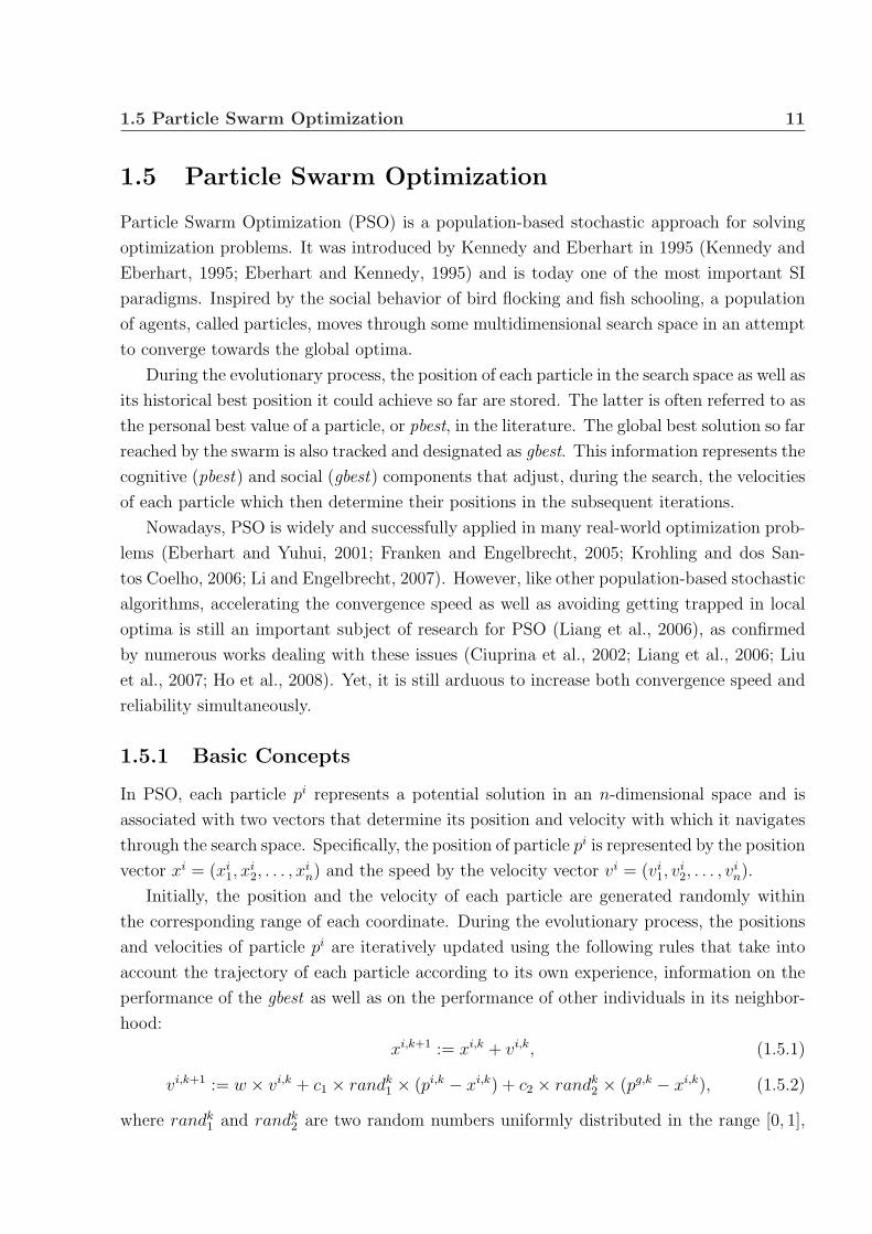
1.5 Particle Swarm Optimization
Particle Swarm Optimization (PSO) is a population-based stochastic approach for solving
optimization problems. It was introduced by Kennedy and Eberhart in 1995 (Kennedy and
Eberhart, 1995; Eberhart and Kennedy, 1995) and is today one of the most important SI
paradigms. Inspired by the social behavior of bird flocking and fish schooling, a population
of agents, called particles, moves through some multidimensional search space in an attempt
to converge towards the global optima.
During the evolutionary process, the position of each particle in the search space as well as
its historical best position it could achieve so far are stored. The latter is often referred to as
the personal best value of a particle, or pbest, in the literature. The global best solution so far
reached by the swarm is also tracked and designated as gbest. This information represents the
cognitive (pbest) and social (gbest) components that adjust, during the search, the velocities
of each particle which then determine their positions in the subsequent iterations.
Nowadays, PSO is widely and successfully applied in many real-world optimization prob-
lems (Eberhart and Yuhui, 2001; Franken and Engelbrecht, 2005; Krohling and dos San-
tos Coelho, 2006; Li and Engelbrecht, 2007). However, like other population-based stochastic
algorithms, accelerating the convergence speed as well as avoiding getting trapped in local
optima is still an important subject of research for PSO (Liang et al., 2006), as confirmed
by numerous works dealing with these issues (Ciuprina et al., 2002; Liang et al., 2006; Liu
et al., 2007; Ho et al., 2008). Yet, it is still arduous to increase both convergence speed and
reliability simultaneously.
1.5.1 Basic Concepts
In PSO, each particle pi represents a potential solution in an n-dimensional space and is
associated with two vectors that determine its position and velocity with which it navigates
through the search space. Specifically, the position of particle pi is represented by the position
vector xi = (xi1, x
i2, . . . , x
in) and the speed by the velocity vector vi = (vi
1, vi2, . . . , v
in).
Initially, the position and the velocity of each particle are generated randomly within
the corresponding range of each coordinate. During the evolutionary process, the positions
and velocities of particle pi are iteratively updated using the following rules that take into
account the trajectory of each particle according to its own experience, information on the
performance of the gbest as well as on the performance of other individuals in its neighbor-
hood:
xi,k+1 := xi,k + vi,k, (1.5.1)
vi,k+1 := w × vi,k + c1 × randk1 × (pi,k − xi,k) + c2 × randk
2 × (pg,k − xi,k), (1.5.2)
where randk1 and randk
2 are two random numbers uniformly distributed in the range [0, 1],

12 Introduction
w, c1 and c2 are parameters that represent the inertia weight, the cognition weight and the
social weight, respectively, xi,k and vi,k are the position and the velocity vectors of particle
pi in iteration k, respectively, pi,k is the pbest vector of particle pi in iteration k, and pg,k is
the gbest vector in iteration k. The classical PSO is illustrated in Algorithm 1.5.1, where N
denotes the size of the swarm and f(xi) represents the objective function value of particle
pi located at position xi.
Algorithm 1.5.1. PSO Pseudocode
1. Initialization. For each particle pi, i = 1, . . . , N , in the swarm, do thefollowing:1.1. Initialize xi and vi randomly.1.2. Evaluate f(xi).1.3. Initialize pbesti associated to pi.
2. Main loop. Repeat Steps 2.1 to 2.3 until a stopping criterion is met.2.1. Locate gbest.2.2. For each particle pi, set pbesti := xi if f(xi) ≤ f(pbesti).2.3. For each particle pi, update xi and vi by applying Equations (1.5.1) and(1.5.2), and evaluate f(xi).
1.5.2 PSO Variants and Improvements
PSO has rapidly gained popularity among researchers and is now a widely used optimizer
for practical problem solving. One of the first improvements made to PSO was related
to its strong parameter dependency. Indeed, one can find in the literature much work on
improving its performance via self-adaptation (Clerc, 1999; Shi and Eberhart, 2001; Yasuda
et al., 2003; Zhang et al., 2003) or by using hybrid techniques (Angeline, 1998b; Reynolds
et al., 2003; Higashi and Iba, 2003; Esquivel and Coello, 2003). Theoretical studies have
mainly focused on convergence and stability analysis (Clerc and Kennedy, 2002; Trelea,
2003; Kadirkamanathan et al., 2006; van den Bergh and Engelbrecht, 2006).
Hybridization of PSO with other techniques or evolutionary paradigms is also a very
active research trend. In order to increase diversity within the swarm and thus to avoid
premature convergence, many researchers have considered introducing operators inspired
from Genetic Algorithms (GA) within PSO, such as selection (Angeline, 1998b), crossover
(Chen et al., 2007) and mutation (Andrews, 2006). For instance, to include within PSO a
natural selection mechanism can help increasing the general fitness of the swarm at each
generation. It is explained by the fact that the selection mechanism allows the swarm to
change the current search area or to jump towards another one, which makes the algorithm
convergent faster (EL-Dib et al., 2004). EL-Dib et al. proposed to modify the positions and
the velocities of randomly selected particles using formulas inspired from the reproduction
system of species with the following crossover rules. Let x1 and x2 be the positions of two

1.6 Organization and Contributions 13
particles randomly selected (the parents), and let v1 and v2 be their respective velocities.
Then the positions and velocities of two created candidate particles (the offspring), denoted
x3, x4 and v3, v4, respectively, are determined by arithmetic crossover, for the position of
the offspring, and as the sum of the velocity vectors of the parents normalized to the original
length of each parent velocity vector, for the velocity:
x3 := r × x1 + (1− r)× x2,
x4 := r × x2 + (1− r)× x1,
v3 :=|v1|
|v1 + v2| × (v1 + v2),
v4 :=|v2|
|v1 + v2| × (v1 + v2),
where r is a random number from the interval [0, 1] and | · | is some vector norm.
Other variations include the incorporation of techniques such as local search (Liang and
Suganthan, 2005), cooperative approaches (van den Bergh and Engelbrecht, 2004) and DE
(Zhang and Xie, 2003). In (Zhang and Xie, 2003) for example, the hybridization of PSO
with DE is proposed to speed up the convergence. This method uses Equations (1.5.1) and
(1.5.2) at the odd iterations, while it uses the following mutation operation rule at the even
iterations with a trial point T i := pi:
If (rand < πc or n = k) then T i := pg + ~δ,
where k is a random integer chosen from [1, n], which ensures that at least one component will
eventually participate in the mutation, πc (≤ 1) is the crossover rate, pg is the gbest vector
and ~δ := (~∆1 + ~∆2)/2, where ~∆1 = pa− pb and ~∆2 = pc− pd represent the difference vectors
between two pbests pa and pb and two pbests pc and pd, respectively, selected randomly from
the pbest set. The resulting trial point T i replaces pi if its fitness value is better than the
fitness value of pi.
1.6 Organization and Contributions
In the subsequent chapters, we will describe the original EC methods that we have developed
to address the problem of the termination criteria. Our main objective is to demonstrate
that the novel mechanisms developed in this research can effectively provide the search
process with the ability to stop automatically, without external intervention. In addition,
we ensure that the automatic termination does not have a negative impact on the quality of
the solution obtained.

14 Introduction
In Chapter 2, we illustrate some of the main drawbacks of EC that have led us to develop
the Gene Matrix (GM). The GM, described in this chapter, is the core mechanism common to
our proposed methods in this study, and developed to equip the search with a termination
tool. We also describe the mutagenesis operator, a new type of mutation that works in
combination with the GM. Moreover, we overview the main concepts of the Nelder-Mead
(NM) method, a local search algorithm used to accelerate the search in the final stage of the
search process.
In Chapter 3, we introduce the Genetic Algorithms Combined with Accelerated Mutation
and Automatic Termination (G3AT) method. G3AT is the first method that is embedded
with the GM. The competitiveness of G3AT against existing methods is demonstrated and
the influence of the GM on the search is extensively analyzed.
In Chapter 4, an improvement of G3AT is presented. It addresses several drawbacks of
the GM by calling the novel Space Decomposition (SD) and Space Rotation (SR) mecha-
nisms. The enhanced method is named Genetic Algorithm with Automatic Termination and
Search Space Rotation (GATR). We show through extensive numerical experiments that the
solutions obtained do not suffer from premature termination and that GATR is comparable
or superior to many state-of-the-art EAs.
In Chapter 5, we show that the GM, SD and SR mechanisms can also be applied to
DE, as an illustration of another EA. We present the Differential Evolution with Automatic
Termination (DEAT) method and demonstrate that DEAT can also terminate the search
automatically and be equal or superior to other DE methods.
In Chapter 6, we combine the Principal Component Analysis (PCA) technique with
the GM and implement it on the PSO paradigm in order to compose the Automatically
Terminated Particle Swarm Optimization with Principal Component Analysis (AT-PSO-
PCA) method. The performance of AT-PSO-PCA is discussed through several numerical
experiments and the impact of PCA is analyzed.
Finally, Chapter 7 summarizes the main contributions of this dissertation and discusses
possible opportunities for further research.

Chapter 2
Gene Matrix, Mutagenesis andIntensification
The novel EC methods that we propose in this study are equipped with new directing
strategies. The common elements are the Gene Matrix (GM), the mutagenesis operator and
the final intensification process. The GM is a matrix constructed to represent subranges of
the possible values of each variable and consequently reflects the distribution of the genes over
the search range. Its role is to assist the exploration process in two different ways. First, the
GM can provide the search with new diverse solutions by applying the mutagenesis operator.
The mutagenesis operator is a new type of mutation that works in combination with the GM.
It alters some individuals in order to accelerate the exploration and exploitation processes
by guiding the search specifically towards unexplored areas. Also, the GM is the key to let
the search know how far the exploration process has been performed in order to determine
an adequate termination instant. To further accelerate the search process, a local search
method is used in the final intensification process to improve the best candidate solution
obtained upon GM termination.
In this chapter, the concepts of premature convergence and slow convergence are re-
viewed, before providing an overview of the commonly adopted termination criteria in EC.
Then, the advantages of having automatic termination criteria are discussed. Finally, the
GM, the mutagenesis operator as well as the Nelder-Mead local search method are described
in detail.
2.1 Premature Convergence
When the diversity of the population decreases below a certain level, the population may
converge to a suboptimal similar individual. EC techniques have been initially designed so
that they can focus their search on promising areas of the search space discovered during
the exploration phase. Consequently, diversity among individuals of the population tends to

16 Gene Matrix, Mutagenesis and Intensification
Figure 2.1: Objective function evolution at different stages of the search.
decrease and to concentrate around individuals with high fitness (Fogel, 1994). As a result
of this behavior, EC techniques tend to get trapped in the vicinity of local optima. This
phenomenon is known as “premature convergence”.
2.2 Slow Convergence
Figure 2.1 depicts the objective function evolution for a minimization problem at three dif-
ferent stages of the search (Eiben and Smith, 2003). At the first stage, represented in Figure
2.1(a), the population is randomly distributed over the search space. As the evolutionary
search progresses, the population tends to concentrate around valleys, as depicted in Figure
2.1(b). At the end of the search, the whole population lies on a few valleys as shown in
Figure 2.1(c). Hopefully, the individuals are gathering around a global optimum.
However, Figure 2.2 characterizes the convergence behavior of an evolutionary search by

2.3 Automatic Termination 17
Figure 2.2: Convergence behavior of an evolutionary search.
plotting the best value of the objective function in time. We can observe a rapid descendant
progression of the objective value during the beginning of the search. Later on, progresses in
terms of objective value deteriorate and it could be insignificant to let the search run after
a certain time. As a result, compared to local search techniques, EC methods suffer from
slow convergence. Indeed, due to their random constructions, they do not exploit much local
information to guide their search. Typically, these techniques cover a large frontier in the
search space in the early stage of the search but explore it in a less directional approach.
Thus when dealing with stopping criteria, one should also pay meticulous attention to the
balance between exploration and exploitation.
2.3 Automatic Termination
Basically, EC methods cannot decide when or where they can terminate the search and usu-
ally a user should prespecify the maximum number of generations or function evaluations
as termination criteria. There are only a few recent works on termination criteria for EAs
(Giggs et al., 2006; Kwok et al., 2007; Jain et al., 2001). In (Giggs et al., 2006), an empirical
study is conducted to detect the maximum number of generations using the problem char-
acteristics. In (Kwok et al., 2007), the particle swarm optimization algorithm is stopped
using a termination condition based on statistics. The hypothesis testing non-parametric
sign-test method is considered as a decision making process using a list of the stored highest
fitness values in each iteration. The search stops when the hypothetical test indicates that
no significant improvement in terms of solution quality is going to occur. In (Jain et al.,
2001), eight termination criteria have been studied with an interesting idea of using clus-
tering techniques to examine the distribution of individuals in the search space at a given
generation.
The most commonly employed termination criteria for EC methods can be enumerated
as the TFit Criterion, the TPop Criterion, the TBud Criterion and the TSFB Criterion. The
18 Gene Matrix, Mutagenesis and Intensification
TFit Criterion uses convergence measures of the best fitness function values over generations.
This criterion is used for instance in (Hansen and Kern, 2004; Tsai et al., 2004; Zhong et al.,
2004; Ong et al., 2006), where the goal is to get as close as possible to the known global
minima. In (Leung and Wang, 2001), the search stops after reaching the maximum number
of consecutive generations without improvement. When used alone, however, TFit Criterion
may easily lead the search towards local minima, especially if the algorithm tends to reach in
early stages a deep local minimum (Jain et al., 2001; Safe et al., 2004; Hedar and Fukushima,
2006b). The TPop Criterion uses convergence measures of the population over generations.
This criterion is not particularly efficient though, since having one individual to reach a global
minimum is enough. Moreover making the whole population or a part of it convergent can
be expensive. The TBud Criterion uses a prespecified budget, that can be the number of
generations or function evaluations (Yao et al., 1999; Lee and Yao, 2004; Ong and Keane,
2004; Tu and Lu, 2004; Koumousis and Katsaras, 2006; Ong et al., 2006; Zhou et al., 2007).
The drawback is that it requires prior information about the test problem and is also highly
problem dependent. Finally, the TSFB Criterion checks the progress of the exploration and
exploitation processes by using search feedback measures. Unfortunately, the use of search
feedback may bring a complexity problem due to the need to save and check historical search
information that can be huge and is also very sensitive to the dimensionality.
Good automatic termination criteria should assure that the search avoids premature
termination but also indicates the point in time when further computations becomes un-
necessary. This feature is of key importance in some real-world applications such as in
“evolutionary testing” (O’Sullivan et al., 1998; McMinn, 2004). Indeed, during the develop-
ment of embedded systems, testing is one of the most important quality assurance measure.
A huge amount of effort and budget is allocated for testing. In evolutionary testing, EAs are
used for test data generation and to verify the logical and temporal correctness of a system.
Most testing methods are specialized in the logical correctness. However, for real-time sys-
tems, it is also essential to check the temporal correctness. Evolutionary testing fills this gap
by testing the timing constraints where a temporal error occurs when outputs are produced
too early or if the computational time is too long. In such situations, it is crucial to have
reliable automatic termination criteria for EAs.
Multi-start methods may also benefit from automatic termination criteria. Among the
main components of a multi-start method, we note the stopping criterion used within the
generation mechanism of candidate solutions. The stopping criterion, in this case also re-
ferred to as the restarting criterion, is prespecified by the user and has a big impact on the
overall computational cost of the method. Consequently, a reliable automatic termination
criterion may have a positive effect on multi-start methods, by reducing the cost of gener-
ating candidate solutions, thereby more iterations can be allowed with a fixed budget. In
the same way, automatic termination criteria may also be used effectively for dynamic EA

2.4 Gene Matrix and Termination 19
(Koo et al., 2010) where the convergence is very dependent on the behavior of the dynamic
problem.
2.4 Gene Matrix and Termination
To achieve a wide exploration and to keep track of the progress of the exploration, we propose
the concept of the GM. Each individual x in the search space consists of n variables. The
range of each variable is divided into m sub-ranges in order to check the diversity of the
variable values. Then, we define a solution counter matrix C of size n×m, in which entry cij
represents the number of generated solutions such that the i-th variable lies in the sub-range
j, where i = 1, . . . , n, and j = 1, . . . , m. The GM is initialized to be the n×m zero matrix
in which each entry of the i-th row refers to a sub-range of the i-th variable. GM is a 0–1
matrix and while the search is processing, the entries of GM are updated from zeros to ones
if new values for variables are generated within the corresponding sub-ranges. After having a
GM full, i.e., with no zero entry, the search learns that an advanced exploration process has
been achieved and is stopped. In this way, the principal use of the GM is to equip the search
process with a practical termination tool. Moreover, the GM assists in providing the search
with diverse solutions as will be shown in Subsection 2.4.1. By keeping track of explored
area of the search space in order to concentrate on parts that have not been considered yet,
the GM yields some similarities with tabu search ideas (Glover, 1986; Ting et al., 2009). We
define the GM completion ratio, referred to as CP , as the number of non-null entries divided
by the total number of entries of GM. We have considered two types of GM as follows.
Simple Gene Matrix (GMS)
GMS does not take into account the number of solutions lying within each sub-range. During
the search, the solution counter matrix C is updated. Let xi be the representation of the
i-th variable, i = 1, . . . , n. Once variable i gets a value corresponding to a non-explored sub-
range j, i.e., cij > 0, then GM is updated by flipping the zero into one in the corresponding
(i, j) entry. Therefore, the updating process for GMS can be defined as
(GMS)ij =
{0, if cij = 01, if cij > 0,
(2.4.1)
where i = 1, . . . , n, j = 1, . . . , m, and (GMS)ij is the (i, j) entry of the gene matrix GMS.
Figure 2.3 shows an example of GMS in two dimensions, i.e., n = 2. In this figure, the
range of each variable is divided into ten sub-ranges. We can see that for the first gene x1, no
individual has been generated inside the sub-ranges 1, 7 and 10, i.e., c1,1 = c1,7 = c1,10 = 0.
Consequently, the (1, 1), (1, 7) and (1, 10) entries of GMS are equal to zero. For the second

20 Gene Matrix, Mutagenesis and Intensification
Figure 2.3: An example of the GM in R2.
gene x2, only the first and the last sub-ranges are unvisited, hence entries (2, 1) and (2, 10)
of GMS are null.
Advanced Gene Matrix (GMAα)
GMAα comes along with a ratio α predefined by the user. Unlike GMS, GMA
α is not immedi-
ately updated, unless the ratio of the number of individuals that have been generated inside
a sub-range and m equals or exceeds α. Therefore, the updating process for GMAα can be
defined as
(GMAα )ij =
{0, if cij < αm1, if cij ≥ αm,
(2.4.2)
where i = 1, . . . , n, j = 1, . . . , m, and (GMAα )ij is the (i, j) entry of the gene matrix GMA
α .
An example of GMAα with α = 0.2 in two dimensions can be found in Figure 2.3. Like
GMS, no individual has been generated inside sub-ranges 1, 7 and 10 for gene x1. However,
unlike GMS, entry (1, 3) is equal to 0 in GMA0.2 since there is only one individual lying inside
the third sub-range, that is, c1,3 = 1 < αm = 2. For the same reason, x2 has six zero-entries
corresponding to six sub-ranges in which the number of generated individuals divided by m
is less than α. This example refers to the first generation of individuals. In a succeeding
generation, if one or more individuals are generated inside the third sub-range for x1 for
example, then entry (1, 3) will be set equal to one.
2.4 Gene Matrix and Termination 21
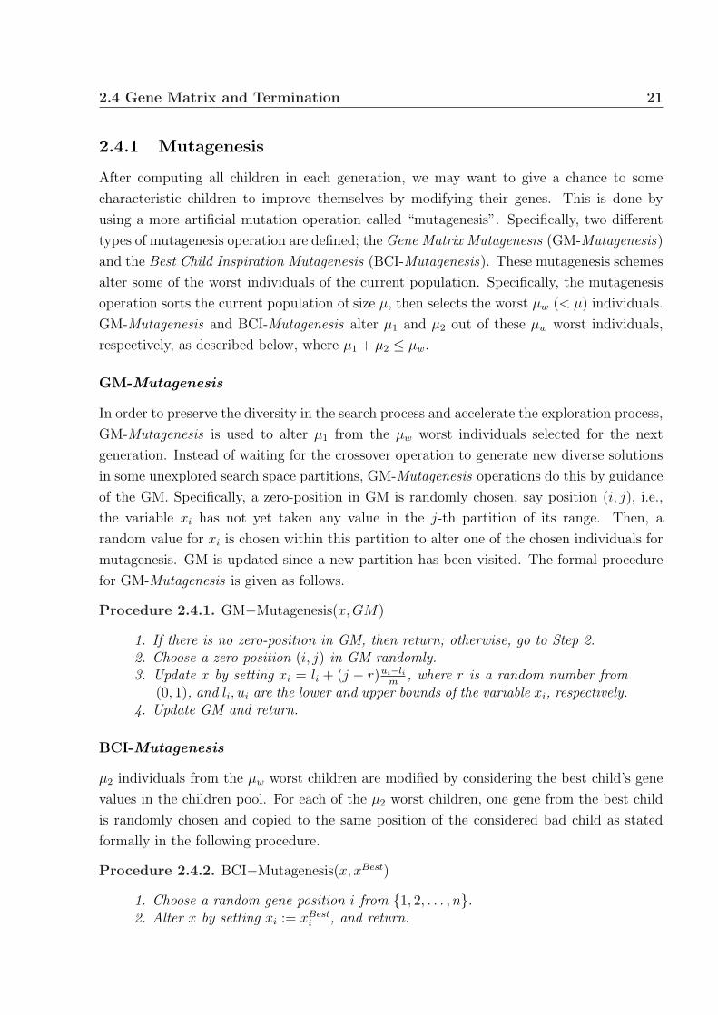
2.4.1 Mutagenesis
After computing all children in each generation, we may want to give a chance to some
characteristic children to improve themselves by modifying their genes. This is done by
using a more artificial mutation operation called “mutagenesis”. Specifically, two different
types of mutagenesis operation are defined; the Gene Matrix Mutagenesis (GM-Mutagenesis)
and the Best Child Inspiration Mutagenesis (BCI-Mutagenesis). These mutagenesis schemes
alter some of the worst individuals of the current population. Specifically, the mutagenesis
operation sorts the current population of size µ, then selects the worst µw (< µ) individuals.
GM-Mutagenesis and BCI-Mutagenesis alter µ1 and µ2 out of these µw worst individuals,
respectively, as described below, where µ1 + µ2 ≤ µw.
GM-Mutagenesis
In order to preserve the diversity in the search process and accelerate the exploration process,
GM-Mutagenesis is used to alter µ1 from the µw worst individuals selected for the next
generation. Instead of waiting for the crossover operation to generate new diverse solutions
in some unexplored search space partitions, GM-Mutagenesis operations do this by guidance
of the GM. Specifically, a zero-position in GM is randomly chosen, say position (i, j), i.e.,
the variable xi has not yet taken any value in the j-th partition of its range. Then, a
random value for xi is chosen within this partition to alter one of the chosen individuals for
mutagenesis. GM is updated since a new partition has been visited. The formal procedure
for GM-Mutagenesis is given as follows.
Procedure 2.4.1. GM−Mutagenesis(x, GM)
1. If there is no zero-position in GM, then return; otherwise, go to Step 2.2. Choose a zero-position (i, j) in GM randomly.3. Update x by setting xi = li + (j − r)ui−li
m, where r is a random number from
(0, 1), and li, ui are the lower and upper bounds of the variable xi, respectively.4. Update GM and return.
BCI-Mutagenesis
µ2 individuals from the µw worst children are modified by considering the best child’s gene
values in the children pool. For each of the µ2 worst children, one gene from the best child
is randomly chosen and copied to the same position of the considered bad child as stated
formally in the following procedure.
Procedure 2.4.2. BCI−Mutagenesis(x, xBest)
1. Choose a random gene position i from {1, 2, . . . , n}.2. Alter x by setting xi := xBest
i , and return.

22 Gene Matrix, Mutagenesis and Intensification
2.5 Nelder-Mead Method
The methods proposed in this research invoke a local search (LS) method at the end of the
search to produce an improved final solution from the best solution found upon automatic
termination. The LS method used in our methods is based on the Nelder-Mead method
(Nelder and Mead, 1965). The Nelder-Mead method is a derivative-free nonlinear optimiza-
tion method. To avoid the computation of the derivative information for minimizing an
objective function of several variables, this local search method uses the concept of a sim-
plex. A simplex is the convex hull of a set of n+1 vertices, x1, x2, . . . , xn+1 in n dimensions;
the geometric figure of nonzero volume is for instance a line segment on a line or a triangle
on a plane.
At each iteration, the Nelder-Mead method maintains a non-degenerate simplex, i.e., a
generalized triangle in n dimensions, as well as the function value of each vertex. Typically,
new points (and their function values) are computed by reflecting the worst point through
the remaining points considered as a plane. Then, the new worst point is replaced to form
a new simplex. A sequence of simplex is thus created and the function value at each vertex
decreases.
In order to create a sequence of simplices, some rules are applied; reflection, expansion,
contraction and shrinkage. They possess the coefficients ρ, χ, γ and σ, respectively, such
that:
ρ > 0, χ > 1, 0 < γ < 1, 0 < σ < 1.
Let B = (x1, y1), G = (x2, y2) and W = (x3, y3) be the three vertices of a triangle as
in (Mathews and Fink, 2004). Given f(x, y), the function to be minimized, let us evaluate
each vertices and order them such that f(B) ≤ f(G) ≤ f(W ). With this notation, point B
conveniently stands for “best”, G for “good” and W for “worst”. M is the midpoint between
B and G:
M =B + G
2=
(x1 + x2
2,y1 + y2
2
).
2.5.1 Reflection
If the function value decreases while moving along the vertex from W to B and from W to
G, then the algorithm computes a test point R located on the opposite side from W of the
line joining B and G as in Figure 2.4. Specifically, R = 2M −W is found by reporting the
length d of the line segment joining W and M and extending the same distance from M on
the opposite side.

2.5 Nelder-Mead Method 23
Figure 2.4: Reflection point for a simplex in two dimensions.
Figure 2.5: Expansion point for a simplex in two dimensions.
2.5.2 Expansion
If the vertex R has a function value smaller than B, then R is extended again through the
line segment between W and R by the distance d from R to reach the point E = 2R −M
as in Figure 2.5.
2.5.3 Contraction
Contraction is used when the computed point R is not better than G. When it happens,
the algorithm generates two points C1 and C2 located on the line segment WR and WM ,
with C1 inside the triangle BGW and C2 inside the triangle BRG as drawn in Figure 2.6.
Afterwards, the algorithm tries to locate between C1 and C2 a point C that would be better
than R and W . If such point is found, it becomes the new point to be tested instead of R.
2.5.4 Shrinkage
After contraction, if the function value of the vertex C is bigger than W , then W and G are
moved closer to B. This is achieved by replacing them by two new points S and M located
in the middle of the line segments WB and GB, respectively, as depicted in Figure 2.7.

24 Gene Matrix, Mutagenesis and Intensification
Figure 2.6: Contraction points for a simplex in two dimensions.
Figure 2.7: Shrinkage points for a simplex in two dimensions.
2.5.5 Kelley’s Modification
It has been shown that the Nelder-Mead method can stagnate and converge to a non-
optimal point, even for very simple problems (Mckinnon, 1999). Nevertheless, under certain
conditions, convergence of the Nelder-Mead method to a stationary point can be guaranteed.
Indeed, Kelley (Kelley, 1999) proposes a test for sufficient decrease and this modification of
the Nelder-Mead method is the one we employ in the final stage of our proposed methods.

Chapter 3
Genetic Algorithms Combined withAccelerated Mutation and AutomaticTermination
EAs are general problem solvers that show powerful performance in solving various problems.
There have been many attempts to enhance the structure of EAs. However, EAs still have
no automatic termination criterion. This chapter introduces our first attempt to equip GA,
as an example of EAs, with new automatic termination criteria and acceleration elements.
The proposed method is called Genetic Algorithm with Accelerated Automatic Termination
(G3AT). In the G3AT method, the GM is constructed to equip the search process with a
self-check to judge how much exploration has been done and to maintain the population
diversity. Moreover, the mutagenesis operation is used to achieve more efficient and faster
exploration and exploitation processes. The computational experiments show the efficiency
of the G3AT method with the proposed termination criteria and the mutagenesis operation.
3.1 Introduction
In this chapter, we introduce a new hybrid GA that implements an automatic TSFB termi-
nation criterion (see Section 2.3) with low complexity structure. Specifically, a new version
of GAs called G3AT is proposed. In the G3AT method, a new GA method is designed
and equipped with automatic termination criteria and new accelerating elements in order to
achieve better performances.
The G3AT method is composed by modifying GAs with some directing strategies. First,
an exploration and exploitation scheme is invoked to equip the search process with acceler-
ated automatic termination criteria. Specifically, this role is carried out by the GM. The role
of GM is to assist the exploration process in two different ways. First, GM can provide the
search with new diverse solutions by applying the mutagenesis operator. The mutagenesis

26Genetic Algorithms Combined with Accelerated Mutation and Automatic
Termination
operator alters some survival individuals in order to accelerate the exploration and exploita-
tion processes. In addition, GM is used to let G3AT know how far the exploration process
has gone in order to judge a termination point. The mutagenesis operation lets G3AT behave
like a so-called “Memetic Algorithm” (Moscato, 1999) in order to achieve faster convergence
(Ong and Keane, 2004; Ong et al., 2006). The numerical results presented later show that
mutagenesis is effective and much cheaper than a local search. Then, the final intensification
process can be started in order to refine the elite solutions obtained so far. The numerical
results indicate that the proposed G3AT method is competitive with some other versions of
GAs.
The rest of this chapter is structured as follows. In Section 3.2, we highlight and describe
the main components of the G3AT method. The formal algorithm of G3AT is also provided
in this section. In Section 3.3, numerical experiments aiming at analyzing the performance
of G3AT and its novel operators are discussed. The effects that have GM and mutagenesis
on the algorithm is also examined. Numerical comparisons with several advanced GAs and
state-of-art EAs are carried out in Section 3.4. Section 3.5 contains a comparison between
G3AT and the GA included in the MATLAB toolbox. Finally, the conclusion makes up
Section 3.6.
3.2 G3AT Mechanisms
In this section, a new modified version of GAs called G3AT is presented. Before presenting
the details of G3AT, we highlight some remarks on GAs to motivate the proposed G3AT.
Keeping diversity and elitism is an important issue in GAs. A key factor in composing
GAs is to define genetic operators that can maintain the balance between diversity and
elitism. Those considerations lead us to compose the mutagenesis operator. Mutagenesis
alters some survival individuals while maintaining diversity and elitism and accelerates the
diversification and intensification processes.
EAs are not equipped with automatic termination criteria. Actually, EAs may obtain
an optimal or near-optimal solution in an early stage of the search but they are not learned
enough to judge whether they can terminate. To counter this weakness, G3AT is built
with termination measures that can check the progress of the exploration process through
successive generations. Then, an exploitation process refines the best candidates obtained
so far in order to achieve faster convergence.
In designing G3AT, we have considered the above-mentioned remarks. The standard
GA is modified with the Simple GM and termination mechanisms, described in Section 2.4.
The selection, crossover and mutation operators that compose G3AT are described in this
section.

3.2 G3AT Mechanisms 27
Figure 3.1: An example of the crossover operation.
3.2.1 Parent Selection
The parent selection mechanism first produces an intermediate population P ′ from the initial
population P , i.e., P ′ ⊆ P , as in the canonical GA. For each generation, P ′ has the same size
as P but an individual can be present in P ′ more than once. The individuals in P are ranked
with their fitness function values based on the linear ranking selection mechanism (Baker,
1985; Hedar and Fukushima, 2003). Indeed, individuals in P ′ are copies of individuals in
P depending on their fitness ranking; the higher fitness an individual has, the more the
probability that it will be copied is. This process is repeated until P ′ is full while an already
chosen individual is not removed from P .
3.2.2 Crossover
The crossover operation has an exploration tendency, and therefore it is not applied to all
parents. First, for each individual in the intermediate population P ′, the crossover operation
chooses a random number from the interval (0, 1). If the chosen number is less than a
prespecified crossover probability πc ∈ (0, 1), the individual is added to the parent pool.
After that, two parents from the parent pool are randomly selected and mated to produce
two children c1 and c2, which are then placed in the children pool. These procedures are
repeated until all parents are mated. The crossover operator used in G3AT method is a
ρ-point operator with random ρ ≤ n. Therefore, a recombined child is calculated to have ρ
partitions. Both parents genotypes are cut in ρ partitions and the randomly chosen parts are
exchanged to create two children. Let us note that a parent is selected only once, and if the
total number of parents inside the parent pool is uneven, then the last parent that was added
into the pool is not considered for the mating procedure. As an example, Figure 3.1 shows
two parents p1 and p2 partitioned into five partitions at the same positions (after the second,
third, fourth and sixth genes). Then, a recombined child c1 is generated to inherit partitions
from the two parents according to a random sequence of zeros and ones, (0, 0, 1, 0, 1) in this
example, meaning that its first, second and fourth partitions will be inherited from p1 and
third and fifth partitions from p2. The other partition sequence of the recombined child c2
is the complementary of the sequence of c1, namely (1, 1, 0, 1, 0). The following procedure
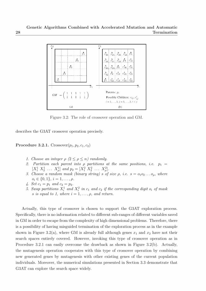
28Genetic Algorithms Combined with Accelerated Mutation and Automatic
Termination
Figure 3.2: The role of crossover operation and GM.
describes the G3AT crossover operation precisely.
Procedure 3.2.1. Crossover(p1, p2, c1, c2)
1. Choose an integer ρ (2 ≤ ρ ≤ n) randomly.2. Partition each parent into ρ partitions at the same positions, i.e. p1 =
[X11 X1
2 . . . X1ρ ] and p2 = [X2
1 X22 . . . X2
ρ ].3. Choose a random mask (binary string) s of size ρ, i.e. s = o1o2 . . . oρ, where
oi ∈ {0, 1}, i = 1, . . . , ρ.4. Set c1 = p1 and c2 = p2.5. Swap partitions X1
i and X2i in c1 and c2 if the corresponding digit oi of mask
s is equal to 1, where i = 1, . . . , ρ, and return.
Actually, this type of crossover is chosen to support the G3AT exploration process.
Specifically, there is no information related to different sub-ranges of different variables saved
in GM in order to escape from the complexity of high dimensional problems. Therefore, there
is a possibility of having misguided termination of the exploration process as in the example
shown in Figure 3.2(a), where GM is already full although genes x1 and x2 have not their
search spaces entirely covered. However, invoking this type of crossover operation as in
Procedure 3.2.1 can easily overcome the drawback as shown in Figure 3.2(b). Actually,
the mutagenesis operation cooperates with this type of crossover operation by combining
new generated genes by mutagenesis with other existing genes of the current population
individuals. Moreover, the numerical simulations presented in Section 3.3 demonstrate that
G3AT can explore the search space widely.

3.2 G3AT Mechanisms 29
3.2.3 Mutation
The mutation operator uses information contained in GM. For each individual in the in-
termediate population P ′ and for each gene, a random number from the interval (0, 1) is
associated. If the associated number is less than a prespecified mutation probability πm,
then the individual is copied to the intermediate pool IPM . The number of times the as-
sociated numbers are less than the mutation probability πm is counted. Let numm denote
this number. Afterward, the mutation operation makes sure that the total number numm
of genes to be mutated does not exceed the number of zeros in the GM, denoted numzeros.
Otherwise, the number of genes to be mutated is reduced to numzeros. Finally, a zero from
GM is randomly selected, say in position (i, j), and a randomly chosen individual from IPM
has its gene xi modified by a new value lying inside the j-th partition of its range. The
formal procedure for mutation is analogous to Procedure 2.4.1.
Procedure 3.2.2. Mutation(x,GM)
1. If GM is full, then return; otherwise, go to Step 2.2. Choose a zero-position (i, j) in GM randomly.3. Update x by setting xi = li + (j − r)ui−li
m, where r is a random number from
(0, 1), and li, ui are the lower and upper bounds of the variable xi, respectively.4. Update GM and return.
3.2.4 G3AT Formal Algorithm
G3AT starts with an initial population of size µ. As in a standard GA, G3AT evaluates
the population members, and then, parent selection, crossover and mutation operations are
applied to generate the offspring. Following memetic algorithm features, G3AT invokes a
local search method to improve some promising children. Since applying a local search
might be expensive, G3AT alternatively uses mutagenesis operation. Therefore, to avoid the
redundance of applying two intensification schemes for the same purpose, either the local
search step or the mutagenesis step is invoked. This pattern is repeated until the termination
criteria are satisfied. Specifically, G3AT is terminated when η generations have elapsed after
getting a full GM. The reason for waiting η generations after having a full GM is to allow
the crossover operation, which is the main exploration operation, to explore corresponding
partitions found by the last update of GM. It is worthwhile to mention that the main role
of GM is to guide the search process towards unexplored regions, not to explore them since
the exploration is the main role of the crossover operation. Finally, G3AT uses a complete
local search method as final intensification in order to refine the best solutions found so far.
The formal detailed description of G3AT is given in the following algorithm.
Algorithm 3.2.3. G3AT Algorithm

30Genetic Algorithms Combined with Accelerated Mutation and Automatic
Termination
1. Initialization. Set values of m, µ, η, and (li, ui), for i = 1, . . . , n. Set thecrossover and mutation probabilities πc ∈ (0, 1) and πm ∈ (0, 1), respectively.Set the generation counter t := 0. Initialize GM as an n × m zero matrix,and generate an initial population P0 of size µ.
2. Parent Selection. Evaluate the fitness function F of all individuals in Pt.Select an intermediate population P ′
t from the current population Pt.
3. Crossover. Associate a random number from (0, 1) with each individual inP ′
t and add this individual to the parent pool SPt if the associated number isless than πc. Repeat Steps 3.1 and 3.2 until all chosen parents from SPt aremated.3.1. Choose two parents p1 and p2 from SPt. Mate p1 and p2 using Procedure3.2.1 to reproduce children c1 and c2.3.2. Update the children pool SCt by SCt := SCt ∪ {c1, c2}, update SPt bySPt := SPt \ {p1, p2}, and update GM.
4. Mutation. Associate a random number from (0, 1) with each gene for eachindividual in P ′
t . Mutate the individuals which have an associated numberless than πm by applying Procedure 3.2.2. Add the mutated individual to thechildren pool SCt, and update GM.
5. Local Search. Apply a local search method to improve the best child (ifexists), and then update GM.
6. Stopping Condition. If η generations have passed after getting a full GM,then go to Step 9. Otherwise, go to Step 7.
7. Survivor Selection. Evaluate the fitness function of all generated childrenSCt, and choose the µ best individuals in Pt ∪ SCt for the next generationPt+1.
8. Mutagenesis. Apply Procedures 2.4.1 and 2.4.2 to alter the µw worstindividuals in Pt+1, set t := t + 1, update GM, and go to Step 2.
9. Intensification. Apply a local search method starting from each solutionfrom the µelite elite ones obtained in the previous search stage.
There are three main versions of Algorithm 3.2.3. These versions are composed by
considering only one intensification scheme; mutagenesis or Local Search (Step 5 or Step 8).
G3ATL version is composed by invoking Local Search and discarding Step 8, while G3ATSM
and G3ATAM discard Step 5 and invoke mutagenesis using Simple and Advanced GM (see
Section 2.4), respectively. Actually, the main difference between the local search version
G3ATL and mutagenesis versions G3ATSM and G3ATA
M is that the latter replaces the exact
local search method with the defined heuristic local search mutagenesis. The difference
between an exact local search method with a heuristic local search is that the former has
a convergence guarantee under tractable time while the latter does not (Noman and Iba,
2005). Therefore, G3ATL, G3ATSM and G3ATA
M can be considered as memetic algorithms or
hybrid global-local search algorithms. The difference in these proposed algorithms is the use
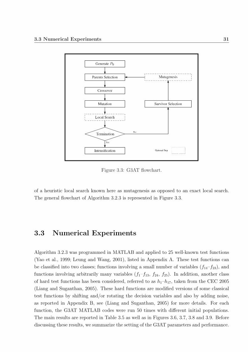
3.3 Numerical Experiments 31
Figure 3.3: G3AT flowchart.
of a heuristic local search known here as mutagenesis as opposed to an exact local search.
The general flowchart of Algorithm 3.2.3 is represented in Figure 3.3.
3.3 Numerical Experiments
Algorithm 3.2.3 was programmed in MATLAB and applied to 25 well-known test functions
(Yao et al., 1999; Leung and Wang, 2001), listed in Appendix A. These test functions can
be classified into two classes; functions involving a small number of variables (f14–f23), and
functions involving arbitrarily many variables (f1–f13, f24, f25). In addition, another class
of hard test functions has been considered, referred to as h1–h17, taken from the CEC 2005
(Liang and Suganthan, 2005). These hard functions are modified versions of some classical
test functions by shifting and/or rotating the decision variables and also by adding noise,
as reported in Appendix B, see (Liang and Suganthan, 2005) for more details. For each
function, the G3AT MATLAB codes were run 50 times with different initial populations.
The main results are reported in Table 3.5 as well as in Figures 3.6, 3.7, 3.8 and 3.9. Before
discussing these results, we summarize the setting of the G3AT parameters and performance.

32Genetic Algorithms Combined with Accelerated Mutation and Automatic
Termination
Table 3.1: G3AT Parameter SettingParameter Definition Valueµ Population size min{50, 10n}πc Crossover probability 0.6πm Mutation probability 0.1m No. of GM columns 50nµ1 No. of individuals used by GM-Mutagenesis 2µ2 No. of individuals used by BCI-Mutagenesis 2µelite No. of starting points for intensification 1α Advanced GM percentage for G3ATA
M 3/mNMmaxIt No. of maximum iterations used by Local Search in G3ATL 5n
3.3.1 Parameter Setting
First, the search domain for Problem (1.1.1) is defined as
[L, U ] = {x ∈ Rn : li ≤ xi ≤ ui, i = 1, . . . , n} .
This search domain is essential for constructing the GM and it can be easily determined
for many application problems. However, the construction of the GM can be modified if
the actual search domain is not specified. The user can start with a sufficiently large initial
search domain and then new partitions of the GM can be added whenever new regions are
reached outside the initial search domain.
In Table 3.1, we summarize all G3AT parameters with their assigned values. These values
are based on the common setting in the literature or determined through our preliminary
numerical experiments.
We used the scatter search diversification generation method (Laguna and Marti, 2003;
Hedar and Fukushima, 2006a) to generate the initial population P0 of G3AT. In that method,
the interval [li, ui] of each variable is divided into four sub-intervals of equal size. New points
are generated and added to P0 as follows.
1. Choose one sub-interval for each variable randomly with a probability inversely pro-
portional to the number of solutions previously chosen in this sub-interval.
2. Choose a random value for each variable that lies in the corresponding selected sub-
interval.
We tested three mechanisms for local search in the intensification process based on two
methods; the Kelley’s modification (Kelley, 1999) of the Nelder-Mead (NM) method (Nelder
and Mead, 1965), and a MATLAB function named “fminunc.m”. These mechanisms are
1. method1: to apply 10n iterations of Kelley-NM method,

3.3 Numerical Experiments 33
Table 3.2: Results of Local Search Strategies
f n
f18 2f19 3f15 4f2 30f9 30
Initial Local Search Strategyf fmethod1 fmethod2 fmethod3
46118 371.3246 23.8734 13.0660–0.9322 –2.6361 –2.8486 –3.66958.8e+5 1998.5 0.0120 0.03092.2e+20 1.2+e19 1.1e+13 340.6061551.7739 256.0628 91.5412 193.4720
2. method2: to apply 10n iterations of MATLAB fminunc.m function, and
3. method3: to apply 5n iterations of Kelley-NM method, then apply 5n iterations of
MATLAB fminunc.m function.
Five test functions shown in Table 3.2 were chosen to test these three mechanisms. One
hundred random initial points were generated in the search space of each test function.
Then the three local search mechanisms were applied to improve the generated points. The
average results are reported in Table 3.2. The last mechanism method3 could improve the
initial values significantly and is better than the other two mechanisms. Therefore, G3AT
employs method3 for the local search in Step 4 of Algorithm 3.2.3. Moreover, method3 was
used with a bigger number of iterations as the final intensification method in Step 9 of
Algorithm 3.2.3.
For the parameter m, several preliminary numerical experiments have been done to set
its value and check its sensitivity. In these preliminary numerical experiments, different
values of m were tested and some of them are shown in Figure 3.4. Three terminations
were applied for each test problem; at m = 10n, m = 30n and m = 50n. Figure 3.4 shows
that premature termination has clearly occurred with m = 10n. We can observe that this
parameter is not sensitive for small changes but setting it equal to too small a value may lead
to premature termination. The best problem-free value found was m = 50n. Actually, no
further significant exploration of the search domains of the tested functions can be expected
for m > 50n.
It is worthwhile to mention that the extra cost for maintaining GM and applying muta-
genesis, which is not required in the standard GA, is still within a polynomial time of the
population size (µ), the variable dimension (n) and the maximum number of generations
(Gmax). Actually, mutagenesis is O(Gmax) and GM updating is O(µnGmax) for a whole run
of G3ATSM .
3.3.2 G3AT Performance
Extensive numerical experiments were carried out to examine the efficiency of G3AT and to
give an idea on how it works. First, several preliminary experiments were done to analyse

34Genetic Algorithms Combined with Accelerated Mutation and Automatic
Termination
0 50 100 150 200 250 300 350−14000
−12000
−10000
−8000
−6000
−4000
−2000
0
Generations
Fun
ctio
n V
alue
sf8
Ful
l GM
(m
= 1
0n)
Ter
min
atio
n
Ful
l GM
(m
= 3
0n)
Ter
min
atio
n
Ful
l GM
(m
= 5
0n)
Ter
min
atio
n
0 5 10 15 20 25 30 350
20
40
60
80
100
120
140
160
180
200
Generations
Fun
ctio
n V
alue
s
f18
Ful
l GM
(m
= 1
0n)
Ter
min
atio
n
Ful
l GM
(m
= 3
0n)
Ter
min
atio
n
Ful
l GM
(m
= 5
0n)
Ter
min
atio
n
0 10 20 30 40 50 60−3.5
−3
−2.5
−2
−1.5
−1
−0.5
Generations
Fun
ctio
n V
alue
s
f20
Ful
l GM
(m
= 1
0n)
Ter
min
atio
n
Ful
l GM
(m
= 3
0n)
Ter
min
atio
n
Ful
l GM
(m
= 5
0n)
Ter
min
atio
n
Figure 3.4: Tuning of the number of GM columns m.

3.3 Numerical Experiments 35
G3AT operations and some of them are summarized in Figure 3.5 and Table 3.3. Each graph
of Figure 3.5 shows the results of the following three algorithms:
• G3ATSM , which is G3AT with mutagenesis and Simple GM.
• G3ATSM without mutagenesis, i.e., GA with the crossover and mutation operations
stated in Procedures 3.2.1 and 3.2.2.
• GA, with the crossover operation stated in Procedure 3.2.1 and uniform random mu-
tation.
Figure 3.5 reveals that the proposed mutation and mutagenesis operations can improve the
performance of GA. Moreover, Table 3.3 shows that the number of function evaluations
needed by G3ATSM without mutagenesis to reach the same accuracy obtained by G3ATS
M is
higher than those needed by G3ATSM . Therefore, mutagenesis operation helps reducing the
solution costs. However, these reduction percentages vary for one test problem to another
as stated in the last column of Table 3.3.
More preliminary experimental results are depicted in Figures 3.6, 3.7 and 3.8 to show
the role of the exploration and automatic termination by using GM within G3ATSM . In these
figures, the solid vertical line “Full GM” refers to the generation number at which a full GM
is obtained, while the dotted vertical line “Termination” refers to the generation number at
which the exploration process terminates. The G3ATSM code still kept running after reaching
the dotted line without applying the final intensification in order to check the efficiency of the
automatic termination. As we can see, no more significant improvement in terms of function
values can be expected after the dotted line for all test functions. Thus, we can conclude that
our automatic termination played a significant role. Even in runs that failed for some difficult
test problems, the genetic operators in G3ATSM could not achieve any significant progress
after the automatic termination line as shown in Figure 3.8. Moreover, these figures show
the robustness of the proposed method, in the sense that it obtains nearly optimal solutions
even without the final intensification. On the other hand, the final intensification phase
in Step 9 of Algorithm 3.2.3 can accelerate the convergence in the final stage instead of
letting the algorithm run for several generations without much significant improvement of
the objective value as shown in Figure 3.9. This figure represents the general performance
of G3AT (using G3ATSM as an example) on functions f12, f15 and f23 by plotting the values
of the objective function versus the number of function evaluations. We can observe in this
figure that the objective value decreases as the number of function evaluations increases.
This figure also highlights the efficiency of using a final intensification phase in Step 9 of
Algorithm 3.2.3 in order to accelerate the convergence in the final stage. The behavior in
the final intensification phase is represented by dotted lines in Figure 3.9, in which a rapid
decrease of the function value during the last stage is clearly observed.

36Genetic Algorithms Combined with Accelerated Mutation and Automatic
Termination
0 20 40 60 80 100 120 140−14000
−12000
−10000
−8000
−6000
−4000
−2000
0
Generations
Fun
ctio
n V
alue
s
f8
GA
G3ATMS without mutagenesis
G3ATMS
0 5 10 15 20 25 30 350
10
20
30
40
50
60
70
80
90
100
Generations
Fun
ctio
n V
alue
s
f18
GA
G3ATMS without Mutagenesis
G3ATMS
0 10 20 30 40 50 60−3.4
−3.2
−3
−2.8
−2.6
−2.4
−2.2
−2
−1.8
−1.6
−1.4
Generations
Fun
ctio
n V
alue
s
f20
GA
G3ATMS without Mutagenesis
G3ATMS
Figure 3.5: Performance of G3ATSM operations.

3.3 Numerical Experiments 37
Table 3.3: Efficiency of Mutagenesis Operationf Function Evaluations %
f8
f20
f18
G3ATSM G3ATS
M without Mutagenesis13,021 14,9922,504 5,889612 13,494
13.15%57.48%95.46%
0 20 40 60 80 100 120 1400
1
2
3
4
5
6
7x 10
4
Generations
Fun
ctio
n V
alue
s
f1
Ful
l GM
Ter
min
atio
n
0 20 40 60 80 100 120 1400
0.5
1
1.5
2
2.5x 10
12
Generations
Fun
ctio
n V
alue
s
f2
Ful
l GM
Ter
min
atio
n
0 20 40 60 80 100 120 1400
0.5
1
1.5
2
2.5x 10
5
Generations
Fun
ctio
n V
alue
s
f3
Ful
l GM
Ter
min
atio
n
0 20 40 60 80 100 120 1400
10
20
30
40
50
60
70
80
90
Generations
Fun
ctio
n V
alue
s
f4
Ful
l GM
Ter
min
atio
n
0 20 40 60 80 100 120 1400
5
10
15x 10
5
Generations
Fun
ctio
n V
alue
s
f5
Ful
l GM
Ter
min
atio
n
0 20 40 60 80 100 120 1400
1
2
3
4
5
6
7x 10
4
Generations
Fun
ctio
n V
alue
s
f6
Ful
l GM
Ter
min
atio
n
0 20 40 60 80 100 120 1400
20
40
60
80
100
120
140
160
Generations
Fun
ctio
n V
alue
s
f7
Ful
l GM
Ter
min
atio
n
0 20 40 60 80 100 120 140−12000
−11000
−10000
−9000
−8000
−7000
−6000
−5000
−4000
−3000
Generations
Fun
ctio
n V
alue
s
f8
Ful
l GM
Ter
min
atio
n
0 20 40 60 80 100 120 1400
50
100
150
200
250
300
350
400
450
500
Generations
Fun
ctio
n V
alue
s
f9
Ful
l GM
Ter
min
atio
n
0 20 40 60 80 100 120 1400
5
10
15
20
25
Generations
Fun
ctio
n V
alue
s
f10
Ful
l GM
Ter
min
atio
n
0 20 40 60 80 100 120 1400
100
200
300
400
500
600
Generations
Fun
ctio
n V
alue
s
f11
Ful
l GM
Ter
min
atio
n
0 20 40 60 80 100 120 1400
0.5
1
1.5
2
2.5
3
3.5
4x 10
8
Generations
Fun
ctio
n V
alue
s
f12
Ful
l GM
Ter
min
atio
n
Figure 3.6: Automatic termination performance of G3ATSM without the final intensification
(f1–f12).

38Genetic Algorithms Combined with Accelerated Mutation and Automatic
Termination
0 20 40 60 80 100 120 1400
2
4
6
8
10
12
14x 10
8
Generations
Fun
ctio
n V
alue
s
f13
Ful
l GM
Ter
min
atio
n
0 5 10 15 20 25 30 35 40 450
50
100
150
200
250
300
Generations
Fun
ctio
n V
alue
s
f14
Ful
l GM
Ter
min
atio
n
0 10 20 30 40 50 60 700
0.05
0.1
0.15
0.2
0.25
Generations
Fun
ctio
n V
alue
s
f15
Ful
l GM
Ter
min
atio
n
0 5 10 15 20 25 30 35 40−1.5
−1
−0.5
0
0.5
1
1.5
2
Generations
Fun
ctio
n V
alue
s
f16
Ful
l GM
Ter
min
atio
n
0 5 10 15 20 25 30 35 40 450
1
2
3
4
5
6
7
8
9
10
Generations
Fun
ctio
n V
alue
s
f17
Ful
l GM
Ter
min
atio
n
0 5 10 15 20 25 30 35 40 4520
40
60
80
100
120
140
160
180
200
220
Generations
Fun
ctio
n V
alue
s
f18
Ful
l GM
Ter
min
atio
n0 10 20 30 40 50 60
−3.9
−3.85
−3.8
−3.75
−3.7
−3.65
−3.6
−3.55
−3.5
−3.45
−3.4
Generations
Fun
ctio
n V
alue
s
f19
Ful
l GM
Ter
min
atio
n
0 10 20 30 40 50 60 70−3.5
−3
−2.5
−2
−1.5
−1
−0.5
Generations
Fun
ctio
n V
alue
s
f20
Ful
l GM
Ter
min
atio
n
0 10 20 30 40 50 60 70−11
−10
−9
−8
−7
−6
−5
−4
−3
−2
−1
Generations
Fun
ctio
n V
alue
s
f21
Ful
l GM
Ter
min
atio
n
0 10 20 30 40 50 60 70−12
−10
−8
−6
−4
−2
0
Generations
Fun
ctio
n V
alue
s
f22
Ful
l GM
Ter
min
atio
n
0 10 20 30 40 50 60 70−10
−9
−8
−7
−6
−5
−4
−3
−2
−1
0
Generations
Fun
ctio
n V
alue
s
f23
Ful
l GM
Ter
min
atio
n
Figure 3.7: Automatic termination performance of G3ATSM without the final intensification
(f13–f23).
0 10 20 30 40 50 60 70−6
−5
−4
−3
−2
−1
0
Generations
Fun
ctio
n V
alue
s
f21
Ful
l GM
Ter
min
atio
n
0 10 20 30 40 50 60 70−3
−2.5
−2
−1.5
−1
−0.5
Generations
Fun
ctio
n V
alue
s
f22
Ful
l GM
Ter
min
atio
n
0 10 20 30 40 50 60 70−5
−4.5
−4
−3.5
−3
−2.5
−2
−1.5
−1
−0.5
Generations
Fun
ctio
n V
alue
s
f23
Ful
l GM
Ter
min
atio
n
Figure 3.8: Performance of the automatic termination in failure runs.

3.3 Numerical Experiments 39
0 2000 4000 6000 8000 10000 12000 1400010
−15
10−10
10−5
100
105
1010
No. of Funtion Evaluations
Fun
ctio
n V
alue
s
f12
0 500 1000 1500 2000 250010
−4
10−3
10−2
10−1
100
No. of Funtion Evaluations
Fun
ctio
n V
alue
s
f15
0 500 1000 1500 2000 2500−11
−10
−9
−8
−7
−6
−5
−4
−3
−2
−1
No. of Funtion Evaluations
Fun
ctio
n V
alue
s
f23
Figure 3.9: Performance of the final intensification.
Table 3.4: Three Versions of G3ATVersion DescriptionG3ATL G3AT with Local SearchG3ATS
M G3AT with Mutagenesis and Simple GMG3ATA
M G3AT with Mutagenesis and Advanced GM
Three versions of the G3AT (G3ATL, G3ATSM and G3ATA
M , see Table 3.4) were compared
with each other. The comparison results are reported in Table 3.5. It contains the mean
and the standard deviation (SD) of the best solutions obtained for each function as the
measure of solution qualities and the average number of function evaluations as the measure
of solution costs. These results were obtained from 50 runs. Figure 3.10 summarizes the
results presented in Table 3.5.
In order to check the significance of the difference between the results of the compared
methods, we use the Wilcoxon Rank-Sum test. This test is a non-parametric procedure
employed in a hypothesis testing situation involving a design with two samples (Sheskin,
2003; Garcıa et al., 2009). It is a pairwise test that aims at detecting significant differences
between the behavior of two algorithms. In the following, we describe its procedure. Let di
be the difference between the performance scores of two algorithms on i out of N results. The
differences are ranked according to their absolute values; average ranks are assigned in case
of ties. Let R+ be the sum of ranks for the results on which the first algorithm outperformed
the second, and R− the sum of ranks for the opposite. Ranks of di = 0 are split evenly
among the sums and if there is an odd number of them, one is ignored. Therefore, R+ and
R− can be mathematically defined as
R+ =∑
di>0
rank(di) +1
2
∑
di=0
rank(di),
R− =∑
di<0
rank(di) +1
2
∑
di=0
rank(di),
40Genetic Algorithms Combined with Accelerated Mutation and Automatic
Termination
where rank(di) is the rank value of the difference value di. The rank-sum test is used
for pairwise comparisons and the p-value is independent from one comparison to another.
Therefore, the new statistical significance for combining pairwise comparisons between the
winner method A against other k methods is given by
p = 1−k∏
i=1
(1− pi), (3.3.1)
where pi is the p-value calculated for comparing method A against the method numbered i
for i = 1, . . . , k (Garcıa et al., 2009). For all comparisons done in the rest of this chapter,
the reported results of the rank-sum test show significant differences between the compared
methods at significance level 0.05.
Based on the statistical test figures shown in Table 3.6 for the results in Table 3.5, we
can conclude that solutions obtained by G3ATL and G3ATSM are roughly similar. Neverthe-
less, the numbers of function evaluations required by G3ATL were much larger than those
required by G3ATSM . We estimate that this relatively high cost in terms of function evalu-
ations required by G3ATL does not justify the slight advantage in terms of function values.
Therefore, we decided to use G3ATSM instead of G3ATL for our further comparisons. At this
stage, we may conclude that the mutagenesis operation is as efficient as the local search but
the latter is more expensive. In other words, applying local search methods frequently dur-
ing the exploration process is costly, and invoking a cheaper method such as the proposed
mutagenesis yields similar results. However, applying a complete local search method as
final refinement intensification is essential in order to achieve higher accuracy as illustrated
in Figure 3.9.
In order to explore the sub-ranges of each gene’s search space more than once, the
parameter α of GMAα allows G3ATA
M to revisit sub-ranges until the ratio α is achieved. For
our experiments, a sub-range is considered to be visited if it is visited at least three times,
i.e., α = 0.3. The results shown in Table 3.5 and discussed below indicate that increasing
the value of α will produce an augmentation of the number of function evaluations without
much significant improvement of solution qualities. We compared these two versions of GM
and the numerical results are also reported in Table 3.5. Based on the statistical test results
available in Table 3.6, there is no significant difference between G3ATAM and G3ATS
M in terms
of solution qualities. However, the number of function evaluations required by G3ATAM is
relatively large compared to the number needed by G3ATSM for all functions. Furthermore,
the results in Table 3.6 show that G3ATSM is significantly superior to G3ATL and G3ATA
M
in terms of solution costs with a p-value of
p = 1− [(1− 0.0052) · (1− 0.0121)] = 0.0172.
Consequently, we judge that the best version of G3AT among G3ATL, G3ATSM and G3ATA
M
is G3ATSM .
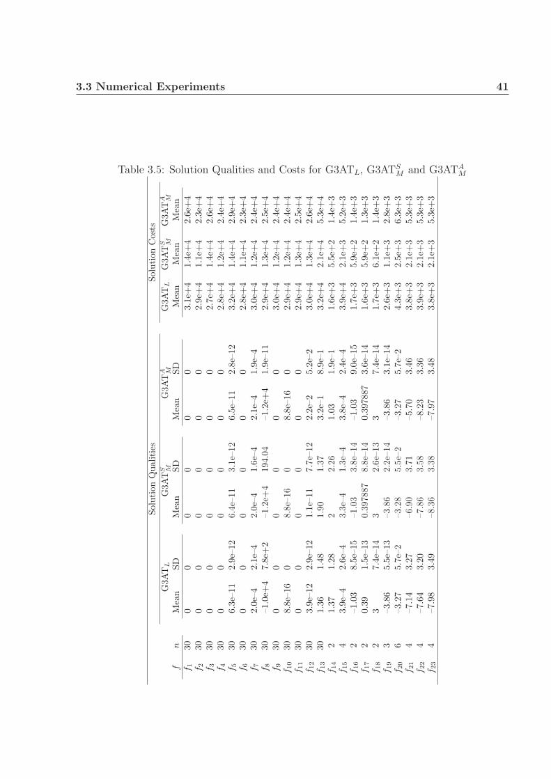
3.3 Numerical Experiments 41
Table 3.5: Solution Qualities and Costs for G3ATL, G3ATSM and G3ATA
M
Solu
tion
Qua
litie
sSo
luti
onC
osts
fn
f 130
f 230
f 330
f 430
f 530
f 630
f 730
f 830
f 930
f 10
30f 1
130
f 12
30f 1
330
f 14
2f 1
54
f 16
2f 1
72
f 18
2f 1
93
f 20
6f 2
14
f 22
4f 2
34
G3A
TL
G3A
TS M
G3A
TA M
Mea
nSD
00
00
00
00
6.3e
–11
2.9e
–12
00
2.0e
–42.
1e–4
–1.0
e+4
7.8e
+2
00
8.8e
–16
00
03.
9e–1
22.
9e–1
21.
361.
481.
371.
283.
9e–4
2.6e
–4–1
.03
8.5e
–15
0.39
1.5e
–13
37.
4e–1
4–3
.86
5.5e
–13
–3.2
75.
7e–2
–7.1
43.
27–7
.64
3.20
–7.9
83.
49
Mea
nSD
00
00
00
00
6.4e
–11
3.1e
–12
00
2.0e
–41.
6e–4
–1.2
e+4
194.
040
08.
8e–1
60
00
1.1e
–11
7.7e
–12
1.90
1.37
22.
263.
3e–4
1.3e
–4–1
.03
3.8e
–14
0.39
7887
8.8e
–14
32.
6e–1
3–3
.86
2.2e
–14
–3.2
85.
5e–2
–6.9
03.
71–7
.86
3.58
–8.3
63.
38
Mea
nSD
00
00
00
00
6.5e
–11
2.8e
–12
00
2.1e
–41.
9e–4
–1.2
e+4
1.9e
–11
00
8.8e
–16
00
02.
2e–2
5.2e
–23.
2e–1
8.9e
–11.
031.
9e–1
3.8e
–42.
4e–4
–1.0
39.
0e–1
50.
3978
873.
6e–1
43
7.4e
–14
–3.8
63.
1e–1
4–3
.27
5.7e
–2–5
.70
3.46
–8.2
33.
36–7
.97
3.48
G3A
TL
G3A
TS M
G3A
TA M
Mea
nM
ean
Mea
n3.
1e+
41.
4e+
42.
6e+
42.
9e+
41.
1e+
42.
3e+
42.
7e+
41.
4e+
42.
6e+
42.
8e+
41.
2e+
42.
4e+
43.
2e+
41.
4e+
42.
9e+
42.
8e+
41.
1e+
42.
3e+
43.
0e+
41.
2e+
42.
4e+
42.
9e+
41.
3e+
42.
5e+
43.
0e+
41.
2e+
42.
4e+
42.
9e+
41.
2e+
42.
4e+
42.
9e+
41.
3e+
42.
5e+
43.
0e+
41.
3e+
42.
6e+
43.
2e+
42.
1e+
45.
3e+
41.
6e+
35.
5e+
21.
4e+
33.
9e+
42.
1e+
35.
2e+
31.
7e+
35.
9e+
21.
4e+
31.
6e+
35.
9e+
21.
3e+
31.
7e+
36.
1e+
21.
4e+
32.
6e+
31.
1e+
32.
8e+
34.
3e+
32.
5e+
36.
3e+
33.
8e+
32.
1e+
35.
3e+
33.
9e+
32.
1e+
35.
3e+
33.
8e+
32.
1e+
35.
3e+
3

42Genetic Algorithms Combined with Accelerated Mutation and Automatic
Termination
Table 3.6: Rank-sum Test for G3ATL and G3ATSM Results
Compared Methods Solution Qualities Solution CostsMethod 1 Method 2
G3ATL G3ATSM
G3ATL G3ATAM
G3ATSM G3ATA
M
R+ R− p-value Best Method144 132 0.9822 –140 136 1 –
167.5 108.5 0.9556 –
R+ R− p-value Best Method
0 276 0.0052 G3ATSM
57.5 218.5 0.0861 –276 0 0.0121 G3ATS
M
1 2 3 4 5 6 7 8 9 10 11 12 13 14 15 16 17 18 19 20 21 22 23−500
0
500
1000
1500
2000
2500
3000
Test Functions
Err
ors
Solution Errors
G3AT
L
G3ATSM
G3ATAM
1 2 3 4 5 6 7 8 9 10 11 12 13 14 15 16 17 18 19 20 21 22 230
1
2
3
4
5
6x 10
4
Test Functions
Fin
tnes
s E
valu
atio
ns
Solution Costs
G3AT
L
G3ATMS
G3ATMS
Figure 3.10: Results of Table 3.5.

3.4 Numerical Comparisons 43
Table 3.7: GM within a Simple GAFunction f8 f18 f20
GM Zeros Percentage 80.50% 82.22% 84.97%
1 2 3 4 5 6 7 8 9 10 11 12 13 14 15 16 17 18 19 200
500
1000
1500
2000
2500
3000
3500
4000
Runs
Fun
ctio
n E
valu
atio
ns
f18
G3ATMS
GA
1 2 3 4 5 6 7 8 9 10 11 12 13 14 15 16 17 18 19 200
2000
4000
6000
8000
10000
12000
14000
16000
Runs
Fun
ctio
n E
valu
atio
ns
f20
G3ATMS
GA
Figure 3.11: Results of 20 independent runs of G3ATSM and GA (with GM).
In order to analyze the impact that the introduction of GM has on a simple GA, GM
has been implemented within a canonical GA, without any additional operator (such as
mutagenesis). GM is initialized as in G3ATSM and is updated after generating the offspring
in each generation. Three test functions are used in this experiment as shown in Table 3.7.
For each test function, GA is terminated at the same generation number as in G3ATSM . At
the end of each run, the percentage of zero entries to all entries of GM are reported in Table
3.7. Even if the maximum number of generations used for terminating GA is doubled, these
percentages will not be significantly improved. This indicates that there are many partitions
of the search space that are not well explored with a simple GA and this may explain
the low success rates of GA, as shown later in Table 3.22. Moreover, this highlights the
significant role of the proposed mutation and mutagenesis operations that enforce G3ATSM
to explore the search space widely. In addition, results of 20 independent runs of G3ATSM
and GA are shown in Figure 3.11. For test functions f18 and f20, Figure 3.11 shows that
G3ATSM tends to save function evaluation costs. For test function f8, GA could not achieve
the objective function value obtained by G3ATSM within a computational budget of 100,000
function evaluations although it is almost 8 times the budget needed by G3ATSM .
3.4 Numerical Comparisons
The best version G3ATSM was compared with two other advanced GAs; the Orthogonal GA
(OGA/Q) (Leung and Wang, 2001), and the Hybrid Taguchi-Genetic Algorithm (HTGA)
(Tsai et al., 2004), as well as four other EAs; the Covariance Matrix Adaptation Evolution

44Genetic Algorithms Combined with Accelerated Mutation and Automatic
Termination
Strategy (CMA-ES) (Hansen and Kern, 2004; Hansen, 2006) and its global restart version
G-CMA-ES (Hansen et al., 2005a,b), the Real-Coded Memetic Algorithms (RCMA) (Lozano
et al., 2005), and the Restart q-Gaussian mutation Evolution Strategy (RqGES) (Tinos and
Yang, 2011). More details about these methods are stated below.
• Orthogonal GA with Quantization (OGA/Q) (Leung and Wang, 2001). It is a modified
version of a classical GA (CGA). OGA/Q is identical to CGA, except that it uses the
orthogonal design to generate the initial population and the offspring of the crossover
operator.
• Hybrid Taguchi-Genetic Algorithm (HTGA) (Tsai et al., 2004). HTGA combines the
traditional GA with the Taguchi method (Taguchi et al., 2000), which can exploit
promising offspring. Taguchi method is incorporated in the crossover operations to
select better genes to achieve crossover and enhance the genetic algorithm.
• Covariance Matrix Adaptation Evolution Strategy (CMA-ES) (Hansen and Kern, 2004;
Hansen, 2006). CMA-ES is an evolution strategy method that invokes an adaptation
process of the covariance matrix. The main advantage of using the covariance matrix
is to detect a second order model of the underlying objective function similar to the
approximation of the inverse Hessian matrix in the Quasi-Newton method in classical
optimization.
• Global restart Covariance Matrix Adaptation Evolution Strategy (G-CMA-ES) (Hansen
et al., 2005a,b). G-CMA-ES is a modified version of CMA-ES in which premature
convergence can be detected and then a restart strategy is launched by doubling the
population size on each restart. By increasing the population size, the search char-
acteristic becomes more global after each restart, which empowers the operation of
the CMA-ES on multi-modal functions. G-CMA-ES is the winner of the CEC 2005
optimization competition.
• Real-Coded Memetic Algorithms (RCMA) (Lozano et al., 2005). RCMA uses the in-
dividual fitness to decide when local search is applied and how much effort should
be made. The individuals of the population are divided into three different categories
based on their fitness values. Local search parameters are set according to the category
to which an individual belongs.
• Restart q-Gaussian mutation Evolution Strategy (RqGES) (Tinos and Yang, 2011).
RqGES uses a Gaussian mutation with self-adaptation of the shape of the mutation
distribution in evolutionary algorithms. The shape of the Gaussian mutation distribu-
tion is controlled by a real parameter q which is encoded in the chromosomes in order
to evolve during the evolutionary process.

3.4 Numerical Comparisons 45
Table 3.8: Solution Qualities for G3ATSM , HTGA and OGA/Q
Solution Qualities
f n
f1 30f2 30f3 30f4 30f5 100f7 30f8 30f9 30f10 30f11 30f12 30f13 30f24 100f25 100
G3ATSM HTGA OGA/Q
Mean SD0 00 00 00 02.2e–010 02.0e–4 1.6e–4–12155.34 194.040 08.8e–16 00 01.1e–11 7.7e–121.90 1.37–93.31 1.14–72.68 1.46
Mean SD0 00 00 00 00.7 01.0e–3 0–12569.46 00 00 00 01.0e–6 01.0e–4 0–92.83 0–78.3 0
Mean SD0 00 00 00 00.752 0.1146.3e–3 4.1e–4–12569.45 6.4e–40 04.4e–16 4.0e–170 06.0e–6 1.2e–61.9e–4 2.6e–5–92.83 2.6e–2–78.3 6.3e–3
The results of these compared methods are taken from their original papers. These
results were obtained from 50 runs. It is worthwhile to mention that the reported results for
G3ATSM are based on achieving a full GM termination.
3.4.1 G3ATSM against Other GAs Using Classical Test Functions
The comparison results for G3ATSM , HTGA and OGA/Q are reported in Tables 3.8 and 3.9
along with Figure 3.12. They contain the mean and the standard deviation (SD) of the best
solutions obtained for each function and the average number of function evaluations. All the
compared methods (G3ATSM , HTGA and OGA/Q) are neutral on 7 out of 14 problems in
terms of solution qualities. Moreover, we observe that G3ATSM outperforms the other two
methods on 4 problems, while HTGA and OGA/Q outperform G3ATSM on 3 problems in
terms of solution qualities. On the other hand, G3ATSM consistently outperforms the other
two methods in terms of solution costs. Actually, G3ATSM is cheaper than HTGA and much
cheaper than OGA/Q. The results of the rank-sum test shown in Table 3.10 confirm these
conclusions. Specifically, there is no significant difference between each pair of G3ATSM ,
HTGA and OGA/Q in terms of solution qualities. However, G3ATSM is significantly cheaper
than the other two methods in terms of solution costs with a p-value of
p = 1− [(1− 0.0307) · (1− 7.0× 10⁻⁶)] = 0.0307067851.

46Genetic Algorithms Combined with Accelerated Mutation and Automatic
Termination
Table 3.9: Solution Costs for G3ATSM , HTGA and OGA/Q
Solution Costsf n
f1 30f2 30f3 30f4 30f5 100f7 30f8 30f9 30f10 30f11 30f12 30f13 30f24 100f25 100
G3ATSM HTGA OGA/Q
1.41e+4 1.43e+4 1.13e+51.17e+4 1.28e+4 1.13e+51.40e+4 1.54e+4 1.13e+51.23e+4 1.46e+4 1.13e+53.88e+4 3.93e+4 1.68e+51.22e+4 1.28e+4 1.13e+51.35e+4 1.11e+5 3.02e+51.20e+4 1.51e+4 2.25e+51.20e+4 1.41e+4 1.12e+51.36e+4 1.61e+4 1.34e+51.38e+4 3.43e+4 1.35e+52.05e+4 2.06e+4 1.34e+54.49e+4 2.19e+5 3.03e+55.07e+4 2.05e+5 2.46e+5
Table 3.10: Rank-sum Test for G3ATSM , HTGA and OGA/Q Results
Compared Methods Solution Qualities Solution CostsMethod 1 Method 2
G3ATSM HTGA
G3ATSM OGA/Q
HTGA OGA/Q
R+ R− p-value Best Method56.5 48.5 0.9421 –56.5 48.5 0.9809 –18 87 0.7899 –
R+ R− p-value Best Method
105 0 0.0307 G3ATSM
105 0 7.0× 10⁻⁶ G3ATSM
105 0 3.5× 10⁻⁶ HTGA
1 2 3 4 5 7 8 9 10 11 12 13 24 25
10−20
10−15
10−10
10−5
100
105
Test Functions
Err
ors
Solution Errors
G3ATMS
HTGAOGA/Q
1 2 3 4 5 7 8 9 10 11 12 13 24 250
0.5
1
1.5
2
2.5
3
3.5x 10
5
Test Functions
Fun
ctio
n E
valu
atio
ns
Soultion Costs
G3ATMS
HTGAOGA/Q
Figure 3.12: Results of Tables 3.8 and 3.9.

3.4 Numerical Comparisons 47
1 2 3 4 5 6 7 8 9 10 11 12 13 14 15 16 17 18 19 20 21 22 23
10−20
10−15
10−10
10−5
100
105
Test Functions
Err
ors
Solution Errors
G3AT
MS
CMA−ES
1 2 3 4 5 6 7 8 9 10 11 12 13 14 15 16 17 18 19 20 21 22 2310
2
103
104
105
106
Test Functions
Fun
ctio
n E
valu
atio
ns
Soultion Costs
G3ATMS
CMA−ES
Figure 3.13: Results of Table 3.11.
3.4.2 G3ATSM against CMA-ES and Its Variants
One of the most promising and efficient modifications of evolution strategies (ESs) is CMA-
ES (Hansen and Kern, 2004; Hansen, 2006). In the following, we discuss the results of
G3ATSM against CMA-ES and its global restart version G-CMA-ES using the figures shown
in Tables 3.11 and 3.13. The results reported in Table 3.11 contain the success rate of a trial
judged by means of the condition
|f ∗ − f | < ε, (3.4.1)
where f ∗ refers to the known exact global minimum value, f refers to the best function value
obtained by the algorithm, and ε is a small positive number, which is set equal to 10−3 in
our experiments. Condition (3.4.1) is only used to check the success of the result obtained
from each run. The results of Table 3.11 are summarized in Figure 3.13.
The percentages between parentheses in Table 3.11 represent the success rate under
condition (3.4.1). To make fair comparisons between G3ATSM and CMA-ES, the latter
is terminated after reaching the same number of function evaluations needed by G3ATSM .
Therefore, both of them have the same solution costs. In terms of solution qualities or
success rates, CMA-ES did not outperform G3ATSM except for function f13. Actually, the
rank-sum test results shown in Table 3.12 indicate that there is no significant difference
between G3ATSM and CMA-ES in terms of solution qualities. However, G3ATS
M obtained
significantly better success rates compared to those obtained by CMA-ES.
The results of CMA-ES can be improved by using its restart version G-CMA-ES (Hansen
et al., 2005a,b). Table 3.13 shows the results of G-CMA-ES with two restarts for the func-
tions for which CMA-ES fails at reaching comparable success rates against G3ATSM . Table
3.14 presents the rank-sum test figures for the results presented in Table 3.13. From these
statistical results, we can observe that there is no significant difference between G3ATSM and

48Genetic Algorithms Combined with Accelerated Mutation and Automatic
Termination
Table 3.11: Solution Qualities for G3ATSM and CMA-ES
f n
f1 30f2 30f3 30f4 30f5 30f6 30f7 30f8 30f9 30f10 30f11 30f12 30f13 30f14 2f15 4f16 2f17 2f18 2f19 3f20 6f21 4f22 4f23 4
G3ATSM CMA-ES
Mean SD0(100%) 00(100%) 00(100%) 00(100%) 06.40e–11(100%) 3.1e–120(100%) 02.00e–4(100%) 1.6e–4–1.2e+4(0%) 194.040(100%) 08.80e–16(100%) 00(100%) 01.10e–11(100%) 7.7e–121.90(4%) 1.372(74%) 2.263.30e–4(100%) 1.3e–4–1.03(100%) 3.8e–140.397887(100%) 8.8e–143(100%) 2.6e–13–3.86(100%) 2.2e–14–3.28(70%) 6.0e–2–6.90 (56%) 3.71–7.86(66%) 3.58–8.36(70%) 3.38
Mean SD4.43e–21 (100%) 1.17e–211.51e–09 (100%) 3.45e–096.66e–08 (100%) 1.63e–073.79e–06 (100%) 4.46e–061.85e+01 (0%) 1.77e+002.80e–01 (80%) 6.14e–012.14e–01 (0%) 6.62e–02–7.61e+03 (0%) 8.56e+014.86e+01 (0%) 1.36e+015.04e–11 (100%) 8.44e–121.08e–03 (88%) 3.11e–031.24e–02 (88%) 3.44e–024.39e–04 (96%) 2.20e–031.46e+01 (0%) 1.89e–134.98e–03 (48%) 1.78e–02–1.03e+00 (100%) 3.51e–163.98e–01 (100%) 1.69e–146.24e+00 (88%) 8.95e+00–3.86e+00 (100%) 7.08e–16–3.27e+00 (60%) 5.96e–02–4.65e+00 (16%) 2.69e+00–4.80e+00 (20%) 3.01e+00–4.67e+00 (28%) 3.74e+00
Table 3.12: Rank-sum Test for G3ATSM and CMA-ES Results in Table 3.11
Comparing Criterion Compared MethodsSolution Qualities G3ATS
M CMA-ESSuccess Rates G3ATS
M CMA-ES
R+ R− p-value Best Method259.5 16.5 0.1131 –233.5 42.5 0.0233 G3ATS
M
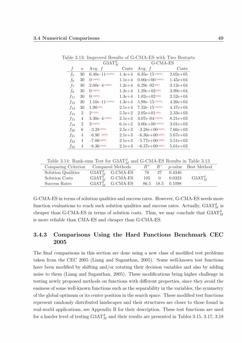
3.4 Numerical Comparisons 49
Table 3.13: Improved Results of G-CMA-ES with Two RestartsG3ATS
M G-CMA-ESf n Avg. f Costs Avg. f Costsf5 30 6.40e–11(100%) 1.4e+4 6.35e–15(100%) 2.02e+05f6 30 0(100%) 1.1e+4 0.00e+00(100%) 1.45e+04f7 30 2.00e–4(100%) 1.2e+4 6.29e–02(0%) 3.12e+04f9 30 0(100%) 1.2e+4 1.29e+02(0%) 3.99e+04f11 30 0(100%) 1.3e+4 1.02e+02(0%) 2.52e+04f12 30 1.10e–11(100%) 1.3e+4 5.98e–15(100%) 4.26e+04f13 30 1.90(4%) 2.1e+4 7.32e–15(100%) 4.47e+04f14 2 2(74%) 5.5e+2 2.05e+01(0%) 2.33e+03f15 4 3.30e–4(100%) 2.1e+3 3.07e–04(100%) 8.21e+03f18 2 3(100%) 6.1e+2 3.00e+00(100%) 3.01e+03f20 6 –3.28(70%) 2.5e+3 –3.28e+00(64%) 7.66e+03f21 4 –6.90 (56%) 2.1e+3 –6.36e+00(48%) 5.67e+03f22 4 –7.86(66%) 2.1e+3 –5.77e+00(39%) 5.51e+03f22 4 –8.36(70%) 2.1e+3 –6.37e+00(48%) 5.61e+03
Table 3.14: Rank-sum Test for G3ATSM and G-CMA-ES Results in Table 3.13
Comparing Criterion Compared MethodsSolution Qualities G3ATS
M G-CMA-ESSolution Costs G3ATS
M G-CMA-ESSuccess Rates G3ATS
M G-CMA-ES
R+ R− p-value Best Method78 27 0.4340 –105 0 0.0323 G3ATS
M
86.5 18.5 0.1098 –
G-CMA-ES in terms of solution qualities and success rates. However, G-CMA-ES needs more
function evaluations to reach such solution qualities and success rates. Actually, G3ATSM is
cheaper than G-CMA-ES in terms of solution costs. Thus, we may conclude that G3ATSM
is more reliable than CMA-ES and cheaper than G-CMA-ES.
3.4.3 Comparisons Using the Hard Functions Benchmark CEC2005
The final comparisons in this section are done using a new class of modified test problems
taken from the CEC 2005 (Liang and Suganthan, 2005). Some well-known test functions
have been modified by shifting and/or rotating their decision variables and also by adding
noise to them (Liang and Suganthan, 2005). These modifications bring higher challenge in
testing newly proposed methods on functions with different properties, since they avoid the
easiness of some well-known functions such as the separability in the variables, the symmetry
of the global optimum or its center position in the search space. These modified test functions
represent randomly distributed landscapes and their structures are closer to those found in
real-world applications, see Appendix B for their description. These test functions are used
for a harder level of testing G3ATSM and their results are presented in Tables 3.15, 3.17, 3.18

50Genetic Algorithms Combined with Accelerated Mutation and Automatic
Termination
1 2 3 4 5 6 7 8 9 10 1110
−14
10−12
10−10
10−8
10−6
10−4
10−2
100
102
104
106
Test Functions
Err
ors
Solution Errors
G3ATMS
RCMA
1 2 3 4 5 6 7 8 9 10 110
1
2
3
4
5
6
7
8
9
10
11x 10
4
Test FunctionsF
unct
ion
Eva
luat
ions
Soultion Costs
G3ATMS
RCMA
Figure 3.14: Results of Table 3.15 for test functions h1–h11 with n = 10.
1 2 3 4 5 6 7 8 9 10 1110
−14
10−12
10−10
10−8
10−6
10−4
10−2
100
102
104
106
Test Functions
Err
ors
Solution Errors
G3ATMS
RCMA
1 2 3 4 5 6 7 8 9 10 110
0.5
1
1.5
2
2.5
3
3.5x 10
5
Test Functions
Fun
ctio
n E
valu
atio
ns
Soultion Costs
G3ATMS
RCMA
Figure 3.15: Results of Table 3.15 for test functions h1–h11 with n = 30.
and 3.19.
The results of Real-Coded Memetic Algorithm (RCMA) (Lozano et al., 2005) are also
presented in Table 3.15 to discuss the efficiency of the proposed method. The convergence
performance of G3ATSM and that of RCMA are almost the same. However, the accelerated
automatic termination enables G3ATSM to achieve cheaper function evaluations than RCMA.
The statistical results of the rank-sum test shown in Table 3.16 confirm these conclusions.
Other comparisons are presented here to test the performance of G3ATSM against G-
CMA-ES, the winner of CEC 2005 competition, and against the recently proposed RqGES
method. The results of these comparisons are reported in Tables 3.17, 3.18 and 3.19. They
are summarized in Figures 3.16, 3.17 and 3.18, and statistically analyzed in Tables 3.20 and
3.21. All these results yield the same conclusions as above. Namely, G3ATSM could obtain
competitive solution qualities with cheaper costs. Actually, G3ATSM requires significantly

3.4 Numerical Comparisons 51
Table 3.15: Results for Shifted and Shifted-Rotated Functions
Solu
tion
Qua
litie
s(E
rror
s)So
luti
onC
osts
Func
tion
No.
nh
110
h2
10h
310
h4
10h
510
h6
10h
710
h8
10h
910
h10
10h
11
10h
130
h2
30h
330
h4
30h
530
h6
30h
730
h8
30h
930
h10
30h
11
30
G3A
TS M
RC
MA
Mea
nSD
6.59
4e–1
32.
990e
–13
1.57
3e–1
21.
448e
–12
3.16
6e–9
1.58
2e–8
3.83
5e+
26.
401e
+2
7.14
3e+
11.
070e
+2
9.56
8e–1
1.73
8e+
07.
120e
–25.
928e
–22.
957e
–51.
015e
–47.
960e
–22.
755e
–21.
588e
+1
6.83
6e+
05.
843e
+0
1.16
9e+
08.
242e
–13
4.56
4e–1
38.
516e
–10
4.56
4e–1
01.
604e
+0
2.72
7e+
03.
333e
+4
1.02
6e+
46.
277e
+3
1.73
4e+
33.
987e
–11.
261e
+0
1.04
0e–2
1.00
0e–3
4.79
1e–6
1.13
3e–5
4.77
6e+
02.
428e
+0
1.26
9e+
22.
221e
+1
2.62
1e+
11.
7243
e+0
Mea
nSD
9.86
9e–9
6.61
7e–2
59.
936e
–90
4.77
1e+
46.
496e
+3
1.99
7e–8
2.52
6e–9
2.12
4e–2
1.87
9e–2
1.49
0e+
05.
402e
–21.
971e
–12.
066e
–22.
019e
+1
1.37
6e–2
4.37
8e–1
9.87
6e–2
5.64
3e+
03.
618e
–14.
557e
+0
5.24
3e–1
9.36
4e–9
1.89
9e–1
08.
717e
–67.
474e
–78.
775e
+5
5.81
0e+
43.
966e
+1
8.55
4e+
02.
183e
+3
7.83
1e+
14.
955e
+1
1.93
3e+
11.
329e
–21.
272e
–32.
071e
+1
3.76
6e–2
6.80
6e–1
1.21
4e–1
9.05
8e+
14.
892e
+0
3.11
4e+
11.
525e
+0
Ave
rage
no.
offu
ncti
onev
alua
tion
sG
3AT
S M
8926
8968
1125
283
7985
4392
1787
9182
7386
8188
6482
7024
770
2852
342
183
2219
023
249
5033
123
908
2214
322
510
2265
522
186
RC
MA
100,
000
100,
000
100,
000
100,
000
100,
000
100,
000
100,
000
100,
000
100,
000
100,
000
100,
000
300,
000
300,
000
300,
000
300,
000
300,
000
300,
000
300,
000
300,
000
300,
000
300,
000
300,
000
Table 3.16: Rank-sum Test for G3ATSM and RCMA Results in Table 3.15
Solution Qualities Solution Costsn Compared Methods R+ R− p-value Best Method R+ R− p-value Best Method
10 G3ATSM RCMA 34 32 0.7427 – 66 0 2.5377× 10⁻⁵ G3ATS
M30 G3ATS
M RCMA 36 30 0.4307 – 66 0 2.5377× 10⁻⁵ G3ATSM
All G3ATSM RCMA 133 120 0.4047 – 253 0 8.4593× 10⁻⁹ G3ATS
M

52Genetic Algorithms Combined with Accelerated Mutation and Automatic
Termination
Table 3.17: Results for the Hard Functions h1–h17 with n = 10G3ATS
M G-CMA-ES RqGESFunction Error Cost Error Cost Error Cost
h1 1.60e–12 8611 5.20e–09 10,000 3.77e–08 100,000h2 2.95e–09 9,170 4.70e–09 10,000 3.76e–08 100,000h3 7.53e–04 10,026 5.60e–09 10,000 1.55e+05 100,000h4 1.21e+03 14,152 5.02e–09 10,000 6.29e–08 100,000h5 1.92e+02 9,878 6.58e–09 10,000 1.05e–04 100,000h6 6.38e–01 10,058 1.17e+01 10,000 8.23e+02 100,000h7 1.57e–01 9,508 2.27e–03 10,000 1.40e–03 100,000h8 2.00e+01 9,270 2.05e+01 10,000 2.04e+01 100,000h9 5.93e–13 8,469 6.21e+00 10,000 1.49e+00 100,000h10 1.81e+01 8,563 7.16e+00 10,000 1.72e+00 100,000h11 5.09e+00 8,868 4.42e+00 10,000 1.69e–01 100,000h12 3.00e+02 9,070 2.98e+03 10,000 1.05e+03 100,000h13 4.42e–01 8,968 9.71e–01 10,000 1.09e+00 100,000h14 3.52e+00 10,509 3.91e+00 10,000 2.91e+00 100,000h15 1.23e+02 8,630 2.99e+02 10,000 1.98e+02 100,000h16 1.28e+02 8,943 1.11e+02 10,000 9.37e+01 100,000h17 1.60e+02 14,184 1.95e+02 10,000 9.59e+01 100,000
reduced solution costs compared to G-CMA-ES and RqGES with a p-value of
p = 1− [(1− 1.0101× 10−9) · (1− 1.9276× 10⁻¹⁸)] = 1.010100003639991× 10⁻⁹.
3.5 G3ATSM against GA MATLAB Toolbox
In this section, the G3ATSM method is compared with GA MATLAB included in “MATLAB
Genetic Algorithm and Direct Search Toolbox”. The algorithm implemented in the GA
1 2 3 4 5 6 7 8 9 10 11 12 13 14 15 16 1710
−14
10−12
10−10
10−8
10−6
10−4
10−2
100
102
104
106
Test Function
Err
ors
Solution Errors
G3ATSM
G−CMA−ESRqGES
1 2 3 4 5 6 7 8 9 10 11 12 13 14 15 16 1710
3
104
105
Test Function
Fun
ctio
n E
valu
atio
ns
Solution Costs
G3ATSM
G−CMA−ESRqGES
Figure 3.16: Results of Table 3.17 for test functions h1–h17 with n = 10.

3.5 G3ATSM against GA MATLAB Toolbox 53
Table 3.18: Results for the Hard Functions h1–h17 with n = 30G3ATS
M G-CMA-ES RqGESFunction Error Cost Error Cost Error Cost
h1 6.96e–12 23,654 5.42e–09 100,000 1.54e–06 300,000h2 8.24e–08 27,896 6.22e–09 100,000 1.74e–06 300,000h3 3.36e+00 34,865 5.55e–09 100,000 9.43e+05 300,000h4 3.81e+04 43,251 1.27e+04 100,000 4.58e–01 300,000h5 6.12e+03 30,388 1.08e–07 100,000 2.31e+03 300,000h6 7.07e–01 36,288 4.78e–01 100,000 1.75e+03 300,000h7 1.06e–02 28,291 5.31e–09 100,000 2.69e–03 300,000h8 2.00e+01 28,021 2.07e+01 100,000 2.10e+01 300,000h9 4.74e+00 23,132 6.89e+00 100,000 9.74e+00 300,000h10 1.14e+02 23,415 6.96e+00 100,000 9.24e+00 300,000h11 2.32e+01 24,268 9.10e+00 100,000 3.60e+00 300,000h12 1.60e+03 27,076 5.95e+04 100,000 8.90e+03 300,000h13 1.98e+00 29,069 2.89e+00 100,000 3.26e+00 300,000h14 1.28e+01 38,136 1.35e+01 100,000 1.24e+01 300,000h15 3.33e+02 24,534 2.25e+02 100,000 3.37e+02 300,000h16 1.92e+02 25,108 5.34e+01 100,000 1.77e+02 300,000h17 2.79e+02 43,321 2.92e+02 100,000 1.04e+02 300,000
Table 3.19: Results for the Hard Functions h1–h17 with n = 50G3ATS
M G-CMA-ES RqGESFunction Error Cost Error Cost Error Cost
h1 3.52e–11 37,116 5.87e–9 100,000 7.21e–03 500,000h2 2.24e–07 47,262 7.86e–9 100,000 2.16e–03 500,000h3 8.63e+00 65,952 4.84e+01 100,000 1.13e+06 500,000h4 1.03e+05 73,537 6.16e+05 100,000 7.85e+02 500,000h5 1.45e+04 49,725 1.21e+03 100,000 6.38e+03 500,000h6 1.11e+02 66,398 3.74e+01 100,000 6.74e+02 500,000h7 7.10e–03 47,020 7.22e–9 100,000 1.43e–02 500,000h8 2.00e+01 44,754 2.11e+01 100,000 2.11e+01 500,000h9 1.94e+01 36,233 2.19e+01 100,000 5.89e+01 500,000h10 2.83e+02 36,685 2.61e+01 100,000 2.40e+01 500,000h11 4.47e+01 38,166 2.12e+01 100,000 1.28e+01 500,000h12 6.29e+03 45,919 4.84e+05 100,000 4.31e+04 500,000h13 4.28e+00 55,248 5.48e+00 100,000 5.63e+00 500,000h14 2.24e+01 66,316 2.30e+01 100,000 2.18e+01 500,000h15 3.17e+02 39,465 2.50e+02 100,000 3.53e+02 500,000h16 2.43e+02 42,570 6.50e+01 100,000 4.99e+01 500,000h17 3.83e+02 73,528 2.36e+02 100,000 3.20e+01 500,000

54Genetic Algorithms Combined with Accelerated Mutation and Automatic
Termination
Table 3.20: Rank-sum Test for Solution Qualities Reported in Tables 3.17–3.19n Compared Methods R+ R− p-value Best Method10 G3ATS
M G-CMA-ES 85 68 0.8363 –G3ATS
M RqGES 78 75 0.9725 –G-CMA-ES RqGES 49 104 0.5816 –
30 G3ATSM G-CMA-ES 54 99 0.4084 –
G3ATSM RqGES 74 79 0.9177 –
G-CMA-ES RqGES 95 58 0.2416 –50 G3ATS
M G-CMA-ES 65 88 0.8633 –G3ATS
M RqGES 79 74 0.7566 –G-CMA-ES RqGES 79.5 73.5 0.7176 –
All G3ATSM G-CMA-ES 584 742 0.4028 –
G3ATSM RqGES 666 660 0.8122 –
G-CMA-ES RqGES 667.5 667.5 0.1907 –
Table 3.21: Rank-sum Test for Solution Costs Reported in Tables 3.17–3.19n Compared Methods R+ R− p-value Best Method10 G3ATS
M G-CMA-ES 153 0 0.0118 G3ATSM
G3ATSM RqGES 153 0 1.1467× 10⁻⁷ G3ATS
M
G-CMA-ES RqGES 153 0 1.0363× 10⁻⁸ G-CMA-ES30 G3ATS
M G-CMA-ES 153 0 1.1467× 10⁻⁷ G3ATSM
G3ATSM RqGES 153 0 1.1467× 10⁻⁷ G3ATS
M
G-CMA-ES RqGES 153 0 1.0363× 10⁻⁸ G-CMA-ES50 G3ATS
M G-CMA-ES 153 0 1.1467× 10⁻⁷ G3ATSM
G3ATSM RqGES 153 0 1.1467× 10⁻⁷ G3ATS
M
G-CMA-ES RqGES 153 0 1.0363× 10⁻⁸ G-CMA-ESAll G3ATS
M G-CMA-ES 1285.5 40.5 1.0101× 10⁻⁹ G3ATSM
G3ATSM RqGES 1326 0 1.9276× 10⁻¹⁸ G3ATS
M
G-CMA-ES RqGES 1326 0 3.0707× 10⁻¹³ G-CMA-ES
1 2 3 4 5 6 7 8 9 10 11 12 13 14 15 16 1710
−12
10−10
10−8
10−6
10−4
10−2
100
102
104
106
Test Function
Err
ors
Solution Errors
G3ATSM
G−CMA−ESRqGES
1 2 3 4 5 6 7 8 9 10 11 12 13 14 15 16 1710
4
105
106
Test Function
Fun
ctio
n E
valu
atio
ns
Solution Costs
G3ATSM
G−CMA−ESRqGES
Figure 3.17: Results of Table 3.18 for test functions h1–h17 with n = 30.

3.5 G3ATSM against GA MATLAB Toolbox 55
1 2 3 4 5 6 7 8 9 10 11 12 13 14 15 16 1710
−12
10−10
10−8
10−6
10−4
10−2
100
102
104
106
108
Test Function
Err
ors
Solution Errors
G3ATSM
G−CMA−ESRqGES
1 2 3 4 5 6 7 8 9 10 11 12 13 14 15 16 1710
4
105
106
Test Function
Fun
ctio
n E
valu
atio
ns
Solution Costs
G3ATSM
G−CMA−ESRqGES
Figure 3.18: Results of Table 3.19 for test functions h1–h17 with n = 50.
1 2 3 4 5 6 7 8 9 10 11 12 13 14 15 16 17 18 19 20 21 22 23
10−20
10−15
10−10
10−5
100
105
Test Functions
Err
ors
Solution Errors
G3ATMS
GA
1 2 3 4 5 6 7 8 9 10 11 12 13 14 15 16 17 18 19 20 21 22 230
10
20
30
40
50
60
70
80
90
100
Test Functions
Suc
cess
Rat
es (
%)
Success Rates
G3ATMS
GA
Figure 3.19: Results of Table 3.22.
MATLAB toolbox is a basic GA. We compared it with our best version of G3AT using
the same number of function evaluations and the same GA parameters. To refine the best
solution found by GA MATLAB, a built-in hybrid Nelder-Mead method is used to keep an
equal level of search strategies between GA MATLAB and G3ATSM . The success rate of a
trial is judged by means of condition (3.4.1).
From the results shown in Table 3.22 and summarized in Figure 3.19, we can conclude
that using the mutagenesis operation can help a simple GA (such as the one found in the
GA MATLAB toolbox) to achieve better results with faster convergence. This is confirmed
by the statistical results presented in Table 3.23. Indeed, the difference between the two
methods in terms of both solution qualities and success rates is statistically significant.
Actually, it seems that GA MATLAB was sometimes trapped in local minima even for
some easy functions like f18. As shown in Figure 3.20, the global minimum of f18 lies
in a widespread valley. Therefore, it is not difficult for a search method with an efficient

56Genetic Algorithms Combined with Accelerated Mutation and Automatic
Termination
Table 3.22: Solution Qualities for G3ATSM and GA MATLAB
f n
f1 30f2 30f3 30f4 30f5 30f6 30f7 30f8 30f9 30f10 30f11 30f12 30f13 30f14 2f15 4f16 2f17 2f18 2f19 3f20 6f21 4f22 4f23 4
G3ATSM GA MATLAB
Mean SD0(100%) 00(100%) 00(100%) 00(100%) 0
6.4e–11(100%) 3.1e–120(100%) 0
2.0e–4(100%) 1.6e–4–1.2e+4(0%) 194.04
0(100%) 08.8e–16(100%) 0
0(100%) 01.1e–11(100%) 7.7e–12
1.90(4%) 1.372(74%) 2.26
3.3e–4(100%) 1.3e–4–1.03(100%) 3.8e–14
0.397887(100%) 8.8e–143(100%) 2.6e–13
–3.86(100%) 2.2e–14–3.28(70%) 6.0e–2
–6.90 (56%) 3.71–7.86(66%) 3.58–8.36(70%) 3.38
Mean SD1.1e–11(100%) 4.9e–11
8.88(0%) 1.781.8e+4(2%) 5.1e+3
21.62(0%) 11.081.8e+3(0%) 2.4e+3769.34(0%) 225.71
0.27(0%) 8.9e–2–9.3e+3(0%) 7.1e+3
38.90(0%) 10.585.64(0%) 0.66
1.2e–11(100%) 1.1e–116.55(2%) 2.645.62(2%) 2.236.04(24%) 5.41
2.3e–3(42%) 1.8e–3–1.03(100%) 2.3e–14
0.397887(100%) 3.1e–136.48(90%) 21.06
–3.86(100%) 1.5e–14–3.26(50%) 6.0e–2–5.19(26%) 3.13–6.13(38%) 3.44–5.99(36%) 3.53
Table 3.23: Rank-sum Test for G3ATSM and GA MATLAB Results
Comparing Compared MethodsCriteria Method 1 Method 2 R+ R− p-value Best Method
Solution Qualities G3ATSM GA MATLAB 273 3 0.0185 G3ATS
M
Success Rates G3ATSM GA MATLAB 265.5 10.5 1.5663×10⁻⁴ G3ATS
M

3.6 Conclusion 57
Figure 3.20: Goldstein & Price Function f18.
exploration process to reach the global minimum. However, GA MATLAB failed to reach
the global minimum in 10% of the trials.
3.6 Conclusion
In this chapter, we have introduced a new GA that is equipped with the GM, mutagenesis
and a final intensification process. We have shown that G3AT is robust and able to reach
global minima or at least be very close to them in many test problems. The use of GM
effectively assists the algorithm to achieve wide exploration and deep exploitation before
stopping the search. This indicates that our main objective, which is to equip evolution-
ary algorithms with automatic accelerated termination criteria, has largely been fulfilled.
Moreover, the proposed intensification schemes based on mutagenesis of GM and Best Child
Inspiration have proved to be more efficient in our experiments than local search based on
the Nelder-Mead method. Among the three versions of G3AT, G3ATSM is the one showing
the best general performance. The comparison results indicate that G3ATSM undoubtedly
outperforms the GA MATLAB toolbox and is much cheaper than some advanced versions of
GAs as well as some other EAs. Moreover, even though the proposed method uses a classical
type of crossover, it is very competitive with some state-of-art methods. Therefore, the newly
added elements in the proposed method contribute in achieving good performance. Finally,
we may conclude that using mutagenesis could improve the solution quality and using the
GM to determine termination criteria could reduce the amount of function evaluations.

58Genetic Algorithms Combined with Accelerated Mutation and Automatic
Termination

Chapter 4
Genetic Algorithm with AutomaticTermination and Search SpaceRotation
In the last two decades, numerous EAs have been developed for solving optimization prob-
lems. However, only a few works have focused on the question of the termination criteria.
Indeed, EAs still need termination criteria prespecified by the user. In this chapter, we
develop another GA with automatic termination and acceleration elements which allow the
search to end without resort to predefined conditions. We call this algorithm Genetic Al-
gorithm with Automatic Termination and Search Space Rotation, abbreviated as GATR.
This algorithm utilizes the GM to equip the search process with a self-check in order to
judge how much exploration has been performed, while maintaining the population diver-
sity. The algorithm also implements the mutagenesis operation to achieve more efficient and
faster exploration and exploitation processes. Moreover, GATR improves the performance
of G3AT by fully exploiting the structure of the GM by calling a novel search space de-
composition mechanism combined with a search space rotation procedure. As a result, the
search operates strictly within two-dimensional subspaces irrespective of the dimension of
the original problem. The computational experiments and comparisons with some state-
of-the-art EAs demonstrate the effectiveness of the automatic termination criteria and the
space decomposition mechanism of GATR.
4.1 Introduction
We propose in this chapter an improved version of G3AT presented in Chapter 3. G3AT is
originally a GA with new directing strategies. The key elements of G3AT are the GM, the
mutagenesis operator and a final intensification process. The GM is a matrix constructed
to represent subranges of the possible values of each variable and consequently reflects the
60 Genetic Algorithm with Automatic Termination and Search Space Rotation
distribution of the genes over the search range. Its role is to assist the exploration process in
two different ways. First, GM can provide the search with new diverse solutions by applying
the mutagenesis operator. Mutagenesis operator is a new type of mutation that works in
combination with GM. It alters some individuals in order to accelerate the exploration and
exploitation processes by guiding the search specifically towards unexplored areas. Also, GM
is the key component to let G3AT know how far the exploration process has been performed
in order to determine an adequate termination instant. By definition, however, although
numerical experiments lead to positive results, the GM is a two-dimensional structure and
there is no evidence that it is able to represent the distribution of individuals in the multi-
dimensional search space accurately, especially in high-dimensional, multi-modal and highly
epistatic problems. We thus provide in this chapter a response to those considerations, while
attempting to improve the performance of the G3AT algorithm. We keep focused, however,
on the main objective of this study, that is, on the automatic termination. We would like
to stress out that our main objective is not to outperform existing results, although we will
show that the method proposed in this chapter is competitive.
The response is a rotation-based version of the G3AT method, designated as GATR,
which stands for Genetic Algorithm with Automatic Termination and Search Space Rotation.
The main new elements are the Space Decomposition (SD) and the Space Rotation (SR). SD
and SR work in combination in order to create a two-dimensional environment for the GM
irrespective of the original dimension of the problem to be solved. In this environment, the
GM goes through a series of rotations which allow the search to avoid premature convergence
and termination due to specificities of the problems. As a hybrid GA, GATR first emphasizes
on exploring the whole search space using the GM. Afterward, the exploitation process is
invoked through a local search method in order to refine the best candidates obtained so far.
GATR thus behaves like a “Memetic Algorithm” (Moscato, 1999; Le et al., 2009) in order
to achieve faster convergence (Ong and Keane, 2004; Ong et al., 2006; Jakob, 2010; Kramer,
2010).
The performance of the algorithm is evaluated in 10, 30 and 50 dimensions on the set
of 25 test problems of the CEC 2005 real-parameter optimization contest (Suganthan et al.,
2005) and compared against a number of existing algorithms such as G3AT, a Real-Coded
Memetic Algorithm (RCMA) (Lozano et al., 2005), a version of the Evolution Strategy with
Covariance Matrix Adaptation method (which is a well-known state-of-the-art method for
adaptive mutation) that is combined with a restart strategy (L-CMA-ES) (Hansen and Kern,
2004; Hansen, 2006) as well as the recent Non-Revisiting Genetic Algorithm with Parameter-
less Adaptive Mutation (NrGA) (Yuen and Chow, 2009), a Differential Evolution method
using an adaptive local search (DEahcSPX) (Noman and Iba, 2008) and the winner of the
CEC 2005 competition, the Restart CMA Evolution Strategy With Increasing Population
Size (G-CMA-ES) (Hansen et al., 2005b).

4.2 GATR Mechanisms 61
The rest of the chapter is organized as follows. Section 4.2 provides a review of the
mechanisms implemented in GATR. It includes the GM and the mutagenesis operator as
well as the new concepts developed to reinforce the GM model. The SD and SR are also
described in this section. The effects of the introduction of the new mechanisms are discussed
in Section 4.3. In Section 4.4, components and the formal algorithm of GATR are detailed.
In Section 4.5, the methodology adopted for the numerical experiments is explained and
results in dimensions 10, 30 and 50 are presented with the benchmark functions from CEC
2005. A comparative study against other methods from the literature is also conducted. A
summary with conclusions is provided in Section 4.6.
4.2 GATR Mechanisms
GATR uses the Simple GM and mutagenesis operator described in Section 2.4. However, in
GATR, the SD and SR mechanisms create solely two-dimensional environments that affect
the GM. For that reason, the definition of the GM undergoes a slight adaptation, described
in this section. Also, new concepts that reinforce the GM model are presented here. G3AT
and GATR are methods that aims to determine a stopping point without knowledge about
the problem. However, we also want GATR to be a method that not only possesses a proper
stopping judgement but also exhibits more accurate and versatile performance than G3AT
against a wider class of problems.
4.2.1 Gene Matrix and Termination
GATR adopts the real-coding representation of individuals. Hence in the search space,
every individual x consists of n variables or genes. The range of each gene is divided into m
subranges in order to check the diversity of the gene values. In GATR, GM is initialized as
a 2×m zero matrix in which each entry of the i-th row refers to a subrange of the i-th gene.
Indeed, in GATR, GM deals solely with two-dimensional subspaces, although the problem
being optimized can be of any dimension n ≥ 2. While the search is processing, the entries of
GM are updated if new values for genes are generated within the corresponding subranges.
Those entries are granted with a non-null value. Specifically, during the search, the value of
each gene is considered in order to extract the number associated with the subrange where
the considered gene is located, say v ∈ {1, . . . ,m}. Let xi be the representation of the i-th
gene, i = 1, . . . , n. Once a gene gets a value corresponding to a non-explored subrange, GM
is updated by flipping a zero into a one in the corresponding (i, v) entry. Let us note that,
with this mechanism, GM is not sensitive to the number of genes lying inside each subrange.
After having a GM full, i.e., with no zero entry, the search judges that an advanced
exploration process has been achieved and can be stopped. In this way, the principal use

62 Genetic Algorithm with Automatic Termination and Search Space Rotation
Figure 4.1: Diagonal distribution of individuals before and after rotation and the associatedGM.
of GM is to equip the search process with a practical termination tool. Other versions
of GM, sensitive to the number of genes within each subrange, have been investigated.
However, our comparative study has revealed that the zero-one GM mechanism presented
here (and implemented in GATR) yields the best performances in terms of number of function
evaluations versus solution quality.
4.2.2 High-dimensional Search Space
By definition, GM has a two-dimensional structure, i.e., a matrix of indicator variables for
subranges in each dimension of the search space. Consequently, it may face some difficulties
in representing the distribution of individuals in a high-dimensional search space. Basically,
for m subranges and n dimensions, we can count mn hyperrectangles in the search space.
However the GM can become complete with less than m × n points. Therefore, there is a
possibility of having a misguided termination of the exploration process, as depicted in a
simple example in Figure 3.2(a), where the GM is already full although the search space
is far from being entirely covered. The crossover operation can overcome this drawback as
shown in Figure 3.2(b). As a matter of fact, numerical simulations show that GM explores
the search space widely. However, although it is easy to comprehend in two dimensions,
it is difficult to admit whether such mechanism can perform a sufficient exploration of the
search space when the dimension of the problem increases, which is one of the reasons why
we introduce the SR and SD mechanisms.
4.2.3 Space Rotation
Those considerations on GM prompt us to develop the space rotation mechanism. As de-
picted in Figure 4.1(a), a particular distribution of the individuals may lead to premature
completion of GM. Indeed in this case, it is clear that the entire search space has not been
fully covered. In Figure 4.1(b), after applying to the search space a clockwise 45 degrees
rotation, the same distribution of the explored areas is seen by GM from a different angle.

4.2 GATR Mechanisms 63
Figure 4.2: NR rotations of the search space by angle α and the associated GM.
Recomputing the GM then reveals unexplored regions (i.e., the matrix is not complete any
more). Thus in order to escape from premature termination of the search, the idea is to
“rotate” the search space and attach to the resulting spaces a GM that do not necessarily
have the same configuration as the original one at a given instant.
Let us consider the optimization problem (1.1.1) defined in Section 1.1. The search
domain D can be seen as an n-dimensional rectangle in Rn. The edges of this rectangle
are given by the lower bounds li and upper bounds ui of the variables xi with li ≤ xi ≤ ui
(i = 1, ..., n).
The rotation of the rectangle is depicted in Figure 4.2. Rotation is defined by the rotation
angle α, which is a divisor of 360, as well as the number of rotations, NR = 360/α. To each
rotation is associated a GM, namely GMl, l = 0, . . . , NR − 1. They are independently fed
by their respective rotated spaces.
During the search process, SR applies the rotation operator, named Rotα[x], to each
individual x using angle α such that x′ = Rotα[x], where x′ represents the rotated individual.
Then the original objective function can be recomputed by f(x) = f(Rot−1α [x′]). Formal
description of SR is given in Procedure 4.2.1, where xi represents the i-th gene of each
individual x within the population X, and X ′ is the population in the rotated subspace
associated with its GM that will be denoted as GM′. Each population is of size µ.
Procedure 4.2.1. Rotation(X ′, GM ′)
1. Set values of α. Set Rotα :=
[cos α − sin αsin α cos α
].
2. For each individual x in X, let x′i := (Rotα[x])i, i = 1, ..., n.3. Update GM ′ using all individuals x′, and return.
The SR mechanism can be compared to a previous work by Schwefel that first appeared
in (Schwefel, 1974) and also later in (Beyer and Schwefel, 2002). In that work, Schwefel
introduces the idea of correlated mutation based on rotation of the solution space by using

64 Genetic Algorithm with Automatic Termination and Search Space Rotation
a rotation matrix for a variant of EA, namely, the Evolution Strategies (ES) (Rechenberg,
1965; Beyer and Schwefel, 2002). One of the peculiarities of ES is that individuals not only
comprise the decision variables but also a set of strategy parameters. Among them, we can
find those of the mutation operator. Hence, the decision variables along with the strategy
parameters evolve simultaneously during the evolution process. However, in essence this
strategy is different from SR. Indeed, the rotation matrix introduced by Schwefel aims at
improving the mutation operation by controlling the area of the search space where are
generated individuals. SR, on the other hand, do not aim at composing new individuals but
rather ensuring that GM has explored a widespread area of the search space and detecting
unexplored regions.
4.2.4 Space Decomposition
GM and SR are by nature two-dimensional mechanisms. For problems in higher dimensions,
we invoke the space decomposition mechanism. Its role is to transform a high-dimensional
search space of a problem into several two-dimensional subspaces. In order to do so, before
the search process, SD selects two variables, say xa and xb, among {x1, x2, . . . , xn}, which
will be referred to as the current “active variables”. During the generation process, only xa
and xb are directly treated as the variables to be manipulated. The other variables, referred
to as “passive variables”, momentarily hold their values fixed (i.e., they will not participate
in the improvement for a moment). The upper and lower bounds of xa and xb are used to
define the edges of the rectangle that will be considered by SR. At the end of the search,
all genes of the best individual found (both active and passive variables) are given a chance
to be improved in an intensification phase. The resulting candidate (individual) is referred
to as xelite. At this point, we end the search using the GM information, but obviously the
obtained xelite does not announce the end of the entire process since we have only considered
a portion of variables. Thus, if “enough” genes have not participated yet in the search as
active variables, the current ones are set as passives and two other genes are selected as new
actives. The search is then resumed, as what we will call a new “era”. It is important to
understand that the entire process will end when enough active variables have participated
in their own eras. However, it is the role of the GM to terminate adequately each era.
The efficiency of the whole algorithm is thus under the influence of the performance of the
automatic termination. At the beginning of each era, the whole population is randomly
generated. However, once the passive variables are designated, the values of all individuals’
passive variables (or genes) are transformed in such a way that their values are aligned with
those of the previously obtained xelite.
4.3 Effects of the GATR Mechanisms 65
4.3 Effects of the GATR Mechanisms
Although GATR is used as an optimization tool, its parameters cannot be set to be optimal
for all problems at the same time. Since GATR is not a self-adaptive method, in order
to observe the guideline proposed by the CEC 2005, we have decided to run preliminary
experiments on the test bed and observe which parameter values would give the best results
on a large set of test functions. In particular, we here discuss the effects of the introduction
of each component of GATR and how the parameter values have been determined and used
in this work.
4.3.1 Number of Subranges of the GM
The parameter m regulates the size of the sub-regions and its suitable value appears to
be very problem dependent. The number of function evaluations, abbreviated as Feval, is
directly proportional to m in any dimension, but the success rates, referred to as SRate
and defined later in Subsection 4.5.1, have unpredictable behaviors. For our numerical
experiments, the convergence speed has been given more importance, since the Feval with
m varying from 50 to 300 can dramatically increase, while SRate keeps fluctuating and does
not necessarily increase significantly. It is thus favorable to keep m as small as possible. In
our experiments, m = 100 was the value demonstrating the most satisfactory results on a
large set of functions in terms of SRate, with moderate Feval.
4.3.2 Effect of the Space Decomposition
Here we discuss the effects of the introduction of SD into G3AT. To do so, a variant of G3AT,
referred to as SD-G3AT, has been implemented. This variant employs SD with G3AT, but
using a single GM without rotations, and only one intensification phase during the final era,
as in G3AT. SD-G3AT is compared against G3AT in terms of SRate and Feval in 10 and 30
dimensions.
As shown in Figure 4.3(a) and 4.4(a) for functions f1–f15 in 10 and 30 dimensions, re-
spectively, the use of SD (through SD-G3AT), i.e., using solely n = 2 during the search,
tends to slightly decrease the required Feval before termination (except function f2 in 30
dimensions, for which Feval is slightly higher). Performance in terms of SRate in 10 dimen-
sions, as shown in Figure 4.3(b), is advantageous for SD-G3AT. Functions that could be
solved by G3AT were also solved by SD-G3AT. Moreover, SD-G3AT could perform better
for functions f3 and f6, and could also solve functions f7 and f9. Figure 4.4(b) depicts the
results achieved in 30 dimensions. We can observe that SRate stays around the same order.
Functions f1 and f2 could be solved by both variants. We also note that function f7 could
not be solved by G3AT, but could be handled (with a small SRate) by SD-G3AT.

66 Genetic Algorithm with Automatic Termination and Search Space Rotation
(a) (b)
Figure 4.3: Comparison of Feval and SRate for G3AT vs SD-G3AT on functions f1–f15 in10 dimensions.
(a) (b)
Figure 4.4: Comparison of Feval and SRate for G3AT vs SD-G3AT on functions f1–f15 in30 dimensions.
Thus, in terms of Feval and SRate, the introduction of SD could slightly accelerate the
convergence of the algorithm, and obtain equivalent or better SRate.
4.3.3 Number of Space Rotations
In GATR, the role of the rotations is to lower the possibility of premature termination at a
non-optimal solution, which is caused by insufficient exploration of the search space due to
the structure of the GM. We have tested GATR with different numbers of space rotations
NR ranging between 0 and 4, where NR = 0 means no rotation. Thus only the impact of SD
was measured, as in Subsection 4.3.2. We could observe that Feval is directly proportional
to NR. It can be estimated that the introduction of one rotation in 30 dimensions increases
the Feval by around 5.4% on average, while in 10 dimensions it increases the Feval by around
10%. Also high NR tends to slow down the algorithm. Starting with no rotation, after 3
rotations, the functions that could not be solved before came with positive results. Thus,

4.3 Effects of the GATR Mechanisms 67
to keep an acceptable convergence speed, we have decided to adopt NR = 3 as the default
value in our numerical experiments.
4.3.4 Combination List
The CL is a list that keeps track of the pairs of variables that are designated to participate
during the eras. Let us consider the pair {xa, xb}. Obviously xa and xb should not be
identical. One of the easiest and most intuitive way to construct the CL is to select randomly
xa and xb from the set of all possible variables {x1, x2, . . . , xn} with the only condition that
xa is different from xb. However, experiments show that selecting the active variables in a
sequential manner (i.e., starting with x1 and x2, then x3 and x4, etc.) could provide equal
or better results for all functions. Although there is no theoretical proof to support this
finding, we decided to adopt the “sequential” way of creating the CL (as opposed to the
random construction) in GATR.
Now, we are concerned about the length of the CL (CL length) (i.e., the number of
eras), which has a direct impact on the convergence speed of the search. According to our
preliminary experiments, it is without surprise that the cost in Feval increases proportionally
with the length of the CL. Intuitively, one can expect better SRate with a longer CL, since
more eras would be allowed to refine a solution. However, the results show that SRate
increases slowly or fluctuates with CL length for many functions. Moreover, a length of
5 and 15 in 10 and 30 dimensions, respectively, provided in general good performance in
terms of SRate on a large set of problems. Increasing those values may improve slightly
the SRate, but the Feval will considerably increase at the same time. According to those
results, in GATR, CL length has been set equal to round(n/2), where the operation round
rounds towards the nearest integer. This value aims at good SRate with acceptable Feval.
Note that setting CL length = round(n/2) guarantees that each variable is given a chance
to participate in the search as an active variable at least once.
4.3.5 Intensification
Intensification is the process whose purpose is to refine the elite solution obtained at the
end of an era. In GATR as well, intensification calls a local search process based on the
Kelley’s modification (Kelley, 1999) of the Nelder-Mead (NM) method (Nelder and Mead,
1965). The use of systematic intensification at the end of each era, however, can be expen-
sive in terms of Feval. In GATR, intensification is therefore sparingly called by specific eras
since it yields positive effects when called at intermediate stages of the search. We should
remark, however, that the final refinement by intensification at the end of the search is most
important to achieve higher accuracy. Indeed, GM combined with the SD and SR can be
seen as the components that will explore the search space widely in order to find promising

68 Genetic Algorithm with Automatic Termination and Search Space Rotation
individuals. Those individuals will be given a chance to improve further through an ex-
ploitation phase handled by intensification. The numbers designating the eras that will go
through an intensification step are stored in the intensification list (IL). Preliminary exper-
iments, using the terminology introduced in Subsection 4.5.1 concerning the test functions
and methodology, show that the best results are obtained when the first and last eras are
subject to intensification. Various patterns to select the remaining eras have been studied.
However, no significative differences can be observed when compared to a random selection
of the intermediate intensified eras. The total number of eras that go through intensification
(i.e., the length of IL) has also been studied. Intensification calls a local search method at
the end of an era. Consequently, it relatively requires a considerable amount of additional
computational resources. As a matter of fact, experiments show that a longer IL consider-
ably increase Feval. However, SRate does not necessarily increase for all functions. Thus,
in order to keep a good balance between exploration and exploitation, the length of IL in
GATR has been set equal to n/5.
It should also be noted that although GATR relies on intensification when it comes to
the exploitation phase, intensification alone cannot reach the results obtained by GATR.
Indeed, experiments on some functions, such as f9 for instance, revealed that the success
rate for that function could reach 36% using GATR over the 25 trials. On the same function,
the use of intensification only and using random starting points led to a success rate of 0%.
From this simple experiment, we may observe that intensification has an important part to
play in GATR. However, if used alone, the results are not satisfactory compared to GATR.
It is thus in combination with GATR that superior results could be achieved.
4.3.6 Termination
In order to estimate whether the GMs are able to provide the search with a correct ter-
mination point, the automatic termination has been compared for each function with the
same run in the same conditions, as described in Subsection 4.5.1, but with an artificially
maintained higher number of generations and only one final intensification occurring during
the last era. For function f10 in 10 dimensions for instance, Figure 4.5(a) represents the evo-
lution of the error with Feval using GATR and only one final intensification, referred to as
Short-GATR. We can observe that around 5,100 Fevals were required to reach an error level
of around 1.6. The dotted vertical line represents the instant at which the algorithm decided
to stop and launch the final intensification phase. Intensification could improve the results
by reducing the error from roughly 1.8 to 1.6. Figure 4.5(b) depicts the evolution of the error
over Feval obtained by a modified version of GATR, called Long-GATR, whose termination
instant was artificially delayed. To do so, CL length has been set equal to 15 instead of 5
(i.e., round(n/2)) in the original setting. More eras were thus allowed to explore the search

4.4 GATR Operators and Formal Algorithm 69
(a) (b)
Figure 4.5: Comparison of termination instant after intensification (vertical dotted line) forfunction f10 using Short-GATR (a) and Long-GATR (b).
space. Also, CP was set equal to 100% instead of 90% in order to obtain longer eras and
let the search refine the obtained solutions further. In Long-GATR, around 16,500 Fevals
were necessary before termination, which is slightly more than 3 times the short version. We
can see that after around 4,000 Fevals, which is the instant at which Short-GATR decided
to stop, the improvement in terms of error begins to stagnate at around 1.8. After 10,000
function evaluations, the error improvement is still not significative. Finally, intensification
could reduce the error from around 1.75 to 1.5. This experiment reveals that letting the
search run after the original termination instant does not necessarily improve the best solu-
tion obtained, considering the substantial amount of additional Feval required to improve a
solution further.
4.4 GATR Operators and Formal Algorithm
Before stating the formal algorithm of GATR, basic components that compose a GA and
that are used by GATR are briefly described in this section.
4.4.1 GA Operators
The parent selection mechanism implemented in GATR is based on the linear ranking se-
lection mechanism (Baker, 1985; Hedar and Fukushima, 2003). This mechanism ranks the
initial population P according to the fitness function value of each individual. From P , an
intermediate population P ′ is produced by copying repeatedly individuals based on their
fitness ranking until P ′ becomes full. Note that an already chosen individual can be se-
lected more than once. In GATR, since n = 2 during the search, the crossover operation is
straightforward. The procedure consists in swapping the active variables of two parents p1

70 Genetic Algorithm with Automatic Termination and Search Space Rotation
and p2, and create two children c1 and c2. The mutation operator is designed to take advan-
tage of the information contained in the GM. Indeed, existing zeros from GM are randomly
selected, say in the position (i, j), and a randomly chosen individual from the intermediate
pool IPM has its variable xi modified by a new value lying inside the j-th partition of its
range. For each individual in the intermediate population P ′ and for each gene, a random
number from the interval (0, 1) is associated. If the associated number is less than a prespec-
ified mutation probability πm, then the individual is copied to the intermediate pool IPM .
The number of times the associated numbers are less than the mutation probability πm is
counted, and let numm denote this number. Afterward the mutation operation ensures that
the total number numm of genes to be mutated does not exceed the number of zeros in the
GM, denoted numzeros. Otherwise the number of genes is reduced to numzeros. The formal
procedure for mutation is analogous to Procedure 2.4.1, where m represents the number of
each gene’s subranges. Parents and children then compete together for survival, making
GATR a steady-state GA.
Procedure 4.4.1. Mutation(x,GM)
1. If GM is full, then return; otherwise, go to Step 2.2. Choose a zero-position (i, j) in GM randomly.3. Update x by setting xi = li + (j − r)ui−li
m, where r is a random number from
(0, 1), and li, ui are the lower and upper bounds of the variable xi, respectively.4. Update GM and return.
4.4.2 GATR Formal Algorithm
The search process in GATR is repeated several times, with different active variables taking
part in distinct eras. Each search can be considered to be a G3AT run for a two-dimensional
problem, taking advantage of GM and SR to terminate adequately. Preliminaries consist in
SD whose role is to transform an n-dimensional search space into several two-dimensional
subspaces. During an era, GATR starts by generating an initial population of size µ and
dimension n. Two variables, xa and xb, are chosen as active variables. They will participate
in the current era’s evolution, while the other genes have their values replicated from xelite’s
respective gene values. In the very first era, however, each gene of xelite is pre-initialized
as xelitei := (ui+li
2), where li and ui are the lower and upper bounds of gene xi, respectively.
For any n-dimensional problem, CL length eras are carried out with distinct pairs of active
variables, and the values of passive genes remain unchanged during each era.
As a GA based method, GATR evaluates the population members, and then generates
offsprings by applying parent selection, crossover and mutation operations. The role of SR
is to manipulate the two-dimensional space in which the active variables are evolved by
executing NR rotations of angle α. NR distinct GMs are updated, each corresponding to

4.4 GATR Operators and Formal Algorithm 71
one of the NR rotated subspaces. Mutagenesis is invoked until the GM completion ratio
CP , which may be set as different from 1, is reached. An era terminates when all NR
GMs reach CP . Eventually, it is guaranteed that the GMs will reach CP since mutagenesis
makes sure that new individuals are generated within unvisited areas. It is worthwhile
to mention that the main role of GM and SR is to guide the search towards unexplored
regions, while exploration by itself is conducted by the crossover and mutagenesis operations.
The termination of the algorithm is thus guaranteed. Finally, an era ends with a final
intensification phase that uses a local search method in order to refine the best solution
found so far. Let us emphasize that each era consecutively improves the current best solution
xelite by using the active variables. However, intensification improves all genes, actives and
passives. The solution xelite is then used in the starting point for the next era, where a
different couple of active variables is selected and the remaining ones become passive. When
all the pairs of variables in CL have actively participated in some eras, GATR terminates
with the last refined solution. A formal description of GATR is given below.
Algorithm 4.4.2. GATR Algorithm
1. Initialization. Set values of m, µ, µw, NR, α, CP , and (li, ui) for i =1, . . . , n. Set the crossover and mutation probabilities πc ∈ (0, 1) and πm ∈(0, 1), respectively. Set the Intensification List IL as described in Subsection4.3.5. Set the Combination List CL := {x1, x2, . . . , xn}. If the number ofelements in CL is odd, add a randomly chosen element from {x1, x2, . . . , xn}.Set the generation counter t := 1. Compute xelite by xelite
i := ui+li2
for i =1, . . . , n.
2. Set all variables to be passive. Select xa and xb from CL. Update CL byCL := CL\{xa, xb} and designate xa and xb as active variables.2.1. Generate an initial population P0 of size µ and update each individualxk in P0 so that xk
i := xelitei for i ∈ {1, . . . , n}\{a, b}.
2.2. Initialize Gene Matrices GMl, l = 1, ..., NR, as 2 × m zero matrices,where GMl corresponds to the l-th space rotation.
3. Parent Selection. Evaluate the fitness function F for all individuals in Pt.Select an intermediate population of parents P ′
t from the current populationPt. Let the initial parent pool SPt and children pool SCt be empty.
4. Crossover. Associate a random number from (0, 1) with each individual inP ′
t and add this individual to the parent pool SPt if the associated number isless than πc. Repeat the following Steps 4.1 and 4.2 until all chosen parentsfrom SPt are mated:4.1. Choose two parents p1 and p2 from SPt. Mate p1 and p2 by swappingtheir active variables to create children c1 and c2.4.2. Update the children pool SCt by SCt := SCt ∪ {c1, c2} and update SPt bySPt := SPt \ {p1, p2}.
5. Mutation. Associate a random number from (0, 1) with each gene in eachindividual in P ′
t . Let numm be the number of genes whose associated number

72 Genetic Algorithm with Automatic Termination and Search Space Rotation
is less than πm, and let numzeros be the number of zero elements in GM. Ifnumm ≥ numzeros, then set numm := numzeros. Mutate numm individualsamong those which have an associated number less than πm by applying Pro-cedure 4.4.1. Add the mutated individual to the children pool SCt. UpdateGMl, l = 1, ..., NR with SR by applying Procedure 4.2.1.
6. If all GMs have reached the completion ratio CP , go to Step 9. Otherwise goto Step 7.
7. Survivor Selection. Evaluate the fitness function for all generated childrenSCt, and choose the µ best individuals in Pt ∪ SCt for the next generationPt+1.
8. Mutagenesis. Apply Procedure 2.4.1 to alter the µw worst individuals inPt+1, set t := t+1, update GMl, l = 1, ..., NR with SR by applying Procedure4.2.1, and go to Step 3.
9. Intensification. If the current era is in IL, then go to Step 9.1. Otherwisego to Step 9.2.9.1. Apply a local search method starting from the best solution obtained inthe previous search stage using all variables, and go to Step 9.2.9.2. Let xelite be the best solution obtained so far. If CL 6= ∅, go to Step 2.Otherwise, terminate with xelite.
4.5 Numerical Results
Numerical experiments were carried out to evaluate the performance of GATR. Before pre-
senting the results, we describe the methodology adopted to conduct the numerical study of
GATR.
4.5.1 Methodology
The numerical study is based on a test bed of 25 standard test functions from the special
session on real-parameter optimization in the IEEE Congress on Evolutionary Computations,
CEC 2005 (Suganthan et al., 2005). The set was carefully built based on classic benchmark
functions in an attempt to cover a diverse set of problem properties. The first 5 functions
are unimodal functions while the 20 other functions are multimodal, with functions f13 to
f25 being hybrid composition functions. The mathematical form of the 25 test problems can
be found in (Suganthan et al., 2005).
Before proceeding to the description of the test settings and results, some remarks should
be stated in order to emphasize the particularity of the proposed GATR method. This
is to clarify the dissimilarities in the way we present and compare the data with other
methods, which does not exactly follow the evaluation guideline suggested in CEC 2005.
When conducting numerical experiments, the CEC 2005 guideline recommends the use of

4.5 Numerical Results 73
Table 4.1: GATR Parameter SettingParameter Definition Valueµ Population size 30πc Crossover probability 0.6πm Mutation probability 0.1m No. of GM subranges 100µw No. of individuals used by mutagenesis 2NR Number of space rotations 3α Space rotation angle 45o
CP Completion ratio of GM 90%
common evaluation criteria such as the initialization scheme, the size of problems, a common
termination criterion, etc. The guideline in particular indicates that the search should be
stopped when reaching a pre-specified maximum number of function evaluations (10, 000×n)
or if the error in the function value becomes lower than a given threshold (10−8). Solution
quality is measured through the function error value given by (f(x) − f(x∗)), where f(x)
represents the best function value obtained by the algorithm and f(x∗) is the known exact
global minimum value. Also, when evaluating the amount of function evaluations needed,
the search is stopped as soon as a fixed accuracy level is achieved. It is clear that GATR
cannot fully comply with those termination criteria, since the point here is to let the search
terminate automatically. Consequently, the results of the numerical experiments are not
reported exactly as suggested in CEC 2005, but comparison is still possible and realistic, as
done in this section, where interesting findings are discussed.
Table 4.1 summarizes the GATR parameters with their assigned values. GATR was
programmed using MATLAB and the code for each test function was run 25 times in 10,
30 and 50 dimensions, in accordance with the guideline proposed in CEC 2005. Also, a run
is considered successful when the fixed accuracy level is achieved within the pre-specified
maximum number of function evaluations (before 100,000 Fevals in 10 dimensions, 300,000
Fevals in 30 dimensions and 500,000 Fevals in 50 dimensions). The success rate (SRate) is
defined as the number of successful runs divided by the total number of runs.
In this study, the Wilcoxon matched-pairs signed-ranks non-parametric test is used for
directly comparing the results of two methods. This test, as described in (Garcıa et al.,
2009), does not assume that the data are sampled from a normal distribution. It assumes
however that the data are symmetrically distributed around the median. We employ the
Wilcoxon non-parametric test because, for the methods that follow the framework suggested
by the CEC 2005, the authors report their achieved average results using the same conditions
for each algorithm and test problem. In particular, we consider in this work the function
error values obtained by each method.

74 Genetic Algorithm with Automatic Termination and Search Space Rotation
4.5.2 Discussion from the Benchmark Results
The 25 test functions of the CEC 2005 can be classified according to their characteristics.
Hence, we will discuss here the performance of GATR by taking into account the nature of
the functions. Results are available in Table 4.2 for GATR, where the mean error values are
reported for each functions as well the SRate, in parentheses, when not null. To begin with,
the first five functions are unimodal functions and the others are multimodal. Functions f1
and f2 are relatively easy to solve, in 10, 30 and 50 dimensions. The increase in dimension-
ality did not affect substantially the performance of the algorithm in terms of mean error
value. Function f3 is the shifted rotated high conditioned elliptic function and the optima
could be found only in 10 dimensions. Function f4 is similar to f2 but shifted with noise.
The addition of noise seems to have affected the performance. Function f6 could be solved
in all dimensions with decent success rates, due to the local search capability of GATR
through intensification. Function f7 is a shifted rotated version of Griewank’s function and
does not have predefined bounds. It was easy to solve even in high dimensions. Function f8
has a “needle in a haystack” profile and is thus very challenging to solve for most methods.
GATR got stuck at the same mean error value order in all dimensions. Functions f9 and
f10 are shifted and rotated shifted versions of the Rastrigin function, respectively, and f11
is also a shifted rotated function. The global optimum was missed in all runs for f10 and
f11. Function f12 is Schwefel’s problem and it could be solved in 10 dimensions. Function
f13 and f14 are expanded functions and could not be solved. Functions f15–f25 are hybrid
composition functions based on basic functions. In particular, comparing functions f21 and
f23 that have the same error order, we see that the algorithm did not seem affected when
discontinuity is introduced. In general, functions f15–f25 are designed to be very hard to
solve for any algorithm. Except f15 in 10 dimensions with low success rate, GATR as well
could not locate a global optimum for them under the requirements set by the CEC 2005
guideline.
4.5.3 Comparison with G3AT
With the intention of improving the G3AT method, the SD and SR mechanisms have been
developed and implemented within the GATR method. The aim of this section is to study
the impact of those new mechanisms within GATR against G3AT by comparing their results.
We first try to determine whether there is any significant difference between the two
methods using the Wilcoxon non-parametric test over the 25 benchmark functions of the
CEC 2005. Table 4.3 summarizes the results of the test in 10, 30 and 50 dimensions. The
signed ranked statistics are reported (R– for GATR and R+ for the compared method, here
G3AT) along with the indication of the significantly superior method at significance level 0.05
(for this test bed, the Wilcoxon critical value is equal to 89). The highest values of the test

4.5 Numerical Results 75
Table 4.2: Solution Qualities for GATR and G3AT with Significant Method in Bold andSRate in Parentheses
n=
10n
=30
n=
50
f f 1 f 2 f 3 f 4 f 5 f 6 f 7 f 8 f 9 f 10
f 11
f 12
f 13
f 14
f 15
f 16
f 17
f 18
f 19
f 20
f 21
f 22
f 23
f 24
f 25
GA
TR
G3A
TE
rror
Mea
n6.
84e–
13(1
00%
)2.
54e–
12(1
00%
)4.
73e–
12(1
00%
)1.
02e+
042.
28e+
023.
19e–
01(9
2%)
9.72
e–02
(12%
)2.
00e+
013.
98e–
13(8
8%)
4.63
e+01
1.12
e+01
9.48
e–12
(100
%)
4.92
e–01
4.01
e+00
3.79
e+01
(8%
)1.
46e+
022.
10e+
029.
00e+
029.
00e+
029.
00e+
024.
78e+
028.
38e+
027.
86e+
022.
91e+
024.
37e+
02
Err
orM
ean
6.21
e-13
(100
%)
2.23
e-12
(100
%)
1.20
e-03
(92%
)1.
54e+
031.
38e+
021.
50e+
00(7
2%)
2.25
e-01
2.00
e+01
2.83
e+00
1.83
e+01
7.59
e+00
3.09
e+02
(44%
)7.
34e-
013.
94e+
001.
48e+
021.
34e+
021.
89e+
028.
71e+
028.
84e+
028.
43e+
028.
86e+
028.
13e+
029.
99e+
022.
48e+
026.
54e+
02
GA
TR
G3A
TE
rror
Mea
n1.
12e-
12(1
00%
)1.
45e-
09(1
00%
)2.
11e+
021.
03e+
052.
29e+
035.
91e-
01(9
6%)
3.22
e-04
(100
%)
2.00
e+01
2.61
e-12
(36%
)5.
53e+
013.
10e+
013.
94e+
011.
73e+
001.
32e+
013.
67e+
027.
47e+
012.
77e+
029.
00e+
029.
00e+
029.
00e+
028.
82e+
025.
30e+
027.
40e+
022.
24e+
022.
22e+
02
Err
orM
ean
2.01
e-12
(100
%)
4.32
e-06
(100
%)
6.89
e+04
4.27
e+04
5.79
e+03
9.57
e+01
1.12
e-02
2.00
e+01
2.17
e+01
1.20
e+02
2.98
e+01
2.06
e+03
4.66
e+00
1.30
e+01
3.88
e+02
1.83
e+02
3.31
e+02
9.00
e+02
9.00
e+02
9.00
e+02
5.70
e+02
7.92
e+02
6.77
e+02
2.96
e+02
2.98
e+02
GA
TR
G3A
TE
rror
Mea
n6.
539e
-12
(100
%)
4.67
6e-0
8(1
00%
)6.
790e
+02
5.06
6e+
055.
473e
+03
2.71
8e+
00(5
6%)
1.10
2e-0
3(1
00%
)2.
000e
+01
4.97
5e+
001.
830e
+02
7.57
2e+
013.
535e
+03
3.09
2e+
002.
257e
+01
2.72
6e+
028.
559e
+01
3.52
8e+
029.
000e
+02
9.00
0e+
029.
000e
+02
7.43
9e+
025.
007e
+02
7.52
9e+
023.
189e
+02
3.23
0e+
02
Err
orM
ean
9.77
9e-1
2(1
00%
)3.
844e
-03
(96%
)1.
395e
+05
1.22
7e+
051.
614e
+04
4.67
7e+
028.
689e
-03
(60%
)2.
001e
+01
7.05
3e+
013.
161e
+02
5.70
4e+
019.
016e
+03
1.81
3e+
012.
254e
+01
4.47
0e+
022.
147e
+02
4.21
9e+
029.
000e
+02
9.00
0e+
029.
000e
+02
7.44
6e+
025.
144e
+02
7.52
2e+
028.
712e
+02
8.25
9e+
02

76 Genetic Algorithm with Automatic Termination and Search Space Rotation
Table 4.3: Wilcoxon’s Test for GATR against G3AT (at level 0.05)n GATR (R–) G3AT (R+) Significant Method103050
147236261
1788964
–GATRGATR
statistics represent the best results. From Table 4.3, we note that in dimension 10, GATR
and G3AT are not significantly different. In higher dimensions however, for dimensions 30
and 50, GATR significantly outperforms G3AT, the gap getting bigger as the dimension
increases. The introduction of the SD and SR mechanisms thus seems particularly effective
in higher dimensions.
Since both G3AT and GATR are under automatic termination, it is possible to empir-
ically compare their results using the framework proposed in CEC 2005 and get a better
insight of the performance of GATR on a function-level rather than on a method-level. We
support our findings by the paired Student’s t-test (Montgomery and Runger, 2003) using
the mean error as well as the error standard deviation (not reported). Table 4.2 reports the
results of G3AT and GATR in 10, 30 and 50 dimensions using the same test bed as for the
Wilcoxon’s test. The results of a significantly superior method at level 0.05 for each func-
tion are reported in bold font. The Feval, reported in Table 4.4, indicates that GATR is on
average around 1.4 times more expensive in terms of function evaluations in 10 dimensions.
In 30 and 50 dimensions, the computational cost in Feval approximately doubles on average.
The introduction of SD and SR mechanisms is however not the principal cause of the raise
of Feval. It is the increase of frequency of the local searches during the intensification phase,
which has a more predominant weight in the total Feval cost of GATR. In 10 dimensions,
t-tests indicate that GATR gives significantly better solutions than G3AT in terms of so-
lution quality on 9 functions, while G3AT is significantly better on 5 functions. The gap
gets bigger in 30 and 50 dimensions. In 30 dimensions, GATR performs significantly better
on 10 functions while G3AT performs better on 3 functions. In 50 dimensions, out of the
25 problems, G3AT achieves significantly better results for only 3 problems, while GATR
outperforms G3AT in 14 problems. Those improved results, especially in higher dimensions,
demonstrate the efficiency of the SD and SR mechanisms, especially when the problem com-
plexity increases. In addition, it is worth pointing out that the SD and SR mechanisms
themselves do not increase the running time of the algorithm. The additional running time
in GATR when compared to G3AT comes from the intensification steps. Roughly speaking,
the running time is proportional to Fevals in both GATR and G3AT. Experiments carried
out using a computer with 3 GHz Intel Core 2 Duo processor and 3 GB of RAM reveals
that for function f1 in 50 dimensions for instance, the measured CPU time was around 37
seconds for G3AT and 95 seconds for GATR.

4.5 Numerical Results 77
Table 4.4: Solution Costs for GATR and G3AT
n=
10n
=30
n=
50
f f 1 f 2 f 3 f 4 f 5 f 6 f 7 f 8 f 9 f 10
f 11
f 12
f 13
f 14
f 15
f 16
f 17
f 18
f 19
f 20
f 21
f 22
f 23
f 24
f 25
GA
TR
G3A
TFe
valM
ean
6.24
e+03
6.31
e+03
1.26
e+04
4.63
e+03
5.72
e+03
1.17
e+04
6.21
e+03
4.01
e+03
5.41
e+03
5.61
e+03
4.51
e+03
6.39
e+03
6.01
e+03
6.13
e+03
5.12
e+03
5.34
e+03
5.02
e+03
6.12
e+03
6.25
e+03
6.26
e+03
6.94
e+03
5.15
e+03
5.24
e+03
5.27
e+03
4.83
e+03
Feva
lM
ean
4.22
e+03
4.28
e+03
7.87
e+03
3.60
e+03
3.91
e+03
9.05
e+03
4.18
e+03
3.52
e+03
4.14
e+03
4.16
e+03
3.55
e+03
4.30
e+03
4.28
e+03
4.67
e+03
3.85
e+03
3.87
e+03
3.64
e+03
4.10
e+03
4.24
e+03
4.23
e+03
4.10
e+03
3.77
e+03
3.72
e+03
4.65
e+03
3.67
e+03
GA
TR
G3A
TFe
valM
ean
3.05
e+04
1.41
e+05
1.50
e+05
1.46
e+04
1.99
e+04
2.03
e+05
3.41
e+04
1.30
e+04
1.57
e+04
1.79
e+04
1.47
e+04
3.16
e+04
1.67
e+05
3.89
e+04
1.60
e+04
1.89
e+04
1.66
e+04
2.25
e+04
2.41
e+04
2.24
e+04
2.16
e+04
1.99
e+04
2.00
e+04
1.99
e+04
1.80
e+04
Feva
lM
ean
1.41
e+04
4.08
e+04
3.40
e+04
1.16
e+04
1.30
e+04
4.66
e+04
1.44
e+04
1.16
e+04
1.19
e+04
1.21
e+04
1.16
e+04
1.39
e+04
4.66
e+04
1.56
e+04
1.21
e+04
1.24
e+04
1.18
e+04
1.22
e+04
1.32
e+04
1.22
e+04
1.45
e+04
1.22
e+04
1.24
e+04
1.25
e+04
1.23
e+04
GA
TR
G3A
TFe
valM
ean
7.34
7e+
045.
258e
+05
5.53
5e+
052.
571e
+04
3.72
1e+
044.
437e
+05
4.53
7e+
042.
245e
+04
3.06
6e+
043.
135e
+04
2.63
4e+
043.
121e
+04
1.68
6e+
058.
994e
+04
2.84
2e+
043.
206e
+04
2.91
6e+
044.
674e
+04
5.06
7e+
044.
854e
+04
4.41
7e+
045.
154e
+04
4.04
1e+
043.
499e
+04
3.19
5e+
04
Feva
lM
ean
2.83
6e+
047.
841e
+04
7.88
8e+
042.
357e
+04
2.56
2e+
047.
988e
+04
2.65
7e+
042.
346e
+04
2.36
5e+
042.
402e
+04
2.34
5e+
042.
367e
+04
7.91
0e+
042.
927e
+04
2.44
0e+
042.
472e
+04
2.37
9e+
042.
492e
+04
2.51
1e+
042.
578e
+04
2.52
7e+
042.
847e
+04
2.49
7e+
042.
410e
+04
2.41
5e+
04

78 Genetic Algorithm with Automatic Termination and Search Space Rotation
Table 4.5: Wilcoxon’s Test for GATR against RCMA (at level 0.05)n GATR (R–) RCMA (R+) Significant Method1030
131162
194163
––
Table 4.6: Wilcoxon’s Test for GATR against L-CMA-ES (at level 0.05)n GATR (R–) L-CMA-ES (R+) Significant Method103050
154191199
171134126
–––
4.5.4 Comparison with a Real-Coded Memetic Algorithm
Performance of GATR is now compared against a Real-Coded Memetic Algorithm (RCMA)
introduced in (Lozano et al., 2005). As Memetic Algorithms (MA) are GAs combined with a
local search (LS) process to refine individuals (Moscato, 1999), RCMA is a Real-Coded GA
combined with LS techniques. “Real-Coded” means that the structure of an individual is
based on the real number representation (in opposition with the binary coding for example),
as it is the case for GATR. This representation seems particularly natural when dealing with
variables in a continuous domain. In (Lozano et al., 2005), the authors propose an RCMA
that uses an adaptive LS process with a high diversity global exploration. The LS process
depends on the individual fitness, which is used to compute a probability to decide whether
LS is applied or not and also to determine the LS intensity.
Numerical experiments described in (Lozano et al., 2005) follow the guideline of CEC 2005
(consequently it should be reminded that the required optimal number of function evalua-
tions is defined under some specific termination conditions, i.e., when the maximum number
of Feval is reached or when the optimal accuracy is obtained). Results of the Wilcoxon’s test
in 10 and 30 dimensions are presented in Table 4.5 (RCMA was not tested for 50 dimensions
in (Lozano et al., 2005)). It reveals that the two methods are not significantly different
in any dimension, although RCMA seems to have a slight advantage in lower dimensions.
Let us note however that in 10 dimensions, the precision obtained by RCMA was mostly
achieved after 105 function evaluations, while GATR decided to stop before 104 function
evaluations. In 30 dimensions, similar performance was obtained after around 10 times less
function evaluations for GATR, thus showing the effectiveness of the automatic termination
of GATR.
4.5.5 Comparison with CMA-ES
In this subsection, GATR is compared against the Evolution Strategy with Covariance Ma-
trix Adaptation (CMA-ES) method (Hansen and Kern, 2004; Hansen, 2006), which is a

4.5 Numerical Results 79
state-of-the-art method recommended by experts for adaptive mutation (Lobo et al., 2007).
CMA-ES has been designed to improve the local search performance of ES (Hansen and
Ostermeier, 1996). An important property of CMA-ES is its invariance under linear trans-
formations of the search space. The CMA-ES version considered for our comparisons also
implements the so-called rank-µ-update, abbreviated as L-CMA-ES (Hansen et al., 2005a)
which reduces significantly the needed number of generations to reach a certain function
value (Hansen et al., 2003).
Results of the Wilcoxon’s statistical test are shown in Table 4.6. In 10, 30 and 50
dimensions, the test does not reveal any statistically significant difference at level 0.05.
Nevertheless, we may notice that L-CMA-ES shows slightly higher quality solution in 10
dimensions, but the situation is opposite in 30 and 50 dimensions. Thus, we may conclude
that the SR and SD mechanisms seem to enhance the performance of GATR particularly in
higher dimensions.
4.5.6 Comparison with State-of-the-Art GA
In this section, GATR is compared against a recent GA that is equipped with a memory and
designed in such a way that positions that have already been searched are never revisited.
This version of GA is named Non-Revisiting Genetic Algorithm with Parameter-less Adap-
tive Mutation (NrGA) (Yuen and Chow, 2009) and makes use of a binary space partitioning
(BSP) tree which is dynamically constructed and designed to reflect the evolution history
of the search by remembering the positions already explored and avoid the reevaluation of
the fitness of those positions. The BSP search history is also employed to guide the search
towards unvisited positions through a new adaptive mutation mechanism (Yuen and Chow,
2009).
In order to compare GATR with NrGA, we use the numerical results reported in (Yuen
and Chow, 2009) for NrGA and the paired Student’s t-test. The authors of the NrGA
method (Yuen and Chow, 2009) tested the performance of their algorithm by using a set of
19 well-known benchmark functions. Among those 19 functions, five are taken from the CEC
2005 contest. They were however slightly modified by removing the shift of the positions
of global optima. For this reason, although the difference is minor, the numerical results
reported here for GATR might be slightly different from those reported elsewhere in this
chapter.
The functions used for the comparison are the Rotated high conditioned elliptic function
(f3), the Rotated Griewanks function (f7), the Rotated Rastrigins function (f9), the Rotated
Weierstrasss function (f11) and the Hybrid Composition function (f15) (Suganthan et al.,
2005). Simulation settings for G3AT have been slightly adjusted in order to correspond
with NrgA’s and allow a fair competition. In NrGA, the search has been set to stop after

80 Genetic Algorithm with Automatic Termination and Search Space Rotation
Table 4.7: Comparison of GATR and NrGA on the Best Fitness Values Found and Feval in10 and 30 Dimensions: f3,f7 and f9
MethodNrGA mean
std. dev.Feval
GATR meanstd. dev.Feval
Significant Method (at level 0.05)
f3 f7 f9
n = 10 n = 302.56e+06 1.15e+081.50e+06 5.51e+07
40100 401002.23e-12 2.31e+034.13e-12 4.90e+0212620.6 39448.5GATR GATR
n = 10 n = 300.00e+00 0.00e+000.00e+00 0.00e+00
40100 401009.72e-02 2.88e-041.01e-01 5.63e-046208.6 34123.7NrGA NrGA
n = 10 n = 303.98e+00 2.89e+016.49e+00 1.36e+01
40100 401001.59e-01 1.89e+004.70e-01 1.75e+005410.1 15657.3GATR GATR
Table 4.8: Comparison of GATR and NrGA on the Best Fitness Values Found and Feval in10 and 30 Dimensions: f11 and f15
MethodNrGA mean
std. dev.Feval
GATR meanstd. dev.Feval
Significant Method (at level 0.05)
f11 f15
n = 10 n = 309.00e-02 5.40e-018.00e-02 4.10e-0140100 40100
1.07e+01 4.25e+011.57e+00 3.09e+004513.6 14725.7NrGA NrGA
n = 10 n = 303.83e+03 4.41e+036.34e+02 2.79e+02
40100 401003.79e+01 4.09e+023.35e+01 1.73e+01
5116 15959.2GATR GATR
exactly 40,100 function evaluations in 10 and 30 dimensions. GATR stopped according to
its own automatic termination criteria. Except for function f3 in 30 dimensions, the Fevals
for all functions in 10 and 30 dimensions were less than 40,100 for GATR. Function f3 in
30 dimensions required more Fevals and therefore has been artificially stopped when Feval
reached 40,100.
The results are reported in Tables 4.7 and 4.8, where NrGA’s data for those five common
benchmark functions in 10 and 30 dimensions are taken from (Yuen and Chow, 2009). It is
worthwhile to note that, except for function f3 in 30 dimensions, GATR stopped automati-
cally with notably less Fevals than NrGA. Comparisons based on 100 independent runs for
each test function indicate that GATR performs quite well, compared to NrGA. In particu-
lar, it significantly outperformed NrGA on 3 out of 5 functions, namely functions f3, f9 and
f15.
Table 4.9: Wilcoxon’s Test for GATR against DEahcSPX (at level 0.05)n GATR (R–) DEahcSPX (R+) Significant Method103050
95109127
11510183
–––

4.5 Numerical Results 81
Table 4.10: Wilcoxon’s Test for GATR against G-CMA-ES (at level 0.05)n GATR (R–) G-CMA-ES (R+) Significant Method103050
61131227
26419498
G-CMA-ES–
GATR
4.5.7 Comparison with State-of-the-Art MA
Here we confront GATR with one of the current best MA for continuous optimization: the
DEahcSPX method (Noman and Iba, 2008). It combines differential evolution (DE) with a
crossover-based local search (XLS) that adaptively determines the length of the LS using a
hill-climbing heuristic and feedback from the search. The crossover operator in DEahcSPX
is based on the simplex multi-parent crossover, described in (Tsutsui et al., 1999). According
to the authors, DEahcSPX is superior or at least comparable to other well-known MAs.
The DE algorithm has been proposed by Storn and Price (Storn and Price, 1997). It is
one of the most recent EAs and is known to be a relatively simple but powerful population-
based stochastic search technique. DE uses a limited number of parameters but they may
greatly influence the performance of the algorithm. In particular, we note the population
size, the scaling factor and the crossover rate.
Numerical results of DEahcSPX for the CEC 2005 test suite functions f6 to f25 are
directly available in the literature (Noman and Iba, 2008). The performance comparison
with GATR was carried out by means of the Wilcoxon’s test. The results are reported
in Table 4.9. We can see that in all dimensions, GATR achieves similar performance to
DEahcSPX, the differences being not statistically significant. We can however point out a
slight tendency of GATR to obtain better solution quality compared to DEahcSPX as the
dimension increases. Specifically, in 10 dimensions, DEahcSPX is slightly superior, but it is
outperformed by GATR in 50 dimensions.
4.5.8 Comparison with the Winner of the CEC 2005 Contest
G-CMA-ES (Hansen et al., 2005b) is the winner of the CEC 2005 competition (Langdon
and Poli, 2007) and recognized as a very powerful algorithm for continuous optimization
problems (Lunacek and Whitley, 2006; Langdon and Poli, 2007). G-CMA-ES is a restart
CMA-ES that stops whenever some prespecified stopping conditions are met and repeats
the search with the population size being doubled on each restart. Compared to the pure
CMA-ES, G-CMA-ES is significantly superior in particular on multimodal functions.
The performance comparison was carried out by means of the Wilcoxon’s test. The
results in 10, 30 and 50 dimensions are reported in Table 4.10. We observe that G-CMA-
ES clearly outperforms GATR in 10 dimensions. In 30 dimensions, G-CMA-ES still shows
82 Genetic Algorithm with Automatic Termination and Search Space Rotation
better results but the difference is not statistically significant. In 50 dimensions, it is now
the turn of GATR to exhibit significantly superior performance.
These results allow us to conclude again that the SD and SR mechanisms improve the
search process of GATR particularly in higher dimensions. Also, the use of the automatic
termination did not have negative effect on the quality of the solutions achieved by GATR,
even outperforming G-CMA-ES in higher dimensions.
4.6 Conclusion
In this chapter, we have introduced a new EA, called GATR, that can terminate the search
without conventional predefined criteria such as the maximum number of generations or
function evaluations. It is based on the GM and implements new strategies; the SD and SR
mechanisms. The SD and SR mechanisms provide an innovative way of handling problems
by creating a two-dimensional environment in which several GMs evolve irrespective of the
dimension of the original problem. In this environment, each GM goes through a series of
rotations, which allow the search to avoid premature convergence and termination.
Numerical experiments were carried out on a set of 25 test functions presented at the CEC
2005 in 10, 30 and 50 dimensions. GATR was compared against G3AT, RCMA, a version of
CMA-ES, the state-of-the-art NrGA and DEahcSPX as well as the CEC 2005 competition
winner G-CMA-ES. The results indicate that GATR is competitive with state-of-the-art
EAs. Especially in higher dimensions, the performance of GATR is comparable or superior
to many of the well-known EAs. The competitive overall performance of GATR demonstrates
that the quality of the solutions obtained did not suffer from premature termination. The
proposed automatic termination thus enabled us to stop the search without undue objective
function evaluations and without negative impact on the quality of the solution obtained.
Chapter 5
Global Optimization via DifferentialEvolution with AutomaticTermination
EAs provide a very powerful tool for solving optimization problems. However, there is a lack
of studies that tackle the question of the termination criteria. In this chapter, we propose
to combine the DE method with our conceived GM, SD and SR mechanisms, in order
to show that DE can also benefit from an automatic termination criterion without resort
to predefined conditions. We name this algorithm Differential Evolution with Automatic
Termination (DEAT). Numerical experiments using a test bed of widely used benchmark
functions demonstrate the effectiveness of the proposed method.
5.1 Introduction
In Chapters 3 and 4, we have presented the G3AT and GATR methods, respectively. They
are GAs that implement the GM and novel directing strategies. In particular, GATR ad-
dresses a major drawback of the GM by implementing the Space Decomposition (SD) and
the Space Rotation (SR) mechanisms. In this Chapter, we show that the GM, SD and SR
mechanisms can also be adopted effectively by other EAs. To do so, we combine DE with the
GM, SD and SR mechanisms. Our developed mechanisms allow the search to accelerate its
convergence and to determine automatically an adequate termination instant without prior
knowledge about the problem. The GM is a matrix that represents subranges of the possible
values of each variable. It gives an indication on the distributions of the variables over the
search range. This information is used to provide the search with new diverse solutions and
to let the search know how far the exploration process has been performed. SD and SR work
in combination in order to create a two-dimensional environment for the GM irrespective
of the original dimension of the problem to be solved. The role of SD is to manipulate

84 Global Optimization via Differential Evolution with Automatic Termination
the original space in order to create two-dimensional spaces. SR then performs a series of
rotations on the generated two-dimensional spaces, which allows GM to be more accurate.
In that environment, it is possible to alleviate some drawbacks inherent to the construction
of the GM and also to improve the performance of the algorithm in higher dimensions.
The performance of DEAT is evaluated through numerical experiments on a set of 15
test problems, in 10, 50 and 100 dimensions, taken from the CEC 2005 real-parameter
optimization contest (Suganthan et al., 2005), and compared against the classical version
of DE as well as the DE algorithm with ensemble of parameters and mutation strategies
(EPSDE) (Mallipeddi et al., 2011).
The rest of this chapter is organized as follows. In Section 5.2, the GM, SD and SR
operators are described before stating the formal algorithm of DEAT. Section 5.3 contains
the results of numerical experiments of DEAT carried out for test problems of 10, 50 and
100 dimensions and of the comparisons with the classical DE and EPSDE. A summary with
conclusions is provided in Section 5.4.
5.2 DEAT Mechanisms
DEAT belongs to the DE/rand/1/bin class, which is the variant of DE most commonly used
in practice (Qin and Suganthan, 2005). In this case, the mutation operator deals with a
randomly selected parameter vector and one weighted difference vector, coupled with the
binomial crossover operator. In the rest of this section, we briefly review our developed
mechanisms implemented in DETR.
5.2.1 Gene Matrix and Termination
The range of each component of the parameter vector is divided into several subranges in
order to check the diversity of the values of the variable. As for GATR, the GM is also
a two-dimensional matrix initialized as a 2 × m zero matrix, where m is the number of
subranges. Thus, GM deals solely with two-dimensional subspaces, although the problem
being optimized can be of any dimension n ≥ 2.
Each entry of the i-th row of GM refers to a subrange of the i-th variable. During the
search, whenever parameter vectors are generated, the values of their variables are checked
and the corresponding subranges are detected. The visited subranges are then granted with
a non-null value in the GM. With a full GM, i.e., with no zero entry, the search considers
that an advanced exploration process has been achieved and can be stopped.
The mutagenesis operator is described in Section 2.4.

5.2 DEAT Mechanisms 85
Table 5.1: DEAT Parameter SettingParameter Definition ValueF Scale factor 0.3πc Crossover rate 0.5µ Population size 30m No. of GM columns 100µw No. of vectors used by mutagenesis 4NR Number of space rotations 3α Space rotation angle 45o
CP Completion ratio of GM 90%
5.2.2 Space Rotation and Space Decomposition
The SR and SD mechanisms in DEAT have the same implementation as in GATR. They
are described in detail in Subsections 4.2.3 and 4.2.4, respectively.
5.2.3 Intensification
Intensification is the process whose purpose is to refine the elite solution obtained at the
end of an era. Intensification calls a local search process based on the Kelley’s modification
(Kelley, 1999) of the Nelder-Mead (NM) method (Nelder and Mead, 1965). As discussed
in GATR, the use of systematic intensification at the end of each era is avoided. Indeed,
intensification is sparingly called by specific eras since it yields positive effects when called
at intermediate stages of the search. The numbers designating the eras that will go through
an intensification step are stored in the intensification list (IL).
5.2.4 DEAT Formal Algorithm
The algorithmic parameters with their assigned values are summarized in Table 5.1. The
formal description of DEAT is given in Algorithm 5.2.1.
Algorithm 5.2.1. DEAT Algorithm
1. Initialization. Set values of m, NR, α, µw and (lj, uj) for j = 1, . . . , n.Set the scale factor F , crossover rate πc, population size µ and completionratio CP . Set the Intensification List IL. Set the Combination List CL :={x1, x2, . . . , xn}. If the number of elements in CL is odd, add a randomly
chosen element from {x1, x2, . . . , xn}. Compute xelite by xelitej :=
uj+lj2
forj = 1, . . . , n.
2. Set all variables to be passive. Select xa and xb from CL. Update CL byCL := CL\{xa, xb} and designate xa and xb as active variables.2.1. Generate an initial population P0 of size µ. Set the values of all passivevariables of each individual equal to the corresponding values of xelite, i.e.,xi
j := xelitej for j ∈ {1, . . . , n}\{a, b} and i = 1, ..., µ.

86 Global Optimization via Differential Evolution with Automatic Termination
2.2. Initialize Gene Matrices GMl, l = 0, ..., NR− 1, as 2×m zero matrices,where GMl corresponds to the l-th space rotation.
3. For every individual, repeat sequentially Steps 3.1 to 3.4.3.1. Set the considered parameter vector xi as the target vector.3.2. Mutation. Generate a vector vi using Equation (1.4.1) in two dimen-sions, as mentioned in Subsection 5.2.2.3.3. Crossover. Generate a vector ui using Equation (1.4.2) in two dimen-sions. Update GMl, l = 0, ..., NR− 1.3.4. Selection. Compare vector ui with vector xi to generate the offspringxi using Equation (1.4.3). Update xi := xi.
4. Mutagenesis. Alter the µw worst individuals using Procedure 2.4.1 andupdate GMl, l = 0, ..., NR− 1. If all GMs have reached the completion ratioCP , then go to Step 5. Otherwise, go to Step 3.
5. Intensification. If the current era is in IL, then go to Step 5.1. Otherwise,go to Step 5.2.5.1. Apply a local search method starting from the best solution obtained sofar, and go to Step 5.2.5.2. Let xelite be the best solution obtained. If CL 6= ∅, go to Step 2. Other-wise, terminate with xelite.
5.3 Numerical Results
Before discussing the results, we describe the methodology adopted to conduct the numerical
study of DEAT.
5.3.1 Methodology
A set of 15 benchmark functions provided by the special session on real-parameter optimiza-
tion in the IEEE Congress on Evolutionary Computations CEC 2005 (Suganthan et al., 2005)
was used to compare the performance of the proposed method DEAT against the classical
DE (Storn and Price, 1997) and the EPSDE (Mallipeddi et al., 2011) methods. The original
test set is composed of 25 test functions. However, for DEAT, only the first 15 functions
(f1–f15) are considered. They are based on widely used benchmark functions and aim at
covering a diverse set of problem properties and difficulties. Detailed description of those
functions can be found in (Suganthan et al., 2005). They are all scalable and most of them
are non-separable. In this chapter, to judge the success of each run, we use the relative error
(f(xbest) − f(x∗))/(1 + |f(x∗)|), where f(xbest) represents the best function value obtained
by the algorithm and f(x∗) is the known exact global minimum value. Specifically if this
result is smaller than or equal to the accuracy level 10−1, then a run is considered successful.
In view of that, we define the success rate as the number of successful runs divided by the
total number of runs, here equal to 25.

5.3 Numerical Results 87
Figure 5.1: Termination instant (vertical dotted line) for function f2.
Table 5.2: Number of Function Evaluations (Feval) and the Corresponding Success Ratesfor DEAT, DE and EPSDE with n = 10
f Feval DEAT DE EPSDEf1 4.972e+03 100% 100% 100%f2 4.574e+03 100% 100% 52%f3 8.349e+03 100% 88% 0%f4 2.806e+03 0% 0% 0%f5 4.442e+03 0% 0% 0%f6 7.753e+03 100% 100% 44%f7 6.325e+03 100% 100% 100%f8 2.400e+03 0% 0% 0%f9 4.531e+03 100% 100% 100%f10 3.920e+03 100% 100% 4%f11 2.719e+03 16% 20% 4%f12 6.100e+03 72% 76% 0%f13 5.838e+03 100% 100% 100%f14 3.588e+03 100% 100% 100%f15 3.695e+03 0% 0% 0%
5.3.2 Termination
In order to estimate whether the GMs are able to provide the search with a correct ter-
mination point for DE methods as well, the automatic termination has been compared for
each function with the same run in the same conditions but with an artificially maintained
higher number of generations. For function f2 for instance, Figure 5.1 reveals that letting
the search run after the termination instant does not significantly improve the best solution
obtained. In Figure 5.1, the dotted line represents the instant, in the number of function
evaluations, at which the search was stopped in DEAT. We can observe that, with almost 9
times more function evaluations, the improvement in terms of error order is not significant
(still around 10−6).
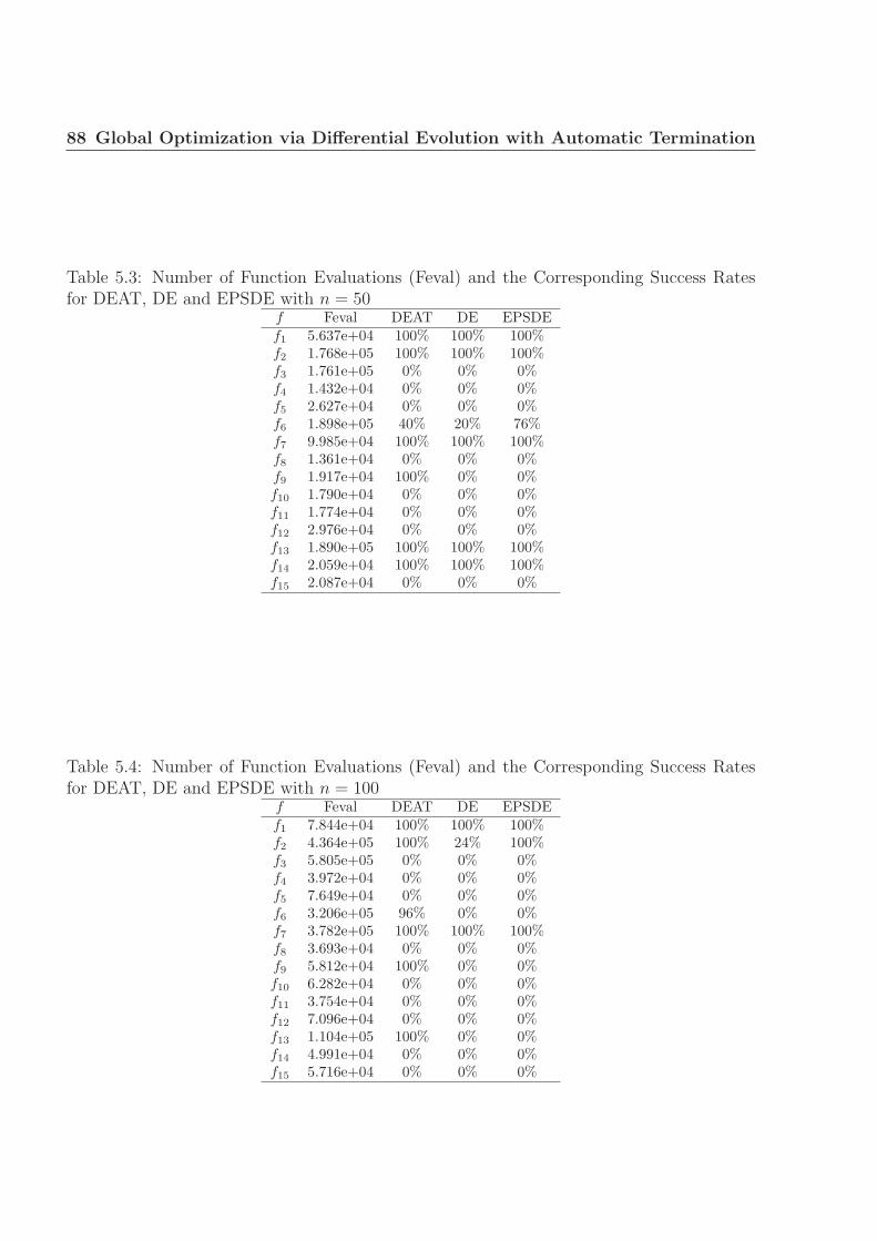
88 Global Optimization via Differential Evolution with Automatic Termination
Table 5.3: Number of Function Evaluations (Feval) and the Corresponding Success Ratesfor DEAT, DE and EPSDE with n = 50
f Feval DEAT DE EPSDEf1 5.637e+04 100% 100% 100%f2 1.768e+05 100% 100% 100%f3 1.761e+05 0% 0% 0%f4 1.432e+04 0% 0% 0%f5 2.627e+04 0% 0% 0%f6 1.898e+05 40% 20% 76%f7 9.985e+04 100% 100% 100%f8 1.361e+04 0% 0% 0%f9 1.917e+04 100% 0% 0%f10 1.790e+04 0% 0% 0%f11 1.774e+04 0% 0% 0%f12 2.976e+04 0% 0% 0%f13 1.890e+05 100% 100% 100%f14 2.059e+04 100% 100% 100%f15 2.087e+04 0% 0% 0%
Table 5.4: Number of Function Evaluations (Feval) and the Corresponding Success Ratesfor DEAT, DE and EPSDE with n = 100
f Feval DEAT DE EPSDEf1 7.844e+04 100% 100% 100%f2 4.364e+05 100% 24% 100%f3 5.805e+05 0% 0% 0%f4 3.972e+04 0% 0% 0%f5 7.649e+04 0% 0% 0%f6 3.206e+05 96% 0% 0%f7 3.782e+05 100% 100% 100%f8 3.693e+04 0% 0% 0%f9 5.812e+04 100% 0% 0%f10 6.282e+04 0% 0% 0%f11 3.754e+04 0% 0% 0%f12 7.096e+04 0% 0% 0%f13 1.104e+05 100% 0% 0%f14 4.991e+04 0% 0% 0%f15 5.716e+04 0% 0% 0%

5.3 Numerical Results 89
5.3.3 Comparison with DE
To evaluate the performance of DEAT against DE, we first let DEAT run until it terminates
automatically and then compute its success rates for each function. Afterward, by using
the same amount of objective function evaluations for each function as the termination
condition, the success rates obtained by the compared method are determined. Results are
reported in Tables 5.2, 5.3 and 5.4, in 10, 50 and 100 dimensions, respectively. For each test
function, the numbers of function evaluations needed by DEAT and DE are shown as well
as the success rate for each function.
In 10 dimensions, we can observe via Table 5.2 that both DEAT and DE could solve
exactly the same functions, 11 out of 15. Only functions f4, f5, f8 and f15 could not be
solved under the specified accuracy level. Success rates are around the same order. In 50
dimensions, DEAT could reach or be close enough to a global optimum on 7 functions, while
DE could find it on 6 functions out of 15, as reported in Table 5.3. In particular, function
f9 could be solved at each attempt by DEAT but never by DE. We note that all the other
functions that DE could handle were also so by DEAT. Moreover, function f6 has a success
rate that is double for DEAT compared to DE. In 100 dimensions, as shown in Table 5.4,
the gap between the two methods gets bigger. DEAT could work out a solution under the
accuracy level on 6 functions, but DE could only do it for 3 functions out of the 15 functions.
Additionally, the success rate for function f2 is 4 times lower for DE, while DEAT could find
the optimal solution at each run.
5.3.4 Comparison with EPSDE
In this section, DEAT is compared against a recent state-of-the-art algorithm called EPSDE
that uses an ensemble of mutation strategies and parameter values with DE (Mallipeddi
et al., 2011). This method makes use of a set of mutation strategies with different parameter
settings and thus avoids unique parameter settings as in the classical DE. Since different
strategies may become more effective during the evolution process than others depending on
the problem, EPSDE keeps a pool of mutation strategies and parameters that have diverse
characteristics in an attempt to adapt to different stage of the evolution process and to the
nature of a particular problem. In (Mallipeddi et al., 2011), EPSDE is favorably compared
to several well-known state-of-the-art DE methods.
Results are stated in Tables 5.2, 5.3 and 5.4, in 10, 50 and 100 dimensions, respectively. In
10 dimensions, we can observe that DEAT could solve more functions (functions f4 anf f12)
and more efficiently (functions f2, f6, f10 and f11) than EPSDE. In 50 dimensions, DEAT
performed slightly better, since it could solve one more function (function f9), although
the success rate for function f6 is higher for EPSDE. Success rates in 100 dimensions show,
however, that DEAT clearly outperformed EPSDE by successfully solving 6 functions against

90 Global Optimization via Differential Evolution with Automatic Termination
3 for EPSDE.
Those findings from the comparison of DEAT against DE and EPSDE indicate that SD
and SR have beneficial effects on the performance of DE for high dimensional problems.
Coupled with the GM, those mechanisms could determine a termination instant without
deteriorating the performance of the algorithm.
5.4 Conclusion
In this chapter, we have proposed to combine DE with the GM, SR and SD mechanisms
in order to equip DE with an automatic termination strategy that does not require any
prescribed criterion such as the maximum number of generations or function evaluations.
The search aims at exploring widely the whole search space, which is sequentially decom-
posed into two-dimensional subspaces that undergo a series of rotations, thereby avoiding
premature convergence and termination of the search.
Numerical experiments conducted on a set of 15 test functions presented at the CEC
2005 in 10, 50 and 100 dimensions reveal that the results obtained by DEAT are equal
or superior to those of the classical DE and the recent EPSDE, without undue objective
function evaluations and without negative impact on the quality of the solution obtained.

Chapter 6
Automatically Terminated ParticleSwarm Optimization with PrincipalComponent Analysis
In this chapter, a hybrid PSO that features an automatic termination and better search
efficiency than classical PSO is presented. The proposed method is combined with the
GM to provide the search with a self-check in order to determine a proper termination
instant. Its convergence speed and reliability are also increased by the implementation
of the Principal Component Analysis technique and the hybridization with a local search
method. The proposed algorithm is denominated as Automatically Terminated Particle
Swarm Optimization with Principal Component Analysis (AT-PSO-PCA). The computa-
tional experiments demonstrate the effectiveness of the automatic termination criteria and
show that AT-PSO-PCA enhances the convergence speed, accuracy and reliability of the
PSO paradigm. Furthermore, comparisons with state-of-the-art evolutionary algorithms
yield competitive results even under the automatically detected termination instant.
6.1 Introduction
Improving the performance of the GM has been performed in Chapter 4 by developing the SD
and SR mechanisms. In this chapter, we show that implementing other techniques and taking
advantage of the inner structure of the host EC method can also yield improved performance.
Here, the PSO paradigm, as an example of SI method in considered. To materialize the
automatic termination, we equip PSO with the GM, described in Section 2.4. The GM is a
matrix that represents subranges of the possible values of each variable. It gives an indication
on the distributions of the variables over the search range. This information is used to provide
the search with new diverse solutions and let the search know how far the exploration process
has been performed. Along with a self-check to determine a proper termination instant, the

92Automatically Terminated Particle Swarm Optimization with Principal
Component Analysis
proposed method also attempts to improve both convergence speed and reliability at the
same time. To do so, we utilize the Principal Component Analysis (PCA) technique. At each
iteration, PCA operates on each particle’s pbest (that comprises a set of possibly correlated
variables) in order to extract the eigenvectors that will be used to transform the original
search space into an alternative space that possesses a new coordinate system wherein the
swarm can navigate through uncorrelated dimensions. Finally, to further accelerate the
search process, a local search method is used to improve the gbest candidate solution obtained
upon GM termination. We call the proposed method Automatically Terminated Particle
Swarm Optimization with Principal Component Analysis, abbreviated as AT-PSO-PCA.
The performance of AT-PSO-PCA is evaluated through numerical experiments on a set of
widely used test problems and compared against the classical PSO as well as a number
of existing methods such as the Fully Informed Particle Swarm optimizer (FIPS) (Mendes
et al., 2004), the state-of-the-art Comprehensive Learning Strategy PSO (CLPSO) (Liang
et al., 2006), and the two state-of-the-art EAs called the Differential Evolution Algorithm
with Ensemble of Parameters and Mutation Strategies (EPSDE) (Mallipeddi et al., 2011)
and the Global and Local Real-Coded Genetic Algorithm based on Parent-Centric Crossover
Operators (GL-25) (Garcıa-Martinez et al., 2008).
AT-PSO-PCA seeks an optimal or near-optimal solution of the nonconvex optimization
problem defined in Section 1.1.
The rest of this chapter is organized as follows. In Section 6.2, the proposed techniques
that compose AT-PSO-PCA are presented. Section 6.3 provides the experiments and com-
parative study conducted and discusses the results. The individual effect of PCA on the
performance of PSO is analyzed in Section 6.4. The concluding remarks are given in Section
6.5.
6.2 AT-PSO-PCA Mechanisms
In AT-PSO-PCA, the GM and mutagenesis operator are implemented as in G3AT. Their
description is provided in Section 2.4. The rest of this section reviews the PCA technique
and describes the AT-PSO-PCA algorithm in detail.
6.2.1 Principal Component Analysis
PCA (Jolliffe, 1986) is a mathematical technique widely used in various fields such as neuro-
science, pattern recognition and image compression. It employs an orthogonal linear trans-
formation to extract a set of values of uncorrelated variables from a set of possibly correlated
variables. The created set of variables is called the “principal components” and their num-
ber is less than or equal to the number of original variables. Applications take advantage of

6.2 AT-PSO-PCA Mechanisms 93
PCA to reduce complex or confusing data sets into lower dimensions without much loss of
information to simplify the identification of patterns in data or reveal their similarities and
differences.
Let X be an n×µ matrix with zero empirical mean that contains a data set of µ objects
with n variables. We assume n < µ. In our proposed PSO, X represents a swarm consisting
of µ particles in Rn. More specifically, each column of X is the position of a particle. The
singular value decomposition of X is expressed as
X = WΣV T , (6.2.1)
where T denotes transpose, W is the n× n matrix of eigenvectors of XXT , V is the µ× µ
matrix of eigenvectors of XT X,
Σ =
σ1
. . . 0σn
is an n× µ rectangular diagonal matrix with nonnegative diagonal entries σ1 ≥ σ2 ≥ . . . ≥σn ≥ 0. By defining the n × L matrix WL as the matrix that consists of the first L (≤ n)
columns of W , the operation
Y = W TL X (6.2.2)
will project X onto the reduced subspace defined by WL to form the L× µ matrix Y . The
reverse operation is performed with
X = WLY. (6.2.3)
In the Euclidean space, PCA can be seen as an operator that rotates the original axes to
new positions (called the principal axes) such that, among other properties, the covariance
among each pair of the principal axes is zero.
6.2.2 AT-PSO-PCA Formal Algorithm
Our proposed method combines PSO with three distinct components (GM, PCA and a
local search) to pursue the following three objectives. The first objective is to equip PSO
with an intelligent automatic termination criterion. The second objective is to enhance the
convergence speed of the search. At the same time, the last and third objective is to improve
the reliability of the algorithm. To fulfill them, the proposed method is equipped with the
Simple GM described in Section 2.4. When the GM indicates that a sufficient exploration
has been performed (i.e., when all the entries of GM are non-null), the search is terminated.
The GM also participates in fulfilling the second objective by providing some individuals
with the ability to “jump” towards apparently unexplored area of the search space by using

94Automatically Terminated Particle Swarm Optimization with Principal
Component Analysis
mutagenesis. This mechanism is also a guarantee that the search will eventually stop. To
further enhance the convergence speed, the final intensification process calls a local search
method based on the Kelley’s modification (Kelley, 1999) of the Nelder-Mead (NM) method
(Nelder and Mead, 1965). The local search is initiated from the gbest obtained at the end
of the search. AT-PSO-PCA thus behaves like a “Memetic Algorithm” (Moscato, 1999; Le
et al., 2009) in order to achieve faster convergence (Ong et al., 2006; Kramer, 2010). For the
third objective, the reliability of the algorithm is improved by creating a gbest of high quality
after the automatic termination for undertaking the final intensification process. This role
is carried out by the PCA operation described in Subsection 6.2.1 which operates during
the search by transforming the coordinates of the search space into a different coordinate
system of dimension L at every iteration. In AT-PSO-PCA, this is achieved by extracting the
principal components of the set composed by all the pbests. Then, the new set of coordinates
is created from an orthogonal transformation that uses the obtained principal components.
Afterwards, the swarm navigates through the “distorted dimensions” and new positions are
computed. Finally, the obtained positions are transformed back into the original space and
form a candidate swarm S. Each particle of the swarm S is given a chance to undertake
a random p-point (p < n) crossover operation of probability πc with gbest. If the function
value of the resulting particle is better than or equal to the function value of the pbest of
the corresponding particle in the original space, then the obtained particle becomes the new
pbest. The AT-PSO-PCA pseudocode is described in Algorithm 6.2.1.
Algorithm 6.2.1. AT-PSO-PCA Pseudocode
1. Initialization. For each particle pi in the swarm, i = 1, . . . , µ, do thefollowing:1.1. Initialize xi and vi randomly.1.2. Evaluate f(xi).1.3. Initialize pbesti associated to pi.1.4. Initialize GM as the n×m zero matrix.
2. Main loop. Repeat Steps 2.1 to 2.7 until GM reaches the completion ratioCP .2.1. Locate gbest.2.2. For each particle pi, set pbesti := xi if f(xi) ≤ f(pbesti).2.3. For each particle pi, update xi and vi by applying Equations (1.5.1) and(1.5.2).2.4. GM. Update GM and perform mutagenesis by applying Procedure 2.4.1to alter the µw (≤ µ) worst particles.2.5. PCA. Apply Equation (6.2.1) with the set of pbests with zero empiricalmean and extract the matrix WL. Apply Equation (6.2.2) with the swarm Xto form the matrix of particles Y . Update the position of each particle in Ywith Equation (1.5.1). Apply Equation (6.2.3) to transform Y back into theoriginal space and form the candidate swarm S.

6.3 Numerical Experiments 95
2.6. Associate a random number from (0, 1) with each particle si of S. If theassociated number is less than πc, perform a p-point crossover operation withsi and gbest to alter si.2.7. Evaluate f(xi) and f(si). For each particle si in S, set pbesti := si iff(si) ≤ f(pbesti).
3. Intensification. Apply a local search method starting from gbest.
6.3 Numerical Experiments
To validate the performance of AT-PSO-PCA, we have selected a benchmark composed of
11 test functions that are taken from (Yao et al., 1999) and listed in Table 6.1. They provide
a good balance of complexity and modality, and have been widely used by many researchers
(Angeline, 1998a; Shi and Eberhart, 1998; Lovbjerg and Krink, 2002; Esquivel and Coello,
2003; Higashi and Iba, 2003; Richards and Ventura, 2003). Functions f1–f6 are unimodal
functions and functions f7–f11 are multimodal. Furthermore, existing state-of-the-art PSO
and EAs, listed below, were selected to provide a comparison analysis with AT-PSO-PCA:
• SPSO (Kennedy and Eberhart, 1995) (PSO),
• FIPS (Mendes et al., 2004) (PSO),
• CLPSO (Liang et al., 2006) (PSO),
• EPSDE (Mallipeddi et al., 2011) (DE),
• GL-25 (Garcıa-Martinez et al., 2008) (GA).
The first PSO is the standard PSO (Kennedy and Eberhart, 1995) and is here abbreviated
as SPSO. FIPS (Mendes et al., 2004) is a PSO that uses all the particles in the swarm to
update the velocity vector. It is a so-called “fully informed” PSO. To improve its success
rate, Mendes et al. recommend the use of a URing topology structure with weighted FIPS
based on the goodness algorithm (Mendes et al., 2004). CLPSO (Liang et al., 2006) uses
a “comprehensive learning strategy” that was developed to improve the performance of
PSO on multimodal functions. EPSDE is a recent DE that uses an ensemble of mutation
strategies and parameter values (Mallipeddi et al., 2011). This method makes use of a set
of mutation strategies with different parameter settings and thus avoids unique parameter
settings as in the classical DE. Since different strategies may become more effective during the
evolution process than others depending on the problem, EPSDE keeps a pool of mutation
strategies and parameters that have diverse characteristics in an attempt to adapt to different
stages of the evolution process and to the nature of a particular problem. GL-25 (Garcıa-
Martinez et al., 2008) is a GA with improved crossover operators with a male and female

96Automatically Terminated Particle Swarm Optimization with Principal
Component Analysis
Table 6.1: Test Functionsf
Func
tion
Nam
en
Bou
nds
Glo
balM
inE
rror
Tol
f 1(x
)=
∑n i=
1x
2 iSp
here
Mod
el30
[-10
0,10
0]n
00.
01f 2
(x)=
∑n i=
1|x i|+
Πn i=
1|x i|
Schw
efel
’sP
2.22
30[-10
,10]
n0
0.01
f 3(x
)=
∑n i=
1(∑
i j=1x
j)2
Schw
efel
’sP
1.2
30[-10
0,10
0]n
010
0
f 4(x
)=
∑n−1
i=1
[ 100
( x2 i−
xi+
1
) 2+
(xi−
1)2]
Gen
eral
ized
Ros
enbr
ock
30[-10
,10]
n0
100
f 5(x
)=
∑n i=
1(bx
i+
0.5c
)2St
ep30
[-10
0,10
0]n
00
f 6(x
)=
∑n i=
1ix
4 i+
random
[0,1
)Q
uart
icw
ith
Noi
se30
[-1.
28,1
.28]
n0
0.01
f 7(x
)=−
∑n i=
1
( xisi
n√|x i|)
Gen
eral
ized
Schw
efel
’sP
2.26
30[-50
0,50
0]n
-125
69-1
0000
f 8(x
)=
10n
+∑
n i=1
( x2 i−
10co
s(2π
xi)
)G
ener
aliz
edR
astr
igin
30[-5.
12,5
.12]
n0
50f 9
(x)=
14000
∑n i=
1x
2 i−
∏n i=
1co
s( xi √i
) +1
Gen
eral
ized
Gri
ewan
k30
[-60
0,60
0]n
00.
01
f 10(x
)=
20+
e−
20e−
1 5
q1 n
Pn i=
1x2 i
Ack
ley
30[-32
,32]
n0
0.01
−e1 n
Pn i=
1co
s(2πx
i)
f 11(x
)=
∑n−1
i=1(z
1−
1)2(1
+10
sin
2(π
z i+
1))
Gen
eral
ized
Pen
aliz
ed30
[-50
,50]
n0
0.01
+π/3
0(10
sin
2(π
z 1)+
(zn−
1)2)
+∑
n i=1u(x
i,10
,100
,4)
whe
rez
=1
+0.
25(x
i+
1),
u(x
i,a,k
,m)=
k(x
i−
a)m
,x
i>
a;
0,−a
≤x
i≤
a;
k(−
xi−
a)m
,x
i<
a.

6.3 Numerical Experiments 97
Table 6.2: AT-PSO-PCA Parameter SettingParameter Definition Valueµ Size of the swarm 40w Inertia weight 0.72c1 Cognition weight 1.2c2 Social weight 1.2m No. of GM subranges 500µw No. of individuals used by mutagenesis 2CP Completion ratio of GM 90%L Dimension of the reduced subspace 1πc Crossover probability 0.6
differentiation process for each of the parents as well as some new male and female selection
mechanisms. The crossover operators create the offspring in the neighborhood of one of the
parents (the female parent) while the second parent (the male parent) defines the range of
the neighborhood. By adjusting the number of female and male parents that participate in
the differentiation process, GL-25 can act as a global search algorithm or as a local search
algorithm with more or less reliability and accuracy. Throughout our numerical experiments,
the population size is set at 40 for all methods and the adopted parameter settings are those
recommended by their respective authors. The AT-PSO-PCA parameters with their assigned
values are summarized in Table 6.2.
It should be noted that to conduct a fair comparison and due to the main goal of AT-
PSO-PCA, which is to let the search stop automatically, we have adopted in this chapter a
particular comparison framework. Indeed, the comparisons with the existing methods are
conducted in two stages. In the first stage, of which results are reported in Table 6.3, we
compare the best function value, abbreviated as Fmin, obtained by each algorithm for each
function upon termination. In this stage, termination for each method took place with the
number of function evaluations, referred to as Feval, that was required by AT-PSO-PCA
to terminate automatically. It gives an indication on the accuracy and reliability of the
solutions obtained by AT-PSO-PCA upon termination and thus, on the effectiveness of the
proposed termination mechanism. The second stage allows the compared methods to run
longer and show their performance with a predetermined Feval that is considerably bigger
than that in the first stage. Namely, in the second stage, Feval is set equal to 2 × 10⁵ for
all functions and all methods but AT-PSO-PCA that preserves its automatic termination.
Results are reported in Table 6.4. The objective is to detect whether AT-PSO-PCA suffered
or not from premature termination when compared to existing algorithms. In both stages,
the error tolerance levels specified in Table 6.1 (Error Tol) are used to judge if a run is
successful or not. Specifically, a run is considered successful when the fixed error tolerance
level is achieved at the end of the search. The success rate, abbreviated as SRate, is defined

98Automatically Terminated Particle Swarm Optimization with Principal
Component Analysis
as the number of successful runs divided by the total number of independent runs, here equal
to 25 for all methods. Tables 6.3 and 6.4 report the mean Fmin and standard deviation (SD),
as well as the SRate obtained for each test function by each algorithm.
6.3.1 First Stage - Accuracy and Reliability
Table 6.3 lists the performance on the solution accuracy in terms of the mean Fmin, SD
and SRate of each compared method. It can be observed that AT-PSO-PCA generally
obtains quite accurate results upon (automatic) termination. Also, it could achieve the
global optimum with 100% SRate on 10 out of 11 functions and with a non-null SRate for
the remaining function f7. By computing the mean SRate obtained over all test functions, it
appears that AT-PSO-PCA has the highest overall SRate (94%), followed by EPSDE (89%)
and CLPSO (82%). We note that AT-PSO-PCA performs relatively well on both unimodal
functions f1–f6 and multimodal functions f7–f11. Actually, AT-PSO-PCA offers the best
overall performance among all algorithms and only EPSDE, CLPSO and FIPS are superior
when applied to the multimodal function f7. It should also be noted that there is no problem
that could not be solved at all by AT-PSO-PCA.
Those results show that the quality of the solutions obtained by AT-PSO-PCA after its
automatic termination is very competitive. Actually, it achieves some of the best results in
terms of accuracy and reliability on most test functions.
6.3.2 Second Stage - Premature Termination
The results in this stage, as displayed in Table 6.4, show that in terms of accuracy, some
methods get more accurate solutions for some problems than AT-PSO-PCA (especially for
unimodal functions). However, we may claim that, in spite of the fact that AT-PSO-PCA
uses on average 60% less Feval than the other methods, it is still generally competitive.
Furthermore, even though a considerably higher Feval is allowed to the other algorithms,
AT-PSO-PCA with its relatively small Feval still has the best overall SRate (94%). Indeed,
although the overall SRate of some of the rival methods (FIPS and GL-25) increased signif-
icantly, the second highest overall SRate is once again obtained by EPSDE with an overall
SRate that is now of 91%. This demonstrates that the use of the automatic termination did
not have negative effect on the quality of the solutions achieved by AT-PSO-PCA.
6.4 Impact of PCA
The impact of the GM and the intensification phase (local search) has been discussed in
Section 4.3.5. It is shown that the use of GM effectively assists an algorithm to achieve wide
exploration and deep exploitation before stopping the search. Moreover, the intensification

6.4 Impact of PCA 99
Table 6.3: Fmin Obtained by Each Method after the Same Feval as AT-PSO-PCA
Fm
inm
ean
(SR
ate)
fFe
valm
ean
AT
-PSO
-PC
ASP
SOFIP
SC
LP
SOE
PSD
EG
L-2
5f 1
8.58
e+04
1.95
e-82
(100
%)
4.78
e-54
(100
%)
2.39
e-03
(100
%)
1.17
e-05
(100
%)
9.06
e-55
(100
%)
7.00
e-19
(100
%)
f 28.
60e+
046.
15e-
43(1
00%
)1.
89e+
00(0
%)
7.72
e-03
(96%
)1.
66e-
04(1
00%
)7.
75e-
27(1
00%
)1.
45e-
10(1
00%
)f 3
8.59
e+04
2.67
e-80
(100
%)
1.14
e-04
(100
%)
2.43
e+03
(0%
)2.
83e+
03(0
%)
6.02
e+01
(96%
)1.
56e+
03(0
%)
f 48.
73e+
042.
68e+
01(1
00%
)2.
50e+
01(1
00%
)2.
71e+
01(1
00%
)6.
19e+
01(1
00%
)2.
02e+
00(1
00%
)2.
33e+
01(1
00%
)f 5
9.02
e+04
0.00
e+00
(100
%)
1.08
e+00
(40%
)0.
00e+
00(1
00%
)0.
00e+
00(1
00%
)1.
60e-
01(8
4%)
8.40
e-01
(36%
)f 6
8.62
e+04
3.98
e-02
(100
%)
5.09
e-01
(100
%)
1.42
e-02
(0%
)1.
20e-
02(0
%)
3.48
e-03
(0%
)1.
92e-
02(0
%)
f 74.
11e+
04-9
.07e
+03
(36%
)-7
.03e
+03
(0%
)-1
.25e
+04
(100
%)
-1.2
6e+
04(1
00%
)-1
.26e
+04
(100
%)
-4.0
8e+
03(0
%)
f 88.
63e+
040.
00e+
00(1
00%
)2.
94e+
01(8
4%)
1.02
e+02
(0%
)5.
79e+
00(1
00%
)1.
42e-
16(1
00%
)1.
43e+
02(1
2%)
f 98.
51e+
040.
00e+
00(1
00%
)6.
99e-
03(7
6%)
2.83
e-02
(12%
)4.
55e-
04(1
00%
)0.
00e+
00(1
00%
)2.
96e-
04(1
00%
)f 1
08.
49e+
048.
88e-
16(1
00%
)9.
75e-
01(2
8%)
1.29
e-02
(8%
)1.
36e-
03(1
00%
)7.
28e-
15(1
00%
)5.
28e-
10(1
00%
)f 1
18.
60e+
042.
39e-
18(1
00%
)4.
15e-
02(7
2%)
1.15
e-04
(100
%)
4.99
e-07
(100
%)
4.15
e-03
(96%
)8.
23e-
22(1
00%
)
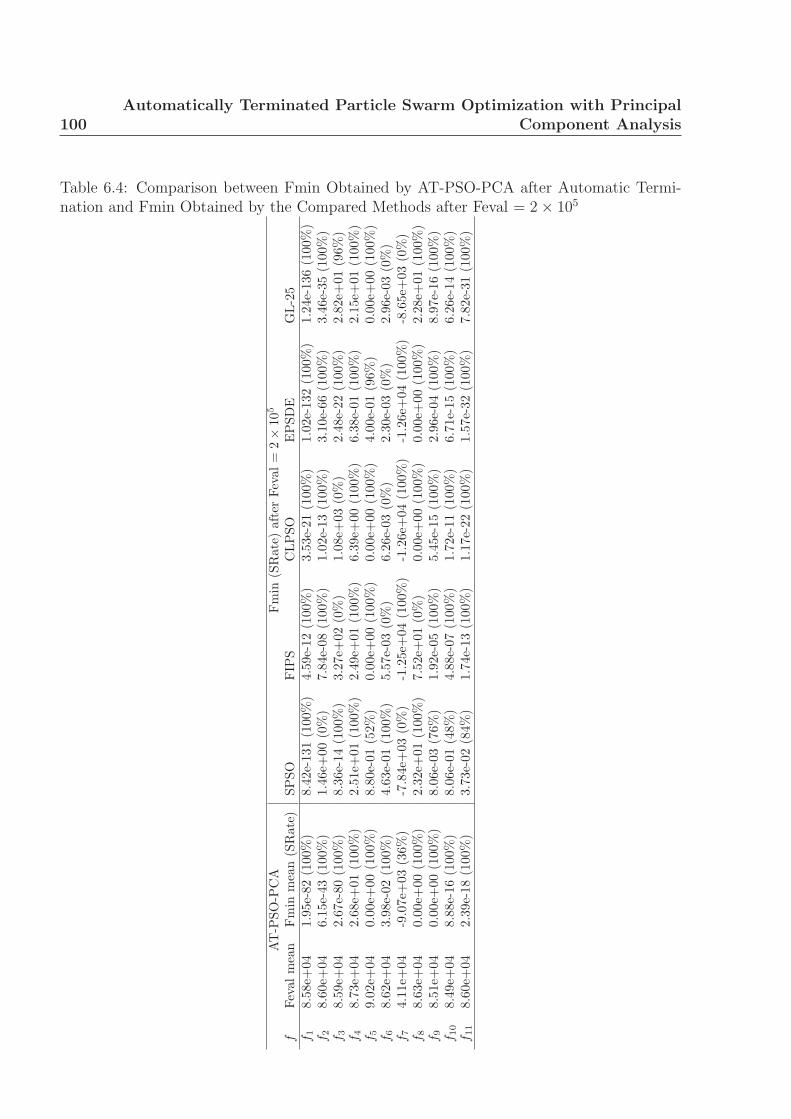
100Automatically Terminated Particle Swarm Optimization with Principal
Component Analysis
Table 6.4: Comparison between Fmin Obtained by AT-PSO-PCA after Automatic Termi-nation and Fmin Obtained by the Compared Methods after Feval = 2× 10⁵
AT
-PSO
-PC
AFm
in(S
Rat
e)af
ter
Feva
l=
2×
105
fFe
valm
ean
Fm
inm
ean
(SR
ate)
SPSO
FIP
SC
LP
SOE
PSD
EG
L-2
5f 1
8.58
e+04
1.95
e-82
(100
%)
8.42
e-13
1(1
00%
)4.
59e-
12(1
00%
)3.
53e-
21(1
00%
)1.
02e-
132
(100
%)
1.24
e-13
6(1
00%
)f 2
8.60
e+04
6.15
e-43
(100
%)
1.46
e+00
(0%
)7.
84e-
08(1
00%
)1.
02e-
13(1
00%
)3.
10e-
66(1
00%
)3.
46e-
35(1
00%
)f 3
8.59
e+04
2.67
e-80
(100
%)
8.36
e-14
(100
%)
3.27
e+02
(0%
)1.
08e+
03(0
%)
2.48
e-22
(100
%)
2.82
e+01
(96%
)f 4
8.73
e+04
2.68
e+01
(100
%)
2.51
e+01
(100
%)
2.49
e+01
(100
%)
6.39
e+00
(100
%)
6.38
e-01
(100
%)
2.15
e+01
(100
%)
f 59.
02e+
040.
00e+
00(1
00%
)8.
80e-
01(5
2%)
0.00
e+00
(100
%)
0.00
e+00
(100
%)
4.00
e-01
(96%
)0.
00e+
00(1
00%
)f 6
8.62
e+04
3.98
e-02
(100
%)
4.63
e-01
(100
%)
5.57
e-03
(0%
)6.
26e-
03(0
%)
2.30
e-03
(0%
)2.
96e-
03(0
%)
f 74.
11e+
04-9
.07e
+03
(36%
)-7
.84e
+03
(0%
)-1
.25e
+04
(100
%)
-1.2
6e+
04(1
00%
)-1
.26e
+04
(100
%)
-8.6
5e+
03(0
%)
f 88.
63e+
040.
00e+
00(1
00%
)2.
32e+
01(1
00%
)7.
52e+
01(0
%)
0.00
e+00
(100
%)
0.00
e+00
(100
%)
2.28
e+01
(100
%)
f 98.
51e+
040.
00e+
00(1
00%
)8.
06e-
03(7
6%)
1.92
e-05
(100
%)
5.45
e-15
(100
%)
2.96
e-04
(100
%)
8.97
e-16
(100
%)
f 10
8.49
e+04
8.88
e-16
(100
%)
8.06
e-01
(48%
)4.
88e-
07(1
00%
)1.
72e-
11(1
00%
)6.
71e-
15(1
00%
)6.
26e-
14(1
00%
)f 1
18.
60e+
042.
39e-
18(1
00%
)3.
73e-
02(8
4%)
1.74
e-13
(100
%)
1.17
e-22
(100
%)
1.57
e-32
(100
%)
7.82
e-31
(100
%)

6.4 Impact of PCA 101
Table 6.5: Fmin Obtained by SPSO and PSO-PCA after Feval = 105
Fmin mean (SRate)f Feval mean SPSO PSO-PCAf1 1.00e+05 2.02e-63 (100%) 1.05e-99 (100%)f2 1.00e+05 1.25e+00 (0%) 5.69e-51 (100%)f3 1.00e+05 1.26e-05 (100%) 1.11e-99 (100%)f4 1.00e+05 3.18e+01 (100%) 2.65e+01 (100%)f5 1.00e+05 5.20e-01 (48%) 0.00e+00 (100%)f6 1.00e+05 4.85e-01 (100%) 5.32e-01 (100%)f7 1.00e+05 -7.55e+03 (0%) -9.01e+03 (40%)f8 1.00e+05 3.28e+01 (84%) 0.00e+00 (100%)f9 1.00e+05 4.83e-03 (68%) 0.00e+00 (100%)f10 1.00e+05 8.79e-01 (32%) 8.88e-16 (100%)f11 1.00e+05 2.49e-02 (76%) 6.98e-22 (100%)
(a) Function f1 (b) Function f11
Figure 6.1: Convergence performance of SPSO and PSO-PCA on (a) function f1 and (b)function f11.
serves as a mechanism that increases the exploitation power of an algorithm, but when used
alone, it cannot achieve the results obtained by its combination with its host algorithm.
Here, we investigate how the implementation of the PCA technique within the canonical
PSO (SPSO) affects the performance of the method. We also analyze the influence of
the parameter L that determines the number of dimensions in the new coordinate system
generated by PCA.
6.4.1 PCA within SPSO
We carried out comparative experiments that consisted in confronting SPSO against the
classical PSO with PCA, referred to as PSO-PCA. Compared to AT-PSO-PCA, PSO-PCA

102Automatically Terminated Particle Swarm Optimization with Principal
Component Analysis
(a) Accuracy (b) Computational cost
Figure 6.2: Effect of the parameter L ranging between 1 and n (= 30) on function f1 interms of (a) Accuracy log(Fmin) and (b) Computational cost Feval.
does not contain the GM, mutagenesis and the final intensification phase. Consequently,
PSO-PCA is not equipped with an automatic termination.
Comparisons are made using the same benchmark functions listed in Table 6.1, as in
Section 6.3. Both SPSO and PSO-PCA are terminated after 100,000 objective function
evaluations. The average Fmin and SRate over 25 independent runs are reported in Table
6.5. Figure 6.1 graphically presents the comparisons in terms of log(Fmin) over Feval for
functions f1 and f11, as examples of an unimodal function and a multimodal function,
respectively. Figure 6.1(a) depicts the convergence speed of SPSO and PSO-PCA when
minimizing f1, a relatively easy unimodal function. The figure shows that PSO-PCA has a
higher convergence speed than SPSO. Furthermore, in some cases such as the one depicted
in Figure 6.1(b), where both methods are minimizing f11, a complex multimodal function,
it can be observed that SPSO got stuck at local minima after around 2× 10⁴ Fevals. On the
other hand, PSO-PCA could easily escape from local optima and attain a global optimum.
In terms of SRate, PSO-PCA evidently outperforms SPSO on the unimodal functions and
also on the complex multimodal functions. In particular, a global optimum for function f2
could not be found at all by SPSO, while the same problem was solved with a 100% success
rate by PSO-PCA.
Those observations suggest that SPSO benefits from the use of PCA by attaining global
minima for both unimodal and multimodal functions, with increased reliability. The use of
PCA can increase the ability of SPSO to jump out of local optima and detect global optima.
6.4.2 Effect of Parameter L
In AT-PSO-PCA, the role of the parameter L is to control the number of dimensions of
the space on which the swarm is projected. To assess the influence of L, we have tested

6.5 Conclusion 103
(a) Accuracy (b) Computational cost
Figure 6.3: Effect of the parameter L ranging between 1 and n (= 30) on function f10 interms of (a) Accuracy log(Fmin) and (b) Computational cost Feval.
AT-PSO-PCA with different numbers of L ranging between 1 and n. Figures 6.2 and 6.3
depict the results obtained for functions f1 and f10, respectively, as examples of an unimodal
function and a multimodal function, with n = 30.
We can observe that both f1 and f10 behave in a similar way in terms of Fmin and Feval.
Indeed, in Figures 6.2(a) and 6.3(a), we see that log(Fmin) decreases as L decreases. For
functions f1 and f10, log(Fmin) is equivalent to log(Error) and is thus an indicator of the
accuracy of the search, i.e., the smaller log(Fmin), the higher the accuracy. The improvement
in terms of accuracy is particularly high for the unimodal function f1. However, Figures
6.2(b) and 6.3(b) reveal that Feval increases as L decreases. Nevertheless, the authors believe
that the growth in Feval is relatively low when compared to the improvement achieved in
terms of accuracy. In our experiments, there were no problems for which reducing L led to
less accurate results. In the worst case, only Feval increased for the same accuracy. Those
findings show that AT-PSO-PCA is able to take advantage of the principal components that
have the highest variance to increase effectively the accuracy of the search under acceptable
augmentation of the cost in terms of Feval.
6.5 Conclusion
In this chapter, we have introduced a new PSO, called AT-PSO-PCA, that is equipped with
an automatic termination criterion based on the GM in order to terminate the search without
conventional predefined criteria while avoiding premature termination. It also uses the PCA
technique and a local search process to enhance the quality of the obtained solutions in terms
of accuracy and reliability. PCA creates a search space based on the principal components
of the set of all pbests. In that search space of possibly reduced dimension navigates the
swarm to locate new promising areas. In the original set of coordinates, it forms a candidate

104Automatically Terminated Particle Swarm Optimization with Principal
Component Analysis
swarm that is given a chance to replace some of the pbests of the original swarm at each
iteration.
Numerical experiments carried out on a set of widely used test functions and comparisons
with state-of-the-art methods have shown that AT-PSO-PCA is competitive and that the
main objectives have been fulfilled. Indeed, for all test functions, our proposed method could
achieve very competitive results under a limited amount of function evaluations, without
falling into premature termination or requiring undue objective function evaluations. In
terms of accuracy and reliability, AT-PSO-PCA also clearly outperforms the canonical PSO
and is comparable or superior to many of the well-known PSO and EAs. These results
suggest that AT-PSO-PCA can contribute to real-world applications of PSO.

Chapter 7
Summary and Conclusions
In this dissertation, two subsets of EC have been considered to develop novel methods that
answer the question of the termination criteria for EC. Namely, the proposed methods in
this study are the G3AT, GATR, DEAT and AT-PSO-PCA methods, detailed in Chapters
3–6, respectively. They deal with the nonconvex global optimization problem defined in
Section 1.1. The common elements in our proposed algorithms are the GM, the mutagenesis
operator and the final intensification process. In addition, we have also developed the SD and
SR mechanisms in GATR and implemented the PCA technique in AT-PSO-PCA. We have
shown that our proposed methods can effectively terminate the search without conventional
predefined criteria, without negative impact on the quality of the solution obtained and that
they are comparable or superior to many well-known EC methods.
Specifically, in Chapter 3, we have shown that G3AT is robust and able to reach global
minima or at least be very close to them in many of the selected test problems. The use of
the GM effectively assists the algorithm to achieve wide exploration and deep exploitation
before stopping the search. This indicates that our main objective to equip a GA with an
automatic termination criterion has largely been fulfilled.
In Chapter 4, we have pointed out that as a two-dimensional structure, there is no evi-
dence that the GM is able to represent the distribution of individuals in a multi-dimensional
search space accurately. It has prompted us to develop the SR and SD mechanisms to alle-
viate this drawback and to implement them in GATR. We have shown that GATR can also
terminate the search without conventional predefined criteria and that GATR is significantly
superior to G3AT as well as to many other advanced EAs.
In Chapter 5, we have shown that the GM, SD and SR mechanisms can be success-
fully applied to DE, as an example of another EA. Numerical results have indicated that
DE largely benefits from our developed mechanisms by stopping the search without undue
objective function evaluations and without negative impact on the quality of the solution
obtained.
In Chapter 6, we have shown that the GM can be combined with more traditional

106 Summary and Conclusions
mathematical tools to improve the performance of an EC method. The PSO paradigm was
chosen and the GM was combined with the PCA mathematical technique. Our tests have
shown that the resulting method was successfully equipped with an automatic termination
criterion and could outperform the canonical PSO. Also, we have shown that AT-PSO-PCA
is comparable or superior to many well-known PSO and EAs.
Although our main goal to develop automatic termination criteria for EC has been ful-
filled, there remain topics that deserve further investigations. One of the main questions
that remain unresolved is the number of subranges of the GM. The number of subranges is
seen as a parameter, such as the crossover rate or the size of the initial population. However,
we believe that its value can be determined during the search, for example, by letting the
algorithm estimate the landscape of the function being optimized and by setting the number
of subranges according to the estimated complexity of the function. Another question is
the importance of the final intensification process. Finding a mechanism that would fully
combine the local search with the GM is another interesting topic to explore in the future.

Appendix A
Standard Test Functions
Sphere Function (f1)
Definition: f1(x) =∑n
i=1 x2i .
Search space: −100 ≤ xi ≤ 100, i = 1, . . . , n
Global minimum: x∗ = (0, . . . , 0), f1(x∗) = 0.
Schwefel Function (f2)
Definition: f2(x) =∑n
i=1 |xi|+ Πni=1|xi|.
Search space: −10 ≤ xi ≤ 10, i = 1, . . . , n
Global minimum: x∗ = (0, . . . , 0), f2(x∗) = 0.
Schwefel Function (f3)
Definition: f3(x) =∑n
i=1(∑i
j=1 xj)2.
Search space: −100 ≤ xi ≤ 100, i = 1, . . . , n
Global minimum: x∗ = (0, . . . , 0), f3(x∗) = 0.
Schwefel Function (f4)
Definition: f4(x) = maxi=1,...n{|xi|}.Search space: −100 ≤ xi ≤ 100, i = 1, . . . , n
Global minimum: x∗ = (0, . . . , 0), f4(x∗) = 0.
Rosenbrock Function (f5)
Definition: f5(x) =∑n−1
i=1
[100 (x2
i − xi+1)2+ (xi − 1)2
].
Search space: −30 ≤ xi ≤ 30, i = 1, 2, . . . , n.
Global minimum: x∗ = (1, . . . , 1), f5(x∗) = 0.
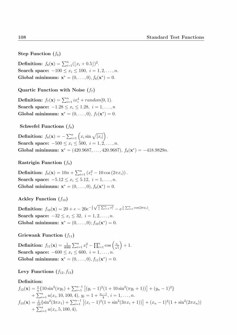
108 Standard Test Functions
Step Function (f6)
Definition: f6(x) =∑n
i=1(bxi + 0.5c)2.
Search space: −100 ≤ xi ≤ 100, i = 1, 2, . . . , n.
Global minimum: x∗ = (0, . . . , 0), f6(x∗) = 0.
Quartic Function with Noise (f7)
Definition: f7(x) =∑n
i=1 ix4i + random[0, 1).
Search space: −1.28 ≤ xi ≤ 1.28, i = 1, . . . , n
Global minimum: x∗ = (0, . . . , 0), f7(x∗) = 0.
Schwefel Functions (f8)
Definition: f8(x) = −∑ni=1
(xi sin
√|xi|
).
Search space: −500 ≤ xi ≤ 500, i = 1, 2, . . . , n.
Global minimum: x∗ = (420.9687, . . . , 420.9687), f8(x∗) = −418.9829n.
Rastrigin Function (f9)
Definition: f9(x) = 10n +∑n
i=1 (x2i − 10 cos (2πxi)) .
Search space: −5.12 ≤ xi ≤ 5.12, i = 1, . . . , n.
Global minimum: x∗ = (0, . . . , 0), f9(x∗) = 0.
Ackley Function (f10)
Definition: f10(x) = 20 + e− 20e−15
√1n
Pni=1 x2
i − e1n
Pni=1 cos(2πxi).
Search space: −32 ≤ xi ≤ 32, i = 1, 2, . . . , n.
Global minimum: x∗ = (0, . . . , 0); f10(x∗) = 0.
Griewank Function (f11)
Definition: f11(x) = 14000
∑ni=1 x2
i −∏n
i=1 cos(
xi√i
)+ 1.
Search space: −600 ≤ xi ≤ 600, i = 1, . . . , n.
Global minimum: x∗ = (0, . . . , 0), f11(x∗) = 0.
Levy Functions (f12, f13)
Definition:
f12(x) = πn{10 sin2(πy1) +
∑n−1i=1
[(yi − 1)2(1 + 10 sin2(πyi + 1))
]+ (yn − 1)2}
+∑n
i=1 u(xi, 10, 100, 4), yi = 1 + xi−14
, i = 1, . . . , n.
f13(x) = 110{sin2(3πx1) +
∑n−1i=1
[(xi − 1)2(1 + sin2(3πxi + 1))
]+ (xn − 1)2(1 + sin2(2πxn))
+∑n
i=1 u(xi, 5, 100, 4),

109
u(xi, a, k,m) =
k(xi − a)m, xi > a;0, −a ≤ xi ≤ a;k(−xi − a)m, xi < a.
Search space: −50 ≤ xi ≤ 50, i = 1, . . . , n.
Global minimum: x∗ = (1, . . . , 1), f12(x∗) = f13(x
∗) = 0.
Shekel Foxholes Function (f14)
Definition: f14(x) =[
1500
+∑25
j=11
j+P2
i=1(xi−Aij)6
]−1
,
A =[ −32 −16 0 16 33 −32 . . . 0 16 32−32 −32 −32 −32 −32 −16 . . . 32 32 32
].
Search space: −65.536 ≤ xi ≤ 65.536, i = 1, 2.
Global minimum: x∗ = (−32,−32); f14(x∗) = 0.998.
Kowalik Function (f15)
Definition: f15(x) =∑11
i=1
[ai − x1(b2i +bix2)
b2i +bix3+x4
]2
,
a = (0.1957, 0.1947, 0.1735, 0.16, 0.0844, 0.0627, 0.0456, 0.0342, 0.0323, 0.0235, 0.0246),
b = (4, 2, 1, 12, 1
4, 1
6, 1
8, 1
10, 1
12, 1
14, 1
16) .
Search space: −5 ≤ xi ≤ 5, i = 1, . . . , 4.
Global minimum: x∗ ≈ (0.1928, 0.1908, 0.1231, 0.1358), f15(x∗) ≈ 0.000375.
Hump Function (f16)
Definition: f16(x) = 4x21 − 2.1x4
1 + 13x6
1 + x1x2 − 4x22 + 4x4
2.
Search space: −5 ≤ xi ≤ 5, i = 1, 2.
Global minima: x∗ = (0.0898,−0.7126), (−0.0898, 0.7126); f16(x∗) = 0.
Branin RCOS Function (f17)
Definition: f17(x) = (x2 − 54π2 x
21 + 5
πx1 − 6)2 + 10(1− 1
8π) cos(x1) + 10.
Search space: −5 ≤ x1 ≤ 10, 0 ≤ x2 ≤ 15.
Global minima: x∗ = (−π, 12.275), (π, 2.275), (9.42478, 2.475); f17(x∗) = 0.397887.
Goldstein & Price Function (f18)
Definition: f18(x) = (1 + (x1 + x2 + 1)2(19− 14x1 + 13x21 − 14x2 + 6x1x2 + 3x2
2))
∗ (30 + (2x1 − 3x2)2(18− 32x1 + 12x2
1 − 48x2 − 36x1x2 + 27x22)).
Search space: −2 ≤ xi ≤ 2, i = 1, 2.
Global minimum: x∗ = (0,−1); f18(x∗) = 3.

110 Standard Test Functions
Hartmann Function (f19)
Definition: f19(x) = −∑4i=1 αi exp
[−∑3
j=1 Aij (xj − Pij)2],
α = [1, 1.2, 3, 3.2]T , A =
3.0 10 300.1 10 353.0 10 300.1 10 35
, P = 10−4
6890 1170 26734699 4387 74701091 8732 5547381 5743 8828
.
Search space: 0 ≤ xi ≤ 1, i = 1, 2, 3.
Global minimum: x∗ = (0.114614, 0.555649, 0.852547); f19(x∗) = −3.86278.
Hartmann Function (f20)
Definition: f20(x) = −∑4i=1 αi exp
[−∑6
j=1 Bij (xj −Qij)2],
α = [1, 1.2, 3, 3.2]T , B =
10 3 17 3.05 1.7 80.05 10 17 0.1 8 143 3.5 1.7 10 17 817 8 0.05 10 0.1 14
,
Q = 10−4
1312 1696 5569 124 8283 58862329 4135 8307 3736 1004 99912348 1451 3522 2883 3047 66504047 8828 8732 5743 1091 381
.
Search space: 0 ≤ xi ≤ 1, i = 1, . . . , 6.
Global minimum: x∗ = (0.201690, 0.150011, 0.476874, 0.275332, 0.311652, 0.657300);
f20(x∗) = −3.32237.
Shekel Functions (f21, f22, f23)
Definition: f21(x) = S4,5(x), f22(x) = S4,7(x), f23(x) = S4,10(x),
where S4,m(x) = −∑mj=1
[∑4i=1 (xi − Cij)
2 + βj
]−1, m = 5, 7, 10,
β = 110
[1, 2, 2, 4, 4, 6, 3, 7, 5, 5]T , C =
4.0 1.0 8.0 6.0 3.0 2.0 5.0 8.0 6.0 7.04.0 1.0 8.0 6.0 7.0 9.0 5.0 1.0 2.0 3.64.0 1.0 8.0 6.0 3.0 2.0 3.0 8.0 6.0 7.04.0 1.0 8.0 6.0 7.0 9.0 3.0 1.0 2.0 3.6
.
Search space: 0 ≤ xi ≤ 10, i = 1, . . . , 4.
Global minimum: x∗ = (4, 4, 4, 4);
f21(x∗) = −10.1532,
f22(x∗) = −10.4029,
f23(x∗) = −10.5364.
Function (f24)
Definition: f24(x) = −∑ni=1 sin(xi) sin20(
ix2i
π).
Search space: 0 ≤ xi ≤ π, i = 1, . . . , n.

111
Global minimum: f24(x∗) = −99.2784.
Function (f25)
Definition: f25(x) = 1n
∑ni=1(x
4i − 16x2
i + 5xi).
Search space: −5 ≤ xi ≤ 5, i = 1, . . . , n.
Global minimum: f25(x∗) = −78.33236.

112 Standard Test Functions

Appendix B
Hard Test Functions
For the hard test functions h1–h17, their global minima and the bounds on the variables are
listed in Table B.1. For more details about these functions, the reader is referred to Liang
and Suganthan (2005).
Table B.1: Benchmark Hard Functionsh Function name Bounds Global minimumh1 Shifted Sphere [–100,100] –450h2 Shifted Schwefel’s 1.2 [–100,100] –450h3 Shifted rotated high conditioned elliptic [–100,100] –450h4 Shifted Schwefel’s 1.2 with noise in fitness [–100,100] –450h5 Schwefel’s 2.6 with global optimum on bounds [–100,100] –310h6 Shifted Rosenbrock’s [–100,100] 390h7 Shifted rotated Griewank’s without bounds [0,600] –180h8 Shifted rotated Ackley’s with global optimum [–32,32] –140
on boundsh9 Shifted Rastrigin’s [–5,5] –330h10 Shifted rotated Rastrigin’s [–5,5] –330h11 Shifted rotated Weierstrass [–0.5,0.5] 90h12 Schwefel’s 2.13 [–100,100] –460h13 Expanded extended Griewank’s + Rosenbrock’s [–3,1] –130h14 Expanded rotated extended Scaffe’s [–100,100] –300h15 Hybrid composition 1 [–5,5] 120h16 Rotated hybrid comp. [–5,5] 120h17 Rotated hybrid comp. Fn 1 with noise in fitness [–5,5] 120

114 Hard Test Functions
Bibliography
Andrews, P. (2006). An investigation into mutation operators for particle swarm optimiza-
tion. In Proceedings of the IEEE Congress on Evolutionary Computation, pages 1044–1051.
Angeline, P. (1998a). Evolutionary optimization versus particle swarm optimization:
Philosophy and performance differences. In Porto, V., Saravanan, N., Waagen, D., and
Eiben, A., editors, Evolutionary Programming VII, volume 1447 of Lecture Notes in Com-
puter Science, pages 601–610. Springer Berlin / Heidelberg.
Angeline, P. (1998b). Using selection to improve particle swarm optimization. In Proceedings
of the IEEE World Congress on Evolutionary Computation, pages 84–89.
Back, T., Fogel, D. B., and Michalewicz, Z., editors (1997). Handbook of Evolutionary
Computation. IOP Publishing Ltd., Bristol, UK.
Back, T., Fogel, D. B., and Michalewicz, Z., editors (2000). Evolutionary Computation 1:
Basic Algorithms and Operators. IOP Publishing Ltd., Bristol, UK, 1st edition.
Baker, J. E. (1985). Adaptive selection methods for genetic algorithms. In Proceedings of the
1st International Conference on Genetic Algorithms, pages 101–111, Hillsdale, NJ, USA.
L. Erlbaum Associates Inc.
Beyer, H.-G. and Schwefel, H.-P. (2002). Evolution strategies - A comprehensive introduc-
tion. Natural Computing, 1:3–52.
Chen, Y.-P., Peng, W.-C., and Jian, M.-C. (2007). Particle swarm optimization with re-
combination and dynamic linkage discovery. IEEE Transactions on Systems, Man, and
Cybernetics, Part B: Cybernetics, 37(6):1460–1470.
Ciuprina, G., Ioan, D., and Munteanu, I. (2002). Use of intelligent-particle swarm optimiza-
tion in electromagnetics. IEEE Transactions on Magnetics, 38(2):1037–1040.
Clerc, M. (1999). The swarm and the queen: Towards a deterministic and adaptive particle
swarm optimization. In Proceedings of the 1999 Congress on Evolutionary Computation
(CEC 99), volume 3, pages 1951–1957.

116 BIBLIOGRAPHY
Clerc, M. and Kennedy, J. (2002). The particle swarm - explosion, stability, and convergence
in a multidimensional complex space. IEEE Transactions on Evolutionary Computation,
6(1):58–73.
Das, S. and Suganthan, P. (2011). Differential evolution: A survey of the state-of-the-art.
IEEE Transactions on Evolutionary Computation, 15(1):4–31.
Eberhart, R. and Kennedy, J. (1995). A new optimizer using particle swarm theory. In
Proceedings of the Sixth International Symposium on Micro Machine and Human Science
(MHS ’95), pages 39–43.
Eberhart, R. and Yuhui, S. (2001). Particle swarm optimization: Developments, applica-
tions and resources. In Proceedings of the 2001 Congress on Evolutionary Computation,
volume 1, pages 81–86.
Eiben, A. E. and Smith, J. E. (2003). Introduction to Evolutionary Computing. SpringerVer-
lag.
EL-Dib, A., Youssef, H., EL-Metwally, M., and Osman, Z. (2004). Load flow solution using
hybrid particle swarm optimization. In Proceedings of the 2004 International Conference
on Electrical, Electronic and Computer Engineering, pages 742–746.
Esquivel, S. and Coello, C. (2003). On the use of particle swarm optimization with mul-
timodal functions. In Proceedings of the 2003 Congress on Evolutionary Computation,
volume 2, pages 1130–1136.
Fogel, D. (1994). An introduction to simulated evolutionary optimization. IEEE Transac-
tions on Neural Networks, 5(1):3–14.
Franken, N. and Engelbrecht, A. (2005). Particle swarm optimization approaches to coe-
volve strategies for the iterated prisoner’s dilemma. IEEE Transactions on Evolutionary
Computation, 9(6):562–579.
Gamperle, R., Muller, S. D., and Koumoutsakos, P. (2002). A parameter study for dif-
ferential evolution. In Grmela, A. and Mastorakis, N., editors, Advances in Intelligent
Systems, Fuzzy Systems, Evolutionary Computation, pages 293–298. WSEAS Press, Inter-
laken, Switzerland.
Garcıa, S., Molina, D., Lozano, M., and Herrera, F. (2009). A study on the use of non-
parametric tests for analyzing the evolutionary algorithms’ behaviour: a case study on
the CEC’2005 special session on real parameter optimization. Journal of Heuristics,
15(6):617–644.

BIBLIOGRAPHY 117
Garcıa-Martinez, C., Lozano, M., Herrera, F., Molina, D., and Sanchez, A. (2008). Global
and local real-coded genetic algorithms based on parent-centric crossover operators. Eu-
ropean Journal of Operational Research, 185(3):1088–1113.
Giggs, M. S., Maier, H. R., Dandy, G. C., and Nixon, J. B. (2006). Minimum number of
generations required for convergence of genetic algorithms. In Proceedings of the 2006
IEEE Congress on Evolutionary Computation, pages 2580–2587, Vancouver, BC, Canada.
Glover, F. (1986). Future paths for integer programming and links to artificial intelligence.
Computers & Operations Research, 13:533–549.
Hansen, N. (2006). The CMA evolution strategy: A comparing review. In Lozano, J.,
Larranaga, P., Inza, I., and Bengoetxea, E., editors, Towards a New Evolutionary Com-
putation. Advances on Estimation of Distribution Algorithms, pages 75–102. Springer.
Hansen, N., Auger, A., and Kern, S. (2005a). Performance evaluation of an advanced local
search evolutionary algorithm. In Proceedings of the IEEE Congress on Evolutionary
Computation, pages 1777–1784. IEEE Press.
Hansen, N., Auger, A., and Kern, S. (2005b). A restart CMA evolution strategy with
increasing population size. In Proceedings of the IEEE Congress on Evolutionary Compu-
tation, pages 1769–1776. IEEE Press.
Hansen, N. and Kern, S. (2004). Evaluating the CMA evolution strategy on multimodal
test functions. In Proceedings of the Eighth International Conference on Parallel Problem
Solving from Nature PPSN VIII, pages 82–291.
Hansen, N., Muller, S. D., and Koumoutsakos, P. (2003). Reducing the time complexity
of the derandomized evolution strategy with covariance matrix adaptation (CMA-ES).
Evolutionary Computation, 11(1):1–18.
Hansen, N. and Ostermeier, A. (1996). Adapting arbitrary normal mutation distributions
in evolution strategies: The covariance matrix adaptation. In Proceedings of the 1996
IEEE International Conference on Evolutionary Computation, pages 312–317. Morgan
Kaufmann.
Hedar, A.-R. (2004). Studies on Metaheuristics for Continuous Global Optimization Prob-
lems. PhD thesis, Kyoto University, Kyoto, Japan.
Hedar, A.-R. and Fukushima, M. (2003). Minimizing multimodal functions by simplex coding
genetic algorithm. Optimization Methods and Software, 18:265–282.

118 BIBLIOGRAPHY
Hedar, A.-R. and Fukushima, M. (2006a). Derivative-free filter simulated annealing method
for constrained continuous global optimization. Journal of Global Optimization, 35(4):521–
549.
Hedar, A.-R. and Fukushima, M. (2006b). Directed evolutionary programming: Towards an
improved performance of evolutionary programming. In Proceedings of the Congress on
Evolutionary Computation, IEEE World Congress on Computational Intelligence, pages
1521–1528, Vancouver, Canada.
Hedar, A.-R., Ong, B. T., and Fukushima, M. (2011). Genetic algorithms with automatic
accelerated termination. Soft Computing, submitted.
Herrera, F., Lozano, M., and Verdegay, J. L. (1998). Tackling real-coded genetic algorithms:
Operators and tools for behavioural analysis. Artificial Intelligence Review, 12:265–319.
Higashi, N. and Iba, H. (2003). Particle swarm optimization with Gaussian mutation. In
Proceedings of the 2003 IEEE Swarm Intelligence Symposium, pages 72–79.
Ho, S.-Y., Lin, H.-S., Liauh, W.-H., and Ho, S.-J. (2008). OPSO: Orthogonal particle
swarm optimization and its application to task assignment problems. IEEE Transactions
on Systems, Man and Cybernetics, Part A: Systems and Humans, 38(2):288–298.
Holland, J. H. (1975). Adaptation in Natural and Artificial Systems. The University of
Michigan Press.
Jain, B. J., Pohlheim, H., and Wegener, J. (2001). On termination criteria of evolutionary
algorithms. In Proceedings of the Genetic and Evolutionary Computation Conference, page
768. Morgan Kaufmann Publishers.
Jakob, W. (2010). A general cost-benefit-based adaptation framework for multimeme algo-
rithms. Memetic Computing, 2:201–218.
Jolliffe, I. T. (1986). Principal Component Analysis. Springer, Heidelberg.
Joshi, R. and Sanderson, A. (1999). Minimal representation multisensor fusion using differ-
ential evolution. IEEE Transactions on Systems, Man and Cybernetics, Part A: Systems
and Humans, 29(1):63–76.
Kadirkamanathan, V., Selvarajah, K., and Fleming, P. (2006). Stability analysis of the
particle dynamics in particle swarm optimizer. IEEE Transactions on Evolutionary Com-
putation, 10(3):245–255.
BIBLIOGRAPHY 119
Kelley, C. T. (1999). Detection and remediation of stagnation in the Nelder-Mead algorithm
using a sufficient decrease condition. SIAM Journal on Optimization, 10(1):43–55.
Kennedy, J. and Eberhart, R. (1995). Particle swarm optimization. In Proceedings of the
IEEE International Conference on Neural Networks, volume 4, pages 1942–1948.
Konar, A. (2005). Computational Intelligence: Principles, Techniques and Applications.
Springer-Verlag, Berlin.
Koo, W., Goh, C., and Tan, K. (2010). A predictive gradient strategy for multiobjective
evolutionary algorithms in a fast changing environment. Memetic Computing, 2:87–110.
Koumousis, V. K. and Katsaras, C. P. (2006). A saw-tooth genetic algorithm combining
the effects of variable popultion size and reinitialization to enhance performance. IEEE
Transactions on Evolutionary Computation, 10(1):19–28.
Kramer, O. (2010). Iterated local search with Powell’s method: A memetic algorithm for
continuous global optimization. Memetic Computing, 2:69–83.
Krohling, R. A. and dos Santos Coelho, L. (2006). Coevolutionary particle swarm optimiza-
tion using Gaussian distribution for solving constrained optimization problems. IEEE
Transactions on Systems, Man, and Cybernetics, Part B: Cybernetics, 36(6):1407–1416.
Kwok, N. M., Ha, Q. P., Liu, D. K., Fang, G., and Tan, K. C. (2007). Efficient particle
swarm optimization: A termination condition based on the decision-making approach. In
Proceedings of the IEEE Congress on Evolutionary Computation, pages 25–28, Singapore.
Laguna, M. and Marti, R. (2003). Scatter Search: Methodology and Implementations in C.
Kluwer Academic Publishers, Boston.
Langdon, W. B. and Poli, R. (2007). Evolving problems to learn about particle swarm
optimizers and other search algorithms. IEEE Transactions on Evolutionary Computation,
11(5):561–578.
Le, M., Ong, Y.-S., Jin, Y., and Sendhoff, B. (2009). Lamarckian memetic algorithms: Local
optimum and connectivity structure analysis. Memetic Computing, 1:175–190.
Lee, C. and Yao, X. (2004). Evolutionary programming using the mutations based on the
Levy probability distribution. IEEE Transactions on Evolutionary Computation, 8:1–13.
Leung, Y.-W. and Wang, Y. (2001). An orthogonal genetic algorithm with quantization for
numerical optimization. IEEE Transactions on Evolutionary Computation, 5:41–53.

120 BIBLIOGRAPHY
Li, X. and Engelbrecht, A. P. (2007). Particle swarm optimization: An introduction and
its recent developments. In Proceedings of the 2007 GECCO Conference Companion on
Genetic and Evolutionary Computation, GECCO ’07, pages 3391–3414, New York, USA.
Liang, J., Qin, A., Suganthan, P., and Baskar, S. (2006). Comprehensive learning particle
swarm optimizer for global optimization of multimodal functions. IEEE Transactions on
Evolutionary Computation, 10(3):281–295.
Liang, J. and Suganthan, P. (2005). Dynamic multi-swarm particle swarm optimizer with
local search. In Proceedings of the 2005 IEEE Congress on Evolutionary Computation,
volume 1, pages 522–528.
Liu, B., Wang, L., and Jin, Y.-H. (2007). An effective PSO-based memetic algorithm for
flow shop scheduling. IEEE Transactions on Systems, Man, and Cybernetics, Part B:
Cybernetics, 37(1):18–27.
Lobo, F. G., Lima, C. F., and Michalewicz, Z. (2007). Parameter Setting in Evolutionary
Algorithms. Springer Publishing Company, Incorporated.
Lovbjerg, M. and Krink, T. (2002). Extending particle swarm optimisers with self-organized
criticality. In Proceedings of the 2002 Congress on Evolutionary Computation (CEC ’02),
volume 2, pages 1588–1593.
Lozano, M., Herrera, F., and Molina, D. (2005). Adaptive local search parameters for real-
coded memetic algorithms. In Proceedings of the 2005 IEEE Congress on Evolutionary
Computation, pages 888–895.
Lunacek, M. and Whitley, D. (2006). The dispersion metric and the CMA evolution strategy.
In Proceedings of the 8th Annual Conference on Genetic and Evolutionary Computation
(GECCO ’06), pages 477–484, New York, NY, USA. ACM.
Mallipeddi, R., Suganthan, P. N., Pan, Q. K., and Tasgetiren, M. F. (2011). Differential
evolution algorithm with ensemble of parameters and mutation strategies. Applied Soft
Computing, 11:1679–1696.
Mathews, J. and Fink, K. (2004). Numerical Methods Using Matlab. Prentice-Hall Inc., New
Jersey, USA, fourth edition.
Mckinnon, K. I. M. (1999). Convergence of the Nelder-Mead simplex method to a nonsta-
tionary point. SIAM Journal on Optimization, 9:148–158.
McMinn, P. (2004). Search-based software test data generation: A survey. Software Testing
Verification and Reliability, 14(2):105–156.

BIBLIOGRAPHY 121
Mendes, R., Kennedy, J., and Neves, J. (2004). The fully informed particle swarm: Simpler,
maybe better. IEEE Transactions on Evolutionary Computation, 8(3):204–210.
Montgomery, D. and Runger, G. (2003). Applied Statistics and Probability for Engineers.
John Wiley & Sons Inc.
Moscato, P. (1999). Memetic algorithms: An introduction. In Corne, D., Dorigo, M.,
Glover, F., Dasgupta, D., Moscato, P., Poli, R., and Price, K. V., editors, New Ideas in
Optimization. McGraw-Hill Ltd., UK, Maidenhead, UK, England.
Nelder, J. and Mead, R. (1965). A simplex method for function minimization. Computer
Journal, 7:308–313.
Noman, N. and Iba, H. (2005). Enhancing differential evolution performance with local
search for high dimensional function optimization. In Proceedings of the 2005 Conference
on Genetic and Evolutionary Computation, pages 967–974, New York, USA.
Noman, N. and Iba, H. (2008). Accelerating differential evolution using an adaptive local
search. IEEE Transactions on Evolutionary Computation, 12(1):107–125.
Ong, B. T. and Fukushima, M. (2011a). Automatically terminated particle swarm optimiza-
tion with principal components analysis. International Journal of Information Technology
& Decision Making, submitted.
Ong, B. T. and Fukushima, M. (2011b). Genetic algorithm with automatic termination and
search space rotation. Memetic Computing, 3:111–127.
Ong, B. T. and Fukushima, M. (2011c). Global optimization via differential evolution with
automatic termination. Numerical Algebra, Control and Optimization, to appear.
Ong, Y.-S. and Keane, A. (2004). Meta-Lamarckian learning in memetic algorithms. IEEE
Transactions on Evolutionary Computation, 8(2):99–110.
Ong, Y.-S., Lim, M.-H., Zhu, N., and Wong, K. (2006). Classification of adaptive memetic
algorithms: A comparative study. IEEE Transactions on Systems, Man, and Cybernetics–
Part B, 36(1):141–152.
O’Sullivan, M., Vossner, S., and Wegener, J. (1998). Testing temporal correctness of real-
time systems. In Proceedings of the Sixth International Conference on Software Testing
Analysis and Review (EuroSTAR’98), Munich, Germany.
Price, K. V., Storn, R. M., and Lampinen, J. A., editors (2005). Differential Evolution A
Practical Approach to Global Optimization. Natural Computing Series, Springer-Verlag,
Berlin, Germany.

122 BIBLIOGRAPHY
Qin, A. and Suganthan, P. (2005). Self-adaptive differential evolution algorithm for numerical
optimization. In Proceedings of the 2005 IEEE Congress on Evolutionary Computation,
volume 2, pages 1785–1791.
Rechenberg, I. (1965). Cybernetic solution path of an experimental problem. Technical
report, Royal Air Force Establishment.
Reynolds, R., Peng, B., and Brewster, J. (2003). Cultural swarms II: virtual algorithm
emergence. In Proceedings of the 2003 Congress on Evolutionary Computation, volume 3,
pages 1972–1979.
Richards, M. and Ventura, D. (2003). Dynamic sociometry in particle swarm optimization.
In Proceedings of the Joint Conference on Information Sciences, pages 1557–1560.
Safe, M., Carballido, J., Ponzoni, I., and Brignole, N. (2004). On stopping criteria for genetic
algorithms. Lecture Notes in Computer Science, 3171:405–413.
Schwefel, H.-P. (1974). Adaptive mechanismen in der biologischen evolution und ihr einfluss
auf die evolutionsgeschwindigkeit (abschlussbericht zum dfg-vorhaben re 215/2). Technical
report, Technical University of Berlin, Berlin.
Sheskin, D. (2003). Handbook of Parametric and Nonparametric Statistical Procedures. CRC
Press, Boca Raton.
Shi, Y. and Eberhart, R. (1998). A modified particle swarm optimizer. In Proceedings of the
IEEE World Congress on Computational Intelligence, pages 69–73.
Shi, Y. and Eberhart, R. (2001). Fuzzy adaptive particle swarm optimization. In Proceedings
of the 2001 Congress on Evolutionary Computation, volume 1, pages 101–106.
Storn, R. and Price, K. (1995). Differential evolution – a simple and efficient adaptive scheme
for global optimization over continuous spaces. Technical report.
Storn, R. and Price, K. (1997). Differential evolution – a simple and efficient heuristic for
global optimization over continuous spaces. Journal of Global Optimization, 11(4):341–
359.
Suganthan, P. N., Hansen, N., Liang, J. J., Deb, K., Chen, Y. P., Auger, A., and Tiwari, S.
(2005). Problem definitions and evaluation criteria for the CEC-2005 special session on
real-parameter optimization. Technical report, Singapore: Nanyang Technol. Univ.
Taguchi, G., Chowdhury, S., and Taguchi, S. (2000). Robust Engineering. McGraw-Hill.

BIBLIOGRAPHY 123
Ting, C.-K., Ko, C.-F., and Huang, C.-H. (2009). Selecting survivors in genetic algorithm
using tabu search strategies. Memetic Computing, 1:191–203.
Tinos, R. and Yang, S. (2011). Use of the q-Gaussian mutation in evolutionary algorithms.
Soft Computing, 15:1523–1549.
Trelea, I. C. (2003). The particle swarm optimization algorithm: convergence analysis and
parameter selection. Information Processing Letters, 85:317–325.
Tsai, J.-T., Liu, T.-K., and Chou, J.-H. (2004). Hybrid Taguchi-genetic algorithm for global
numerical optimization. IEEE Transactions on Evolutionary Computation, 8(2):365–377.
Tsutsui, S., Yamamura, M., and Higuchi, T. (1999). Multi-parent recombination with sim-
plex crossover in real-coded genetic algorithms. In Proceedings of the Genetic and Evolu-
tionary Computation Conference (GECCO ’99), pages 657–664.
Tu, Z. and Lu, Y. (2004). A robust stochastic genetic algorithm (STGA) for global numerical
optimization. IEEE Transactions on Evolutionary Computation, 8(5):456–470.
van den Bergh, F. and Engelbrecht, A. (2004). A cooperative approach to particle swarm
optimization. IEEE Transactions on Evolutionary Computation, 8(3):225–239.
van den Bergh, F. and Engelbrecht, A. (2006). A study of particle swarm optimization
particle trajectories. Information Sciences, 176(8):937–971.
Yao, X., Liu, Y., and Lin, G. (1999). Evolutionary programming made faster. IEEE Trans-
actions on Evolutionary Computation, 3(2):82–102.
Yasuda, K., Ide, A., and Iwasaki, N. (2003). Adaptive particle swarm optimization. In
Proceedings of the IEEE International Conference on Systems, Man and Cybernetics, vol-
ume 2, pages 1554–1559.
Yuen, S. Y. and Chow, C. K. (2009). A genetic algorithm that adaptively mutates and never
revisits. IEEE Transactions on Evolutionary Computation, 13(2):454–472.
Zhang, J., Avasarala, V., Sanderson, A., and Mullen, T. (2008). Differential evolution
for discrete optimization: An experimental study on combinatorial auction problems. In
Proceedings of the IEEE World Congress on Computational Intelligence, pages 2794–2800.
Zhang, W., Liu, Y., and Clerc, M. (2003). An adaptive PSO algorithm for reactive power
optimization. In Proceedings of the Sixth International Conference on Advances in Power
System Control, Operation and Management (ASDCOM 2003), volume 1, pages 302–307.

124 BIBLIOGRAPHY
Zhang, W.-J. and Xie, X.-F. (2003). DEPSO: Hybrid particle swarm with differential
evolution operator. In Proceedings of the IEEE International Conference on Systems,
Man and Cybernetics, volume 4, pages 3816–3821.
Zhong, W., Liu, J., Xue, M., and Jiao, L. (2004). A multiagent genetic algorithm for global
numerical optimization. IEEE Transactions on Systems, Man, and Cybernetics–Part B,
34(2):1128–1141.
Zhou, Z., Ong, Y.-S., Nair, P., Keane, A., and Lum, K. (2007). Combining global and local
surrogate models to accelerate evolutionary optimization. IEEE Transactions on Systems,
Man, and Cybernetics–Part B, 37(1):66–76.