Studies on US Corporate Defaults: Rising default rates during a

tightening monetary policy cycle

Abstract

In this study, we mainly focus on the refinancing issues that US companies will face within the next

five years as a lot of corporations are trading at a distressed price (or yield) due to the lack of global

growth and low commodity prices. In the first session, we review the US credit market structure. Then,

the second session introduces a two-state Markov switching model (Hamilton, 1989), followed by a

presentation of the paper Corporate bond default risk: a 150-year perspective (Giesecke et al., 2011),

a study that uses a set of macroeconomic and financial variables to forecast default rates in the US. In

the third Section, we comment the potential change in the explanatory variables since 2009 and we

discuss a solution to avoid a new clustered default event over the next five years.

0. Introduction

In Corporate Finance, we saw that companies have different ways of financing themselves: they can

use internal sources such as retained earnings, or they can use external sources of finance through

debt or equity issuance. Different theories have emerged since the 1950s to find the optimal way of

financing for a firm, which first started with the Modigliani and Miller (1958) capital structure

irrelevance proposition. Then, the introduction of corporate tax rate added a benefit for companies

to issue debt as interest on debt is a tax-deductible expense and bankruptcy costs gave birth to the

trade-off theory. The third theory developed by Myers (1984) is the Pecking Order theory, which says

a company that follows pecking order theory prefers retained earnings to debt and debt to equity.

Academic studies have shown that important amounts of debt levels in the corporate sector usually

shrink the business level and lead to under-investment, even for projects that could have been

profitable (debt overhang problem, Stewart Myers). It has been proved that companies in the US have

quietly re-levered over the past decade; this long period of low interest rates have encourage

Companies in the United States to finance themselves through emissions of debt. In the list, we find

corporate buybacks, dividends as well as a series of merger and acquisition deals; between 2009 and

December 2016, the total amount of outstanding corporate debt increased from 6 trillion to 8.5 trillion

US dollars (marketable securities, according to SIFMA data).

Over the past 100 years, each time the Federal Reserve started a tightening monetary policy cycle it

had negative consequences on the corporate side, resulting in companies having difficulties to

refinance themselves and roll their obligation. In December 2015, US policymakers decided to rise the

Fed Funds target rate by 25bps for the first time in eight years, announcing they were comfortable in

starting a tightening cycle (two more hikes occurred since then, and another two are planned for this

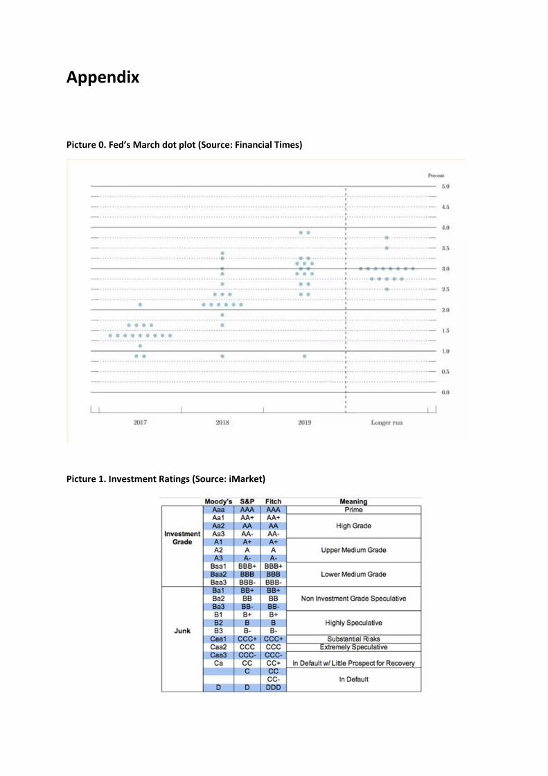
year). If we look at the Fed’s March dot plot (Appendix picture 0), which represents the FOMC’s

projections released along with the policy decision statement, the ‘neutrality’ rate stands between 2.5

and 4 percent (in a 5-year horizon).

As a result of this long-period of zero-interest rate policy, US companies are now 15 to 20 percent

more levered than in 2008 (using net-debt-to-EBITA ratio from Barclays Economics Research) and a

lot of debt is now coming to maturity.

This study reviews the US credit market first, then introduces the Markov-switching model to forecast

corporate defaults using macroeconomic and financial variables (Giesecke et al., 2011), and concludes

by an analysis of the potential solution [or endgame] to counter those rising defaults.

I. Review and analysis of the US credit market

A. Introducing the credit market’s structure

If we look at the capital markets in a general view, they are made up of debt and equity markets, which

purpose is to match the demand for funds with the supply for funds. Global capital markets consist of:

- Primary markets where new securities are issued by governments and companies often

through underwriting.

- Secondary market where the securities issued in the primary markets can be bought or sold.

Most of the activities take place in this sector.

The total US credit market (i.e. debt market) in a broad sense includes bonds and loans. They are both

debt instruments used to finance a particular investment, although there are a few differences. Bonds

are usually issued by companies or governments that want to raise money in order to finance a new

project or meet short term liabilities. Their specificity is that they are tradable in the secondary market.

A loan is defined as a debt obligation between an individual and a creditor; it includes car loans, credit

card loans, mortgages or student loans. They are supposed to be non-tradeable, however through

instruments such as derivatives or securitization they eventually can be traded and liquid.

According to FRED economic data, the total US credit debt (chart 1) – consumer, corporate and

government – reached 64.1 trillion USD as of Q1 2016 (in which there is roughly 40.5 trillions of debt

and the rest of loans), up almost 10tr USD since the last quarter of 2008. For an economy of roughly

18.23 trillion USD, the ratio total-credit-debt-to-GDP stands at 351.7%. In the first quarter of 2016, the

Federal Reserve reported that in its Fed’s Flow of Funds (Z.1) statement and increase of $645 billion

in total credit from the previous quarter. In contrast, nominal GDP increased by ‘just’ USD 65 billion,

which means that it ‘cost’ $10 of new debt to generate a mere $1 in economic growth.

Chart 1. US Total Credit – Debt Securities and Loans (Source: FRED, Q1 2016)

0

10,000

20,000

30,000

40,000

50,000

60,000

70,000

55 60 65 70 75 80 85 90 95 00 05 10 15

Total US Credit

From a risk-based system, debt has systemic consequences compare to equity, therefore the amount

of total equity outstanding in the market should be even bigger. However, as debt is usually cheaper

and increases the cost of capital (i.e. interests on debt are tax deductible), the amount of debt in the

system outperform the amount of outstanding equity by a large number.

Data from the Securities Industry and Financial Markets Association (SIFMA) showed that in the end

of 2015, US bond market represented one-and-a-half time the stock markets with $40 trillion

outstanding (versus $27 trillion dollars for equities respectively), which tells us the importance and

the threat than can impose the bond market.

If we split the US bond market per categories, we get the following:

Outstanding US bonds

Treasury Interest bearing marketable coupon public debt.

Asset-Backed

Includes auto, credit card, home equity, manufacturing, student loans and

other; USD-denominated CDOs are also included.

Money Markets Includes commercial paper, bankers acceptances, and large time deposits.

Mortgage-

Related Product

Includes GNMA, FNMA, and FHLMC mortgage-backed securities and CMOs

and private-label MBS/CMOs.

Corporate Debt Includes all non-convertible debt, MTNs and Yankee bonds, but excludes

CDs and federal agency debt.

Federal Agency

Contains agency debt of Fannie Mae, Freddie Mac, Farmer Mac, FHLB, the

Farm Credit System, and federal budget agencies (e.g., TVA). Beginning

with 2004, Sallie Mae has been excluded due to privatization. Beginning in

2010 Q1, the Federal Reserve Flow of Funds is no longer our source of

agency debt going forward due to FAS 166/167 changes.

Municipal

Due to the change in underlying sourcing from the Federal Reserve,

muncipal securities outstanding has been restated from 2004 onward and

revised upward by about $840 billion.

Sources:

Bloomberg, Dealogic, Thomson Reuters Eikon, Thomson Reuters SDC, U.S.

Treasury, Fannie Mae, Freddie Mac, Ginnie Mae, Farmer Mac, Farm Credit,

FHLB

As you see in the chart below, the main security of the US [public] bond market remains the US

Treasury with $13.9 trillion outstanding (35%), followed by mortgage-related products with $8.9

trillion (23%) and corporate debt with $8.5 trillion (22%).

Chart 2. Outstanding US marketable Bonds (Source: SIFMA)

The SIFMA only reports marketable securities (also called debt held by the public), which is the reason

why the Treasury debt stands far from the 20-trillion USD of US total Federal debt. Marketable

securities consist of bills, Notes, bonds and TIPS; they are negotiable, transferable and can be traded

in the secondary market. Non-marketable securities consist of Domestic, Foreign, REA, SLGS, US

Savings, GAS and Others.

We usually defined Treasuries as credit-risk free as an investment as most credit relationships from

mortgage related products to corporate bonds carry default risk. Then, we have two categories of

investments based on the main three rating agencies – Moody’s, Standard & Poor’s and Fitch

(Appendix – Picture 1):

- Investment grade credit: high grade corporate bond, which is the debt issued by company

with investment-grade credit (BBB and higher credit ratings), riskier than Treasuries. These

companies are usually part of the top S&P500 such as General Electric and pays a slightly

higher yield than the US government.

- Non-investment grade credit or ‘junk’: corporate debt issued by corporate with less than

investment-grade credit (BB or lower), which are subject to a higher interest rate by definition

if they need to borrow

10%

35%

23%

22%

5%2% 3%

US Bond MarketMunicipal

Treasury

Mortgage Related

Corporate Debt

Federal AgencySecurities

Money Markets

Asset-Backed

B. Quick review of the US credit market since the 2008 crisis

1. The Federal Reserve Open Market Operations

As a response to the Great Financial Crisis, the Federal Reserve decreased its target Fed Funds rate

down to zero in December 2008 in order to reinstore stability in the markets and increase the

refinancing activity. Lowering the interest rate usually has a positive impact in the economy as it

lowers the debt service and governments can run large fiscal stimulus for a few fiscal years until the

economy reaches a stable and healthy growth. Between 2009 and 2012, the US government ran four

years of 1-trillion+ USD fiscal deficit in response to the housing market collapse and the global asset

price deflation.

Moreover, the Federal Reserve has also been a major player in the Open Market Operations, i.e.

Quantitative Easing, purchasing outstanding amounts of US Treasuries and mortgage-backed

securities (MBS). The balance sheet (total assets) of the central bank has soared from 1.4 trillion US

dollars in 2012 to 4.48 trillion USD today according to Bloomberg FARBAST index, which could explain

the lift in the equity market (Appendix – Picture 2).

Due to its several rounds of QE (the last one was QE3 and ended on October 28th 2014), the Fed is now

the major holder of US Treasuries with 2.46tr USD (Appendix – Picture 3), far ahead China and Japan

which both cumulate 2.36tr USD of US holdings. The consequence of those series of quantitative

easing is that a tremendous amount of bonds is now coming to maturity within the next 5 years. In

the year 2018 and 2019 alone, there is more than 700bn USD of US bonds maturing and it looks like

the only option the central bank has at the moment is to roll over these bonds and feed the 2025 to

2035 empty years (Appendix – Picture 4).

2. Corporate sector’s response: Buybacks financed by borrowing

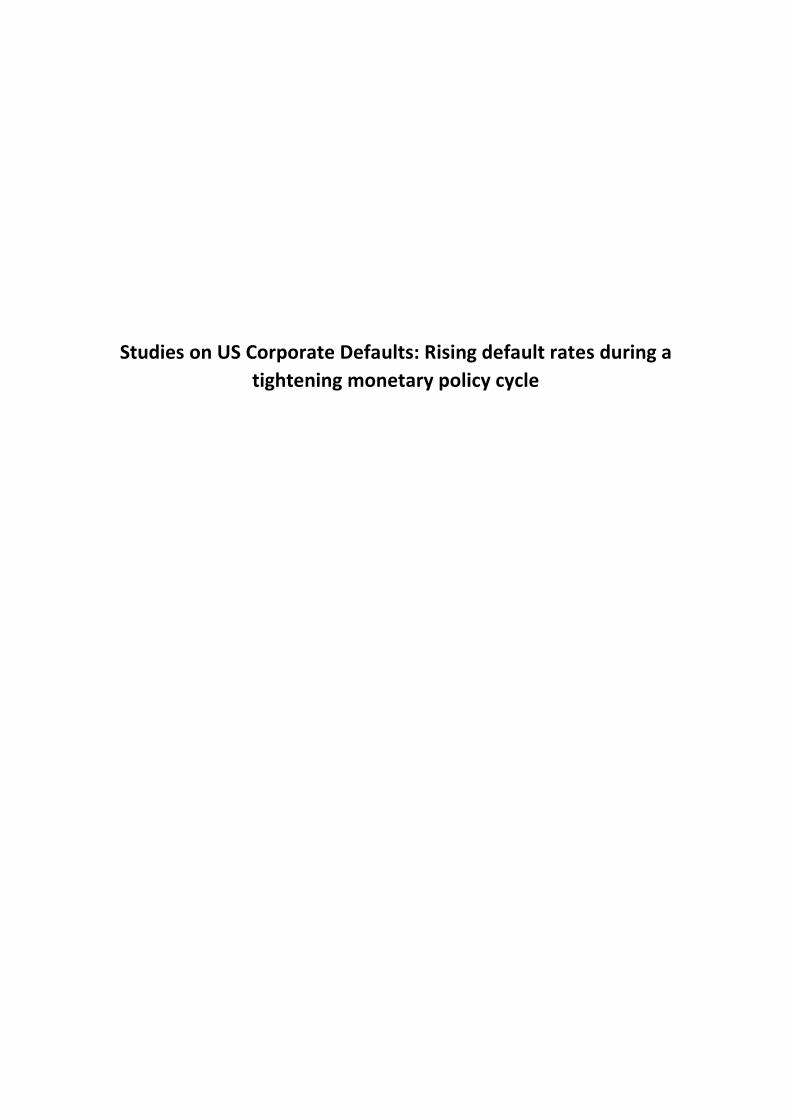
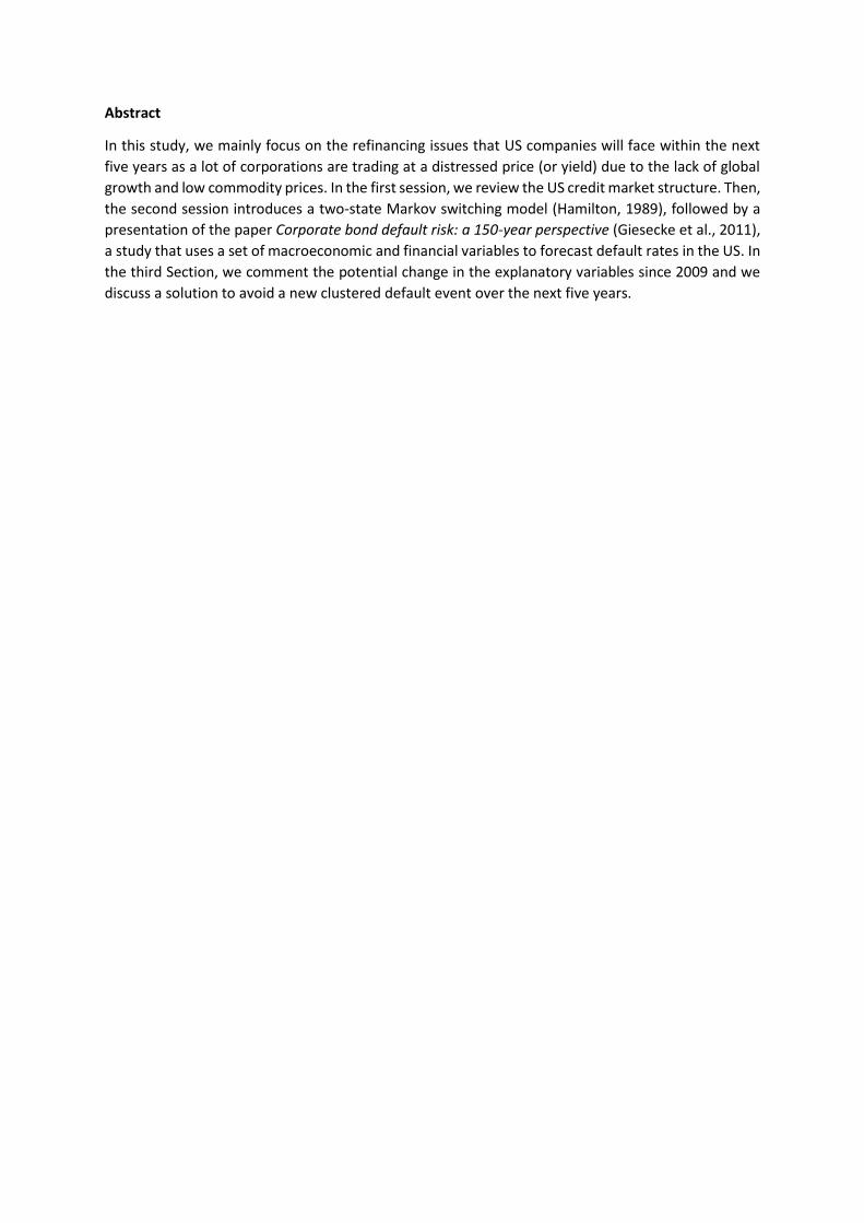
On the corporate side, this long period of zero interest rate policy run by central banks have pushed

companies to finance risky projects (especially in the energy sector) and corporate buybacks. Another

important factor that have explained the equity rally of the past seven years in the US (in addition to

the Fed’s interventions) is that one of the main reasons underpinning demand for US stocks has been

corporate buybacks. It has been described as the ‘sole demand’ for corporate equities, and a study

from Societe Generale Research department has shown that every dollar in buybacks has been funded

by a dollar of new debt (chart 3). With cash flows of both junk and investment grade companies that

have been collapsing for the past 2 years, US non-financial companies are now 15 to 20 percent more

levered than in 2008 if we look at the net-debt-to-EBITDA ratio used by Barclays Research Department.

According to SIFMA, non-financial marketable corporations owed $8.5 trillion in debt in Q1 2016 (a

historical record high), up from $6.6 trillion three years earlier. This rise of the corporate bonds

issuance could be mainly explained by the amount of liquidity in the market in addition to investors’

relentless demand for yield. In a world where more than 10 trillion USD of sovereign and corporate

debt trades in negative territory (as of Q1 2017, down from 13tr USD in August 2016), we can

potentially say that the entire life of the corporate bond market (and especially junk bonds) has been

secularly declining interest rates (one directional move).

Chart 3. Net buybacks and change in debt from US companies and account (Source: Societe

Generale)

We now have a situation where a lot of this debt is about to mature within the next five years, and

major US companies may find difficulties to refinance as their situation has been deteriorating over

the past 24 months. According to S&P’s research (Appendix – Picture 5), there is more than $4.1 trillion

of US Corporate debt slated to mature from now to 2020 included, and a third of that amount is high-

yield. If we look at Picture 5, in the year 2017 and 2018 alone, USD 300 billion junk bonds are maturing;

in the year 2020 alone, there is more than 1 trillion of corporate bond maturing.

As we have the figures in mind, we will now see the issues that the junk bond companies will face in

the future and the potential threat it can create to a ‘fragile’ current market.

C. Issues that the high-yield companies will face

Considering the current ‘fragile’ market, there are four main issues that all these high-yield companies

will face over the next few years:

1. The first one is from poor cash-flow statements: due to this period of low commodity prices,

a lot of companies in the energy space have been running negative cash flow after capital

expenditure, i.e. not covering their dividends or buybacks. With these companies borrowing

money to finance their dividends, corporate finance theory tells us that the riskiness of the

firms start to go up dramatically for the same yield.

2. The second issue is that a lot of investors have been running out of Treasuries to seek higher

yields and positioned themselves in high yield bonds. However, now that the Federal Reserve

is considering starting an interest rate hike over the next few years and raise the target rate

back to ‘neutrality’, we could see a run on these high yield funds. If we look back at the Fed’s

dot plot introduced earlier, policymakers think the Fed Funds rate should be at around 3% –

3.5% in the long term (next 5 years).With an inflation rate close to zero, that would bring a

real return of 3%+ in the short term of the curve, meaning that the investors could potentially

-200,000

-100,000

0

100,000

200,000

300,000

400,000

500,000

600,0000

1/1

2/1

99

0

01

/12

/19

91

01

/12

/19

92

01

/12

/19

93

01

/12

/19

94

01

/12

/19

95

01

/12

/19

96

01

/12

/19

97

01

/12

/19

98

01

/12

/19

99

01

/12

/20

00

01

/12

/20

01

01

/12

/20

02

01

/12

/20

03

01

/12

/20

04

01

/12

/20

05

01

/12

/20

06

01

/12

/20

07

01

/12

/20

08

01

/12

/20

09

01

/12

/20

10

01

/12

/20

11

01

/12

/20

12

01

/12

/20

13

01

/12

/20

14

01

/12

/20

15

Net Buybacks

Change in Debt

get a 5% to 6% real return by investing in LT US Treasuries (10Y, 30Y). This will add further

pressure on these high-yield companies, raising the corporate default risk in the US.

3. The third issue is a consequence of the two first ones and could be more related to behavioural

finance; I call it the ‘deterioration effect’. When a clear bearish trend starts on the high-yield

market due a fast emergence of corporate default, investors and funds will start also to sell

their investments in order to position them on safe-haven asset even if they pay nothing.

Unless the Federal Reserve starts to purchase those bonds until the situation changes, we

could see a sudden run-on-the-high-market. History of the credit market tells us that

corporate defaults happen in clusters (Corporate Bond Default Risk: A 150-year perspective,

NBER). If such a scenario happens, what is going to happen if we see massive ETFs outflows?

We know that usually what stands behind an ETF are bonds that don’t trade; if we see a run

on ETF funds, who is going to guarantee liquidity for these bonds that nobody wants to buy

anymore?

4. The final issue that make the high yield market even more dangerous than the stock market

is that the Volker rule deprives dealers and market makers to hold inventories (limit of 21

business days based on all 2009 customer-to-dealer trades) and has stopped the prop trading

activities run by banks. Therefore, an investor looking to trade a corporate bond would be

either force ‘to hold the asset until a natural counterparty could be identified or transact at

prices that are off market’ (Oliver Wyman, ‘The Volcker Rule restrictions on proprietary

trading’). This situation will definitely decrease the liquidity in the market and especially in

those moments of rapid selloffs.

Now that we introduced the different pockets of the US Bond market, focusing mainly on the amount

of corporate bonds outstanding (high-grade and junk bonds), we will now look at the empirical study

of US history of corporate defaults based on the work of Giesecke et al. (2011).

II. Empirical study of the US Corporate Default history

Firstly, we will introduce the Markov-switching model developed by Hamilton (1989) in addition to a

quick summary of the paper.

A. History of Corporate Defaults (Giesecke & al., 2011) and the regime-switch model

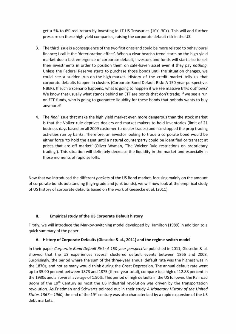
In their paper Corporate Bond Default Risk: A 150-year perspective published in 2011, Giesecke & al.

showed that the US experiences several clustered default events between 1866 and 2008.

Surprisingly, the period where the sum of the three-year annual default rate was the highest was in

the 1870s, and not as many would think during the Great Depression. The annual default rate went

up to 35.90 percent between 1873 and 1875 (three-year total), compare to a high of 12.88 percent in

the 1930s and an overall average of 1.50%. This period of high defaults in the US followed the Railroad

Boom of the 19th Century as most the US industrial revolution was driven by the transportation

revolution. As Friedman and Schwartz pointed out in their study A Monetary History of the United

States 1867 – 1960, the end of the 19th century was also characterized by a rapid expansion of the US

debt markets.

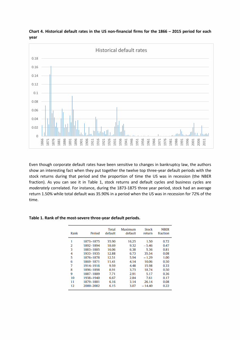
Chart 4. Historical default rates in the US non-financial firms for the 1866 – 2015 period for each

year

Even though corporate default rates have been sensitive to changes in bankruptcy law, the authors

show an interesting fact when they put together the twelve top three-year default periods with the

stock returns during that period and the proportion of time the US was in recession (the NBER

fraction). As you can see it in Table 1, stock returns and default cycles and business cycles are

moderately correlated. For instance, during the 1873-1875 three year period, stock had an average

return 1.50% while total default was 35.90% in a period when the US was in recession for 72% of the

time.

Table 1. Rank of the most-severe three-year default periods.

0

0.02

0.04

0.06

0.08

0.1

0.12

0.14

0.16

0.18

18

66

18

71

18

76

18

81

18

86

18

91

18

96

19

01

19

06

19

11

19

16

19

21

19

26

19

31

19

36

19

41

19

46

19

51

19

56

19

61

19

66

19

71

19

76

19

81

19

86

19

91

19

96

20

01

20

06

20

11

Historical default rates

The authors study if default rates can be forecasted using a set of financial and macroeconomic

variables. As they describe in the paper, there are major changes that have occurred during the 150

years of US corporate bond market in the legal and regulation sides but also in the macroeconomic

atmosphere. Therefore, their approach use a regime-switching framework in studying the

determinants of corporate default risk and introduce a three-state Markov-chain regime-switching

model in which they examine the marginal effects of a vector of financial and macroeconomic

variables in explaining variation in realized default rates. The Markov switching model was first

developed by Hamilton (1989) and is one of the most popular nonlinear time series in the literature.

1. Introduction to regime-switching model (Markov switching model, Hamilton 1989) and the

Bayesian methods

We usually fit stationary time series models, assuming the parameters of the models – the mean and

the variance – remain constant. For instance, we could fit a simple model for a specific financial time

series 𝑦𝑡 (Federal Funds rate, stock market, EURUSD currency). However, history has showed that

there could be a dramatic change in the behaviour of the variable y1t (new monetary policy decisions

or stock collapsing during recession), therefore we could fit several states model and estimates

separate parameters for each state using an indicator variable. Hamilton described this model as ‘a

new approach to the economic analysis of nonstationary time series and the business cycle’. The MS

models can allow for both changes in mean and variance, multiple breaks and can detect outliers in

time series.

Let’s first with a simple MS model with no autoregressive lag and described by the following equation:

𝑦𝑡 = 𝑎𝑆𝑡 + 𝑒𝑡 , 𝑤ℎ𝑒𝑟𝑒 𝑒𝑡~ 𝑁(0, 𝜎2𝑆𝑡)

𝑎𝑆𝑡 = 𝑎0𝑆0𝑡 + 𝑎1𝑆1𝑡

𝜎2𝑆𝑡 = 𝜎2

0𝑆0𝑡 + 𝜎21𝑆1𝑡

In both regime, 𝑦𝑡 follows a normal distribution, though with different means and variances. At each

point in time the, the process St is one out of two regimes, which we indicate by St = 0 and St = 1.

Therefore, the normal probability density function is denoted by the following function f:

𝑓(𝑦; 𝑎, 𝜎2) =1

(2𝜋)0.5𝜎𝑒𝑥𝑝 (−

(𝑦 − 𝑎)2

2𝜎2)

In regime St = 0 and St = 1, we have different distribution as the mean and variance change. Therefore,

we define that St process follows a Markov Chain, meaning that it is a no-memory process and the

probability for regime St = 0 to occur at time t depends solely on the regime at time t-1;

𝑝𝑖𝑗 = 𝑃𝑟[𝑆𝑡 = 𝑖 | 𝑆𝑡−1 = 𝑗]

With,

∑ 𝑝𝑖0

1

𝑖=0

𝑎𝑛𝑑 ∑ 𝑝𝑖1

1

𝑖=0

We have now two free parameters to estimate, which are 𝑝00 and 𝑝11. We will then get the transition

matrix:

p00 p10 p01 p11

where p00 and p11 denote the probability of being in regime zero, given that the system was in regime

zero during the previous period, and the probability of being in regime one, given that the system was

in regime one during the previous period, respectively.

Since the whole processed St is unobserved, we set up the initial regime S1 and introduce another

parameter ξ for the initial probability (i.e. probability that the first regime occurs):

𝜉 = 𝑃𝑟[𝑆1 = 0]

Therefore we have the other scenario:

1 − 𝜉 = 𝑃𝑟[𝑆1 = 1]

We need this extra parameter ξ as there are no conditional information on S0.

As we set the initial values of the vector ε0, we can then compute its values for the next period using

Bayes’ rule, which says that:

𝑃[𝐴 |𝐵] =𝑃[𝐵|𝐴] 𝑃[𝐴]

𝑃[𝐵]

An optimal forecast and inference of the two-state regime need to be made at each t Forr the

inference of the regime at time t=1, this means:

Pr[𝑆1 = 0 | 𝑌1 = 𝑦1] =Pr[𝑌1 = 𝑦1 | 𝑆1 = 0] ∗ Pr[ 𝑆1 = 0]

Pr[𝑌1 = 𝑦1]

Pr[𝑆1 = 0 | 𝑌1 = 𝑦1] =Pr[𝑌1 = 𝑦1 | 𝑆1 = 0] ∗ Pr[ 𝑆1 = 0]

Pr[𝑌1 = 𝑦1|𝑆1 = 0] Pr[ 𝑆1 = 0] + Pr[𝑌1 = 𝑦1|𝑆1 = 0] Pr[ 𝑆1 = 0]

By integrating equation (1) and (2), we eventually get:

Pr[𝑆1 = 0 | 𝑌1 = 𝑦1] =𝑓(𝑦1; 𝑎0, 𝜎0

2) ∗ 𝜉

𝑓(𝑦1; 𝑎0, 𝜎02) ∗ 𝜉 + 𝑓(𝑦1; 𝑎1, 𝜎1

2) ∗ (1 − 𝜉)

Therefore, we can compute the expression Pr[𝑆1 = 1 | 𝑌1 = 𝑦1] = 1 − Pr[𝑆1 = 0 | 𝑌1 = 𝑦1].

Once we computed the inferences for the regimes at time 1, we can use for the time period t = 2,

therefore we have the following:

Pr[𝑆2 = 0 | 𝑌1 = 𝑦1] = Pr[𝑆2 = 0 | 𝑆1 = 0, 𝑌1 = 𝑦1]. Pr[𝑆1 = 0 | 𝑌1 = 𝑦1] +

Pr[𝑆2 = 0 | 𝑆1 = 0, 𝑌1 = 𝑦1]. Pr[𝑆1 = 1 | 𝑌1 = 𝑦1]

As St follows a Markov chain independent of the process Yt, we have:

Pr[𝑆2 = 0 | 𝑌1 = 𝑦1] = Pr[𝑆2 = 0 | 𝑆1 = 0]. Pr[𝑆1 = 0 | 𝑌1 = 𝑦1] +

Pr[𝑆2 = 0 | 𝑆1 = 1]. Pr[𝑆1 = 1 | 𝑌1 = 𝑦1]

We just replace Pr[𝑆2 = 0 | 𝑆1 = 0] and Pr[𝑆2 = 0 | 𝑆1 = 1] by the switching probabilities and we get:

Pr[𝑆2 = 0 | 𝑌1 = 𝑦1] = 𝑝00. Pr[𝑆1 = 0 | 𝑌1 = 𝑦1] + 𝑝11. Pr[𝑆1 = 0 | 𝑌1 = 𝑦1]

We can continue the steps of calculating inference and forecast probabilities for regime 3 and so on,

but we will stop here for the example and construct the series of inference and forecast probabilities

by the recursion:

𝝃𝒕|𝒕 =1

𝝃′𝒕|𝒕−𝟏𝒇𝒕𝝃𝒕|𝒕 ⊙ 𝒇𝒕

𝝃𝒕+𝟏|𝒕 = 𝑷𝝃𝒕|𝒕

where 𝝃𝒕|𝒕 is the vector of inferences probabilities at time t, 𝝃𝒕|𝒕 are the forecast probalities at time t

using the information until time t and ⊙ indicates the element-by-element multiplication.

We then use the maximum likelihood approach to estimate the parameters θ =

{ 𝑎0, 𝜎02, 𝑎0, 𝜎0

2, 𝑝00, 𝑝11, 𝜉} of the regime switching model where the likelihood function will take a

conditional form. By conditioning on the regime at time t, we quickly get the following conditional log

likelihood function:

𝑙(𝑦1, 𝑦2, … , 𝑦𝑇; 𝛉) = ∑(𝝃′𝒕|𝒕−𝟏 𝒇𝒕)

𝑇

𝑡=1

We will use the algorithm of Dempster et al. (1977) to optimize this function, but we won’t develop

the steps as the purpose of this research is to focus and comment the results.

2. Forecasting default rates using a three-state Markov switching model

As we said, fit stationary time series models assume the parameters remain constant. Markov

switching models help us relax this assumption. By allowing different regimes, the regime-switching

model incorporates that the ‘background’ rate of defaults or major structural change (i.e. bankruptcy

law) can occur over time, therefore capturing more complex dynamic patterns. In addition,

macroeconomic environment (i.e. new central banking era) can also change the perspective of

corporate default rates. Let set Dt the default rate for year t, and following Hamilton (2005), we have

the model:

𝐷𝑡 = 𝑎𝑡 + ∑ 𝑏𝑘𝑋𝑘,𝑡−1 + 𝑒𝑡

𝑁

𝑛=1

𝑒𝑡 ~ 𝑁(0, 𝜎2)

Where Xt-1 is a k-vector of ex ante explanatory variables and the bk terms are the corresponding slope

coefficients. The intercept at follows a three-state Markov chain and take values of a1, a2 and a3 with

a transitional probability pi j of moving from state i to j given by the matrix:

p11 p21 p31 p12 p22 p32 p13 p23 p33

By definition, the transition probabilities for the departure states j should add up to one, i.e. p11 + p12 +

p13 = 1. In addition, let set ε it denote the probability (conditional on the data) of being in state i at time

t.

In their study, the vector X is composed of the following explanatory variables:

1. Stock return

2. Stock return volatility

3. Riskless rate

4. Credit spread

5. Consumption growth

6. IP growth

7. Inflation rate

8. GDP growth

In addition, they include the lagged Default rate 𝐷𝑡−1 as default rates tend to depend on previous

default rates time series. This gives N = 9 explanatory variables in total.

Hamilton estimated this model recursively using the maximum estimator method. Let’s define the

parameters of the model in a vector 𝛉 = { 𝑎1, 𝑎2, 𝑎3, 𝑝11, 𝑝12, … , 𝑝33, 𝑏1, … , 𝑏1, 𝜎}.

First, we set the initial values for state probabilities εi0 for i={1,2,3}; then we compute the conditional

likelihood ηjt function as followed:

η𝑗,𝑡 =1

(2π𝜎2)0.5 exp (−

(𝐷𝑡 − 𝑎𝑗𝑡 − ∑ (𝑏𝑘𝑋𝑘,𝑦−1) )2 𝑁

𝑘=1

2𝜎2)

If we sum the i and j the likelihood function ft by:

𝑓𝑡 = ∑.

3

𝑖=1

∑ 𝑝𝑖𝑗

3

𝑗=1

η𝑗,𝑡ε𝑖,𝑡−1

With,

ε𝑗,𝑡 =

∑ (𝑝𝑖𝑗ε𝑖,𝑡−1η𝑗,𝑡)3

𝑖=1

𝑓𝑡

Making the assumption that residuals et are independent and identically distributed, we can then

define the log likelihood function by summing the log likelihoods for each date. The model can then

be estimated using standard maximum likelihood techniques. In their paper, Giesecke & al. set up the

initial values for conditional probability function ε1,𝑖 at one third (i.e. the three states are equally

likely). Then the used an algorithm to maximize the recursively defined log likelihood function.

Summing the log likelihoods for each date, we have the following formula:

log 𝑓(𝑦1, 𝑦2, … , 𝑦𝑇|𝑦0; 𝜃) = ∑ log 𝑓(𝑦𝑡

𝑇

𝑡=1

|𝛺𝑡−1; 𝜃)

for the specific value of 𝜃. An estimate of the value of 𝜃 can then be obtained by maximizing (2) by

numerical optimization. Even though several options are available for the value εi0 , the authors set

the values of ε10 , ε20 and ε30 at 1/3 each and used the Expectation-Maximization (EM) algorithm of

Dempster et al. (1977) for the empirical study.

3. Retracing 150 years of data

The sample consists of 150 annual observations from 1866 to 2015 for the explanatory variables. For

the riskless rate, the authors used the yields on government bonds provided by Homer and Sylla (A

History of Interest Rates, 1991) for the 1866-1989 period and the 10-year Treasury Constant Maturity

Rate from FRED for the 1990 to 2010 period.

For the ‘investment grade’ corporate yields, they also used data provided by Homer and Sylla for the

1866-1989 period, the high-grade railroad bonds for 1866-1899 then the year-end yields for prime

corporate bonds for 1900-1989. Then, they used the Moody’s seasoned Aaa released by FRED for

1990-2010.

The additional four macroeconomic variables were also obtained from different sources. First of all,

the data for inflation rate and consumption growth are both obtained from Chapter Shiller (1989),

available from 1871 (price levels) and 1889 (per capital personal consumption), respectively. Second,

the industrial production data were retrieved from three different sources: from Joseph H. Davis

(2004) for 1865-1915, the index of total physical production for US provided by NBER for 1916-1920

and then the Industrial Production Index from FRED for the 1921-2010 period. Eventually, they used

Simon Kuznets’ work (1961) for the 1885-1929 annual gross national product data and the Bureau of

Economic Analysis for the data on GDP for the 1929-2010 period.

Eventually, for the historical default rates, the authors used four different sources depending the date

range: CFC All bonds (1866-1899), Hick 53 Table A-6 (1900-1943), Atkinson Table 21 (1944-1969), Fed

Flow of Funds – Moody’s (1970-2015).

4. Results interpretation

Table 2 shows the empirical results of the paper. We can see that the three different states are all

statistically significant. In the main state, the constant variable is equal to 0.741%, and the probability

of staying in that environment is close to 90% based on p11 and slightly less than 9% to move up to the

next ‘state of default’. In the second state, the constant variable goes up a bit and stands at 4.2%. In

the final state, we have a constant which is equal to 11.1% and the probability of a ‘clustered’

corporate defaults is increasing sharply under that state.

For the explanatory variables, the first one which is very significant is the default rate at the previous

period, which makes sense as default rate [sort of] follow an autoregressive process. The next period

of default rates tend to highly depend on the situation at the current period. The other variables that

have significant ‘forecast power for subsequent realized default rates’ are the stock returns (negative

sign), the stock market volatility (positive sign) and GDP growth (negative sign). They are all

economically significant as well: the regression results show us that in general, high volatility, negative

returns and lower GDP growth tend to increase the default rates forecasts.

However, two variables that curiously appear to be non-significant are the riskless rate and the credit

spreads, which have a t-statistic of -1.01 and 0.76 respectively. We would have thought that increasing

riskless rates and credit spreads would have definitely a forecast power for realized default rates,

more than GDP growth or stock returns.

Table 2. Results of the MLE of the regime-switching model

In this last section, we will talk about the current situation and comment if the explanatory variables

chosen for the empirical study that we did are still valid in today’s world. We will end with a few

comments on the option(s) we have to avoid another surging clustered defaults in the near future,

and what reaction it may trigger in the market.

III. Interpretations and macro analysis

1. Review of today’s situation in the financial market

As we said in the first part, the Federal Reserve has moved into a zero-interest rate policy (ZIRP) since

December 2008 in response to GFC. In addition, US policymakers announced a series of quantitative

easing measures (QE1, QE2, Operation Twist and QE3) over the past eight years, so that the purchases

of those financial assets (i.e. US Treasuries, MBS) reduces credit spreads, moving investors out of the

risk curve and causing the present value of the assets to go up, which produces the so-called wealth

effect and stimulation. However, academic studies have showed that the effectiveness of monetary

policy tends to decrease in periods of recession or/and when the credit spreads are too narrow.

With the current stock market at all-time high (SP500 Index on its way to hit a record 2,400) and the

volatility trading within its low/scary zone between 10 and 15 (VIX index), the 10-year US Treasury

yields reached a record low of 1.3180% in the beginning of July (July 6th 2016) and has been mainly

trading within a 1-percent range [between 1.5% and 2.5%] over the past year. If we look at the last

two bull markets – the ‘dot com’ market between 1998 and early 2000 and the ‘housing market

bubble’ of 2002 / 2007 – US yields increased from 4.15% to 6.80%, and from 3% to 5.3%, respectively

(Appendix – Picture 6).

In the post-GFC bull market starting mid-2009, US 10-year yields have constantly trended lower, from

a high of 4% to 1.5% while the US equities levitate from 1,100 to 2,160, even though the Federal

Reserve stepped back from the bond market since the last quarter of 2014 (October 28th).

There could be many explanations to that new development (higher equities, but lower sovereign

yields). An intuitive one could be the investors’ constant fear of a sudden reversal in the equity market.

Even though shorting equities sounds easy in theory, market participants are always worried of playing

against the House (government, central bank, the economy…) and therefore tend to increase their

holdings on US Treasuries in order to hedge themselves against a sudden increase in volatility, while

holding their long positions on equities.

An academic candidate [as a response to a decrease in the effectiveness of monetary policy] is

economic uncertainty (Baker et al., 2012). In the working paper Economic Uncertainty and the

Effectiveness of Monetary Policy (June 2013), Aastveit et al. estimated how uncertainty interacts with

the effectiveness of monetary policy, where they concluded that monetary policy is indeed less

effective when uncertainty is high. The authors selected a wide range of uncertainty measures, such

as the US stock market volatility (realized or implied), US corporate-bond spread or time-varying

macroeconomic uncertainty (Jurado et al., 2013).

2. A secular change in the variables of the model

As we described, investors’ fear [or economic uncertainty] could mainly persist in the medium term,

sending nominal US yields to lower levels, while the corporate default rate keeps rising due to low

commodity prices for instance. In this new regime that we entered eight years ago since the start of

central banking interventionism, explanatory variables such as the equity returns or volatility could

become non-significant while corporate spreads and the 10-year riskless rate could have a forecast

power for realized default rates in the future. We think that there should not only be a regime-shift in

the constant, but also in the explanatory variables as well. We believe that the personality of each

variable changes over time, and especially after major macroeconomic structural breaks (i.e. new

central bank regime we entered after the Great Financial Crisis).One interesting exercise would be to

redo the empirical study, using quarterly data but starting in the 1970s (Using S&P and Moody’s data

only).

If we stick with the scenario that the Federal Reserve will increase its benchmark rate up to 4 percent

over the next five years (neutrality rate in the long term according to the Fed’s dot plot), the request

for yields will become much less robust and therefore will add pressure to all the high-yield

investments that market participants have been desperately chasing for the past few years. In that

situation, the economic uncertainty will be transmitted either through choppy market (i.e. higher

volatility), lower US long-term yields as a sort of risk-off environment or a dramatic surge in credit

spread especially in the high-yield market, pushing default rates to the roof.

3. Solutions to counter rising US companies applying for bankruptcy

As rating agency S&P reported, the global corporate defaults just reached 100 and is on its pace to

surpass the 265 total defaults we saw in 2009 within the next two years. That year [2009], the

speculative-grade defaults totalled 223, versus 11 for the investment-grade bonds, pushing the high-

yields default rate to 11.71%.

It is clear that the decline in commodity prices (i.e. the end of the super-cycle) has been a major driver

of all the corporate defaults we have seen over the past 18 to 24 months. Moody’s reported that the

credit quality, mostly in the commodity sector, went down drastically by 70% and 75% in the metals

and mining sector and the energy sector, respectively. Oil prices (WTI front-month roll contract)

declined from a high of $108 per barrel back in mid-June 2014 to reach a low of $26 in mid-February

(i.e. 76% fall from peak to trough) before starting bouncing back to fifty dollars (for a barrel). The first

reason for that fall could be explained by a strengthening US Dollar due to extreme monetary policy

divergence between the US and the rest of the world. Between July 2014 and the beginning of the

second quarter 2015, the US Dollar surged by 25% against the major currencies (we used the Dollar

index for that calculation), its highest increase since the Clinton rally in the mid 90s following the Fed

rate hikes, and sharply impacting the price of oil (and other commodities). The second reason of that

commodity meltdown is due to weakening numbers coming from China. In brief, the Chinese economy

has been constantly showing slower GDP growth figures over the past few years, clearly impacting

global demand for commodities (i.e. thermal coal, iron ore, aluminium, steel and oil) and therefore

international trade. In addition, their currency – the Renminbi – is loosely pegged to the US Dollar (+/-

2% band within the PBoC fixing); so if the US Dollar gets stronger, their currency strengthen as well.

Since early 2011, the trade weighted value of the Chinese Yuan developed by Westpac Strategy Group

increased by 30% (vs. its major trading partners) until August 2015, when the PBoC started its series

of devaluation, impacting drastically Chinese trade balance and commodity prices.

If we look at the change in prices of US High-Yield Corporate Bond ETF developed by Barclays in April

2007 overlaid with Oil prices (Appendix - Picture 7), we can see that they are both highly correlated,

meaning that high-yield companies have been ultimately very sensitive to a change in oil prices. In the

beginning of the year 2016, the average high-yield energy bond was trading at 56 cents on the dollar,

lower than during the financial crisis, sending signals about the outlook for the North American oil

industry. Most of the shale oil companies are now in trouble due to the low price of oil and the

expensive capital expenditure in some part of the US. Ten years ago, the Shale oil revolution

(discoveries of Bakken, Eagle Ford and Green River Foundation) was supposed to be titanic, increasing

the production from 1ml barrels a day to 2ml in 2020 and potentially 3ml barrels per day in 2025

(According to the Energy Information Administration’s 2012 outlook). Experts estimated that 1.2

Trillion barrels of unconventional oil could be extracted from all the different locations in the US,

putting the US as the first oil producer, surpassing Saudi Arabia and its 10-million daily barrels.

According to EIA, the US oil production was averaging 5 million barrels a day in 2005 and has surged

to 9 million today and was supposed to reach 15 million by 2020. With the US consuming 20 million

barrels a day, the lower imports of crude oil based on a higher production would have reduced the

trade deficit and the current account, making the country more sustainable in the long term.

Therefore, in order to provide such a service, a lot of companies in the US have borrowed money to

finance risky projects on an strong assumption that oil will remain ‘strong’ or would never be as weak

as it is today. The EIA estimates that a breakeven price of $72 - $80 per barrel suggested that most

shale oil companies were going to be profitable at a time when oil prices (WTI spot) were trading

above $90/b. According to law firm Haynes and Boone, there were 42 US oil companies that filed

bankruptcy proceedings at the end of June, representing almost $43 billion in cumulative secured and

unsecured debt. The last two important oil & gas companies specialized in exploration that filed for

Chapter 11 bankruptcy protection were SandRidge Energy and Breitburn, which together cumulated

roughly $14 billion of secured and unsecured debt.

Despite the modest recovery in energy prices with oil up 70% compare to its February low, rating

agency S&P and Moody’s estimated that an additional $50 billion of energy debt could default this

year.

The two chart below shows the Moody’s global speculative-grade default counts and rates in global

for each cycle: 1990, 2001, 2009 and the current cycle (based on the report Annual Default Study:

Corporate Default and Recovery Rate, 1920 – 2015 published in Q2 this year). First of all, we can see

the clustered default counts have become more and more important for each cycle. In addition, the

highest corporate default rates for speculative-grade we have seen so far was of 12% in 2009. As of

May 2016 when the report was published, Moody’s forecast of the default rate for the year was 4.2%,

a substantial increase from 1.9% in 2014 and 3.5% in 2015.

0

50

100

150

200

250

300

-3 -2 -1 0 1 2 3

Annual Speculative Grade Corporate Default Counts

1990 2001 2009 Current

4. Conclusion: QE4, the next big move?

We think that if the fragile situation persists in the financial market, the next big move to counter a

drastic increase in default rates would be a new round of quantitative easing in the US, with the

Federal Reserve starting to buy corporate bonds like in the Eurozone or UK more lately. If US

policymakers fail to respond to a default turmoil, a long period of recession could hit the US economy.

Therefore, an potential scenario that may happen is that we could actually seeincreasing rates over

the long-run (5 years) combined with outright purchases of corporate energy bonds during that period

to protect them from applying for bankruptcy.

0.00%

2.00%

4.00%

6.00%

8.00%

10.00%

12.00%

14.00%

-3 -2 -1 0 1 2 3

Annual Speculative Corporate Default Rates

1990 2001 2009 Current

References:

K. Giesecke, F. Longstaff, S. Schaefer, I. Strebulaev, 2011, Corporate Bond Default Risk: A 150-year

perspective

J. Hamilton, 2005, Regime-Switching models

E. Kole, 2010, Regime Switching Models: An Example for a Stock Market Index

M. Friedman, A. Schwartz, 1971, A Monetary History of the United States 1867 – 1960

A. Dempster, N. Laird, D. Rubin, 1977, Maximum Likelihood from incomplete Data via the EM

Algorithm

S. Homer, R. Sylla, 2005, A History of Interest Rates (4th Edition)

K. Aastveit, G. Natvik, S. Sola, 2013, Economic uncertainty and the effectiveness of monetary policy

S. Baker, N. Bloom, J. Davis, 2015, Measuring economic policy uncertainty

K. Jurado, S. Ludvigson. S. NG, 2015¸ Measuring Uncertainty

Moody’s, 2016, Annual Default Study: Corporate Default and Recovery Rate, 1920 – 2015

Appendix

Picture 0. Fed’s March dot plot (Source: Financial Times)

Picture 1. Investment Ratings (Source: iMarket)

Picture 2. Fed’s balance sheet versus S&P500 index (Source: Bloomberg)

Picture 3. Major Holders of US Bonds (Source: Bloomberg)

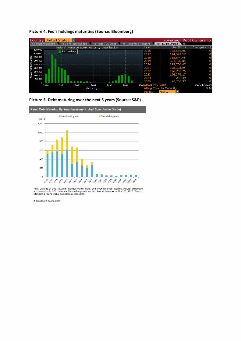
Picture 4. Fed’s holdings maturities (Source: Bloomberg)

Picture 5. Debt maturing over the next 5 years (Source: S&P)

Picture 6. SP500 Index (yellow line) overlaid with the 10-year US Treasury rate (Source: Bloomberg)

Picture 7. WTI prices (candles) overlaid with the JNK index (Green Line)