study and applications of liquid behavior...
TRANSCRIPT

STUDY AND APPLICATIONS OF LIQUID BEHAVIOR ON MICROTEXTURED SOLID
SURFACES
BY
TARUN MALIK
DISSERTATION
Submitted in partial fulfillment of the requirements
for the degree of Doctor of Philosophy in Mechanical Engineering
in the Graduate College of the
University of Illinois at Urbana-Champaign, 2011
Urbana, Illinois
Doctoral Committee:
Assistant Professor Nicholas X. Fang, Chair
Professor Anthony M. Jacobi
Professor Paul J. A. Kenis
Professor Taher A. Saif

ii
ABSTRACT
Engineering the behavior of liquids on solid surfaces has wide applications ranging from the
design of water-repelling surfaces for daily use to fluid flow manipulation in lab on chip devices
and inhibiting corrosion of machinery. Given the ubiquitous interaction of liquids with solids,
these applications only represent a drop in the seemingly endless ocean of opportunities. Thus it
is not surprising that researchers have been trying to decipher this phenomenon for several
centuries now but the complexity of this multi-scale phenomenon has left much to be
understood.
Recent advances in micro/nano manufacturing have granted researchers an unprecedented ability
to control surface texture and properties. This, combined with the fact that surface forces become
increasingly important at small scale, makes it an opportune time to focus studies in the area.
Understanding liquid-solid interaction and developing applications around the same has been a
central theme of this thesis.
In this work, I have explored the solid-liquid interaction at a fundamental level and developed a
thermodynamic model of a liquid drop on a rough surface. The model is validated by several
experimental observations from other researchers. Using the model, I have shown that the
geometry of roughness features could play an important role in the determination of
thermodynamic state of the liquid on the surface as well as characterization of solid surface.
Further, I have used this understanding to predict wetting anisotropy on asymmetric sawtooth
surface and demonstrated the same experimentally.

iii
I also demonstrate a passive cascadable microfluidic logic scheme. The design is centered around
interfacial phenomena and does not require any external power and has no electronic
components. The scheme could replace electronic controls in diagnostic systems leading to
increased portability and reduced costs. It can also be used in environment harmful for silicon
electronics. In another application, geometry based surface patterning is explored in creating wall
less flow in microchannels. I have used the latter to add scalability to the passive cascadable
logic scheme. Wall less flow could also provide tremendous increase in liquid-gas surface area
and open up opportunities to develop liquid-gas reactions systems or possibly „self-cleaning‟ air-
filters.

iv
Dedicated to my wonderful parents
v
ACKNOWLEDGEMENTS
First and foremost I want to thank my advisor Prof. Nicolas X. Fang. I much appreciate his
contribution of time, ideas and funding. He always encouraged me to be independent and
challenged me to hone my ideas. His achievements have always inspired me and I am thankful
for the excellent example he has provided as a successful professor and researcher.
The members of the Fang group have contributed immensely to my personal and professional
time at University of Illinois. I would like to thank: Chunguang Xia, Pratik Chaturvedi, Shu
Zhang, Howon Lee, Anil Kumar, Hyunjin Ma, Keng Hsu, Jun Xu and Matthew Alonso for their
friendship and good advice. Their hard work has always been a source of inspiration.
I would also like to thank my committee members: Prof. Anthony M. Jacobi, Prof. Paul J. A.
Kenis and Prof. Taher A. Saif. They have been very supportive and have always provided me
with much valuable guidance.
I am grateful to the staff of MNMS cleanroom: Bruce Flachsbart, Michael Hansen, Glennys
Mensing and Adam Sawyer. They have helped me immensely and provided much needed
guidance for my work in the cleanroom. I would also like to thank Ankit Raj, Ashutosh Dixit and
Huan Li for help with my experiments and device fabrication.

vi
My special thanks to the staff members of Mechanical Engineering at the University of Illinois,
especially Kathryn Smith. She has been very cooperative and has gone out of her way to help
me.
My time at University of Illinois was made enjoyable in large part due to the many friends who
became a part of my life. They have been my family away from home and have provided me
with support, encouragement and love. I have immensely enjoyed their company and learnt
much from them.
Lastly, I would like to thank my wonderful parents for all their love, encouragement and
sacrifice. I am much thankful to my brother and his wife for keeping me cheerful and always
being supportive. My extended family has always been very encouraging and supported me in all
my pursuits. Special thanks to my loving, encouraging and patient fiancé Neha, whose support
during the final stages of this Ph.D. is so appreciated.

vii
TABLE OF CONTENTS
1. BACKGROUND AND MOTIVATION................................................................................ 1
1.1 Research objective and scope................................................................................................... 1
1.2 Thesis organization…............................................................................................................... 4
2. THERMODYNAMIC MODELING OF ROUGH SURFACES: ROLE OF
ROUGHNESS FEATURES......................................................................................................... 5
2.1 Introduction.............................................................................................................................. 5
2.2 Theory..................................................................................................................................... 10
2.3 „System equilibrium‟ state of the drop.................................................................................... 27
2.4 Comparison with experimental data....................................................................................... 32
2.5 Conclusions............................................................................................................................. 36
2.6 References............................................................................................................................... 37
3. ANISOTROPIC WETTING SURFACES............................................................................ 40
3.1 Introduction............................................................................................................................. 40
3.2 Theory..................................................................................................................................... 41
3.3 Experiments............................................................................................................................ 44
3.4 Comparison of experiment and theory.................................................................................... 50
3.5 Conclusions............................................................................................................................. 51
3.6 References............................................................................................................................... 52
4. PASSIVE CASCADABLE MICROFLUIDIC LOGIC....................................................... 53
4.1 Introduction............................................................................................................................ 53
4.2 Theory and results................................................................................................................... 55

viii
4.3 Passive microfluidic half adder .............................................................................................. 65
4.4 Scalable and cascadable logic scheme.................................................................................... 67
4.5 Methods................................................................................................................................... 70
4.6 Conclusions…......................................................................................................................... 71
4.7 References............................................................................................................................... 72
5. WALL LESS FLOW IN MICROCHANNELS................................................................... 76
5.1 Theory..................................................................................................................................... 77
5.2 Methods................................................................................................................................... 80
5.3 Liquid-wall demonstration...................................................................................................... 81
5.4 „Transfer-channel‟ design....................................................................................................... 82
5.5 Summary................................................................................................................................. 88
5.6 References............................................................................................................................... 88
APPENDIX A: Determination of trapped volume and modified Gibbs Energy Barriers... 90
APPENDIX B: Maximum height and radius of curvature for liquid-wall flow................... 94
AUTHOR’S BIOGRAPHY........................................................................................................ 98

ix

1
1. BACKGROUND AND MOTIVATION
Engineering the behavior of liquids on solid surfaces has wide applications ranging from the
design of „water-repelling‟ surfaces to fluid flow manipulation in lab on chip devices and
designing better surfaces to inhibit corrosion and prevent fouling. Given the ubiquitous
interaction of liquids with solids, these applications only represent a drop in the seemingly
endless ocean of opportunities that understanding the behavior of liquids on solids would
provide. Thus it is not surprising that researchers have been trying to decipher this phenomenon
for several centuries now but the complexity of this multi-scale phenomenon has left much to be
understood.
Recent advances in micro/nano manufacturing have granted researchers an unprecedented ability
to control surface texture and properties. This, combined with the fact that surface forces become
increasingly important at small scale, makes it an opportune time to focus studies in the area.
Understanding liquid-solid interaction and developing applications around the same has been a
central theme of this thesis.
1.1 Research Objective and Scope
The objective of this research is two fold: (1) To develop a theoretical understanding of wetting
on rough/structured surfaces and (2) to use the understanding to develop specific applications -
(a) Anisotropic wetting surfaces (b) Cascadable passive microfluidic logic (c) Wall-less flow in
microchannels

2
The first objective stems from gaining a fundamental understanding, from a thermodynamic
point of view, of the behavior of liquid on rough/structured surfaces. Liquid-solid interactions
are multi-scale, with shaping forces ranging from Van der Walls at the molecular scale to gravity
at the macroscopic level. But recent studies have allowed making reasonable approximations and
a microscopic modeling of the interaction has been shown to be suffice in explaining certain
macroscopic observations. Several researchers have presented such microscopic models in
explaining observations like contact angle, which has been shown to represent one of the several
metastable states that exists for a liquid drop placed on a rough solid surface. Further, it has been
shown that the lowest energy of all such states corresponds to the contact angle determined by
Wenzel relation, called the Wenzel angle, and experimental determination of Wenzel angle can
be used to characterize solid surfaces. However, researchers have neglected the geometry of
surface roughness features in their modeling efforts. In this work the focus has been on
developing a thermodynamic model to qualitatively understand the behavior of a drop on
rough/textured surfaces by accounting for the effect of geometry of roughness features as the
latter could physically limit the states available to the drop and thus modify the associated Gibbs
energy barriers.
Further, several applications are developed based upon the results and insights from the study.
The first application is related to controlling the direction of wettability of a surface based upon
the surface structure. Such surfaces are termed as „anisotropic‟ and can be useful in manipulating
liquid flow with applications in microfluidics.
The second application deals with developing a microfluidics based logic scheme which can be
3
used to integrate control system into lab-on-chip type devices. Although, microfluidic based
logic schemes have been demonstrated in the past but they have either used active devices (like
pumps) or haven‟t been scalable and cascadable. Here, a passive microfluidics based on
interfacial phenomena is explored in designing a scalable and cascadable logic scheme. Such a
system could lead to cheap use-and-throw diagnostic devices and can also be used in
environments which are too harsh for silicon electronics.
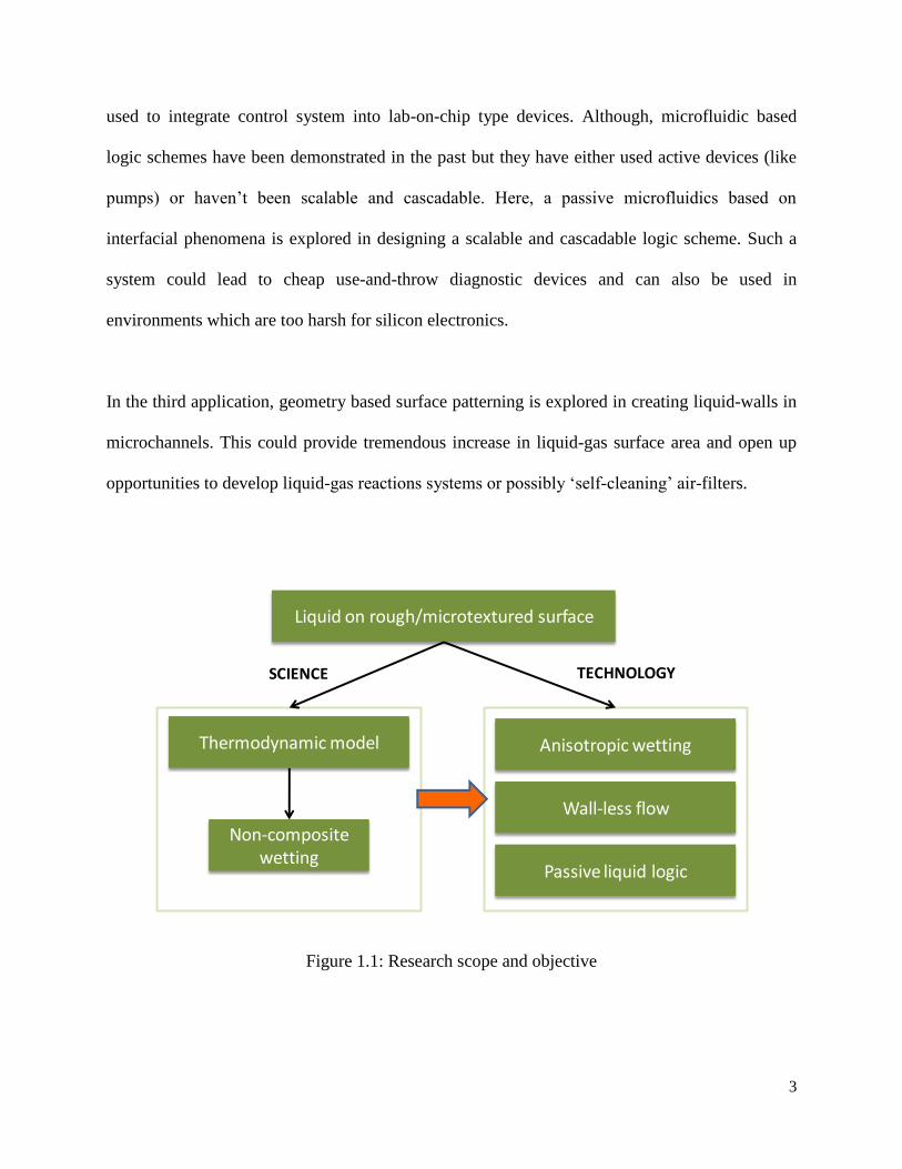
In the third application, geometry based surface patterning is explored in creating liquid-walls in
microchannels. This could provide tremendous increase in liquid-gas surface area and open up
opportunities to develop liquid-gas reactions systems or possibly „self-cleaning‟ air-filters.
Figure 1.1: Research scope and objective
Liquid on rough/microtextured surface
Thermodynamic model Anisotropic wetting
Wall-less flow
Passive liquid logic
SCIENCE TECHNOLOGY
Non-composite wetting

4
1.2 Thesis Organization
This thesis is divided into 5 sections. Following this introduction section is section 2,
“Thermodynamic modeling of rough surfaces: Role of Gibbs energy barriers”. Section 3
presents, “Design of anisotropic surfaces” based on the thermodynamic model in Section 2.
Section 4 details out “Cascadable passive microfluidic logic scheme”. Section 5 entails “Wall-
less flow in microchannels”.

5
2. THERMODYNAMIC MODELING OF ROUGH SURFACES: ROLE OF
ROUGHNESS FEATURES
Assessment of the Young‟s contact angle (YCA) plays an important role in the characterization
of solid surfaces by determination of their surface tension. However, common measurement of
contact angle usually involves measuring a „static‟ contact angle, which is one of the many
metastable states available to the drop. It has been suggested that YCA could be determined by
experimental determination of the global energy minimum of the drop, which has been shown to
correspond to the classical Wenzel angle for „large‟ drops. However, the equivalence of global
energy minimum and Wenzel angle has only be rigorously proven for a drop infinitely larger
than the scale of the roughness, which discounts the geometry of the roughness features and is
not realistic.
Here I present the calculations for a drop, much larger than the scale of roughness, and account
for the effect of geometry of roughness features. It is shown that the latter could physically limit
the states available to the drop. This modifies Gibbs energy barriers and alters global energy
minimum so that the latter may not correspond to the Wenzel angle.
2.1 Introduction
Wetting is the process of making contact between a solid and a liquid [1] in a medium which is
either vapor or another immiscible fluid. It is ubiquitous in nature and has applications in areas
like printing, adhesion, lubrication, painting and many more. Thus, it is not surprising that
6
researchers have been trying to decipher this phenomenon for more than a century now, but
much is left to be understood.
An important and measureable characteristic of wetting systems is the contact angle (CA). It is
defined as the angle between the tangent to the liquid–fluid interface and the tangent to the solid
interface at the contact line of the three phases [2]. It is usually measured on the liquid side.
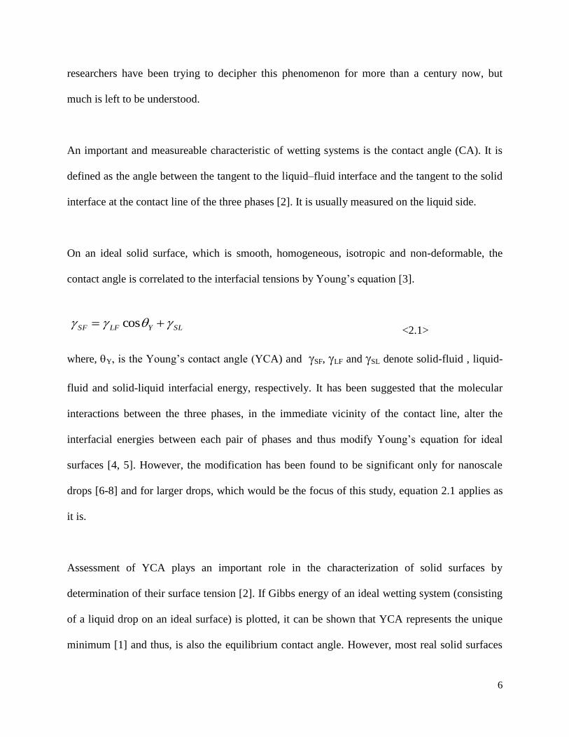
On an ideal solid surface, which is smooth, homogeneous, isotropic and non-deformable, the
contact angle is correlated to the interfacial tensions by Young‟s equation [3].
<2.1>
where, Y, is the Young‟s contact angle (YCA) and SF, LF and SL denote solid-fluid , liquid-
fluid and solid-liquid interfacial energy, respectively. It has been suggested that the molecular
interactions between the three phases, in the immediate vicinity of the contact line, alter the
interfacial energies between each pair of phases and thus modify Young‟s equation for ideal
surfaces [4, 5]. However, the modification has been found to be significant only for nanoscale
drops [6-8] and for larger drops, which would be the focus of this study, equation 2.1 applies as
it is.
Assessment of YCA plays an important role in the characterization of solid surfaces by
determination of their surface tension [2]. If Gibbs energy of an ideal wetting system (consisting
of a liquid drop on an ideal surface) is plotted, it can be shown that YCA represents the unique
minimum [1] and thus, is also the equilibrium contact angle. However, most real solid surfaces
SLYLFSF cos
7
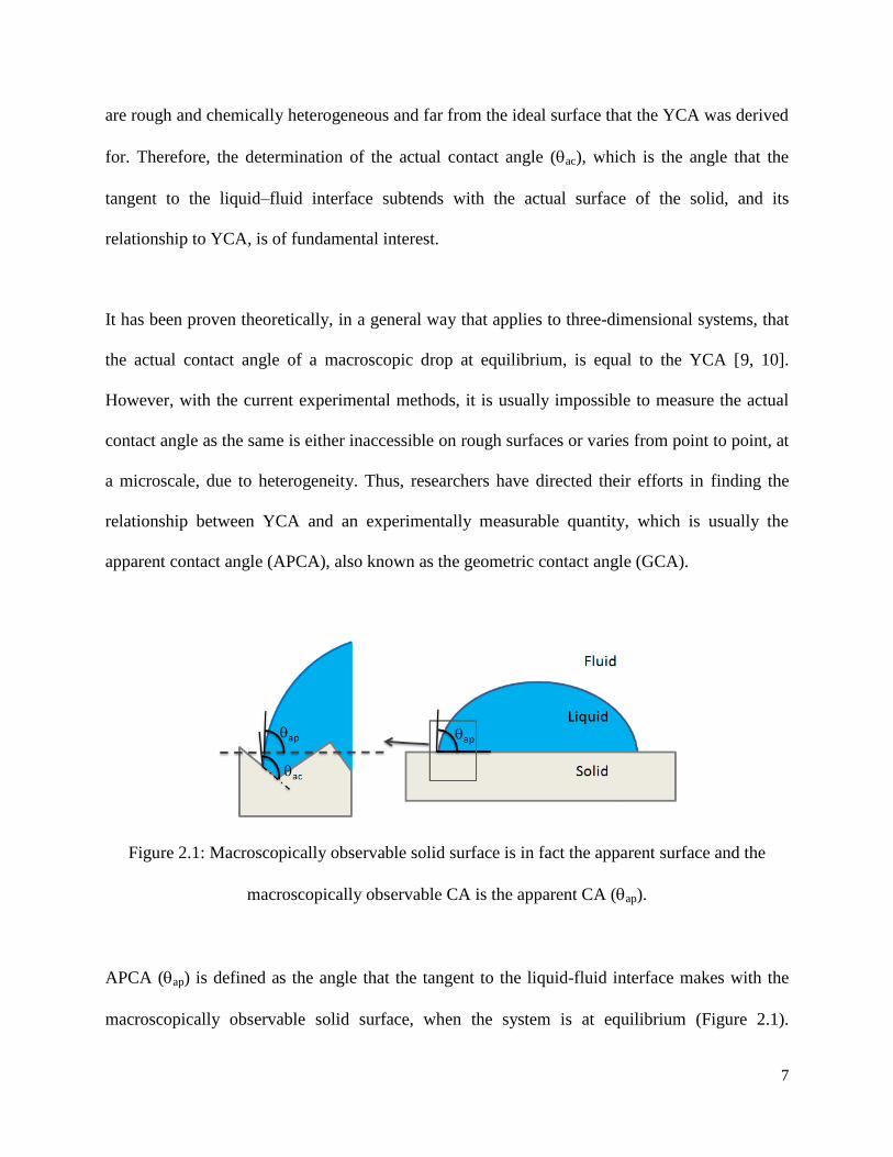
are rough and chemically heterogeneous and far from the ideal surface that the YCA was derived
for. Therefore, the determination of the actual contact angle (ac), which is the angle that the
tangent to the liquid–fluid interface subtends with the actual surface of the solid, and its
relationship to YCA, is of fundamental interest.
It has been proven theoretically, in a general way that applies to three-dimensional systems, that
the actual contact angle of a macroscopic drop at equilibrium, is equal to the YCA [9, 10].
However, with the current experimental methods, it is usually impossible to measure the actual
contact angle as the same is either inaccessible on rough surfaces or varies from point to point, at
a microscale, due to heterogeneity. Thus, researchers have directed their efforts in finding the
relationship between YCA and an experimentally measurable quantity, which is usually the
apparent contact angle (APCA), also known as the geometric contact angle (GCA).
Figure 2.1: Macroscopically observable solid surface is in fact the apparent surface and the
macroscopically observable CA is the apparent CA (ap).
APCA (ap) is defined as the angle that the tangent to the liquid-fluid interface makes with the
macroscopically observable solid surface, when the system is at equilibrium (Figure 2.1).

8
However, it has been found that a range of observable APCAs exist for real surfaces [11-15].
The maximum observable contact angle is called the advancing contact angle, a, and the
minimum is termed the receding contact angle, r. The names are apt as these angles are
observed when contact line just advances or recedes respectively when liquid is added or
removed from a sessile drop. The difference between advancing and receding contact angle is
termed as the contact angle hysteresis (CAH). It is not immediately clear as to how to interpret
the existence of various APCAs and use the information to determine the YCA and thus it
necessary to understand the nature of CAH.
CAH can result due to several factors including surface roughness [13, 14], surface heterogeneity
[12, 15], liquid absorption and/or retention [16-18] and presence of liquid film [19]. Since
roughness and heterogeneity are common characteristics of real surfaces, they have been
investigated most widely. In this paper, the surface is assumed as homogeneous and rough and
heterogeneity would be dealt with in future studies. It is also assumed that the liquid fills in the
roughness grooves of the surface or in other words, the wetting is homogeneous.
Wenzel [20] was the first to describe the effect of surface roughness on surface wettability by
defining a characteristic „Wenzel angle‟, W, for rough surfaces as:
cos(W) = rwenzel*cos(Y) <2.2>
where, rwenzel is the ratio of the actual surface area to the geometrically projected surface area.
The equation was developed based on an intuitive understanding of wetting by averaging out the
details of the rough surface. Shuttleworth and Bailey [13] first pointed out the concept of APCA

9
and provided a quantitative estimate of CAH. Later, Johnson and Dettre‟s seminal paper
provided a thermodynamic perspective of liquid-fluid-solid interaction on rough surfaces [14].
They modeled a two-dimensional drop placed on an axisymmetric sinusoidal surface and
demonstrated the existence of numerous metastable states, which represented different APCAs.
They showed that Gibbs energy barriers exist between different metastable states and argued that
the droplet will assume a metastable state, and the corresponding APCA, based on the available
vibrational energy. Johnson and Dettre also pointed out that when roughness features are small
compared to the drop, the global minimum in Gibbs energy can be approximated by the Wenzel
angle. Several models with additional considerations like gravity [21] and generalized roughness
profiles [22] have been presented since and have corroborated Johnson and Dettre‟s results.
Recently, Wolanski et al. [23] have shown mathematically that for „drops infinitely large
compared with the scale of the roughness,‟ Wenzel angle does indeed correspond to the „global
minimum‟ in Gibbs energy. Although they have not calculated how large the drop should
realistically be, a ratio of two to three orders of magnitude seems sufficient [24].
Thus, it has been suggested that if the global energy minimum is determined experimentally,
YCA can then be calculated using the Wenzel equation. A few methods have been used by
researchers to experimentally determine the global energy minimum, most notably by placing a
drop on a rough surface and subjecting it to vibrations. This allows the drop to overcome Gibbs
energy barriers and reach the „system equilibrium‟ or the „most stable‟ state, which will
correspond to global energy minimum. However, the parameters used to identify the „most stable
state‟ have not been completely and conclusively established. Furthermore, the relation between

10
the „global energy minimum‟ and Wenzel angle has only been rigorously proven for an infinitely
large drop – which is far from a realistic case.
In this study, I present a simplified thermodynamic model of a drop on a rough surface, with the
drop much larger than the scale of roughness. The geometry of the roughness features is
accounted for in the model and it is shown that it physically restricts access to various states that
would have been otherwise available to the drop. The effect of the same on Gibbs energy barriers
and Gibbs energy profile of the system is further explored.
2.2. Theory
Consider a drop sitting on a rough surface with isosceles triangular roughness features. The
particular roughness features have been assumed for ease of calculations and the model
developed henceforth shall apply similarly to other roughness geometries.
The following assumptions are made –
1. Solid surface is non-deformable and chemically homogeneous.
2. Roughness features are infinitely long and extend in direction perpendicular to the paper.
3. Volume of the drop is constant.
4. Drop is long and cylindrical.
5. Drop is „large‟ so that line tension can be ignored [6-8]
6. It is assumed, on physical grounds, that the vertices of the roughness profile are rounded
over a very short distance

11
7. Drop wets the solid in the grooves i.e. wetting regime is non-composite
8. Drop is in thermal equilibrium with the surroundings and there are no external forces.
Chemical reactions are neglected.
9. Dynamic effects due to motion of contact line have been neglected.
10. Adsorbed liquid and liquid-film contribution to contact angle hysteresis are neglected
11. Effect of gravity is negligible
12. Drop is surrounded by air at standard temperature and pressure STP
Using the above assumptions, the drop can be assumed to be two dimensional (2-D). The
schematic of the 2-D wetting system is shown in Figure 2.2. Although a 2-D model is simplistic,
the attempt is here is to illustrate general features of the wetting system. Similar 2-D models
have been previously employed by researchers [14,25-28] and several trends have been validated
by experimental observations. For further discussion on experimental validation, please refer to
section 4.
Figure 2.2: Schematic of two-dimensional drop on a rough surface (x – distance of contact line
from center, P – roughness pitch, – geometric/apparent contact angle for a given x and Adrop)
x
X X’
xs
P
O
Adrop
Ldrop
A C
B
b

12
To model the system, the equation that relates the Gibbs energy of the system to the geometric
contact angle (GCA) of the drop is derived. In Figure 2.2, GCA is the angle that the tangent to
the drop-air interface at X or X‟ subtends with the apparent surface, represented by the horizontal
line XX‟, at a given value of x. It is also referred to as the apparent contact angle (APCA) in
literature.
The Gibbs energy (GE) of the solid-liquid system can be calculated by considering the
contribution of the interfacial energies due to liquid-air (LA), liquid-solid (SL) and the unwetted
solid-air (SA) areas [25] –
<2.3>
For the 2D droplet, the solid-liquid area (ASL) per unit length of the drop is given by the wetted
length of surface roughness features, s –
<2.4>
The liquid-air area (ALA) per unit length of the 2D drop is the perimeter of the drop-air interface,
Ldrop –
<2.5>
With the given assumptions, Young‟s equation is locally valid [6-10] and equation 2.3 can be
simplified to obtain relative Gibbs energy per unit length of the drop:
LALASLSLSASA AAAGE
sin**2
xLdrop
bcos*2
xs

13
<2.6>
Where, LSA is the total area of solid surface (ASA ) per unit length of the surface. Since LSA is
constant for the given problem, it is hereby ignored and the Gibbs energy of the system is
referred to as the „relative‟ Gibbs energy (equation 2.7). Further, to normalize, LA has been
assumed to be 1. It should be noted that equation 2.7 is similar to the equation derived by
Johnson and Dettre [14].
<2.7>
A relation can be obtained between GCA () and x by imposing constant volume constraint. The
volume of the drop per unit length, Adrop (Figure 2.2) is given as:
Adrop = Vol. of OXX‟ – Vol. of roughness features above XX‟ + Vol. of liquid below XX‟
Using simple geometry it can be shown that:
<2.8>
<2.9>
SALAdropYLA LγL*sθγGE *)cos(*
tansin*OXX' of Volume
22xx
2
tan*)2(*2*)1(XX' above features Roughness of Volume
2 bsxN
)cos( dropYrel L*sθGE

14
<2.10>
where, N = x/P rounded off to the lowest integer and xs = (x/P – N)*P
Thus, for a given x, is calculated, which is then substituted in equation 2.6 to calculate the
relative Gibbs energy of the drop. Thereby x is varied and a plot of relative Gibbs energy is
obtained for varying
For this study, the roughness pitch has been assumed as 10 m. Initial GCA and x have been
assumed to be 5 Deg. and 5000 m respectively. This results in a drop volume that corresponds
to a circular 2D droplet with diameter ~ 5.5 mm, which is around 550 times the pitch of
roughness features. The volume of the roughness features is ~3% the volume of the drop.
I model two cases, one with b = 50o and the other with b = 60
o. Young‟s angle is assumed to be
70o. Calculation for Young‟s angle > 90
o are not shown, but will follow in a similar fashion.
2.2.1 CASE I: b = 50o and P = 10 m
With the given roughness parameters, relative Gibbs energy of the drop can be calculated using
equation 2.6 and has been plotted in Figure 2.3.
2
tan*)*2(*2*XX' below liquid of Volume
2 bsxPN

15
The relative Gibbs energy profile initially appears smooth but a close look (inset) shows that it is
sawtooth-like and consists of „valleys‟ and „hills‟. The valleys represent local minimum or
metastable states and correspond to the state when contact line is at the top vertices of the
roughness features, point B in Figure 2.2. The hills represent local maxima or unstable states and
correspond to the state when the contact line is at the bottom vertices of roughness features,
points A or C in Figure 2.2. It should be noted that since the top and bottom vertices are rounded
over a very short distance, they allow the Young‟s contact angle to be locally valid for a given
GCA.
Figure 2.3: Relative Gibbs energy vs. geometric contact angle for triangular roughness profile
with P = 10 m, b = 50o, circular 2D water drop with diameter ~ 5.5 mm, Y = 70
o. Inset:
Zoomed in image
1.00
2.00
3.00
4.00
5.00
6.00
7.00
0 30 60 90 120 150 180
Re
lati
ve G
ibb
s En
erg
y (J
/m X
10-3
)
Geometric Contact Angle
Min. Gibbs Energy (Wenzel Angle)
57.8o

16
The difference in the relative Gibbs energy of a valley (metastable state) and the adjacent hill
(unstable state) is called Gibbs Energy Barrier (GEB) and represents the energy required by the
drop in a given valley to jump to the adjacent valley. If the adjacent valley has a larger GCA,
GEB is termed as GEB - larger GCA (GEB-L) and if the adjacent valley has a smaller GCA,
GEB is called GEB - smaller GCA (GEB-S). This is shown in Figure 2.4, where GEB-L1 and
GEB-S1 are the GEBs associated with state 1.
Figure 2.4: Schematic of Gibbs Energy Barrier
The GCAs corresponding to GEB-L = 0 and GEB-S = 0 represent the maximum advancing and
minimum receding angles, respectively. Metastable states exist only for GCA values between the
maximum advancing and the minimum receding angles. Here, the term maximum and minimum
is applied to advancing and receding angle because they represent the limiting metastable states
in a system with zero perturbation/external noise.
1
2
3
GEB-L1GEB-S1
Re
l. G
ibb
s En
erg
y (J
/m)
Geometric Contact Angle (Deg.)
Hill
Valley
17
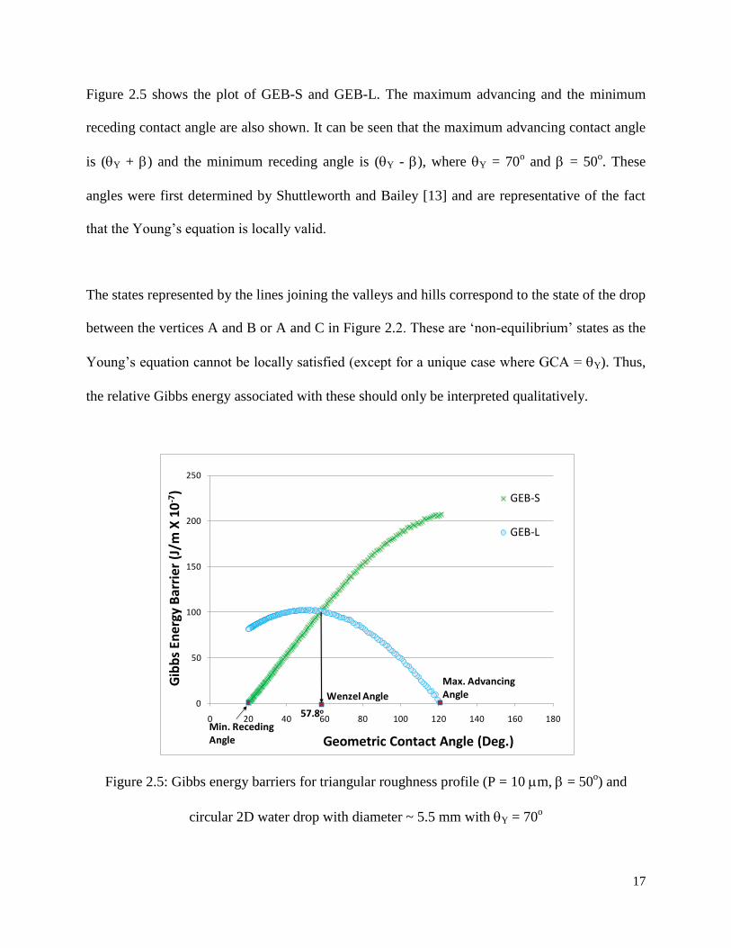
Figure 2.5 shows the plot of GEB-S and GEB-L. The maximum advancing and the minimum
receding contact angle are also shown. It can be seen that the maximum advancing contact angle
is (Y + b) and the minimum receding angle is (Y - b), where Y = 70o and b = 50
o. These
angles were first determined by Shuttleworth and Bailey [13] and are representative of the fact
that the Young‟s equation is locally valid.
The states represented by the lines joining the valleys and hills correspond to the state of the drop
between the vertices A and B or A and C in Figure 2.2. These are „non-equilibrium‟ states as the
Young‟s equation cannot be locally satisfied (except for a unique case where GCA = Y). Thus,
the relative Gibbs energy associated with these should only be interpreted qualitatively.
Figure 2.5: Gibbs energy barriers for triangular roughness profile (P = 10 m, b = 50o) and
circular 2D water drop with diameter ~ 5.5 mm with Y = 70o
0
50
100
150
200
250
0 20 40 60 80 100 120 140 160 180
GEB-S
GEB-L
Geometric Contact Angle (Deg.)
Gib
bs
Ener
gy B
arri
er (
J/m
X 1
0-7
)
Max. Advancing Angle
Min. RecedingAngle
Wenzel Angle
57.8o

18
The GCA with the least Gibbs free energy is shown in Figure 2.3 and 2.5. Although, it is not
possible to mathematically determine the angle corresponding to the global minimum Gibbs
energy for a metastable system [29], it has been suggested that for „large‟ drops, the angle can be
approximated by the classical Wenzel angle [14,23,24]. The approximation seems valid for this
case as the Wenzel angle is W = 57.8o. It is interesting to note that the global energy minimum
is the state where GEB-S is equal to GEB-L. The reasons for the same would be discussed later.
While plotting Figure 2.3 and 2.5, it has been assumed that all the states are available and
accessible to the drop. However, the geometry of roughness features physically restricts access to
certain „unstable‟ states or hills, which correspond to the state of the drop in the bottom vertices
of the roughness features, represented by A and C in Figure 2.2. This modifies Gibbs energy
barriers and alters Gibbs energy profile. To demonstrate the same, two situations are considered
in this study and described as follows:
Case A: > (180 - b
Consider Figure 2.6a where the drop‟s contact line is at B1 or in other words, the drop is in a
metastable state B1. The adjacent hill and valley correspond to the state of drop in vertex C1and
B2 respectively and the energy required to „jump‟ from B1 to B2 is given by GEB-S for state B1:
GEB-S(B1) = GERel,C1 – GERel,B1 <2.11>

19
The terms on right hand side are calculated using equation 2.6.
But as shown in Figure 2.6b, when 1 > (180 - bthe roughness geometry physically restricts the
access to the unstable state at C1. The drop can be assumed to intersect B2 as soon as it reaches
C2, an intermediate point on the roughness profile. Therefore, the geometry of the roughness
features modifies GEB-S of state B1 and the modified value is given as:
GEB-S(B1) MOD = GERel,C2 – GERel,B1 <2.12>
a) b) c)
Figure 2.6: a) Drop with > (180 - b b) Drop „jumps‟ to adjacent peak B2 when >
(180 - b c) Configuration of the drop after the „jump‟
Since, B1 represents local Gibbs energy minimum and C1 represents local Gibbs energy
maxima, therefore the relative Gibbs energy of the intermediate point C2 will lie between the
relative Gibbs energy of C1 and B1 or GERel,C1 > GERel,C2 > GERel,B1. Thus, from equations 2.11
and 2.12:

20
GEB-S(B1) > GEB-S(B1-B2) MOD <2.13>
Hence, for the given roughness profile, when > 130o, the actual GEB-S for state B1 is lower as
compared to the value calculated without accounting for the geometry of the roughness features.
Due to the above reasons, GEB-L of state B2 would also be affected and it is assumed that:
GEB-L (B2) MOD = GERel,B2 – GERel,C2. <2.14>
Again, it can be shown that:
GEB-L (B2) > GEB-L (B2) MOD <2.15>
It should be noted that since the drop is not at equilibrium at C2, the reduction in GEB-L and
GEB-S should be interpreted only qualitatively. For the same reason, Figure 2.6b is just a
representative of one of the several possible configurations of the liquid-air interface. The details
of the calculation can be found in supplementary material.
Case B: < b
Another geometric constraint occurs when the GCA is less than b, so that the corresponding
unstable state is inaccessible to the drop.

21
Consider Figure 2.7, when < b, the unstable state corresponding to the vertex C1 is
inaccessible to the drop and it is assumed that, from an initial metastable state B1, the drop can
jump to B2 as it reaches an intermediate point C2. In this case, GEB-L for state B1 is affected
and it can be shown that the modified Gibbs energy barrier (GEB-L (B1) MOD) is lower than Gibbs
energy barrier calculated without taking the geometric constraint into account. Thus,
GEB-L(B1) > GEB-L(B1) MOD. <2.16>
a) b) c)
Figure 2.7: a) Drop with < bb) Drop „jumps‟ to adjacent peak B2 when < b c)
Configuration of the drop after the „jump‟ with trapped liquid volume
Further, as the drop moves from C2 to the metastable state B2, a small volume of liquid is
trapped in the roughness feature (Figure 2.7c). This liquid volume achieves its own equilibrium
and subtends the Young‟s contact angle with the slanted walls of the shown triangular roughness
feature. The energy and volume of this trapped liquid is taken into account while calculating
Gibbs free energy of the system. Figure 2.8 shows the trapped volume and the change in total
volume of the drop for the case being considered. The details of the calculations for the trapped
volume can be found in the supplementary material.
Trapped volume

22
GEB-S for state B2 is similarly affected and can be calculated as:
GEB-S (B2) MOD = GEB2 – GEC2. <2.17>
As demonstrated earlier, GEB-S (B2) MOD < GEB-S (B2); where GEB-S (B2) = GEB2 – GEC1
Again, the state of drop at C2 is „non-equilibrium‟ and Figure 2.7b is just a representative of one
of the several possible configurations of the liquid-air interface. Thus the reduction in GEB-S
and GEB-L should be interpreted only qualitatively.
A „geometric limit‟ is thus defined as the range of GCAs outside which the Gibbs energy barriers
are modified.
The lower and the upper bound of the geometric limit for the roughness features are given by
band brespectively For the given roughness profile, the geometric limit exists for 50o <
GCA < 130o.
Figure 2.9a shows a plot of relative Gibbs energy for the given roughness profile, both with and
without accounting for the „geometric limit‟. It can be seen that for this case, the global energy
minimum of the wetting system is unaffected and is given by the Wenzel angle.

23
Figure 2.8: Total volume and trapped volume (inset) as a function of GCA for triangular
roughness profile (P = 10 m, b = 50o) and circular 2D water drop with diameter ~ 5.5 mm with
Y = 70o.
Figure 2.9b shows the GEBs. Circles and crosses represent GEB-S and GEB-L calculated
without accounting for the geometric limit. Outside the geometric limit, GEB-S and GEB-L are
modified, as represented by diamond and square respectively. The modified GEBs should be
interpreted only qualitatively. As can be seen, the maximum advancing and the minimum
receding angles are unaffected by the modification of GEBs. It should be noted that GEB-L is
equal to GEB- S at the GCA corresponding to the global energy minimum, given by Wenzel
angle.
14.72
14.74
14.76
14.78
14.8
14.82
14.84
14.86
14.88
0 20 40 60 80 100 120 140 160 180
Geometric Contact Angle (Deg.)
Tota
l dro
p v
olu
me
(m3
X 1
0-7
)

24
(a)
(b)
Figure 2.9: (a) Modified Relative Gibbs Energy and (b) Gibbs energy barriers for triangular
roughness profile (P = 10 m, b = 50o) and circular 2D water drop with diameter ~ 5.5 mm with
Y = 70o. GEBs remain unchanged inside the „geometric limit‟
1.00
2.00
3.00
4.00
5.00
6.00
7.00
0 20 40 60 80 100 120 140 160 180
Rel. GE with Geom. Limit Rel. GE w/o Geom. Limit
Re
lati
ve G
ibb
s En
erg
y (J
/m X
10-3
)
Geometric Limit
Geometric Contact Angle (Deg.)
Min. Gibbs Energy (Wenzel Angle)
Min. Gibbs Energy (with Geom. Limit)
57.8o
0
50
100
150
200
250
0 20 40 60 80 100 120 140 160 180
GEB-S w/o Geom. Limit GEB-L w/o Geom. Limit
GEB-S Modified GEB-L Modified
Geometric Contact Angle (Deg.)
Gib
bs
Ener
gy B
arri
er (
J/m
X 1
0-7
)
Max. Advancing Angle
Min. RecedingAngle
Wenzel Angle
57.8o
Geometric Limit

25
Next, calculations are presented for roughness profile with b = 60o and P = 10m
2.2.2 CASE II: b = 60o and P = 10m
Similar to the analysis for Case I, roughness configuration with b = 60o is modeled. Figure 2.10
shows the total volume of the drop and trapped volume as a function of GCA.
Figure 2.10: Total volume and trapped volume (inset) as a function of GCA for triangular
roughness profile (P = 10 m, b = 60o) and circular 2D water drop with diameter ~ 5.5 mm with
Y = 70o.
14.75
14.8
14.85
14.9
14.95
15
15.05
0 20 40 60 80 100 120 140 160 180
Geometric Contact Angle (Deg.)
Tota
l dro
p v
olu
me
(m3
X 1
0-7
)

26
(a)
(b)
Figure 2.11: (a) Modified Relative Gibbs Energy and (b) Gibbs energy barriers for triangular
roughness profile (P = 10 m, b = 60o) and circular 2D water drop with diameter ~ 5.5 mm with
Y = 70o. GEBs remain unchanged inside the „geometric limit‟
0.50
1.50
2.50
3.50
4.50
5.50
6.50
0 20 40 60 80 100 120 140 160 180
Rel. GE with Geom. Limit Rel. GE w/o Geom. Limit
Re
lati
ve G
ibb
s E
ne
rgy
(J/m
X 1
0-3)
Geometric Limit
Geometric Contact Angle (Deg.)
Min. Gibbs Energy (Wenzel Angle)
Min. Gibbs Energy (with Geom. Limit)
46.8o20.2o
0
50
100
150
200
250
300
0 20 40 60 80 100 120 140 160 180
GEB-S w/o Geom. Limit GEB-L w/o Geom. Limit
GEB-S Modified GEB-L Modified
Geometric Contact Angle (Deg.)
Gib
bs
En
erg
y B
arr
ier
(m X
10
-7)
Max. Advancing Angle
Min. RecedingAngle
Wenzel Angle
46.8o
Geometric Limit
20.2o
Global energy minimum

27
The upper and lower bounds for the „geometric limit‟ are 120o and0
o respectively and the
relative Gibbs energy and GEBs are shown in Figure 2.10. It can be seen that unlike the previous
case, Wenzel angle is not the GCA corresponding to the global energy minimum of the wetting
system. This would be discussed in detail in the next section. The GCAs corresponding to zero
GEBs represent the minimum receding and the maximum advancing contact angle and are 10o
and 120o respectively. As earlier, the maximum advancing contact angle is (Y + b) and the
minimum receding angle is (Y - b), where Y = 70o and b = 60
o.
2.3 ‘System equilibrium’ state of the drop
„System equilibrium‟ state is defined as the state which the system will tend to achieve or, if
moved away, will tend to return to under perturbations which have a Maxwell-Boltzmann
distribution, representative of thermal energy of the molecules at a given temperature. By second
law of thermodynamics, the „system equilibrium‟ state will always correspond to the global
energy minimum. However, for a metastable system, there is no analytical way of determining
the global energy minimum [29]. This section explains as to how the „system equilibrium‟ state
can be determined using Gibbs energy barrier plot and it is shown that modification in the latter
could shift the „system equilibrium‟.
For a wetting system, existence of several metastable states was established by early models and
experiments [14,15, 30-34] and can be seen from the two cases modeled here. At a given
moment, the state in which the drop exists depends on several factors like the method of drop
deposition and the history of the drop. Say, the system in a given state is perturbed and at a given

28
time the magnitude of perturbation is E. Further, assume that the perturbations have a Maxwell-
Boltzmann distribution.
Figure 2.12 shows a section of the relative Gibbs energy profile. Assume that state 3 is the
current state of the system and the corresponding Gibbs energy of the system = GE3. The energy
required to move the system from state 3 is the difference in Gibbs energy of state 3 and an
adjacent „hill‟ – which is either 4 or 2. This difference is given by the GEBs as shown. For
simplicity, it is assumed that GEB-L5 = GEB-L3
Under perturbation E, there could be three scenarios:
Case 1: E < GEB-S3
Case 2: GEB-L3 > E > GEB-S3
Case 3: E > GEB-L3
Figure 2.12: Section of Gibbs Energy profile
3
4
5
GEB-L3GEB-S3
2
1
6GEB-L5
Rel
. Gib
bs
Ener
gy (
J/m
)
Geometric Contact Angle (Deg.)
Hill
Valley

29
In Case 1, the system maintains status quo as it does not have enough energy to reach either state
4 or 2. In Case 2, the system attains state 4 and either comes back to state 3 or goes to state 5. If
the system goes to state 5, it does not have enough energy to come back to state 3 as GEB-L5 >
E and therefore, either the system stays in state 5 or it could move to a state with a smaller
GCA depending on the energy barrier required to do so. In Case 3, the system could either move
to state 4 or state 2 and either return to state 3 or move to state 5 or state 1. If the system moves
to state 5 or state 1, it again has enough energy to return to state 3.
As the perturbations are Gaussian, a perturbation with lower magnitude is more likely a higher
magnitude one. Therefore, since the perturbation required to move to state 5 is smaller than the
one required to move to state 1, it is more likely for the system to move to state 5 as compared to
state 1. For a general case, if Gibbs energy barrier (GEB) required to move to a state with lower
geometric contact angle is less than the GEB required to move to a state with higher geometric
contact angle, over time, the system moves to a state with lower geometric contact angle. A
similar argument will hold if the inverse is true. Thus, to understand the dynamics of the system,
the variation of GEBs for the two cases, modeled here, needs to be understood.
2.3.1 CASE I (b = 50o and P = 10m)
For this case, the following observations can be made from Figure 2.9b:
1. Wenzel Angle lies inside the „geometric limit‟
2. GEB-S = GEB-L at the Wenzel angle

30
To start with, assume that the drop is in a metastable state corresponding to a GCA lower than
Wenzel angle. This state is to the left of the Wenzel angle in Gibbs energy barrier plot (Figure
2.9b) and it can seen that for such a state GEB-L is lower than GEB-S. As explained earlier, over
time, the system would move to a higher GCA and such a movement will continue until the drop
reaches the state where GEB-L is equal to GEB-S, which in this case corresponds to the Wenzel
state. A similar argument would apply when the initial state corresponds to a GCA greater than
the Wenzel angle. Again, the drop would try to attain the Wenzel state where GEB-S is equal to
GEB-L. Further, if the system is moved away from the Wenzel state, in either direction, it will
tend to return back. Thus, for this case, Wenzel state is the „system equilibrium‟ state. Thus, in
this case the modification of GEBs does not play a role in determination of the „system
equilibrium‟ angle.
It can be seen from Figure 2.9a that Wenzel state is also the state corresponding to the global
energy minimum of the system. This is no coincidence but follows from second law of
thermodynamics. It can be shown a perpetual motion machine can be created if the „system
equilibrium‟ state does not correspond to the global energy minimum.
2.3.2 CASE II (b = 60o and P = 10m)
For this case, the following observations can be made from the Figure 2.11 –
1. Wenzel Angle lies outside the „geometric limit‟
2. Due to the modification of GEBs, GEB-S and GEB-L are equal at a GCA different from the
Wenzel Angle.
31
Using similar arguments as earlier, it can be shown that over time, the drop tends to move
towards the state where GEB-L and GEB-S are equal. Due to modification of GEBs, this state is
different from the Wenzel state (Figure 2.11b). Thus, in this case, the „system equilibrium‟ angle
does not correspond to the Wenzel angle.
Also, it can be seen from Figure 2.11a that Wenzel state is not the state corresponding to the
global energy minimum of the system. This state is represents GCA for which GEB-S is equal to
GEB-L and again this follows from second law of thermodynamics. Thus, a generalized set of
condition for isosceles triangular roughness features can be stated as:
If, b < W < 180 - b; then W = „System equilibrium‟ angle
W < b < 180 - b; then W ≠ „System equilibrium‟ angle
b < 180 - b< W ; then W ≠ „System equilibrium‟ angle
Where, slope of triangular roughness feature = bWenzel angle = W.
When Y < 90o, the above relations reduce to: if bW; only then W = „System equilibrium‟
angle. This is plotted in Figure 2.13. Although Young‟s angle can‟t be directly measured, it
represents the hydrophilicity of the surface and is inversely related to the latter. The regime
marked as „complete wetting‟ represents the area where numerically Wenzel angle ≤ 0, since Y
≤ cos-1
(1/r).
It can be seen that for isosceles triangular roughness features, when geometric limit is taken into
account, the range of applicability of Wenzel relation doesn‟t change appreciably unless when

32
roughness features are sharp. However, real surfaces consist of both sharp and blunt three
dimensional roughness features. Such surfaces can‟t be modeled by simply averaging out the
roughness features into a roughness factor, r as geometry could significantly modify the Gibbs
energy barriers and play an important role in determination of „system equilibrium‟. For such
surfaces, it is not immediately apparent as to if the Wenzel angle would correspond to the
„system equilibrium‟ angle (global energy minimum state) and experimental validation is
necessary.
Figure 2.13: Applicability of Wenzel relation for hydrophilic surface with isosceles triangular
roughness features
2.4 Comparison with experimental data
0.00
20.00
40.00
60.00
80.00
100.00
0 10 20 30 40 50 60 70 80 90
Slope of roughness features (Deg.)
Yo
un
g's
con
tact
an
gle
(D
eg.
)
Bluntroughness features
Sharproughness features
Wenzel angle applicable
Complete wetting
33
Several studies [24, 30-34] have attempted the experimental determination of „system
equilibrium‟ contact angle for rough surfaces, yet the same remains an open problem. However,
experiments have helped elucidate some key aspects of the nature of liquid-solid interaction
which allow comparison of the modeling effort and the experimental studies for rough surfaces.
These are presented below -
1. Multiple metastable states: The existence of multiple metastable states of a sessile drop on a
rough surface is very well known [30-33] and supported by the current model.
2. Effect of vibrations on contact angle hysteresis: Experimental studies [31-33] have reported
the reduction of contact angle hysteresis in presence of vibrations. This matches well with the
predictions from the model that vibrational energy allows the drop to overcome Gibbs energy
barriers, thus reducing the advancing angle and increasing the receding angle and thereby
reducing the contact angle hysteresis.
3. Distribution of Gibbs energy barriers: Volpe et al. [32] added vibrations to a standard
Wilhelmy microbalance experiment to obtain a „system equilibrium‟ state of the meniscus on
rough and/or heterogeneous surfaces. They showed that Gibbs energy barriers increase going
toward the absolute Gibbs energy minimum. This result matches with the predictions from the
model for Case I (P = 10m and b = 50o). However, there is still debate over the method used
to experimentally determine the „system equilibrium‟ state. Further, the model presented here
shows that it is not necessary that the Gibbs energy barriers would always increase going to

34
the „system equilibrium‟ state (Case II: P = 10m and b = 60o) and careful experiments are
required to validate the same.
4. Advancing and Receding angles: The values of advancing and receding contact angles match
the predictions by Shuttleworth and Bailey, which have been experimentally shown to be
relevant [34,35].
5. Reproducibility of advancing and receding angles: It has been observed during experiments
[36] on hydrophilic substrates, that receding angle measurements are difficult to reproduce as
compared to advancing angles. This could be attributed to the model‟s prediction that there
are numerous metastable states for contact angles close to receding value while higher contact
angles, close to the advancing value, have fewer metastable states. This can be seen in Figure
2.14.
Figure 2.14: Histogram of metastable states for the same surface as used in Figure 2.11. Each bar
represents the number of metastable states for a GCA range of +/- 5 degrees.
0
10
20
30
40
50
5 15 25 35 45 55 65 75 85 95 105 115 125 135
Nu
mb
er o
f M
etas
tab
le s
tate
s
Average geometric contact angle (Deg.)

35
6. Relation between Wenzel angle and global energy minimum (GEM): Researchers have
suggested measuring the „system equilibrium‟ state of the drop, which will correspond to the
GEM, by placing a drop on a rough surface and subjecting it to vibrations. As the drop
overcomes Gibbs energy barriers, it tries to reach the „system equilibrium‟ state. However, no
conclusive guideline has been established to recognize the „most stable state‟.
Wolanski et al. [37] proved mathematically that when the drop is sufficiently large compared
to the roughness scale, it becomes axisymmetric as it reaches the GEM. Meiron et al. [24]
used the opposite but unproven statement that is: “following vibrations when a large drop on a
rough surface becomes round, it is at the global minimum in energy”, as the working
hypothesis to identify GEM. They measured apparent contact angle on homogeneous surfaces
of varying roughness by vibrating a sessile drop. They used data only from axisymmetric
drops to calculate the contact angle from drop‟s diameter and weight. Their measurements of
„most stable‟ contact angle matched well with the global energy minimum calculations, as
approximated by Wenzel angle, for the rough surfaces. However, the empirical evidence is not
conclusive as the parameters used to identify the „most stable state‟ have not been completely
and conclusively established.
Further, it is shown in this study that since several states are inaccessible to the drop, Gibbs
energy barriers are modified and global energy minimum may not correspond to the Wenzel
angle. However, as pointed out, this shift in „system equilibrium‟ state from the Wenzel state

36
may only occur for surfaces with sharp roughness features and careful experiments are
required to test this conclusion.
2.5 Conclusions
The study presents a two dimensional thermodynamic model for a drop, in a non-composite
state, on a rough hydrophilic surface (Young‟s angle < 90o) with triangular features. Due to the
simplistic nature of model, similar to other two-dimensional models [14,25-28], the attempt is to
illustrate general features of a wetting system.
The model reaffirms the existence of several local equilibrium states for a drop placed on a rough
surface. However, it is pointed out that, due to the geometry of roughness features, the drop is
physically unable to access all the local equilibrium states. This leads to reduction in the Gibbs
energy barriers for the metastable states outside the defined „geometric limit‟. It is further shown
that if the Wenzel angle lies outside the „geometric limit,‟ it will not correspond to the global
energy minimum.
For real surfaces, the result could mean that the Wenzel equation might hold only for surfaces
with weak roughness, where small and blunt roughness features result in a large „geometric
limit‟, or surfaces with weak hydrophilicity, where Wenzel angle is large. For hydrophobic
surfaces, it can be shown that the Wenzel angle might hold only for either weakly hydrophobic
surfaces or surfaces with weak roughness.

37
Although a quantitative estimate of the reduction in Gibbs energy barriers cannot be obtained,
calculations here demonstrate a trend. In cases where Wenzel angle doesn‟t correspond to the
„system equilibrium‟ state, a theoretical determination of global energy minimum is not possible
and the same would have to be measured experimentally. However, such a measurement might
be useless in the estimation of Young‟s contact angle as there may not be any single analytical
equation which could relate the two for surfaces of different roughness.
Supporting Information Available
Appendix A shows the calculation of trapped volume and the modification in Gibbs energy
barriers due to the geometry of roughness features.
2.6 References
1. A. Marmur, Annu. Rev. Mater. Res. 39 (2009) 473.
2. A. Marmur, SoftMatter 2 (2006) 12
3. T. Young, G. Peacock, editor. Miscellaneous works, London‟ J. Murray, Vol. 1, 1855
4. J.W. Gibbs 1961. The Scientific Papers of J. Willard Gibbs, Vol. 1. New York: Dover Publ.
5. A. Marmur, Contact angle and thin film equilibrium. J. Colloid Interface Sci. 148 (1992) 541.
6. A.Marmur, B. Krasovitski, Langmuir 18 (2002) 8919.
7. T. Pompe, A. Fery, S. Herminghaus, J. Adhes. Sci. Technol. 13 (1999) 1155.
8. A.Marmur, J. Colloid Interface Sci. 186 (1997) 462
9. G. Wolansky, A. Marmur, Langmuir 14 (1998) 5292
10. P.S. Swain, R. Lipowsky, Langmuir 14 (1998) 6772

38
11. D. Li., A.W. Neumann. In: A.W. Neumann, J.K. Spelt, editors. Applied surface
thermodynamic. New York‟ Marcel Dekker, Inc.; 1996. Chapter 3.
12. A.W. Neumann, R.J. Good, J. Colloid Interface Sci. 38 (1972) 341.
13. A. R. Shuttleworth, G. L. Bailey, J. Discuss Faraday Soc 3 (1948) 16.
14. R. E. Johnson Jr, R. H. Dettre, Adv. Chem. Ser. 43 (1964) 112.
15. R. E. Johnson Jr, R. H. Dettre, J. Phy Chem. 68 (1964) 1744.
16. C.N.C. Lam, R.H.Y. Ko, L.M.Y. Yu, A. Ng, D. Li, M.L. Hair, A.W. Neumann, J. Colloid
Interface Sci. 243 (2001) 208.
17. C.N.C. Lam, N. Kim, D. Hui, D.Y. Kwok, M.L. Hair, A.W. Neumann, Colloids Surf. A
Physicochem Eng Asp. 189 (2001) 265.
18. C.N.C. Lam, R. Wu, D. Li, M.L. Hair, A.W. Neumann, Adv. Colloid Interface Sci.96 (2002)
169.
19. E. Chibowski, Adv. Colloid Interface Sci.103 (2003)149.
20. R.N. Wenzel, Ind. Eng. Chem. 28 (1936) 988.
21. J. D. Eick, R. J. Good, A. W. Neumann, J. Colloid Interface Sci., 53 (1975) 235.
22. C. Huh, S. G. Mason, J. Colloid Interface Sci. 60 (1977) 11.
23. G. Wolansky, A. Marmur, Colloids Surf. A 156 (1999) 381.
24. T. S. Meiron, A. Marmur, I. S. Saguy, J. Colloid Interface Sci. 274 (2004) 637.
25. A. Marmur, Langmuir, 19 (2003) 8343.
26. A. Marmur, E. Bittoun, Langmuir 25 (2009) 1277.
27. J. Long, M.N. Hyder, R.Y.M. Huang, P. Chen, P., Adv. Colloid Interface Sci., 118 (2005)
173.
28. W. Li, A. Amirfazli, J. Colloid Interface Sci, 292 (2005) 195.

39
29. A. Marmur, Adv. Colloid Interface Sci., 50 (1994) 121.
30. B. T. Lloyd, G. M. Connelly, J. Adhesion, 63 (1997) 141
31. C. D. Volpe, D. Maniglio, M. Morra, S. Siboni, Oil Gas Sci. Technolgy 56 (2001) 9
32. C. D. Volpe, D. Maniglio, M. Morra, S. Siboni, Colloids Surf. A: Physicochem. Eng. Asp.
206 (2002) 47.
33. X. Noblin, A. Buguin, F. Brochard-Wyart, Eur. Phys. J. Special Topics 166 (2009)
34. J.F. Oliver, C. Huh, S.G. Mason, J. Colloid Interface Sci. 59 (1977) 568
35. S. Veeramasuneni, J. Drelich, M.R. Yalamanchili, G. Yamauchi, Polym. Eng. Sci. 36 (1996)
1849
36. H. Y. Erbil, G. McHale, S. M. Rowan, M. I. Newton, Langmuir 15 (1999) 7378
37. G. Wolansky, A. Marmur, Colloids Surf., A 156 (1999) 381.

40
3. ANISOTROPIC WETTING SURFACES
3.1 Introduction
Anisotropic wetting surfaces have special wetting characteristics as they favor wetting in certain
directions more than the others. These surfaces have several possible application e.g. in
microfluidics, preferential drainage in air-conditioning evaporators, evaporation-driven
deposition etc.. Wetting anisotropy has been demonstrated both chemically [1] and using
predefined surface structures [2-6] and the scope of this study is limited the design of anisotropic
surfaces based on the latter.
Several studies have been carried out to design and model anisotropic surfaces based on surface
structure but most of them have been concerned with micro/nano scale parallel grooved
structures [2-6] which provide orthogonal anisotropy - that is the advancing and/or receding
angles are different in directions perpendicular and parallel to the grooves as shown in Figure
3.1.
Figure 3.1: Parallel grooved structures showing orthogonal anisotropy. Insets b) and c) show the
difference in the shape of the drop when it is placed parallel and perpendicular to the grooves
respectively [2]

41
There have been very few studies in left-right anisotropy and those have been mostly limited to
hair/fiber like structures [7]. For a grooved structure, left-right anisotropy implies that the
advancing and/or receding angles depend on the direction of measurement perpendicular to the
grooves. This is shown in Figure 2.2.
Figure 3.2: Left-right anisotropy in bent hair like structures [7]
Based upon the results from the model developed in the earlier section, left-right anisotropic
structures are proposed and characterized in this work.
3.2 Theory
In earlier study, a thermodynamic model was developed for a drop placed on a rough surface.
The roughness was assumed to consist of isosceles triangles. Using the same method, a

42
thermodynamic model is developed for roughness features consisting of asymmetric triangles.
Again, the drop size is „much larger‟ than the size of the drop.
Two surfaces are shown in Figure 3.3 with same geometric features but different orientations.
The assumptions are same as for the model in earlier chapter. The parameters used to model the
surface were - Young‟s contact angle = 70o, b= 20
o, = 70
o, P = 20 m.
(a) (b)
Figure 3.3: Two-dimensional symmetric profiles of sawtooth with asymmetric triangular features
Since, Gibbs energy barriers play a key role in determination of advancing and receding angles,
the same are plotted for both the roughness configurations, as shown in Figure 3.4 a) and b). In
this study, the role of „geometric limit‟ is not considered as it has been shown that the same
would not affect the values of advancing and receding angles here.
As earlier, the maximum advancing and the minimum receding angles in Figure 3.4 correspond
to the maximum and minimum apparent angles as determined by Shuttleworth and Bailey [8].
Also, since Wenzel factor, r [9] is same for both the profiles and hence the Wenzel angle is also
the same (~64o) and corresponds to geometric contact angle with GEB-L = GEB-S.

43
(a)
(b)
Figure 3.4: Gibbs energy barrier vs. geometric contact angle for roughness configuration shown
in inset with P = 20 m, b = 20
o and circular 2D liquid drop with diameter ~1.4 mm
with Y = 70o
0
20
40
60
80
100
120
140
160
0 20 40 60 80 100 120 140 160 180
GEB-S
GEB-L
Max. Advancing Angle
Min. RecedingAngle
Wenzel angle
Geometric Contact Angle (Deg.)
Fre
e En
erg
y B
arri
er
(m X
10^
-7)
Orientation
0
10
20
30
40
50
60
70
80
90
100
0 20 40 60 80 100 120 140 160 180
GEB-S
GEB-L
Max. Advancing Angle
Min. RecedingAngle Wenzel angle
Geometric Contact Angle (Deg.)
Gib
bs
Ener
gy B
arri
er (
J/m
X 1
0^-7
)
Orientation

44
However, it is interesting to note the two surfaces have different advancing and receding angles.
This result is used in the design of anisotropic surfaces in the next section.
3.3 Experiments
Simulations in the previous section demonstrated the difference in the advancing and receding
angles of two similar roughness profiles with different orientations. Based upon the simulations,
it is proposed that surface with an asymmetric periodic sawtooth profile would demonstrate
anisotropy and the advancing and receding angles would depend upon the direction in which
measurements are taken along the sawtooth.
Figure 3.5a shows the surface profile of an Echelle grating (GE1325-0875) having 79
grooves/mm and a blaze angle of 75o that was purchased from THOR labs (www.thorlabs.com).
The surface of the grating is coated with Alumina and has the desired asymmetric periodic
sawtooth profile. As shown in the figure, a nomenclature of +ve and –ve is assumed to denote
the orientation of sawtooth.
(a)
Figure 3.5: Continued on next page
+X
-X

45
(b)
Figure 3.5: (a) Schematic of Echelle grating GE1325-0875 with 79 grooves/mm. Direction of
arrow indicates orientation of sawtooth, +x and –x represent the head and tail of the arrow
respectively (b) SEM image of the grating
Contact angle measurements were made using a Contact Angle System OCA 20 (DataPhysics
Instruments GmbH, Germany) at 18.8 C and 40% RH. The usual contact angle variability for the
measurement technique used is +/- 2°.
3.3.1 Measuring wetting anisotropy
A common method to measure the wettability of a solid surface for a given liquid is to determine
the static contact angle. Researchers have used difference in static contact angle as a measure of
anisotropy, specially so in the case of orthogonal anisotropy [2, 6]. However, it was shown in the
earlier chapter that static contact angle of a liquid on a rough solid surface represents one of the
several metastable states that the drop can exist in. Hence, static contact angle is not a good

46
measure of anisotropy as it is not repeatable and depends on method of drop deposition and thus
should only be used as a qualitative measure of anisotropy.
Tilt angle required for sliding of drops deposited on a surface have also been used to measure
anisotropy [4]. However, the critical tilt angle of a drop depends on the advancing and receding
angle and the shape of contact line. The latter could be difficult to reproduce in different
experiments and thus doesn‟t provide a repeatable method of measuring anisotropy.
In this study, advancing and receding contact angle measurements have been used to measure
left-right anisotropy. The measurements have been shown to be repeatable using two different
experimental methods.
3.3.2 Static contact angle measurements
As pointed out earlier, static angle measurements should only be used as a qualitative
measurement of anisotropy. Here, static contact angles are measured by depositing a 3l drop
from different heights on to the surface of the grating. The measurement data is shown in Figure
Figure 3.6 (a) and (b) for the parallel and perpendicular directions with respect to the sawtooth
profile respectively. The different contact angles in Figure 3.6 are representative of different
metastable states that the drop assumed as it was let go from different heights.

47
(a)
(b)
Figure 3.6: Contact angle data (a) parallel and (b) perpendicular to the sawtooth
Although, the contact angle data above doesn‟t show any significant anisotropy, the same is
apparent when liquid is added and removed from the droplet.
As shown in Figure 3.7a, as liquid is added to the droplet, the contact line advances in only one
direction and the droplet becomes asymmetric with respect to the fixed red colored reference
line. Also, as the liquid is removed from the droplet, Figure 3.7b, the contact line starts receding
from one end, which is different from the end where the contact line was advancing.

48
(a)
(b)
Figure 3.7: Wetting anisotropy apparent in unidirectional advance of contact line with (a)
addition and (b) removal of water
3.3.3 Advancing and receding contact angle measurements
Due to wetting anisotropy, the measurement of advancing and receding contact angles was not
possible in the usual manner - that is by addition and removal of liquid from the drop, as the
liquid would advance and recede from only one end. Thus, two different methods were used and
compared for repeatability.
A) Constant drop volume, varying tilt stage angle

49
In this method, the drop volume was fixed at 30 l and the tilt stage angle was varied until the
drop just started to slide and the advancing and receding angles were measured. This experiment
was only done for the orientation of sawtooth shown in Figure 3.8. The measured advancing and
receding angles were 89o and 25
o respectively. This is shown in Figure 3.8, for the given
orientation of the sawtooth.
Figure 3.8: Measurement of advancing and receding angle using fixed drop volume method.
Orientation of sawtooth shown in the images. Advancing angle = 87o, Receding angle = 25
o
B) Varying drop volume, constant tilt stage angle
In the second experiment, the tilt angle of the stage was fixed and water was added to the droplet
until the contact line started to move. This gave an advancing angle of 130o and 85
o for drop
sliding towards the +ve and the –ve direction respectively. The latter reading matches well with
the data from fixed drop volume, varying tilt angle experiment.
Drop
Grating
Tilt stage

50
(a) (b)
Figure 3.9: Measurement of advancing angle with fixed tilt angle method. Orientation of
sawtooth is shown in the images
3.4 Comparison of experiment and theory
Table 3.1 compares the advancing and receding angle measurements from the experiments and
the predicted value based upon Shuttleworth and Bailey equation [8]. It should be noted that the
predictions are the theoretical maximum values for the advancing and recessing angles as the
vibrations haven‟t been taken into account. The Young‟s contact angle assumed for Alumina is
65o.
As can be seen, the advancing angle measurements match well with the predictions. The model
overestimates the receding angle measured along the direction of the arrow as shown in Figure
3.5a. This error could be due to the presence of liquid film on the surface [10].
~130 Deg ~85 Deg

51
Table 3.1: Comparison of experimental data and predictions for sawtooth profile based on [8].
Experimental error = +/- 2 Deg.
3.5 Conclusions
Thermodynamic model was developed for two asymmetric triangular roughness profiles with
different orientations. The model predicted the same Wenzel angle but very different advancing
and receding angles for the two profiles. This result was used to predict left-right anisotropic
surface geometry which was characterized using an off-the-shelf optical grating. It was found
that although the static contact angle measurements showed only minor anisotropy, the
advancing and receding angle measurements revealed the wetting ratchet like characteristics of
the surface. These surfaces pave the way to design smart surfaces to manipulate and control
liquid motion on the same.
Direction of measurement
PredictionData
(Average of 3)
Drop movingalong arrow
Advancing 140o 128o
Receding 45o 25o
Drop movingagainst arrow
Advancing 80o 85o
Receding 0o TBD

52
3.6 References
1. B. Zhao, J.S. Moore, D.J. Beebe, Science, 291 (2001) 1023.
2. D. Xia, S.R.J. Brueck, Nano Lett., 8 (2008) 2819.
3. W. Li, G. Fang, Y. Li, G. Qiao, J. Phys. Chem. B 112 (2008) 7234.
4. A. Sommers, UIUC, PhD Thesis, 2007.
5. J.Y. Chung, J.P. Youngblood, C.M. Stafford, J.Y. Chung, Soft Matter 3 (2007) 1163.
6. Yan Zhao, Qinghua Lu, Mei Li, Xin Li, Langmuir 23 (2007) 6212.
7. Kuang-Han Chu, Rong Xiao, Evelyn N. Wang, Nature Materials 9 (2010) 413
8. A. R. Shuttleworth, G. L. Bailey, J. Discuss Faraday Soc 3 (1948) 16
9. R.N. Wenzel, Ind. Eng. Chem. 28 (1936) 988
10. N. Patankar, Langmuir, 19 (2003) 1249.

53
4. PASSIVE CASCADABLE MICROFLUIDIC LOGIC
Surface tension based passive pumping and valving is used to design a fully cascadable
microfluidic logic scheme. Using the scheme, a microfluidic equivalent of a half adder is
demonstrated. Such a scheme can be used as a cheap replacement for electronic controls in
microfluidic based systems e.g cheap use-and-throw diagnostic devices. They could also
have applications in environments harmful to electronic controls and in space/low gravity
environment.
4.1 Introduction
Microfluidic diagnostics has advanced much in the recent years with many interesting
applications being explored by researchers [1-5]. However, its impact on developing countries is
yet to be seen in a big way. As pointed out by Yager et al. [6], part of the reason is the fact that
these devices were designed for air-conditioned labs with stable supply of power and trained
personnel, which the developing countries lack. Further, portability, and low cost, amongst
others, are essential design requirements for markets in the developing world which the current
diagnostic systems lack.
As interfacial forces become significant at microscale, low power requirement can be
obtained in microfluidic systems enabled by capillary forces. Further, since incorporation of
active devices necessitate requirement of additional equipment, capillary enabled systems
can offer cost savings and portability. Thus, capillary-based passive devices are very
attractive candidates for design of cheap diagnostic systems.

54
Researchers have demonstrated capillary driven pumping schemes [7], microdispenser [8],
self-fluid replacement mechanisms [9]. Further, surface and geometry modulation have
enabled the design of passive microfluidic valves [10-13]. A detailed review of various passive
microfluidic schemes can be found elsewhere [14]. Inspite of all these advancements, the
controls for microfluidics have essentially remained electronic or pneumatic. Thus, for
portability, lower cost and ease of usage, it would be desirable to integrate controls into a
diagnostic microfluidic platform.
Fluid based logical devices were developed in 1950‟s [15] but lost to electronics as the latter
scaled down in size and increased in speed. These earlier fluidic devices took advantage of
the turbulent flow which is not accessible at smaller scale as the viscous forces dominate.
Therefore, a completely different approach is required to design control elements for
microfluidic systems.
Several researchers have attempted to design logical elements using microfluidic systems.
Vestad et al. [16] demonstrated microfluidic on-chip logic operations (And, Or, Xor, Nand and
Not) by using laminar flow to achieve a nonlinear system functional response. However, their
device could not be cascaded as it used two different fluids streams. Using immiscible liquids,
Prakash et. al [17] invented „bubble logic‟ and demonstrated universal Boolean logic, bistability
and numerous other traits associated with a scalable logic family. In other works, multiphase
flow [18], pneumatics [19] and chemical reactions [20] have been used to demonstrate
microfluidic logic and memory elements. However the systems either required active elements
or could not be cascaded.

55
Passive liquid-liquid triggered valve which acts as an AND gate has been successfully
demonstrated [10-13, 21, 22], but it lacks the functionality required for a complete control
system. Passive droplet based logic devices have been designed by Toepke et al.[23] and
although the design can be cascaded, an external pipeting system is required for automation
which compromises portability. Thus, the development of a cascadable passive microfluidic
logic is required which can be easily scaled
In this work, a scalable design scheme for passive cascadable microfluidic logic is proposed
and a passive microfluidic half adder is demonstrated.
4.2 Theory and Results
A sudden expansion in flow cross-section can stop a liquid stream driven by interfacial
forces [10-13, 21, 22]. Using the same basic principle, a channel geometry shown in Figure 4.1
is modeled and studied. For sake of simplicity, the channel is designed so that inputs A and B are
geometrically similar. Liquid is introduced into one of the inlet channels and is driven by
capillary force to the channel junction, where it encounters a sudden expansion in cross-sectional
area. Based on the channel geometry and dimensions, the liquid either stops or jumps the
junction to flow to the outlet. If the liquid happens to stop and liquid is introduced into the other
input channel too, the meniscus meet at the junction and again, depending on channel
dimensions, liquid can either stop or jumps the junction to reach the outlet. The possibilities are
summarized in the Truth Table in Figure 4.1 and represent various logic gates i.e. AND [10-13,

56
21, 22], OR and STOP valve. The 0s and 1s, in the Figure, represent the presence and absence of
liquid in a given Inlet/Outlet.
Figure 4.1: Schematic of channel geometry and the truth table for different possible output
scenarios (W – Width of inlet channels, H – Depth of the device: not shown, b – geometric
expansion angle)
4.2.1 AND and OR gates
For a static liquid-meniscus stopped at a sudden expansion shown in Figure 4.1, the pressure
required to break the same can be calculated using the Young‟s equation [24] –
Where, a is the advancing contact angle of liquid on substrate and the maximum value of
(a) and (a) is . The latter condition ensures correct calculation of the maximum break
pressure. The second term on the left hand side of the equation accounts for the maximum
1
2
b1
BA
OUT
Truth Table
)*/()]cos(**2)cos(* )cos(*[** 21 HWWHHHgP aaaA

57
pressure on the meniscus due to the weight of the liquid. This contribution can be neglected for
channels smaller than capillary length, lo = sqrt(/g), which is ~2 mm for water at 25oC, 50%
RH with g = 9.8m/s2. Since the dimensions of liquid channels in this study are smaller than the
capillary length, gravity term is neglected. Also, it is assumed that no other body force (e.g.
magnetic) is acting on the meniscus. Non-dimensionalizing the above equation gives -
<4.1>
Equation 1 represents the non-dimensionalized break pressure for a single channel. However, if
the liquid is present in both the channels – A and B, the break pressure can be calculated as –
In the above equation, b1 is that expansion angle that the liquid meniscus is subjected to after
streams from inlets A and B combine. As explained earlier, max.[(ab)]=. Again, it is
assumed that no other body force acts on the system. Non-dimensionalizing the equation and
neglecting gravity (system assumed to smaller than capillary length) -
<4.2>
)]cos(*)/()cos()[cos(
/)*(""
21
dim_
aaa
AAnon
HW
WPPAINLETDP
)*/()]cos(**2 )cos(**2[** 1 HWWHHgP aaBA b
)]cos(*)/(*2)cos(*2[
/)*(""
1
dim_
aa
BABAnon
HW
WPPBAINLETDP
b

58
Figure 4.2 shows the plot of break pressure for single and two channels for varying W/H. If the
break pressure is positive, the liquid in the channel is not stopped by the sudden expansion and
flows to the outlet and vice versa.
Three regimes of operation can be chalked out from Figure 4.2. For the first regime, the
break pressure is negative for both single and combined channels. Thus the liquid can‟t pass
the sudden expansion junction and the same acts as a STOP valve. It is easy to see that the
STOP valve can function as a microfluidic diode, since it would allow liquid to flow through
if the liquid approached the junction from the side labeled as OUT but not when the liquid
approached the junction from channels A and/or B.
In the second regime, the break pressure is negative when the liquid is present in a single
channel but it is positive when the liquid is present in both the channels. Thus the system acts
as an AND Gate (Figure 4.1). In the third regime, the sudden expansion is not able to stop
the liquid and the system acts as a OR Gate (Figure 4.1).

59
Figure 4.2 Break pressure for varying W/H (W=500m, A=78o1=110
o, 2=140
o, b1= 90
o,
= 0.072 N/m)
From Figure 4.2, it can be concluded that the channel junction, shown in Figure 4.1, can function
as both AND and OR gate depending on the device depth or channel width. For ease of
manufacturing and to realize a cascadable system design, it is desired that the device depth of
AND gate and OR gate be the same. Thus, OR gate is designed as shown in Figure 4.3, wherein
each input ANDs onto itself thereby allowing liquid to reach output when any or both the
channels contain liquid (or any or both the inputs are 1).
-2
-1.5
-1
-0.5
0
0.5
1
1.5
0 1 2 3 4 5 6
DP-INLET-A
DP-INLET-A-B
No
n-d
ime
nsi
on
alP
ress
ure
W/H
AND GATE
STOP VALVE
OR GATE

60
Figure 4.3 Alternative scheme for OR gate wherein each input ANDs onto itself
Figure 4.4 shows the operation of AND gate. PMMA was used as the device substrate, since it is
naturally hydrophilic (A = 78o), and the liquid was de-ionized water colored with red food dye.
The width of input channels was 500 m, the depth of the device was 300 m and the expansion
angles (1 2) at the junction were 150o. With these dimensions, the calculated break pressure
of a single channel was -188 Pa and -44 Pa for both the channels. Here, the break pressure for
both the channels in negative, contrary to what is shown in Figure 4.2. However, the drop placed
at the inlet has a net positive pressure of around 100 Pa, which counters this negative pressure
and allows for AND gate functioning. As can be seen from the figure, water is allowed to the
outlet only when both the channels have water present (both the inputs are 1).
Figure 4.5 shows operation of OR Gate. The parameters and materials used in the design of OR
gate were the same as the AND gate and the calculated break pressure for single input, which
ANDs onto itself, was –44 Pa. This negative pressure was again countered by the positive
pressure due to the drop present at the inlet. As can be seen, the water moves to the output once it
is introduced in one of the inputs.
Inlet A Inlet B
Out
AND
Gate
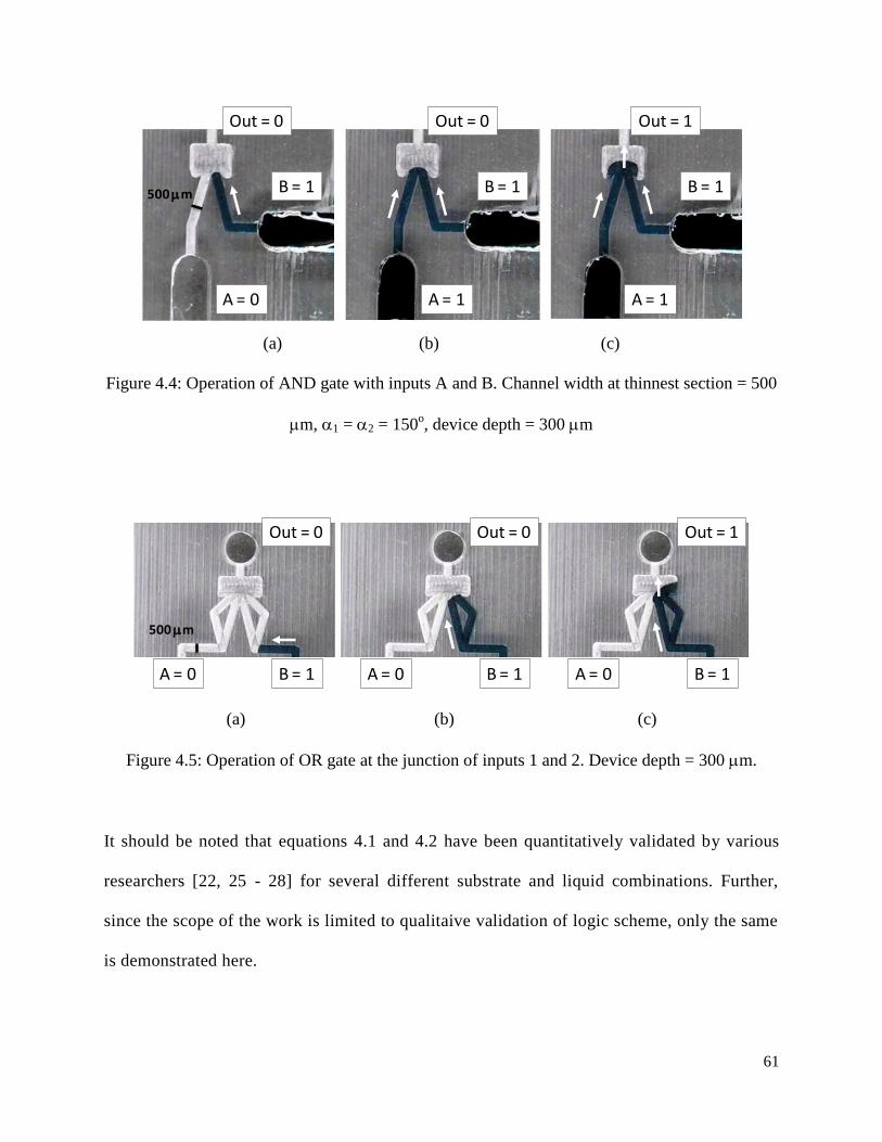
61
(a) (b) (c)
Figure 4.4: Operation of AND gate with inputs A and B. Channel width at thinnest section = 500
m, 1 = 2 = 150o, device depth = 300 m
(a) (b) (c)
Figure 4.5: Operation of OR gate at the junction of inputs 1 and 2. Device depth = 300 m.
It should be noted that equations 4.1 and 4.2 have been quantitatively validated by various
researchers [22, 25 - 28] for several different substrate and liquid combinations. Further,
since the scope of the work is limited to qualitaive validation of logic scheme, only the same
is demonstrated here.
B = 1
A = 0
Out = 0
B = 1
A = 1
Out = 0
B = 1
A = 1
Out = 1
500 m
B = 1A = 0
Out = 0
500 m
B = 1A = 0
Out = 0
B = 1A = 0
Out = 1

62
4.2.2 NOT Gate
All the logic functions can be generated using a NAND gate [29], therefore, along with an AND
gate, it is usually necessary to design a NOT gate. A version of NOT gate was designed by
Beebe et al. [30]. Their scheme is shown in Figure 4.6a and the channels have been relabeled to
demonstrate a NOT gate function. It can be seen from the figure that when input channel has
fluid, that is input = 1, the hydrogel expands and blocks the reservoir channel. Therefore, when
liquid is added to reservoir channel, it doesn‟t reach the output and thus output = 0. Further, if
there is no liquid in the input channel, input = 0, the liquid added to the reservoir channel reaches
the output. Thus the system acts as a NOT gate as also shown by the truth table in Figure 4.6b.
(a)
(b)
Figure 4.6 a) NOT gate design using hydrogel [30] b) Truth Table for NOT gate
Reservoir = 1
Input
Output
Input Reservoir Output0 1 1
1 1 0

63
However, such a scheme requires addition of liquid to the reservoir only after the input state has
been determined. Thereby, cascading such a scheme would not only be time consuming, due to
the slow acting hydrogels, but would also be difficult to completely automate.
In the next section I suggest a scheme for a cascadable logic device by removing all NOT gates
at the expense of increasing the number of input channels at each logic operation.
4.2.3 Cascadable logic scheme
An alternative design of NAND gate is shown in Figure 4.7. It can be seen that an OR gate can
be used to create a NAND gate, given that complimentary of the inputs are available. Further, an
AND and a NAND output can form a complimentary set of inputs for the next level of
computation.
Figure 4.7 NAND Gate

64
Thus, since a complimentary set of inputs provided at the first level of computation can generate
a NAND gate, they can thus be used to generate all possible logic operations. Thereby,
complimentary outputs are generated after each logic operation, which then form a
complimentary set of input to the next level of computation, thereby allowing cascading. This
generalized scheme is demonstrated in Figure 4.8.
Figure 4.8 Complimentary inputs can generate complimentary outputs for a cascadable logic
system
The first stage of complimentary inputs can be generated in several ways including manual input
and hydrogel response [30] based on physical or chemical stimulus from the environment e.g. pH
[31, 32], temperature [33, 34], light [35], pressure [36], biological agents [37] etc.
Although this scheme does double the number of inputs and outputs at each level so that the
number of operations to be performed for N stages of computation would increase by a multiple
of 2N. But, in a practical situation, one would only generate output and its complimentary only if
they are needed for further operations.

65
Next, a half-adder is demonstrated and microfluidic binary addition is shown using the scheme
described above.
4.3 Passive Microfluidic Half Adder
As an example of the above explained scheme, an electronic equivalent of half adder is realized.
A half adder can perform binary additions and the truth table of the same is shown in Figure 4.9.
Figure 4.9 Truth Table for Half adder
As can be seen, half adder consists of a „Carry‟, which is an AND gate, and a „Sum‟, which is a
XOR gate. Since the function of AND gate and NAND gate has been demonstrated in previous
section, this section will focus on generating a XOR gate and its complimentary, XOR‟. Further,
only a two input system is demonstrated here and a multiple input system can be designed in a
similar manner.
A XOR Gate for a two input system can be expressed as –
(A AND B‟) OR (A‟ AND B) = A XOR B

66
And, the complimentary XOR‟ as –
(A AND B) OR (A‟ AND B‟) = A XOR’ B
Since, both XOR and XOR‟ use the same logic operations, they can be derived from the same
channel geometry by interchanging inputs. This can be seen in Figure 4.10. If the inputs 1, 2, 3
and 4 are assigned A, B‟, A‟ and B respectively, it results in a XOR Gate. Also, when the same
inputs are assigned A, B, A‟ and B‟ respectively, the output is a XOR‟.
Figure 4.10: Channel scheme for XOR and XOR‟
The fabricated device is shown in Figure 4.11, and the functioning of the device is demonstrated
for inputs A and B where A = 0 and B = 1 and thus output, Out = 1. The dimensions for the AND

67
and OR gates in the XOR/XOR‟ device is exactly the same as used earlier for AND and OR
gates demonstrated in Figures 4.4 and 4.5.
Figure 4.11: XOR gate. Channel width at thinnest section = 500 m, 1 = 2 = 150o, device
depth = 300 m
4.4 Scalable and cascadable logic scheme
In the demonstrated scheme for XOR gate (Figure 4.11), A=0 and B=1 and hence, channels
labeled A‟ and B contain liquid. If multiple and/or simultaneous logic operations are to be
performed, the liquid in channels A‟ and B need to be transferred to different parts of the device.
Thus to ensure scalability, a multi-layer channel scheme with passive and controlled transfer of
liquid between the layers is required.
Such a scheme has been created by using the concept of liquid-wall, which has been
demonstrated earlier by Malik et al. [38]. The details of the scheme are presented in chapter 5
B = 1
A’
A = 0
B’
Out = 1

68
and a schematic of the transfer channels is shown in Figure 4.12. In the figure, two criss-crossing
channels, 1 and 2, are shown with channel 1 containing liquid. It can be seen that channel 1 is in
bottom part or substrate and channel 2 is in the top part or cover of the device. As the liquid
flows in channel 1, it forms a liquid-wall at the junction where the channels criss-cross. By
controlling the dimensions of the liquid-wall at the junction, the flow of liquid from channel 1 to
channel 2 can be controlled. In Figure 4.12a, the dimensions of the liquid wall don‟t allow the
flow from channel 1 to channel 2 while in Figure 4.12b, the liquid from channel 1 flows into
channel 2.
(a)
(b)
Figure 4.12: Crisscrossing channels with liquid-wall between them a) No flow of liquid from
channel 1 to 2 b) Liquid flows from channel 1 to 2 (W1 = W2 = 500 m, W3 = 1600 m, H1 = H3
= 1000 m)
W1
W2
Cover
Substrate
Liquid-wallLiquid-wall
H1
Y Y’
Section Y-Y’Top View
Substrate
Cover
W3
W2
H3
Z Z’
Section Z-Z’
Top View
Liquid-wallLiquid-wall
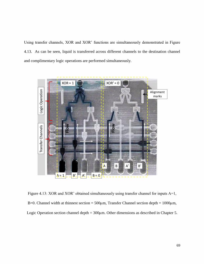
69
Using transfer channels, XOR and XOR‟ functions are simultaneously demonstrated in Figure
4.13. As can be seen, liquid is transferred across different channels to the destination channel
and complimentary logic operations are performed simultaneously.
Figure 4.13: XOR and XOR‟ obtained simultaneously using transfer channel for inputs A=1,
B=0. Channel width at thinnest section = 500m, Transfer Channel section depth = 1000m,
Logic Operation section channel depth = 300m. Other dimensions as described in Chapter 5.
A = 1 B’ A’ B = 0
XOR = 1 XOR’ = 0
Logi
c O
per
atio
nTr
ansf
er C
han
nel
s
Alignment marks
Flo
w
Flo
w
A B’A’B
70
Thus, using the logic scheme described and transfer channels, any logic operation and any
number of operations can be performed.
4.5 Methods
In our study, PMMA (A = 78o, R = 48
o with DI water) was used as the substrate and DI water
was used as the liquid. PMMA pieces were cut and fixed on Microlution‟s micro milling
machine. Inlet and outlet holes were drilled using PMT‟s (www.pmtnow.com) 2mm endmill
(TS-2-0400-S). Thereafter, the pieces were planarized and channels were machined using a 500
micrometer endmill (TS-2-0200-S) using a G-code specifically written for the channel design.
The machining parameters were chosen so as to ensure that the maximum to minimum variation
in depth of the channel was ~2 micrometer. This criterion was chosen arbitrary but it ensured
that the capillary driven fluid flow inside the channel did not pin due to machining marks. The
final machining parameters were RPM = 8000, feed = 50mm/min and step over =0.25 mm. The
devices were bonded using an in house adhesive bonding process developed at the MNMS
cleanroom. Minimal alignment was required during the bonding process as the top plate didn‟t
require machining. During the bonding process, the PMMA pieces were first cleaned with DI
water and ethanol. Adhesive (D75) was applied using a PDMS puck, which was pre-coated with
adhesion promoter (VM752). Thereafter, the devices were bonded in a thermal bonder using the
following process – 1) Press. = 1MPa, Temp = 105 C for 5 min 2) Press. = 1MPa , Cool to 50 C,
1hr.

71
The fabricated XOR and XOR‟ gate with transfer channels (Figure 13) was around 40mm X
40mm in dimension and represented the geometric limit of the microlution machine. More
complicated logic operations can be accomodated using a smaller end mill or via other
fabrication methods like hot embossing [39, 40].
It should be noted that any hydrophilic material can‟t be used as a substrate, especially with
channels of rectangular cross-section, because if the contact angle of the substrate is below 45o,
the edge of the cross section is significantly wetted thereby eliminating the capillary pressure
barrier [41].
4.6 Conclusions
A scalable and cascadable passive microfluidic logic scheme has been designed and a half
adder (AND and XOR gates) was demonstrated using the proposed scheme. Further, using
liquid-walls, a passive „transfer channel‟ scheme is also designed to transport liquid across
the microfluidic chip.
In the logic scheme, no NOT gate is required in such a scheme as complimentary inputs are
provided at the first level of computation and complimentary outputs generated thereafter are
used for cascading. Although this scheme doubles the number of inputs and outputs at each
level but in a practical scenario, one would only generate output and its complimentary only
if they are needed in further logic operations. The first stage of complimentary inputs can be

72
generated in several ways including manual input and hydrogel response [30] based on
physical or chemical stimulus from the environment e.g. pH [31,32], temperature [33, 34],
light [35], pressure [36], biological agents [37] etc. Thus the microfluidic logic scheme could
possibly sense the environmental stimulus and perform logical operations accordingly
thereby acting as a Central Processing Unit (CPU) to perform computations for a passive or
an active device. The output from the logic scheme could be used to further trigger a process
e.g. a hydrogel based valve which controls a chemical reaction. Thus, such a system could
bring cheap computing to diagnostic devices, microfluidic lab-on-chip system, microassays
and related technologies. Also, in environment corrosive to silicon electronics, microfluidic
logic could provide a cheap replacement, although, they can by no means match the speed of
the former.
In its current form, the passive logic device has low robustness to liquid contamination. Thus
the logic scheme would have to be isolated from the external environment possibly using
hydrogels as a communication medium both for input and output. Also, since the device is
passive, it would need to be flushed after one use. This limitation could be overcome by
using a volatile liquid or liquid evaporation by changing device temperature.
4.7 References
1. J. Moorthy, G. A. Mensing, D. Kim, S. Mohanty, D. T. Eddington, W. H. Tepp, E. A.
Johnson, D. J. Beebe, Electrophoresis 25 (2004) 1705.

73
2. C.J. Easley, J. M. Karlinsey, J.M. Bienvenue, L.A. Legendre, M.G. Roper, S.H. Feldman,
M.A. Hughes, E. L. Hewlett, T. J. Merkel, J. P. Ferrance, J. P. Landers, Proc. Natl. Acad.
Sci. 103 (2006) 19272.
3. M.A. Burns, B.N. Johnson, S.N. Brahmasandra, K. Handique, J.R. Webster, M. Krishnan,
T. Sammarco, P.M. Man, D. Jones, D. Heldsinger, C.H. Mastrangelo, D.T. Burke,
Science 282 (1998) 484.
4. R.H. Liu, M.J. Lodes, T. Nguyen, T. Siuda, M. Slota, H.S. Fuji, A. McShea, Anal. Chem.
78 (2006) 4184.
5. K. Sato and T. Kitamori, J. Nanosci. Nanotechnol. 4 (2004) 575.
6. P. Yager, T. Edwards, E. Fu, K. Helton, K. Nelson, M.R. Tam, B.H. Weigl, Nature 442
(2006) 412
7. M. Zimmermann, H. Schmid, P. Hunziker, E. Delamarche, Lab Chip 7 (2007) 119
8. A. Puntambekar, J.W. Choi, C.H. Ahn, S. Kim, V. Makhijani, Lab Chip 2 (2002) 213.
9. K.H. Chung, J.W. Hong, D.S. Lee, H.C. Yoon, Analytica Chimica Acta, 585 (2007) 1.
10. Y. Feng, Z. Zhou, X. Ye, J. Xiong, Sensors and Actuators A, 108 (2003) 138.
11. P.F. Man, C.H. Mastrangelo, M.A. Burns, D.T. Burke, MEMS‟98 pp 45.
12. M.J. Madou, G.J. Kellogg, Proceedings of the SPIE 3259 (1998) 80
13. R.M. Moroney, MSM‟ 98, Santa Clara, CA, 1998 pp. 526
14. Bhushan, Bharat (Ed.), Springer Handbook of Nanotechnology 3rd ed (2010)
15. K. Foster ,G.A. Parker, Fluidics: Components and Circuits, Wiley-Interscience, New
York (1970)
16. T. Vestad, D.W.M. Marr, Applied Physics Letters 84 (2004) 25.
17. M. Prakash, N. Gershenfeld, Science 315 (2007) 832

74
18. A. Groisman, M. Enzelberger, S.R. Quake, Science 300 (2003) 955.
19. W. H. Grover, R. H. C. Ivester, E. C. Jensen, R. A. Mathies, Lab Chip 6 (2006) 623
20. W. Zhan, R. M. Crooks, J. Am. Chem. Soc. 125, no. 33 (2003) 9934
21. J. Melin, N. Roxhed, G. Gimenez, P. Griss, W. Van der Wijngaart, G. Stemme, 12th
International Conference on Transducers, Solid-State Sensors, Actuators and
Microsystems 2 (2003) 1562.
22. Sung-Jin Kim, Yong Taik Lim, Haesik Yang,Yong Beom Shin, Kyuwon Kim, Dae-Sik
Lee, Se Ho Park, Youn Tae Kim., Analytical Chemistry 77, no. 19 (2005) 6494.
23. M. W. Toepke, V. V. Abhyankar, D. J. Beebe, Lab Chip 7 (2007) 1449.
24. T. Young, G. Peacock, editor. Miscellaneous works, London‟ J. Murray, Vol. 1, 1855.
25. Jun Zeng, Manish Deshpande, Ken B. Greiner, John R. Gilbert, ASME 2000.
26. Jerry M. Chen, Po-Chun Huang, Mou-Gee Lin, Microfluid Nanofluid 4 (2008) 427.
27. Jerry M. Chen, Chun-Yi Chen, Chia-Hung Liu, Jap. J. Applied Physics 47, no. 3, (2008)
1683.
28. Hansang Cho, Ho-Young Kimb, Ji Yoon Kang, Tae Song Kim, J. Colloid and Interface
Science 306 (2007) 379.
29. Mano/Kime, Logic and Computer Design Fundamentals, Prentice-Hall Inc.,2nd ed (2001)
30. D. J. Beebe, J.S. Moore, J.M. Bauer, Q. Yu, R.H. Liu, C. Devadoss, B.H. Jo, Nature 404
(2000) 588.
31. D.T. Eddington, D.J. Beebe, Adv. Drug Del. Rev. 56, no. 2 (2004) 199.
32. D.T. Eddington, D.J. Beebe, J. Microelectromech. Syst., 13 (2004) 586.
33. A. Richter, D. Kuckling, S. Howitz, T. Gehring, K-F. Arndt, J. Microelectromech. Syst.,
12 (2003) 748.

75
34. H. J. Van der Linden, W. Othuis, P. Bergveld, Lab Chip, 4 (2004) 619.
35. A. Suzuki, T. Tanaka, Nature, 346 (1990) 345.
36. K.K. Lee, E.L. Cussler, M. Marchetti, M.A. McHugh, Chem. Eng. Sc. 45 (1990) 766.
37. T. Miyata, N. Asami , T.A. Uragami, Nature 399 (1999) 766.
38. T. Malik, N.X. Fang, “Flow Inside Microchannels With Liquid-Walls”, ASME Conf.
Proc. 921 (2008), DOI:10.1115/IMECE2008-67546
39. T. Koerner,L. Brown, R. Xie, R.D. Oleschuk, Sensors and Actuators B 107 (2005) 632.
40. L.J.Kricka,P. Fortina, N.J. Panaro, P. Wilding, G. Alonso-Amigoc, H. Becker, Lab on a
Chip 2 (2002) 1.
41. E. Kim, G.M.J. Whitesides, Phys. Chem. B. 101 (1997) 855.

76
5. WALL-LESS FLOW IN MICROCHANNELS
Microfluidic flows are characterized by high surface-area to volume ratio resulting in dominant
interfacial-forces. Many researchers have used this to their advantage and designed microfluidic
pumping systems [1], self-fluid replacement mechanisms [2] etc. Further, surface and geometry
modulation have extended the capability to exploit these effects to design microfluidic valves
[3,4,5,6].
Recently, selective surface patterning has been used to confine microfluidic flow using only two
physical walls [7]. Although, such a system offers the ability to define hydrophobic/hydrophilic
pathways with varying shapes, dynamic manipulation of pathways is not possible. Also, the
advancing contact angle of the liquid on the hydrophobic region limits the maximum pressure
that the „liquid-walls‟ can sustain and the hydrophobic/hydrophilic pathways can be washed
away over time. This constraints the use of these systems at microscale.
(a) (b)
Figure 5.1: Liquid-wall using selective chemical patterning a) Liquid in microfluidic channel
with only two physical walls b) Chemical patterning used for a) [7]
Hydrophilic
Hydrophobic

77
In this study, liquid-wall is created on hydrophilic substrate by using geometric modulation and
without the need for hydrophobic patterning. A theoretical model has been developed to
calculate the channel geometry required to create a liquid-wall. Thereby, a microfluidic channel
is fabricated and liquid-wall flow is demonstrated. This scheme is used in designing „transfer-
channels‟ to passively control the transfer of liquid in a multi-layered microfluidic device. The
„transfer-channels‟ are thereby used to add scalability to passive liquid-logic, demonstrated in
previous chapter. The scheme can be also be used in liquid-gas chemical reactors, passive
microfluidic valves, microfluidic pressure switches and in eliminating air entrapment issues.
5.1 Theory
A sudden expansion in flow cross-section can stop a liquid stream driven by capillary force and
this principle has been used to design passive microfluidic AND gate [3,5,6,8,9]. Using the same
basic principle, I demonstrate the creation of liquid-wall using a channel design shown in Figure
5.2.
As can be seen, two hydrophilic substrates are bonded together to form the microfluidic
channels. The bottom plate has two channels, where the depth of one is more than the other. As
the liquid is introduced in the shallower channel, it is driven by capillary force. This flowing
liquid then encounters a sudden difference in the depth perpendicular to the flow direction. If
properly dimensioned, the liquid forms a meniscus which stops it from spilling into the deeper
channel thereby creating a liquid-wall. The liquid-wall can also sustain a pressure driven flow
until the pressure is below a critical value.

78
Figure 5.2: a) Schematic of channel geometry for liquid-wall flow (L – length of liquid wall, W-
height of liquid-wall, – expansion angle, T – width of inflow channel)
For a static liquid-wall, the pressure required to break the same can be calculated by using
Young‟s equation [10] –
<5.1>
Where, Max.[(a)], Max.[(a)], Max.[(a)] = 180o, a is the advancing contact angle
of the liquid on solid substrate, is the surface tension of the liquid, and g are liquid density
and acceleration due to gravity respectively. It can be seen that the depth of the deeper channel
isn‟t one of the design parameters and can be chosen arbitrarily. The second term on the left hand
side of the equation accounts for the maximum pressure on the liquid-wall due to the weight of
the liquid. This contribution can be neglected for sub-millimeter deep channels.
Neglecting liquid weight and non-dimensionalizing equation 5.1 –
Liquid-wall
Liquid-wall
LWaLaL
aWWgbreak
P
*/)]3cos(*)2cos(*
)1cos(*2[**

79
<5.2>
Figure 5.3 shows the plot of break pressure for different depths of the shallower channel and
different lengths of the liquid-wall. The liquid assumed is water and the substrate assumed is
Polymethylmethacrylate or PMMA (a = 78o with DI water). The parameters used for the graph
were 1 = 90o, 2 = 90
o, 3 = 0
o, 4 = 90
o and width, T = 500m.
Figure 5.3: Break pressure for different dimensions of the liquid wall with varying aspect ratio
(1 = 90o, 2 = 90
o, 3 = 0
o, 4 = 90
o and width, T = 500m). Refer Figure 5.2
It should be noted that equations 5.2 has been quantitatively validated by various researchers
[11 - 14] for several different substrate and liquid combinations. Further, since the scope of
the work is limited to qualitaive validation of liquid-wall, only the same is demonstrated
0
500
1000
1500
2000
2500
3000
0 10 20 30 40 50
No
n d
imen
sio
nal B
reak P
ressu
re
Aspect ratio of liquid wall (w/L)
w = 20 microns
w = 100 microns
w = 500 microns
)3cos()2cos()1cos(*)/(2*
aaaLWW
breakP

80
here.
In case of a pressure driven flow, the break pressure of the liquid-wall determines the maximum
length of the flow channel, for a given flow rate . This is because the pressure drop is a function
of flow rate and flow resistance. For a constant flow rate, the flow resistance keeps increasing as
the liquid fills the microfluidic channel and thus the inlet pressure must be increased accordingly.
Thus, since the break pressure is constant, as the flow length increases, the liquid-wall breaks.
For a capillary driven flow, since inlet pressure is constant, the flow rate automatically adjusts to
balance the pressure gradient and thus the flow length is not restricted in such a scenario.
Also, it can be seen from Figure 5.2 that as the liquid flows in and forms liquid-wall, it
encounters a sudden expansion (angle 4). Thus, it should be ensured that the liquid doesn‟t stop
at this expansion. This can be ensured by sizing the inflow channel width, T so that the break
pressure to overcome the particular sudden-expansion is negative –
5.2 Methods
In our study, Polymethylmethacrylate or PMMA (A = 78o, R = 48
o with DI water) was used as
the substrate and DI water was used as the liquid. 2X4 cm PMMA pieces were cut and fixed on
Microlution‟s micro milling machine. Inlet and outlet holes were drilled using PMT‟s
(www.pmtnow.com) 2mm endmill (TS-2-0400-S). Thereafter, the pieces were planarized and
TWTWW
PwhereP
aaa
breakbreak
*/]cos*2cos*)cos(*[*
)(, 0
4

81
channels were machined using a 500 micrometer endmill (TS-2-0200-S) using a G-code
specifically written for the channel design.
The machining parameters were chosen so as to ensure that the maximum to minimum variation
in depth of the channel was ~2 micrometer. This criterion was chosen arbitrary but it ensured
that the capillary driven fluid flow inside the channel did not pin due to machining marks. The
final machining parameters were RPM = 8000, feed = 50mm/min and step over =0.25 mm. The
devices were bonded using an in house adhesive bonding process developed at the MNMS
cleanroom. No alignment was required during the bonding process as the top plate didn‟t require
machining. During the bonding process, the PMMA pieces were first cleaned with DI water and
ethanol. Adhesive (D75) was applied using a PDMS puck, which was pre-coated with adhesion
promoter (VM752). Thereafter, the devices were bonded in a thermal bonder using the following
process – 1) Press. = 1MPa, Temp = 105 C for 5 min 2) Press. = 1MPa , Cool to 50 C, 1hr.
It should be noted that any hydrophilic material can‟t be used as a substrate, especially with
channels of rectangular cross-section, because if the contact angle of the substrate is below 45o,
the edge of the cross section is significantly wetted thereby eliminating the capillary pressure
barrier [15].
5.3 Liquid-wall demonstration
In the study, I used PMMA as our substrate and DI water was used as the liquid. The parameters
used for fabrication were 1 = 90o, 2 = 90
o, 3 = 0
o, 4 = 90
o and width, T = 500m. The
channel length was arbitrarily chosen to be 13 mm and the device depth was calculated to be 200

82
m. Figure 5.4 shows the water-wall formed after the water fills the channel. When water is
introduced into the adjacent empty channel, it instantly „switches-off‟ the water wall by filling
the empty channel.
Figure 5.4: Water in the channel confined by water- wall
5.4 ‘Transfer-channel’ design
Liquid-wall is used to design „transfer-channels‟ to passively control the transfer of liquid in a
multi-layered microfluidic device. This is shown in Figure 5.5, 5.6 and 5.7.
In the figure 5.5, two criss-crossing channels, 1 and 2, are shown with channel 1 containing
liquid. It can be seen that channel 1 is in bottom part or substrate and channel 2 is in the top part
or cover of the device, forming a two-layered microfluidic channel network. As the liquid flows
in channel 1, it forms a liquid-wall at the junction where the channels criss-cross. By controlling
the dimensions of the liquid-wall at the junction, the flow of liquid from channel 1 to channel 2
can be controlled.
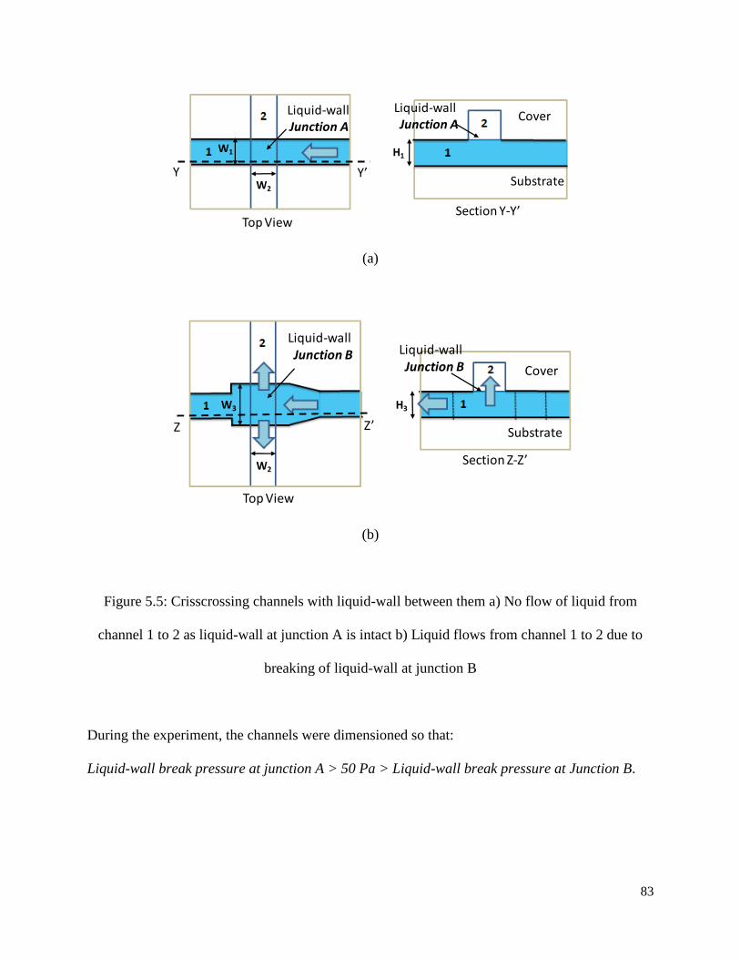
83
(a)
(b)
Figure 5.5: Crisscrossing channels with liquid-wall between them a) No flow of liquid from
channel 1 to 2 as liquid-wall at junction A is intact b) Liquid flows from channel 1 to 2 due to
breaking of liquid-wall at junction B
During the experiment, the channels were dimensioned so that:
Liquid-wall break pressure at junction A > 50 Pa > Liquid-wall break pressure at Junction B.
W1
W2
Cover
Substrate
Liquid-wallJunction A
Liquid-wallJunction A
H1
Y Y’
Section Y-Y’Top View
Substrate
Cover
W3
W2
H3
Z Z’
Section Z-Z’
Top View
Liquid-wallJunction B
Liquid-wallJunction B

84
Here, 50 Pa represents the positive pressure due to the curvature of the liquid drop placed at the
inlet. This positive pressure at inlet is used to break the liquid-wall at junction B without
breaking the liquid wall at junction A, thereby allowing controlled transfer of liquid. Further, the
depth of the channels 1 and 2 are so dimensioned so as to allow the formation of liquid wall at
junction A and junction B. The calculations are done using equation 5.1.
The channels have been dimensioned for a combination of DI water (LA = 0.072 N/m @ 25oC)
and PMMA (a for DI water = 78o @ 25
oC, 50% RH). The resultant dimensions are: W1 = W2 =
500 m, W3 = 1600 m and H1 = H3 = 1000 m. The break pressure of liquid wall at junctions
A and B are shown in Table 5.1.
Junction Break Pressure (Pa)
Liquid-wall Junction A 219.5
Liquid-wall Junction B 24.1
Table 5.1: Break pressure for different liquid-wall junctions
Using the criss-crossing channel scheme in Figure 5.5, a two layered microfluidic device is
designed to passively control the transfer of liquid from a given inlet channel to a given outlet
channel. This is shown in Figure 5.6.

85
(a) Bottom layer of microfluidic channels
(b) Top layer of channels
(c) Assembled device
(d) Cross-sectional view across A-A, showing transfer of liquid
Figure 5.6: Schematic of passive transfer of liquid across microfluidic channels
25o
500m
1600m
1800mchannel depth = 1000m
Through holes
500m
25o
1600m
1800m
Through holes
channel depth = 1000m
1 2
Inlet Outlet
A A
Top layer
Bottom layer1
2
Liquid-wall intact
Liquid-wall breaks
Liquid-wall breaks
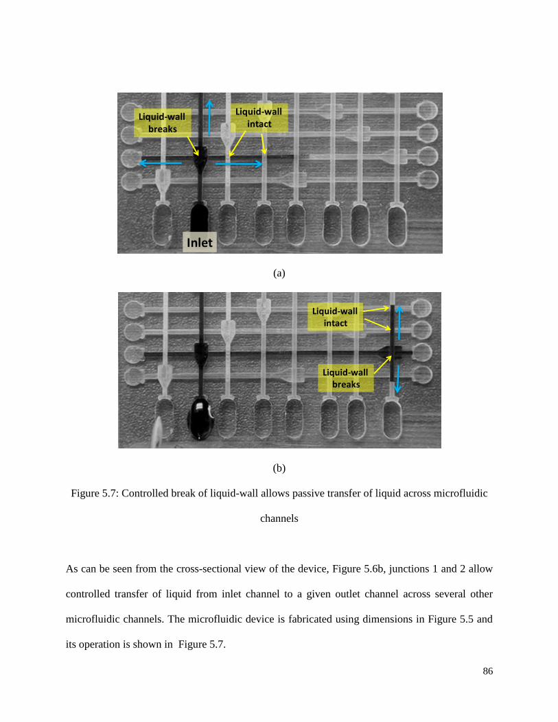
86
(a)
(b)
Figure 5.7: Controlled break of liquid-wall allows passive transfer of liquid across microfluidic
channels
As can be seen from the cross-sectional view of the device, Figure 5.6b, junctions 1 and 2 allow
controlled transfer of liquid from inlet channel to a given outlet channel across several other
microfluidic channels. The microfluidic device is fabricated using dimensions in Figure 5.5 and
its operation is shown in Figure 5.7.
Inlet
Liquid-wall breaks
Liquid-wall intact
Liquid-wall breaks
Liquid-wall intact

87
However, the demonstrated „transfer channel‟ scheme requires that a slight positive pressure is
always maintained at the inlet to break the liquid-wall and transfer the liquid. But as the liquid
fills the channels, the pressure at the inlet drop will go down. This problem can be solved by
connecting all the channels to a liquid reservoir, with a fresh drop volume, at regular intervals.
This is shown in Figure 5.8. As can be seen, the liquid from the new drop forms a liquid wall
with each channel. When the channels carrying liquid come in contact with the liquid reservoir,
through the liquid-wall, the pressure in the system increases for the next set of operations (due to
the pressure being higher in the reservoir channel). Further, the reservoir liquid-wall is designed
so as to keep it intact, as shown earlier.
(a)
(b)
Figure 5.8: Reservoir channel is used to increase the inlet pressure downstream (a) Top view of
reservoir channel forming liquid-wall with input channels (b) Section X-Y
X Y
ReservoirReservoir channel
Liquid wall
Input channels
Liquid wall
Reservoir channel
Reservoir Input channels

88
5.5 Summary
Liquid-wall flow has been accomplished in a microfluidic device, without the use of surface
patterning. The walls in the designed channel can be manipulated dynamically by simply
introducing liquid into the adjacent channel, thus turning them „off‟. A theoretical model has
been developed for predicting the break pressure of the liquid-wall. Further, geometrically
manipulated breaking of liquid-wall has been used to control the transfer liquid into desired
microfluidic channels in a multi-layered microfluidic device.
Also, given the significant liquid-gas interface area offered by liquid-walls, they could form
artificial-lungs for chemical analysis [7]. Fabrication of such channels with intermittent side
walls could make these systems practical by keeping the break pressure of the liquid-wall high
with little compromise on the liquid-gas interface area. Pressure driven flow in such a system
would be limited by the length of flow channel for a given flow rate.
Additional Information Available
Appendix B shows the calculations for the limit in height of the liquid-wall.
5.6 References
1. Zimmermann, M., Schmid, H., Hunziker, P., Delamarche, E., Lab on a Chip, 7, 119-125 ,
2007.

89
2. Chung, K.H., Hong, J. W., Lee, D.S., Yoon, H.C., Analytica Chimica Acta, 585, 1-10,
2007
3. Feng, Y., Zhou, Z., Ye, X., Xiong, J., Sensors and Actuators A, 108, 138 – 143, 2003
4. Zhao, B., Moore, J. S., Beebe, D. J., Langmuir, 19, 1873-1879, 2003
5. Man, P. F., Mastrangelo C. H., Burns M. A. and Burke D. T., MEMS‟98, pp 45–50, 1998
6. Madou, M.J., Kellogg, G.J., Proceedings of the SPIE, Vol. 3259, pp. 80–93, 1998
7. Zhao, B., Moore, J. S., Beebe, D. J., Science, 291, 1023-1026, 2001
8. R.M. Moroney, MSM‟ 98, Santa Clara, CA, 1998 pp. 526 ; J. Melin, N. Roxhed, G.
Gimenez, P. Griss, W. Van der Wijngaart, G. Stemme, 12th International Conference on
Transducers, Solid-State Sensors, Actuators and Microsystems 2 (2003) 1562.
9. Sung-Jin Kim, Yong Taik Lim, Haesik Yang,Yong Beom Shin, Kyuwon Kim, Dae-Sik
Lee, Se Ho Park, Youn Tae Kim., Analytical Chemistry 77, no. 19 (2005) 6494
10. T. Young, G. Peacock, editor. Miscellaneous works, London‟ J. Murray, Vol. 1, 1855
11. Jun Zeng, Manish Deshpande, Ken B. Greiner, John R. Gilbert, ASME 2000.
12. Jerry M. Chen, Po-Chun Huang, Mou-Gee Lin, Microfluid Nanofluid 4 (2008) 427.
13. Jerry M. Chen, Chun-Yi Chen, Chia-Hung Liu, Jap. J. Applied Physics 47, no. 3, (2008)
1683.
14. Hansang Cho, Ho-Young Kimb, Ji Yoon Kang, Tae Song Kim, J. Colloid and Interface
Science 306 (2007) 379.
15. E. Kim, G.M.J. Whitesides, Phys. Chem. B. 101 (1997) 855

90
APPENDIX A: Determination of trapped volume and modified Gibbs Energy Barriers
The geometry of the roughness profile physically limits the states accessible to the drop. This has
been discussed in detail in the paper and here I present the calculations used to determine the
trapped volume and the modified Gibbs energy barriers.
Consider Figure A.1, the two triangles show the roughness features and B1‟-B1 and B2‟-B2-C2
represent the tangents at the liquid-air interface, at the point of contact of liquid with the solid,
for metastable state B1 and an intermediate state C2 respectively. A co-ordinate system is
established with C1 as the origin. Further, as mentioned in the paper, it is assumed that the drop
has a single radius of curvature at any given x.
It has been pointed out that C2 is a non-equilibrium state and therefore the results from the
calculations should be interpreted only qualitatively.
A.1: Calculation of trapped volume
As the volume of the drop is constant,
Volume of drop at B1 = Volume of drop at C2 < A.1.1>
Where, Volume of drop at B1 = f (x, b, Pitch) and Volume of drop at C2 = f (x, b, Pitch),
and can be calculated as described in the paper.

91
Figure A.1: Schematic of liquid-air interface for a 2D drop
Since B2 (-P/2, P/2*tanb) and C2 (xs, xs*tan ) lie on line B2‟-C2, equation for the line B2‟-C2
is:
<A.1.2>
The values of xs and can be found by solving simultaneous equations A.1.1 and A.1.2.
The trapped volume, Vsm given by the area of triangle B2-C1-C2 is calculated as:
<A.1.3>
P/2
C1
B1B2
C2
xs
B1’
B2’
1
b
x
bb tan*2/tan*)2/(tan PPxx ss
btan*2/**2 PxVsm s

92
A.2: Calculation of Gibbs energy for trapped volume
To calculate Gibbs energy of the trapped volume, it is assumed that when the drop moves to
metastable state B2, the trapped volume attains minimum energy state by intersecting the sides
of the roughness features at Young‟s contact angle. This is shown in Figure A.2. The curvature
of the liquid-air interface for the trapped volume is neglected and the energy is given as:
<A.2.1>
Where,
As stated earlier, LA has been assumed to be 1 for this study.
Figure A.2: Trapped volume
Trapped volume
W
btan/*2 VsmW
)2]cos
2[*cos(.Re W
WlGE YLATrappedVol
b

93
A.3: Calculation of modification in Gibbs energy barriers
The modified Gibbs energy barrier for metastable state B1 is given as:
GEB-L(B1) MOD = GEC2 – GEB1
The relative Gibbs energy (GE) of the drop at point C2 and B1 can be determined by using
equation 6, as xs, and are known.
GEB-S for state B2 is similarly affected and can be calculated as:
GEB-S (B2) MOD = GEB2 – GEC2.
To determine the relative GE at point B2, Vsm is subtracted from the drop volume and thereafter
equation 6 is used along with volumetric constraint for calculations. The energy of the trapped
volume is also included in the total energy of the system.

94
APPENDIX B: Maximum height and radius of curvature for liquid-wall flow
The maximum depth of the flow channel is determined by the weight of liquid that the liquid-
meniscus can sustain. The same can be calculated by using Young‟s equation –
<B.1>
Where R1 and R2 are the radii of curvature of the liquid-wall. Assuming R2>> R1, implying
length of liquid-wall is much greater than its height -
<B.2>
Noting from geometry that 1/R1 = d/dS, where S is the length of the meniscus and non-
dimensionalizing the equation using capillary length - lo = sqrt(/g),
<B.3>
In the above equation, the lower case subscripts - s, r2, w and y represent non-dimensionalized S,
R2, W and Y respectively. Equation B.3 has been solved by Saif et al. [Saif, T., J. Fluid Mech.,
473 (2002) 321]. Using the same method, it can be shown that –
<B.4>
WLYWgR
P );()1
1(
)( ywds
d
)sin(cos2
0
2
w
)2
1
1
1(
RRP

95
Or,
<B.5>
For water, the maximum height turns out to be ~3.8mm for a contact angle of 90o (considering
only hydrophilic substrates)
Figure B.1: Schematic of liquid meniscus forming the liquid-wall
Similarly, the maximum radius of curvature that the liquid-flow can make is restricted by the
break pressure of the liquid-wall. As the liquid-flow turns, the radius of curvature on the inside
of the turn is of opposite sign to the one made by liquid meniscus/liquid-wall. Thus, the liquid-
wall can break in such a situation. The max. radius of curvature can be calculated by equating the
break pressure to zero –
w
Rc
Rc << W
d
dS
dx
dy
(0,0)
R1
c
)cos(sin2 0
gW

96
<B.6>
Figure B.2: Co-ordinate system set-up for radius of curvature calculation
Neglecting the contribution due to the weight of liquid, R2, max = |R1|. R1 can be calculated by
solving the following simultaneous equations (Figure B.2) –
<B.7>
<B.8>
<B.9>
<B.10>
a
(0,W)
R1
c
a
(c1,0)
R1
c
(0,0)
(x1,y1)
22
22
)11(1
)1(11
)90tan(*)11(1
tan*11
ycxR
WyxR
cxy
Wxy
a
a
WgRR
Pbreak *)2
1
1
1(0

97
Table B.1: Max. radius of curvature for liquid-wall flow
Height of liquid-wall
(microns)
Max. radius of curvature
(microns)
100 141
200 283
500 707
98
Author’s Biography
Tarun Malik was born on March 25th, 1981 in New Delhi, India. He received his B.E. degree in
Mechanical Engineering from Delhi College of Engineering, Delhi, India in 2002. Tarun then
joined Department of Mechanical Engineering at University of Illinois, Urbana-Champaign in
August 2004 to pursue M.S. He worked with Prof. Clark Bullard on his Master‟s thesis:
„Exploring component design and system tradeoff‟ and was part of the Air Conditioning and
Refrigeration Center (ACRC). Thereafter, he joined Behr America, an automotive air-
conditioning company based in Troy, MI in August, 2004. After two years of experience, he
decided to pursue PhD and returned to University of Illinois in August 2006. He joined Prof.
Nicholas X. Fang‟s group in January 2007. His research has been focused on understanding
solid-liquid interfacial phenomena and developing applications based on the same. After
receiving his Ph.D., Tarun will join Intel Corporation in Portland, Oregon.