study of conformational changes in conjugated organic … · high-pressure apparatus ... high...
TRANSCRIPT

INFRARED SPECTROSCOPY OF CONJUGATED
ORGANIC MOLECULES UNDER HIGH PRESSURE
By
KIRILL KHAMIDOVICH ZHURAVLEV
A dissertation submitted in partial fulfillment of the requirements for the degree of
Doctor of Philosophy
WASHINGTON STATE UNIVERSITY Department of Physics
MAY 2004
©Copyright by KIRILL KHAMIDOVICH ZHURAVLEV, 2004 All Rights Reserved

©Copyright by KIRILL KHAMIDOVICH ZHURAVLEV, 2004 All Rights Reserved

To the Faculty of Washington State University:
The members of the Committee appointed to examine the dissertation of Kirill
Khamidovich Zhuravlev find it satisfactory and recommend that it be accepted.
___________________________
Chair
___________________________
___________________________
ii

Acknowledgements
I would like to thank my advisor, Dr. Matthew D. McCluskey, for suggesting
this project and for his constant support and assistance through the course of this
work. His help and guidance can not be overestimated. I would also like to thank Dr.
Zbignew Dreger for his help with fluorescence system and Dr. Eugene Haller for
providing us with germanium detectors. Brooke Bafus work on taking p-quaterphenyl
spectra was very supportive and Slade Jokela’s help with the vapor deposition system
is extremely highly appreciated.
I personally want to thank my beloved wife Valentina for her understanding
and constant help and love, which created a supportive and warm atmosphere in our
home, and also for bringing our two sons, Michael and Nicholas, into the world.
iii

INFRARED SPECTROSCOPY OF CONJUGATED
ORGANIC MOLECULES UNDER HIGH PRESSURE
Abstract
By Kirill Khamidovich Zhuravlev, Ph.D.
Washington State University
May 2004
Chair: M. D. McCluskey
Conjugated organic molecules are important components in solid-state
optoelectronic devices and laser dyes. Changes in the conformations of these
molecules affect the optical emission wavelengths. In order to probe the conformation
of conjugated molecules, infrared (IR) spectroscopy was performed on organic solids
under high hydrostatic pressures.
We investigated polyphenyl molecules, such as biphenyl, p-terphenyl, and p-
quaterphenyl. It was shown that polyphenyl molecules experience a phase transition
in which molecules change their conformation from a twisted to a planar structure.
This transition manifests itself in dramatic changes in the IR spectra. Beyond a
critical pressure, specific IR-active modes abruptly become IR-inactive.
IR spectra have been obtained with a Bomem DA8 Fourier-Transform IR
spectrometer in the 500-5000 cm-1 spectral range. Those spectra clearly showed that
when the pressure increases above the critical value some IR-peaks completely
iv

disappear from the spectrum. The critical pressure was found to range from 0.2 GPa
for biphenyl to 0.9 GPa for p-quaterphenyl molecule.
Numerical analysis of conjugated molecules has been done using ab initio
calculations. Using the local density approximation, calculations of molecular
structure, vibrational frequencies, and IR intensities were performed. The results of
these numerical simulations confirmed the experimental observations and allowed us
to resolve a controversy about the p-terphenyl structure in the twisted conformation.
They also demonstrated that high-pressure IR spectroscopy can be a very sensitive
tool in probing molecular structure.
In order to investigate the effect of pressure, as dimensions approach the
nano-scale, IR spectroscopy was performed on nm-thick organic films. The special
technique called surface-enhanced infrared absorption spectroscopy (SEIRA) has
been applied to the investigation of a thin film (30 nm) of p-nitrothiophenol under
high pressure. The phenomenon of absorption enhancement in the presence of thin
metal film has been used to obtain the absorption spectra of thin layer of p-
nitrothiophenol.
v
Table of contents
Acknowledgements............................................................................................................ iii
Abstract .............................................................................................................................. iv
List of Tables: ......................................................................................................................x
List of figures:.................................................................................................................... xi
1. Objectives of this work ....................................................................................................1
2. Organization of thesis ......................................................................................................2
3. Theoretical background ...................................................................................................3
3.1 Methods of quantum chemistry. ................................................................................ 3
3.1.1. Self-consistent field theory. .............................................................................. 3
3.1.2. Thomas-Fermi theory........................................................................................ 6
3.1.3. Density-functional theory. ................................................................................ 7
3.1.4. Molecular structure determination.................................................................. 10
3.1.5. Group theory. .................................................................................................. 11
3.1.6. Examples of point groups. .............................................................................. 13
3.1.7. Mathematical background............................................................................... 16
3.1.8. Application of group theory to molecular vibrations...................................... 17
3.2. Numerical calculations............................................................................................ 23
3.3. Theory of phase transitions..................................................................................... 25
3.3.1 General properties of phase transitions............................................................ 25
3.3.2. First-order phase transitions............................................................................ 27
3.3.3. Second-order phase transitions. ...................................................................... 27
3.2.5. Correlation function. ....................................................................................... 32
vi

3.2.6. Scaling hypothesis. ......................................................................................... 33
3.4. Incommensurate phases in dielectrics..................................................................... 35
3.4.1. Phenomenological theory of incommensurate phases. ................................... 35
3.4.2. Microscopic theory of incommensurate phase. .............................................. 40
4. Conjugated molecules....................................................................................................43
4.1. Organic laser dyes and light-emitting devices (OLED).......................................... 43
4.1.1. Organic dyes. .................................................................................................. 43
4.1.2. Organic light-emitting devices (OLEDs)........................................................ 44
4.2. Conjugated molecules and their investigation. ....................................................... 50
4.2.1. Introduction..................................................................................................... 50
4.2.2. Biphenyl.......................................................................................................... 52
4.2.3. P-terphenyl...................................................................................................... 56
4.2.4. P-quaterphenyl. ............................................................................................... 58
5. Experimental methods. ..................................................................................................59
5.1. High-pressure apparatus.......................................................................................... 59
5.1.1. Diamond-anvil cells. ....................................................................................... 59
5.1.2. Diamond-anvil cell alignment......................................................................... 66
5.1.3. Diamond-anvil cell loading............................................................................. 67
5.1.4. Low-temperature measurements..................................................................... 67
5.1.5. Fluorescence measurement system. ................................................................ 68
5.2. Fourier transform infrared spectroscopy (FT-IR). .................................................. 69
5.2.1. Basic theory of FT-IR. .................................................................................... 69
5.2.2. Beer’s Law. ..................................................................................................... 73
vii

5.2.3. Beamsplitters for FT-IR spectrometers........................................................... 74
5.2.4. Infrared detectors. ........................................................................................... 75
5.3. Advantages of FT-IR spectrometers. ...................................................................... 76
5.3.1. Jacquinot’s advantage. .................................................................................... 76
5.3.2. Fellgett’s advantage. ....................................................................................... 77
5.3.3. Fourier-transform infrared (FT-IR) spectrometry........................................... 77
6. Present work...................................................................................................................79
6.1. Organic conjugated molecules under pressure. ...................................................... 79
6.1.1. Biphenyl.......................................................................................................... 79
6.1.1.1. Experimental results..................................................................................79
6.1.1.2. Group theory. ............................................................................................84
6.1.1.3. Numerical calculations..............................................................................86
6.1.1.4. Conclusions...............................................................................................91
6.1.2. P-terphenyl...................................................................................................... 93
6.1.2.1. Experimental results..................................................................................93
6.1.2.2. Numerical calculations..............................................................................98
6.1.2.3. Group theory. ............................................................................................99
6.1.2.4. Comparison between theory and experiment..........................................100
6.1.2.5. Conclusions.............................................................................................103
6.1.3. P-quaterphenyl. ............................................................................................. 104
6.1.3.1. Experimental results................................................................................104
6.1.3.2. Group theory. ..........................................................................................105
6.1.3.3. Conclusions.............................................................................................108
viii

6.2. Surface-enhanced Infrared (SEIRS) and............................................................... 110
Raman (SERS) Spectroscopy. ..................................................................................... 110
6.2.1. General description of the method................................................................ 110
6.2.2. Electromagnetic (EM) mechanism of surface-enhanced absorption. ........... 112
6.3. Thin films of organic molecules under pressure.......................................................116
6.4. Current research. ................................................................................................... 118
6.4.1. Film preparation............................................................................................ 118
6.4.2. Results........................................................................................................... 121
7. Summary of results ......................................................................................................123
8. Future work directions .................................................................................................124
9. List of publications ......................................................................................................125
APPENDIX A..................................................................................................................126
Absorption of light. Quantum-mechanical treatment. ................................................. 126
APPENDIX B. .................................................................................................................128
Isotopic shift of the vibrational frequency of the molecule. ........................................ 128
APPENDIX C. .................................................................................................................130
Frequency distribution for the system of oscillators.................................................... 130
with nearest-neighbor interaction. ............................................................................... 130
Appendix D......................................................................................................................134
AFM images of thin film of p-NTP. ............................................................................ 134
References:.......................................................................................................................136
ix

List of Tables:
I. GAUSSIAN98 basis sets and their characteristics.
II. Pressure media and their characteristics.
III. Vibrational modes in biphenyl that lose IR activity upon planarization.
IV. Vibrational modes in deuterated biphenyl that lose IR activity upon
planarization.
V. Ground-state energies of various conformations of p-terphenyl relative to
planar conformation.
x
List of figures:
1. Water molecule.
2. Hydrogen peroxide molecule.
3. Benzene molecule.
4. Vibrational eigenmodes of the water molecule.
5. Schematic representation of the energy levels and electronic transitions of an
organic molecule used in laser dyes.
6. Design of the light-emitting device (LED).
7. Schematic phase diagram of biphenyl.
8. Effective molecular potential at low and high pressures.
9. Schematic picture of the National Bureau of Standards (NBS) diamond-anvil
cell (DAC) design.
10. Schematic picture of the Bassett diamond-anvil cell (DAC) design.
11. Schematic picture of the Mao-Bell diamond-anvil cell (DAC) design.
12. Schematic picture of the Syassen-Holzapfer diamond-anvil cell (DAC) design.
13. Schematic picture of the Merill-Bassett diamond-anvil cell (DAC) design.
14. Schematic representation of the low-temperature high-pressure IR-
spectroscopy device.
15. Michelson interferometer.
16. Biphenyl spectra at pressures below and above phase transition. IR-modes,
that disappear upon transition, are indicated by arrows.
xi

17. Deuterated biphenyl spectra at pressures below and above phase transition.
IR-modes, that disappear upon transition, are indicated by arrows.
18. Frequency dependence of several IR-modes on the pressure for biphenyl.
19. Normalized intensity dependence on the pressure for two IR-modes that
become IR-inactive upon phase transition for the biphenyl molecule.
20. Biphenyl molecule structure in the twisted conformation.
21. Schematic representation of the mechanism of IR-activity loss for one of the
hydrogen out-of-plane modes for the biphenyl molecule.
22. Calculated intensity dependence of two IR-modes on the twist angle between
two phenyl rings in the biphenyl molecule.
23. Comparison between experimental and calculated frequencies for biphenyl
and deuterated biphenyl modes that become IR-inactive upon phase transition.
24. Three possible isomers of p-terphenyl molecule in the twisted conformation.
25. P-terphenyl spectra at pressures below and above phase transition. IR-modes,
that disappear upon transition, are indicated by arrows.
26. Deuterated p-terphenyl spectra at pressures below and above phase transition.
IR-modes, that disappear upon transition, are indicated by arrows.
27. Frequency dependence of several IR-modes on the pressure for p-terphenyl.
28. Comparison between experimental and calculated frequencies for p-terphenyl
modes that become IR-inactive upon phase transition for different possible
twisted conformations.
xii

29. Comparison between experimental and calculated frequencies for deuterated
p-terphenyl modes that become IR-inactive upon phase transition for different
possible twisted conformations.
30. P-quaterphenyl molecule structure in the planar and twisted conformation.
31. P-quaterphenyl spectra at pressures below and above phase transition. IR-
modes that disappear upon transition are indicated by arrows.
32. Frequency dependence of several IR-modes on the pressure for p-
quaterphenyl and normalized area dependence on the pressure for an IR-mode
that become IR-inactive upon phase transition for p-quaterphenyl molecule.
33. Critical pressure as a function of the number of phenyl rings.
34. Comparison between experimental and calculated frequencies for p-
quaterphenyl modes that become IR-inactive upon phase transition.
35. The schematic picture of the vapor deposition system used in depositing thin
silver films onto diamond.
36. Typical IR spectra of p-NTP film at different pressures.
37. Pressure dependence of NO2 symmetrical stretch mode frequency in p-NTP
film.
38. AFM image of the thin film of p-NTP on silver.
39. Same as in Fig. 38, but with cross-sectional profile showing height
distribution.
xiii

1. Objectives of this work
The application of high pressure is widely used in physical experiments to study
the properties of condensed-matter systems. It is known that pressure can change solid-
state structures and induce various phase transitions in materials. Novel structures can be
synthesized using high pressure, which are important for both technological applications
and fundamental research.
The objective of this work was to investigate the behavior of organic solids under
high hydrostatic pressure. Among all organic solids we chose conjugated molecules,
which have wide applications in organic light-emitting devices and laser dyes. Those
molecules are known to undergo phase transitions when either temperature or pressure
rises above critical values.
Specific objectives included studying the optical properties of polyphenyl
(biphenyl, p-terphenyl, and p-quaterphenyl) solids, numerical simulations of molecular
structures, and investigation of thin films of p-nitrothiophenol (p-NTP), when the solid
becomes quasi-two-dimensional. We obtained infrared (IR) spectra of those solids and
thin films using Fourier-transform infrared spectrometry and we used diamond-anvil cells
to generate high pressures up to 10 GPa. By obtaining the vibrational spectra as a
function of pressure, phase transitions were observed.
An essential part of this work was the comparison between the calculations and
the experimental data. Toward that end, we performed ab initio calculations of molecular
structure and vibrational properties of the molecules under investigation and compared
those results with experiment. In the case of biphenyl, for which the structure is well
1

known, the comparison between theory and experiment provided a validation of our
approach. For p-terphenyl, the combined theoretical and experimental techniques yielded
information about its molecular structure.
2. Organization of thesis
Section 3 reviews the theory behind phase transitions and models for quantum
chemistry. Hartree-Fock, Thomas-Fermi, and density-functional theory are considered for
modeling molecular structures. The basics of numerical calculations are presented.
Landau theory and scaling hypotheses, along with the notion of imcommensurate phases,
are described.
Section 4 reviews applications and methods of investigation of organic solids,
along with some results on polyphenyl molecules.
Section 5 describes the high-pressure apparatus and Fourier-Transform IR (FT-
IR) spectroscopy technique. Some attention is given to in situ pressure measurements,
infrared detectors, and comparative advantages of FT-IR with respect to grating
spectrometers.
Section 6 shows the results obtained in this work on polyphenyl solids and a thin
film of p-NTP. Experimental observations are supported by subsequent numerical
simulations. Using a combined experimental and computational approach, the
controversy about the structure of low-pressure phase of p-terphenyl is resolved. Extra
emphasis is given to surface-enhanced infrared and Raman techniques. Surface-enhanced
IR absorption (SEIRA) was successfully applied to the study of a p-NTP thin film.
2
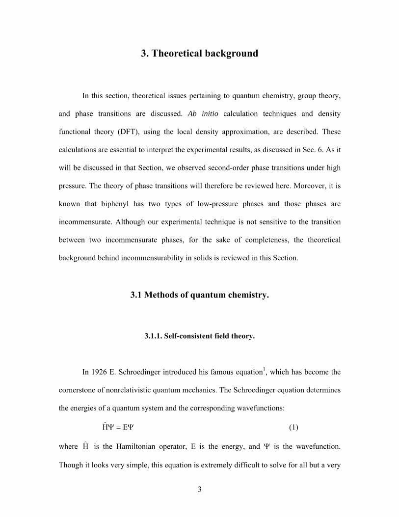
3. Theoretical background
In this section, theoretical issues pertaining to quantum chemistry, group theory,
and phase transitions are discussed. Ab initio calculation techniques and density
functional theory (DFT), using the local density approximation, are described. These
calculations are essential to interpret the experimental results, as discussed in Sec. 6. As it
will be discussed in that Section, we observed second-order phase transitions under high
pressure. The theory of phase transitions will therefore be reviewed here. Moreover, it is
known that biphenyl has two types of low-pressure phases and those phases are
incommensurate. Although our experimental technique is not sensitive to the transition
between two incommensurate phases, for the sake of completeness, the theoretical
background behind incommensurability in solids is reviewed in this Section.
3.1 Methods of quantum chemistry.
3.1.1. Self-consistent field theory.
In 1926 E. Schroedinger introduced his famous equation1, which has become the
cornerstone of nonrelativistic quantum mechanics. The Schroedinger equation determines
the energies of a quantum system and the corresponding wavefunctions:
Ψ=Ψ EH)
(1)
where H)
is the Hamiltonian operator, E is the energy, and Ψ is the wavefunction.
Though it looks very simple, this equation is extremely difficult to solve for all but a very
3

limited number of cases. In general, it is necessary to use approximations that enable one
to derive solutions to the Schroedinger equation.
In the general case, the Hamiltonian operator for an atom is given by:
∑∑≠ −
+⎟⎟⎠
⎞⎜⎜⎝
⎛+∆−=
ji jii ii rr
121
rZ
21H rr
), (2)
where atomic units are used throughout this chapter, Z is the charge of the atomic
nucleus, and is the radius-vector of the iirr th electron. The first two terms describe the
kinetic and potential energy of electrons in the field of the atomic nucleus, whereas the
last term describes the electron-electron interaction. It is this term that makes the equation
so hard to solve. Only the hydrogen atom can be solved exactly using the Schroedinger
equation—even for the helium atom one must use some approximations. The first
successful approach to solve the problem of atomic structure was made by Hartree2. The
Hartree method was later extended by Fock3 to take into account the Pauli exclusion
principle.
The Hartree approach is based on the variational principle, which states that for
the true ground-state wavefunction, the energy of the system is at its minimum. Thus
from the variational principle one can write for an arbitrary wavefunction , such that Ψ
12 =Ψ , that the following inequality holds:
ΨΨ≤ HE0 , (3)
where E0 is the ground-state energy. The equality occurs only for the true ground-state
wavefunction. Thus we can take a wavefunction, substitute it in (1), and find the
minimum with respect to wavefunction variation Ψδ . This procedure results in the
following equation:
4

0EH =ΨδΨ−ΨδΨ . (4)
Since Eq. (4) must be true for any arbitrary variation in wavefunction, one can write
0EH =Ψ−Ψ . (5)
In the Hartree method the wavefunction, which is the trial solution of Eq. (1), is
written as the product of one-electron wavefuctions:
)r()r()r( NN2211rrr
ψ⋅⋅⋅ψψ=Ψ , (6)
where N is the number of electrons. Let us take the helium atom as an example4. For the
ground state we choose:
2eff1eff rZ3effrZ
3eff
21 eZeZ)r,r( −−
ππ=ψ
rr , (7)
where Zeff is the effective charge of the atomic nucleus due to screening by the electrons.
Substituting Eq. (7) into Eq. (1) yields the energy as a function of Zeff. Minimizing that
expression with respect to Zeff yields the value of the effective charge Zeff and the ground-
state energy E. For the helium atom, the ground-state energy is given by:
effeff2eff Z
85ZZ2ZE +−= . (8)
The minimum occurs at Zeff=Z-5/16, which yields E=-2.85 a.u. (the experimental value is
-2.90).
The Hartree method does not take into account the exchange interaction between
electrons. This interaction is a result of the Pauli exclusion principle, which states that no
two fermions (e.g., electrons) can occupy the same quantum state. The Pauli principle is
accounted for in the Hartree-Fock (HF) approximation. This approach uses multielectron
wavefunctions in the form of a so-called Slater determinant:
5

),r(),r(
),r(),r(),r(),r(
!N1
NNN11N
112
NN1221111
σψ⋅⋅⋅σψ⋅⋅⋅⋅⋅⋅⋅⋅⋅⋅⋅⋅⋅⋅σψ
σψ⋅⋅σψσψ
=Ψ
rr
r
rrr
, (9)
where denotes the spin variable of the iiσ th electron. This wavefunction is constructed to
satisfy the Pauli principle. The HF method often gives very good results for atomic
ground-state energies.
Unfortunately, self-consistent HF equations also require much computational
effort to be solved, especially in the case of heavy atoms. In this case, there is another
approach that yields atomic parameters with fairly good accuracy. It is called the
Thomas-Fermi model.
3.1.2. Thomas-Fermi theory.
For heavy atoms one can use a quasiclassical approach and think of electrons as a
“gas” with a number density )r(nr
. The density of the electron gas is related to its Fermi
wave vector by4:
2
3F
3pnπ
= . (10)
In an electrostatic field, the energy of an electron can be represented as
ϕ−=2
pE2
, (11)
where ϕ is the potential. It is clear that E must be less than zero, otherwise the electron
would not be bound. Therefore one can write:
6
0
2F
2p
ϕ−ϕ= , (12)
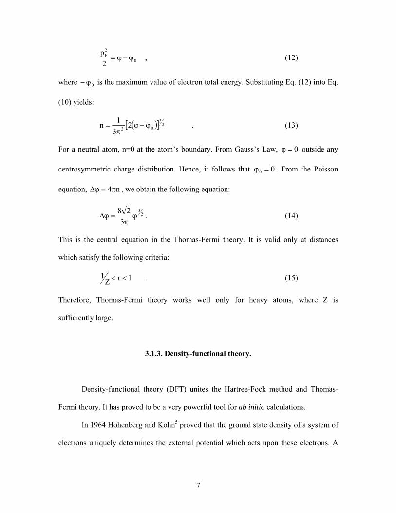
where is the maximum value of electron total energy. Substituting Eq. (12) into Eq.
(10) yields:
0ϕ−
( )[ ] 23
02 23
1n ϕ−ϕπ
= . (13)
For a neutral atom, n=0 at the atom’s boundary. From Gauss’s Law, outside any
centrosymmetric charge distribution. Hence, it follows that
0=ϕ
00 =ϕ . From the Poisson
equation, , we obtain the following equation: n4π=ϕ∆
23
328
ϕπ
=ϕ∆ . (14)
This is the central equation in the Thomas-Fermi theory. It is valid only at distances
which satisfy the following criteria:
1rZ1 << . (15)
Therefore, Thomas-Fermi theory works well only for heavy atoms, where Z is
sufficiently large.
3.1.3. Density-functional theory.
Density-functional theory (DFT) unites the Hartree-Fock method and Thomas-
Fermi theory. It has proved to be a very powerful tool for ab initio calculations.
In 1964 Hohenberg and Kohn5 proved that the ground state density of a system of
electrons uniquely determines the external potential which acts upon these electrons. A
7
proof by contradiction is outlined here. Suppose we have two distinct potentials )r(vr
and
)r(vr′ , such that const)r()r(v ≠v′−
rr. If we assume that both potentials give rise to the
same electron density )r(nr
, then we can write, using the minimum property of the ground
state Ψ :
( ) ( ) ( ) ( ) ( )( )rvrvrnErvrv ′−+′=Ψ′′−Ψ′
HHHErrrrr+Ψ′′Ψ′=Ψ′Ψ′<ΨΨ=
, (16)
H′ . where Ψ′ is the ground state wavefunction for Hamiltonian
Analogously we can obtain:
( ) ( ) ( ) ( ) ( )( vrvrnErvrv −′+=Ψ−′Ψ
By adding Eq. (16) and Eq. (17), it follows that EEE
)r
HHHErrrrr
+ΨΨ=Ψ′Ψ<Ψ′′Ψ′=′ . (17)
E<′+ +′ , which is impossible.
This pr
he electrons in an external potential
oves the central theorem of density functional theory.
For t )r(vr
the ground state energy can be
written as6,7
[ ]nGrdrdrr2 ′−
)r(n)r(n1rd)r(n)r(vE +′′
+= ∫∫rr
rr
rrrrr , (18)
where G is a functional of density
(19)
Then, using the fact that δ∫
, the exact form of which is unknown:
[ ] [ ] [ ]nEnTnG xcs +≡ ,
where [ ]nExc is the exchange-correlation functional.
rd)r(nrr
0= , one can obtain the following system of equations:
rd)r(v)r( rr)r(n rrrrr
r
′+=ϕ ∫ ′−′ (20)
8
[ ])r(n)r(n~xcxc )r(n~d/))r(n~E(d)n( rr
rr=
≡µ (21)
[ ] )r()r())r(n()r(21
iiixc2 rrrr
ψε=ψ⎭⎬⎫
⎩⎨⎧ µ+ϕ+∇− (22)
∑ ψ= 2i )r()r(n rr
(23) =
N
1i
The system (20)-(23) must be solved self-consistently. The energy is given by:
[ ] ∫ µ−+ d))r(n()r(n)r(nE xcxcrrr
It is necessary to emphasize that the energies
∫∫∑ ′−ε= ′−′
=
r
rdrd21E rr
)r(n)r(nN
1ii
r
rrrr
rr
(24)
iε and wavefunctions )r(r
ψ do not have
any physical meaning by themselves. Only the
i
electron density [Eq. (23)] and the energy
. of the system [Eq. (24)] have physical meaning6,7
Since the exact form of the functional ( ))r(nE xcr is unknown, an approximate
form must be used. Since the introduction of DFT, several approximations have been
developed. The most prominent and famous is the local density approximation (LDA),
which represents the exchange-correlation functional as:
[ ] ( )( ) ( ) rdrnrneEnE xcLDAxcxc
rrr∫=≈ (25)
where )n(exc is the exchange-correlation energy per particle in a uniform electron gas7.
This approximation in many cases turns out to work very well for determining
molecular structures. It also gives fairly good accuracy for ionization energies of atoms
and dissociation energies of molecules. Nevertheless, it fails in determining band gaps in
solids, heavy fermion systems, and other systems with strong electron-electron
interactions.
9

3.1.4. Molecular structure determination.
When two or more atoms come close together, their electronic clouds overlap and,
in certain cases, form a bond between the atoms. The Hamiltonian for this system
includes terms describing the interaction of nuclei with each other, as well as electrons
with not only their parent nuclei but also with all other nuclei in the molecule.
( )
∑∑∑∑
∑∑
≠= =≠ −−− ji ji
N
1i
M
1j ji
i
ji ji
ji 121ZZZ
21
rrrRR
==
+−
+∆−∆−=M
1i
N
1i iM1N1 2
1M21,,;,,H
ii
R
rrRR rR
rrrrrr
rK
rrK
rrr
ber of electrons; N is the number of nuclei; Zi is the charge and
i is t
(26)
Here M is the total num
M he mass of the ith nucleus; iRr
and jrr are radius-vectors of the ith nucleus and jth
electron, respectively.
We can significantly simplify the operator in Eq. (26), using the fact that the mass
of a nucleus is over a thousand times larger than the mass of an electron. Thus one can
neglect the kinetic energy of the nuclei, which is the first term in Eq. (26). All the nuclei
are assumed to be fixed in space, and the potential energy of their interaction with each
other is just an additive constant to the Hamiltonian, which can be added to the total
energy of the system. The Hamiltonian of the system is then given by:
( )
∑
∑∑∑
≠ −ji ji
121
rr
= ==
+
−−∆−=
N
1i
M
1j ji
iM
1iM1N1
Z21,,;,,H
i rRrrRR r
rr
rrr
Krr
Kr
r
Hamiltonian operator for the electronic coordinates only. The solution to the
(27)
This approximation is called the Born-Oppenheimer approximation. We are left with a
10
corresponding s theSchroedinger equation yield electronic wavefunction,
( )iM1 ;,, Rrrrr
Kr
Ψ , and the energy of the system, ( )iE Rr
, which depend parametrically
on the internuclear distances. The minimum of the energy with respect to the variation of
internuclear distances determines a possible stable structure of the molecule, and the
global minimum corresponds to the ground-state energy of the molecule. The nuclear
sidered as if all the nuclei moved in the potential
( ) ( )iN1 E,,U RRR =K . Energy levels for such a potential correspond to vibrational
levels of the mole
motion is then con
cule. A discussion of molecular vibrations will be given in the
llowing sections.
3.1.5. Group theory.
n, defined on this set such that all the elements of the set obey the following
postulates8:
1. two elements, a and b from A, the element c=ab belongs to
3. t e in A, such that ae=ea=a. This element is called
4. alled a-1, such that aa-1=a-1a=e.
fo
The set of elements A is called a group if there is an operation, which we will call
multiplicatio
For every
the set A.
2. The associative law of multiplication holds: abc=(ab)c=a(bc).
There is an elemen
the unity element.
For every a in A, there is an element, c
This element is called the inverse of a.
11
The multiplication operation does not necessarily mean ordinary multiplication. It
can be a combination of operations; for example, two differentiations. Examples of
groups include the set of all integers with respect to addition, the set of all rational
umbern s with respect to ordinary multiplication, and the set of n×n invertible matrices
with respect to matrix multiplication.
The importance of group theory to physics and chemistry is hard to overestimate.
Applying group-theoretical analysis, one can determine the vibrations that give rise to
infrared (IR) active modes and Raman active modes in the molecular spectra, determine
the degeneracy of molecular energy levels, and so on.
When dealing with a particular molecule, one can perform a number of operations
on it; namely, rotation about given axis, reflection about a given plane, inversion, or a
combination of rotation and inversion. It is clear that only rotations by the angle n2π ,
where n is an integer, form a group of rotations*. The axis of rotation is called the axis of
nth order and is denoted as Cn. If the symmetry operations involve a rotation plus
inversion operation, then the axis is denoted as Sn. The main axis of rotation is the axis of
the highest order. The plane of reflection is marked as σ and is given the subscript v or h,
depending on whether the plane contains the main axis of rotation or is perpendicular to
it, resp
ectively. Thus if the plane contains the main axis, it is σv, and if the plane is
perpendicular to it, it is the σh plane. The inversion operation is denoted by the symbol i.
* If electrons are considered, the rotations by n
4π form a group of rotations, due to electron spin.
12
It is straightforward cribed above leave at least
ne point of the molecule unmoved in space. Therefore such a group of operations is
called a point group. In the following sections, several specific examples are described.
to verify that all the operations des
o
3.1.6. Examples of point groups.
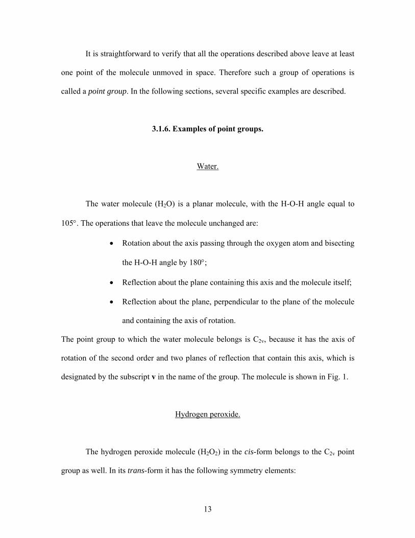
Water.
The wa
105°. The oper o
• ugh the oxygen atom and bisecting
and containing the axis of rotation.
The point group to which the wa is C2v, because it has the axis of
rotation of the second order and two planes f reflection that contain this axis, which is
peroxide.
ter molecule (H2O) is a planar molecule, with the H-O-H angle equal to
ati ns that leave the molecule unchanged are:
Rotation about the axis passing thro
the H-O-H angle by 180°;
• Reflection about the plane containing this axis and the molecule itself;
• Reflection about the plane, perpendicular to the plane of the molecule
ter molecule belongs
o
designated by the subscript v in the name of the group. The molecule is shown in Fig. 1.
Hydrogen
The hydrogen peroxide molecule (H2O2) in the cis-form belongs to the C2v point
group as well. I t
n i s trans-form it has the following symmetry elements:
13

• The center of inversion;
• The axis of rotation of the second order, which is perpendicular to the
molecule plane;
• The plane of reflection that coincides with the plane of the molecule.
Because the plane of reflection is perp o the main axis of rotation, the point
group of this molecule is C2h. Again, the subscript h denotes the fact that the main axis
endicular t
and the plane of symmetry are orthogonal. The molecule is shown in Fig. 2.
Benzene.
The be n
• lar to the molecule plane;
•
• 6 axes of rotation of the second order, which are the lines of
intersection of the plane of the molecule and 6 planes of reflection.
ecause of these second-order rotational axes, the group is labeled by the symbol D.
Finally, the point group of the benzene molecule is D6h. The molecule is shown in Fig. 3.
nze e molecule (C6H6) has the following symmetry elements:
The main axis of 6th order, perpendicu
• The plane of reflection, which coincides with the molecule plane;
The center of inversion;
• 6 planes of reflection containing the main axis of symmetry and being
perpendicular to the molecule plane;
B
14

Figure 1. Water molecule.
Figure 2. Hydrogen peroxide molecule.
Figure 3. Benzene molecule.
15

3.1.7. Mathematical background.
In order to describe a symmetry operation, denoted as R , we can use the
coordinate system in real space and represent any operation as a transfo ation of the
radius-vector r
rmr
. It is well known that the transformation of any vector into another vector
can be perfo d by a matrix T. Every symmetry operation can therefore be described by r
a matrix, reducing the grou es is
of matrices can be obtained from another
me
p theory to the algebra of matrices. Such a set of matric
said to form a representation of the group. We will use the symbol Γ to denote a
particular representation. There are many possible representati ons of the group. If one set
B A by the rule
ch that for any matrix from the set
QAQB 1−= , (28)
then these two representations are said to be equivalent. Equation (28) states that there is
an invertible matrix Q su A there is a matrix in the
t
lar representation is called the character of the representation.
s of a point group, characters form a table of
characters, which completely describes the group. The Great Orthogonality Theorem
se that can be obtained by a unitary transformation. If the matrices of the given
representation can be simultaneously broken into block-diagonal form, the representation
is called reducible. Otherwise it is called irreducible, and these are the representations
that are of interest to us.
The trace of a matrix of a given operation is called the character of this operation.
It is denoted by the symbol χ, so that χ(R) is the character of the operation R. The set of
all characters for a particu
B
In the case of irreducible representation
16

holds f uc le
can be lsewh
heorem:
If and
or s h a tab of characters. We provide its formulation without proof here, which
found e ere8.
Great Orthogonality T
µΓ νΓ are two non-equivalent irr
and of dimensions and respectively, then the matrix elements
are related by the equation
educible representations with matrices
)(D Rµ )(D Rνµn νn ,
( ) kmijmjik µνµR
where g is the order of the group and the sum is over
1 ng)(D)(D δδδ=−νµ∑ RR (29)
all the operations R. With the help
of this theorem, it is possible to expa le representation into a sum of
irreducible re ext section it
is used to solve the problem of molecular vibrations.
ts. Some of these displacements, however, will involve motion in which no
bond length or bond angle changes. Those displacements correspond to translation along,
and rotation about, three non-coplanar axes. The Hamiltonian of the system can be
nd any reducib
presentations. This theorem has many applications, and in the n
3.1.8. Application of group theory to molecular vibrations.
For a molecule consisting of N atoms, there are 3N possible atomic
displacemen
written as:
( ) ( )N321
N3
1i i
2i
N321 x,,x,xWM2px,,x,xH KK += ∑
=
, (30)
where W is the potential energy of the N nuclei. The potential can be expanded around
the equilibrium as follows:
17
( )
( ) ( )( ) L+−−∂
K
∂∂
+−∂∂
+=
∑ ∑∑0
N3 N3 N3
ii
0N321
21xx
xW
Wx,,x,xW
= = =00 jjii
1i 1i 1j ji
2
i
xxxxxx
W (31)
The constant factor W0 can be set to zero. In addition, at equilibrium, all first derivatives
vanish. Thus we obtain the Hamiltonian:
( )
( )( ) L= =1i 1j ji
N3 2ip
(32)
Restricting the expansion to the quadratic terms, we obtain the harmonic approximation.
Second derivatives of the potential energy are called harm acing
by qi, displacement from equilibrium for the ith coordinate, yields:
K
+−−∂∂
∂
+=
∑∑
∑=
N3
jjii
N3 2
1i iN321
00xxxx
xxW
21
M2x,,x,xW
onic force constants. Repl
0ii xx −
( ) ∑∑∑= ==
+=N3
1i
N3
1jjiij
N3
1i i
2i
N321 qqB21
M2pq,,q,qH K , (33)
whereji
2
ij xxWB∂∂
∂=
diagonalizes the ma
. One can find a linear transformation of coordinates qi that
trix ijB . The Hamiltonian is then expressed as:
( ) ∑∑ ξ+=ξξξN3
2ii
N3 2i
N321 k1p,,,H K , (34) == 1i1i i 2M2
where ξi are the new coordinates, called normal coordinates. The coefficients ki are
ordinary force constants for the harmonic oscillator. Since six modes correspond to
translational and rotational motion, exactly six coefficients ki will be equal to zero.
Excluding those coefficients from consideration, we r the can write the Hamiltonian fo
vibrational problem:
18

( ) ∑∑6N3
1i
26N3
1i i
2i k
21
M2pH
−
=
−
=
ξ+=ξξξ ,,, (35)
Since any symmetry operation leaves the molecule unchanged, th
ii6N321 −K
e Hamiltonian is
reserved under symmetry operations. It is known that every normal coordinate belongs
to an irreducible representation of corresponding harmonic-oscillator
wavefunctions (1st excited state) belong to the same representation. A group-theoretical
alysi
Exam
p
the group. The
an s is used to determine the modes which are IR- or Raman active.
ple: H2O.
ter molecule. It belongs to the C2v point group.
The table of characters is given as follows8:
C v σ σ
As an example, consider the wa
2 E C2(z) xz yz
A1 1 1 1 1
A2 1 1 -1 -1
B1 1 -1 1 -1
B2 1 -1 -1 1
siteΓ 3 1 1 3
RrΓ 3 -1 1 1
N3Γ 9 -1 1 3
take the direct product of two representations: for the radius-vector
In order to obtain the representation for 3N atomic displacements, Γ , we must N3
Rr
, RrΓ , and for the
19
atomic sites siteΓ . The representation for the radius-vector is, in turn, the direct product of
the representations of x-, y-, and z-components. In our case these are A2, B1, and B2
representations. The character of a given transformation for the siteΓ representation is
equal to the nu that remain stationary under this transformation. The results mber of atoms
for two representations (radius-vector and sites) are listed in table of characters. The last
line represents the characters for the represen the tation with atomic displacements as
basis, where siteN3 Γ⊗Γ=Γ Rr . Using the Great Orthogonality Theorem we can expand
N3Γ :
B3B2AA3 21N3 21 ⊕⊕⊕=Γ (36)
As was mentioned before, there are six modes which are rotational or translational
modes. We must exclude tho 1, B1,
2
r mode. In addition there is
1
2
se from Eq. (36). Three translations correspond to A
and B representations respectively. Three rotations correspond to A2, B1, and B2
representations. Subtracting those six modes from Eq. (36) yields:
21N3 BA2 ⊕=Γ (37)
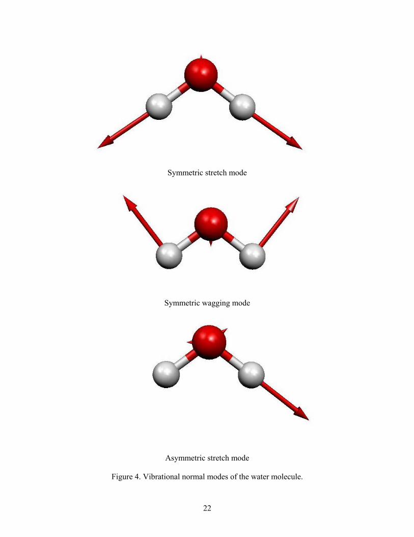
Considering the water molecule qualitatively, there are symmetric modes, with
hydrogen atoms moving along the O-H bonds for one mode and with H-O-H angle
oscillating around its equilibrium value (Fig. 4) for the othe
one asymmetric mode, where the hydrogen atoms move along the bonds, out of phase
with the oxygen atom (Fig. 4). The two symmetric modes belong to the A representation
and the asymmetric one belongs to the B representation.
Now we may ask the question: which modes are IR-active and which are not? IR-
activity means that if we shine light onto the system, the mode absorbs energy and
becomes excited. The transmitted light intensity at the frequency corresponding to this
20

mode decreases. For a mode to be IR-active, it must have a nonzero dipole moment
induced (Appendix A). For the water molecule, the answer is evident from Figure 1. The
two symmetric modes produce a dipole moment along the z-axis (which is also the main
be used to unambiguously determine the IR activity of
vibrational modes. In order for the m
probability for the transition from the ground state to this particular excited state. The
transition rate is given by:
axis of symmetry), and the asymmetric mode produces a dipole moment in the plane of
the molecule perpendicular to the main axis. Thus, for the water molecule, all three
modes should be IR-active. In fact, it is known from experiments that this is the case.
Group theory can
ode to become excited, there must be a nonzero
2
a0a0 dP ∫ ττψτψ∝ )()( dr
, (38)
here w 0ψ and aψ are wavefunctions of the ground state and the excited state,
respectively, and d is the dipole moment. The set of all arguments, on which the
wavefunctions depend, is labeled
r
τ .
The integral in Eq. (38) will be zero if the integrand is an odd function. The
wavefunction of the ground sta always belongs to the totally symmte etric representation
(A1 in the case of the water molecule). Thus integral in (38) is zero unless belongs to
e
aψ
the sam representation as the dipole moment. The dipole moment has the same
symmetry as the radius-vector Rr
. In the case of the water molecule,
211 BBA ⊕⊕=ΓRr
Hence, must belong to the A1, B1, or B2 representation. From Eq. (37), it is apparent
that all three modes are IR-active.
aψ
21
Symmetric stretch mode
Symmetric wagging mode
Asymmetric stretch mode
Figure 4. Vibrational normal modes of the water molecule.
22
3.2. Numerical calculations.
As it was seen in the previous sections, in order to determine a molecular
structure we must solve the Schroedinger equation with a Hamiltonian given by Eq. (27).
The computational resources required to solve this equation grow rapidly with the
number of electrons. In order to apply any of the available numerical methods, we must
limit the number of electrons taken into account. It is known that usually only the outer
electrons are involved in bond formation. To first order, the inner-shell electrons can be
ignored. This approximation greatly reduces the number of basis wavefunctions involved
in the calculation.
In any numerical method of solving the Schroedinger equation, the one-electron
wavefunctions are expanded in terms of certain basis functions, which are usually chosen
to be orthonormal. This significantly reduces the computational cost of solving all the
equations.
Currently there are commercially available software packages which perform the
task of calculating molecular structures. In this work, the Gaussian98 program (Ref. 9)
has been used. It has many built-in methods, including Hartree-Fock and DFT, and uses a
variety of basis sets. All the basis sets include Gaussian-type functions; i.e., functions that
look like9:
( ) 2rlmn zycxg α−=α e,rr , (39)
where x, y, and z are components of the radius-vector rr
and c is the normalization
constant. All such functions are normalized to unity:
23

1gspaceall
2 =∫ (40)
The list of different basis sets used by Gaussian program is given in Table I:
Table I. Description of the basis sets used by GAUSSIAN program.
# Basis Functions Basis set [Applicable atoms]
Description 1st row
atoms hydrogen
atoms STO-3G [H-Xe]
Minimal basis set: use for more qualitative results on very large systems. 5 1
3-21G [H-Xe]
Split valence: 2 sets of functions in the valence region provide a more accurate
representation of orbitals. 9 2
6-31G(d), 6-31G* [H-Cl]
Adds polarization functions to heavy atoms. (This basis set uses the 6-
component type d-functions.) 15 2
6-31G(d,p), 6-31G** [H-Cl]
Adds polarization functions to the hydrogens too. 15 5
6-31+G(d) [H-Cl]
Adds diffuse functions: important for systems with lone pairs, anions, excited
states. 19 2
6-31+G(d,p) [H-Cl]
Adds p-functions to hydrogens as well. 19 5
6-311+G(d,p) [H-Br]
Triple zeta: adds extra valence functions (3 sizes of s and p functions) to 6-
31+G(d).Diffuse functions can be added to the hydrogen atoms via a second +.
22 6
6-311+G(2d,p) [H-Br]
Puts 2d functions on heavy atoms (plus diffuse functions), and 1p function on
hydrogens. 27 6
6-311+G(2df,2p) [H-Br]
Puts 2d functions and 1f function on heavy atoms (plus diffuse functions), and
2p functions on the hydrogen atoms. 34 9
6-311+G(3df,2pd) [H-Br]
Puts 3d functions and 1f function on heavy atoms, and 2p functions and 1d
function on hydrogens, as well as diffuse functions on both.
39 15
24

3.3. Theory of phase transitions.
In the present work, we observed second-order phase transitions in conjugated
organic solids under high pressure. It is therefore necessary to discuss the theory behind
those phenomena. It is also known that biphenyl has two low-pressure phases which are
incommensurate. Although our experimental methods are not sensitive to
incommensurate-incommensurate phase transitions, the issues related to incommensurate
phases are briefly discussed.
3.3.1 General properties of phase transitions.
When two or more macroscopically distinguishable substances are located in a
given system, it is said that the system consists of several phases. Examples of such
systems include ice-water (solid-liquid system), mercury-water (two immiscible liquids),
and water-air (liquid-gas system) mixtures. In all multiphase systems, different phases are
separated by interfaces such that they are macroscopically distinct. When a chemically
homogeneous material melts, evaporates, or undergoes some other structural
transformation, it is said to undergo a phase transition.
During any phase transition, the thermodynamic potential per unit volume
remains continuous with variations in temperature and pressure. Therefore, the condition
for the phase transition to occur is such that specific thermodynamic potentials of two
phases, and , are equal1Ψ 2Ψ 10:
( ) ( TPTP 21 ,, Ψ=Ψ ) , (41)
25

where P is pressure and T is temperature. Eq. (41) determines not just one point but rather
a phase-transition line on the P-T diagram. For each point on this line, the two phases are
in equilibrium with each other and can coexist in the system. On the side where 21 Ψ>Ψ ,
phase 2 is more stable, and on the other side, phase 1 is more stable.
If there are more than two phases for a given substance, there is a possibility of
the coexistence of more than two phases. In this case the following condition must be
satisfied:
( ) ( ) ( ) ( )( ) ( ) ( ) ( )TPTPTPTP
TPTPTPTP
1nn1n
3221
,,;,,;;,,;,,
Ψ=ΨΨ=ΨΨ=ΨΨ=Ψ
−
L (42)
where n is the total number of phases. From this equation it is clearly seen that three
phases can coexist only at one point on P-T diagram. This point is called the triple point.
It is also evident that for more than three phases, Eq. (42) can be satisfied only by
accident. This means that, in general, more than three phases of the same material cannot
coexist simultaneously.
As stated earlier, the specific thermodynamic potential for the material remains
continuous throughout phase transformations. Its derivatives, however, can be
discontinuous. Usually, phase transitions are divided into two types: first-order phase
transitions and second-order phase transitions, depending on the properties of the first-
and second-order derivatives of the thermodynamic potential.
26

3.3.2. First-order phase transitions.
In first-order phase transitions, the first derivatives of the thermodynamic
potential are discontinuous. From the definition of Ψ Ψ , it is known that sT
−=∂Ψ∂ and
vP
=∂Ψ∂ , where s and are the specific entropy and volume, respectively. Thus, either
the specific entropy or specific volume of the substance, or both, exhibits a discontinuity
upon the phase transition. The change in specific entropy is associated with the latent
heat of the phase transition. It is this heat that is required to melt ice or boil a teapot.
From the expansion of near the phase equilibrium, and condition (41), the
following relationship can be derived:
v
( TP,Ψ )
( )1212
12
vvTq
vvss
dTdP
−=
−−
= , (43)
where q is the heat required to transform phase 2 into phase 1. Eq. (43), known as the
Clapeyron equation, defines the slope of the coexistence curve on the P-T diagram.
3.3.3. Second-order phase transitions.
Another type of phase transition is characterized by discontinuities in the second-
order derivatives of the thermodynamic potential, while the first-order derivatives remain
continuous. This means that during a second-order phase transition, the specific volume
of the substance does not change, and no heat is added to or withdrawn from the system.
At the same time, quantities such as the specific heat, bulk modulus, and thermal
27
expansion coefficient are discontinuous. Examples include the ferromagnetic-
paramagnetic phase transition, Bose-Einstein condensation, and the conductor-
superconductor transition.
In the case of ferromagnetic systems, such as iron or nickel, the material has a
nonzero magnetic moment in the ferromagnetic phase. When the substance is heated
above a certain temperature Tc, the magnetic moment becomes zero. This temperature is
called the Curie temperature or critical temperature. The appearance of spontaneous
magnetization below the critical temperature is the result of a second-order phase
transition.
It is immediately evident that the paramagnetic phase and ferromagnetic phase
possess different symmetries. In the paramagnetic phase, for an isotropic medium, the
system is invariant under any rotation in space. In the ferromagnetic phase, the magnetic
moment marks the preferred direction in space and the system is invariant only under
rotations about this direction. The symmetry is therefore reduced. The phenomenon of
symmetry reduction is a feature of all second-order phase transitions. In such a phase
transition, the symmetry is said to be spontaneously broken.
Since one of the phases has lower symmetry, it requires more parameters to be
described than the highly symmetric phase. The extra parameter that is necessary for such
a description is called the order parameter. The order parameter is zero in the highly
symmetric phase and becomes nonzero upon the phase transition. In the case of the
ferromagnetic transition, it is magnetization that serves as the order parameter. The order
parameter is measurable in the experiment and is the extensive thermodynamic variable.
28

Usually, the order parameter is associated with some intensive variable, which is
conjugate to it. In the present example, the intensive variable is the magnetic field.
3.3.4. Landau theory of second-order phase transitions.
During second-order phase transitions, the thermodynamic potential is a
continuous function of the intensive variables and so are its first-order derivatives. In the
low-symmetry phase, the order parameter is nonzero and becomes zero upon the phase
transition. It is natural to assume that near the phase transition point, the order parameter
is the only parameter that is important. The thermodynamic potential can be expanded in
powers of the order parameter10,11:
( ) LL +η∇++η+η+η+η−Ψ=ηΨ 242
31
200 2
caaaH (44)
where η is the order parameter and H is the conjugated field. The last term in Eq. (44) is
added in order to take into account the spatial variations in the order parameter. The
importance of this term will be clarified in the sections that follow.
If the system properties are symmetric under reversal of η, then a1=0. It is also
assumed that , wheretra 00 =c
c
TTT
t−
= . Thus, in the absence of an external field, the
thermodynamic potential above Tc has its minimum at η=0, whereas below the Tc there is
a nontrivial value of the order parameter corresponding to the minimum in . Ψ
Landau theory deals only with quantities that are of macroscopic nature. It also
ignores all fluctuations. In the simplest case, one can assume that the order parameter is
29
independent of position and restrict the series to the quartic terms. Then Eq. (44) reduces
to:
( ) 42
200 atrH η+η+η−Ψ=ηΨ . (45)
In order for the thermodynamic potential to be at a minimum, the following two
conditions must be satisfied:
0
0
2
2
≥η∂Ψ∂
=η∂Ψ∂
. (46)
Substituting Eq. (45) into these two conditions yields:
0a12tr2
0Ha4tr22020
30200
≥η+
=−η+η . (47)
In the absence of an external field (H=0), for the case t>0, the only real solution is
. When t<0, the solution is given by: 00 =η
ta2r
2
00 =η . (48)
The generalized susceptibility is determined as χ0
HH 2
2
η=η∂η∂
=∂
Ψ∂−=χ . From Eqs. (47)
and (48) one can obtain:
⎪⎪⎩
⎪⎪⎨
⎧
<−
>
=χ0t
tr41
0ttr2
1
0
0 (49)
This is known as the Curie-Weiss law.
30

The last result we are interested in is the dependence of the order parameter on the
external field. From Eq. (47), the order parameter at t=0 is
32
0 a4H=η . (50)
The specific heat is given by:
⎩⎨⎧
<
>=
0ta8kTr30t0
C2
2c
20 ,
, (51)
It is apparent that at the critical temperature, second-order derivatives of the
thermodynamic potential are discontinuous. Moreover, the susceptibility diverges as t1 .
Since this derivation was done without specifying the nature of H and η, these results can
be generalized for every second-order phase transition considered within the framework
of Landau theory.
It turns out that it is fluctuations that lead to the occurrence of the phase transition.
As was mentioned before, Landau theory does not take into account such fluctuations.
Nonetheless, the general idea about the divergence in second-order derivatives of the
thermodynamic potential remains valid. The dependence of thermodynamic quantities
upon value of t can be expressed as follows:
( )ν−
δ
γ−
β
α−
∝ξ
=∝η
∝χ
∝η
∝
t
0tH
t
t
tC
1
. (52)
The parameters α, β, γ, δ, and ν are called critical exponents, and ξ is the correlation
length. The critical exponents show great degree of universality, being the same for quite
31

different systems. In renormalization group theory, all phenomena are divided into
universality classes depending on the values of the critical exponents.
In the present example the critical exponents are given by:
32112
10 =δ=ν=γ=β=α ;;;;
3.2.5. Correlation function.
In the present section, the correlation function is related to the correlation length.
A correlation function can be evaluated in the framework of Landau theory using the
fluctuation-dissipation theorem (FDT). The correlation function is defined as:
( ) ( ) ( )[ ] ( ) ( )[ ]rrrrrr ′η−′ηη−η=′ rrrrrr,g (53)
The fluctuation-dissipation theorem11 states that:
( ) ( ) (∫ ′δ′′=ηδ rrrrr rrrrr HgdTk
1
B
, ) (54)
if ( )rr
η and are conjugate parameters. Using the most general form of expansion
given in Eq. (44), we obtain the following equation for correlation function:
( )rrH
( )[ ] ( ) ( )rrrrr rrrrr ′−δ=′∇−η+ Tkgca12tr2 B22
20 , (55)
In the absence of an external field, the average value of the order parameter is given by
Eq. (48) for t<0 and is zero for t>0. The solution for Eq. (55) in three dimensions is given
by:
( ) ( )c4Tkexp
,g B
π′−
ξ′−−=′
rrrr
rr rr
rrrr , (56)
where ξ takes the form:
32

( )( )⎪⎩
⎪⎨⎧
<−
>=ξ
−
−
0ttr2
0ttr
21
0
21
0 . (57)
Generally the correlation function is written in the so-called Ornstein-Zernike form12:
( ) ( )p
exp,g
rr
rrrr rr
rrrr
′−
ξ′−−∝′ , (58)
where ζ+−= 2dp ; d is the dimensionality of the system. Parameter ζ is another
critical exponent and in three dimensions 0=ζ .
3.2.6. Scaling hypothesis.
Since the nature of the order parameter in Landau theory was not specified, it
must give the same critical exponents for all second-order phase transitions. This
property is called universality. At the same time, it is now widely accepted that the
fluctuations near the critical point provide the main mechanism for the second-order
phase transitions, which Landau theory does not take into account. As the system
approaches the critical point, the fluctuations grow larger and approach a macroscopic
size. The hypothesis was made that in the vicinity of the critical point, the only relevant
parameter is the correlation length, which describes the size of the fluctuations13. Then it
follows that only two of the critical exponents are independent. The other exponents can
be expressed in terms of these two, and such expressions are called “scaling laws”:
( )
( ) lawWidom1lawRushbrooke22
lawJosephson2lawFisherd2
−δβ=γ=γ+β+α
ζ−ν=γν=α−
(59)
33
At the critical point, the correlation length diverges and there is no characteristic
distance relevant to the system. Suppose we take our system and divide it into cells in
such a way that the size of a cell is much less than the correlation length near the critical
point but much greater than the interparticle distance. In other words, , where a is
the interparticle distance and L is the cell size. Since the correlation length is the only
important parameter, we can average all microscopic variables over any cell and obtain
the same pattern as we had for original system. In other words, if we enlarge a given cell
to the size of the system, it would resemble the whole system. The value
ξ⟨⟨⟨⟨La
aLb = is then
called the rescaling factor. The parameters t and H are the only two that can change
upon rescaling. We may write the transformation rule for these two variables:
tbtHbH
y
x
=
=~
~ (60)
All critical exponents can be expressed in terms of x and y. For the correlation
length it immediately follows that y1=ν . From Eq. (58) it follows that the correlation
function scales as . Since the correlation function has the same dimension as ,
we can conclude that scales as
ζ−−d2b 2η
η ( ) 2d2b ζ−− . At the same time, since the order parameter is
given by H∂ϕ∂
=η , it scales as . Combining these two facts together, we obtain: dxb −
x2d2 −+=ζ . Now, using these expressions for ν and ζ , we can obtain all other
critical exponents. Altogether, we obtain:
34
x2d2xd
xy
dx2y
xdy
d2
y1
−+=ζ−
=δ
−=γ
−=β
−=α
=ν
. (61)
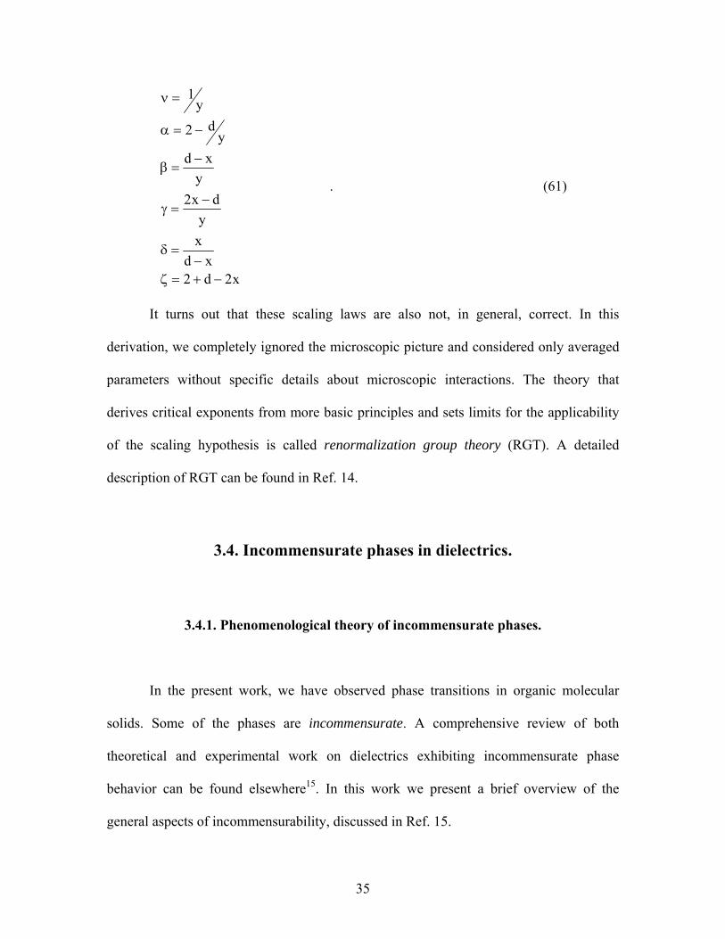
It turns out that these scaling laws are also not, in general, correct. In this
derivation, we completely ignored the microscopic picture and considered only averaged
parameters without specific details about microscopic interactions. The theory that
derives critical exponents from more basic principles and sets limits for the applicability
of the scaling hypothesis is called renormalization group theory (RGT). A detailed
description of RGT can be found in Ref. 14.
3.4. Incommensurate phases in dielectrics.
3.4.1. Phenomenological theory of incommensurate phases.
In the present work, we have observed phase transitions in organic molecular
solids. Some of the phases are incommensurate. A comprehensive review of both
theoretical and experimental work on dielectrics exhibiting incommensurate phase
behavior can be found elsewhere15. In this work we present a brief overview of the
general aspects of incommensurability, discussed in Ref. 15.
35

It is now generally accepted that an incommensurate phase is characterized by a
lack of translational periodicity in at least one direction. However, this phase has three-
dimensional long-range order, contrary to amorphous substances. In practice this means
that the ratio of the periodicity of some order parameter (e.g., polarization or chemical
composition) to the lattice periodicity is not a rational number. Incommensurate phases
exhibit several interesting phenomena—nonlinear multi-soliton lattice-type ground state,
phason excitation, devil’s staircase, solid-state chaos, etc.—that are not found in
translationally periodic systems.
In the simplest case the thermodynamic potential can be written as:
2
2
2242
0 dxd
2D
dxd
2C
4B
2tA
⎟⎟⎠
⎞⎜⎜⎝
⎛ η+⎟
⎠⎞
⎜⎝⎛ η
+η+η′
+Ψ=Ψ (62)
The incommensurate modulation is in the x-direction. In Fourier form Eq. (62) becomes:
( )
∑
∑
−−−
−
ηηηη+
ηη++′+Ψ=Ψ
321
321321kkk
kkkkkk
kkk
420
B41
DkCktA21
,,
~~
(63)
At the transition to the incommensurate phase, the function ( ) 42 DkCktAkA ++′=~
vanishes. Its minimum is located at the point D2Ck 2
0 −= . Thus the temperature of the
incommensurate phase transition is defined by:
( ) 0kA 0 =~ , (64)
which yields
⎟⎟⎠
⎞⎜⎜⎝
⎛′
+=AD4
C1TT2
ci . (65)
36

Other extrema for the functional (63) exist at k=0. They correspond to either the normal
(highly symmetric) phase or commensurate low-symmetric phase. In the commensurate
phase, and Eq. (63) becomes: ( ) constx =η
B4tA 22
0′
−Ψ=Ψ ~~ (66)
At the same time in the incommensurate phase we have (keeping only terms containing
): 00 kk −ηη
( ) ( )
i
0000
TT
22
0I
2kkkk00
B6tA
B23kA
=
−−
′−Ψ=Ψ
ηη+ηη+Ψ=Ψ
~~
~~
min
(67)
When the thermodynamic potentials become equal, the system “locks” itself in the
commensurate phase. The temperature of such “lock-in” transition is:
( )⎥⎦
⎤⎢⎣
⎡′+
−=AD4
26C1TT2
cl (68)
In the example considered above, we have a one-component order parameter. Let
us consider the more general case of the transition from one crystal lattice type into
another. Our discussion now will follow that in Ref. 10. The crystal can be characterized
by the electron density , which changes upon the phase transition. The symmetry of
the crystal poses some restrictions on the function
( )rr
ρ
( )rr
ρ ; namely, ( )rr
ρ should remain
invariant under all symmetry transformations of the crystal space group. Thus we can
always represent the density as a linear combination of the functions : )n(iφ
( ) ( )∑∑ φη=ρn i
ni
ni , (69)
37

where n denotes the number of the irreducible representation, i is the number of the
function in the basis for that representation.
The unit representation leaves all the functions invariant under all transformations
and represents, therefore, the high-symmetry phase. Eq. (69) can be written as:
( ) ( )∑ ∑ φη+ρ=δρ+ρ=ρn i
ni
ni00
' , (70)
where the prime indicates that the unit representation is excluded from the sum. At the
transition point all the coefficients iη must be zero. Therefore, the thermodynamic
potential can be expanded near the phase transition point in powers of iη . Since the
thermodynamic potential must not depend on the coordinate system, it has to contain only
the combination of , which is invariant under group symmetry transformations. The
linear invariant does not exist, therefore, to lowest order, this expansion is given by
iη
( ) ( ) ( )( )∑ ∑ η+Ψ=Ψn i
2ni
n0 TPA ,' . (71)
At the transition point, all A(n) values must be nonnegative in order for the
potential to be minimal. At the same time, at least one of the A(n) values must change sign
upon moving through the critical point, otherwise there would be no transition. For
simplicity we can assume that only one coefficient A(n), corresponding to nth irreducible
representation, changes sign. The coefficients iη , belonging to the same representation,
also become nonzero. This means that the symmetry reduces upon the transition, so that
the group of symmetry of the crystal below the transition point is the subgroup of the
group of symmetry above the critical point. Since only nth representation is important,
the superscript n can be omitted and coefficients iλ can be introduced as follows:
38

iii
2i
2 ; ηλ=ηη=η ∑ (72)
where is the “order parameter”, analogous to the one introduced earlier [see Eq. (44)].
It gives the quantitative measure of the deviation from the high-symmetry phase. The set
of coefficients represents the structure and the symmetry of the distorted (usually low-
symmetry) phase. The expansion of the thermodynamic potential can be represented as
follows:
η
iλ
( ) ( ) ( ) ( ) L+λη+η+Ψ=Ψ ∑j
i4
jj42
0 fTPCTPA ,, (73)
where is the invariant of the fourth order that can be constructed from the
coefficients . The sum over j extends over all possible invariants of the fourth order. At
the transition point, the coefficient A must be zero. The set of all
( ) ( )i4
jf λ
iλ
iη plays the role of the
order parameter in this theory.
In the case of two-dimensional order parameter, we must also include in Eq. (73)
the invariants constructed from the derivatives of iη . The expansion must contain terms
proportional to 2iη∇ , as well as terms of the form
xxi
kk
i ∂η∂
η−∂η∂
η for certain
symmetry groups. The requirement on these antisymmetric combinations is that one can
not construct vector components from those quantities. The term, containing those
antisymmetric combinations is called the Lifshitz invariant. The presence of the Lifshitz
invariant introduces spatial inhomogeneity and this is what is now called the
incommensurate phase. With the Lifshitz invariant, the consideration and all general
results remain the same.
39
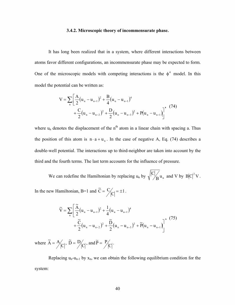
3.4.2. Microscopic theory of incommensurate phase.
It has long been realized that in a system, where different interactions between
atoms favor different configurations, an incommensurate phase may be expected to form.
One of the microscopic models with competing interactions is the model. In this
model the potential can be written as:
4φ
( ) ( )
( ) ( ) ( ⎥⎦⎤−+−+−+
⎢⎣⎡ −+−=
−−−
−−∑
1nn2
3nn2
2nn
n
41nn
21nn
uuPuu2Duu
2C
uu4Buu
2AV
), (74)
where un denotes the displacement of the nth atom in a linear chain with spacing a. Thus
the position of this atom is nuan +⋅ . In the case of negative A, Eq. (74) describes a
double-well potential. The interactions up to third-neighbor are taken into account by the
third and the fourth terms. The last term accounts for the influence of pressure.
We can redefine the Hamiltonian by replacing un by nuBC and V by VCB 2 .
In the new Hamiltonian, B=1 and 1CCC ±==~ .
( ) ( )
( ) ( ) ( ⎥⎦
⎤−+−+−+
⎢⎣
⎡−+−=
−−−
−−∑
1nn2
3nn2
2nn
n
41nn
21nn
uuPuu2Duu
2C
uu41uu
2AV
~~~)
~~
, (75)
where CAA =~ , C
DD =~ , and CPP~ = .
Replacing un-un-1 by xn, we can obtain the following equilibrium condition for the
system:
40

( ) ( )( )( ) constxxD~
xxD~2C~xxD~3C~2A~
2n2n
1n1n3nn
=+
+++++++
+−
+− (76)
Apart from the trivial solution ( 0x n = ) one can obtain two more solutions:
( )D~9C~4A~,x 2n ++−== ll (77)
and
( ) ( )D~A~,1x 2nn +−=−= ll (78)
The stability of all possible equilibrium configurations depends on the sign of the second
derivative. The stability condition implies that the eigenvalues of the matrix
0xxmn
2
nm xxV
=∂∂
∂=Ω
at the equilibrium configuration x0 are non-negative. For the trivial solution, the
eigenvalue equation is given by:
⎥⎥⎦
⎤
⎢⎢⎣
⎡⎟⎟⎠
⎞⎜⎜⎝
⎛−⎟
⎠⎞
⎜⎝⎛+⎟
⎠⎞
⎜⎝⎛+⎟
⎠⎞
⎜⎝⎛=ω
22222 1k
21cos4Dk
21cosC4Ak
21sinm (79)
It is clear that for arbitrary values of parameters, the right-hand side of Eq. (79) can
become negative. In that case, the trivial solution loses stability, which means that the
system transforms into another stable state. The critical wave vector for such a
transformation is given by:
( )D4
D2Cakcos c+
−= (80)
For C=1, D must be greater than 1/2, and for C=-1, D is greater than 1/6. The new ground
state, with period ck
2π is stabilized by the nonlinear terms in Eq. (74).
41
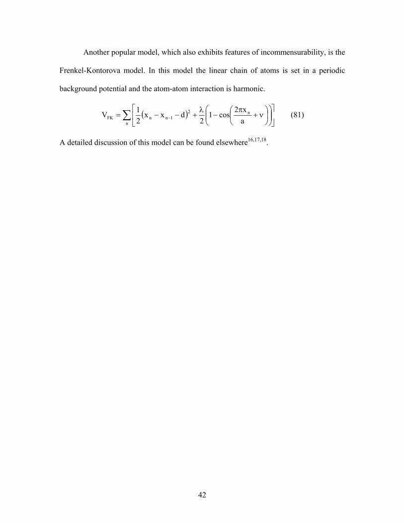
Another popular model, which also exhibits features of incommensurability, is the
Frenkel-Kontorova model. In this model the linear chain of atoms is set in a periodic
background potential and the atom-atom interaction is harmonic.
( )∑ ⎥⎦
⎤⎢⎣
⎡⎟⎟⎠
⎞⎜⎜⎝
⎛⎟⎠⎞
⎜⎝⎛ ν+
π−
λ+−−= −
n
n21nnFK a
x2cos1
2dxx
21V (81)
A detailed discussion of this model can be found elsewhere16, ,17 18.
42
4. Conjugated molecules.
In this Section we review the fundamental properties and applications of organic
conjugated molecules. Since the conjugated molecules which we investigated are used in
organic laser dyes and light-emitting devices, in the first subchapter particular emphasis
will be placed on the functioning of those devices and physical principles behind their
operation. In subsequent subsections we review some of the results of research on those
molecules.
4.1. Organic laser dyes and light-emitting devices (OLED).
4.1.1. Organic dyes.
Organic laser dyes, used as the active medium for tunable lasers, contain organic
molecules that absorb over a broad range of the spectrum and exhibit strong
luminescence19. A schematic diagram of energy levels of an organic dye molecule is
presented in Fig. 5. Electronic states with total spin equal to zero are called singlet states
and those with a total spin of one are called triplet states. S0-S2 are the singlet states and
T1 and T2 are triplet states. The electronic states have fine vibrational-rotational structure.
An excitation populates the S1 states and, after nonradiative relaxation to the bottom
level, the excited molecules spontaneously emit a photon and decay to a state in S0. Some
electrons, however, are excited to higher electronic states or decay to T1 states, from
43
which they can again be excited to T2 states. These absorption processes quench the laser
radiation.
Since the organic molecules absorb and emit over a wide range of wavelengths,
they are extremely useful for tunable lasers, in which the lasing wavelength can be
changed continuously. This is done by inserting a wave selective device, such as a grating
or prism, into the laser resonator. It is immediately evident that any change of the energy
levels can result in a dramatic change in the performance of these molecules as laser
dyes. Such changes can be caused by inducing transitions between possible molecular
conformations.
4.1.2. Organic light-emitting devices (OLEDs).
Another rapidly growing application of organic compounds is organic light-
emitting devices (OLEDs)20. In a light-emitting device, the active layer is sandwiched
between two electrodes, an anode that injects holes and a cathode that injects electrons.
An electron and a hole meet in the active layer, and an exciton is formed. This exciton
decays radiatively and light is emitted. This phenomenon is known as
electroluminescence, since an applied electric field is used to introduce charges into the
active layer. One of the electrodes (usually the anode) is made transparent to allow the
light to escape the device (Fig. 6). The wavelength of the emitted light is determined by
the energy difference between the highest occupied molecular orbital (HOMO) and the
lowest unoccupied molecular orbital (LUMO) of the active layer.
44

The first materials used in light-emitting devices were inorganic compounds such
as gallium arsenide. Recently, certain organic compounds have emerged as candidates for
optoelectronic applications. These molecules have delocalized π-orbitals which enable
them to transport charge. In order to serve as an active layer in an LED, the molecule
must also have significant overlap between its π-orbitals and those of neighboring
molecules. This overlap allows the charge to be transported in three dimensions. Suitable
compounds include poly(phenylene-vinylene) or PPV, tris(8-
hydroxyquinolinato)aluminium or Alq3, pentacene, and regioregular poly(3-
hexylthiophene)21. The difference between HOMO and LUMO energy levels in these
molecules is analogous to the band gap in conventional semiconductors.
In order to increase performance, the active layer is typically split into two layers.
One material is used as the hole transport layer and the other is used as the electron
transport layer. The electrodes are chosen to have a low work function for the anode and
a high work function for the cathode. The respective work functions should match the
electron affinity and ionization potential for active layers22.
The internal quantum efficiency of the LED is defined as the ratio of the number
of photons produced to the number of electrons flowing in the external circuit:
qrstint γ=η , (82)
where is the ratio of the number of exciton formation events to the number of electrons
flowing in the external circuit, is the fraction of excitons formed as singlets, and q is
the efficiency of radiative decay of those excitons. It is therefore necessary to achieve a
good balance between electron and hole currents, efficient capture of electrons and holes
in the emissive layer, and efficient radiative decay of singlet excitons.
γ
str
45

S0
S
S
1
2
1
2
Singlet states
Triplet states
Emiss
ion
Ener
gy
Figure 5. Schematic representation of the energy levels and electronic transitions
of an organic molecule used in laser dyes.
46
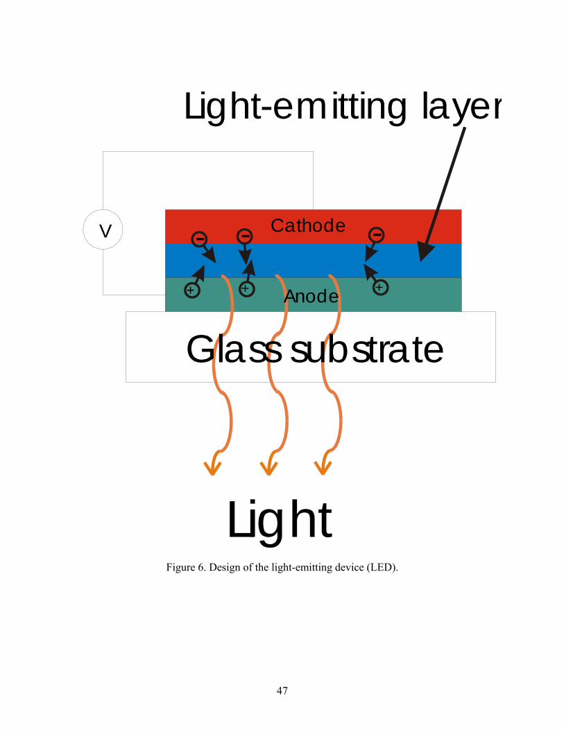
V Cathode
Light-emitting layer
- - -
Light
+ ++ Anode
Glass substrate
Figure 6. Design of the light-emitting device (LED).
47

One of the attractive features of OLED is that the color of emission can be
controlled by altering the chemical structure of the polymer film. Different side groups
can work to shift the emission both to the red and to the blue part of the visible spectrum.
The electrical characteristics of the single-layer devices are hard to model. The
typical current density-voltage characteristic resembles that of a diode. For PPV with Al
and indium-tin oxide (ITO) electrodes, for example, the majority of the current is
expected to be due to the holes. The formula relating current density J and voltage V is
given by:
⎥⎦
⎤⎢⎣
⎡−⎟
⎠⎞
⎜⎝⎛= 1
nkTqVexpJJ 0 , (83)
q is the carrier charge here. This formula, however, works best at voltages between 1 and
2 V and with n ranging from 1.8 to 2.4, compared to n=1 in the ideal case.
The OLEDs, especially multilayer devices, are quite complicated optical systems.
Their optical output is determined by many factors, including interference effects
between light taking different optical paths within the device. In the simplest model of
LED with isotropically oriented emitting dipoles the total amount of light produced,
is related to the light output per unit solid angle in the forward direction, , as follows:
totalF ,
0L
02
total Ln2F π= (84)
In the other limiting case, when all the dipoles are aligned within the plane of the film,
the emission is more preferably in the forward direction:
02
total LnF π= (85)
It should be mentioned that the presence of interfaces affect not only the angular
distribution of the light emitted, but also the radiative lifetime. For a more detailed
48

analysis the reader is referred to the references given in the review by Greenham and
Friend (Ref. 20).
The simplest model for organic diodes includes the charge transport equations
coupled with Poisson’s equation:
⎪⎪⎪
⎭
⎪⎪⎪
⎬
⎫
−επ
=∂∂
−=∂∂
+∂∂
−=∂∂
−∂∂
)np(e4xE
RGxJ
e1
tp
RGxJ
e1
tn
p
n
(86)
where the current densities are written in the form:
⎪⎪⎭
⎪⎪⎬
⎫
⎟⎠⎞
⎜⎝⎛
∂∂
−µ=
⎟⎠⎞
⎜⎝⎛
∂∂
+µ=
xp
ekTpEeJ
xn
ekTnEeJ
pp
nn
(87)
In these equations n(p) is the electron (hole) density, Jn (Jp) is the electron (hole) current
density, is the electron (hole) mobility, G (R) is the carrier generation
(recombination) rate, E is the electric field, e is the magnitude of the electron charge,
)( pn µµ
ε is
the static dielectric constant, and T is the temperature. The model is one-dimensional
because of the geometry of the device. The carrier mobilities are, in general, field
dependent. Their dependence is described by the Poole-Frenkel form23:
⎟⎟⎠
⎞⎜⎜⎝
⎛µ=µ
00 E
Eexp (88)
The electron-hole recombination is bimolecular, i.e. ( )npR γ= . For the recombination
coefficient, a Langevin form is often used:
49
εµπ
=γ me4
where is the larger of two mobilities. The generation rate is determined from the
detailed balance equation,
mµ
( )eepnG γ= , where ( )eepn is the product of equilibrium
electron and hole concentrations. For a more detailed discussion the reader is referred to
the Ref. 23 and references therein.
4.2. Conjugated molecules and their investigation.
4.2.1. Introduction.
As was mentioned in the previous section, molecules which have π-bonds in
addition to σ-bonds exhibit the ability to transport charge. Those molecules have
delocalized electrons due to the overlap of π-orbitals and are useful in applications such
as OLEDs24. Such molecules are called conjugated molecules. The overlap of π-orbitals
significantly affects their optical properties. If the overlap increases (for example, due to
application of pressure), the bandgap is red-shifted.
In their final form, the conjugated polymer molecules tend to be rigid molecules,
insoluble in common organic solvents. Therefore it is difficult to synthesize those
molecules directly, because the product will precipitate from the solution while its
molecular weight is still small. The final product is then difficult to form into the thin
film needed for the electronic devices. A number of methods have been developed to
overcome these problems. The most common one is a “precursor route” method, where a
50
soluble “precursor” polymer is prepared and processed to form a thin film. After this step,
further processing converts this film into the final polymer film.
The real polymers contain various defects, which break conjugation. These
defects highly affect the electronic properties of a conjugated polymer and, in turn, are
strongly dependent on the synthetic route and processing technique. The average number
of repeated units between conjugation-breaking defects is called the conjugation length.
Polyphenyls are one type of conjugated molecules. They consist of two or more
phenyl rings connected to each other via single C-C bonds. It was recognized long ago
(Ref. 27) that the rings in these molecules are free to rotate around the C-C bond. There
are several possible conformations that these molecules may have. One is the planar
conformation, where all the rings are in the same plane. Other conformations involve all
possible ring twists around the C-C bonds. For the simplest molecule of that type,
biphenyl, there is only one twisted conformation, with the planes of the rings being at
some nonzero angle with respect to each other. For p-terphenyl, p-quaterphenyl, and
other molecules with larger numbers of rings, there exist several possible twisted
conformations.
Now it is widely accepted that the conformation of any polyphenyl molecule is a
result of the balance between the electrostatic repulsion of hydrogen atoms, which tends
to twist the rings, and the interaction between π-electrons, which tends to planarize the
molecule25,26. In the solid state there is also an intermolecular packing force, which favors
the planar conformation. The outcome of the competition between these forces
determines the molecular structure.
51

The first experimental evidence that biphenyl molecules are twisted in the gas
phase was obtained in 194927. Since then, many investigations have been undertaken to
analyze not only biphenyl, but also higher-order polyphenyl molecules.
4.2.2. Biphenyl.
The biphenyl molecule (C12H10) consists of two phenyl rings connected by a
single C-C bond. In the gas phase, it is twisted, with the angle between ring planes
approximately 40°27. In the crystal phase, the molecule was determined to be planar28 at
room temperature. When the temperature is lowered, the structural transition to phase II
occurs at T=40 K, and the molecule becomes twisted29. Another phase transition, to phase
III, occurs at T=17 K. These phase transitions were studied by neutron diffraction30,
neutron scattering31, Brillouin scattering32, X-ray33, nuclear magnetic resonance (NMR)34,
electron paramagnetic resonance(EPR)35, and Raman scattering36. The schematic phase
diagram is shown in Fig. 7.
The two twisted phases of biphenyl are said to be incommensurate, which means
that the twist angle is modulated along the crystal structure. The change in the twist angle
can be expressed as follows31:
( ) ( ) ( )2s21s1 21cosAcosA Φ+⋅+Φ+⋅=φ rqrqr (89)
where and are modulation vectors, A1sq
2sq 1 and A2 are amplitudes, and Φ1 and Φ2 are
phases. The modulation vectors are related to the reciprocal lattice vectors ( , , )
by:
*a *b *c
52
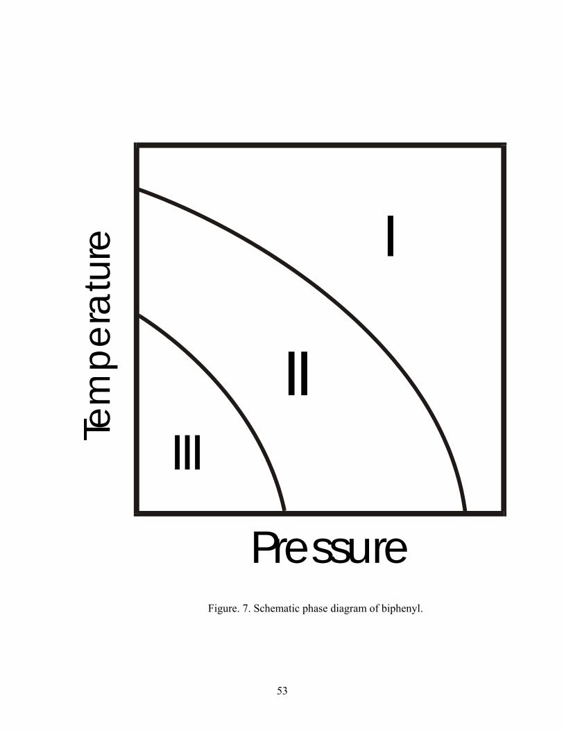
I
IIIII
Pressure
Tem
pera
ture
Figure. 7. Schematic phase diagram of biphenyl.
53

⎪⎪⎭
⎪⎪⎬
⎫
δ+δ−
+δ−=
δ−δ−
+δ=
***
***
cbaq
cbaq
cb
as
cb
as
212
1
2
1
(90)
for phase II. In phase III, 0ca =δ=δ so that the two modulation vectors coincide with
each other32,37.
Biphenyl has been studied very extensively over the past twenty-five years. The
phase transition is governed by a double-well potential, which is a result of the balance
between different forces, which was described earlier (Fig. 8). At low pressure the
intramolecular potential is stronger and the total potential has two minima. When
pressure increases, the crystal packing force prevails and the two minima merge to give
rise to a parabolic type of potential. The phase transition is of displacive type and is
characterized by a soft mode (see, for example, Ref. 38). A number of models have been
developed to describe the phase transition and incommensurability of the twisted phases
of biphenyl. In Ref. 39 the phase transition was induced by the coupling between the soft
torsional mode and acoustic phonon. A similar model was developed in Ref. 40, but the
effect of pressure was also included. In both cases the intra-molecular potential was
represented as:
42raint 4
B2AV ϕ+ϕ−= , (91)
where A and B are constants and ϕ is the twist angle of one ring (the total twist is 2ϕ).
The intermolecular potential tends to planarize molecules and can be written as:
∑∑≠
ϕϕ+ϕ=ji
jiiji
2ierint KLV , (92)
where i and j indicate lattice sites. The total potential is given by:
54
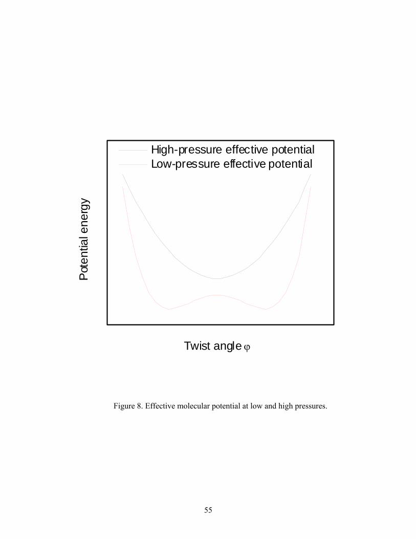
Pote
ntia
l ene
rgy
Twist angle ϕ
High-pressure effective potential Low-pressure effective potential
Figure 8. Effective molecular potential at low and high pressures.
55
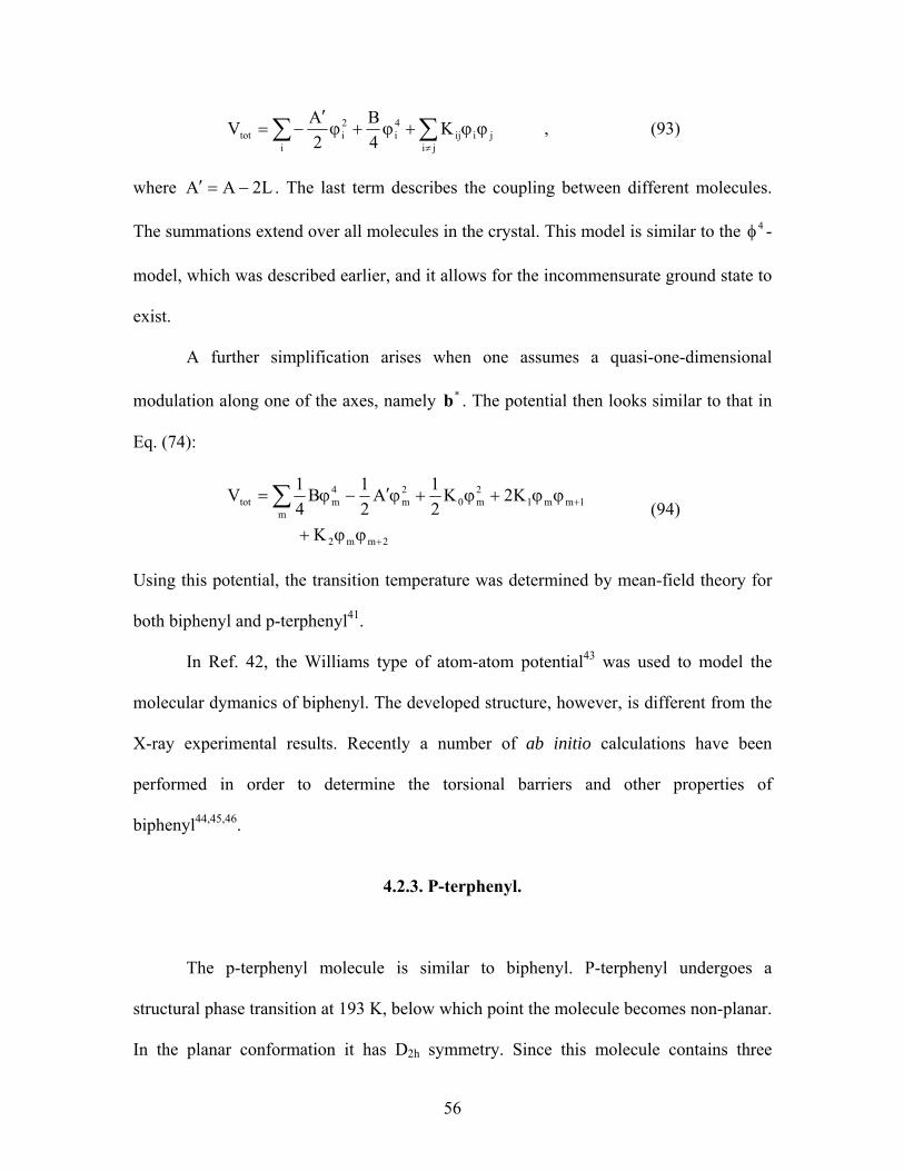
∑∑≠
ϕϕ+ϕ+ϕ′
−=ji
jiiji
4i
2itot K
4B
2AV , (93)
where . The last term describes the coupling between different molecules.
The summations extend over all molecules in the crystal. This model is similar to the -
model, which was described earlier, and it allows for the incommensurate ground state to
exist.
L2AA −=′
4φ
A further simplification arises when one assumes a quasi-one-dimensional
modulation along one of the axes, namely . The potential then looks similar to that in
Eq. (74):
*b
2mm2
m1mm1
2m0
2m
4mtot
K
K2K21A
21B
41V
+
+
ϕϕ+
ϕϕ+ϕ+ϕ′−ϕ= ∑ (94)
Using this potential, the transition temperature was determined by mean-field theory for
both biphenyl and p-terphenyl41.
In Ref. 42, the Williams type of atom-atom potential43 was used to model the
molecular dymanics of biphenyl. The developed structure, however, is different from the
X-ray experimental results. Recently a number of ab initio calculations have been
performed in order to determine the torsional barriers and other properties of
biphenyl44, ,45 46.
4.2.3. P-terphenyl.
The p-terphenyl molecule is similar to biphenyl. P-terphenyl undergoes a
structural phase transition at 193 K, below which point the molecule becomes non-planar.
In the planar conformation it has D2h symmetry. Since this molecule contains three
56

phenyl rings, there are several possible models for the non-planar structure. In Ref. 47, it
was shown by x-ray diffraction that the central ring becomes twisted, with twist angles of
16 and 25° with respect to external ones. This molecule possesses C2h symmetry. As with
biphenyl, p-terphenyl has an incommensurate phase, such that twist angle is modulated
throughout the crystal. Unlike biphenyl, however, the p-terphenyl molecule preserves its
center of symmetry upon the phase transition. The rotational disorder in the
incommensurate phase was explained by considering non-bonded interactions48, using the
Williams-type of potential49. The temperature-induced phase transition was studied by
fluorescence emission50, Raman scattering51, ,52 53, Brillouin scattering54, NMR55, EPR56,
and by infrared (IR) spectroscopy57. It was shown in Refs. 52 and 57 that certain Raman
and IR peaks disappear upon the phase transition, when the temperature is raised above
the critical point.
A number of theoretical investigations have been carried out to determine the
structure of the p-terphenyl molecule. In Ref. 58 semi-empirical calculations, using the
INDO-type method59, have shown that the p-terphenyl molecule has two nearly
isoenergetic isomers of D2 and C2h symmetries, with D2 being slightly more stable than
C2h. Akiyama60 has determined, using similar methods, that p-terphenyl in solution has
C2 symmetry. In Ref. 64, p-terphenyl was studied in a carbon disulfide solution, and the
analysis of infrared band intensities led the authors to conclude that the conformation in
solution has D2 symmetry. This conclusion contradicted the theoretical results of
Akiyama (Ref. 60). A conformational analysis of various isomers of p-terphenyl by
photoelectron spectroscopy has also been performed61,62. It was found that p-terphenyl in
57

the gas phase has twisted conformation, with twist angle of about 42°, whereas in the
solid state at room temperature it is planar.
It is evident that hydrostatic pressure provides an excellent tool for studying phase
transitions, especially those which involve a balance between inter- and intramolecular
forces. Pressure shifts this balance by increasing the intermolecular forces. At low
temperatures and pressures, the polyphenyl molecule is in its twisted conformation. As
pressure increases, it goes through a phase transition and becomes planar. The influence
of pressure on the conformation of p-terphenyl has been studied by Raman scattering63,
infrared absorption64, and optical absorption65. The observed changes in the spectra
clearly indicated the presence of a phase transition.
4.2.4. P-quaterphenyl.
The p-quaterphenyl molecule resembles biphenyl and p-terphenyl in its behavior.
This compound is planar at room temperature and undergoes a phase transition at T=243
K, when the molecule becomes twisted. Similarly, the molecule planarizes when the
pressure is increased. Analogously to biphenyl, this molecule loses its center of inversion
symmetry upon the phase transition. The symmetry group in the low-pressure and low-
temperature phase is D2. Quaterphenyl was also investigated by different techniques
mentioned earlier for biphenyl and p-terphenyl, but not as extensively96,52,66.
58

5. Experimental methods.
In this Section we review devices used in high-pressure research and Fourier-
transform infrared spectroscopy, methods of achieving high pressure, pressure
monitoring, infrared spectroscopy techniques, and advantages of Fourier-transform
spectroscopy compared to other spectroscopic methods.
5.1. High-pressure apparatus.
5.1.1. Diamond-anvil cells.
The experimental task to achieve very high pressures has been a major challenge
for scientists. The invention of the diamond anvil cell (DAC) provided an extremely
powerful tool for reaching pressures in the megabar region (1 megabar=106 atm=103
kbar=100 GPa). The first DAC is attributed to the work of Lawson and Tang67, who used
a diamond to achieve high pressures for x-ray diffraction studies. A decade later, two
other versions of DACs appeared independently68,69 and the DAC has been widely used
in high-pressure physics ever since.
Here I present a review of DACs and their applications to high-pressure research,
following the review given by Jayaraman70.
There are several types of DACs, among which five major types are
distinguished. They are the National Bureau of Standards cell, Bassett cell, Mao-Bell cell,
Syassen-Holzapfer cell, and Merrill Bassett cell. These cells are shown in Fig. 9-13 [70].
59
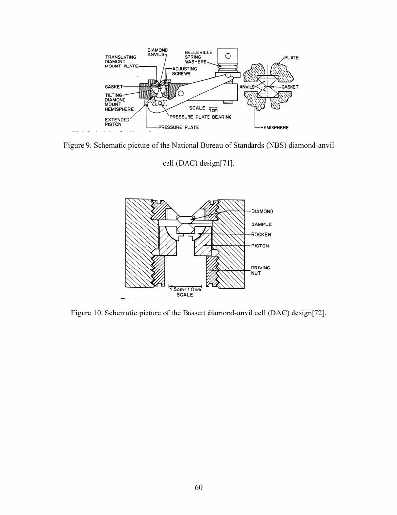
Figure 9. Schematic picture of the National Bureau of Standards (NBS) diamond-anvil
cell (DAC) design[71].
Figure 10. Schematic picture of the Bassett diamond-anvil cell (DAC) design[72].
60

Figure 11. Schematic picture of the Mao-Bell diamond-anvil cell (DAC) design [73].
Figure 12. Schematic picture of the Syassen-Holzapfer diamond-anvil cell (DAC) design
[74].
61

Figure 13. Schematic picture of the Merill-Bassett diamond-anvil cell (DAC) design [75].
62
All these cells use diamonds as anvils. The sample is placed between two flat
surfaces of the diamonds and the force is applied to push the diamonds together. Since
the areas of the diamond surfaces are small, a DAC is usually capable of achieving a
pressure of hundreds of kbar. The Mao-Bell cell is superior to the other types of cells,
being able to reach pressures up to several megabar. The diamonds have a typical size of
1/8 to ½ carat with an anvil flat (culet) diameter ranging from 0.3 to 0.7 mm. The
diamonds are shaped in the forms of octagons or polygons with as many as 16 sides. The
surface opposite to the culet is of 2 to 5 mm in diameter. Generally, larger diamonds are
preferred for larger pressures.
The metal gasket for the DAC was first introduced in 1965 (Ref. 76). The gasket
is preindented by the culets to a thickness of 0.05 to 0.2 mm. A hole is then drilled in the
center of the indentation and the sample of interest is put in the hole, together with a ruby
chip for pressure calibration. A pressure-transmitting fluid is also placed in the hole to
provide hydrostatic pressure. In addition to confining the sample, the gasket provides
support to the diamonds. Beveling of the edges of the anvils is required for megabar
pressures.
Pressure calibration in the DAC is made via the ruby fluorescence method77,78.
This calibration technique uses the ruby fluorescence lines, which at atmospheric
pressure are at 692.7 and 694.2 nm. These lines shift linearly with pressure up to 200
kbar79. For higher pressures, a correction is required due to the nonlinearity of the shifts.
The following formula has been proposed for the pressure determination80:
( )[ ]113808P 5 −+λλ∆= , (95)
63

where P is in kbar and λλ∆ is the fractional shift in wavelength. Ruby fluorescence has
been the preferred pressure calibration method for the past twenty five years.
Many fluids are suitable for providing hydrostatic pressure. The range of
pressures at which the liquid has hydrostatic behavior varies from 90 kbar for argon to
more than 600 kbar for helium and hydrogen. In Table II, data for several pressure-
transmitting liquids are summarized.
Diamond-anvil cells have long been used for spectroscopy. The transparency of
diamond, over a wide spectral range, makes it a very useful material for high-pressure
spectroscopy. However, the culet size of the diamonds is small, and the gasketing reduces
the working space even further. As a result, one has to deal with tiny apertures of about
0.3 mm in diameter. This drastically reduces the signal from the detector. In general, the
researcher has to focus the light onto the sample and bring the detector as close to the
sample as possible.
In the present experiments, a piston-cylinder DAC was used. The alignment
system consists of three screws to adjust the orientation for the diamond mounted on the
hemispherical backing plate. Three other screws are used to adjust the translational
alignment of the other diamond. The pressure is provided by tightening six Allen screws
placed at the corners of a regular hexagon, as viewed along the axis of the cell. The
piston has a polished cone that helps to focus the light onto the sample. The detector is
located at the opposite side of the top diamond. The whole assembly is attached to the
sample holder and the parabolical mirror is used to focus the light onto the sample (Fig.
14).
64

IR beam
Detector
Backing platesGasket
PistonCylinder
Mirror
Diamonds
Allen screwsSample
Figure 14. Schematic representation of the low-temperature high-pressure IR-
spectroscopy device.
Table II. Some pressure media and their pressure ranges (Ref. 70).
Medium Freezing pressure at RT (kbar)
Pressure range of hydrostatic
behavior (kbar) Comments
Methanol:ethanol 4:1 104 ~200 Easy filling
Methanol:ethanol: Water 16:3:1 145 ~200 ″
He 118 >600 Cryogenic or high-pressure filling
Ne 47 160 ″
Ar 12 90 ″
Xe -- 300 Cooling below 165 K needed
H2 57 >600 Cryogenic or high-pressure filling
D2 253 ± -- ″
N2 24 130 Cryogenic filling
O2 59 -- ″
65
The sample holder is placed into the cryostat, where the low-temperature
measurements are performed. The DAC can also be used for room temperature
measurements.
5.1.2. Diamond-anvil cell alignment.
After the diamonds are placed on their base plates, they must be aligned in order
to provide high pressure without cracking. The first condition for alignment is
parallelism, in which the culet surfaces are parallel to each other. This is accomplished by
adjusting screws for the hemispherical base plate. During these fine adjustments,
interference fringes are observed in the microscope. The goal is to make the fringes as
broad as possible, in which case the culet surfaces are almost parallel to each other. After
this task was completed, translational alignment is performed. Again, looking into the
microscope allows one to monitor the two culet surfaces. After the diamonds are aligned,
the Allen screws are tightened slightly to make the fringes completely disappear. This
procedure ensures nearly perfect parallelism of the culet planes. Three reference points
are marked on the piston and their heights are measured with an indicator, to an accuracy
of 2 µm. The relative heights of these points must be maintained throughout the
experiment.
66
5.1.3. Diamond-anvil cell loading.
We used a circular piston-cylinder type DAC, similar to the cell described in Ref.
81, with type I diamonds with culet diameters of 700 µm. A stainless steel gasket of 250
µm thickness was pre-indented to 100 µm. A hole of 340 µm in diameter was drilled in
the center of the indentation, using a carbide drill. A sample was placed in the hole and
the whole cell was assembled and immersed in liquid nitrogen. Compressed helium gas
was bubbled into the liquid nitrogen to suppress boiling. Liquid nitrogen seeped into the
hole in the gasket. Then the Allen screws were tightened to apply force to the diamonds
and pressure to the nitrogen and the sample. The cell was then taken out of the liquid
nitrogen and warmed up to room temperature. The condition of the sample was checked
with the microscope. The relative height of three reference points, mentioned in the
previous section, was measured and adjustments are made, if necessary, to maintain
alignment. Subsequent pressure adjustments were made by either loosening or tightening
one or more of the Allen screws.
5.1.4. Low-temperature measurements.
After the loading was completed, the cell was mounted onto the sample holder
and put into a Janis continuous-flow liquid-helium cryostat with wedged zinc selenide
windows. The temperature was maintained at approximately 8 K. The pressure was
determined by measuring the vibrational frequency of CO2 in the nitrogen matrix. Its
67
pressure dependence was determined in Ref. 82. Thus it serves as good in situ pressure
calibration in the range from 0 to 7 GPa.
5.1.5. Fluorescence measurement system.
As was mentioned before, one of the most common methods to determine the
pressure in a DAC is to measure the shift of the ruby fluorescence lines. Our fluorescence
measurement system consists of a monochromator, a charge-coupled device (CCD) array
detector, a controller, and a computer. Green laser light (532 nm) from a laser pointer is
the excitation source for the ruby fluorescence. The detection system uses a liquid
nitrogen (LN) cooled CCD detector and Acton SpectraPro 300i
monochromator/spectrograph. It has three gratings, which cover a broad range of the
spectrum from visible to near-infrared. In order to suppress the signal from the laser light,
a red filter is placed in front of the spectrograph slit. The controller is programmed by the
computer and determines the setup for spectra acquisition. The detector must be cooled to
LN temperature. In order to maintain the appropriate temperature, a 1.7 liter Dewar is
mounted on the back side of the CCD matrix. When filled with liquid nitrogen, the
Dewar maintains the necessary temperature for approximately 30 hours. The
commercially available software WinSpec32 is installed onto the computer and is used to
save and analyze all the data obtained.
68

5.2. Fourier transform infrared spectroscopy (FT-IR).
5.2.1. Basic theory of FT-IR.
Fourier-transform infrared spectroscopy (FT-IR) is an important technique used in
biology, chemistry, and physics. The discussion in this section follows the review given
by Griffiths83. The basis for FT-IR spectroscopy is the Michelson interferometer (Fig.
15). A broadband beam of radiation from the source impinges on the beam splitter, where
it is partially reflected to the fixed mirror and partially transmitted to the movable mirror.
The two beams are reflected back to the source and onto the detector. When the two
mirrors are at the same distance from the beam splitter, the path difference between the
two beams is zero and they interfere constructively.
When one of the mirrors is moved, a path difference δ is introduced, and there is
a nonzero phase shift between the two beams. The intensity of the beam at the detector is
given by the following expression:
( ) ( ) ( )[ ] ( ) ( )[ ]δπ+=λδπ+λ=δ k2cos1kI5.02cos1I5.0I , (96)
where is the wavelength and k is the wave number, λλ
=1k . The cosinusoidal part of
Eq. (96) is the interferogram, and will be of interest in this discussion. The spectrometer
obtains the value . The real intensity as a function of wave number, I(k), is obtained
via Fourier transformation of
( )δI
( )δI . This transformation is given by:
( ) ( ) ( )∫+∞
∞−
δ⋅δπδ= dk2cosIkI . (97)
69
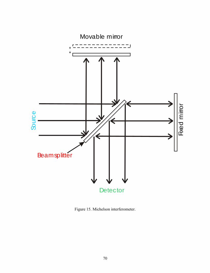
Movable mirror
Fixed
mirr
or
Sour
ce
Detector
Beamsplitter
Figure 15. Michelson interferometer.
70

For real systems, we must introduce two corrections. The first takes into account the
efficiency of beamsplitter, amplification characteristics, and detector response.
Experimentally, we obtain not the true I(k), but some other function B(k), due to these
factors. The second correction accounts for the fact that the path length difference is
limited by a maximum value . Thus the spectrum obtained will be given by: ∆
( ) ( ) ( ) ( )∫+∞
∞−
δ⋅δπδδ= dk2cosDIkG , (98)
where is the truncation function, which is zero for all ( )δD ∆>δ . The shape of this
function can be quite arbitrary, the simplest being the boxcar function, which is equal to
one for all ∆<δ .
The function G(k) can be viewed as the convolution of the true spectrum, B(k),
and the Fourier-transform of the truncation function, ( )δD :
( ) ( ) ( )∫+∞
∞−
′⋅′−′= kdkkfkBkG , (99)
where f(k) is given by:
( ) ( ) ( )∫∆
∆−
δ⋅δπδ= dk2cosDkf . (100)
The function f(k) is called the instrument line shape (ILS). For the boxcar truncation
function and monochromatic spectral line of wavenumber , we obtain for G(k): 1k
( ) ( ) ( )[ ]( )∆−π
∆−π⋅⋅∆=
kk2kk2sinkB2kG
1
11 . (101)
It turns out that the spectral resolution can be affected by the choice of the
function . There are many types of truncation functions, and for some of them the ( )δD
71
side oscillations in the interferogram are suppressed. This suppression is called
apodization and the appropriate ( )δD is called the apodization function. A more detailed
discussion of this problem can be found elsewhere84.
Other factors affecting the performance of Fourier transform spectrometers are the
beam divergence, mirror misalignment, and poor mirror drive. The first factor sets the
limit for the achievable resolution, k∆ , to be
2maxkk α=∆ , (102)
where is the divergence angle and kα max is the maximum wave number in the spectrum.
A detailed derivation of Eq. (102) can be found in Ref. 83.
For an ideal spectrometer, the ratio of the intensity at zero path difference to the
intensity at large path difference is two. Therefore, the parameter R,
( ) ( )( )∞
∞−=
II0IR (103)
is equal to 1. For a real spectrometer, the value of R gives a measure of how well the
interferometer is aligned.
A poor mirror drive can lead to a loss in resolution. If the mirror is tilted by an
angle β , then the difference in retardation, δ∆ , is:
β≈β=δ∆ D2tanD2 (104)
for small , where D is the beam diameter. A loss in resolution occurs when β λ>δ∆ 1.0 .
Then the tilt angle must satisfy the following inequality:
maxDk201
≤β . (105)
72

For D=5 cm and kmax=5000 cm-1 the angle β must be less than 2 µrad. The critical angle
may be increased by aperturing the beam, but only at the cost of a decrease in beam
intensity.
To obtain a spectrum, an inverse Fourier transform must be performed [Eq.(97)].
Cooley and Tukey85 developed a fast Fourier transform (FFT) algorithm, which uses a
low number of operations. Another important issue is the phase correction, due to optical,
electronic, and sampling effects. There are several methods to address the problem of
phase correction, most famous of them being described by Mertz86 and Forman87.
5.2.2. Beer’s Law.
While traveling through an absorbing medium, a beam of radiation decreases in
intensity. The change in intensity is proportional to intensity itself:
IndxdI
σ−= , (106)
where is the absorption cross section and n is the concentration of absorbing particles.
Assuming that the concentration is uniform in space, we obtain Beer’s law:
σ
dn0eII σ−= , (107)
where d is the thickness of the sample. The beam intensity exponentially decreases with
the thickness of the medium through which the beam travels.
Beer’s law is valid for dilute solutions. Deviations may arise due to a non-uniform
distribution of absorbing centers, stray light coming into the system, or nonlinear effects
at high intensities. In general, the absorption cross section is frequency dependent. For
example, a system absorbs light at the vibrational frequencies of the molecules
73

composing it. This absorption is seen in the spectrum as “dips” in the intensity measured
by the detector.
5.2.3. Beamsplitters for FT-IR spectrometers.
One of the most important parts of the FT-IR spectrometer is the beamsplitter.
Suppose that a beamsplitter has a reflectance R and a transmittance T. Neglecting any
absorption of radiation in the beamsplitter, we can write:
1TR =+ (108)
It can be shown that if the incident intensity is I, then the intensity of light going towards
the detector is given by ( . Given Eq. (108), the value of 2RT reaches maximum at
R=T=0.5, at which point it 2RT=0.5. This explains the appearance of the coefficient 0.5
in Eq. (96), where we implicitly assumed an ideal beamsplitter. To account for an
imperfect beamsplitter, Eq. (96) can be rewritten as:
)IRT2
( ) ( ) ( ) ( )[ ]δπ+η=δ k2cos1kIk5.0I , (109)
where . The function ( ) RT4k =η ( )kη is known as the relative beamsplitter efficiency
and should be as close to unity as possible over the widest possible spectral range. Some
materials that are used as beamsplitters include polyethylene terephthalate (Mylar),
germanium, CsI, CsBr, and KBr. The two most commonly used materials are Mylar and
KBr. The choice of beamsplitter is dictated by the spectral range of interest. Mylar is
used in the far-infrared region, whereas in the mid-infrared region it is necessary to use
KBr.
74

5.2.4. Infrared detectors.
Infrared detectors are usually divided into two major classes: thermal detectors
and quantum detectors. Thermal detectors sense the change in the temperature of the
absorbing material. Such a change can result in electromotive force (thermocouple),
change in resistance (bolometer, thermistor), movement of a membrane caused by
thermal expansion of a gas (pneumatic detector), which, in turn, causes the change in
illumination of auxiliary cell (Golay detector). Thermal detectors are usually slow. The
most sensitive are Golay detectors and pyroelectric bolometers. Thermal detectors are
usually used in the far-infrared spectral region.
Quantum detectors use the property that photons can excite electrons in solids
from the valence band into the conduction band. Some of these detectors use impurity
atoms, which absorb photons with energies lower than the band gap. Examples include
PbS, mercury cadmium telluride (MCT), germanium doped with copper, gallium or
antimony, and InSb. Quantum detectors are much faster than thermal detectors. However,
these detectors have a sharp cutoff at low wavenumbers, and their response is influenced
by thermal noise. This leads to the requirement that these detectors need to be cooled.
Some detectors, like MCT, operate at liquid nitrogen temperature (77 K). Others, like
doped germanium, require liquid helium temperatures (4.2-12 K). Quantum detectors are
used in the mid- to near-infrared spectral range.
75
5.3. Advantages of FT-IR spectrometers.
Besides the FT-IR spectrometers there are also various grating IR spectrometers.
Their relative performance is very important to know when choosing among them for the
particular experiment. There exist theoretical criteria to judge the relative efficiency of
two spectrometers, which will be discussed below. Also practical results have been
obtained and will be described as well.
5.3.1. Jacquinot’s advantage.
An important parameter which characterizes the efficiency of a spectrometer is
the throughput. The throughput is defined as the product of the beam area and its solid
angle at any focus. For the Fourier spectrometer, the throughput is given by:
Fmax
F Ak
k2 ∆π=Θ , (110)
where AF is the area of the mirrors that are illuminated. For the grating spectrometer the
throughput is:
2G
G kafkhA ∆
=Θ , (111)
where h is the height of the slit, f is the focal length of the collimating mirror, a is the
grating constant. The ratio of two throughputs, J, known as Jacquinot’s advantage, is
given by:
76
maxG
2F
hkAkafA2J π
= . (112)
A calculation of J for several spectrometers showed that for all but very low
wavenumbers, the FT-IR spectrometer is significantly better than a grating spectrometer
(see, for example, Ref. [88]).
5.3.2. Fellgett’s advantage.
The signal-to-noise ratio (SNR) for a Fourier spectrometer will be greater than the
SNR for a grating spectrometer by a factor of M , where M is the number of resolution
elements, provided that all other parameters are the same. For example, for the mid-
infrared spectrum taken in the range from 400 to 4000 cm-1 with a resolution of 1 cm-1,
Fellgett’s advantage will be 603600 = . In addition, the time advantage for an FTIR
spectrometer is directly proportional to M.
Combining Jacquinot’s and Fellgett’s advantages, it can be shown that a Fourier
spectrometer will be 2000-3000 times more sensitive than a grating spectrometer. In
practice, however, a smaller advantage is observed. This is due to noise arising from
other parts of the FTIR spectrometer, mainly the detector.
5.3.3. Fourier-transform infrared (FT-IR) spectrometry.
The DA8 Bomem FT-IR spectrometer was used in obtaining the data for this
work. A Globar, which is a heated ceramic, was used as a broadband light source (200 to
77

10000 cm-1). The beamsplitters used were KBr for the mid-infrared region (450 to 5000
cm-1) and Mylar for far-infrared region (125 to 850 cm-1). The pressure inside the FT-IR
compartment is maintained at a level of 2.0≤ Torr and the Globar is cooled by the flow
of chilled water. The moving mirror velocity can vary from 0.01 to 4 cm/s and the
aperture ranges from 0.5 to 10 mm. Mirrors alignment is maintained with the help of a
He-Ne laser. Monochromatic laser light creates an interferogram and several detectors
sense it. If the mirrors are out of alignment, the interferograms for different detectors
exhibit relative phase shift, which can be measured. This shift gives the signal for
alignment transducers to correct the misalignment.
For room-temperature measurements, we used an MCT detector for mid-infrared
spectra and a DTGS detector for the far-infrared. For low-temperature measurements, a
Ge:Cu photoconductive detector was used. Its operation is limited to liquid helium
temperatures. The spectrometer is connected via Ethernet cable to the computer with
PCDA software for the data acquisition and the GRAMS software package to process and
analyze the spectra.
78

6. Present work.
6.1. Organic conjugated molecules under pressure.
Although the investigation of polyphenyls has been quite extensive, there are
relatively few reports on high-pressure research on these molecular solids. The
conformation of p-terphenyl in its twisted conformation is still under question. In the
following sections, the results of FTIR spectroscopy on biphenyl, p-terphenyl, and p-
quaterphenyl under hydrostatic pressure are presented.
6.1.1. Biphenyl.
6.1.1.1. Experimental results.
In this section, high-pressure IR spectroscopy experiments on biphenyl are
discussed. Some of these results have been published in Ref. 89.
Two samples were investigated. First, protreated biphenyl ( ), hereafter
referred to simply as biphenyl, was measured. Second, deuterated biphenyl ( , or
biphenyl-d
1012HC
1012DC )
10, was measured. In the latter sample, every hydrogen was replaced by a
deuterium, with an isotopic purity of 98%90. The IR spectra for biphenyl are shown in
Fig. 16 and spectra for deuterated biphenyl are shown in Fig. 17. Resolution was 2 cm-1.
79

500 550 600 650 700 750 800
(a)
P=0.97 GPa
P=0.05 GPa
Tran
smis
sion
(a.u
.)
Wave number (cm-1)
880 900 920 940 960 980 1000
(b)
P=0.97 GPa
P=0.05 GPa
Tran
smis
sion
(a.u
.)
Wave number (cm-1)
Figure 16. Biphenyl spectra at pressures below and above phase transition.
IR-modes, that disappear upon transition, are indicated by arrows.
80
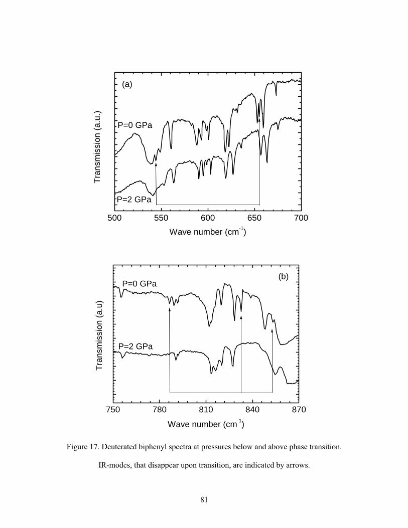
500 550 600 650 700
(a)
P=0 GPa
P=2 GPa
Tran
smis
sion
(a.u
.)
Wave number (cm-1)
750 780 810 840 870
(b)P=0 GPa
P=2 GPa
Tran
smis
sion
(a.u
)
Wave number (cm-1)
Figure 17. Deuterated biphenyl spectra at pressures below and above phase transition.
IR-modes, that disappear upon transition, are indicated by arrows.
81

By progressively increasing the pressure we found that certain peaks disappear
when the pressure rises above certain value. Those peaks that disappear are indicated by
arrows. The spectral range from 500 to 1100 cm-1 corresponds to out-of-plane motion of
hydrogen atoms in which the atomic displacement is perpendicular to the plane of the
appropriate ring. There are three peaks in the biphenyl spectrum in the range 500-800
that disappear upon the phase transition [Fig. 16(a)]. The spectral range from 1100
to 1800 cm
1cm−
-1 includes in-plane hydrogen bending modes. Upon substitution with
deuterium, hydrogen-related frequencies should decrease by some factor, which in an
“ideal” case is 2 . From Fig. 17(a) it is seen that there are two peaks, at 545 and 655 cm-
1, that disappear in deuterated biphenyl. Relative to the hydrogen peaks at 679 and 790
cm-1 [Fig. 16(a)], the deuterium peaks are shifted downward by a factor less than 2 . The
deviation from the ideal case is due to anharmonic effects as well as significant motion of
the carbon atoms (see Appendix B). In the observed spectra the strongest peaks were
found to be due to out-of-plane hydrogen motion.
The pressure-dependent shifts of several out-of-plane hydrogen bending modes
are plotted for biphenyl in Fig. 18. In Fig. 19 we plotted the normalized intensities for
two peaks that disappear after the phase transition, as a function of pressure.
Uncertainties in data are smaller than the size of points in Fig. 18, 19. The intensity of the
peak at approximately 836 cm-1 was chosen as a reference for the normalization. At a
pressure between 0.07 and 0.4 GPa, the integrated absorbance of the peaks at 790 and
841 cm-1 drops to zero, to within experimental uncertainty. Our results are in agreement
with those of Ref. 36, which reported a phase transition at 0.18 GPa.
82

0.0 0.2 0.4 0.6 0.8 1.0 1.2 1.4 1.6770
780
790
830
840
850
Wav
e nu
mbe
r (cm
-1)
Pressure (GPa)
Figure 18. Frequency dependence of several IR-modes on the pressure for biphenyl.
0.0 0.2 0.4 0.6 0.8 1.0 1.2 1.4 1.6
0.0
0.2
0.4
0.6
0.8
1.0
ν=789.7 cm-1
ν=840.7 cm-1
Nor
mal
ized
inte
nsity
Pressure (GPa)
Figure 19. Normalized intensity dependence on the pressure for two IR-modes that
become IR-inactive upon phase transition for the biphenyl molecule.
83

6.1.1.2. Group theory.
To explain the disappearance of IR activity for certain vibrational modes, we
applied group theory to analyze the normal vibrational modes of the molecules. The z-
axis in our analysis is directed along the main axis of the molecule, the x-axis is in the
molecular plane for the planar conformation, and the y-axis is perpendicular to the plane.
A schematic diagram of biphenyl in its twisted conformation is shown in Fig. 20.
The twisted conformation of biphenyl belongs to the D2 point group. The
vibrational modes can be classified as follows:
Γ = 15A ⊕ 13B1 ⊕ 16B2 ⊕16B3
Modes belonging to the B1, B2, or B3 irreducible representations are IR-active, for a total
of 45 IR-active modes. For the planar configuration, biphenyl belongs to the D2h point
group. The vibrational modes are given by:
Γ = 11Ag ⊕ 4Au ⊕ 3B1g ⊕ 10B2g ⊕ 6B3g ⊕ 10B1u ⊕ 6B2u ⊕10B3u
Modes belonging to the B1u, B2u, or B3u irreducible representations are IR-active, for a
total of 26 IR-active modes. Upon planarization, some of the B1, B2, and B3 modes
transform into B1g, B2g, and B3g modes, which are IR-inactive. This disappearance of
certain IR absorption peaks is in qualitative agreement with our experimental
observations.
84
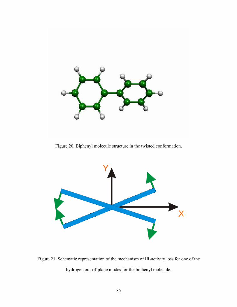
Figure 20. Biphenyl molecule structure in the twisted conformation.
Y
X
Figure 21. Schematic representation of the mechanism of IR-activity loss for one of the
hydrogen out-of-plane modes for the biphenyl molecule.
85

In Fig. 21, one of the B3 modes is shown schematically. The cross sections of the
phenyl rings are represented as rectangles and the dipole moments, induced by the motion
of hydrogen atoms, are shown by the arrows. In the twisted conformation, the mode has a
net induced dipole moment in the x-direction. In the planar conformation, the dipoles
exactly cancel, so that the mode is IR-inactive.
6.1.1.3. Numerical calculations.
Ab initio and DFT calculations are used extensively to model molecular and
atomic systems. The biphenyl structure has been numerically calculated by previous
researches91,92. In this work, calculations have been performed in order to simulate the IR
spectra of biphenyl and deuterated biphenyl, using Gaussian 98W (Ref. 9). We used the
density functional theory (DFT) Becke 3-parameter method93 with the Lee-Yang-Parr
correlation functional and the basis set 6-31G(d). The details about calculations and basis
sets have been described previously.
For the twisted structure, the calculated dihedral angle between two phenyl rings
is 38º for biphenyl and 35º for deuterated biphenyl. Electron diffraction experiments on
biphenyl in the gas phase yielded a dihedral angle of 40º (Ref. 27), in good agreement
with our calculations. Numerical optimization of the geometric structure of the molecules
yields a configuration that belongs to the C2 point group. This low symmetry is due to a
distortion of the phenyl rings. However, the deviation from planarity in each phenyl ring
is very small. To a good approximation, we can consider this molecule as belonging to
the D2 point group, and our previous group-theory analysis remains valid.
86

Table III. Vibrational modes in biphenyl ( ) that are IR active in the twisted
conformation but IR inactive in the planar conformation.
1012HC
Calculated Experimental
Frequency
(cm-1)
Normalized
intensity
Symmetry Mode character Frequency
(cm-1)
Normalized
intensity
559.9 0.2622 B3 H out-of-plane 552.9 0.272
628.6 0.0006 B2 C-H in-plane NDa NDa
714.7 1 B3 H out-of-plane 679.3 0.745
796.9 0.88 B3 " 789.7 1
860.9 0.086 B1 " 840.7 0.720
938.5 0.15 B3 " 912.1 0.041
968.7 0.1248 B2 " 965.8 0.377
995.6 0.0096 B2 " NDa NDa
1116.1 0.061 B1 H in-plane NDa,b NDa,b
1192.9 0.0002 B3 " NDa,b NDa,b
aND = not discovered.
bCalculated frequency lies within diamond absorption band.
87

Table IV. Vibrational modes in deuterated biphenyl ( ) that are IR active in the
twisted conformation but IR inactive in the planar conformation.
1012DC
Calculated Experimental
Frequency
(cm-1)
Normalized
intensity
Symmetry Mode character Frequency
(cm-1)
Normalized
intensity
567.07 1 B3 D out-of-plane 544.5 0.340
602.82 0.0018 B2 D in-plane+ring
distortion
NDa NDa
668.63 0.14 B3 D out-of-plane 655.3 0.752
670.04 0.1456 B1 " NDa NDa
784.29 0.264 B1 D out-of-plane+ring
distortion
786.3 0.337
789.11 0.161 B3 " 789.5 0.444
838.72 0.4535 B3
D in-plane+ring
distortion
832.5 1
844.02 0.0789 B2 D in-plane 838.8 0.187
862.8 0.0301 B2 " 853.0 0.188
1071.88 0.0005 B2 " NDa NDa
aND=not discovered
88
The vibrational spectra calculations were made with the symmetry restricted to
the D2 point group. The planar conformation of the molecule, belonging to the point
group, turns out to be stable during the calculations. One of the calculated frequencies is
imaginary, however, indicating that the planar configuration is not a minimum on the
potential energy surface.
h2D
A correspondence was made between vibrational modes in the planar and twisted
conformations by examining similarities in the character of motion, reduced mass,
frequency, and IR intensity for any given pair of modes. Frequencies that are IR-active in
the twisted conformation but IR-inactive in the planar conformation, as predicted by this
computation for the twisted conformation of biphenyl, are listed in Table II together with
the experimental results. The frequencies for vibrational modes in deuterated biphenyl are
given in Table III. In biphenyl, we did not observe hydrogen in-plane modes because the
frequencies of those modes lie within the diamond absorption band. In deuterated
biphenyl, however, these modes are shifted downward in frequency and therefore become
observable. In both tables the intensity normalization was carried out with respect to the
highest-intensity peak. In order to illustrate the disappearance of IR-active peaks, the
calculated intensity of two peaks at 715 and 797 cm-1 is plotted as a function of dihedral
angle between the phenyl rings (Fig. 22). The outlying data point at 38º is probably due
to the fact that all other angles correspond to non-optimal structures. The experimental
intensities and frequencies approximately match the theoretical ones, with the exception
of the experimental peak at 840.7 for biphenyl. According to Fig. 17, there is a
possibility that this peak simply merges with the peak at 836 , and is not in fact a
“disappearing peak.”
1cm−
1cm−
89

0 10 20 30 40 500
2
4
6
8
10
ν=714.7 cm-1
ν=796.9 cm-1
Inte
nsity
(arb
. uni
ts)
Angle (deg)
Figure 22. Calculated intensity dependence of two IR-modes on the twist angle between
two phenyl rings in the biphenyl molecule.
90

In Tables III and IV the characters of the vibrational modes are described briefly.
“H out-of-plane” corresponds to the hydrogen atoms moving perpendicular to the plane
of a phenyl ring. “H in-plane” corresponds to the hydrogen atoms moving in the plane of
a phenyl ring. “C-H in-plane” means that carbon atoms are moving significantly as well.
The same descriptions apply for the deuterium atoms. “Ring distortion” indicates that
carbon atoms are moving in or out of the phenyl-ring plane together, but asynchronously
with the deuterium atoms. Calculations of the normal modes indicate the induced dipole
moments are directed predominantly perpendicular to the z-axis. Exceptions to this rule
include the calculated B1 modes for biphenyl and deuterated biphenyl, at 1116.1 cm-1
(Table III) and 784.3 cm-1 (Table IV), respectively. In Fig. 23 we compare the
experimental and theoretical frequencies for the IR-modes that become IR-inactive upon
planarization of the molecule for both hydrogenated and deuterated biphenyl. The
experimental and calculated frequencies match very well, as seen from Fig. 23. The
uncertainty in our calculations is estimated to be within 5% error.
6.1.1.4. Conclusions.
In conclusion, it was found that biphenyl undergoes a phase transition, in which
the molecules flatten under high pressure. This flattening results in the disappearance of
certain IR peaks. The numerical and group-theory analysis matches the experimental data
very well. The majority of vibrational modes that become IR-inactive upon planarization
of the molecule, have their dipole moments induced in the direction perpendicular to the
main axis of the twisted molecule.
91

500 600 700 800 900 10000.0
0.2
0.4
0.6
0.8
1.0 a)
Biphenyl-h10
Wave numbers (cm-1)
Nor
mal
ized
inte
nsity
Theory Experiment
500 600 700 800 900 10000.0
0.2
0.4
0.6
0.8
1.0 b)
Biphenyl-d10
Wave numbers (cm-1)
Nor
mal
ized
inte
nsity
Theory Experiment
Figure 23. Comparison between experimental and calculated frequencies for biphenyl
and deuterated biphenyl modes that become IR-inactive upon phase transition.
92
6.1.2. P-terphenyl.
6.1.2.1. Experimental results.
In this section, high-pressure IR spectroscopy experiments on p-terphenyl are
discussed. Some of these results are also presented in Ref. 94.
In contrast to biphenyl, the conformation of p-terphenyl is not known with any
degree of certainty. In its twisted conformation, the p-terphenyl molecule can be
characterized by two angles of twist, associated with the two outer phenyl rings. If both
angles are of the same sign and have the same value, then the molecule has C2h
symmetry. If the twist angles have different signs, then the symmetry group is D2. If the
twist angles have slightly different values, then the symmetry group is C2. We will denote
such low-symmetry configurations 2C′ and 2C ′′ , if molecule resembles that of C2h or D2
symmetry, respectively.
There is also a possibility of having one outer ring twisted whereas other rings
remain in the same plane. In this case, the molecule also belongs to the C2 group. These
configurations are illustrated in Fig. 24.
As in the case of biphenyl, both hydrogenated p-terphenyl ( ), later referred
to simply as p-terphenyl, and deuterated p-terphenyl ( ) were investigated. The IR
spectra for p-terphenyl are shown in Fig. 25 and spectra for deuterated p-terphenyl are
shown in Fig. 26. Spectra were taken with resolution 2 cm
1418HC
1418DC
-1. The displayed frequency
range corresponds to hydrogen bending modes. These bending modes are in- and out-of-
plane modes, as observed in biphenyl. When pressure is raised above a critical value, se-
93
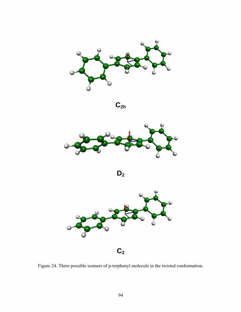
C2h
D2
C2
Figure 24. Three possible isomers of p-terphenyl molecule in the twisted conformation.
94

veral IR absorption peaks abruptly disappear from the spectrum. No hysteresis was
observed in our experiments.
The pressure-dependent shifts of several out-of-plane hydrogen bending modes in
p-terphenyl are plotted in Fig. 27. Again, uncertainties in data are within points’ size. The
frequencies shift discontinuously for certain peaks; namely, the peaks at 567, 573, and
912 cm-1. This observation, together with the disappearance of other peaks, indicates the
existence of a phase transition. The transition pressure lies between 0.2 and 0.6 GPa,
consistent with previous studies (Ref. 65), which determined a phase transition at
approximately 0.5 GPa.
95
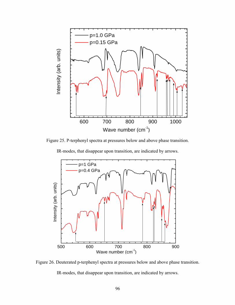
600 700 800 900 1000
p=1.0 GPa p=0.15 GPa
Inte
nsity
(arb
. uni
ts)
Wave number (cm-1)
Figure 25. P-terphenyl spectra at pressures below and above phase transition.
IR-modes, that disappear upon transition, are indicated by arrows.
500 600 700 800 900
p=1 GPa p=0.4 GPa
Inte
nsity
(arb
. uni
ts)
Wave number (cm-1)
Figure 26. Deuterated p-terphenyl spectra at pressures below and above phase transition.
IR-modes, that disappear upon transition, are indicated by arrows.
96

0 1 2 3 4 5 6550
555
560
565
570
575
Wav
e nu
mbe
r (cm
-1)
Pressure (GPa)
Figure 27. Frequency dependence of several IR-modes on the pressure for p-terphenyl.
Table V. Ground-state energies of p-terphenyl molecules in different conformations
relative to the planar conformation.
Energy, meV
Basis set Symmetry
group 6-31+G(d) 6-311+G(d) 6-311++G(2d,p) 6-311++G(2df,2dp)
Planar, D2h 0 0 0 0
Twisted, C2h -163.4 -175.6 -178.7 -146.6
Twisted, D2 -162.4 -174.2 -176.2 -145.4
97
6.1.2.2. Numerical calculations.
Previous theoretical studies have investigated the conformation of the p-terphenyl
molecule (Ref. 58, 91). We performed ab initio calculations of p-terphenyl using the
Gaussian98 software package (Ref. 9). All calculations were done using the same method
as in the case of biphenyl. We used two basis sets, 6-31+G(d) and 6-311+G(d), to obtain
vibrational frequencies for the p-terphenyl molecule in different configurations. In
addition, two higher basis sets, 6-311++G(2d,p) and 6-311++G(2df,2dp) were used to
check the consistency of the ground-state energy calculations. A summary of the energy
calculations is given in Table V. It is clear that the C2h isomer is consistently more
energetically favorable than the D2 isomer. This result is consistent with previous x-ray
diffraction experiments, which indicated that the molecules in a p-terphenyl crystal have
C2h symmetry at low temperatures (Ref. 47). The calculated energy difference, however,
is only ~1 meV/molecule. Our results contradict those obtained in Ref. 58, where it was
suggested that the D2 isomer has a lower energy than the C2h isomer. One possible reason
for such a discrepancy is that in Ref. 58, a semiempirical method was used (CS-INDO),
which is usually less accurate than ab initio methods. Finally, we note that the C2
structure was unstable - during our calculations it relaxed to the 2C′ conformation.
98

6.1.2.3. Group theory.
Similar to the analysis made for biphenyl, we applied group theory to analyze the
normal modes of p-terphenyl. This analysis was performed for the three possible
conformations shown in Fig. 24, as well as the planar conformation.
In the case of D2 symmetry, the vibrational modes are classified as follows:
Γ = 22A ⊕ 20B1 ⊕ 24B2 ⊕24B3 .
Modes belonging to the B1, B2, or B3 irreducible representations are IR-active, for a total
of 68 IR-active modes. For the C2h group, the vibrational modes are classified as:
Γ = 21Ag⊕ 24Bg⊕ 21Au⊕ 24Bu .
Here, only modes belonging to either Au or Bu representations are IR-active, yielding a
total of 45 IR-active modes. For the molecule belonging to C2 point group, the modes are
given by:
Γ = 42A⊕ 48B .
In this case, all modes are IR-active. For the planar configuration, p-terphenyl belongs to
the D2h point group. The vibrational modes are given by:
Γ = 16Ag ⊕ 6Au ⊕ 5B1g ⊕ 15B2g ⊕ 9B3g ⊕ 15B1u ⊕ 9B2u ⊕15B3u .
Modes belonging to the B1u, B2u, or B3u irreducible representations are IR-active, for a
total of 39 IR-active modes.
Upon planarization, certain IR-active peaks become IR-forbidden. We would
expect to see 6 modes disappear from the spectrum if p-terphenyl belongs to the C2h
group, 29 modes if it belongs to the D2 group, and 51 modes if the molecule has C2
symmetry. These “disappearing peaks” comprise a special subset of vibrational modes. In
99

the following discussion, we restrict the analysis to those modes that lose IR activity
upon planarization.
6.1.2.4. Comparison between theory and experiment.
In Figure 28 we present all modes that are IR-inactive in the planar conformation,
but become active in the C2h and 2C′ twisted conformations, along with the experimental
results. The calculations showed that some modes, which are IR-active according to
group theory, have essentially zero intensity. We then looked at the isomer, since it
turned out it deviates from C
2C′
2h symmetry only slightly, as the difference in the twist
angles of outer rings is only 0.03°. There is also a distortion of phenyl rings which makes
them non-planar, but this distortion is also very small—the C-C-C-C dihedral angle is
0.04°. Results are also presented for the D2 isomer. The results for (not shown) are
nearly identical to those for D
2C ′′
2.
In Fig. 28 it is apparent that the most intense calculated peak is at 710 cm-1,
consistent with experiment. For the D2 calculations there is also an intense peak at 741
cm-1. In the experimental spectrum, however, there is no disappearing peak near 741 cm-1.
This observation, along with the ground state energy calculations, allows us to conclude
that the p-terphenyl structure is 2C′ . Since the 2C′ conformation deviates from the C2h
conformation only slightly, it is surprising that this small perturbation causes large
increases in the intensities of certain IR peaks. In Fig. 28, for example, the IR mode at
710 cm-1 has zero intensity for the C2h conformation, but it is very intense for the 2C′
conformation.
100
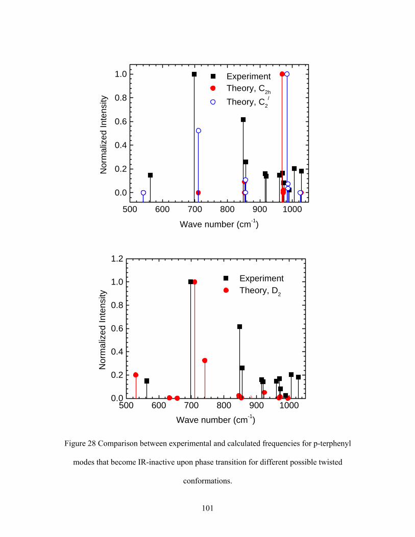
500 600 700 800 900 1000
0.0
0.2
0.4
0.6
0.8
1.0
Experiment Theory, C2h
Theory, C2/
Nor
mal
ized
Inte
nsity
Wave number (cm-1)
500 600 700 800 900 10000.0
0.2
0.4
0.6
0.8
1.0
1.2
Experiment Theory, D2
Nor
mal
ized
Inte
nsity
Wave number (cm-1)
Figure 28 Comparison between experimental and calculated frequencies for p-terphenyl
modes that become IR-inactive upon phase transition for different possible twisted
conformations.
101

500 550 600 650 700 750 800 850 9000.0
0.2
0.4
0.6
0.8
1.0
Experiment Theory, C2h
Theory, C2/
Nor
mal
ized
inte
nsity
Wave number (cm-1)
500 550 600 650 700 750 800 850 9000.0
0.2
0.4
0.6
0.8
1.0
1.2
Experiment Theory, D2
Nor
mal
ized
inte
nsity
Wave number (cm-1)
Figure 29 Comparison between experimental and calculated frequencies for deuterated p-
terphenyl modes that become IR-inactive upon phase transition for different possible
twisted conformations.
102
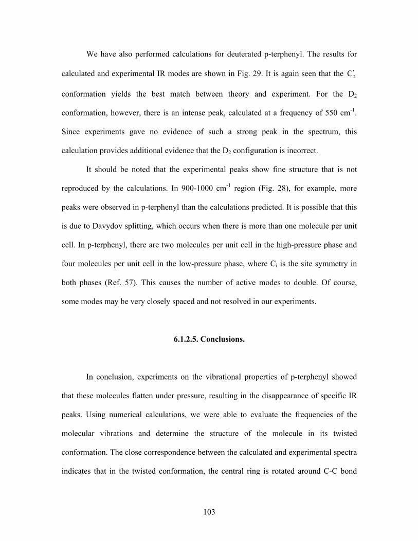
We have also performed calculations for deuterated p-terphenyl. The results for
calculated and experimental IR modes are shown in Fig. 29. It is again seen that the 2C′
conformation yields the best match between theory and experiment. For the D2
conformation, however, there is an intense peak, calculated at a frequency of 550 cm-1.
Since experiments gave no evidence of such a strong peak in the spectrum, this
calculation provides additional evidence that the D2 configuration is incorrect.
It should be noted that the experimental peaks show fine structure that is not
reproduced by the calculations. In 900-1000 cm-1 region (Fig. 28), for example, more
peaks were observed in p-terphenyl than the calculations predicted. It is possible that this
is due to Davydov splitting, which occurs when there is more than one molecule per unit
cell. In p-terphenyl, there are two molecules per unit cell in the high-pressure phase and
four molecules per unit cell in the low-pressure phase, where Ci is the site symmetry in
both phases (Ref. 57). This causes the number of active modes to double. Of course,
some modes may be very closely spaced and not resolved in our experiments.
6.1.2.5. Conclusions.
In conclusion, experiments on the vibrational properties of p-terphenyl showed
that these molecules flatten under pressure, resulting in the disappearance of specific IR
peaks. Using numerical calculations, we were able to evaluate the frequencies of the
molecular vibrations and determine the structure of the molecule in its twisted
conformation. The close correspondence between the calculated and experimental spectra
indicates that in the twisted conformation, the central ring is rotated around C-C bond
103
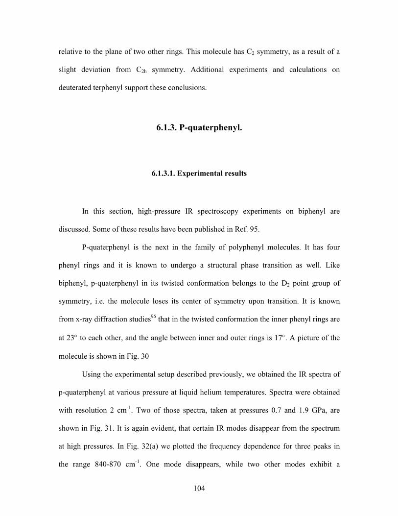
relative to the plane of two other rings. This molecule has C2 symmetry, as a result of a
slight deviation from C2h symmetry. Additional experiments and calculations on
deuterated terphenyl support these conclusions.
6.1.3. P-quaterphenyl.
6.1.3.1. Experimental results
In this section, high-pressure IR spectroscopy experiments on biphenyl are
discussed. Some of these results have been published in Ref. 95.
P-quaterphenyl is the next in the family of polyphenyl molecules. It has four
phenyl rings and it is known to undergo a structural phase transition as well. Like
biphenyl, p-quaterphenyl in its twisted conformation belongs to the D2 point group of
symmetry, i.e. the molecule loses its center of symmetry upon transition. It is known
from x-ray diffraction studies96 that in the twisted conformation the inner phenyl rings are
at 23° to each other, and the angle between inner and outer rings is 17°. A picture of the
molecule is shown in Fig. 30
Using the experimental setup described previously, we obtained the IR spectra of
p-quaterphenyl at various pressure at liquid helium temperatures. Spectra were obtained
with resolution 2 cm-1. Two of those spectra, taken at pressures 0.7 and 1.9 GPa, are
shown in Fig. 31. It is again evident, that certain IR modes disappear from the spectrum
at high pressures. In Fig. 32(a) we plotted the frequency dependence for three peaks in
the range 840-870 cm-1. One mode disappears, while two other modes exhibit a
104

discontinuity in the slope of the frequency versus pressure plots. This is an indication of
the phase transition. In Fig. 32(b) we provide further evidence for the presence of a phase
transition. In this plot the area of the peak at 864 cm-1 was normalized with respect to the
area of the peak at 860 cm-1 and plotted as a function of pressure. It is seen that the
normalized area is zero within experimental uncertainty after the phase transition. The
increase in the normalized area before the phase transition is due to the decrease in the
area of the peak at 860 cm-1.
6.1.3.2. Group theory.
Group-theoretical analysis of the vibrational modes of p-quaterphenyl yields the
following results
321vibr B32B32B27A29 ⊕⊕⊕=Γ
for the twisted conformation of the molecule. Modes that belong to B1, B2, and B3
representations are IR-active. For the planar conformation we have:
u3u2u1
g3g2g1ugvibr
B12B20B20
B20B12B7A8A21
⊕⊕⊕
⊕⊕⊕⊕=Γ .
Here the modes belonging to B1u, B2u, and B3u representations are IR-active. Thus in the
planar conformation there are 52 IR-active modes and there are 91 IR-active modes in the
twisted conformation. Therefore, some IR absorption peaks should disappear upon
transition from the twisted to the planar conformation, in agreement with our
observations.
105
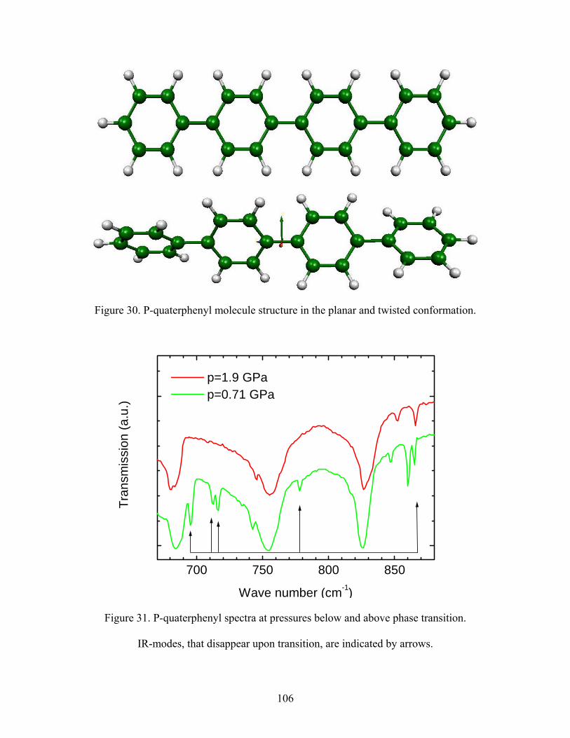
Figure 30. P-quaterphenyl molecule structure in the planar and twisted conformation.
700 750 800 850
p=1.9 GPa p=0.71 GPa
Tran
smis
sion
(a.u
.)
Wave number (cm-1)
Figure 31. P-quaterphenyl spectra at pressures below and above phase transition.
IR-modes, that disappear upon transition, are indicated by arrows.
106

0.0 0.5 1.0 1.5 2.0 2.5 3.0
850
860
870 (a.)
Wav
e nu
mbe
r (cm
-1)
Pressure (GPa)
0.0 0.5 1.0 1.5 2.0 2.5 3.0
0.0
0.2
0.4
0.6(b.)
Nor
mal
ized
are
a
Pressure (GPa)
Fig. 32. Frequency dependence of several IR-modes on the pressure for p-
quaterphenyl and normalized area dependence on the pressure for an IR-mode that
become IR-inactive upon phase transition for p-quaterphenyl molecule.
107
The reason that we do not observe 39 disappearing peaks is probably due to the
fact that some modes may be too weak to be observed, and others may be not resolved
from neighboring peaks. In the 600-900 cm-1 region, which corresponds to the hydrogen
out-of-plane bending modes, we observe five disappearing peaks. According to the
group-theory analysis (not shown) there will be 9 IR modes, which disappear from the
spectrum. But since four of them belong to B1 representation and have the dipole
moments induced to be very small, they may be too weak to be either resolved or
detected. Thus we are left with five modes belonging to the B3 representation, which
become of B3g representation and, therefore, lose IR-activity upon planarization of the
molecule. In Fig. 34 we presented comparison between experimental and calculated
frequencies of the modes that become IR-inactive upon the phase transition. The
agreement is not as good as it was for biphenyl. It tends to become worse with the
increase in the molecule size. The theory though also predicts five modes in the range
from 600 to 900 cm-1 to disappear upon planarization of p-quaterphenyl molecule.
6.1.3.3. Conclusions.
In conclusion, the second-order phase transition was observed in p-quaterphenyl,
as was for biphenyl and p-terphenyl. The critical pressure is about 0.9 GPa. The molecule
becomes planar upon such a transition, which results in the disappearance of several IR
peaks from the spectrum. Spectra are reproducible and no hysteresis behavior was found.
108
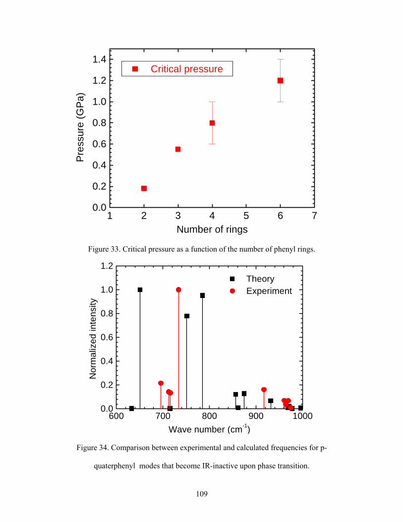
1 2 3 4 5 6 70.0
0.2
0.4
0.6
0.8
1.0
1.2
1.4
Critical pressureP
ress
ure
(GP
a)
Number of rings
Figure 33. Critical pressure as a function of the number of phenyl rings.
600 700 800 900 10000.0
0.2
0.4
0.6
0.8
1.0
1.2
Theory Experiment
Nor
mal
ized
inte
nsity
Wave number (cm-1)
Figure 34. Comparison between experimental and calculated frequencies for p-
quaterphenyl modes that become IR-inactive upon phase transition.
109
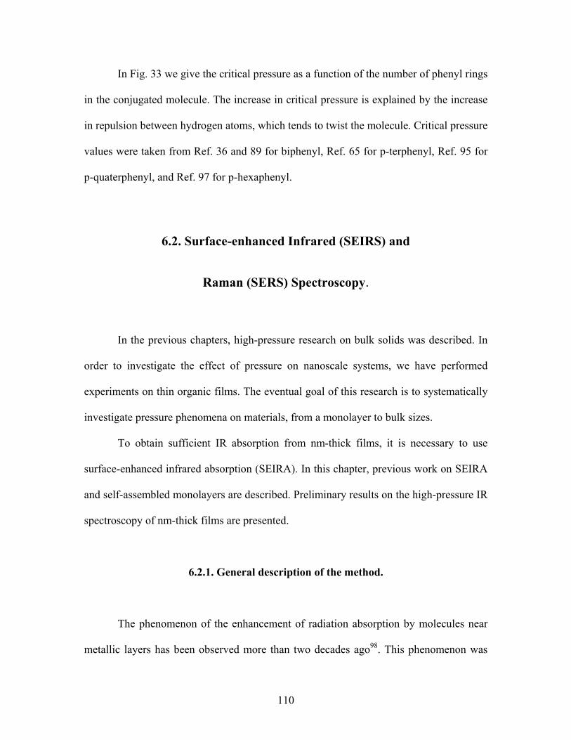
In Fig. 33 we give the critical pressure as a function of the number of phenyl rings
in the conjugated molecule. The increase in critical pressure is explained by the increase
in repulsion between hydrogen atoms, which tends to twist the molecule. Critical pressure
values were taken from Ref. 36 and 89 for biphenyl, Ref. 65 for p-terphenyl, Ref. 95 for
p-quaterphenyl, and Ref. 97 for p-hexaphenyl.
6.2. Surface-enhanced Infrared (SEIRS) and
Raman (SERS) Spectroscopy.
In the previous chapters, high-pressure research on bulk solids was described. In
order to investigate the effect of pressure on nanoscale systems, we have performed
experiments on thin organic films. The eventual goal of this research is to systematically
investigate pressure phenomena on materials, from a monolayer to bulk sizes.
To obtain sufficient IR absorption from nm-thick films, it is necessary to use
surface-enhanced infrared absorption (SEIRA). In this chapter, previous work on SEIRA
and self-assembled monolayers are described. Preliminary results on the high-pressure IR
spectroscopy of nm-thick films are presented.
6.2.1. General description of the method.
The phenomenon of the enhancement of radiation absorption by molecules near
metallic layers has been observed more than two decades ago98. This phenomenon was
110

called surface-enhanced infrared absorption (SEIRA) and has become a very powerful
method for studying chemical contaminants and molecular monolayers. Substantial
research effort has been made to study SEIRA. Among the organic chemical compounds
the most studied include p-nitrothiophenol99,100, disulfide and diselenide molecules101,
dichalogenide molecules102, and p-nitrobenzoic acid103, ,104 105. Inorganic compound have
also been studied by this technique106,107. In all these studies it has been found that the IR-
absorption greatly (103-104 times) increases for certain IR-modes if the molecule is
located near the metallic layer. The metals that show the most prominent enhancement
are silver (Ag), lead (Pb), platinum (Pt), gold (Au), and copper (Cu). Not all modes are
enhanced equally, which indicate the selective character of this process. A detailed
review of the SEIRA can be found in Ref. 108.
It is now generally accepted that there are three major mechanisms that contribute
to the total enhancement: electromagnetic, chemical, and orientational mechanisms. The
orientational mechanism is the simplest and is due to the fact that the absorption of light
is proportional to , where θ2cos θ is the angle between the dipole moment derivative
with respect to normal coordinate and the electric field of the incident radiation. Since the
space average of is 1/3, the orientational mechanism can provide an enhancement
by a factor of three at most. The chemical mechanism of enhancement involves the
chemical interaction between the molecule and the metal surface. It is known that
chemisorbed molecules absorb stronger than physisorbed ones. It is believed that the
charge transfer from the metal to the molecule contributes to enhancement, and some
experiments seem to support this theory
θ2cos
109, ,110 111.
111
The electromagnetic mechanism of IR-absorption enhancement has been very
extensively studied from both experimental and theoretical point of
view112, , , , , , , ,113 114 115 116 117 118 119 120. It is now generally accepted that the excitation of
plasmons in metal and their coupling with molecular vibrations is the main mechanism
for the electromagnetic enhancement of IR- and Raman signal. The enhancement greatly
depends on the metal surface morphology121, which indicates that the surface structure is
the important factor in achieving larger enhancements. Below we consider the
electromagnetic mechanism in more detail, following the review given in Ref. 120.
6.2.2. Electromagnetic (EM) mechanism of surface-enhanced absorption.
If electromagnetic radiation impinges onto the metal surface, the local field near
the surface is different from the field far away from it. In practice, the metal surface is
usually rough and the roughness size varies from nanometers to microns. We are
interested in the metals deposited from the vapor or by a sputtering process, where the
size of the metal particles is 1-100 nm. In this case the particle size is much smaller than
the wavelength of radiation. In this case the electric field can be assumed to be uniform,
but varying in time. The retardation effects can all be neglected and the polarization of
the spherical metal particle is determined by a well-known result:
EPrr
ε+εε−ε
ε=2
3met
met , (113)
where and are dielectric constants of surrounding medium and the metal,
respectively. The case of non-spherical particles will be addressed later.
ε metε
112

The polarization given by Eq. (113) corresponds to the dipole moment
Pprr 3a
34
π= , where a is the radius of the sphere. The electric dipole field is then given by:
( )( ) [ ]
⎭⎬⎫
⎩⎨⎧
⎟⎠⎞
⎜⎝⎛ −−⋅+××
ε+εε−ε
επ=ω−
rik
r1ˆ)ˆˆ(ˆ3ˆˆˆkE
r)2(e)(a4 2
20
met
tkrimet3
dip eennnenEr
(114)
Here is the unit polarization vector of the incident radiation (not to be confused with
the polarization of the metal particle from Eq. (113)!), r is the radial distance from the
center of the spherical particle,
e
rˆ rn
r
= is the unit vector in the direction of rr , and k is the
wave vector of the incident radiation.
Eq. (114) already enables us to understand the mechanism of surface-
enhancement. If the dielectric constant of the metal has small imaginary part and real part
equal to -2ε, the electric field given by Eq. (114) becomes very large. The absorption and
scattering intensities are proportional to the square of the electric field and thus become
very large too. The total electric field is the sum of the incident and scattered fields and
can be written as:
[ ] )tkr(i023
2
dipinctot eErik
r1ˆ)ˆˆ(ˆ3ˆ)ˆˆ(
rkˆ ω−
⎟⎟⎠
⎞⎜⎜⎝
⎛
⎭⎬⎫
⎩⎨⎧
⎟⎠⎞
⎜⎝⎛ −−⋅+××η+=+= eennneneEEE
rrr (115)
where ε+ε
ε−εεπ=η
2a4
met
met3 and E0 is the amplitude of the incident electric field.
The more realistic model of the experiments on surface-enhanced spectroscopy is
the collection of spheres coated with the layer of material under investigation. As the
first-order approximation one can assume that all spheres are of the same radius and the
spacing between spheres is much larger than the sphere radius. In this case each sphere
can be considered independently and the problem reduces to the two-layered sphere in
113

the uniform electric field. The problem is exactly solvable and the final result gives the
electric field outside the sphere in the form:
⎭⎬⎫
⎩⎨⎧ −⋅
⎥⎦
⎤⎢⎣
⎡⎟⎠⎞
⎜⎝⎛
+ε−ε
+= 3310 r
ˆ)ˆˆ(ˆ321RˆE znznzE
r (116)
where R1 is the radius of the outer coating layer surface, r is the radius-vector, and ε is
the so-called effective medium dielectric constant. The value of ε is given by:
( )( ) ( )⎥⎦
⎤⎢⎣
⎡ε−ε−ε+ε
ε−ε+ε=ε
1212
121 f2
f31 (117)
where and are dielectric constants of the coating layer and the inner spherical
particle, respectively,
1ε 2ε
VV
RRf sphere
31
32 == is the filling factor, and R2 is the inner sphere
radius. The Eq. (117) coincides with the famous result of Maxwell-Garnett theory122
(MGT) for small spherical particles with dielectric constant 2ε embedded in the medium
with dielectric constant . The condition in MGT that the spheres can be considered
independently requires the filling factor to be small. In our case the spacing between
spherical particles must be large compared to their size. In this case the influence of one
sphere onto another can be neglected.
1ε
Since the composite medium was treated as the homogeneous medium with
effective dielectric constant, the theory described is effective medium theory (EMT).
Another EMT is the Bruggeman theory123. More detailed review can be found in Ref.
108, 114.
Alternative theories have also been developed124, ,111,118125 . In those theories the
metal particles and the molecules are replaced by polarizable dipoles The magnitudes
of the dipoles are determined via the following coupled dipoles (CD) equation:
ipr
114

⎟⎟⎠
⎞⎜⎜⎝
⎛+α= ∑
≠ijjij0ii M pEprrr . (118)
Here is the polarizability of the iiα th dipole and Mij describes the interaction between the
ith and jth dipoles. The value of Mij is given by the second term in parentheses in Eq. (115)
where the vector r must be replaced by r
ijrr , the vector from the ith to jth dipole position.
The Eq. (118) must be solved self-consistently. Recent calculations showed good
agreement between experimental and computed data, as well as consistency among
different theories126,118,119,120.
All models considered above have implicitly assumed that the particles are big
enough to be treated as macroscopic medium with dielectric constant determined for such
a medium. It is known, however, that the dielectric constant becomes size dependent for
very small particles. In fact, the size dependence manifests itself when the size of the
particle becomes comparable to the mean free path of conducting electrons. This changes
the plasmon width and, for spherical particles, can be described by the following relation :
RvA F
b +γ=γ , (119)
where is Fermi velocity and R is the radius of the sphere. Coefficient A in Eq. (119) is
equal to 1 in classical theory and ranges from 0.76 to 1.16 in various quantum-
mechanical models
Fv
127,128. The detailed review on this subject can be found elsewhere .
115

6.3. Thin films of organic molecules under pressure.
Thin molecular and atomic films and self-assembled monolayers (SAM) have
recently become a subject of intensive scientific research. They have been studied
experimentally by atomic force microscopy129, ,130 131 (AFM), scanning tunneling
microscopy132, , ,133 134 135 (STM), X-ray diffraction136, , ,137 138 139, transmission electron
microscopy , x-ray photoelectron spectroscopy140,141 (XPS), sum-frequency generation142
(SFG), surface second harmonic generation143,144 (SSHG), Brewster angle microscopy145,
ellipsometry146,140,141, Raman scattering147, infrared (IR)
spectroscopy133,134,135, , , , ,141148 149 150 151 , and theoretically by molecular dynamics
simulations152, , ,153 154 155.
It is known that thiol molecules form layered structures on different substrates
such as metal surfaces, silicon, and glasses. The most studied are alkenethiol,
benzenethiol, thiophenol and some others. The most frequently used substrate is gold
(Au). The alkenethiol molecules deposited on Au(111) can form ( ) o30R33 × or 11×
structures. The application of surface pressure drives the transition and hysteresis was
observed. The ( ) o30R33 × structure persists up to a load of 280 nN and then 11×
structure appears. Upon decreasing the load the ( ) o30R33 × structure reappears only
at a load about 100 nN. The global phase diagram of n-alkenethiol SAM has been
investigated and two regimes have been found: long (n>14) and short ( ) chain-
length regimes. Different phases are characterized by the tilt direction and two-
dimensional periodicity. The tilt angle was found to be about 30-35° from normal to the
surface
12n ≤
136,148. The molecular dynamics simulations showed that there are two phase
116
transitions in SAM of alkylthiol molecules: one is a change in tilt direction from nearest
neighbor (NN) to next-nearest neighbor (NNN) and another is a transition from NNN tilt
to an orientationally disordered state. A similar transition was found in the SAM of
azobenzene derivative, 4-octyl- 4′ -(carboxytrimethyleneoxy)azobenzene (C8AzoC3) . The
low-pressure phase has the tilt toward NN whereas high-pressure phase has the tilt
toward NNN. It was found that the tilt angle does not change much with pressure.
Pyridine molecules on Au(111) form various structures with flat-lying, tilted, and
vertically standing molecules . In this case the tilt angle varies from 20 to 45° and
increases as the applied surface potential or surface concentration increases. The same
group of researchers studied 2, 2 -bypyridine (bpy) SAM and found two phase transitions
as applied potential increases. One transition is from flat to vertically oriented molecules
and another one is from
′
343× zigzag to 324× commensurate structure.
Another large group of thiol molecules, which form SAMs, are aromatic
molecules. The simplest molecule is benzenethiol. It forms a well-ordered monolayer
with a ( ) o9.13R1313 × commensurate structure . As shown by STM and surface-
enhanced infrared absorption (SEIRA), the phenyl ring is tilted about 30° from surface
normal. Also p-biphenyl mercaptan (BPM) and p-terphenyl mercaptan (TPM) have been
studied and it was determined that they form stable monolayers with reproducible contact
angles . The structure of these monolayers is ( ) o30R33 × and molecules are almost
perpendicular to substrate surface.
The pressure effect on thin films has been also investigated. In Ref. 147 it was
found that in the polydiacetylene the phonon frequencies increase, but the Raman
frequencies shift to the red part of the spectrum. This behavior was attributed to the
117

increase of conjugation length with pressure. In 1,2-dipalmitoyl-sn-glycero-3-
phosphocholine (DPPC) the surface pressure application leads to the increase in
frequency of C-H vibrations and in the signal intensity . These findings, as will be seen
below, are consistent with our own observations.
6.4. Current research.
6.4.1. Film preparation.
A silver film was deposited onto the culet surface of the diamonds in the DAC by
the vapor deposition method. The scheme of the deposition system is shown on Fig. 35.
The DAC was placed into the deposition chamber and the chamber was evacuated to
about 10-7-10-9 Torr. First, the roughing pump brought pressure down to 100 Torr. Then
the cryopump was opened to the ambient atmosphere and heated up to 500° C. After
several hours of heating it was isolated from the atmosphere and cooled down to liquid
nitrogen temperature (77 K). When thermal equilibrium was reached, the valve,
connecting the cryopump with the deposition chamber, was opened and the pressure
decreased to a level of ~1 mTorr. The final stage involves the ion pump evacuating the
whole chamber. The valve between the ion pump and the chamber was slowly opened
and the pressure in the ion pump was monitored and not allowed to exceed 10-5 Torr. The
filaments of the ion pump operated with ~50 A current in continuous or 2-5 minute cycle
mode. It usually takes 1-2 hours for the ion pump to bring the pressure down to the values
mentioned above. During the operation the ion pump must be cooled by a continuous
118
water flow. The deposition current can vary in the range 175-250 A and the rate of silver
deposition varies in a wide range from 0.1 to 100 Å/s. A manually operated shutter
allows one to control the deposition time and, thus, the film thickness. In order to monitor
the thickness correctly the deposition rate should not exceed 5 Å/s. However, the higher
the deposition rate, the rougher the film surface is, which is important for the surface
enhanced spectroscopy.
For the purpose of SEIRA measurements the silver film thickness must be small
enough in order not to block the infrared light passing through the diamonds. At the same
time the film must provide sufficient enhancement of the IR absorption so that the IR
detector receives sufficient signal. Usually the film thickness is about 10 nm for good
enhancement, but we have used a 5 nm thick film to get a good signal to noise ratio.
Since the enhancement is greater for a film with rougher surface profile, we chose a
deposition rate of about 5 Å/s.
Thin film of p-NTP has been casted from the solution onto the silver layer
covering diamond surface. This technique of organic thin film preparation has been
described elsewhere . In order to protect the epoxy, which glues diamonds to the backing
plates, from the chemical solution we put additional layer of epoxy after silver film
deposition. The AFM images of p-NTP thin film have been taken after a series of high-
pressure experiments (Appendix D). They showed a film of about 30 nm thick (Fig. 38,
39). Large white features in the image are dust particles and small ruby chunks, which are
inevitably introduced in the loading process.
119
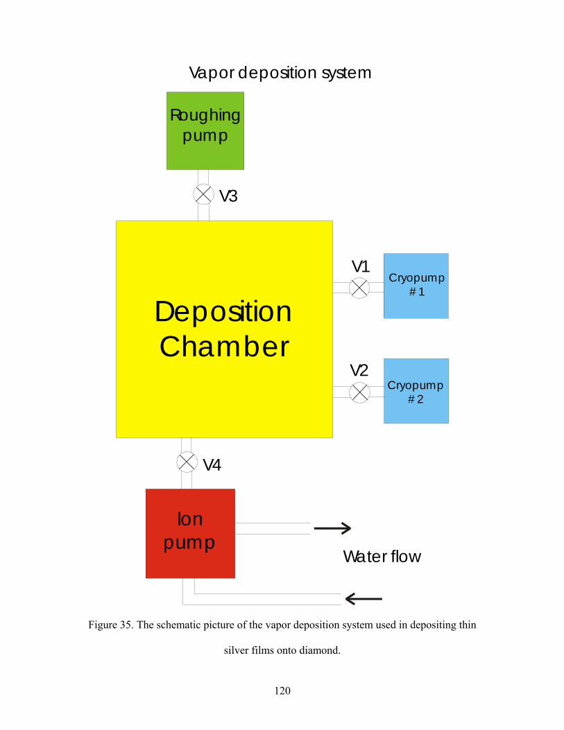
Roughing pump
Cryopump# 1
Cryopump# 2
Ionpump
Water flow
V1
V2
V3
V4
DepositionChamber
Vapor deposition system
Figure 35. The schematic picture of the vapor deposition system used in depositing thin
silver films onto diamond.
120

A more detailed structure could be possibly obtained by STM measurements,
which we didn’t perform. The deposited film has been loaded with liquid nitrogen in the
DAC with type II diamonds and FT-IR spectra have been taken. The pressure was
calibrated using ruby fluorescence method. For this purpose the tiny ruby chip was placed
on top of the film. The introduction of the ruby chip inevitably damages the thin film. In
our case, however, the size of the chip was negligible compared to the sample size. Thus
no significant damage to the film has been done.
6.4.2. Results.
Typical spectra of the thin p-NTP film are shown in Fig. 36. The broad peak at
1340 cm-1 corresponds to a symmetric stretch of NO2 group in the p-NTP molecule.
Spectra have been obtained at the room temperature with an MCT detector. The spectral
resolution was 8 cm-1. In the Fig. 37 we present peak frequency as a function of pressure.
The frequency shifts up with pressure, though the apparent shift is smaller than the
resolution. Thus no certain conclusions can be drawn about its behavior now and a more
sensitive technique is required. Nevertheless, the pressure seems to affect the film
significantly enough so that IR-spectroscopy can serve as a probe of film behavior under
high pressures. Upon decrease of the pressure the peak intensity went down, which made
it hard to detect the peak at pressures between 1 and than 5 GPa. But then the intensity is
increased at the pressures below 1 GPa. Whether it is due to a phase transition in the
nitrogen, which occurs at 1.9 GPa, is currently not known.
121

1320 1330 1340 1350 1360
2.8
3.0
3.2
3.4
p=1.9 GPa p=0 GPa p=6.3 GPa
Tran
smis
sion
(arb
. uni
ts)
Wave number (cm-1)
Figure 36. Typical IR spectra of p-NTP film at different pressures.
0 1 2 3 4 5 6 71341
1342
1343
1344
1345
1346
1347
1348
Wav
e nu
mbe
r (cm
-1)
Pressure (GPa)
Figure 37. Pressure dependence of NO2 symmetrical stretch mode
frequency in p-NTP film.
122

Overall, application of the pressure to thin films seems to influence the vibrational
frequencies of the molecules composing the film and can serve as a good probe of the
film properties. Much of the research has to be done in this area and a lot of discoveries
are still waiting to be made.
7. Summary of results
In this work the following results have been obtained:
• High pressure can be applied to the study of organic solids and thin films of
organic materials;
• Biphenyl, p-terphenyl, and p-quaterphenyl all undergo structural phase transitions
when pressure increases above certain critical value;
• Several IR modes become inactive upon this transition;
• The critical pressure increases with the number of phenyl rings;
• Among two possible twisted conformations of p-terphenyl, the conformation
belonging to the C2h symmetry is the most stable;
• Numerical ab initio calculations show very good agreement with experiment;
• Thin films of organic molecules can be successfully studied by means of surface-
enhanced IR absorption method. High pressure affects the thin film properties;
Most of these results have been published in peer-reviewed journals and presented at
various meetings.
123

8. Future work directions
A new branch of research in physics and chemistry is connected with the properties of
self-assembled monolayers. A monolayer provides a model system to study materials
properties on the nanometer length scale. Those materials should exhibit interesting
mechanical, optical and other physical properties. Quasi-two-dimensional systems can
lead to discoveries of new phenomena. Pressure-induced phase transitions in such
systems might be a good test for existing theoretical models, such as Ising or Potts
models, which have been successfully applied to various surface phenomena156, and a
way to develop new, more sophisticated models to describe behavior of two-dimensional
systems. Pressure in this case can also be a very powerful tool to probe atomic
interactions between monolayer molecules. I have been studying pressure effects on p-
nitrothiophenol monolayers grown on metallic substrates by means of infrared (IR)
spectroscopy. There exists several surface characterization techniques, such as scanning
tunneling microscopy (STM), atomic force microscopy (AFM), and surface second
harmonic generation (SSHG), to study the effects of high pressure.
High pressure can be a very useful characterization tool for the investigation of
the thin films. By systematically increasing the thickness of the film, one can probe bulk
vs. surface properties of a material. By monitoring changes in the material’s response to
applied pressure with increasing thickness, one can find out when this material starts
exhibiting bulk behavior. IR spectroscopy can provide a direct indication to some
changes within the material. The research in this area can lead to a deeper understanding
of the structure of different substances and may result in discoveries of novel materials.
124
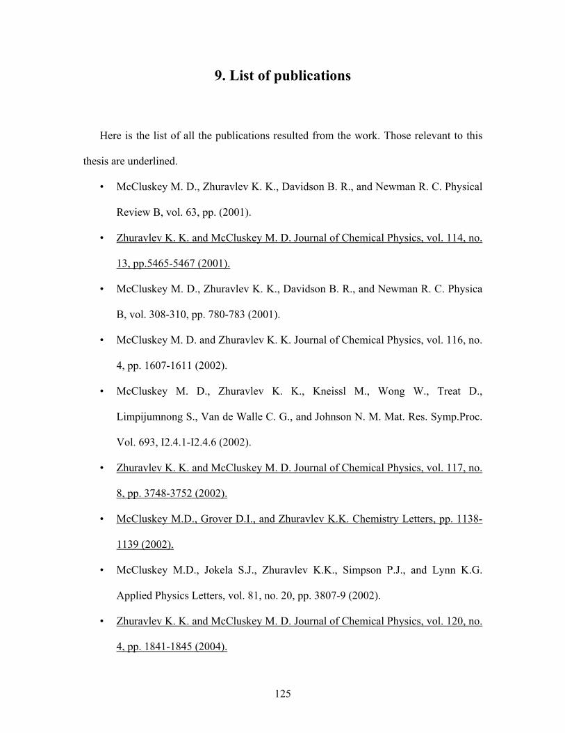
9. List of publications
Here is the list of all the publications resulted from the work. Those relevant to this
thesis are underlined.
• McCluskey M. D., Zhuravlev K. K., Davidson B. R., and Newman R. C. Physical
Review B, vol. 63, pp. (2001).
• Zhuravlev K. K. and McCluskey M. D. Journal of Chemical Physics, vol. 114, no.
13, pp.5465-5467 (2001).
• McCluskey M. D., Zhuravlev K. K., Davidson B. R., and Newman R. C. Physica
B, vol. 308-310, pp. 780-783 (2001).
• McCluskey M. D. and Zhuravlev K. K. Journal of Chemical Physics, vol. 116, no.
4, pp. 1607-1611 (2002).
• McCluskey M. D., Zhuravlev K. K., Kneissl M., Wong W., Treat D.,
Limpijumnong S., Van de Walle C. G., and Johnson N. M. Mat. Res. Symp.Proc.
Vol. 693, I2.4.1-I2.4.6 (2002).
• Zhuravlev K. K. and McCluskey M. D. Journal of Chemical Physics, vol. 117, no.
8, pp. 3748-3752 (2002).
• McCluskey M.D., Grover D.I., and Zhuravlev K.K. Chemistry Letters, pp. 1138-
1139 (2002).
• McCluskey M.D., Jokela S.J., Zhuravlev K.K., Simpson P.J., and Lynn K.G.
Applied Physics Letters, vol. 81, no. 20, pp. 3807-9 (2002).
• Zhuravlev K. K. and McCluskey M. D. Journal of Chemical Physics, vol. 120, no.
4, pp. 1841-1845 (2004).
125
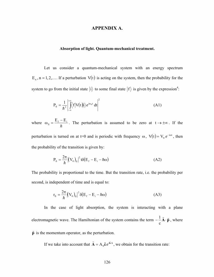
APPENDIX A.
Absorption of light. Quantum-mechanical treatment.
Let us consider a quantum-mechanical system with an energy spectrum
. If a perturbation K,,, 21nE n = ( )tV is acting on the system, then the probability for the
system to go from the initial state i to some final state f is given by the expression4:
( )2
ti2fi dtitVf1P fi∫
+∞
∞−
ω= eh
(A1)
where h
iffi
EE −=ω . The perturbation is assumed to be zero at . If the
perturbation is turned on at t=0 and is periodic with frequency
±∞→t
ω , , then
the probability of the transition is given by:
( ) ti0VtV ω−= e
( ) ( ω−−δπ
= hh
if2
fi0fi EEtV2P ) (A2)
The probability is proportional to the time. But the transition rate, i.e. the probability per
second, is independent of time and is equal to:
( ) ( ω−−δπ
= hh
if2
fi0fi EEV2r ) (A3)
In the case of light absorption, the system is interacting with a plane
electromagnetic wave. The Hamiltonian of the system contains the term pA rr⋅−
c1 , where
pr
is the momentum operator, as the perturbation.
If we take into account that xkεArrr
⋅= i0A eˆ , we obtain for the transition rate:
126

( )( )( ) ( ω−−δ⋅π
= ⋅ω hr
h
r
if
2
fici2
o2fi EEAc
2r pεxn ˆe ˆ )
]
. (A4)
When the wavelength of the incident light is much greater than the size of the system, the
exponential in Eq. (A4) can be replaced by 1. This is the so-called electric dipole (or E1)
approximation. Assuming that the initial state is the ground state, and using the
commutation relation [ 0Hi rp rr−= , where H0 is the unperturbed Hamiltonian, one obtains
for the absorption rate from the ground state:
( ) ( ω−ωδ⋅πω
= 0f
2
fi2o22
20f
fi Ac
2r dε
r
hˆ ) , (A5)
where is the dipole moment of the system. Thus the absorption rate is proportional to
the square of the matrix element of the dipole moment.
dr
127

APPENDIX B.
Isotopic shift of the vibrational frequency of the molecule.
Let us consider the simplest case of a diatomic molecule consisting of two
different atoms with masses and , where superscript (0) is referred to the isotope
type. The chemical bond between these atoms is described, in the harmonic
approximation, by a force constant . The vibrational frequency is given by:
)0(1m 2m
k
( ) ( ) 12
1)0(1
10 mm;k −−− +=µµ=ω (B1)
If one of the atoms is replaced by its isotope with the mass , the vibrational
frequency changes and becomes:
)1(1m
( ) ( ) 12
1)1(1
11 mm;k −−− +=µ′µ′=ω (B2)
The ratio of two frequencies is given by:
( ) ( )( ) ( ) 1
21)0(
1
12
1)1(1
0
1
mm
mm−−
−−
+
+=
µ′µ
=ωω (B3)
It is seen from B3 that if we replace the atom with its lighter isotope ( ), the
frequency is blue-shifted. If the isotope is heavier, the frequency will be red-shifted.
)0(1
)1(1 mm <
The most interesting case is when one of the atoms is hydrogen. The hydrogen
atom is much more lighter that almost any other atom and in this case the ratio 2
)0(1
mm
is small. In the case when hydrogen is replaced by deuterium, the ratio of the frequencies
is approximately equal to:
128

21
mm
)1(1
)0(1
0
1 =≈ωω (B4)
The frequency is, therefore, red-shifted by a factor of 2 . The real shift is smaller due to
the fact that the second atom has finite mass (correction factor, up to linear terms, is
2m211+ and due to anharmonic effects.
129

APPENDIX C.
Frequency distribution for the system of oscillators
with nearest-neighbor interaction.
Let us consider a chain of identical harmonic oscillators with natural frequency
, interacting with each other. We assume free boundary conditions. The interaction
potential will be chosen as follows:
0ω
⎩⎨⎧ =−α
=otherwise,0
1jiif,xxV ji
ij (C1)
Thus we consider nearest-neighbor interaction only. The total Hamiltonian for such a
system is given by:
∑∑ α+⎟⎟⎠
⎞⎜⎜⎝
⎛ ω+=
= ijji
N
1i
2i
20
2i xx
2xm
m2p
H (C2)
where symbol ij indicates the sum over nearest neighbors. Using Hamilton’s equations
of motion
⎪⎪⎩
⎪⎪⎨
⎧
∂∂
=
∂∂
−=
ii
ii
pHx
xHp
&
&
(C3)
one can readily obtain:
130

⎪⎩
⎪⎨⎧
=
α−α−ω−= +−
mpx
xxxmp
ii
1i1ii20i
&
&
(C4)
Dot above the letter means differentiation with respect to time. From Eq. (C4) we can
obtain N second-order coupled differential equations:
⎪⎪⎪
⎩
⎪⎪⎪
⎨
⎧
α−ω−=
α−α−ω−=
α−α−ω−=
α−ω−=
−
−−−
1NN20N
N2N1N201N
312202
21201
xxmxm
xxxmxm.........................................
xxxmxm
xxmxm
&&
&&
&&
&&
(C5)
The standard way to solve this problem is to find all normal modes of the system. We
assume the solution to have a form and, upon substitution in Eq. (C5), we
get:
ti0ii ex)t(x ω−=
⎪⎪⎪
⎩
⎪⎪⎪
⎨
⎧
=+λ=++λ
=++λ=+λ
−
−−
0xx0xxx
...........................0xxx
0xx
1NN
2NN1N
312
21
(C6)
Here α
ω−ω=λ
)(m 220 . System (C6) has nontrivial solution if its determinant is zero.
Therefore we obtain equation for λ :
0)(Det N =Λ (C7)
where
131
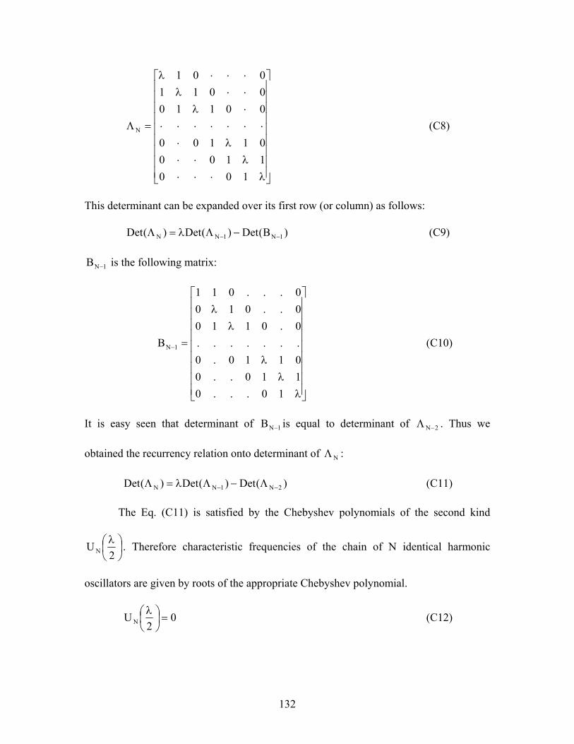
⎥⎥⎥⎥⎥⎥⎥⎥⎥
⎦
⎤
⎢⎢⎢⎢⎢⎢⎢⎢⎢
⎣
⎡
λ⋅⋅⋅λ⋅⋅
λ⋅⋅⋅⋅⋅⋅⋅⋅
⋅λ⋅⋅λ⋅⋅⋅λ
=Λ
100110001100
001100011001
N (C8)
This determinant can be expanded over its first row (or column) as follows:
)B(Det)(Det)(Det 1N1NN −− −Λλ=Λ (C9)
1NB − is the following matrix:
⎥⎥⎥⎥⎥⎥⎥⎥⎥
⎦
⎤
⎢⎢⎢⎢⎢⎢⎢⎢⎢
⎣
⎡
λλ
λ
λλ
=−
10...0110..00110.0.......0.01100..0100...011
B 1N (C10)
It is easy seen that determinant of is equal to determinant of . Thus we
obtained the recurrency relation onto determinant of
1NB − 2N−Λ
NΛ :
)(Det)(Det)(Det 2N1NN −− Λ−Λλ=Λ (C11)
The Eq. (C11) is satisfied by the Chebyshev polynomials of the second kind
⎟⎠⎞
⎜⎝⎛ λ
2U N . Therefore characteristic frequencies of the chain of N identical harmonic
oscillators are given by roots of the appropriate Chebyshev polynomial.
02
U N =⎟⎠⎞
⎜⎝⎛ λ (C12)
132

It is well known fact that these polynomials have simple real roots, lying in the interval
. Thus our system has N distinct frequencies, ranging from [ 1;1− ]m22
0α
−ω to
m22
0α
+ω . In fact, there is a short analytical form for frequencies of the normal modes
of the system. Chebyshev polynomial can be represented as follows: NU
( ) [ ]θ
θ+=θ
sin)1N(sincosU N (C13)
It is zero when the numerator is zero and denominator is not. One can easily obtain:
N...1k,1N
kk =
+π
=θ (C14)
It follows from Eq. (C14) that
⎟⎠⎞
⎜⎝⎛
+π
=λ1N
kcos2k (C15)
Finally, for characteristic frequencies of the system we have:
⎟⎠⎞
⎜⎝⎛
+πα
−ω=ω1N
kcosm22
0k (C16)
In the case of weak coupling the width of distribution of frequencies is of the order of
20m
2ω
α .
If the coupling is such that α 20m
2 ω=α , Eq. (C16) becomes:
⎟⎟⎠
⎞⎜⎜⎝
⎛+
πω=ω
)1N(2ksin2 0k , (C17)
analogously to the dispersion relation for the phonons in crystal.
133

Appendix D.
AFM images of thin film of p-NTP.
Figure 38. AFM image of p-NTP thin film.
134

Figure 39. Section analysis of p-NTP thin film.
135

References:
1E. Schroedinger, Ann. D. Physik 79 486 (1926).
2 D. R. Hartree, Proc. Camb. Phil. Soc. 24 89 (1928).
3 V. Fock, Z. Phys. 61 126 and ibid 62 795 (1930).
4 L. D. Landau and E. M. Lifshits, Quantum mechanics, Nonrelativistic theory, Pergamon
Press, Oxford (1965).
5 P. Hohenberg and W. Kohn, Phys.Rev. B 136 864-870 (1964).
6 W. Kohn and L. J. Sham, Phys. Rev. A 140 1133-1138 (1965).
7 W. Kohn, Rev. Mod. Phys. 71 1253-1266 (1999).
8 D. M. Bishop, Group theory and chemistry, Dover Publications, Inc. New York, 1993.
9 M. J. Frisch et al., GAUSSIAN 98, Revision A.9, Gaussian, Inc., Pittsburgh,
Pennsylvania, 1998.
10 L. D. Landau and E. M. Lifshitz, Statistical Physics, Pergamon Press Ltd., London-
Paris, 1958.
11 K. Huang, Statistical Mechanics, John Wiley & Sons Inc., New York, 1987.
12 L. S. Ornstein and F. Zernike, Proc. Acad. Sci. (Amst.) 17 793-806 (1915).
13 L. P. Kadanoff, W. Götze, D. Hamblen, R. Hecht, E. A. S. Lewis, V. V. Palciauskas,
M. Rayl, J. Swift, D. Aspens, and J. Kane, Rev. Mod. Phys. 39 395-431 (1967).
14 S. Ma, J. Math. Phys. 15 1866-1891 (1974).
15 V. M. Agranovich and A. A. Maradudin, Incommensurate phases in dielectrics,
Elsevier Science Publishers B. V., Amsterdam, 1986.
16 S. Aubry, Solitons and Condensed Matter Physics, eds. A. R. Bishop and T. Schneider
(Springer, Berlin) 264-277 (1978).
136

17 V. L. Pokrovsky, J. Phys. (France) 42 761-766 (1981).
18 E. Allroth and H. Müller-Krumbhaar, Phys. Rev.A 47 1575-1586 (1983).
19 A. Yariv, Quantum Electronics, 3rd ed., Wiley&Sons, New York, 1989.
20 N. G. Greenham and R. H. Friend, Solid State Physics 49 1-149 (1995) and references
therein.
21 J. M. Shaw and P. F. Seider, IBM J. of Res. & Dev. 45 3-9 (2001).
22 R. Friend, J. Burroughes, and T. Shimoda, Phys. World June, 35-40 (1999).
23 I. H. Campbell and D. L. Smith, Solid State Physics, 55, 1-117 (2001) and references
therein.
24 Grem et al., Adv. Mater. 4 36 (1992).
25 D. Cremer, Tetrahedron, 44 7427 (1988).
26 I. Fischer-Hjalmars, Tetrahedron, 19 1805 (1963).
27 O. Bastiansen, Acta Chem. Scand. 3, 408 (1949).
28 G-P. Charbonneau and Y. Delugeard, Acta Cryst. B 33 1586-1588 (1977).
29 H. Cailleau, J. L. Baudour, and C. M. E. Zeyen, Acta Cryst. B 35 426-432 (1979).
30 J. L. Baudour, Acta Cryst. B 47 935-949 (1991).
31 P. Launois, F. Moussa, M. H. Lemée-Cailleau, and H. Cailleau, Phys. Rev. B 40 5042-
5055 (1989).
32 C. Ecolivet, M. Sanquer, J. Pellegrin, and J. DeWitte, J. Chem. Phys. 78 6317-6324
(1983).
33 G.-P. Charbonneau and Y. Delugeard, Acta Cryst. B33, 1586-1588 (1977).
34 S. B. Liu and M. S. Conradi, Phys. Rev. Lett. 54 1287 (1985).
137

35 A. Veron, J. Emery, and F. Lari-Guillet, J. Phys. France and Chem. of solids 56 51
(1995).
36 M. H. Lemée-Cailleau, A. Girard, H. Cailleau, and Y. Délugeard, Phys. Rev. B 45
12682-12690 (1992).
37 A. Veron, J. Emery, and M. Spiesser, J. de Physique I France 6 277-286 (1996).
38 H. Cailleau, J. L. Baudour, J. Meinnel, A. Dworkin, F. Moussa, and C. M. E. Zeyen,
Faraday Disc. Chem. Soc. 6 7-18 (1980).
39 N. M. Plakida, A. V. Belushkin, I. Natkaniec, and T. Wasiutynski, Phys. Stat. Sol. 118
129-133 (1983).
40 T. Wasiutyński and H. Cailleau, J. Phys.: Condens. Matter 4 6241-6252 (1992).
41 C. Benkert, V. Heine, and E. H. Simmons, J. Phys. C.: Solid State Phys. 20 3337-3354
(1987).
42 A. Baranya and T. R. Welberry, Mol. Phys. 73 1317-1334 (1991).
43 D. E. Williams and S. R. Cox, Acta Cryst. B 40 404 (1984).
44 A. Göller and U. W. Grummt, Chem. Phys. Lett. 321 399-405 (2000).
45 P. Puschnig, C. Amdrosch-Draxl, G. Heimel, E. Zojer, R. Resel, G. Leising, M.
Kriechbaum, and W. Graupner, Synth. Metals 116 327-331 (2001).
46 S. Arulmozhiraja and T. Fujii, J. Chem. Phys. 115 10589-10594 (2001).
47 J. L. Baudour, Y. Delugeard, and H. Cailleau, Acta Cryst. B 32 150-154 (1975).
48 S. Ramdas and J. M. Thomas, ??? 1251-1258 (1976).
49 D. E. Williams, J. Chem. Phys. 45 3770 (1966).
50 J. O. Williams, Chem. Phys. Lett. 42 171-173 (1976).
138

51 A. Girard, H. Cailleau, Y. Marqueton, and C. Ecolivet, Chem. Phys. Lett. 54 479-482
(1978).
52 B. A. Bolton and P. N. Prasad, Chem. Phys. 35 331-344 (1978).
53 A. M. Amorim da Costa, N. Karger, A. M. Amado, and M. Becucci, Solid State Ionics
97 115-121 (1997).
54 C. Ecolivet, B. Toudic, and M. Sanquer, J. Chem. Phys. 81 599 (1984).
55 T. Gullion, M. S. Conradi, and A. Rigamonti, Phys. Rev. B 31 4338 (1985).
56 M. C. Chen, A. S. Cullick, R. E. Gerkin, and A. P. Lundstedt, Chem. Phys. 46 423
(1980).
57 A. Ghanem, L. Bokobza, C. Noel, and B. Marchon, J. Mol. Struct. 159 47-63 (1987).
58 I. Baraldi and G. Ponterini, J. Mol. Struct. 122 287-298 (1985).
59 F. Momicchioli, I. Baradi, and M. C. Bruni, Chem. Phys. 70 161 (1982).
60 M. Akiyama, Spectrochimica Acta 40A 367-371 (1984).
61 T. Kobayashi, Bull. Chem. Soc. Jpn. 56 3224-3229 (1983).
62 S. Hino, K. Seki, and H. Inokuchi, Chem. Phys. Lett. 36 335 (1975).
63 A. Girard, Y. Delugeard, and H. Cailleau, J. Physique 48 1751-1759 (1987).
64 M. Kato and Y. Taniguchi, J. Chem. Phys. 92 887-890 (1990).
65 B. J. Baer and E. L. Chronister, J. Chem. Phys. 99 3137-3138 (1993).
66 A. Girard, Y. Delugeard, L. Pichon, and B. Toudic, J. de Phys. I 2 1833 (1992).
67 A. W. Lawson and T. Y. Tang, Rev. Sci. Instrum. 21 815 (1950).
68 J. C. Jamieson, A. W. Lawson, and N. D. Nachtrieb, Rev. Sci. Instrum. 30 1016
(1959).
139

69 C. E. Weir, E. R. Lippincott, A. Van Valkenburg, and E. N. Bunting, J. Res. Natl. Bur.
Stand., Sec A 63 55 (1959).
70 A. Jayaraman, Rev. Mod. Phys. 55 65-108 (1983).
71 G. J. Piermarini and S. Block, Rev. Sci. Instrum. 46 973 (1975).
72 W. A. Bassett, T. Takahashi, and P. W. Stook, Rev. Sci. Instrum. 38 37 (1967).
73 H. K. Mao, P. M. Bell, K. J. Dunn, R. M. Chrenko, and R. C. Devries, Rev. Sci.
Instrum. 50 1002 (1979).
74 K. R. Hirsh and W. B. Holzapfel, Rev. Sci. Instrum. 52 52 (1981).
75 R. Merrill and W. A. Bassett, Rev. Sci. Instrum. 45 290 (1974).
76 A. Van Valkenburg, Conference Internationale Sur-les-Hautes Pressions, LeCreusot,
Saone-et-Loire, France. (1965).
77 R. A. Forman, G. J. Piermarini, J. D. Barnett, and S. Block, Science 176 284 (1972).
78 J. D. Barnett, S. Block, and G. J. Piermarini, Rev. Sci. Instrum. 44 1 (1973).
79 G. J. Piermarini, S. Block, J. D. Barnett, and R. A. Forman, J. Appl. Phys. 46 2774
(1975).
80 H. K. Mao, P. M. Bell, J. W. Shaner, and D. J. Steinberg, J. Appl. Phys. 49 3276
(1978).
81 G. Yu. Machavariani, M. P. Pasternak, G. R. Hearne, and G. Kh. Rozenberg, Rev. Sci.
Instrum. 69 1423 (1998).
82 M. D. McCluskey, L. Hsu, L. Wang, and E. E. Haller, Phys. Rev. B 54 8962 (1996).
83 P. R. Griffiths and J. A. de Haseth, Fourier Transform Infrared Spectrometry, John
Wiley&Sons Inc., New York, 1986.
140

84 J. K. Kauppinen, D. J. Moffatt, D. G. Cameron, and H. H. Mantsch, Appl. Op. 20 1866
(1981).
85 J. W. Cooley and J. W. Tuckey, Math. Comp. 19 297 (1965).
86 L. Mertz, Infrared Phys. 7 17 (1967).
87 M. L. Forman, W. H. Steele, and G. A. Vanasse, J. Opt. Soc. Am. 56 59 (1966).
88 P. R. Griffiths, H. J. Sloane, and R. W. Hannah, Appl. Spectrosc. 31 485 (1977).
89 K. K. Zhuravlev and M. D. McCluskey, J. Chem. Phys. 117 3748 (2002).
90 Aldrich Chemical Co., Milwaukee, WI 53201.
91 M. Rubi and G. Zerbi, J. Chem. Phys. 242, 123 (1999).
92 K. Furuya, H. Torii, Y. Furukawa, and M. Tasumi, J. Mol. Struct. 424, 225 (1998).
93 A. D. Becke, J. Chem. Phys. 98, 5648 (1993).
94 K. K. Zhuravlev and M. D. McCluskey, J. Chem. Phys. 120 1841 (2004) .
95 K. K. Zhuravlev and M. D. McCluskey, J. Chem. Phys. 114 5465 (2001).
96 J.-L. Braudour, Y. Delugeard, and P. Rivet, Acta Crystallogr. B34, 625 (1978).
97 S. Guha, W. Graupner, R. Resel, M. Chandrasekhar, H. R. Chandrasekhar, R. Glaser,
and G. Leising, Phys. Rev. Lett. 82, 3625 (1999).
98 A. Hartstein, J. R. Kirtley, and J. C. Tsang, Phys. Rev. Lett. 45, 201 (1980).
99 N. Matsuda, K. Yoshii, K. Ataka, M. Osawa, T. Matsue, and I. Uchida, Chem. Lett.,
1385-1388 (1992).
100 G. T. Merklin, L.-T. He, and P. R. Griffiths, Appl. Spectrosc. 53, 1448 (1999).
101 K. Bandyopadhyay, K. Vijayamohanan, M. Venkataramanan, and T. Pradeep,
Langmuir 15, 5314, (1999).
141

102 T. Shimizu, H. Isono, M. Yasui, F. Iwasaki, and N. Kamigata, Org. Lett. 3, 3639
(2001).
103 T. Yoshidome and S. Kamata, Anal. Sci. 13, 351 (1997).
104 R. Kellner, B. Mizaikoff, M. Jakusch, H. D. Wanzenböck, and N. Weissnbacher,
Appl. Specrosc. 51, 495 (1997).
105 T. Yoshidome, T. Inoue, and S. Kamata, Chem. Lett., 533-534 (1997).
106 A. E. Bjerke, P. R. Griffiths, and W. Theiss, Anal. Chem. 71, 1967 (1999).
107 S. Sato and T. Suzuki, Appl. Spectrosc. 51, 1170 (1997).
108 M. Osawa, Topics Appl. Phys. 81, 163 (2001) and references therein.
109 J. P. Devlin and K. Consani, J. Phys. Chem. 85, 2597 (1981).
110 T. Wadayama, T. Sakurai, S. Ichikawa, and W. Suёtaka, Surf. Sci. Lett. 198, L359
(1988).
111 B. N. J. Persson and R. Ryberg, Phys. Rev. B 24, 6954 (1981).
112 G. C. Papavassiliou, Prog. Solid St. Chem. 12 185 (1979).
113 C. F. Eagen, Appl. Optics 20, 3035 (1981).
114 G. A. Niklasson and C. G. Granqvist, J. Appl. Phys. 55 3382 (1984).
115 A. Wokaun, Solid State Physics 38, 223 (1984).
116 J. I. Gersten and A. Nitzan, Surf. Sci. 158 165 (1985).
117 M. Osawa and K.-ichi Ataka, Surf. Sci. Lett. 262, L118 (1992).
118 S. Corni and J. Tomasi, Chem. Phys. Lett. 342, 135 (2001).
119 S. Corni and J. Tomasi, J. Chem .Phys. 116, 1156 (2002).
120 G. C. Schatz and R. P. Van Duyne, Handbook of Vibrational Spectroscopy, ed. J. M.
Chalmers and P. R. Griffiths, John Wiley & Sons Ltd, Chichester, 2002.
142

121 Y. Nishikawa, T. Nagasawa, K. Fujiwara, and M. Osawa, Vibr. Spectr. 6, 43 (1993).
122 J. C. M. Garnett, Philos. Trans. R. Soc. London 205 237 (1906).
123 D. A. G. Bruggeman, Ann. Phys. (Leipzig) 24, 636 (1935).
124 C. A. Murray and S. Bodoff, Phys. Rev. B 32, 671 (1985).
125 E. J. Zeman, K. T. Carron, G. C. Schaltz, and R. P. Van Duyne, J. Chem. Phys. 87,
4189 (1987).
126 W.-H. Yang, G. C. Schaltz, and R. P. Van Duyne, J. Chem. Phys. 103, 869 (1995).
127 W. A. Kraus and G. C. Schaltz, J. Chem. Phys. 79, 6130 (1983).
128 A. Liebsch and W. L. Schaich, Phys. Rev. B 52, 14219 (1995).
129 G.-Y. Liu and M. B. Salmeron, Langmuir, 10, 367-370 (1994).
130 K. Sasaki, Y. Koike, H. Azehara, H. Hokari, and M. Fujihira, Appl. Phys. A, 66,
S1275-S1277 (1998).
131 I. Doudevski and D. K. Schwartz, Phys. Rev. B 60, 14-17 (1999).
132 F. Cunha, Q. Jin, N. J. Tao, and C. Z. Li, Surf. Sci. 389, 19-28 (1997).
133 W.-B. Cai, L.-J. Wan, H. Noda, Y. Hibino, K. Ataka, and M. Osawa, Langmuir 14,
6992-6998 (1998).
134 H. Noda, T. Minoha, L.-J. Wan, and M. Osawa, J. Electroanal. Chem. 481, 62-68
(2000).
135 L.-J. Wan, M. Terashima, H. Noda, and M. Osawa, J. Phys. Chem. B 104, 3563-3569
(2000).
136 P. Fenter, P. Eisenberger, and K. S. Liang, Phys. Rev. Lett. 70, 2447-2450 (1993).
137 P. Kimkes, A. de Jong, G. T. Oostergetel, A. J. Schouten, and G. Ghalla, Thin Solid
Films 244, 705-709 (1994).
143
138 E. Scalas, G. Brezesinski, H. Möhwald, V. M. Kaganer, W. G. Bouwman, and K.
Kjaer, Thin Solid Films 284-285, 56-61 (1996).
139 M. K. Durbin, A. Malik, A. G. Richter, C.-J. Yu, R. Eisenhower, and P. Dutta,
Langmuir 14, 899-903 (1998).
140 J. M. Tour, L. Jones II, D. L. Pearson, J. J. S. Lamba, T. P. Burgin, G. M. Whitesides,
D. L. Allara, A. M. Parikh, and S. V. Atre, J. Am. Chem. Soc. 117, 9529-9534 (1995).
141 R. G. Nuzzo, L. H. Dubois, and D. L. Allara, J. Am. Chem. Soc. 112, 558-569 (1990).
142 M. S. Yeganeh, S. M. Dougal, R. S. Polizzotti, and P. Rabinowitz, Phys. Rev. Lett. 74,
1811-1814 (1995).
143 J.-G. Yoo, H. Hoshi, T. Sakai, B. Park, K. Ishikawa, H. Takezoe, and Y. S. Lee, J.
Appl. Phys. 84, 4079-4086 (1998).
144 Y. Rao, Yi-song Tao, and H.-fei Wang, J. Chem. Phys. 119, 5226-5236 (2003).
145 G. A. Overbeck, D. Hönig, and D. Möbius, Langmuir 9, 555-560 (1993).
146 E. Sabatani, J. Cohen-Boulakia, M. Bruening, and I. Rubinstein, Langmuir 9, 2974-
2981 (1993).
147 L. X. Zheng, B. C. Hess, R. E. Benner, Z. V. Vardeny, and G. L. Baker, Phys. Rev. B
47, 3070-3077 (1993).
148 R. G. Nuzzo, E. M. Korenic, and L. H. Dubois, J. Chem. Phys. 93, 767-773 (1990).
149 A. Gericke, D. J. Moore, R. K. Erukulla, R. Bittman, and R. Mendelsohn, J. Mol.
Struct. 379, 227-239 (1996).
150 G. T. Merklin, L.-T. He, and P. R. Griffiths, Appl. Spectrosc. 53, 1448-1453 (1999).
151 D. L. Elmore and R. A. Dluhy, Appl. Spectrosc. 54, 956-962 (2000).
152 J. Hautman and M. L. Klein, J. Chem. Phys. 93, 7483-7492 (1990).
144
153 Z. Zhang, T. L. Beck, J. T. Young, and F. J. Boerio, Langmuir 12, 1227-1234 (1996).
154 J. Gao, W. D. Luedtke, and U. Landman, J. Chem. Phys. 106, 4309-4318 (1997).
155 R. Bhatia and B. J. Garrison, Langmuir 13, 765-769 (1997).
156 W. Selke Interfaces, Wetting Phenomena, Incommensurate Phases in Topics in
Applied Physics, v.71, pp. 329-354 (1992).
145