Study of contact of rough surfaces: Modeling and experiment

Stanislaw Kucharski n, Grzegorz StarzynskiInstitute of Fundamental Technological Research, PAS, Warsaw, Poland

a r t i c l e i n f o

Article history:Received 6 September 2013Received in revised form13 January 2014Accepted 20 January 2014Available online 27 January 2014

Keywords:Contact mechanicsRoughnessReal contact areaAsperity definitionSampling interval

a b s t r a c t

In the paper a problem of contact of rough surface with rigid flat plane is investigated experimentally andnumerically. Samples made of three different steels with roughness constituted in a sand-blastingprocess were compressed in a special experimental setup. 3D surface topographies were measured ininitial and deformed state using scanning profilometry. An experimental procedure has been designedthat enables specifying load-approach and load-real contact area relations corresponding to plasticdeformation of roughness zone. These relations were also simulated using a simple model based onstatistical approach with special procedure proposed for a proper specification of sampling interval. Theexperimental and numerical results have been compared.

& 2014 Elsevier B.V. All rights reserved.

1. Introduction

The topographies of interacting surfaces can have a significantinfluence on the global physical and mechanical behaviors of atechnical system. The evaluation of real contact area between tworough surfaces is an important issue for understanding tribologicalquantities and processes such as friction, wear, adhesion, lubrica-tion, air or water leakage [1]. The relation between the thermaland electromagnetic resistivity and real contact area between twosolids in contact is also important [2,3,4].

It is well known that roughness features can be defined in awide length scale ranging from the length of physical sample toatomic scale. To study the mechanism of any contact problems, itis necessary to characterize such multi-scale rough surface and toknow the structure at length scale to the examined phenomenon.The modeling of the relevant contact between two rough surfacesconsists of two parts: the first is geometrical – the modeling oftopography of surface, and the second is mechanical – modeling ofdeformation of asperity. Combination of these two models cangive a general description of contact of two rough surfaces.

One of the most developed ideas of describing surface topographyare the methods of defining roughness using random process theory.Many statistical parameters can be computed from mathematicallymodeled surfaces. The distribution of surface summits (defined as thepoint having a greater height than those of the four or eight neighbors)is frequently assumed to be Gaussian.

On the basis of probability theory, following the many surfacetheoretical works, Greenwood and Williamson [5], Nayak [6,7],Whitehouse and Archard [8], and Greenwood [9] have made animportant advancement in developing the model of the contact ofrough surface. When Greenwood and Williamson [5] formulatedtheir original description of elastic rough contact, they based it onthe assumption that only asperity height was a random variable,and the radius of each spherical peak was constant, and they usedthe Hertz solution of elastic deformation of sphere in rigid half-space. Greenwood and Trip [10] expanded the model in 1970 tothe contact of two rough surfaces and concluded that the contactbetween two rough surfaces is not significantly different from thecontact between a rough surface and a flat plane.

One of the drawbacks of this class of models, which rely on thespecification of a single radius of curvature, is the ambiguity of scale.That is, the determination of the average radius of curvature of asurface profile is sensitive to the scale of observation, or morespecifically, to the lateral resolution used to measure the surface.The GW theory assumes roughness on a single length scale, whichresults in an area of real contact which depends (slightly) non-linearlyon the load even for very small loads. Bush et al. [11] have developeda more general and accurate contact mechanics theory (BGT) whereroughness is assumed to occur on many different length scales. Thisresults in an area of real contact which is proportional to thesqueezing force for small squeezing forces. Important considerationsrelating to the linearity of the real contact area–load have beenproposed in [12], considering not only the asymptotic Bush–Gibson–Thomas (BGT) solution for very small loads, but also the full solution,giving rise to a deviation from linearity in the intermediate and highpressure regimes. In 2006 Greenwood additionally simplified the(BGT) contact model but obtained very similar results [13]. All of these

Contents lists available at ScienceDirect

journal homepage: www.elsevier.com/locate/wear

Wear

0043-1648/$ - see front matter & 2014 Elsevier B.V. All rights reserved.http://dx.doi.org/10.1016/j.wear.2014.01.009

n Corresponding author: Tel.:þ48 22 8261281 141; fax: þ48 2282677380E-mail address: skuchar@ippt.pan.pl (S. Kucharski).

Wear 311 (2014) 167–179

models concerned the description of surface roughness described bythe single selected profile.

The statistics of Greenwood models [5,9] framework has beenpreserved, but different models are implemented for the asperitydeformation. The GW model and generally their idea are widelyused and being modified up till now. In recent years, Greenwoodwith other authors developed the GW theory by introducing theinteraction between asperities [14], and also evaluated the differ-ence between the approaches of two and three dimensions. Theyconcluded that the mean real contact pressures calculated for twodimensions will be much lower than in three dimensions, and willdepend strongly on the thickness of the “slab” used to representthe elastic half-space [15].

Various extensions of the GW contact model have been devel-oped to incorporate effects of adhesion and plastic deformation[16,17]. With only a small fraction of the available area supportingthe load, the contacting asperities of the surfaces often carry veryhigh compressive stresses. These high stresses will often causeyielding in the material and thus purely elastic contact models ofrough surfaces are not always adequate. Chang at al. [16] modifiedthe GW theory by introducing the plastic deformation of the mosthighly loaded asperities. Buczkowski and Kleiber (1999) [18] pro-posed a random surface model of elasto-plastically yielding aspe-rities with Gaussian height distribution combined with mechanicaldescription of a single peak based on the Hertz theory coupled withthe Mindlin friction theory. The stochastic model was included in aincremental finite element procedure. A few years later authorsextended their model and presented the complete elasto-plasticmicrocontact model of anisotropic rough surfaces [19].

Whitehouse and Archard [8] extended the random asperitymodel to include random heights and curvatures. In the model theassumption is used that any surface profile of random type can becompletely defined (in statistical sense) by two characteristics: theheight distribution and the autocorrelation function. In their theoryfor the first time the important problem appears – asperity densityand curvatures and some others parameters resulting from randomtheory are not intrinsic properties of the surface, and depend on thecorrelation distance (and, indirectly, on sampling intervals). However,Archard's contact model is based on hypothetical, idealized surfacesand is difficult to apply to a real rough surface. Again, the roughsurface was described by a random profile, related only to the modelgeometry, and did not include contact mechanics. This was in 1970but the problem came back in the work of Greenwood (2001) [21],where the authors criticize their own proposition and definition ofasperities. They claim that peaks or summits defined according to theprevious definition do not represent the asperities and correspond toartifacts at the surface, especially when a small sampling interval isused. It is not hard to imagine that there will be a lot of peaks thatwill conform with the 3-point definition, but from the point of viewof the mechanical contact it will be completely irrelevant. AlsoThomas [20] and Thomas and Rosen [22] proposed the determina-tion of the optimum sampling interval for rough contact mechanics30 years after the paper of Whithouse and Archard, so, it is seen, theproblem is not trivial. They presented the relationship of relevantroughness parameters to properties of the power spectral densityfunction (PSDF). Then they expressed the PSDF in terms of fractalparameters, which are independent of condition of measurement.The last part of the model is to combine the plasticity index based onslope with second moment equation of PSDF and they obtain therelationship between the critical wavelength, fractal dimension andmaterial properties. This approach is limited to the Gaussian dis-tribution of heights of the surface and power spectra as a power law.

Recently some experimental works appeared showing theinfluence of both the definition of peak and sampling interval[23–26]. Different criteria that take into account the number ofrequired neighboring points on the profile (i.e., 3, 5 and 7 points),

the peak-threshold value (z-direction) and the effect of the dataresolution in the x-direction were applied in this study. The resultsshow the huge influence of these pre-selected criteria for whichno verified guidelines exist.

In recent years there has been a return to the description of thesurface and contact mechanics based on the profiles. In a large two-part work by Pugliese, Ciulli, and Ferreira (2008) [27], the authorspresented several ways to approximate the roughness profile througha set of parabolas, based on the approach of Aramaki [28]. This is aclear attempt to describe the asperities, avoiding the problem ofmeasuring resolution. The real profile is described by parabolas thatsimulate it by maintaining the constancy of some specific character-istics (approach of same area, same Rq, least mean squares (LMS), etc.).The contact mechanics models used include two different elastic onesand two elastic–plastic models (Chang et al. [16] and Zhao et al. [17]).The combination of this approach with the contact mechanics modelincluding the elastoplastic transition developed by Zhao, Maietta andChang seems to guarantee the best results. However, it seems that theauthors have committed some inaccuracy in describing the surfacewith a profile (2D) and used the mechanical solutions for three-dimensional solids.

Some authors presented a completely different approach tosolving the problem of contact of rough surfaces. More recently,Buchner et al. [29] developed a new concept based on a combina-tion of the bearing area curve and a model asperity representingthe average asperity slope of the original surface profile (afterHansen [30]). This paper presented a method for evaluating thereal contact area depending on the normal load that takes thematerial properties and real asperity slopes into consideration,and simplification is achieved by making use of the originalcharacter of real surfaces. The deformation of the bearing areacurve and the Hansen profile were calculated by finite elementanalysis. For a given remaining height the real contact area andtotal normal force were determined. The new concept showedvery good correspondence with the data obtained by FEM simu-lating the compression of the original profile of tested sample.

Another new method to determined the contact betweenrough deformable surface and rigid smooth plane has beeninvestigated by Belghith et al. in the work [31]. Roughnessparameters for the microscopic model were deduced using thestandard procedure for roughness and waviness “motif” para-meters. The “motif” is defined as the part of the profile foundbetween two peaks. This study described asperity geometry byRobbe-Valloire's approach [32], which assumes a perfect circularshape of asperities radius with a lognormal distribution. The newidea was to determine the mean radius of asperity from dimen-sional characteristics of each motif. Results of deterministicmicroscopic model have been validated with an analytical studyand a good correlation is found.

In this paper the analysis of surface topography is presented in thecontext of investigation of contact of rough surfaces. In particular theproblem of sampling interval in surface topography measurements isconsidered. The influence of sampling interval on some roughnessparameters that are important in contact process is studied. A simplemodel of contact is proposed and verified experimentally.

2. Experiment

The experiment was consisted of 4 stages:

– specification of stress–strain curves for selected steels,– measurement of surface topography of constituting rough

surfaces before contact loading,– contact loading and measurements contact compliance

p–a, and

S. Kucharski, G. Starzynski / Wear 311 (2014) 167–179168

– measurement of surface topography of constituting roughsurfaces after contact loading.

Samples were made of three kinds of steels (Table 1) withdifferent stress–strain characteristics. The steels were selectedespecially due to their various values of yield limit and ultimatestrength. Stress–strain curves, Fig. 1, were measured on standardsamples cut from pieces of steels which were then used to test thecontact (Fig. 1).

The samples for contact research were subjected to mechanicalsurface treatments (sandblasting), resulting in surfaces topographywith similar characteristics on each kind of steel, (bearing curves,height distribution, Figs. 2, 3 and parameters Table 2).

The roughnesses of surfaces of samples have been measuredbefore and after loading for a wide range of nominal pressures upto 800 MPa. All surface topographies were measured on a scanningprofilometer Hommel Tester T8000 Nanoscan. All parameters andanalyses were determined using the Hommel Map Expert programfor surfaces (not profiles) measurements.

3. Results

3.1. Influence of the sampling interval of rough surface measurementon geometric model input parameters

In many models describing contact between rough surfaces,some statistical parameters of the surface topography are used.These parameters are obtained from measurement of the surfaceby the scanning profilometer which allow scanning of the surfaceusing a series of profiles. Depending on the kind of profilometerthe distance between the profiles (dy) and the value of thesampling interval (resolution) in the direction of measuringprofiles (dx) can be very different. The sampling interval selectionis important for rough contact mechanics. In many models anumber of calculated quantities (plasticity index, separationbetween contacting rough surfaces and real contact area) changetheir values when sampling interval changes [24,26].

The obtained result is mainly related to the definition of thepeak (2D) or summit (3D), which was proposed by Greenwood and

used in most computer programs that analyze profilometrymeasurements. According to this definition each measuring pointwhere “neighbors” have lower values of the z-coordinate can beconsidered as a peak. In the case of 2D, measurement (profile)involves a three-point definition, and for 3D – a five or nine pointone [23]. In the program (Hommell Map Expert) used in our work,

Table 1Chemical composition of tested steels (%).

C Si Mn S P Cr Mo Ni Cu As

S235 0.17 1.4 0.035 0.035 0.5545 0.45 0.25 0.6 o0.04 o0.04 o0.03 o0.01 o0.03 o0.03 o0.0840HM 0.4 0.25 0.65 0.035 0.035 1.05 0.2 0.3

0100200300400500600700800900

1000

0.00 0.02 0.04 0.06 0.08 0.10strain

stre

ss [M

Pa]

40HM steel 45

S235

Fig. 1. Strength curves of tested steels.

0102030405060708090

100

0 0.2 0.4 0.6 0.8 1dimensionless height (h/Sz)

mat

eria

l rat

io [%

]

45-Abbott 0MPa40HM-Abbott 0MPaS235-Abbott 0MPa

Fig. 2. The bearing curves of the sandblasted samples for three steels.

0

1

2

3

4

0 0.5 1dimensionless height (h/Sz)

heig

ht d

istri

butio

n [%

]S235-Distribution40HM-Distribution45-Distribution

Fig. 3. The height distribution of the sandblasted samples for three steels.

Table 23D surface parameters of the sandblasted samples for steels S235, 45 and 40HM(the equations used to compute the statistical parameters are presented in theAppendix).

S235 45 40HM

Sq 5.22 4.64 4.33 mm Root mean square heightSsk �0.509 �0.532 �0.462 skewnessSku 4.02 4.38 4.11 kurtosisSp 14.9 13.7 12.5 mm Maximum peak heightSv 20.1 17.4 15.5 mm Maximum pit heightSz 35 31.1 27.9 mm Maximum height (range)Sa 3.98 3.47 3.26 mm Arithmetic mean height

S. Kucharski, G. Starzynski / Wear 311 (2014) 167–179 169

the nine-point definition was applied according to the EUR 15178Nstandard.

It is therefore important to check how a change in the samplinginterval affects the values of relevant parameters for the models. Insome models the average radius or curvature of the asperities, theaverage slope of asperities, and the density of peaks are used.

Tests on the influence of sampling interval on surface para-meters were carried out on the 45 steel sandblasted surface.

The minimum step in the x-direction was taken as dx¼0.2 μm,and in the y-direction, for technical reasons, it could not be lessthan dy¼1 μm. Measurement data was modified by changing thesampling interval in the direction of x and y, (maximumdx¼100 μm and dy¼100 μm). The influences of sampling intervalon the following quantities (functions) were checked:

– bearing (Abbott) curve,– height (amplitude) parameters,– radii of asperities,– density of asperities, and– distribution of asperities.

Changing the sampling interval has almost no relevance to thebearing curve. It is clear that even a very big sampling interval(dx¼100 μm and dy¼100 μm) does not change the bearing curve.Changing the sampling interval has small effect (not more then10%) also on the height parameters values.

The mean radius of asperities is one of the most importantparameters in statistical models based upon the GW model. Thefundamental work of Greenwood used the constant mean radiusof the peak, while the later work used different radii and theirdistribution. Fig. 4 shows the sensitivity of this parameter tochanges of the sampling interval.

Changing the sampling interval in both directions results in theincrease of the mean asperity radius from 2 μm to several hundred μm(Fig. 4). This indicates a very high sensitivity of this parameter on thesize of the sampling interval and also shows how ambiguous a resultof measurement can be without the proper interpretation.

The change in the measuring step has a significant effect on thedensity of asperities. Here, the density of asperities decreases froma range of several hundred [1/mm2] to only several [1/mm2], whensimultaneously both sampling intervals are changed (Fig. 5), whileit also decreases, but much more slowly, to approximately 90[1/mm2] when only the dy-step is changed. The summits andcurvatures are detected by local neighborhood with respect toeight neighboring points, Hommell Map Expert EUR 15178N.

Another important quantity for the statistical description ofsurface topography is the density distribution of asperities. In this

case, a significant change in amplitude distribution is observed,while the character of the distribution remains the same (Fig. 6).Change in amplitude is obvious, since the integral of the distribu-tion is the density of asperities and the reduced density results indecrease of the distribution.

3.2. Measurement of contact loading

The experiment was carried out using a device shown in Fig. 7.The device enables precise measurement of the approach as afunction of the contact pressure.

The contact loading is realized between the nominally flatrough surface of the upper specimen (A) and the bottom specialhead (B) having a very smooth flat surface (Sa¼0.06 [μm]) andmade from very hard steel (63 HRC). The test sample is in the formof a 50 mm diameter by 30 mm long cylinder. The contact surfaceof special head (B) is in the form of three uniformly placedpunches – ring sectors (nominal area 194 mm2). The special headB serves not only as a counter-sample but also as a base forapproach (displacement of upper specimen) measurement. Thequasistatic load is applied gradually by steps with a hydraulicpress until reaching nominal stresses 200, 300, 500 and 800 MPa.The load is measured using a tensometric bridge and the resultingapproach of the upper specimen is registered by an inductivesensor. Results, in the form of diagrams of approach versus contactpressure, are produced on-line on the screen of a PC. An exampleof the result is shown in Fig. 8.

The approach–contact stress curves have two branches thatcorrespond to loading and unloading processes (Fig. 8), and in the

0

100

200

300

400

500

0 20 40 60 80 100dx,dy [µm]

radi

us o

f asp

erity

[µm

]

Fig. 4. Mean radius of asperity as a function of sampling interval changes, simulta-neously dx and dy.

0

500

1000

1500

2000

2500

0 20 40 60 80 100dx, dy [µm]

dens

ity o

f asp

eriti

es [1

/mm

2 ]

Fig. 5. Density [1/mm2] of asperities as a function of sampling interval changes,simultaneously dx and dy.

0

100

200

300

400

500

600

700

800

0.0 0.2 0.4 0.6 0.8 1.0range of roughness (h/Sz)

dens

ity [1

/mm

2 ]

D-02x5 D-20x20 D-50x50 D-100x100 D-5x5

Fig. 6. Comparison of the summits distribution as a function of sampling intervaldx and dy.

S. Kucharski, G. Starzynski / Wear 311 (2014) 167–179170

latter only an elastic deformation take place. The difference betweenthe curves is due to the fact that during loading the elastic and plasticdeformations occur, and while unloading only the elastic. Aftercomplete unloading (0 MPa for the load) the value obtained on thegraph is the plastic deformation of the sample.

It should be noted that, due to a specific experimental device,the displacement a is not measured directly at the mean planes ofcontacting surfaces. The value of a (displacement measured at thepoint K, Fig. 7) corresponds to deformation of the whole measur-ing system i.e. deformation of roughness zone and bulk material ofthe sample and deformation of the head B, Fig. 7. Generally thedeformation of all these elements can be composed of elastic andplastic parts, but plastic strain starts in the roughness zone; whenthe load increases the plasticity spreads in the bulk material andnext eventually in the head B. However, in the experimentsperformed in this work the level of load is restrained so that theplastic area does not exceed the roughness zone. The initiation ofplasticity in bulk material was detected by means of observation ofprofiles crossing a boundary of deformed and non-deformedroughness zones. To fulfill the above condition the maximalapplied load should be different for different steels.

Thus, in the applied load range, the shape of load–displacementcurve in Fig. 8 corresponds to limited area of plastic deformation;it occurs only in the roughness zone. It can be seen that the plasticpart of displacement i.e. its residual value after unloading, is muchsmaller than the total displacement corresponding to maximalload. Moreover, we have observed that the unloading curve is thesame as the reloading curve recorded by a repeated loading up tothe same value of contact pressure. It confirms the observation

that the plastic deformation of a thin surface layer (roughnesszone) and elastic deformation of the whole system (including thelayer) are measured in the experiment and the range of displace-ment represented by the unloading curve corresponds to a purelyelastic deformation of the system. As the effect of elastic strain inthe thin surface layer is much smaller than that in other compo-nents (bulk, head B, etc.), it would be difficult to distinguish elasticdisplacement in the roughness zone from that resulting fromdeformation of other components of the measuring system. Thusto proceed further the whole elastic part of the measureddisplacement is removed using the following operation. First theunloading curve is shifted so that it starts from zero ordinate; theshifted curve represents the value of elastic displacement of thesystem versus load. Next the ordinates of the shifted unloadingcurve are subtracted from the loading curve ordinates (represent-ing elastic and plastic displacement) and a new curve (denoted as“after correction” in Fig. 8) is generated, that with good accuracycorresponds to plastic deformation of the roughness zone. As thetheoretical models generally refer to this zone, such an approachenables a fair comparison of experimental data and theoreticalprediction. It is worth noting that for applied load ranges and forengineering rough surfaces the elastic part of deformation ofroughness zone is much smaller than the plastic one and plasticdeformation starts practically at the beginning of load.

The results of compression experiments i.e. plastic deformationof roughness for different steels are presented in Fig. 9. The higheststiffness is exhibited by the 40H steel sample. The behavior of 45and S235 steel samples is not evident. The whole tension curve for45 steel lies above that for S235 steel; however the 45 steel sampleis more compliant in low loading range and stiffer for higher loadsthan the S235 sample. This effect can be explained when onecompares asperities height distribution and bearing curves ofsamples, Figs. 2 and 22.

In the initial stage of approach, the number of asperities ishigher and area of contact is greater for s235 steel than for 45 steeland this can be a cause of higher stiffness of the S235 sample,despite the fact that s235 steel is more compliant. On the otherhand, one can observe a clear difference between samples S235and 40H. As for these samples the surface topography (bearing andheight distribution curves) is practically the same, and the mate-rial properties are responsible for different load–displacementrelations. Generally, one can conclude that in the performedexperiment a relatively fine difference between samples stiffnesscan be detected.

3.3. An attempt to estimate the real contact area (RCA) after the loadon the basis of profilometric measurements

The next part of the experiment was to estimate the realcontact area (RCA). Since in our experimental setup it is not

load, P

computer

displacementsignal, a

loading signal, P

P

a

contact interfaces

B-loading and gauge head

A- sample

displacement sensor

point K

Fig. 7. Scheme of experimental set-up for measurement of separation a as afunction of load P.

05

10152025303540

0 100 200 300 400normal load [MPa]

disp

lace

men

t [µm

]

loading

unloading

after correction

Fig. 8. The dependence of displacement on normal load.

02468

101214

0 200 400 600normal load [MPa]

disp

lace

men

t [m

m x1

0-3]

S23540Hs45

Fig. 9. Plastic deformation of roughness zone of investigated samples.

S. Kucharski, G. Starzynski / Wear 311 (2014) 167–179 171

possible to evaluate the RCA under an applied load we estimate iton the basis of topography measurement after unloading.

Sandblasted samples of tested steels were loaded from 50MPa(small loads, about 1/8 of yield limit) up to 700 MPa (the load nearlytwice above it). After each loading, the sample was measured by thescanning profilometer (measured area 3.5 mm�3.5 mm).

In Fig. 10 a comparison of the ordinates distribution curves (theright scale in the figure) corresponding to the different loads (50–600 MPa) is presented.

In the height distribution curve, the part before the load is veryclose to the normal distribution (curve 0 MPa-Distr in Fig. 10); apeak (bulge) appears corresponding to the increased number of z-ordinates resulting from the displacement of highest ordinates ofasperities, while the lower part of the roughness (valleys) remainsunchanged. This bulge varies with increasing load: it grows andmoves deeper into the roughness zone. It represents surface pointsthat were shifted as a consequence of contact with the rigid plane;thus it corresponds to the real contact area, which increases withincreasing load. It is worth noting that the shapes of the distribu-tion curves are very sensitive to the applied pressure. First time,the deformed surface was measured after 50 MPa load, whichcorresponded to only 1/8 of the yield limit of this steel, but thepeak on the distribution curve is very clear.

A more detailed comparison of two bearing curves Abbott's(material ratio, left scale) and two distributions of ordinates (theright scale on the figure) specified before and after loading withnominal pressure of 300 MPa is presented in Fig. 11. In this figure,it can be clearly seen that changes of surface topography due tothe load are observed in a high part of roughness zone. Almost allof the bearing curve and distribution curve before and afterloading overlap; the main difference is the bulge formed on thedistribution curve of the deformed surface, which is a result of anincreased number of ordinates in a certain range of roughnesszone. It means that, although the surface of loading stamp is verysmooth, the range where the number of ordinates increases can beestimated as a few micrometers. On the other hand, the deviationof the bearing curve of the deformed surface from the initial shapetakes place in the range of heights where the bulge is formed onthe distribution curve.

In view of the above observations, we propose the followingalgorithm to estimate the RCA. As in the undeformed state ofroughness, the ordinates exhibit a normal distribution; a value htof height should be found for which the actual distribution fordeformed surface starts to deviate from a normal one (or from theinitial distribution, specified before loading). This is marked withthe vertical line in Fig. 11. One assumes that the points havingordinates higher than ht have changed their position (whencompared with the initial state), due to contact with rigid plane

in loaded state; hence these points constitute the area of contactunder loading. Next we consider the bearing curve, specified forthe same deformed surface. The RCA is equal to the bearing areacorresponding to the height ht on this curve, cf. Fig. 11, and can beestimated as about 18%.

The next figure (Fig. 12) presents the change of the RCA,determined as described above, as a function of normal load ofthe sandblasted surfaces. This relationship, taking into accountmeasurement errors and the dispersion, is close to linear for alarge range of loads.

4. Modeling of contact

4.1. Basic assumptions

The proposed model of contact is based on statistical approachpresented by Grenwood et al. [5,9,10,13], i.e. the rough surface isconsidered as a set of asperities that are deformed independentlyin a contact process. If for a single asperity one defines a localfunction that represents evolution of a specific quantity (contactarea, electrical resistance, loading force etc.) as a function ofdisplacement, for this asperity (Fig. 13), the evolution of thisquantity for the whole rough surface W(z) can be calculated usinga generalized formulae

WðzÞ ¼Z 1

d

Z 1

0Pðz; gÞf ðz�d; gÞdg dz ð1Þ

where f(z0,g) can be any function defined in terms of localreference axis variable z0 on a single asperity having a radius g,P(z,g) is a probability density of existence of asperity having radius

0

10

20

30

40

50

60

70

80

90

100

0.00 0.20 0.40 0.60 0.80 1.00

dimensionless height (h/Sz)

mat

eria

l rat

io [%

]

0

1

2

3

4

5

6

7

heig

ht d

istri

butio

n [%

]

0MPa-Abbott0MPa-Distrib50MPa-Distr100MPa-Distr200MPa-Distr300MPa-Distr400MPa-Distr600MPa-Distr700MPa-Distr

Fig. 10. Comparison of the distribution curves for different loads of nominal surface(50–600 MPa) – steel 45.

0

10

20

30

40

50

60

70

80

90

100

0.00 0.20 0.40 0.60 0.80 1.00

dimensionless height (h/Sz)

mat

eria

l rat

io [%

]

0

1

2

3

4

5

heig

ht d

istri

butio

n [%

]

0MPa-Abbott300MPa-Abbott0MPa-Distrib300MPa-Distr

ht /Sz

Fig. 11. The idea of RCA assessment based on the material ratio and heightdistribution.

0

5

10

15

20

25

30

35

40

0 200 400 600 800

loading [MPa]

RC

A [%

]

RPS 40HRPS S235RPS 45

Fig. 12. Dependence of RCA on applied normal load.

S. Kucharski, G. Starzynski / Wear 311 (2014) 167–179172

g at the level z, and W(z) is a function that corresponds to therough surface, Fig. 13.

Assuming that a single asperity has a spherical shape the areaof section of single asperity at a distance z0 from its summit is2πz'g, and the bearing area of the surface at a level d with respectto the reference (mean) plane can be calculated as

AðzÞ ¼Z 1

d

Z 1

0Pðz; gÞ2πðz�dÞdg dz ð2Þ

It should be noted that in formulae (1) and (2) the mean radius ofall asperities is not required and all asperities with their actualradii are taken into account.

In many papers [5–9] the integrals in Eq. (1) are calculated onthe base of random surfaces theory; power spectral densityfunction is used and Gaussian distribution of asperities heightsand ordinates heights is assumed.

In the proposed approach the surface characteristic is based ondirect analysis of measured surface points, e.g. in analysis ofnormal contact, for each level zi the points that are the summitsand that lie in the range zi, ziþΔz are selected; next the radius ofeach summit is calculated; then for any value of the approach thenumber of asperities in contact and their deformation can beestimated, Fig. 13. The contact forces generated at each asperity forthe assumed approach are summarized and the total contact loadis calculated. The integrals in formulae (1) are replaced by doublesums, (3).

In the case of contact problems, assuming that L(zi) denotesnumber of summits between an ordinate zi and ziþΔz, gli is the radiusof lth asperity in the interval (zi; ziþΔz), and M is the number ofintervals on the z axis that corresponds to the applied approach d,Fig. 13, for elastic contact, the contact load, contact area and contactstiffness can be calculated using the Hertz solution.

For the elastic–plastic contact, where the contact process isgoverned by a function f(z,g) that can be specified numerically anddescribes the load–interference or load–contact area relation of asingle asperity, the following formula is used to asses a deforma-tion of rough surface:

FðdÞ ¼ ∑M

i ¼ 1∑LðziÞ

l ¼ 1f ððzi�dÞ; gilÞ; for ziZd ð3Þ

It is evident that the result of calculation depends on theassumed value of Δz and values of gli that in turn, similar to L(zi),depends on the sampling interval. Using the proposed approach, apurely geometric analysis of the rough surface can also beperformed, e.g. area of section of the surface at the level d above

the mean (reference) plane (red dotted sections, Fig. 13) can bepredicted as

AgðdÞ ¼ π ∑M

i ¼ 1∑LðziÞ

l ¼ 12ðzi�dÞgil; ð4Þ

and then, using different values of d, the whole bearing (Abott)curve can be modeled.

On the other hand, a point of the bearing curve correspondingto the section at the level d can be determined using its definitioni.e. as a product of total number of ordinates Nd having the value dand elementary area dxdy. Comparison of Abott curves determinedusing these two methods can be considered as a validation of theproposed geometrical model of the rough surface.

In the geometrical model of the surface an important point isthe definition of asperity summit and as a consequence, themethod of calculation of asperity radius. Two approaches arepossible; in the first one, presented in many papers concerningrandom surface theory [1–14], the definitions can be explained onthe basis of 2D analysis; the point of profile is a summit (peak in2D) when its height is greater than that of two closest points, anda peak curvature at z0 is specified using the formula

k¼ 1=g¼ ðZ1�2Z0þZ�1Þ=dx2; ð5Þwhere dx is the sampling interval.

It should be noted that, as shown in Section 3, both matrix gij ofsummits radii and summits distribution (summits density) L(zi)depend on the sampling interval. Both theory and experimentshow that as the sampling interval is reduced, the peak densityincreases indefinitely; the rms profile curvature may vary by afactor of 100 and the mean peak curvature varies in the same way,[21]. Thus there are different sets of gij and L(zi) for different valuesof sampling interval and an important question is which valueshould be taken for proper contact analysis.

4.2. Actual shape of asperities that influence contact process

The other approach has been proposed by Greenwood an Wu(2001), [21], where the authors criticize the definition of peakpresented in their previous papers; they claim that peaks orsummits defined according to the above definition do not repre-sent the asperities and correspond to artifacts at the surface,especially when a small sampling interval is used, “3- point peaksare just an artefact of the profile, not real physical features”, c.f. [21].The idea of specification of asperity radius presented in [21] can besummarized as follows. The contact between a rough, deformablesurface and a plane, rigid surface is considered. The mechanicalresponse (deformation) of asperity above the line AB, cf. Figs. 13

reference plane (mean plane)

plane of contact

d (approach)

A B

z'

z'g

z

z

zi+1

zi

d

x

Fig. 13. Basic notations used in analysis of roughness.

S. Kucharski, G. Starzynski / Wear 311 (2014) 167–179 173

and 14 will be close to that for a smoothly rounded asperity thatpasses through A and B and has the same area Ac. Assuming aparabolic shape of the smooth asperity between A and B, thecurvature of rough asperity is defined as

AB�� ��¼ l; Ac ¼ 1

12 κl3 ) κ¼ 12Ac=l

3 ð6Þ

In [21] a single profile composed of 1200 points has beenanalyzed and a relation between asperity lengths and asperitycurvatures is presented for asperities laying at all heights. It can beobserved that there is a variation in curvature for asperities ofparticular size and larger asperities have smaller curvature. Thisrelation is similar to the variation of rms curvature for profileswith sampling interval assumed as l/2. In paper [21] the proposedapproach has been analyzed theoretically and has not beenapplied to solve an actual contact problem.

It is evident that heights distribution of asperities and theirradii (mean radius) specified using this procedure depend on theheight where the rigid surface (line AB) is placed (level of sectionof rough surface), denoted as d in Fig. 13.

The approach proposed in [21] is analyzed in more detail in thispaper using a profile (or several profiles) of sand blasted surface.Special software has been developed in the framework of Math-ematicas platform. The goal is to check if this procedure canreplace the well known three points peak definition and conse-quently if it can be applied to specify a shape and distribution ofasperities required in analysis of contact.

In Fig. 15 a mean value of asperities radius, Rm for different(levels) heights of profile section is presented (level 0 correspondsto the mean line of the profile).

One can observe that for the sections between 0.006 and0.016 mm (maximal height) the variation of Rm is rather low, butbelow the height of about 0.006 mm the mean radius increasesrapidly when the level of surface section is placed lower, as forlower levels of surface section the asperities that lie above a singlesegment of section join and then two or more asperities aredetected as one asperity, Fig. 16.

Thus, it is not evident which height of section should beselected to obtain proper values of asperities radii and heightdistribution in the whole roughness zone.

In Fig. 17, the total number of asperities Ng(Z), calculated asnumber of separate segments of profile section, is presented.These asperities lie above the level of section. The maximumasperities number occurs for the section at the mean line level andfor successively lower levels the total number of peaks decreases.This is again an effect of joining of asperities below the mean line,Fig. 16. This result is opposite to that observed when asperities aredefined as three-point peaks, where the number of peaks aboveany level can be calculated using summation (integration) ofGaussian distribution of peak heights and therefore it monotoni-cally increases with decreasing level of section, cf. Fig. 6.

The heights distribution of asperities (peaks) defined accordingto the procedure presented in [21] is shown in Fig. 18a and b fordifferent heights of section, denoted as d_. Due to the specificdefinition, only the peaks lying above the selected section heightare taken into account in the distribution diagram. It is evidentthat the distribution depends on level of section; when the heightd of potential (fictitious) rigid surface (Fig. 13) decreases, thenumber of peaks in each of intervals Δz above this surface

A B

A B

cA

l Fig. 14. Definition of asperity, Greenwood 2001.

roughness zone

00.05

0.10.15

0.20.25

0.3

-0.02 -0.01 0 0.01level of section [mm]

mea

n as

perit

y ra

dius

[mm

]

Fig. 15. Mean asperity radius calculated using (6) for different levels of sections ABof profile.

0.13 0.14 0.15 0.16

0.004

0.006

0.008

0.012

1.17 1.18 1.19 1.21 1.220.0035

0.00450.0050.00550.0060.00650.007

Fig. 16. Fragments of profiles defined as one asperity for lower levels of roughness section.

010203040506070

-0.02 -0.01 0 0.01 0.02level of section [mm]

num

ber o

f asp

eriti

es

abov

e se

ctio

n

Fig. 17. Number of all asperities defined according to [21] for different levels ofroughness section.

S. Kucharski, G. Starzynski / Wear 311 (2014) 167–179174

changes; at first it increases and then decreases. Thus the question“which level of section should be selected to specify asperityheights distribution and mean asperity radius appropriate formodeling of contact” cannot be answered as yet.

One can observe that the distributions corresponding to differ-ent levels of section differ from the Gaussian distribution assumedin random surface theory, especially for lower section levels.

4.3. Verification of the geometrical model of roughness zone

It should be noted that a verification of models of contact thatare based on the fundamental works of Greenwood, Nayak,Archard (statistical models) can be performed in two stages. Inthe first stage, the purely geometrical analysis is performed andEq. (4) is applied to model the bearing curve of the surface. On theother hand, the bearing curve can be specified using its definitioni.e. as an integral of ordinates distribution of the measured roughsurface and it is considered as an “experimental” bearing curve. Inthe second stage the mechanical material properties are alsoincluded and the real contact area, contact load and contactstiffness as functions of approach d can be specified using Eq.(3). These functions in turn can be specified from experiments. Inboth stages the same asperity height distribution and asperityradii distribution should be taken into account.

To check if the results presented in Figs. 15 and 18 (meanradius, peak heights distribution) can be applied to model thegeometrical structure of sand blasted surface, formula (4) wasused to model a bearing curve (based on selected profile). Thesection of profile at height d¼0.003 mm has been chosen as arepresentative for specification of asperities heights and radiidistribution. The simulated bearing curve is compared in Fig. 19with bearing curve denoted as the experimental one, i.e. calculatedaccordingly to its definition using profile ordinates.

One can observe that both curves match well only at height0.0033 mm, that is at the section level d chosen for calculation ofmean radius and height distribution. In other regions of theroughness zone the accuracy of the modeled bearing curve is notsatisfactory. Thus the approach presented in [21] is not preciseenough to model geometrical structure in the whole range ofroughness zone (its bearing curve), when formula (4) derived fromthe statistical model is used.

4.4. Proposed method of specification of sampling interval

Other possibility is to use a classical definition of peak to defineasperities heights and radii distributions. It has been shown inSection 3 that in this case the results strongly depend on thesampling interval. As in commercial softwares the details ofcalculation algorithms are generally not reported, in the frame-work of Mathematicas programming a special software has beendeveloped that enables calculation of some statistical parameters(especially peak radii and heights distribution) in the case of both2D (profile) and 3D (surface) analyses of roughness. As stated in[21], for small sampling intervals the three points peak (or fivepoints summit) does not correspond to actual asperity. On theother hand, to fullfil the basic assumptions of random surfacestheory (e.g. Gaussian peak heights distribution) a small samplinginterval is required. The direct observation of profiles measuredwith different sampling intervals indicates that when the samplinginterval increases, the three-point peak is closer to the actualshape of asperities that are important in the contact process,Fig. 20b. However, when the sampling interval is further increased,some important asperities are neglected in the model, Fig. 20c.

Thus the proper assumption of sampling interval is crucial inmodeling surface topography and contact problems when thestatistical model with three-point peak definition is taken intoaccount. In the proposed solution of contact problem the defini-tions applied in statistical models and formulae (3) and (4) areused with appropriate selection of sampling intervals.

The usefulness of this approach in modeling the rough surfacehas been checked applying the first stage of verification describedabove. For a selected profile the peak heights and peak radiidistributions have been specified using different sampling inter-vals and next used to model (predict) the bearing curves of theprofile accordingly to Eq. (4). Decrease of number of three-pointpeaks is observed when the sampling interval increases. It shouldbe noted that the peak distribution is closer to the Gaussiandistribution for smaller rather than for bigger sampling intervals.It has been observed that in a purely geometrical modeling ofrough surfaces (simulation of bearing curve) the sampling intervaldoes not influence the results. This observation is similar to thatpresented in Section 3, where the shape of “experimental” bearingcurves (specified according to their definition in 3D analysis) doesnot depend on the sampling interval. Thus the condition of aproper modeling of bearing curve cannot be used as a criterion ofchoice of the sampling interval.

The proposed method of proper specification of samplinginterval is based on other geometrical characteristics of the roughsurface. As an example of the proposed idea an analysis of severalprofiles of a sand blasted surface will be used. To make thecalculations more representative, three random profiles selectedfrom 3D surface measurement (about 400 profiles) have beenjoined to compose one long (about 10 mm) profile that is used insubsequent considerations.

0

5

10

15

20

-0.02 -0.01 0 0.01 0.02z[mm]

num

ber o

f pea

ksd_0.0093d_0.0073d_0.0053d_0.0033d_0.0013

0

5

10

15

20

-0.02 -0.01 0 0.01 0.02z[mm]

num

ber o

f pea

ks

d_0.0013d_-0.0007d_-0.0027d_-0.0047d_-0.0067

Fig. 18. Asperities height distribution: (a) for section levels 0.0093–0.0013 mm and(b) for section levels -0.0067-0.0013 mm.

01020304050607080

-0.005 0 0.005 0.01 0.015h[mm]

bear

ing

area

%

model

experiment

Fig. 19. Comparison of “experimental” and modeled bearing curve.

S. Kucharski, G. Starzynski / Wear 311 (2014) 167–179 175

Using the peak heights distributions, the total number of allthree-point peaks that lie above any level Z of horizontal section ofrough surface is calculated as an integral (sum) of peaks heightdistribution between the level Z and the highest ordinate of thesurface:

NðZÞ ¼ ∑M

i ¼ 1LðziÞ for ziZZ ð7Þ

The functions N(Z) (results of summation), for sampling intervalsdx¼0.006, 0.008, 0.012 mm, are presented in Fig. 21 and com-pared with Ng(Z) already shown in Fig. 18 specified using theapproach proposed in [21] and discussed in the previous section(Figs. 15–19). As stated previously, the functions N(Z) have astrictly monotonic character, while Ng(Z) has a maximum at about0.002 mm above the mean line.

The best coincidence of function N(Z) with Ng(Z) (its mono-tonically decreasing part) is observed for dxE0.008–0.012 mm;thus it can be concluded that for this range of values of thesampling interval, the three points peaks correspond to actualasperities that should be taken into account in analysis of contact.On the other hand, the curve N(Z) monotonically decreases in thewhole range of roughness zone; thus it corresponds to the actualdistribution of asperities heights. Therefore the asperities distribu-tion that is calculated on the base of three-point peak has ageneral character and does not depend on level of section as in thecase of approach proposed in [21]. The measurements correspond-ing to sampling intervals dx¼0.012 mm and dx¼0.0002 mm(highest resolution) have been compared in Fig. 20b.

It is well known that statistical parameters specified on thebasis of profiles are different from those calculated using surfaceanalysis [6]. In the proposed method the profile analysis is applied

to specify optimal sampling interval for surface measurement. Itcan be justified as follows. In the case of isotropic surfaces, whenthe profile is sufficiently long, it can be regarded as a representa-tive for this surface; therefore the sampling interval dx0 specifiedusing the above procedure should be the same for all profilesmade in any direction. In particular the same sampling interval dx0will be obtained in two perpendicular X and Y directions. Let usconsider a profile in the X direction; if there are n three-pointpeaks on the profile, only a smaller number n1 of these n peakswill constitute a summits detected in 3D surface analysis. Thepoint of A(xA, yA, and zA) of rough surface that constitutes a peak ona profile in X direction is defined as a summit for surface when italso constitutes a peak on a profile, that goes through point A in Ydirection. As for both X and Y directions the same sampling intervaldx0 is valid; it can be used in 3D surface analysis, where the summitradius can be calculated as the mean of radii in X and Y directions.

The peak radius is defined in the proposed approach as theradius of parabola determined by three points that define the peakfor the selected sampling interval.

4.5. Characteristic of surface topography for investigated samples

Once the sampling interval is specified using analysis of a onelong profile (composed of several profiles), the 3D analysis oftopography of each surface is performed. The five-point summitdefinition has been applied and a distribution of heights and radiiof the summits has been calculated for each sample assuming thesampling interval specified previously i.e. dx¼dy¼0.012 mm. Thesoftware developed in Mathematicas framework has been used.As an example, the summits (asperities) height distribution forsurfaces of 45, 40H and S235 steel samples for 3 mm�3 mmmeasured area is presented in Fig. 22. One can observe that in thefirst phase of contact, for z/Sz greater than about 0.13, for steels40H and s235, the increase of number of asperities (summits) withgrowing approach is similar and is greater than in the case of steel45. The maximal number of summits occurs for steel 40H and theminimal for steel S235.

For the assumed sampling interval, the value of mean asperityradius equals about 35 μm and is similar for all considered surfaces.

4.6. Mechanical part of model – deformation of single asperity

In statistical models the deformation mode of whole surface isevaluated on the basis of deformation of single asperity andstatistical asperities distribution. In the fundamental models byGreenwood et al. only an elastic deformation, according to theHertz theory, was assumed. In numerous subsequent papers(Chang and Larsson, [16,25]) more advanced (elastic–plastic,plastic) material models have been included and simplified for-mulae have been derived to describe the behavior of a single asperity.

050

100150200250300350400450500

-0.01 0 0.01 0.02Z [mm]

N g(Z

), N

(Z)

Greenwood 2001dx=0.008dx=0.012dx=0.006

Fig. 21. Total number of asperities on profile (calculated using different definitions)above level Z of section.

0.8 0.9 1.1 1.2 1.3 X

−0.01−0.005

0.0050.010.015

Zdx=0.032mm

[mm]

[mm]

0.8 0.9 1.1 1.2 1.3 X

−0.01−0.005

0.0050.010.015

Z

dx=0.006mm

[mm]

[mm]

0.8 0.9 1.1 1.2 1.3 X

−0.01−0.005

0.0050.010.015

dx=0.012mm

[mm]

[mm]

Z

Fig. 20. Comparison of profile measured with high resolution (0.0002 mm, blackline) with profiles measured using different sampling intervals: (a) dx¼0.006 mm,(b) dx¼0.012 mm, and (c) dx¼0.032 mm.

S. Kucharski, G. Starzynski / Wear 311 (2014) 167–179176

Larsson et al. [33] have proposed general formulae that describeplastic deformation of single asperity (paraboloid) for exponentialplastic hardening of material. An exhaustive FEM analysis of hemi-spherical contact that can be used to model deformation of singleasperity has been presented in [34]. In the paper the elastic–perfectlyplastic material model has been applied, and five different mate-rial yield strengths were considered. The results were normalizedwith values of critical load, approach and contact area thatcorrespond to the initial point of yielding.

In the proposed approach, the deformation of single asperity incontact with rigid plane is simulated in the whole elastic–plasticrange using the finite element ABAQUS code. A fine meshcomposed of 13,476 quadrilateral four nodes elements is usedand at the maximal load about 230 elements are in contact withthe rigid plane. The HMH plastic yield criterion and plastic flow J2theory have been applied. The stress–strain curves presented inFig. 1 are assumed to be the material characteristic. The boundarycondition and an example of deformed asperity are presented inFig. 23. Similarly as in the elastic Hertz model, a deformation halfof sphere is taken into account; however in contrast to the Hertzsolution, the lower edge of asperity model is fixed in both r and Zdirections. It enables accounting for a restriction of asperitydeformation in lateral direction, due to presence of other aspe-rities in a neighborhood. Thus one assumes that for large loads thedeformation of a single asperity in lateral direction is not inde-pendent of other asperities. The same boundary conditions wereassumed in [34]. The FEM mesh for asperity model in deformedstate is presented in Fig. 23, where the contour lines for reduced(Mises) stress are also shown. One can observe that while the baseof asperity does not increase its diameter, the dimension of thedeformed asperity increases in lateral direction above the base. Itcan be considered as the mean influence of neighboring asperities.

Two functions for single asperity are specified using FEM: theload–displacement (F–h) and contact radius–displacement (a–h)curves that are shown in Fig. 24a and b for asperity radiusR¼30 μm and for all considered materials.

One can observed that the function F–h strongly depends onthe material properties of asperity; stiffer material yields a stifferbehavior of asperity but relation a–h is only slightly influenced bymaterial properties and is close to the a–h generated by a simplegeometrical section of non-deformed asperity.

The presented results are similar to those reported in [34].It can be seen in Fig. 24c, where the F(h) relations for each steel arescaled using critical values of displacement and load [34], that

hc ¼πCSy2E0

� �R; Fc ¼ 4=3ðR1=2ÞE0hc3=2 ð8Þ

similarly as in [34]. It can be seen that, in the normalized diagram,the relation

FnðhnÞðhnÞ3=2

; ð9Þ

0

50

100

150

200

250

-0.3 -0.1 0.1 0.3 0.5dimensions less height z/Sz

num

ber o

sum

mits 45

H40S235

Fig. 22. Heights distribution of five-point summits for all samples, dx¼0.012 mm.

ha

Fig. 23. Deformation of single asperity, steel S235.

0.0

0.5

1.0

1.5

2.0

2.5

0 5 10

h[mm x 10-3]

F[N

]

0

5

10

15

20

25

0 5 10

h[mm x 10-3]

a[m

m x

10-3

]

geometrical sectionh40S235

0

0.2

0.4

0.6

0.8

1

1.2

1 10 100 1000 10000h*

F*/(h

* )3/2

steel s235steel 45steel H40

steel 45

steel 40H

steel S235

Fig. 24. Functions F(h), a(h), and Fn(hn)/(hn)3/2 for single asperity.

S. Kucharski, G. Starzynski / Wear 311 (2014) 167–179 177

where hn¼h/hc, Fn¼F/Fc is close to that presented in [34], howeversmall differences can be observed, that is for hn¼100 (log scale) thevalues of normalized F are slightly higher and a difference between theanalyzed materials is slightly greater than that shown in [34]. It canresult from the fact that in the present simulation a strain hardening ofmaterial has been taken into account, while in [34] a perfectly plasticmaterial model has been assumed. It should be noted that accordingto the authors experience the strain hardening influence also char-acterizes the relation load–contact area, namely the mode of deforma-tion of hemisphere that exhibits an important strain hardening iscloser to that described as “mostly elastic deformation” than thatdescribed as “mostly plastic deformation” in [34]. It should be notedthat for s235 steel and R¼30 μm, hc equals 0.037 nm, this is notmeasurable in our experimental setup.

4.7. Modeling results for rough surface – comparison of theoreticaland experimental results

Once F(h) and a(h) functions are specified for an asperity ofselected radius; they should be scaled to obtain characteristics forasperities of any radius, as in Eq. (3) all asperities are taken intoaccount in the sum. Towards this aim one can use the solutionpresented in [33], where it has been shown that for plasticallydeformed asperity the relationship F=R2 � h=R depends only onmaterial properties. Hence, if F(h) is known for R¼Rj it can besimply computed for R¼Ri (RiaRj):

FðRiÞ ¼FðRjÞR2

i

R2j

; hðRiÞ ¼hðRjÞRi

Rjð10Þ

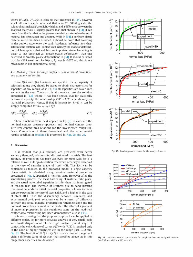
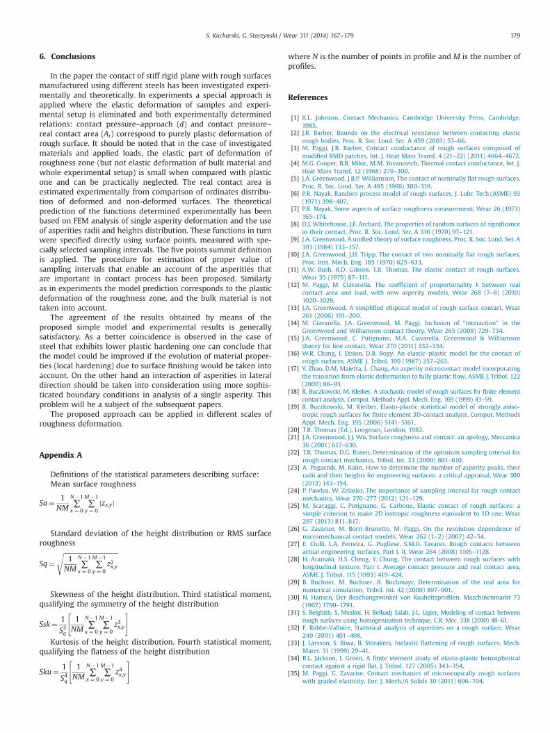
These functions were next applied in Eq. (3) to calculate thenominal contact pressure–approach and nominal contact pres-sure–real contact area relations for the investigated rough sur-faces. Comparison of these theoretical and the experimentalresults specified in Section 3 is presented in Figs. 25 and 26.

5. Discussion

It is evident that p–d relations are predicted with betteraccuracy than p–Ar relations for all considered materials. The bestaccuracy of prediction has been achieved for steel s235 for p–drelation as well as for p–Ar relation. The worst accuracy is observedin the case of samples made of steel 40H. This fact can beexplained as follows. In the proposed model a single asperitycharacteristic is calculated using nominal material propertiespresented in Fig. 1, specified in tension tests. However after thesandblasting process the local hardening of material take place,and the actual material of asperities is stiffer than that investigatedin tension test. The increase of stiffness due to sand blastingtreatment depends on initial material properties; a lower increasecan be expected in the case of steel s235, and a higher in the caseof steel 40H. Thus the discrepancy between simulated andexperimental p–d, p–Ar relations can be a result of differencebetween the actual material properties in roughness zone and thenominal properties assumed in the model. The effect of a gradientof material properties in the roughness zone on the load–realcontact area relationship has been demonstrated also in [35].

It is worth noting that the proposed approach can be applied indifferent scales, i.e. for more accurate analysis of very small loadsand small displacement of the rigid surface (initial stage ofcontact) the coincidence of curves N(Z) with Ng(Z) is required onlyin the zone of higher roughness e.g. in the range 0.01–0.02 mm,Fig. 21. The best fit of N(Z) to Ng(Z) in such a limited range willyield a different value of dx than that specified above, as in thisrange finer asperities are deformed.

02468

1012

0 500 1000normal load [MPa]

disp

lace

men

t [m

m x

10-3

]

02468

101214

0 200 400 600normal load [MPa]

disp

lace

men

t [m

m x1

0-3]

02468

101214

0 200 400 600normal load [MPa]

disp

lace

men

t [m

m x1

0-3]

steel 45

experiments

steel 235

experiment

model

model

steel H40

experiment

model

steel 40H

experiment

model

steel H40

experiment

Fig. 25. Load–approach curves for the analyzed steels.

05

10152025303540

0 200 400 600 800nominal pressure [MPa]

A r

[%]

40H exp. S235 exp.h40 modelS235 model

05

101520253035

0 200 400 600 800nominal pressure [Mpa]

A r

[%]

45 exp.S45 model

Fig. 26. Load–real contact area curves for rough surfaces on analyzed samples:(a) s235 and 40H and (b) steel 45.

S. Kucharski, G. Starzynski / Wear 311 (2014) 167–179178

6. Conclusions

In the paper the contact of stiff rigid plane with rough surfacesmanufactured using different steels has been investigated experi-mentally and theoretically. In experiments a special approach isapplied where the elastic deformation of samples and experi-mental setup is eliminated and both experimentally determinedrelations: contact pressure–approach (d) and contact pressure–real contact area (Ar) correspond to purely plastic deformation ofrough surface. It should be noted that in the case of investigatedmaterials and applied loads, the elastic part of deformation ofroughness zone (but not elastic deformation of bulk material andwhole experimental setup) is small when compared with plasticone and can be practically neglected. The real contact area isestimated experimentally from comparison of ordinates distribu-tion of deformed and non-deformed surfaces. The theoreticalprediction of the functions determined experimentally has beenbased on FEM analysis of single asperity deformation and the useof asperities radii and heights distribution. These functions in turnwere specified directly using surface points, measured with spe-cially selected sampling intervals. The five points summit definitionis applied. The procedure for estimation of proper value ofsampling intervals that enable an account of the asperities thatare important in contact process has been proposed. Similarlyas in experiments the model prediction corresponds to the plasticdeformation of the roughness zone, and the bulk material is nottaken into account.

The agreement of the results obtained by means of theproposed simple model and experimental results is generallysatisfactory. As a better coincidence is observed in the case ofsteel that exhibits lower plastic hardening one can conclude thatthe model could be improved if the evolution of material proper-ties (local hardening) due to surface finishing would be taken intoaccount. On the other hand an interaction of asperities in lateraldirection should be taken into consideration using more sophis-ticated boundary conditions in analysis of a single asperity. Thisproblem will be a subject of the subsequent papers.

The proposed approach can be applied in different scales ofroughness deformation.

Appendix A

Definitions of the statistical parameters describing surface:Mean surface roughness

Sa¼ 1NM

∑N�1

x ¼ 0∑

M�1

y ¼ 0jzx;yj

Standard deviation of the height distribution or RMS surfaceroughness

Sq¼ffiffiffiffiffiffiffiffiffiffiffiffiffiffiffiffiffiffiffiffiffiffiffiffiffiffiffiffiffiffiffiffiffiffi1

NM∑

N�1

x ¼ 0∑

M�1

y ¼ 0z2x;y

s

Skewness of the height distribution. Third statistical moment,qualifying the symmetry of the height distribution

Ssk¼ 1

S3q

1NM

∑N�1

x ¼ 0∑

M�1

y ¼ 0z3x;y

" #

Kurtosis of the height distribution. Fourth statistical moment,qualifying the flatness of the height distribution

Sku¼ 1

S4q

1NM

∑N�1

x ¼ 0∑

M�1

y ¼ 0z4x;y

" #

where N is the number of points in profile and M is the number ofprofiles.

References

[1] K.L. Johnson, Contact Mechanics, Cambridge University Press, Cambridge,1985.

[2] J.R. Barber, Bounds on the electrical resistance between contacting elasticrough bodies, Proc. R. Soc. Lond. Ser. A 459 (2003) 53–66.

[3] M. Paggi, J.R. Barber, Contact conductance of rough surfaces composed ofmodified RMD patches, Int. J. Heat Mass Transf. 4 (21–22) (2011) 4664–4672.

[4] M.G. Cooper, B.B. Mikic, M.M. Yovanovich, Thermal contact conductance, Int. J.Heat Mass Transf. 12 (1968) 279–300.

[5] J.A. Greenwood, J.B.P. Williamson, The contact of nominally flat rough surfaces,Proc. R. Soc. Lond. Ser. A 495 (1966) 300–319.

[6] P.R. Nayak, Random process model of rough surfaces, J. Lubr. Tech.(ASME) 93(1971) 398–407.

[7] P.R. Nayak, Some aspects of surface roughness measurement, Wear 26 (1973)165–174.

[8] D.J. Whitehouse, J.F. Archard, The properties of random surfaces of significancein their contact, Proc. R. Soc. Lond. Ser. A 316 (1970) 97–121.

[9] J.A. Greenwood, A unified theory of surface roughness, Proc. R. Soc. Lond. Ser. A393 (1984) 133–157.

[10] J.A. Greenwood, J.H. Tripp, The contact of two nominally flat rough surfaces,Proc. Inst. Mech. Eng. 185 (1970) 625–633.

[11] A.W. Bush, R.D. Gibson, T.R. Thomas, The elastic contact of rough surfaces,Wear 35 (1975) 87–111.

[12] M. Paggi, M. Ciavarella, The coefficient of proportionality k between realcontact area and load, with new asperity models, Wear 268 (7–8) (2010)1020–1029.

[13] J.A. Greenwood, A simplified elliptical model of rough surface contact, Wear261 (2006) 191–200.

[14] M. Ciavarella, J.A. Greenwood, M. Paggi, Inclusion of “interaction” in theGreenwood and Williamson contact theory, Wear 265 (2008) 729–734.

[15] J.A. Greenwood, C. Putignano, M.A. Ciavarella, Greenwood & Williamsontheory for line contact, Wear 270 (2011) 332–334.

[16] W.R. Chang, I. Etsion, D.B. Bogy, An elastic–plastic model for the contact ofrough surfaces, ASME J. Tribol. 109 (1987) 257–263.

[17] Y. Zhao, D.M. Maietta, L. Chang, An asperity microcontact model incorporatingthe transition from elastic deformation to fully plastic flow, ASME J. Tribol. 122(2000) 86–93.

[18] R. Buczkowski, M. Kleiber, A stochastic model of rough surfaces for finite elementcontact analysis, Comput. Methods Appl. Mech. Eng. 169 (1999) 43–59.

[19] R. Buczkowski, M. Kleiber, Elasto-plastic statistical model of strongly aniso-tropic rough surfaces for finite element 3D-contact analysis, Comput. MethodsAppl. Mech. Eng. 195 (2006) 5141–5161.

[20] T.R. Thomas (Ed.), Longman, London, 1982.[21] J.A. Greenwood, J.J. Wu, Surface roughness and contact: an apology, Meccanica

36 (2001) 617–630.[22] T.R. Thomas, D.G. Rosen, Determination of the optimum sampling interval for

rough contact mechanics, Tribol. Int. 33 (2000) 601–610.[23] A. Pogacnik, M. Kalin, How to determine the number of asperity peaks, their

radii and their heights for engineering surfaces: a critical appraisal, Wear 300(2013) 143–154.

[24] P. Pawlus, W. Zelasko, The importance of sampling interval for rough contactmechanics, Wear 276–277 (2012) 121–129.

[25] M. Scaraggi, C. Putignano, G. Carbone, Elastic contact of rough surfaces: asimple criterion to make 2D isotropic roughness equivalent to 1D one, Wear297 (2013) 811–817.

[26] G. Zavarise, M. Borri-Brunetto, M. Paggi, On the resolution dependence ofmicromechanical contact models, Wear 262 (1–2) (2007) 42–54.

[27] E. Ciulli, L.A. Ferreira, G. Pugliese, S.M.O. Tavares, Rough contacts betweenactual engineering surfaces. Part I, II, Wear 264 (2008) 1105–1128.

[28] H. Aramaki, H.S. Cheng, Y. Chung, The contact between rough surfaces withlongitudinal texture. Part I. Average contact pressure and real contact area,ASME J. Tribol. 115 (1993) 419–424.

[29] B. Buchner, M. Buchner, B. Buchmayr, Determination of the real area fornumerical simulation, Tribol. Int. 42 (2009) 897–901.

[30] N. Hansen, Der Boschungswinkel von Rauheitsprofilen, Maschinenmarkt 73(1967) 1790–1791.

[31] S. Belghith, S. Mezlini, H. Belhadj Salah, J-L. Ligier, Modeling of contact betweenrough surfaces using homogenization technique, C.R. Mec. 338 (2010) 48–61.

[32] F. Robbe-Valloire, Statistical analysis of asperities on a rough surface, Wear249 (2001) 401–408.

[33] J. Larsson, S. Biwa, B. Storakers, Inelastic flattening of rough surfaces, Mech.Mater. 31 (1999) 29–41.

[34] R.L. Jackson, I. Green, A finite element study of elasto-plastic hemisphericalcontact against a rigid flat, J. Tribol. 127 (2005) 343–354.

[35] M. Paggi, G. Zavarise, Contact mechanics of microscopically rough surfaceswith graded elasticity, Eur. J. Mech./A Solids 30 (2011) 696–704.

S. Kucharski, G. Starzynski / Wear 311 (2014) 167–179 179