study of differential gps system for uavs en enginyeria de vehicles aeroespacials treball de fi de...
TRANSCRIPT
Grau en Enginyeria de Vehicles Aeroespacials
Treball de fi de grau
Study of differential GPS
system for UAVs
Document content : REPORT
Delivery date: 22/06/2016
Author: Oriol Trujillo Martí
Director: Antoni Barlabé Dalmau
Codirector: Manuel Soria Guerrero


Acknowledgements
I would like to express all my gratitude to all the people that have contributed or helped
somehow to the development of this study.
First, I want to thank Professor Antoni Barlabé for his guidance, technical support and
encouragement in carrying out this project.
My family and friends for pulling me up, and especially to my dear friend David and lovely
sister Mireia, for sacrificing their valuable time for science and be there in the critical
moments.
To all of them, thank you.
ii Oriol Trujillo
Martí
Contents
List of Figures iv
List of Tables vii
1. Aim 1
2. Scope 2
3. Requirements 3
4. Justification 4
5. State of the art 5
6. Proposed procedure 6
6.1 Approach, issues and solutions . . . . . . . . . . . . . . . . . . . . . . . . . . . . . . . . . 6
6.2 Development of the project . . . . . . . . . . . . . . . . . . . . . . . . . . . . . . . . . . . . . 8
6.2.1 Implemented DGPS methodologies . . . . . . . . . . . . . . . . . . . . . . . . 9
6.2.2 Overall view of the procedure . . . . . . . . . . . . . . . . . . . . . . . . . . . . 28
7. Hardware and connections 31
7.1 GPS receivers . . . . . . . . . . . . . . . . . . . . . . . . . . . . . . . . . . . . . . . . . . . . . . 31
7.2 Connections Schematics . . . . . . . . . . . . . . . . . . . . . . . . . . . . . . . . . . . . . . 34
7.2.1 Rover . . . . . . . . . . . . . . . . . . . . . . . . . . . . . . . . . . . . . . . . . . . . . . . 36
7.2.2 Base Station . . . . . . . . . . . . . . . . . . . . . . . . . . . . . . . . . . . . . . . . . . 37
8. Software 39
8.1 Mission Planner . . . . . . . . . . . . . . . . . . . . . . . . . . . . . . . . . . . . . . . . . . . . 39
8.2 U-Center . . . . . . . . . . . . . . . . . . . . . . . . . . . . . . . . . . . . . . . . . . . . . . . . . . 39
8.2.1 Messages and Protocols . . . . . . . . . . . . . . . . . . . . . . . . . . . . . . . . 40
8.2.2 Decoded messages . . . . . . . . . . . . . . . . . . . . . . . . . . . . . . . . . . . . 42
8.3 Sublime Text . . . . . . . . . . . . . . . . . . . . . . . . . . . . . . . . . . . . . . . . . . . . . . . 43
8.4 Implemented MATLAB Code . . . . . . . . . . . . . . . . . . . . . . . . . . . . . . . . . . . 44
8.4.1 Flowcharts. . . . . . . . . . . . . . . . . . . . . . . . . . . . . . . . . . . . . . . . . . . . 44
8.5 Google Earth . . . . . . . . . . . . . . . . . . . . . . . . . . . . . . . . . . . . . . . . . . . . . . . 58
9. Results 59

iii Oriol Trujillo
Martí
9.1 Test design . . . . . . . . . . . . . . . . . . . . . . . . . . . . . . . . . . . . . . . . . . . . . . . . 59
9.1.1 Selection of Location . . . . . . . . . . . . . . . . . . . . . . . . . . . . . . . . . . . 59
9.1.2 Length . . . . . . . . . . . . . . . . . . . . . . . . . . . . . . . . . . . . . . . . . . . . . . . 60
9.1.3 Message configuration . . . . . . . . . . . . . . . . . . . . . . . . . . . . . . . . . . 61
9.2 Tests . . . . . . . . . . . . . . . . . . . . . . . . . . . . . . . . . . . . . . . . . . . . . . . . . . . . 62
9.2.1 Test 1: static at reference location . . . . . . . . . . . . . . . . . . . . . . . . . 62
9.2.2 Test 2: static at different locations . . . . . . . . . . . . . . . . . . . . . . . . . 71
10. Environmental Impact 75
11. Future planning and scheduling 76
11.1 Proposed schedule for future work . . . . . . . . . . . . . . . . . . . . . . . . . . . . . . 77
12. Conclusions 78
13. Bibliography 80

iv Oriol Trujillo
Martí
List of Figures
1. Navigation solution correction concept . . . . . . . . . . . . . . . . . . . . . . . . . . . . . . 13
2. Virtual Space Vehicles distribution (36 satellites, 1km of radius). . . . . . . . . . . 14
3. Least squares method example . . . . . . . . . . . . . . . . . . . . . . . . . . . . . . . . . . . . 17
4. Navigation message frames, image from [4] . . . . . . . . . . . . . . . . . . . . . . . . . . 19
5. Telemetry word structure. Image from [15] . . . . . . . . . . . . . . . . . . . . . . . . . . . 20
6. Hand-over word, image from [15] . . . . . . . . . . . . . . . . . . . . . . . . . . . . . . . . . . 20
7. GPS time, Z-count and truncated Z-coount, image from [4] . . . . . . . . . . . . . . 21
8. Navigation Message Subframe 1 structure, image from [15] . . . . . . . . . . . . . 21
9. Navigation Message Subframe 2, image from [15] . . . . . . . . . . . . . . . . . . . . . 22
10. Navigation Message Subframe 3, image from [15] . . . . . . . . . . . . . . . . . . . . . 22
11. Visible healthy satellites' paths tracked along test 1, approximately 10 min . . 26
12. Range Residual, pseudorange and geometric range relationship . . . . . . . . . . 27
13. Overall scheme of the procedure . . . . . . . . . . . . . . . . . . . . . . . . . . . . . . . . . . . 29
14. Available GPS receiver, own image and edited picture from https://3drobotics.zendesk.com/hc/en-us . . . . . . . . . . . . . . . . . . . . . . . . . . . . . 34
15. Possible configurations of the hardware components . . . . . . . . . . . . . . . . . . . 35
16. Pixhawk, micro USB and DF13 cables, images from https://pixhawk.org, http://mikrokopter.altigator.com/ and http://reciclatecnologia.com/. . . . . . . . . . 36
17. USB to TTL-232R serial cable to DF13 joint . . . . . . . . . . . . . . . . . . . . . . . . . . 37
18. NMEA Protocol frame, as specified in [17] . . . . . . . . . . . . . . . . . . . . . . . . . . . 41
19. UBX frame structure, defined in [17] . . . . . . . . . . . . . . . . . . . . . . . . . . . . . . . . 41
20. Sublime text screenshot showing the firsts 13 lines (of 77756) of binary data file about to be exported . . . . . . . . . . . . . . . . . . . . . . . . . . . . . . . . . . . . . 43
21. Flowchart of DGPS.m . . . . . . . . . . . . . . . . . . . . . . . . . . . . . . . . . . . . . . . . . . . 45
v Oriol Trujillo
Martí
22. Flowchart of messageDecoder.m . . . . . . . . . . . . . . . . . . . . . . . . . . . . . . . . . . 46
23. NMEA decoder, attachment to flowchart of messageDecoder.m . . . . . . . . . . 47
24. Flowchart of getGNSSparameters.m . . . . . . . . . . . . . . . . . . . . . . . . . . . . . . . . 48
25. Time assignment and sending attachment to flowchart of getGNSSparameters.m . . . . . . . . . . . . . . . . . . . . . . . . . . . . . . . . . . . . . . . . . . 49
26. Flowchart of trackSV.m . . . . . . . . . . . . . . . . . . . . . . . . . . . . . . . . . . . . . . . . . . 50
27. Flowchart of time coordination . . . . . . . . . . . . . . . . . . . . . . . . . . . . . . . . . . . . . 51
28. Flowchart of computeCorrectionsOFFSET.m . . . . . . . . . . . . . . . . . . . . . . . . . 52
29. Flowchart of computeCorrectionsCOMMON.m . . . . . . . . . . . . . . . . . . . . . . . . 53
30. Flowchart of computeCorrectionsReal.m . . . . . . . . . . . . . . . . . . . . . . . . . . . . . 54
31. Flowchart of computeCorrectionsVirtual.m . . . . . . . . . . . . . . . . . . . . . . . . . . . 55
32. Flowchart of computePosition.m . . . . . . . . . . . . . . . . . . . . . . . . . . . . . . . . . . . 56
33. Flowchart of leastSquaresPos.m . . . . . . . . . . . . . . . . . . . . . . . . . . . . . . . . . . . 57
34. Aerial view of Avinguda de l'Onze de Setembre, Sant Joan Despí. Image taken from Google Earth . . . . . . . . . . . . . . . . . . . . . . . . . . . . . . . . . . . . 60
35. Test 1. Distance from each solution to reference location . . . . . . . . . . . . . . . . 62
36. Test 1. OFFSET corrected path vs. uncorrected path, horizontal path and 3D path plotted on Google Earth . . . . . . . . . . . . . . . . . . . . . . . . . . . . . . . . . . . 63
37. Test 1. NavSol - Real SVs corrected path vs. uncorrected path, horizontal path and 3D path plotted on Google Earth . . . . . . . . . . . . . . . . . . . . . . . . . . . 64
38. Test 1. NavSol - Virtual SVs corrected path vs. uncorrected path, horizontal path and 3D path plotted on Google Earth . . . . . . . . . . . . . . . . . . . . . . . . . . . 65
39. Test 1. COMMON corrected path vs. uncorrected path, horizontal path and 3D path plotted on Google Earth . . . . . . . . . . . . . . . . . . . . . . . . . . . . . . . . . . . 66
40. Test 1. Base Station uncorrected path vs. Rover uncorrected path, horizontal path and 3D path plotted on Google Earth . . . . . . . . . . . . . . . . . . . 67
41. Test 1. Distance between uncorrected rover and base station paths . . . . . . . 68
42. GPS sources of error . . . . . . . . . . . . . . . . . . . . . . . . . . . . . . . . . . . . . . . . . . . . ¡Error! Marcador no definido.
43. Test 1. Absolutely uncorrected measurements solutin vs. rover final solution 70
44. Test 1. Position DIlution of Precision (PDOP) comparison . . . . . . . . . . . . . . . 70
45. Test 2 receivers' locations . . . . . . . . . . . . . . . . . . . . . . . . . . . . . . . . . . . . . . . . 71

vi Oriol Trujillo
Martí
46. Test 2. Distance from each solution to rover's known location . . . . . . . . . . . . 72
47. Test 1. Distance to each solution to reference location . . . . . . . . . . . . . . . . . . 72
48. Test 2. OFFSET corrected path vs. uncorrected path, horizontal path and 3D path plotted on Google Earth . . . . . . . . . . . . . . . . . . . . . . . . . . . . . . . . . . . 73
49. Test 2. NavSol - Virtual SVs corrected path vs. uncorrected path, horizontal path and 3D path plotted on Google Earth . . . . . . . . . . . . . . . . . . . 73
vii Oriol Trujillo
Martí
List of Tables
1. GPS sources of error . . . . . . . . . . . . . . . . . . . . . . . . . . . . . . . . . . . . . . . . . . . . . 6
2. Main features of the employed DGPS correction method . . . . . . . . . . . . . . . . . 8
3. Variables lengend - Least squares method definition . . . . . . . . . . . . . . . . . . . 15
4. Subframe 2 and 3. Definition of parameters, according to [15] . . . . . . . . . . . . 23
5. Computation of a satellite's ECEF position from ephemeris parameters, as is defined in [15] . . . . . . . . . . . . . . . . . . . . . . . . . . . . . . . . . . . . . . . . . . . . . . . . 25
6. Main features of U-Blox NEO-7N module, more information can be found in [7] . . . . . . . . . . . . . . . . . . . . . . . . . . . . . . . . . . . . . . . . . . . . . . . . . . . . . . . . . 32
7. Main features of the Taoglas GPS patch 1575 MHz antenna, information obtained from [18] . . . . . . . . . . . . . . . . . . . . . . . . . . . . . . . . . . . . . . . . . . . . . . 33
8. Features and specifications of 3DR U-Blox GPS with compass kit, according to [6] . . . . . . . . . . . . . . . . . . . . . . . . . . . . . . . . . . . . . . . . . . . . . . . . 33
9. TTL-232R and DF13 joint colour code . . . . . . . . . . . . . . . . . . . . . . . . . . . . . . . 37
10. Decoded messages description . . . . . . . . . . . . . . . . . . . . . . . . . . . . . . . . . . . . 42
11. Require messages for each correction mode . . . . . . . . . . . . . . . . . . . . . . . . . 61
12. Test 1. NavSol - Virtual SVs distribution description . . . . . . . . . . . . . . . . . . . . 65

1 Oriol Trujillo
Martí
1. Aim
The aim of the project is to track an Unmanned Aerial Vehicle (UAV) with a centimetre-
level accuracy by implementing a Differential Global Positioning System (DGPS) using
a pair of low-cost Global Positioning System (GPS) receivers. DGPS corrections will be
applied a posteriori and, if the results are satisfactory, it will be studied the possibility to
implement real-time DGPS corrections.
2 Oriol Trujillo
Martí
2. Scope
This project involves understanding GPS principles and performance, as well as its
sources of error, so an initial learning phase is required. Once the bases are acquired,
the stages of the procedure must be defined.
The first step is to communicate with the GPS receivers, so the connections and interface
must be specified. Achieved that, receivers have to be set and input data stored and
exported into a convenient format to be treated afterward. To do that it is necessary to
get familiarized with the work’s environment and begin to understand the basics of GPS
protocols, as well as the receiver’s configuration settings.
At this point, it has been revealed that available GPS receivers do not output raw data,
so solution must be found to overcome this problem.
The next stage is to begin the program that will perform all the correction tasks. Which
first purpose, must be to read GPS stored data, decode it and extract the information
contained inside. Each useful binary message’s structure must be known, so a deeper
knowledge of UBX and NMEA GPS’ protocols is obligate.
Once information is extracted, it must be processed and corrections applied.
All the implemented code must validated and then tested, this will imply some field work.
Finally, results have to be analysed, and if they are satisfactory, the methodology can be
implemented for real-time applications.
The optional tasks would include obtaining a communicating system, in order to receive
data and transmit corrections in real time. Additionally, it is possible that the original
program should be adapted to make it optimal, allowing fast corrections.

3 Oriol Trujillo
Martí
3. Requirements
The requirements that this project must fulfil to be considered successfully are:
A. Obtain a centimetre-level accuracy positioning.
B. Low cost of the whole system.
As an optional requirement:
C. The whole system has to be fast enough to be applied in real-time.
4 Oriol Trujillo
Martí
4. Justification
The use of Drones or Unmanned Aerial Vehicles in civil applications has grown
exponentially in the last years and it currently does. They help society performing tasks
that have to be done in the air, at some altitude or that involve flight somehow. Until few
years ago, many of these would have been very expensive or impossible. In many of
these applications a higher positioning precision than a conventional GPS can offer is
required.
In order to improve positioning precision, augmentation systems, such as Differential
GPS, are used.
DGPS is not a new concept and it has been used in aviation, coastguard services, marine
transport, and so forth, for more than two decades. However, this equipment is complex,
expensive and covers large areas. What this project seeks is a low-cost technique based
on DGPS that achieves high precision positioning in small ranges in order to satisfy this
new demanding.
5 Oriol Trujillo
Martí
5. State of the art
Currently, a basic single-frequency GPS receiver can be purchased by approximately
50€ with around 3m of horizontal precision thanks to EGNOS, the Satellite-Based
Augmentation System (SBAS) that covers Europe. In those countries where any SBAS
service is provided, the horizontal error for standard precision is around 10m, according
to [11].
Dual-frequency receivers can achieve centimetre-level accuracy for several thousands
of euros.
Another way to improve positioning without expending such quantities of money, is using
Differential GPS corrections. DGPS corrections can be performed running the open-
source software RTK solutions, but with a great computational cost complicating real-
time applications or RTKLIB, which supports real-time and post-processing corrections
reaching until decimetre-level accuracy by a high computational cost. However, RTKLIB
does not support many receivers such as the U-Blox NEO family since they do not
provide raw data [13]. This is an important lack since these receivers are very common,
for instance are the receivers that 3D Robotics uses. Raw capable receivers can be
obtained by around 70€.
Other alternatives are like SwiftNav ‘Piksi’ GPS that can cost around 450€ each receiver
and provide centimetre-level accuracies or applications based on RINEX (Receiver
Independent Exchange Format), as can be found in [12].
The utility of this project is to supply DGPS corrections to the wide group of unsupported
receivers such as the available for the implementation of this project.
6 Oriol Trujillo
Martí
6. Proposed procedure
In the following sections, it has been assumed a basic understanding of GPS principles,
its sources of error and augmentations such as DGPS. Only the most indispensable
aspects are pointed out below. For the interested reader, a more detailed explanation is
attached in annex A.
6.1 Approach, issues and solutions
In this project is demanded a low-cost enhancement system based on DGPS that
improves basic GPS precision. Recall that, a minimum of 2 receivers with at least one of
them at known location, base station/s and rover respectively, are required to apply
DGPS corrections. Using this technique we are able to cancel common errors, between
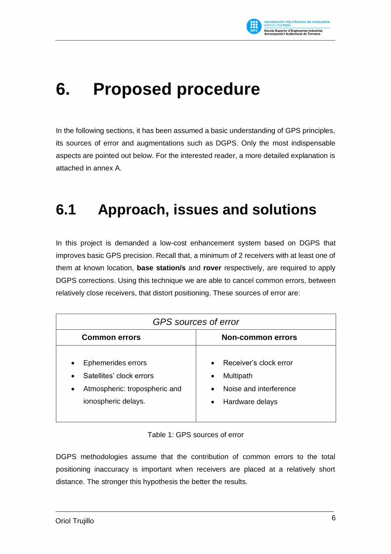
relatively close receivers, that distort positioning. These sources of error are:
GPS sources of error
Common errors Non-common errors
Ephemerides errors
Satellites’ clock errors
Atmospheric: tropospheric and
ionospheric delays.
Receiver’s clock error
Multipath
Noise and interference
Hardware delays
Table 1: GPS sources of error
DGPS methodologies assume that the contribution of common errors to the total
positioning inaccuracy is important when receivers are placed at a relatively short
distance. The stronger this hypothesis the better the results.
7 Oriol Trujillo
Martí
Corrections can be applied in the pseudorange domain or in the position domain. The
first just needs to know the positioning solution and the latter also demands satellites’
positions and pseudoranges.
However, the available components for the development of this project are 2 single-
frequency receivers incapable to provide raw data (restricted by the manufacturer).
So, it is not possible to get receivers’ pseudorange measurements, which are compulsory
for pseudorange domain Differential GPS corrections.
At this point, a decisive controversy is presented. The proposals to overcome this affair
are:
Obtain raw data even it is not officially supported. Measuring pseudoranges is
the main feature of GPS receivers and they are used to compute positioning, so
these values are contained in the module. There is one configuration message
that allows the receiver to output raw data, but it is unknown. It has been found
several codes on some forums but for similar receivers (the previous generation
of the available devices), and suggestions referred to the used ones, all have
been attempted once it has been possible to communicate with the receivers and
all failed.
Indirectly estimate raw data. Pseudorange measurements can be estimated
reversing navigation solution’s computation process, if navigation solution,
satellites’ positions and a key parameter called Range Residuals (RR) are
known.
Buy a pair of raw capable receivers. This is the last option, since it implies extra
costs and time. It will only be considered if none of the above is feasible.
It has been chosen the second alternative, since it uses the available resources, most
of them granted by the Aerospace Department of ESEIAAT (Escola Tècnica Superior
d’Enginyeries Industrial, Aeroespacial I Audiovisual de Terrassa), and allows to perform
DGPS corrections to the all models even if they are not raw capable, supplying this way,
a feasible enhancement service that can serve the school purposes.
8 Oriol Trujillo
Martí
6.2 Development of the project
In this section it is presented the procedure that is followed to accomplish the goals,
introducing the tasks that must be executed by hardware components and software, and
finally illustrating how all of them are integrated to attain a greater purpose.
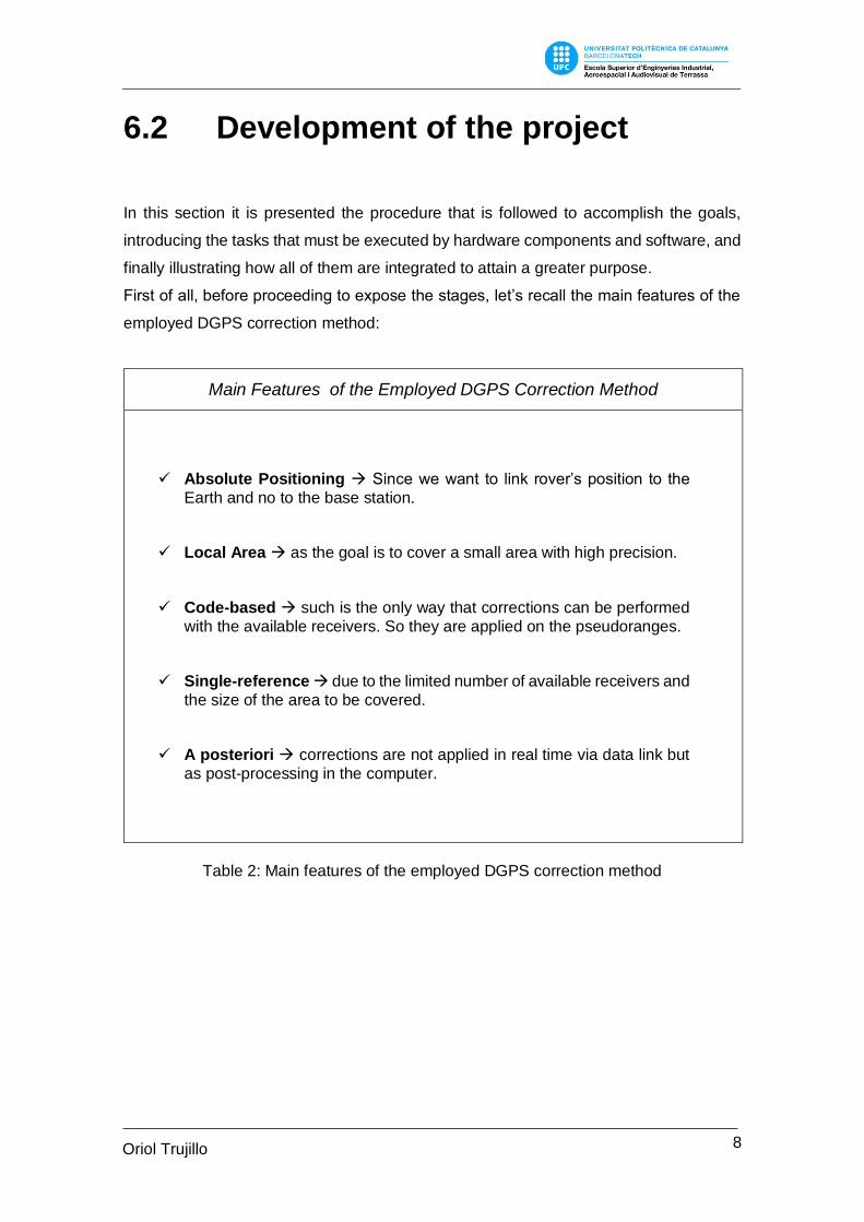
First of all, before proceeding to expose the stages, let’s recall the main features of the
employed DGPS correction method:
Main Features of the Employed DGPS Correction Method
Absolute Positioning Since we want to link rover’s position to the
Earth and no to the base station.
Local Area as the goal is to cover a small area with high precision.
Code-based such is the only way that corrections can be performed
with the available receivers. So they are applied on the pseudoranges.
Single-reference due to the limited number of available receivers and
the size of the area to be covered.
A posteriori corrections are not applied in real time via data link but
as post-processing in the computer.
Table 2: Main features of the employed DGPS correction method

9 Oriol Trujillo
Martí
6.2.1 Implemented DGPS methodologies
Four correction methodologies have been considered to achieve the goal of this project:
one in the position domain (treats the error as offset) and three in the pseudorange
domain. These are, classical or common DGPS corrections and a proposal of this
study presented as two variants of the same idea. These methodologies are based on
navigation solution’s correction, and have been called Navigation Solution– Real SVs
and Navigation Solution – Virtual SVs, respectively.
6.2.1.1 Position domain correction
Position domain correction is the simplest one. It does not require any knowledge about
Space Vehicles (SV) position neither pseudoranges, only rover position and base
station measured and known position.
Position domain correction consists on the addition of an offset applied directly on the
final navigation solution, which is basically the difference between the true location of the
base station and the base station navigation solution. This can be written as:
∆𝑟(𝑡) = 𝑟𝑡𝑟𝑢𝑒 − 𝑟(𝑡)𝐵𝑆 (6.1)
𝑟(𝑡)𝑅𝑐𝑜𝑟𝑟 = 𝑟(𝑡)𝑅𝑢𝑛𝑐 + ∆𝑟(𝑡) (6.2)
Where 𝑟 stands for the position vector and the subscripts true, BS, Rcorr, Runc mean
true locations, base station, rover corrected and rover uncorrected respectively.
This technique is extremely simple, but several aspects have to be taken into account
before applying it. Has to be ensured that both receivers, rover and base station, use
the same set of satellites to make pseudoranges measurements all the time. Also, the
same solution technique (least squares, Kalman filter, WLS, etc.), with the same
parameters (filter tunings, smoothing time constants, etc.), must be warranted.
These conditions make of this, an impracticable real-time method, but can be performed
as a post-processing correction.
This methodology assumes that base station and rover final solution errors are similar
values. A reading of this, is that the method corrects the error introduced by the
atmosphere over the final solution, which seems reasonable, but also errors due to
10 Oriol Trujillo
Martí
receivers’ hardware, noise and interference, and multipath (which is expected to be low
but in those cases that it is not, makes the method inapplicable). The latter set of errors
is independent from one receiver to another, so the lower weight of these errors the
better the performance.
Note that, as the correction is applied over the final solutions, receiver and satellite clock
corrections are already done. The same way tropospheric and ionospheric delays are
attempted to be corrected by the receivers using models and correction parameters, this
method fixes models’ limitations.
6.2.1.2 Pseudorange domain corrections
Pseudorange domain corrections differ from the latter on where the corrections are
applied. Instead of correcting the final solution, corrections are computed and applied
over each pseudorange. That are also expected to be similar if receivers are relatively
close.
Once pseudoranges have been corrected, the corrected solution is found by normal
triangulation. In this project it has been used the least squares method, presented in
section 6.2.1.2.4.
Finally, with the intention of having a measure of the confidence in results, dilution of
precision is computed such is defined in section 6.2.1.2.5 or explained in the annex
section A.1.2.
The essential parameters for computing pseudprange measurements are:
Rover position
Base station position
Base station true location
Space Vehicles’ positions computed from ephemerides.
Pseudoranges Available GPS receivers do not output pseudoranges, they
must be estimated.
Sections 6.2.1.3 and 6.2.1.4 explain how satellites’ positions and pseudoranges are
computed.
11 Oriol Trujillo
Martí
6.2.1.2.1 Common DGPS correction
The common or classic method compares the pseudorange measurement with the real
range between the base station m, in the known position, to the satellite k. The difference,
which is the error, is composed by the base station receiver clock delay, ionospheric and
tropospheric errors plus a residual error. The correction is applied to the rover receiver i,
expecting common ionospheric and tropospheric delays.
Let be Pmk the measured pseudorange, ρm
k the geometric range, dtm the base station
clock offset, Imk the total ionospheric error from satellite k to the receiver m, Tmk the
tropospheric error and emk the residual error that the least squares method tries to
minimize.
𝑃𝑚𝑘 = 𝜌𝑚
𝑘 + 𝑐𝑑𝑡𝑚 + 𝐼𝑚𝑘 + 𝑇𝑚
𝑘+𝑒𝑚𝑘 (6.3)
The differential correction is:
∆𝑃𝑚𝑘 = 𝜌𝑚
𝑘 − 𝑃𝑚𝑘 = −𝑐𝑑𝑡𝑚 − 𝐼𝑚
𝑘 − 𝑇𝑚𝑘−𝑒𝑚
𝑘 (6.4)
The same way, the measured pseudorange between satellite k and the rover receiver i,
can be written as:
𝑃𝑖𝑘 = 𝜌𝑖
𝑘 + 𝑐𝑑𝑡𝑖 + 𝐼𝑖𝑘 + 𝑇𝑖
𝑘+𝑒𝑖𝑘 (6.5)
Under the hypothesis 𝐼𝑚𝑘 + 𝑇𝑚
𝑘 ≈ 𝐼𝑖𝑘 + 𝑇𝑖
𝑘 , the pseudorange correction is applied to the
rover GPS receiver pseudorange measurement:
𝑃𝑖,𝑐𝑜𝑟𝑟𝑘 = 𝑃𝑖
𝑘 + ∆𝑃𝑚𝑘 = 𝜌𝑖
𝑘 + 𝑐(𝑑𝑡𝑖 − 𝑑𝑡𝑚)+𝑒𝑖𝑘 + (𝐼𝑖
𝑘 − 𝐼𝑚𝑘 ) + (𝑇𝑖
𝑘 − 𝑇𝑚𝑘 ) − 𝑒𝑚
𝑘 (6.6)
Note that if the latter hypothesis is acceptable and once dti-dtk is computed, the
measured pseudorange will only differ from the real geometric range a distance of value
eik-em
k.
12 Oriol Trujillo
Martí
6.2.1.2.2 Navigation Solution correction – Real SVs
In this project it is proposed an alternative correction method to the classical one. As the
goal of the project is to implement post-processing DGPS correction, it has been
suggested taking advantage of this fact and compute corrections over the final navigation
solution instead on pseudorange measurements.
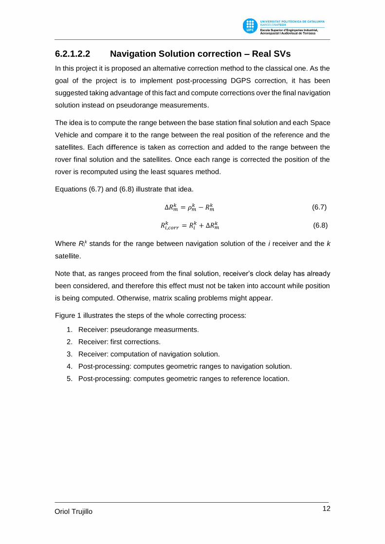
The idea is to compute the range between the base station final solution and each Space
Vehicle and compare it to the range between the real position of the reference and the
satellites. Each difference is taken as correction and added to the range between the
rover final solution and the satellites. Once each range is corrected the position of the
rover is recomputed using the least squares method.
Equations (6.7) and (6.8) illustrate that idea.
∆𝑅𝑚𝑘 = 𝜌𝑚
𝑘 − 𝑅𝑚𝑘 (6.7)
𝑅𝑖,𝑐𝑜𝑟𝑟𝑘 = 𝑅𝑖
𝑘 + ∆𝑅𝑚𝑘 (6.8)
Where Rik stands for the range between navigation solution of the i receiver and the k
satellite.
Note that, as ranges proceed from the final solution, receiver’s clock delay has already
been considered, and therefore this effect must not be taken into account while position
is being computed. Otherwise, matrix scaling problems might appear.
Figure 1 illustrates the steps of the whole correcting process:
1. Receiver: pseudorange measurments.
2. Receiver: first corrections.
3. Receiver: computation of navigation solution.
4. Post-processing: computes geometric ranges to navigation solution.
5. Post-processing: computes geometric ranges to reference location.
13 Oriol Trujillo
Martí
6. Post-processing: computes the difference.
Pi3
1
Pi1
δD1 ei
1
Pi2
2
δD2
ei2
3
δD3
ei3
: Reference Location
: Navigation Solution
Figure 1: Navigation solution correction concept
14 Oriol Trujillo
Martí
6.2.1.2.3 Navigation Solution correction – Virtual SVs
It has to be note, that the correction method exposed in the latter section, does not use
real pseudoranges, so no measure of the travel time of the signals has to be recomputed1
and no correction is applied to them. Keeping on that idea, real Space Vehicles are not
necessary in order to compute these corrections.
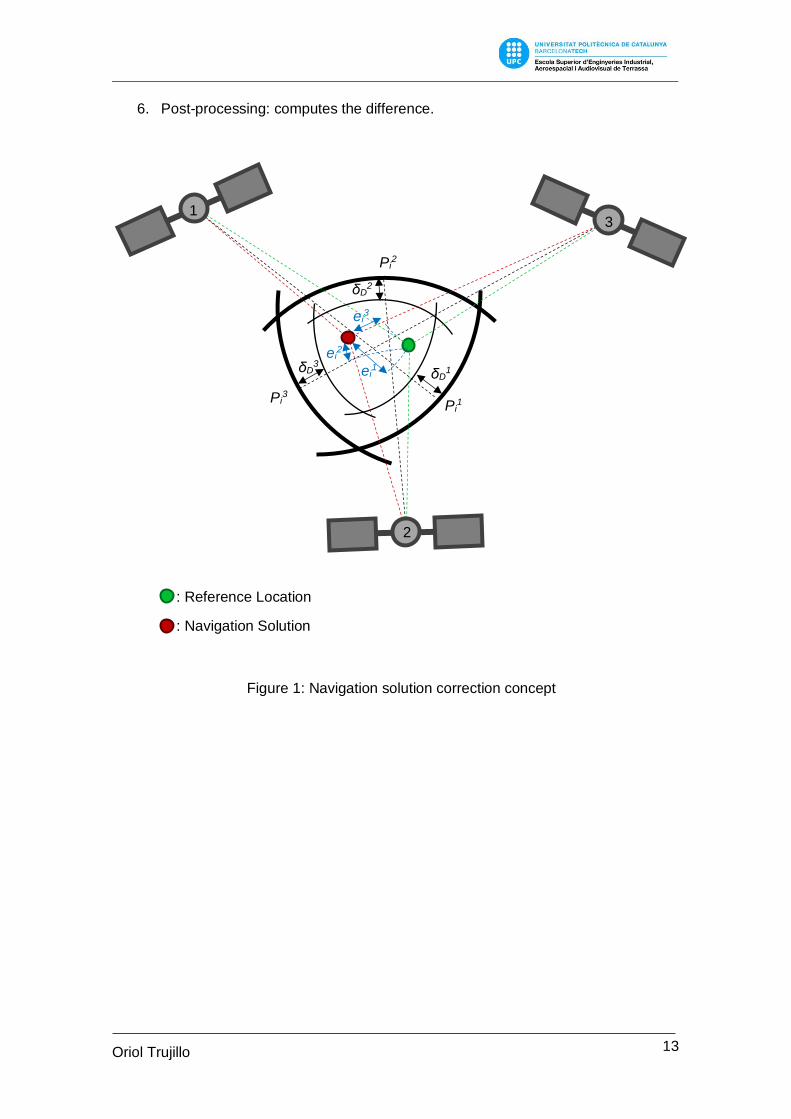
This section exposes an evolution of the latter methodology, where virtually generated
Space Vehicles have replaced real satellites. This yields a great advantage, so the
satellites can be placed wherever the user desires. Allowing an ideal satellite distribution,
can fix real problems such as the undesired high Vertical Dilution of precision (VDOP),
which is defined later in 6.2.1.2.5, so virtual satellites can be located even inside Earth.
Also the number of satellites used is chosen by the user, so the maximum potential of
this proposal can be achieved.
In this project, when this technique is applied, virtual satellites are located on a sphere
surface centred at the real base station position with a radius specified by the user2. Note
that satellites have a constant ECEF position (Earth-Centered Earth-Fixed coordinates),
which means they are rotating with the Earth and we always see them fixed at the same
position.
1 Pseudoranges are used only to find the final navigation solution. 2 Sometimes, if the radius is too low (~300m) convergence problems may occur.
Figure 2: Virtual Space Vehicles’ distribution (36 satellites, 1km of radius).
15 Oriol Trujillo
Martí
6.2.1.2.4 Computation of Receiver Position – Least Squares
Method
Once al pseudoranges have been corrected, it is time to recompute receiver position. To
do that, it has been performed an iteratively process on the linearized least squares
method. This process can be described as follows:
Variables legend
i: receiver i Pi
k: pseudorange from satellite k to receiver i3.
k: satellite k ρik: real geometric range between satellite k and receiver i.
m: total number of satellites.
dti: receiver clock offset
eik: residual error
Table 3: Variables lengend - Least squares method definition
𝑃𝑖𝑘 = 𝜌𝑖
𝑘 + 𝑐𝑑𝑡𝑖 + 𝑒𝑖𝑘 (6.9)
𝜌𝑖𝑘 = √(𝑋𝑘 − 𝑋𝑖)
2 + (𝑌𝑘 − 𝑌𝑖)2 + (𝑍𝑘 − 𝑍𝑖)
2 (6.10)
𝑃𝑖𝑘 = √(𝑋𝑘 − 𝑋𝑖)
2 + (𝑌𝑘 − 𝑌𝑖)2 + (𝑍𝑘 − 𝑍𝑖)
2 + 𝑐𝑑𝑡𝑖 + 𝑒𝑖𝑘 (6.11)
Where, if common DGPS corrections have been employed, the position of the satellite k
has to be corrected to compensate the Earth’s rotation as it is explained in section
6.2.1.4.
Linearizing equation (6.11):
𝑃𝑖𝑘 = 𝜌𝑖,𝑜
𝑘 −𝑋𝑘−𝑋𝑖,𝑜
𝜌𝑖,𝑜𝑘 −
𝑌𝑘−𝑌𝑖,𝑜
𝜌𝑖,𝑜𝑘 −
𝑍𝑘−𝑍𝑖,𝑜
𝜌𝑖,𝑜𝑘 + 𝑐𝑑𝑡𝑖 + 𝑒𝑖
𝑘 (6.12)
Where:
𝜌𝑖,𝑜𝑘 = √(𝑋𝑘 − 𝑋𝑖,𝑜)
2+ (𝑌𝑘 − 𝑌𝑖,𝑜)
2+ (𝑍𝑘 − 𝑍𝑖,𝑜)
2 (6.13)
3 It has been considered all corrections except for receiver clock offset
16 Oriol Trujillo
Martí
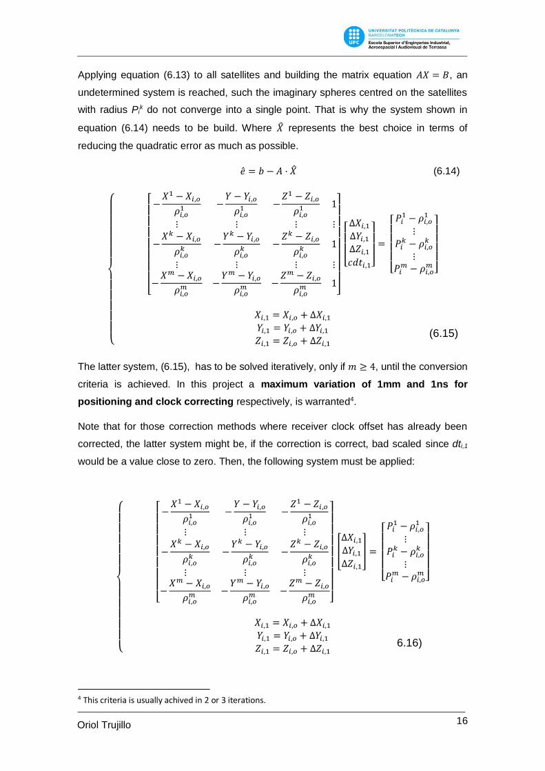
Applying equation (6.13) to all satellites and building the matrix equation 𝐴𝑋 = 𝐵, an
undetermined system is reached, such the imaginary spheres centred on the satellites
with radius Pik do not converge into a single point. That is why the system shown in
equation (6.14) needs to be build. Where represents the best choice in terms of
reducing the quadratic error as much as possible.
= 𝑏 − 𝐴 · (6.14)
[ −
𝑋1 − 𝑋𝑖,𝑜
𝜌𝑖,𝑜1 −
𝑌 − 𝑌𝑖,𝑜
𝜌𝑖,𝑜1 −
𝑍1 − 𝑍𝑖,𝑜
𝜌𝑖,𝑜1 1
⋮ ⋮ ⋮ ⋮
−𝑋𝑘 − 𝑋𝑖,𝑜
𝜌𝑖,𝑜𝑘
−𝑌𝑘 − 𝑌𝑖,𝑜
𝜌𝑖,𝑜𝑘
−𝑍𝑘 − 𝑍𝑖,𝑜
𝜌𝑖,𝑜𝑘
1
⋮ ⋮ ⋮ ⋮
−𝑋𝑚 − 𝑋𝑖,𝑜𝜌𝑖,𝑜𝑚 −
𝑌𝑚 − 𝑌𝑖,𝑜𝜌𝑖,𝑜𝑚 −
𝑍𝑚 − 𝑍𝑖,𝑜𝜌𝑖,𝑜𝑚 1
]
[ ∆𝑋𝑖,1∆𝑌𝑖,1∆𝑍𝑖,1𝑐𝑑𝑡𝑖,1]
=
[ 𝑃𝑖1 − 𝜌𝑖,𝑜
1
⋮𝑃𝑖𝑘 − 𝜌𝑖,𝑜
𝑘
⋮𝑃𝑖𝑚 − 𝜌𝑖,𝑜
𝑚]
𝑋𝑖,1 = 𝑋𝑖,𝑜 + ∆𝑋𝑖,1𝑌𝑖,1 = 𝑌𝑖,𝑜 + ∆𝑌𝑖,1𝑍𝑖,1 = 𝑍𝑖,𝑜 + ∆𝑍𝑖,1
The latter system, (6.15), has to be solved iteratively, only if 𝑚 ≥ 4, until the conversion
criteria is achieved. In this project a maximum variation of 1mm and 1ns for
positioning and clock correcting respectively, is warranted4.
Note that for those correction methods where receiver clock offset has already been
corrected, the latter system might be, if the correction is correct, bad scaled since dti,1
would be a value close to zero. Then, the following system must be applied:
[ −
𝑋1 − 𝑋𝑖,𝑜
𝜌𝑖,𝑜1 −
𝑌 − 𝑌𝑖,𝑜
𝜌𝑖,𝑜1 −
𝑍1 − 𝑍𝑖,𝑜
𝜌𝑖,𝑜1
⋮ ⋮ ⋮
−𝑋𝑘 − 𝑋𝑖,𝑜
𝜌𝑖,𝑜𝑘
−𝑌𝑘 − 𝑌𝑖,𝑜
𝜌𝑖,𝑜𝑘
−𝑍𝑘 − 𝑍𝑖,𝑜
𝜌𝑖,𝑜𝑘
⋮ ⋮ ⋮
−𝑋𝑚 − 𝑋𝑖,𝑜𝜌𝑖,𝑜𝑚 −
𝑌𝑚 − 𝑌𝑖,𝑜𝜌𝑖,𝑜𝑚 −
𝑍𝑚 − 𝑍𝑖,𝑜𝜌𝑖,𝑜𝑚
]
[
∆𝑋𝑖,1∆𝑌𝑖,1∆𝑍𝑖,1
] =
[ 𝑃𝑖1 − 𝜌𝑖,𝑜
1
⋮𝑃𝑖𝑘 − 𝜌𝑖,𝑜
𝑘
⋮𝑃𝑖𝑚 − 𝜌𝑖,𝑜
𝑚]
𝑋𝑖,1 = 𝑋𝑖,𝑜 + ∆𝑋𝑖,1𝑌𝑖,1 = 𝑌𝑖,𝑜 + ∆𝑌𝑖,1𝑍𝑖,1 = 𝑍𝑖,𝑜 + ∆𝑍𝑖,1
4 This criteria is usually achived in 2 or 3 iterations.
(6.15)
6.16)
17 Oriol Trujillo
Martí
Note that equation (6.16) can only be solved if the number of satellites is equal or higher
than 3, 𝑚 ≥ 3.
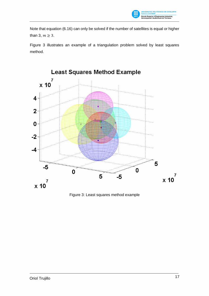
Figure 3 illustrates an example of a triangulation problem solved by least squares
method.
Figure 3: Least squares method example
18 Oriol Trujillo
Martí
6.2.1.2.5 Compute Dilution Of Precision
Once the final position has been calculated, Dilution Of Precision parameters can be
obtained from their definitions:
𝑄 = (𝐴𝑡 · 𝐴)−1 =1
𝜎02 ·
[ 𝜎𝑒2 𝜎𝑒𝑛 𝜎𝑒𝑢 𝜎𝑒,𝑐𝑑𝑡
𝜎𝑛𝑒 𝜎𝑛2 𝜎𝑛𝑢 𝜎𝑛,𝑐𝑑𝑡
𝜎𝑢𝑒 𝜎𝑢𝑛 𝜎𝑢2 𝜎𝑢,𝑐𝑑𝑡
𝜎𝑐𝑑𝑡,𝑒 𝜎𝑐𝑑𝑡,𝑛 𝜎𝑐𝑑𝑡,𝑢 𝜎𝑐𝑑𝑡2 ]
(6.17)
Geometric: 𝐺𝐷𝑂𝑃 = √𝑡𝑟(𝑄) (6.18)
Position: 𝑃𝐷𝑂𝑃 = √𝜎𝑒2+𝜎𝑛
2+𝜎𝑢2
𝜎02 (6.19)
Horizontal: 𝐻𝐷𝑂𝑃 = √𝜎𝑒2+𝜎𝑛
2
𝜎02 (6.20)
Vertical: 𝑉𝐷𝑂𝑃 =𝜎𝑢
𝜎0 (6.21)
Time: 𝑇𝐷𝑂𝑃 = 𝜎𝑐𝑑𝑡
𝜎0 (6.22)
Dilution of precision reflects the confidence of the method with its result. High values of
dilution of precision implies a wide region of possible solutions, and therefore, low
confidence.
6.2.1.3 Satellite positioning
As detailed in section A.1.6 of the annex A, each satellite position is determined by a
packet of ephemeris, which allows to estimate the Space Vehicle’s path until it is
updated.
In this section it is explained how to obtain ephemeris and satellite clock correction
parameters from the navigation message, and how to compute Space Vehicles’ position.
19 Oriol Trujillo
Martí
6.2.1.3.1 Navigation Message - Clock parameters and Ephemeris
The first step to compute the position of a satellite is to get clock correction parameters
and ephemeris. These parameters are extracted from the navigation message, which
structure is defined in [15], the most relevant information is pointed out in this section
and must be complemented with annex C since some tables has been omitted.
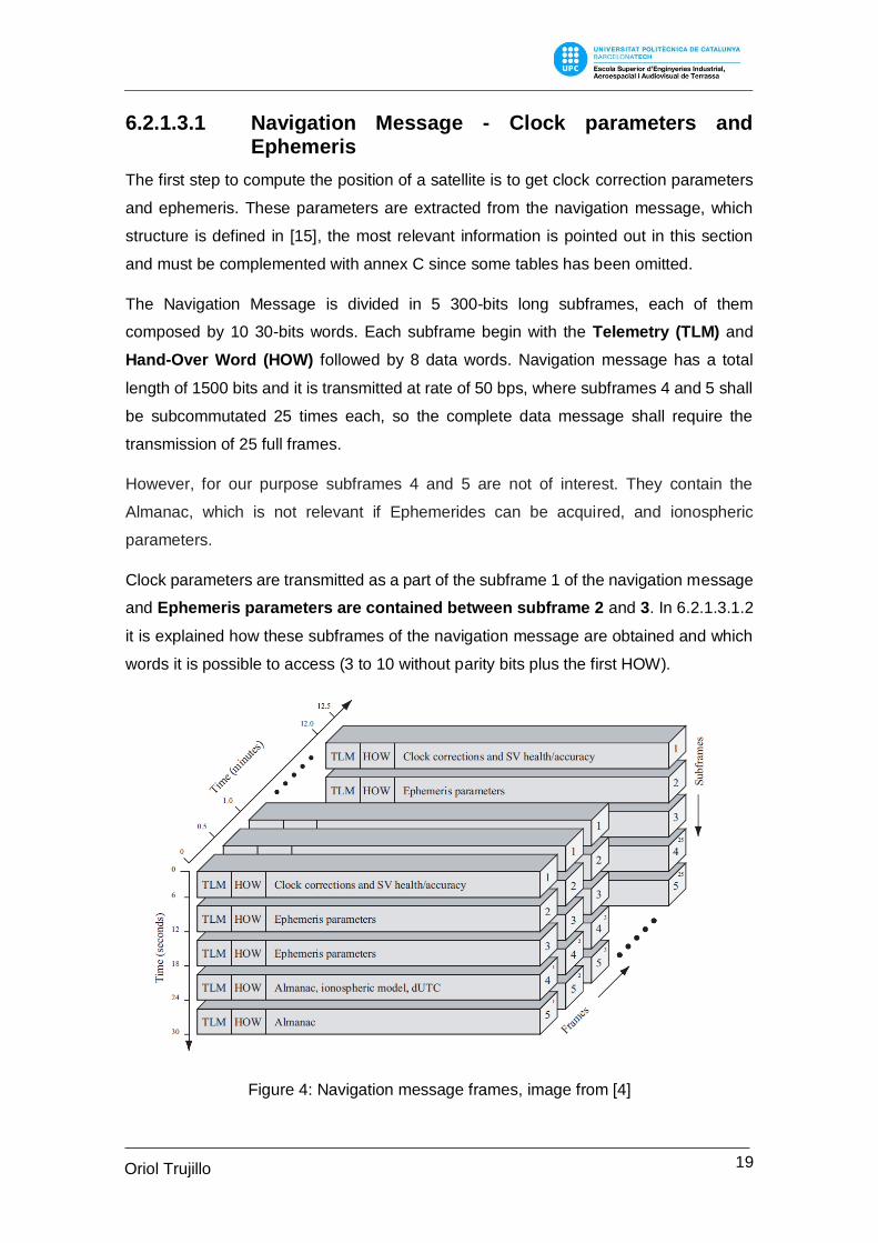
The Navigation Message is divided in 5 300-bits long subframes, each of them
composed by 10 30-bits words. Each subframe begin with the Telemetry (TLM) and
Hand-Over Word (HOW) followed by 8 data words. Navigation message has a total
length of 1500 bits and it is transmitted at rate of 50 bps, where subframes 4 and 5 shall
be subcommutated 25 times each, so the complete data message shall require the
transmission of 25 full frames.
However, for our purpose subframes 4 and 5 are not of interest. They contain the
Almanac, which is not relevant if Ephemerides can be acquired, and ionospheric
parameters.
Clock parameters are transmitted as a part of the subframe 1 of the navigation message
and Ephemeris parameters are contained between subframe 2 and 3. In 6.2.1.3.1.2
it is explained how these subframes of the navigation message are obtained and which
words it is possible to access (3 to 10 without parity bits plus the first HOW).
Figure 4: Navigation message frames, image from [4]
20 Oriol Trujillo
Martí
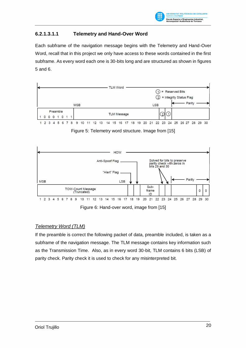
6.2.1.3.1.1 Telemetry and Hand-Over Word
Each subframe of the navigation message begins with the Telemetry and Hand-Over
Word, recall that in this project we only have access to these words contained in the first
subframe. As every word each one is 30-bits long and are structured as shown in figures
5 and 6.
Figure 5: Telemetry word structure. Image from [15]
Figure 6: Hand-over word, image from [15]
Telemetry Word (TLM)
If the preamble is correct the following packet of data, preamble included, is taken as a
subframe of the navigation message. The TLM message contains key information such
as the Transmission Time. Also, as in every word 30-bit, TLM contains 6 bits (LSB) of
parity check. Parity check it is used to check for any misinterpreted bit.
21 Oriol Trujillo
Martí
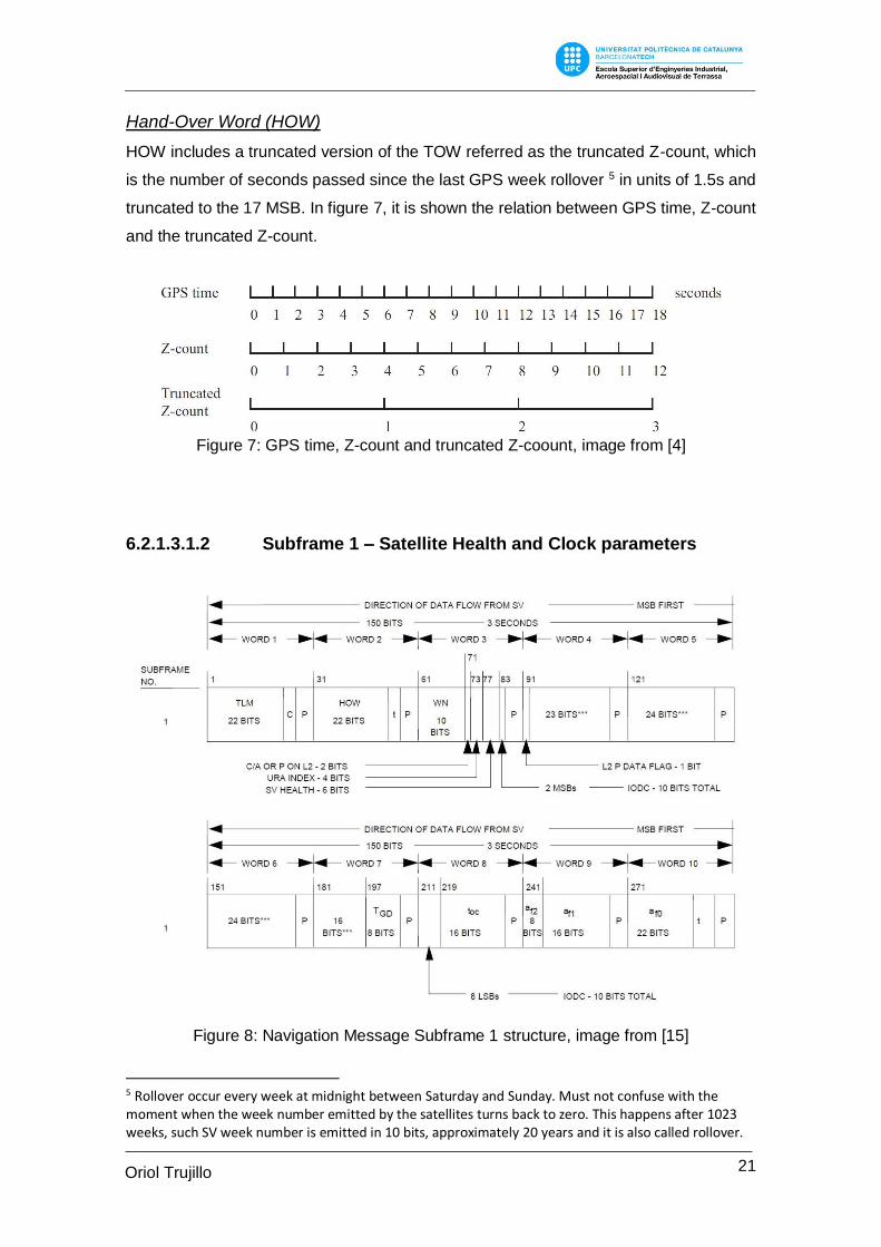
Hand-Over Word (HOW)
HOW includes a truncated version of the TOW referred as the truncated Z-count, which
is the number of seconds passed since the last GPS week rollover 5 in units of 1.5s and
truncated to the 17 MSB. In figure 7, it is shown the relation between GPS time, Z-count
and the truncated Z-count.
Figure 7: GPS time, Z-count and truncated Z-coount, image from [4]
6.2.1.3.1.2 Subframe 1 – Satellite Health and Clock parameters
Figure 8: Navigation Message Subframe 1 structure, image from [15]
5 Rollover occur every week at midnight between Saturday and Sunday. Must not confuse with the moment when the week number emitted by the satellites turns back to zero. This happens after 1023 weeks, such SV week number is emitted in 10 bits, approximately 20 years and it is also called rollover.

22 Oriol Trujillo
Martí
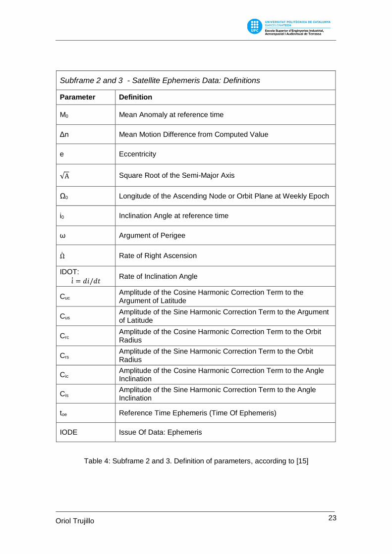
6.2.1.3.1.3 Subframe 2 and 3 – Satellite Ephemeris data
Figure 9: Navigation Message Subframe 2, image from [15]
Figure 10: Navigation Message Subframe 3, image from [15]
23 Oriol Trujillo
Martí
Subframe 2 and 3 - Satellite Ephemeris Data: Definitions
Parameter Definition
M0 Mean Anomaly at reference time
Δn Mean Motion Difference from Computed Value
e Eccentricity
√A Square Root of the Semi-Major Axis
Ω0 Longitude of the Ascending Node or Orbit Plane at Weekly Epoch
i0 Inclination Angle at reference time
ω Argument of Perigee
Ω Rate of Right Ascension
IDOT:
= 𝑑𝑖/𝑑𝑡 Rate of Inclination Angle
Cuc Amplitude of the Cosine Harmonic Correction Term to the Argument of Latitude
Cus Amplitude of the Sine Harmonic Correction Term to the Argument of Latitude
Crc Amplitude of the Cosine Harmonic Correction Term to the Orbit Radius
Crs Amplitude of the Sine Harmonic Correction Term to the Orbit Radius
Cic Amplitude of the Cosine Harmonic Correction Term to the Angle Inclination
Cis Amplitude of the Sine Harmonic Correction Term to the Angle Inclination
toe Reference Time Ephemeris (Time Of Ephemeris)
IODE Issue Of Data: Ephemeris
Table 4: Subframe 2 and 3. Definition of parameters, according to [15]
24 Oriol Trujillo
Martí
6.2.1.3.2 Satellite Clock and Time Correction
Receiver clock delay cannot be globally predicted such depends on each receiver clock,
which furthermore, is not very precise6, and it must be computed as an unknown with the
final position. However, the number of Space Vehicles of a GNSS constellation is limited
and satellite clocks are so much precise, if besides a correction of their small delay is
applied, the error introduced by these components is very low.
As explained in A.2.1 of annex A, each satellite clock delay is corrected with a second-
order polynomial which of parameters are given by the ephemeris. Time corrections are
applied as follows:
First let’s recall that pseudoranges are computes as:
𝑃𝑖𝑘 = 𝑐 · (𝑡𝑖 − 𝑡𝑘) = 𝑐 · 𝜏𝑖
𝑘 (6.23)
Where ti and tk are the measure of the arrival time to the receiver i and the emission time
of the satellite k respectively, measured by their own clocks. These measures might differ
from the GPS time at which that events really occurred. This can be expressed as:
𝑡𝑖 = 𝑡𝑖𝐺𝑃𝑆 + 𝑑𝑡𝑖 (6.24)
𝑡𝑘 = 𝑡𝑘𝐺𝑃𝑆 + 𝑑𝑡𝑘 (6.25)
Where dtk is the satellite clock delay given by the ephemeris defined in annex A section
A.2.2
𝑑𝑡𝑘 = 𝑎𝑓𝑜 + 𝑎𝑓1 · (𝑡𝑘 − 𝑡𝑜𝑒) + 𝑎𝑓2 · (𝑡
𝑘 − 𝑡𝑜𝑒)2 (6.26)7
And equation (7.1) can be rearranged as:
𝑡𝑘 = 𝑡𝑖 −𝑃𝑖𝑘
𝑐= 𝑡𝑖 − 𝜏𝑖
𝑘 (6.27)
Combining equation (7.3) and (7.5), tkGPS can be expressed as:
𝑡𝑘𝐺𝑃𝑆 = 𝑡𝑖 − 𝜏𝑖
𝑘 − 𝑑𝑡𝑘 (6.28)
Where tkGPS is the signal emission time referred at GPS time and, ti and τik are known
parameters.
6 Compared with Space Vehicles’ atomic clocks. 7 Note that relativistic effect is included in the bias parameter (a0).
25 Oriol Trujillo
Martí
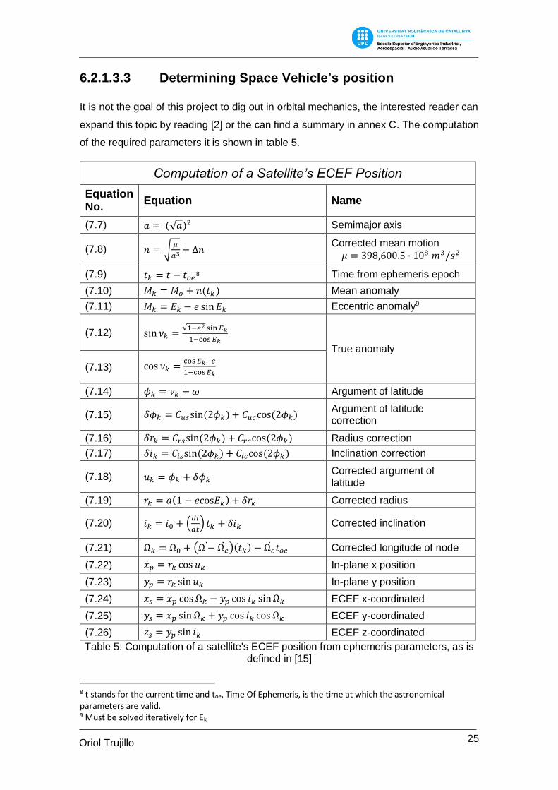
6.2.1.3.3 Determining Space Vehicle’s position
It is not the goal of this project to dig out in orbital mechanics, the interested reader can
expand this topic by reading [2] or the can find a summary in annex C. The computation
of the required parameters it is shown in table 5.
Computation of a Satellite’s ECEF Position
Equation No.
Equation Name
(7.7) 𝑎 = (√𝑎)2 Semimajor axis
(7.8) 𝑛 = √𝜇
𝑎3+ ∆𝑛
Corrected mean motion
𝜇 = 398,600.5 · 108 𝑚3/𝑠2
(7.9) 𝑡𝑘 = 𝑡 − 𝑡𝑜𝑒8 Time from ephemeris epoch
(7.10) 𝑀𝑘 = 𝑀𝑜 + 𝑛(𝑡𝑘) Mean anomaly
(7.11) 𝑀𝑘 = 𝐸𝑘 − 𝑒 sin𝐸𝑘 Eccentric anomaly9
(7.12) sin 𝜈𝑘 =√1−𝑒2 sin 𝐸𝑘
1−cos 𝐸𝑘
True anomaly
(7.13) cos 𝜈𝑘 =cos 𝐸𝑘−𝑒
1−cos𝐸𝑘
(7.14) 𝜙𝑘 = 𝜈𝑘 +𝜔 Argument of latitude
(7.15) 𝛿𝜙𝑘 = 𝐶𝑢𝑠sin (2𝜙𝑘) + 𝐶𝑢𝑐cos (2𝜙𝑘) Argument of latitude correction
(7.16) 𝛿𝑟𝑘 = 𝐶𝑟𝑠sin (2𝜙𝑘) + 𝐶𝑟𝑐cos (2𝜙𝑘) Radius correction
(7.17) 𝛿𝑖𝑘 = 𝐶𝑖𝑠sin (2𝜙𝑘) + 𝐶𝑖𝑐cos (2𝜙𝑘) Inclination correction
(7.18) 𝑢𝑘 = 𝜙𝑘 + 𝛿𝜙𝑘 Corrected argument of latitude
(7.19) 𝑟𝑘 = 𝑎(1 − 𝑒cos𝐸𝑘) + 𝛿𝑟𝑘 Corrected radius
(7.20) 𝑖𝑘 = 𝑖0 + (𝑑𝑖
𝑑𝑡) 𝑡𝑘 + 𝛿𝑖𝑘 Corrected inclination
(7.21) Ω𝑘 = Ω0 + (Ω − Ω)(𝑡𝑘) − Ω𝑡𝑜𝑒 Corrected longitude of node
(7.22) 𝑥𝑝 = 𝑟𝑘 cos 𝑢𝑘 In-plane x position
(7.23) 𝑦𝑝 = 𝑟𝑘 sin 𝑢𝑘 In-plane y position
(7.24) 𝑥𝑠 = 𝑥𝑝 cos Ω𝑘 − 𝑦𝑝 cos 𝑖𝑘 sinΩ𝑘 ECEF x-coordinated
(7.25) 𝑦𝑠 = 𝑥𝑝 sinΩ𝑘 + 𝑦𝑝 cos 𝑖𝑘 cos Ω𝑘 ECEF y-coordinated
(7.26) 𝑧𝑠 = 𝑦𝑝 sin 𝑖𝑘 ECEF z-coordinated
Table 5: Computation of a satellite's ECEF position from ephemeris parameters, as is defined in [15]
8 t stands for the current time and toe, Time Of Ephemeris, is the time at which the astronomical parameters are valid. 9 Must be solved iteratively for Ek
26 Oriol Trujillo
Martí
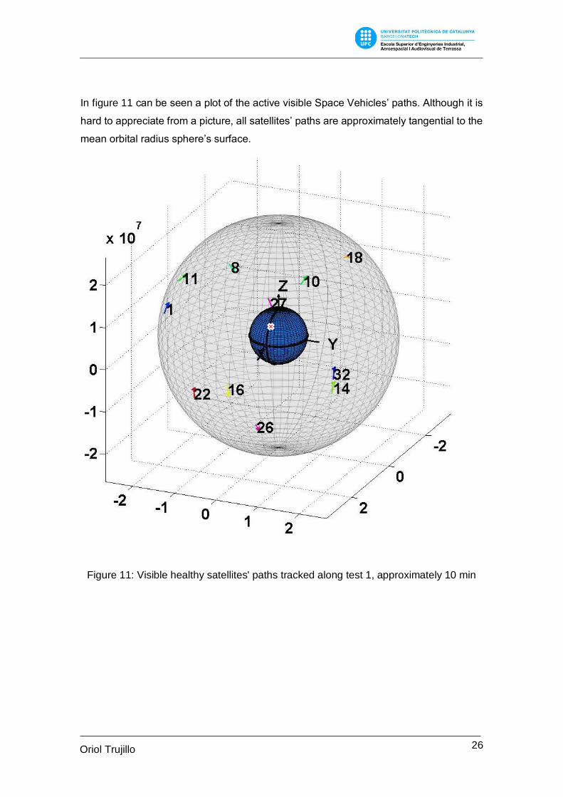
In figure 11 can be seen a plot of the active visible Space Vehicles’ paths. Although it is
hard to appreciate from a picture, all satellites’ paths are approximately tangential to the
mean orbital radius sphere’s surface.
Figure 11: Visible healthy satellites' paths tracked along test 1, approximately 10 min
27 Oriol Trujillo
Martí
6.2.1.4 Pseudorange Estimation
Pseudorange measurements are essential if DGPS corrections (the common method)
wants to be computed. As mentioned before, the available GPS receivers do not allow
to output raw data, so pseudoranges cannot be obtained as GPS output parameter and
must indirectly recomputed. That estimation can be performed if the active satellites’
positions, navigation final solution and Range Residuals are known.
Range Residuals is the parameter that relates the original measured pseudoranges with
the ranges between Space Vehicles and the navigation solution. It is a key parameter
for those correction methods that require information about the initial pseudoranges used
to compute the navigation solution. Range Residuals are defined, [16], as shown in
equation (6.29)
𝑅𝑎𝑛𝑔𝑒 𝑅𝑒𝑠𝑖𝑑𝑢𝑎𝑙𝑠 = 𝐶𝑎𝑙𝑐𝑢𝑙𝑎𝑡𝑒𝑑 𝑅𝑎𝑛𝑔𝑒 − 𝐸𝑠𝑡𝑖𝑚𝑎𝑡𝑒𝑑 𝑅𝑎𝑛𝑔𝑒 (6.29)
Understanding calculated range as the initial pseudorange before any correction and
estimated range as the range between the final solution and the satellite.
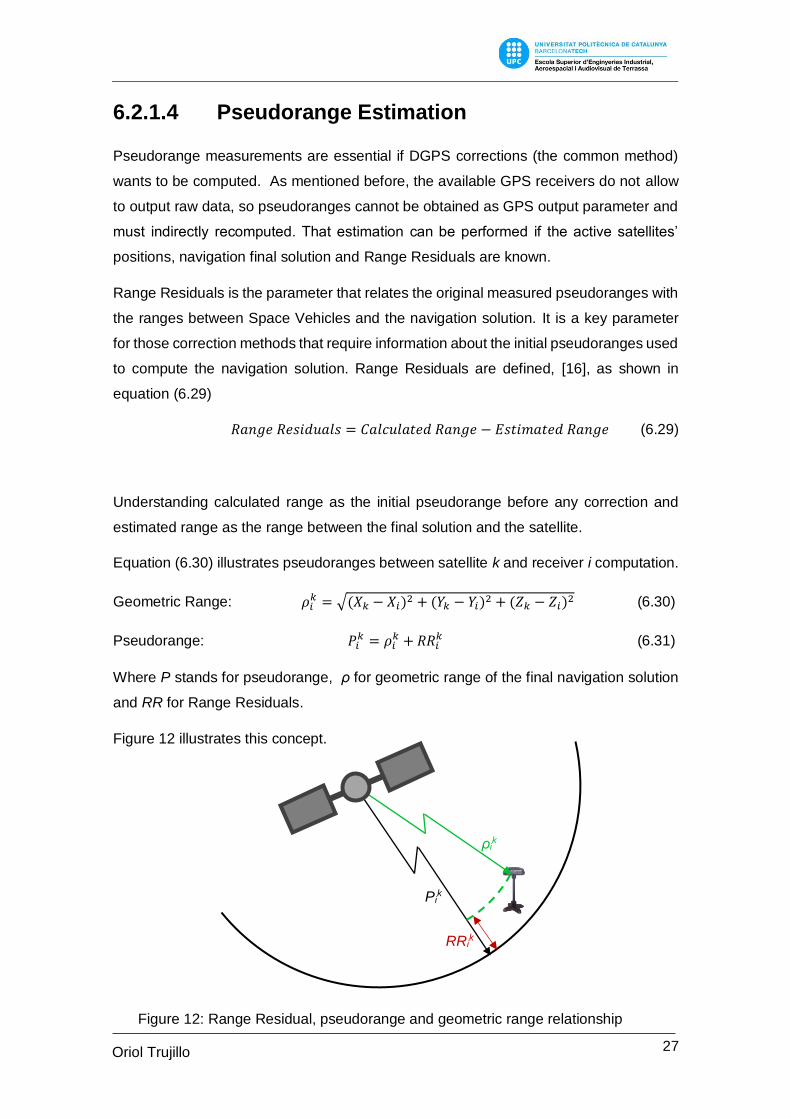
Equation (6.30) illustrates pseudoranges between satellite k and receiver i computation.
Geometric Range: 𝜌𝑖𝑘 = √(𝑋𝑘 − 𝑋𝑖)2 + (𝑌𝑘 − 𝑌𝑖)2 + (𝑍𝑘 − 𝑍𝑖)2 (6.30)
Pseudorange: 𝑃𝑖𝑘 = 𝜌𝑖
𝑘 + 𝑅𝑅𝑖𝑘 (6.31)
Where P stands for pseudorange, ρ for geometric range of the final navigation solution
and RR for Range Residuals.
Figure 12 illustrates this concept.
Pik
ρik
RRik
Figure 12: Range Residual, pseudorange and geometric range relationship
28 Oriol Trujillo
Martí
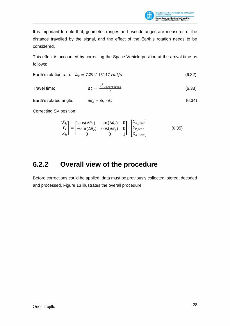
It is important to note that, geometric ranges and pseudoranges are measures of the
distance travelled by the signal, and the effect of the Earth’s rotation needs to be
considered.
This effect is accounted by correcting the Space Vehicle position at the arrival time as
follows:
Earth’s rotation rate: 𝑒 = 7.292115147 𝑟𝑎𝑑/𝑠 (6.32)
Travel time: ∆𝑡 = 𝜌𝑖_𝑢𝑛𝑐𝑜𝑟𝑟𝑒𝑐𝑡𝑒𝑑𝑘
𝑐 (6.33)
Earth’s rotated angle: ∆𝜃𝑒 = 𝑒 · ∆𝑡 (6.34)
Correcting SV position:
[𝑋𝑘𝑌𝑘𝑍𝑘
] = [cos (∆𝜃𝑒) sin (∆𝜃𝑒) 0−sin (∆𝜃𝑒) cos (∆𝜃𝑒) 0
0 0 1
] · [
𝑋𝑘_𝑢𝑛𝑐𝑌𝑘_𝑢𝑛𝑐𝑍𝑘_𝑢𝑛𝑐
] (6.35)
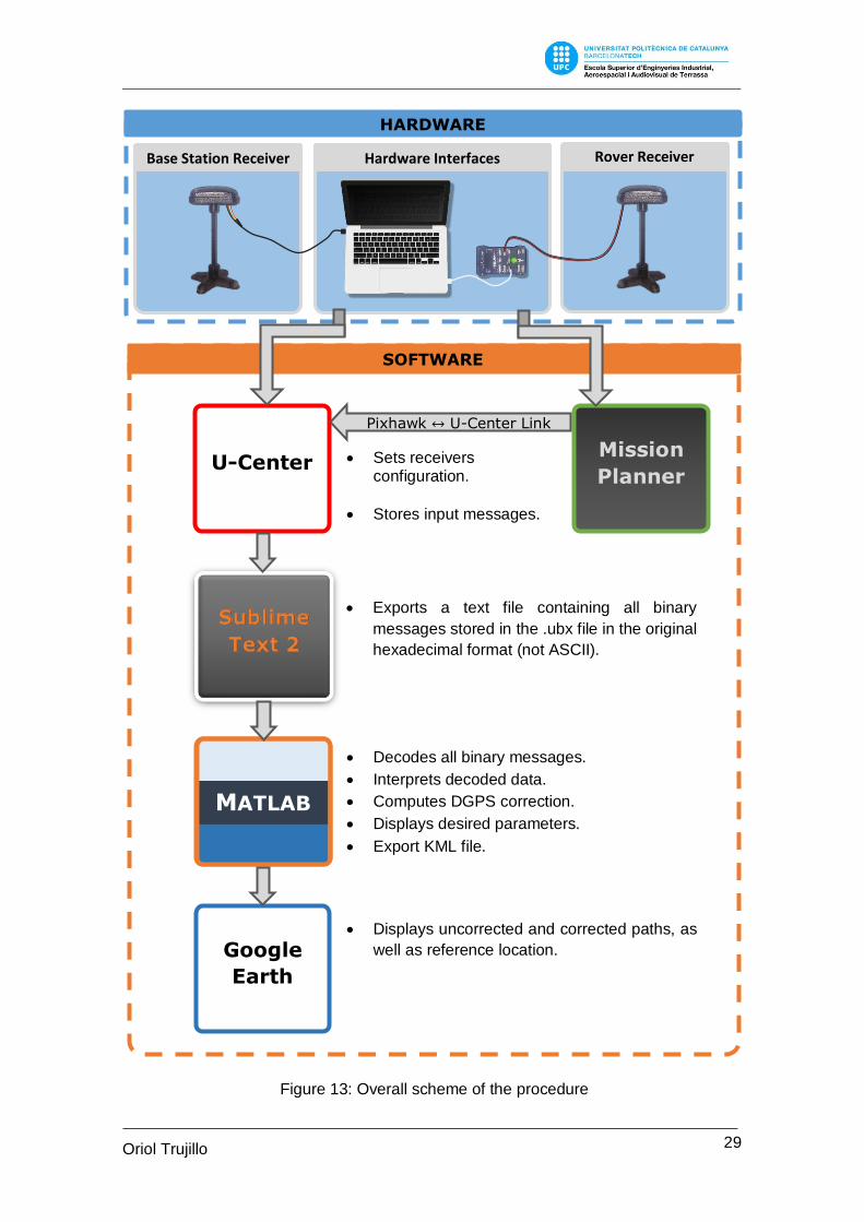
6.2.2 Overall view of the procedure
Before corrections could be applied, data must be previously collected, stored, decoded
and processed. Figure 13 illustrates the overall procedure.
29 Oriol Trujillo
Martí
HARDWARE
Hardware Interfaces Base Station Receiver Rover Receiver
SOFTWARE
Mission
Planner U-Center
Sublime
Text 2
MATLAB
Earth
Pixhawk ↔ U-Center Link
Sets receivers configuration.
Stores input messages.
Exports a text file containing all binary
messages stored in the .ubx file in the original
hexadecimal format (not ASCII).
Decodes all binary messages.
Interprets decoded data.
Computes DGPS correction.
Displays desired parameters.
Export KML file.
Displays uncorrected and corrected paths, as
well as reference location.
Figure 13: Overall scheme of the procedure

30 Oriol Trujillo
Martí
Note that, in figure 13 both receivers are connected, directly or indirectly, to the same
laptop. This is done when measures taken at the same location want to be compared,
which is the simplest test and the one taken as example. Section 7.2 exposes more
configurations.
31 Oriol Trujillo
Martí
7. Hardware and connections
In this section are detailed the main features of the GPS receivers, as well as the
elements that allow them to communicate with the laptop.
All hardware components involving this project are:
GPS receiver (x2)
APM 2.5 Flight Control Cable DF13 6 Position Connector (x2).
Pixhawk Autopilot
Standard USB to micro USB cable
USB to TTL-232R Serial cable
Laptop (x1 or x2)
Where the most important components (GPS receivers, Pixhawk and one of the APM
2.5 Flight Control Cable DF13 6 Position Connector) have been granted by the
Aerospace Department of ESEIAAT (UPC).
7.1 GPS receivers
The procedure followed to achieve the goal of the project, begins by acquiring
pseudoranges measurements and computing navigation solution (depending on the
correction method it is enough with the first process10). Both tasks are carried out by the
GPS receivers, whose good performances11 are essential for the success of the project.
The model of GPS receiver used in this project is the same for both, rover and base
station, and it is the 3DR U-Blox GPS with Compass Kit, which is based on U-Blox NEO-
7N GPS module and it is supplied by 3D Robotics. This model integrates the so-
10 Recall that pseudoranges are not transmitted to the user and must be estimated. 11 Understood as having good electronics, strong against interferences and internal noise, with low hardware delay, good sensitivity, etc.
32 Oriol Trujillo
Martí
mentioned U-Blox NEO-7N GPS module with the Taoglas GPS patch 1575 MHz antenna
and the HMC5883L digital compass.
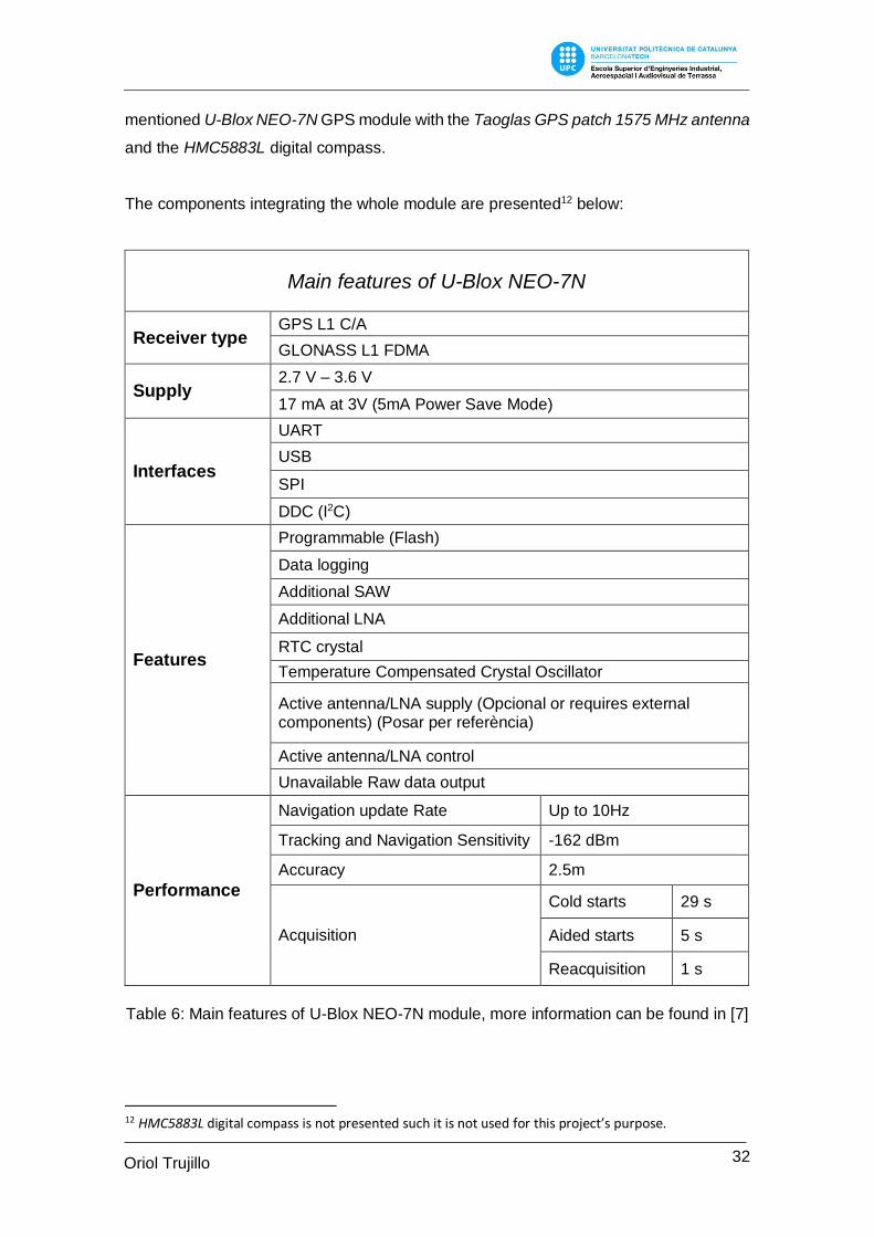
The components integrating the whole module are presented12 below:
Main features of U-Blox NEO-7N
Receiver type GPS L1 C/A
GLONASS L1 FDMA
Supply 2.7 V – 3.6 V
17 mA at 3V (5mA Power Save Mode)
Interfaces
UART
USB
SPI
DDC (I2C)
Features
Programmable (Flash)
Data logging
Additional SAW
Additional LNA
RTC crystal
Temperature Compensated Crystal Oscillator
Active antenna/LNA supply (Opcional or requires external components) (Posar per referència)
Active antenna/LNA control
Unavailable Raw data output
Performance
Navigation update Rate Up to 10Hz
Tracking and Navigation Sensitivity -162 dBm
Accuracy 2.5m
Acquisition
Cold starts 29 s
Aided starts 5 s
Reacquisition 1 s
Table 6: Main features of U-Blox NEO-7N module, more information can be found in [7]
12 HMC5883L digital compass is not presented such it is not used for this project’s purpose.
33 Oriol Trujillo
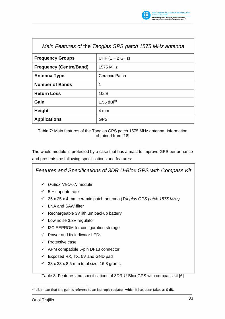
Martí
Main Features of the Taoglas GPS patch 1575 MHz antenna
Frequency Groups UHF (1 ~ 2 GHz)
Frequency (Centre/Band) 1575 MHz
Antenna Type Ceramic Patch
Number of Bands 1
Return Loss 10dB
Gain 1.55 dBi13
Height 4 mm
Applications GPS
Table 7: Main features of the Taoglas GPS patch 1575 MHz antenna, information
obtained from [18]
The whole module is protected by a case that has a mast to improve GPS performance
and presents the following specifications and features:
Features and Specifications of 3DR U-Blox GPS with Compass Kit
U-Blox NEO-7N module
5 Hz update rate
25 x 25 x 4 mm ceramic patch antenna (Taoglas GPS patch 1575 MHz)
LNA and SAW filter
Rechargeable 3V lithium backup battery
Low noise 3.3V regulator
I2C EEPROM for configuration storage
Power and fix indicator LEDs
Protective case
APM compatible 6-pin DF13 connector
Exposed RX, TX, 5V and GND pad
38 x 38 x 8.5 mm total size, 16.8 grams.
Table 8: Features and specifications of 3DR U-Blox GPS with compass kit [6]
13 dBi mean that the gain is refererd to an isotropic radiator, which it has been takes as 0 dB.
34 Oriol Trujillo
Martí
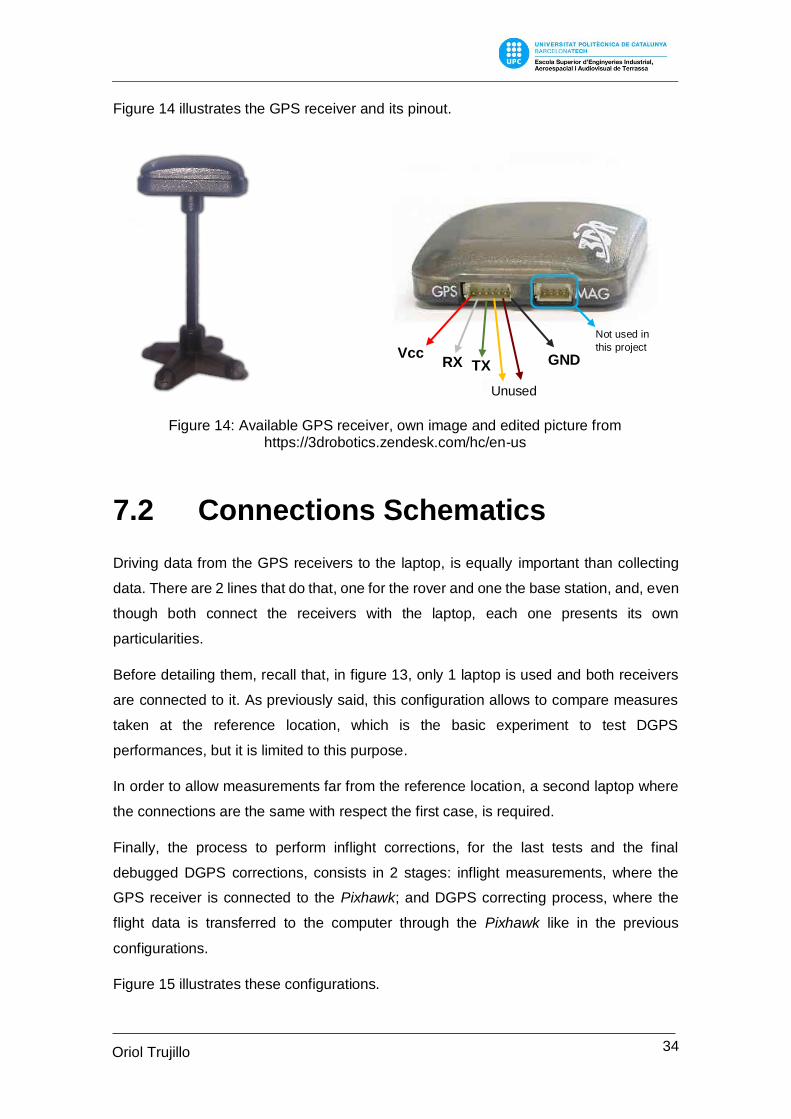
Figure 14 illustrates the GPS receiver and its pinout.
7.2 Connections Schematics
Driving data from the GPS receivers to the laptop, is equally important than collecting
data. There are 2 lines that do that, one for the rover and one the base station, and, even
though both connect the receivers with the laptop, each one presents its own
particularities.
Before detailing them, recall that, in figure 13, only 1 laptop is used and both receivers
are connected to it. As previously said, this configuration allows to compare measures
taken at the reference location, which is the basic experiment to test DGPS
performances, but it is limited to this purpose.
In order to allow measurements far from the reference location, a second laptop where
the connections are the same with respect the first case, is required.
Finally, the process to perform inflight corrections, for the last tests and the final
debugged DGPS corrections, consists in 2 stages: inflight measurements, where the
GPS receiver is connected to the Pixhawk; and DGPS correcting process, where the
flight data is transferred to the computer through the Pixhawk like in the previous
configurations.
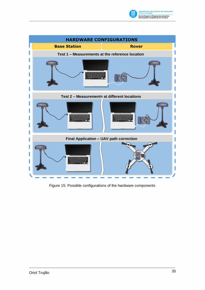
Figure 15 illustrates these configurations.
Vcc RX TX GND
Unused
Not used in
this project
Figure 14: Available GPS receiver, own image and edited picture from https://3drobotics.zendesk.com/hc/en-us
35 Oriol Trujillo
Martí
HARDWARE CONFIGURATIONS
Test 1 – Measurements at the reference location
Test 2 – Measurements at different locations
Final Application – UAV path correction
Base Station Rover
Figure 15: Possible configurations of the hardware components
36 Oriol Trujillo
Martí
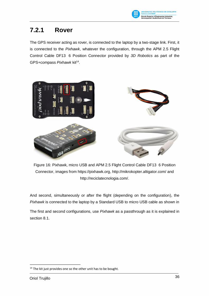
7.2.1 Rover
The GPS receiver acting as rover, is connected to the laptop by a two-stage link. First, it
is connected to the Pixhawk, whatever the configuration, through the APM 2.5 Flight
Control Cable DF13 6 Position Connector provided by 3D Robotics as part of the
GPS+compass Pixhawk kit14.
And second, simultaneously or after the flight (depending on the configuration), the
Pixhawk is connected to the laptop by a Standard USB to micro USB cable as shown in
The first and second configurations, use Pixhawk as a passthrough as it is explained in
section 8.1.
14 The kit just provides one so the other unit has to be bought.
Figure 16: Pixhawk, micro USB and APM 2.5 Flight Control Cable DF13 6 Position
Connector, images from https://pixhawk.org, http://mikrokopter.altigator.com/ and
http://reciclatecnologia.com/.
37 Oriol Trujillo
Martí
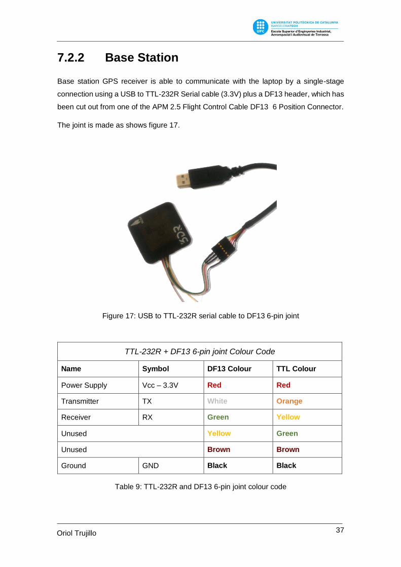
7.2.2 Base Station
Base station GPS receiver is able to communicate with the laptop by a single-stage
connection using a USB to TTL-232R Serial cable (3.3V) plus a DF13 header, which has
been cut out from one of the APM 2.5 Flight Control Cable DF13 6 Position Connector.
The joint is made as shows figure 17.
Figure 17: USB to TTL-232R serial cable to DF13 6-pin joint
TTL-232R + DF13 6-pin joint Colour Code
Name Symbol DF13 Colour TTL Colour
Power Supply Vcc – 3.3V Red Red
Transmitter TX White Orange
Receiver RX Green Yellow
Unused Yellow Green
Unused Brown Brown
Ground GND Black Black
Table 9: TTL-232R and DF13 6-pin joint colour code
38 Oriol Trujillo
Martí
There reasons why base station and rover connections are different and they are not
both connected through Pixhawks or TTL-232R Serial cables are exposed next.
The first case is not possible because the localhost cannot attend multiple requests at
the same time. Furthermore, it is enough waste of resources using once a so capable
device such as Pixhawk just as a passthrough.
Upon the second case, as previously said, to make this last cable, 2 components are
required, a USB to TTL-232R Serial cable and a APM 2.5 Flight Control Cable DF13 6
Position Connector. This means time and money, so it has been arrived to an optimal
solution.
39 Oriol Trujillo
Martí
8. Software
In the whole project four different software have been required in three different steps to
reach the final solution and one more to visualize it. Each of them explained below.
8.1 Mission Planner
Mission Planner is an open-source ground station application for planes, copters or
rovers using a compatible flight controllers such as ArduPilot, Multiwii or Pixhawk. It is
capable of monitoring telemetry in real time, analyse flight data after flying, plan
autonomous missions or arm the aircraft.
None of that functionalities have been used in this project but another very important
one.
As previously said, Mission Planner can interact with the Pixhawk autopilot, where the
rover GPS receiver is connected to. So it allows to read stored GPS data for computing
corrections, if the flight configuration is set, or, in lack of a pair of FTDI cables, it acts as
a link between rover GPS receiver and U-Center for the ground-based configurations.
This is possible due to Mission Planner allows to create an exclusive passthrough for the
GPS at localhost port 500, where U-Center has access to.
8.2 U-Center
U-Center is a software developed by U-Blox used as interface of U-Blox GNSS receivers.
It allows to monitor receivers’ performance in reals time, as well as to set up their desired
configuration and store the data got from the receivers.
It is able to display all messages that receivers are allowed to send but it is not possible
to work with the input data. This fact adds value to the implemented code.
40 Oriol Trujillo
Martí
8.2.1 Messages and Protocols
U-Center can read and understand data coming from receiver coded in two protocols,
NMEA and UBX. Combining the information obtained from some key messages coded
in these protocols, it has been possible to implement this project. Understanding
messages’ structure is crucial in the decoding process. Next, are introduced receivers’
protocols and those messages that have been used or had any utility at some point.
However, each message’s structure must be perfectly known such it can be decoded,
the full description of these messages is detailed in annex D and can be also found in
[19].
8.2.1.1 NMEA
NMEA protocol is the specification within GPS receiver communication is defined. It was
developed by the National Marine Electronics Association (NMEA) to define the interface
between marine electronic equipment [16].
NMEA format it is defined by lines of data called sentences that contains totally self-
contained information. Each sentence begin with dollar symbol ‘$’ and ends with an
asterisk ‘*’ followed by two checksum hexadecimal numbers. Message information is
ASCII coded text contained between those characters in a single line. It begins with a
pair of letters that identifies the GNSS type followed by three more specifying the
message class. The content fields sent by each message is separated by commas until
the checksum and it cannot be longer than 80 visible characters plus the line terminators.
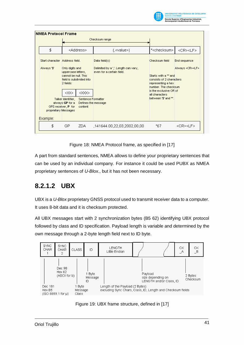
NMEA sentences general structure it is shown in figure 18.
41 Oriol Trujillo
Martí
Figure 18: NMEA Protocol frame, as specified in [17]
A part from standard sentences, NMEA allows to define your proprietary sentences that
can be used by an individual company. For instance it could be used PUBX as NMEA
proprietary sentences of U-Blox., but it has not been necessary.
8.2.1.2 UBX
UBX is a U-Blox proprietary GNSS protocol used to transmit receiver data to a computer.
It uses 8-bit data and it is checksum protected.
All UBX messages start with 2 synchronization bytes (B5 62) identifying UBX protocol
followed by class and ID specification. Payload length is variable and determined by the
own message through a 2-byte length field next to ID byte.
Figure 19: UBX frame structure, defined in [17]
42 Oriol Trujillo
Martí
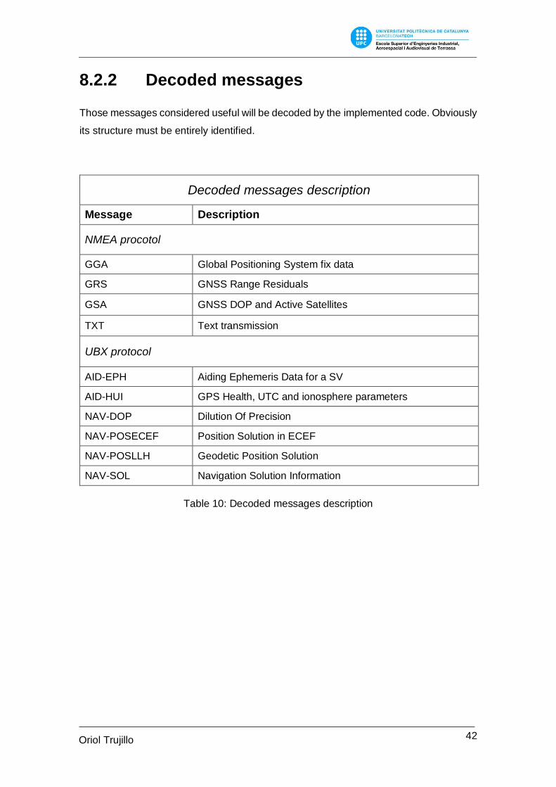
8.2.2 Decoded messages
Those messages considered useful will be decoded by the implemented code. Obviously
its structure must be entirely identified.
Decoded messages description
Message Description
NMEA procotol
GGA Global Positioning System fix data
GRS GNSS Range Residuals
GSA GNSS DOP and Active Satellites
TXT Text transmission
UBX protocol
AID-EPH Aiding Ephemeris Data for a SV
AID-HUI GPS Health, UTC and ionosphere parameters
NAV-DOP Dilution Of Precision
NAV-POSECEF Position Solution in ECEF
NAV-POSLLH Geodetic Position Solution
NAV-SOL Navigation Solution Information
Table 10: Decoded messages description
43 Oriol Trujillo
Martí
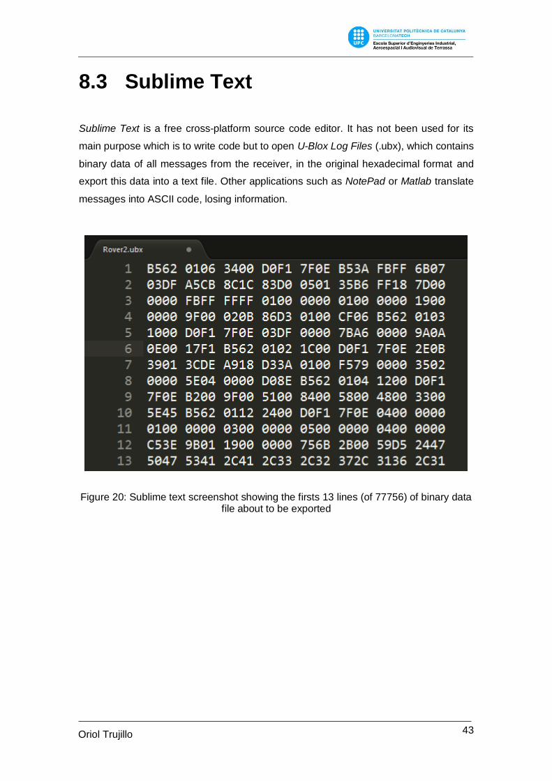
8.3 Sublime Text
Sublime Text is a free cross-platform source code editor. It has not been used for its
main purpose which is to write code but to open U-Blox Log Files (.ubx), which contains
binary data of all messages from the receiver, in the original hexadecimal format and
export this data into a text file. Other applications such as NotePad or Matlab translate
messages into ASCII code, losing information.
Figure 20: Sublime text screenshot showing the firsts 13 lines (of 77756) of binary data
file about to be exported
44 Oriol Trujillo
Martí
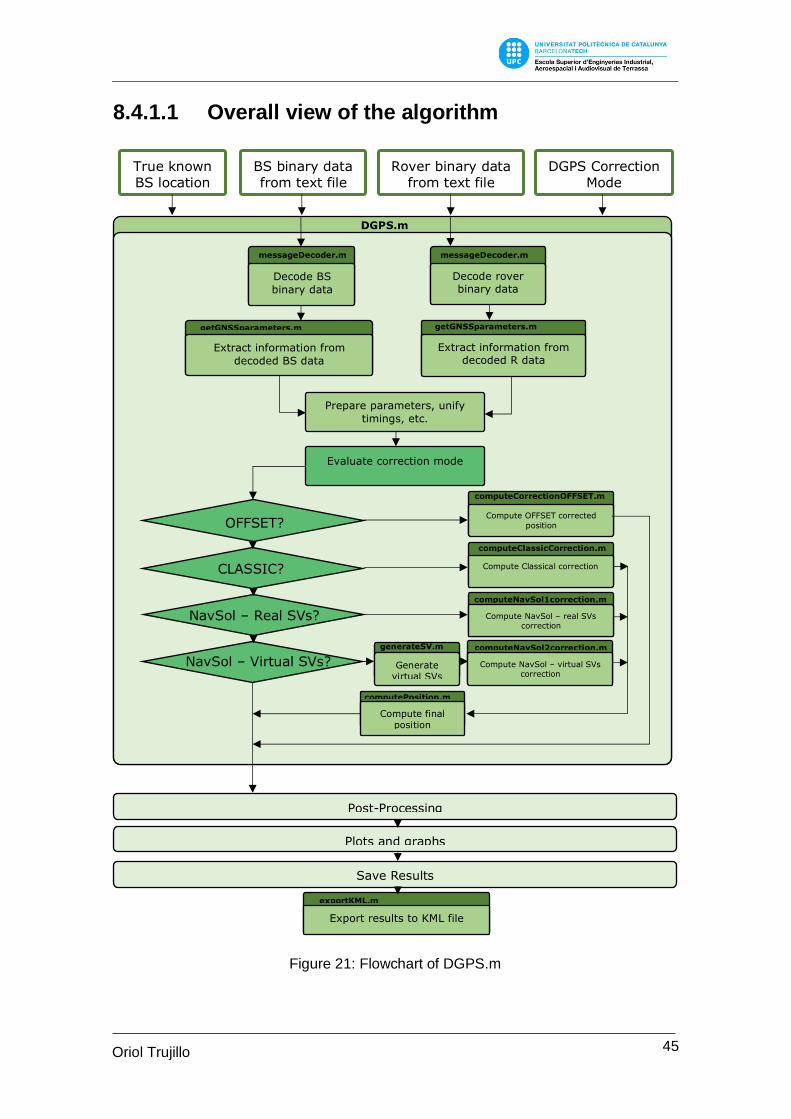
8.4 Implemented MATLAB Code
In this section, it is presented the implemented code based on MATLAB that performs
all the tasks previously exposed. The code reads and decodes the input text files,
rover and base station, according to protocols’ guidelines exposed in 8.2.1 and annex D.
From the decoded binary data the information is extracted and processed. All the date
is properly classified in structures and the user has access to all received and processed
data. Along this preparation stage data is verified, satellites are tracked, timings are
unified, and so on. Then the selected correcting method is applied and position
recomputed (if pseudorange domain corrections are demanded), according to section
6.2.1. After all, results are plotted, saved and into a KML file.
Even though this task has consumed the major part of the time, only the most important
functions are presented through flowcharts in order to keep an adequate extension of
the report and the interest of the reader. All functions, except graphs and post-
processing, and the main structures, used to store and deal with the decoded data, are
detailed in annexes E and F respectively.
This has been the largest and more complex task, not only because of the code
implementation but the extensive validation process that has been submitted.
8.4.1 Flowcharts
Note that, the flowcharts have been simplified, otherwise it would result excessively large
and unclear.15
Also, it has been drawn as parallel processes some tasks that could be performed at the
same time if enough computers work together. In the current code version this is not
contemplated.
15 For instance, the code has some tools to prevent user mistakes and internal errors that are not shown in the flowcharts.
45 Oriol Trujillo
Martí
8.4.1.1 Overall view of the algorithm
True known BS location
BS binary data from text file
Rover binary data from text file
DGPS Correction Mode
DGPS.m
Decode BS
binary data
messageDecoder.m
Decode rover binary data
messageDecoder.m
Extract information from
decoded BS data
getGNSSparameters.m
Extract information from decoded R data
getGNSSparameters.m
Evaluate correction mode
Prepare parameters, unify
timings, etc.
NavSol – Real SVs?
NavSol – Virtual SVs? Generate virtual SVs
generateSV.m
Compute final position
computePosition.m
Compute OFFSET corrected
position
computeCorrectionOFFSET.m
Compute Classical correction
computeClassicCorrection.m
Compute NavSol – real SVs correction
computeNavSol1correction.m
Compute NavSol – virtual SVs correction
computeNavSol2correction.m
Post-Processing
Plots and graphs
Save Results
Export results to KML file
exportKML.m
OFFSET?
CLASSIC?
Figure 21: Flowchart of DGPS.m
46 Oriol Trujillo
Martí
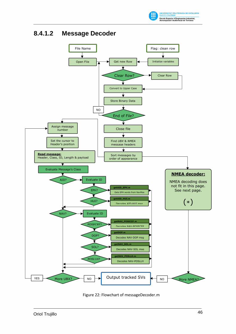
8.4.1.2 Message Decoder
File Name Flag: clean row
Open File Initialize variables Get new Row
Clear Row
Convert to Upper Case
Store Binary Data
Close file
Find UBX & NMEA
message headers
Sort messages by order of appearance
NO
Assign message number
Set the cursor to
Header’s position
Read message:
Header, Class, ID, Length & payload
Evaluate Message’s Class
AID? Evaluate ID
EPH?
?
HUI?
?
NAV? Evaluate ID
Gets EPH words from NavMsg
getAID_EPH.m
Decodes AID-HUI msg
getAID_HUI.m
POSECEF?
DOP?
Decodes NAV-POSECEF
msg
getNAV_POSECEF.m
Decodes NAV-DOP msg
getDOP.m
SOL?
Decodes NAV-SOL msg
getNAV_SOL.m
POSLLH?
Decodes NAV-POSLLH msg
getNAV_POSLLH.m
YES Output tracked SVs NO More NMEA? NO
NMEA decoder:
NMEA decoding does not fit in this page.
See next page.
(*)
End of File?
Clear Row?
More UBX?
Figure 22: Flowchart of messageDecoder.m
47 Oriol Trujillo
Martí
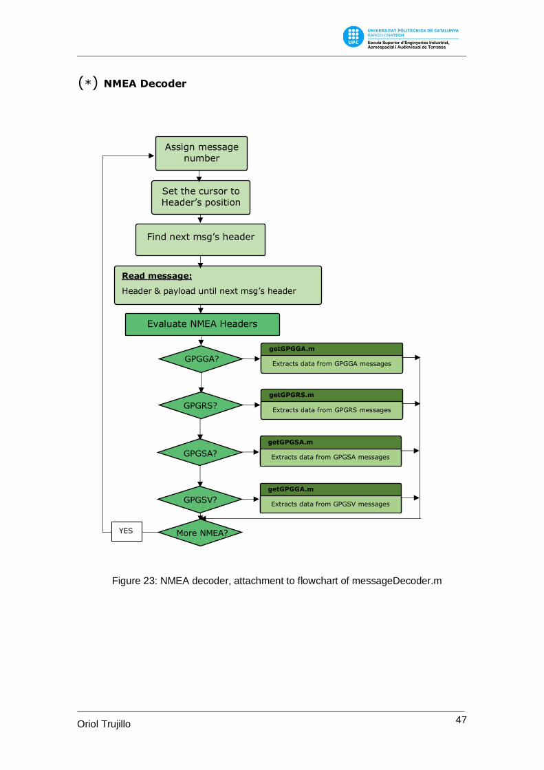
(*) NMEA Decoder
Assign message number
Set the cursor to Header’s position
Read message:
Header & payload until next msg’s header
Evaluate NMEA Headers
More NMEA?
Find next msg’s header
Extracts data from GPGGA messages
getGPGGA.m
GPGGA?
Extracts data from GPGRS messages
getGPGRS.m
GPGRS?
Extracts data from GPGSA messages
getGPGSA.m
GPGSA?
Extracts data from GPGSV messages
getGPGGA.m
GPGSV?
YES
Figure 23: NMEA decoder, attachment to flowchart of messageDecoder.m
48 Oriol Trujillo
Martí
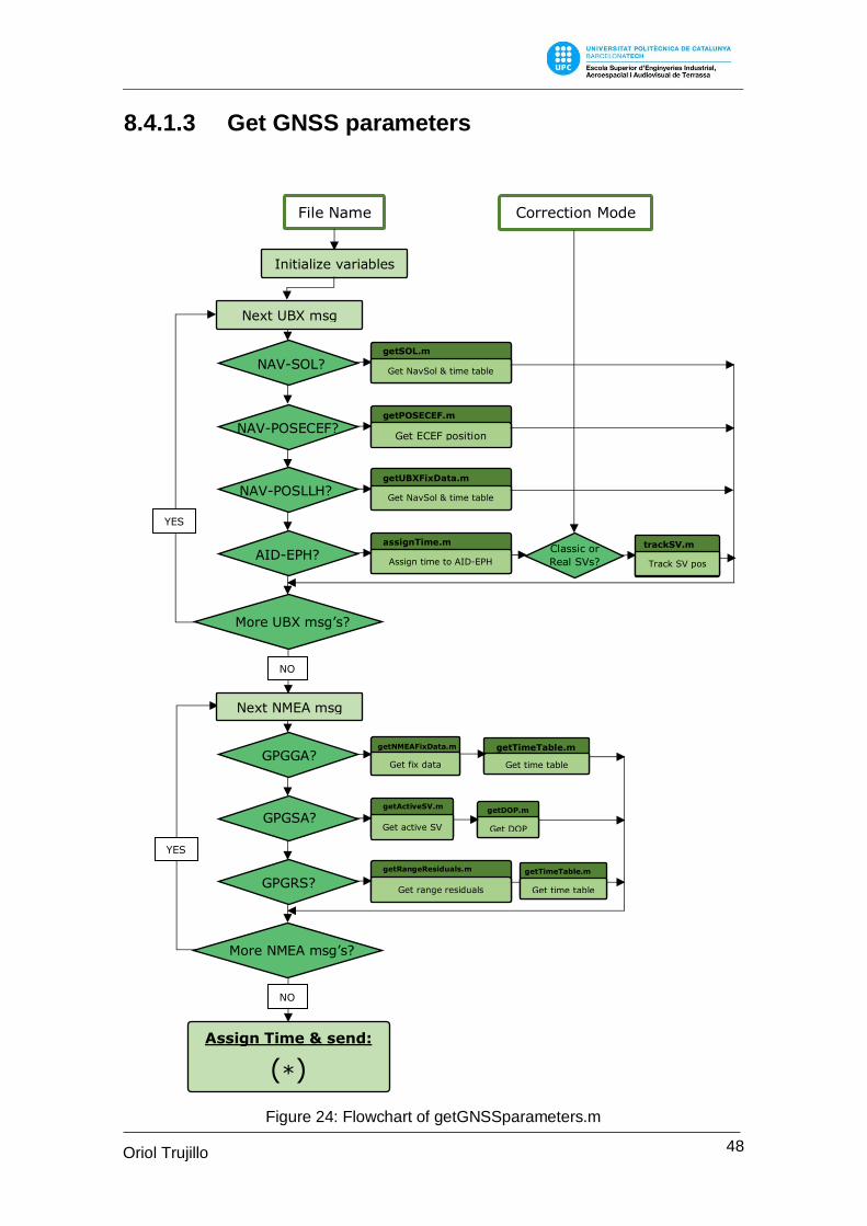
8.4.1.3 Get GNSS parameters
Next NMEA msg
GPGGA? Get fix data
getNMEAFixData.m
GPGSA? Get active SV
getActiveSV.m
GPGRS? Get range residuals
getRangeResiduals.m
More NMEA msg’s?
YES
Get time table
getTimeTable.m
Get DOP
getDOP.m
Get time table
getTimeTable.m
NO
NO
Assign Time & send:
(*)
File Name Correction Mode
Initialize variables
Next UBX msg
NAV-SOL? Get NavSol & time table
getSOL.m
NAV-POSECEF? Get ECEF position
getPOSECEF.m
NAV-POSLLH? Get NavSol & time table
getUBXFixData.m
AID-EPH? Assign time to AID-EPH
assignTime.m
Track SV pos
trackSV.m
More UBX msg’s?
YES
Classic or
Real SVs?
Figure 24: Flowchart of getGNSSparameters.m
49 Oriol Trujillo
Martí
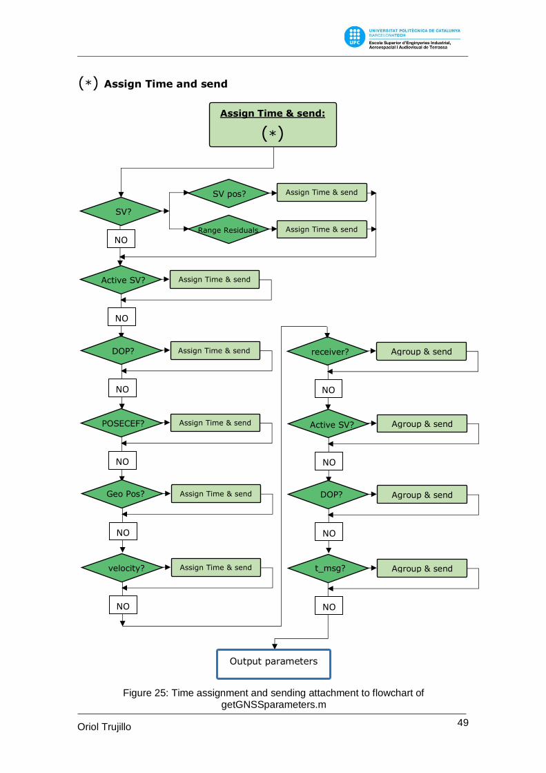
(*) Assign Time and send
Assign Time & send:
(*)
NO
SV?
SV pos?
Range Residuals
Assign Time & send
Assign Time & send
Active SV? Assign Time & send
NO
DOP? Assign Time & send
NO
POSECEF? Assign Time & send
NO
Geo Pos? Assign Time & send
NO
velocity? Assign Time & send
NO
receiver? Agroup & send
NO
Active SV? Agroup & send
NO
DOP? Agroup & send
NO
t_msg? Agroup & send
NO
Output parameters
Figure 25: Time assignment and sending attachment to flowchart of getGNSSparameters.m
50 Oriol Trujillo
Martí
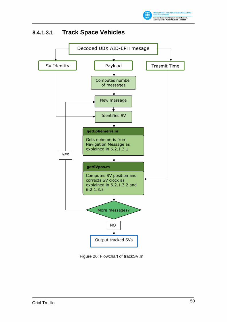
8.4.1.3.1 Track Space Vehicles
Decoded UBX AID-EPH mesage
SV Identity Payload Trasmit Time
Gets ephemeris from Navigation Message as
explained in 6.2.1.3.1
getEphemeris.m
Computes SV position and corrects SV clock as explained in 6.2.1.3.2 and 6.2.1.3.3
getSVpos.m
Computes number of messages
New message
More messages?
Output tracked SVs
Identifies SV
NO
YES
Figure 26: Flowchart of trackSV.m

51 Oriol Trujillo
Martí
8.4.1.4 Time Coordination
Each message is received in different moments and provide information of different
instants. However, it is necessary to perform corrections to coordinate those parameters
such as rover, base station and Space Vehicle position, active satellites, ionosphere
information, etc.
To do that, it has been taken as a reference base station UBX NAV-SOL messages,
because provide accurate TOW, and the other parameters have been linearly
interpolated to fit base station navigation solution time. The unification has been
performed in the correction rank, this is the interval of time when all the parameters
required to compute and apply the corrections provide valid information.
The routine implemented works as follows:
Reference Structure Structure
Extract Time array New Instant
Property fits
reference?
Get upper & lower closest times plus locations in the structure.
closestValue.m
Linear interpolation of specified fields:
𝑝𝑟𝑜𝑝𝑐𝑜𝑟𝑟(𝑗) = 𝑝𝑟𝑜𝑝(𝑙𝑜𝑤𝐿𝑜𝑐). 𝑓𝑖𝑒𝑙𝑑1 +𝑟𝑒𝑓𝑒𝑟𝑒𝑛𝑐𝑒(𝑖). 𝑓𝑖𝑒𝑙𝑑1 − 𝑙𝑜𝑤𝑇𝑖𝑚𝑒
𝑢𝑝𝑇𝑖𝑚𝑒 − 𝑙𝑜𝑤𝑇𝑖𝑚𝑒· (𝑝𝑟𝑜𝑝(𝑢𝑝𝐿𝑜𝑐). 𝑓𝑖𝑒𝑙𝑑1. 𝑝𝑟𝑜𝑝(𝑙𝑜𝑤𝐿𝑜𝑐). 𝑓𝑖𝑒𝑙𝑑1)
Output propcorr
Figure 27: Flowchart of time coordination
52 Oriol Trujillo
Martí
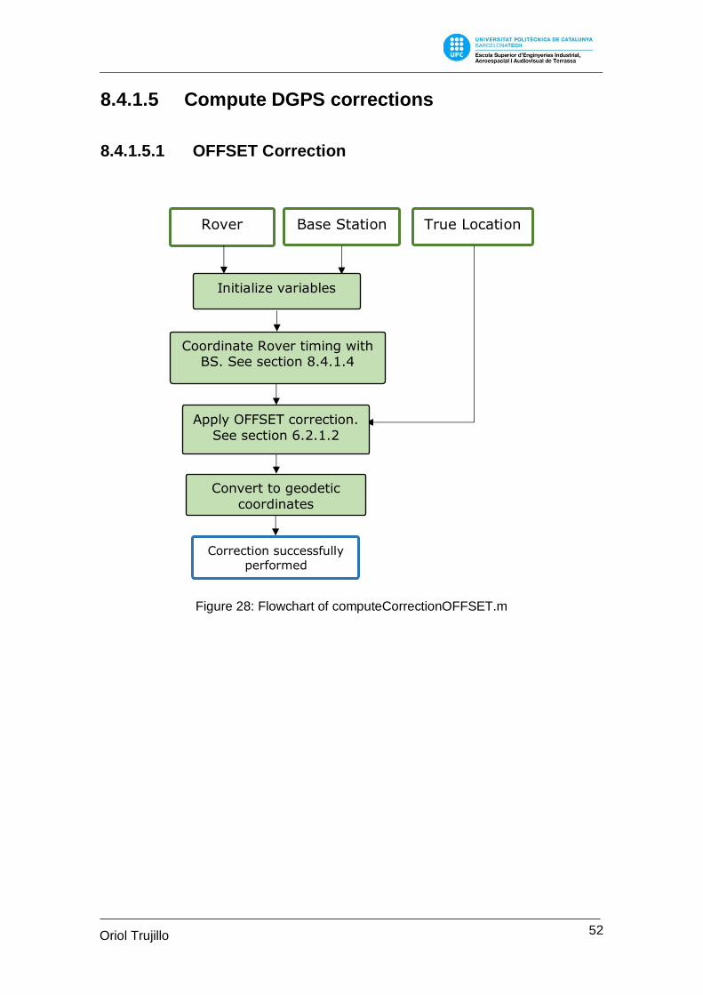
8.4.1.5 Compute DGPS corrections
8.4.1.5.1 OFFSET Correction
Rover Base Station
Coordinate Rover timing with BS. See section 8.4.1.4
Initialize variables
True Location
Convert to geodetic
coordinates
Correction successfully
performed
Apply OFFSET correction.
See section 6.2.1.2
Figure 28: Flowchart of computeCorrectionOFFSET.m
53 Oriol Trujillo
Martí
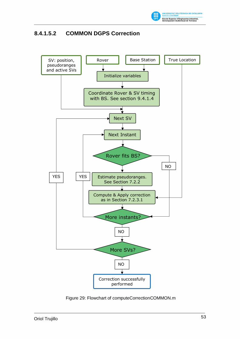
8.4.1.5.2 COMMON DGPS Correction
Rover Base Station True Location
Initialize variables
Coordinate Rover & SV timing
with BS. See section 9.4.1.4
Next SV
Next Instant
More instants?
NO
More SVs?
NO
Correction successfully performed
SV: position, pseudoranges and active SVs
Compute & Apply correction as in Section 7.2.3.1
Rover fits BS?
YES YES Estimate pseudoranges. See Section 7.2.2
NO
Figure 29: Flowchart of computeCorrectionCOMMON.m
54 Oriol Trujillo
Martí
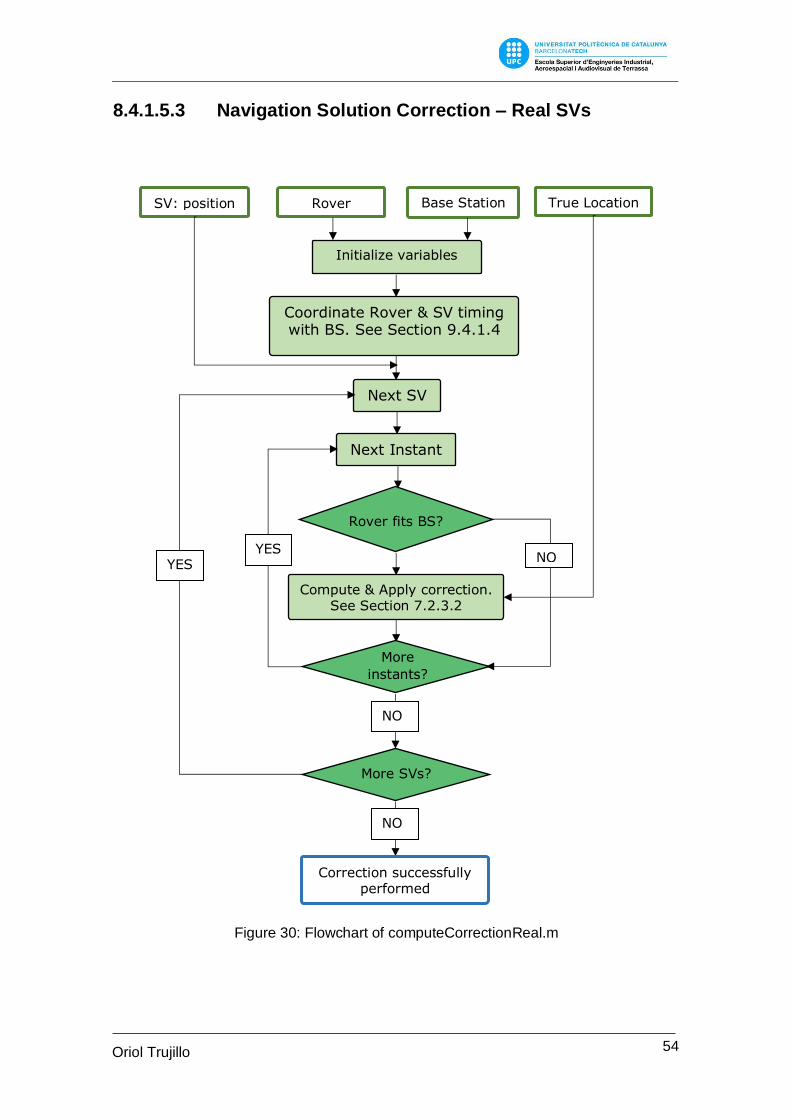
8.4.1.5.3 Navigation Solution Correction – Real SVs
Rover Base Station True Location SV: position
Initialize variables
Coordinate Rover & SV timing with BS. See Section 9.4.1.4
Next SV
Next Instant
Compute & Apply correction. See Section 7.2.3.2
More
instants?
NO
More SVs?
NO
Correction successfully performed
YES
YES
Rover fits BS?
NO
Figure 30: Flowchart of computeCorrectionReal.m
55 Oriol Trujillo
Martí
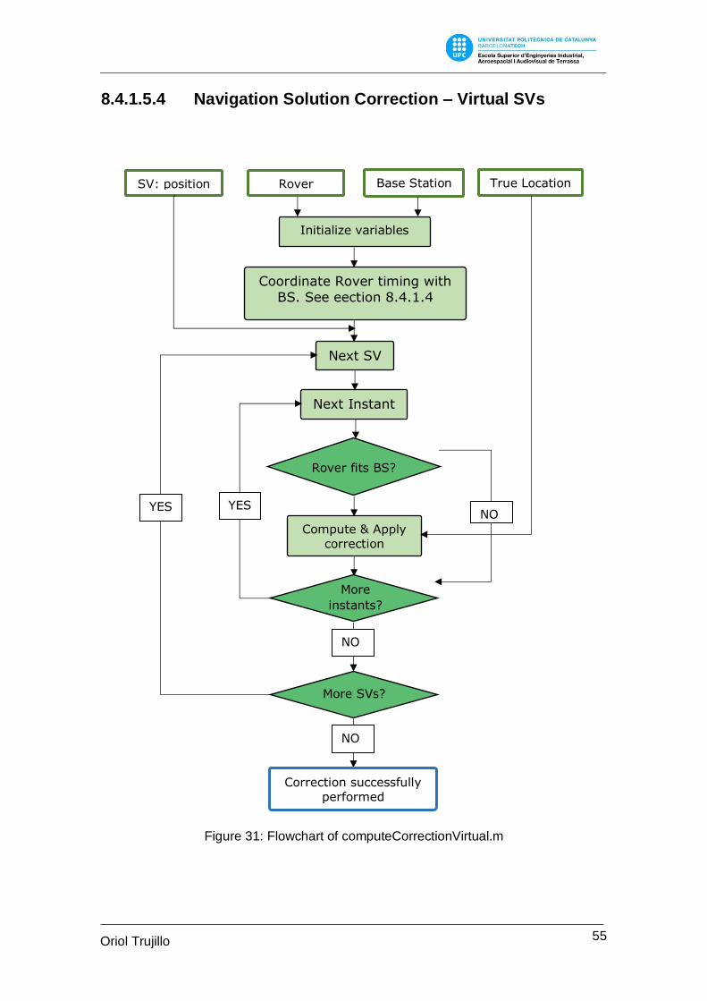
8.4.1.5.4 Navigation Solution Correction – Virtual SVs
Rover Base Station True Location SV: position
Initialize variables
Coordinate Rover timing with
BS. See eection 8.4.1.4
Next SV
Next Instant
Compute & Apply correction
More
instants?
NO
More SVs?
NO
Correction successfully performed
YES YES
Rover fits BS?
NO
Figure 31: Flowchart of computeCorrectionVirtual.m

56 Oriol Trujillo
Martí
8.4.1.6 Compute Position
Rover: position SV: position &
corrected pseudorange
Get max # of rows
New Instant / Row
Evaluate correction mode
CLASSIC? Computes minimum
quadratic error solution. See section 8.4.1.7
leastSquarePos.m
NavSol – Real SVs?
Computes minimum quadratic error solution. See section 8.4.1.7
leastSquarePosNOdt.m
NavSol – Virtual SVs?
Assign Time
n < Total#Rows?
YES
NO
Position successfully completed
Figure 32: Flowchart of computePosition.m
57 Oriol Trujillo
Martí
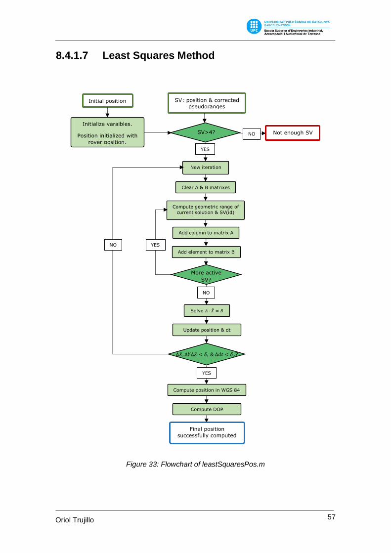
8.4.1.7 Least Squares Method
Initial position
Initialize varaibles.
Position initialized with
rover position.
SV: position & corrected pseudoranges
Not enough SV NO
YES
SV>4?
New iteration
Clear A & B matrixes
Compute geometric range of
current solution & SV(id)
Add column to matrix A
Add element to matrix B
More active
SV?
YES
NO
Solve 𝐴 · = 𝐵
Update position & dt
∆𝑋, ∆𝑌∆𝑍 < 𝛿1 & ∆𝑑𝑡 < 𝛿2?
NO
YES
Compute position in WGS 84
Compute DOP
Final position
successfully computed
Figure 33: Flowchart of leastSquaresPos.m
58 Oriol Trujillo
Martí
8.5 Google Earth
Thanks to this powerful tool, it is not required an expensive cartographic equipment to
get the reference coordinates, since Google Earth allows the user to get the geographic
coordinates of the reference location, as well as, once the results have been obtained
and exported, it allows to visualize the corrected and uncorrected 3D paths on the map,
so it is easy to check the effectivity of each method.
Google Earth’s 3D map is obtained by the superimposition of images from satellite
imagery, aerial photography and geographic information. Of course, it has a limited
accuracy and the obtained coordinates for the given coordinates may differ from their
true values and the solution given by the GPS receiver.
Actually this fact does not matter, due to the correction methods overcome this error.
Since measurements are corrected based on the reference position, and it is taken from
Google Earth, all coordinates get referred to this, that at the end are exported this 3D
map again.

59 Oriol Trujillo
Martí
9. Results
Once the methodologies has been introduced, described and implemented, it is time to
test them.
9.1 Test design
Before proceeding to perform the field work, it is necessary to design the experiment.
The location, duration and receivers’ configuration have been considered.
9.1.1 Selection of Location
A very relevant factor to consider while designing the experiments, it’s the location where
they are going to be performed. It is important to highlight two aspects that need to be
taken into account while selecting it.
The first one is that the experimentation needs to be developed into an open area with
the minimum obstacles. Ensuring this, the effect of multipath reflections and shadowing
will be minimized, as well as a good satellite coverture is warranted. This consideration
does not compromises the fidelity of the test with the real application since agrees with
the desired flight environment.
The other element to consider is that in order to get an accurate reference, as it is got
from Google Earth, the selected environment should have a recognizable reference
element.
The selected location for testing satisfies both requirements, it is spotted in the middle of
a wide avenue surrounded by much separated low buildings without any near disturbing
obstacle. The exact situation is between Sant Feliu de Llobregat and Sant Joan Despí,
in front of the sports complex Ciutat Esportiva Joan Gamper, where a given post has
been taken as reference.
The coordinates of the reference location are:
60 Oriol Trujillo
Martí
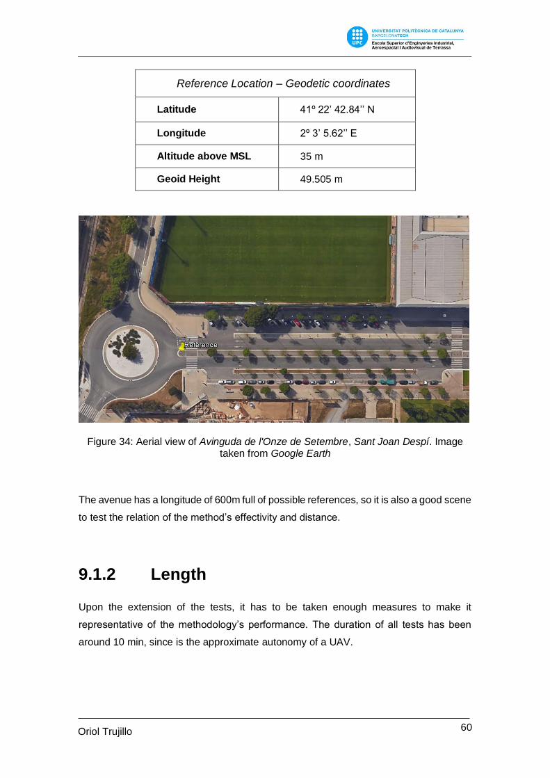
Reference Location – Geodetic coordinates
Latitude 41º 22’ 42.84’’ N
Longitude 2º 3’ 5.62’’ E
Altitude above MSL 35 m
Geoid Height 49.505 m
Figure 34: Aerial view of Avinguda de l'Onze de Setembre, Sant Joan Despí. Image taken from Google Earth
The avenue has a longitude of 600m full of possible references, so it is also a good scene
to test the relation of the method’s effectivity and distance.
9.1.2 Length
Upon the extension of the tests, it has to be taken enough measures to make it
representative of the methodology’s performance. The duration of all tests has been
around 10 min, since is the approximate autonomy of a UAV.
61 Oriol Trujillo
Martí
9.1.3 Message configuration
Before proceeding to start the test, each GPS receiver needs to be configure it using U-
Center. In the configuration process has to be defined the baud rate, the output protocols,
the output messages, and so on.
The requested messages depend on the correction mode that is going to be used. If the
program ignored the messages that are not required for the current correction method.
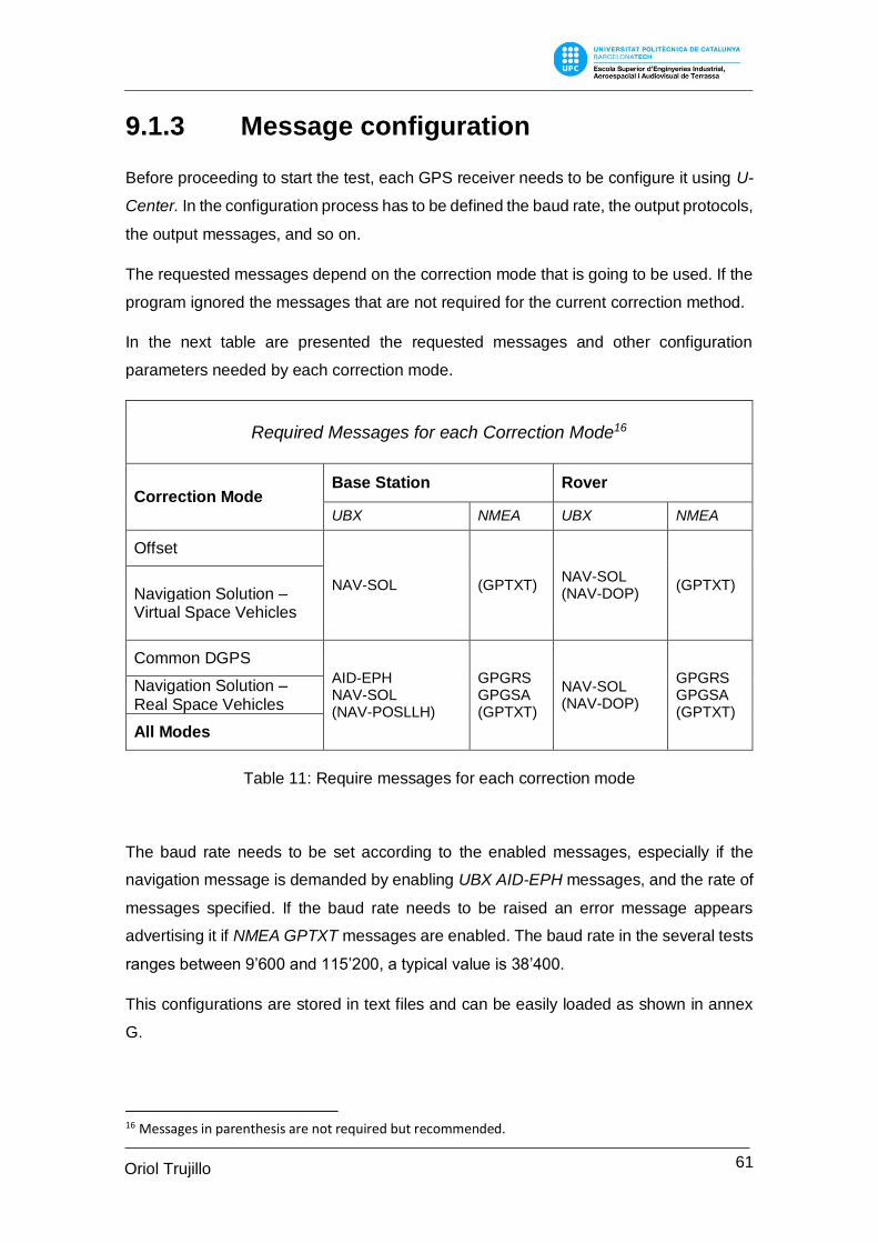
In the next table are presented the requested messages and other configuration
parameters needed by each correction mode.
Required Messages for each Correction Mode16
Correction Mode Base Station Rover
UBX NMEA UBX NMEA
Offset
NAV-SOL (GPTXT) NAV-SOL (NAV-DOP)
(GPTXT) Navigation Solution – Virtual Space Vehicles
Common DGPS
AID-EPH NAV-SOL (NAV-POSLLH)
GPGRS GPGSA (GPTXT)
NAV-SOL (NAV-DOP)
GPGRS GPGSA (GPTXT)
Navigation Solution – Real Space Vehicles
All Modes
Table 11: Require messages for each correction mode
The baud rate needs to be set according to the enabled messages, especially if the
navigation message is demanded by enabling UBX AID-EPH messages, and the rate of
messages specified. If the baud rate needs to be raised an error message appears
advertising it if NMEA GPTXT messages are enabled. The baud rate in the several tests
ranges between 9’600 and 115’200, a typical value is 38’400.
This configurations are stored in text files and can be easily loaded as shown in annex
G.
16 Messages in parenthesis are not required but recommended.
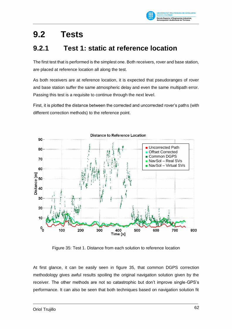
62 Oriol Trujillo
Martí
9.2 Tests
9.2.1 Test 1: static at reference location
The first test that is performed is the simplest one. Both receivers, rover and base station,
are placed at reference location all along the test.
As both receivers are at reference location, it is expected that pseudoranges of rover
and base station suffer the same atmospheric delay and even the same multipath error.
Passing this test is a requisite to continue through the next level.
First, it is plotted the distance between the corrected and uncorrected rover’s paths (with
different correction methods) to the reference point.
Figure 35: Test 1. Distance from each solution to reference location
At first glance, it can be easily seen in figure 35, that common DGPS correction
methodology gives awful results spoiling the original navigation solution given by the
receiver. The other methods are not so catastrophic but don’t improve single-GPS’s
performance. It can also be seen that both techniques based on navigation solution fit
Uncorrected Path Offset Corrected Common DGPS NavSol – Real SVs NavSol – Virtual SVs
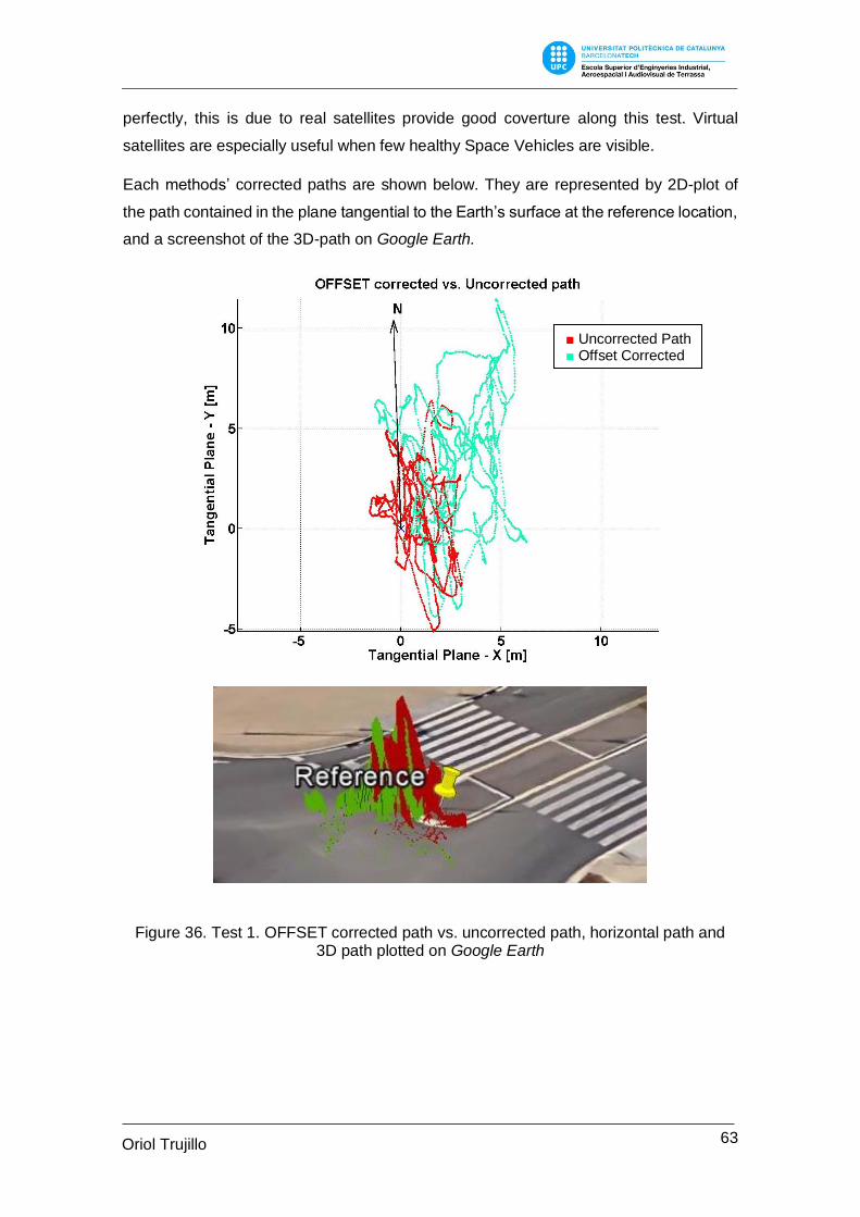
63 Oriol Trujillo
Martí
perfectly, this is due to real satellites provide good coverture along this test. Virtual
satellites are especially useful when few healthy Space Vehicles are visible.
Each methods’ corrected paths are shown below. They are represented by 2D-plot of
the path contained in the plane tangential to the Earth’s surface at the reference location,
and a screenshot of the 3D-path on Google Earth.
Figure 36. Test 1. OFFSET corrected path vs. uncorrected path, horizontal path and
3D path plotted on Google Earth
Uncorrected Path Offset Corrected
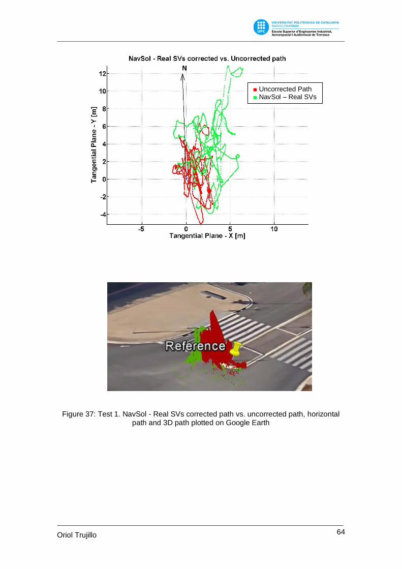
64 Oriol Trujillo
Martí
Uncorrected Path NavSol – Real SVs
Figure 37: Test 1. NavSol - Real SVs corrected path vs. uncorrected path, horizontal path and 3D path plotted on Google Earth
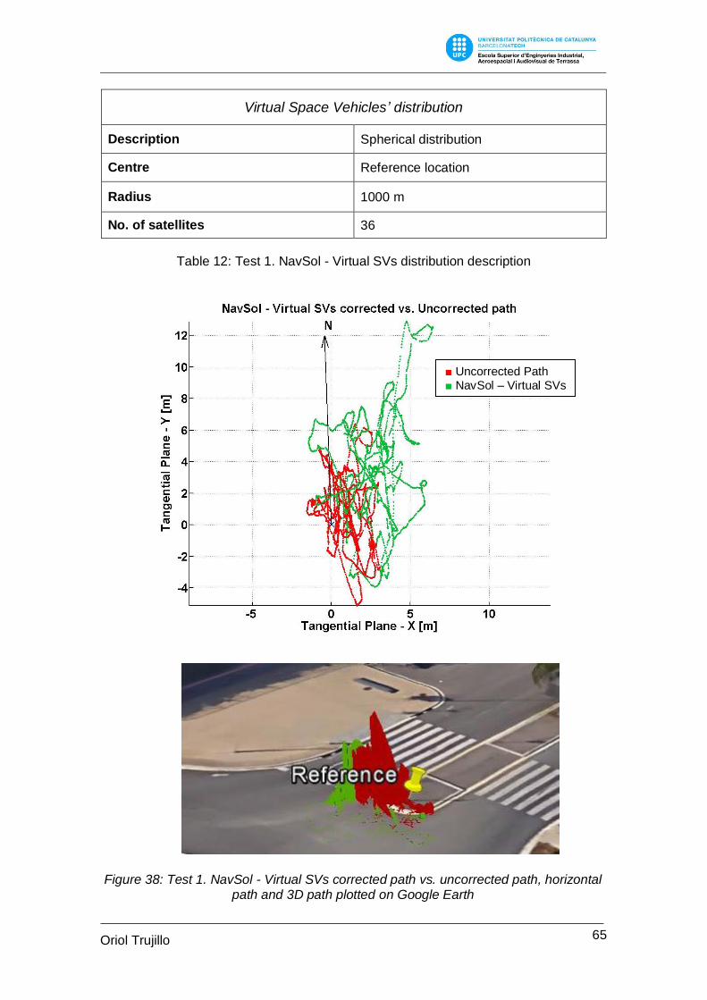
65 Oriol Trujillo
Martí
Virtual Space Vehicles’ distribution
Description Spherical distribution
Centre Reference location
Radius 1000 m
No. of satellites 36
Table 12: Test 1. NavSol - Virtual SVs distribution description
Uncorrected Path NavSol – Virtual SVs
Uncorrected Path Common DGPS
Figure 38: Test 1. NavSol - Virtual SVs corrected path vs. uncorrected path, horizontal
path and 3D path plotted on Google Earth
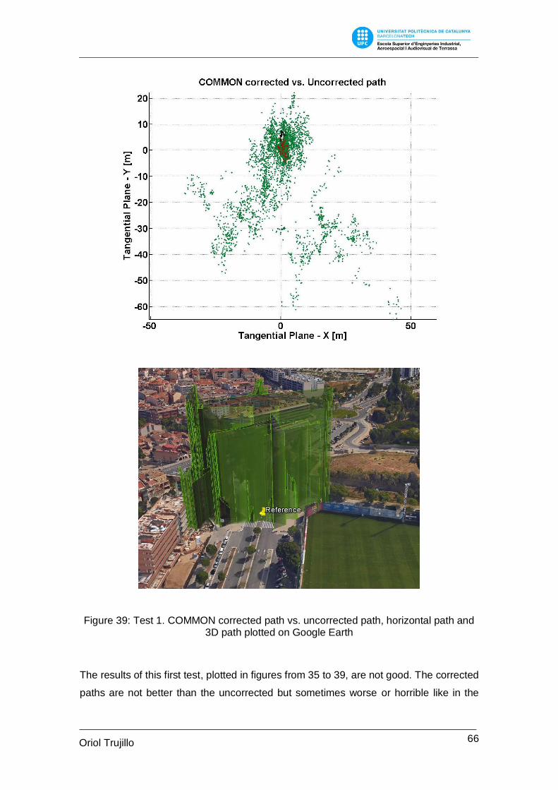
66 Oriol Trujillo
Martí
Figure 39: Test 1. COMMON corrected path vs. uncorrected path, horizontal path and
3D path plotted on Google Earth
The results of this first test, plotted in figures from 35 to 39, are not good. The corrected
paths are not better than the uncorrected but sometimes worse or horrible like in the
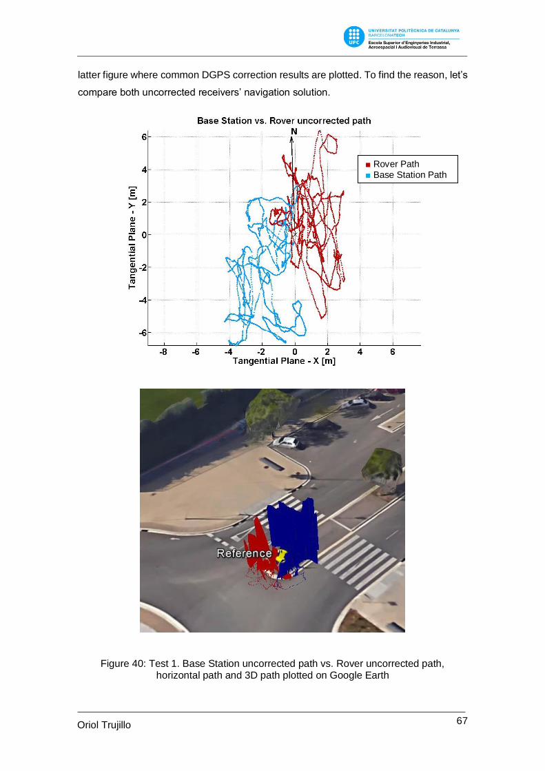
67 Oriol Trujillo
Martí
latter figure where common DGPS correction results are plotted. To find the reason, let’s
compare both uncorrected receivers’ navigation solution.
Figure 40: Test 1. Base Station uncorrected path vs. Rover uncorrected path,
horizontal path and 3D path plotted on Google Earth
Rover Path Base Station Path
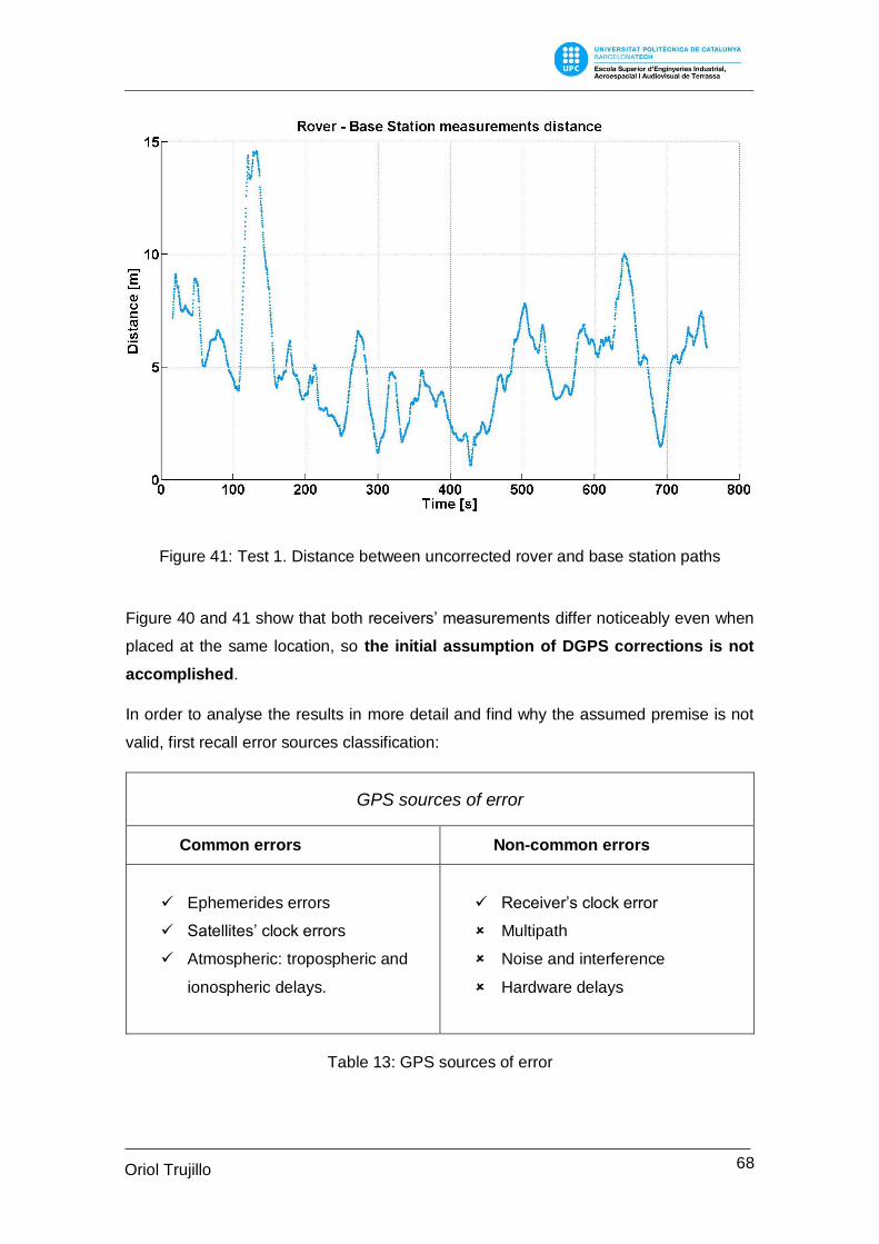
68 Oriol Trujillo
Martí
Figure 41: Test 1. Distance between uncorrected rover and base station paths
Figure 40 and 41 show that both receivers’ measurements differ noticeably even when
placed at the same location, so the initial assumption of DGPS corrections is not
accomplished.
In order to analyse the results in more detail and find why the assumed premise is not
valid, first recall error sources classification:
GPS sources of error
Common errors Non-common errors
Ephemerides errors
Satellites’ clock errors
Atmospheric: tropospheric and
ionospheric delays.
Receiver’s clock error
Multipath
Noise and interference
Hardware delays
Table 13: GPS sources of error
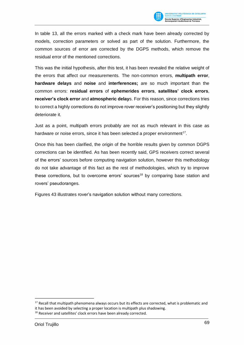
69 Oriol Trujillo
Martí
In table 13, all the errors marked with a check mark have been already corrected by
models, correction parameters or solved as part of the solution. Furthermore, the
common sources of error are corrected by the DGPS methods, which remove the
residual error of the mentioned corrections.
This was the initial hypothesis, after this test, it has been revealed the relative weight of
the errors that affect our measurements. The non-common errors, multipath error,
hardware delays and noise and interferences; are so much important than the
common errors: residual errors of ephemerides errors, satellites’ clock errors,
receiver’s clock error and atmospheric delays. For this reason, since corrections tries
to correct a highly corrections do not improve rover receiver’s positioning but they slightly
deteriorate it.
Just as a point, multipath errors probably are not as much relevant in this case as
hardware or noise errors, since it has been selected a proper environment17.
Once this has been clarified, the origin of the horrible results given by common DGPS
corrections can be identified. As has been recently said, GPS receivers correct several
of the errors’ sources before computing navigation solution, however this methodology
do not take advantage of this fact as the rest of methodologies, which try to improve
these corrections, but to overcome errors’ sources18 by comparing base station and
rovers’ pseudoranges.
Figures 43 illustrates rover’s navigation solution without many corrections.
17 Recall that multipath phenomena always occurs but its effects are corrected, what is problematic and it has been avoided by selecting a proper location is multipath plus shadowing. 18 Receiver and satellites’ clock errors have been already corrected.
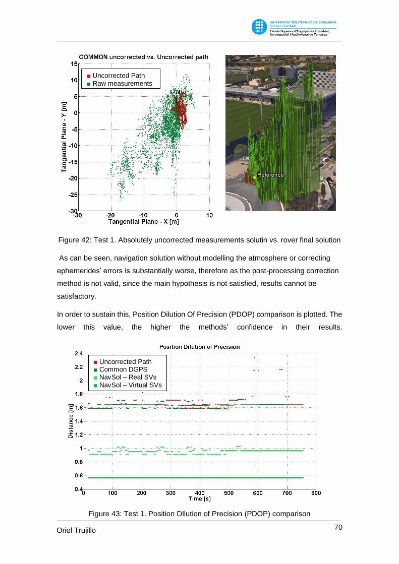
70 Oriol Trujillo
Martí
Figure 42: Test 1. Absolutely uncorrected measurements solutin vs. rover final solution
As can be seen, navigation solution without modelling the atmosphere or correcting
ephemerides’ errors is substantially worse, therefore as the post-processing correction
method is not valid, since the main hypothesis is not satisfied, results cannot be
satisfactory.
In order to sustain this, Position Dilution Of Precision (PDOP) comparison is plotted. The
lower this value, the higher the methods’ confidence in their results.
Uncorrected Path Raw measurements
Uncorrected Path Common DGPS NavSol – Real SVs NavSol – Virtual SVs
Figure 43: Test 1. Position DIlution of Precision (PDOP) comparison
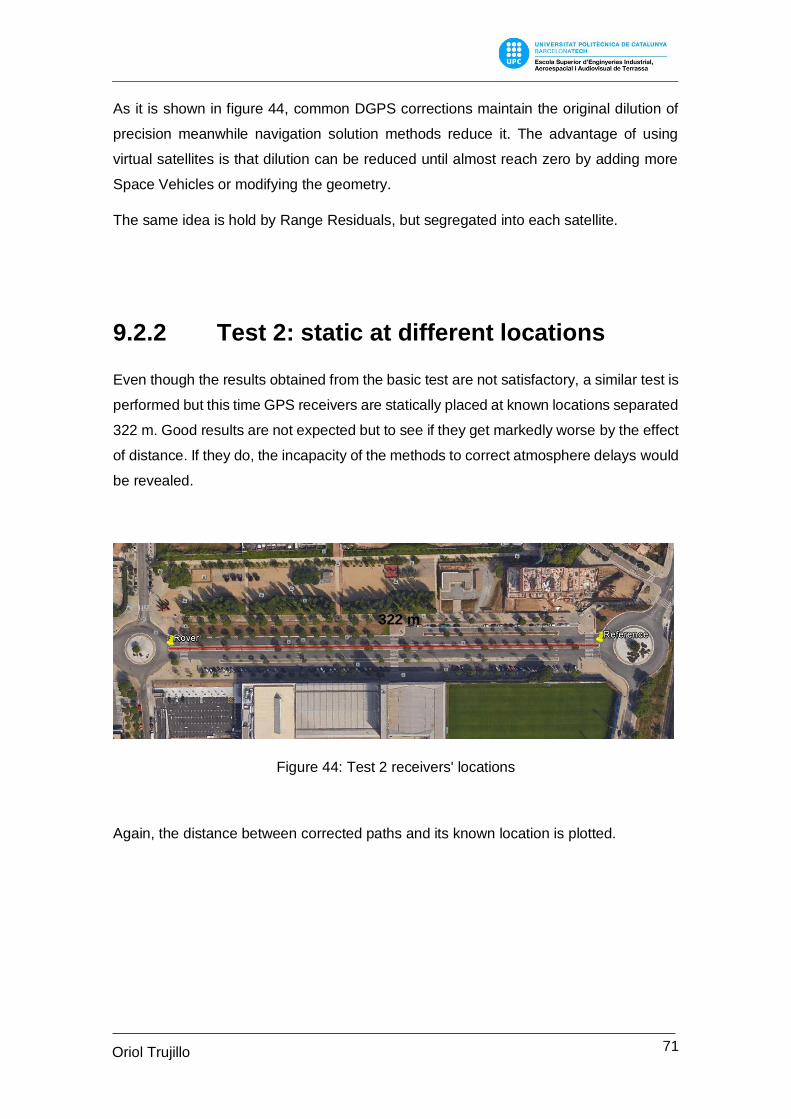
71 Oriol Trujillo
Martí
As it is shown in figure 44, common DGPS corrections maintain the original dilution of
precision meanwhile navigation solution methods reduce it. The advantage of using
virtual satellites is that dilution can be reduced until almost reach zero by adding more
Space Vehicles or modifying the geometry.
The same idea is hold by Range Residuals, but segregated into each satellite.
9.2.2 Test 2: static at different locations
Even though the results obtained from the basic test are not satisfactory, a similar test is
performed but this time GPS receivers are statically placed at known locations separated
322 m. Good results are not expected but to see if they get markedly worse by the effect
of distance. If they do, the incapacity of the methods to correct atmosphere delays would
be revealed.
Figure 44: Test 2 receivers' locations
Again, the distance between corrected paths and its known location is plotted.
322 m
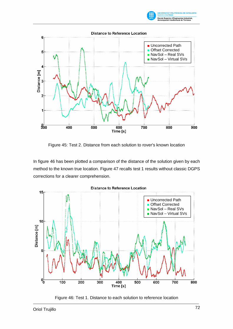
72 Oriol Trujillo
Martí
Figure 45: Test 2. Distance from each solution to rover's known location
In figure 46 has been plotted a comparison of the distance of the solution given by each
method to the known true location. Figure 47 recalls test 1 results without classic DGPS
corrections for a clearer comprehension.
Figure 46: Test 1. Distance to each solution to reference location
Uncorrected Path Offset Corrected NavSol – Real SVs NavSol – Virtual SVs
Uncorrected Path Offset Corrected NavSol – Real SVs NavSol – Virtual SVs
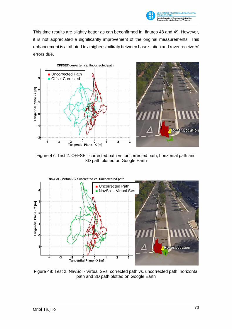
73 Oriol Trujillo
Martí
This time results are slightly better as can beconfirmed in figures 48 and 49. However,
it is not appreciated a significantly improvement of the original measurements. This
enhancement is attributed to a higher similiraty between base station and rover receivers’
errors due.
Figure 47: Test 2. OFFSET corrected path vs. uncorrected path, horizontal path and 3D path plotted on Google Earth
Figure 48: Test 2. NavSol - Virtual SVs corrected path vs. uncorrected path, horizontal path and 3D path plotted on Google Earth
Uncorrected Path Offset Corrected
Uncorrected Path NavSol – Virtual SVs

74 Oriol Trujillo
Martí
Nonetheless, it has to be note that altitude is highly corrected. Since it is the hardest
coordinate to estimate, due to the poor satellite spreading along this coordinate (most of
the Space Vehicles are eclipsed by the Earth), GPS receivers tend to calculate a higher
altitude than the real value, giving to the correction methods a chance to improve
positioning.
75 Oriol Trujillo
Martí
10. Environmental Impact
The direct environmental impact of the implementation of this project almost zero,
since no CO2 emissions have been produced and the only power consumption has been
the basic to supply energy to the computer.
As the majority of the applications, it has an indirect environmental impact associated
and several factors has to be considered. In this case, it must be accounted that pollution
is emitted when the devices (PC, Pixhawk, GPS receivers and cables) are transported
from the manufacturer to the buyer, as well the contamination produced in the fabrication
process and the fact that, the electronic components are not easy to be discomposed by
the nature if they are improperly discarded. Luckily, it is in our hands to avoid that.
Once the methodology presented in this projected could be applied to real UAVs
applications, it would also be associated to the power consumption required to fly, which
would be usually electric.
However, it has also a positive effect, such as this affordable GPS enhancement allows
to improve the performance of a lot of civil applications based on UAVs most of them
focused on avoiding forest fires, high-precision agriculture, control and protection of the
fauna, and more of them that involve the conservation of the environment.

76 Oriol Trujillo
Martí
11. Future planning and scheduling
In this section it is proposed a planning and scheduling for the future lines of investigation
that precede this study.
In order to achieve a centimetre-level precision, as specified in the requirements, it is
necessary the upgrade the receivers to a dual-frequency (L1 and L2) capable receivers,
using carrier-phase measurements and applying radio interferometry technique. Also
GPS receivers should be able to output raw data.
Once this is accomplished, it might be studied the possibility of implementing a real-time
application.
These goals are split in the tasks described below, which have been scheduled between
the time lapse going from 1st September 2016 to 31st January 2017.
1. Purchase of new GPS receivers: extensive research of the market possibilities and
acquire the best option considering the demanded specifications and the limited
resources.
2. Adapt code the new receivers: the implemented code needs to be updated
considering new receivers.
2.1. Decode new messages: decode new according to the protocols.
2.2. Modify to work with carrier-phase measurements: adapt the program to work with
carrier-phase measurements.
2.3. Validate the code: as in the present study, the code is extensively validated to ensure
that it is free of errors.
2.4. Test the resulting program: the resulting validated program has to be tested.
3. Analyse of the results: analyse and compare new precision, Dilution Of Precision
and so on.
4. Implement methodology in real-time: implement the correction methodology as
a real-time corrections.
77 Oriol Trujillo
Martí
4.1. Select and purchase communication link: study the necessities and the
market offer in order to choose the best components for the current purpose.
Then buy them.
4.2. Optimize the code: optimize to reduce the computational cost and speed
up the methodology.
4.3. Select and acquire rover’s microprocessor: it is necessary in order to
apply DGPS corrections and compute position an auxiliary microprocessor
with enough computational power.

77 Oriol Trujillo
Martí
11.1 Proposed schedule for future work
Name of the task Work September Octuber November December January
Purchase of the new GPS receivers 15d
Adapt code to new receivers 54d
Decode new messages 10d
Modify to work with carrier-phase measurements
30d
Validate the code 30d
Test the resulting program 10d
Analyse the results 15d
Implement methodology in real-time 50d
Select and purchase communication link 30d
Optimize the code 20d
Select and acquire rover's microprocessor 30d
Validate real-time application 20d
78 Oriol Trujillo
Martí
12. Conclusions
It is clear that the main goal of the project has not been reached, since a reliable post-
processing correction methodology is not achieved, or at least none of them could be
validated for the set conditions.
However, the origin of the problem has been identified. Tests have failed because the
initial hypothesis of Differential GPS corrections is not satisfied, since both receivers’
errors differ more than expected even when placed at the reference location. This is due
to atmospheric residual errors are lower and receiver electronics’ errors higher, for the
available receivers, than we had anticipated.
Furthermore, it has been implemented a program that works as a good environment for
dealing with GPS data. Allowing the user to monitor and work with data, since a bunch
of post-processing functions are given and user’s implemented functions can be easily
incorporated. Also, navigation solution computation is externalised and can be
performed on the computer, enabling the possibility to introduce any desired modification
such as changing position’s computation process, atmospheric models, adding
corrections, etc.
Additionally, the code is able to overcome the problem of the disabled raw data by
estimating pseudoranges and computing satellites’ paths. Obviously, it is also ready to
apply DGPS corrections when a suitable scenario is given.
The other requirement, referred to the cost of the whole project, it has been clearly
satisfied. The total budget ascends to 27407.22€ (see BUDGET document) accounting
the personnel cost, but considering giving the software as free-license, a user that
already owns a computer with MATLAB and a UAV using Pixhawk, which is for instance
the case of the Aerospace Department of ESEIAAT (UPC), could implement these
system for 224.61€ including both GPS receivers. Which it is far from the thousands of
euros that costs a professional equipment.

79 Oriol Trujillo
Martí
Finally, just remark that it has been a continuous learning process full of difficulties that
have been overcome, such as to communicate with receivers, decode input messages,
estimate disabled raw data and a lot of unexpected troubles; and even a correction
method has been proposed.
That is why, despite of the unsuccessful results, I can feel proud of the job done.

80 Oriol Trujillo
Martí
13. Bibliography
[1] Trimble Navigation. GPS diferencial explicado claramente.1993
[2] Christopher, and Elliot Kaplan. Understanding GPS. Principles and Applications.
Norwood: Artech House, 2006.
[3] Doberstein, Dan. Fundamentals of GPS Receivers. A hardware approach.
NewYork: Springer, 2012.
[4] Dennis, Nicolaj, Peter, Søren, and Kai Borre. A software-defined GPS and Galileo
receiver. A single-frequency approach. Boston: Birkhäuser, 2007.
[5] El-Rabbany, Ahmed. Introduction to GPS. The Global Positioning System.
Norwood: Artech House, 2002.
[6] 3D Robotics Store – 3DR uBlox GPS with Compass Kit.
https://store.3dr.com/products/3dr-gps-ublox-with-compass, February 2016.
[7] NEO-7 Series Product Summary. u-blox 7 GNSS modules. https://www.u-
blox.com/sites/default/files/products/documents/NEO-7_ProductSummary_(UBX-
13003342).pdf, February 2016.
[8] NEO-7 – u-blox GNSS 7 modules – Data Sheet. https://www.u-
blox.com/sites/default/files/products/documents/NEO-7_DataSheet_(UBX-
13003830).pdf, February 2016.
[9] Wiki Open Street Map – UbloxRaw. http://wiki.openstreetmap.org/wiki/RTKLIB,
March 2016.
[10] GPS Information – Almanac an Ephemeris Data as used by GPS receivers.
http://gpsinformation.net/main/almanac.txt, March 2016.
[11] ManualZZ – Affordable Differential GPS – Australian National University.
http://manualzz.com/doc/10599074/affordable-differential-gps, March2015¡6.
[12] Swift Navigation – Piksi. https://www.swiftnav.com/piksi.html, March 2016.
81 Oriol Trujillo
Martí
[13] Wiki Open Street Map – RTKlib, http://wiki.openstreetmap.org/wiki/RTKLIB, March
2016.
[14] ESA Navipedia - RTK Standards – RTCM Standards.
http://www.navipedia.net/index.php/RTK_Standards, March 2016.
[15] The Radio Technical Comision for Maritime Services – RTCM Standards.
http://www.rtcm.org/overview.php, March 2016.
[16] GPS Information – NMEA Data. http://www.gpsinformation.org/dale/nmea.htm,
March 2016.
[17] Global Positioning System directorate – Systems Engineering & Integration –
Interface Specification – IS-GPS-200H. http://www.gps.gov/technical/icwg/IS-
GPS-200H.pdf, April 2016.
[18] Global Positioning System directorate – Systems Engineering & Integration –
Interface Specification – IS-GPS-200G. http://www.gps.gov/technical/icwg/IS-
GPS-200G.pdf, April 2016.
[19] u-blox 7 Receiver Description – Including Protocol Specification V14.
https://www.u-blox.com/sites/default/files/products/documents/u-blox7-
V14_ReceiverDescrProtSpec_(GPS.G7-SW-12001)_Public.pdf, May 2016.
[20] Taoglass - 2mm thick GPS Patch Antenna, 1575MHz. http://www.taoglas.com/wp-
content/uploads/2015/04/GP.1575.18.2.A.02.pdf, June 2016.
[21] MathWorks – Pricing and Licensing. http://es.mathworks.com/pricing-
licensing/?prodcode=ML, 19/06/2016.