study of iron ion transit through three-fold channel of

BearWorks BearWorks

MSU Graduate Theses

Summer 2017

Study of Iron Ion Transit through Three-Fold Channel of Ferritin Study of Iron Ion Transit through Three-Fold Channel of Ferritin

Cage Cage

Shah Alam Limon Missouri State University, [email protected]

As with any intellectual project, the content and views expressed in this thesis may be

considered objectionable by some readers. However, this student-scholar’s work has been

judged to have academic value by the student’s thesis committee members trained in the

discipline. The content and views expressed in this thesis are those of the student-scholar and

are not endorsed by Missouri State University, its Graduate College, or its employees.

Follow this and additional works at: https://bearworks.missouristate.edu/theses

Part of the Biology and Biomimetic Materials Commons, and the Biomaterials Commons

Recommended Citation Recommended Citation Limon, Shah Alam, "Study of Iron Ion Transit through Three-Fold Channel of Ferritin Cage" (2017). MSU Graduate Theses. 3123. https://bearworks.missouristate.edu/theses/3123

This article or document was made available through BearWorks, the institutional repository of Missouri State University. The work contained in it may be protected by copyright and require permission of the copyright holder for reuse or redistribution. For more information, please contact [email protected].

https://bearworks.missouristate.edu/

https://bearworks.missouristate.edu/theses

https://bearworks.missouristate.edu/theses?utm_source=bearworks.missouristate.edu%2Ftheses%2F3123&utm_medium=PDF&utm_campaign=PDFCoverPages

http://network.bepress.com/hgg/discipline/286?utm_source=bearworks.missouristate.edu%2Ftheses%2F3123&utm_medium=PDF&utm_campaign=PDFCoverPages

http://network.bepress.com/hgg/discipline/233?utm_source=bearworks.missouristate.edu%2Ftheses%2F3123&utm_medium=PDF&utm_campaign=PDFCoverPages

https://bearworks.missouristate.edu/theses/3123?utm_source=bearworks.missouristate.edu%2Ftheses%2F3123&utm_medium=PDF&utm_campaign=PDFCoverPages

mailto:[email protected]

STUDY OF IRON ION TRANSIT THROUGH THREE-FOLD

CHANNEL OF FERRITIN CAGE

A Masters Thesis

Presented to

The Graduate College of

Missouri State University

TEMPLATE

In Partial Fulfillment

Of the Requirements for the Degree

Master of Science, Materials Science

By

Shah Alam Limon

August 2017

ii

Copyright 2017 by Shah Alam Limon

iii

STUDY OF IRON ION TRANSIT THROUGH THREE-FOLD CHANNEL OF

FERRITIN CAGE

Physics, Astronomy and Materials Science

Missouri State University, August 2017

Master of Science

Shah Alam Limon

ABSTRACT

Ferritin is an iron-storage globular protein with an ability to uptake, mineralize and

release iron ions in a controllable manner. The globular hollow shell allows storage of

mineralized iron, with several channels responsible for the transit of ions into the shell

and out of it. Understanding of the detailed molecular functioning of ferritin is required

for rational design of biomimetic conjugate nano-biosystems containing ferritin-like

constituents. In this work, ferritin was investigated both numerically by all-atom

molecular dynamics (MD) simulations, and experimentally by Raman spectroscopy.

Molecular dynamic simulations of a model system comprising iron ions (Fe2+) and a

ferritin trimer expressing a three-fold channel responsible for the ion transport, have

revealed a quick entering of ions in the channel. The transit of iron ions through the

channel was thoroughly investigated. The transit was found to be driven by both

electrostatic charge of ferritin, and interaction between the ions. Exit (expulsion) of an

iron ion from the channel was observed at a condition that at least one more ion is present

in the channel. Raman characterization of an iron-loaded ferritin solution revealed

pronounced bands attributable to iron, as expected. However, Raman spectra of apo-

ferritin, which does not contain an iron mineral, also exhibited similar bands. Based on

the results of MD simulations, it was hypothesized that apo-ferritin retains iron ions in its

three-fold channels, and these ions may produce the observed Raman bands. The study of

molecular mechanisms involved in the iron ion transit elucidates the pathways of iron

uptake and release in ferritin.

KEYWORDS: ferritin, iron ion transit, molecular dynamics, Raman spectroscopy,

nano-biological conjugation

This abstract is approved as to form and content

_______________________________

Maria Stepanova, PhD

Chairperson, Advisory Committee

Missouri State University

iv

STUDY OF IRON ION TRANSIT THROUGH THREE-FOLD

CHANNEL OF FERRITIN CAGE

By

Shah Alam Limon

A Masters Thesis

Submitted to the Graduate College

Of Missouri State University

In Partial Fulfillment of the Requirements

For the Degree of Master of Science, Materials Science

August 2017

Approved:

_______________________________________

Maria Stepanova, PhD

_______________________________________

Kartik Ghosh, PhD

_______________________________________

Matthew Siebert, PhD

_______________________________________

Julie Masterson, PhD: Dean, Graduate College

In the interest of academic freedom and the principle of free speech, approval of this thesis indicates the

format is acceptable and meets the academic criteria for the discipline as determined by the faculty that

constitute the thesis committee. The content and views expressed in this thesis are those of the student-

scholar and are not endorsed by Missouri State University, its Graduate College, or its employees.

v

ACKNOWLEDGEMENTS

I am very thankful to the Department of Physics, Astronomy and Materials

Science of Missouri State University for providing enormous facilities to complete my

graduate studies here. I am thankful to my research supervisor Dr. Maria Stepanova for

continuously helping me learn about experimental and molecular dynamics simulation

techniques. Special thanks to my academic advisor and thesis committee member Dr.

Kartik Ghosh, who inspired me in achieving success, helped me in academic affairs and

guided me in the right direction whenever needed. I am grateful to Dr. Matthew Siebert,

for being the thesis committee member. I also want to thank Dr. Mayanovic, Dr.

Plavchan and Dr. Sakidja for allowing me to use different experimental and

computational resources.

As an international student here at MSU, it has been a great privilege for me to

have wonderful host families: Nancy & Kent Parrish, Twyla & Bob McGurty, Susan &

Mike Burton, and Suzanne & Ted Lennard. I am thankful to them for sharing American

culture with me and making my time here in Springfield, MO very much fantastic.

Fellow graduate students Delower, Harsha, Shaolin, Paul, Bithi, Reaz, Samiul, Austin,

and Dan helped me in my research work in different ways, and I am grateful to them.

Last but not least, I am thanking my parents, Dr. Liakat Ali and Ms. Dalia Shirin,

my sister Shabnam, and my wife Anahita for supporting me always.

vi

TABLE OF CONTENTS

CHAPTER 1: Introduction ..................................................................................................1

CHAPTER 2: Literature Review .........................................................................................2

2.1. Biotic And Abiotic Nanomaterials....................................................................2

2.2 Raman And Surface Enhanced Raman Spectroscopy .......................................3

2.3 Sers Of Biological Samples ...............................................................................7

2.4 Molecular Dynamics Simulations ....................................................................10

2.5. Ferritin And Other Cage Proteins ...................................................................13

2.6. Goals And Objectives Of The Work ...............................................................17

CHAPTER 3: Experimental Methods ................................................................................19

3.1. LabRAM HR 800 Evolution Raman Spectroscope ........................................19

3.2. Sample Preparation .........................................................................................21

3.3. Acquisition Of Raman Spectra .......................................................................25

CHAPTER 4: Computational Methods .............................................................................26

4.1. The GROMACS Molecular Simulation Package ...........................................26

4.2. Preparation Of Model For Simulation ............................................................28

4.3. Energy Minimization ......................................................................................30

4.4. Equilibration ...................................................................................................32

4.5. Production MD Simulations ...........................................................................34

4.6. Visualization And Analysis Softwares ...........................................................35

CHAPTER 5: Computational Results ................................................................................38

5.1. Transport Of Fe Ions Through Ferritin’s Channel ..........................................38

5.2. Electrostatic potential around ferritin’s channel .............................................46

5.3. Coordination Of Fe Ions In The Channel .......................................................48

CHAPTER 6: Experimental Results ..................................................................................53

6.1. Raman Spectra Of Ferritin ..............................................................................53

6.2. Raman Characterization Of Mohr’s Salt .........................................................59

6.3. Tentative SERS Characterization Of Ferritin .................................................61

CHAPTER 7: Discussion ...................................................................................................65

CHAPTER 8: Conclusions And Future Work ...................................................................67

8.1. Conclusions .....................................................................................................67

8.2. Future Work ....................................................................................................68

REFERENCES ..................................................................................................................70

vii

LIST OF TABLES

Table 4.1: Visualization and analysis software for MD analysis...................................... 37

Table 5.1: Sets of production MD simulations. ................................................................ 41

Table 6.1: Hypothetical Raman band assignments of ferritin solution (from Refs. 16, 108-

116) ................................................................................................................................... 54

viii

LIST OF FIGURES

Figure 2.1: Raman scattering types. Adapted with permission from Ref. 10. .................... 4

Figure 2.2: Energy level diagram for Raman and Rayleigh scattering. .............................. 5

Figure 2.3: Scheme of Localized Surface Plasmon Resonance excitation by incident

monochromatic light. Reproduced with permission from Ref. 13...................................... 7

Figure 2.4: Ferritin monomer, PDB ID 5CZU.63 The mage was generated using

PYMOL64. ......................................................................................................................... 14

Figure 2.5: Ferrihydrite mineral inside ferritin cage and SEM image of iron loaded

ferritin. Reproduced with permission from Ref. 66. .......................................................... 15

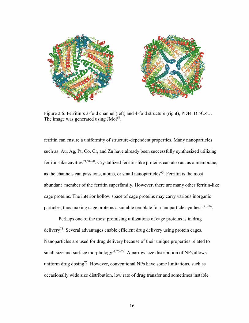
Figure 2.6: Ferritin’s 3-fold channel (left) and 4-fold structure (right), PDB ID 5CZU.

The image was generated using JMol67. ........................................................................... 16

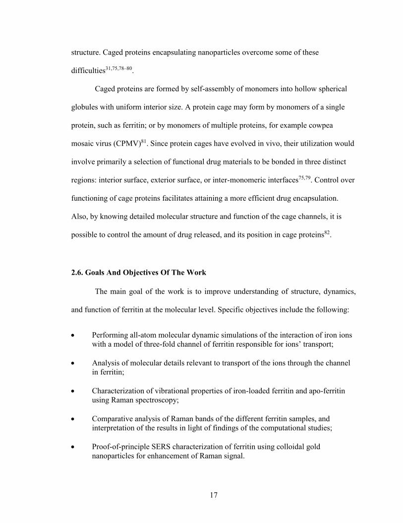
Figure 2. 7: Nanodot synthesis using ferritin as a template. Reproduced with permission

from Ref. 65 . ..................................................................................................................... 18

Figure 3.1: Horiba LabRAM HR 800 Evolution Raman spectrometer.20

Figure 3. 2: Schematic diagram of Raman spectroscope. ................................................. 20

Figure 3.3: Samples of (A) liquid ferritin, (B) solid powdered ferritin, and (C) Mohr’s

salt. .................................................................................................................................... 22

Figure 3.4: 80 nm Au nanoparticles in PBS solution, and SEM image of the deposited Au

NPs on PBS solution on a 10 nm Au coated glass substrate. ........................................... 23

Figure 3.5: Experimental setup for liquid sample Raman characterization. ..................... 23

Figure 3.6: Raman spectroscopy setup showing incident laser on sample on a substrate. 24

Figure 3.7: Incubation setup and cross-sectional schematic of a Petri dish with a sample.

........................................................................................................................................... 24

Figure 4.1: PyMOL generated 3-fold ferritin structure.29

Figure 4.2: Process flow chart of molecular dynamics simulation. .................................. 33

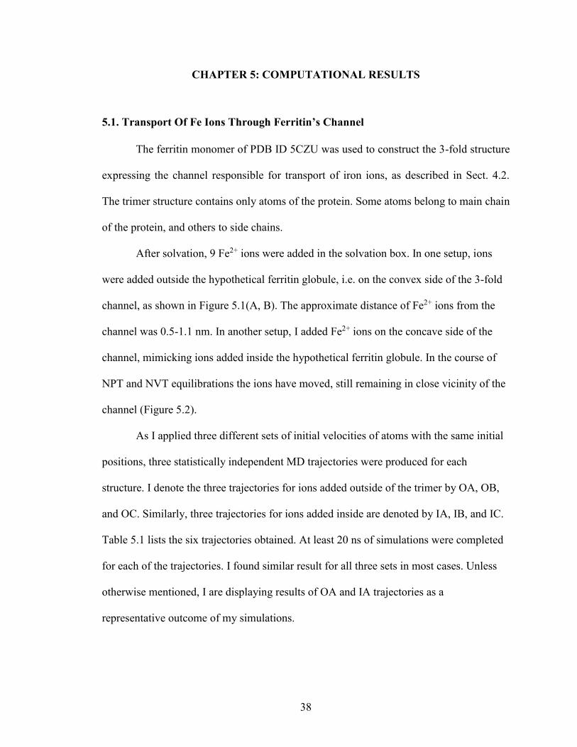
Figure 5.1: Initial structures of ferritin’s trimer with nine iron ions before equilibration:

A) Fe2+ ions added outside of the ferritin trimer, B) side view of ions outside the trimer,

C) Fe2+ ions added inside of the ferritin trimer, D) side view of ions inside the trimer.

Iron ions are shown with red spheres………………………….…………………………39

ix

Figure 5.2: Iron ion positions after equilibration: A) ions added outside of the trimer, B)

ions added outside side view, C) ions added inside of the trimer, D) ions added inside

side view. Ions are shown by red spheres. ........................................................................ 40

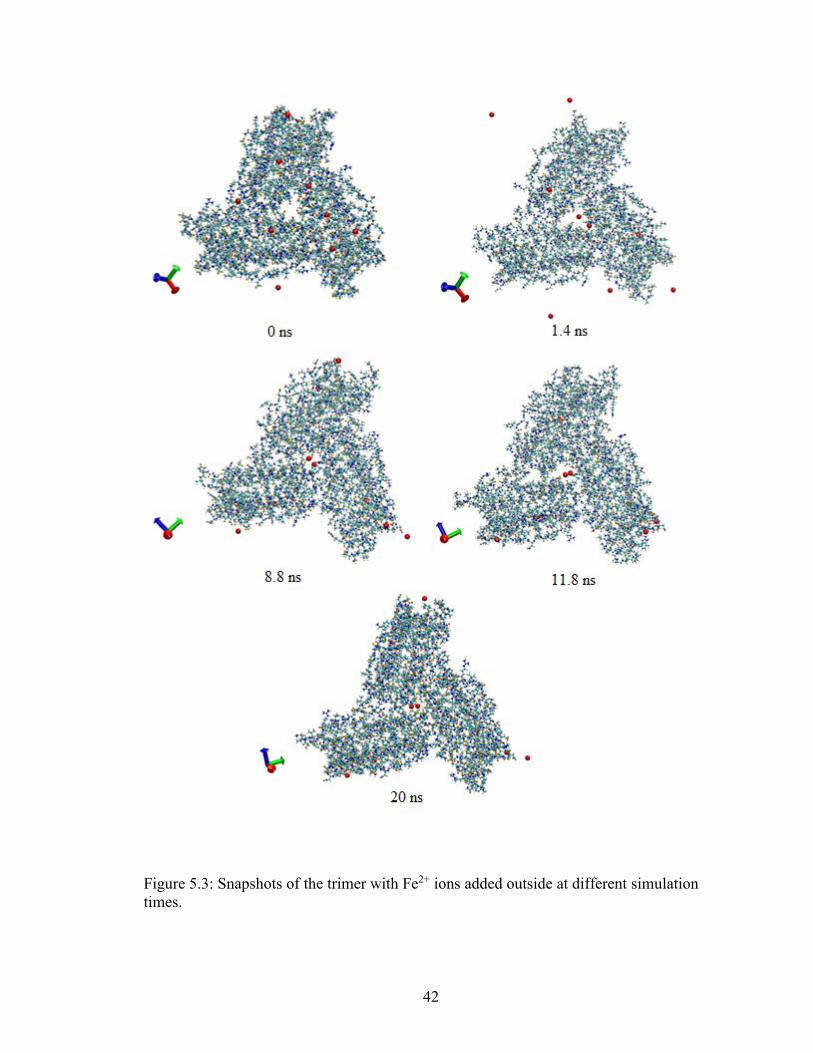
Figure 5.3: Snapshots of the trimer with Fe2+ ions added outside at different simulation

times. ................................................................................................................................. 42

Figure 5.4: Snapshots of the trimer with Fe2+ ions added inside. Ions are shown with red

spheres............................................................................................................................... 43

Figure 5.5: RMSD plot of the first ion that entered the channel from outside, as illustrated

in figure 5.3. ...................................................................................................................... 44

Figure 5.6: RMSD plot of the first ion that entered the channel from inside, as illustrated

in figure 5.4. ...................................................................................................................... 45

Figure 5.7: Electrostatic potential, color-coded and mapped onto the solvent-accessible

surface of ferritin trimer after equilibration (left), and when at least one iron ion entered

the channel (right). The ions are shown as yellow spheres. Two panels on the top show

outer surface of the trimer, and those on the bottom show inner surface. ........................ 46

Figure 5.8: Iron ion (red sphere) surrounded by carboxylate group of Glu130 residue in

the 3-fold channel of ferritin. ............................................................................................ 48

Figure 5.9: Close-up of Glu130 residues of three chains of ferritin and water solvation

shell surrounding a Fe2+ ion in the channel of ferritin. ..................................................... 48

Figure 5.10: Solvent Accessible Surface (SAS) of ferritin’s channel with Fe2+ ion in the

channel at 1.4 ns (A), and the ion exiting the channel while second ion approaching at

s11.8 ns of the simulation for ions added outside of the trimer. ....................................... 49

Figure 5.11: RDF of iron ion entering the channel from outside...................................... 51

Figure 5.12: RDF of iron ion entering the channel from inside........................................ 52

Figure 6.1: Baseline subtracted Raman spectrum of ferritin on Si substrate.……………53

Figure 6.2: Raman spectrum of powder apo-ferritin on Si substrate. ............................... 56

Figure 6.3: Raman spectra of powered apo-ferritin in water after incubation. No filter was

used during laser excitation, and water evaporated from the sample. .............................. 57

Figure 6.4: Raman spectra of powered apo-ferritin in water after incubation. A 50% filter

was used during laser excitation, and water did not evaporate. ........................................ 58

Figure 6.5: Raman spectra of Mohr’s salt on Si substrate. ............................................... 60

Figure 6.6: Raman spectrum of Mohr salt incubated in HPLC DI water on Si substrate. 60

x

Figure 6.7: Raman spectrum of citrate-stabilized Au nanoparticles’ solution on a Si

substrate. ........................................................................................................................... 62

Figure 6.8: Raw Raman spectra of ferritin solution with Au nanoparticles (red line), and

of regular ferritin solution without nanoparticles (blue line) on Au coated glass substrate.

These spectra were not background-subtracted. ............................................................... 63

Figure 6.9: Background-subtracted Raman spectrum of ferritin solution containing Au

nanoparticles. .................................................................................................................... 64

1

CHAPTER 1: INTRODUCTION

The work described here is dedicated to computational and experimental studies

of ferritin, a cage protein involved in iron ion storage and release processes. Applications

of ferritin include rational design of biomimetic conjugate nano-biosystems, synthesizing

nanodot arrays, protein crystallization to form nano-porous membranes, transport of drug

delivery agents, and many others.

In this work, all-atom molecular dynamics simulations of a fragment of ferritin

cage are done in order to better understand detailed functioning of ferritin. The fragment

considered expresses a three-fold channel, which is responsible for transport of iron ions

in and out of ferritin globule. The molecular dynamics procedures, including energy

minimization, equilibration, and production simulations were done using the GROMACS

molecular dynamics package. Transit of iron ions through the three-fold channel was

thoroughly analyzed.

In experimental studies of ferritin, Raman spectroscopy was used. The advantage

of Raman spectroscopy is that it allows capturing unique vibrational fingerprints of

molecules. In this work, Raman spectra of iron-loaded ferritin solution were collected.

Raman spectra of apo-ferritin were also acquired. Colloidal Au nanoparticles were

employed in one of the experimental setups in order to achieve surface enhanced Raman

scattering of ferritin samples. Results of Raman characterization of the various samples

of ferritin were interpreted in light of molecular mechanisms revealed by the

computational studies.

2

CHAPTER 2: LITERATURE REVIEW

2.1. Biotic and Abiotic Nanomaterials

Conventionally the term “nano” is attributed to an object of 100 nm dimensions or

below. Nevertheless, FDA and IUPAC suggest that any particle under one micrometer

with dimension-dependent property could be identified as a nanoparticle.1 The

conjugation of abiotic nanostructures with nanostructured biological species has

significant applications in various areas including drug delivery systems, bioimaging,

nanofabrication, bioenergy and biofuels, medicine, and biomimetic conjugate nano-bio

systems. The key aspect of both naturally occurring and processed biotic materials is their

biocompatibility inside living organisms. Abiotic nanostructures, in turn, act as a

constituent for characterization of biomolecules. For instance, Au and Ag nanoparticles

can greatly enhance the Raman scattering of biomolecules, a technique known as Surface

Enhanced Raman Spectroscopy (SERS) 2,3.

Nanoparticles can be found in nature or they can be synthesized artificially.

Natural nanoparticles are a result of natural phenomena, such as volcanic eruption or

forest fire 4,5. Synthesized nanoparticles can be prepared in different ways, such as

hydrothermal synthesis, gas condensation, chemical vapor deposition, dispersion in

solvent, synthesis by colloidal techniques, etc.6,7 Nucleation and growth processes play a

key role in nanoparticle synthesis6. Synthesized nanoparticles have tremendous

applications facilitated by their physical properties. One of the important applications is

detection of proteins and DNA5.

While discussing biotic- abiotic nanostructures, one of the most important criteria

would be size requirements. One of the aspects is size compatibility between

3

nanoparticles and biological species. To understand intra and inter cellular mechanisms,

which is important to interpret many functions of biological species, size compatibility

would be a significant factor. Average cell size of bio-organisms is approximately 10 μm.

The cell constituents are in a nm range; for instance, protein size is typically less than 100

nm. Incorporating nanoparticles of similar size as a probe is a promising technique to

understand cell mechanisms at a molecular level.

There is a wide range of applications for nanomaterials in biological sciences,

such as fluorescent tags for bio-detection, protein characterization, drug delivery, DNA

probing, enhancement of MRI contrast agents, or cancer cell detection.8 Besides the size

compatibility, interactions between nanoparticles and biomolecules are also important.

One interacting media is coating - for example, a biopolymeric coating that acts as

binding agent between biological and inorganic surfaces.

2.2 Raman and Surface Enhanced Raman Spectroscopy

Raman spectroscopy is a versatile non-destructive characterization technique

involving an extraordinary phenomenon called Raman scattering. It involves inelastic

scattering of photons from a molecule upon exposure to light. Raman spectra are

representative of vibrational characteristics of a material. Since Raman spectroscopy can

detect different modes of molecular vibrations, it shows unique vibrational fingerprints of

many materials including crystalline solids, non-crystalline solids, biological species,

liquids, thin films, etc. Raman effect was discovered by C.V. Raman in 1928, for which

he received his Nobel prize in 1930. Since then Raman spectroscopy is such a broadly

4

used characterization technique, that the Raman effect was granted the status of National

Historic Chemical Landmarks by American Chemical Society in 19989.

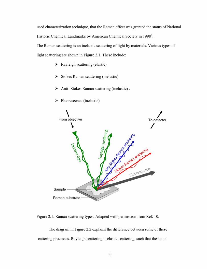
The Raman scattering is an inelastic scattering of light by materials. Various types of

light scattering are shown in Figure 2.1. These include:

➢ Rayleigh scattering (elastic)

➢ Stokes Raman scattering (inelastic)

➢ Anti- Stokes Raman scattering (inelastic) .

➢ Fluorescence (inelastic)

Figure 2.1: Raman scattering types. Adapted with permission from Ref. 10.

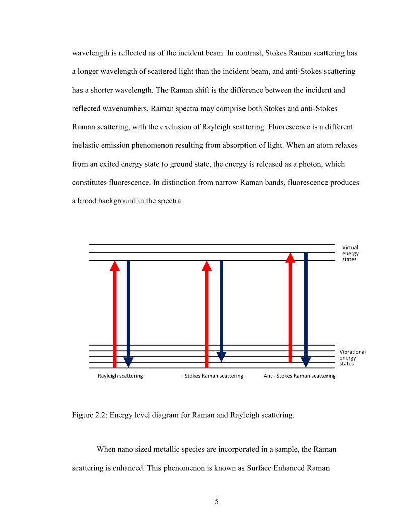
The diagram in Figure 2.2 explains the difference between some of these

scattering processes. Rayleigh scattering is elastic scattering, such that the same

5

wavelength is reflected as of the incident beam. In contrast, Stokes Raman scattering has

a longer wavelength of scattered light than the incident beam, and anti-Stokes scattering

has a shorter wavelength. The Raman shift is the difference between the incident and

reflected wavenumbers. Raman spectra may comprise both Stokes and anti-Stokes

Raman scattering, with the exclusion of Rayleigh scattering. Fluorescence is a different

inelastic emission phenomenon resulting from absorption of light. When an atom relaxes

from an exited energy state to ground state, the energy is released as a photon, which

constitutes fluorescence. In distinction from narrow Raman bands, fluorescence produces

a broad background in the spectra.

Figure 2.2: Energy level diagram for Raman and Rayleigh scattering.

When nano sized metallic species are incorporated in a sample, the Raman

scattering is enhanced. This phenomenon is known as Surface Enhanced Raman

6

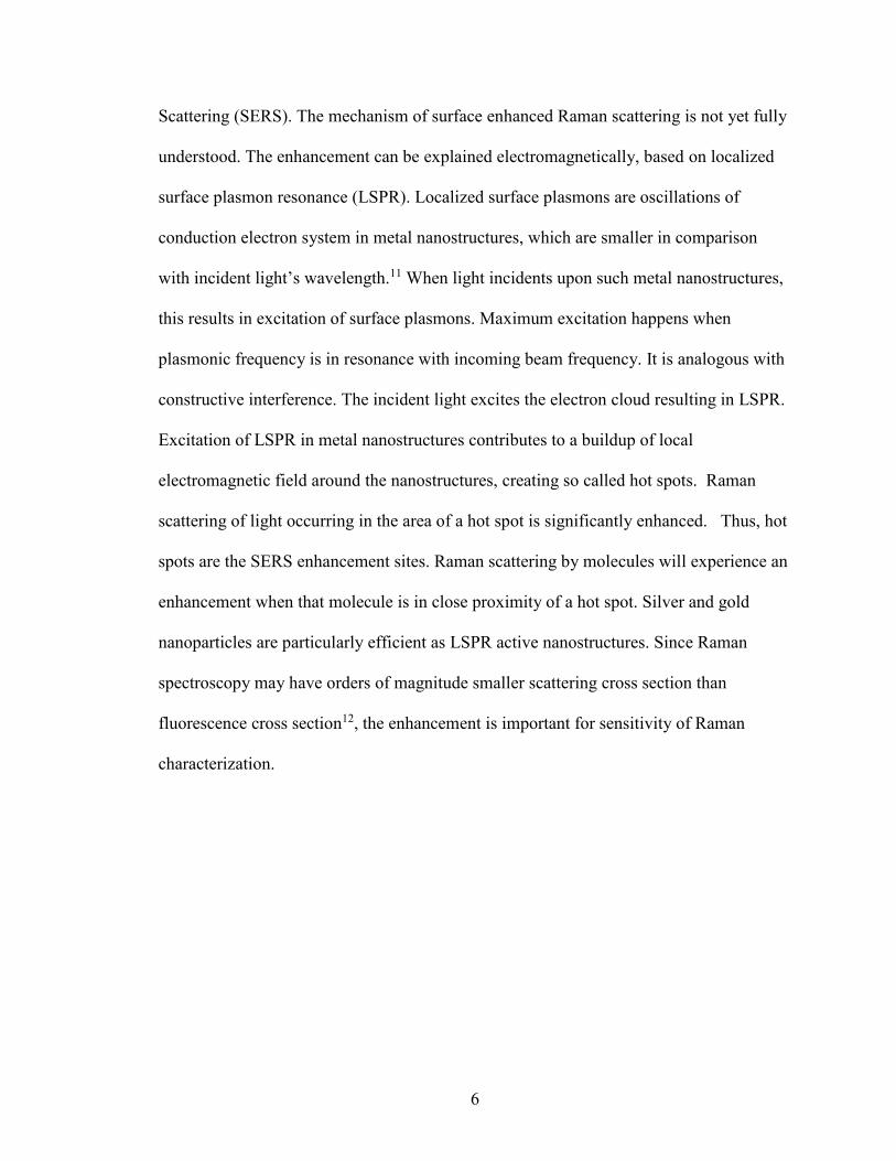
Scattering (SERS). The mechanism of surface enhanced Raman scattering is not yet fully

understood. The enhancement can be explained electromagnetically, based on localized

surface plasmon resonance (LSPR). Localized surface plasmons are oscillations of

conduction electron system in metal nanostructures, which are smaller in comparison

with incident light’s wavelength.11 When light incidents upon such metal nanostructures,

this results in excitation of surface plasmons. Maximum excitation happens when

plasmonic frequency is in resonance with incoming beam frequency. It is analogous with

constructive interference. The incident light excites the electron cloud resulting in LSPR.

Excitation of LSPR in metal nanostructures contributes to a buildup of local

electromagnetic field around the nanostructures, creating so called hot spots. Raman

scattering of light occurring in the area of a hot spot is significantly enhanced. Thus, hot

spots are the SERS enhancement sites. Raman scattering by molecules will experience an

enhancement when that molecule is in close proximity of a hot spot. Silver and gold

nanoparticles are particularly efficient as LSPR active nanostructures. Since Raman

spectroscopy may have orders of magnitude smaller scattering cross section than

fluorescence cross section12, the enhancement is important for sensitivity of Raman

characterization.

7

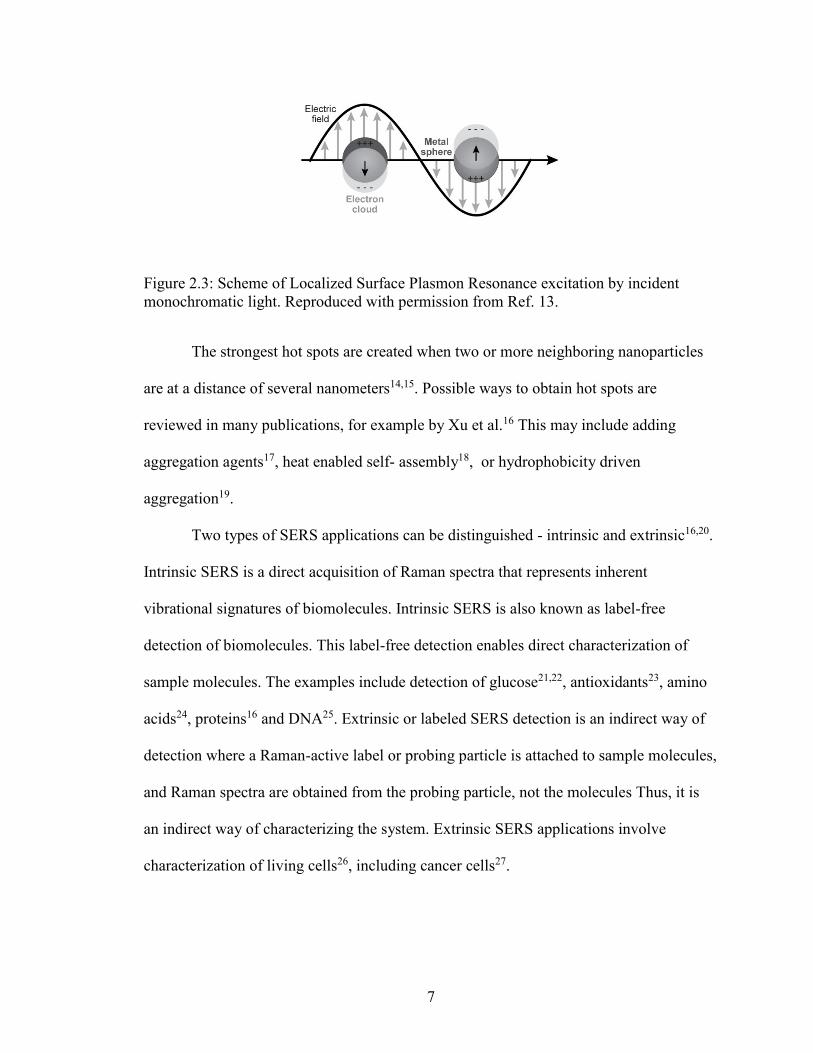
Figure 2.3: Scheme of Localized Surface Plasmon Resonance excitation by incident

monochromatic light. Reproduced with permission from Ref. 13.

The strongest hot spots are created when two or more neighboring nanoparticles

are at a distance of several nanometers14,15. Possible ways to obtain hot spots are

reviewed in many publications, for example by Xu et al.16 This may include adding

aggregation agents17, heat enabled self- assembly18, or hydrophobicity driven

aggregation19.

Two types of SERS applications can be distinguished - intrinsic and extrinsic16,20.

Intrinsic SERS is a direct acquisition of Raman spectra that represents inherent

vibrational signatures of biomolecules. Intrinsic SERS is also known as label-free

detection of biomolecules. This label-free detection enables direct characterization of

sample molecules. The examples include detection of glucose21,22, antioxidants23, amino

acids24, proteins16 and DNA25. Extrinsic or labeled SERS detection is an indirect way of

detection where a Raman-active label or probing particle is attached to sample molecules,

and Raman spectra are obtained from the probing particle, not the molecules Thus, it is

an indirect way of characterizing the system. Extrinsic SERS applications involve

characterization of living cells26, including cancer cells27.

8

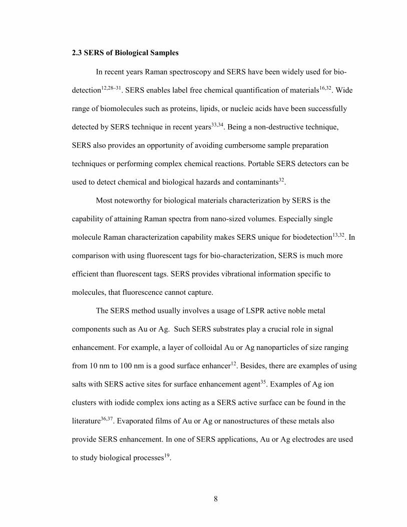
2.3 SERS of Biological Samples

In recent years Raman spectroscopy and SERS have been widely used for bio-

detection12,28–31. SERS enables label free chemical quantification of materials16,32. Wide

range of biomolecules such as proteins, lipids, or nucleic acids have been successfully

detected by SERS technique in recent years33,34. Being a non-destructive technique,

SERS also provides an opportunity of avoiding cumbersome sample preparation

techniques or performing complex chemical reactions. Portable SERS detectors can be

used to detect chemical and biological hazards and contaminants32.

Most noteworthy for biological materials characterization by SERS is the

capability of attaining Raman spectra from nano-sized volumes. Especially single

molecule Raman characterization capability makes SERS unique for biodetection13,32. In

comparison with using fluorescent tags for bio-characterization, SERS is much more

efficient than fluorescent tags. SERS provides vibrational information specific to

molecules, that fluorescence cannot capture.

The SERS method usually involves a usage of LSPR active noble metal

components such as Au or Ag. Such SERS substrates play a crucial role in signal

enhancement. For example, a layer of colloidal Au or Ag nanoparticles of size ranging

from 10 nm to 100 nm is a good surface enhancer12. Besides, there are examples of using

salts with SERS active sites for surface enhancement agent35. Examples of Ag ion

clusters with iodide complex ions acting as a SERS active surface can be found in the

literature36,37. Evaporated films of Au or Ag or nanostructures of these metals also

provide SERS enhancement. In one of SERS applications, Au or Ag electrodes are used

to study biological processes19.

9

In most cases, evaporated films and colloidal nanostructures of Au and Ag have a

larger enhancement than bulk electrodes. The significance of SERS active electrodes is

the possibility to vary the surface potential, which can be used to study charge transfer

mechanism between target molecules and metal surface.

SERS substrates for biological materials should meet certain requirements of size

and shape, and also be compatible with the biomolecules. As a noble metal, gold is inert

against most chemical species, which is a valuable property for SERS biodetection.

Generally, silver is a stronger enhancer than Au, however it oxidizes quickly, for which

reason gold nanoparticles are more suitable for SERS biodetection38.

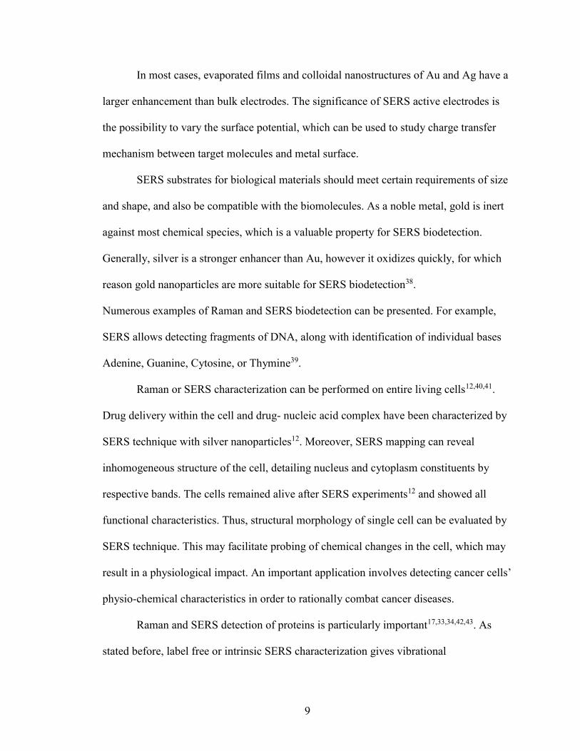
Numerous examples of Raman and SERS biodetection can be presented. For example,

SERS allows detecting fragments of DNA, along with identification of individual bases

Adenine, Guanine, Cytosine, or Thymine39.

Raman or SERS characterization can be performed on entire living cells12,40,41.

Drug delivery within the cell and drug- nucleic acid complex have been characterized by

SERS technique with silver nanoparticles12. Moreover, SERS mapping can reveal

inhomogeneous structure of the cell, detailing nucleus and cytoplasm constituents by

respective bands. The cells remained alive after SERS experiments12 and showed all

functional characteristics. Thus, structural morphology of single cell can be evaluated by

SERS technique. This may facilitate probing of chemical changes in the cell, which may

result in a physiological impact. An important application involves detecting cancer cells’

physio-chemical characteristics in order to rationally combat cancer diseases.

Raman and SERS detection of proteins is particularly important17,33,34,42,43. As

stated before, label free or intrinsic SERS characterization gives vibrational

10

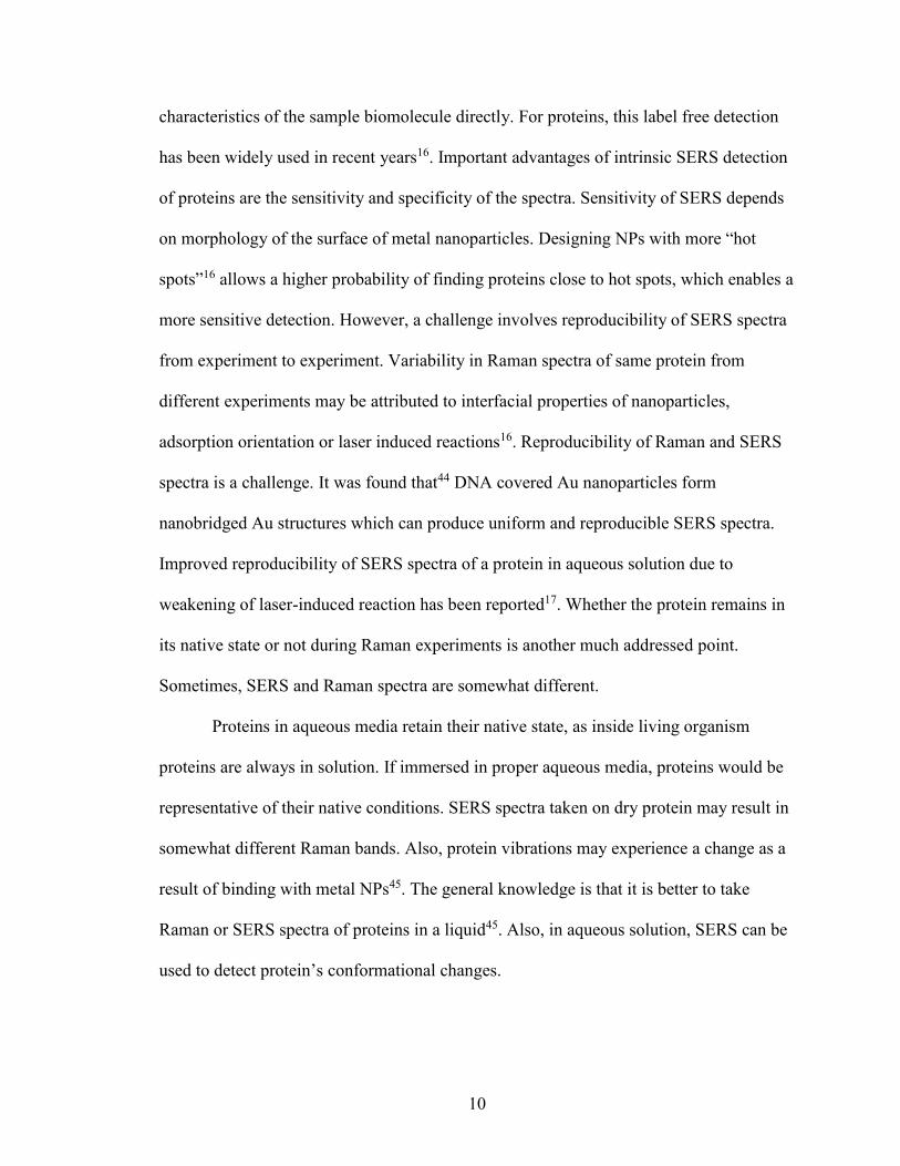
characteristics of the sample biomolecule directly. For proteins, this label free detection

has been widely used in recent years16. Important advantages of intrinsic SERS detection

of proteins are the sensitivity and specificity of the spectra. Sensitivity of SERS depends

on morphology of the surface of metal nanoparticles. Designing NPs with more “hot

spots”16 allows a higher probability of finding proteins close to hot spots, which enables a

more sensitive detection. However, a challenge involves reproducibility of SERS spectra

from experiment to experiment. Variability in Raman spectra of same protein from

different experiments may be attributed to interfacial properties of nanoparticles,

adsorption orientation or laser induced reactions16. Reproducibility of Raman and SERS

spectra is a challenge. It was found that44 DNA covered Au nanoparticles form

nanobridged Au structures which can produce uniform and reproducible SERS spectra.

Improved reproducibility of SERS spectra of a protein in aqueous solution due to

weakening of laser-induced reaction has been reported17. Whether the protein remains in

its native state or not during Raman experiments is another much addressed point.

Sometimes, SERS and Raman spectra are somewhat different.

Proteins in aqueous media retain their native state, as inside living organism

proteins are always in solution. If immersed in proper aqueous media, proteins would be

representative of their native conditions. SERS spectra taken on dry protein may result in

somewhat different Raman bands. Also, protein vibrations may experience a change as a

result of binding with metal NPs45. The general knowledge is that it is better to take

Raman or SERS spectra of proteins in a liquid45. Also, in aqueous solution, SERS can be

used to detect protein’s conformational changes.

11

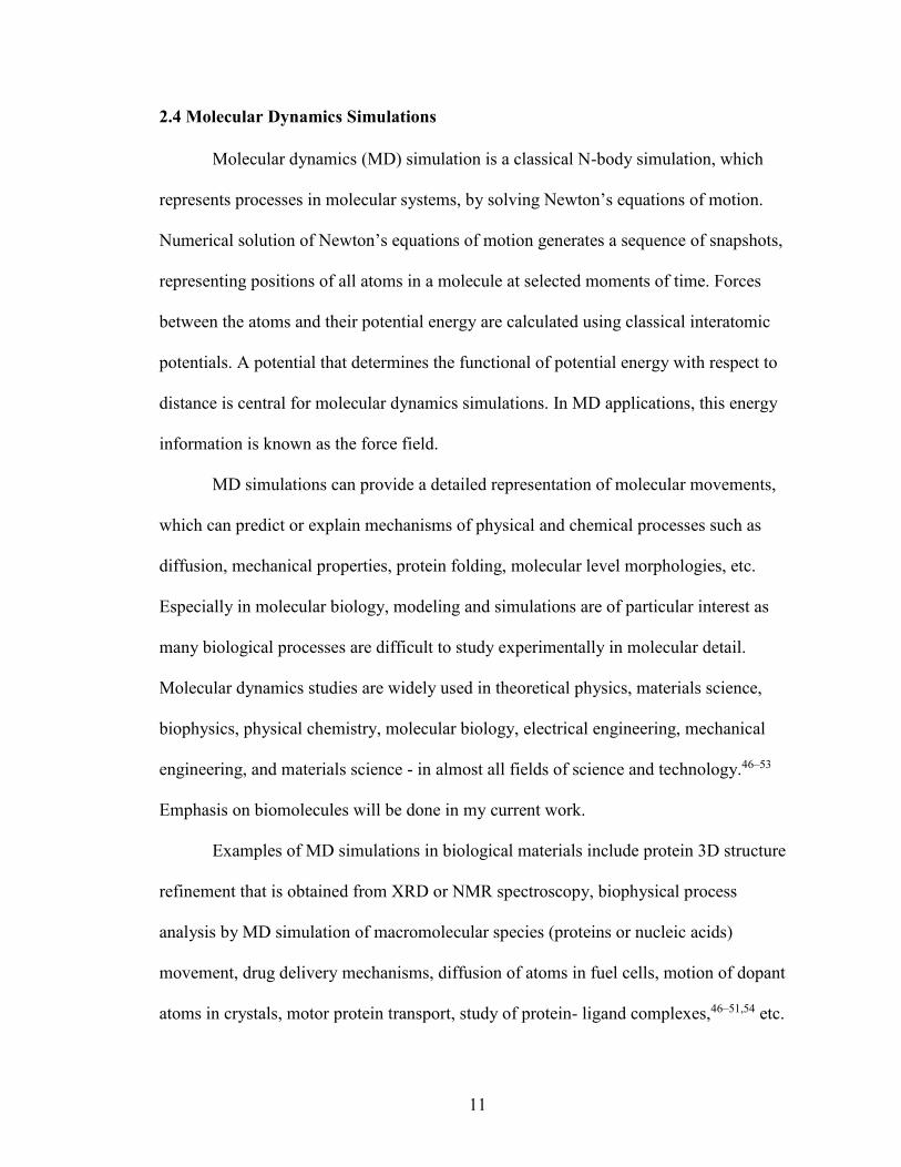
2.4 Molecular Dynamics Simulations

Molecular dynamics (MD) simulation is a classical N-body simulation, which

represents processes in molecular systems, by solving Newton’s equations of motion.

Numerical solution of Newton’s equations of motion generates a sequence of snapshots,

representing positions of all atoms in a molecule at selected moments of time. Forces

between the atoms and their potential energy are calculated using classical interatomic

potentials. A potential that determines the functional of potential energy with respect to

distance is central for molecular dynamics simulations. In MD applications, this energy

information is known as the force field.

MD simulations can provide a detailed representation of molecular movements,

which can predict or explain mechanisms of physical and chemical processes such as

diffusion, mechanical properties, protein folding, molecular level morphologies, etc.

Especially in molecular biology, modeling and simulations are of particular interest as

many biological processes are difficult to study experimentally in molecular detail.

Molecular dynamics studies are widely used in theoretical physics, materials science,

biophysics, physical chemistry, molecular biology, electrical engineering, mechanical

engineering, and materials science - in almost all fields of science and technology.46–53

Emphasis on biomolecules will be done in my current work.

Examples of MD simulations in biological materials include protein 3D structure

refinement that is obtained from XRD or NMR spectroscopy, biophysical process

analysis by MD simulation of macromolecular species (proteins or nucleic acids)

movement, drug delivery mechanisms, diffusion of atoms in fuel cells, motion of dopant

atoms in crystals, motor protein transport, study of protein- ligand complexes,46–51,54 etc.

12

As MD simulations can express positions of atoms as a function of time, it is very useful

to interpret properties of molecular systems. Biophysical phenomena are the best

examples.

Clearly, computational models used in MD may have limitations. Experimental

techniques can be employed to check the validity of numerical predictions. Comparison

between experimental and simulation results either confirms the findings, or serves to

improvement of simulation protocols50,55.

As the potential, or force field, is a key aspect of MD simulations, defining an

approximation of forces between interacting atoms is one of the first steps in MD

protocols. The potentials are editable, i.e. user can change various parameters of the

potential, or force field, according to the needs of the system under consideration.

Outcome of the simulations are accessible by visual software and images of molecular

structure; video of simulation process and data analysis of parameters are the medium of

interpretation of a computational study56.

Karplus et al. suggested three types of applications57 of molecular dynamics in

mesoscopic systems. The first one is determining or refining of structure of a system with

experimentally known parameters using MD. Second usage is describing the system at

equilibrium. The properties that simulation describes are primarily structural and

statistical-mechanical properties. The third application is interpreting the actual dynamics

of a system where particle motion with time is described. First two types can conceivably

be done by kinetic Monte Carlo simulations, whereas the third application is only

possible with an MD simulation.

13

Molecular dynamics simulations for biological materials are made possible by

very powerful and fast computers now-a-days, which enable working with thousands of

atoms, whereas in early days such simulations were limited to a few hundred or even less

atoms. Multiple simulations can be done in parallel to achieve a reliable statistics. There

are many software packages available to simulate not only biological systems, but also

many other complex systems; such as CHARMM, AMBER, GROMACS, NAMD,

YASARA etc.

To understand protein behavior, molecular dynamics is a very efficient tool. As a

protein is a dynamic system that experiences changes of conformations with time,

vibrations of proteins are an interesting subject to investigate. Classical MD can predict

and interpret protein’s dynamic motion. Such detailed molecular-level analysis is difficult

to do experimentally58. Furthermore, the interaction of protein with solvent and ions is

also possible to represent by molecular dynamics simulations. MD simulation can

interpret the solvent dynamics by analyzing motion of individual molecules or ions. The

mechanisms of protein dynamics puzzled scientists for decades. By combining

experimental and simulation techniques, it is now possible to understand dynamical

properties of proteins in details.

2.5. Ferritin and Other Cage Proteins

Ferritin is an intracellular globular cage protein that is found in almost all living

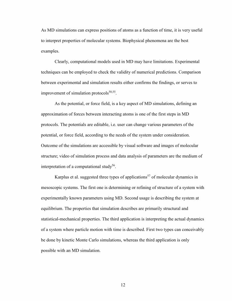
cells. Ferritin consists of 24 sub-units or monomers59–61. Each monomer has four large α-

helices and a also a shorter helix, as shown in Figure 2.4. The monomers self-assemble in

a 4-3-2 symmetric fashion62. In living cells, ferritin works as an iron storage protein59–61

14

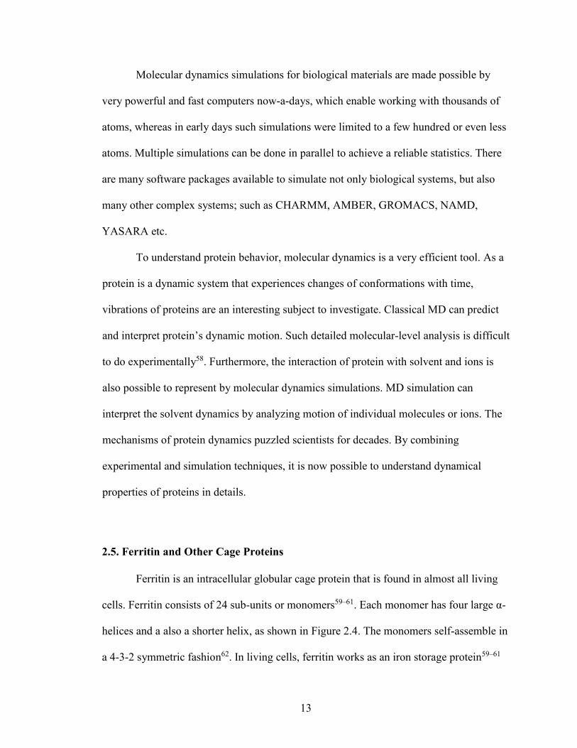
being able to uptake, mineralize and release iron in a controllable manner. Ferritin stores

iron in a form of mineral known as ferrihydrite inside its hollow space. When there is a

deficiency of iron in the cell, ferritin releases iron, and when there is abundance of iron,

ferritin stores extra iron in it. Figure 2.5 shows stored iron mineral cluster inside of a

globule.

The atomic mass of horse ferritin is 440 kDa. It can store up to 4500 iron ions

inside it in the mineralized form. The inside diameter of ferritin’s shell is 8 nm and

outside diameter is 12 nm. The shell is approximately 2 nm thick.

Figure 2.4: Ferritin monomer, PDB ID 5CZU.63 The image was generated using

PYMOL64.

As ferritin consists of 24 monomers, there are three possible structural features on

ferritin surface. They are known as two-fold symmetric junction, three-fold symmetric

junction, and four-fold symmetric junction65. The three and four fold channels form

funnel-like passageways59 that connect interior space with exterior surroundings of the

15

protein, as shown in Figure 2.6. The three-fold channels are hydrophilic in nature, thus

having the ability of passing ions and water molecules, whereas four-fold channels are

hydrophobic, and therefore less efficient in passing charge-bearing species59–61.

The technological significance of ferritin is that it is regarded as an important

constituent for rational design of biomimetic conjugated nano-bio systems. As iron ions

Figure 2.5: Ferrihydrite mineral inside ferritin cage and SEM image of iron loaded

ferritin. Reproduced with permission from Ref. 66.

inside ferritin are stored as ferrihydrite minerals, fully loaded ferritin can work as a

superparamagnetic nanoparticle62. Furthermore, as the ferritin cage has a definite size and

shape, the cavity can incorporate inorganic particles of specific size, making possible

synthesizing nanodot arrays inside the cage65 as Figure 2.7 shows. This way, ferritin can

be used as a template for nanostructure synthesis. The size and shape of nanoparticles

influence electrical, magnetic, optical and other properties. Fabrication process involving

16

Figure 2.6: Ferritin’s 3-fold channel (left) and 4-fold structure (right), PDB ID 5CZU.

The image was generated using JMol67.

ferritin can ensure a uniformity of structure-dependent properties. Many nanoparticles

such as Au, Ag, Pt, Co, Cr, and Zn have already been successfully synthesized utilizing

ferritin-like cavities59,68–70. Crystallized ferritin-like proteins can also act as a membrane,

as the channels can pass ions, atoms, or small nanoparticles65. Ferritin is the most

abundant member of the ferritin superfamily. However, there are many other ferritin-like

cage proteins. The interior hollow space of cage proteins may carry various inorganic

particles, thus making cage proteins a suitable template for nanoparticle synthesis71–74.

Perhaps one of the most promising utilizations of cage proteins is in drug

delivery75. Several advantages enable efficient drug delivery using protein cages.

Nanoparticles are used for drug delivery because of their unique properties related to

small size and surface morphology31,75–77. A narrow size distribution of NPs allows

uniform drug dosing75. However, conventional NPs have some limitations, such as

occasionally wide size distribution, low rate of drug transfer and sometimes instable

17

structure. Caged proteins encapsulating nanoparticles overcome some of these

difficulties31,75,78–80.

Caged proteins are formed by self-assembly of monomers into hollow spherical

globules with uniform interior size. A protein cage may form by monomers of a single

protein, such as ferritin; or by monomers of multiple proteins, for example cowpea

mosaic virus (CPMV)81. Since protein cages have evolved in vivo, their utilization would

involve primarily a selection of functional drug materials to be bonded in three distinct

regions: interior surface, exterior surface, or inter-monomeric interfaces75,79. Control over

functioning of cage proteins facilitates attaining a more efficient drug encapsulation.

Also, by knowing detailed molecular structure and function of the cage channels, it is

possible to control the amount of drug released, and its position in cage proteins82.

2.6. Goals And Objectives Of The Work

The main goal of the work is to improve understanding of structure, dynamics,

and function of ferritin at the molecular level. Specific objectives include the following:

• Performing all-atom molecular dynamic simulations of the interaction of iron ions

with a model of three-fold channel of ferritin responsible for ions’ transport;

• Analysis of molecular details relevant to transport of the ions through the channel

in ferritin;

• Characterization of vibrational properties of iron-loaded ferritin and apo-ferritin

using Raman spectroscopy;

• Comparative analysis of Raman bands of the different ferritin samples, and

interpretation of the results in light of findings of the computational studies;

• Proof-of-principle SERS characterization of ferritin using colloidal gold

nanoparticles for enhancement of Raman signal.

18

Figure 2. 7: Nanodot synthesis using ferritin as a template. Reproduced with permission

from Ref. 65 .

19

CHAPTER 3: EXPERIMENTAL METHODS

3.1. LabRAM HR 800 Evolution Raman Spectroscope

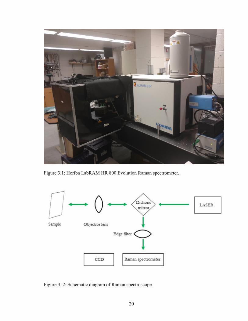
In my work, the Raman characterization was done with Horiba LabRAM HR 800

Evolution Raman spectroscope. A 532 nm green laser was used for the excitation, and the

Stokes scattering was received with edge filter. Among the various types of scattering,

the LabRAM HR Evolution instrument can detect both Stokes and anti-Stokes Raman

scattering, and also fluorescence background. Elastic Rayleigh scattering is blocked by an

Edge filter. Stokes Raman scattering has higher wavelength than the incident beam, and

anti-Stokes scattering has lower wavelength. Band-pass filter of Raman spectroscope

passes only certain wavelengths and absorbs other wavelengths. Edge filter can pass the

Stokes Raman scattering, and notch filter can pass both Stokes and anti-Stokes Raman

scattering. Since in my experiment I used edge filter, only Stokes scattering was detected.

The characterization parameters were optimized for Raman characterization of

liquid samples. Using a 10X microscopic lens facilitated proper focusing of the sample.

A 10 seconds exposure time enabled the laser excitation of the samples. Upon rejection

of elastically scattered light by the edge filter, the light passed through a 300 µm diameter

confocal pinhole upon entering the spectrometer. The Horiba LabRAM 800 Evolution

Raman spectroscope used in my work is shown in Figure 3.1, and a schematic diagram of

Raman spectroscopic technique is shown in Figure 3.2.

20

Figure 3.1: Horiba LabRAM HR 800 Evolution Raman spectrometer.

Figure 3. 2: Schematic diagram of Raman spectroscope.

21

3.2. Sample Preparation

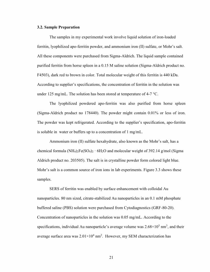
The samples in my experimental work involve liquid solution of iron-loaded

ferritin, lyophilized apo-ferritin powder, and ammonium iron (II) sulfate, or Mohr’s salt.

All these components were purchased from Sigma-Aldrich. The liquid sample contained

purified ferritin from horse spleen in a 0.15 M saline solution (Sigma-Aldrich product no.

F4503), dark red to brown in color. Total molecular weight of this ferritin is 440 kDa.

According to supplier’s specifications, the concentration of ferritin in the solution was

under 125 mg/mL. The solution has been stored at temperature of 4-7 °C.

The lyophilized powdered apo-ferritin was also purified from horse spleen

(Sigma-Aldrich product no 178440). The powder might contain 0.01% or less of iron.

The powder was kept refrigerated. According to the supplier’s specification, apo-ferritin

is soluble in water or buffers up to a concentration of 1 mg/mL.

Ammonium iron (II) sulfate hexahydrate, also known as the Mohr’s salt, has a

chemical formula (NH4)2Fe(SO4)2 · 6H2O and molecular weight of 392.14 g/mol (Sigma

Aldrich product no. 203505). The salt is in crystalline powder form colored light blue.

Mohr’s salt is a common source of iron ions in lab experiments. Figure 3.3 shows these

samples.

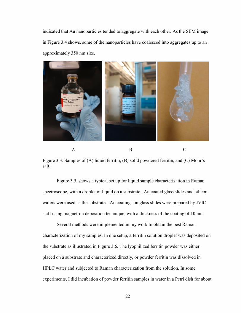
SERS of ferritin was enabled by surface enhancement with colloidal Au

nanoparticles. 80 nm sized, citrate-stabilized Au nanoparticles in an 0.1 mM phosphate

buffered saline (PBS) solution were purchased from Cytodiagnostics (GRF-80-20).

Concentration of nanoparticles in the solution was 0.05 mg/mL. According to the

specifications, individual Au nanoparticle’s average volume was 2.68×105 nm3, and their

average surface area was 2.01×104 nm2. However, my SEM characterization has

22

indicated that Au nanoparticles tended to aggregate with each other. As the SEM image

in Figure 3.4 shows, some of the nanoparticles have coalesced into aggregates up to an

approximately 350 nm size.

A B C

Figure 3.3: Samples of (A) liquid ferritin, (B) solid powdered ferritin, and (C) Mohr’s

salt.

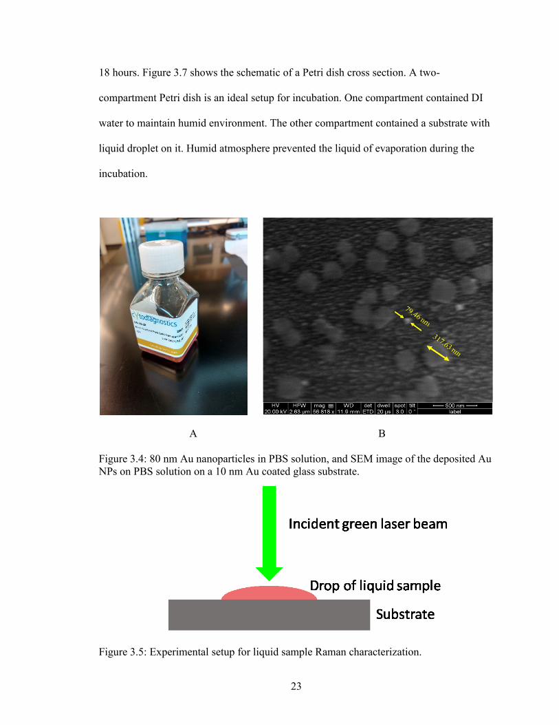
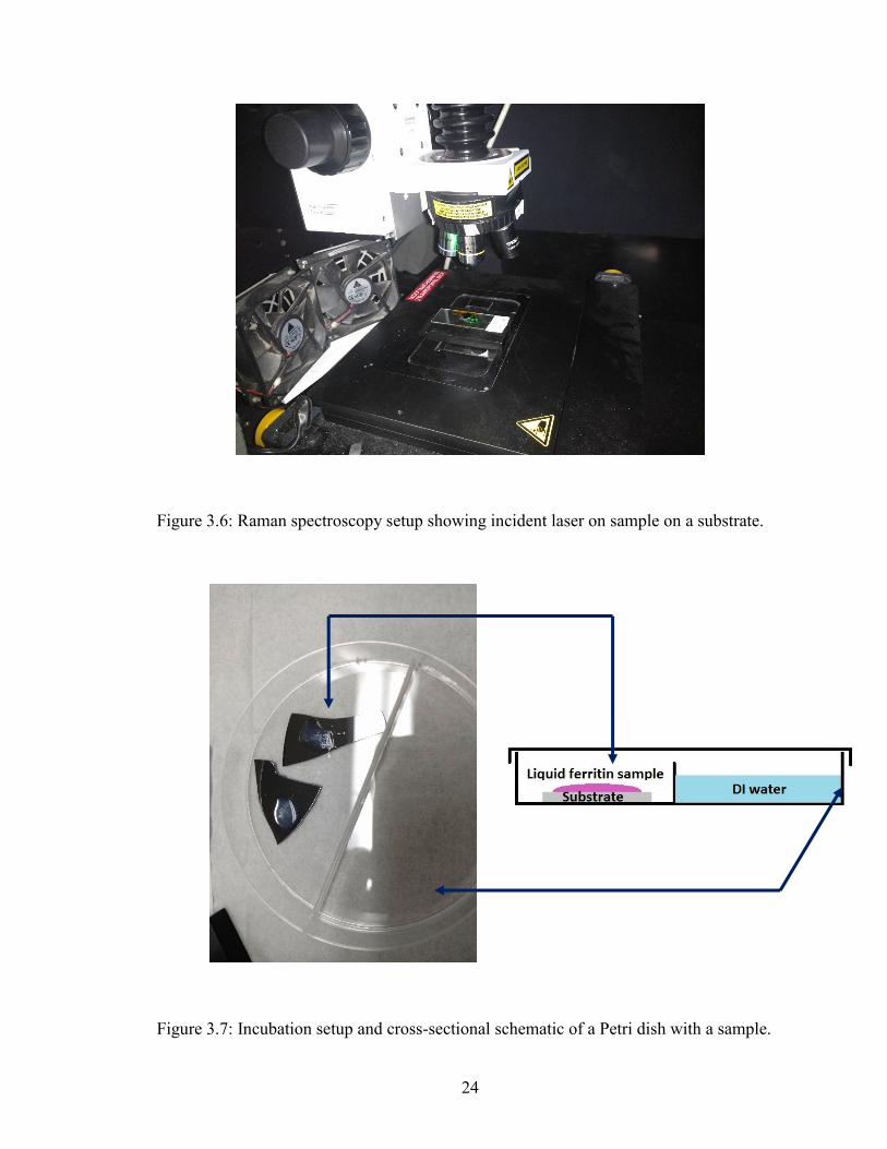
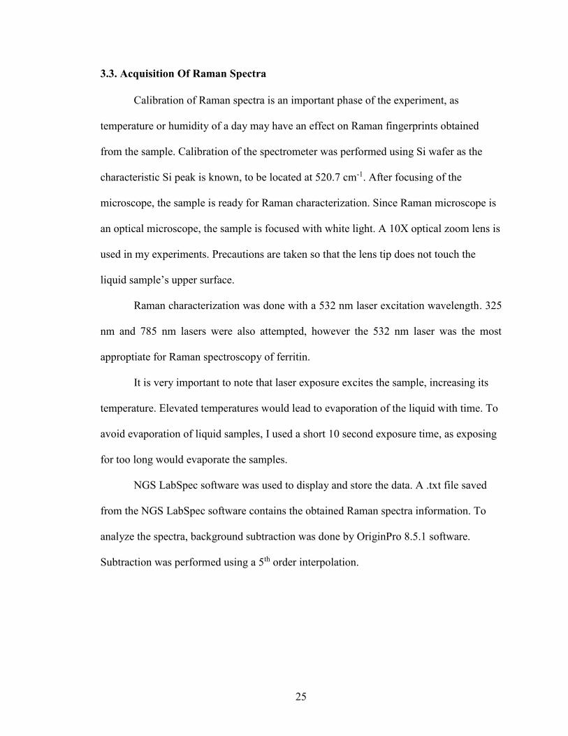
Figure 3.5. shows a typical set up for liquid sample characterization in Raman

spectroscope, with a droplet of liquid on a substrate. Au coated glass slides and silicon

wafers were used as the substrates. Au coatings on glass slides were prepared by JVIC

staff using magnetron deposition technique, with a thickness of the coating of 10 nm.

Several methods were implemented in my work to obtain the best Raman

characterization of my samples. In one setup, a ferritin solution droplet was deposited on

the substrate as illustrated in Figure 3.6. The lyophilized ferritin powder was either

placed on a substrate and characterized directly, or powder ferritin was dissolved in

HPLC water and subjected to Raman characterization from the solution. In some

experiments, I did incubation of powder ferritin samples in water in a Petri dish for about

23

18 hours. Figure 3.7 shows the schematic of a Petri dish cross section. A two-

compartment Petri dish is an ideal setup for incubation. One compartment contained DI

water to maintain humid environment. The other compartment contained a substrate with

liquid droplet on it. Humid atmosphere prevented the liquid of evaporation during the

incubation.

A B

Figure 3.4: 80 nm Au nanoparticles in PBS solution, and SEM image of the deposited Au

NPs on PBS solution on a 10 nm Au coated glass substrate.

Figure 3.5: Experimental setup for liquid sample Raman characterization.

24

Figure 3.6: Raman spectroscopy setup showing incident laser on sample on a substrate.

Figure 3.7: Incubation setup and cross-sectional schematic of a Petri dish with a sample.

25

3.3. Acquisition Of Raman Spectra

Calibration of Raman spectra is an important phase of the experiment, as

temperature or humidity of a day may have an effect on Raman fingerprints obtained

from the sample. Calibration of the spectrometer was performed using Si wafer as the

characteristic Si peak is known, to be located at 520.7 cm-1. After focusing of the

microscope, the sample is ready for Raman characterization. Since Raman microscope is

an optical microscope, the sample is focused with white light. A 10X optical zoom lens is

used in my experiments. Precautions are taken so that the lens tip does not touch the

liquid sample’s upper surface.

Raman characterization was done with a 532 nm laser excitation wavelength. 325

nm and 785 nm lasers were also attempted, however the 532 nm laser was the most

approptiate for Raman spectroscopy of ferritin.

It is very important to note that laser exposure excites the sample, increasing its

temperature. Elevated temperatures would lead to evaporation of the liquid with time. To

avoid evaporation of liquid samples, I used a short 10 second exposure time, as exposing

for too long would evaporate the samples.

NGS LabSpec software was used to display and store the data. A .txt file saved

from the NGS LabSpec software contains the obtained Raman spectra information. To

analyze the spectra, background subtraction was done by OriginPro 8.5.1 software.

Subtraction was performed using a 5th order interpolation.

26

CHAPTER 4: COMPUTATIONAL METHODS

4.1. The GROMACS Molecular Simulation Package

GROMACS83–89, which is an abbreviation from GROningen MAchine for

Chemical Simulations , is a computational package dedicated to molecular dynamics

simulation of biomolecules such as proteins, lipids, and nucleic acids in aqueous

environments. GROMACS solves Newton’s equations of motions for large systems that

may comprise millions of atoms. GROMACS was first designed in 1991 at the

Department of Biophysical Chemistry, University of Groningen, Netherlands, in

association with Computer Science department of the same university, and has been

developed in Groningen University until 2001. Since 2001 it is developed by the

GROMACS development team based in KTH Royal Institute of Technology, Stockholm

University, and Uppsala University in Sweden.

GROMACS’ fast performance is enabled by neighbor search optimization and

inner loop performance optimization.85 The GROMACS package has no built-in force

field of its own; however it is compatible with many force fields such as GROMOS-

9690,91 , OPLS-AA92,93, CHARMM94 and AMBER.95 The forces and energies between

atoms that GROMACS calculates are of three kinds, bonded interaction, non-bonded

interaction and special interaction85. Bonded interaction is the interaction between 2, 3 or

4 atoms following harmonic, cubic or Morse potential. Nonbonded interactions are binary

inter-atomic interactions, obeying a 6-12 Lennard-Jones potential. Special interactions

impose restraints on position, angle or distance of constituents. Position restraints are

important for liquid systems. Decreasing position restraints of a macromolecule in

27

aqueous solution allows the entire system to gradually gain a stable configuration, so that

during subsequent computations the macromolecule remains stable in solution.

GROMACS utilizes a “command line interface”- a text-based command input

system. The user writes text commands, known as scripts. Also, many files containing

topologies and parameters can be used for input and output. Thus, GROMACS is very

user friendly. Errors are instantly detected in the GROMACS platform, and help is

provided in the help section.96 GROMACS gives estimated time of arrival (ETA)

feedback during the simulation processes, indicating how much time is left to complete

the task and when it will be completed. As an output, it generates a trajectory file

containing positions and velocities of atoms in the course of the simulations.

Conventional simulation conditions involve a rectangular simulation box with periodic

boundary conditions, although GROMACS also supports triclinic boxes with periodic

boundary conditions.

GROMACS is an open-source software package, published and distributed with

source codes and documentations under the GNU General Public License85. GROMACS

is mostly run in Linux operating systems. However, from GROMACS 4.5 version, the

program has been extended to be used in Windows OS platform87.

In my work, I used GROMACS 5.1.1 on a Linux cluster equipped with 24 quad-

core - Intel Xeon E5462 CPUs with 2.80 GHz clock-speed, and total RAM of 384 GB.

Along with this, part of my work was done in STAMPEDE2 supercomputer cluster on

Texas Advanced Computing Center (TACC), using GROMACS 5.1.2. STAMPEDE2 is

also a Linux based cluster with Intel Xeon E5-2680 v4 CPUs with 2.40GHz clock speed,

28

and each node having 68 cores. The memory of each node is 96 GB DDR RAM and 16

GB high speed Multi-Channel DRAM, or MCDRAM.

4.2. Preparation Of Model For Simulation

The goal of my MD simulations is to understand how iron ions enter into the

ferritin globular cage and how the iron ions exit from that cage; a long-sought question

that still puzzles the scientific community.

The initial coordinates of atoms in ferritin were obtained from Protein Data Bank,

PDB ID 5CZU.63 After downloading PDB file 5CZU, the file was analyzed. It contained

some hetero atoms (HETATM) which were removed for setting up my system.

Corresponding CONNECT entries were removed as well. This pdb file has a resolution

of 1.6 Å and no atoms or residues were missing, making it an ideal structure to start the

simulation. PDB ID 5CZU is a modified ferritin molecule.63 Residue alanine (Ala119)

was replaced with cysteine. Newly incorporated Cys119 is located close to the C3

symmetric channel of ferritin, and contains Sulphur, which can bind gold surface.

Although binding of modified ferritin to gold is not explored in this work, this capability

is important for future applications. Another cysteine (Cys126) was replaced with alanine

to exclude a possibility of conjugation with a ligand63. The structure was visually

inspected by using visualization software PyMOL64 and VMD56.

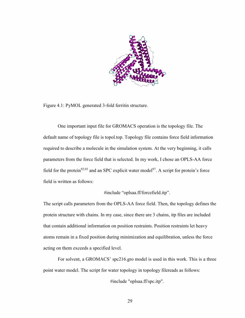
PDB ID 5CZU, as downloaded from the database, contains coordinates of one

subunit. Using PyMOL64, I generated the 3-fold trimeric structure using a symexp

command (Figure 4.1). The command generates neighboring units by utilizing the

symmetry information embedded in the pdb file. This way, from the monomer of ferritin,

one can generate 3-fold trimer, 4-fold tetramer, and even the whole 24-meric globule.

29

Figure 4.1: PyMOL generated 3-fold ferritin structure.

One important input file for GROMACS operation is the topology file. The

default name of topology file is topol.top. Topology file contains force field information

required to describe a molecule in the simulation system. At the very beginning, it calls

parameters from the force field that is selected. In my work, I chose an OPLS-AA force

field for the protein92,93 and an SPC explicit water model97. A script for protein’s force

field is written as follows:

#include “oplsaa.ff/forcefield.itp”.

The script calls parameters from the OPLS-AA force field. Then, the topology defines the

protein structure with chains. In my case, since there are 3 chains, itp files are included

that contain additional information on position restraints. Position restraints let heavy

atoms remain in a fixed position during minimization and equilibration, unless the force

acting on them exceeds a specified level.

For solvent, a GROMACS’ spc216.gro model is used in this work. This is a three

point water model. The script for water topology in topology filereads as follows:

#include "oplsaa.ff/spc.itp".

30

For iron ions, no forcefield is available in GROMACS. I have determined a non-

bonded force field for iron ions based on recently published, extensively optimized

Lennard-Jones parameters98. A GROMACS-format van der Waals radius of 0.24127 nm

and well depth of .039861 kJmol-1 were derived from these data19.

In my simulation work, a 11.24 nm cubic solvation box with periodic boundary

conditions was used. The pdb file with co-ordinates of ferritin’s trimer is transformed into

a GROMACS format “gro” by using a “gmx pdb2gmx” command. The same command

also generates the topology file. The unit cell is constructed using a “gmx editconf”

command. Solvation included addition of water molecules using the “gmx solvate”

command. As the entire system should be charge neutral, I added nine Fe2+ ions, to

neutralize the -18e charge of my system. Ions were added in PyMOL, by using a

“pseudoatom” command.

4.3. Energy Minimization

The purpose of energy minimization is to relax the protein structure. Before

adding any water in the solvation box, in-vacuo energy minimization was performed with

position restraints to avoid distortion of protein structure. The force constant for each

non- hydrogen atom in protein molecule was equal to 100000 kJmol-1nm-2 during in-

vacuo minimization, which is a very strong position restraints required to keep the protein

stable in vacuum. The minimization had a converging limit of 10 kJmol-1nm-1 maximum

force.

After the water molecules and ions were added, energy minimization of the

solvated system was done with six gradually decreasing position restraints on non-

31

hydrogen atoms of ferritin. Position restraints involved a force constant value decrement

of 10 times in each successive step except for the last one, where no restraints were

applied. The force constants were equal to 100000, 10000, 1000, 100, 10 and 0 kJmol-

1nm-2 in the respective six steps of minimization. Starting with a strong position restraint

on protein atoms, the minimization proceeded with gradually weakening position

restraints. Each minimization involved a maximum number of 3000 steepest descent

steps. Minimization may converge before reaching the maximum number of steps, and in

my case, this happened in later steps. The steepest descent step size was 0.01 nm, up to

allowing a maximum force of 10 kJmol-1nm-1.

Energy minimizations were executed by first using “gmx grompp” command with

a minimization parameter .mdp file. The command “gmx grompp” assembles the protein

structure, topology of the system and all simulation parameters into a binary input file

called tpr file. Then the minimizations are done in GROMACS MD engine, executing

with “gmx mdrun” command. The command “gmx mdrun” initiates GROMACS MD

engine to run the molecular dynamics. Using the flag “-v” in the script is an optional flag,

used to show when the simulation will end and show progression of steps as well, the

ETA feedback capability of Gromacs I mentioned earlier. The “&” symbol at the end of

the script is used to run the process in background. So that I can log off from the server

but still the simulation will continue.

After the energy minimization process, a .gro file containing minimized structure

is generated.

32

4.4. Equilibration

After energy minimization is completed, the system is ready for equilibration.

Energy minimization provided an initial relaxation of the protein structure. Now, it is

important to equilibrate water molecules and iron ions added in the system. Equilibration

ensures stability of the system during subsequent production molecular dynamics

simulations. In the course of equilibration, temperature is gradually increased in the

system up to the level of 310K, at which production MD will be done. Pressure will be

also maintained at 1 bar.

I applied the NVT ensemble (number of particles, volume, and temperature

constant) using a thermostat with velocity rescaling99. Initial velocities of atoms in the

system were set at random using a procedure called seed generation. Varying seed

generation results in simulations with similar initial positions, but different initial

velocities of atoms. In my work, three trajectories with different seed generation were

generated for each model. During the first NVT equilibration step, temperature was

raised to 310K. After the initial NVT step, I used six successive NVT equilibration steps

with decreasing position restraints on non-hydrogen atoms of the protein. Similarly, as

for energy minimization. The force constants in each step were similar as for energy

minimization: 100000, 10000, 1000, 100, 10 and 0 kJmol-1nm-2. The temperature

coupling time for each NVT equilibration was equal to 0.01 ps. The number of MD steps

for the first NVT equilibration was 50000, i.e. 100 ps; and each subsequent NVT

equilibration comprised 25000 MD steps, i.e. 50 ps each; making the entire NVT

equilibration process 400 ps long.

33

Next, NPT ensemble (number of particles, pressure, and temperature constant)

was used for equilibration at 1 bar with Parinello-Rahman barostat100,101, also using

velocity rescaling to maintain temperature at 310 K. 50000 integration steps were

performed, totaling 100 ps of NPT equilibration. The temperature and pressure coupling

time in NPT equilibration were equal to 0.1 pseach. The compressibility was equal to

0.000045 bar-1.

To do NVT and NPT equilibration, a “gmx grompp” command was used to

generate a binary edr file. Then “gmx mdrun” command started the GROMACS MD

engine for equilibration. During NPT equilibration, while using a “gmx grompp”

command, an additional “-t” flag was used to load velocities generated during previous

NVT steps, and other parameters. The resulting structure was ready for production MD

simulations.

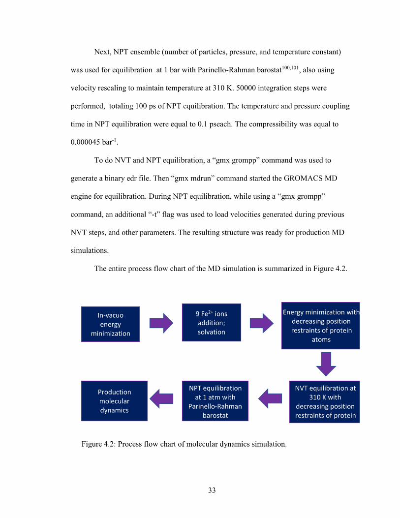
The entire process flow chart of the MD simulation is summarized in Figure 4.2.

Figure 4.2: Process flow chart of molecular dynamics simulation.

In-vacuo energy

minimization

9 Fe2+ ions addition; solvation

Energy minimization with decreasing position restraints of protein

atoms

NVT equilibration at 310 K with

decreasing position restraints of protein

atoms

NPT equilibration at 1 atm with

Parinello-Rahman barostat

Production molecular dynamics

34

4.5. Production MD Simulations

After successful equilibration, molecular dynamics simulations were performed

to generate time series of all atoms’ positions and velocities, known as MD trajectories.

The GROMACS MD engine was used. The protocol was similar to the equilibration

steps, involving “gmx grompp” and “gmx mdrun” commands. The output (checkpoint)

file generated after NPT equilibration was loaded as an input using a “-t” flag.

An integration time-step of 2 fs was used for all MD simulations. For neighbor

searching in MD process, a Verlet cutoff-scheme was employed. An 1.4 nm cutoff radius

was used for van der Waals and short-range electrostatic interactions. Long range

electrostatic interactions were accounted for with a particle-mesh Ewald (PME)

summation using a 4th-order interpolation and a maximum grid dimension of 0.135 nm.

The neighbor list was updated after every 10 integration time-steps, or 20 fs. The LINCS

algorithm102 with 4th order expansion and 2 iterations was used to constrain bond lengths

for the protein. Water molecules were constrained with the SETTLE algorithm103.

In my production MD simulations, a physiologically relevant temperature of 310

K was maintained using a velocity rescaling thermostat with a stochastic term99 ensuring

a proper canonical ensemble. Protein and non-protein groups were coupled separately to

respective temperature baths. Pressure of 1 atm was maintained with a Parrinello-Rahman

barostat100,101. Other details of maintaining temperature and pressure can be found in

Section 4.4.

Production MD was performed long enough to obtain a desired duration of MD

trajectories. Continuation of interrupted simulation is possible by loading output data

from previous production MD runs.

35

Output generated after production MD simulations includes a binary full precision

trajectory file containing time dependent coordinates and velocities of each atom.

Visualization software such as VMD reads this file, displays graphical animation of the

process, and provides analysis of the results.

4.6. Visualization And Analysis Softwares

Data files that are used in GROMACS for input or output are either ASCII or

binary, and they contain coordinates and velocities information. Analyzing this

information reveals the nature of chemical or physical processes represented by the

simulation. Initial step in this analysis is to visually inspect the process under

investigation. Table 4.1 lists visualization software that was extensively used in my work,

and specific functions that I used. A lot of analyses beyond simple visualization can be

done in each software. Note that sometimes, one software is better suited than other to

perform a certain task.

Using VMD 1.9.2, I rendered the trajectory animation as a movie by using VMD

movie maker extension tool. VMD is also extensively used in my work for post

simulation analyses. Using snapshot rendering mode with trajectory loading settings, I

used VMD to take screenshots of each timesteps and then by using VideoMach software,

those screenshots were compiled together to create the movie. Also, by using VMD, I

visually represented the protein in many user controlled ways- varying atom rendering

options in different ways and by applying different colors in each atom-type or residue-

type or any other subset of similar atoms. I utilized VMD’s graphical interface for

performing structural analysis. Also, VMD’s text interface enabled by Tcl embeddable

36

parser were extensively used. This interface allows inputting script commands for

complex functions, such as selecting atoms up to certain distance form a reference point,

removing particular molecules or residues, measuring distance between two atoms,

zooming in the chemical structure with same magnification, etc. It was used to

specifically show secondary structures, side chains, solvent accessible surface area

(SASA), electrostatic potential on the surface, diffusion path of an ion or atom, etc. It

should be noted that, merely visualizing protein in different ways is only a small part of

vast analyses possible to do in VMD. For example, radial pair distribution function and

RMSD trajectory tool were also used in my work to generate RDF and RMSD plots of

water molecules and iron ions respectively. RDF is enabled by an extension tool,

measuring distribution of one atom type with respect to another atom type. I measured

g(r), the radial pair distribution function of oxygen atom of water molecules with respect

to iron ion that enters into the channel. The result of my RDF analysis of water solvation

shell is briefly discussed in chapter 5. This RDF plot is generated over a time frame,

which can be specified in VMD command prompt. I also used RMSD trajectory tool to

generate RMSD plot of iron ions. The tool is capable of skipping time frames, thus

accommodating large trajectories with many MD steps, for example in my case around

24 ns of simulation trajectories. “All to all” RMSD is possible, i.e. all molecules against

all molecules or all frames against all frames. I did RMSD of iron ion that enters the

channel, with respect to its first frame against all frames. Multiplot VMD plugin

composes the coordinate data file, accessible as .txt format for MS Excel. No selection

modifiers were used in my analysis as the analysis is limited to one ion at a time.104,105

37

The STRIDE algorithm106 as implemented in VMD was used to identify protein’s

secondary structures.

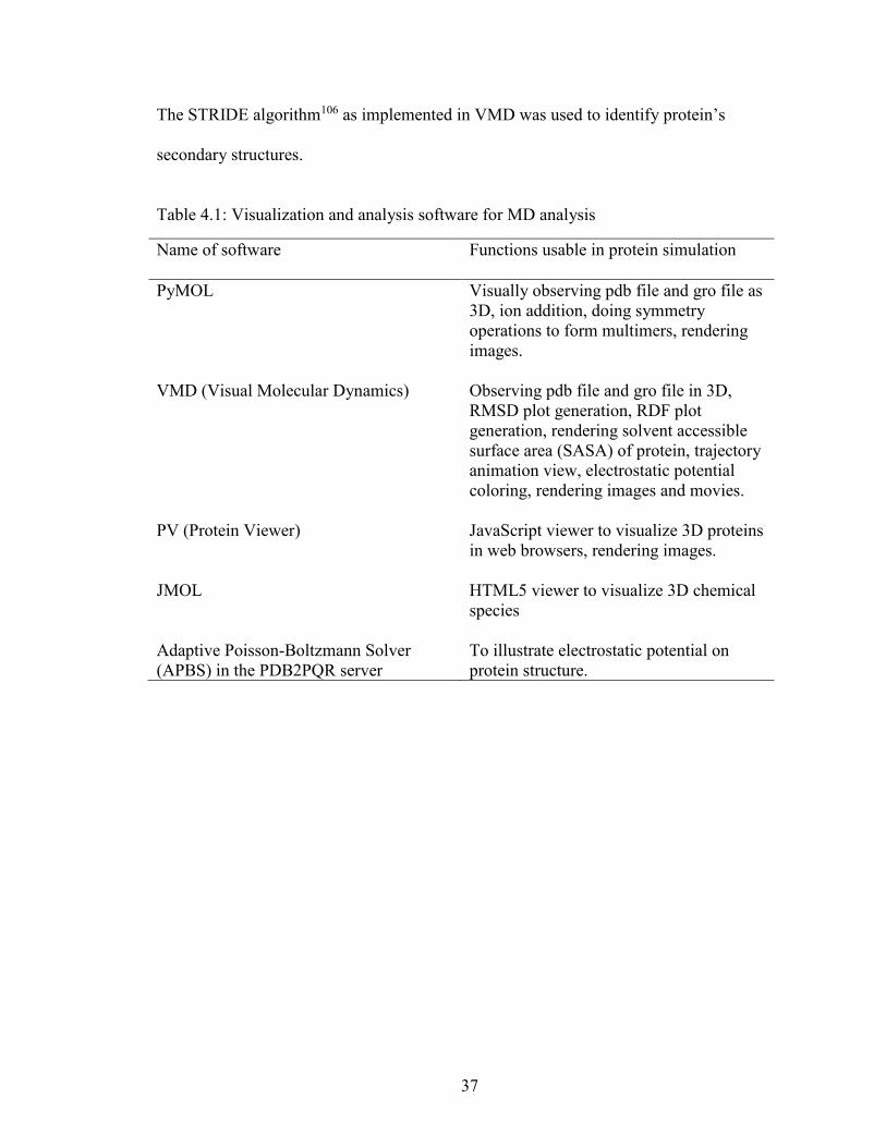
Table 4.1: Visualization and analysis software for MD analysis

Name of software Functions usable in protein simulation

PyMOL Visually observing pdb file and gro file as

3D, ion addition, doing symmetry

operations to form multimers, rendering

images.

VMD (Visual Molecular Dynamics) Observing pdb file and gro file in 3D,

RMSD plot generation, RDF plot

generation, rendering solvent accessible

surface area (SASA) of protein, trajectory

animation view, electrostatic potential

coloring, rendering images and movies.

PV (Protein Viewer) JavaScript viewer to visualize 3D proteins

in web browsers, rendering images.

JMOL HTML5 viewer to visualize 3D chemical

species

Adaptive Poisson-Boltzmann Solver

(APBS) in the PDB2PQR server

To illustrate electrostatic potential on

protein structure.

38

CHAPTER 5: COMPUTATIONAL RESULTS

5.1. Transport Of Fe Ions Through Ferritin’s Channel

The ferritin monomer of PDB ID 5CZU was used to construct the 3-fold structure

expressing the channel responsible for transport of iron ions, as described in Sect. 4.2.

The trimer structure contains only atoms of the protein. Some atoms belong to main chain

of the protein, and others to side chains.

After solvation, 9 Fe2+ ions were added in the solvation box. In one setup, ions

were added outside the hypothetical ferritin globule, i.e. on the convex side of the 3-fold

channel, as shown in Figure 5.1(A, B). The approximate distance of Fe2+ ions from the

channel was 0.5-1.1 nm. In another setup, I added Fe2+ ions on the concave side of the

channel, mimicking ions added inside the hypothetical ferritin globule. In the course of

NPT and NVT equilibrations the ions have moved, still remaining in close vicinity of the

channel (Figure 5.2).

As I applied three different sets of initial velocities of atoms with the same initial

positions, three statistically independent MD trajectories were produced for each

structure. I denote the three trajectories for ions added outside of the trimer by OA, OB,

and OC. Similarly, three trajectories for ions added inside are denoted by IA, IB, and IC.

Table 5.1 lists the six trajectories obtained. At least 20 ns of simulations were completed

for each of the trajectories. I found similar result for all three sets in most cases. Unless

otherwise mentioned, I are displaying results of OA and IA trajectories as a

representative outcome of my simulations.

39

Figure 5.1: Initial structures of ferritin’s trimer with nine iron ions before equilibration:

A) Fe2+ ions added outside of the ferritin trimer, B) side view of ions outside the trimer,

C) Fe2+ ions added inside of the ferritin trimer, D) side view of ions inside the trimer.

Iron ions are shown with red spheres.

Figure 5.3 shows snapshots from production MD trajectory OA. It can be seen

that at 1.4 ns, one of the ions almost entered the channel, and a second ion approached it.

During subsequent simulations, the first ion remained in the channel, and the second one

continued approaching it. The second ion entered the channel after approximately 1.5 ns

from the beginning of production simulations.

40

Figure 5.2: Iron ion positions after equilibration: A) ions added outside of the trimer, B)

ions added outside side view, C) ions added inside of the trimer, D) ions added inside

side view. Ions are shown by red spheres.

As the second ion moves into the channel, it repeals the first ion inside the

channel. At approximately 11.8 ns, the first ion completely exited from the channel,

expelled by the second ion. Simulation up to 20 ns shows a complete expulsion of the

first ion. A similar trend was observed in two other trajectories OB and OC, with ions

41

entering the channel in less than 2 ns. In trajectory OC the first ion did not yet fully exit

by 20 ns, however it was in the process of ejection from the channel. In trajectory OB the

first ion completely exited from the channel by approximately 8.8 ns, expelled by the

second ion; and the third ion entered the channel at 4.2 ns. By 20 ns both the second and

the third ion remained inside the channel, following the path of the first ion.

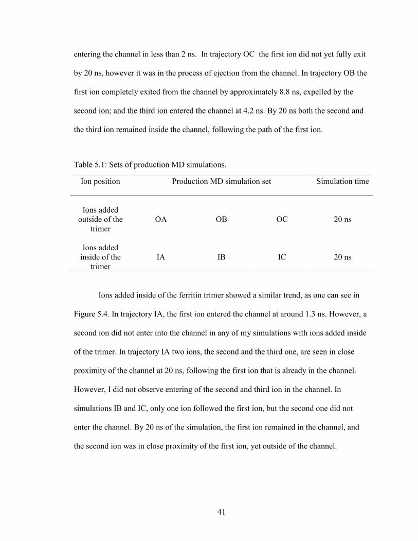
Table 5.1: Sets of production MD simulations.

Ion position Production MD simulation set Simulation time

Ions added

outside of the

trimer

OA

OB

OC

20 ns

Ions added

inside of the

trimer

IA

IB

IC

20 ns

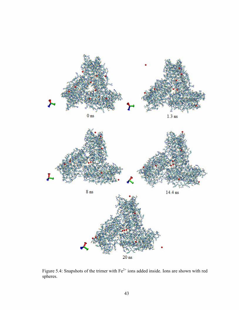
Ions added inside of the ferritin trimer showed a similar trend, as one can see in

Figure 5.4. In trajectory IA, the first ion entered the channel at around 1.3 ns. However, a

second ion did not enter into the channel in any of my simulations with ions added inside

of the trimer. In trajectory IA two ions, the second and the third one, are seen in close

proximity of the channel at 20 ns, following the first ion that is already in the channel.

However, I did not observe entering of the second and third ion in the channel. In

simulations IB and IC, only one ion followed the first ion, but the second one did not

enter the channel. By 20 ns of the simulation, the first ion remained in the channel, and

the second ion was in close proximity of the first ion, yet outside of the channel.

42

Figure 5.3: Snapshots of the trimer with Fe2+ ions added outside at different simulation

times.

43

Figure 5.4: Snapshots of the trimer with Fe2+ ions added inside. Ions are shown with red

spheres.

44

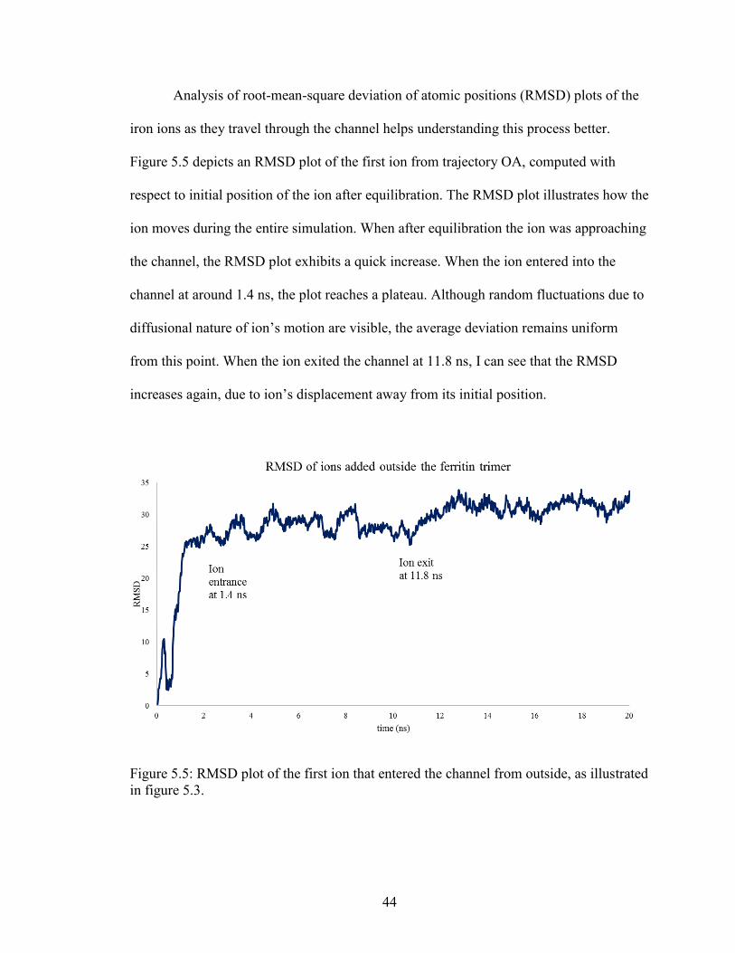
Analysis of root-mean-square deviation of atomic positions (RMSD) plots of the

iron ions as they travel through the channel helps understanding this process better.

Figure 5.5 depicts an RMSD plot of the first ion from trajectory OA, computed with

respect to initial position of the ion after equilibration. The RMSD plot illustrates how the

ion moves during the entire simulation. When after equilibration the ion was approaching

the channel, the RMSD plot exhibits a quick increase. When the ion entered into the

channel at around 1.4 ns, the plot reaches a plateau. Although random fluctuations due to

diffusional nature of ion’s motion are visible, the average deviation remains uniform

from this point. When the ion exited the channel at 11.8 ns, I can see that the RMSD

increases again, due to ion’s displacement away from its initial position.

Figure 5.5: RMSD plot of the first ion that entered the channel from outside, as illustrated

in figure 5.3.

45

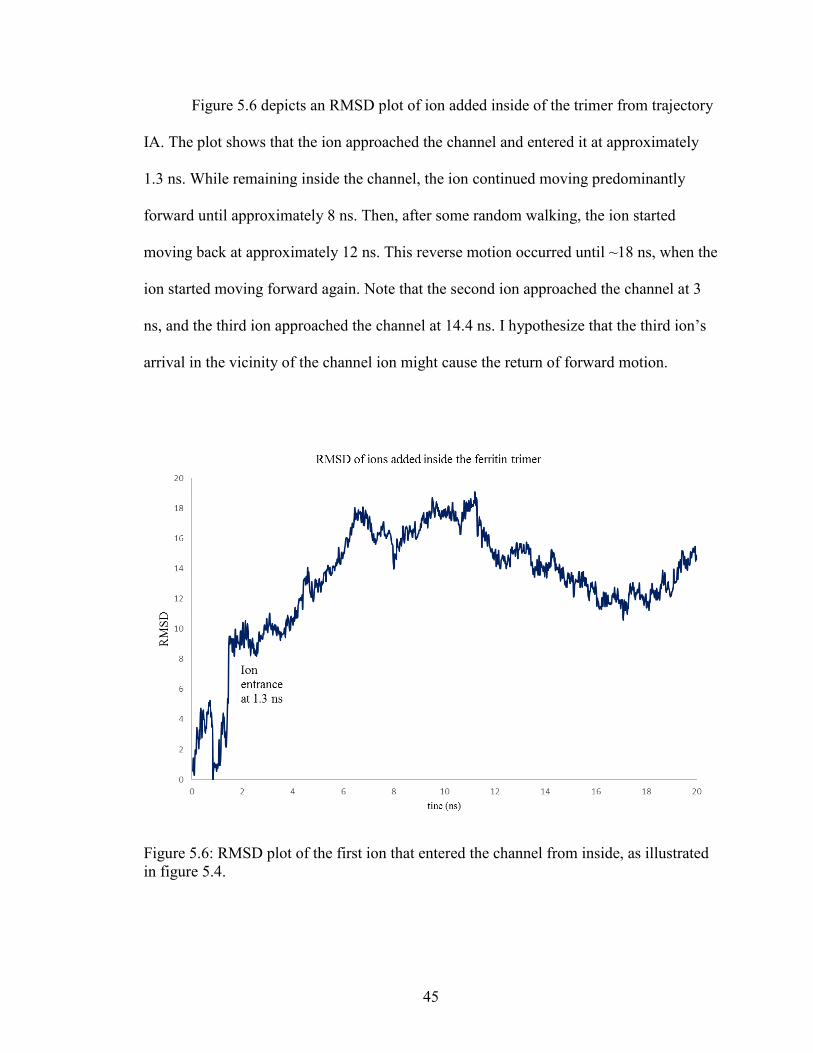
Figure 5.6 depicts an RMSD plot of ion added inside of the trimer from trajectory

IA. The plot shows that the ion approached the channel and entered it at approximately

1.3 ns. While remaining inside the channel, the ion continued moving predominantly

forward until approximately 8 ns. Then, after some random walking, the ion started

moving back at approximately 12 ns. This reverse motion occurred until ~18 ns, when the

ion started moving forward again. Note that the second ion approached the channel at 3

ns, and the third ion approached the channel at 14.4 ns. I hypothesize that the third ion’s

arrival in the vicinity of the channel ion might cause the return of forward motion.

Figure 5.6: RMSD plot of the first ion that entered the channel from inside, as illustrated

in figure 5.4.

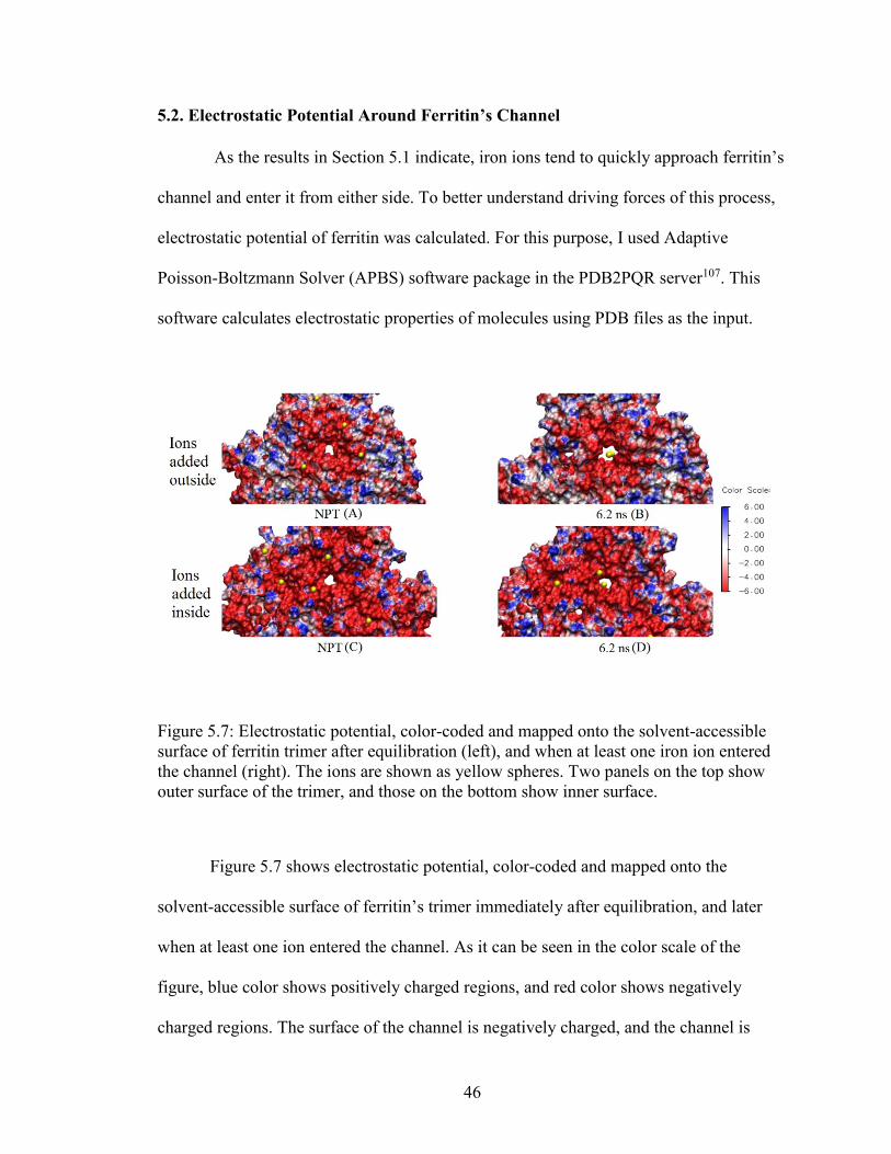
46

5.2. Electrostatic Potential Around Ferritin’s Channel

As the results in Section 5.1 indicate, iron ions tend to quickly approach ferritin’s

channel and enter it from either side. To better understand driving forces of this process,

electrostatic potential of ferritin was calculated. For this purpose, I used Adaptive

Poisson-Boltzmann Solver (APBS) software package in the PDB2PQR server107. This

software calculates electrostatic properties of molecules using PDB files as the input.

Figure 5.7: Electrostatic potential, color-coded and mapped onto the solvent-accessible

surface of ferritin trimer after equilibration (left), and when at least one iron ion entered

the channel (right). The ions are shown as yellow spheres. Two panels on the top show

outer surface of the trimer, and those on the bottom show inner surface.

Figure 5.7 shows electrostatic potential, color-coded and mapped onto the

solvent-accessible surface of ferritin’s trimer immediately after equilibration, and later

when at least one ion entered the channel. As it can be seen in the color scale of the

figure, blue color shows positively charged regions, and red color shows negatively

charged regions. The surface of the channel is negatively charged, and the channel is

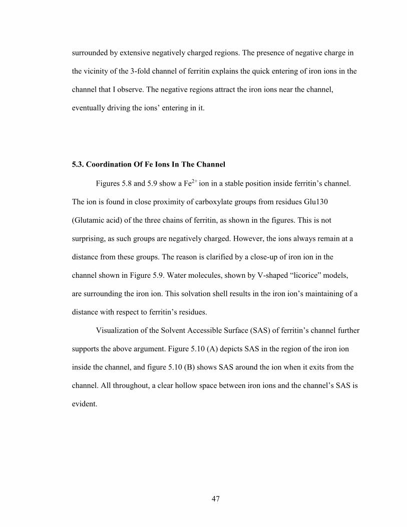
47

surrounded by extensive negatively charged regions. The presence of negative charge in

the vicinity of the 3-fold channel of ferritin explains the quick entering of iron ions in the

channel that I observe. The negative regions attract the iron ions near the channel,

eventually driving the ions’ entering in it.

5.3. Coordination Of Fe Ions In The Channel

Figures 5.8 and 5.9 show a Fe2+ ion in a stable position inside ferritin’s channel.

The ion is found in close proximity of carboxylate groups from residues Glu130

(Glutamic acid) of the three chains of ferritin, as shown in the figures. This is not

surprising, as such groups are negatively charged. However, the ions always remain at a

distance from these groups. The reason is clarified by a close-up of iron ion in the

channel shown in Figure 5.9. Water molecules, shown by V-shaped “licorice” models,

are surrounding the iron ion. This solvation shell results in the iron ion’s maintaining of a

distance with respect to ferritin’s residues.

Visualization of the Solvent Accessible Surface (SAS) of ferritin’s channel further

supports the above argument. Figure 5.10 (A) depicts SAS in the region of the iron ion

inside the channel, and figure 5.10 (B) shows SAS around the ion when it exits from the

channel. All throughout, a clear hollow space between iron ions and the channel’s SAS is

evident.

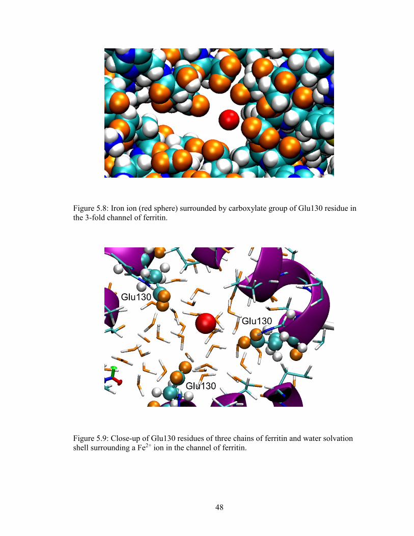
48

Figure 5.8: Iron ion (red sphere) surrounded by carboxylate group of Glu130 residue in

the 3-fold channel of ferritin.

Figure 5.9: Close-up of Glu130 residues of three chains of ferritin and water solvation

shell surrounding a Fe2+ ion in the channel of ferritin.

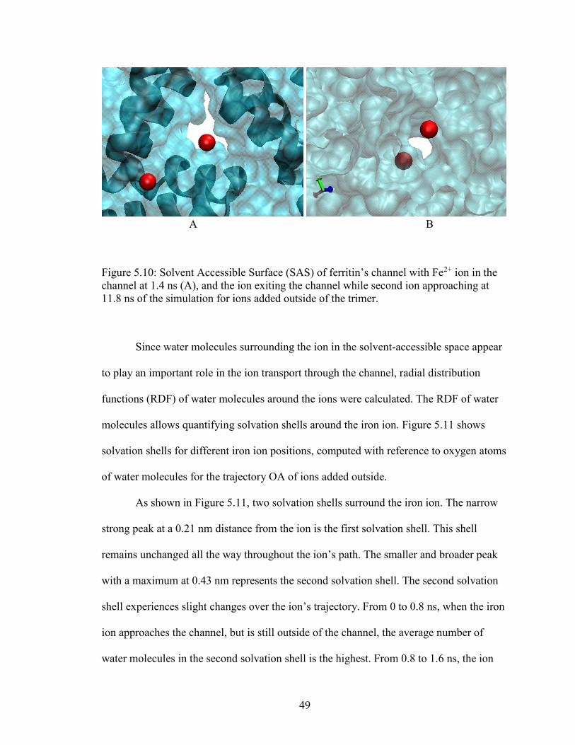
49

A B

Figure 5.10: Solvent Accessible Surface (SAS) of ferritin’s channel with Fe2+ ion in the

channel at 1.4 ns (A), and the ion exiting the channel while second ion approaching at

11.8 ns of the simulation for ions added outside of the trimer.

Since water molecules surrounding the ion in the solvent-accessible space appear

to play an important role in the ion transport through the channel, radial distribution

functions (RDF) of water molecules around the ions were calculated. The RDF of water

molecules allows quantifying solvation shells around the iron ion. Figure 5.11 shows

solvation shells for different iron ion positions, computed with reference to oxygen atoms

of water molecules for the trajectory OA of ions added outside.

As shown in Figure 5.11, two solvation shells surround the iron ion. The narrow

strong peak at a 0.21 nm distance from the ion is the first solvation shell. This shell

remains unchanged all the way throughout the ion’s path. The smaller and broader peak

with a maximum at 0.43 nm represents the second solvation shell. The second solvation

shell experiences slight changes over the ion’s trajectory. From 0 to 0.8 ns, when the iron

ion approaches the channel, but is still outside of the channel, the average number of

water molecules in the second solvation shell is the highest. From 0.8 to 1.6 ns, the ion

50

entered into the channel. Narrow channel pathway results in slightly lesser average

number of water molecules in the second solvation shell. The ion exits the channel

between 11 and 11.8 ns, and the RDF plot shows an increased number of water

molecules. After 20 ns, I can see more water molecules surrounding the ion.

Figure 5.12 presents an RDF plot of trajectory IA (ions added inside of the trimer),

calculated for the iron ion that entered the channel, with reference to oxygen atoms of

water molecules. Two solvation shells are clearly visible. The first solvation shell

remains unchanged throughout the trajectory, and the second one exhibit slight changes.

When the ion enters I channel, I can see more water molecules in second solvation shell.

During subsequent simulations, ion remains inside the narrow channel, resulting in a

somewhat lesser number of water molecules in second solvation shell.

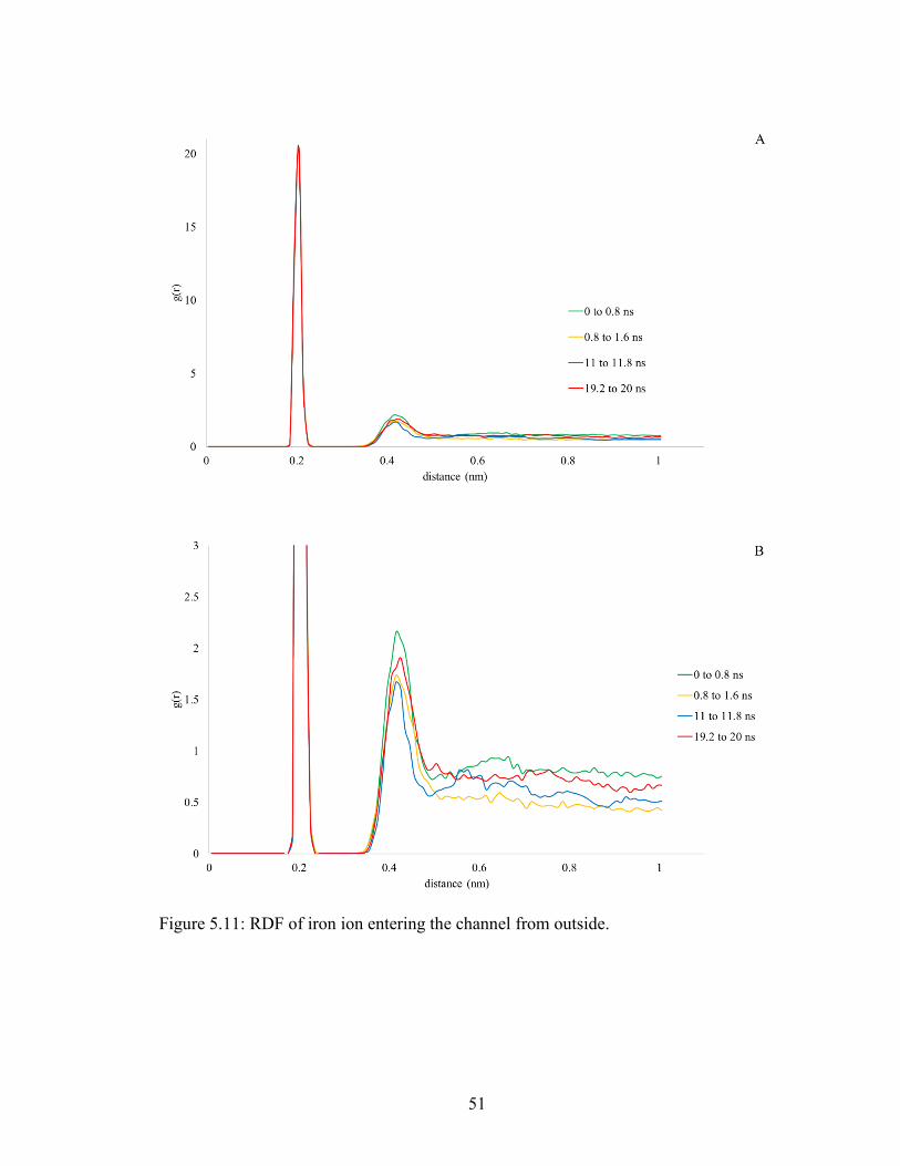
51

Figure 5.11: RDF of iron ion entering the channel from outside.

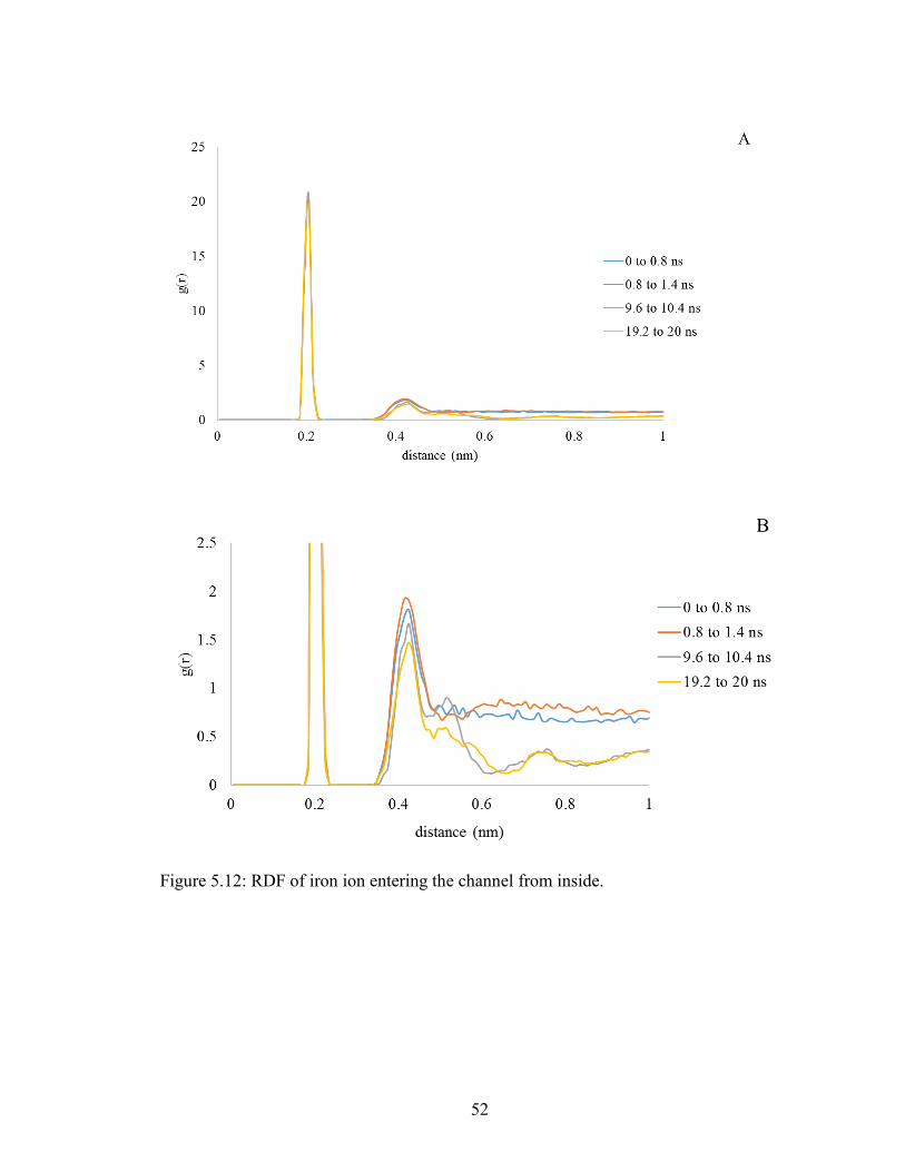
52

Figure 5.12: RDF of iron ion entering the channel from inside.

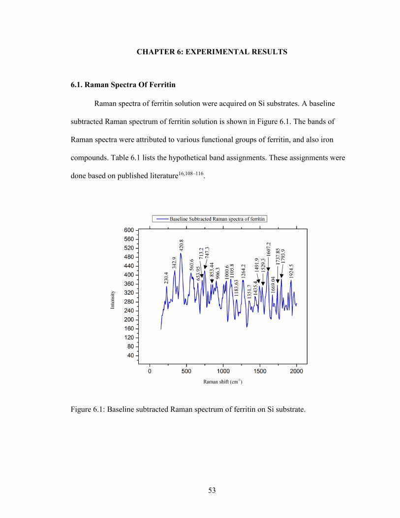
53

CHAPTER 6: EXPERIMENTAL RESULTS

6.1. Raman Spectra Of Ferritin

Raman spectra of ferritin solution were acquired on Si substrates. A baseline

subtracted Raman spectrum of ferritin solution is shown in Figure 6.1. The bands of

Raman spectra were attributed to various functional groups of ferritin, and also iron

compounds. Table 6.1 lists the hypothetical band assignments. These assignments were

done based on published literature16,108–116.

Figure 6.1: Baseline subtracted Raman spectrum of ferritin on Si substrate.

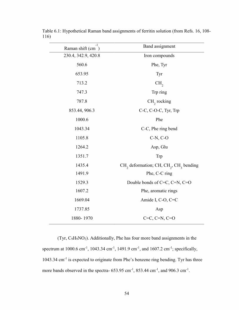
54

Table 6.1: Hypothetical Raman band assignments of ferritin solution (from Refs. 16, 108-

116)

Raman shift (cm-1

) Band assignment

230.4, 342.9, 420.8 Iron compounds

560.6 Phe, Tyr

653.95 Tyr

713.2 CH2

747.3 Trp ring

787.8 CH2 rocking

853.44, 906.3 C-C, C-O-C, Tyr, Trp

1000.6 Phe

1043.34 C-C, Phe ring bend

1105.8 C-N, C-O

1264.2 Asp, Glu

1351.7 Trp

1435.4 CH2 deformation; CH, CH

2, CH

3 bending

1491.9 Phe, C-C ring

1529.3 Double bonds of C=C, C=N, C=O

1607.2 Phe, aromatic rings

1669.04 Amide I, C-O, C=C

1737.85 Asp

1880- 1970 C=C, C=N, C=O

(Tyr, C9H9NO2). Additionally, Phe has four more band assignments in the

spectrum at 1000.6 cm-1, 1043.34 cm-1, 1491.9 cm-1, and 1607.2 cm-1; specifically,

1043.34 cm-1 is expected to originate from Phe’s benzene ring bending. Tyr has three

more bands observed in the spectra- 653.95 cm-1, 853.44 cm-1, and 906.3 cm-1.

55

Tryptophan (Trp, C11H10N2O), has characteristic peaks at 747.3 cm-1, 853.44 cm-1, 906.3

cm-1, and 1351.7 cm-1, where the band at 747.3 cm-1 is assigned to Trp ring. Aspartic acid

(Asp, C4H5NO3) and Glutamic acid (Glu, C5H7NO3) both have Raman bands at 1264.2

cm-1. Additionally, Asp has another Raman band at 1737.85 cm-1. Other Raman peaks, as

indicated in the table, are expected to originate from C, N, and O bonds.

The low-shift bands at 230.4 cm-1, 342.9 cm-1, and 420.8 cm-1 have been

hypothetically attributed to vibrations of Fe–O coordination bonds of iron ions present in

ferritin.

Interestingly, Raman spectra of powdered apo-ferritin without ferrihydrite mineral

on a Si substrate shows similar bands, with some occasional peak shifts or intensity

variations. For example, the peak at 853.44 cm-1, representing C-C, C-O-C, residue Tyr,

and residue Trp, is not present in powdered apo-ferritin. I can see only a very small peak

in that region, whereas in ferritin solution, this peak is well pronounced. Similarly,

Raman band at 1529.3 cm-1 representing vibrations of double bonds is very weak in

powdered apo-ferritin. The Raman band at 1264.2 cm-1 that I attribute to Phe and Glu in

ferritin solution has shifted to 1275.2 cm-1 in powdered ferritin. For residue Phe and

vibrations of aromatic rings, I can also see a shift from 1607.2 cm-1 in ferritin solution to

1614.1 cm-1 in powdered apo-ferritin.

Instead of the three low-shift peaks at 230.4 cm-1, 342.9 cm-1, and 420.8 cm-1 that

have been attributed to iron compounds, in apo-ferritin, I observe three peaks at slightly

different positions, 228.6 cm-1, 341.4 cm-1, and 424.8 cm-1. A possible interpretation is

that the lyophilized powdered ferritin sample still contain some iron ions.

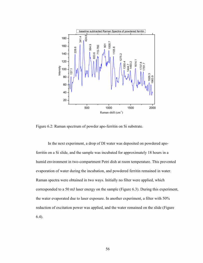
56

Figure 6.2: Raman spectrum of powder apo-ferritin on Si substrate.

In the next experiment, a drop of DI water was deposited on powdered apo-

ferritin on a Si slide, and the sample was incubated for approximately 18 hours in a

humid environment in two-compartment Petri dish at room temperature. This prevented

evaporation of water during the incubation, and powdered ferritin remained in water.

Raman spectra were obtained in two ways. Initially no filter were applied, which

corresponded to a 50 mJ laser energy on the sample (Figure 6.3). During this experiment,

the water evaporated due to laser exposure. In another experiment, a filter with 50%

reduction of excitation power was applied, and the water remained on the slide (Figure

6.4).

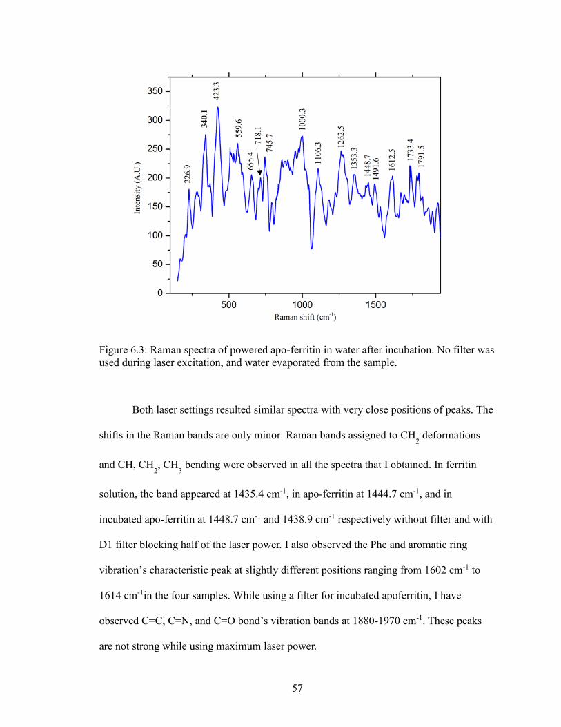
57

Figure 6.3: Raman spectra of powered apo-ferritin in water after incubation. No filter was

used during laser excitation, and water evaporated from the sample.

Both laser settings resulted similar spectra with very close positions of peaks. The

shifts in the Raman bands are only minor. Raman bands assigned to CH2 deformations

and CH, CH2, CH

3 bending were observed in all the spectra that I obtained. In ferritin

solution, the band appeared at 1435.4 cm-1, in apo-ferritin at 1444.7 cm-1, and in

incubated apo-ferritin at 1448.7 cm-1 and 1438.9 cm-1 respectively without filter and with

D1 filter blocking half of the laser power. I also observed the Phe and aromatic ring

vibration’s characteristic peak at slightly different positions ranging from 1602 cm-1 to

1614 cm-1in the four samples. While using a filter for incubated apoferritin, I have

observed C=C, C=N, and C=O bond’s vibration bands at 1880-1970 cm-1. These peaks

are not strong while using maximum laser power.

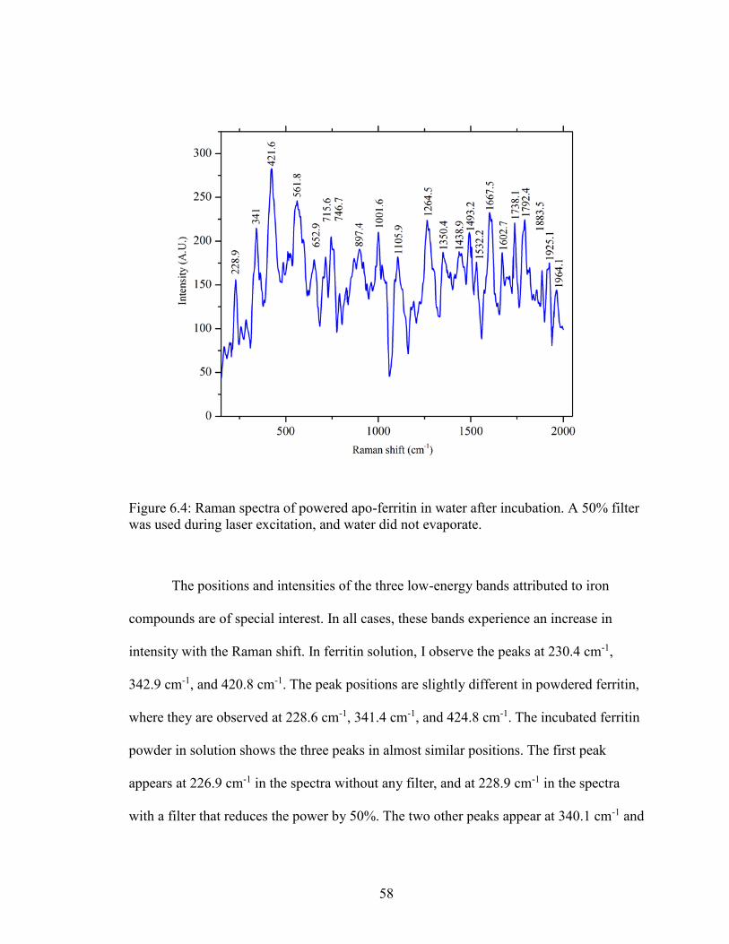
58

Figure 6.4: Raman spectra of powered apo-ferritin in water after incubation. A 50% filter

was used during laser excitation, and water did not evaporate.

The positions and intensities of the three low-energy bands attributed to iron

compounds are of special interest. In all cases, these bands experience an increase in

intensity with the Raman shift. In ferritin solution, I observe the peaks at 230.4 cm-1,

342.9 cm-1, and 420.8 cm-1. The peak positions are slightly different in powdered ferritin,

where they are observed at 228.6 cm-1, 341.4 cm-1, and 424.8 cm-1. The incubated ferritin

powder in solution shows the three peaks in almost similar positions. The first peak

appears at 226.9 cm-1 in the spectra without any filter, and at 228.9 cm-1 in the spectra

with a filter that reduces the power by 50%. The two other peaks appear at 340.1 cm-1 and

59

423.3 cm-1 in the spectra without filter. Applying the filter results in the peaks appearing

at 341 cm-1 and 421.6 cm-1.

6.2. Raman Characterization Of Mohr’s Salt

Mohr’s salt (Ammonium iron (II) sulfate hexahydrate) is a common laboratory

source of iron ions. Raman spectroscopy of Mohr’s salt was performed in order to clarify,

whether the three low-shift bands that were observed in different ferritin samples indeed

should be attributed to iron ions’ bonds with other compounds.

The experiment on Mohr’s salt was done in two ways. In one setup, I used the

powdered Mohr’s salt on a Si substrate, and exposed the sample directly to the laser in

order to acquire the Raman spectrum. In another setup, the Mohr’s salt was incubated in

Petri dish for about 18 hours at room temperature, on a similar Si substrate.

Figure 6.5 depicts a Raman spectrum of powdered Mohr’s salt, and Figure 6.6

shows a Raman spectrum of incubated Mohr’s salt solution. The spectrum of powder

Mohr’s salt exhibits three distinct low-shift bands at 191.9 cm-1, 326.05 cm-1, and 472.09

cm-1, as shown in Figure 6.5. The incubated Mohr’s salt solution shows three low-shift

bands as well, at 183.23 cm-1, 318.2 cm-1, and 462.62 cm-1. Thus, after incubation in

water the bands are observed at lower Raman shifts.

I expect that the described bands originate from Fe-O bond vibrations. Iron oxides

are known to produce low-shift Raman bands below 600 cm-1.113–115 For example,

exposure of Fe3O4 to a 514.5 nm laser light yields a peak116 at 474 cm-1. In my

experiments, I observe a very close peak at 472.09 cm-1 (Figure 6.5) and 462.62 cm-1

(Figure 6.6), in both setups.

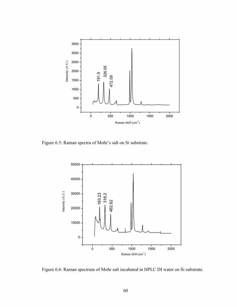
60

Figure 6.5: Raman spectra of Mohr’s salt on Si substrate.

Figure 6.6: Raman spectrum of Mohr salt incubated in HPLC DI water on Si substrate.

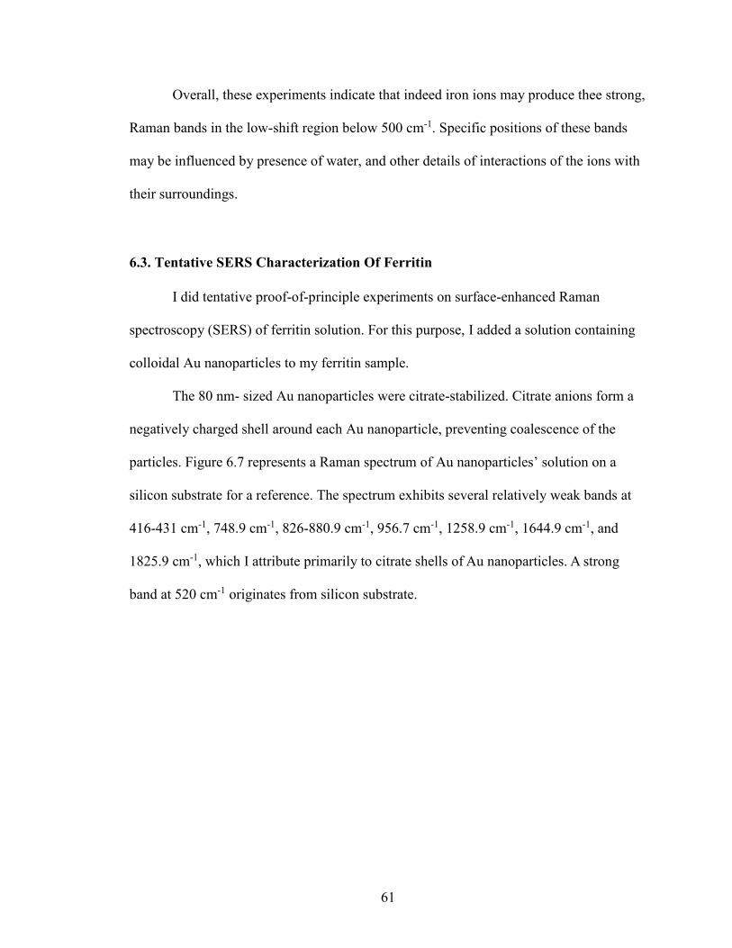
61

Overall, these experiments indicate that indeed iron ions may produce thee strong,

Raman bands in the low-shift region below 500 cm-1. Specific positions of these bands

may be influenced by presence of water, and other details of interactions of the ions with

their surroundings.

6.3. Tentative SERS Characterization Of Ferritin

I did tentative proof-of-principle experiments on surface-enhanced Raman

spectroscopy (SERS) of ferritin solution. For this purpose, I added a solution containing

colloidal Au nanoparticles to my ferritin sample.

The 80 nm- sized Au nanoparticles were citrate-stabilized. Citrate anions form a

negatively charged shell around each Au nanoparticle, preventing coalescence of the

particles. Figure 6.7 represents a Raman spectrum of Au nanoparticles’ solution on a

silicon substrate for a reference. The spectrum exhibits several relatively weak bands at

416-431 cm-1, 748.9 cm-1, 826-880.9 cm-1, 956.7 cm-1, 1258.9 cm-1, 1644.9 cm-1, and

1825.9 cm-1, which I attribute primarily to citrate shells of Au nanoparticles. A strong

band at 520 cm-1 originates from silicon substrate.

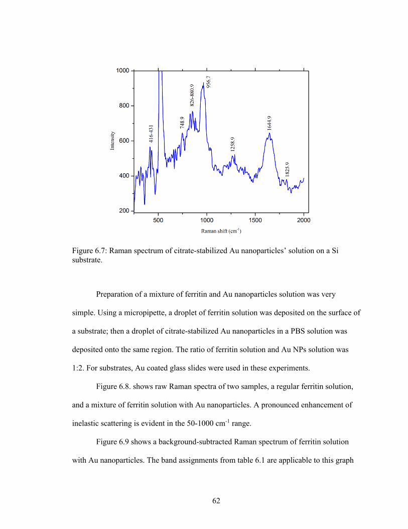
62

Figure 6.7: Raman spectrum of citrate-stabilized Au nanoparticles’ solution on a Si

substrate.

Preparation of a mixture of ferritin and Au nanoparticles solution was very

simple. Using a micropipette, a droplet of ferritin solution was deposited on the surface of

a substrate; then a droplet of citrate-stabilized Au nanoparticles in a PBS solution was

deposited onto the same region. The ratio of ferritin solution and Au NPs solution was

1:2. For substrates, Au coated glass slides were used in these experiments.

Figure 6.8. shows raw Raman spectra of two samples, a regular ferritin solution,

and a mixture of ferritin solution with Au nanoparticles. A pronounced enhancement of

inelastic scattering is evident in the 50-1000 cm-1 range.

Figure 6.9 shows a background-subtracted Raman spectrum of ferritin solution

with Au nanoparticles. The band assignments from table 6.1 are applicable to this graph

63

Figure 6.8: Raw Raman spectra of ferritin solution with Au nanoparticles (red line), and

of regular ferritin solution without nanoparticles (blue line) on Au coated glass substrate.

These spectra were not background-subtracted.

as well. I can see a significant enhancement of the signal in the low-shift part of the

spectrum below 750 cm-1. The three peaks that I tentatively attribute to iron ion

compounds have undergone the strongest enhancement. There is a small peak at 270.5

cm-1, presumably originating from Au nanoparticles, as in Figure 6.7, smaller peaks are

visible around a 250 cm-1 region. However, all major peaks from 550 cm-1 to 1440 cm-1

and from 1600 cm-1 to 1880 cm-1 are very closely positioned to their counterparts in the

Raman spectra of ferritin solution, ferritin powder, and incubated ferritin samples from

Section 6.1.

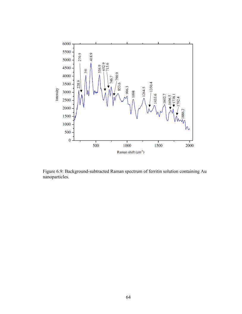
64

Figure 6.9: Background-subtracted Raman spectrum of ferritin solution containing Au

nanoparticles.

65

CHAPTER 7: DISCUSSION

The Raman spectra of ferritin solution acquired in my experiments exhibit three

distinct bands, at 230.4 cm-1, 342.9 cm-1, and 420.8 cm-1. These bands are tentatively

attributed to vibrations of iron ions containing compounds. In iron-loaded ferritin,

vibrations of Fe–O bonds in ferrihydrite nanoparticles are a natural explanation. My

Raman spectrum of Mohr’s salt also contain three low-energy bands in the same region

between approximately 180 cm-1 and 480 cm-1. This supports my interpretation of the

three distinct peaks in ferritin as originating from bonds of iron ions. Interestingly, in my

SERS characterization of ferritin solution containing 80 nm Au nanoparticles, I achieved

a significant enhancement of the iron-associated Raman bands. This indicates a strong

potential of SERS as a method of investigating iron-loaded ferritin.

Surprisingly, the three characteristic bands were also present in Raman spectrum

of apo-ferritin that does not contain ferrihydrite nanoparticles. The bands were observed

in dry apo-ferritin powder, as well as after incubation of the powder in water.

The computational part of my work addresses the mechanism of transit of iron

ions in and out of the ferritin’s cage. my simulations indicate that ions located either side

of ferritin’s three-fold channel quickly enter into the channel in less than 2 ns, due to

electrostatic attraction of negatively charged regions around the channel. In simulations

with iron ions positioned on the outer side of the channel, the second and in one case,

even the third ion entered the channel in the course of only 20 ns. These other ions seem

to expel the first ion out of the channel by electrostatic repulsion. In two simulations out

of the three, the first ion exited from the channel due to repelling action of another iron

ion. In simulations with ions added on the inner side of the channel, one ion entered the

66

channel and remained there. The second ion approached closely, but did not enter the

channel. In one trajectory, two ions approached the channel from inside. However, the

second and third ions did not enter the channel, and the first ion did not exit in any of the

three simulations with ions positioned inside.

In all cases, ions that enter the three-fold channel of ferritin are found in a stable

position, and may remain there for a long time. From electrostatic potential analysis, I

saw that three-fold channels are negatively charged. The positively charged iron ion is

stable surrounded by acidic groups from ferritin’s side chains. For an iron ion to exit from

the channel, it needs a repulsion from second or possibly even third ion. In the absence of

the other ions in the channel, the first ion does not exit.

The described computational results help explain why, in my experiments, apo-

ferritin exhibits three distinct low-shift Raman bands, which are attributable to iron

compounds. I hypothesize that these bands may originate from iron ions caught in, or

closely positioned to three-fold channels of apo-ferritin. my molecular dynamics results

indicate that iron ions in the channel are stable and can remain there for a significant

time.

67

CHAPTER 8: CONCLUSIONS AND FUTURE WORK

8.1. Conclusions

An important cage protein, ferritin, has been investigated both computationally and

experimentally. The following conclusions can be drawn.

• Results of my molecular dynamics simulations suggest that positively charged

iron ions enter the three-fold channel of ferritin spontaneously, driven by

attraction of negatively charged regions around the channel. A second ion, and

sometimes more, were found to approach the channel. Some of these other ions

entered the channel, following the first ion.

• In case of iron ions added outside of the channel, exit of the ion from the inner

opening of the channel was observed. The second ion repeals the first ion toward

its complete expulsion from the channel. The effect of the second ion is critical

for the expulsion of the first one.

• During their travel through the channel, iron ions remain surrounded by water

solvation shells. The first solvation shell is very stable, and the second one

undergoes only minor changes.

• Ion travelling through the channel are found in close proximity of carboxylate

groups from Glu130 residues in the channel area, which attract the ions

electrostatically. Mediation through water molecules seems to play an important

role in this interaction.

• Without expulsion by a second ion, the first ion would remain in the channel.

68

• In my experimental work, Raman spectra of iron-loaded ferritin solution were

obtained. The spectra contain three low-shift Raman bands, which have been

attributed to vibrations of bonds in iron containing compounds.

• Raman spectra of apo-ferritin also exhibited similar low-shift bands. Based on the

results of MD simulations, these bands are thought to originate from interactions

of iron ions in ferritin’s channels.

• Raman characterization of ferritin solution with the addition of colloidal Au

nanoparticles has demonstrated a pronounced Raman signal enhancement in the

low-shift area, promising a strong potential of SERS for characterization of

ferritin.

8.2. Future Work

Investigating interactions of iron ions inside ferritin’s globule is important to

elucidate details of ferritin functionality. The function of iron storage and release of

ferritin can be extended to different nanoparticles storage and release, employing

modified ferritin-like cage proteins. Molecular dynamics case studies of such proteins

will also be useful.

For future works, the author suggests extending molecular dynamics simulations

to even longer time. Also, adding more ions in simulation boxes, while balancing the

charge though negative counterions, may allow observing more than two ions entering in

the channel. Increasing the simulation box size would also be required to decrease the

number of ions per unit volume, in order to observe a complete ion expulsion from the

channel.

69

Raman characterization, on the other hand, could be extended to different

modified ferritins, such as PDB ID 5CZU, which can be synthesized and undergo Raman

or SERS characterization. Modified ferritins may have improved engineered

functionalities. For instance, 5CZU has Sulphur containing side chains in three residues

near the three-fold channel on the outside of the cage. These Sulphur groups may be used

to bind ferritin to gold nanoparticles, enabling an efficient SERS enhancement is

achieved in the region of three-fold channel.

Many applications that use nanoparticles, such as for example cancer therapies,

require transport of caged NPs, making detailed vibrational characterization and

molecular dynamics studies of ferritin and ferritin-like proteins very much important for

future advancement of materials science.

70

REFERENCES

1. Zazo, H., Colino, C. I. & Lanao, J. M. Current applications of nanoparticles in

infectious diseases. Journal of Controlled Release 224, 86–102 (2016).

2. Romo-Herrera, J. M. et al. A study of the depth and size of concave cube Au

nanoparticles as highly sensitive SERS probes. Nanoscale 8, 7326–7333 (2016).

3. Oberdörster, G., Oberdörster, E. & Oberdörster, J. Nanotoxicology: An Emerging

Discipline Evolving from Studies of Ultrafine Particles. Environ. Health Perspect.

113, 823–839 (2005).

4. Lacave, J. M. et al. Effects of metal-bearing nanoparticles (Ag, Au, CdS, ZnO,

SiO 2 ) on developing zebrafish embryos. Nanotechnology 27, 325102 (2016).

5. Salata, O. Applications of nanoparticles in biology and medicine. J.

Nanobiotechnology 2, 3 (2004).

6. Talapin, D. V. & Shevchenko, E. V. Introduction: Nanoparticle chemistry. Chem.

Rev. 116, 10343–10345 (2016).

7. Hoecker, C., Smail, F., Bajada, M., Pick, M. & Boies, A. Catalyst nanoparticle

growth dynamics and their influence on product morphology in a CVD process for

continuous carbon nanotube synthesis. Carbon N. Y. 96, 116–124 (2016).

8. Park, J. et al. Cooperative nanomaterial system to sensitize , target , and treat

tumors. 107, (2010).

9. Desiraju, G. R. The Raman Effect. Nat. India 1–3 (2008).

doi:10.1038/nindia.2008.302

10. Butler, H. J. et al. Using Raman spectroscopy to characterize biological materials.

Nat. Protoc. 11, 664–687 (2016).

11. Zrimsek, A. B. et al. Single-Molecule Chemistry with Surface- and Tip-Enhanced

Raman Spectroscopy. Chem. Rev. acs.chemrev.6b00552 (2016).

doi:10.1021/acs.chemrev.6b00552

12. Kneipp, K., Kneipp, H., Itzkan, I., Dasari, R. R. & Feld, M. S. Surface-Enhanced

Raman Scattering and Biophysics. J. Phys. Condens. Matter Matter 14, R597–

R624 (2002).

13. Stiles, P. L., Dieringer, J. a, Shah, N. C. & Van Duyne, R. P. Surface-enhanced

Raman spectroscopy. Annu. Rev. Anal. Chem. (Palo Alto. Calif). 1, 601–626

(2008).

14. Sergiienko, S., Moor, K., Gudun, K., Elemessova, Z. & Bukasov, R. Nanoparticle-

nanoparticle vs nanoparticle-substrate hot spot contributions to SERS signal:

studying Raman labelled monomers, dimers and trimers. Phys. Chem. Chem. Phys.

19, 4478–4487 (2016).

71

15. Wustholz, K. L. et al. Structure-activity relationships in gold nanoparticle dimers

and trimers for surface-enhanced raman spectroscopy. J. Am. Chem. Soc. 132,

10903–10910 (2010).

16. Xu, L. et al. Label-Free Detection of Native Proteins by Surface-Enhanced Raman

Spectroscopy Using Iodide-Modified Nanoparticles. Anal. Chem. 86, 2238–2245

(2014).

17. Han, X. X., Huang, G. G., Zhao, B. & Ozaki, Y. Label-Free Highly Sensitive

Detection of Proteins in Aqueous Solutions Using Surface-Enhanced Raman

Scattering. Anal. Chem. 81, 3329–3333 (2009).

18. Huang, G. G., Han, X. X., Hossain, M. K. & Osaki, Y. Development of a Heat-

Induced Surface-Enhanced Raman Scattering Sensing Method for Rapid Detection

of Glutathione in Aqueous Solutions. Anal. Chem. 81, 5881–5888 (2009).

19. Kahraman, M., Balz, B. N. & Wachsmann-Hogiu, S. Hydrophobicity-driven self-

assembly of protein and silver nanoparticles for protein detection using surface-

enhanced Raman scattering. Analyst 138, 2906–13 (2013).

20. Israelsen, N. D., Hanson, C. & Vargis, E. Nanoparticle Properties and Synthesis

Effects on Surface-Enhanced Raman Scattering Enhancement Factor: An

Introduction. Sci. World J. 2015, 1–12 (2015).

21. Lyandres, O. et al. Progress toward an in vivo surface-enhanced Raman

spectroscopy glucose sensor. Diabetes Technol. Ther. 10, 257–65 (2008).

22. Yonzon, C. R., Haynes, C. L., Zhang, X., Walsh, J. T. & Van Duyne, R. P. A

Glucose Biosensor Based on Surface-Enhanced Raman Scattering: Improved

Partition Layer, Temporal Stability, Reversibility, and Resistance to Serum Protein

Interference. Anal. Chem. 76, 78–85 (2004).

23. Dendisova-Vyskovska, M., Broncova, G., Clupek, M., Prokopec, V. & Matejka, P.

In situ SERS spectroelectrochemical analysis of antioxidants deposited on copper

substrates: What is the effect of applied potential on sorption behavior?

Spectrochim. Acta - Part A Mol. Biomol. Spectrosc. 99, 196–204 (2012).

24. Podstawka, E., Ozaki, Y. & Proniewicz, L. M. Part III: Surface-enhanced raman

scattering of amino acids and their homodipeptide monolayers deposited onto

colloidal gold surface. Appl. Spectrosc. 59, 1516–1526 (2005).

25. Barhoumi, A., Zhang, D., Tam, F. & Halas, N. J. Surface-enhanced Raman

spectroscopy of DNA. J. Am. … 130, 5523–9 (2008).

26. Cui, Y. et al. Au@organosilica multifunctional nanoparticles for the multimodal

imaging. Chem. Sci. 2, 1463–1469 (2011).

27. Qian, X. et al. In vivo tumor targeting and spectroscopic detection with surface-

enhanced Raman nanoparticle tags. Nat. Biotechnol. 26, 83–90 (2008).

28. Pallaoro, A., Hoonejani, M. R., Braun, G. B., Meinhart, C. D. & Moskovits, M.

Rapid identification by surface-enhanced raman spectroscopy of cancer cells at

72

low concentrations flowing in a microfluidic channel. ACS Nano 9, 4328–4336

(2015).

29. Lin, D. et al. Label-free detection of blood plasma using silver nanoparticle based

surface-enhanced Raman spectroscopy for esophageal cancer screening. J.

Biomed. Nanotechnol. 10, 478–484 (2014).

30. Yang, J. et al. Surface-enhanced Raman spectroscopy based quantitative bioassay

on aptamer-functionalized nanopillars using large-area Raman mapping. ACS

Nano 7, 5350–5359 (2013).

31. MaHam, A., Tang, Z., Wu, H., Wang, J. & Lin, Y. Protein-Based Nanomedicine

Platforms for Drug Delivery. Small 5, 1706–1721 (2009).

32. Bantz, K. C. et al. Recent progress in SERS biosensing. Phys. Chem. Chem. Phys.

13, 11551–67 (2011).

33. Wang, Y., Lee, K. & Irudayaraj, J. SERS aptasensor from nanorod–nanoparticle

junction for protein detection. Chem. Commun. 46, 613–615 (2010).

34. Han, X. X., Zhao, B. & Ozaki, Y. Surface-enhanced Raman scattering for protein

detection. Analytical and Bioanalytical Chemistry 394, 1719–1727 (2009).

35. Hildebrandt, P. & Stockburger, M. Surface-enhanced resonance Raman

spectroscopy of Rhodamine 6G adsorbed on colloidal silver. J. Phys. Chem. 88,

5935–5944 (1984).

36. Xu, T. et al. Enhanced Raman scattering assisted by ultrahigh order modes of the

double metal cladding waveguide. Appl. Phys. Lett. 105, 163703 (2014).

37. Rodríguez-Torres, M. del P., Díaz-Torres, L. A. & Romero-Servin, S. Heparin

assisted photochemical synthesis of gold nanoparticles and their performance as

SERS substrates. Int. J. Mol. Sci. 15, 19239–19252 (2014).

38. Rowland, C. E., Brown, C. W., Delehanty, J. B. & Medintz, I. L. Nanomaterial-

based sensors for the detection of biological threat agents. Mater. Today 19, 464–

477 (2016).

39. Bell, S. E. J. & Sirimuthu, N. M. S. Surface-Enhanced Raman Spectroscopy

(SERS) for Sub-Micromolar Detection of DNA/RNA Mononucleotides. J. Am.

Chem. Soc. 128, 15580–15581 (2006).

40. Pincella, F., Isozaki, K. & Miki, K. A visible light-driven plasmonic photocatalyst.

Light Sci. Appl. 3, e133 (2014).

41. Delga, A., Feist, J., Bravo-Abad, J. & Garcia-Vidal, F. J. Theory of strong

coupling between quantum emitters and localized surface plasmons. J. Opt. 16,

114018 (2014).

42. Guarrotxena, N. & Bazan, G. C. Antitags: SERS-encoded nanoparticle assemblies

that enable single-spot multiplex protein detection. Adv. Mater. 26, 1941–1946

(2014).

73

43. Han, X. X. et al. Protein-mediated sandwich strategy for surface-enhanced raman

scattering: Application to versatile protein detection. Anal. Chem. 81, 3350–3355

(2009).

44. Lim, D.-K. et al. Highly uniform and reproducible surface-enhanced Raman

scattering from DNA-tailorable nanoparticles with 1-nm interior gap. Nat.

Nanotechnol. 6, 452–460 (2011).

45. Feng, M. & Tachikawa, H. Surface-enhanced resonance Raman spectroscopic

characterization of the protein native structure. J. Am. Chem. Soc. 130, 7443–7448

(2008).

46. Bernardi, R. C., Melo, M. C. R. & Schulten, K. Enhanced sampling techniques in

molecular dynamics simulations of biological systems. Biochim. Biophys. Acta

1850, 872–877 (2015).

47. Perilla, J. R. et al. Molecular dynamics simulations of large macromolecular

complexes. Current Opinion in Structural Biology 31, 64–74 (2015).

48. Malmstrom, R. D., Lee, C. T., Van Wart, A. T. & Amaro, R. E. Application of

molecular-dynamics based markov state models to functional proteins. J. Chem.

Theory Comput. 10, 2648–2657 (2014).

49. Han, Y. & Elliott, J. Molecular dynamics simulations of the elastic properties of

polymer/carbon nanotube composites. Comput. Mater. Sci. 39, 315–323 (2007).

50. Karplus, M. & McCammon, J. A. Molecular dynamics simulations of

biomolecules. Nat. Struct. Biol. 9, 646–652 (2002).

51. MacKerell, A. D. & Banavali, N. K. All-atom empirical force field for nucleic

acids: II. Application to molecular dynamics simulations of DNA and RNA in

solution. J. Comput. Chem. 21, 105–120 (2000).

52. Wilfred, B., Gunsteren, V. & Berendsen, C. Computer Simulation of Molecular

Dynamics: Methodology, Applications, and Perspectives in Chemistry. Anger,.

Chem. lnr. Ed. Engl 29, 992–1023 (1990).

53. Sankey, O. F. & Niklewski, D. J. Ab initio multicenter tight-binding model for

molecular-dynamics simulations and other applications in covalent systems. Phys.

Rev. B 40, 3979–3995 (1989).

54. Miao, Y. et al. Improved reweighting of accelerated molecular dynamics

simulations for free energy calculation. J. Chem. Theory Comput. 10, 2677–2689

(2014).

55. Simonson, T., Archontis, G. & Karplus, M. Free Energy Simulations Come of

Age: Protein−Ligand Recognition. Acc. Chem. Res. 35, 430–437 (2002).

56. Humphrey, W., Dalke, A. & Schulten, K. VMD: Visual molecular dynamics. J.

Mol. Graph. 14, 33–38 (1996).

57. Karplus, M. Molecular dynamics of biological macromolecules: A brief history

74

and perspective. in Biopolymers 68, 350–358 (2003).

58. Kumar, A. & Purohit, R. Use of Long Term Molecular Dynamics Simulation in

Predicting Cancer Associated SNPs. PLoS Comput. Biol. 10, (2014).

59. Laghaei, R., Kowallis, W., Evans, D. G. & Coalson, R. D. Calculation of iron

transport through human H-chain ferritin. J. Phys. Chem. A 118, 7442–7453

(2014).

60. Chandramouli, B., Bernacchioni, C., Di Maio, D., Turano, P. & Brancato, G.

Electrostatic and Structural Bases of Fe2+ Translocation Through Ferritin

Channels. J. Biol. Chem. M116.748046- (2016). doi:10.1074/jbc.M116.748046

61. Laghaei, R., Evans, D. G. & Coalson, R. D. Metal binding sites of human H-chain

ferritin and iron transport mechanism to the ferroxidase sites: A molecular

dynamics simulation study. Proteins Struct. Funct. Bioinforma. 81, 1042–1050

(2013).

62. Honarmand Ebrahimi, K., Hagedoorn, P.-L. & Hagen, W. R. Unity in the

Biochemistry of the Iron-Storage Proteins Ferritin and Bacterioferritin. Chem. Rev.

115, 295–326 (2015).

63. Nakajima, H. et al. Construction of an enterobactin analogue with symmetrically

arranged monomer subunits of ferritin. Chem. Commun. 51, 16609–16612 (2015).

64. Schrödinger, LLC. The {PyMOL} Molecular Graphics System, Version~1.8.

(2015).

65. Jutz, G., van Rijn, P., Santos Miranda, B. & Böker, A. Ferritin: A Versatile

Building Block for Bionanotechnology. Chem. Rev. 115, 1653–1701 (2015).

66. MULLER, R. N. et al. RELAXATION BY METAL-CONTAINING

NANOSYSTEMS. Advances in Inorganic Chemistry 57, 239–292 (2006).

67. Schrödinger, LLC. The {JyMOL} Molecular Graphics Development Component,

Version~1.8. (2015).

68. Kasyutich, O. et al. Silver Ion Incorporation and Nanoparticle Formation inside the

Cavity of Pyrococcus furiosus Ferritin: Structural and Size-Distribution Analyses.

J. Am. Chem. Soc. 132, 3621–3627 (2010).

69. May, C. A. et al. The sedimentation properties of ferritins. New insights and

analysis of methods of nanoparticle preparation. Biochim. Biophys. Acta - Gen.

Subj. 1800, 858–870 (2010).

70. Polanams, J., Ray, A. D. & Watt, R. K. Nanophase Iron Phosphate, Iron Arsenate,

Iron Vanadate, and Iron Molybdate Minerals Synthesized within the Protein Cage

of Ferritin. Inorg. Chem. 44, 3203–3209 (2005).

71. Bedwell, G. J. et al. Selective Biotemplated Synthesis of TiO2 Inside a Protein

Cage. Biomacromolecules 16, 214–218 (2015).

72. Douglas, T. & Young, M. Host-guest encapsulation of materials by assembled

75

virus protein cages. Nature 393, 152–155 (1998).

73. Kang, S. et al. Implementation of P22 Viral Capsids as Nanoplatforms.

Biomacromolecules 11, 2804–2809 (2010).

74. Steinmetz, N. F. Viral Nanoparticles in Drug Delivery and Imaging. Mol. Pharm.

10, 1–2 (2013).

75. Molino, N. M. & Wang, S. W. Caged protein nanoparticles for drug delivery.

Curr. Opin. Biotechnol. 28, 75–82 (2014).

76. Farokhzad, O. C. & Langer, R. Impact of Nanotechnology on Drug Delivery. ACS

Nano 3, 16–20 (2009).

77. Wagner, V., Dullaart, A., Bock, A.-K. & Zweck, A. The emerging nanomedicine

landscape. Nat Biotech 24, 1211–1217 (2006).

78. Yildiz, I., Shukla, S. & Steinmetz, N. F. Applications of viral nanoparticles in

medicine. Curr. Opin. Biotechnol. 22, 901–908 (2011).

79. Uchida, M. et al. Biological Containers: Protein Cages as Multifunctional

Nanoplatforms. Adv. Mater. 19, 1025–1042 (2007).

80. Smith, M. T., Hawes, A. K. & Bundy, B. C. Reengineering viruses and virus-like

particles through chemical functionalization strategies. Curr. Opin. Biotechnol. 24,

620–626 (2013).

81. Aljabali, A. A. A., Shukla, S., Lomonossoff, G. P., Steinmetz, N. F. & Evans, D. J.

CPMV-DOX Delivers. Mol. Pharm. 10, 3–10 (2013).

82. Moon, H., Lee, J., Min, J. & Kang, S. Developing Genetically Engineered

Encapsulin Protein Cage Nanoparticles as a Targeted Delivery Nanoplatform.

Biomacromolecules 15, 3794–3801 (2014).

83. Berendsen, H. J. C., van der Spoel, D. & van Drunen, R. GROMACS: A message-

passing parallel molecular dynamics implementation. Comput. Phys. Commun. 91,

43–56 (1995).

84. Lindahl, E., Hess, B. & Spoel, D. Van Der. GROMACS 3 . 0 : a package for

molecular simulation and trajectory analysis. J. Mol. Model. 306–317 (2001).

doi:10.1007/s008940100045

85. Van Der Spoel, D. et al. GROMACS: Fast, flexible, and free. J. Comput. Chem.

26, 1701–1718 (2005).

86. Hess, B., Kutzner, C., van der Spoel, D. & Lindahl, E. GROMACS 4: Algorithms

for Highly Efficient, Load-Balanced, and Scalable Molecular Simulation. J. Chem.

Theory Comput. 4, 435–447 (2008).

87. Pronk, S. et al. GROMACS 4.5: a high-throughput and highly parallel open source

molecular simulation toolkit. Bioinformatics 29, 845 (2013).

88. Páll, S., Abraham, M. J., Kutzner, C., Hess, B. & Lindahl, E. in (eds. Markidis, S.

76

& Laure, E.) 3–27 (Springer International Publishing, 2015). doi:10.1007/978-3-

319-15976-8_1

89. Abraham, M. J. et al. Gromacs: High performance molecular simulations through

multi-level parallelism from laptops to supercomputers. SoftwareX 1–2, 19–25

(2015).

90. Van Gunsteren, F. W. et al. Biomolecular Simulation: The GROMOS96 Manual

and User Guide. Biomolecular Simulation: The GROMOS96 Manual and User

Guide (1996). doi:citeulike-article-id:8062915

91. Oostenbrink, C., Villa, A., Mark, A. E. & Van Gunsteren, W. F. A biomolecular

force field based on the free enthalpy of hydration and solvation: The GROMOS

force-field parameter sets 53A5 and 53A6. J. Comput. Chem. 25, 1656–1676

(2004).

92. Jorgensen, W. L., Maxwell, D. S. & Tirado-Rives, J. Development and Testing of

the OPLS All-Atom Force Field on Conformational Energetics and Properties of

Organic Liquids. J. Am. Chem. Soc. 118, 11225–11236 (1996).

93. Kaminski, G. A., Friesner, R. A., Tirado-Rives, J. & Jorgensen, W. L. Evaluation

and Reparametrization of the OPLS-AA Force Field for Proteins via Comparison

with Accurate Quantum Chemical Calculations on Peptides. J. Phys. Chem. B 105,

6474–6487 (2001).

94. Brooks, B. R. et al. CHARMM: The biomolecular simulation program. J. Comput.

Chem. 30, 1545–1614 (2009).

95. Case, D. A. et al. The Amber biomolecular simulation programs. J. Comput.

Chem. 26, 1668–1688 (2005).

96. Hess, B., Spoel, D. van der & Lindahl, E. Gromacs User Manual. Dep. Biophys.

Chem. … 312 (2014). doi:10.1006/imms.1993.1022

97. Berendsen, H. J. C., Postma, J. P. M., van Gunsteren, W. F. & Hermans, J. in

Intermolecular Forces: Proceedings of the Fourteenth Jerusalem Symposium on

Quantum Chemistry and Biochemistry Held in Jerusalem, Israel, April 13--16,

1981 (ed. Pullman, B.) 331–342 (Springer Netherlands, 1981). doi:10.1007/978-

94-015-7658-1_21

98. Li, P., Roberts, B. P., Chakravorty, D. K. & Merz, K. M. Rational design of

particle mesh ewald compatible lennard-jones parameters for +2 metal cations in

explicit solvent. J. Chem. Theory Comput. 9, 2733–2748 (2013).

99. Bussi, G., Donadio, D. & Parrinello, M. Canonical sampling through velocity

rescaling. J. Chem. Phys. 126, (2007).

100. Nosé, S. & Klein, M. L. Constant pressure molecular dynamics for molecular

systems. Mol. Phys. 50, 1055–1076 (1983).

101. Parrinello, M. & Rahman, A. Polymorphic transitions in single crystals: A new

molecular dynamics method. J. Appl. Phys. 52, 7182–7190 (1981).

77

102. Hess, B., Bekker, H., Berendsen, H. J. C. & Fraaije, J. G. E. M. LINCS: A Linear

Constraint Solver for Molecular Simulations. J. Comput. Chem 18, 18–1463

(1997).

103. Miyamoto, S. & Kollman, P. A. Settle: An analytical version of the SHAKE and

RATTLE algorithm for rigid water models. J. Comput. Chem. 13, 952–962 (1992).

104. Mathews, N. VMD User ’ s Guide. Methods 51, 1581 (2009).

105. Caddigan, E., Cohen, J., Gullingsrud, J. & Stone, J. VMD User’s Guide. Urbana

51, 61801 (2003).

106. Frishman, D. & Argos, P. Knowledge???based protein secondary structure

assignment. Proteins Struct. Funct. Bioinforma. 23, 566–579 (1995).

107. PDB2PQR Server. doi:http://nbcr-222.ucsd.edu/pdb2pqr_2.1.1/

108. Rygula, A. et al. Raman spectroscopy of proteins: A review. Journal of Raman

Spectroscopy 44, 1061–1076 (2013).

109. Kurouski, D., Postiglione, T., Deckert-Gaudig, T., Deckert, V. & Lednev, I. K.

Amide I vibrational mode suppression in surface (SERS) and tip (TERS) enhanced

Raman spectra of protein specimens. Analyst 138, 1665 (2013).

110. Barth, A. Infrared spectroscopy of proteins. Biochimica et Biophysica Acta -

Bioenergetics 1767, 1073–1101 (2007).

111. Tuma, R. Raman spectroscopy of proteins: from peptides to large assemblies. J.

Raman Spectrosc. 36, 307–319 (2005).

112. Barth, A. & Zscherp, C. What vibrations tell about proteins. Q. Rev. Biophys. 35,

S0033583502003815 (2002).

113. Fan, F., Feng, Z. & Li, C. UV Raman Spectroscopic Studies on Active Sites and

Synthesis Mechanisms of Transition Metal-Containing Microporous and

Mesoporous Materials. Acc. Chem. Res. 43, 378–387 (2010).

114. Chourpa, I. et al. Molecular composition of iron oxide nanoparticles{,} precursors

for magnetic drug targeting{,} as characterized by confocal Raman

microspectroscopy. Analyst 130, 1395–1403 (2005).

115. Li, C. Identifying the isolated transition metal ions/oxides in molecular sieves and

on oxide supports by UV resonance Raman spectroscopy. J. Catal. 216, 203–212

(2003).

116. Mitchell, E. et al. Probing on the hydrothermally synthesized iron oxide

nanoparticles for ultra-capacitor applications. Powder Technol. 272, 295–299

(2015).

study of iron ion transit through three-fold channel of

Documents