study of the 2d heaving and pitching airfoil case using
TRANSCRIPT
Study of the 2D heaving and pitching airfoil case using theSpectral Difference method
by
Caleb Yow, Bin Zhang, Chunlei Liang
Department of Mechanical and Aerospace EngineeringGeorge Washington University
Washington DC, 20052Phone: (202) 994-7073
3rd International Workshop on High-Order CFD Methods
Sponsored by NASA, AIAA, DLR, and Army Research Office (ARO)January 3-4, 2015
at the 53th AIAA Aerospace Sciences Meeting, Kissimmee, Florida
1 Code description
1.1 SD Method
Using the 2D spectral difference (SD) code published in [1] and [2] to handle moving anddeformable grids similar to method reported in [3], Case Study 2.3 was analyzed with a thirdorder SD method. In the SD code, the solution points and flux points are staggered within thegrid in order to achieve the higher order.
The flow field within each cell is reconstructed with a smooth representation using a tensor-product form. The discontinuity across cell interfaces is handled using a Rusanov flux (LocalLax Friedrichs method). We also implemented a p-multigrid scheme for this solver. For thisabstract, all results are obtained using a single-level grid with the 3rd-order SD method.
Consider the following conservative form of the 2D unsteady conservation laws:
∂Q
∂t+∂F
∂x+∂G
∂y=∂Q
∂t+∇Finv(Q)−∇Fv(Q,∇Q) = 0 (1)
where Q is the vector of conserved variables, and F and G are the total fluxes including bothinviscid and viscous flux vectors.

Consider only compressible Navier-Stokes equations, the conservative variables Q and Carte-sian components finv(Q) and ginv(Q) of the inviscid flux vector Finv(bfQ) are given by
Q =
ρρuρvE
, finv(Q) =
ρu
ρu2 + pρuv
u(E + p)
, ginv(Q) =
ρvρuv
ρv2 + pv(E + p)
(2)
where ρ is the density, u and v are the velocity components in x and y directions, p stands forpressure and E is the total energy. The pressure is related to the total energy by
E =p
γ − 1+
1
2ρ(u2 + v2) (3)
with a constant ratio of specific heat γ set as 1.4 for air.The Cartesian components fv(Q,∇Q) and gv(Q,∇Q) of viscous flux vector Fv(Q,∇Q) are
given by
fv = µ
0
2ux + λ(ux + vy)vx + uy
u · fv[2] + v · fv[3] +Cp
PrTx
, gv = µ
0
vx + uy2vy + λ(ux + vy)
u · gv[2] + v · gv[3] +Cp
PrTy
where µ is the dynamic viscosity, Cp is the specific heat and Pr stands for Prandtl number. T istemperature which can be derived from the perfect gas assumption. λ is set to −2/3 accordingto the Stokes hypothesis.
To achieve an efficient implementation, all quadrilateral elements in the moving and de-formable physical domain (x, y, t) are transformed into a square element (0 ≤ ξ ≤ 1, 0 ≤ η ≤ 1,τ = t) as shown in figure 1. The governing equations in the physical domain are then transferredinto the computational domain, and the transformed equations are written as:
∂Q
∂τ+∂F
∂ξ+∂G
∂η= 0 (4)
where[F G Q
]T= |J |J −1
[F G Q
]T. The Jacobian matrix is given by
J =∂(x, y, t)
∂(ξ, η, τ)=
xξ xη xτyξ yη yτ0 0 1
, (5)
where tξ = 0, tη = 0, and t = τ .In the standard element, two sets of points are defined, namely the solution points and
the flux points, as illustrated in figure 1 (b) for a computational cell. A bilinear mapping isemployed to map individual physical cells shown in Fig. 1 (a) to this standard computationalcell.
In order to construct a degree (N − 1) polynomial in each coordinate direction, N solutionpoints are required. The solution points in 1D are chosen to be the Chebyshev-Gauss points.The flux points Xs+1/2 are selected as the Legendre-Gauss-quadrature points plus the two endpoints, 0 and 1, as suggested by following [4] and [5].
Using the solutions at N solution points, a degree (N−1) polynomial can be built using thefollowing Lagrange basis of hi (X). Similarly, using the fluxes at (N + 1) flux points, a degreeN polynomial can be built for the flux using a similar Lagrange basis of li+1/2 (X).
The reconstructed solution for the conserved variables in the standard element is just thetensor products of the two one-dimensional polynomials. The reconstructed flux polynomials are
2

Figure 1: Physical cells and computational cell.
treated in ξ, and η directions as 1D element-wise continuous functions, but discontinuous acrosscell interfaces. For the inviscid flux, a Riemann solver is employed to compute a common fluxat interfaces to ensure conservation and stability. For the viscous flux, an averaging procedureis used.
For dynamic grids considered here, we reformulate the Rusanov solver for the ξ direction as
F inv =1
2
{F invL + F invR − (
∣∣V n
∣∣+ c) · (QR −QL) · |J∇ξ| · s}, (6)
where s is the sign of n · ∇ξ, Vn is the fluid velocity normal to edge interface and c is the speedof sound. For the η direction, it is formulated similarly.
In addition, we must consider geometric conservation law for deforming grid cells:
∂|J |∂τ
+∂(|J |ξt)∂ξ
+∂(|J |ηt)∂η
= 0 (7)
The final compact form after taking into account of the geometric conservation law is givenby
∂Q
∂τ=
1
|J |
{Q
[∂(|J |ξt)∂ξ
+∂(|J |ηt)∂η
]−
[∂F
∂ξ+∂G
∂η
]}. (8)
Equation 8 has a compact form on the computational domain. It offers great ease in handlingmoving and deformable physical domain as well as parallel computation.
1.2 Time marching scheme
All preliminary computations in this abstract utilize a fourth-order accurate, strong-stability-preserving five-stage Runge-Kutta scheme [6].
3

1.3 Parallel Capability
The code is MPI parallelized and can run on an arbitrary number of cores. For this case study,the code was run on 8 processors. The following shows the spacial partitioning:
Figure 2: Partition zones for the 8 processors
1.4 Post-Processing
The post-processing for this case includes computation of the total work W and the verticalimpulse I from that the fluid exerts on the airfoil, these two quantities are defined as below:
W =
∫ 1
0fy(t)h(t)dt+
∫ 1
0Tz(t)θ(t)dt (9)
I =
∫ 1
0fy(t)dt, (10)
where fy is the vertical force, h(t) is the vertical displacement, Tz is the torque about theorigin, and θ(t) is the pitching angle rate of change in radians per second.
2 Case summary
Case C2.3 is investigated in this report. In this case, an initially stationary airfoil starts pitchingand heaving after the surrounding flow reached a steady state. The pitching and heaving lastfor one period, and we are interested in the total work and the vertical impulse that the fluidexerts on the airfoil. Four separate sub-cases were run to establish the effects of changing theSD order and Reynolds number:
• 3rd order Spectral Difference, Re = 1, 000
4

• 3rd order Spectral Difference, Re = 5, 000
• 5th order Spectral Difference, Re = 1, 000
• 5th order Spectral Difference, Re = 5, 000
The SD method is used for the spatial discretization and an explicit five-stage Runge- Kuttascheme is used for the temporal.The time step is set to 5× 10⁻⁵ in all four sub-cases.
The machine used for this test case was a multicore Intel Xeon X5680. Eight of these coreswere used for all calculations. For the first 1,000 iterations of the pitching/heaving calculationat a Reynolds number of 5,000 and N = 5, the computation time was 237.9 seconds per core.At N = 3, this computation time was reduced to 86.05 seconds per core.
3 Meshes
For all sub-cases, the grid space was 200x200 chord lengths with the center of the airfoil locatedat (0,0). The unstructured grid of quadrilateral cells is shown in Fig. 3 (a). The mesh has12,670 cells in all. It employs 60 cells along either top or bottom half surface of the NACA0012airfoil.
(a) Global view of the computational mesh. (b) Close view of the computational mesh.
Figure 3: Mesh
The inflow boundary is 80 chord lengths away from the airfoil center. The top and bottomboundaries are 100 chord lengths from the center, where the inviscid wall boundary condition isadopted. The outflow flow boundary is located 120 chord lengths away from the airfoil center.
The curved surfaces of the airfoil are handled using a cubic spline fitting. Subsequently,the elements adjacent to the surfaces are mapped to a standard square element with 20 nodalpoints via a cubic-order mapping.
During the pitching and heaving motion of the airfoil, the grid is deformed by using ablending function. The exact region of the grid that deforms is an annulus with an internalradius of 5 chord lengths and an external radius of 27 chord lengths.
4 Results
The lift and drag forces of airfoil are normalized using ρu2∞C where C is the chord of the theairfoil which is unity in this case.
5

The SD code was specifically modified for this case study to track the work for these testcases. The vertical work is calculated by adding a summation of all of the viscous and pressure-based vertical forces at all the airfoil solution points at each iteration. The vertical work isfound using
ywork(t) = ywork(t− 1) + h(t) ·∆t · cltot ·1
2ρ∞ · u2∞, (11)
where h(t) is the rate of change of the height of the center of the airfoil, ∆t is the time step,and cltot is the total lift coefficient.
The torsional work is similarly integrated at each solution point by calculating the viscousand pressure-based moments about the origin by using
Tqwork(t) =n∑i=1
[Tqwork(t− 1) + (∆x · Fy + ∆Y · Fx) · θ(t)]n, (12)
where ∆X is the orthogonal distance in the x direction from the current solution pointto the origin, Fy is vertical component of the viscous and pressure-based forces, ∆Y is theorthogonal distance in the y direction from the current solution point to the origin, Fx ishorizontal component of the viscous and pressure-based forces, and θ is the time rate of changeof the angle of the airfoil.
The vertical impulse is calculated as shown in Equation 10 in post-processing in order toreduce the iterative computations.
4.1 Case N=3, Re = 1000
Using a 3rd Order SD method and a Reynolds Number of 1,000, the airfoil followed the pre-scribed pitching and heaving motion after steady-state was achieved. The following Machcontour plots depict the flow fields at t = 0 and t = 1.
Shown below are the mach number contour plots for t=0 and t=1.
6

Figure 4: Mach number contour plot at t=0
Figure 5: Mach number contour plot at t=1
Using the work and impulse equations as shown, the following results were achieved for thisparticular sub-case:
7

Vertical Work Torsional Work Total Work Vertical Impulse
-2.6267937385 -0.9057869362 -3.5325806747 -2.1514975345
4.2 Case N=3, Re = 5000
Using a 3rd Order SD method and a Reynolds Number of 5,000, the airfoil followed the pre-scribed pitching and heaving motion after steady-state was achieved. The following Machcontour plots depict the flow fields at t = 0 and t = 1.
Shown below are the mach number contour plots for t=0 and t=1.
Figure 6: Mach number contour plot at t=0
8

Figure 7: Mach number contour plot at t=1
Using the work and impulse equations as shown, the following results were achieved for thisparticular sub-case:
Vertical Work Torsional Work Total Work Vertical Impulse
-2.6568564138 -1.0273264205 -3.6841828343 -2.2056563772
4.3 Case N=5, Re = 1000
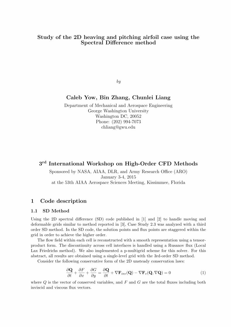
Using a 5th Order SD method and a Reynolds Number of 1,000, the airfoil followed the pre-scribed pitching and heaving motion after steady-state was achieved. The following Machcontour plots depict the flow fields at t = 0 and t = 1.
Shown below are the mach number contour plots for t=0 and t=1.
9
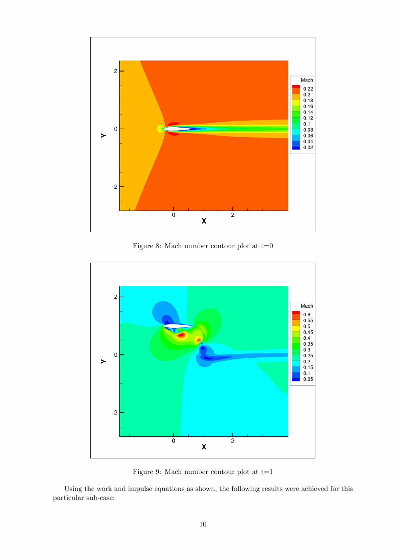
Figure 8: Mach number contour plot at t=0
Figure 9: Mach number contour plot at t=1
Using the work and impulse equations as shown, the following results were achieved for thisparticular sub-case:
10

Vertical Work Torsional Work Total Work Vertical Impulse
-2.6265443136 -0.9069343116 -3.5334786252 -2.1476921744
4.4 Case N=5, Re = 5000
Using a 5th Order SD method and a Reynolds Number of 5,000, the airfoil followed the pre-scribed pitching and heaving motion after steady-state was achieved. The following Machcontour plots depict the flow fields at t = 0 and t = 1.
Shown below are the mach number contour plots for t=0 and t=1.
Figure 10: Mach number contour plot at t=0
11

Figure 11: Mach number contour plot at t=1
Using the work and impulse equations as shown, the following results were achieved for thisparticular sub-case:
Vertical Work Torsional Work Total Work Vertical Impulse
-2.716644523 -0.9956179771 -3.7122625001 -2.2001305479
4.5 Conclusion
The results presented above are tabulated below:
Reynolds Number Order Total Work Vertical Impulse
1,000 3 -3.5325806747 -2.15149753451,000 5 -3.5334786252 -2.14769217445,000 3 -3.6841828343 -2.20565637725,000 5 -3.7122625001 -2.2001305479
From these results, it can be seen that increasing the order from N = 3 to N = 5 producesonly small changes in the calculated variables while increasing the computation time by a factorof 2.8. At Re = 1, 000 increasing the order from N = 3 to N = 5 changed the calculated verticalimpulse by -0.1769% and the total work by 0.0254%. At Re = 5, 000 increasing the order fromN = 3 to N = 5 changed the calculated vertical impulse by -0.2505% and the total work by0.762%.
For reference, the lift and drag coefficients from the dynamic tests are also presented below.From these figures, it can be seen that the results from the 3rd and fifth order calculations
show similar results.
12

Figure 12: Lift Coefficients for all sub-cases
Figure 13: Drag Coefficients for all sub-cases
References
[1] C. Liang, K. Ou, S. Premasuthan, A. Jameson, and Z. J. Wang. High-order accuratesimulations of unsteady flow past plunging and pitching airfoils. Computers and Fluids,
1

40:236–248, 2011.
[2] C. Liang, A. Jameson, and Z. J. Wang. Spectral difference method for two-dimensionalcompressible flow on unstructured grids with mixed elements. Journal of ComputationalPhysics, 228:2847–2858, 2009.
[3] M. L. Yu, Z. J. Wang, and H. Hu. A high-order spectral difference method for unstructureddynamic grids. Computers and Fluids, 48(1):84 – 97, 2011.
[4] K. Van den Abeele, C. Lacor, and Z. J. Wang. On the stability and accuracy of the spectraldifference method. J. of Scientific Computing, 37:162–188, 2008.
[5] H.T. Huynh. A flux reconstruction approach to high-order schemes including discontinuousGalerkin methods. AIAA Paper, AIAA-2007-4079, 2007.
[6] R. J. Spiteri and S. J. Ruuth. A new class of optimal high-order strong-stability-preservingtime discretization methods. SIAM J. Numer. Anal., 40:469–491, 2002.
2