study of the damping and vibration behaviour of flax-carbon composite bicycle racing frames
TRANSCRIPT
Study of the damping and vibration behaviourof flax-carbon composite bicycle racingframes
Joachim Vanwalleghem
Promotoren: prof. dr. ir. Wim Van Paepegem , prof. dr. ir. Mia LoccufierBegeleiders: dr. ir. Ives De Baere, Fangio Reybrouck
Masterproef ingediend tot het behalen van de academische graad vanMaster in de ingenieurswetenschappen: Werktuigkunde-Elektrotechniek
Vakgroep Toegepaste materiaalwetenschappenVoorzitter: prof. dr. ir. Joris Degrieck
Vakgroep Elektrische energie, systemen en automatiseringVoorzitter: prof. dr. ir. Jan Melkebeek
Faculteit IngenieurswetenschappenAcademiejaar 2009–2010
Preface
Een masterproef schrijven doe je niet alleen . . . maar gebeurt met de hulp van andere personen.
Deze wil ik alvast allemaal hartelijk bedanken.
In de eerste plaats wil ik mijn naaste begeleiders bedanken, dit zijn prof. Wim Van Paepegem,
prof. Mia Loccufier, dr. Ives De Baere en Fangio Reybrouck van Museeuw Bikes. Samen met
hen werd er een team gevormd waarbij alle neuzen in dezelfde richting stonden, namelijk de
eerste stappen zetten in het optimaliseren van een fietsframe voor race toepassingen.
Gedurende het jaar stonden ze me bij met woord en daad voor grote en kleine problemen.
Hun kennis over en enthousiasme voor dit onderwerp zorgde ervoor dat steeds het beste uit elk
aspect van dit onderzoek kon gehaald worden, ook al was dit niet altijd eenvoudig. Ik waardeer
ook zeer de vrijheid die ik kreeg om zaken uit te proberen en te onderzoeken, dit gaf me de
mogelijkheid om veel bij te leren over dynamich materiaalgedrag en het bouwen van de nodige
testopstellingen.
Een andere belangrijke schakel in het onderzoek die me vaak heeft geholpen is Luc Van den
Broecke, zonder hem was het onmogelijk om ook maar een test uit te voeren. Zijn vakkennis
zorgde ervoor dat alle nodige stukken met de nodige precisie werden gedraaid, gefreesd, geboord,
gelast, etc. Gezien zijn passie voor wielrennen kon hij ook de nodige raad en praktische tips
geven voor het uitbouwen van teststanden.
Deze masterproef zou ook niet tot stand zijn gekomen zonder tal van andere personen zoals mijn
ouders, vrienden, kennissen, onderzoekers aan de vakgroep van prof. Degrieck, enz. die telkens
bereid waren me te ondersteunen waar nodig.
Ook een woordje van dank aan Tineke voor haar blijk van interesse in mijn thesis. Ze was zelfs
zo benieuwd naar wat ik deed dat ze even een bezoekje bracht aan mijn werkplaats, het labo.
Meulebeke, Mei 2010
Joachim Vanwalleghem
Permission for Use of Content
“The author gives permission to make this master dissertation available for consultation and
to copy parts of this master dissertation for personal use. In the case of any other use, the
limitations of the copyright have to be respected, in particular with regard to the obligation to
state expressly the source when quoting results from this master dissertation.”
“De auteur geeft de toelating deze masterproef voor consultatie beschikbaar te stellen en delen
van de masterproef te kopieren voor persoonlijk gebruik. Elk ander gebruik valt onder de
beperkingen van het auteursrecht, in het bijzonder met betrekking tot de verplichting de bron
uitdrukkelijk te vermelden bij het aanhalen van resultaten uit deze masterproef.”
Joachim Vanwalleghem, May 2010

Study of the damping and vibration
behaviour of flax-carbon composite bicycle
racing frames
by
Joachim Vanwalleghem
Masterproef ingediend tot het behalen van de academische graad van
Master in de ingenieurswetenschappen:
Werktuigkunde-Elektrotechniek
Promotoren: prof. dr. ir. Wim Van Paepegem, prof. dr. ir. Mia Loccufier
Begeleiders: dr. ir. Ives De Baere, Fangio Reybrouck
Vakgroep Toegepaste materiaalwetenschappen
Voorzitter: prof. dr. ir. Joris Degrieck
Vakgroep Elektrische energie, systemen en automatisering
Voorzitter: prof. dr. ir. Jan Melkebeek
Faculteit Ingenieurswetenschappen
Universiteit Gent
Academiejaar 2009–2010
Summary
Within this master thesis, the first steps in developing an ideal bicycle frame for raceapplications have been made. This master thesis is about the damping and vibration behaviourof materials, and especially the flax-carbon reinforced composite, used for bicycle frames. First,different aspects which determine comfort for the cyclist have been investigated. Optimizing abicycle frame goes hand in hand with the combination of experimental en numerical computersimulations. For this reason, a numerical model of the Museeuw Flax 1 frame has beenmade. The results from this computer simulation are used to correlate with the results fromexperimental modal analysis. At last, the damping properties of steel, aluminum, flaxUDcomposite and flax-carbon composite have been assessed.
Keywords
flax fibre, composites, experimental modal analysis, bicycle, material damping
vi
Study of damping and vibration behaviour offlax-carbon composite bicycle racing frames
Joachim Vanwalleghem
Supervisor(s): Ives De Baere, Wim Van Paepegem, Mia Loccufier, Fangio Reybrouck
Abstract—This article is about the use of flax-carbon reinforced compos-ite as a frame material for Museeuw Bikes’ racing bicycles. Three differentmethods to define/measure the cyclist’s comfort and the effect of the bicycleframe on comfort are discussed. The results from a numerical computermodel of a racing bicycle frame (Museeuw Flax 1, MF1) are correlated toexperimental results on that frame. No correlation between both is foundyet because of the use of another frame material at the computer model.From experiments to assess material damping of different bicycle framematerials, it is obvious that aluminum has a much better material dampingthan steel.
Keywords— flax fibre, composites, modal analysis, bicycle, materialdamping
I. INTRODUCTION
THE need for better bicycles is growing with the years. Alltypes of cyclists ask for the best material, from profession-
als up to bicycle dabblers. Especially the market frames basedon composite material is growing because of its good mechani-cal properties. A high specific strength and stiffness is possiblewith this material, and these are two important parameters whendesigning a bicycle frame.
Museeuw Bikes, a Flemish company who designs and pro-duces bicycle frames for race applications, has used a new typeof composite material for racing bicycle frames. Not the classi-cal carbon fibre is used as reinforcement, but a fibre from naturalorigin, flax fibre is applied. This article studies the shock- andvibration absorbing abilities of this material. Because the needfor better bicycle frames goes hand in hand with frame optimiza-tion, a numerical and experimental study has been assessed onthe MF1 (Museeuw Flax 1) and MF5 frames.
II. RIDE COMFORT AND BODY VIBRATION
Vibration and shock damping are two important factors thataffect the cyclist in its performance. Damping measures the rateat which vibrations dissipate. Damping gives a vibration freeride, as road shock vanishes within the frame. For cyclists, thistranslates to a smoother and longer ride with less fatigue of thecyclist [1]. Shock- and vibration damping can be assessed inthree different ways, each of them is discussed below.
A. The frame as a shock absorption system
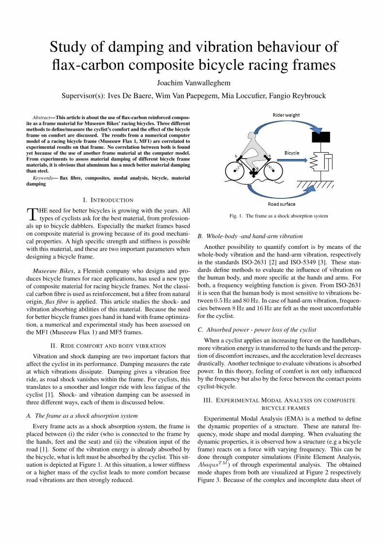
Every frame acts as a shock absorption system, the frame isplaced between (i) the rider (who is connected to the frame bythe hands, feet and the seat) and (ii) the vibration input of theroad [1]. Some of the vibration energy is already absorbed bythe bicycle, what is left must be absorbed by the cyclist. This sit-uation is depicted at Figure 1. At this situation, a lower stiffnessor a higher mass of the cyclist leads to more comfort becauseroad vibrations are then strongly reduced.
Fig. 1. The frame as a shock absorption system
B. Whole-body -and hand-arm vibration
Another possibility to quantify comfort is by means of thewhole-body vibration and the hand-arm vibration, respectivelyin the standards ISO-2631 [2] and ISO-5349 [3]. These stan-dards define methods to evaluate the influence of vibration onthe human body, and more specific at the hands and arms. Forboth, a frequency weighting function is given. From ISO-2631it is seen that the human body is most sensitive to vibrations be-tween 0.5 Hz and 80 Hz. In case of hand-arm vibration, frequen-cies between 8 Hz and 16 Hz are felt as the most uncomfortablefor the cyclist.
C. Absorbed power - power loss of the cyclist
When a cyclist applies an increasing force on the handlebars,more vibration energy is transferred to the hands and the percep-tion of discomfort increases, and the acceleration level decreasesdrastically. Another technique to evaluate vibrations is absorbedpower. In this theory, feeling of comfort is not only influencedby the frequency but also by the force between the contact pointscyclist-bicycle.
III. EXPERIMENTAL MODAL ANALYSIS ON COMPOSITEBICYCLE FRAMES
Experimental Modal Analysis (EMA) is a method to definethe dynamic properties of a structure. These are natural fre-quency, mode shape and modal damping. When evaluating thedynamic properties, it is observed how a structure (e.g a bicycleframe) reacts on a force with varying frequency. This can bedone through computer simulations (Finite Element Analysis,AbaqusTM ) of through experimental analysis. The obtainedmode shapes from both are visualized at Figure 2 respectivelyFigure 3. Because of the complex and incomplete data sheet of

the composite lay-up of the frame, aluminum is applied as mate-rial at the FEA model. This is the reason why there is no matchbetween both.
Fig. 2. MF1: first mode shape from FEA with AbaqusTM
Fig. 3. MF1: first mode shape from EMA
IV. DAMPING PROPERTIES OF ISOTROPIC ANDORTHOTROPIC MATERIALS
Damping is an important parameter of a structure which issubjected to a force. The origin of the force can be due to anunbalance in a rotating structure, a time-varying load, a repeat-ing shock, etc. One parameter which determines the dampingproperty of a structure is the material damping. The type ofmaterial used for the structure will have an influence becauseeach material has other damping properties. Within this scope,the material damping from aluminum, steel, flaxUD and flax-carbon composite has been assessed. Three different kind ofmethods are used, two of them measure response with an ac-celerometer and excitation takes place with an electrodynamicshaker. The shaker can generate a shock or a random vibration,the response of the material due to this excitation is measuredwith an acceleration sensor. These methods are found not tobe adequate to measure damping because of the contact makingelements shaker and accelerometer.
The test setup based on acoustic wave excitation and mea-suring response with a laser vibrometer has more potential to
measure material damping, because this method makes no con-tact with the structure. This is necessary because every elementwhich makes contact with the structure will influence the damp-ing properties of the tested material itself. Until so far, dampingfrom aluminum and steel could be measured adequately. Thedamping profile from both materials is visible at Figure 4. Ma-terial damping of aluminum is twice better than that of steel.Damping properties of flaxUD and flax-carbon reinforced com-
Fig. 4. Acoustic wave excitation: damping profile of steel (blue) and aluminum(yellow)
posite are not yet available because it is not clear how to evaluatethe damping profiles of these materials. In the near future, moreresults will be obtained on this subject.
V. CONCLUSION
Different methods on how to measure and interpret the per-ception of the cyclist on comfort are possible. Two of them arefrequency related, the third one includes a second parameter:contact force between cyclist and bicycle. The latter leads tothe concept absorbed power, this is the power loss of the cy-clist due to cycling on a rough surface. The dynamic behaviourof the MF1 frame has been assessed in a numerical (FEA) andexperimental (EMA) way. The mode shape from EMA is realis-tic but no correlation is found yet with the computer simulationbecause another frame material is used. Finally, the dampingof the bicycle frame material will have an influence on comfortobserved by the cyclist. This makes it necessary to know thedamping properties of frame materials. Measuring damping canbest be done with contactless excitation and response measur-ing. Using such a setup, it could be concluded that aluminumhas twice better damping characteristics compared to steel.
REFERENCES
[1] Craig Calfee and David Kelly, Bicycle frame materials comparison with afocus on carbon fibre construction methods, Technical White Paper, Octo-ber, pp. 1-13, 2004.
[2] International Organization for Standardization ISO 2631-1, Mechanical vi-bration and shock - evaluation of human exposure to whole-body vibration– Part 1: General requirements 1997
[3] International Organization for Standardization ISO 5349-1:2001, Mechan-ical vibration – Measurement and evaluation of human exposure to hand-transmitted vibration – Part 1: General requirements
Contents
Preface iv
Permission for Use of Content v
Survey vi
Contents ix
Samenvatting 1
1 Summary 12
2 Composites 14
2.1 Composites . . . . . . . . . . . . . . . . . . . . . . . . . . . . . . . . . . . . . . . 14
2.2 Flax fibre epoxy as a new material for bicycle frames . . . . . . . . . . . . . . . . 15
2.2.1 Structure and chemical composition . . . . . . . . . . . . . . . . . . . . . 17
2.2.2 Characterization of mechanical properties . . . . . . . . . . . . . . . . . . 18
2.3 How to build a composite bicycle frame . . . . . . . . . . . . . . . . . . . . . . . 18
2.3.1 Composite lay-up . . . . . . . . . . . . . . . . . . . . . . . . . . . . . . . 18
2.3.2 Production process . . . . . . . . . . . . . . . . . . . . . . . . . . . . . . . 19
3 Ride comfort and body vibration 22
3.1 Bicycle frames . . . . . . . . . . . . . . . . . . . . . . . . . . . . . . . . . . . . . 22
3.1.1 The frame as a shock absorption system . . . . . . . . . . . . . . . . . . . 23
3.1.2 Shock absorption versus energy loss . . . . . . . . . . . . . . . . . . . . . 28
3.1.3 Designing a bicycle frame . . . . . . . . . . . . . . . . . . . . . . . . . . . 28
3.2 Body vibration . . . . . . . . . . . . . . . . . . . . . . . . . . . . . . . . . . . . . 29
3.2.1 Whole-body vibration . . . . . . . . . . . . . . . . . . . . . . . . . . . . . 29
3.2.2 Hand-arm vibration . . . . . . . . . . . . . . . . . . . . . . . . . . . . . . 31
3.2.3 Absorbed power . . . . . . . . . . . . . . . . . . . . . . . . . . . . . . . . 32
3.3 Definition of comfort . . . . . . . . . . . . . . . . . . . . . . . . . . . . . . . . . . 33
ix

Contents
4 Vibration analysis on isotropic and orthotropic materials 35
4.1 Introduction . . . . . . . . . . . . . . . . . . . . . . . . . . . . . . . . . . . . . . . 35
4.2 Modal analysis explained in a nutshell . . . . . . . . . . . . . . . . . . . . . . . . 35
4.3 Vibrational analysis on isotropic and orthotropic materials . . . . . . . . . . . . . 37
4.4 Theoretical analysis with AbaqusTM . . . . . . . . . . . . . . . . . . . . . . . . . 37
4.5 Test setup for experimental analysis . . . . . . . . . . . . . . . . . . . . . . . . . 39
4.5.1 The structure under test and its boundary condition setup . . . . . . . . 39
4.5.2 Data acquisition and signal processing . . . . . . . . . . . . . . . . . . . 39
4.5.3 The test setup . . . . . . . . . . . . . . . . . . . . . . . . . . . . . . . . . 41
4.6 Vibration testing on isotropic material . . . . . . . . . . . . . . . . . . . . . . . . 42
4.6.1 Steel beam . . . . . . . . . . . . . . . . . . . . . . . . . . . . . . . . . . . 42
4.6.2 Aluminum plate . . . . . . . . . . . . . . . . . . . . . . . . . . . . . . . . 46
4.6.3 Circular glass plate . . . . . . . . . . . . . . . . . . . . . . . . . . . . . . . 48
4.7 Vibration testing on orthotropic materials . . . . . . . . . . . . . . . . . . . . . . 51
4.7.1 UD-Carbon composite . . . . . . . . . . . . . . . . . . . . . . . . . . . . 51
4.7.2 C-PPS 5 harness satin weave composite . . . . . . . . . . . . . . . . . . . 52
5 Dynamic behaviour of flax/carbon reinforced composite bicycle frames 56
5.1 Introduction . . . . . . . . . . . . . . . . . . . . . . . . . . . . . . . . . . . . . . . 56
5.2 Numerical model of the MF1 frame . . . . . . . . . . . . . . . . . . . . . . . . . . 56
5.2.1 Natural frequencies and mode shapes . . . . . . . . . . . . . . . . . . . . . 57
5.2.2 Influence of tube thickness and frame material . . . . . . . . . . . . . . . 58
5.3 Single Degree Of Freedom: the forced vibration . . . . . . . . . . . . . . . . . . . 58
5.4 Multi Degree Of Freedom: theoretical background . . . . . . . . . . . . . . . . . 61
5.4.1 How to obtain the FRF’s of a MDOF system . . . . . . . . . . . . . . . . 63
5.5 Experimental Modal Analysis . . . . . . . . . . . . . . . . . . . . . . . . . . . . . 64
5.5.1 Excitation of the structure . . . . . . . . . . . . . . . . . . . . . . . . . . 64
5.5.2 Mode Shapes from Quadrature Picking . . . . . . . . . . . . . . . . . . . 65
5.6 Experimental testing: modal properties of the MF1 and MF5 frame . . . . . . . 66
5.6.1 Test setup . . . . . . . . . . . . . . . . . . . . . . . . . . . . . . . . . . . . 66
5.6.2 Mode shape estimation . . . . . . . . . . . . . . . . . . . . . . . . . . . . 68
5.7 Dynamic properties of an assembled bicycle . . . . . . . . . . . . . . . . . . . . . 76
6 Damping properties of isotropic and orthotropic materials 77
6.1 Damping . . . . . . . . . . . . . . . . . . . . . . . . . . . . . . . . . . . . . . . . 77
6.1.1 Importance of damping . . . . . . . . . . . . . . . . . . . . . . . . . . . . 77
6.1.2 Types of damping . . . . . . . . . . . . . . . . . . . . . . . . . . . . . . . 77
6.1.3 Composite damping . . . . . . . . . . . . . . . . . . . . . . . . . . . . . . 78
6.1.4 Damping models . . . . . . . . . . . . . . . . . . . . . . . . . . . . . . . . 78
6.2 Measuring damping . . . . . . . . . . . . . . . . . . . . . . . . . . . . . . . . . . 79
x

Contents
6.2.1 Damping factor from the time domain . . . . . . . . . . . . . . . . . . . . 79
6.2.2 Damping factor from the frequency domain . . . . . . . . . . . . . . . . . 82
6.3 Damping properties from shaker excitation: method 1 . . . . . . . . . . . . . . . 82
6.3.1 Test setup . . . . . . . . . . . . . . . . . . . . . . . . . . . . . . . . . . . . 82
6.3.2 Results . . . . . . . . . . . . . . . . . . . . . . . . . . . . . . . . . . . . . 85
6.4 Damping properties from shaker excitation: method 2 . . . . . . . . . . . . . . . 91
6.4.1 Test setup . . . . . . . . . . . . . . . . . . . . . . . . . . . . . . . . . . . . 91
6.4.2 Results . . . . . . . . . . . . . . . . . . . . . . . . . . . . . . . . . . . . . 93
6.5 Damping properties from acoustic wave excitation . . . . . . . . . . . . . . . . . 95
6.5.1 Test setup . . . . . . . . . . . . . . . . . . . . . . . . . . . . . . . . . . . . 95
6.5.2 Results . . . . . . . . . . . . . . . . . . . . . . . . . . . . . . . . . . . . . 96
6.6 Conclusion . . . . . . . . . . . . . . . . . . . . . . . . . . . . . . . . . . . . . . . 100
7 Conclusion 101
7.1 How to quantify the cyclist’s comfort . . . . . . . . . . . . . . . . . . . . . . . . . 101
7.2 Frame optimization . . . . . . . . . . . . . . . . . . . . . . . . . . . . . . . . . . . 101
7.3 Test setup to measure damping . . . . . . . . . . . . . . . . . . . . . . . . . . . . 102
7.4 Further research . . . . . . . . . . . . . . . . . . . . . . . . . . . . . . . . . . . . 102
A Data sheets and drawings 104
A.1 Accelerometers . . . . . . . . . . . . . . . . . . . . . . . . . . . . . . . . . . . . . 104
A.2 Force sensor . . . . . . . . . . . . . . . . . . . . . . . . . . . . . . . . . . . . . . 104
A.3 Data sheet shaker and Power Amplifier . . . . . . . . . . . . . . . . . . . . . . . 104
A.4 2D Drawings MF1 and MF5 frame . . . . . . . . . . . . . . . . . . . . . . . . . . 104
A.5 Parts used for testing . . . . . . . . . . . . . . . . . . . . . . . . . . . . . . . . . 104
Bibliography 120
xi
Samenvatting
Inleiding
Fietsen, en dan vooral op professioneel niveau, gaat op alle gebied gepaard met
(hoog)technologische vooruitgang. Zo is tijdens een tijdrit de positie van de renner op
de fiets van groot belang, aldus wordt er gezocht hoe de luchtweerstand kan verminderd worden.
Hierbij worden testen gedaan in windtunnels om de houding van de renner aan te passen maar
ook om eventueel aanpassingen te doen aan het fietsframe. Ook de ontwikkeling naar betere
onderdelen zoals versnellingen, remmen, wielen, banden,... staat niet stil. Al deze aspecten
zorgen ervoor dat de fietser betere prestaties kan leveren.
Echter, de belangrijkste component aan de fiets is nog steeds het frame zelf. Hoezeer men ook
alle andere gebieden van fietsoptimalisatie beheerst, zonder een frame van topkwaliteit worden
ook geen topprestaties geleverd. De wensen van de renner zijn eenvoudig: hij wil een frame
dat licht, stijf, duurzaam, sterk, mooi, niet corrodeert en dan ook nog eens comfortabel is. De
ontwikkelaar van het frame staat dus voor een heuse opdracht, want een frame dat aan al deze
aspecten tegelijk moet voldoen is haast ondenkbaar. Zo zijn bijvoorbeeld stijfheid en comfort
twee tegenpolen van elkaar, aldus moet men een compromis zoeken tussen beide. Afhankelijk
van het gebruikte materiaal voor het frame kan men aan de een of ander wens beter voldoen.
Het doel van dit afstudeerwerk is om het dynamamisch aspect te onderzoeken in de optimalisatie
naar het fietsframe. Dit wil zeggen dat wordt onderzocht hoe het frame reageert als het
onderhevig is aan krachten ten gevolge van trillingen tijdens het fietsen op de weg. Het gedrag
van het frame is van groot belang voor het comfortgevoel van de fietser. Want hoe beter de
trillingen van de weg kunnen geabsorbeerd worden door het fietskader, hoe beter de renner zal
preseteren. Trillingen die niet worden opgevangen door de fiets (het frame) worden geabsorbeerd
door de renner en dit leidt tot vermoeiing van de spieren met als gevolg verminderde prestaties.
Onderzoek naar het dynamisch gedrag van materiaal leidt uiteindelijk tot een beter fietsframe,
waardoor men weer een stap dichter is bij het ideale frame.
Omschrijving van het onderzoek
Deze thesis verloopt in samenwerking met Museeuw Bikes, dit is een Vlaams bedrijf dat instaat
voor het ontwerp en productie van fietsframes voor race toepassingen. De frames van Museeuw
1
Samenvatting
Bikes zijn gemaakt uit vezelversterkte kunststoffen, het zogenaamde composiet frame. Veelal
zijn composiet frames versterkt met koolstofvezel, dit zijn de gekende carbon composiet frames.
Museeuw Bikes heeft echter geopteerd om niet 100 % koolstofvezel te gebruiken maar een
combinatie van koolstofvezel en vlasvezel. Die laatste is een vezel van natuurlijke oorsprong
en zijn toepassing op de markt van de fietskaders is nieuw. Van hen uit kwam de opdracht om
dit materiaal te onderzoeken, zowel op statisch [1] als dynamisch niveau, de resultaten hieruit
kunnen uiteindelijk leiden tot optimalisatie van het frame naar gewicht, stijfheid en comfort.
In dit afstudeerwerk wordt voor een goed begrip eerst ingegaan op de vezelversterkte
kunststoffen, het composiet. Wat zijn hiervan de voornaamste eigenschappen, kenmerken en
welke zijn hierbij belangrijk voor het ontwerp van een fietskader. Verder wordt verklaard wat
comfort is en hoe men dit kan kwantificeren. Er zijn reeds een aantal studies gebeurd die
onderzoek hebben gedaan naar het effect van trillingen tijdens het fietsen op het menselijke
lichaam. Zo kan een betere schokabsorptie leiden tot meer comfort, maar resulteert het ook
niet tot absorptie van het geleverd vermogen in het frame? Uit eerder onderzoek blijkt dat
het energieverlies door het dempingssysteem (bij een mountainbike) meer dan gecompenseerd
wordt door winst die de renner haalt uit verminderde blootstelling aan trillingen [2, 3].
Als eerste stap in het onderzoek wordt een trillingsanalye uitgevored op structuren waarvan
alle eigenschappen gekend zijn. Hierbij wordt bepaald hoe een structuur zich gedraagt als
deze onderhevig is aan een uitwendige trilling. Reeds in deze fase van het onderzoek wordt
belangrijke kennis opgedaan over het uitvoeren van trillingstesten, zowel in het labo als met
computersimulaties. Vervolgens wordt het dynamisch gedrag bepaald van het MF1 en MF5
frame, dit zijn twee modellen uit het gamma van Museeuw Bikes. Zoals eerder gezegd zijn
dat frames op basis van vlas-carbon vezelversterkte kunststoffen, ofwel vlas-carbon composiet.
Experimentele Modale Analyse (EMA) is hierbij een methode om het dynamisch gedrag van een
structuur te bepalen. Van het MF1 frame wordt ook een numeriek computermodel gemaakt,
vertrekkende van dit model kunnen computersimulaties gedaan worden die in feite hetzelfde
resultaat zouden moeten weergeven als hetgeen is verkregen door middel van EMA. De resultaten
hiervan kunnen vervolgens gecorreleerd worden met de resultaten die volgen uit EMA. Zodoende
kan men het frame numeriek gaan optimaliseren zonder dat verder experimenten vereist zijn.
Als laatste worden de dempingseigenschappen van verschillende framematerialen bepaald. De
twee courante materialen aluminium en staal worden vergeleken met de composieten op basis
van carbon, vlas en vlas-carbon. Aan de hand van deze testen wordt dus bepaald welk materiaal
de beste materiaaldemping heeft.
Composieten
Algemeen beschouwd is een composiet een niet-homogeen materiaal dat bestaat uit minstens
twee verschillende materialen (de matrix en de vezel). Een typisch voorbeeld is versterkt beton,
de staalconstructie is de vezel terwijl het beton de matrix is. Het type composiet dat gebruikt
2
Samenvatting
wordt als materiaal voor fietskaders is een vezelversterkte kunststof. Dit composiet is van
dezelfde soort als hetgeen gebruikt wordt voor toepassingen in de lucht- en ruimtevaart. Een
vezelversterkte kunststof bestaat uit een kunststof (de matrix) en een vezel. De vezel kan van
natuurlijke (vlas, bamboe,...) of synthetische oorsprong zijn (koolstof, glas,...). De vezel geeft
het materiaal sterkte en stijfheid, terwijl de kunststof zich rond de vezels bevindt en moet
zorgen voor een goede overdracht van kracht tussen de vezels onderling. De kunststof zorgt ook
voor afscherming van de vezels aan de buitenwereld [4]. Een voordeel van dit materiaal is de
hoge specifieke sterkte en stijfheid, dit wil zeggen dat het materiaal zeer sterk en stijf is terwijl
het toch zeer weinig weegt. Hierbij is alvast aan drie wensen voldaan: een lichtgewicht frame
dat toch sterk en stijf is. Het materiaal leent zich ook tot complexe vormgeving, wat ook van
toepassing is in het geval van een fietskader. De lage taaiheid van composieten kan echter leiden
tot een brosse breuk bij beschadiging van het frame wat onverwachte effecten met zich mee kan
brengen.
De keuze van Museeuw Bikes om vlas als versterkingsvezel te gebruiken is niet zomaar. Vlas
heeft de beste mechanische eigenschappen [5] van alle natuurlijke vezels en het zou ook betere
trillingsdempende eigenschappen hebben in vergelijking met de carbonvezel. Dit laatste kan dan
weer ten goede komen voor het comfortgevoel van de fietser.
Een fietsframe is veelal een serieproduct en daarom wordt gebruikt gemaakt van een mal voor
de productie ervan. In eerste instantie is de vezel geımpregneerd in het kunststof, dit vormt
een laag met een dikte van typisch 0.2 mm. Dit heet men een Pre-Preg. Deze lagen worden
vervolgens met de gewenste richting en aantal lagen in de mal geplaatst. Vervolgens is het
product onderhevig aan een temperatuur- en drukcyclus. Dit zorgt ervoor dat de structuur vast
wordt en de gewenste eigenschappen krijgt. In het labo wordt dit proces verwezenlijkt met een
autoklaaf.
Comfort en lichaamstrillingen
Trillingen en schokdemping zijn twee factoren waardoor de fietser beınvloed wordt. Echter, dit
zijn twee begrippen die moeilijk te begrijpen zijn in de materiaalkunde. Er zijn bij het proces
van schokdemping zodanig veel parameters die dit kunnen beınvloeden dat het moeilijk is om te
voorspellen hoe een structuur zal reageren als die onderhevig is aan externe krachten/trillingen
[6].
Een eerste model modelleert de fiets als een stijfheid k en een demper c die zich bevinden tussen
het wegdek en de renner. Grafisch kan dit voorgesteld worden als op figuur 1.
3

Samenvatting
Figuur 1: Voorstelling van frame als veer-demper systeem tussen wegdek en fietser
Het frame is geplaatst tussen (i) de fietser (die is verbonden met het frame via de handen, het
zitvlak en de voeten) en (ii) de trillingsinput van het wegdek. De trillingsinput is afkomstig
van oneffenheden op het wegdek. Deze oneffenheden worden doorgegeven via de band, de velg
en de spaken tot de as van het wiel. Ter hoogte van de as worden de trillingen onverminderd
doorgegeven naar het frame. Nu is het frame bepalend voor het doorgeven van trillingen naar de
fietser. De schematische voorstelling van wegdek-frame-renner (figuur 1) kan nu gebruikt worden
als input voor passieve trillingscontrole. De wegtrilling wordt voorgesteld als y(t) = y0ejωt; het
frame als een stijfheid k en een demper c; de trilling ter hoogte van de fietser met massa m is
dan q(t) zoals te zien op figuur 2.
Figuur 2: Passieve trillingscontrole: fiets (k en c)+ fietser m [7]
Uit de bewegingsvergelijking van dit systeem kan de verhouding van de amplitude van q(t) en
4

Samenvatting
y(t) bepaald worden. Na uitwerken volgt:
TR =∣∣∣∣qy∣∣∣∣ =
q0
y0=
√1 +
(2ζ ω
ωn
)√(
1−(ωωn
)2)2
+(
2ζ ωωn
)2
Waarbij ωn =√
km de eigenfrequentie van het systeem is en ζ = c
2mωnde dempingsfactor. Een
grafische voorstelling van bovenstaande vergelijking geeft een duidelijker beeld, te zien op figuur
3.
Figuur 3: Overdraagbaarheid wegdek - fietser
Effectieve demping (TR < 1) vindt plaats voor ωωn
>√
2. Dit wil zeggen dat de
trillingsamplitude van het wegdek verminderd wordt doorgegeven naar de fietser. Voor ωωn
> 3
wordt minder dan 10 % van de wegoneffenheid doorgegeven naar de fietser. Demping speelt
enkel een rol in de nabijheid van de resonantiepiek ωωn
= 1. Verder moet voor een lage TR
de eigenfrequentie van het systeem zo laag mogelijk gehouden worden, dit kan door door de
stijfheid van het frame te verlagen of de massa ervan te verhogen. Een minder stijf frame
leidt in dat opzicht tot meer comfort. Het is wel van groot belang om te realiseren dat de
frequentie van de wegtrilling ω niet constant is en in realiteit het fietsframe complexer is dan
deze vereenvoudigde voorstelling.
Een ander aspect bij het bespreken van comfort is de perceptie van het menselijk lichaam op
externe trillingen. De ISO-2631 norm [8] is hiervoor ontwikkeld. Hieruit blijkt dat vooral in
het frequentiegebied van 0.5 Hz tot 80 Hz het menselijk lichaam gevoelig is voor trillingen (zie
figuur 4). Aangezien de fietser ook onderhevig is aan trillingen ter hoogte van de armen moet
ook hier de trilling geevalueerd worden. Hiervoor is de norm ISO 5349-1 [9] beschikbaar, deze
stelt dat in het frequentiegebied van 8 Hz tot 16 Hz de handen en armen het meest gevoelig zijn
aan trillingen.
5

Samenvatting
Figuur 4: Frequentieweging in geval van een zittend persoon (Wk: z-richting, Wd: x- en y-richting en
Wt: misselijkheid) [8]
Niet enkel trillingen zijn van belang, maar ook het geabsorbeerd vermogen door de fietser kan
bepaald worden. Hier is niet enkel de frequentie van belang, maar ook de kracht tussen de
contactpunten fietser/fiets. Een combinatie van frequentie en verplaatsing leidt tot een bepaald
vermogenverlies van de fietser [10]. De verplaatsing zal afhangen van hoe stevig de fietser zich
begeeft op de fiets. Indien bijvoorbeeld het stuur steviger wordt vast gehouden leidt dit tot meer
overdracht van trillingen naar het lichaam dan indien het stuur weinig wordt vast gegrepen.
Echter, als de kracht op deze contactpunten wijzigt, verandert ook het totale dynamisch gedrag
(van fiets en fietser) aangezien er meer koppeling is tussen beide [11].
Trillingsanalyse van isotrope en orthotrope materialen
Het uitvoeren van een trillingsanalyse is eigenlijk het bepalen van de dynamische eigenschappen
van structuren. Drie parameters kunnen hierbij bepaald worden: eigenfrequentie, modale
demping en modevormen. Typisch aan een structuur (een voorwerp) is dat, als deze onderhevig
is aan een kracht met een varierende frequentie, ze afhankelijk van de frequentie van de kracht
hierop verschillend zal reageren. Voor bepaalde frequenties zal de structuur veel heviger gaan
trillen (en dus vervormen) en hierbij neemt de structuur een bepaalde vevorming aan. De eerste
parameter is dan de eigenfrequentie, de bijhorende vervorming is de modevorm. Ten derde
bezit elke structuur demping, deze wordt gekarakteriseerd door de modale dempingsfactor. Deze
parameter is afhankelijk van de frequentie.
In eerste instantie worden trillingstesten uitgevoerd op eenvoudige structuren waarvan alle
parameters gekend zijn om zo de gemeten resultaten te kunnen vergelijken met resultaten
6
Samenvatting
afkomstig van computersimulaties. In een later stadium kunnen dan de fietsframes op een
analoge manier getest worden. Met deze trillingsanalyse worden enkel de eigenfrequenties
bepaald van verschillende structuren, zowel isotroop als orthotroop. Een isotroop materiaal
heeft als kenmerk dat al zijn eigenschappen identiek zijn in alle richtingen, zo is bijvoorbeeld
de Young’s modulus onafhankelijk van de richting. Daarentegen zijn de eigenschappen van
een orthotroop materiaal verschillend voor de drie richtingen (x,y en z). Bij een orthotroop
materiaal (een composiet) kunnen drie onderling loodrechte vlakken gedefineerd worden waarin
de eigenschappen dezelfde zijn.
De geteste isotrope materialen zijn een plaat aluminium, een stalen ligger en een ronde
glasplaat. Als orthotroop materiaal wordt er gekozen voor twee soorten koolstofvezel versterkte
kunststoffen. Van dergelijke structuren kunnen via computersimulatie de eigenfrequenties
bepaald worden. Als computerprogramma wordt gebruik gemaakt van AbaqusTM , dit is een
eindige elementenpakket dat het gedrag van structuren kan bepalen die onderhevig zijn aan
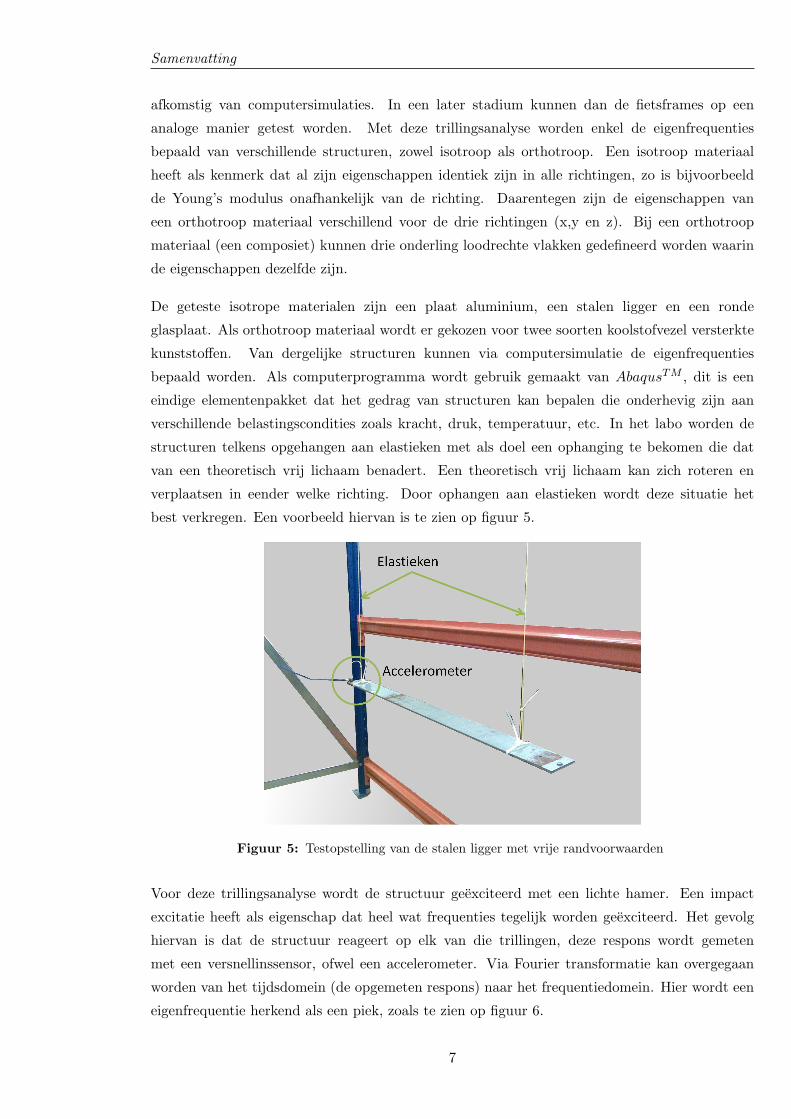
verschillende belastingscondities zoals kracht, druk, temperatuur, etc. In het labo worden de
structuren telkens opgehangen aan elastieken met als doel een ophanging te bekomen die dat
van een theoretisch vrij lichaam benadert. Een theoretisch vrij lichaam kan zich roteren en
verplaatsen in eender welke richting. Door ophangen aan elastieken wordt deze situatie het
best verkregen. Een voorbeeld hiervan is te zien op figuur 5.
Figuur 5: Testopstelling van de stalen ligger met vrije randvoorwaarden
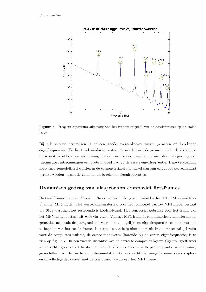
Voor deze trillingsanalyse wordt de structuur geexciteerd met een lichte hamer. Een impact
excitatie heeft als eigenschap dat heel wat frequenties tegelijk worden geexciteerd. Het gevolg
hiervan is dat de structuur reageert op elk van die trillingen, deze respons wordt gemeten
met een versnellinssensor, ofwel een accelerometer. Via Fourier transformatie kan overgegaan
worden van het tijdsdomein (de opgemeten respons) naar het frequentiedomein. Hier wordt een
eigenfrequentie herkend als een piek, zoals te zien op figuur 6.
7
Samenvatting
Figuur 6: Frequentiespectrum afkomstig van het responsiesignaal van de accelerometer op de stalen
ligger
Bij alle geteste structuren is er een goede overeenkomst tussen gemeten en berekende
eigenfrequenties. Er dient wel aandacht besteed te worden aan de geometrie van de structuur.
Zo is vastgesteld dat de vervorming die aanwezig was op een composiet plaat ten gevolge van
thermische restspanningen een grote invloed had op de eerste eigenfrequentie. Deze vervorming
moet mee gemodelleerd worden in de computersimulatie, enkel dan kan een goede overeenkomst
bereikt worden tussen de gemeten en berekende eigenfrequenties.
Dynamisch gedrag van vlas/carbon composiet fietsframes
De twee frames die door Museeuw Bikes ter beschikking zijn gesteld is het MF1 (Museeuw Flax
1) en het MF5 model. Het versterkingsmateriaal voor het composiet van het MF1 model bestaat
uit 50 % vlasvezel, het resterende is koolstofvezel. Het composiet gebruikt voor het frame van
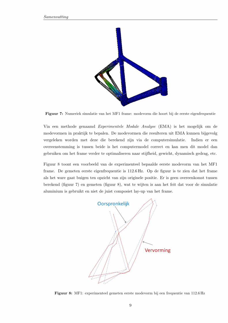
het MF5 model bestaat uit 80 % vlasvezel. Van het MF1 frame is een numeriek computer model
gemaakt, net zoals de paragraaf hiervoor is het mogelijk om eigenfrequenties en modevormen
te bepalen van het totale frame. In eerste instantie is aluminium als frame materiaal gebruikt
voor de computersimulatie, de eerste modevorm (horende bij de eerste eigenfrequentie) is te
zien op figuur 7. In een tweede instantie kan de correcte composiet lay-up (lay-up: geeft weer
welke richting de vezels hebben en wat de dikte is op een welbepaalde plaats in het frame)
gemodelleerd worden in de computersimulatie. Tot nu was dit niet mogelijk wegens de complexe
en onvolledige data sheet met de composiet lay-up van het MF1 frame.
8
Samenvatting
Figuur 7: Numeriek simulatie van het MF1 frame: modevorm die hoort bij de eerste eigenfrequentie
Via een methode genaamd Experimentele Modale Analyse (EMA) is het mogelijk om de
modevormen in praktijk te bepalen. De modevormen die resulteren uit EMA kunnen bijgevolg
vergeleken worden met deze die berekend zijn via de computersimulatie. Indien er een
overeenstemming is tussen beide is het computermodel correct en kan men dit model dan
gebruiken om het frame verder te optimaliseren naar stijfheid, gewicht, dynamisch gedrag, etc.
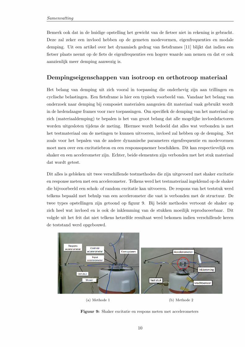
Figuur 8 toont een voorbeeld van de experimenteel bepaalde eerste modevorm van het MF1
frame. De gemeten eerste eigenfrequentie is 112.6 Hz. Op de figuur is te zien dat het frame
als het ware gaat buigen ten opzicht van zijn originele positie. Er is geen overeenkomst tussen
berekend (figuur 7) en gemeten (figuur 8), wat te wijten is aan het feit dat voor de simulatie
aluminium is gebruikt en niet de juist composiet lay-up van het frame.
Figuur 8: MF1: experimenteel gemeten eerste modevorm bij een frequentie van 112.6 Hz
9
Samenvatting
Bemerk ook dat in de huidige opstelling het gewicht van de fietser niet in rekening is gebracht.
Deze zal zeker een invloed hebben op de gemeten modevormen, eigenfrequenties en modale
demping. Uit een artikel over het dynamisch gedrag van fietsframes [11] blijkt dat indien een
fietser plaats neemt op de fiets de eigenfrequenties een hogere waarde aan nemen en dat er ook
aanzienlijk meer demping aanwezig is.
Dempingseigenschappen van isotroop en orthotroop materiaal
Het belang van demping uit zich vooral in toepassing die onderhevig zijn aan trillingen en
cyclische belastingen. Een fietsframe is hier een typisch voorbeeld van. Vandaar het belang van
onderzoek naar demping bij composiet materialen aangezien dit materiaal vaak gebruikt wordt
in de hedendaagse frames voor race toepassingen. Om specifiek de demping van het materiaal op
zich (materiaaldemping) te bepalen is het van groot belang dat alle mogelijke invloedsfactoren
worden uitgesloten tijdens de meting. Hiermee wordt bedoeld dat alles wat verbonden is met
het testmateriaal om de metingen te kunnen uitvoeren, invloed zal hebben op de demping. Net
zoals voor het bepalen van de andere dynamische parameters eigenfrequentie en modevormen
moet men over een excitatiebron en een responsopnemer beschikken. Dit kan respectievelijk een
shaker en een accelerometer zijn. Echter, beide elementen zijn verbonden met het stuk materiaal
dat wordt getest.
Dit alles is gebleken uit twee verschillende testmethodes die zijn uitgevoerd met shaker excitatie
en response meten met een accelerometer. Telkens werd het testmateriaal ingeklemd op de shaker
die bijvoorbeeld een schok- of random excitatie kan uitvoeren. De respons van het teststuk werd
telkens bepaald met behulp van een accelerometer die vast is verbonden met de structuur. De
twee types opstellingen zijn getoond op figuur 9. Bij beide methodes vertoont de shaker op
zich heel wat invloed en is ook de inklemming van de stukken moeilijk reproduceerbaar. Dit
volgde uit het feit dat niet telkens hetzelfde resultaat werd bekomen indien verschillende keren
de teststand werd opgebouwd.
(a) Methode 1 (b) Methode 2
Figuur 9: Shaker excitatie en respons meten met accelerometers
10
Contents
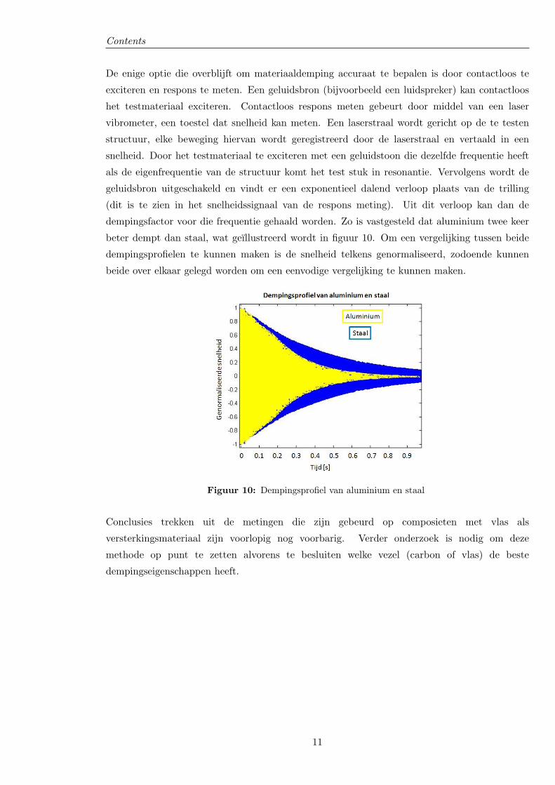
De enige optie die overblijft om materiaaldemping accuraat te bepalen is door contactloos te
exciteren en respons te meten. Een geluidsbron (bijvoorbeeld een luidspreker) kan contactloos
het testmateriaal exciteren. Contactloos respons meten gebeurt door middel van een laser
vibrometer, een toestel dat snelheid kan meten. Een laserstraal wordt gericht op de te testen
structuur, elke beweging hiervan wordt geregistreerd door de laserstraal en vertaald in een
snelheid. Door het testmateriaal te exciteren met een geluidstoon die dezelfde frequentie heeft
als de eigenfrequentie van de structuur komt het test stuk in resonantie. Vervolgens wordt de
geluidsbron uitgeschakeld en vindt er een exponentieel dalend verloop plaats van de trilling
(dit is te zien in het snelheidssignaal van de respons meting). Uit dit verloop kan dan de
dempingsfactor voor die frequentie gehaald worden. Zo is vastgesteld dat aluminium twee keer
beter dempt dan staal, wat geıllustreerd wordt in figuur 10. Om een vergelijking tussen beide
dempingsprofielen te kunnen maken is de snelheid telkens genormaliseerd, zodoende kunnen
beide over elkaar gelegd worden om een eenvodige vergelijking te kunnen maken.
Figuur 10: Dempingsprofiel van aluminium en staal
Conclusies trekken uit de metingen die zijn gebeurd op composieten met vlas als
versterkingsmateriaal zijn voorlopig nog voorbarig. Verder onderzoek is nodig om deze
methode op punt te zetten alvorens te besluiten welke vezel (carbon of vlas) de beste
dempingseigenschappen heeft.
11
Chapter 1
Summary
Riding a bicycle, and mainly at professional level, goes hand in hand with the improvement of
state of the art technology. For instance, during a time trial the position of the cyclist is of
big importance. For this reason, it is important how air resistance can be reduced. Tests have
already been done in wind tunnels to search for the best position on the bicycle, eventually also
small adaptations at the frame are possible. This is only one aspect, also research for better
gears, brakes, tyres, wheels, etc. makes progress. Al these aspects cause the cyclist to achieve
better results.
However, the main component on a bicycle is still the frame itself. Even if all the other aspects of
the bicycle are of top quality, no top performance will be achieved without a frame of the highest
quality. The cyclist wants his bicycle to be light, stiff, durable, strong, nice looking, weather
resistant and it must also be comfortable. The developer of bicycle faces a great challange,
because designing a frame which meets all these requirements is barely impossible. For example,
stiffness and comfort are eachothers opposite, though a compromise between both must be found.
Depending on the used material for the frame, one or other aspect can be fulfilled better.
The goal of this master thesis is to investigate the dynamic behaviour of the bicycle frame
itself, which is only one single piece of the puzzle to frame optimization. Dynamic behaviour
means how the frame reacts when its submitted to forces due to vibrations coming from the
irregularities on the road surface. The behaviour of the frame is of big importance for the
perception on comfort of the rider. Because, the better vibrations coming from the road are
absorbed by the frame, the better the rider will perform. Vibrations which are not absorbed by
the bicycle (frame) must be absorbed by the rider and this causes fatigue of the muscles and
thus diminished performance. Research to the aspect of the dynamic behaviour eventually leads
to a better frame, so one gets one step closer to the ideal bicycle frame.
12
Chapter 1. Summary
Description of the study
This master thesis is in close collaboration with Museeuw Bikes, this a Flemish company which
stands in for design and production of bicycle frames for race applications. The frames from
Museeuw Bikes are made of fibre reinforced polymers, the so called composite frame. Mainly
composite frames are reinforced with carbon fibre, these are the well known carbon composite
frames. However, Museeuw Bikes has chosen not to use 100 % carbon fibre, but a combination of
carbon fibre and flax fibre. The latter is a fibre from natural origin en its use is new in the bicycle
frame industry. Museeuw Bikes gave us the task to investigate this material, on both static [1]
and dynamic level. The results coming from this research eventually can lead to optimization
of the frame on weight, stiffness and comfort.
For a good understanding, first more explanation is given about fibre reinforced polymers. What
are the main properties, characteristics and which of them are important in frame bicycle design.
Further, based on literature study a definition of comfort is given. Also, more is said about how
comfort can be quantified. Already some studies have been assessed which describe the effect
of vibrations on the human body during bicycling. Shock absorption leads definitely to more
comfort, but does it also lead to more power loss of the rider due to deformation of the frame?
A conclusion that counts for the different studies [2, 3] is that the magnitude of any energy
dissipation by a suspension system must by very small, if any, and thus probably negligible
compared with the advantages they provide.
As a first step in the experimental research, vibration analysis on structures from which all the
properties are known has been assessed. Hereby is determined how a structure behaves when
this is subjected to a external vibration. Already at this stage of the research some important
knowledge on doing vibration analysis (in the lab and with computer simulations) is acquired.
After this is finished, the dynamic behaviour of the MF1 and MF5 frame is determined. These
are two frame models which are made of the flax-carbon composite material. Experimental
Modal Analysis (EMA) is a useful tool to get in an experimental way the dynamic properties
form a structure. Also a numerical computer model has been built, starting from this model
it is possible do computer simulations which give the same results as those received in the lab
(by means of EMA). The results from the computer simulation are then correlated with the
results from experiments (EMA). In this way it is possible to optimize a frame in a numerical
way without the need for time-consuming experiments. As a last part in this master thesis,
the damping properties of different frame materials are assessed. The two common materials
aluminum and steel are compared with the composites based on carbon, flax and flax-carbon.
13
Chapter 2
Composites
2.1 Composites
Generally, a composite material can be defined as a non homogeneous material which consists
of at least two individual materials. These components are clearly noticeable, and thus between
two components a clear boundary line exists. There are two categories of constituent materials:
matrix and reinforcement. The matrix material surrounds and supports the reinforcement
materials by maintaining their relative positions. The reinforcements impart their mechanical
and physical properties to enhance the matrix properties. Examples of composites are reinforced
concrete, car tyres, multiplex, etc. High-grade composites are based on high-grade fibres inserted
into a high-grade polymer, a metal or another material. This fibre reinforced material is used as
construction material due to its mechanical properties. The material has very good mechanical
properties (strength and stiffness) in the direction of the fibre, combined with a low mass density.
The stiffness of a component means how much it deflects under a given load. The strength of
a material is its resistance to failure by permanent deformation. The mechanical properties
depend on the direction of the fibre, this gives the material an anisotropic character. This is in
contrast with isotropic materials such as steel and aluminum, there the material properties are
the same in every direction.
For both the matrix and the reinforcement different materials can be used. The most common
reinforcements are glass fibres, organic fibres, carbon fibres, metal fibres and ceramic fibres. For
the matrix material, often polymers (thermosets and thermoplastics), metals, carbon, ceramic
and glass are used [4]. The first category (i) is that of fibre reinforced polymers (FRP). The
composite exists of a polymer matrix (the resin) reinforced with glass-, carbon- or organic fibres.
A polymer is a large molecule which consists of repeating structural units. The polymer is usually
a thermoset or a thermoplast. In case of a thermoset (e.g. epoxy) the polymer is cross-linked, a
3-D network of bonds is formed. This is in contrast with a thermoplast, where no cross-linking
is present. As a consequence, a thermoset is stronger and is better suited for high temperature
applications. The second category (ii), the metal matrix composite (MMC), is formed when a
metal matrix is used, the other material may be a different metal or another material, such as
14
Chapter 2. Composites
a ceramic or organic compound. At last (iii) the carbon-carbon composite (CCC) is formed by
inserting a carbon fibre into a graphite matrix.
The FRP are mostly used for mechanical constructions because of some interesting advantages
such as (i) the strength and stiffness of the fibres together with the low density of the resin, and
(ii) the resin which is corrosion resistant and it makes producing complex shapes possible [12].
Other advantages of composites are the high stiffness to weight ratio (specific stiffness), which
makes them ideal for lightweight structures, such as bicycle frames. More energy absorption
is possible compared to applications based on isotropic materials (steel, aluminum, copper,
etc.) and it is also wear-resistant [12]. But composites also have their drawbacks, for instance
the production process is mostly manual, if any serial production is desired, a costly mold is
necessary. Also the high cost of the fibres and the matrix makes that composites are mostly
used for specific applications. The air- and space travel is a known sector, but also sport articles
such as tennis rackets, bicycle frames, etc. make use of the benefits of composites.
2.2 Flax fibre epoxy as a new material for bicycle frames
The joy of riding a bicycle is enhanced with the invention of new materials, the development of
new technologies and design procedures that improve comfort and durability. Steel, titanium
and aluminum are materials still used in the industry but carbon fibre reinforced polymer is
becoming the most popular - certainly for race bicycles - material for frames and for almost all
bike components [11]. In case of bicycle frames, epoxy is used as matrix material (resin). Carbon
fibre is used as reinforcement fibre because of its high specific stiffness and specific strength.
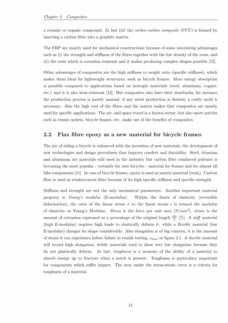
Stiffness and strength are not the only mechanical parameters. Another important material
property is Young’s modulus (E-modulus). Within the limits of elasticity (reversible
deformation), the ratio of the linear stress σ to the linear strain ε is termed the modulus
of elasticity or Young’s Modulus. Stress is the force per unit area [N/mm2], strain is the
amount of extension expressed as a percentage of the original length ∆LL [%]. A stiff material
(high E-modulus) requires high loads to elastically deform it, while a flexible material (low
E-modulus) changes its shape considerably. Also elongation is of big concern, it is the amount
of strain it can experience before failure in tensile testing, εmax at figure 2.1. A ductile material
will record high elongation, brittle materials tend to show very low elongation because they
do not plastically deform. At last, toughness is a measure of the ability of a material to
absorb energy up to fracture when a notch is present. Toughness is particulary important
for components which suffer impact. The area under the stress-strain curve is a criteria for
toughness of a material.
15
Chapter 2. Composites
Figure 2.1: Stress-Strain diagram
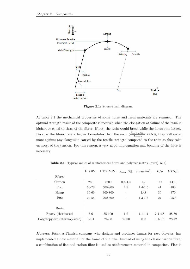
At table 2.1 the mechanical properties of some fibres and resin materials are summed. The
optimal strength result of the composite is received when the elongation at failure of the resin is
higher, or equal to these of the fibres. If not, the resin would break while the fibres stay intact.
Because the fibres have a higher E-modulus than the resin (Ecarbonfibre
Eepoxy≈ 50), they will resist
more against any elongation caused by the tensile strength compared to the resin so they take
up most of the tension. For this reason, a very good impregnation and bonding of the fibre is
necessary.
Table 2.1: Typical values of reinforcement fibres and polymer matrix (resin) [5, 4]
E [GPa] UTS [MPa] εmax [%] ρ [kg/dm3] E/ρ UTS/ρ
Fibres
Carbon 250 2500 0.4-1.4 1.7 147 1470
Flax 50-70 500-900 1.5 1.4-1.5 41 480
Hemp 30-60 300-800 - 1.48 30 370
Jute 20-55 200-500 - 1.3-1.5 27 250
Resin
Epoxy (thermoset) 3-6 35-100 1-6 1.1-1.4 2.4-4.8 28-80
Polypropyleen (thermoplastic) 1-1.4 25-38 >300 0.9 1.1-1.6 28-42
Museeuw Bikes, a Flemish company who designs and produces frames for race bicycles, has
implemented a new material for the frame of the bike. Instead of using the classic carbon fibre,
a combination of flax and carbon fibre is used as reinforcement material in composites. Flax is
16
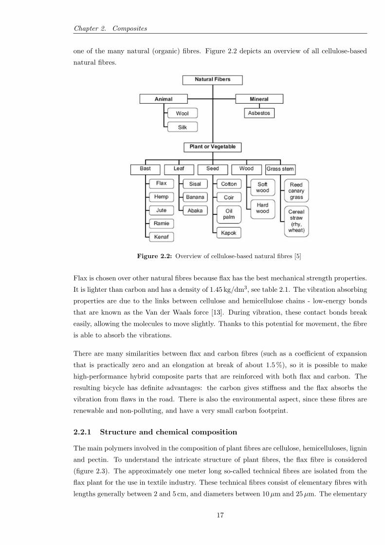
Chapter 2. Composites
one of the many natural (organic) fibres. Figure 2.2 depicts an overview of all cellulose-based
natural fibres.
Figure 2.2: Overview of cellulose-based natural fibres [5]
Flax is chosen over other natural fibres because flax has the best mechanical strength properties.
It is lighter than carbon and has a density of 1.45 kg/dm3, see table 2.1. The vibration absorbing
properties are due to the links between cellulose and hemicellulose chains - low-energy bonds
that are known as the Van der Waals force [13]. During vibration, these contact bonds break
easily, allowing the molecules to move slightly. Thanks to this potential for movement, the fibre
is able to absorb the vibrations.
There are many similarities between flax and carbon fibres (such as a coefficient of expansion
that is practically zero and an elongation at break of about 1.5 %), so it is possible to make
high-performance hybrid composite parts that are reinforced with both flax and carbon. The
resulting bicycle has definite advantages: the carbon gives stiffness and the flax absorbs the
vibration from flaws in the road. There is also the environmental aspect, since these fibres are
renewable and non-polluting, and have a very small carbon footprint.
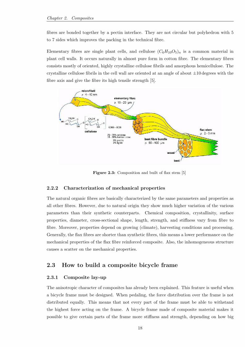
2.2.1 Structure and chemical composition
The main polymers involved in the composition of plant fibres are cellulose, hemicelluloses, lignin
and pectin. To understand the intricate structure of plant fibres, the flax fibre is considered
(figure 2.3). The approximately one meter long so-called technical fibres are isolated from the
flax plant for the use in textile industry. These technical fibres consist of elementary fibres with
lengths generally between 2 and 5 cm, and diameters between 10µm and 25µm. The elementary
17
Chapter 2. Composites
fibres are bonded together by a pectin interface. They are not circular but polyhedron with 5
to 7 sides which improves the packing in the technical fibre.
Elementary fibres are single plant cells, and cellulose (C6H10O5)n is a common material in
plant cell walls. It occurs naturally in almost pure form in cotton fibre. The elementary fibres
consists mostly of oriented, highly crystalline cellulose fibrils and amorphous hemicellulose. The
crystalline cellulose fibrils in the cell wall are oriented at an angle of about ±10 degrees with the
fibre axis and give the fibre its high tensile strength [5].
Figure 2.3: Composition and built of flax stem [5]
2.2.2 Characterization of mechanical properties
The natural organic fibres are basically characterized by the same parameters and properties as
all other fibres. However, due to natural origin they show much higher variation of the various
parameters than their synthetic counterparts. Chemical composition, crystallinity, surface
properties, diameter, cross-sectional shape, length, strength, and stiffness vary from fibre to
fibre. Moreover, properties depend on growing (climate), harvesting conditions and processing.
Generally, the flax fibres are shorter than synthetic fibres, this means a lower performance on the
mechanical properties of the flax fibre reinforced composite. Also, the inhomogeneous structure
causes a scatter on the mechanical properties.
2.3 How to build a composite bicycle frame
2.3.1 Composite lay-up
The anisotropic character of composites has already been explained. This feature is useful when
a bicycle frame must be designed. When pedaling, the force distribution over the frame is not
distributed equally. This means that not every part of the frame must be able to withstand
the highest force acting on the frame. A bicycle frame made of composite material makes it
possible to give certain parts of the frame more stiffness and strength, depending on how big
18
Chapter 2. Composites
the load is on that particular part. By applying different layers, each with a different (or the
same) direction of the fibres, more or less load can be sustained in a specific direction. As a
result thickness and fibre pattern can easily be changed all over the frame in order to achieve
the best results
2.3.2 Production process
The fibre reinforced polymers used for the bicycle frames are a combination of the resin (epoxy)
and the fibres (flax and carbon). In other words, the fibre is impregnated into the resin, this is
called a Pre-preg. Two sorts of pre-preg are used for the bicyle frames from Museeuw Bikes. The
first one is a pre-preg based on flax and epoxy, here the flax fibres all have the same direction.
This is called Uni Directional flax (flaxUD). The second kind of pre-preg is formed by a woven
pattern of flax and carbon fibre, impregnated into the epoxy resin. The thickness of such a
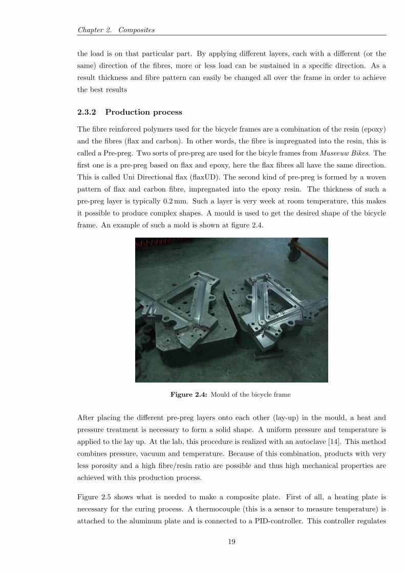
pre-preg layer is typically 0.2 mm. Such a layer is very week at room temperature, this makes
it possible to produce complex shapes. A mould is used to get the desired shape of the bicycle
frame. An example of such a mold is shown at figure 2.4.
Figure 2.4: Mould of the bicycle frame
After placing the different pre-preg layers onto each other (lay-up) in the mould, a heat and
pressure treatment is necessary to form a solid shape. A uniform pressure and temperature is
applied to the lay up. At the lab, this procedure is realized with an autoclave [14]. This method
combines pressure, vacuum and temperature. Because of this combination, products with very
less porosity and a high fibre/resin ratio are possible and thus high mechanical properties are
achieved with this production process.
Figure 2.5 shows what is needed to make a composite plate. First of all, a heating plate is
necessary for the curing process. A thermocouple (this is a sensor to measure temperature) is
attached to the aluminum plate and is connected to a PID-controller. This controller regulates
19
Chapter 2. Composites
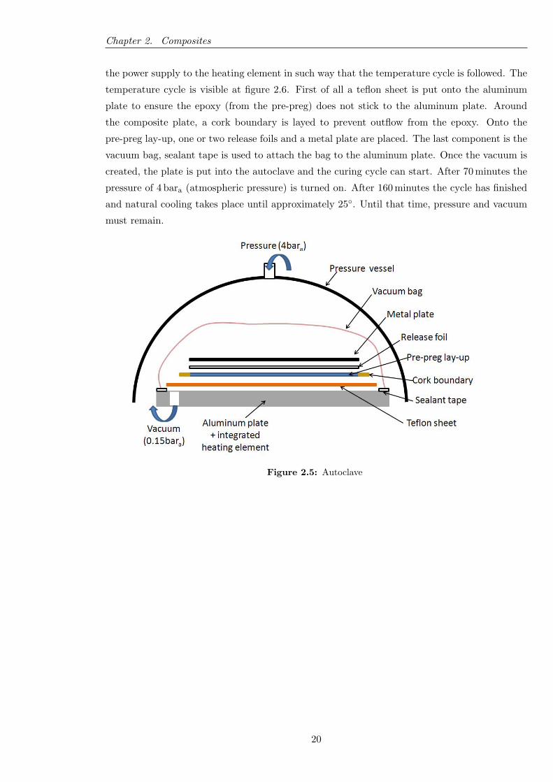
the power supply to the heating element in such way that the temperature cycle is followed. The
temperature cycle is visible at figure 2.6. First of all a teflon sheet is put onto the aluminum
plate to ensure the epoxy (from the pre-preg) does not stick to the aluminum plate. Around
the composite plate, a cork boundary is layed to prevent outflow from the epoxy. Onto the
pre-preg lay-up, one or two release foils and a metal plate are placed. The last component is the
vacuum bag, sealant tape is used to attach the bag to the aluminum plate. Once the vacuum is
created, the plate is put into the autoclave and the curing cycle can start. After 70 minutes the
pressure of 4 bara (atmospheric pressure) is turned on. After 160 minutes the cycle has finished
and natural cooling takes place until approximately 25◦. Until that time, pressure and vacuum
must remain.
Figure 2.5: Autoclave
20
Chapter 2. Composites
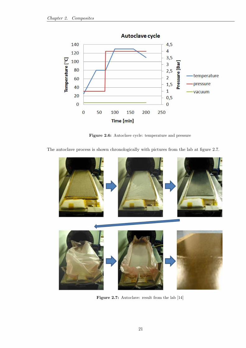
Figure 2.6: Autoclave cycle: temperature and pressure
The autoclave process is shown chronologically with pictures from the lab at figure 2.7.
Figure 2.7: Autoclave: result from the lab [14]
21

Chapter 3
Ride comfort and body vibration
3.1 Bicycle frames
New bicycle frame designs are generally motivated by weight, stiffness and comfort considerations
and often incorporate the use of high performance engineering materials. Indeed, competitive
cycling has promoted the use of various advanced structural materials including non-ferrous
alloys (primarily aluminum and titanium) and fibre reinforced polymers (e.g. carbon reinforced
epoxies). Both the frame design and material contribute to the rider’s energy consumption.
Energy is expended for propulsion and through elastic deformation of the frame. Therefore, a
minimization of the frame’s total mass and deflection are essential [15].
The ideal bicycle frame for a given rider would fit the rider’s body image and would be light. It
would absorb road shock well and the frame would deliver undiminished applied pedal power to
the chain sprocket at the rear wheel. It would be durable and not fail because of the continuous
pedaling load and would be strong enough to stand up to unexpected impacts and torsion forces.
It would lend itself to attractive finishing and would resist corrosion. Steel, titanium and carbon
fibre composites have the advantage over aluminum that there is a specific endurance limit
[16]. The endurance limit of a material is a mechanical property which is important when a
component is subjected to a time varying force. In case of a bicycle frame, the time varying
force is due to the crank rotations. When a material has a endurance limit than it does not
matter how many crank rotations the frame is subjected to, the frame will never fail because of
exceeding the fatigue life of the material. In case of an aluminum frame, when enough (read:
very much) crank rotations have passed the frame will fail.
Vibration and shock damping are two important factors that affect the cyclist. However, they are
two of the least understood subjects in materials science. There are so many variables involved,
for instance how atoms in a material absorb and dissipate vibration energy, how the structure is
built, what type of paint and plating are applied,... that it is hard to predict how a structure will
react to vibration input. Damping measures the rate at which vibrations dissipate. Damping
gives a vibration-free ride, as road shock vanishes within the frame. For cyclists, this translates
22
Chapter 3. Ride comfort and body vibration
to a smoother and longer ride with less fatigue of the cyclist [17]. Composite’s vibration damping
is far superior to any metal, which is why it is the preferred material for race car springs and
high performance airplanes [16]. The smooth ride quality is one of the first things people notice
about composite bicycle frames.
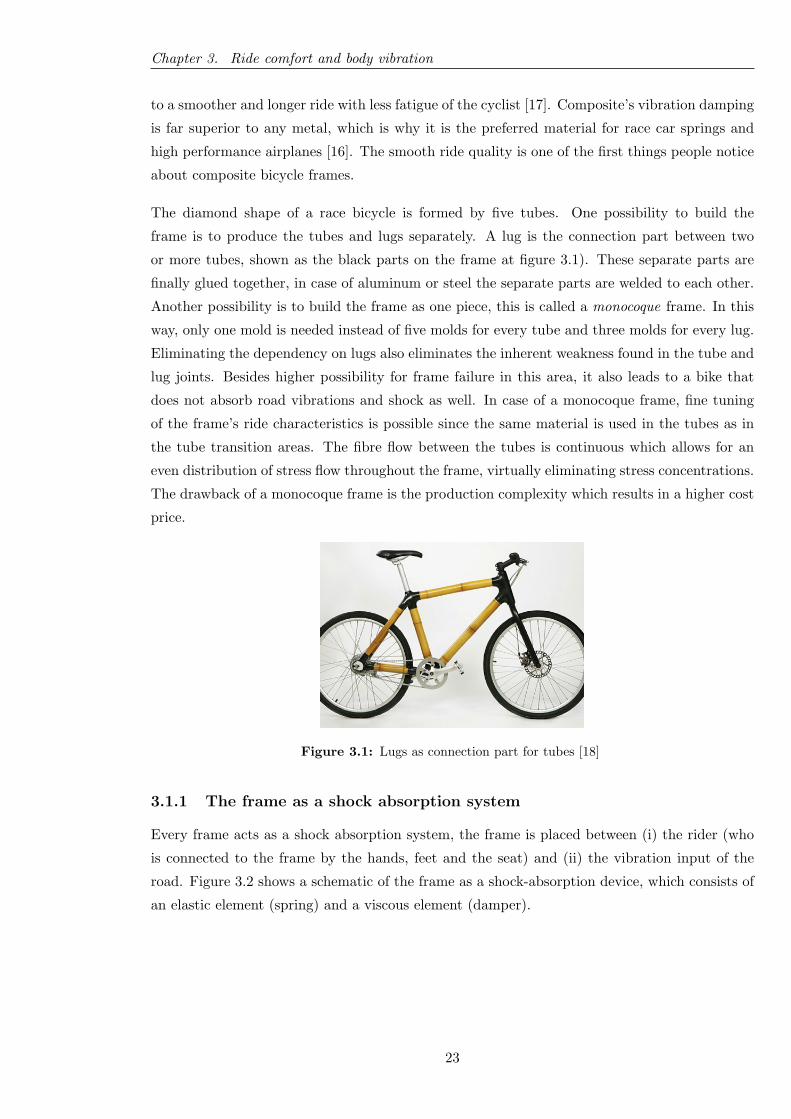
The diamond shape of a race bicycle is formed by five tubes. One possibility to build the
frame is to produce the tubes and lugs separately. A lug is the connection part between two
or more tubes, shown as the black parts on the frame at figure 3.1). These separate parts are
finally glued together, in case of aluminum or steel the separate parts are welded to each other.
Another possibility is to build the frame as one piece, this is called a monocoque frame. In this
way, only one mold is needed instead of five molds for every tube and three molds for every lug.
Eliminating the dependency on lugs also eliminates the inherent weakness found in the tube and
lug joints. Besides higher possibility for frame failure in this area, it also leads to a bike that
does not absorb road vibrations and shock as well. In case of a monocoque frame, fine tuning
of the frame’s ride characteristics is possible since the same material is used in the tubes as in
the tube transition areas. The fibre flow between the tubes is continuous which allows for an
even distribution of stress flow throughout the frame, virtually eliminating stress concentrations.
The drawback of a monocoque frame is the production complexity which results in a higher cost
price.
Figure 3.1: Lugs as connection part for tubes [18]
3.1.1 The frame as a shock absorption system
Every frame acts as a shock absorption system, the frame is placed between (i) the rider (who
is connected to the frame by the hands, feet and the seat) and (ii) the vibration input of the
road. Figure 3.2 shows a schematic of the frame as a shock-absorption device, which consists of
an elastic element (spring) and a viscous element (damper).
23

Chapter 3. Ride comfort and body vibration
Figure 3.2: The frame as a shock-absorption device [16]
The vibration input comes from the imperfection of the road surface. These imperfections are
transmitted by the spokes to the shaft of each wheel, the shafts are connected with the frame
so each vibration on the shaft is put directly to the frame. A part of the vibration is already
absorbed by the tire, the rim and the spokes. These three parameters can be adapted to minimize
the vibration (or maximize the comfort of the rider) due to the road roughness. However, a lot
of vibration is still present at the point where shaft and frame are attached, so the vibration
can now only be reduced by adjusting the frame. Figure 3.3 depicts the forces which interact
with the frame. These can be classified in two categories (a) forces generated by the terrain
irregularities; and (b) forces generated by the movement of the cyclist which are applied to the
handlebar, saddle and pedals.
Figure 3.3: Forces transmitted to the frame [16]
All the vibration energy which cannot be absorbed by the bike will be dissipated by the body
parts of the cyclist. Changing the frame geometry is a possibility, by including locations which
flex relatively more compared to other ones due to the rider’s weight or applied forces. These
deformations give the rider more comfort. But also using a new frame material could improve
the ride comfort. Composites are preferred over steel, aluminum and titanium because of the
24
Chapter 3. Ride comfort and body vibration
improvement of shock absorption.
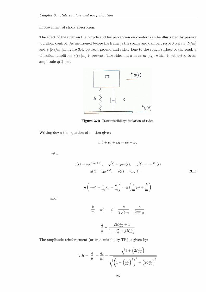
The effect of the rider on the bicycle and his perception on comfort can be illustrated by passive
vibration control. As mentioned before the frame is the spring and damper, respectively k [N/m]
and c [Ns/m ]at figure 3.4, between ground and rider. Due to the rough surface of the road, a
vibration amplitude y(t) [m] is present. The rider has a mass m [kg], which is subjected to an
amplitude q(t) [m].
Figure 3.4: Transmissibility: isolation of rider
Writing down the equation of motion gives:
mq + cq + kq = cy + ky
with:
q(t) = q0ej(ωt+φ), ˙q(t) = jωq(t), ¨q(t) = −ω2q(t)
y(t) = y0ejωt, ˙y(t) = jωy(t), (3.1)
q
(−ω2 +
c
mjω +
k
m
)= y
(c
mjω +
k
m
)and:
k
m= ω2
n, ζ =c
2√km
=c
2mωn
q
y=
j2ζ ωωn
+ 1
1− ω2
ω2n
+ j2ζ ωωn
The amplitude reinforcement (or transmissibility TR) is given by:
TR =∣∣∣∣qy∣∣∣∣ =
q0
y0=
√1 +
(2ζ ω
ωn
)√(
1−(ωωn
)2)2
+(
2ζ ωωn
)2
25
Chapter 3. Ride comfort and body vibration
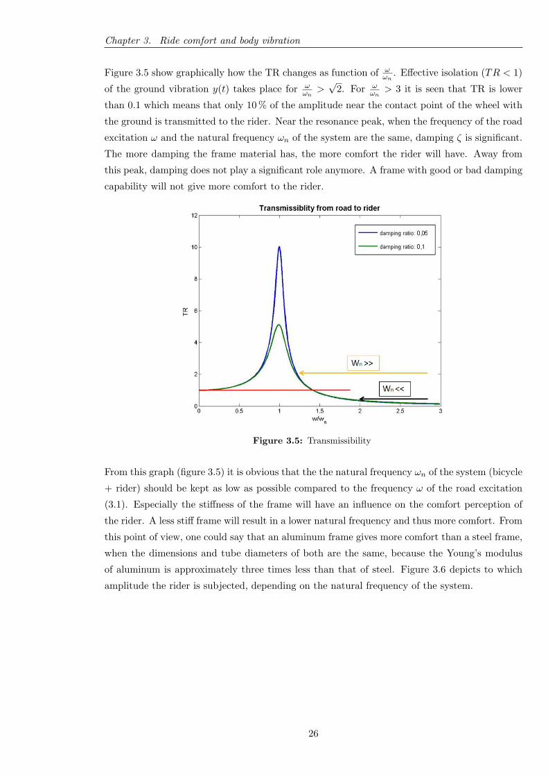
Figure 3.5 show graphically how the TR changes as function of ωωn
. Effective isolation (TR < 1)
of the ground vibration y(t) takes place for ωωn
>√
2. For ωωn
> 3 it is seen that TR is lower
than 0.1 which means that only 10 % of the amplitude near the contact point of the wheel with
the ground is transmitted to the rider. Near the resonance peak, when the frequency of the road
excitation ω and the natural frequency ωn of the system are the same, damping ζ is significant.
The more damping the frame material has, the more comfort the rider will have. Away from
this peak, damping does not play a significant role anymore. A frame with good or bad damping
capability will not give more comfort to the rider.
Figure 3.5: Transmissibility
From this graph (figure 3.5) it is obvious that the the natural frequency ωn of the system (bicycle
+ rider) should be kept as low as possible compared to the frequency ω of the road excitation
(3.1). Especially the stiffness of the frame will have an influence on the comfort perception of
the rider. A less stiff frame will result in a lower natural frequency and thus more comfort. From
this point of view, one could say that an aluminum frame gives more comfort than a steel frame,
when the dimensions and tube diameters of both are the same, because the Young’s modulus
of aluminum is approximately three times less than that of steel. Figure 3.6 depicts to which
amplitude the rider is subjected, depending on the natural frequency of the system.
26

Chapter 3. Ride comfort and body vibration
Figure 3.6: Transmissiblity: influence of natural frequency
Very important here to note is that only one natural frequency of the system (bicycle +
rider) is considered and just one excitation frequency (coming from the road) occurs. In reality
a whole different situations takes place. On the one side, the road excitation is a broadband
signal, which means that a lot of frequencies occur. On the other side, the system has several
natural frequencies. If this situation should take place, it can be something as shown at figure
3.7. Here, damping of the frame cannot be neglected anymore since resonance peaks are found
over a wide range in the frequency domain.
Figure 3.7: Transmissiblity: real situation. Blue: ζ = 2%, Green: ζ = 4%
27
Chapter 3. Ride comfort and body vibration
3.1.2 Shock absorption versus energy loss
Every vibration and shock to the human body must be compensated by muscular strength, which
over long distances produces fatigue of the cyclist. However, no power should be absorbed by
the damping/suspension of the frame.
When riding on a bicycle, inevitable the frame will deform. This elastic deformation of the
frame comes from energy expended by the rider. Building a frame which has better damping
characteristics is twofold. On the one hand the terrain-induced energy is dissipated in a better
way resulting in smaller vibrations at the contact points of the rider with the frame, which
results in improved comfort and handling. A better damping may also improve cornering,
braking capacity, and more generally, bicycle control, handling and traction since they allow
better contact between the tyres and the ground. On the other hand, the frame may also
dissipate the cyclist’s energy through small oscillatory movements, often termed ’bobbing’ [16],
which are generated by (i) the displacement of the cyclist’s body parts; and (ii) the interaction
between the forces applied on the pedals which are transmitted to the frame.
An investigation on the physiological and perceptual responses of adding vibration to cycling
[19] yielded more absolute and relative oxygen intake values and minute ventilation (the volume
of air which can be inhaled per minute) during cycling at 250 and 300 Watts with vibration
when compared to the trials without vibration. Another study [20] found similar results as
the previous one, a body that is subjected to vibrations cannot perform the same as it would
be without this vibration. All these findings show that a superimposed vibration stimulus on
cycling plays a role in designing bicycle frames. Any improvement in reducing the road vibration
should result in a better performance of the cyclist.
The effect of suspension systems on the comfort and energy loss has already been studied for
off-road bicycles [16]. The study evaluated the oxygen consumption (V O2) of cyclists riding
different types of bicycles (no -, front -and full suspension) and found no significant increase in
energy expended by the cyclist riding on a smooth surface. The full suspension allowed a 11, 5 %
decrease in V O2 compared with the non-suspended condition when riding on a rough surface.
A conclusion that counts for the different studies [2, 3] is that the magnitude of any energy
dissipation by a suspension system must by very small, if any, and thus probably negligible
compared with the advantages they provide.
3.1.3 Designing a bicycle frame
Intuition and trial-and-error have played major roles in the evolution of today’s diamond-shaped
composite frames. The design and manufacture of bicycle frames has largely been an art,
performed by skilled craftsmen; their efforts have resulted in reliable, efficient structures.
The limitations of trial-and-error become most apparent when new materials enter the picture,
and when new applications and demands are placed on the structure. Trial-and-error is costly
28
Chapter 3. Ride comfort and body vibration
and slow, and intuition does not always yield reliable results. A solution for this problem is the
Finite-Element Analysis method (FEA). Based on computer calculations the frame geometry
and tubes can be optimized. The inputs needed to perform such analysis are the frame’s
geometry, boundary conditions (how is the frame connected with the ground) and loads (impact,
braking and pedaling). The output can be stress, strain, etc.
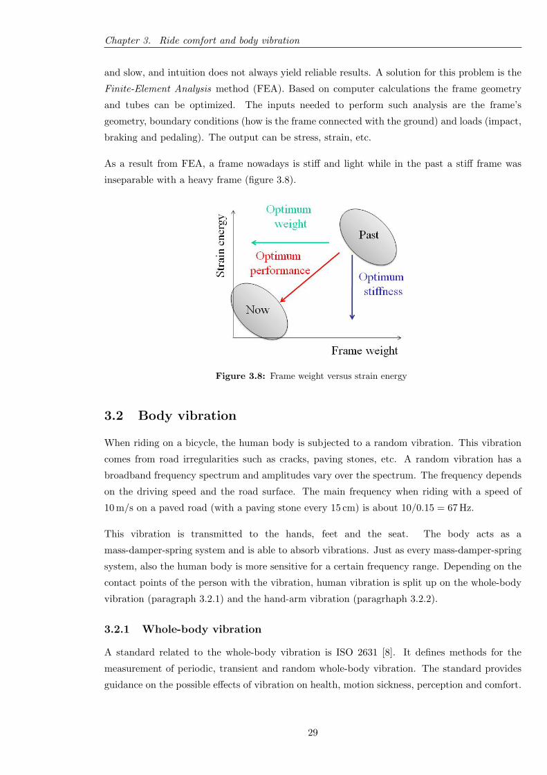
As a result from FEA, a frame nowadays is stiff and light while in the past a stiff frame was
inseparable with a heavy frame (figure 3.8).
Figure 3.8: Frame weight versus strain energy
3.2 Body vibration
When riding on a bicycle, the human body is subjected to a random vibration. This vibration
comes from road irregularities such as cracks, paving stones, etc. A random vibration has a
broadband frequency spectrum and amplitudes vary over the spectrum. The frequency depends
on the driving speed and the road surface. The main frequency when riding with a speed of
10 m/s on a paved road (with a paving stone every 15 cm) is about 10/0.15 = 67 Hz.
This vibration is transmitted to the hands, feet and the seat. The body acts as a
mass-damper-spring system and is able to absorb vibrations. Just as every mass-damper-spring
system, also the human body is more sensitive for a certain frequency range. Depending on the
contact points of the person with the vibration, human vibration is split up on the whole-body
vibration (paragraph 3.2.1) and the hand-arm vibration (paragrhaph 3.2.2).
3.2.1 Whole-body vibration
A standard related to the whole-body vibration is ISO 2631 [8]. It defines methods for the
measurement of periodic, transient and random whole-body vibration. The standard provides
guidance on the possible effects of vibration on health, motion sickness, perception and comfort.
29
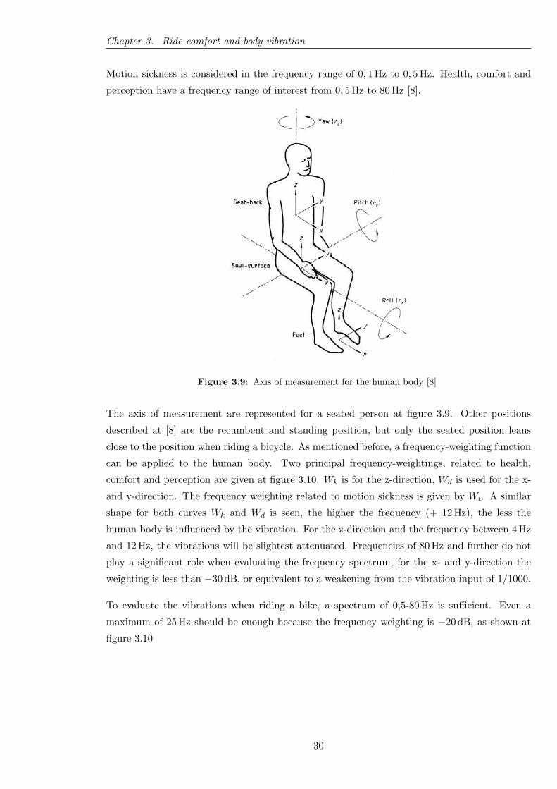
Chapter 3. Ride comfort and body vibration
Motion sickness is considered in the frequency range of 0, 1 Hz to 0, 5 Hz. Health, comfort and
perception have a frequency range of interest from 0, 5 Hz to 80 Hz [8].
Figure 3.9: Axis of measurement for the human body [8]
The axis of measurement are represented for a seated person at figure 3.9. Other positions
described at [8] are the recumbent and standing position, but only the seated position leans
close to the position when riding a bicycle. As mentioned before, a frequency-weighting function
can be applied to the human body. Two principal frequency-weightings, related to health,
comfort and perception are given at figure 3.10. Wk is for the z-direction, Wd is used for the x-
and y-direction. The frequency weighting related to motion sickness is given by Wt. A similar
shape for both curves Wk and Wd is seen, the higher the frequency (+ 12 Hz), the less the
human body is influenced by the vibration. For the z-direction and the frequency between 4 Hz
and 12 Hz, the vibrations will be slightest attenuated. Frequencies of 80 Hz and further do not
play a significant role when evaluating the frequency spectrum, for the x- and y-direction the
weighting is less than −30 dB, or equivalent to a weakening from the vibration input of 1/1000.
To evaluate the vibrations when riding a bike, a spectrum of 0,5-80 Hz is sufficient. Even a
maximum of 25 Hz should be enough because the frequency weighting is −20 dB, as shown at
figure 3.10
30
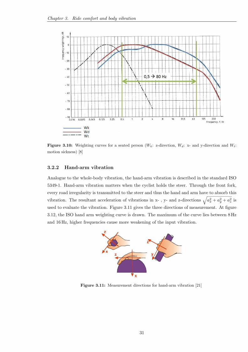
Chapter 3. Ride comfort and body vibration
Figure 3.10: Weighting curves for a seated person (Wk: z-direction, Wd: x- and y-direction and Wt:
motion sickness) [8]
3.2.2 Hand-arm vibration
Analogue to the whole-body vibration, the hand-arm vibration is described in the standard ISO
5349-1. Hand-arm vibration matters when the cyclist holds the steer. Through the front fork,
every road irregularity is transmitted to the steer and thus the hand and arm have to absorb this
vibration. The resultant acceleration of vibrations in x- , y- and z-directions√a2x + a2
y + a2z is
used to evaluate the vibration. Figure 3.11 gives the three directions of measurement. At figure
3.12, the ISO hand arm weighting curve is drawn. The maximum of the curve lies between 8 Hz
and 16 Hz, higher frequencies cause more weakening of the input vibration.
Figure 3.11: Measurement directions for hand-arm vibration [21]
31
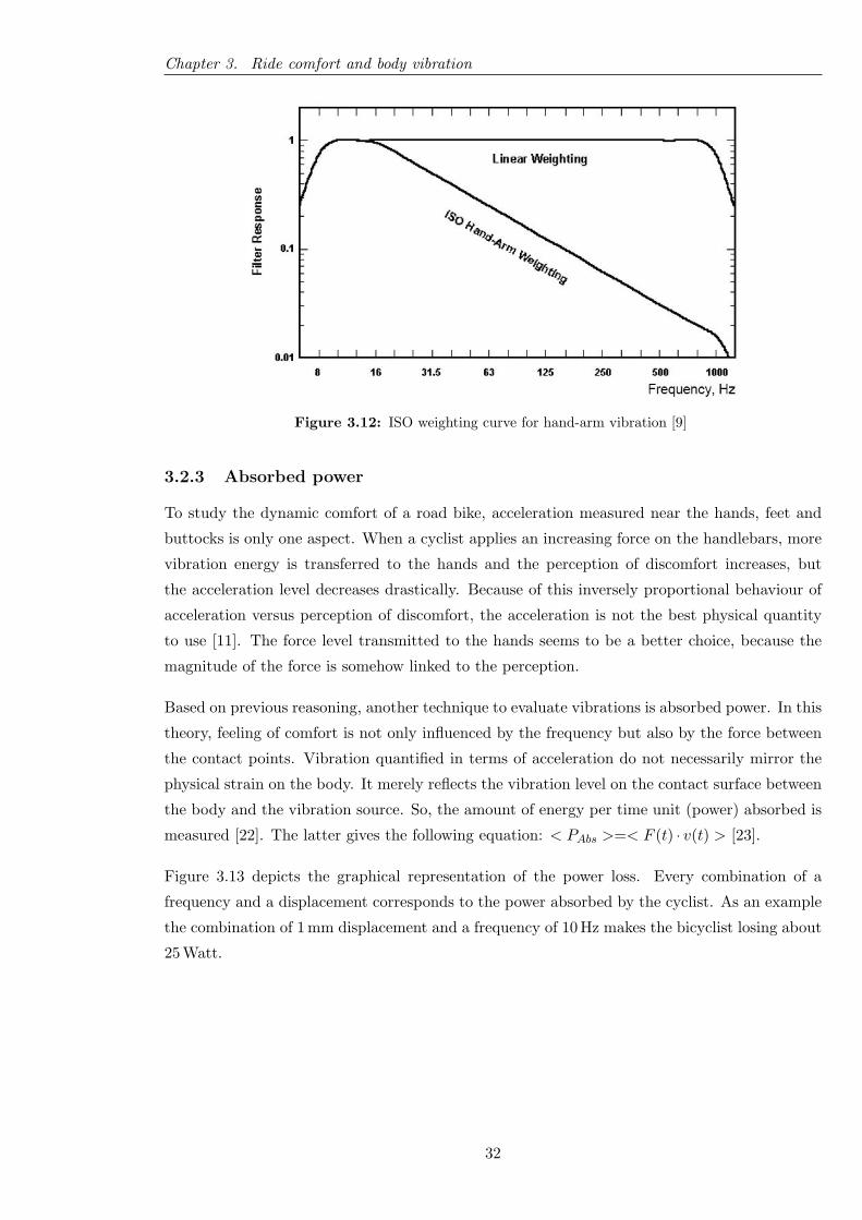
Chapter 3. Ride comfort and body vibration
Figure 3.12: ISO weighting curve for hand-arm vibration [9]
3.2.3 Absorbed power
To study the dynamic comfort of a road bike, acceleration measured near the hands, feet and
buttocks is only one aspect. When a cyclist applies an increasing force on the handlebars, more
vibration energy is transferred to the hands and the perception of discomfort increases, but
the acceleration level decreases drastically. Because of this inversely proportional behaviour of
acceleration versus perception of discomfort, the acceleration is not the best physical quantity
to use [11]. The force level transmitted to the hands seems to be a better choice, because the
magnitude of the force is somehow linked to the perception.
Based on previous reasoning, another technique to evaluate vibrations is absorbed power. In this
theory, feeling of comfort is not only influenced by the frequency but also by the force between
the contact points. Vibration quantified in terms of acceleration do not necessarily mirror the
physical strain on the body. It merely reflects the vibration level on the contact surface between
the body and the vibration source. So, the amount of energy per time unit (power) absorbed is
measured [22]. The latter gives the following equation: < PAbs >=< F (t) · v(t) > [23].
Figure 3.13 depicts the graphical representation of the power loss. Every combination of a
frequency and a displacement corresponds to the power absorbed by the cyclist. As an example
the combination of 1 mm displacement and a frequency of 10 Hz makes the bicyclist losing about
25 Watt.
32
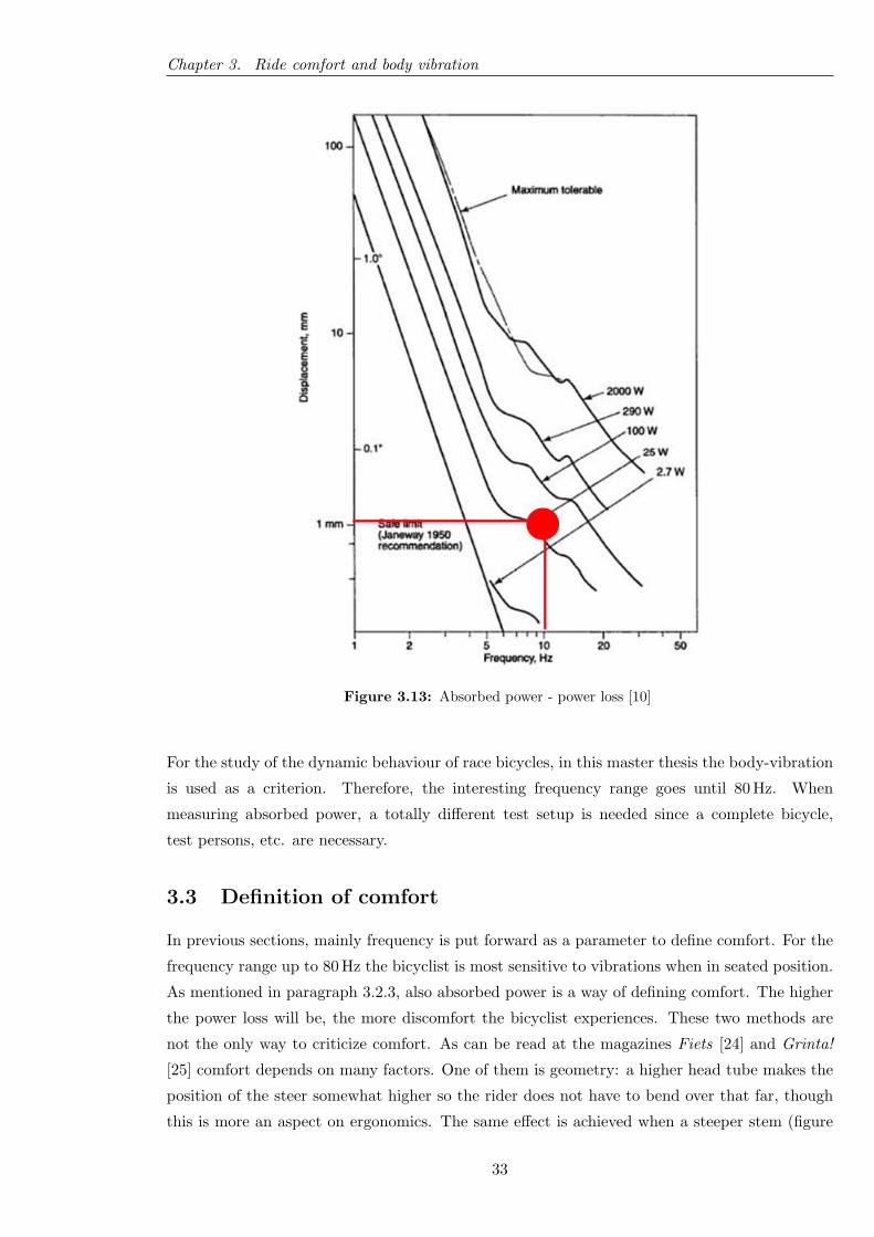
Chapter 3. Ride comfort and body vibration
Figure 3.13: Absorbed power - power loss [10]
For the study of the dynamic behaviour of race bicycles, in this master thesis the body-vibration
is used as a criterion. Therefore, the interesting frequency range goes until 80 Hz. When
measuring absorbed power, a totally different test setup is needed since a complete bicycle,
test persons, etc. are necessary.
3.3 Definition of comfort
In previous sections, mainly frequency is put forward as a parameter to define comfort. For the
frequency range up to 80 Hz the bicyclist is most sensitive to vibrations when in seated position.
As mentioned in paragraph 3.2.3, also absorbed power is a way of defining comfort. The higher
the power loss will be, the more discomfort the bicyclist experiences. These two methods are
not the only way to criticize comfort. As can be read at the magazines Fiets [24] and Grinta!
[25] comfort depends on many factors. One of them is geometry: a higher head tube makes the
position of the steer somewhat higher so the rider does not have to bend over that far, though
this is more an aspect on ergonomics. The same effect is achieved when a steeper stem (figure
33
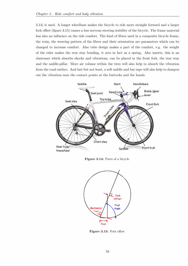
Chapter 3. Ride comfort and body vibration
3.14) is used. A longer wheelbase makes the bicycle to ride more straight forward and a larger
fork offset (figure 3.15) causes a less nervous steering stability of the bicycle. The frame material
has also an influence on the ride comfort. The kind of fibres used in a composite bicycle frame,
the resin, the weaving pattern of the fibres and their orientation are parameters which can be
changed to increase comfort. Also tube design makes a part of the comfort, e.g. the weight
of the rider makes the rear stay bending, it acts in fact as a spring. Also inserts, this is an
elastomer which absorbs shocks and vibrations, can be placed in the front fork, the rear stay
and the saddle-pillar. More air volume within the tires will also help to absorb the vibration
form the road surface. And last but not least, a soft saddle and bar tape will also help to dampen
out the vibration near the contact points at the buttocks and the hands.
Figure 3.14: Parts of a bicycle
Figure 3.15: Fork offset
34
Chapter 4
Vibration analysis on isotropic and
orthotropic materials
4.1 Introduction
From the previous chapter it is seen that comfort depends on many factors, one of them is the
vibration. To analyze how a bicycle frame reacts on this vibration, modal analysis is a technique
to get the characteristics from the frame. How the frame reacts onto an input force with varying
frequency is than examined. As a first step to get used to modal analysis, vibration testing has
been done on simple structure such as a beam. Once this succeeds, it is possible to subject a
complex geometry (the flax-carbon reinforced composite frames) to vibration testing.
4.2 Modal analysis explained in a nutshell
To fully understand what is meant with vibration analysis, some theory about modal analysis is
necessary. At this moment, only the basic idea behind it is explained while at the next chapter
more explanation is given.
Modal analysis is a process whereby the structure is described in terms of its natural
characteristics which are the frequency, damping and mode shapes. These three are called the
dynamic properties from a structure. Modal analysis can best be explained by an example. At
a freely supported flat plate (figure 4.1) a force is applied to one corner of the plate. The force
has a constant amplitude, but the force varies in a sinusoidal fashion. The rate of oscillation of
the frequency is swept up from a low to a high frequency. Also the response of the plate due to
the excitation is measured, this is done by means of an acceleration sensor (accelerometer).
35
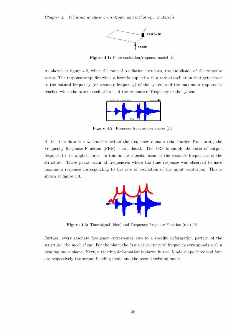
Chapter 4. Vibration analysis on isotropic and orthotropic materials
Figure 4.1: Plate excitation/response model [26]
As shown at figure 4.2, when the rate of oscillation increases, the amplitude of the response
varies. The response amplifies when a force is applied with a rate of oscillation that gets closer
to the natural frequency (or resonate frequency) of the system and the maximum response is
reached when the rate of oscillation is at the resonate of frequency of the system.
Figure 4.2: Response from accelerometer [26]
If the time data is now transformed to the frequency domain (via Fourier Transform), the
Frequency Response Function (FRF) is calculated. The FRF is simply the ratio of output
response to the applied force. In this function peaks occur at the resonate frequencies of the
structure. These peaks occur at frequencies where the time response was observed to have
maximum response corresponding to the rate of oscillation of the input excitation. This is
shown at figure 4.3.
Figure 4.3: Time signal (blue) and Frequency Response Function (red) [26]
Further, every resonate frequency corresponds also to a specific deformation pattern of the
structure: the mode shape. For the plate, the first natural natural frequency corresponds with a
bending mode shape. Next, a twisting deformation is shown in red. Mode shape three and four
are respectively the second bending mode and the second twisting mode.
36
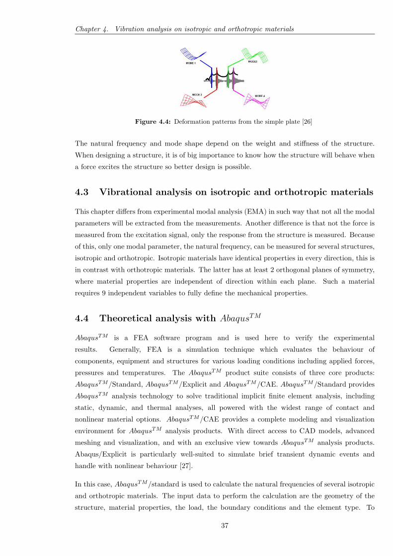
Chapter 4. Vibration analysis on isotropic and orthotropic materials
Figure 4.4: Deformation patterns from the simple plate [26]
The natural frequency and mode shape depend on the weight and stiffness of the structure.
When designing a structure, it is of big importance to know how the structure will behave when
a force excites the structure so better design is possible.
4.3 Vibrational analysis on isotropic and orthotropic materials
This chapter differs from experimental modal analysis (EMA) in such way that not all the modal
parameters will be extracted from the measurements. Another difference is that not the force is
measured from the excitation signal, only the response from the structure is measured. Because
of this, only one modal parameter, the natural frequency, can be measured for several structures,
isotropic and orthotropic. Isotropic materials have identical properties in every direction, this is
in contrast with orthotropic materials. The latter has at least 2 orthogonal planes of symmetry,
where material properties are independent of direction within each plane. Such a material
requires 9 independent variables to fully define the mechanical properties.
4.4 Theoretical analysis with AbaqusTM
AbaqusTM is a FEA software program and is used here to verify the experimental
results. Generally, FEA is a simulation technique which evaluates the behaviour of
components, equipment and structures for various loading conditions including applied forces,
pressures and temperatures. The AbaqusTM product suite consists of three core products:
AbaqusTM/Standard, AbaqusTM/Explicit and AbaqusTM/CAE. AbaqusTM/Standard provides
AbaqusTM analysis technology to solve traditional implicit finite element analysis, including
static, dynamic, and thermal analyses, all powered with the widest range of contact and
nonlinear material options. AbaqusTM/CAE provides a complete modeling and visualization
environment for AbaqusTM analysis products. With direct access to CAD models, advanced
meshing and visualization, and with an exclusive view towards AbaqusTM analysis products.
Abaqus/Explicit is particularly well-suited to simulate brief transient dynamic events and
handle with nonlinear behaviour [27].
In this case, AbaqusTM/standard is used to calculate the natural frequencies of several isotropic
and orthotropic materials. The input data to perform the calculation are the geometry of the
structure, material properties, the load, the boundary conditions and the element type. To
37
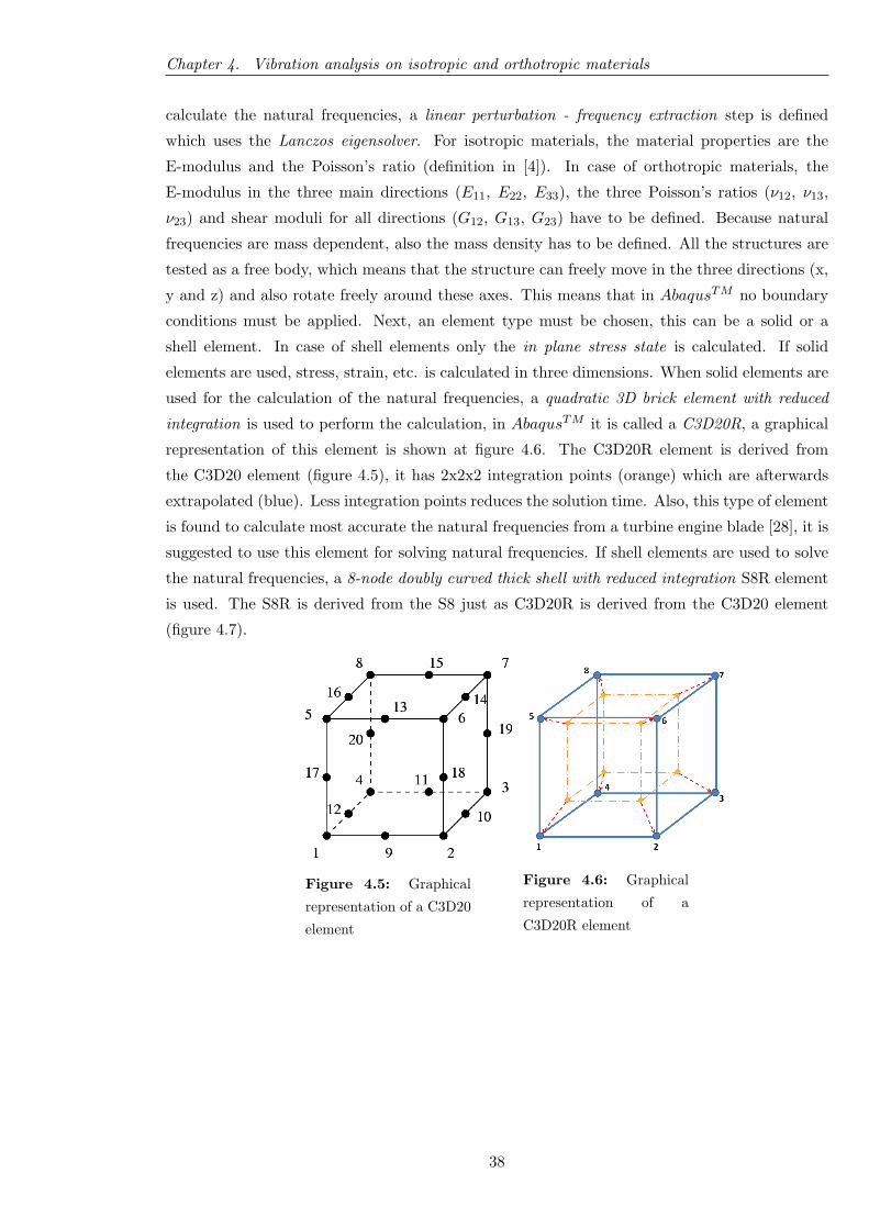
Chapter 4. Vibration analysis on isotropic and orthotropic materials
calculate the natural frequencies, a linear perturbation - frequency extraction step is defined
which uses the Lanczos eigensolver. For isotropic materials, the material properties are the
E-modulus and the Poisson’s ratio (definition in [4]). In case of orthotropic materials, the
E-modulus in the three main directions (E11, E22, E33), the three Poisson’s ratios (ν12, ν13,
ν23) and shear moduli for all directions (G12, G13, G23) have to be defined. Because natural
frequencies are mass dependent, also the mass density has to be defined. All the structures are
tested as a free body, which means that the structure can freely move in the three directions (x,
y and z) and also rotate freely around these axes. This means that in AbaqusTM no boundary
conditions must be applied. Next, an element type must be chosen, this can be a solid or a
shell element. In case of shell elements only the in plane stress state is calculated. If solid
elements are used, stress, strain, etc. is calculated in three dimensions. When solid elements are
used for the calculation of the natural frequencies, a quadratic 3D brick element with reduced
integration is used to perform the calculation, in AbaqusTM it is called a C3D20R, a graphical
representation of this element is shown at figure 4.6. The C3D20R element is derived from
the C3D20 element (figure 4.5), it has 2x2x2 integration points (orange) which are afterwards
extrapolated (blue). Less integration points reduces the solution time. Also, this type of element
is found to calculate most accurate the natural frequencies from a turbine engine blade [28], it is
suggested to use this element for solving natural frequencies. If shell elements are used to solve
the natural frequencies, a 8-node doubly curved thick shell with reduced integration S8R element
is used. The S8R is derived from the S8 just as C3D20R is derived from the C3D20 element
(figure 4.7).
Figure 4.5: Graphical
representation of a C3D20
element
Figure 4.6: Graphical
representation of a
C3D20R element
38
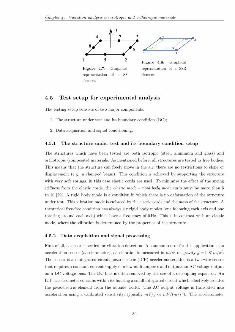
Chapter 4. Vibration analysis on isotropic and orthotropic materials
Figure 4.7: Graphical
representation of a S8
element
Figure 4.8: Graphical
representation of a S8R
element
4.5 Test setup for experimental analysis
The testing setup consists of two major components.
1. The structure under test and its boundary condition (BC);
2. Data acquisition and signal conditioning.
4.5.1 The structure under test and its boundary condition setup
The structures which have been tested are both isotropic (steel, aluminum and glass) and
orthotropic (composite) materials. As mentioned before, all structures are tested as free bodies.
This means that the structure can freely move in the air, there are no restrictions to slope or
displacement (e.g. a clamped beam). This condition is achieved by supporting the structure
with very soft springs, in this case elastic cords are used. To minimize the effect of the spring
stiffness from the elastic cords, the elastic mode - rigid body mode ratio must be more than 5
to 10 [29]. A rigid body mode is a condition in which there is no deformation of the structure
under test. This vibration mode is enforced by the elastic cords and the mass of the structure. A
theoretical free-free condition has always six rigid body modes (one following each axis and one
rotating around each axis) which have a frequency of 0 Hz. This is in contrast with an elastic
mode, where the vibration is determined by the properties of the structure.
4.5.2 Data acquisition and signal processing
First of all, a sensor is needed for vibration detection. A common sensor for this application is an
acceleration sensor (accelerometer), acceleration is measured in m/s2 or gravity g = 9.81m/s2.
The sensor is an integrated circuit-piezo electric (ICP) accelerometer, this is a two-wire sensor
that requires a constant current supply of a few milli-amperes and outputs an AC voltage output
on a DC voltage bias. The DC bias is often removed by the use of a decoupling capacitor. An
ICP accelerometer contains within its housing a small integrated circuit which effectively isolates
the piezoelectric element from the outside world. The AC output voltage is translated into
acceleration using a calibrated sensitivity, typically mV/g or mV/(m/s2). The accelerometer
39
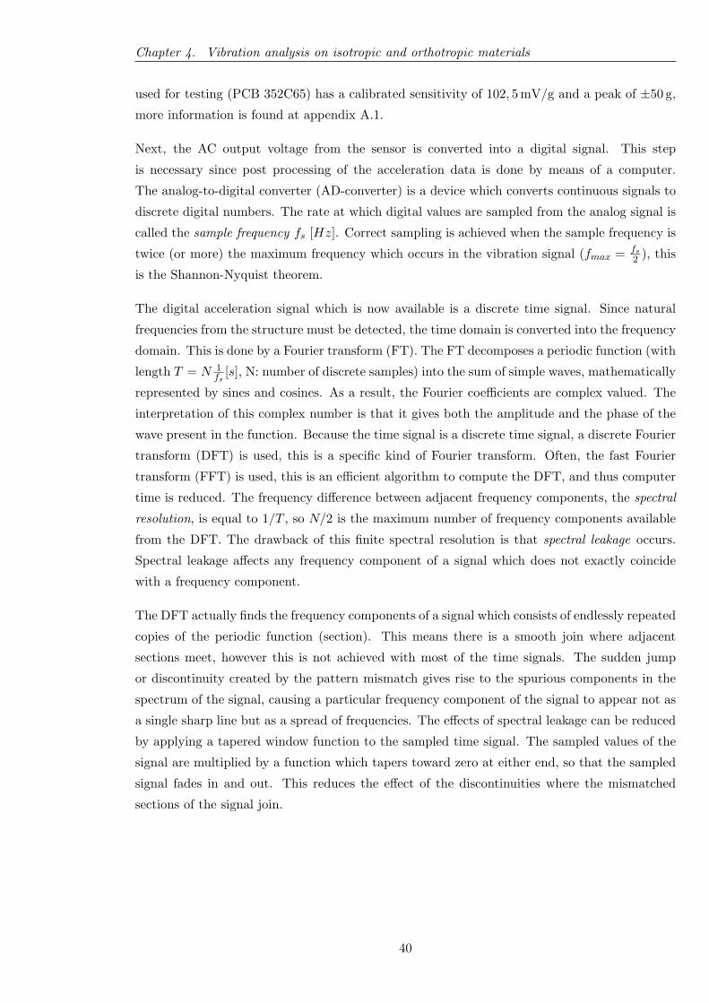
Chapter 4. Vibration analysis on isotropic and orthotropic materials
used for testing (PCB 352C65) has a calibrated sensitivity of 102, 5 mV/g and a peak of ±50 g,
more information is found at appendix A.1.
Next, the AC output voltage from the sensor is converted into a digital signal. This step
is necessary since post processing of the acceleration data is done by means of a computer.
The analog-to-digital converter (AD-converter) is a device which converts continuous signals to
discrete digital numbers. The rate at which digital values are sampled from the analog signal is
called the sample frequency fs [Hz]. Correct sampling is achieved when the sample frequency is
twice (or more) the maximum frequency which occurs in the vibration signal (fmax = fs
2 ), this
is the Shannon-Nyquist theorem.
The digital acceleration signal which is now available is a discrete time signal. Since natural
frequencies from the structure must be detected, the time domain is converted into the frequency
domain. This is done by a Fourier transform (FT). The FT decomposes a periodic function (with
length T = N 1fs
[s], N: number of discrete samples) into the sum of simple waves, mathematically
represented by sines and cosines. As a result, the Fourier coefficients are complex valued. The
interpretation of this complex number is that it gives both the amplitude and the phase of the
wave present in the function. Because the time signal is a discrete time signal, a discrete Fourier
transform (DFT) is used, this is a specific kind of Fourier transform. Often, the fast Fourier
transform (FFT) is used, this is an efficient algorithm to compute the DFT, and thus computer
time is reduced. The frequency difference between adjacent frequency components, the spectral
resolution, is equal to 1/T , so N/2 is the maximum number of frequency components available
from the DFT. The drawback of this finite spectral resolution is that spectral leakage occurs.
Spectral leakage affects any frequency component of a signal which does not exactly coincide
with a frequency component.
The DFT actually finds the frequency components of a signal which consists of endlessly repeated
copies of the periodic function (section). This means there is a smooth join where adjacent
sections meet, however this is not achieved with most of the time signals. The sudden jump
or discontinuity created by the pattern mismatch gives rise to the spurious components in the
spectrum of the signal, causing a particular frequency component of the signal to appear not as
a single sharp line but as a spread of frequencies. The effects of spectral leakage can be reduced
by applying a tapered window function to the sampled time signal. The sampled values of the
signal are multiplied by a function which tapers toward zero at either end, so that the sampled
signal fades in and out. This reduces the effect of the discontinuities where the mismatched
sections of the signal join.
40
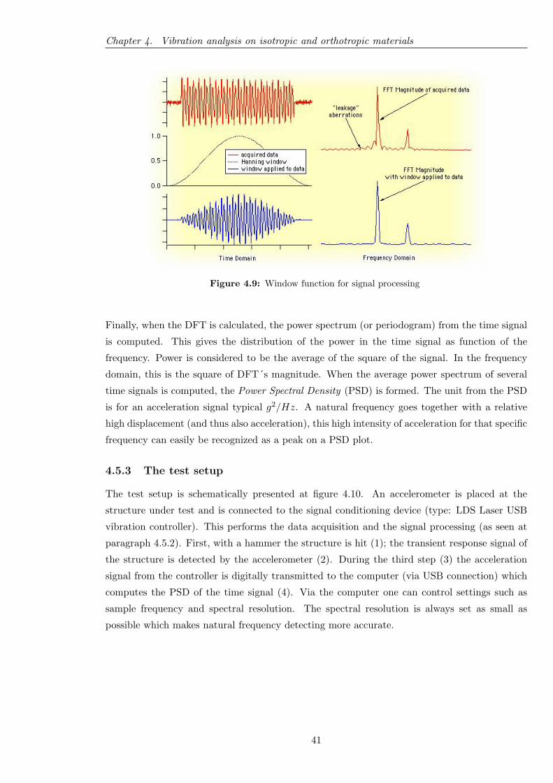
Chapter 4. Vibration analysis on isotropic and orthotropic materials
Figure 4.9: Window function for signal processing
Finally, when the DFT is calculated, the power spectrum (or periodogram) from the time signal
is computed. This gives the distribution of the power in the time signal as function of the
frequency. Power is considered to be the average of the square of the signal. In the frequency
domain, this is the square of DFT´s magnitude. When the average power spectrum of several
time signals is computed, the Power Spectral Density (PSD) is formed. The unit from the PSD
is for an acceleration signal typical g2/Hz. A natural frequency goes together with a relative
high displacement (and thus also acceleration), this high intensity of acceleration for that specific
frequency can easily be recognized as a peak on a PSD plot.
4.5.3 The test setup
The test setup is schematically presented at figure 4.10. An accelerometer is placed at the
structure under test and is connected to the signal conditioning device (type: LDS Laser USB
vibration controller). This performs the data acquisition and the signal processing (as seen at
paragraph 4.5.2). First, with a hammer the structure is hit (1); the transient response signal of
the structure is detected by the accelerometer (2). During the third step (3) the acceleration
signal from the controller is digitally transmitted to the computer (via USB connection) which
computes the PSD of the time signal (4). Via the computer one can control settings such as
sample frequency and spectral resolution. The spectral resolution is always set as small as
possible which makes natural frequency detecting more accurate.
41

Chapter 4. Vibration analysis on isotropic and orthotropic materials
Figure 4.10: Test setup for vibration testing
4.6 Vibration testing on isotropic material
4.6.1 Steel beam
Theoretical analysis
The dimensions of the steel beam are 760x50x4 mm and with a mass density of 7800 kg/m3 the
weight is then 1.19 kg. The Young’s Modulus is 210 GPa and the Poisson’s ratio is 0.3. This
information is enough as input data in order to define the structure in AbaqusTM . A solid,
homogeneous section is assigned to the structure. No boundary conditions are applied and 456
solid elements C3D20R are used, as seen at figure 4.11.
Table 4.1: Calculated and measured natural frequencies of the steel beam with free BC
Natural frequency Calculated [Hz] Measured [Hz] % Fault
1 36.8 36.3 -2
2 101.6 100.6 -1
3 199.4 198.1 -1
4 329.7 327.5 -1
5 329.9 335.6 2
6 453.6 - -
7 493.3 489.4 -1
8 661.6 671.3 1
9 689.8 683.8 -1
10 919.3 909.4 -1
42
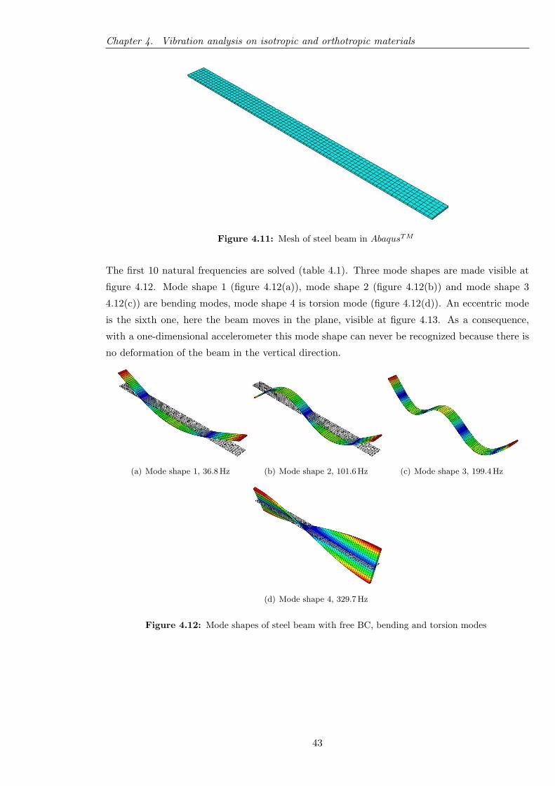
Chapter 4. Vibration analysis on isotropic and orthotropic materials
Figure 4.11: Mesh of steel beam in AbaqusTM
The first 10 natural frequencies are solved (table 4.1). Three mode shapes are made visible at
figure 4.12. Mode shape 1 (figure 4.12(a)), mode shape 2 (figure 4.12(b)) and mode shape 3
4.12(c)) are bending modes, mode shape 4 is torsion mode (figure 4.12(d)). An eccentric mode
is the sixth one, here the beam moves in the plane, visible at figure 4.13. As a consequence,
with a one-dimensional accelerometer this mode shape can never be recognized because there is
no deformation of the beam in the vertical direction.
(a) Mode shape 1, 36.8Hz (b) Mode shape 2, 101.6Hz (c) Mode shape 3, 199.4Hz
(d) Mode shape 4, 329.7Hz
Figure 4.12: Mode shapes of steel beam with free BC, bending and torsion modes
43

Chapter 4. Vibration analysis on isotropic and orthotropic materials
Figure 4.13: Mode shape of the steel beam with free BC - displacement in the plane of the beam
Experimental analysis
The steel beam is suspended by two soft elastic cords, the static deflection is 0.8 m. The lowest
rigid body mode has a frequency of fRBM,low = 12 ·π√g/δstatic = 1
2 ·π√
9.81/0.8 = 0.56 Hz [7].
In case of the length between the points of suspension is 550 mm, the next rigid body mode
(RBM) raises up to fRBM,high = 3.2 · fRBM,low = 1.8 Hz [7]. The calculated first elastic mode
of the beam is 36.8 Hz, so the ratio of elastic mode and rigid body mode is than 36.8/1.8 = 20
which is much higher than the desired value of 10 [29]. Of course, the higher the ratio, the less
the measured natural frequencies will be influenced by the elastic cords.
For the experimental test, the accelerometer is placed in a corner of the beam because for every
mode (except mode six) an acceleration is present on that point of the beam. The experimental
setup can be seen at figure 4.14.
Figure 4.14: Setup of experimental test for the steel beam with free BC
44
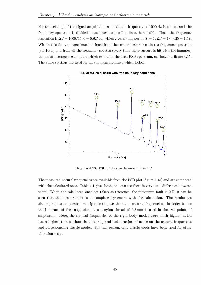
Chapter 4. Vibration analysis on isotropic and orthotropic materials
For the settings of the signal acquisition, a maximum frequency of 1000 Hz is chosen and the
frequency spectrum is divided in as much as possible lines, here 1600. Thus, the frequency
resolution is ∆f = 1000/1600 = 0.625 Hz which gives a time period T = 1/∆f = 1/0.625 = 1.6 s.
Within this time, the acceleration signal from the sensor is converted into a frequency spectrum
(via FFT) and from all the frequency spectra (every time the structure is hit with the hammer)
the linear average is calculated which results in the final PSD spectrum, as shown at figure 4.15.
The same settings are used for all the measurements which follow.
Figure 4.15: PSD of the steel beam with free BC
The measured natural frequencies are available from the PSD plot (figure 4.15) and are compared
with the calculated ones. Table 4.1 gives both, one can see there is very little difference between
them. When the calculated ones are taken as reference, the maximum fault is 2 %, it can be
seen that the measurement is in complete agreement with the calculation. The results are
also reproducable because multiple tests gave the same natural frequencies. In order to see
the influence of the suspension, also a nylon thread of 0.3 mm is used in the two points of
suspension. Here, the natural frequencies of the rigid body modes were much higher (nylon
has a higher stiffness than elastic cords) and had a major influence on the natural frequencies
and corresponding elastic modes. For this reason, only elastic cords have been used for other
vibration tests.
45
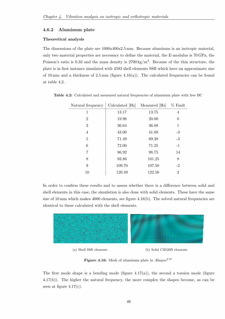
Chapter 4. Vibration analysis on isotropic and orthotropic materials
4.6.2 Aluminum plate
Theoretical analysis
The dimensions of the plate are 1000x400x2.5 mm. Because aluminum is an isotropic material,
only two material properties are necessary to define the material, the E-modulus is 70 GPa, the
Poisson’s ratio is 0.33 and the mass density is 2700 kg/m3. Because of the thin structure, the
plate is in first instance simulated with 4593 shell elements S8R which have an approximate size
of 10 mm and a thickness of 2.5 mm (figure 4.16(a)). The calculated frequencies can be found
at table 4.2.
Table 4.2: Calculated and measured natural frequencies of aluminum plate with free BC
Natural frequency Calculated [Hz] Measured [Hz] % Fault
1 13.17 13.75 4
2 19.98 20.00 0
3 36.64 36.88 1
4 43.00 41.88 -3
5 71.49 69.38 -3
6 72.00 71.25 -1
7 86.92 98.75 14
8 93.86 101.25 8
9 109.70 107.50 -2
10 120.49 122.50 2
In order to confirm these results and to assess whether there is a difference between solid and
shell elements in this case, the simulation is also done with solid elements. These have the same
size of 10 mm which makes 4000 elements, see figure 4.16(b). The solved natural frequencies are
identical to these calculated with the shell elements.
(a) Shell S8R elements (b) Solid C3D20R elements
Figure 4.16: Mesh of aluminum plate in AbaqusTM
The first mode shape is a bending mode (figure 4.17(a)), the second a torsion mode (figure
4.17(b)). The higher the natural frequency, the more complex the shapes become, as can be
seen at figure 4.17(c).
46

Chapter 4. Vibration analysis on isotropic and orthotropic materials
(a) Mode shape 1, 13.17Hz (b) Mode shape 2, 19.98Hz (c) Mode shape 10, 120.49Hz
Figure 4.17: Mode shapes of aluminium plate in a free condition
Experimental analysis
The test setup for the aluminum plate is analogue to that of the steel beam. Again, free BC are
used and the accelerometer is placed at the plate, as can be seen at figure 4.18.
Figure 4.18: Setup of experimental test for the aluminum plate as a free body
The vibration test has been done for several times on this plate, every time the same natural
frequencies were visible in the PSD plot, shown at figure 4.20. When making the comparison
with the calculated values, the results are quit good, the maximum error here is 14 %. Table
4.2 shows the measured and calculated natural frequencies with the procentual error. When
having a closer look at mode shape 7 (with the procentual error of 14 %), from the AbaqusTM
simulation, a sort of bending mode is identified (figure 4.19). This kind of mode shape leans
close to the static deformation of the plate (due to its own weight) when suspended on four
points at the corners, which is the case for this setup (figure 4.18). Because of the similarity
between the simulated mode shape and the static deformation of the plate, it is reasonable that
this is the reason for the high procentual error. So, the static deformation shape influences the
natural frequency which corresponds with the identical simulated mode shape.
47
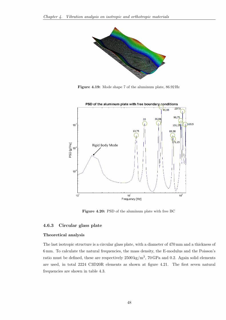
Chapter 4. Vibration analysis on isotropic and orthotropic materials
Figure 4.19: Mode shape 7 of the aluminum plate, 86.92 Hz
Figure 4.20: PSD of the aluminum plate with free BC
4.6.3 Circular glass plate
Theoretical analysis
The last isotropic structure is a circular glass plate, with a diameter of 470 mm and a thickness of
6 mm. To calculate the natural frequencies, the mass density, the E-modulus and the Poisson’s
ratio must be defined, these are respectively 2500 kg/m3, 70 GPa and 0.2. Again solid elements
are used, in total 2224 C3D20R elements as shown at figure 4.21. The first seven natural
frequencies are shown in table 4.3.
48
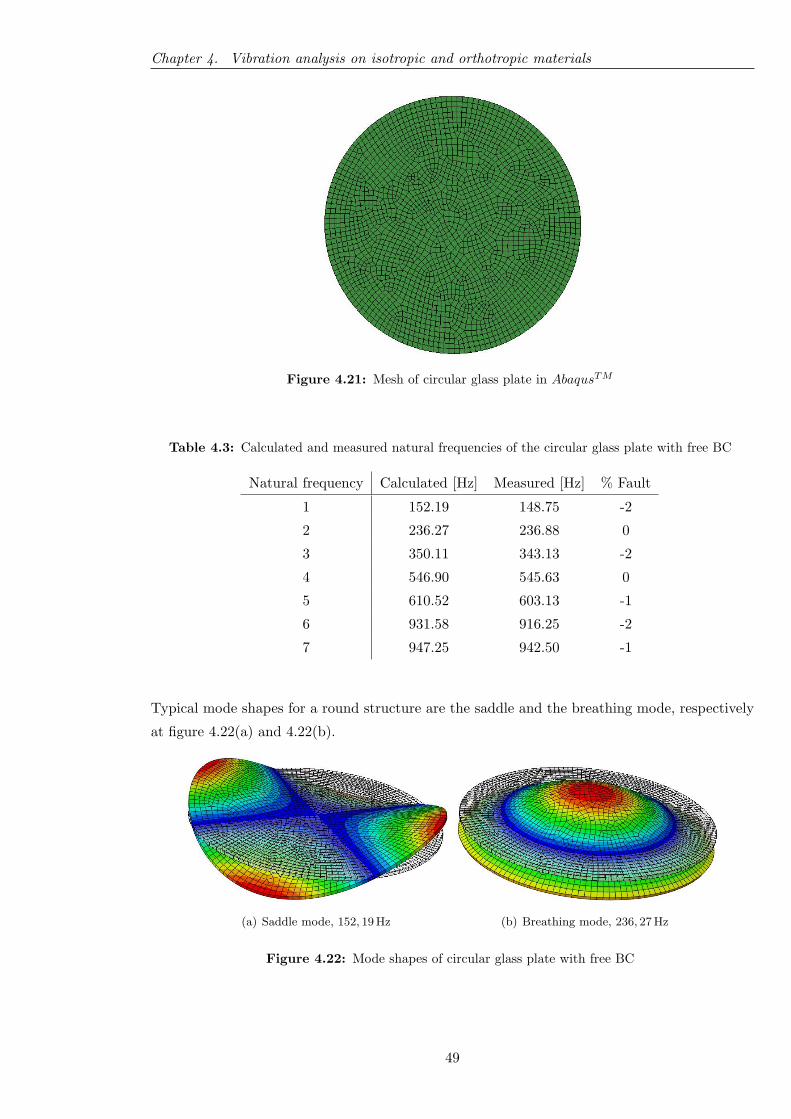
Chapter 4. Vibration analysis on isotropic and orthotropic materials
Figure 4.21: Mesh of circular glass plate in AbaqusTM
Table 4.3: Calculated and measured natural frequencies of the circular glass plate with free BC
Natural frequency Calculated [Hz] Measured [Hz] % Fault
1 152.19 148.75 -2
2 236.27 236.88 0
3 350.11 343.13 -2
4 546.90 545.63 0
5 610.52 603.13 -1
6 931.58 916.25 -2
7 947.25 942.50 -1
Typical mode shapes for a round structure are the saddle and the breathing mode, respectively
at figure 4.22(a) and 4.22(b).
(a) Saddle mode, 152, 19Hz (b) Breathing mode, 236, 27Hz
Figure 4.22: Mode shapes of circular glass plate with free BC
49
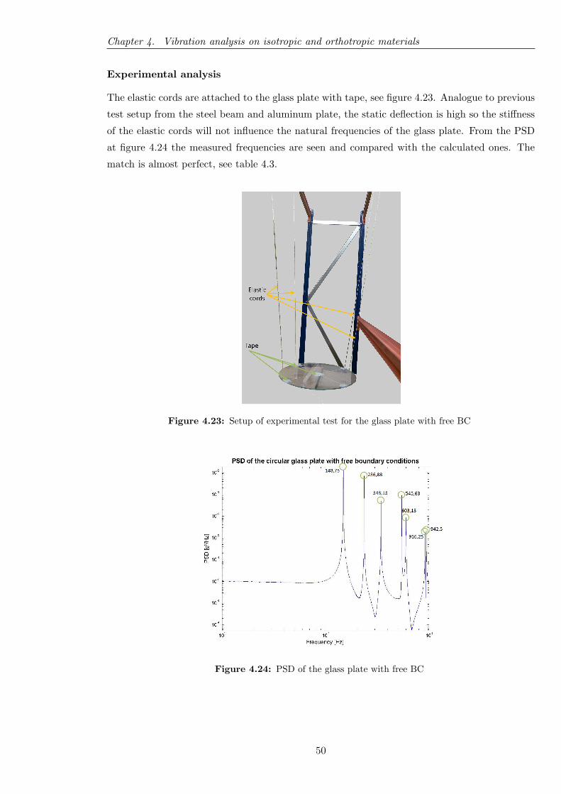
Chapter 4. Vibration analysis on isotropic and orthotropic materials
Experimental analysis
The elastic cords are attached to the glass plate with tape, see figure 4.23. Analogue to previous
test setup from the steel beam and aluminum plate, the static deflection is high so the stiffness
of the elastic cords will not influence the natural frequencies of the glass plate. From the PSD
at figure 4.24 the measured frequencies are seen and compared with the calculated ones. The
match is almost perfect, see table 4.3.
Figure 4.23: Setup of experimental test for the glass plate with free BC
Figure 4.24: PSD of the glass plate with free BC
50

Chapter 4. Vibration analysis on isotropic and orthotropic materials
4.7 Vibration testing on orthotropic materials
Since the purpose of this master thesis is to assess composite bicycle frames, some test are
performed on composite structures with a simple geometry. The first one is a Uni-Directional
(UD)-Carbon composite, the second one is a C-PPS 5 harness satin weave carbon composite.
C-PPS stands for Carbon-Polyphenylene Sulfide, the resin (PPS) is a high-performance
thermoplastic.
4.7.1 UD-Carbon composite
Theoretical analysis
The dimensions of this composite plate are 246x170x2.2 mm, the mass density is 1733 kg/m3.
Because of the orthotropic character of the composite, nine independent property values must
be defined which are listed on table 4.4. From a tensile test, only E11, E22, ν12 and G12 can be
determined. The other ones are an approach because these cannot be measured. A method to
find these out of plane properties is found at [30].
Because of the low weight (160 g) of the structure, the mass of the accelerometer is taken into
account for the AbaqusTM calculations. This is implemented as a point mass of 5 g. With a
size of 5 mm for the solid C3D20R elements, 1666 elements are present. The fibre direction is
the same for all the layers (UD), so the plate can be simulated as one solid structure but the
material directions must be defined in AbaqusTM . These directions are shown on the setup
condition for the measurements at figure 4.25.
Table 4.4: Material properties of the UD-Carbon composite
E11 [GPa] E22 [GPa] E33 [GPa] ν12 ν13 ν23 G12 [MPa] G13 [MPa] G23 [MPa]
171.24 7.966 7.966 0.3 0.3 0.3 5191.18 5191.18 5191.18
Experimental analysis
The plate is suspended with four elastic cords and the accelerometer is put into a corner to make
sure that every mode shape is registered. For every mode shape, there is always deforming of
the plate at the corners, as was seen from the AbaqusTM simulation. The first mode shape is a
torsion mode and the second is a bending mode, the mode shapes are analogue to these of the
aluminum plate at figure 4.17(b) respectively figure 4.17(a).
51
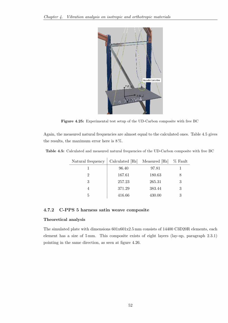
Chapter 4. Vibration analysis on isotropic and orthotropic materials
Figure 4.25: Experimental test setup of the UD-Carbon composite with free BC
Again, the measured natural frequencies are almost equal to the calculated ones. Table 4.5 gives
the results, the maximum error here is 8 %.
Table 4.5: Calculated and measured natural frequencies of the UD-Carbon composite with free BC
Natural frequency Calculated [Hz] Measured [Hz] % Fault
1 96.40 97.81 1
2 167.61 180.63 8
3 257.23 265.31 3
4 371.29 383.44 3
5 416.66 430.00 3
4.7.2 C-PPS 5 harness satin weave composite
Theoretical analysis
The simulated plate with dimensions 601x601x2.5 mm consists of 14400 C3D20R elements, each
element has a size of 5 mm. This composite exists of eight layers (lay-up, paragraph 2.3.1)
pointing in the same direction, as seen at figure 4.26.
52

Chapter 4. Vibration analysis on isotropic and orthotropic materials
Figure 4.26: Ply stack of the C-PPS 5 harness satin weave composite
Like the previous composite, nine mechanical property values must be defined, these are
enumerated in table 4.6. Only E11, E22, G12 and ν12 are found by experiments, the others must
be calculated.
Table 4.6: Material properties of the C-PPS 5 harness satin weave composite
E11 [GPa] E22 [GPa] E33 [GPa] ν12 ν13 ν23 G12 [MPa] G13 [MPa] G23 [MPa]
57.240 57.240 9.700 0.04 0.38 0.38 4142 2904 2902
The natural frequencies and mode shapes are solved again, the frequencies are listed on table
4.7. The first mode shape is a torsion mode and is presented at figure 4.27.
Figure 4.27: First mode of the C-PPS 5 harness satin weave composite
Experimental analysis
The current test setup is identical to the test setup seen at figure 4.25. Surprisingly, the first
measured natural frequency is not the simulated one of 11.7 Hz but 18.4 Hz as seen at table 4.7
53
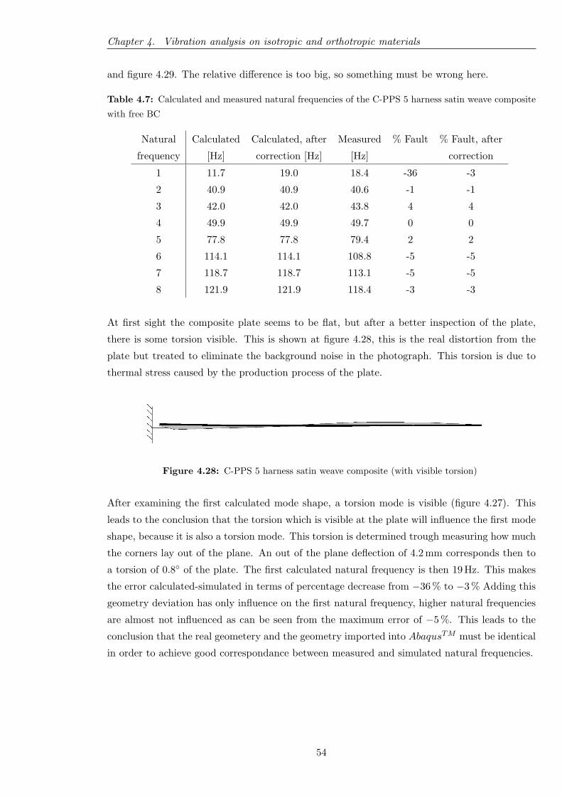
Chapter 4. Vibration analysis on isotropic and orthotropic materials
and figure 4.29. The relative difference is too big, so something must be wrong here.
Table 4.7: Calculated and measured natural frequencies of the C-PPS 5 harness satin weave composite
with free BC
Natural Calculated Calculated, after Measured % Fault % Fault, after
frequency [Hz] correction [Hz] [Hz] correction
1 11.7 19.0 18.4 -36 -3
2 40.9 40.9 40.6 -1 -1
3 42.0 42.0 43.8 4 4
4 49.9 49.9 49.7 0 0
5 77.8 77.8 79.4 2 2
6 114.1 114.1 108.8 -5 -5
7 118.7 118.7 113.1 -5 -5
8 121.9 121.9 118.4 -3 -3
At first sight the composite plate seems to be flat, but after a better inspection of the plate,
there is some torsion visible. This is shown at figure 4.28, this is the real distortion from the
plate but treated to eliminate the background noise in the photograph. This torsion is due to
thermal stress caused by the production process of the plate.
Figure 4.28: C-PPS 5 harness satin weave composite (with visible torsion)
After examining the first calculated mode shape, a torsion mode is visible (figure 4.27). This
leads to the conclusion that the torsion which is visible at the plate will influence the first mode
shape, because it is also a torsion mode. This torsion is determined trough measuring how much
the corners lay out of the plane. An out of the plane deflection of 4.2 mm corresponds then to
a torsion of 0.8◦ of the plate. The first calculated natural frequency is then 19 Hz. This makes
the error calculated-simulated in terms of percentage decrease from −36 % to −3 % Adding this
geometry deviation has only influence on the first natural frequency, higher natural frequencies
are almost not influenced as can be seen from the maximum error of −5 %. This leads to the
conclusion that the real geometery and the geometry imported into AbaqusTM must be identical
in order to achieve good correspondance between measured and simulated natural frequencies.
54
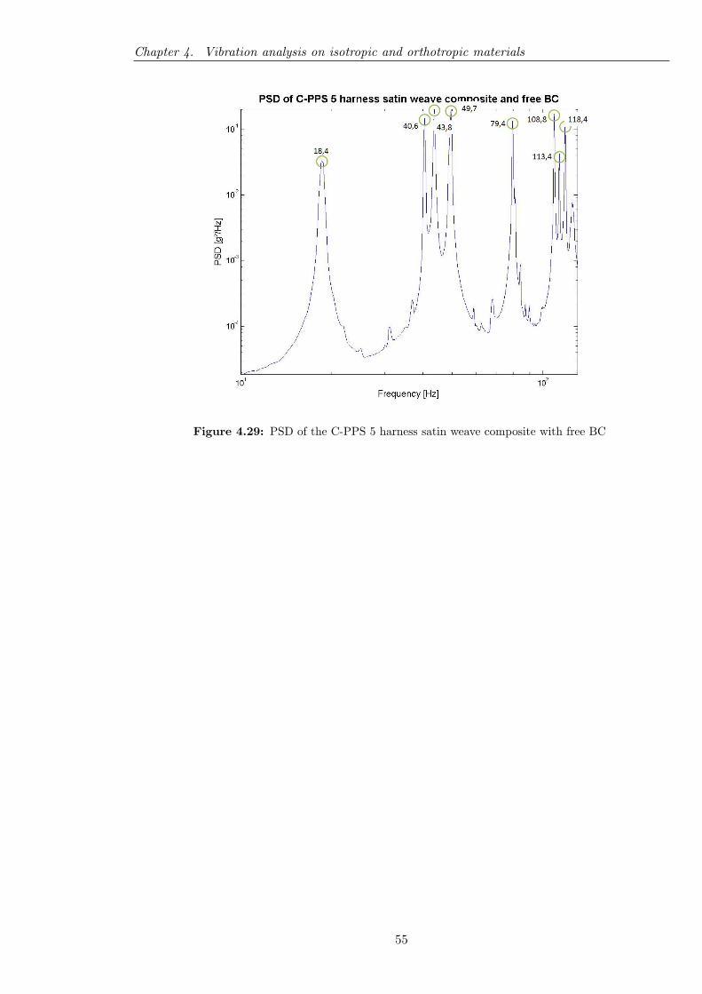
Chapter 4. Vibration analysis on isotropic and orthotropic materials
Figure 4.29: PSD of the C-PPS 5 harness satin weave composite with free BC
55

Chapter 5
Dynamic behaviour of flax/carbon
reinforced composite bicycle frames
5.1 Introduction
The main goal of this chapter is to assess the dynamic behaviour of the MF1 (Museeuw Flax
1) and MF5 flax-carbon reinforced composite bicycle frames. The MF1 has a flax-carbon ratio
of 50-50, this means that the quantity flax and carbon is equal distributed. In case of the MF5
frame, 80 % flax is present in the frame. By means of experimental modal analysis the natural
frequency and the mode shape of both frames will be estimated. Also a numerical computer
model of the MF1 frame has been built.
(a) MF1 bicycle (b) MF5 bicycle
Figure 5.1: MF1 and MF5 bicycles
5.2 Numerical model of the MF1 frame
The goal of making a numerical computer model of a structure is not only to correlate the
simulated results with the experimental results, but it also helps to understand how a complex
structure behaves when a load or vibration is applied to it. In case of the bicycle frame, the
visualization of the mode shapes (when calculating the natural frequencies with AbaqusTM )
makes it possible to see which parts of the frame will deform the most when a time varying force
56
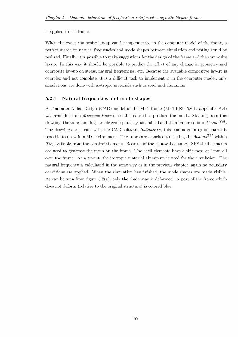
Chapter 5. Dynamic behaviour of flax/carbon reinforced composite bicycle frames
is applied to the frame.
When the exact composite lay-up can be implemented in the computer model of the frame, a
perfect match on natural frequencies and mode shapes between simulation and testing could be
realized. Finally, it is possible to make suggestions for the design of the frame and the composite
layup. In this way it should be possible to predict the effect of any change in geometry and
composite lay-up on stress, natural frequencies, etc. Because the available compositye lay-up is
complex and not complete, it is a difficult task to implement it in the computer model, only
simulations are done with isotropic materials such as steel and aluminum.
5.2.1 Natural frequencies and mode shapes
A Computer-Aided Design (CAD) model of the MF1 frame (MF1-R839-580L, appendix A.4)
was available from Museeuw Bikes since this is used to produce the molds. Starting from this
drawing, the tubes and lugs are drawn separately, assembled and than imported into AbaqusTM .
The drawings are made with the CAD-software Solidworks, this computer program makes it
possible to draw in a 3D environment. The tubes are attached to the lugs in AbaqusTM with a
Tie, available from the constraints menu. Because of the thin-walled tubes, SR8 shell elements
are used to generate the mesh on the frame. The shell elements have a thickness of 2 mm all
over the frame. As a tryout, the isotropic material aluminum is used for the simulation. The
natural frequency is calculated in the same way as in the previous chapter, again no boundary
conditions are applied. When the simulation has finished, the mode shapes are made visible.
As can be seen from figure 5.2(a), only the chain stay is deformed. A part of the frame which
does not deform (relative to the original structure) is colored blue.
57
Chapter 5. Dynamic behaviour of flax/carbon reinforced composite bicycle frames
(a) Mode shape 1, 135Hz (b) Mode shape 2, 144Hz
(c) Mode shape 3, 329Hz (d) Mode shape 4, 366Hz
Figure 5.2: Mode shapes from the MF1 frame - 2 mm thick aluminum shell elements
5.2.2 Influence of tube thickness and frame material
In order to see what the influence is on the thickness of the tubes and lugs, the thickness has
decreased from 2 mm up to 1 mm. The mesh and material has stayed the same as the previous
simulation. After simulation, it is seen that the mode shapes are exactly the same but the natural
frequencies are shifted down. When the simulation is done with steel instead of aluminum, the
natural frequencies shift up a little bit (circa 1 %).
5.3 Single Degree Of Freedom: the forced vibration
As mentioned already at paragraph 4.2, experimental modal analysis (EMA) requires a force
which interacts with the structure (here: the bicycle frame). This means that a forced vibration
takes place. As an introduction to more complex analysis about EMA, first the theory about
the forced vibration is explained for a Single Degree Of Freedom (SDOF) structure.
58

Chapter 5. Dynamic behaviour of flax/carbon reinforced composite bicycle frames
A structure which has only one degree of freedom is called a SDOF structure. The number of
DOF’s is specified by the number of masses which are coupled with each other by a stiffness k
and a damper c. A SDOF structure has only one natural frequency, one mode shape and one
damping factor. A schematic representation of such a system is found at figure 5.3. Because
any structure like a beam, a plate, etc. exists of an infinite number of infinitesimal small
mass-damper-spring systems, each structure has an infinite number of mode shapes and natural
frequencies. Such a structure is a Multi Degree Of Freedom (MDOF) structure. The reader
may already have noticed this at the previous chapter, different peaks (cf. natural frequencies)
are seen at the PSD plots.
The study of the dynamic behaviour requires the presence of a force, this force is attached to
the structure. The SDOF system is evaluated when a time varying force f(t) = F cos(ωt) is
imposed to it.
Figure 5.3: Forced vibration system
The system is set free from its environment by applying forces which work onto the system, this
is shown at figure 5.4.
Figure 5.4: Setting free the SDOF forced vibration system
From the third law of Newton follows:∑F = m · x:
mg + f(t)− k(x+ δstat)− cx = mx
mx+ cx+ kx = f(t)
md2x
dt2+ c
dx
dt+ kx = f(t) (5.1)
59
Chapter 5. Dynamic behaviour of flax/carbon reinforced composite bicycle frames
The differential equation (5.1) has two solutions. The first one is the transitional regime, which
is found by setting f(t) = 0.
x1(t) = Xde−ζω0t cos (ωdt− φd)
The second solution is the steady state state regime:
x2(t) = X cos (ωt− φ)
The total displacement x(t) is found using superposition: x(t) = x1(t) + x2(t). Finally, after
the menopausal symptom has died out, the system vibrates with the same frequency as the
harmonic force f(t) but there is a phase shift φ between force f(t) and displacement x(t). As
found at [7], formulas for amplitude X and phase φ are written as:
φ = arctan(
2βζ1− β2
)(5.2)
X
Xstat=
1√(2βζ)2 + (1− β2)2
(5.3)
With: β = ωω0
Tuning factorX
XstatResonate factor: ratio from dynamic and static deformation
Xstat = FK Static deformation of the system when the excitation force F applies
to it.The frequency for which X/Xstat reaches its maximum is the resonate frequency
ωr = ω0
√1− 2ζ2. For light damped structures (ζ < 1%) X/Xstat reaches than its
maximum value of 12ζ .
Figures 5.5(a) and 5.5(b) depict respectively equation (5.2) and (5.3). At low frequency (β <<
1), the response x(t) is dominated by the spring and is in phase with the excitation f(t).
As frequency increases (β ↗), the inertial force of the mass has an increasing influence. At
undamped natural frequency ω0 (β = 1) the mass and spring terms cancel each other out,
the response is controlled only by the damping term, and compliance (=displacement/force)
becomes high. If the damping term was, in fact, zero the compliance would be infinite. At ω0,
the response lags the excitation by 90◦. At frequencies greater than ω0 (β >> 1), the mass term
takes control, the system begins to behave simply as a mass, the compliance decreases and the
response lags the excitation by 180◦.
60
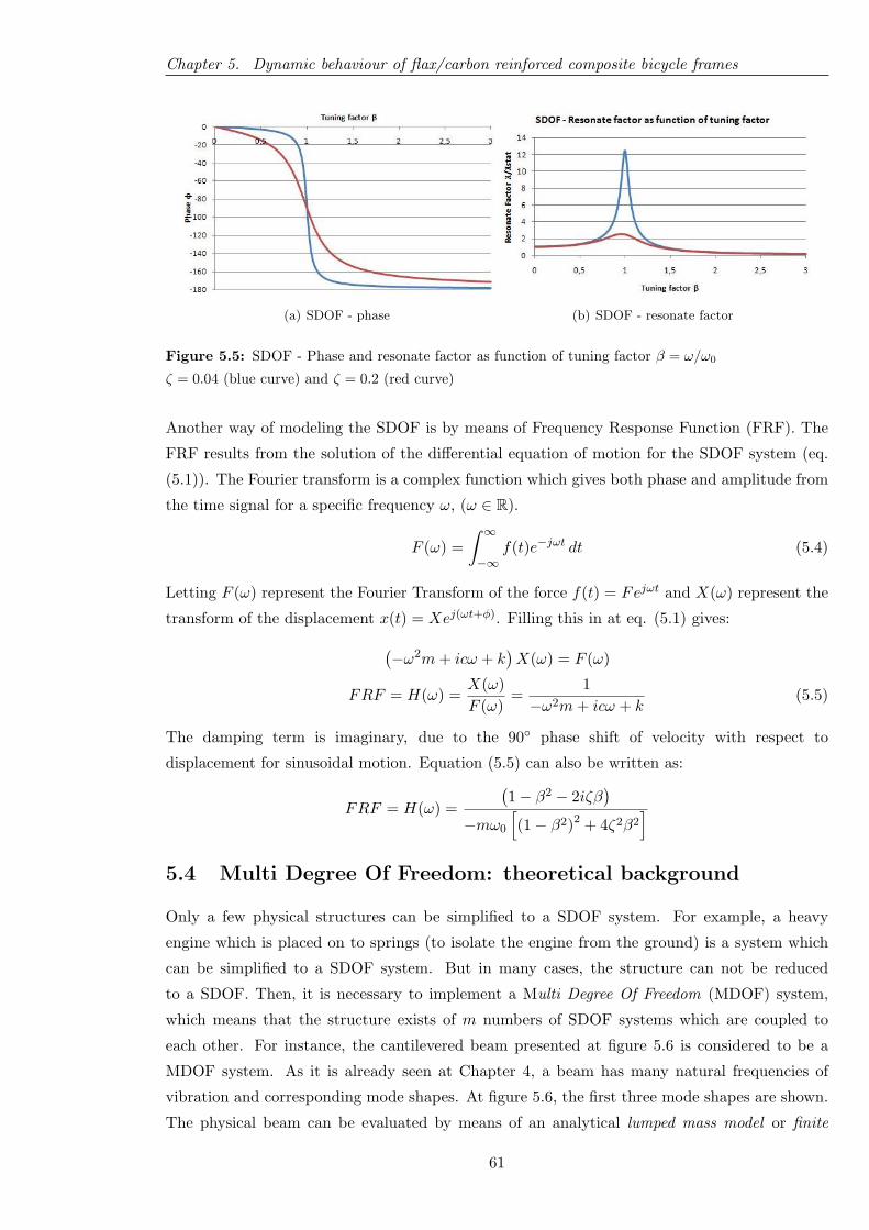
Chapter 5. Dynamic behaviour of flax/carbon reinforced composite bicycle frames
(a) SDOF - phase (b) SDOF - resonate factor
Figure 5.5: SDOF - Phase and resonate factor as function of tuning factor β = ω/ω0
ζ = 0.04 (blue curve) and ζ = 0.2 (red curve)
Another way of modeling the SDOF is by means of Frequency Response Function (FRF). The
FRF results from the solution of the differential equation of motion for the SDOF system (eq.
(5.1)). The Fourier transform is a complex function which gives both phase and amplitude from
the time signal for a specific frequency ω, (ω ∈ R).
F (ω) =∫ ∞−∞
f(t)e−jωt dt (5.4)
Letting F (ω) represent the Fourier Transform of the force f(t) = Fejωt and X(ω) represent the
transform of the displacement x(t) = Xej(ωt+φ). Filling this in at eq. (5.1) gives:(−ω2m+ icω + k
)X(ω) = F (ω)
FRF = H(ω) =X(ω)F (ω)
=1
−ω2m+ icω + k(5.5)
The damping term is imaginary, due to the 90◦ phase shift of velocity with respect to
displacement for sinusoidal motion. Equation (5.5) can also be written as:
FRF = H(ω) =
(1− β2 − 2iζβ
)−mω0
[(1− β2)2 + 4ζ2β2
]5.4 Multi Degree Of Freedom: theoretical background
Only a few physical structures can be simplified to a SDOF system. For example, a heavy
engine which is placed on to springs (to isolate the engine from the ground) is a system which
can be simplified to a SDOF system. But in many cases, the structure can not be reduced
to a SDOF. Then, it is necessary to implement a Multi Degree Of Freedom (MDOF) system,
which means that the structure exists of m numbers of SDOF systems which are coupled to
each other. For instance, the cantilevered beam presented at figure 5.6 is considered to be a
MDOF system. As it is already seen at Chapter 4, a beam has many natural frequencies of
vibration and corresponding mode shapes. At figure 5.6, the first three mode shapes are shown.
The physical beam can be evaluated by means of an analytical lumped mass model or finite
61
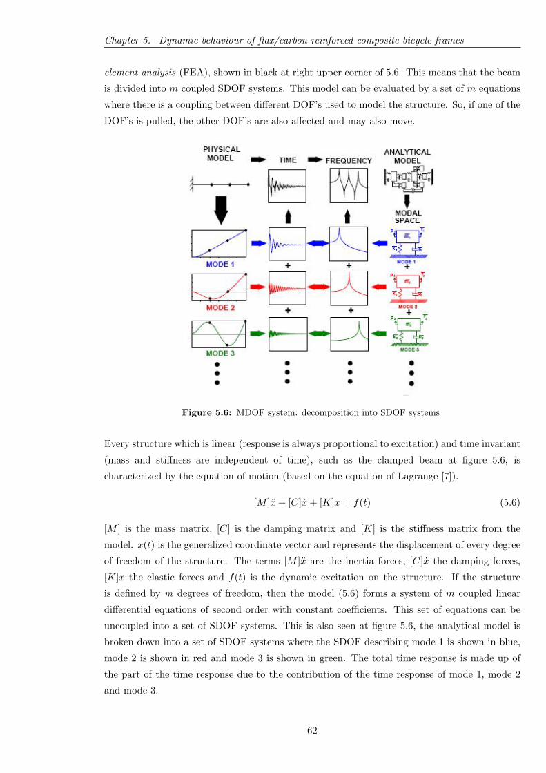
Chapter 5. Dynamic behaviour of flax/carbon reinforced composite bicycle frames
element analysis (FEA), shown in black at right upper corner of 5.6. This means that the beam
is divided into m coupled SDOF systems. This model can be evaluated by a set of m equations
where there is a coupling between different DOF’s used to model the structure. So, if one of the
DOF’s is pulled, the other DOF’s are also affected and may also move.
Figure 5.6: MDOF system: decomposition into SDOF systems
Every structure which is linear (response is always proportional to excitation) and time invariant
(mass and stiffness are independent of time), such as the clamped beam at figure 5.6, is
characterized by the equation of motion (based on the equation of Lagrange [7]).
[M ]x+ [C]x+ [K]x = f(t) (5.6)
[M ] is the mass matrix, [C] is the damping matrix and [K] is the stiffness matrix from the
model. x(t) is the generalized coordinate vector and represents the displacement of every degree
of freedom of the structure. The terms [M ]x are the inertia forces, [C]x the damping forces,
[K]x the elastic forces and f(t) is the dynamic excitation on the structure. If the structure
is defined by m degrees of freedom, then the model (5.6) forms a system of m coupled linear
differential equations of second order with constant coefficients. This set of equations can be
uncoupled into a set of SDOF systems. This is also seen at figure 5.6, the analytical model is
broken down into a set of SDOF systems where the SDOF describing mode 1 is shown in blue,
mode 2 is shown in red and mode 3 is shown in green. The total time response is made up of
the part of the time response due to the contribution of the time response of mode 1, mode 2
and mode 3.
62
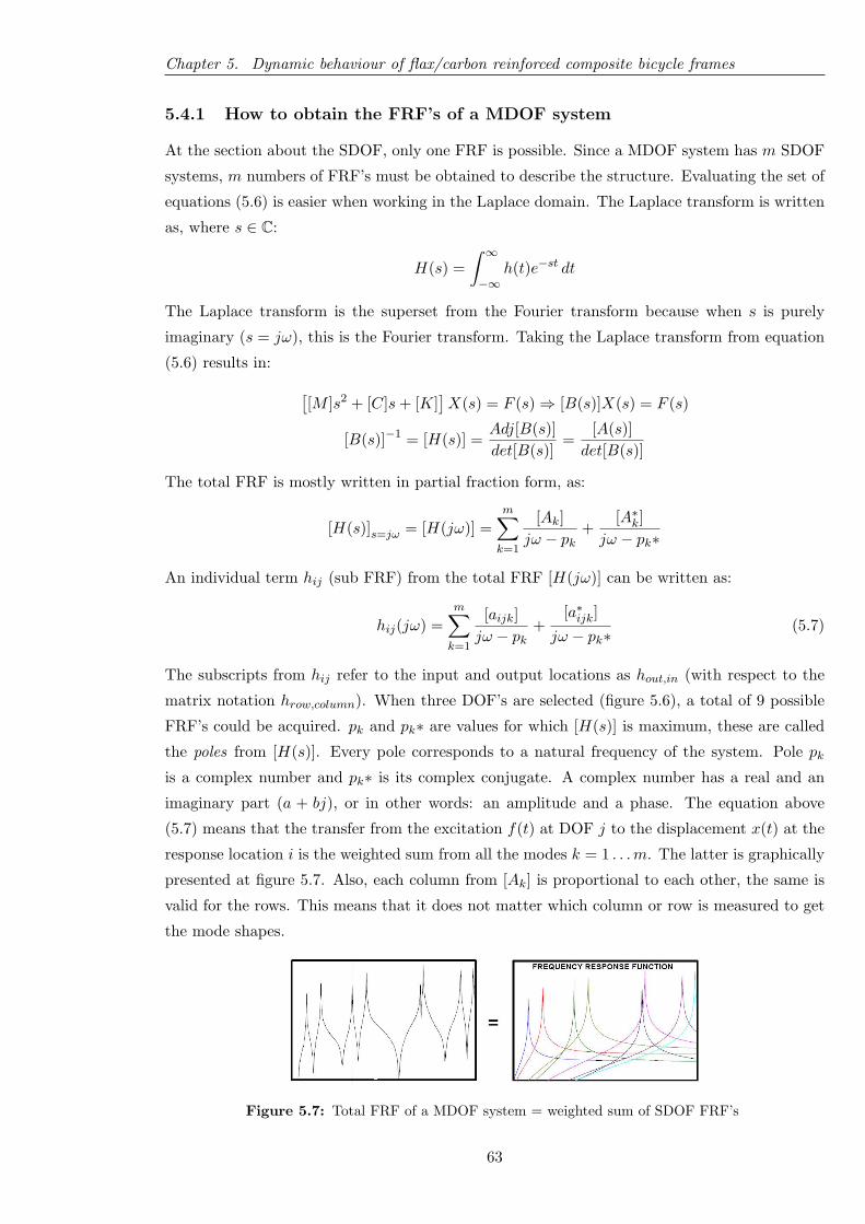
Chapter 5. Dynamic behaviour of flax/carbon reinforced composite bicycle frames
5.4.1 How to obtain the FRF’s of a MDOF system
At the section about the SDOF, only one FRF is possible. Since a MDOF system has m SDOF
systems, m numbers of FRF’s must be obtained to describe the structure. Evaluating the set of
equations (5.6) is easier when working in the Laplace domain. The Laplace transform is written
as, where s ∈ C:
H(s) =∫ ∞−∞
h(t)e−st dt
The Laplace transform is the superset from the Fourier transform because when s is purely
imaginary (s = jω), this is the Fourier transform. Taking the Laplace transform from equation
(5.6) results in: [[M ]s2 + [C]s+ [K]
]X(s) = F (s)⇒ [B(s)]X(s) = F (s)
[B(s)]−1 = [H(s)] =Adj[B(s)]det[B(s)]
=[A(s)]
det[B(s)]
The total FRF is mostly written in partial fraction form, as:
[H(s)]s=jω = [H(jω)] =m∑k=1
[Ak]jω − pk
+[A∗k]
jω − pk∗
An individual term hij (sub FRF) from the total FRF [H(jω)] can be written as:
hij(jω) =m∑k=1
[aijk]jω − pk
+[a∗ijk]
jω − pk∗(5.7)
The subscripts from hij refer to the input and output locations as hout,in (with respect to the
matrix notation hrow,column). When three DOF’s are selected (figure 5.6), a total of 9 possible
FRF’s could be acquired. pk and pk∗ are values for which [H(s)] is maximum, these are called
the poles from [H(s)]. Every pole corresponds to a natural frequency of the system. Pole pkis a complex number and pk∗ is its complex conjugate. A complex number has a real and an
imaginary part (a + bj), or in other words: an amplitude and a phase. The equation above
(5.7) means that the transfer from the excitation f(t) at DOF j to the displacement x(t) at the
response location i is the weighted sum from all the modes k = 1 . . .m. The latter is graphically
presented at figure 5.7. Also, each column from [Ak] is proportional to each other, the same is
valid for the rows. This means that it does not matter which column or row is measured to get
the mode shapes.
Figure 5.7: Total FRF of a MDOF system = weighted sum of SDOF FRF’s
63
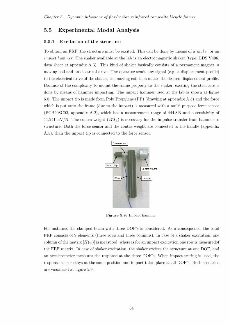
Chapter 5. Dynamic behaviour of flax/carbon reinforced composite bicycle frames
5.5 Experimental Modal Analysis
5.5.1 Excitation of the structure
To obtain an FRF, the structure must be excited. This can be done by means of a shaker or an
impact hammer. The shaker available at the lab is an electromagnetic shaker (type: LDS V406,
data sheet at appendix A.3). This kind of shaker basically consists of a permanent magnet, a
moving coil and an electrical drive. The operator sends any signal (e.g. a displacement profile)
to the electrical drive of the shaker, the moving coil then makes the desired displacement profile.
Because of the complexity to mount the frame properly to the shaker, exciting the structure is
done by means of hammer impacting. The impact hammer used at the lab is shown at figure
5.8. The impact tip is made from Poly Propylene (PP) (drawing at appendix A.5) and the force
which is put onto the frame (due to the impact) is measured with a multi purpose force sensor
(PCB208C02, appendix A.2), which has a measurement range of 444.8 N and a sensitivity of
11.241 mV/N. The contra weight (270 g) is necessary for the impulse transfer from hammer to
structure. Both the force sensor and the contra weight are connected to the handle (appendix
A.5), than the impact tip is connected to the force sensor.
Figure 5.8: Impact hammer
For instance, the clamped beam with three DOF’s is considered. As a consequence, the total
FRF consists of 9 elements (three rows and three columns). In case of a shaker excitation, one
column of the matrix [H(ω)] is measured, whereas for an impact excitation one row is measuredof
the FRF matrix. In case of shaker excitation, the shaker excites the structure at one DOF, and
an accelerometer measures the response at the three DOF’s. When impact testing is used, the
response sensor stays at the same position and impact takes place at all DOF’s. Both scenarios
are visualized at figure 5.9.
64
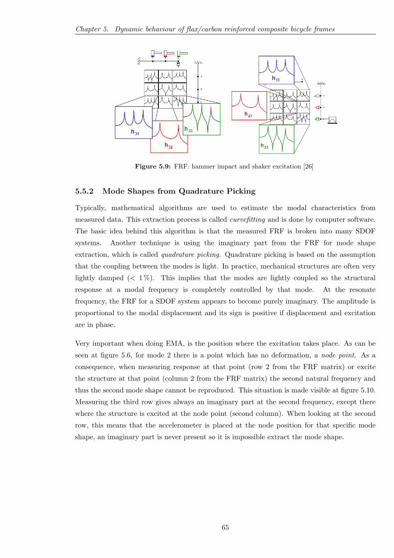
Chapter 5. Dynamic behaviour of flax/carbon reinforced composite bicycle frames
Figure 5.9: FRF: hammer impact and shaker excitation [26]
5.5.2 Mode Shapes from Quadrature Picking
Typically, mathematical algorithms are used to estimate the modal characteristics from
measured data. This extraction process is called curvefitting and is done by computer software.
The basic idea behind this algorithm is that the measured FRF is broken into many SDOF
systems. Another technique is using the imaginary part from the FRF for mode shape
extraction, which is called quadrature picking. Quadrature picking is based on the assumption
that the coupling between the modes is light. In practice, mechanical structures are often very
lightly damped (< 1 %). This implies that the modes are lightly coupled so the structural
response at a modal frequency is completely controlled by that mode. At the resonate
frequency, the FRF for a SDOF system appears to become purely imaginary. The amplitude is
proportional to the modal displacement and its sign is positive if displacement and excitation
are in phase.
Very important when doing EMA, is the position where the excitation takes place. As can be
seen at figure 5.6, for mode 2 there is a point which has no deformation, a node point. As a
consequence, when measuring response at that point (row 2 from the FRF matrix) or excite
the structure at that point (column 2 from the FRF matrix) the second natural frequency and
thus the second mode shape cannot be reproduced. This situation is made visible at figure 5.10.
Measuring the third row gives always an imaginary part at the second frequency, except there
where the structure is excited at the node point (second column). When looking at the second
row, this means that the accelerometer is placed at the node position for that specific mode
shape, an imaginary part is never present so it is impossible extract the mode shape.
65
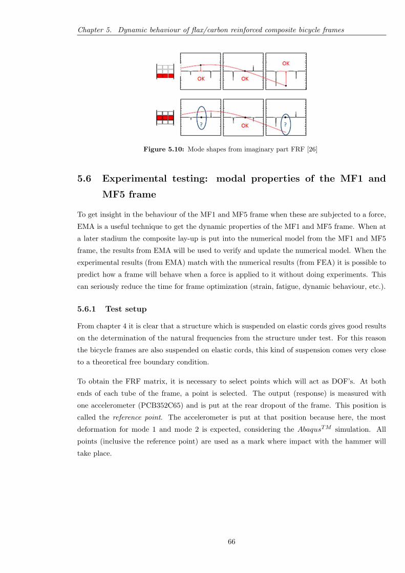
Chapter 5. Dynamic behaviour of flax/carbon reinforced composite bicycle frames
Figure 5.10: Mode shapes from imaginary part FRF [26]
5.6 Experimental testing: modal properties of the MF1 and
MF5 frame
To get insight in the behaviour of the MF1 and MF5 frame when these are subjected to a force,
EMA is a useful technique to get the dynamic properties of the MF1 and MF5 frame. When at
a later stadium the composite lay-up is put into the numerical model from the MF1 and MF5
frame, the results from EMA will be used to verify and update the numerical model. When the
experimental results (from EMA) match with the numerical results (from FEA) it is possible to
predict how a frame will behave when a force is applied to it without doing experiments. This
can seriously reduce the time for frame optimization (strain, fatigue, dynamic behaviour, etc.).
5.6.1 Test setup
From chapter 4 it is clear that a structure which is suspended on elastic cords gives good results
on the determination of the natural frequencies from the structure under test. For this reason
the bicycle frames are also suspended on elastic cords, this kind of suspension comes very close
to a theoretical free boundary condition.
To obtain the FRF matrix, it is necessary to select points which will act as DOF’s. At both
ends of each tube of the frame, a point is selected. The output (response) is measured with
one accelerometer (PCB352C65) and is put at the rear dropout of the frame. This position is
called the reference point. The accelerometer is put at that position because here, the most
deformation for mode 1 and mode 2 is expected, considering the AbaqusTM simulation. All
points (inclusive the reference point) are used as a mark where impact with the hammer will
take place.
66
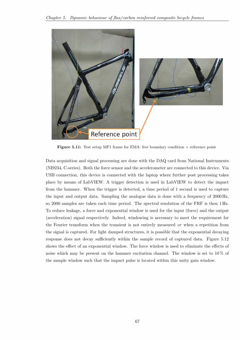
Chapter 5. Dynamic behaviour of flax/carbon reinforced composite bicycle frames
Figure 5.11: Test setup MF1 frame for EMA: free boundary condition + reference point
Data acquisition and signal processing are done with the DAQ card from National Instruments
(NI9234, C-series). Both the force sensor and the accelerometer are connected to this device. Via
USB connection, this device is connected with the laptop where further post processing takes
place by means of LabVIEW. A trigger detection is used in LabVIEW to detect the impact
from the hammer. When the trigger is detected, a time period of 1 second is used to capture
the input and output data. Sampling the analogue data is done with a frequency of 2000 Hz,
so 2000 samples are taken each time period. The spectral resolution of the FRF is then 1 Hz.
To reduce leakage, a force and exponential window is used for the input (force) and the output
(acceleration) signal respectively. Indeed, windowing is necessary to meet the requirement for
the Fourier transform when the transient is not entirely measured or when a repetition from
the signal is captured. For light damped structures, it is possible that the exponential decaying
response does not decay sufficiently within the sample record of captured data. Figure 5.12
shows the effect of an exponential window. The force window is used to eliminate the effects of
noise which may be present on the hammer excitation channel. The window is set to 10 % of
the sample window such that the impact pulse is located within this unity gain window.
67
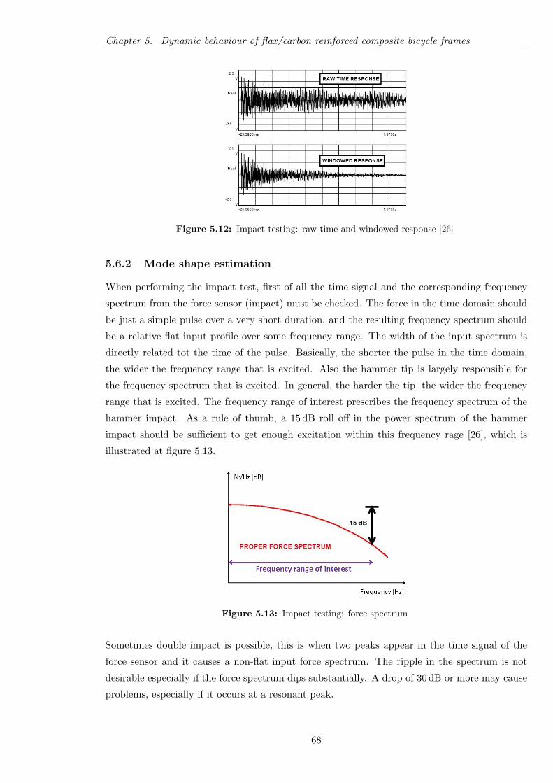
Chapter 5. Dynamic behaviour of flax/carbon reinforced composite bicycle frames
Figure 5.12: Impact testing: raw time and windowed response [26]
5.6.2 Mode shape estimation
When performing the impact test, first of all the time signal and the corresponding frequency
spectrum from the force sensor (impact) must be checked. The force in the time domain should
be just a simple pulse over a very short duration, and the resulting frequency spectrum should
be a relative flat input profile over some frequency range. The width of the input spectrum is
directly related tot the time of the pulse. Basically, the shorter the pulse in the time domain,
the wider the frequency range that is excited. Also the hammer tip is largely responsible for
the frequency spectrum that is excited. In general, the harder the tip, the wider the frequency
range that is excited. The frequency range of interest prescribes the frequency spectrum of the
hammer impact. As a rule of thumb, a 15 dB roll off in the power spectrum of the hammer
impact should be sufficient to get enough excitation within this frequency rage [26], which is
illustrated at figure 5.13.
Figure 5.13: Impact testing: force spectrum
Sometimes double impact is possible, this is when two peaks appear in the time signal of the
force sensor and it causes a non-flat input force spectrum. The ripple in the spectrum is not
desirable especially if the force spectrum dips substantially. A drop of 30 dB or more may cause
problems, especially if it occurs at a resonant peak.
68
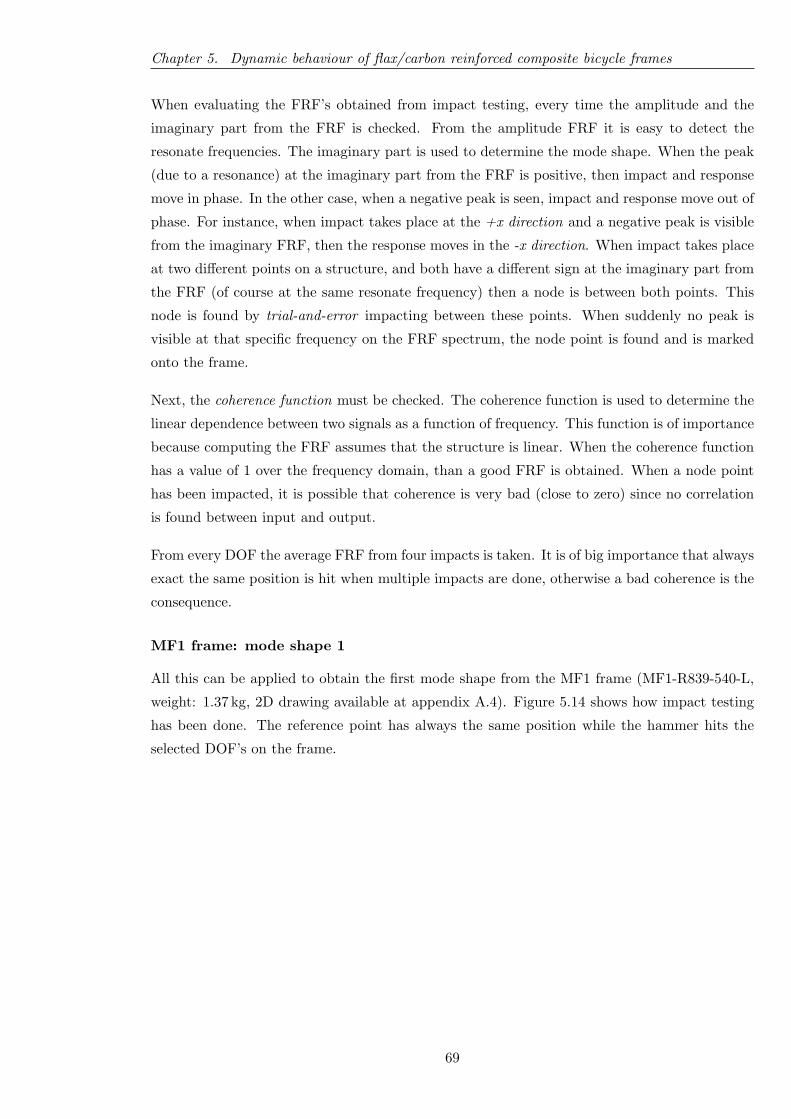
Chapter 5. Dynamic behaviour of flax/carbon reinforced composite bicycle frames
When evaluating the FRF’s obtained from impact testing, every time the amplitude and the
imaginary part from the FRF is checked. From the amplitude FRF it is easy to detect the
resonate frequencies. The imaginary part is used to determine the mode shape. When the peak
(due to a resonance) at the imaginary part from the FRF is positive, then impact and response
move in phase. In the other case, when a negative peak is seen, impact and response move out of
phase. For instance, when impact takes place at the +x direction and a negative peak is visible
from the imaginary FRF, then the response moves in the -x direction. When impact takes place
at two different points on a structure, and both have a different sign at the imaginary part from
the FRF (of course at the same resonate frequency) then a node is between both points. This
node is found by trial-and-error impacting between these points. When suddenly no peak is
visible at that specific frequency on the FRF spectrum, the node point is found and is marked
onto the frame.
Next, the coherence function must be checked. The coherence function is used to determine the
linear dependence between two signals as a function of frequency. This function is of importance
because computing the FRF assumes that the structure is linear. When the coherence function
has a value of 1 over the frequency domain, than a good FRF is obtained. When a node point
has been impacted, it is possible that coherence is very bad (close to zero) since no correlation
is found between input and output.
From every DOF the average FRF from four impacts is taken. It is of big importance that always
exact the same position is hit when multiple impacts are done, otherwise a bad coherence is the
consequence.
MF1 frame: mode shape 1
All this can be applied to obtain the first mode shape from the MF1 frame (MF1-R839-540-L,
weight: 1.37 kg, 2D drawing available at appendix A.4). Figure 5.14 shows how impact testing
has been done. The reference point has always the same position while the hammer hits the
selected DOF’s on the frame.
69
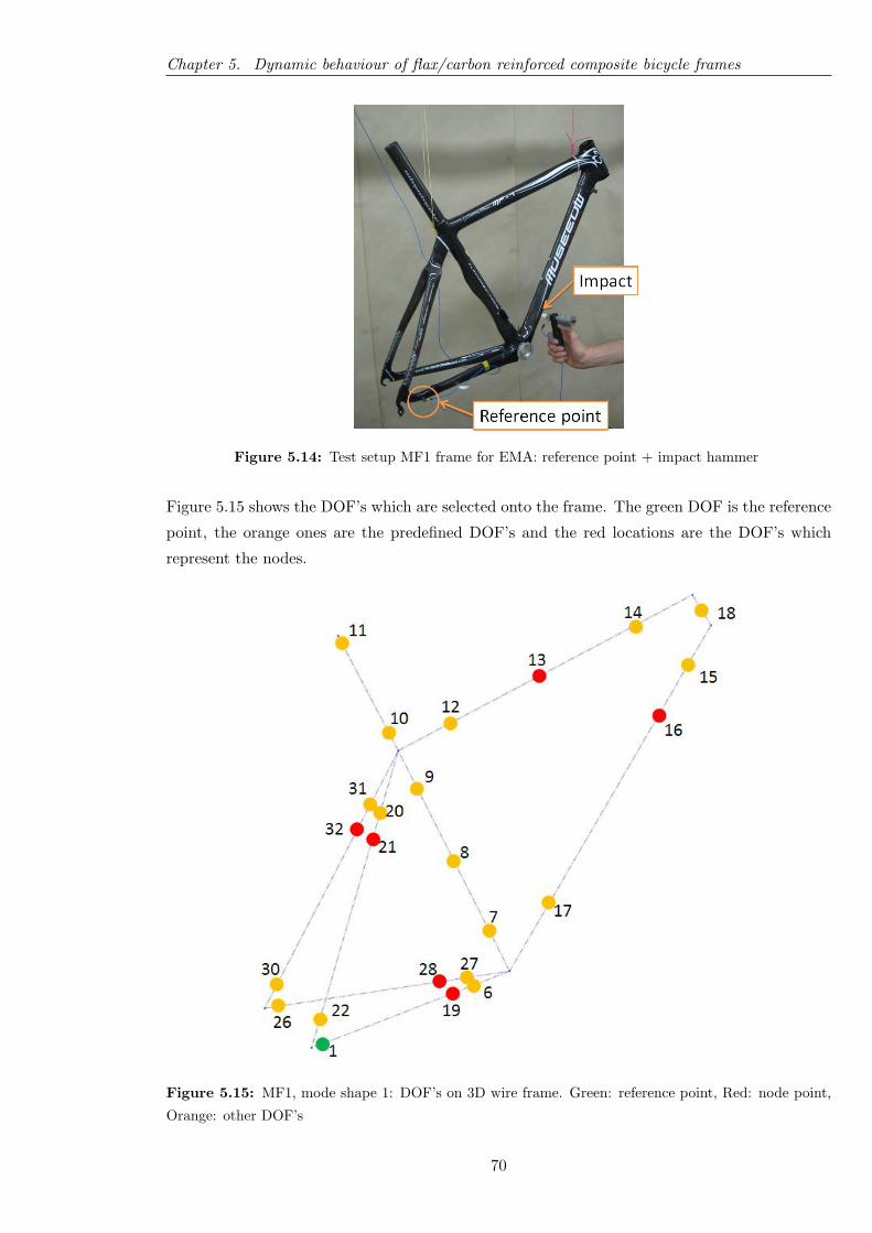
Chapter 5. Dynamic behaviour of flax/carbon reinforced composite bicycle frames
Figure 5.14: Test setup MF1 frame for EMA: reference point + impact hammer
Figure 5.15 shows the DOF’s which are selected onto the frame. The green DOF is the reference
point, the orange ones are the predefined DOF’s and the red locations are the DOF’s which
represent the nodes.
Figure 5.15: MF1, mode shape 1: DOF’s on 3D wire frame. Green: reference point, Red: node point,
Orange: other DOF’s
70
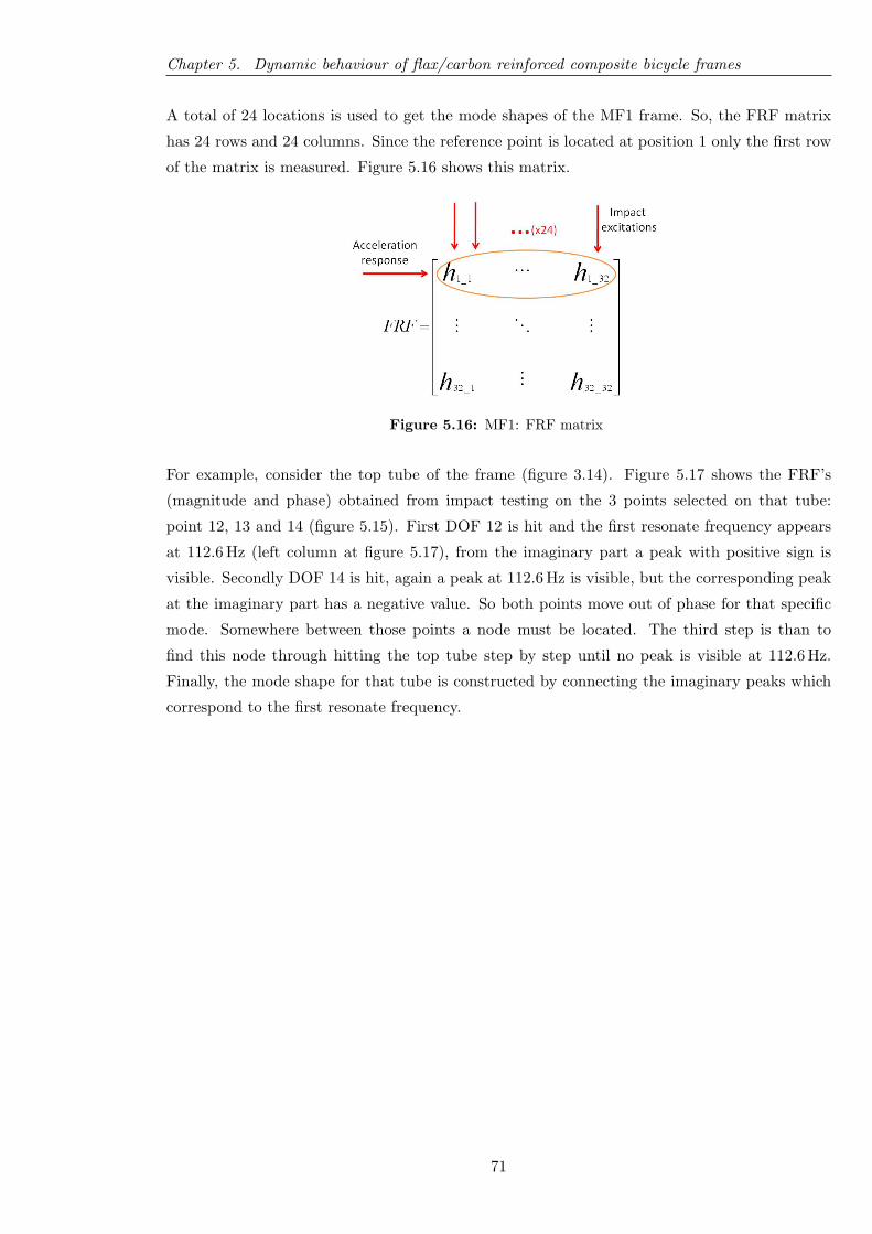
Chapter 5. Dynamic behaviour of flax/carbon reinforced composite bicycle frames
A total of 24 locations is used to get the mode shapes of the MF1 frame. So, the FRF matrix
has 24 rows and 24 columns. Since the reference point is located at position 1 only the first row
of the matrix is measured. Figure 5.16 shows this matrix.
Figure 5.16: MF1: FRF matrix
For example, consider the top tube of the frame (figure 3.14). Figure 5.17 shows the FRF’s
(magnitude and phase) obtained from impact testing on the 3 points selected on that tube:
point 12, 13 and 14 (figure 5.15). First DOF 12 is hit and the first resonate frequency appears
at 112.6 Hz (left column at figure 5.17), from the imaginary part a peak with positive sign is
visible. Secondly DOF 14 is hit, again a peak at 112.6 Hz is visible, but the corresponding peak
at the imaginary part has a negative value. So both points move out of phase for that specific
mode. Somewhere between those points a node must be located. The third step is than to
find this node through hitting the top tube step by step until no peak is visible at 112.6 Hz.
Finally, the mode shape for that tube is constructed by connecting the imaginary peaks which
correspond to the first resonate frequency.
71
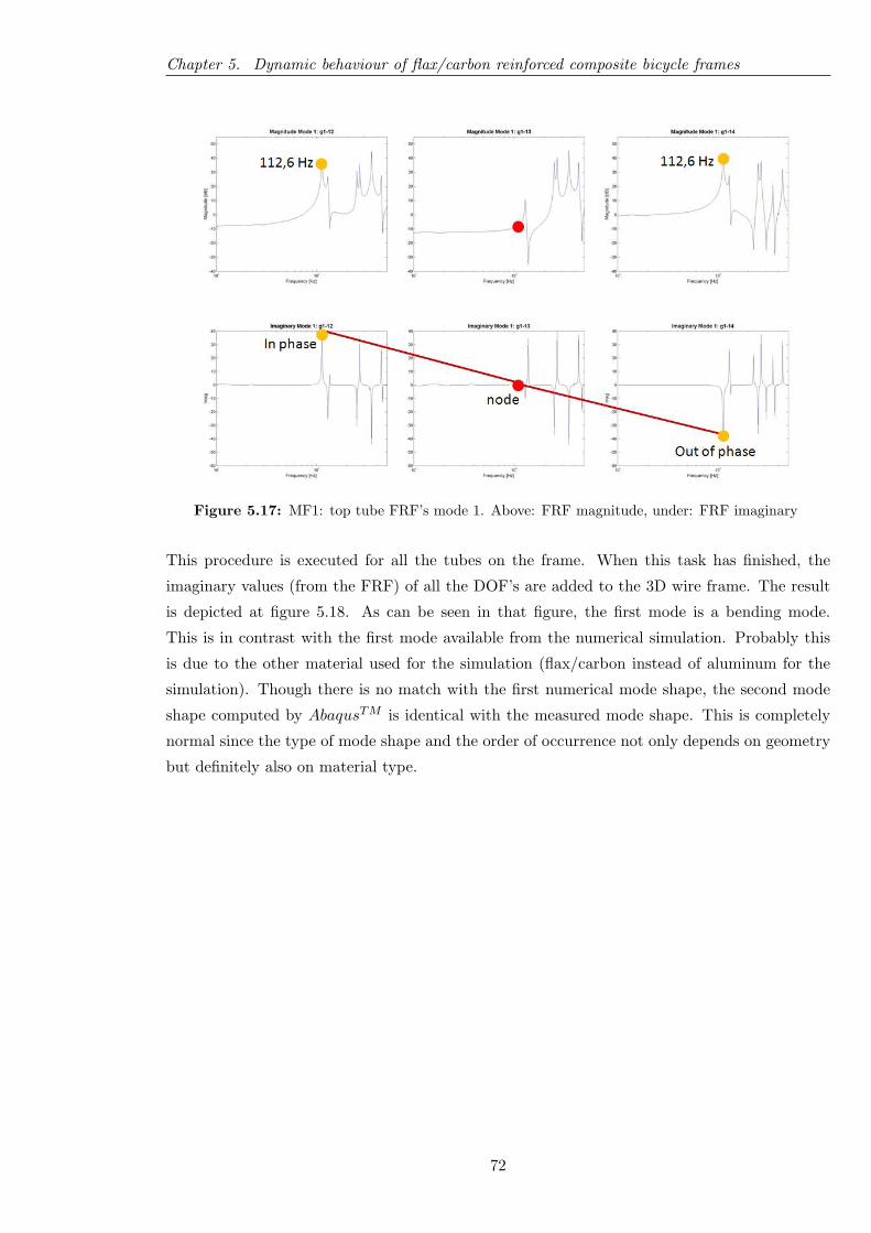
Chapter 5. Dynamic behaviour of flax/carbon reinforced composite bicycle frames
Figure 5.17: MF1: top tube FRF’s mode 1. Above: FRF magnitude, under: FRF imaginary
This procedure is executed for all the tubes on the frame. When this task has finished, the
imaginary values (from the FRF) of all the DOF’s are added to the 3D wire frame. The result
is depicted at figure 5.18. As can be seen in that figure, the first mode is a bending mode.
This is in contrast with the first mode available from the numerical simulation. Probably this
is due to the other material used for the simulation (flax/carbon instead of aluminum for the
simulation). Though there is no match with the first numerical mode shape, the second mode
shape computed by AbaqusTM is identical with the measured mode shape. This is completely
normal since the type of mode shape and the order of occurrence not only depends on geometry
but definitely also on material type.
72
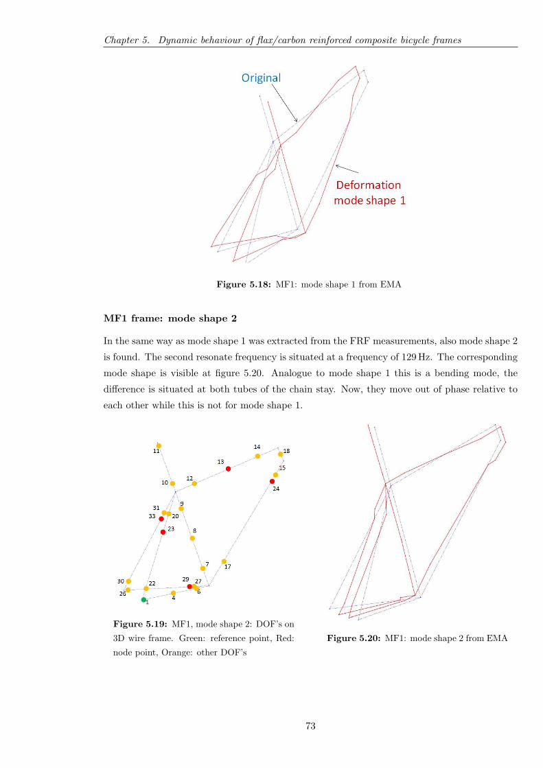
Chapter 5. Dynamic behaviour of flax/carbon reinforced composite bicycle frames
Figure 5.18: MF1: mode shape 1 from EMA
MF1 frame: mode shape 2
In the same way as mode shape 1 was extracted from the FRF measurements, also mode shape 2
is found. The second resonate frequency is situated at a frequency of 129 Hz. The corresponding
mode shape is visible at figure 5.20. Analogue to mode shape 1 this is a bending mode, the
difference is situated at both tubes of the chain stay. Now, they move out of phase relative to
each other while this is not for mode shape 1.
Figure 5.19: MF1, mode shape 2: DOF’s on
3D wire frame. Green: reference point, Red:
node point, Orange: other DOF’s
Figure 5.20: MF1: mode shape 2 from EMA
73
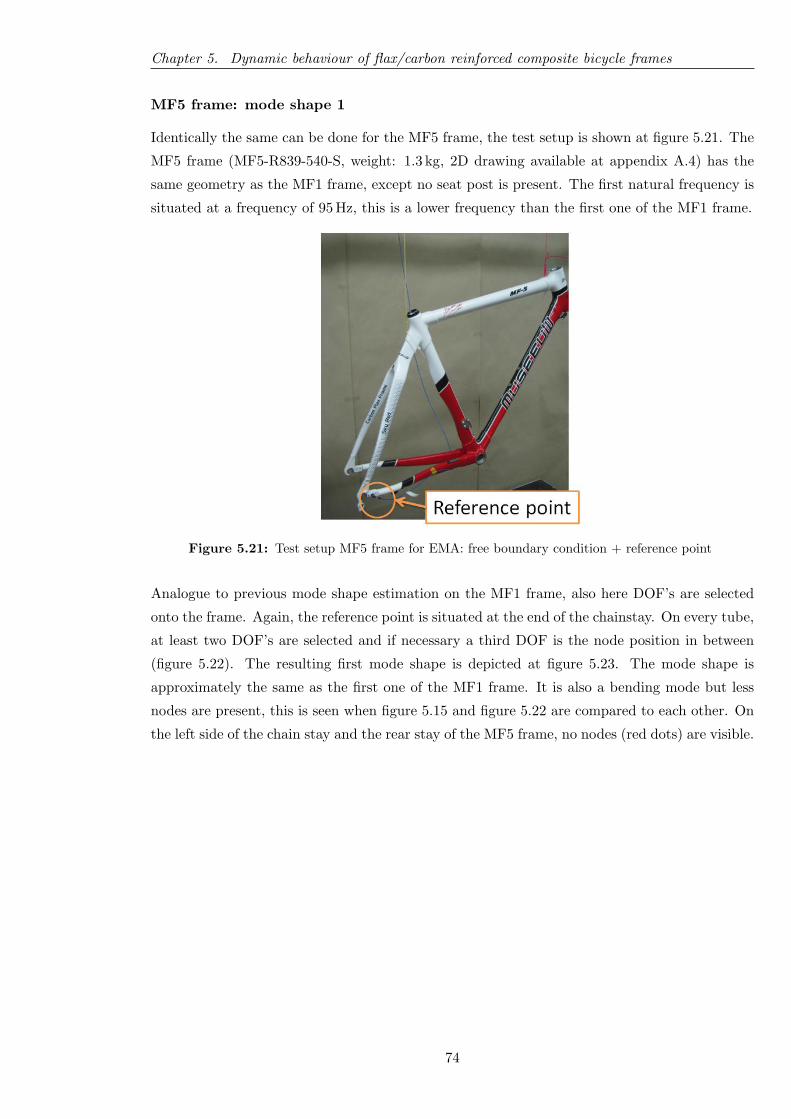
Chapter 5. Dynamic behaviour of flax/carbon reinforced composite bicycle frames
MF5 frame: mode shape 1
Identically the same can be done for the MF5 frame, the test setup is shown at figure 5.21. The
MF5 frame (MF5-R839-540-S, weight: 1.3 kg, 2D drawing available at appendix A.4) has the
same geometry as the MF1 frame, except no seat post is present. The first natural frequency is
situated at a frequency of 95 Hz, this is a lower frequency than the first one of the MF1 frame.
Figure 5.21: Test setup MF5 frame for EMA: free boundary condition + reference point
Analogue to previous mode shape estimation on the MF1 frame, also here DOF’s are selected
onto the frame. Again, the reference point is situated at the end of the chainstay. On every tube,
at least two DOF’s are selected and if necessary a third DOF is the node position in between
(figure 5.22). The resulting first mode shape is depicted at figure 5.23. The mode shape is
approximately the same as the first one of the MF1 frame. It is also a bending mode but less
nodes are present, this is seen when figure 5.15 and figure 5.22 are compared to each other. On
the left side of the chain stay and the rear stay of the MF5 frame, no nodes (red dots) are visible.
74
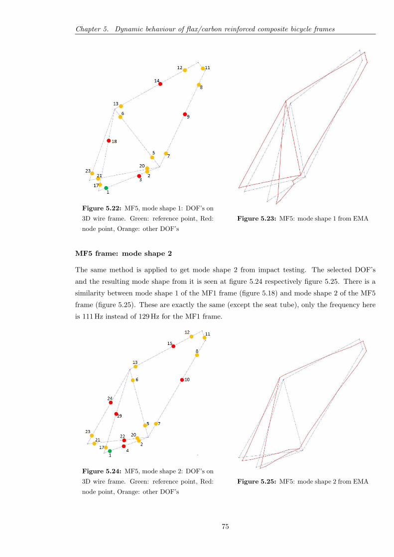
Chapter 5. Dynamic behaviour of flax/carbon reinforced composite bicycle frames
Figure 5.22: MF5, mode shape 1: DOF’s on
3D wire frame. Green: reference point, Red:
node point, Orange: other DOF’s
Figure 5.23: MF5: mode shape 1 from EMA
MF5 frame: mode shape 2
The same method is applied to get mode shape 2 from impact testing. The selected DOF’s
and the resulting mode shape from it is seen at figure 5.24 respectively figure 5.25. There is a
similarity between mode shape 1 of the MF1 frame (figure 5.18) and mode shape 2 of the MF5
frame (figure 5.25). These are exactly the same (except the seat tube), only the frequency here
is 111 Hz instead of 129 Hz for the MF1 frame.
Figure 5.24: MF5, mode shape 2: DOF’s on
3D wire frame. Green: reference point, Red:
node point, Orange: other DOF’s
Figure 5.25: MF5: mode shape 2 from EMA
75
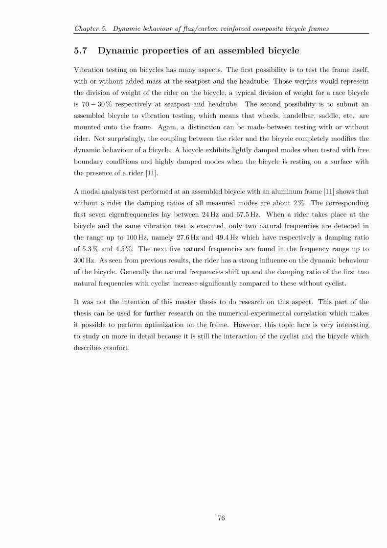
Chapter 5. Dynamic behaviour of flax/carbon reinforced composite bicycle frames
5.7 Dynamic properties of an assembled bicycle
Vibration testing on bicycles has many aspects. The first possibility is to test the frame itself,
with or without added mass at the seatpost and the headtube. Those weights would represent
the division of weight of the rider on the bicycle, a typical division of weight for a race bicycle
is 70− 30 % respectively at seatpost and headtube. The second possibility is to submit an
assembled bicycle to vibration testing, which means that wheels, handelbar, saddle, etc. are
mounted onto the frame. Again, a distinction can be made between testing with or without
rider. Not surprisingly, the coupling between the rider and the bicycle completely modifies the
dynamic behaviour of a bicycle. A bicycle exhibits lightly damped modes when tested with free
boundary conditions and highly damped modes when the bicycle is resting on a surface with
the presence of a rider [11].
A modal analysis test performed at an assembled bicycle with an aluminum frame [11] shows that
without a rider the damping ratios of all measured modes are about 2 %. The corresponding
first seven eigenfrequencies lay between 24 Hz and 67.5 Hz. When a rider takes place at the
bicycle and the same vibration test is executed, only two natural frequencies are detected in
the range up to 100 Hz, namely 27.6 Hz and 49.4 Hz which have respectively a damping ratio
of 5.3 % and 4.5 %. The next five natural frequencies are found in the frequency range up to
300 Hz. As seen from previous results, the rider has a strong influence on the dynamic behaviour
of the bicycle. Generally the natural frequencies shift up and the damping ratio of the first two
natural frequencies with cyclist increase significantly compared to these without cyclist.
It was not the intention of this master thesis to do research on this aspect. This part of the
thesis can be used for further research on the numerical-experimental correlation which makes
it possible to perform optimization on the frame. However, this topic here is very interesting
to study on more in detail because it is still the interaction of the cyclist and the bicycle which
describes comfort.
76
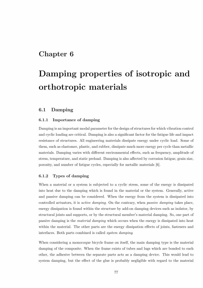
Chapter 6
Damping properties of isotropic and
orthotropic materials
6.1 Damping
6.1.1 Importance of damping
Damping is an important modal parameter for the design of structures for which vibration control
and cyclic loading are critical. Damping is also a significant factor for the fatigue life and impact
resistance of structures. All engineering materials dissipate energy under cyclic load. Some of
them, such as elastomer, plastic, and rubber, dissipate much more energy per cycle than metallic
materials. Damping varies with different environmental effects, such as frequency, amplitude of
stress, temperature, and static preload. Damping is also affected by corrosion fatigue, grain size,
porosity, and number of fatigue cycles, especially for metallic materials [6].
6.1.2 Types of damping
When a material or a system is subjected to a cyclic stress, some of the energy is dissipated
into heat due to the damping which is found in the material or the system. Generally, active
and passive damping can be considered. When the energy from the system is dissipated into
controlled actuators, it is active damping. On the contrary, when passive damping takes place,
energy dissipation is found within the structure by add-on damping devices such as isolator, by
structural joints and supports, or by the structural member’s material damping. So, one part of
passive damping is the material damping which occurs when the energy is dissipated into heat
within the material. The other parts are the energy dissipation effects of joints, fasteners and
interfaces. Both parts combined is called system damping.
When considering a monocoque bicycle frame on itself, the main damping type is the material
damping of the composite. When the frame exists of tubes and lugs which are bonded to each
other, the adhesive between the separate parts acts as a damping device. This would lead to
system damping, but the effect of the glue is probably negligible with regard to the material
77

Chapter 6. Damping properties of isotropic and orthotropic materials
damping. On the contrary, when an assembled bicycle is considered, much more damping devices
are added such as the friction in the bearings. Also the bicyclist sitting on the bicycle shall play
a distinct role when damping must be determined.
6.1.3 Composite damping
Material damping in fibre-reinforced polymer composites is a very complicated phenomenon,
as it is not only determined by the damping properties of fibres and matrix, but also by the
fibre/matrix interphase and by material imperfections such as voids, air and moisture inclusions,
cracks, delaminations, etc. fibre-reinforced composite materials have inherent material damping
because of fibre-matrix interaction which is usually more than that of the conventional isotropic
materials.
The damped behaviour is attributed to energy dissipation because of the shear stresses between
the various fibrous strands that are kept in place by constraining viscoelastic layers. The main
source of mechanical damping in laminated composite materials is attributed to the inelastic
nature of the matrix, relative slipping at the fibre/matrix interfaces, damping due to damage
and viscoplastic damping. The damping capacity of composite laminates can be increased many
times by incorporating viscoelastic damping layers between the laminae of the composites. In
this hybrid approach, the dominant damping mechanism is the shear which is induced between
the damping layer and the constraining layers [31].
6.1.4 Damping models
One way of modeling damping is by using of the viscous damping model, where the damping is
modeled as a force proportional and synchronous with the velocity of the object but opposite in
direction to it: F = −cx. here c is the viscous damping coefficient [Ns/m] and x the velocity
[m/s]. This type of damping is found at vibrations in the air, water, oil, etc. [7]. Another
possibility to modal damping is the hysteretic damping model or structural damping model.
This type of damping is due to internal friction of the material during deformation. The friction
forces are created by slipping and sliding of internal faces over each other [7]. The internal
damping is described by a force proportional to the displacement but in phase with the velocity,
the differential equation in case of free motion and SDOF becomes: mx+hxi+kx = 0. Where h
is the hysteretic damping coefficient and i is the imaginary unit which is required to synchronize
the damping force to the velocity. When h is replaced by kη where η is the hysteretic damping
ratio which is the fraction of energy lost in every cycle of the vibration, the equation of motion
is written as: mx+k(1 +ηi)x = 0. This model reproduces the real behaviour of many vibrating
structures more closely than the viscous model. The last damping model is Coulomb-damping
[7], the friction force is a consequence of dry friction of surfaces over each other. The force
N normal to the gliding surface and the kinematic friction constant µ form the friction force
F = µN .
78
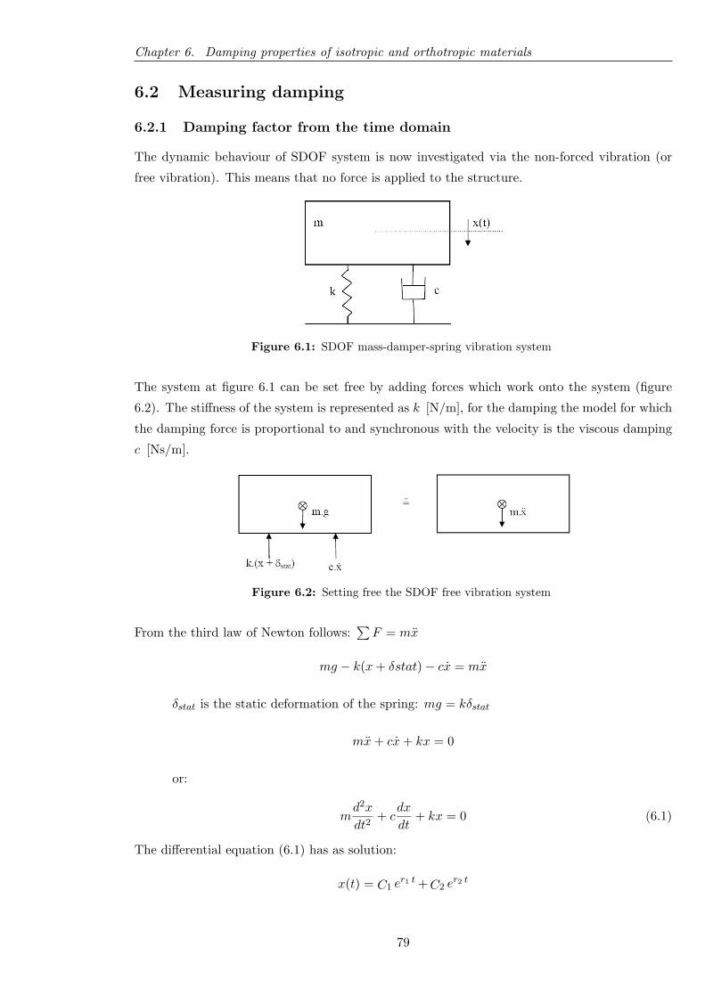
Chapter 6. Damping properties of isotropic and orthotropic materials
6.2 Measuring damping
6.2.1 Damping factor from the time domain
The dynamic behaviour of SDOF system is now investigated via the non-forced vibration (or
free vibration). This means that no force is applied to the structure.
Figure 6.1: SDOF mass-damper-spring vibration system
The system at figure 6.1 can be set free by adding forces which work onto the system (figure
6.2). The stiffness of the system is represented as k [N/m], for the damping the model for which
the damping force is proportional to and synchronous with the velocity is the viscous damping
c [Ns/m].
Figure 6.2: Setting free the SDOF free vibration system
From the third law of Newton follows:∑F = mx
mg − k(x+ δstat)− cx = mx
δstat is the static deformation of the spring: mg = kδstat
mx+ cx+ kx = 0
or:
md2x
dt2+ c
dx
dt+ kx = 0 (6.1)
The differential equation (6.1) has as solution:
x(t) = C1 er1 t +C2 e
r2 t
79
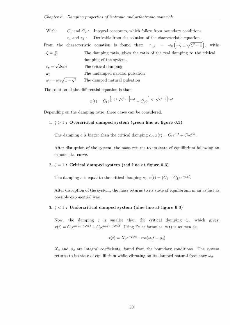
Chapter 6. Damping properties of isotropic and orthotropic materials
With: C1 and C2 : Integral constants, which follow from boundary conditions.
r1 and r2 : Derivable from the solution of the characteristic equation.
From the characteristic equation is found that: r1,2 = ω0
(−ζ ±
√ζ2 − 1
), with:
ζ = ccc
The damping ratio, gives the ratio of the real damping to the critical
damping of the system.
cc =√
2km The critical damping
ω0 The undamped natural pulsation
ωd = ω0
√1− ζ2 The damped natural pulsation
The solution of the differential equation is than:
x(t) = C1e
[−ζ+√ζ2−1
]ω0t + C2e
[−ζ−√ζ2−1
]ω0t
Depending on the damping ratio, three cases can be considered.
1. ζ > 1 : Overcritical damped system (green line at figure 6.3)
The damping c is bigger than the critical damping cc, x(t) = C1er1t + C2e
r2t.
After disruption of the system, the mass returns to its state of equilibrium following an
exponential curve.
2. ζ = 1 : Critical damped system (red line at figure 6.3)
The damping c is equal to the critical damping cc, x(t) = (C1 + C2) e−ω0t.
After disruption of the system, the mass returns to its state of equilibrium in an as fast as
possible exponential way.
3. ζ < 1 : Undercritical damped system (blue line at figure 6.3)
Now, the damping c is smaller than the critical damping cc, which gives:
x(t) = C1eω0ζt+jω0ζt + C2e
ω0ζt−jω0ζt. Using Euler formulas, x(t) is written as:
x(t) = Xde−ζω0t · cos(ωdt− φd)
Xd and φd are integral coefficients, found from the boundary conditions. The system
returns to its state of equilibrium while vibrating on its damped natural frequency ωd.
80
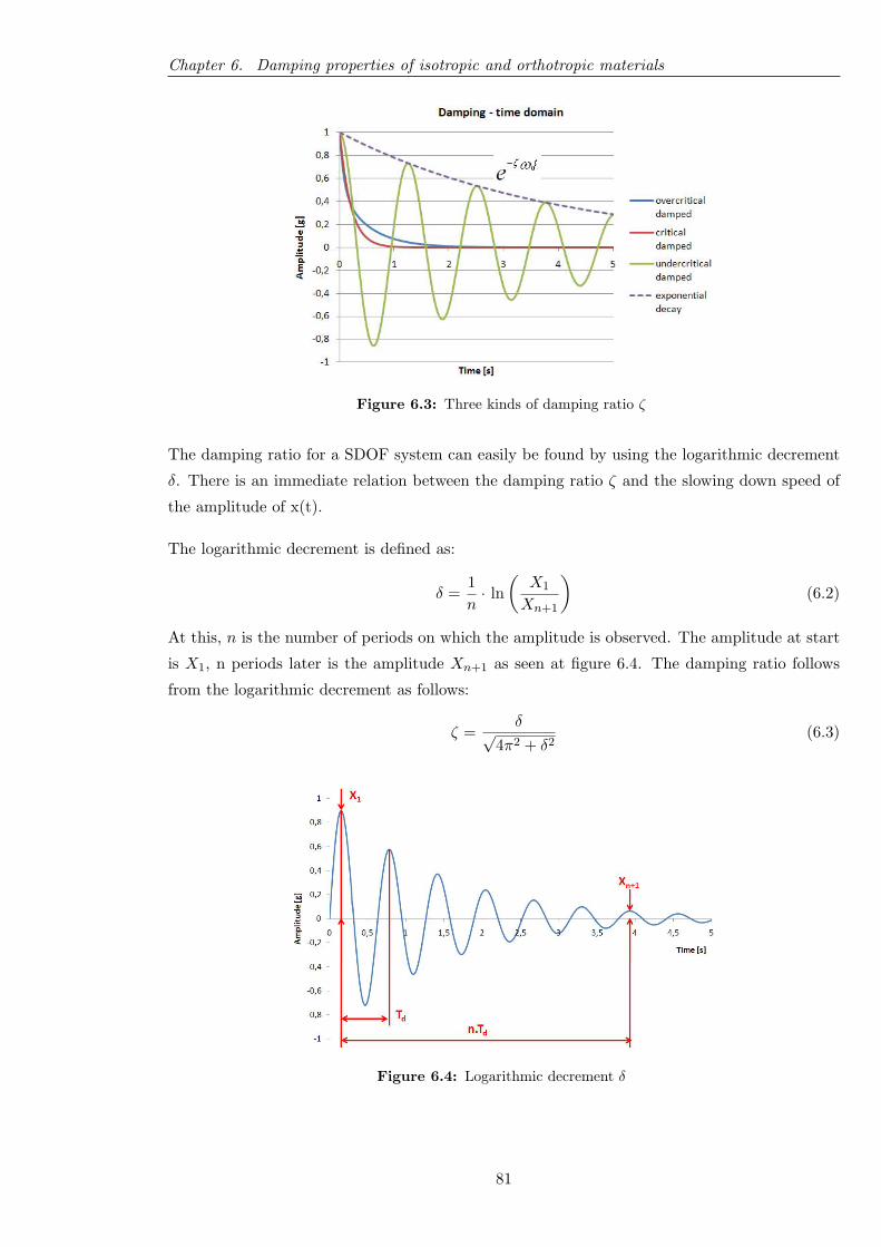
Chapter 6. Damping properties of isotropic and orthotropic materials
Figure 6.3: Three kinds of damping ratio ζ
The damping ratio for a SDOF system can easily be found by using the logarithmic decrement
δ. There is an immediate relation between the damping ratio ζ and the slowing down speed of
the amplitude of x(t).
The logarithmic decrement is defined as:
δ =1n
· ln(
X1
Xn+1
)(6.2)
At this, n is the number of periods on which the amplitude is observed. The amplitude at start
is X1, n periods later is the amplitude Xn+1 as seen at figure 6.4. The damping ratio follows
from the logarithmic decrement as follows:
ζ =δ√
4π2 + δ2(6.3)
Figure 6.4: Logarithmic decrement δ
81

Chapter 6. Damping properties of isotropic and orthotropic materials
6.2.2 Damping factor from the frequency domain
The previous method measures the damping in the time domain. Another possibility is to get
the damping factor from the frequency domain, it is called the half-power bandwidth method.
First the FRF must be obtained. Corresponding to a resonate frequency, a peak is visible in
the FRF spectrum. The two frequencies at the curve which correspond with the −3 dB points
down from the peak are the half power points as shown at figure 6.5. The greater f2− f1 is, the
higher the damping for that specific natural frequency. The damping loss factor η is defined as:
η = 2 · ζ =f2 − f1f0
ζ =f2 − f1
2f0
Figure 6.5: Measuring damping - half power bandwidth
Those two methods can accurately be used when the system is a SDOF vibration system, this
means that only one resonate frequency occurs and thus one peak is visible at the FRF spectrum
or when the resonate frequencies are well separated. Very often, a MDOF system is present and
thus both models cannot be used accurately anymore. However, the result from these SDOF
methods can be used as a rough estimate.
6.3 Damping properties from shaker excitation: method 1
The goal of this part of the master thesis is to assess the material damping of different materials.
Within this scope, both isotropic and orthotropic materials are subjected to a shock excitation
generated by the shaker. For this kind of test, it is important that the geometry of the samples
is always the same and that also the shock can be reproduced exactly.
6.3.1 Test setup
As illustrated in figure 6.6, the test sample is clamped onto the armature of the shaker. The
clamping system exists of two aluminum plates where the test sample is between. With four
82
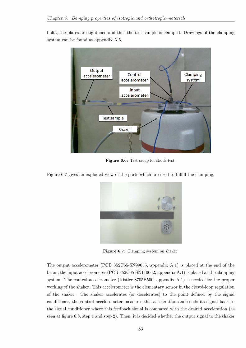
Chapter 6. Damping properties of isotropic and orthotropic materials
bolts, the plates are tightened and thus the test sample is clamped. Drawings of the clamping
system can be found at appendix A.5.
Figure 6.6: Test setup for shock test
Figure 6.7 gives an exploded view of the parts which are used to fulfill the clamping.
Figure 6.7: Clamping system on shaker
The output accelerometer (PCB 352C65-SN99055, appendix A.1) is placed at the end of the
beam, the input accelerometer (PCB 352C65-SN110062, appendix A.1) is placed at the clamping
system. The control accelerometer (Kistler 8705B500, appendix A.1) is needed for the proper
working of the shaker. This accelerometer is the elementary sensor in the closed-loop regulation
of the shaker. The shaker accelerates (or decelerates) to the point defined by the signal
conditioner, the control accelerometer measures this acceleration and sends its signal back to
the signal conditioner where this feedback signal is compared with the desired acceleration (as
seen at figure 6.8, step 1 and step 2). Then, it is decided whether the output signal to the shaker
83
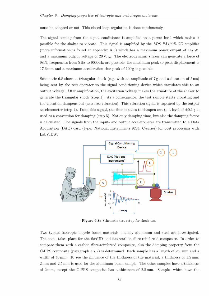
Chapter 6. Damping properties of isotropic and orthotropic materials
must be adapted or not. This closed-loop regulation is done continuously.
The signal coming from the signal conditioner is amplified to a power level which makes it
possible for the shaker to vibrate. This signal is amplified by the LDS PA100E-CE amplifier
(more information is found at appendix A.3) which has a maximum power output of 147 W,
and a maximum output voltage of 20 Vrms. The electrodynamic shaker can generate a force of
98 N, frequencies from 5 Hz to 9000 Hz are possible, the maximum peak to peak displacement is
17.6 mm and a maximum acceleration sine peak of 100 g is possible.
Schematic 6.8 shows a triangular shock (e.g. with an amplitude of 7 g and a duration of 5 ms)
being sent by the test operator to the signal conditioning device which translates this to an
output voltage. After amplification, the excitation voltage makes the armature of the shaker to
generate the triangular shock (step 1). As a consequence, the test sample starts vibrating and
the vibration dampens out (as a free vibration). This vibration signal is captured by the output
accelerometer (step 4). From this signal, the time it takes to dampen out to a level of ±0.1 g is
used as a convention for damping (step 5). Not only damping time, but also the damping factor
is calculated. The signals from the input- and output accelerometer are transmitted to a Data
Acquisition (DAQ) card (type: National Instruments 9234, C-series) for post processing with
LabVIEW.
Figure 6.8: Schematic test setup for shock test
Two typical isotropic bicycle frame materials, namely aluminum and steel are investigated.
The same takes place for the flaxUD and flax/carbon fibre-reinforced composite. In order to
compare them with a carbon fibre-reinforced composite, also the damping property from the
C-PPS composite (paragraph 4.7.2) is determined. Each sample has a length of 250 mm and a
width of 40 mm. To see the influence of the thickness of the material, a thickness of 1.5 mm,
2 mm and 2.5 mm is used for the aluminum beam sample. The other samples have a thickness
of 2 mm, except the C-PPS composite has a thickness of 2.5 mm. Samples which have the
84
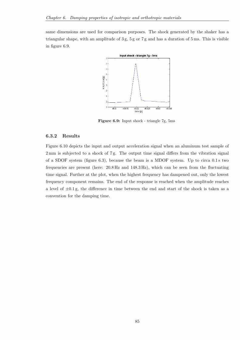
Chapter 6. Damping properties of isotropic and orthotropic materials
same dimensions are used for comparison purposes. The shock generated by the shaker has a
triangular shape, with an amplitude of 3 g, 5 g or 7 g and has a duration of 5 ms. This is visible
in figure 6.9.
Figure 6.9: Input shock - triangle 7g, 5ms
6.3.2 Results
Figure 6.10 depicts the input and output acceleration signal when an aluminum test sample of
2 mm is subjected to a shock of 7 g. The output time signal differs from the vibration signal
of a SDOF system (figure 6.3), because the beam is a MDOF system. Up to circa 0.1 s two
frequencies are present (here: 20.8 Hz and 148.3 Hz), which can be seen from the fluctuating
time signal. Further at the plot, when the highest frequency has dampened out, only the lowest
frequency component remains. The end of the response is reached when the amplitude reaches
a level of ±0.1 g, the difference in time between the end and start of the shock is taken as a
convention for the damping time.
85

Chapter 6. Damping properties of isotropic and orthotropic materials
Figure 6.10: Input and output signal from shock excitation
For all samples three iterations were done, and every time the damping time and damping factor
is calculated. From these three measurements, the average is taken of which table 6.1 gives an
overview. The variation on damping time from these three measurement is very small (less than
5 %). From table 6.1 it is seen that the damping time of steel (2 mm)is approximately the half
of that of aluminum (2 mm). When the samples with equal dimensions are compared with each
other, steel has the best damping over aluminum respectively flaxUD. The damping time from
aluminum is also less than that of the C-PPS composite, resulting from the comparison between
the samples of 2.5 mm. A different fibre direction leads to another damping time, as can be
concluded from the C-PPS composite.
86
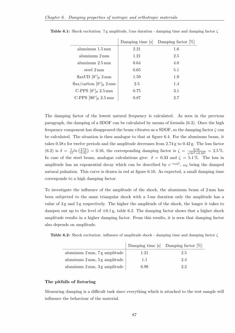
Chapter 6. Damping properties of isotropic and orthotropic materials
Table 6.1: Shock excitation: 7 g amplitude, 5 ms duration - damping time and damping factor ζ
Damping time [s] Damping factor [%]
aluminum 1.5 mm 2.21 1.6
aluminum 2 mm 1.21 2.5
aluminum 2.5 mm 0.64 4.0
steel 2 mm 0.65 5.1
flaxUD [0◦]8 2 mm 1.59 1.9
flax/carbon [0◦]6 2 mm 2.5 1.4
C-PPS [0◦]8 2.5 mm 0.75 3.1
C-PPS [90◦]8 2.5 mm 0.87 2.7
The damping factor of the lowest natural frequency is calculated. As seen in the previous
paragraph, the damping of a SDOF can be calculated by means of formula (6.3). Once the high
frequency component has disappeared the beam vibrates as a SDOF, so the damping factor ζ can
be calculated. The situation is then analogue to that at figure 6.4. For the aluminum beam, it
takes 0.58 s for twelve periods and the amplitude decreases from 2.74 g to 0.42 g. The loss factor
(6.2) is δ = 112 ln
(2.740.42
)= 0.16, the corresponding damping factor is ζ = 0.16√
4π2+0.162= 2.5 %.
In case of the steel beam, analogue calculations give: δ = 0.33 and ζ = 5.1 %. The loss in
amplitude has an exponential decay which can be described by e−ωdζt, ωd being the damped
natural pulsation. This curve is drawn in red at figure 6.10. As expected, a small damping time
corresponds to a high damping factor.
To investigate the influence of the amplitude of the shock, the aluminum beam of 2 mm has
been subjected to the same triangular shock with a 5 ms duration only the amplitude has a
value of 3 g and 5 g respectively. The higher the amplitude of the shock, the longer it takes to
dampen out up to the level of ±0.1 g, table 6.2. The damping factor shows that a higher shock
amplitude results in a higher damping factor. From this results, it is seen that damping factor
also depends on amplitude.
Table 6.2: Shock excitation: influence of amplitude shock - damping time and damping factor ζ
Damping time [s] Damping factor [%]
aluminum 2 mm, 7 g amplitude 1.21 2.5
aluminum 2 mm, 5 g amplitude 1.1 2.4
aluminum 2 mm, 3 g amplitude 0.98 2.2
The pitfalls of fixturing
Measuring damping is a difficult task since everything which is attached to the test sample will
influence the behaviour of the material.
87

Chapter 6. Damping properties of isotropic and orthotropic materials
Pitfall 1
The mass of the response accelerometer (5 g) will have an influence on the measured dynamic
properties of the material, especially when the mass of the accelerometer is relative high
compared to the tested structure. Within this test setup, there is no other possibility to measure
the output response. A more serious problem is the cable which connects the accelerometer
with the DAQ device. As can be seen at figure 6.6, the cable is attached to the sample with
tape. This is a good method of fixing the cable because this tape prevents the cable to oscillate
when the shock takes place.
Figures 6.11(a) and 6.11(b) show how the cable may not be fixed. On both figures, the cable
of the sensor is suspended on a cord. The first test setup shows that the point of suspension
is close to the accelerometer. The second one shows that the point of suspension is far away
from the accelerometer. In both cases, the cable will oscillate when the shock takes place. As a
result, this has a very big influence on the damping time (and damping factor). The damping
factor corresponding to the test setup with the short cable is 3.5 %, the other test setup has a
damping factor of 5.4 %. Normally, with the cable attached to the sample, the damping factor
is 2.5 %. So, it is obvious that the method of fixing the accelerometer is of big importance when
doing vibrational analysis, and more specific when measuring damping.
(a) Method 1: cable too short (b) Method 2: cable too long
Figure 6.11: Fixing the accelerometer: wrong methods
Pitfall 2
The next difficulty is to realize the clamping. Here, the clamping system exists of two identical
aluminum plates, where the test sample is put in between, which are pinned to each other with
two bolts near both sides of the test sample. Finally this clamping system is connected to the
armature of the shaker, which is visible at figure 6.6. When the bolts are tightened, the upper
plate from the clamping system bends. As a consequence, not the total surface of the test sample
is prevented to move (which must be the case for a clamped beam). This situation is sketched
in figure 6.12.
88
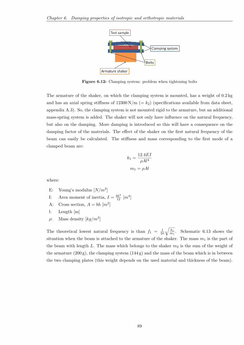
Chapter 6. Damping properties of isotropic and orthotropic materials
Figure 6.12: Clamping system: problem when tightening bolts
The armature of the shaker, on which the clamping system is mounted, has a weight of 0.2 kg
and has an axial spring stiffness of 12300 N/m (= k2) (specifications available from data sheet,
appendix A.3). So, the clamping system is not mounted rigid to the armature, but an additional
mass-spring system is added. The shaker will not only have influence on the natural frequency,
but also on the damping. More damping is introduced so this will have a consequence on the
damping factor of the materials. The effect of the shaker on the first natural frequency of the
beam can easily be calculated. The stiffness and mass corresponding to the first mode of a
clamped beam are:
k1 =12.4EIρAl4
m1 = ρAl
where:
E: Young’s modulus [N/m2]
I: Area moment of inertia, I = bh3
12 [m4]
A: Cross section, A = bh [m2]
l: Length [m]
ρ: Mass density [kg/m3]
The theoretical lowest natural frequency is than f1 = 12π
√k1m1
. Schematic 6.13 shows the
situation when the beam is attached to the armature of the shaker. The mass m1 is the part of
the beam with length L. The mass which belongs to the shaker m2 is the sum of the weight of
the armature (200 g), the clamping system (144 g) and the mass of the beam which is in between
the two clamping plates (this weight depends on the used material and thickness of the beam).
89

Chapter 6. Damping properties of isotropic and orthotropic materials
Figure 6.13: Schematic from clamped beam + shaker
When writing down the kinetic and potential energy from this system (which has 2 DOF’s), the
mass matrix [M] and the stiffness matrix [K] are:
[M ] =
[m1 0
0 m2
]
[K] =
[k1 −k1
−k1 k1 + k2
]
Because there are 2 DOF’s, also 2 natural frequencies are found.
det[[K]− ω2[M ]
]= 0
k1k2 − k1ω2m2 − ω2m1k1 − ω2m1k2 + ω4m1m2 = 0 (6.4)
ω1 = . . . [rad/s]
ω2 = . . . [rad/s]
The results of this formula for the steel and aluminum beams are given in table 6.3. The first
column gives the natural frequency when the clamping system would be perfect. The second
column is ω1 from equation (6.4). The last column is the measured lowest natural frequency,
which follows from FFT calculation of the response signal.
Table 6.3: Measured and calculated natural frequency for first mode: influence of shaker
Theoretical clamped Theoretical Clamped beam Measured
beam [Hz] + shaker [Hz] [Hz]
aluminum 1.5 mm 19.8 19 15.9
aluminum 2 mm 26.4 23 20.6
aluminum 2.5 mm 32.9 24.7 24.3
steel 2 mm 26.9 20.4 18.4
It is clear that the effect of the shaker results in a lower calculated frequency (column 1 compared
to column 2) and the measured frequency is always lower than the calculated (column 2 compared
90

Chapter 6. Damping properties of isotropic and orthotropic materials
to column 3). The difference between measured and calculated frequency can be due to the
inefficient clamping system (figure 6.12). Another possible reason is that the armature does not
only make an axial movement, but also has a transversal deflection due to the bending force
which acts onto the armature because of non-symmetrical clamping of the beam onto the shaker.
6.4 Damping properties from shaker excitation: method 2
6.4.1 Test setup
The previous method has as disadvantages that the clamping can not be totally fulfilled and
also the force which works onto the sample is not measured. Measuring force is preferred over
acceleration as input signal, because a constant acceleration amplitude of the triangular shock
for different materials of the test samples leads to another force which is put onto the test
sample. For example, a steel beam is heavier than an aluminum beam, as a result the steel
beam is subjected to a higher force amplitude which can result in misleading results. Because
of these reasons, another fixing system to measure damping is designed: it should eliminate the
clamping system (based on tightening of two plates) and also being able to measure the force.
First of all a symmetric test sample is used, so the armature of the shaker is not subjected to
a bending load anymore. Next in order to measure the force of the shaker, a force sensor is
placed between the armature of the shaker and the new clamping system. At last, instead of a
big contact area (clamping system/test sample), a line contact is used to realize the clamping.
The result from all of these modifications is visible at figure 6.14. To measure the response,
accelerometers are still being used, but they are mounted in such way that symmetry is still
there. The line contact is achieved by using two V-shaped parts which are tightened with four
bolts (drawings available at appendix A.5).
Figure 6.14: Symmetric fixture system
An exploded view of the clamping system is depicted at figure 6.15.
91
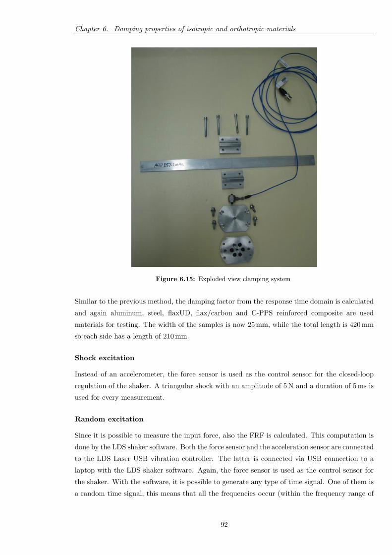
Chapter 6. Damping properties of isotropic and orthotropic materials
Figure 6.15: Exploded view clamping system
Similar to the previous method, the damping factor from the response time domain is calculated
and again aluminum, steel, flaxUD, flax/carbon and C-PPS reinforced composite are used
materials for testing. The width of the samples is now 25 mm, while the total length is 420 mm
so each side has a length of 210 mm.
Shock excitation
Instead of an accelerometer, the force sensor is used as the control sensor for the closed-loop
regulation of the shaker. A triangular shock with an amplitude of 5 N and a duration of 5 ms is
used for every measurement.
Random excitation
Since it is possible to measure the input force, also the FRF is calculated. This computation is
done by the LDS shaker software. Both the force sensor and the acceleration sensor are connected
to the LDS Laser USB vibration controller. The latter is connected via USB connection to a
laptop with the LDS shaker software. Again, the force sensor is used as the control sensor for
the shaker. With the software, it is possible to generate any type of time signal. One of them is
a random time signal, this means that all the frequencies occur (within the frequency range of
92
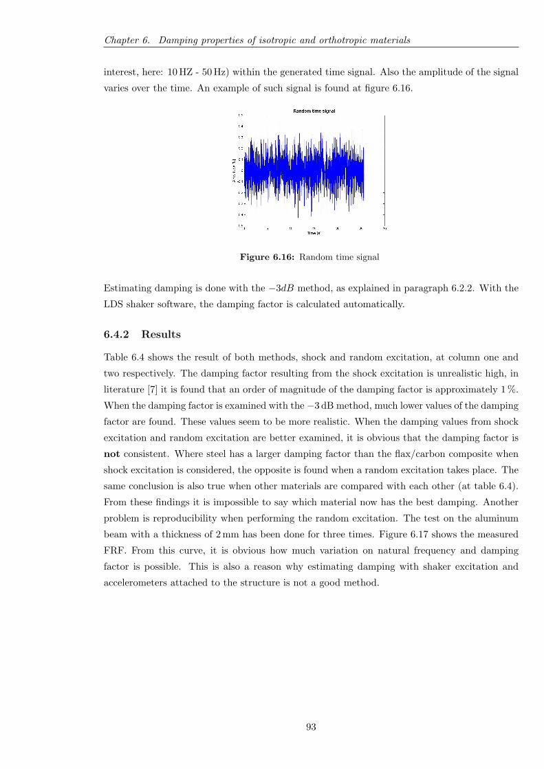
Chapter 6. Damping properties of isotropic and orthotropic materials
interest, here: 10 HZ - 50 Hz) within the generated time signal. Also the amplitude of the signal
varies over the time. An example of such signal is found at figure 6.16.
Figure 6.16: Random time signal
Estimating damping is done with the −3dB method, as explained in paragraph 6.2.2. With the
LDS shaker software, the damping factor is calculated automatically.
6.4.2 Results
Table 6.4 shows the result of both methods, shock and random excitation, at column one and
two respectively. The damping factor resulting from the shock excitation is unrealistic high, in
literature [7] it is found that an order of magnitude of the damping factor is approximately 1 %.
When the damping factor is examined with the −3 dB method, much lower values of the damping
factor are found. These values seem to be more realistic. When the damping values from shock
excitation and random excitation are better examined, it is obvious that the damping factor is
not consistent. Where steel has a larger damping factor than the flax/carbon composite when
shock excitation is considered, the opposite is found when a random excitation takes place. The
same conclusion is also true when other materials are compared with each other (at table 6.4).
From these findings it is impossible to say which material now has the best damping. Another
problem is reproducibility when performing the random excitation. The test on the aluminum
beam with a thickness of 2 mm has been done for three times. Figure 6.17 shows the measured
FRF. From this curve, it is obvious how much variation on natural frequency and damping
factor is possible. This is also a reason why estimating damping with shaker excitation and
accelerometers attached to the structure is not a good method.
93
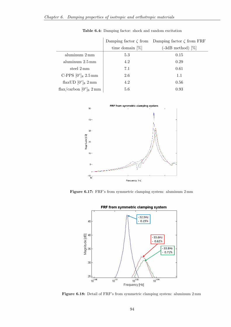
Chapter 6. Damping properties of isotropic and orthotropic materials
Table 6.4: Damping factor: shock and random excitation
Damping factor ζ from Damping factor ζ from FRF
time domain [%] (-3dB method) [%]
aluminum 2 mm 5.3 0.15
aluminum 2.5 mm 4.2 0.29
steel 2 mm 7.1 0.61
C-PPS [0◦]8 2.5 mm 2.6 1.1
flaxUD [0◦]8 2 mm 4.2 0.56
flax/carbon [0◦]6 2 mm 5.6 0.93
Figure 6.17: FRF’s from symmetric clamping system: aluminum 2 mm
Figure 6.18: Detail of FRF’s from symmetric clamping system: aluminum 2 mm
94

Chapter 6. Damping properties of isotropic and orthotropic materials
6.5 Damping properties from acoustic wave excitation
From the previous sections it is obvious that determining damping is not an easy task.
Everything which is attached to the structure under test will have an influence on the
damping. Previously, excitation took place with a shaker and response was measured with
an accelerometer. Every time these items were attached to the structure, so they have a
(big) influence on the damping. So, based on these findings it should be better if excitation
and response were achieved without making contact. Excitation can be done by means of an
acoustic wave, coming from a loudspeaker. This is called acoustic wave excitation. Contactless
measuring the response is done by means of a laser vibrometer, this device is able to measure
velocity through pointing a laser beam on the structure. Thus, excitation and response are
done in a contactless way. The only thing left is the structure itself, again it is recommended
to realize a free boundary condition. The best way to do this is by suspending the test piece in
the nodes of the vibration mode of interest because at that points no vibration is present. In
case of the plate visible at figure 4.27, the cords must be attached at the middle of a side.
6.5.1 Test setup
The test setup used at the lab is shown at picture 6.19.
Figure 6.19: Test setup for acoustic wave excitation and contactless response measuring
A laser beam is pointed at the corner of a test piece, here a small flaxUD plate. The loudspeaker
is a 150 W woofer which has a frequency range of 60 Hz up to 6.5 kHz. The excitation signal
(sine wave) comes from a signal generator, is then amplified with a power amplifier (PA) and
finally sent to the loudspeaker. The signal generator can generate simple waves such as a sine
wave, a triangular wave, a block wave, etc. Here, a single sine wave with an amplitude of 0.5 V is
used. The PA adjusts the output tension and current as a function of the desired power output
(volume). Both the excitation signal (from the signal generator) and the response signal (from
the laser vibrometer) are connected at the DAQ device (NI9234, C-series). Further processing
95

Chapter 6. Damping properties of isotropic and orthotropic materials
of the time data is done with LabVIEW. The total test setup is depicted at figure 6.20.
Figure 6.20: Schematic view of test setup for acoustic wave excitation
As usual, the tested materials are steel, aluminum, flaxUD composite and flax/carbon composite.
The test pieces from these materials have as dimensions 40x40x2 mm. To see if there is any
influence of the size of the test samples on the damping property, a square test sample with a
side of 50 mm is used for the aluminum and steel pieces. A new material is carbonUD composite,
which is already used at section 4.7.1 (for vibration testing). The thickness of this test piece is
2.3 mm. Firstly, the first natural frequency of the aluminum, steel and carbonUD composite is
calculated with AbaqusTM (the material properties from the flaxUD and flax/carbon were not
yet available). The first mode shape is for the three cases a torsion mode, so it is best to attach
the nylon cords to the test piece at the middle of two sides. Secondly, a sine wave which has
the same frequency as the first calculated natural frequency is generated. Via the PA the signal
is sent to the loudspeaker. The resulting acoustic wave makes the test sample to vibrate at the
same frequency. Because the sample vibrates at resonate frequency, a high response is present.
This response is measured by the laser vibrometer, the smallest sensitivity of 1 (mm/s)/V is
chosen. Once the test piece vibrates at resonate frequency, the loudspeaker is turned off and as
a consequence the vibration dampens out. An exponential decay of the response time signal is
seen, so the damping factor is calculated from the time domain (see paragraph 6.2.1).
6.5.2 Results
As said before, the first natural frequencies of the steel, aluminum and carbonUD composite
test samples are calculated. These are summed below at table 6.5.
96
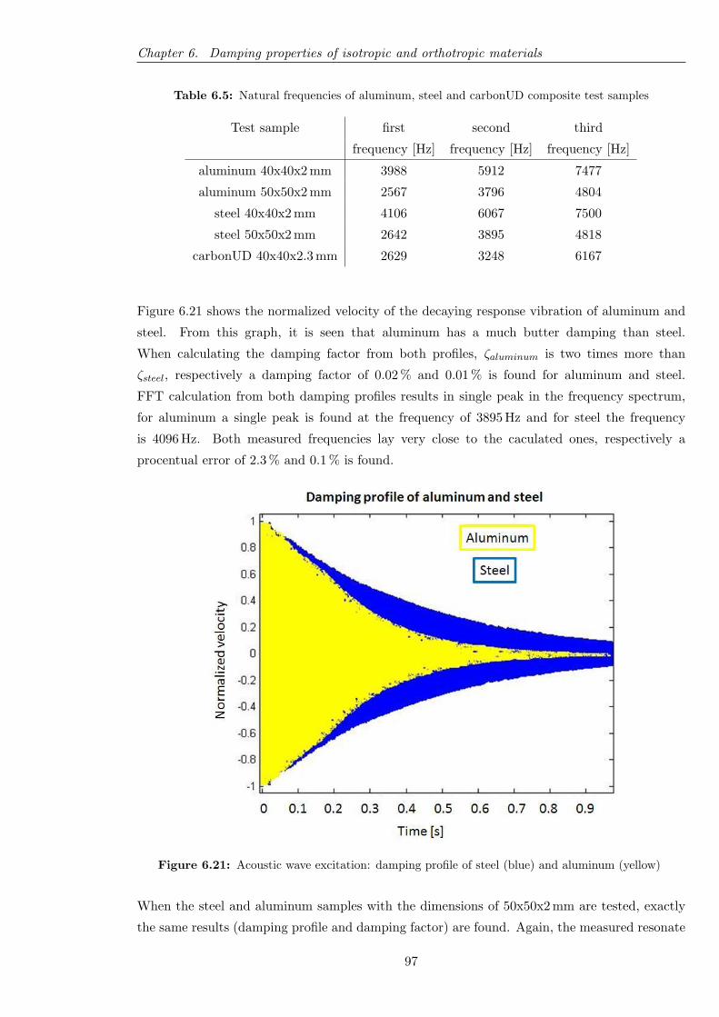
Chapter 6. Damping properties of isotropic and orthotropic materials
Table 6.5: Natural frequencies of aluminum, steel and carbonUD composite test samples
Test sample first second third
frequency [Hz] frequency [Hz] frequency [Hz]
aluminum 40x40x2 mm 3988 5912 7477
aluminum 50x50x2 mm 2567 3796 4804
steel 40x40x2 mm 4106 6067 7500
steel 50x50x2 mm 2642 3895 4818
carbonUD 40x40x2.3 mm 2629 3248 6167
Figure 6.21 shows the normalized velocity of the decaying response vibration of aluminum and
steel. From this graph, it is seen that aluminum has a much butter damping than steel.
When calculating the damping factor from both profiles, ζaluminum is two times more than
ζsteel, respectively a damping factor of 0.02 % and 0.01 % is found for aluminum and steel.
FFT calculation from both damping profiles results in single peak in the frequency spectrum,
for aluminum a single peak is found at the frequency of 3895 Hz and for steel the frequency
is 4096 Hz. Both measured frequencies lay very close to the caculated ones, respectively a
procentual error of 2.3 % and 0.1 % is found.
Figure 6.21: Acoustic wave excitation: damping profile of steel (blue) and aluminum (yellow)
When the steel and aluminum samples with the dimensions of 50x50x2 mm are tested, exactly
the same results (damping profile and damping factor) are found. Again, the measured resonate
97
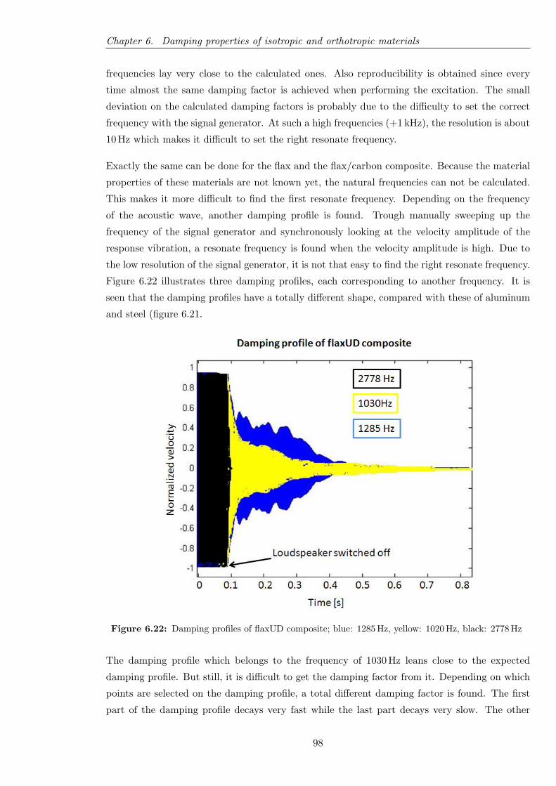
Chapter 6. Damping properties of isotropic and orthotropic materials
frequencies lay very close to the calculated ones. Also reproducibility is obtained since every
time almost the same damping factor is achieved when performing the excitation. The small
deviation on the calculated damping factors is probably due to the difficulty to set the correct
frequency with the signal generator. At such a high frequencies (+1 kHz), the resolution is about
10 Hz which makes it difficult to set the right resonate frequency.
Exactly the same can be done for the flax and the flax/carbon composite. Because the material
properties of these materials are not known yet, the natural frequencies can not be calculated.
This makes it more difficult to find the first resonate frequency. Depending on the frequency
of the acoustic wave, another damping profile is found. Trough manually sweeping up the
frequency of the signal generator and synchronously looking at the velocity amplitude of the
response vibration, a resonate frequency is found when the velocity amplitude is high. Due to
the low resolution of the signal generator, it is not that easy to find the right resonate frequency.
Figure 6.22 illustrates three damping profiles, each corresponding to another frequency. It is
seen that the damping profiles have a totally different shape, compared with these of aluminum
and steel (figure 6.21.
Figure 6.22: Damping profiles of flaxUD composite; blue: 1285 Hz, yellow: 1020 Hz, black: 2778 Hz
The damping profile which belongs to the frequency of 1030 Hz leans close to the expected
damping profile. But still, it is difficult to get the damping factor from it. Depending on which
points are selected on the damping profile, a total different damping factor is found. The first
part of the damping profile decays very fast while the last part decays very slow. The other
98
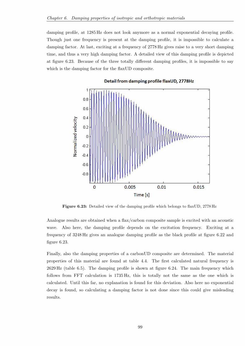
Chapter 6. Damping properties of isotropic and orthotropic materials
damping profile, at 1285 Hz does not look anymore as a normal exponential decaying profile.
Though just one frequency is present at the damping profile, it is impossible to calculate a
damping factor. At last, exciting at a frequency of 2778 Hz gives raise to a very short damping
time, and thus a very high damping factor. A detailed view of this damping profile is depicted
at figure 6.23. Because of the three totally different damping profiles, it is impossible to say
which is the damping factor for the flaxUD composite.
Figure 6.23: Detailed view of the damping profile which belongs to flaxUD, 2778 Hz
Analogue results are obtained when a flax/carbon composite sample is excited with an acoustic
wave. Also here, the damping profile depends on the excitation frequency. Exciting at a
frequency of 3248 Hz gives an analogue damping profile as the black profile at figure 6.22 and
figure 6.23.
Finally, also the damping properties of a carbonUD composite are determined. The material
properties of this material are found at table 4.4. The first calculated natural frequency is
2629 Hz (table 6.5). The damping profile is shown at figure 6.24. The main frequency which
follows from FFT calculation is 1735 Hz, this is totally not the same as the one which is
calculated. Until this far, no explanation is found for this deviation. Also here no exponential
decay is found, so calculating a damping factor is not done since this could give misleading
results.
99
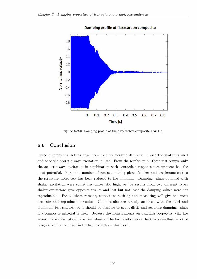
Chapter 6. Damping properties of isotropic and orthotropic materials
Figure 6.24: Damping profile of the flax/carbon composite 1735 Hz
6.6 Conclusion
Three different test setups have been used to measure damping. Twice the shaker is used
and once the acoustic wave excitation is used. From the results on all these test setups, only
the acoustic wave excitation in combination with contactless response measurement has the
most potential. Here, the number of contact making pieces (shaker and accelerometers) to
the structure under test has been reduced to the minimum. Damping values obtained with
shaker excitation were sometimes unrealistic high, or the results from two different types
shaker excitations gave opposite results and last but not least the damping values were not
reproducible. For all these reasons, contactless exciting and measuring will give the most
accurate and reproducible results. Good results are already achieved with the steel and
aluminum test samples, so it should be possible to get realistic and accurate damping values
if a composite material is used. Because the measurements on damping properties with the
acoustic wave excitation have been done at the last weeks before the thesis deadline, a lot of
progress will be achieved in further research on this topic.
100

Chapter 7
Conclusion
Within this master thesis, three main issues have been achieved. The first one is the literature
study on how to quantify the perception of the cyclist on comfort. Secondly the first steps in
frame optimization have been achieved. And at last, a promising test setup has been built to
measure material damping. From these three aspects, the main conclusion is given.
7.1 How to quantify the cyclist’s comfort
From literature study it is seen that comfort depends on many things. The perception of the
bicyclist on comfort is not due to one specific parameter. Many aspects have a distinct role
when comfort must be defined. One aspect is the frequency of the vibration coming from road
irregularities. From the ISO-2631 and IS0-5349 standard (respectively whole-body and hand-arm
vibration) it is clear that the frequency range up to 80 Hz is most important when evaluating
comfort. Another aspect is absorbed power, this describes the power loss of the rider due to
riding on a rough surface. Here, not only frequency but also the contact force between the rider
(hands, feet and seat) and the bicycle determine how many discomfort is felt by the rider. The
last method which is evaluated is through representing the frame as a SDOF spring-damper
system. The stiffness of the frame and mass of the cyclist are the main parameters which
define comfort. A low stiffness would result in more comfort, however this low stiffness is not
appreciated by the cyclist.
7.2 Frame optimization
Because optimization of a structure goes hand in hand with computer simulations, a numerical
computer model is made of the MF1 frame. This model gives the possibility to simulate how the
frame will react on external influences. In this topic of the research, it is possible to visualize
how the frame behaves (read: how it will deform) when it is subjected to an external force
with varying frequency. Not only computer simulations are important, but also experimental
verification is necessary. The dynamic properties of the frame are experimentally obtained by
means of Experimental Modal Analysis. From this test, the deformation of the frame can be
101
Chapter 7. Conclusion
visualized in the same way as it seen at the numerical simulation. When a good correlation
is achieved, the numerical model is correct and than it can be used for further optimizing.
The results from the lab experiments give different results than those seen at the computer
simulations, this is because not the right composite lay-up has been used on the numerical
model. If this should be the case, a match between both can be expected.
Another appreciable aspect on vibration testing is that the geometry of the structure plays a
distinct role when determining the dynamic properties of a structure. While measuring the
natural frequencies of a composite material (C-PPS 5 harness satin weave) it was seen that
the first measured and first calculated natural frequency did not match. An error of 36 % was
present. Better inspection of the plate led to the finding that some torsion was present at it.
Because also the first mode shape is a torsion mode, this has a major influence on the first
calculated frequency. Applying the correct torsion at the computer model of the composite
plate gives raise to a total different simulated first natural frequency. Finally, the error was only
3 %. From this experiment, it is clear that using the correct geometry for the computer model
is very important.
7.3 Test setup to measure damping
Many things on the bicycle can be changed to improve comfort, here the influence of the
bicycle frame material is investigated. Within this aspect, the material damping of different
materials has been assessed. Different kinds of test setups have been tried to establish a good
way of measuring material damping. From three different test setups, it is seen that only one
possibility is left. The test setup which uses contactless exciting and measuring response gives
the most accurate and reproducible results. This is done by means of acoustic wave excitation
and measuring response vibration is done with a laser vibrometer. From these experiments it
can be concluded that aluminum has a better material damping than steel. At this stage of the
research it is too early to decide whether or not the composite material based on flax fibre has
better damping than composite based on carbon fibre. Though, a lot of progress can be made
on this topic since it is still in its infancy.
7.4 Further research
Because some aspects at this master thesis are not finished yet, it is advised to keep on doing
research at this project. Based on the research which has been done in this master thesis, two
main aspects are put forward for further research. Firstly, the numerical frame model must
be updated with the correct composite lay-up. This makes it possible to correlate computer
simulations with experimental results. Secondly, the test setup to measure damping must be
improved, so it becomes possible to prove which material has the best damping properties and
thus has the most potential to use as a frame material and thus to improve comfort.
102

Chapter 7. Conclusion
Generally, the use of flax fibre as reinforcement material in load carrying applications has very
much potential. The use of flax fibre composite as a bicycle frame material is very interesting
to do research on it, especially when it makes part of the process in frame optimization.
103
Appendix A
Data sheets and drawings
Within this appendix, the calibration certificates, data sheets, drawings, etc. are summed below.
These can be found one after the other in the same order as enumerated below.
A.1 Accelerometers
1. Calibration certificate Kistler Accelerometer, type:8704B500, SN:2042793
2. Calibartion certificate PCB Accelerometer, type:352C64, SN:99055
3. Calibartion certificate PCB Accelerometer, type:352C64, SN:110062
A.2 Force sensor
4. Calibration certificate PCB force sensor, type:208C02, SN:29608
A.3 Data sheet shaker and Power Amplifier
5. Data sheet shaker LDSV406
6. Data sheet Power Amplifier PA100E-CE
A.4 2D Drawings MF1 and MF5 frame
7. 2D drawing MF1 frame: MF1-R839-540-L
8. 2D drawing MF5 frame: MF5-R839-540-S
A.5 Parts used for testing
9. Impact tip for impact hammer
10. Handgrip for impact hammer
104

Appendix A. Data sheets and drawings
11. Symmetric clamping system, part 1
12. Symmetric clamping system, part 2
13. Clamping system, part 1
14. Clamping system, part 2
105

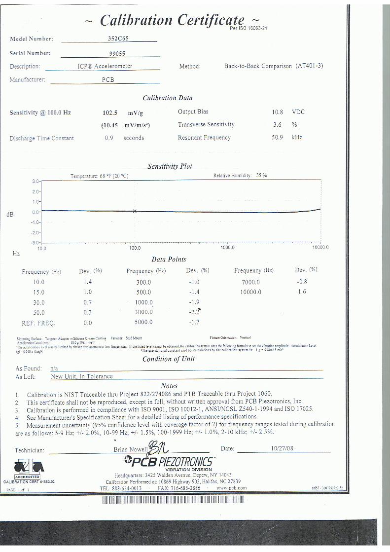


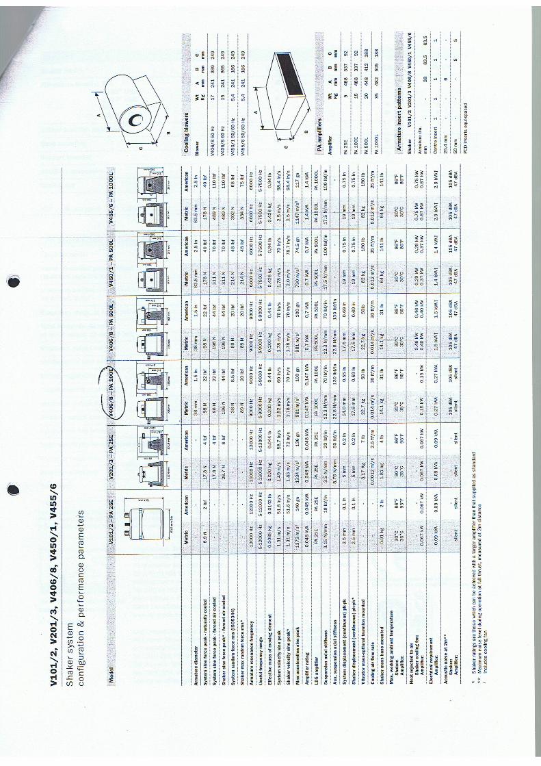

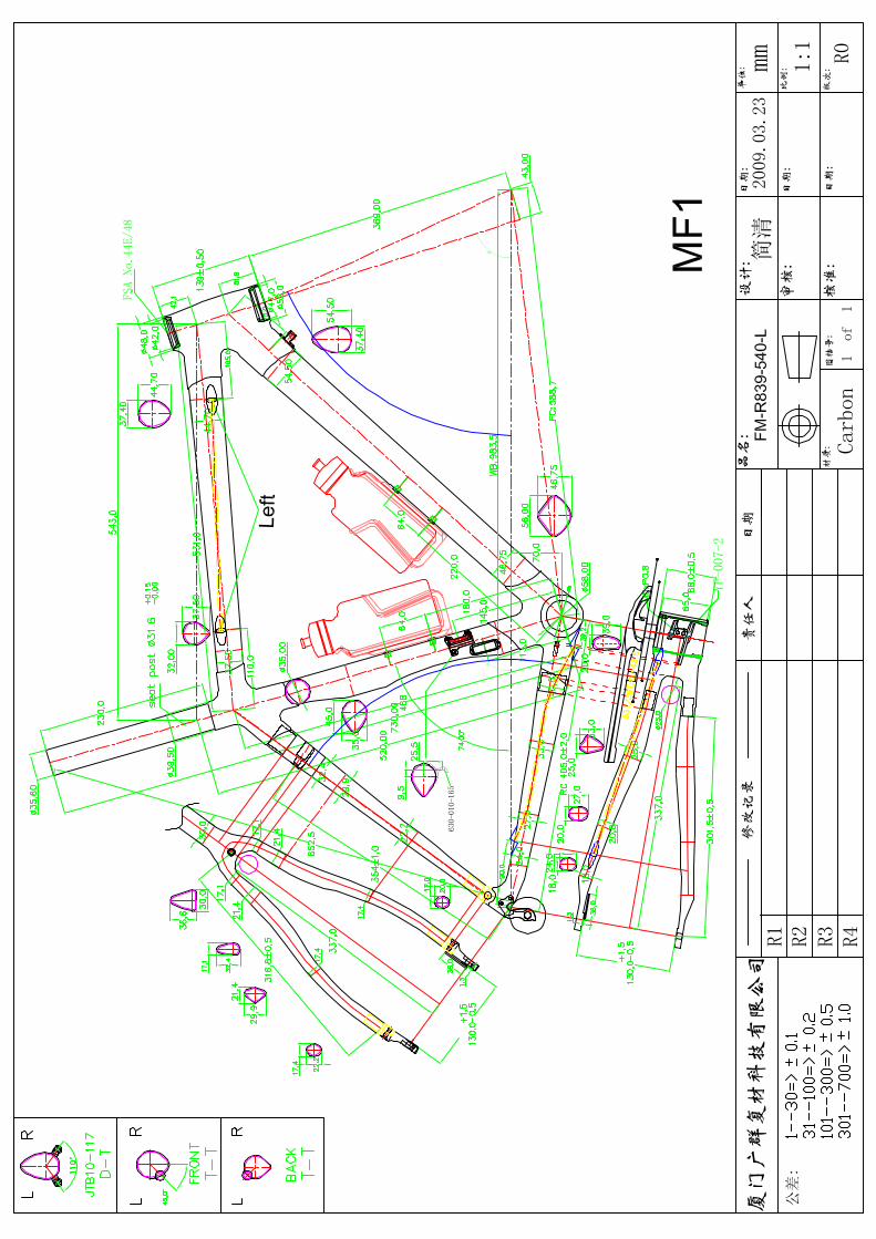
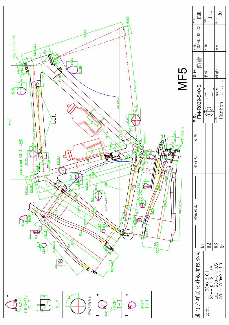
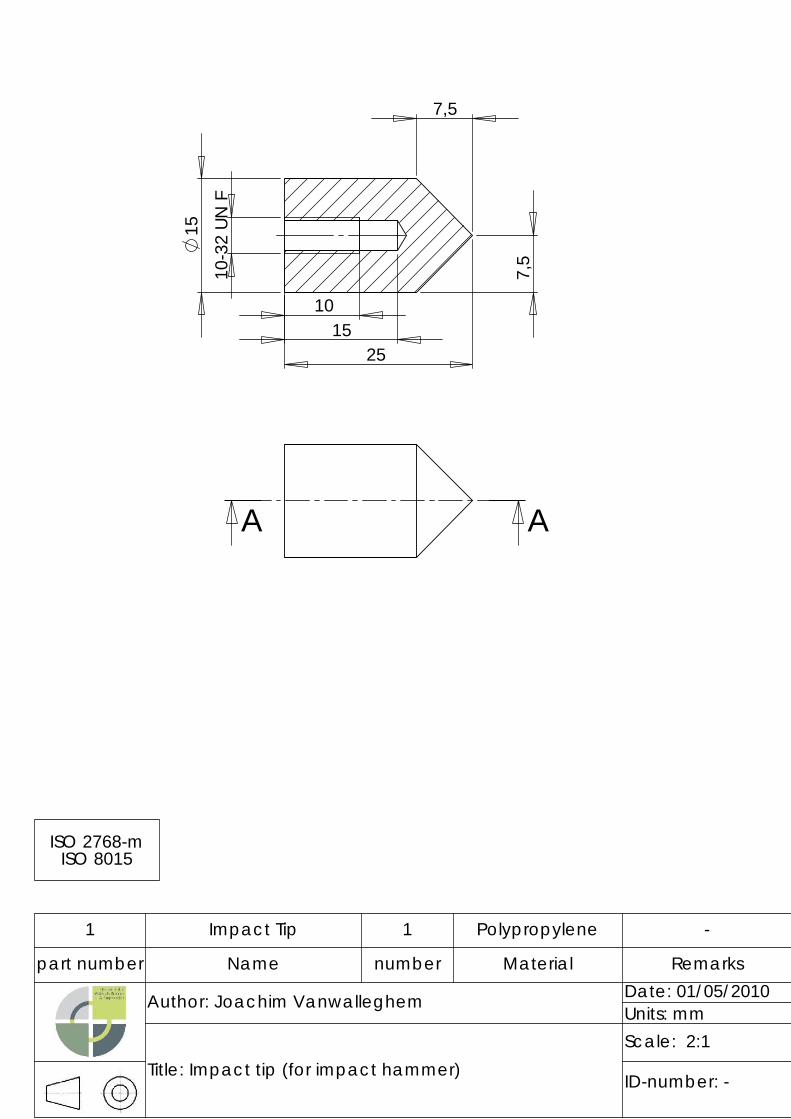
ID-number: -
Scale: 2:1
1 Impact Tip 1 Polypropylene -
part number Name number Material Remarks
Author: Joachim Vanwalleghem Date: 01/05/2010Units: mm
Title: Impact tip (for impact hammer)
ISO 2768-mISO 8015
A A
7,5
15
7,5
10-3
2 UN
F
1015
25

2510
Scale: 1:1
ID-number: -
1 Handgrip 1 Polypropylene -
part number Name number Material Remarks
Author: Joachim Vanwalleghem Date: 01/05/2010Units: mm
Title: Handgrip (for impact hammer)
ISO 2768-mISO 8015
20
6
130
M
20
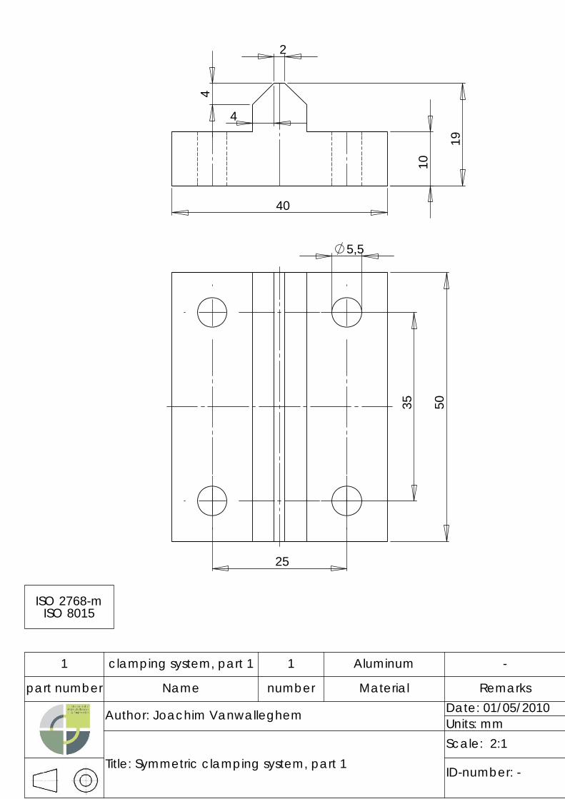
4
404
10
19
2
ID-number: -
Scale: 2:1
1 clamping system, part 1 1 Aluminum -
part number Name number Material Remarks
Author: Joachim Vanwalleghem Date: 01/05/2010Units: mm
Title: Symmetric clamping system, part 1
ISO 2768-mISO 8015
35
25
5,5
50
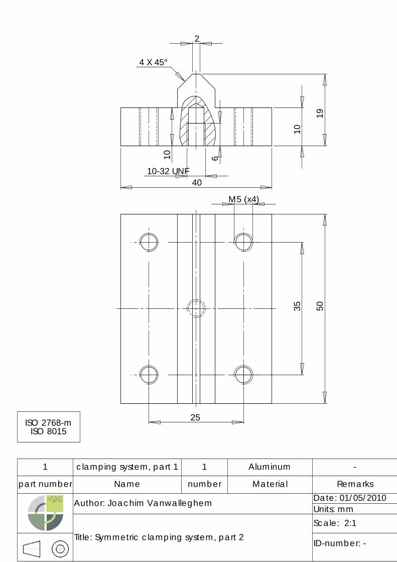
Scale: 2:1
ID-number: -
1 clamping system, part 1 1 Aluminum -
part number Name number Material Remarks
Author: Joachim Vanwalleghem Date: 01/05/2010Units: mm
Title: Symmetric clamping system, part 2
ISO 2768-mISO 8015
19
4
40
2
X 45°
10
10-32 UNF
610
35 50
M5 (x4)
25
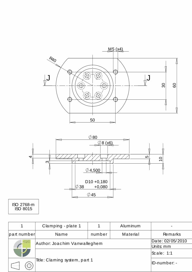
+
45
8 (x6)5
0,080
4,500
0,180
80
10
4
38D10
+
3
Scale: 1:1
ID-number: -
1 Clamping - plate 1 1 Aluminum -
part number Name number Material Remarks
Author: Joachim Vanwalleghem Date: 02/05/2010Units: mm
Title: Claming system, part 1
ISO 2768-mISO 8015
50
30 60
40R
M5 (x4)
J J
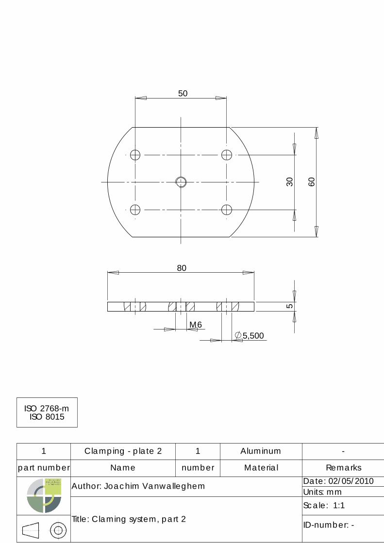
ID-number: -
Scale: 1:1
1 Clamping - plate 2 1 Aluminum -
part number Name number Material Remarks
Author: Joachim Vanwalleghem Date: 02/05/2010Units: mm
Title: Claming system, part 2
ISO 2768-mISO 8015
80
5,5006M
5
6030
50

Bibliography
[1] Joeri De Thaye. Determination of the static mechanical behaviour of flax-carbon raceframes.
Master’s thesis, Universiteit Gent, 2010.
[2] John Titlestad and et. al. Effect of suspension systems on the physiological and psychological
respones to sub-maximal biking on simulated smoothand bumpy tracks. Journal of Sports
Sciences, Febbruary:125–135, 2006.
[3] E. L. Wang and M. L. Hull. Minimization of pedaling induced energy losses in off-road
bicycle rear suspension systems. Vehicle system dynamics, October:291–306, 1997.
[4] Joris Degrieck. Composieten - mechanica van met vezels versterkte materialen. Universiteit
Gent, 1998.
[5] Edgars Sparnins. Mechanical properties of flas fibres and their composites. Master’s thesis,
Lulea, Sweden University of Technology, 2006.
[6] Mehmet Colakoglu. Damping and vibration analysis of polyethylene fiber composite under
varied temperature. 2006.
[7] M. Loccufier. Mechanische trillingen. Universiteit Gent, 2009.
[8] Mechanical vibration and shock - evaluation of human exposure to whole-body vibration –
part 1: General requirements, 1997.
[9] Mechanical vibration – measurement and evaluation of human exposure to
hand-transmitted vibration – part 1: General requirements.
[10] David Gordon Wilson. Bicycling science 3rd-ed. 2004.
[11] Y. Champoux, S. Richard, and J. M. Drouet. Bicycle structural dyanmics. Sound and
vibration, July:16–22, 2007.
[12] G. Beakaert. Composieten: technologie en productiemethoden. KHBO, 2009.
[13] Christel Cornelly. Algemene chemie - deel 1. KHBO, 2004.
[14] Joeri De Thaye. Autoclave manual for the production of flax UD and flax carbon test
specimen. Universiteit Gent, 2010.
120
Bibliography
[15] D. Arola, P. G. Reinhall, M. G. Jenkins, and S. C. Iverson. An experimental analysis of a
hybrid bicycle frame. Experimental Techniques, May/June:21–24, 1999.
[16] Craig Calfee and David Kelly. Bicycle frame materials comparison with a focus on carbon
fibre construction methods. Technical White Paper, October:1–13, 2002.
[17] n.a. Magnesium showcase. International magnesium association, 4:1–2, 2008.
[18] One nation magazine. Flavio deslandes eye-catching bamboo bicycles, December 2009.
[19] Billy Sperlich and et. al. Physiological and perceptual responses of adding vibration to
cycling. Journal of Exercise Physiology, 12:40–46, 2009.
[20] J. Rittweger, G. Beller, and D. Felsenberg. Acute physiological effects of exhaustive
whole-body vibration exercise in man. Clinical Phsiology, 20:134–142, 2000.
[21] Guide to good practice on hand-arm vibration.
[22] P. Lenzuni. Frequency and magnitude functional dependence of absorbed power resulting
from vibration transmitted to the hand and arm. Vibration Injury Network, May, 2001.
[23] R. Lundstrom, Holmlun P., and L. Lindberg. Absorption of energy during vertical
whole-body vibration exposure. Journal of biomechanics, 31:317–326, 1998.
[24] Menno Grootjans. Comfortabel presteren. Fiets, 02:18–25, 2010.
[25] n.a. Dossier koopwijzer. Grinta!, jan-feb:31–53, 2010.
[26] Peter Avitabile. Modal Space - In Our Own LIttle World. University of Massachusetta
Lowell, 2007.
[27] Simulia. Abaqus/CAE User’s Manual.
[28] Jeff Brown. Characterization of msc/nastran & msc/abaqus elements for turbine engine
blade frequency analysis. Turbine Engine Division, n.d.
[29] D. J. Ewins. Modal testing: Theory and Practice. Research Studies Press Ltd., 1984.
[30] Van Paepegem W. Degrieck J. Xu J. Lomov S.V. Daggumati, S. and I. Verpoest. Meso-scale
modelling in thermoplastic 5-harness satin weave composite. 17th International Conference
on Composite Materials (ICCM-17), 27-31 July 2009.
[31] Sumit Vasudeva, Rakesh K. Kapania, Eugene M. Cliff, and Pablo Tarazaga. Estimation
of elastic and damping characteristics of viscoelastically constrained carbon strands. In
Structures, Structural dynamics and Materials conference, 2006.
121