study of the viability of a glider drone for the return of ... · unmanned aerial vehicles (uav),...

Bachelor’s Degree in Aerospace Vehicle Engineering

Study of the viability of a glider drone for the return of

experiments carried by weather balloons

Report

Author:

Albert Gassol Baliarda

Director:

Manel Soria Guerrero

Co-Director:

Josep Oriol Lizandra Dalmases

June 12th, 2015

Contents

List of Figures iii

List of Tables v

1 Introduction 1

1.1 Aim of the project . . . . . . . . . . . . . . . . . . . . . . . . . . . . 1

1.2 Scope of the project . . . . . . . . . . . . . . . . . . . . . . . . . . . 1

1.3 Requirements . . . . . . . . . . . . . . . . . . . . . . . . . . . . . . . 2

1.4 Justification . . . . . . . . . . . . . . . . . . . . . . . . . . . . . . . . 2

2 State of the art 5

2.1 What are drones? . . . . . . . . . . . . . . . . . . . . . . . . . . . . . 5

2.1.1 Brief history of drones . . . . . . . . . . . . . . . . . . . . . . 5

2.2 Legal framework . . . . . . . . . . . . . . . . . . . . . . . . . . . . . 6

2.3 Gliders. An introduction . . . . . . . . . . . . . . . . . . . . . . . . . 6

2.3.1 Aerodynamic characteristics . . . . . . . . . . . . . . . . . . . 7

3 Approach and analysis of the main alternatives 9

3.1 Study of the atmospheric conditions . . . . . . . . . . . . . . . . . . 9

3.1.1 Earth’s atmosphere layers . . . . . . . . . . . . . . . . . . . . 9

3.1.2 Jet streams . . . . . . . . . . . . . . . . . . . . . . . . . . . . 10

3.2 Drone model selection . . . . . . . . . . . . . . . . . . . . . . . . . . 12

3.2.1 Main aerodynamic characteristics . . . . . . . . . . . . . . . . 12

3.2.2 Evaluation of existing models . . . . . . . . . . . . . . . . . . 13

3.2.3 Selection of the model . . . . . . . . . . . . . . . . . . . . . . 15

3.2.4 Discus 2b aerodynamic specifications . . . . . . . . . . . . . . 17

4 Development 21

4.1 Weather balloon launching . . . . . . . . . . . . . . . . . . . . . . . . 21

4.1.1 Balloon weight and calculation of the quantity of gas . . . . . 22

4.1.2 Trajectory calculation . . . . . . . . . . . . . . . . . . . . . . 27

4.2 Creation of a model . . . . . . . . . . . . . . . . . . . . . . . . . . . 29

4.2.1 Environment modelling . . . . . . . . . . . . . . . . . . . . . 29

Albert Gasssol Baliarda i

CONTENTS

4.2.2 Glider dynamics modelling . . . . . . . . . . . . . . . . . . . 33

4.3 The control system . . . . . . . . . . . . . . . . . . . . . . . . . . . . 45

4.3.1 Rolling control . . . . . . . . . . . . . . . . . . . . . . . . . . 51

4.3.2 Control of the angle of attack . . . . . . . . . . . . . . . . . . 57

4.4 Results . . . . . . . . . . . . . . . . . . . . . . . . . . . . . . . . . . . 61

5 Summary of results 65

5.1 Economic aspects . . . . . . . . . . . . . . . . . . . . . . . . . . . . . 65

5.2 Environmental study and implications . . . . . . . . . . . . . . . . . 67

5.2.1 Drone environmental issues . . . . . . . . . . . . . . . . . . . 67

5.2.2 Environmental wastes . . . . . . . . . . . . . . . . . . . . . . 67

5.3 Security aspects . . . . . . . . . . . . . . . . . . . . . . . . . . . . . . 68

5.3.1 Weather balloon-related security aspects . . . . . . . . . . . . 68

5.3.2 Drone-related security aspects . . . . . . . . . . . . . . . . . . 68

5.4 Temporal aspects and planning . . . . . . . . . . . . . . . . . . . . . 69

5.4.1 List of tasks . . . . . . . . . . . . . . . . . . . . . . . . . . . . 69

5.5 Conclusions and recommendations . . . . . . . . . . . . . . . . . . . 70

Bibliography 73

ii Albert Gasssol Baliarda

List of Figures

2.1 MQ-9 Reaper drone . . . . . . . . . . . . . . . . . . . . . . . . . . . 6

2.2 ASW 28, a modern glider built by the German Alexander Schleicher 7

2.3 ASW 28 polar curve . . . . . . . . . . . . . . . . . . . . . . . . . . . 8

3.1 Temperature variation throughout the altitude . . . . . . . . . . . . 10

3.2 Earth representation with the polar and subtropical jets’ location . . 11

3.3 Scheme of the forces acting on a rectilinear, symmetric and non-

accelerated gliding . . . . . . . . . . . . . . . . . . . . . . . . . . . . 13

3.4 Discus 2b 1:3.75 scale model from Icare RC . . . . . . . . . . . . . . 15

3.5 Real Discus 2b 3-side view . . . . . . . . . . . . . . . . . . . . . . . . 16

3.6 Airfoil HQ 2.5/12 shape . . . . . . . . . . . . . . . . . . . . . . . . . 17

3.7 Airfoil HQ 2.5/12 aerodynamic polar . . . . . . . . . . . . . . . . . . 17

3.8 Airfoil HQ 2.5/12 Cl−alpha graph . . . . . . . . . . . . . . . . . . . 18

3.9 Discus 2b polar curve in a range of velocities from 12 m/s to 80 m/s 19

3.10 Plot of the glide ratio against the horizontal velocity . . . . . . . . . 19

4.1 Scheme of the forces acting in a body immersed in the air . . . . . . 22

4.2 Dependency of the drag coefficient of a sphere and the Reynolds number 23

4.3 Plots of the altitude and the ascent rate of the balloon and its payload 27

4.4 Interface of the habhub trajectory predictor . . . . . . . . . . . . . . 28

4.5 Simulation of the trajectory of the balloon . . . . . . . . . . . . . . . 29

4.6 Wind profile with its quadratic wind gradient, blowing easterwards . 31

4.7 Evolution of the altitude and the dive velocity starting at h = 20000 m

with v = 0 . . . . . . . . . . . . . . . . . . . . . . . . . . . . . . . . . 38

4.8 Sequence of the drone’s gliding start . . . . . . . . . . . . . . . . . . 45

4.9 Trajectory of the drone in the firsts 10 minutes, flying without rolling 45

4.10 Scheme about the integration process and how the control system works 46

4.11 Top view of the drone with an arbitrary position and orientation with

the values of angReal and angSmall in each zone . . . . . . . . . . . 53

4.12 Example of a standard path generated by pathGen . . . . . . . . . . 56

4.13 Phugoid oscillation as a result of a too much abrupt change of CL . 58

4.14 Smooth transition from the nose diving to a normal gliding attitude 58

Albert Gasssol Baliarda iii

LIST OF FIGURES

4.15 3D plot of the whole trajectory followed by the drone . . . . . . . . 61

4.16 Altitude variation with time . . . . . . . . . . . . . . . . . . . . . . . 62

4.17 Air-relative flight path angle variation with time . . . . . . . . . . . 62

4.18 Horizontal distance from the landing location at each moment . . . . 63

4.19 Variation of the aerodynamic velocity with time . . . . . . . . . . . . 63

iv Albert Gasssol Baliarda

List of Tables

3.1 Reference aerodynamic parameters of glider aircraft . . . . . . . . . 12

3.2 List of scale models with span major than 4 m and its main specifi-

cations based on the Icare – Sailplanes and Electrics catalogue . . . 14

3.3 Discus 2b scale model specifications . . . . . . . . . . . . . . . . . . 15

4.1 Summary of the results of the balloon ascent . . . . . . . . . . . . . 27

4.2 Configuration of the parameters with which has been ran the trajec-

tory simulation . . . . . . . . . . . . . . . . . . . . . . . . . . . . . . 28

4.3 Main parameters that are used by the control system . . . . . . . . . 51

5.1 List of products with its unit prices . . . . . . . . . . . . . . . . . . . 66

5.2 Exchange rate used in this budget . . . . . . . . . . . . . . . . . . . 66

5.3 Budget of the project . . . . . . . . . . . . . . . . . . . . . . . . . . 66

Albert Gasssol Baliarda v

Chapter 1

Introduction

1.1 Aim of the project

The aim of this project is to study the technical viability of a glider drone capable

of taking back a determined experiment or payload from the stratosphere, leaving

from a non-recoverable weather balloon. The drone must be able to glide through

the different layers of the atmosphere to go back to the base or any of the pre-

programmed “way-points” in an autonomous way and without any kind of propulsion

system.

1.2 Scope of the project

In this project it will be encompassed the following tasks:

� Justification of the project. A study about the state of the art of the drones’

field will be done. This study will permit to define the possible applications of

the project, or maybe redefine it a little.

� Study of the requirements for the drone operational conditions. The drone is

thought to glider starting from the stratosphere, so it will have to be considered

the conditions at which the drone will operate to carry out its mission. These

conditions will fix a set of requirements that the drone will have to satisfy.

� Selection of the drone model. Taking into account the previous study, it will

be done a market research in order to select the drone model that best fits the

requirements criteria. Afterwards, it will have to be obtained or estimated all

the aerodynamic data needed to develop the next stages.

� Development of a physical model. The dynamics of the drone gliding perfor-

mances and the environment characterisation will be modelled with a physical

model in order to simulate and analyse the drone response.

Albert Gasssol Baliarda 1

1. INTRODUCTION

� Verification of the physical model. After developing a preliminary physical

model, it will be carried out different tests to check if it has been correctly

developed and the drone response is as expected.

� Establishment of a 3D control system. Once the model has been verified, the

3D control system will be established. For this, it will be considered all the

situations that the drone could encounter during the flight and which must be

the response to these ones.

� Study of the viability of the project. At the end, the project will be summarized

and it will be listed possible aspects to improve. If there are any costs, these

will be estimated in a budget. There must exist a conclusion that, based on

the results of this study, rules if the project can really be achievable or not.

1.3 Requirements

The characteristics of this project do not fix, or do not make necessary to fix, any

set of technical requirements which it must compulsorily accomplish (e.g. gliding at

a determined speed, measuring a determined dimensions. . . ). It is a study about the

technical viability to operate or not at the conditions described in Section 1.1.

Therefore, the imposed requirements are basically the ones that would allow to

accomplish the objectives previously described, this is:

� Ability to reach an altitude of 20 km.

� Absence of any kind of propulsion system.

� Ability to return in an autonomous way to the desired point.

1.4 Justification

In the last years, drones have acquired a significant importance for carrying out a

determined kind of tasks in the civilian sphere. This trend is mainly due to two

reasons. On the one hand, the usage of drones avoids to put at risk the pilot’s life

in situations that can turn out dangerous, such as flying over irregular and difficult-

to-reach areas or natural disasters. On the other hand, the usage of drones instead

of a manned airplane or helicopter, e.g. for aerial filming or security surveillance,

represents a significant reduction of the mission costs.

The replacement of manned aerial vehicles with drones has been done mainly to

roles which are dull, dirty or dangerous [1]. Thus, some of the uses to which drones

may be are:

� Aerial photography – Film, video, still, etc.

2 Albert Gasssol Baliarda

� Agriculture – Crop monitoring and spraying; herd monitoring and driving.

� Coastguard – Search and rescue, coastline and sea-lane monitoring.

� Conservation – Pollution and land monitoring.

� Costums and excise – Surveillance for illegal imports.

� Electricity companies – Powerline inspection.

� Fire services and Forestry – Fire detection, incident control.

� Fisheries – Fisheries protection.

� Gas and oil supply companies – Land survey and pipeline security.

� Information services – News information and pictures, feature pictures, e.g.

wildlife.

� Lifeboat Institutions – Incident investigation, guidance and control.

� Local Authorities – Survey, disaster control.

� Meteorological services – Sampling and analysis of atmosphere for forecasting,

etc.

� Traffic agencies – Monitoring and control of road traffic.

� Oil companies – Pipeline security.

� Ordnance Survey – Aerial photography for mapping.

� Police Authorities – Search for missing persons, security and incident surveil-

lance.

� Rivers Authorities – Water course and level monitoring, flood and pollution

control.

� Survey organisations – Geographical, geological and archaeological survey.

� Water Boards – Reservoir and pipeline monitoring.

So, there are lots of applications which drones may be useful for. Some of them

require an accurate and continuous flight, and the need of an engine or batteries

on board is obvious to give the drone the necessary power to fly and carry out its

mission.

However, there are also some applications to which it is only necessary to overfly

a determined area, and not hovering over this area during a certain amount of time

observing or doing something else. For this second sort of applications, the absence

of the heavy batteries in charge of providing the propulsion forces on the drone


1. INTRODUCTION

would mean a saving in its weight, as well as a reduction of costs, as much the

design and fabrication costs as the operation and maintenance ones. The weight

corresponding to these batteries, as well as the physical space they would take out

inside the drone, could be better employed carrying a more heavy or bulky payload,

and so the applications range of the drone would be extended.

In this way, the concept of a glider drone, capable of carrying out a determined

mission leaving from a high altitude at which has ascended by means of a weather

balloon, and capable of returning to a determined point in an autonomous way and

without any propulsion system, results a very interesting idea to develop and study

if it could really be possible to implement.


Chapter 2

State of the art

2.1 What are drones?

Unmanned aerial vehicles (UAV), commonly known as drones, are aircraft without

any human pilot aboard. The International Civil Aviation Organization (ICAO)

classifies unmanned aircraft into two types under Circular 328 AN/190 :1

� Autonomous aircraft – currently considered unsuitable for regulation due to

legal and liability issues.

� Remotely piloted aircraft – subject to civil regulation under ICAO and under

the relevant national aviation authority.

The ICAO also refers to this second sort of drones as RPA (remotely piloted

aircraft), and calls UAS (unmanned aircraft systems) to the whole system that

comprises the ensemble of subsystems, such as the control station, support and

communication subsystems and the aircraft itself. However, this last concept refers

to military technologies and sophisticated intelligent systems rather than the smaller

and more commonly used drones for civilian applications, to which it is not needed

such complexity.

2.1.1 Brief history of drones

First UAV appeared in the mid-19th century, when the Austrian army used un-

manned balloons to bomb Venice [3]. Since then, drones have been constantly in

development, always in the military field, so they have been identified as war means

by the society. Nowadays, more than 60 countries are developing programs to include

UAS technologies to their armies [4].

Drones began being employed in supervision, surveillance and exploration mis-

sions. Later on, it began to be built drones capable of being equipped with attack

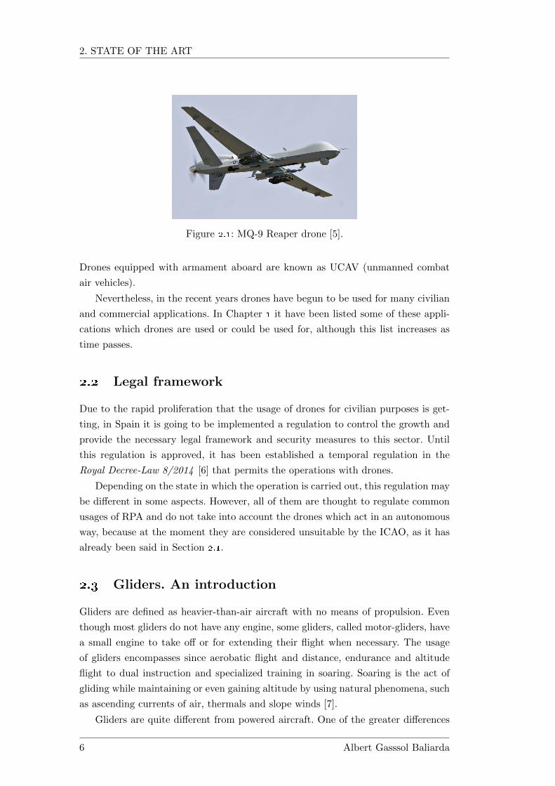
armament, such as the MQ-9 Reaper drone built by General Atomics (Figure 2.1).

1Circular 328 AN/190 from ICAO can be seen in [2].


2. STATE OF THE ART

Figure 2.1: MQ-9 Reaper drone [5].

Drones equipped with armament aboard are known as UCAV (unmanned combat

air vehicles).

Nevertheless, in the recent years drones have begun to be used for many civilian

and commercial applications. In Chapter 1 it have been listed some of these appli-

cations which drones are used or could be used for, although this list increases as

time passes.

2.2 Legal framework

Due to the rapid proliferation that the usage of drones for civilian purposes is get-

ting, in Spain it is going to be implemented a regulation to control the growth and

provide the necessary legal framework and security measures to this sector. Until

this regulation is approved, it has been established a temporal regulation in the

Royal Decree-Law 8/2014 [6] that permits the operations with drones.

Depending on the state in which the operation is carried out, this regulation may

be different in some aspects. However, all of them are thought to regulate common

usages of RPA and do not take into account the drones which act in an autonomous

way, because at the moment they are considered unsuitable by the ICAO, as it has

already been said in Section 2.1.

2.3 Gliders. An introduction

Gliders are defined as heavier-than-air aircraft with no means of propulsion. Even

though most gliders do not have any engine, some gliders, called motor-gliders, have

a small engine to take off or for extending their flight when necessary. The usage

of gliders encompasses since aerobatic flight and distance, endurance and altitude

flight to dual instruction and specialized training in soaring. Soaring is the act of

gliding while maintaining or even gaining altitude by using natural phenomena, such

as ascending currents of air, thermals and slope winds [7].

Gliders are quite different from powered aircraft. One of the greater differences


is a completely different arrangement of the landing gear as a result of the light

weight of the aircraft and the absence of a propeller. Others are that the pilot’s

seat is located toward the front so that the centre of gravity will fall within 25 –

30% of the mean aerodynamic chord of the wing forward, the wing span is always

considerable, and the fuselage and other components are well streamlined to obtain

the maximum aerodynamic efficiency, which has a lot of importance on gliders. An

example of all of this can be seen in Figure 2.2.

Figure 2.2: ASW 28, a fifteen meter span modern glider built by the German Alexan-der Schleicher. Extracted from http://www.alexander-schleicher.de/.

2.3.1 Aerodynamic characteristics

The most important parameters that define a glider flight are the glide ratio and the

sink rate. The glide ratio, also called efficiency, is the ratio between the horizontal

travelled distance and the loss of altitude. It can be expressed as an efficiency value,

e.g. 20, or as a ratio, 20:1, and is an indication of the quality of a glider. The sink

rate is the amount of altitude lost by the glider in a unit of time in relation with

the surrounding air. It is commonly expressed in meters per second.

The graph that best describes the glider performances then is the polar curve.

The polar curve contrasts the sink rate of the aircraft with its horizontal speed, and

gives the glide ratio in each case (see Figure 2.3). From the polar curve, it is possible

to know the best glide ratio that a glider can achieve, and the situation at which it

occurs as well. The best glide ratio is obtained when the ratio between horizontal

speed and sink rate is maximum, so, as it can be seen in the ASW 28 polar curve

shown in Figure 2.3, it is found in the tangent point between the curve and a straight

line from the origin [8].


http://www.alexander-schleicher.de/

2. STATE OF THE ART

Figure 2.3: ASW 28 polar curve. Extracted from http://www.

alexander-schleicher.de/.




Chapter 3

Approach and analysis of the

main alternatives

3.1 Study of the atmospheric conditions

In this section it will be studied the characteristics of the atmosphere –concretely,

of the layers at which the drone will operate –in order to obtain the conditions and

requirements that it imposes. For this, it will always be considered the International

Standard Atmosphere (ISA) model (see Appendix A).

3.1.1 Earth’s atmosphere layers

The Earth’s atmosphere is divided in several layers, each one having its own prop-

erties. These layers are the troposphere, stratosphere, mesosphere, thermosphere

and exosphere. In the present project, it will be dealt with the troposphere and

stratosphere, and its main characteristics are described below [9].

Troposphere

The troposphere is the lowest layer of the Earth’s atmosphere. It is characterised for

the most part by decreasing temperature with height approximately at a constant

rate (see Figure 3.1). It contains about 80% of the total atmospheric mass. The

troposphere is the most influenced layer by the energy transfer that takes place

at the Earth’s surface through evaporation and heat conduction. These processes

create horizontal and vertical temperature gradients which lead to the development

of atmospheric motions and the upward transport of heat and water vapour.

The vertical extent of the troposphere varies with season and latitude. In tropical

regions it is usually 16 − 18 km. Over the poles the extent in summer is about

8− 10 km, but in the winter the troposphere may be entirely absent.

The troposphere is bounded at the top by a remarkably abrupt increase of static

stability with height, this means, temperature stops decreasing with height. The


3. APPROACH AND ANALYSIS OF THE MAIN ALTERNATIVES

Figure 3.1: Temperature variation throughout the altitude [9].

surface formed by this discontinuity of lapse rate is called the tropopause.

Stratosphere

The stratosphere is the statically stable layer above the troposphere. It extends

upward to a height of about 50 km, where the temperature is comparable to the

Earth’s surface temperature (see Figure 3.1). Above the tropopause the temperature

first hardly increases, but to about 20 km it starts to increase rapidly.

This temperature distribution is associated with the absorption of ultraviolet

solar radiation by the ozone, which is present between the heights of 20 and 50 km.

These radiation processes, in combination with intensive dynamical and chemical

processes, make the stratosphere to be a region in which the horizontal mixing of

gases is much more important and proceeds much more rapidly than the vertical

mixing.

The top of the stratosphere is a surface of maximum temperature called stratopause,

which separates the stratosphere and the next atmospheric layer, the mesosphere.

3.1.2 Jet streams

Jet streams are narrow fast flowing air currents located at altitudes around the

tropopause [10]. The World Meteorological Organization (WMO) defines them as

“strong and narrow air streams concentrated along a nearly horizontal axis in the

high troposphere and the stratosphere, characterized by a strong horizontal and

vertical wind shear. Presenting one or two velocity peaks, jet streams flow throughout

several thousands of kilometres on strips of various hundreds of kilometres of width


and various kilometres of thickness”.

Jet streams are West to East winds, which can stop, split, combine into one

stream and flow in various directions. There exist four jet streams, two in each

hemisphere (Figure 3.2):

� Polar jets. They are the strongest jet streams and are located at around

7−12 km of altitude, where the pressure level is around 25 kPa (250 mbar). The

northern hemisphere polar jet is found between latitudes 50° N and 60° N [11]

and usually reach speeds greater than 100 km/h, although velocity peaks

within the jet are much higher (it have been measured speeds over 400 km/h).

� Subtropical jets. They are weaker than polar jets, and are located at much

higher altitudes than them, around 10 − 16 km. The northern hemisphere

subtropical jet is usually found at latitudes around 30° N.

Both polar and subtropical jet streams are displaced poleward in summer and equa-

torward in winter.

Figure 3.2: Earth representation with the polar and subtropical jets’ location [11].

Jet streams analysis

Due to the aim of this project, it is of primordial importance to have a relative

detailed knowledge about the behaviour of these high speed winds. Europe, and

therefore Spain, are directly affected by the northern polar jet, so it will have a

direct effect on the drone specifications.

In this way, it has been carried out a statistical study about the polar jet intensity

above the Spanish territory during the year previous to this study, which can be seen

in detail in Appendix B. It concludes that, even though sometimes intensive wind

speeds up to 150 kt are detected, it is not usual. Jet stream speeds do not usually

exceed of 60 kt, and when they do, they rarely go over 70 kt (about the 18% of the

days).

According to these results, and being impossible to deal with the highest wind

speeds, it is necessary to take a trade-off. Thus, it will be considered that the max-

imum jet stream speeds are of 70 kt, this is, the drone is requested to be capable to



fly with wind speeds of this intensity; or in other words, it will not be designed to

fly when wind speeds are major than 70 kt.

3.2 Drone model selection

On the basis of what has been established so far, it has to be chosen an existing

drone model that fits to the operational requirements. It is important to point out

that, due to this is a preliminary design project, the chosen model might not be

the same that which would be chosen if this project was continued and some other

detailed design phases would be dealt with. Actually, in such case the best option

would be to design a new drone specifically for this mission.

Whatever the case may be, this is out of the scope of this project. It has to be

chosen a drone model already existing which can be considered appropriate for this

kind of mission and work upon this basis.

3.2.1 Main aerodynamic characteristics

As a starting point, and taking it as general data, one can consider the basic aero-

dynamic parameters of glider aircraft to be close to what Table 3.1 shows [12].

Parameter Symbol Value

Aspect ratio Λ 15 – 20Zero-lift drag coefficient CD0 0,012Efficiency factor ϕ 0,9

Table 3.1: Reference aerodynamic parameters of glider aircraft.

With these data it is possible to calculate a general value of the induced drag

parameter K and have an idea of its order of magnitude for a glider:

K =1

πΛϕ(3.1)

K = 0.02

If one sets out the general equations for rectilinear, symmetric and non-accelerated

gliding (see Figure 3.3) it results:

W cos γ − L = 0 (3.2)

W sin γ −D = 0 (3.3)

And considering a small glide angle (γ � 1), developing (3.2) gives the following:

W − 1

2ρv2SwCL = 0


Figure 3.3: Scheme of the forces acting on a rectilinear, symmetric and non-accelerated gliding.

v =

√2

ρCL

W

Sw(3.4)

Equation (3.4) shows that the higher is the aerodynamic velocity, the higher must

be the wing loading. In the present case, it is necessary to have the capability to fly

at high aerodynamic velocities in order to exceed the strong wind speeds previously

analysed, especially when the drone flies with headwind. Thus, a high wing loading

is a basic and important requirement to satisfy.

3.2.2 Evaluation of existing models

Taking into account the requirement of high wing loading, it has been done a research

of the glider scale models that currently exist. Scale models are generally built

of lightweight materials like plastics and foams, so the great majority of common

scale models present low wing loadings. However, looking for models built in a little

major scales and with a little major complexity, the specifications are closer to the

requested.

Table 3.2 contains a list of scale gliders based on the Icare – Sailplanes and

Electrics catalogue [13] with its specifications, as well as the added field of the

induced drag parameter K according to Table 3.1 data and Equation (3.1).



ModelSpan(m)

Wingarea (m2)

Weight(kg)

Wing load.(kg/m2)

Λ K

ASW-28 4 0,68 5,4 7,94 23,53 0,016H-201 Standard Libelle 4,02 0,695 4,8 6,91 23,25 0,016L23-Super Blanik 4,05 1,2 8,5 7,08 13,67 0,027Salto H101 4,06 0,7 6 8,57 23,55 0,016ASH-26 4,05 - 5,8 - - -Moswey 4 3,9 1,02 5 4,90 14,91 0,025Cirrus 4,5 0,81 6 7,41 25,00 0,015DG-800S/M 4,2 0,63 3,5 5,56 28,00 0,013L213 A 4,63 1,211 12 9,91 17,70 0,021DG-800S 3,75 0,713 5 7,01 19,72 0,019SB-9 4,5 0,583 4,4 7,55 34,73 0,011Ventus 2cx 4,3 0,71 5,3 7,46 26,04 0,014Salto H101 (2) 4,5 0,72 5,5 7,64 28,13 0,013ASG 29-18 4,8 0,877 5,6 6,39 26,27 0,014DG-600M 4 0,75 5 6,67 21,33 0,018Ka6e 4,2 0,91 6,6 7,25 19,38 0,019DG-1000/M 4,8 1,12 12 10,71 20,57 0,018ASK-21 4,2 0,94 6,3 6,70 18,77 0,020Discus 2b/2bM 4 0,71 5,7 8,03 22,54 0,017Nimbus 4 6 0,8 7,5 9,38 45,00 0,008Discus 2b (2) 4 0,653 6,8 10,41 24,50 0,015ASH-26 (2) 6 - 11,5 - - -Discus 4,3 0,87 5,7 6,55 21,25 0,018DG-600 5 1,12 9,5 8,48 22,32 0,017SB-15 5,14 0,885 6,5 7,34 29,85 0,013ASG 29 5 0,877 7,5 8,55 28,51 0,013Pilatus B4 4,5 1,275 9,5 7,45 15,88 0,024DFS-Habicht 3,89 1,3 - - 11,64 0,032DFS-Reiher 5,4 1,65 9,35 5,67 17,67 0,021Ventus 2ax 5 1,05 8 7,62 23,81 0,016Lunak LF-107 4,75 1,43 15 10,49 15,78 0,024DG-600/16 Evo 5,13 0,95 6,5 6,84 27,70 0,014Duo DiscusX 5,33 1,09 10,5 9,63 26,06 0,014ASW-22 BL 5,3 0,68 5 7,35 41,31 0,009Ventus 2cx (2) 5 1,25 11,5 9,20 20,00 0,019HpH 304 Shark 6 1,33 13 9,77 27,07 0,014ASG 29 6 1,2 11 9,17 30,00 0,012ASK-21 (2) 6 2,35 19 8,09 15,32 0,024Swift S-1 5,5 1,56 18 11,54 19,39 0,019Arcus 6,6 1,74 20 11,49 25,03 0,015Nimbus 4D/DM 7,06 1,29 13 10,08 38,64 0,010

Table 3.2: List of scale models with span major than 4 m and its main specificationsbased on the Icare – Sailplanes and Electrics catalogue.


3.2.3 Selection of the model

As it has already been said, the main requirement that the chosen drone must satisfy

is a high wing loading. However, there are some other factors which are important

too, for instance the aspect ratio and, hence, the span. The more is the aspect ratio,

the more is the aerodynamic efficiency of an airplane, fact that results of primordial

importance in a glider. The weight is important too, since even though a major

weight directly implies a major wing loading, it must not be forgotten that the

glider shall be raised at 20000 m by means of a weather balloon, and a heavy weight

means more difficulties and, in general, a higher cost of the operation.

In this way, the 1:3.75 scale model Discus 2b results a great and equilibrated one.

Figure 3.4 shows the glider model, and its specifications are summarized in Table 3.3

(some of which are repeated in Table 3.2).

Parameter Value Units

Span 4 mLength 1,85 mWing area 0,653 m2

Weight 6,8 kgWing loading 10,41 kg/m2

Aspect ratio 24,5 -Wing airfoil HQ 2.5/12 -

Table 3.3: Discus 2b scale model specifications.

It presents a high wing loading but not an excessive heavy weight, which obvi-

ously is due to a lower wing area, as well as a good aspect ratio within the usual

values. The induced drag parameter results K = 0.015, which is a quite low value.

As it has already been said, this drone model is taken as a reference to work

in during this preliminary study, and its design and specifications should not be

considered as definitives if more advanced design phases of the project will be dealt

with.

Figure 3.4: Discus 2b 1:3.75 scale model from Icare RC [13].


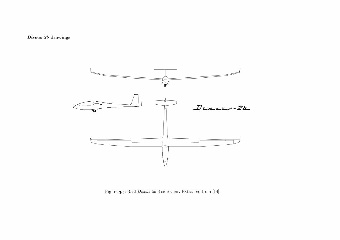
Discus 2b drawings

Figure 3.5: Real Discus 2b 3-side view. Extracted from [14].

3.2.4 Discus 2b aerodynamic specifications

Airfoil curves

The chosen Discus 2b scale model uses the wing airfoil HQ 2.5/12. It is an aero-

dynamic airfoil widely used in radio control scale gliders and sailplanes, which co-

ordinates can be found in [15]. It presents a maximum thickness of 12% at 35% of

chord, and a maximum camber of 2.5% at 50% of chord. Figure 3.6 represents the

shape of this aerodynamic airfoil.

Figure 3.6: Airfoil HQ 2.5/12 shape [15].

The website www.airfoiltools.com provides the aerodynamic polar of the air-

foil and the plot of the airfoil Cl against the angle of attack, amongst other useful

data. All these data have been obtained with XFoil1 simulations, at several Reynolds

numbers. Technical details about the running of these simulations are available at

the airfoiltools webpage. Figure 3.7 and Figure 3.8 are the HQ 2.5/12 aerodynamic

polar and Cl − α graph, respectively. Both graphs correspond at Re = 500000,

which is a representative value of the average air flow characteristics at which the

drone will fly. The data in which these graphs are based can be found tabulated in

Appendix C.

Figure 3.7: Airfoil HQ 2.5/12 aerodynamic polar.

The linear part of the Cl−α graph between Clmin = −0.6799 and Clmax = 1.3331

1An interactive program for the design and analysis of subsonic isolated airfoils created by MarkDrela at MIT.


www.airfoiltools.com


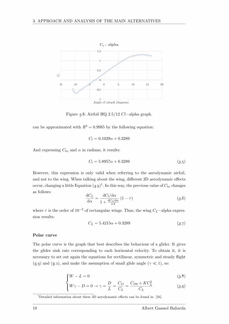
Figure 3.8: Airfoil HQ 2.5/12 Cl−alpha graph.

can be approximated with R2 = 0.9985 by the following equation:

Cl = 0.1029α+ 0.3289

And expressing Clα and α in radians, it results:

Cl = 5.8957α+ 0.3289 (3.5)

However, this expression is only valid when referring to the aerodynamic airfoil,

and not to the wing. When talking about the wing, different 3D aerodynamic effects

occur, changing a little Equation (3.5)1. In this way, the previous value of Clα changes

as follows:dCLdα

=dCl/dα

1 + dCl/dαπΛ

(1− τ) (3.6)

where τ is the order of 10−2 of rectangular wings. Thus, the wing CL−alpha expres-

sion results:

CL = 5.4215α+ 0.3289 (3.7)

Polar curve

The polar curve is the graph that best describes the behaviour of a glider. It gives

the glider sink rate corresponding to each horizontal velocity. To obtain it, it is

necessary to set out again the equations for rectilinear, symmetric and steady flight

(3.3) and (3.2), and make the assumption of small glide angle (γ � 1), so:

W − L = 0

Wγ −D = 0→ γ =D

L=CDCL

=CD0 +KC2

L

CL

(3.8)

(3.9)

1Detailed information about these 3D aerodynamic effects can be found in [16].


From Figure 3.3, the sink rate is deduced to be equal to:

Vd = V sin γγ � 1−−−→ Vd = V γ (3.10)

So, knowing that CL = L12ρv2Sw

, substituting (3.9) in (3.10), the sink rate correspond-

ing to a determined velocity is:

Vd = VCD0 +KC2

L

CL(3.11)

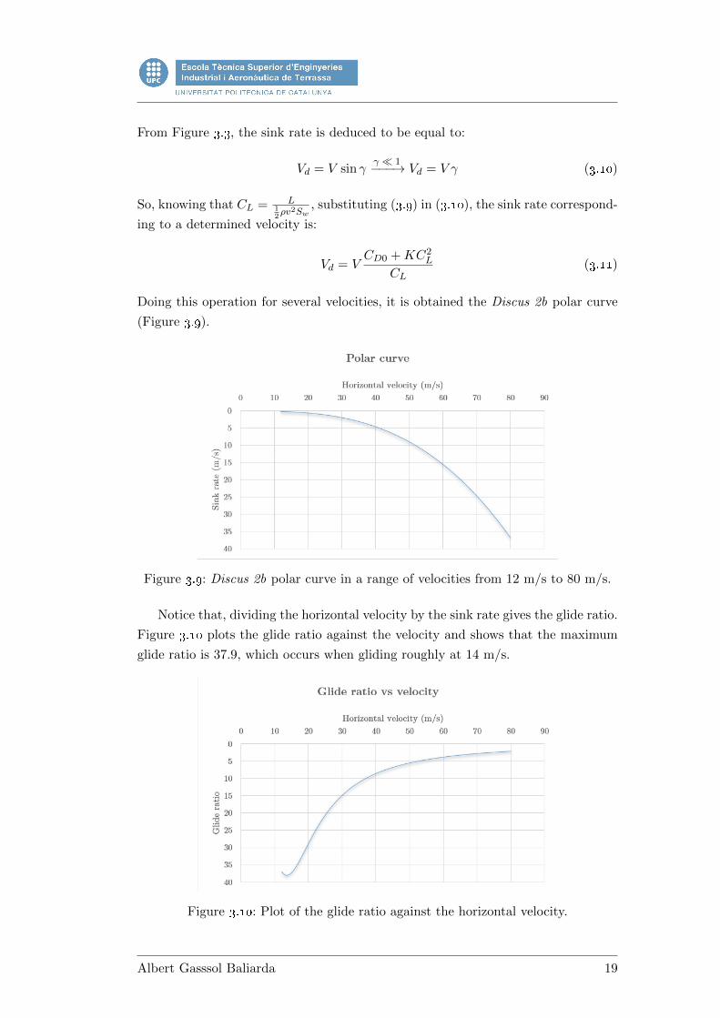
Doing this operation for several velocities, it is obtained the Discus 2b polar curve

(Figure 3.9).

Figure 3.9: Discus 2b polar curve in a range of velocities from 12 m/s to 80 m/s.

Notice that, dividing the horizontal velocity by the sink rate gives the glide ratio.

Figure 3.10 plots the glide ratio against the velocity and shows that the maximum

glide ratio is 37.9, which occurs when gliding roughly at 14 m/s.

Figure 3.10: Plot of the glide ratio against the horizontal velocity.


Chapter 4

Development

In the present chapter it is carried out all the aspects regarding to the drone flight,

since it is sent to high altitude by means of a weather balloon until it goes back

to land, according to what has been established in Chapter 3. This includes the

development of a physical model that describes the behaviour of the drone and a

control system that establishes the piloting rules at each moment and situation.

4.1 Weather balloon launching

A standard mission of the drone will always start with the launching of a weather

balloon where it will be attached to. There are lots of aspects to take into account

in this initial phase: the size of the balloon, the gas with which the balloon is filled

up, the ascent rate of the pack and so on. All these aspects about the launching of

the weather balloon will be dealt with in this section.

The physical principle that governs the ascent of a heavier-than-air object through

any fluid, such as the air, is the Archimedes’ principle, which establishes that “any

object, wholly or partially immersed in a fluid, is buoyed up by a force equal to the

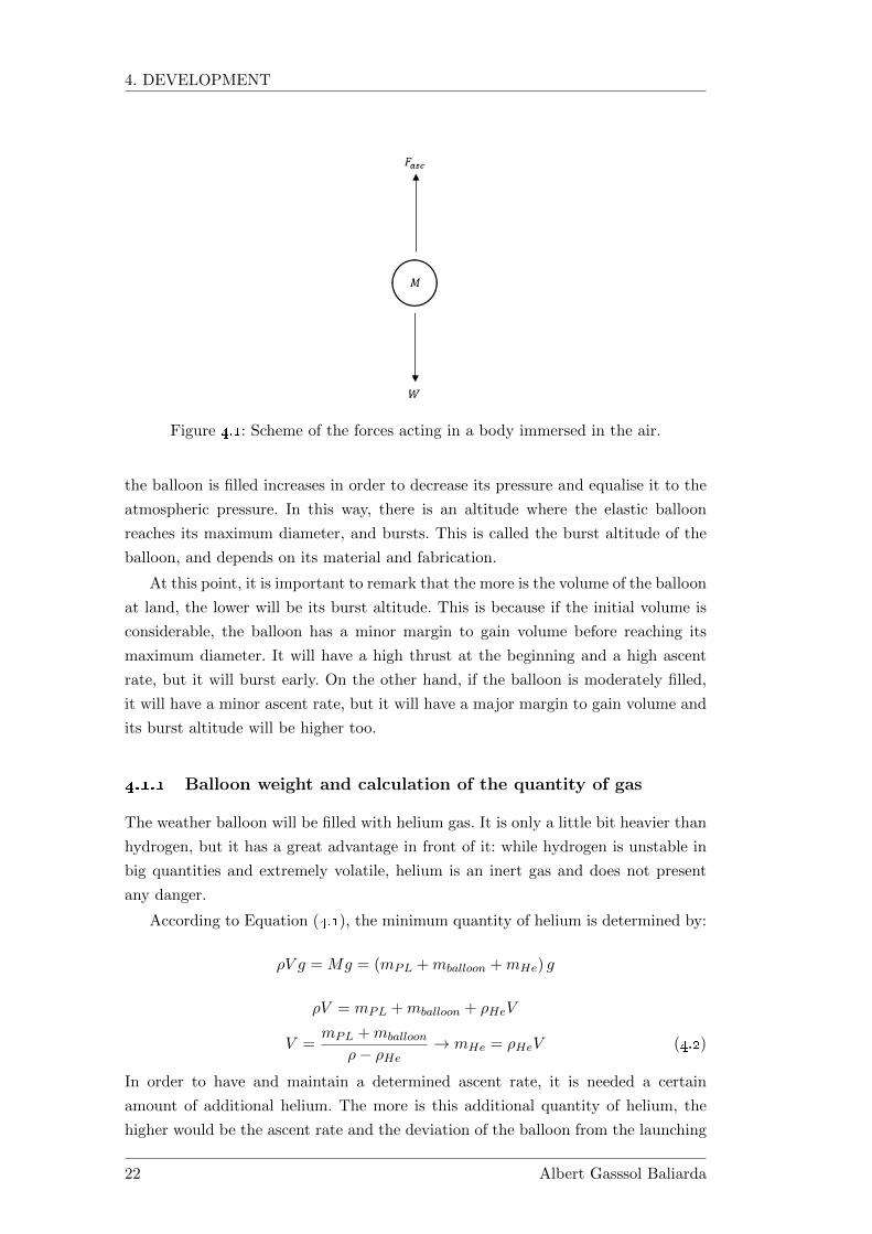
weight of the fluid displaced by the object”. In this way, setting out a scheme of

the forces acting on a body which is wholly immersed in the air (Figure 4.1) and

applying Newton’s second law, one obtains:

Fasc −W = Mdv

dt

ρV g −Mg = Mdv

dt(4.1)

However, the air density is not constant, and if the body immersed in the air

is an elastic balloon, its volume changes with altitude too [17]. This is because the

pressure inside the balloon must always be the same that the pressure outside. The

atmospheric pressure decreases with altitude, so the initial volume of gas with which


4. DEVELOPMENT

Figure 4.1: Scheme of the forces acting in a body immersed in the air.

the balloon is filled increases in order to decrease its pressure and equalise it to the

atmospheric pressure. In this way, there is an altitude where the elastic balloon

reaches its maximum diameter, and bursts. This is called the burst altitude of the

balloon, and depends on its material and fabrication.

At this point, it is important to remark that the more is the volume of the balloon

at land, the lower will be its burst altitude. This is because if the initial volume is

considerable, the balloon has a minor margin to gain volume before reaching its

maximum diameter. It will have a high thrust at the beginning and a high ascent

rate, but it will burst early. On the other hand, if the balloon is moderately filled,

it will have a minor ascent rate, but it will have a major margin to gain volume and

its burst altitude will be higher too.

4.1.1 Balloon weight and calculation of the quantity of gas

The weather balloon will be filled with helium gas. It is only a little bit heavier than

hydrogen, but it has a great advantage in front of it: while hydrogen is unstable in

big quantities and extremely volatile, helium is an inert gas and does not present

any danger.

According to Equation (4.1), the minimum quantity of helium is determined by:

ρV g = Mg = (mPL +mballoon +mHe) g

ρV = mPL +mballoon + ρHeV

V =mPL +mballoon

ρ− ρHe→ mHe = ρHeV (4.2)

In order to have and maintain a determined ascent rate, it is needed a certain

amount of additional helium. The more is this additional quantity of helium, the

higher would be the ascent rate and the deviation of the balloon from the launching


point will be minor, but the balloon needs to be larger too. If the balloon and its

payload have a determined ascent velocity, it appears an aerodynamic drag against

them, and Equation (4.1) in fact is:

ρV g −Mg − 1

2ρv2SCD = M

dv

dt(4.3)

To simplify calculations, it can be assumed the balloon to be a perfect sphere.

It can be considered too that the drag due to the payload is negligible compared to

that which affects the balloon. In this way, the drag coefficient of a smooth sphere

(weather balloons are mainly made of latex) depends on the Reynolds number Re

as shown in Figure 4.2.

Figure 4.2: Dependency of the drag coefficient of a sphere and the Reynolds num-ber [18].

In order to have a mean value of the drag coefficient for the current case, it has

been calculated an average Reynolds number, corresponding to which is obtained at

an altitude of 11000 m:

Re =ρ11vD11

µ11(4.4)

Re = 9.4× 105

where ρ11 = 0.364 kg/m3, v is taken as 8 m/s, D11 is the balloon diameter at

11000 m of altitude and µ11 = 1.42 × 10−5 Pa · s. For that Reynolds number, the

drag coefficient is determined then by [19]:

CD = 0.1 log10Re− 0.49 (4.5)

CD = 0.108

According to all of this, it has been developed a MATLAB script in order to see

the evolution of the balloon (this means, its altitude and ascent rate) as a function of

the quantity of helium which the balloon is filled with. The code is shown below, and


4. DEVELOPMENT

introducing a helium mass of 2.06 kg, the results are the ones shown in Figure 4.3.


1 clear

2 close a l l

3 clc

4

5 %% Data

6 P.M = 9 ; % Payload mass [ kg ]

7 P.Mb = 2 ; % Bal loon mass [ kg ]

8 P. g = 9 .80665 ; % Gravi t . a c c e l e r a t i o n [m/s ˆ2]

9 P. P0 = 101325; % Atmospheric pre s sure [Pa ]

10 P. rho0 = 1 . 2 2 5 ; % Air den s i t y [ kg/mˆ3]

11 P. rhoHe = 0 . 1 7 8 5 ; % Helium dens i t y [ kg/mˆ3]

12 P. VolMin = (P.M+P.Mb)/(P. rho0−P. rhoHe ) ; % Min . hel ium volume [mˆ3]

13 P. Vol0 = P. VolMin * 1 . 1 ; % Actual hel ium volume [mˆ3]

14 P. D0 = 2*(P. Vol0 /(4/3*pi ) ) ˆ ( 1 / 3 ) ; % I n i t i a l b a l l o on diameter [m]

15 P.mHe = P. Vol0*P. rhoHe ; % Helium mass [ kg ]

16 P.Mt = P.M+P.Mb+P.mHe; % Total mass to l i f t [ kg ]

17

18 % Ca l cu l a t i on o f the ba l l o on drag c o e f f i c i e n t ( assuming i t as a p e r f e c t

19 % sphere )

20

21 % Reynolds number at h = 11000 m

22 [ ˜ , ˜ , P11 , rho11 ] = ISA (11000 ) ; % [Pa ] , [ kg/mˆ3]

23 va = 8 ; % [m/s ]

24 Vol11 = P. P0*P. Vol0/P11 ; % Volume [mˆ3]

25 D11 = 2*( Vol11 /(4/3*pi ) ) ˆ ( 1 / 3 ) ; % Diameter [m]

26 mu11 = 1.42 e−5; % Dynamic v i s c o s i t y [Pa* s ]

27

28 Re11 = rho11*va*D11/mu11 ; % Mean Reynolds number

29

30 % Drag c o e f f i c i e n t

31 P.CD = 0.1* log10 ( Re11 )−0.49; % Bal loon drag c o e f f i c i e n t

32

33 %% So lu t i on

34 t i = 0 ; % [ s ]

35 t f = 2000 ; % [ s ]

36 tspan = [ t i , t f ] ;

37 x0 = [ 0 ; 0 ] ;

38 opt ions = odeset ( ) ;

39

40 [ tOut , xOut ] = ode45 ( @balloonPerformance , tspan , x0 , opt ions , P ) ;

41

42 f igure

43 subplot (2 , 1 , 1)

44 plot ( tOut , xOut ( : , 1 ) , ’ r ’ ) , grid on

45 xlabel ( ’Time ( s ) ’ ) , ylabel ( ’ A l t i tude (m) ’ )

46 subplot (2 , 1 , 2)


48 xlabel ( ’Time ( s ) ’ ) , ylabel ( ’ Ascent ra t e (m/ s ) ’ )

49

50 % At h = 20000 m


4. DEVELOPMENT

51 [ ˜ , ˜ , P20 , rho20 ] = ISA(20 e3 ) ;

52 Vol20 = P. P0*P. Vol0/P20 ;

53 D20 = 2*( Vol20 /(4/3*pi ) ) ˆ ( 1 / 3 ) ;

54

55 time = interp1 (xOut ( : , 1 ) , tOut , 20 e3 ) ;

56

57 % Average ascent ra t e

58 Va = 0 ;

59

60 for i =1: length (xOut ( : , 2 ) )

61 Va = Va+xOut ( i , 2 ) ;

62

63 end

64

65 avVa = Va/ length (xOut ( : , 2 ) ) ;

And the function balloonPerformance is:

1 function [ xdot ] = bal loonPerformance ( t , x , P)

2 % bal loonPerformance i s the d i f f e r e n t i a l equa t ion t ha t p r e d i c t s the

3 % evo l u t i on o f the a l t i t u d e and the ascent ra t e o f the weather ba l l o on .

4

5 [ ˜ , ˜ , Pa , rhoa ] = ISA ( x ( 1 ) ) ;

6 Vol = P. P0*P. Vol0/Pa ;

7 Rad = ( Vol /(4/3*pi ) ) ˆ ( 1 / 3 ) ;

8 S r e f = pi*Radˆ2 ;

9

10 L = Vol* rhoa*P. g ;

11 W = P. g*P.Mt ;

12 D = 0.5* rhoa*x (2)ˆ2* S r e f *P.CD;

13

14 xdot = [ x ( 2 ) ;

15 (L−W−D)/P.Mt ] ;

16

17 end

The mass of the balloon’s payload has been fixed in 9 kg. The drone model weighs

6.8 kg, but it have to be taken into account the systems, batteries and sensors and

the payload which the drone carries as well, so it has been fixed all this weight

in 9 kg, so far. The balloon mass is 2 kg, which actually is a heavy weight for a

latex balloon. Nevertheless, this is an appropriate balloon to lift a payload mass of

9 kg, because smaller balloons are not capable to lift such weight and reach its burst

diameter prematurely1.

So, to reach the 20000 m of altitude, the balloon takes almost 32 minutes (variable

time of the code above computes this magnitude), and at this altitude the balloon

diameter is 7.42 m (variable D20 ), which is smaller than the bursting diameter of

a standard 2000 g weather balloon [20]. Finally, the average ascent rate during the

whole ascent (variable avVa) is 11 m/s. Results are summarized in Table 4.1:

1See [20].


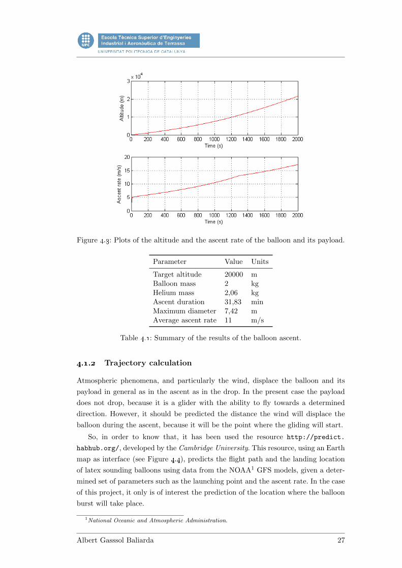
Figure 4.3: Plots of the altitude and the ascent rate of the balloon and its payload.


Target altitude 20000 mBalloon mass 2 kgHelium mass 2,06 kgAscent duration 31,83 minMaximum diameter 7,42 mAverage ascent rate 11 m/s

Table 4.1: Summary of the results of the balloon ascent.

4.1.2 Trajectory calculation

Atmospheric phenomena, and particularly the wind, displace the balloon and its

payload in general as in the ascent as in the drop. In the present case the payload

does not drop, because it is a glider with the ability to fly towards a determined

direction. However, it should be predicted the distance the wind will displace the

balloon during the ascent, because it will be the point where the gliding will start.

So, in order to know that, it has been used the resource http://predict.

habhub.org/, developed by the Cambridge University. This resource, using an Earth

map as interface (see Figure 4.4), predicts the flight path and the landing location

of latex sounding balloons using data from the NOAA1 GFS models, given a deter-

mined set of parameters such as the launching point and the ascent rate. In the case

of this project, it only is of interest the prediction of the location where the balloon

burst will take place.

1National Oceanic and Atmospheric Administration.


http://predict.habhub.org/

http://predict.habhub.org/

4. DEVELOPMENT

Figure 4.4: Interface of the habhub trajectory predictor.

In order to have an approximation of the order of magnitude of the distance at

which the balloon will be displaced by the wind, it has been ran the prediction fixing

the launching point at El Parc Natural de la Serra de Collserola, which coordinates

are 41.4388/2.1041. The rest of the parameters that have been set can be seen in

Table 4.2.


Launch site 41.4388/2.1041 CoordinatesLaunch altitude 0 mLaunch Time 12:00 UTC TimeLaunch Date 2015-05-20 DateAscent rate 11 m/sBurst altitude 20000 mDescent rate 15 m/s

Table 4.2: Configuration of the parameters with which has been ran the trajectorysimulation.

Simulation

Figure 4.5 shows the results of the trajectory simulation of the balloon. The burst

point is at a distance of 20.5 km from the launching point, concretely at coordinates

41.4623/2.3607. The balloon is displaced eastward and just a little northward. This

is obviously just one simulation and the results may be quite different depending on

the season and the meteorology of each day, but it can be used as an approximation

to know the order of magnitude of how much this distance can be.


Figure 4.5: Simulation of the trajectory of the balloon (from the origin to the burstpoint).

4.2 Creation of a model

In this section it is explained in detail the model that is used to simulate the be-

haviour of the drone since the moment when the weather balloon where it is attached

bursts (or when the drone is set free if the balloon does not burst when it is desired).

The creation of this model includes, on the one hand, a mathematical way to rep-

resent the environment in which the drone operates. This environment is basically

the atmosphere, with its variations of temperature, pressure and density with the

altitude and the strong winds that take place at determined altitudes, as it has been

seen in Chapter 3. On the other hand, the creation of the model means to set out

all the equations that rule a glider’s flight and all the characteristics that affect the

performances of the actual glider, the Discus 2b model.

So, in the present section first it is explained how it has been modelled the

environment, and afterwards it is developed the glider dynamics model which is

used. Finally, it is explained how it has been done the integration of both parts and

how does it work all together. The computational implementation of these models

has been done with the MATLAB software, under an educational license provided

by the Polytechnic University of Catalonia.

4.2.1 Environment modelling

The modelling of the environment has basically to take into account the physical

properties of the air and the wind that it may exist, as well as its variations. For

the physical properties of the air it is used the already mentioned International

Standard Atmosphere (ISA) model. It considers the air to be at rest with respect

to the Earth, and variations of its properties only take place in the vertical plane.

The detailed information of the ISA model can be seen in Appendix A, as well as

its computational implementation.


4. DEVELOPMENT

Regarding the atmospheric winds, with no loss of generality, it is considered a

wind profile which is a function of the altitude and blows from West to East. As

it has been seen in Chapter 3, the strongest winds usually are, in the local zone,

at altitudes between 7 km and 12 km, with an average maximum speed of 70 kt

(see Appendix B). In this way, it is assumed a model which establishes a wind with

a stationary velocity of 70 kt (36 m/s) in the interval of altitudes of 7 − 12 km.

The wind gradient from zero velocity to its maximum can be defined as a quadratic

variation with a determined average wind gradient slope [21], so that this average

gradient slope is:

β =Vw,maxhtr

(4.6)

where Vw,max = 36 m/s and htr is the transition vertical distance in which the wind

passes from 0 to be constant, which is established in 1 km. Then, the following

dimensionless variables are defined:

Vw =Vw

Vw,max, h =

h− 6× 103

htr(4.7)

And a linear wind gradient profile can be expressed as:

Vw = h→ Vw = β(h− 6× 103

)(4.8)

A quadratic expression of the wind gradient profile with the average gradient

slope of (4.8) is given by:

Vw = Ah+ (1−A) h2 (4.9)

Notice that Vw = 0 at h = 0 and Vw = 1 at h = 1. Substituting (4.7) in (4.9), the

final expression of the quadratic wind gradient profile is obtained:

Vw = β

[A(h− 6× 103

)+

1−Ahtr

(h− 6× 103

)2](4.10)

In order to ensure that Vw ∈ [0, Vw,max], it is requested that 0 < A < 2. If 0 < A < 1,

the quadratic profile has a concave shape, while if 1 < A < 2 the gradient profile is

convex. For A = 1 the profile is a straight line. It has been taken A = 0 in order to

make more progressively the adaptation of the wind profile where Vw = 0.

For the second wind gradient, which passes from the maximum velocity to zero

in a transition height of 1 km, the expression is quite similar to (4.10), with some

differences:

Vw = Vw,max − β[A(h− 12× 103

)+

1−Ahtr

(h− 12× 103

)2](4.11)

being in this case A = 2. Then, the wind profile can be seen in Figure 4.6.

The computational implementation of this wind profile is shown below. It consists


Figure 4.6: Wind profile with its quadratic wind gradient, blowing easterwards.

on a MATLAB function called windField, which from the altitude h as the only input

returns a first array with the components of the wind in Earth-axes (actually only

the y component is different from zero) and another one with the derivative of wind

with respect to height, which is needed for the glider equations of motion that are

developed later on. This derivative is approximated by:

dVw(h)

dh=Vw(h+ δ)− Vw(h)

δ(4.12)

where δ = 10−2.

1 function [ windEA , dwindEAdh ] = windFie ld (h)

2 % windFie ld e s t a b l i s h e s the e x i s t i n g atmospheric wind f i e l d as a func t i on

3 % of the h e i g h t . The wind f i e l d i s g i ven in Earth a x i s . This f unc t i on

4 % a l s o re turns the d e r i v a t i v e e o f the wind speed wi th r e s p e c t the

5 % he i g h t .

6 % The wind model c o n s i s t s on a West to East wind p r o f i l e which changes

7 % with a l t i t u d e accord ing to :

8 % 0−7 km: Wind = 0

9 % 7−8 km: Quadratic v a r i a t i on from 0 to 70 k t s

10 % 8−12 km: Wind = 70 k t s

11 % 12−13 km: Quadratic v a r i a t i on from 70 k t s to 0

12 % 13− i n f km: Wind = 0

13

14 wPeak kts = 70 ; % [ k t s ]

15 wPeak = 0.51444* wPeak kts ; % [m/s ]

16 hIn i1 = 6e3 ; % [m]

17 hFin1 = 7e3 ; % [m]

18 htr1 = hFin1−hIn i1 ; % [m]

19 hIn i2 = 12 e3 ; % [m]


4. DEVELOPMENT

20 hFin2 = 13 e3 ; % [m]

21 htr2 = hFin2−hIn i2 ; % [m]

22

23 beta1 = wPeak/ htr1 ; % [ sˆ−1]24 beta2 = wPeak/ htr2 ; % [ sˆ−1]25 A1 = 0 ;

26 A2 = 2 ;

27

28 % windEA

29 switch l o g i c a l ( t rue )

30 case h >= hIn i1 && h <= hFin1

31 Wy = beta1 *(A1*(h−hIn i1 )+(1−A1)/ htr1 *(h−hIn i1 ) ˆ 2 ) ;

32

33 case h > hFin1 && h < hIn i2

34 Wy = wPeak ;

35

36 case h >= hIn i2 && h <= hFin2

37 Wy = wPeak−beta2 *(A2*(h−hIn i2 )+(1−A2)/ htr2 *(h−hIn i2 ) ˆ 2 ) ;

38

39 otherwi s e

40 Wy = 0 ;

41

42 end

43

44 Wx = 0 ;

45 Wz = 0 ;

46

47 windEA = [Wx, Wy, Wz] ; % [m/s ]

48

49 % dwindEAdh

50 deltaH =0.01; % [m]

51 hPrima = h+deltaH ; % [m]

52


54 case hPrima >= hIn i1 && hPrima <= hFin1

55 Wy2 = beta1 *(A1*( hPrima−hIn i1 )+(1−A1)/ htr1 *( hPrima−hIn i1 ) ˆ 2 ) ;

56

57 case hPrima > hFin1 && hPrima < hIn i2

58 Wy2 = wPeak ;

59

60 case hPrima >= hIn i2 && hPrima <= hFin2

61 Wy2 = wPeak−beta2 *(A2*( hPrima−hIn i2 )+(1−A2)/ htr2 *( hPrima−hIn i2 ) ˆ 2 ) ;

62

63 otherwi s e

64 Wy2 = 0 ;

65

66 end

67

68 dWydh = (Wy2−Wy)/ deltaH ;

69


70 dWxdh = 0 ;

71 dWzdh = 0 ;

72

73 dwindEAdh = [dWxdh, dWydh, dWzdh ] ; % [ sˆ−1]74

75 end

4.2.2 Glider dynamics modelling

In order to study the drone dynamics, it has been developed a point-mass model

which simulates the motion of the drone’s centre of gravity throughout its trajectory.

So, in this project it is just studied the glider’s performances considering it as a point-

mass, leaving the stability issues for another phase of the design. In this way, the

following hypotheses have been done:

� The Earth is considered as a flat surface and taken as an inertial reference

system, so the centrifugal and Coriolis accelerations due to its rotation are not

taken into account.

� The winds that take place during the flight are stationary and only depend on

the altitude.

� It is assumed symmetric flight in the whole gliding, which means that the

sideslip angle always equals zero:

β = 0 ∀t

The set of equations that describes the glider motion is composed by three kine-

matic relations and three dynamic ones. The three kinematic relations are expressed

in the Earth-axes reference system. The origin point of this reference system is an

arbitrary point placed on the Earth’s surface. The xe-axis points to an arbitrary

and fixed direction (e.g., the North), the ze-axis points to the centre of the Earth

and the ye-axis completes a Cartesian right-handed reference system (in this case it

points to the East) [22]. So, the three kinematic relations are:

xe = v cos γ cosχ

ye = v cos γ sinχ+ Vw

ze = −v sin γ

(4.13)

(4.14)

(4.15)

where v is the norm of the aerodynamic velocity, χ is the yaw angle measured

clockwise from the North in wind axes and γ is the air-relative flight path angle.

The dynamic relations are obtained by applying the Newton’s second law to the

forces acting on the glider in the wind-axes reference system. In the wind-axes refer-

ence system, the xw-axis points according to the instantaneous aerodynamic velocity


4. DEVELOPMENT

vector, the zw-axis is contained in the aircraft symmetry plane and is perpendicular

to the xw-axis pointing down and the yw-axis completes the Cartesian right-handed

reference system. In this way, it results:

∑ −→F∣∣∣w

= md−→V

dt

∣∣∣∣∣w

= md−→vdt

∣∣∣∣w

+ md−→Vwdt

∣∣∣∣∣w

(4.16)

where−→V is the glider velocity with respect the ground,−→v is the aerodynamic velocity

and−→Vw is the wind velocity. The forces acting on a non-propelled glider are the lift

L, the aerodynamic drag D and the weight W . The first ones are expressed in

wind-axes, while the weight is known in Earth-axes:

∑ −→F∣∣∣w

=(−D 0 −L

)iw

jw

kw

+(

0 0 W)

ie

je

ke

(4.17)

Using the Euler’s angles [23], it is possible to pass from the Earth-axes reference

system to the wind-axes reference system by means of a rotation matrix:iejeke

= Lew

iwjwkw

(4.18)

being Lew:

Lew =

cos γ cosχ sinµ sin γ cosχ− cosµ sinχ cosµ sin γ cosχ+ sinχ sinµ

cos γ sinχ sinµ sin γ sinχ+ cosχ cosµ cosµ sin γ sinχ− sinµ cosχ

− sin γ sinµ cos γ cosµ cos γ

where µ is the glider’s roll angle. So, applying (4.18) on (4.17), it yields:

∑ −→F∣∣∣w

=(−D 0 −L

)iw

jw

kw

+(

0 0 W)Lew

iw

jw

kw

∑ −→

F∣∣∣w

=(−D −W sin γ W sinµ cos γ −L+W cosµ cos γ

)iw

jw

kw

(4.19)

The first term of the right side of Equation (4.16) is calculated as follows:

md−→vdt

∣∣∣∣w

= m

v00

+m

pwqwrw

∧v0

0

=

mv

mrwv

−mqwv

(4.20)


where pw, qw and rw are the rotation velocities of the wind-axes reference system.

The last term of Equation (4.16) is calculated by:

d−→Vwdt

∣∣∣∣∣e

=(

0 Vw 0)

ie

je

ke

→ d−→Vwdt

∣∣∣∣∣w

=(

0 Vw 0)Lew

iw

jw

kw

md−→Vwdt

∣∣∣∣∣w

=

mVw

(cos γ sinχ sinµ sin γ sinχ+ cosχ cosµ cosµ sin γ sinχ− sinµ cosχ

)iw

jw

kw

(4.21)

Notice that Vw only depends on the altitude, so the term Vw is calculated doing:

Vw =dVwdh

dh

dt=

dVwdh

v sin γ

With all of this, the three dynamic relations are:−D −mg sin γ = m

(v + Vw cos γ sinχ

)mg cos γ sinµ = m

(rwv + Vw sinµ sin γ sinχ+ Vw cosχ cosµ

)− L+mg cos γ cosµ = m

(−qwv + Vw cosµ sin γ sinχ− Vw sinµ cosχ

)(4.22)

(4.23)

(4.24)

In a similar way of what has already been done, by means of the Euler angles it is

possible to convert pw, qw and rw to χ, γ and µ1, and the following is obtained:χ =

1

cos γ(qw sinµ+ rw cosµ)

γ = qw cosµ− rw sinµ

µ = pw + (qw sinµ+ rw cosµ) tan γ

(4.25)

(4.26)

(4.27)

Replacing rw from (4.23) and qw from (4.24) to (4.25) and (4.26), together with

Equation (4.22) and the three kinematic relations, it is obtained the 6 differential

1See [23].


4. DEVELOPMENT

equations of motion:

xe = v cos γ cosχ

ye = v cos γ sinχ+ Vw

ze = −v sin γ

γ = qw cosµ− rw sinµ

χ = 1cos γ (qw sinµ+ rw cosµ)

v = 1m

(−D −mg sin γ −mVw cos γ sinχ

)(4.28)

These equations can be expressed as:

−→x = f

(−→x ,−→u ) (4.29)

where −→x is the state vector and −→u is the control vector, which includes the variables

that control the rest of the variables that are defined in the state vector and that

define the motion of the drone.

−→x =

xe

ye

ze

γ

χ

v

, −→u =

[α

µ

](4.30)

Particularization of the case

The previous model predicts the motion of the glider in a continuous flight, whatever

is the value of the motion variables and its derivatives. However, this model needs to

be particularized, because the actual flight starts with the drone ascending attached

to a weather balloon and then initiating a descent without any velocity when it is

reached the desired altitude.

So, it would be a good option to attach the drone to the weather balloon by its

tail in such a way that, when the balloon bursts, the glider starts a vertical nose

diving. Then, when it reaches a proper velocity to start the gliding, it should increase

its flight path angle –which until this moment equals γ = –π/2 –by means of the

control system in order to get a normal flight attitude and start the actual gliding.

This is done by increasing progressively the angle of attack, as it is described in

Section 4.3.

The velocity at which the control system begins to control the drone will be

fixed in 100 kt, which is a velocity quite major than the maximum wind velocity

that has been established in the environment modelling. This is because this one is

a theoretical model, but actually wind speeds could be greater than the fixed 70 kt


in determined occasions, or even they can occur at higher and lower altitudes that

what the model establishes. So if it is possible, it is of great importance to ensure the

drone has the capability to fly at high speeds as soon as possible. According to this,

this vertical nose diving is mathematically governed by the following expression:

mg −D = mdv

dt(4.31)

where D = 12ρv

2SwCD0 because in this situation CL = 0, and the induced drag

equals zero as well. In order to know the time that the drone takes to reach a speed

of 100 kt and the vertical distance that it drops in this time, the following MATLAB

script has been developed:

1 clear a l l

2 close a l l

3 clc

4

5 P.Sw = 0 . 6 5 3 ; % [mˆ2]

6 P.M = 9 ; % [ kg ]

7 P.CD0 = 0 . 0 1 2 ;

8 P. g = 9 .8066 5 ; % [m/s ˆ2]

9

10

11 tspan = [ 0 , 3 0 ] ;

12 noseDive0 = [20 e3 ; 0 ] ;

13 opt ions = odeset ( ) ;

14

15 [ ta , xa ] = ode45 ( @noseDiveFcn , tspan , noseDive0 , opt ions , P ) ;

16

17 f igure

18 subplot ( 2 , 1 , 1 )

19 plot ( ta , xa ( : , 1 ) , ’ r ’ )


21 grid on

22 subplot ( 2 , 1 , 2 )

23 plot ( ta , xa ( : , 2 ) , ’ r ’ )

24 xlabel ( ’Time ( s ) ’ ) , ylabel ( ’ Ve loc i ty (m/ s ) ’ )

25 grid on

26

27 % Compute the time and a l t i t u d e at which i t i s reached a v e l o c i t y o f 100 k t s

28 v = 100*0 .51444 ; % [m/s ]

29 time = interp1 ( xa ( : , 2 ) , ta , v ) ;

30 h = interp1 ( xa ( : , 2 ) , xa ( : , 1 ) , v ) ;

And the noseDiveFcn function is:

1 function xdot = noseDiveFcn ( t , x , s t r u c t )

2

3 Sw = s t r u c t .Sw ;

4 M = s t r u c t .M;

5 CD0 = s t r u c t .CD0;


4. DEVELOPMENT

6 g = s t r u c t . g ;

7

8 [ ˜ , ˜ , ˜ , rho ] = ISA ( x ( 1 ) ) ;

9

10 xdot = [−x ( 2 ) ;

11 (M*g−0.5* rho*x (2)ˆ2*Sw*CD0)/M] ;

12

13 end

This gives the following results (see Figure 4.7):

t = 5.26 s, h = 19864 m

As it can be seen, the drone spends very little time to reach 100 kt, and it drops

very little height too.

Figure 4.7: Evolution of the altitude and the dive velocity starting at h = 20000 mwith v = 0.

Computational implementation

The computational implementation of the glider dynamics model particularized for

the current case is based on a main MATLAB script which initializes all the data

and variables that are needed to simulate and control the model. Then, it calls a

solver for ordinary differential equations (in this case it is used the ode23 solver) that

integrates the equations of motion previously established. Finally, it plots the results,

displaying in one first plot, the trajectory that follows the drone in a 3D-view, and

in a second plot, the temporal evolution of the flight altitude, the air-relative flight

path angle, the distance from the launching location (which is the landing location

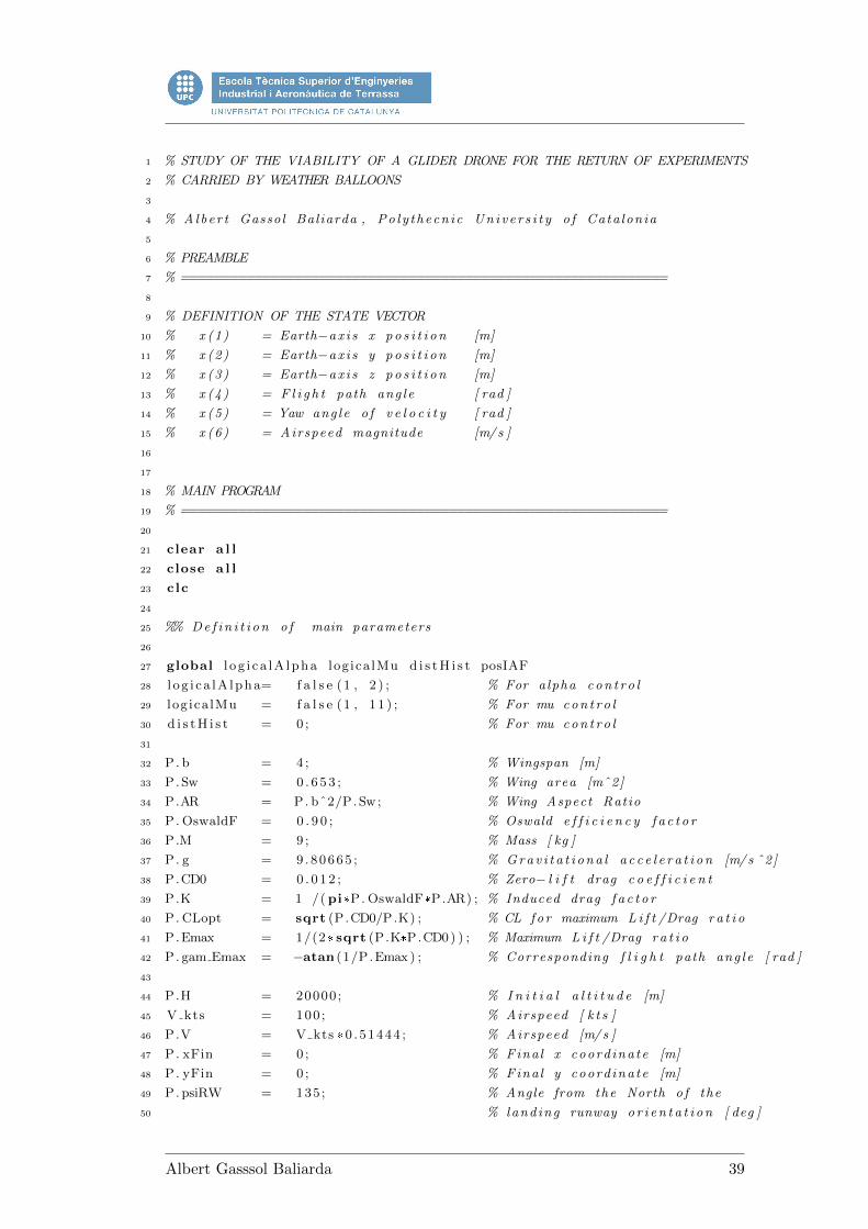
as well) and the aerodynamic velocity. This main script is shown below.


1 % STUDY OF THE VIABILITY OF A GLIDER DRONE FOR THE RETURN OF EXPERIMENTS

2 % CARRIED BY WEATHER BALLOONS

3

4 % Alber t Gassol Bal iarda , Po l y thecn i c Un i v e r s i t y o f Cata lonia

5

6 % PREAMBLE

7 % ============================================================

8

9 % DEFINITION OF THE STATE VECTOR

10 % x (1) = Earth−ax i s x p o s i t i o n [m]

11 % x (2) = Earth−ax i s y p o s i t i o n [m]

12 % x (3) = Earth−ax i s z p o s i t i o n [m]

13 % x (4) = F l i g h t path ang l e [ rad ]

14 % x (5) = Yaw ang le o f v e l o c i t y [ rad ]

15 % x (6) = Airspeed magnitude [m/s ]

16

17

18 % MAIN PROGRAM

19 % ============================================================

20

21 clear a l l

22 close a l l

23 clc

24

25 %% De f i n i t i on o f main parameters

26

27 global l o g i c a lA lpha log ica lMu d i s t H i s t posIAF

28 l o g i c a lA lpha= f a l s e (1 , 2 ) ; % For a lpha con t r o l

29 log ica lMu = f a l s e (1 , 1 1 ) ; % For mu con t r o l

30 d i s t H i s t = 0 ; % For mu con t r o l

31

32 P. b = 4 ; % Wingspan [m]

33 P.Sw = 0 . 6 5 3 ; % Wing area [mˆ2]

34 P.AR = P. bˆ2/P.Sw ; % Wing Aspect Ratio

35 P. OswaldF = 0 . 9 0 ; % Oswald e f f i c i e n c y f a c t o r

36 P.M = 9 ; % Mass [ kg ]

37 P. g = 9 .8066 5 ; % Grav i t a t i ona l a c c e l e r a t i o n [m/s ˆ2]

38 P.CD0 = 0 . 0 1 2 ; % Zero− l i f t drag c o e f f i c i e n t

39 P.K = 1 /(pi*P. OswaldF*P.AR) ; % Induced drag f a c t o r

40 P. CLopt = sqrt (P.CD0/P.K) ; % CL fo r maximum L i f t /Drag r a t i o

41 P.Emax = 1/(2* sqrt (P.K*P.CD0 ) ) ; % Maximum L i f t /Drag r a t i o

42 P. gam Emax = −atan (1/P.Emax ) ; % Corresponding f l i g h t path ang l e [ rad ]

43

44 P.H = 20000; % I n i t i a l a l t i t u d e [m]

45 V kts = 100 ; % Airspeed [ k t s ]

46 P.V = V kts *0 . 51444 ; % Airspeed [m/s ]

47 P. xFin = 0 ; % Fina l x coord ina te [m]

48 P. yFin = 0 ; % Fina l y coord ina te [m]

49 P. psiRW = 135 ; % Angle from the North o f the

50 % land ing runway o r i e n t a t i on [ deg ]


4. DEVELOPMENT

51

52 P. alpha0 = −0.060666; % AoA corresponding to CL = 0 [ rad ]

53 P.CLmax = 1 . 3 3 3 1 ; % CLmax

54 P. CLmin = −0.6799; % CLmin

55

56 P. c o n t r o l = @controlFcn ; % Contro l System

57

58 %% I n i t i a l i z a t i o n o f the S ta t e v e c t o r

59

60 xe = 25 e3 ; % [m]

61 ye = 25 e3 ; % [m]

62 ze = −P.H; % [m]

63 gamRad = −pi /2 ; % [ rad ]

64 chiRad = pi ; % [ rad ]

65 v = 0 ; % [m/s ]

66

67 x0 = [ xe ;

68 ye ;

69 ze ;

70 gamRad ;

71 chiRad ;

72 v ] ;

73

74 %% Simulat ion

75

76 t i = 0 ; % [ s ]

77 t f = 5 .50*3600 ; % [ s ]

78 tspan = [ t i , t f ] ;

79 opt ions = odeset ( . . .

80 ’ Re f ine ’ , 2 , . . .

81 ’ Events ’ , @eventFcn ) ;

82

83 [ tOut , xOut ] = ode23 ( @flightMechEqs , tspan , x0 , opt ions , P ) ;

84

85 %% Plo t s

86

87 Distance = zeros ( length (xOut ) , 1 ) ;

88

89 for i =1: length (xOut )

90 xx = xOut ( i , 1 ) ;

91 yy = xOut ( i , 2 ) ;

92 posVec = [P. xFin−xx , P. yFin−yy ] ;

93 Distance ( i ) = norm( posVec ) ;

94

95 end

96

97 f igure

98 plot3 (xOut ( : , 1 ) , xOut ( : , 2 ) , −xOut ( : , 3 ) , ’ r ’ )

99 xlabel ( ’ North ’ ) , ylabel ( ’ East ’ ) , zlabel ( ’ A l t i tude ’ )

100 grid on


101

102 f igure

103 subplot ( 2 , 2 , 1 )

104 plot ( tOut ,−xOut ( : , 3 ) , ’ r ’ ) , grid on


106 subplot ( 2 , 2 , 2 )


108 xlabel ( ’Time ( s ) ’ ) , ylabel ( ’ F l i gh t Path Angle ( rad ) ’ )

109 subplot ( 2 , 2 , 3 )

110 plot ( tOut , Distance , ’ r ’ ) , grid on

111 xlabel ( ’Time ( s ) ’ ) , ylabel ( ’ Hor i zonta l d i s t ance from the land ing po int (m) ’ )

112 subplot ( 2 , 2 , 4 )


114 xlabel ( ’Time ( s ) ’ ) , ylabel ( ’ Ve loc i ty (m/ s ) ’ )

As it can be seen, the main parameters (e.g. mass, aspect ratio, etc.) are stored

in a structure called P. The declared global variables are just needed for control

purposes, and their function are explained later on. Following, it is initialized the

state vector, which afterwards is used as the vector of initial conditions for the ode23

solver:

−→x =

25× 103

25× 103

−20× 103

−π/2π

0

The initials xe and ye are the deviation from the launching point that the drone

and the weather balloon experience until they reach the desired altitude. The value

of ze is negative because the ze-axis points down, and γ and v are consequence of

the initial nose diving with zero initial velocity. The value of χ is arbitrary, but in

this case the glider would point to the South. Finally, the ode23 solver calls the

equations of motion –which are defined in the MATLAB function flightMechEqs –

and integrates them, simulating the entire flight until ze = 0, and the results are

plotted.

The equations of motion are implemented in the flightMechEqs function:

1 function [ xdot ] = f l ightMechEqs ( t , x , s t r u c t )

2 % f l i gh tMechEqs i s the system of d i f f e r e n t i a l e qua t i ons t ha t d e s c r i b e s

3 % the motion o f a point−mass g l i d i n g , assuming f l a t Earth ,

4 % s t a t i ona r y winds ( on ly in the ye d i r e c t i o n ) and symmetric f l i g h t .

5 % Equations :

6 % (1) dx/ dt = v* cos (gamma)* cos ( ch i )

7 % (2) dy/ dt = v* cos (gamma)* s in ( ch i )+Wy

8 % (3) dz/ dt = −v* s in (gamma)

9 % (4) d (gamma)/ dt = q* cos (mu)−r* s in (mu)

10 % (5) d ( ch i )/ dt = 1/ cos (gamma)*( q* s in (mu)+r* cos (mu))

11 % (6) du/ dt = 1/M*(−D−M*g* s in (gamma)−M*Wydot* cos (gamma)* cos (mu))


4. DEVELOPMENT

12 %

13 % L = 0.5* rho*uˆ2*Sw*CL

14 % D = 0.5* rho*uˆ2*Sw*CD

15

16 global l o g i c a lA lpha

17

18 M = s t r u c t .M;

19 g = s t r u c t . g ;


21 V = s t r u c t .V;

22

23 [ alphaRad , muRad ] = contro lFcn ( t , x , s t r u c t ) ;

24 [CL, CD] = ae roCoe f f s ( alphaRad , s t r u c t ) ;

25 [ windEA , dWdh] = windFie ld(−x ( 3 ) ) ;

26 [ ˜ , ˜ , ˜ , rho ] = ISA(−x ( 3 ) ) ;

27 L = 0.5* rho*x (6)ˆ2*Sw*CL;

28 D = 0.5* rho*x (6)ˆ2*Sw*CD;

29

30 % dW/dt = (dW/dh )*( dh/ dt )

31 % Wxdot = 0 , Wzdot = 0

32 Wydot = dWdh(2)* x (6)* sin ( x ( 4 ) ) ;

33

34 % p & q

35 q = 1/(M*x ( 6 ) )* ( L−M*g*cos ( x (4 ) )* cos (muRad)+M*Wydot*( cos (muRad)* sin ( x ( 4 ) ) . . .

36 * sin ( x(5))− sin (muRad)* cos ( x ( 5 ) ) ) ) ;

37 r = 1/(M*x ( 6 ) )* (M*g*cos ( x ( 4 ) )* sin (muRad)−M*Wydot*( sin (muRad)* sin ( x ( 4 ) ) * . . .

38 sin ( x (5))+ cos ( x (5 ) )* cos (muRad ) ) ) ;

39

40

41 i f l o g i c a lA lpha (1 ) == f a l s e % v never has been major than V

42 i f x (6 ) < V

43 xdot = [ x (6)* cos ( x (4 ) )* cos ( x ( 5 ) ) ;

44 x (6)* cos ( x (4 ) )* sin ( x (5))+windEA ( 2 ) ;

45 −x (6)* sin ( x ( 4 ) ) ;

46 0 ;

47 0 ;

48 1/M*(−D−M*g* sin ( x(4))−M*Wydot*cos ( x (4 ) )* cos (muRad ) ) ] ;

49

50 else

51 xdot = [ x (6)* cos ( x (4 ) )* cos ( x ( 5 ) ) ;


53 −x (6)* sin ( x ( 4 ) ) ;

54 q*cos (muRad)−r * sin (muRad ) ;

55 0 ;


57

58 l o g i c a lA lpha (1 ) = true ;

59

60 end

61


62 else

63 i f l o g i c a lA lpha (2 ) == f a l s e % gamma never has been major than −p i /464 i f x (4 ) < −pi/4

65 xdot = [ x (6)* cos ( x (4 ) )* cos ( x ( 5 ) ) ;


67 −x (6)* sin ( x ( 4 ) ) ;


69 0 ;


71

72 else

73 xdot = [ x (6)* cos ( x (4 ) )* cos ( x ( 5 ) ) ;


75 −x (6)* sin ( x ( 4 ) ) ;


77 1/cos ( x ( 4 ) )* ( q* sin (muRad)+r *cos (muRad ) ) ;


79

80 l o g i c a lA lpha (2 ) = true ;

81

82 end

83

84 else

85 xdot = [ x (6)* cos ( x (4 ) )* cos ( x ( 5 ) ) ;


87 −x (6)* sin ( x ( 4 ) ) ;


89 1/cos ( x ( 4 ) )* ( q* sin (muRad)+r *cos (muRad ) ) ;


91

92 end

93

94 end

95

96 end

In this function it appears two other new functions: the controlFcn and aeroCoeffs

functions. The first one is included in the P structure and represents the drone’s

control system, so it is the function in charge of giving a value to the control variables

–µ and α –and it is explained in detail in Section 4.3. The other one returns the

value of the lift and drag coefficients of the drone corresponding to a given angle of

attack, according to the aerodynamic characteristics of the Discuss 2b wing airfoil

that have been established in Chapter 3. This function is the following:

1 function [CL, CD] = ae roCoe f f s ( alphaRad , s t r u c t )

2 % aeroCoe f f s r e tu rns the aerodynamic c o e f f i c i e n t s CL and CD corresponding

3 % to a wing wi th a determined Aspect Ratio (AR) based on the

4 % aerodynamic a i r f o i l HQ 2.5/12 at Re = 5e5 . Appl ied data corresponds

5 % to the in format ion a v a i l a b l e a t wwww. a i r f o i l t o o l s . com .

6


4. DEVELOPMENT

7 AR = s t r u c t .AR;

8 alpha0 = s t r u c t . alpha0 ;


10 K = s t r u c t .K;

11

12 CLmax = 1 . 3 3 3 1 ;

13 CLmin = −0.6799;

14 CL0 = 0 . 3 2 8 9 ;

15 Clalpha = 5 . 8 9 5 7 ;

16 CLalpha = Clalpha /(1+ Clalpha /(pi*AR))*(1−1e−2);

17 CLPrima = CL0+CLalpha*alphaRad ;

18

19 i f alphaRad == alpha0

20 CL = 0 ;

21

22 else

23 i f CLPrima >= CLmin && CLPrima <= CLmax

24 CL = CLPrima ;

25

26 else

27 fpr intf ( ’ Error : CL not p o s s i b l e . ’ ) ;

28

29 end

30

31 end

32

33 CD = CD0+K*CLˆ2 ;

34

35 end

The general equations of motion are the set of equations (4.28), but when working

with numerical methods it is needed to do something in order to avoid the singularity

that appears in the χ expression when γ = ±π/2. With this purpose, it has been

defined the global variable logicalAlpha, which is a Boolean array of dimension 2

that initially is set to false. So, when the drone is executing the nose diving, the

equations of χ and γ have been omitted, because both variables do not change in

this first phase (the control system does not provide neither roll angle nor angle

of attack), and the first one produces a singularity in the system of equations that

must be avoided.

When the drone reaches for first time a velocity equal or greater than 100 kt, the

first component of the Boolean array logicalAlpha becomes true. At this moment,

the control system progressively increases the angle of attack (see Section 4.3), and

the equations of motion are modified in such a way that now they allow changes in

the flight path angle. In this way, the flight path angle starts to rise, and when it is

equal or major than –π/4, the last component of the logicalAlpha array becomes true

too and the equations change again, adding the expression of χ, so it finally yields

the complete system of equations of motion. At this moment, the control system


can provide roll angle too, and the drone can change of direction according to the

piloting rules.

Figure 4.8 attempts to explain this sequence, and Figure 4.9 shows the results

of the simulation of this initial stage, fixing the roll angle to µ = 0.

Figure 4.8: Sequence of the drone’s gliding start.

Figure 4.9: Trajectory of the drone in the firsts 10 minutes, flying without rolling.

4.3 The control system

The control system is the function in charge of piloting the drone so that its response

is as expected at any situation. So, as a function of the state vector, the time and the

own parameters of the drone, the control system establishes the control parameters

that will define the drone response. In this case, the control parameters are the

angle of attack and the roll angle. The first one controls the longitudinal attitude of

the drone, which in the current point-mass model is actually the flight path angle,

i.e. the sink rate. With the roll angle it is controlled the directional attitude, so

it has a direct effect on the drone’s yaw angle. In more advanced dynamic models

based on rigid body dynamics, the control system runs orders to the electronic


4. DEVELOPMENT

and hydraulic devices that drive the drone’s control surfaces, and are the moments

generated by these control surfaces which actually produce a drone response (that

can be an angular acceleration, a pitch movement that stabilizes the drone, etc.). A

rigid body-like control system requires a more detailed knowledge about the drone

characteristics, e.g. the location of its centre of gravity, the tail characteristics and

the stability derivatives, and deals with dynamic response as well, so in the depth

of this study it is supposed that the real control system is acting in a manner that

provides the desired control parameters at any time.

So with this assumption, the control system has been developed in the controlFcn

function. This function is called at each time step within the flightMechEqs function

that is being integrated, and returns the desired parameters α and µ that are needed

by the drone as a function of the value that the state vector has at the current time

step. Figure 4.10 represents this sequence.

Figure 4.10: Scheme about the integration process and how the control system works.

The control system has been developed with the objective of returning the drone

to the launching location following a relative optimal trajectory, or to any pre-

programmed point if it were not possible for any reason (i.e. unexpected atmospheric

winds). The code of the control system function is shown below.

1 function [ alphaRad , muRad ] = contro lFcn ( t , x , s t r u c t )

2 % contro lFcn ac t s as the drone ’ s c on t r o l system . Given the curren t time

3 % step and the va lue o f the s t a t e vec tor , t h i s f unc t i on prov ide s the

4 % drone ’ s c on t r o l parameters : alphaRad and muRad .

5 % The con t r o l o f each parameter does not depend on the o ther one , so i t has

6 % been done s e p a r a t e l y the con t r o l o f each v a r i a b l e . The unique dependences

7 % tha t e x i s t s have been implemented by means o f the g l o b a l v a r i a b l e s .

8

9 global l o g i c a lA lpha log ica lMu d i s t H i s t posIAF

10


12 M = s t r u c t .M;

13 g = s t r u c t . g ;

14 CLopt = s t r u c t . CLopt ;

15 Emax = s t r u c t .Emax ;

16 gam Emax = s t r u c t . gam Emax ;

17 V = s t r u c t .V;


18 xFin = s t r u c t . xFin ;

19 yFin = s t r u c t . yFin ;


21

22 h = −x ( 3 ) ;

23 K1 = 0 . 0 1 ;

24 K2 = 0 . 0 3 ;

25 muMax1 = K1*(pi / 2 ) ;

26 muMin1 = −muMax1 ;

27 muMax2 = K2*(pi / 2 ) ;

28 muMin2 = −muMax2 ;

29 rA = [ cos ( x ( 5 ) ) , sin ( x ( 5 ) ) ] ;

30 xyz = pathGen ( s t r u c t ) ;

31 xe = xyz ( : , 1 ) ;

32 ye = xyz ( : , 2 ) ;

33 IAF = 1100 ;

34 K3 = 0 . 2 5 ;

35 disp (h)

36

37 %% Mu con t r o l

38

39 i f l o g i c a lA lpha (2 ) == f a l s e

40 muRad = 0 ;

41

42 else

43 i f h >= IAF

44 xD = xFin ;

45 yD = yFin ;

46 rpD = [xD−x ( 1 ) , yD−x ( 2 ) ] ;

47 muRad = muControl ( rA , rpD , muMax1, muMin1 , K1 ) ;

48 cDis t = sqrt ( (xD−x (1))ˆ2+(yD−x ( 2 ) ) ˆ 2 ) ;

49

50 else

51 i f log ica lMu (11) == f a l s e

52 for i =1: length ( log ica lMu )

53 i f log ica lMu ( i ) == true

54 cont inue

55

56 else

57 xD = xe ( i ) ;

58 yD = ye ( i ) ;

59 rpD = [xD−x ( 1 ) , yD−x ( 2 ) ] ;



62

63 i f cDis t < 2e3

64 i f cDis t > d i s t H i s t

65 log ica lMu ( i ) = true ;

66

67 end


4. DEVELOPMENT

68

69 end

70

71 end

72

73 break

74

75 end

76

77 else

78 xD = xFin ;

79 yD = yFin ;

80 rpD = [xD−x ( 1 ) , yD−x ( 2 ) ] ;



83

84 end

85

86 end

87

88 d i s t H i s t = cDist ;

89

90 end

91

92

93 %% Alpha con t r o l

94

95 i f l o g i c a lA lpha (1 ) == f a l s e

96 alphaRad = alpha0 ;

97

98 else

99 [ ˜ , ˜ , ˜ , rho ] = ISA (h ) ;

100


102 case h > 13 e3

103 h1 = 20 e3 ;

104 h2 = 13 e3 ;

105 CL1 = 0 ;

106 CL2 = CLopt*(1−K3*(gam Emax−x ( 4 ) ) / gam Emax ) ;

107 CL = (CL1*(h−h2)+CL2*( h1−h ) ) / ( h1−h2 ) ;

108 [ alphaRad ] = alphaFromCL (CL, s t r u c t ) ;

109

110 case h <= 13 e3 && h > 12 e3

111 h1 = 13 e3 ;

112 h2 = 12 e3 ;


114 CL2 = 2*M*g*cos ( x ( 4 ) ) / rho /Sw/Vˆ2 ;

115 CL = (CL1*(h−h2)+CL2*( h1−h ) ) / ( h1−h2 ) ;


117


118 case h <= 12 e3 && h > 7e3

119 CL = 2*M*g*cos ( x ( 4 ) ) / rho/Sw/Vˆ2 ;


121

122 case h <= 7e3 && h > 6e3

123 h1 = 7e3 ;

124 h2 = 6e3 ;

125 CL1 = 2*M*g*cos ( x (4 ) ) / rho/Sw/Vˆ2 ;


127 CL = (CL1*(h−h2)+CL2*( h1−h ) ) / ( h1−h2 ) ;


129

130 case h <= 6e3 && h > IAF

131 CL = CLopt*(1−K3*(gam Emax−x ( 4 ) ) / gam Emax ) ;


133 posIAF = [ x ( 1 ) , x ( 2 ) , IAF ] ;

134

135 case h <= IAF


137 P1 = posIAF ;

138 P2 = xyz ( 1 , : ) ;

139 vector12 = [ P2(1)−P1 ( 1 ) , P2(2)−P1 ( 2 ) ] ;

140 deltaH = P1(3)−P2 ( 3 ) ;

141 d12 = norm( vector12 ) ;

142 ED = d12/ deltaH ;

143 gamD = −atan (1/ED) ;

144

145 i f ED > Emax && ED < 0

146 fpr intf ( ’ Error : I n c o r r e c t e f f i c i e n c y value . ’ ) ;

147

148 end

149

150 CLD = CLFromE(ED, s t r u c t ) ;

151 CL = CLD*(1−K3*(gamD−x ( 4 ) ) /gamD ) ;


153

154 else


156 for i =2: length ( log ica lMu )

157 i f log ica lMu ( i ) == true

158 cont inue

159

160 else

161 P1 = xyz ( i −1 , : ) ;

162 P2 = xyz ( i , : ) ;

163 vector12 = [ P2(1)−P1 ( 1 ) , P2(2)−P1 ( 2 ) ] ;

164 deltaH = P1(3)−P2 ( 3 ) ;

165 d12 = norm( vector12 ) ;




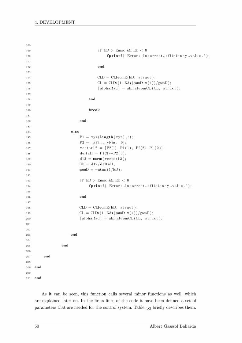
4. DEVELOPMENT

168

169 i f ED > Emax && ED < 0


171

172 end

173




177

178 end

179

180 break

181

182 end

183

184 else

185 P1 = xyz ( length ( xyz ) , : ) ;

186 P2 = [ xFin , yFin , 0 ] ;

187 vector12 = [ P2(1)−P1 ( 1 ) , P2(2)−P1 ( 2 ) ] ;

188 deltaH = P1(3)−P2 ( 3 ) ;

189 d12 = norm( vector12 ) ;



192

193 i f ED > Emax && ED < 0


195

196 end

197




201

202

203 end

204

205 end

206

207 end

208

209 end

210

211 end

As it can be seen, this function calls several minor functions as well, which

are explained later on. In the firsts lines of the code it have been defined a set of

parameters that are needed for the control system. Table 4.3 briefly describes them.


Parameter Description

h Current flight altitudeK1 Constant 1 used for the rolling controlK2 Constant 2 used for the rolling controlmuMax1 Maximum positive value of the roll angle during the main flightmuMin1 Maximum negative value of the roll angle during the main flightmuMax2 Maximum positive value of the roll angle in the approaching phasemuMin2 Maximum negative value of the roll angle in the approaching phaserA Vector pointing out the drone orientation in terms of yaw anglexyz 11×3 array that defines the approaching trajectoryxe Column vector with the x components of xyzye Column vector with the y components of xyzIAF Initial Approach Fix altitudeK3 Constant used for the control of the angle of attack

Table 4.3: Main parameters that are used by the control system.

4.3.1 Rolling control

Following it is explained how does the rolling control work, which is the part of

the controlFcn code comprised between lines 37 and 90. As it has already been

explained, the control system does not provide any roll angle until the global variable

logicalAlpha(2) is set to true, which is done when the air-relative flight path angle

reaches for first time a value of –π/4 and the drone has a normal flight attitude.

Afterwards, the system starts to control the roll angle as a function of the altitude,

the drone position and orientation and the location of the target landing point.

To do it, it uses the muControl function. As a function of the desired point

at which the drone is wanted to be directed (xD, yD) and the current position, it

is established the vector that the drone should follow, rpD. Then, the muControl

function establishes the roll angle that is needed to follow this vector. Following it

is shown the muControl function.

1 function [muRad ] = muControl ( rA , rpD , muMax, muMin, K)

2 % muControl r e tu rns the va lue o f the con t r o l parameter muRad as a

3 % func t i on o f the p o s i t i o n and o r i e n t a t i o n o f the a i r c r a f t .

4 % This func t i on uses one s i n g l e a l gor i thm . Fir s t , i t computes the ang l e

5 % between the vec t o r t ha t d e f i n e s the a i r c r a f t o r i e n t a t i on and the vec t o r

6 % from the a i r c r a f t l o c a t i o n to the de s i r ed po in t to f l y . Then , depending

7 % on the va l u e s o f t h a t ang l e s t h i s f unc t i on a s s i gn s a determined va lue to

8 % muRad.

9

10 [ angReal , angSmall ] = angleTwoVectors ( rpD , rA ) ;

11


13 case angSmall >= pi/2

14 i f angReal >= pi

15 muRad = muMax;


4. DEVELOPMENT

16

17 else

18 muRad = muMin ;

19

20 end

21

22 case angSmall < pi/2

23 i f angReal >= pi

24 muRad = K*angSmall ;

25

26 else

27 muRad = −K*angSmall ;

28

29 end

30

31 end

32

33 end

At the same time, the muControl function uses another secondary function as well,

angleTwoVectors:

1 function [ angleReal , ang leSmal l ] = angleTwoVectors (x , y )

2 % angleTwoVectors computes the e x i s t i n g ang l e between two g iven 2D

3 % vec t o r s .

4 % The output ang l e ang leRea l i s the one formed by vec t o r y wi th r e s p e c t to

5 % vec to r x , measured in the p o s i t i v e d i r e c t i o n . The output ang l e ang leSmal l

6 % i s the sma l l e s t one formed by both v e c t o r s and i s comprised between 0

7 % and p i .

8

9 x3D = [ x ( 1 ) , x ( 2 ) , 0 ] ;

10 y3D = [ y ( 1 ) , y ( 2 ) , 0 ] ;

11

12 angleSmal l = acos (dot (x , y )/ (norm( x )*norm( y ) ) ) ;

13 crossXY = cross (x3D , y3D ) ;

14

15 i f crossXY >= 0

16 angleReal = angleSmal l ;

17

18 else

19 angleReal = 2*pi−angleSmal l ;

20

21 end

22

23 end

The muControl function calls angleTwoVectors, which calculates the angle be-

tween rpD and rpA, the actual drone orientation. Concretely, it calculates the angle

that forms rA with respect rpD measured in the positive direction according to the

Earth-axes, and calls it angReal. The function also returns the smallest angle that

both vectors form, angSmall, so 0 < angSmall < π. Figure 4.11 shows graphically


these angles and the possible values that they can take, in an arbitrary position and

orientation of the drone.

Figure 4.11: Top view of the drone with an arbitrary position and orientation withthe values of angReal and angSmall in each zone.

In function of the value of these angles, the muControl function establishes the

proper roll angle to direct the drone to the rpD vector, following the next algorithm:

if angSmall ≥ π/2 then

if angReal ≥ π thenµ = µmax → µ > 0

elseµ = µmin → µ < 0

end

else

if angReal ≥ π thenµ = K ∗ angSmall→ µ > 0

elseµ = −K ∗ angSmall→ µ < 0

end

end

The roll angle is proportional to the angle between rA and rpD : the bigger is

this angle, the bigger will be the output roll angle. However, it has been fixed a

maximum and minimum values that can take µ in order to avoid too much abrupt

turns.

When the flight altitude is minor than IAF, the drone have to start the approach-

ing phase in order to land at the desired location with the correct orientation, and


4. DEVELOPMENT

the piloting rules change. In this way, the pathGen function generates an array that

define the path that the drone have to follow until it lands.

1 function [XYZ] = pathGen ( s t r u c t )

2 % pathGen genera t e s the path t ha t the drone shou ld f o l l ow in the l a s t

3 % phase o f the descen t in order to land at the de s i r ed po in t wi th the

4 % des i r ed o r i e n t a t i on . The path i s de f ined by 11 way−po in t s .5

6 Emax = s t r u c t .Emax ;

7 xFin = s t r u c t . xFin ;

8 yFin = s t r u c t . yFin ;

9 psiRW = s t r u c t . psiRW ;

10

11 EmaxLand = 0.8*Emax ;

12 angRW = psiRW*pi /180 ;

13 RWDir = [ cos (angRW) sin (angRW ) ] ;

14 xOrig in = xFin−2.5 e3*RWDir ( 1 ) ;

15 yOrig in = yFin−2.5 e3*RWDir ( 2 ) ;

16 zOr ig in = round(norm ( [ xOrigin−xFin , yOrigin−yFin ] ) / EmaxLand ) ;

17 R = 5e3 ;

18 n = 11 ;

19 xy = zeros (n , 2 ) ;

20 z = zeros (n , 1 ) ;

21

22 angP1 = −pi /2 ;

23 chiP1 = angRW+angP1 ;

24 xy ( 1 , : ) = [ xOrig in yOrig in ]+R* [ cos ( chiP1 ) sin ( chiP1 ) ] ;

25

26 for i =2:5

27 angPi = angP1+(i −1)*45*pi /180 ;

28 ch iP i = angRW+angPi ;

29 xy ( i , : ) = [ xOrig in yOrig in ]+R* [ cos ( ch iP i ) sin ( ch iP i ) ] ;

30

31 end

32 chiP5 = ch iP i ;

33

34 % (x−a)ˆ2+(y−b )ˆ2 = rˆ2

35 vect = [ xy(5 ,1)− xOrig in xy(5 ,2)− yOrig in ] ;

36 a = xOrig in+vect ( 1 ) / 2 ;

37 b = yOrig in+vect ( 2 ) / 2 ;

38 r = R/2 ;

39

40 for i =6:n

41 ch iP i = chiP5+(i −5)*30*pi /180 ;

42 xy ( i , 1 ) = a+r *cos ( ch iP i ) ;

43 xy ( i , 2 ) = b+r * sin ( ch iP i ) ;

44

45 end

46

47 distXY = zeros (1 , n−1);

48


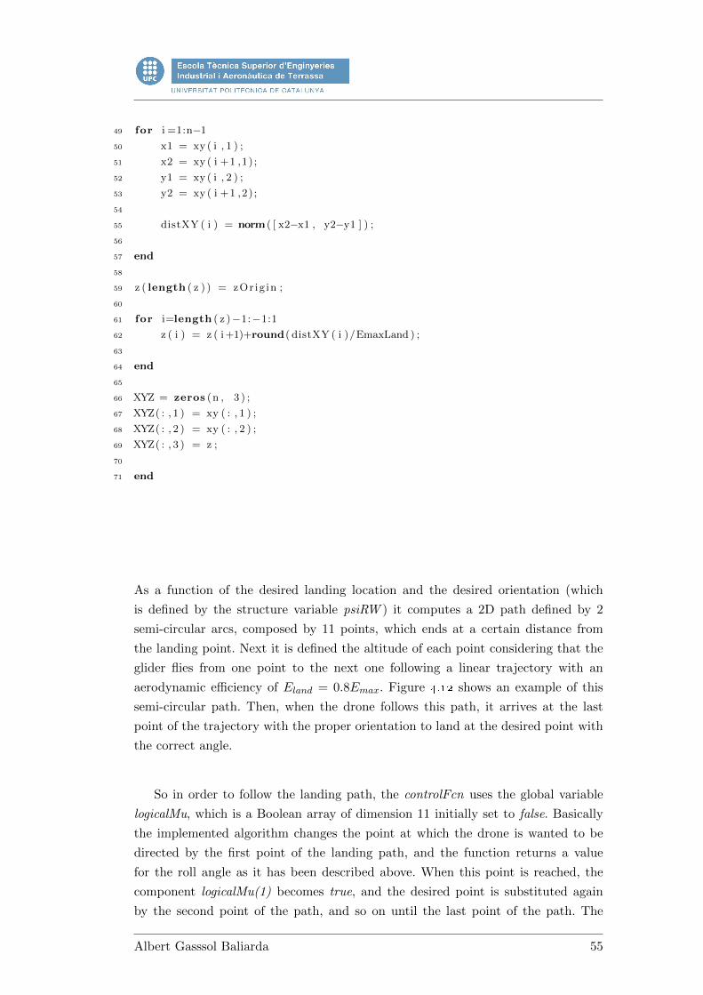
49 for i =1:n−1

50 x1 = xy ( i , 1 ) ;

51 x2 = xy ( i +1 ,1) ;

52 y1 = xy ( i , 2 ) ;

53 y2 = xy ( i +1 ,2) ;

54

55 distXY ( i ) = norm ( [ x2−x1 , y2−y1 ] ) ;

56

57 end

58

59 z ( length ( z ) ) = zOr ig in ;

60

61 for i=length ( z )−1:−1:1

62 z ( i ) = z ( i +1)+round( distXY ( i )/EmaxLand ) ;

63

64 end

65

66 XYZ = zeros (n , 3 ) ;

67 XYZ( : , 1 ) = xy ( : , 1 ) ;

68 XYZ( : , 2 ) = xy ( : , 2 ) ;

69 XYZ( : , 3 ) = z ;

70

71 end

As a function of the desired landing location and the desired orientation (which

is defined by the structure variable psiRW ) it computes a 2D path defined by 2

semi-circular arcs, composed by 11 points, which ends at a certain distance from

the landing point. Next it is defined the altitude of each point considering that the

glider flies from one point to the next one following a linear trajectory with an

aerodynamic efficiency of Eland = 0.8Emax. Figure 4.12 shows an example of this

semi-circular path. Then, when the drone follows this path, it arrives at the last

point of the trajectory with the proper orientation to land at the desired point with

the correct angle.

So in order to follow the landing path, the controlFcn uses the global variable

logicalMu, which is a Boolean array of dimension 11 initially set to false. Basically

the implemented algorithm changes the point at which the drone is wanted to be

directed by the first point of the landing path, and the function returns a value

for the roll angle as it has been described above. When this point is reached, the

component logicalMu(1) becomes true, and the desired point is substituted again

by the second point of the path, and so on until the last point of the path. The


4. DEVELOPMENT

Figure 4.12: Example of a standard path generated by pathGen, being in this casethe landing orientation ψ = 315°.

algorithm is the following:

for i = 2 : length(logicalMu) do

if logicalMu(i) = true thenDo nothing.

Go to the next loop iteration.

elsexD = xyz(i, 1)

yD = xyz(i, 2)

Compute µ.

CurrentDistance =√

(xD − x(1))2 + (yD − x(2))2

if CurrentDistance > DistanceHistorical thenlogicalMu(i) = true

elseDo nothing.

end

Leave loop.

end

DistanceHistorical = CurrentDistanceend

Finally, when the drone reaches the last point of the landing path, the location

where the drone is wanted to be directed is the landing location again, but now it

has the correct orientation to arrive at this point properly.

Summarizing all that, with controlling the roll angle, the control system directs

the drone to the landing position, whatever is its location. When the altitude is the

pre-established value IAF, the control system changes the piloting rules and orders


to follow a determined trajectory that allows the drone landing with the proper

conditions.

4.3.2 Control of the angle of attack

The control of the angle of attack is done in the part of the controlFcn code comprised

between lines 99 and 209. The angle of attack fixes the lift coefficient, so this control

parameter has a direct effect on the aerodynamic efficiency of the gliding. Thus, as

it has been seen in Chapter 3, for a given wing loading the aerodynamic efficiency

fixes the flight velocity as well, so with controlling the angle of attack actually there

are controlled both the flight endurance and the flight velocity.

In order to achieve an optimal gliding in terms of endurance and at the same time

ensure that wind velocities will not produce stall or any undesired effect, different

control patterns are established depending on the flight altitude:

� CL = CLopt when h > 12000 m.

� CL = CL|v=100 kt when 12000 m ≥ h > 7000 m.

� CL = CLopt when 7000 m ≥ h > IAF .

� Especial conditions during the approaching phase and landing.

When v = 100 kt for first time and the control system starts to give an angle

of attack in order to rotate the drone to get a normal flight altitude, the control

system looks for the angle of attack that produces CLopt, condition with which the

gliding endurance is maximized. However, this abrupt change in the lift coefficient

is too much in too few time, and the flight attitude is not stabilized. As a result, the

drone response is a phugoid oscillation (see Figure 4.13).

In order to avoid the phugoid oscillation, it is needed to make more progressive

the rise of the lift coefficient. This can be done with the following expression:

CL =CL1 (h− h2) + CL2 (h1 − h)

h1 − h2(4.32)

where in this case CL1 = 0, h1 = 20000 m and h2 = 12000 m. The value of CL2 is

calculated as follows:

CL2 = CLopt

(1−KγEmax − γ

γEmax

)(4.33)

which is an expression that instead of being directly CLopt, corrects the actual value

of CL making it approaching to CLopt. With these expressions it is obtained a bal-

anced value of CL, and then the drone response is as expected (see Figure 4.14).

When changing the CL pattern as a function of the flight altitude, similar

phugoids would appear in the drone flight as a consequence of this sudden change.


4. DEVELOPMENT

Figure 4.13: Phugoid oscillation as a result of a too much abrupt change of CL.

Figure 4.14: Smooth transition from the nose diving to a normal gliding attitude.

So, it is needed to create transition intervals in order to get always small changes in

the lift coefficient and make the flight as much continuous as possible. In this way,

the different altitude intervals that will have a different CL law at altitudes above

the IAF are:

� Interval 1 : 20000 m ≥ h > 13000 m. Starting with CL = 0, the lift coefficient

progressively becomes CLopt by using Equation (4.32) and Equation (4.33).

� Interval 2 : 13000 m ≥ h > 12000 m. This is a transition until the next interval,

and the transition is done by using Equation (4.32).


� Interval 3 : 12000 m ≥ h > 7000 m. This is the altitude range where it is

defined the wind field, and the gliding velocity must be high enough. So, here

the lift coefficient is:

CL =2mg cos γ

ρv2Sw(4.34)

where v is the desired flight velocity, in this case 100 kt.

� Interval 4 : 7000 m ≥ h > 6000 m. This is another transition zone, and the lift

coefficient is calculated by using again Equation (4.32).

� Interval 5 : 6000 m ≥ h > hIAF . In this interval the desired lift coefficient is

again CLopt, so it is calculated with Equation (4.33).

As it has been said, these patterns prioritize as the flight endurance as the flight

velocity, when it is needed. After calculating the lift coefficient in each case, the

alphaFromCL function –which could be considered as the inverse function of ae-

roCoeffs –calculates the angle of attack corresponding to the CL that is given as

input.

1 function [AoA] = alphaFromCL (CL, s t r u c t )

2 % alphaFromCL computes the ang l e o f a t t a c k corresponding to a determined

3 % CL, accord ing to the func t i on aeroCoe f f s . I t can be cons idered as

4 % the inv e r s e func t i on o f t h a t one .

5

6 AR = s t r u c t .AR;


8

9 CLmax = 1 . 3 3 3 1 ;

10 CLmin = −0.6799;

11 CL0 = 0 . 3 2 8 9 ;

12 Clalpha = 5 . 8 9 5 7 ; % [ radˆ−1]13 CLalpha = Clalpha /(1+ Clalpha /(pi*AR))*(1−1e−2); % [ radˆ−1]14 AoAPrima = (CL−CL0)/ CLalpha ;

15

16 i f CL == CL0

17 AoA = alpha0 ;

18

19 else

20 i f CL >= CLmin && CL <= CLmax

21 AoA = AoAPrima ;

22

23 else

24 fpr intf ( ’ Error : AoA not p o s s i b l e . ’ ) ;

25

26 end

27

28 end

29

30 end


4. DEVELOPMENT

When the drone is initiating the approaching phase and is going to the first

point of the path generated by pathGen, the control system calculates in real time

the distance in the horizontal plane between the actual position and the location

of this point, as well as the altitude difference. With these data, it establishes the

flight path angle that the drone should get in order to arrive at the desired point,

and then its corresponding CL by using the CLFromE function

1 function [CL] = CLFromE (E, s t r u c t )

2 % CLFromE computes the CL corresponding to a g iven aerodynamic e f f i c i e n c y

3 % and drag po la r . I t i s assummed g l i d i n g wi th sma l l f l i g h t path

4 % ang le .

5

6 K = s t r u c t .K;


8 CLmax = s t r u c t .CLmax;

9

10 % E = CL/CD = CL/(CD0+K*CLˆ2)

11 % CLˆ2−1/(E*K)*CL+CD0/K = 0

12 a = 1 ;

13 b = −1/(E*K) ;

14 c = CD0/K;

15 s o l 1 = (−b+sqrt (bˆ2−4*a*c ) )/ (2* a ) ;

16 s o l 2 = (−b−sqrt (bˆ2−4*a*c ) )/ (2* a ) ;

17

18 i f s o l 1 < 0 | | s o l 1 > CLmax

19 CL = s o l 2 ;

20

21 else

22 CL = s o l 1 ;

23

24 end

25

26 end

Finally, the control system calculates the lift coefficient and the angle of attack that

will be the output of the control system using an expression with the same structure

that (4.33):

CL = CLD

(1−KγD − γ

γD

)(4.35)

Afterwards arriving at the first point of the approaching path, it is used a similar


algorithm of which has been used for the µ control, which is the following:

for i = 2 : length(logicalMu) do

if logicalMu(i) = true thenDo nothing.

Go to the next loop iteration.

elseCalculate distance between Pi−1 and Pi.

Calculate altitude difference between Pi−1 and Pi.

Calculate γD and CLD.

CL = CLD

(1−K γD−γ

γD

)end

Leave loop.

end

In the end, when it has been reached the last point of the approaching path, it

is done the same process being in this case the desired point the landing position.

4.4 Results

With the established model and the control system acting on it, running the whole

simulation gives the following results:

Figure 4.15: 3D plot of the whole trajectory followed by the drone.


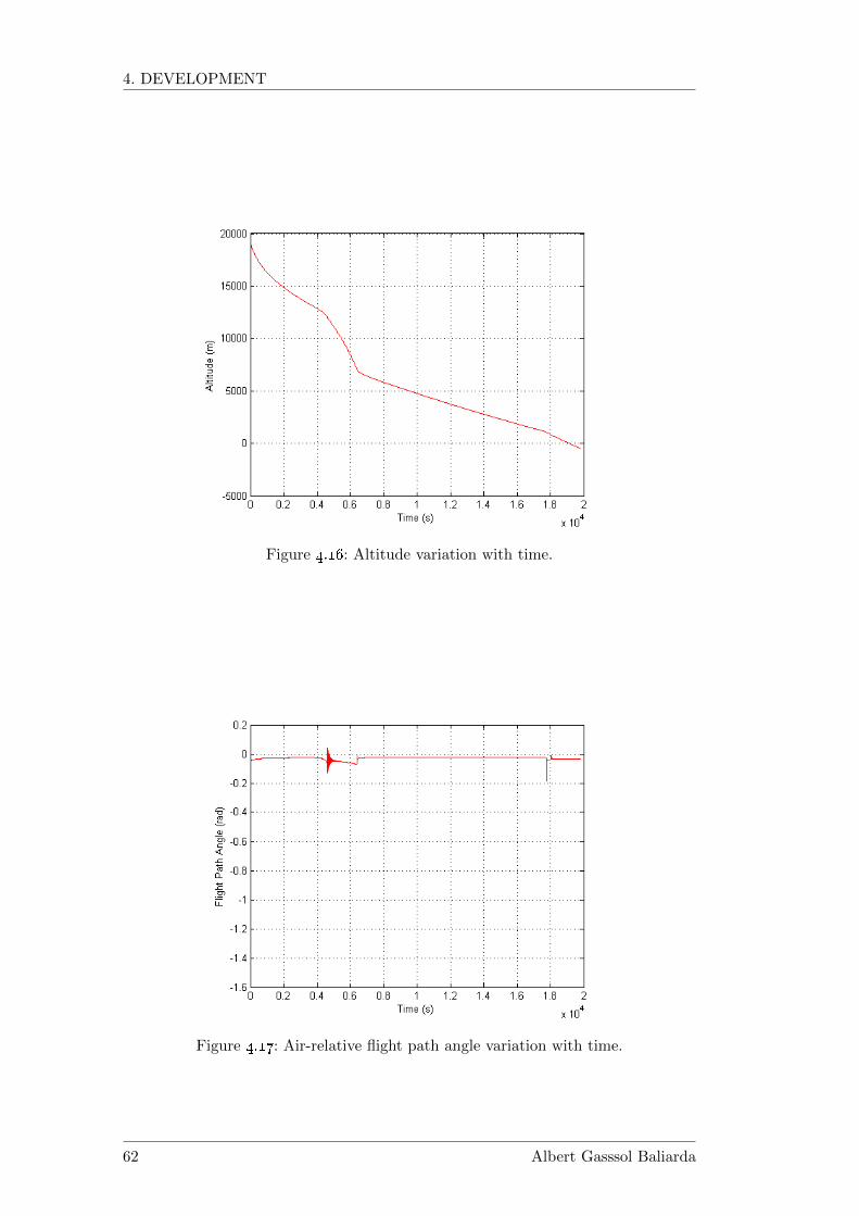
4. DEVELOPMENT

Figure 4.16: Altitude variation with time.

Figure 4.17: Air-relative flight path angle variation with time.


Figure 4.18: Horizontal distance from the landing location at each moment.

Figure 4.19: Variation of the aerodynamic velocity with time.


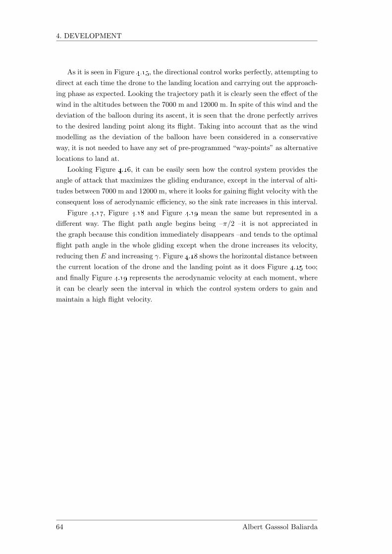
4. DEVELOPMENT

As it is seen in Figure 4.15, the directional control works perfectly, attempting to

direct at each time the drone to the landing location and carrying out the approach-

ing phase as expected. Looking the trajectory path it is clearly seen the effect of the

wind in the altitudes between the 7000 m and 12000 m. In spite of this wind and the

deviation of the balloon during its ascent, it is seen that the drone perfectly arrives

to the desired landing point along its flight. Taking into account that as the wind

modelling as the deviation of the balloon have been considered in a conservative

way, it is not needed to have any set of pre-programmed “way-points” as alternative

locations to land at.

Looking Figure 4.16, it can be easily seen how the control system provides the

angle of attack that maximizes the gliding endurance, except in the interval of alti-

tudes between 7000 m and 12000 m, where it looks for gaining flight velocity with the

consequent loss of aerodynamic efficiency, so the sink rate increases in this interval.

Figure 4.17, Figure 4.18 and Figure 4.19 mean the same but represented in a

different way. The flight path angle begins being –π/2 –it is not appreciated in

the graph because this condition immediately disappears –and tends to the optimal

flight path angle in the whole gliding except when the drone increases its velocity,

reducing then E and increasing γ. Figure 4.18 shows the horizontal distance between

the current location of the drone and the landing point as it does Figure 4.15 too;

and finally Figure 4.19 represents the aerodynamic velocity at each moment, where

it can be clearly seen the interval in which the control system orders to gain and

maintain a high flight velocity.


Chapter 5

Summary of results

5.1 Economic aspects

As the study of the economic feasibility of any lucrative project based on this study

is not amongst the own objectives of this study, this section just attempts to gather

the costs derived from this study together with the costs of launching the weather

balloon and the drone one time, without any lucrative interest.

In this way, the costs which have to be taken into account are:

� Products costs.

� Shipping costs.

� Costs derived from the study.

� Contingencies.

Products costs include on the one hand the Discus 2b drone and the servos

which should be installed to control it, and on the other hand the 2000 g weather

balloon and the helium with which it is filled. The drone model is taken from the

Canadian Icare RC, as it is explained in Chapter 3. The servos –which according

to the drone manufacturerar are 4 –are taken from the US Savox and, even though

they have not been determined in this study because this requires a rigid solid-like

analysis (see Chapter 4), their possible cost is estimated. The weather balloon is

taken from the Indian company PAWAN [24], and the helium gas costs anywhere

about 21 ¿/m3 [25]. Knowing it, the cost of each product that is needed to be bought

can be seen in Table 5.1:

Regarding the costs derived from this theoretical study of viability, they are the

MATLAB license and the human resources costs. The MATLAB Student License

can be purchased at its own portal web https://es.mathworks.com/store/. The

study consists of 600 hours of dedication, and the price of one hour of dedication of

the aeronautical engineer has been established on 45 ¿.


https://es.mathworks.com/store/

5. SUMMARY OF RESULTS

Product Cost per unit

PAWAN weather balloon (with shipping costs) 225,00 USD/uDiscus 2b scale model 1829 CAD/uHelium 20,95 ¿/m3

Savox SH-1257MG 64,99 USD/u

Table 5.1: List of products with its unit prices.

Shipping costs relating to the Discus 2b scale model and the Savox SH-1257MG

are taken into account by asking to the shipping company FedEx how much would

cost shipping a package of 7 kg (the drone weighs 6.8 kg) from Canada to Spain

and another one with the 4 servos from US to Spain, and this costs are estimated

in 315 ¿and 84.63 ¿, respectively.

In addition, it is added a percentage of the product costs (including its ship-

ping costs) to include any contingency that is not considered. This percentage is

established as the 10% of these costs. These contingencies take into account the

continuous change in the exchange rate as well. Since the products are imported

from several countries, they are bought using different currencies, and it should be

considered that when boughting the products, the exchange rate could be different

of the employed at the moment of calculating the budget, and so the total price.

Table 5.2 shows the exchange rate employed in this budget.

Currency Equivalenence in ¿

1 USD 0,9121 ¿

1 CAD 0,7339 ¿

Table 5.2: Exchange rate used in this budget.

Considering all that, the final budget is:

Budget

Products total costs 2026,82 ¿

Shipping costs 399,63 ¿

Costs of the study 27500,00 ¿

Contingencies 242,64 ¿

Budget 30169,09 ¿

Table 5.3: Budget of the project.

All these costs can be better seen and itemised in more detail in the budget of

this study.


5.2 Environmental study and implications

In this section it is analysed the environmental impact that this project has. It is

studied the implications of sending a relative heavy payload to a high altitude and

what does the usage of a non-propelled drone like the Discus 2b scale model mean,

as well as the environmental wastes that are produced.

5.2.1 Drone environmental issues

In this aspect, this one is a very sustainable project: the drone is lifted up to the

target altitude taking advantage of the Archimedes’ principle, with clean and natural

energy, and afterwards it goes back to the desired location without any propulsion

system. Thus, the only things that are needed to provide the necessary energy are,

on the one hand, a determined quantity of helium to fill up the weather balloon and

lift its payload (see Chapter 4), and on the other hand, a battery which is placed

onto the drone and which is in charge of supplying both the systems on board and

the drone’s servos that move the control surfaces. According to its manufacturer,

the requested servos are 4 [13]. So in addition with the fact that the drone is of large

dimensions, the battery would be of relative high power.

Regarding the materials which the drone model is composed of, they are basically

hardened steel, carbon fibre and polyurethane. All these materials can be reused for

different applications and can be easily recycled [26, 27, 28]. In addition, when they

are recycled the manufacturing process requires a minor quantity of energy than

when it uses new materials.

5.2.2 Environmental wastes

Probably this is the less eco-friendly aspect of this project: after reaching the desired

altitude leaving its payload, the latex balloon bursts and drops to the Earth surface,

and it becomes part of the rubbish of the planet. Weather balloons are typically

constructed using natural rubber latex with a set of modifications that make it

more durable and improve its protection against biological degradation.

O. O’Shea, M.Hamann, W.Smith et al. carried out a study about the pollution

associated with weather balloons [29]. This study –done in the Great Barrier Reef

World Heritage Area, although its results are extrapolable –shows that weather

balloon wastes are very likely to end up in marine environments, where they are

especially harmful. While latex degrade faster than many plastic polymers, in marine

environments it persists for periods of time long enough to pose significant threats

to marine animals.

The animals confuse these plastic wastes with food, so they can choke. The plastic

wastes can also block or perforate their digestive tract or cause digestive dilution,

causing them suffering and possible death. Furthermore, due to the several marine



currents that take place in the oceans the latex wastes are very likely to be dragged

till the coast, resulting dangerous for the shore taxa as well.

5.3 Security aspects

The security considerations that have to be taken into account in this project are

related as with the weather balloon launching as with the usage of the drone. Both

aspects are regulated by the states with a legal framework, although this legal frame-

work may vary depending on each state.

5.3.1 Weather balloon-related security aspects

Regarding the security considerations about the launching of a weather balloon at

high altitudes, all the security measures that should be taken are described in the

Air Traffic Regulations – Appendix S: Ummaned free balloons [30]. These regulations

establish that it is necessary to obtain a permission from AESA in order to launch

any balloon, and that it is not permitted the launching of any balloon which payload

could mean a danger to the other people. So, it will be needed a parachute system

attached to the drone that brakes it in case of any failure causes the balloon’s payload

drop. Furthermore, it cannot fly at heights minors than 300 m above populated zones.

According to the payload that the weather balloon of this project would carry,

this balloon is classified as a heavy balloon by the regulations. It supposes, amongst

other things, that the balloon-payload assemble must have two independent systems

which allows interrupting the flight if it were necessary for any case. These cases

in which it is necessary to interrupt the flight of the balloon are properly described

in the already menctioned Air Traffic Regulations – Appendix S: Ummaned free

balloons, as well as the rest of security measures and legal procedures to launch a

balloon at high altitudes.

5.3.2 Drone-related security aspects

Regarding the drone, as it is mentioned in Chapter 2, at this moment it exists a

temporal framework that regulates all the activities that are related with drones.

It establishes a set of limitations in its usage and security measures. However, this

regulation is thought for RPA and not for autonomous aircraft, being these ones out

of the Spanish legal framework, so it would not be possible to carry out a launching

of the drone that this project is about so far (at least at this state). This is due to

autonomous drones present lots of logistical troubles with air traffic and the current

regulations of the aeronautical world, so as it is menctioned in Chapter 2 they are

unsuitable at the moment.

But supposing that it is possible to carry out a flight anywhere where it does not

exist any interference with air traffic or in another state, assuming that the control


system has been properly developed and it does not exist any situation that could

occur causing confusion to it (it is very important to be sure about this), the main

security measures that should be taken are related with any electronic failure that

could occur or any inaccuracy of the sensors that causes a malfunction of the control

system.

5.4 Temporal aspects and planning

Since this study –under the point of view it has been carried out –concludes that the

programmed piloting rules are valid to make a glider with the proper specifications

go back from the stratosphere, next steps of this medium-term project (which would

finish with a real launching of a first prototype) are further analyses that permit

accurate which should be the optimal design of the employed drone. At the same

time, a better knowledge of the drone specifications opens the possibility to carry

out more complex studies about its behaviour in flight.

So, following it is done a proposal of the next steps that should be carried out:

� Design of a drone model specifically to carry out this kind of mission.

� Obtaining all the requested physical parameters that are needed for its analyses

and control.

� Development of a rigid solid dynamic model.

� Adapting the current control system to the new dynamic model.

� Iteration process, changing any design parameter in order to improve and

optimize the flight performances and stability.

� Construction of a prototype and first flight.

5.4.1 List of tasks

The main tasks to carry out in the next phases of the project are:

A – Design of a drone model specifically to carry out this kind of mission.

A.1 – Aerodynamic design: wing, tail and control surfaces analyses.

A.2 – Materials selection and structural design.

A.3 – Construction with any CAD software.

B – Obtaining all the requested physical parameters that are needed for its analyses

and control.

B.1 – Analytical.

B.2 – Numerical simulation.



B.3 – Experimental.

C – Development of a rigid solid dynamic model.

C.1 – Implementation.

C.2 – Verification.

D – Adapting the current control system to the new dynamic model.

D.1 – Static stability analysis.

D.2 – Dynamic stability analysis.

D.3 – Modification of the current control patterns and adaptation to the new

rigid solid model.

E – Iteration process, changing any design parameter in order to improve and op-

timize the flight performances and stability.

F – Construction of a prototype and first flight.

F.1 – Construction of a prototype.

F.2 – Equipping the prototype with all the systems and instrumentation.

F.3 – Electronics setting up.

5.5 Conclusions and recommendations

This study is about the technical viability of a non-propelled drone to go back in

an autonomous way from the stratosphere to the pre-programmed base, returning

a determined payload. The drone is taken at an altitude of 20000 m by means of

a non-recoverable weather balloon, and then it initiates the descent flight. During

the descent flight, the control system is in charge of providing at each moment the

outputs that control the drone in such a way that it goes back to the base doing a

high endurance gliding.

The result of this study, which has to be considered valid only under the con-

siderations and hypotheses that have been done, is that this concept is possible to

carry out if the design of the drone and its specifications are appropriate enough.

These conditions are basically that the drone needs to have a relative high wing

loading, because this condition directly increases its flight velocity, and the drone

needs to get high flight velocities in order to overcome the strong wind speeds that

take place at the high altitudes where the drone shall flight at. This specification is

the most important one that the drone that this study is about needs getting.

A possible improvement could be to evaluate if it is possible to develop the

mission that this study deals with using a lighter drone. Even though a relative

high wing loading (which means a relative heavy drone) is requested, this fact is


completely opposed with raising the drone with a weather balloon. The actual weight

is considerable if it must be raised with a balloon, so any possible reduction of the

weight that could be done in further studies would be of significant importance.

To arrive at the conclusion that the project would be theoretically viable from

a technical point of view, it has been developed a physical model that describes, on

the one hand, the atmosphere and the physical phenomena that take place in it after

having studied them, and on the other hand, the drone dynamics, assuming it as a

point-mass. Then, it has been developed the control system, which acting over the

control parameters of the drone –the roll angle and the angle of attack –is in charge

of returning it to the base.

It is important to point out that the drone is always capable of returning to

the base, even being conservative with the analysis as it is explained in the end of

Chapter 4. Due to this reason, it has not been programmed any set of alternative

landing points, as it is menctioned in Chapter 1, in case that landing at the base was

not possible. However, this could be included in the next phases of the project that

have been established in Section 5.4, considering that in a real flight it can occur

much more situations and random atmospheric phenomena that what is predicted

by a statistical wind model.

Nevertheless, as it has been a first study of technical viability, the developed

model is a simple one, due to the data that would be needed in order to do more

complex analyses (i.e., stability analysis with a rigid body modelling) is not known

at this point as well. So, the result of this study does not mean that next step is

launching the balloon with the drone and that all will work fine, but it means that it

is worth to continue this project with the next phases planned in Section 5.4, which

include design and more advanced analyses.


Bibliography

[1] R Austin. Unmanned aircraft systems. Ed. by Ian Moir, Allan Seabridge, and Roy

Langton. Vol. 54. Wiley, 2009. isbn: 9780470664797. doi: 10.1002/9780470664797.

[2] OACI. Circular 328, Sistemas de aeronaves no tripuladas ( UAS ). International

Civil Aviation Organization, 2011. isbn: 9789292318093.

[3] Wikipedia contributors. Unmanned aerial vehicle. 2015. url: http://en.wikipedia.

org/w/index.php?title=Unmanned\_aerial\_vehicle\&oldid=649546505 (vis-

ited on 03/04/2015).

[4] Antonio Baquero and Carles Planas. Drones, la ultima revolucion militar. Barcelona,

Mar. 2015.

[5] General Atomics. MQ-9 Reaper. url: http://media.ga.com/image-library/

unmanned-aircraft-systems/aircraft-platforms/ (visited on 03/10/2015).

[6] Jefatura del Estado. Boletın oficial del estado. Real Decreto-ley 8/2014. 2014.

[7] Stelio Frati. The glider. 1946. url: http://hdl.handle.net/2060/19930094860.

[8] Wikipedia contributors. Polar curve (aerodynamics). 2015. url: http://en.wikipedia.

org/w/index.php?title=Polar\_curve\_(aerodynamics)\&oldid=603239473.

[9] Robert G. Fleagle and Joost A. Businger. An introduction to atmospheric physics.

Ed. by J. Van Mieghem and Anton L. Hales. 2nd ed. Seatle: Academic Press, 1980.

isbn: 0122603559.

[10] Wikipedia contributors. Jet stream. 2015. url: http://en.wikipedia.org/w/

index.php?title=Jet\_stream\&oldid=651091680 (visited on 03/16/2015).

[11] National Weather Service. The Jet Stream. 2011. url: http://www.srh.noaa.gov/

jetstream//global/jet.htm (visited on 03/16/2015).

[12] M Sadraey. Aircraft performance analysis. Wiley Publications, 2012.

[13] Icare RC. Scale gliders ¿ 4m. url: http://www.icare-rc.com/scale\_glider\

_over4m.htm (visited on 03/30/2015).

[14] Schempp-Hirth. Discus 2a/2b. url: http://www.schempp-hirth.com/ (visited on

04/30/2015).

[15] HQ 2.5/12 AIRFOIL. url: NoTithttp://airfoiltools.com/airfoil/details?

airfoil=hq2512-ille (visited on 04/30/2015).


http://dx.doi.org/10.1002/9780470664797

http://en.wikipedia.org/w/index.php?title=Unmanned\_aerial\_vehicle\&oldid=649546505

http://en.wikipedia.org/w/index.php?title=Unmanned\_aerial\_vehicle\&oldid=649546505

http://media.ga.com/image-library/unmanned-aircraft-systems/aircraft-platforms/

http://media.ga.com/image-library/unmanned-aircraft-systems/aircraft-platforms/

http://hdl.handle.net/2060/19930094860

http://en.wikipedia.org/w/index.php?title=Polar\_curve\_(aerodynamics)\&oldid=603239473

http://en.wikipedia.org/w/index.php?title=Polar\_curve\_(aerodynamics)\&oldid=603239473

http://en.wikipedia.org/w/index.php?title=Jet\_stream\&oldid=651091680

http://en.wikipedia.org/w/index.php?title=Jet\_stream\&oldid=651091680

http://www.srh.noaa.gov/jetstream//global/jet.htm

http://www.srh.noaa.gov/jetstream//global/jet.htm

http://www.icare-rc.com/scale\_glider\_over4m.htm

http://www.icare-rc.com/scale\_glider\_over4m.htm

http://www.schempp-hirth.com/

No Tithttp://airfoiltools.com/airfoil/details?airfoil=hq2512-ille

No Tithttp://airfoiltools.com/airfoil/details?airfoil=hq2512-ille

BIBLIOGRAPHY

[16] Jose Meseguer Ruiz and Angel Sanz Andres. Aerodinamica basica. 2nd ed. Madrid:

Garceta, 2011. isbn: 978-84-9281-271-4.

[17] Colegio Mayor Universitario Chaminade. CHATSAT: sondas estratosfericas caseras.

2011. url: http://chasat.blogspot.com.es/p/construye-tu-propia-sonda-

casera.html (visited on 05/07/2015).

[18] Nancy Hall. Drag of a sphere. 2015. url: https://www.grc.nasa.gov/www/k-

12/airplane/dragsphere.html (visited on 05/19/2015).

[19] R.S. Subramanian. “Drag on spherical particles and steady settling velocities”. In:

(1978), pp. 1–3. url: http : / / web2 . clarkson . edu / projects / subramanian /

ch301/notes/dragsphere.pdf.

[20] Hwoyee. Hwoyee meteorological balloons. 2013. url: http://www.hwoyee.com/

images.aspx?fatherId=11010101\&msId=1101010101 (visited on 05/05/2015).

[21] Yiyuan J. Zhao. “Optimal patterns of glider dynamic soaring”. In: Optimal Control

Applications and Methods 25.December 2003 (2004), pp. 67–89. issn: 01432087. doi:

10.1002/oca.739.

[22] M.A. Gomez Tierno. Tema 2: Sistemas basicos de referencia. Madrid.

[23] Mark Voskuijl. Flight and Orbital Mechanics - Equations of motion. 2012.

[24] PAWAN. Weather balloons. 2012. url: http://www.pawanexport.com/meteorological-

weather-balloons.shtml (visited on 05/25/2015).

[25] High Altitude Science. Helium. 2015. url: http://www.highaltitudescience.

com/pages/helium (visited on 05/25/2015).

[26] Wikipedia contributors. Ferrous metal recycling. 2015. url: http://en.wikipedia.

org/w/index.php?title=Ferrous\_metal\_recycling\&oldid=658684649

(visited on 05/25/2015).

[27] American Chemestry Council. Polyurethane recycling. 2015. url: http://polyurethane.

americanchemistry.com/Sustainability/Recycling (visited on 05/25/2015).

[28] Gregory Polek. Composites Go Green Through Recycling. 2012. url: http://www.

ainonline . com / aviation - news / aerospace / 2012 - 11 - 05 / composites - go -

green-through-recycling (visited on 05/25/2015).

[29] Owen R. O’Shea et al. “Predictable pollution: An assessment of weather balloons

and associated impacts on the marine environment - An example for the Great

Barrier Reef, Australia”. In: Marine Pollution Bulletin 79 (2014), pp. 61–68. issn:

0025326X. doi: 10.1016/j.marpolbul.2013.12.047. url: http://dx.doi.org/

10.1016/j.marpolbul.2013.12.047.

[30] Jefatura del Estado. Real Decreto 57/2002, Apendice S. Globos libres no tripulados.

2014.


http://chasat.blogspot.com.es/p/construye-tu-propia-sonda-casera.html

http://chasat.blogspot.com.es/p/construye-tu-propia-sonda-casera.html

https://www.grc.nasa.gov/www/k-12/airplane/dragsphere.html

https://www.grc.nasa.gov/www/k-12/airplane/dragsphere.html

http://web2.clarkson.edu/projects/subramanian/ch301/notes/dragsphere.pdf

http://web2.clarkson.edu/projects/subramanian/ch301/notes/dragsphere.pdf

http://www.hwoyee.com/images.aspx?fatherId=11010101\&msId=1101010101

http://www.hwoyee.com/images.aspx?fatherId=11010101\&msId=1101010101

http://dx.doi.org/10.1002/oca.739

http://www.pawanexport.com/meteorological-weather-balloons.shtml

http://www.pawanexport.com/meteorological-weather-balloons.shtml

http://www.highaltitudescience.com/pages/helium

http://www.highaltitudescience.com/pages/helium

http://en.wikipedia.org/w/index.php?title=Ferrous\_metal\_recycling\&oldid=658684649

http://en.wikipedia.org/w/index.php?title=Ferrous\_metal\_recycling\&oldid=658684649

http://polyurethane.americanchemistry.com/Sustainability/Recycling

http://polyurethane.americanchemistry.com/Sustainability/Recycling

http://www.ainonline.com/aviation-news/aerospace/2012-11-05/composites-go-green-through-recycling



http://dx.doi.org/10.1016/j.marpolbul.2013.12.047



study of the viability of a glider drone for the return of ... · unmanned aerial vehicles (uav),...

Documents