study on ozone change over the tibetan plateau2 zhou xiuji, li weiliang, chen longxun and liu yu 129...

NO.2 ZHOU Xiuji, LI Weiliang, CHEN Longxun and LIU Yu 129

Study on Ozone Change over the Tibetan Plateau

ZHOU Xiuji (��

), LI Weiliang ( �� ), CHEN Longxun( �� ), and LIU Yu ( �� )

Chinese Academy of Meteorological Sciences, Beijing 100081

(Received May 9, 2006)

ABSTRACT

This paper reviewed the main results with respect to the discovery of low center of total column ozone(TCO) over the Tibetan Plateau (TP) in summer, and its formation mechanism. Some important advancesare summarized as follows: The fact is discovered that there is a TCO low center over the TP in summer,and the features of the background circulation over the TP are analyzed; it is confirmed that the TP is apathway of mass exchange between the troposphere and stratosphere, and it influences the TCO low centerover the TP in summer; models reproduce the TCO low center over the TP in summer, and the formationmechanism is explored; in addition, the analyses and diagnoses of the observation data indicate that notonly there is the TCO low center over the TP in summer, but also TCO decrease trend over the TP is oneof the strong centers of TCO decrease trend in the same latitude; finally, the model predicts the future TCOchange over the TP.

Key words: the Tibetan Plateau (TP), the TP ozone valley, pathway, total column ozone (TCO) decrease

trend

1. Introduction

Ozone is an important trace gas in the atmo-

sphere, and is paid more attention due to the discov-

ery of the Antarctic “ozone hole”. In addition, tropo-

spheric ozone and the effects of ozone on human being,

ecosphere, and climate are also drawn more attention.

In the last decade, facts are confirmed by many ob-

servations that anthropogenic activities result in the

significant ozone changes in the stratosphere and tro-

posphere (Bojkov, 1994). In China, Wei et al. (1994)

analyzed the total column ozone (TCO) in Beijing and

Kunming from DOBSON instruments since 1979, and

their results showed that the TCO in both sites contin-

uously decreases, and the decrease became more ob-

vious after 1991. In order to realize roundly ozone

changes over China during the last decade, we focused

the above issues, and paid special attention to the TP.

In this paper, we review the results with respect to the

ozone over the TP.

2. The TCO low center over the TP in

summer

The TCO from TOMS (Total Ozone Meteorolog-

ical Satellite) over Nimbus satellite is widely used to

research ozone changes and its spatiotemporal distri-

bution. When Reiter and Gao (1982) researched the

South High movement and heating field over the TP,

they used the TOMS data from March to April in

1979 and gave some figures related to weather pro-

cess. These figures showed that there occurs low TCO

over the TP as the South High moves to the TP in the

middle April.

By using TOMS data from 1979 to 1991, Zhou

et al. (1995) gave the distribution of monthly mean

ozone over China. Figure 1 shows the TCO distribu-

tion in January, whose isolines roughly parallels with

latitude. But in June there appears an obvious

TCO low center over the TP, which maintains until

Fig.1. Distribution of monthly averaged total column

ozone in January (1979-1991) (unit: DU).

130 ACTA METEOROLOGICA SINICA VOL.20

September (Fig.2). Meanwhile, there is a TCO high

center over Northeast China. The TCO low center

over the TP disappears after October. Compared

the TCO over the TP with the counterpart over East

China at the same latitude, it is found that the TCO

difference between both sites is less than 3% in winter

and spring, but about 10% in summer with maximum

of 11% in June (Fig.3). Therefore, some physical and

chemical processes result in the TCO fall over the TP

in summer. The TCO fall is less than Antarctic “ozone

hole”. The TCO low center over the TP in summer

is called “TP ozone valley”.

By using the same TOMS data, Zou (1996) and

Zou et al. (1998) gave the global climate average of the

TCO in different seasons, which further confirmed that

the ozone valley not only occurs over the TP (com-

pared with the TCO of the same latitude, it lowers

more than 30 DU) but also over the Rocky Mountains

(lowers by about 20 DU).

Fig.2. Distribution of monthly averaged total column

ozone in July (1979-1991) (unit: DU).

Fig.3. Difference of total column ozone between the

Tibetan Plateau and east part of China at the same

latitude.

3. Role of seasonal variations of wind field on

the ozone over the TP and its surroundings

Zhou et al. (1995) presumed that based on previ-

ous researches on the meteorology over the TP, South

Asian high caused by thermodynamic role controls at-

mosphere from 500 to 100 hPa over the TP, in which

convective activities occur largely. Synthesis meteo-

rology experiments over the TP indicated that the TP

is mostly a convergence area in summer. They specu-

lated that the TP is an important pathway in summer

by which the air in low troposphere can be transported

into the stratosphere. The pollutants from the TP

surroundings of several hundreds kilometers may be

converged to the TP in summer, and transported into

the stratosphere, then diverged to the surroundings.

Thus, low content ozone and high content pollutants

from the troposphere are transported into the strato-

sphere so that they bring about abnormal TCO fall by

some physical and chemical process. In order to verify

the above presumption, Bian et al. (1997) analyzed

seasonal characters of wind field over the TP and its

surroundings with ECMWF reanalysis data of 7 lev-

els from 1980 to 1989 and sounding data of 1995 over

the southeast of TP. The results showed that in winter

horizontal wind field is a shallow cold high near surface

over the TP (Fig.4), and western wind in the middle

and high troposphere. During the transit period from

winter to summer, southern wind component over the

TP expands upward and northward with seasonal vari-

ations. The convergence from the TP surroundings to

the TP also expands upward and northward. In July

and August, the low and middle troposphere over the

TP becomes a strong convergence area.

In winter, the vertical wind field over the TP is

mostly falling except the northwest part of the TP

(Fig.5). In spring (April), the ascending flow occurred

first in low troposphere over the southeast part of the

TP, then gradually expands upward and to its sur-

roundings. In summer, there becomes the ascending

flow in the whole troposphere over the TP, and the

TP and Bay of Bengal together form a large region

of strong ascending flow that is upward part of mon-

soon vertical circulation. Since May the currents from

south, east, and north began to flow to the TP.


Fig.4. Averaged geopotential height at 100 hPa (a) and streamline field at 850 hPa (b) in January (1980-1989).

In June, the strong ascending flow occurred over the

west part of TP (Fig.6). The ascending flow is the

strongest in July and August, with the maximum to

100 hPa. This is because the TP is a heating source

in summer.

This is also confirmed by results of 2-D global

dynamical-radiative-chemical coupled model by Fu et

al. (1997, figure omitted). The model result showed

that the upward flow of latitudinal circulation over the

TP and its surroundings could reach 20 km.

In a word, there becomes the ascending flow in

the whole troposphere over the TP in summer, which

climbs up the TP from TP surroundings, and reaches

the upper troposphere and lower stratosphere where

the strong South High controls, then diverges into the

surroundings. In addition, convections over the TP

are also active in summer. These features of benefit

to the convergence of mass and pollutants from the

TP surroundings, which reach lower stratosphere over

the TP and diverge into the surroundings. This is a

favorable circulation background under the condition

of which the TP ozone valley occurs.

4. Mass exchange between stratosphere and

troposphere over the TP and its surround-

ings

Based on the favorable circulation background,

Zhou et al. (1995) proposed that the TP is an im-

portant pathway in summer by which the air in low

troposphere can be transported into the strato-

sphere. In order to verify this view, Cong et al. (2001)


Fig.5. Averaged ω at 300 hPa (a) and 500 hPa (b) in January (1980-1989) (unit: 10−6 hPa s−1).

calculated mass exchange cross the tropopause over

the TP and its surroundings by Wei (1987)’s way with

NCEP reanalysis daily data (1978-1996). The results

indicated that in summer strong mass exchanges from

troposphere to stratosphere occur over the TP, its

southeast part and the north part of Bay of Bengal.

4.1 Nineteen-yr mean seasonal variation fea-

ture of the cross-tropopause mass exchange

(CTME) over the TP and its surroundings

The distribution of the monthly mean CTME over

the TP and its surroundings are shown in Fig.7a.

From Fig.7a, it is found that in January except for the

weak mass transport from troposphere to stratosphere

(TTS) in the northwest part of the TP, the Hanshui

valley and the Poyang Lake, the transport from strato-

sphere to troposphere (TST) appears in the south and

east of the TP with a large value center, where there

is descending flow center. The TST weakens during

March and April. In May, the TTS is found in the

southeast of the TP. Until June, the TTS in the east

of TP becomes stronger and moves northward to the

north of the TP when it becomes quite stable. The

cross-tropospause mass exchange in summer is very

different from that in winter. In summer (Fig.7b), the

area of south of 40◦N in Asia is covered by the TTS


Fig.6. Averaged ω at 300 hPa (a) and 500 hPa (b) in July (1980-1989) (unit: 10−6 hPa s−1).

Fig.7. Nineteen-yr averaged mass exchange flux across the tropopause in winter (a) and summer(b) (unit: 10−3 kg m−2s−1).


with two high centers located at the north of Bay of

Bengal and southeast of TP.

4.2 Nineteen-yr mean seasonal variation fea-

ture of net mass exchange flux across

tropopause over the TP and its surround-

ings

The monthly variation feature of the mass bud-

get across tropopause over the TP and its surround-

ings (15◦-40◦N, 80◦-110◦E) is shown in Fig.8. The

TST weakens step by step from January to April.

In May, the TST and TTS reach the balance basi-

cally. From June the net cross-tropopause mass ex-

change appears, and the net TTS gradually becomes

stronger. Until mid-summer (July and August) the

net TTS reaches the maximum. In September the

TTS becomes weaker, and the TST and TTS reach

the balance again in October. The net TST occurs

into the troposphere in November and December.

4.3 The relationship between aerosol, ozone of

100 hPa, and the cross-tropopause mass

over the TP and its surroundings

In the study of the aerosol distribution, Li and

Yu (2001) pointed out that the maximal aerosol ap-

pears at 100 hPa over the TP in summer. This level

is approximately the height of the tropopause. Cong

et al. (2001) found that the aerosol maximum also

occurs in Bay of Bengal and southeast of the TP in

July. And they calculated the annual variation of area

average aerosol and ozone at 100 hPa and the correla-

tion between aerosol, ozone, and the cross-tropopause

mass. The results indicated that there was a positive

correlation between the cross-tropopause mass and the

Fig.8. Monthly variation of 19-yr averaged mass ex-

change flux across the tropopause over a region (15◦-

40◦ N, 80◦-115◦E) (unit: kg month−1).

aerosol concentration of 100 hPa; and there was a neg-

ative correlation between the cross-tropopause mass

and ozone. The correlation coefficients are 0.563 and

-0.333 with passing significance test of 99% reliability,

respectively. A negative correlation is found between

the aerosol and ozone of 100 hPa, and passes signif-

icance test with correlation coefficient of -0.238 and

95% confidence. Cong et al. (2001) also calculated the

annual variation of the cross-tropopause mass, ozone,

and aerosol of 100 hPa over the TP and its sur-

roundings from 1993 to 1998. Although the period is

short, it is found that the trend of correlation exists.

The above works confirmed that the circulation

background over the TP and its surroundings is of

benefit to the mass and pollutants from the TP sur-

roundings to converge to the TP and is transported

into the stratosphere. The data diagnoses and analy-

ses indicate that in summer mass from the troposphere

crosses the tropopause to the stratosphere. Mean-

while, it is shown that in summer Bay of Bengal and

the TP are pathways by which mass in the lower tro-

posphere be transported into the upper troposphere

and lower stratosphere (UTLS). The correlations be-

tween the cross-tropopause mass and aerosol concen-

tration of 100 hPa, and the cross-tropopause mass and

ozone volume of 100 hPa suggest that the aerosols in

the middle and lower troposphere be transported into

UTLS, and under fitting conditions ozone over the TP

decreases by some reactions to facilitate the TP ozone

valley.

5. Simulation of the TP ozone valley in summ-

er

5.1 Simulation with 2-D global dynamical-

radiative-chemical coupled model

Ozone change is related to complicated interac-

tion among dynamical, radiative, and photochemical

processes. How does the TP ozone valley in summer

form and evolve? Fu et al. (1997) explored the causes

of formation of the TP ozone valley in summer.

a. Model description

This model consists of three parts: dynamical

module involves heating process due to coagulation,


Fig.9. Variation of mass exchange flux across the tropopause in the Tibetan Plateau and its surroundings(solid line, unit: 1018 kg month−1), concentration aerosol at 100 hPa (dashed line, unit:10−3 km−3), and ozoneconcentration at 100 hPa (dotted line, unit: 10−1 µL L−1) monthly averaged from July 1988 to December 1993(a), summer averaged from 1988 to 1993 (b).

Fig.10. Seasonal variation of total column ozone along latitude. (a) Model result under control run, and (b)averaged TOMS (1979-1991).

eddy process parameterization, and air-surface latent

and heating exchange process except radiative process.

The vertical coordinate is σ-coordinate with 16 lev-

els from surface to strapopause. Radiative module is

the narrow band mode developed by Wang and Ryan

(1983). Chemical module is the mode developed by

Ren et al. (1997) with the vertical range from sur-

face to 50 km, which includes 48 micro components

and 89 reactions in gas phase, 35 photolysis reactions

and 3 heterogeneous reactions on aerosol surface. Split

operator method is used to calculate transport and

chemical process respectively, and the predict-correct

method is used in chemical process.

b. Experiment design

Three experiments all run for 24 months, and the

results of latter 12 months are analyzed. Experiment

A is that the terrain is zonal mean, which is a ref-

erence test; Experiment B adds monthly mean heat

source along 90◦E estimated by Yanai et al. (1991);

Experiment C is that the terrain is along 90◦E, and

heat source is the same as Experiment B.

c. Results

(1) Reference test: Figure 10a depicts that model

TCO varies with season in the reference test. Figure

10b shows averaged TCO of TOMS data from 1979

to 1991. From the comparison of the two figures, it is

found that main features of the modeled TCO seasonal

variation are very similar to counterparts of the obser-

vation. But there are two shortages: 1) TCO maxi-

mum in the South Hemisphere is excessively more than


the observation, and 2) Antarctic ozone hole does not

occur in the simulation because the model does not

involve heterogeneous reactions about PSCs.

(2) Effect of the TP heat source on the TP ozone

valley in summer: Figure 11 shows TCO difference

between Experiments B and A, which represents that

the heat source along 90◦E influences the TCO. From

the figure, it is found that TCO at 30◦N, which is the

concerned TP, decreases from May to September with

the maximum of 15 DU in July and August. Figure

12 shows averaged TCO difference between the value

along 90◦E and the zonal mean with TOMS data from

1979 to 1991 (version 6). The comparison of Figs.11

and 12 indicates that the simulation reproduces bet-

ter TP ozone valley from May to September. But the

modeled intensity of TP ozone valley is about 50% less

than the observation, which indicates that the role of

the heat source on the TP ozone valley is only part

of the formation of TP ozone valley. In addition, the

maximum appears later than the observation because

the seasonal variation of modeled TCO is later than

the observation.

(3) Together effects of terrain and heat source on

the TP ozone valley: Figure 13 shows TCO difference

between Experiments C and A. By comparing Fig.13

with Fig.12, we found that the feature of TCO differ-

ence around 30◦N is in good agreement with the obser-

vation with the maximum of 30 DU. But the maximum

appears in July which is later than the observation

Fig.11. Seasonal variation of the difference of total

column ozone between Experiments B and A.


column ozone from TOMS between the value along

90◦E and zonal average.


column ozone between Experiments C and A.

in May. In a word, the model results indicate the

dynamic roles due to terrain and heat source over the

TP are main reasons for the formation of the TP ozone

valley in summer.

(4) Effect of chemical process: In order to ana-

lyze the roles of transport and chemical process, the

sum of horizontal transport and diffusion, and ver-

tical transport and diffusion are defined as dynami-

cal role; and net budget of chemical production and

loss are defined as chemical role. Therefore, the sum

of both roles presents net change. Figure 14 shows

ozone change caused by the dynamical and chemical

role with height at 30◦N on 31 July. From this figure

it is found that the dynamical role results in ozone


Fig.14. Vertical distribution of ozone from SAGE II

on May 16, 1986.

Fig.15. Vertical distribution of dynamical role

(dashed line), chemical role (solid line) and net on

ozone (square) in Experiment C on July 31.

decrease, the chemical role brings about ozone in-

crease, and the net change is negative below 22 km

while it is positive above 22 km. This illustrates that

the extreme of ozone decrease at 15-20 km resulted

from net change of the dynamical and chemical role.

Namely, the transport role is greater than the chemi-

cal role on the ozone change. The height of modeled

ozone decrease is well agreeable with SAGE data from

NASA on May 16, 1986. Figure 15 shows that ozone

decrease mainly occurs in 10-20 km during the TP

ozone valley in summer.

5.2 Simulation with 3-D global chemical trans-

port model

The above 2-D global dynamical-radiative-

chemical coupled model is used to simulate the TP

ozone valley in summer. However, there are still two

questions in the above work: one is that although it

is known that dynamical and thermo-dynamical role

together play the main roles, we do not know which dy-

namical process plays more important role; the other

is that the role of chemical process still need to be

explored further. In addition, the 2-D model has its

own shortage that it cannot exhibit longitudinal effect.

By using a 3-D chemical transport model, Liu et al.

(2003) simulated the TP ozone valley, and analyzed

the role of each process.

5.2.1 Description of the model

OSLO CTM2 is an off-line chemical trans-

port/tracer model (CTM), which uses pre-calculated

transport and physical fields to simulate chemical

turnover and distribution in the atmosphere. The

model is valid for the 3-D global troposphere with

the model domain from the ground up to 10 hPa

for the current data set. The model horizontal res-

olution is determined by the input data. The data

set used in this study is ECMWF T21 forecast data

(5.625◦×5.625◦) in 1996. The vertical resolution of

the model is determined by the input data and we use

19 levels from the surface up to 10 hPa. Except for

heterogeneous reaction, the model involves 48 species,

e.g., Ox, NOy, OHx, NMHC, etc., 85 reactions and 16

photolysis reactions. Split operator method is adopted

to solve Eq.(1).

∂ϕ

∂t=

(∂ϕ

∂t

)

dynamic+

(∂ϕ

∂t

)

chemistry·

(∂ϕ

∂t

)

dynamic

=(∂ϕ

∂t

)

adv.+

(∂ϕ

∂t

)

conv.+

(∂ϕ

∂t

)

B.L.,

(1)

where ϕ represents trace gas concentration; t: time;

the footnote “dynamic”: dynamic process; “chem-

istry”: chemical process; adv.: advective process;

conv.: convective process; and B.L.: effect of bound-

ary layer. The detailed introduction about OSLO

CTM2 is in Sundet (1997), Wild et al. (2000), and

Muller (1992). The model runs for 15 months, and

the results of the latter 9 months are analyzed.

5.2.2 Results and analyses

It is mainly attributed to the ozone reduction at


15-20 km where the TP ozone valley in summer is pro-

duced. OSLO CTM2 domain is from the ground to 10

hPa, therefore, the model is able to simulate the sea-

sonal variation of the TP ozone valley. Figure 16 dis-

plays the difference between TCO at 90◦E and zonal

mean TCO. Figure 17 depicts the difference between

TCO of TOMS along 90◦E and zonal mean TCO. The

comparison of the two figures manifests that modeled

TP ozone valley in summer is in excellent agreement

with TOMS observation, but modeled intensity of TP

ozone valley is less than that of TOMS data, namely,

modeled difference of TCO is 25 DU, but observed dif-

ference is 30 DU. Figure 18 shows the modeled height-

time variation of the ozone difference between the TP

(31◦N, 90◦E) and zonal mean. Compared with Fig.15,

the model results very well revealed that the formation

of the TP ozone valley in summer is primarily ascribed

to ozone reduction from 120 to 40 hPa (equivalent to

14-23 km).

In order to analyze the effects of transport and

chemical processes on the formation of the TP ozone

valley in summer, the grid (31◦N, 90◦E; 100 hPa) over

Fig.16. Seasonal variation of the difference of simulated total column ozone between along90◦E and zonal average (unit: DU).

Fig.17. Seasonal variation of the difference of total column ozone from TOMS between along90◦E and zonal average (unit: DU).


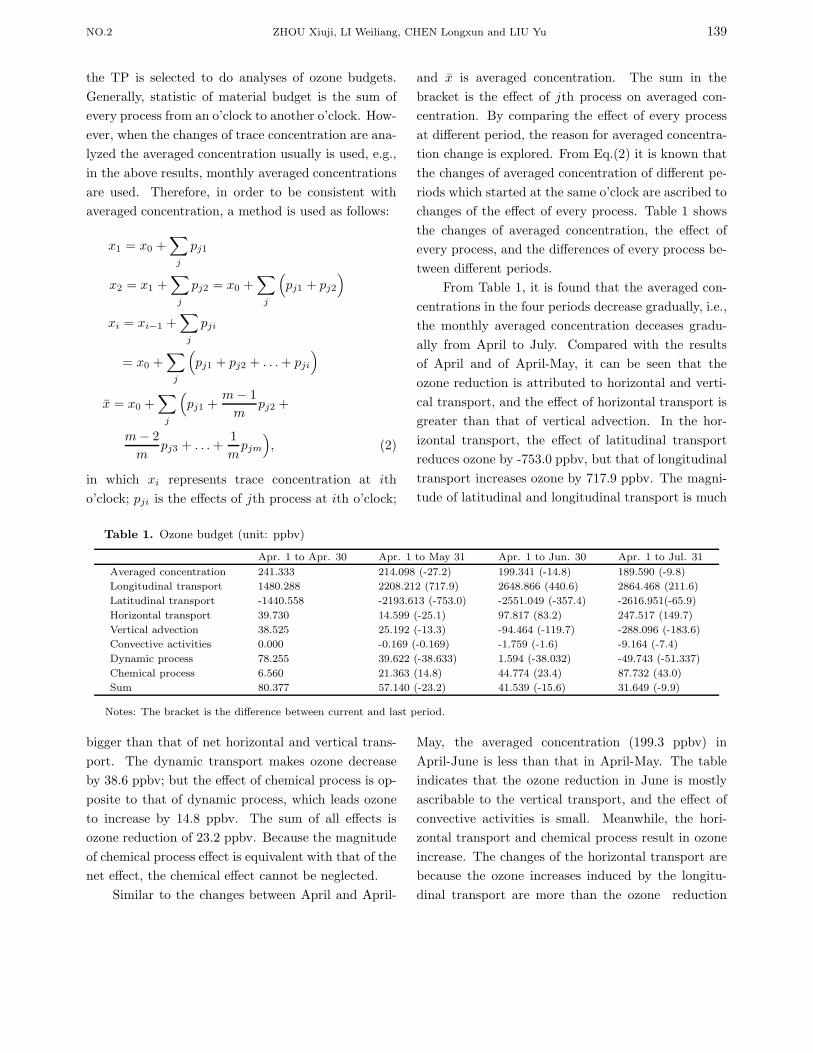
the TP is selected to do analyses of ozone budgets.

Generally, statistic of material budget is the sum of

every process from an o’clock to another o’clock. How-

ever, when the changes of trace concentration are ana-

lyzed the averaged concentration usually is used, e.g.,

in the above results, monthly averaged concentrations

are used. Therefore, in order to be consistent with

averaged concentration, a method is used as follows:

x1 = x0 +∑

j

pj1

x2 = x1 +∑

j

pj2 = x0 +∑

j

(

pj1 + pj2

)

xi = xi−1 +∑

j

pji

= x0 +∑

j

(

pj1 + pj2 + . . . + pji

)

x = x0 +∑

j

(

pj1 +m − 1

mpj2 +

m − 2

mpj3 + . . . +

1

mpjm

)

, (2)

in which xi represents trace concentration at ith

o’clock; pji is the effects of jth process at ith o’clock;

and x is averaged concentration. The sum in the

bracket is the effect of jth process on averaged con-

centration. By comparing the effect of every process

at different period, the reason for averaged concentra-

tion change is explored. From Eq.(2) it is known that

the changes of averaged concentration of different pe-

riods which started at the same o’clock are ascribed to

changes of the effect of every process. Table 1 shows

the changes of averaged concentration, the effect of

every process, and the differences of every process be-

tween different periods.

From Table 1, it is found that the averaged con-

centrations in the four periods decrease gradually, i.e.,

the monthly averaged concentration deceases gradu-

ally from April to July. Compared with the results

of April and of April-May, it can be seen that the

ozone reduction is attributed to horizontal and verti-

cal transport, and the effect of horizontal transport is

greater than that of vertical advection. In the hor-

izontal transport, the effect of latitudinal transport

reduces ozone by -753.0 ppbv, but that of longitudinal

transport increases ozone by 717.9 ppbv. The magni-

tude of latitudinal and longitudinal transport is much

Table 1. Ozone budget (unit: ppbv)

Apr. 1 to Apr. 30 Apr. 1 to May 31 Apr. 1 to Jun. 30 Apr. 1 to Jul. 31

Averaged concentration 241.333 214.098 (-27.2) 199.341 (-14.8) 189.590 (-9.8)

Longitudinal transport 1480.288 2208.212 (717.9) 2648.866 (440.6) 2864.468 (211.6)

Latitudinal transport -1440.558 -2193.613 (-753.0) -2551.049 (-357.4) -2616.951(-65.9)

Horizontal transport 39.730 14.599 (-25.1) 97.817 (83.2) 247.517 (149.7)

Vertical advection 38.525 25.192 (-13.3) -94.464 (-119.7) -288.096 (-183.6)

Convective activities 0.000 -0.169 (-0.169) -1.759 (-1.6) -9.164 (-7.4)

Dynamic process 78.255 39.622 (-38.633) 1.594 (-38.032) -49.743 (-51.337)

Chemical process 6.560 21.363 (14.8) 44.774 (23.4) 87.732 (43.0)

Sum 80.377 57.140 (-23.2) 41.539 (-15.6) 31.649 (-9.9)

Notes: The bracket is the difference between current and last period.

bigger than that of net horizontal and vertical trans-

port. The dynamic transport makes ozone decrease

by 38.6 ppbv; but the effect of chemical process is op-

posite to that of dynamic process, which leads ozone

to increase by 14.8 ppbv. The sum of all effects is

ozone reduction of 23.2 ppbv. Because the magnitude

of chemical process effect is equivalent with that of the

net effect, the chemical effect cannot be neglected.

Similar to the changes between April and April-

May, the averaged concentration (199.3 ppbv) in

April-June is less than that in April-May. The table

indicates that the ozone reduction in June is mostly

ascribable to the vertical transport, and the effect of

convective activities is small. Meanwhile, the hori-

zontal transport and chemical process result in ozone

increase. The changes of the horizontal transport are

because the ozone increases induced by the longitu-

dinal transport are more than the ozone reduction


resulted from the latitudinal transport. The net sum

of ozone changes is the ozone reduction of 15.6 ppbv.

Like the ozone changes in April-June, the effect of ev-

ery process on ozone becomes stronger in April-July

than that in June.

From the above analyses of April-May, April-

June, and April-July, it is found that in May, i.e., early

period of the TP ozone valley, the horizontal transport

is the main part of the dynamic process that results

in the TP ozone valley. However, in June and July

the vertical transport becomes main part of dynamic

process.

The effect of the gaseous chemical process brings

about ozone increases that are more than the net

changes sometimes, thus the chemical effect is also im-

portant.

5.3 Cause for formation of the TP ozone val-

ley in summer

From the above analyses, it can been seen that

when the ozone valley occurs and develops, the trans-

port process of ozone plays the main role, and the

chemical process partly compensates the ozone reduc-

tion by the transport process. In the dynamic trans-

port process of ozone, the horizontal transport process

plays a chief role of the ozone reduction in May. The

vertical transport process gradually plays a main role

of the ozone reduction in June and July. Effect of con-

vective activities rises little by little so that this effect

cannot be overlooked in July. Synthesized analyses

of model results and weather, we further depict the

dynamic and chemical process in the formation and

development of the TP ozone valley. In May, early

period of the TP ozone valley, the formation of the

TP ozone valley is primary because South Asian high

moves northwestward to bring ozone of lower concen-

tration from low latitudes. Then, while South Asian

high moves over the TP and its intensity strength-

ens, ozone of low concentration from low troposphere

around the TP is transported into the upper tropo-

sphere and lower stratosphere over the TP. Conse-

quently, the vertical transport plays a main role of the

TP ozone valley, but the horizontal transport com-

pensates partly the effect of the vertical advection. At

the same time, the effect of chemical process plays an

important role, and can not be overlooked.

6. The deepening of the TP ozone valley and

prediction of the TP TCO trend

Zhou et al. (1995) discovered that there is the TP

Fig.18. Seasonal variation of the difference between a site (31◦N, 90◦E) and its zonalaverage with height (unit:10−9 V V−1).


ozone valley in summer, and TCO decrease trend in

Lasha is quicker than that over East China of the same

latitude. Since Lasha is located in the area of TP

ozone valley, we wonder what is the trend of TCO over

the TP? Based on TOMS data from 1979 to 1992 (ver-

sion 7), Liu and Li (2001) calculated global TCO trend

and verified their reliability after the TOMS data is

handled by moving average.

Figure 19 depicts TCO trend over China, which

is based on TOMS data handled by moving average

to filter QBO, seasonal variation, etc., and inspects

with the 95% reliability, where the shadow area repre-

sents that the reliability is lower than 95%. From this

figure, it is found that the TCO decreases over most

of China except for Hainan Island, and their reliabil-

ity is more than 95%. TCO decrease trends increase

with latitude increasement. The maximum of the de-

crease trend appears in Northeast China, which is also

a large center of TCO decrease trend with more than

0.5% per year. Meanwhile, the figure shows that there

is a large center of TCO decrease trend over the TP

with more than 0.3% per year, but the TCO decrease

trend is about 0.2% per year over East China.

Because the site (32.5◦N, 88◦E) is a center of

TCO decrease trend in June, the sites (32.5◦N, 88◦E;

32.5◦N, 120◦E) are selected to represent the TP and

East China respectively. Table 2 exhibits TCO trends

at these sites, the trends of both TCO difference, and

their reliability, in which “×” represents that the reli-

ability is less than 95%, the other represent that the

Fig.19. Trend of total column ozone (unit: % yr−1) .

Fig.20. Area of deep ozone valley in June over the Ti-

betan Plateau. (Solid line is 280 DU of ozone, dashed

line represents ozone decrease rate, and shaded area

represents that it does not reach 95 % confidence.)

reliability is more than 95%. From the table, it is seen

that in January and June the reliability of the trend

of TCO and TCO difference between the two sites is

more than 95%. Because the TP ozone valley exists

in June and solar radiation is strong in this time, the

TP ozone valley in June is given more attention. From

Fig. 20, it is found that there is a large center of TCO

decrease trend over the TP in June, which is 0.3% per

year. And the TCO difference between the TP and

East China increase with more than 95% confidence.

Therefore, there is a deepening trend of TP ozone val-

ley. Figure 20 shows that the area of the deepening

trend is from 78◦ to 94◦E and from 29◦ to 33◦N (about

450 000 km2). Compared with TCO trend over other

area of the same latitude, the trend over the TP is one

of strong centers of TCO decrease trend.

The TP covers a quarter of the whole China. Be-

cause there is TP ozone valley in summer and it deep-

ens, it will lead to solar UV radiation increases, and

influence Tibetan human beings, ecosystem, and envi-

ronment strongly. Therefore, future TCO trend over

the TP is given close attention. Liu et al. (2001)

explored TCO trend over the TP with a 2-D global

chemical model.

Figure 21 shows the pattern of TCO change over

the TP: TCO decreases from 1980 to 1993; it reaches

low extremum in 1993; it recovers rapidly from 1993


Table 2. Trend of TCO at (32.5◦N, 88◦E) and (32.5◦N, 120◦E) and their difference

Jan. Feb. March April May June July Aug. Sep. Oct. Nov. Dec.

88◦E -0.58 -0.26 -0.57 -0.37 -0.36 -0.34 -0.16 -0.08 -0.10 -0.19 -0.36 -0.11

REL × × × × × ×

120◦E -0.38 -0.29 -0.26 -0.10 -0.37 -0.19 -0.00 0.02 -0.02 -0.06 -0.32 -0.16

REL × × × × × × ×

DIF 3.75 -0.92 4.21 2.35 -0.45 0.917 1.38 0.947 0.812 1.85 0.655 -1.00

REL × × × × × × × ×

Notes: REL represents reliability; DIF represents difference; and “×” represents the confidence lower than 95%.

Fig.21. Trend of modeled total column ozone over the

Tibetan Plateau.

to 1995; then it recovers gradually, but until 2050 it

does not reach that of 1980. Under the condition of

TP special circulation, TCO recovers faster than under

zonal mean condition. It illustrates that the TP spe-

cial circulation is not the main reason that the strong

center of TCO decrease trend forms over the TP.

7. Summary

This paper reviewed the main results in the last

decade with respect to the discovery of low center

of TCO over the TP in summer, and its formation

mechanism. Some important advances are summa-

rized as follows: The fact is discovered that there is

the TP ozone valley in summer, and the features of

the background circulation over the TP are analyzed;

it is confirmed that the TP is a pathway of mass ex-

change between troposphere and stratosphere, and it

influences the TP ozone valley; models reproduce the

TP ozone valley, and the formation mechanism are

explored; in addition, the analyses and diagnoses of

the observation data indicated that not only there is

the TP ozone valley, but also TCO decrease trend

over the TP is one of strong centers of TCO decrease

trend in the same latitude; finally, the model predicts

future TCO change over the TP.

Because under the condition of TP special circu-

lation ozone change over the TP results from net role

of dynamical, physical, and chemical processes which

involve many natural and anthropogenic effects, it

is difficult to understand them definitely now, such

as the TCO decrease trend over the TP, dynamical

and thermo-dynamical role cannot explain this phe-

nomenon, this should be ascribed to other reasons.

Maybe, heterogeneous reaction and clouds over the

TP are related to that, which is a nonlinear result of

dynamical, physical, and chemical processes. Because

the TP is a special and important region that could

influence climate and environment of East Asia and

globe, we hope to have opportunities to further ex-

plore the above issues.

REFERENCES

Bojkov, R., 1994: The ozone layer-recent development.

Bulletin of WMO, 43, 113-116.

Bian Jianchun, Li Weiliang, and Zhou Xiuji, 1997: Anal-

ysis of the seasonal variation feature of the wind

structure over Tibetan Plateau and its surround-

ings. Ozone changes over China and its influences

on climate and environment. Zhou Xiuji ed. Chi-

nese Meteorological Press, Beijing. 257-273. (in

Chinese)

Cong Chunhua, Li Weiliang, and Zhou Xiuji, 2001: Mass

exchange between stratosphere and troposphere over

the Tibetan Plateau and its surroundings. Chinese

Science Bulletin, 47, 508-512. (in Chinese)

Fu Chao, Li Weiliang, and Zhou Xiuji, 1997: Numerical

simulation of the formation of “ozone valley over

Tibetan Plateau” in summer. Ozone changes over

China and its influences on climate and environ-

ment. Zhou Xiuji ed. Chinese Meteorological Press,


Beijing. 274-285. (in Chinese)

Li Weiliang and Yu Shengmin, 2001: Spatio-temporal

characteristics of aerosol distribution over Tibetan

Plateau and numerical simulation of radiative forc-

ing and climate response. Science in China, 44

(Supp), 375-384. (in Chinese)

Liu Yu and Li Weiliang, 2001: Deepening of ozone valley

over Tibetan Plateau and its possible effects. Acta

Meteor. Sinica, 59, 97-105. (in Chinese)

Liu Yu, Li Weiliang, and Zhou Xiuji, 2001: Prediction

of the trend of total column ozone over the Tibetan

Plateau. Science in China, 44 (Supp), 385-389. (in

Chinese)

Liu Yu, Li Weiliang, Zhou Xiuji, et al., 2003: Mechanism

of formation of the ozone valley over the Tibetan

Plateau in summer: Transport and chemical process

of ozone. Advance in Atmospheric Science, 20, 103-

109.

Muller, J., 1992: Geographical distribution and seasonal

variation of surface emission and deposition veloci-

ties of atmosphere in trace gases. J. Geophys. Res.,

97, 3787-3804.

Reiter and Gao Dongyi, 1982: Heating of the Tibet

Plateau and movements of the South High in spring.

Mon. Wea. Rev., 110, 1694-1711.

Ren Chuansen, Li Weiliang, Zhou Xiuji, et al., 1997:

Numerical simulation of ozone distribution and its

variation mechanism. Acta Meteor. Sinica, 11, 129-

142.

Sundet, J. K., 1997: Model studies with a 3-D Global

CTM using ECWMF data. Ph.D dissertation. Dept.

of Geophysics, University of Oslo, Norway.

Wei Dingwen, Zhao Yanliang, and Qin Fang, 1994: Ab-

normal change of ozone layer at Beijing and Kun-

ming. Chinese Science Bulletin, 39 (16), 1509-1511.

(in Chinese)

Wei M. Y., 1987: A new formulation of the exchange of

mass and trace constituents between stratosphere

and troposphere. J. Atmos. Sci., 44, 3079-3085.

Wang Wei-Chying and Ryan P. B., 1983: Overlaping ef-

fects of atmospheric H2O, CO2 and O3 on the CO2

radiative effect. Tellus, 35B, 81-91.

Wild, O., X. Zhu, M. J. Prather, et al., 2000: Accurate

simulation of in and below cloud photolysis in tro-

posphere chemical model. J. Atmos. Chem., 37,

245-282.

Yanai, M., Li Chengfeng, and Song Zhangshan, 1991:

Seasonal heating of the Tibetan Plateau and its ef-

fects on the evolution of the Asian summer monsoon.

J. Meteor. Soc. Jap., 70, 319-351.

Zhou Xiuji, Luo Chao, and Li Weiliang, 1995: Total

column ozone over China and center of low total

column ozone over the Tibetan Plateau. Chinese

Science Bulletin. 40 (15), 1396-1398. (in Chinese)

Zou Han, 1996: Seasonal variation and trends of TOMS

ozone over Tibet. Geophys. Res. Let., 23, 1029-

1032.

Zou Han, Gao Yongqi, and Zhou Libo, 1998: Low to-

tal column ozone over large mountains and heating

fields. Research on Climate and Environment, 3,

209-217. (in Chinese)

study on ozone change over the tibetan plateau2 zhou xiuji, li weiliang, chen longxun and liu yu 129...

Documents