Ultrasonics 51 (2011) 1014–1025

Contents lists available at ScienceDirect

Ultrasonics

journal homepage: www.elsevier .com/ locate/ul t ras

Study on the bubble transport mechanism in an acoustic standing wave field

Xiaoyu Xi a, Frederic B. Cegla a,⇑, Michael Lowe a, Andrea Thiemann b, Till Nowak b, Robert Mettin b,Frank Holsteyns c, Alexander Lippert c

a Department of Mechanical Engineering, Imperial College London, London SW7 2AZ, UKb Christian Doppler Laboratory for Cavitation and Micro-Erosion, Drittes Physikalisches Institut, Georg-August-Universität Göttingen, Friedrich-Hund-Platz 1,37077 Göttingen, Germanyc Lam Research AG, SEZ-Strasse 1, 9050 Villach, Austria

a r t i c l e i n f o

Article history:Received 28 February 2011Received in revised form 19 May 2011Accepted 31 May 2011Available online 13 June 2011

Keywords:BubblesUltrasonic bubble manipulationBjerkness forceUltrasonic transducers1D Network model

0041-624X/$ - see front matter � 2011 Elsevier B.V.doi:10.1016/j.ultras.2011.05.018

⇑ Corresponding author.E-mail address: f.cegla@imperial.ac.uk (F.B. Cegla)

a b s t r a c t

The use of bubbles in applications such as surface chemistry, drug delivery, and ultrasonic cleaning etc.has been enormously popular in the past two decades. It has been recognized that acoustically-drivenbubbles can be used to disturb the flow field near a boundary in order to accelerate physical or chemicalreactions on the surface. The interactions between bubbles and a surface have been studied experimen-tally and analytically. However, most of the investigations focused on violently oscillating bubbles (alsoknown as cavitation bubble), less attention has been given to understand the interactions between mod-erately oscillating bubbles and a boundary. Moreover, cavitation bubbles were normally generated in situby a high intensity laser beam, little experimental work has been carried out to study the translationaltrajectory of a moderately oscillating bubble in an acoustic field and subsequent interactions with thesurface. This paper describes the design of an ultrasonic test cell and explores the mechanism of bubblemanipulation within the test cell. The test cell consists of a transducer, a liquid medium and a glass back-ing plate. The acoustic field within the multi-layered stack was designed in such a way that it was effec-tively one dimensional. This was then successfully simulated by a one dimensional network model. Themodel can accurately predict the impedance of the test cell as well as the mode shape (distribution ofparticle velocity and stress/pressure field) within the whole assembly. The mode shape of the stackwas designed so that bubbles can be pushed from their injection point onto a backing glass plate. Bubbleradial oscillation was simulated by a modified Keller–Miksis equation and bubble translational motionwas derived from an equation obtained by applying Newton’s second law to a bubble in a liquid medium.Results indicated that the bubble trajectory depends on the acoustic pressure amplitude and initial bub-ble size: an increase of pressure amplitude or a decrease of bubble size forces bubbles larger than theirresonant size to arrive at the target plate at lower heights, while the trajectories of smaller bubbles areless influenced by these factors. The test cell is also suitable for testing the effects of drag force on thebubble motion and for studying the bubble behavior near a surface.

� 2011 Elsevier B.V. All rights reserved.

1. Introduction

The understanding of interactions between a boundary and airbubbles in aqueous solutions is of particularly industrial interestsince ultrasound-driven bubbles have substantial physical andchemical effects on the target surface [1]. It is well-known thatthe forces generated from cavitation bubbles are sufficient to erodemetal surfaces [2], clean contaminated wafers [3–5], and inducecell lysis or cell membrane porosity [6–13]. Numerous investiga-tions on the mechanism of bubble oscillation near a boundary havebeen carried out for decades, e.g. [14,15]. A comprehensive reviewof this topic can be found in recent work by Lauterborn and Kurz

All rights reserved.

.

[16]. Despite the successful studies of cavitation bubble inducedphysical and chemical effects, less attention has been given tounderstand the mechanism of interactions between moderatelyoscillating bubbles and a surface. Moreover, most of the previousstudies focused on the collapse and consequent shape distortionof laser-generated bubbles which have already been placed nextto a target area. However, the means to effectively move moder-ately oscillating bubbles to the appointed target in the first placeis still open to question. Multiple bubble transport is also prefera-ble in real life applications, but to date there are only few reportson the experimental configuration for this purpose.

To achieve bubble motion control, acoustic systems are typi-cally fabricated based on a layered resonator. The main part ofthe resonator is a piezoelectric material which is bonded to severalmatching layers. Acoustical standing waves can be generated in a

X. Xi et al. / Ultrasonics 51 (2011) 1014–1025 1015

liquid layer (matching layer) which is terminated by a reflector. Aone-dimensional equivalent network model (1D model) has beenwidely used for predicting the acoustic responses of such multi-layered structures [17,18]. In the 1D model, characteristics of asound field including pressure profile and amplitude are calculatedbased on the properties of the matching layers. At a certain fre-quency, the mode shape (particle velocity or stress/pressure distri-bution) of an acoustic field can then be determined. Similarresonator devices have been used by many authors to study parti-cle manipulation [19–22] and cell localization [23–26].

Few researchers, however, have applied the resonator systemto investigate bubble motion and control. This is believed to bedue to the fact that bubble motion in an acoustic field not onlydepends on the characteristics of the sound field, but also onthe bubble oscillation which complicates the analysis of the bub-ble movement. A gas bubble driven below its resonance fre-quency in a weak standing wave field moves towards thepressure anti-node, while a bubble driven above its resonance fre-quency moves towards the pressure node instead. This effect isattributed to the primary Bjerknes force on a bubble and has beenstudied extensively by King [27], Yoshioka et al. [28], Eller [29],Crum [30], Lee and Wang [31] and Doinikov [32]. On the otherhand, in a high intensity acoustic field, two types of bubble trans-lational instabilities have been recognized. The first one, alsoknown as ’dancing’ motion, refers to the bubble erratic behaviorswhen bubbles travel in a sound field. It was first observed byGaines [33], Strasberg and Benjamin [34] and Eller and Crum[35] and later on investigated by Mei and Zhou [36], Feng andLeal [37] and Doinikov [38] in more detail. A generally acceptedexplanation for this phenomenon attributes the bubble surfacemodes, which come into existence once the acoustic pressureamplitude exceeds a threshold value, as the main cause. The sec-ond type of translational instability results from the fact that theprimary Bjerknes force acting on a bubble changes sign at higheracoustic pressure [39,40]. This change is a result of the increasedphase shift between bubble volumetric pulsation and the drivingpressure. This behavior was reported by Miller [41], Khanna et al.[42], and Kuznetsova et al. [43]. Theoretical investigations werecarried out by Abe et al. [44], Watanabe and Kukita [45] and morerecently were extended by Doinikov [46] and Mettin and Doini-kov [47]. However, there remains a need for an experimentalmethod to be developed to effectively move bubbles to a bound-ary and excite bubbles near the boundary surface.

The purpose of this study is to describe a bubble transport tech-nique which uses a multi-layered resonator to push bubbles to areflector surface and examine the bubble behavior when theymigrate in the sound field as well as close to the target surface.In Section 2, details of the experimental setup which were usedto study the translational and oscillatory motion of bubbles aredescribed. Section 3 provides the theoretical models of bubblemotion in an acoustic standing wave field. Comparisons betweenthe theoretical predictions and experimentally obtained resultsare given in Section 4. A conclusion is provided in Section 5.

2. Theory and experimental setup

As described in the introduction, the means to effectively movebubbles to a region of interest is critical in developing the bubblecontrol technique using acoustic wave. Three tools for the studyof bubble transport mechanism and bubble oscillatory motionare presented here. Firstly, a bubble generator which is based onthe principle of electrolysis is used. Secondly, a standing wave fieldis generated by a multi-layered structure and the characteristics ofthis field are simulated by a 1D model. The 1D model allows us toaccurately predict the acoustic responses of the device including

impedance and pressure amplitude in the layered structure.Thirdly, details of bubble translational and oscillatory motion arerecorded by an optical observation system. Using these three tools,we determined the bubble trajectories within the test cell andstudied the bubble oscillation near a surface.

2.1. Bubble generator

Bubbles used in this study are generated by an electrolysismethod. Two wires (tin-coated copper) are connected to a DCpower supply (TNG 35, Voltcraft, Germany) and the electrical po-tential is set to 5 V. The free ends of the wires are placed atx = 3 mm (the origin of the coordinate system is set at the centerof the transducer-water boundary as shown in Fig. 2). Hydrogengas bubbles are generated at the tip of the negative electric wireand escape from there afterwards. The bubble diameter varies from10 lm when there is no ultrasound, up to 200 lm when the ultra-sound device is switched on. The large bubbles are the outcomes ofbubble coalescence processes which are significantly enhanced inthe presence of ultrasound.

2.2. 1D model for acoustic standing wave field

The method implemented in our 1D model is the modifiedequivalent electrical network of a transducer. In the model, atransducer is treated as a purely electrical circuit and can be ana-lyzed by conventional circuit analysis techniques. The 1D modelhas been verified to accurately predict acoustic responses of mul-ti-layered structures within the first few resonance frequencies.The model was described in detail by Wilcox et al. [17] and herea short outline is presented. The basic idea of this approach isshown in Fig. 1. The piezoelectric layer is represented as athree-port electrical network which is described by the followingmatrix equation.

F1

F2

V3

0B@

1CA ¼ �i

AZpiezocotkpiezodpiezo AZpiezocsckpiezodpiezo hx1=xAZpiezocsckpiezodpiezo AZpiezocotkpiezodpiezo hx1=x

hx1=x hx1=x 1=xC0

0B@

1CA

v1

v2

I3

0B@

1CAð1Þ

where Fi and vi (i is the index) are the force and particle velocity atthe two acoustic ports. V3 and I3 are the voltage and current appliedto the electric port of the piezoelectric material. A, Zpiezo, dpiezo, andkpiezo are the area, characteristic impedance, thickness, and acousticwave number of the piezoelectric layer respectively. hx1 is the trans-mitting constant of the piezoelectric material in the x direction(longitudinal direction). C0 is the clamped (zero strain) capacitance.x is the angular frequency.

For a non-piezoelectric layer, the input force and velocity (F1

and v1) are related to the output force and velocity (F2 and v2) bya matrix

F2

v2

� �¼

coskLdL �iAZLsinkLdL

�ði=AZLÞsinkLdL coskLdL

� �F1

v1

� �¼ TL

F1

v1

� �ð2Þ

where ZL, dL, and kL are the characteristic impedance, thickness, andacoustic wave number of the layer respectively. A is the area of thelayer which is the same as the piezoelectric one, TL is the transfermatrix of this non-piezoelectric layer.

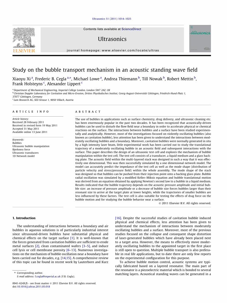
As the acoustic generator in Fig. 1a is represented by a numberof cascaded two-port (non-piezoelectric layer) networks and athree-port (piezoelectric layer) one, it is possible to calculate theacoustic response of the whole stack by reducing the continuousnetworks to a single two-port one. The 3 by 3 matrix in Eq. (1) isreplaced by an equivalent symmetrical one for the sake of simplic-ity and the notations in Wilcox’s work are used here [17].

(a)

(b)

Fig. 1. (a) A diagram of a physical acoustic standing wave generator. (b) The piezoelectric layer is represented by a three-port network.

1016 X. Xi et al. / Ultrasonics 51 (2011) 1014–1025

F1

F2

V3

0B@

1CA ¼

Z11 Z12 Z13

Z21 Z22 Z23

Z31 Z32 Z33

0B@

1CA

v1

v2

I3

0B@

1CA ð3Þ

The ratios �F1/v1 and �F2/v2 are represented by Z0B and Z0A respec-tively, and Eq. (3) can be reduced to a 2 by 2 matrix ZPZ using Z0B

F2

V3

� �¼

Z22 � Z12Z21Z0BþZ11

Z23 � Z21Z13Z0BþZ11

Z32 � Z12Z31Z0BþZ11

Z33 � Z13Z31Z0BþZ11

0@

1A v2

I3

� �

¼Z022 Z023

Z032 Z033

!v2

I3

� �¼ Zpz

v2

I3

� �ð4Þ

Then using Z0A, the electrical input impedance of the transducerZIN = V3/I3 can be found by

ZIN ¼ Z033 �Z0223

Z0A þ Z022

ð5Þ

The input electrical quantities (V3, I3) can be related to the outputquantities (F2, v2) by a transfer matrix TPZ, which is derived by rear-ranging Eq. (4).

F2

v2

� �¼

Z022Z032

Z023 �Z022Z033

Z032

1Z032

� Z033Z032

0@

1A V3

I3

� �¼ Tpz

V3

I3

� �ð6Þ

Also, the transfer matrices for the matching layers are representedby TLn(n = 1,2, . . .) which are similar to the TL in Eq. (2). n is the layer

index. To calculate the transfer matrix (T) which represents thesystem, the transfer matrix TPZ is pre-multiplied by the TLn andthe system transfer matrix T is found

T ¼ TLn . . . TL2TL1TPZ ð7Þ

For a transducer, T relates the voltage/current (V3 and I3) of the in-put signal to the force/velocity (Fout and vout) in the output mediumthrough Eq. (8).

Fout

vout

� �¼ T

V3

I3

� �ð8Þ

2.3. Acoustical standing wave generator

The multi-layered resonator has been widely used in manyapplications such as particle manipulation, cell separation, andultrasonic transducer design. An acoustical standing wave field isgenerally established along the structure (axial direction). Thesound field is believed to be uniformly distributed in the radialdirection (or directions normal to the axial axis for non-cylindricalshape structure) and this assumption is only valid when the lengthof the structure is larger than its width and the width is less thanhalf of the standing wave wavelength (the use of isotropic materi-als is assumed). As the sound field within the multi-layered struc-ture only varies in the axial direction, the 1D model can accuratelypredict the acoustic responses of such resonators. To clearly illus-trate the bubble transport mechanism, it is favorable to design a

X. Xi et al. / Ultrasonics 51 (2011) 1014–1025 1017

simple standing wave field with one pressure node and one pres-sure anti-node along the axial direction in a liquid medium(matching layer) and with little variations in the radial direction.Within this acoustic field, the bubble migrating direction can beeasily categorized either towards the pressure node or pressureanti-node based on bubble size and acoustic pressure amplitude.It is well known that a resonant air bubble in water has a radiusof 30 lm at 100 kHz. The bubble generator produces bubbles ofabout 100 lm (radius) indicating resonance frequencies of about30 kHz. Therefore, in order to ensure operation above the reso-nance frequencies of the bubbles a stack with the second reso-nance frequency of 108 kHz was designed.

A schematic diagram of the setup is shown in Fig. 2. A continuoussinusoidal wave is transmitted from a waveform generator (AFG3021, Tektronix, USA) to a transducer via an amplifier (HSA 4101,NF corporation, Japan). The input signal is monitored by an oscillo-scope (TDS 220, Tektronix, USA). A standing wave is established inthe stack along the x axis and has negligible variations in the y andz directions (see Section 4.1). The origin of the coordinates is set atthe center of the transducer-water boundary (x = 0, y = 0, z = 0). Awater layer constrained within a brass chamber is placed betweenthe transducer and a glass plate (from x = 0 mm to x = 5 mm). Toallow light to pass through the water layer for optical observations,two glass windows are fit on the sides of the brass chamber. Bubblesescape from the wire connected to the negative port of the DC powersupply and migrate in the water medium. The wires connected to theDC power supply were positioned at x = 3 mm.

The acoustic standing wave generator consisted of a roundtransducer, a square liquid (deionized water) layer of 5 mm thick-ness held in a brass block (5 mm by 5 mm by 5 mm) and a roundborosilicate glass plate of 0.1 mm thickness (VWR, UK). To fit thetwo glass windows on the water sides for the following opticalobservations, the cross section of the liquid layer was chosen as asquare shape (5 mm by 5 mm). The transducer was fabricatedout of a lead zirconate titanate (PZT) disk (PCM 51, EP ElectronicComponents Ltd, UK), a backing brass bar, a front brass bar withthickness of 2 mm, 3 mm and 9 mm respectively. The diameter ofthe transducer is 5 mm.

To examine the validity of the 1D model, the pressure field inthe water layer at 108 kHz was measured by a calibrated needle

Fig. 2. A schematic diagram of the ac

hydrophone (HPM1/1, Precision Acoustics, UK) and compared withthe result obtained from the 1D model. A diagram of the testingsetup is shown in Fig. 3. The hydrophone is fixed on a three dimen-sion scanning frame (3 axis motorized scanning system, Time andPrecision Industries Ltd, UK) which is controlled by a computer.The hydrophone is powered by a DC power supply (DC3, PrecisionAcoustics, UK) and is used to measure the pressure profile in the x,y and z directions in the water layer. The pressure amplitudesalong the x axis are measured from point A (see Fig. 3) at the centerof the base of the water column to point B (see Fig. 3), which is atthe center of the top of the water column with a step size of0.5 mm. The difference between the test cells shown in Fig. 3 and2 is that the glass plate which is used as a reflector in Fig. 2 is re-moved in the hydrophone measurement case. It needs to bepointed out that the purpose of the hydrophone measurement isto solely examine the 1D model predictions so that confidence inits validity can be obtained. As the 1D model treats each matchinglayer in the same way, it is reasonable to accept that the pressureprofile of a testing cell with the thin glass plate (sound soft bound-ary) can be accurately predicted by the 1D model which is verifiedin the case without the additional glass plate.

2.4. Optical observation system

A high speed camera (FastCam SA5, Photron, USA) was used toinvestigate the bubble moving trajectory and oscillatory motion.The maximum frame rate of the camera is 1 Mega frames/s andis therefore suitable for analyzing bubble motion in pressure fieldsoscillating at hundreds of kilo-Hertz. Fig. 4 shows the schematicdiagram of the measurement setup. A backing light source waspositioned opposite to the high speed camera with the standingwave generator in the middle. A viewing window of 3.9 mm by3.8 mm was chosen to cover the glass plate and the bubble injec-tion point at the same time. Recorded videos were transmittedback to a computer and were analyzed by an object tracking pro-gram written in Matlab (Mathworks Inc., USA). In the Matlab pro-gram, the center of a bubble was tracked in each frame and a plotof the bubble center positions with respect to time was obtained.The dimensions of objects in a video were calibrated with a stan-dard 300 lm long stick.

oustic standing wave generator.

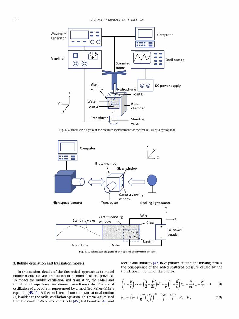
Fig. 3. A schematic diagram of the pressure measurement for the test cell using a hydrophone.

Fig. 4. A schematic diagram of the optical observation system.

1018 X. Xi et al. / Ultrasonics 51 (2011) 1014–1025

3. Bubble oscillation and translation models

In this section, details of the theoretical approaches to modelbubble oscillation and translation in a sound field are provided.To model the bubble oscillation and translation, the radial andtranslational equations are derived simultaneously. The radialoscillation of a bubble is represented by a modified Keller–Miksisequation [48,49]. A feedback term from the translational motionð _xÞ is added to the radial oscillation equation. This term was missedfrom the work of Watanabe and Kukita [45], but Doinikov [46] and

Mettin and Doinikov [47] have pointed out that the missing term isthe consequence of the added scattered pressure caused by thetranslational motion of the bubble.

1�_Rc

!R€Rþ 3

2�

_R2c

!_R2 � 1

q1þ

_Rc

!Psc �

Rqc

_Psc �_x2

4¼ 0 ð9Þ

Psc ¼ P0 þ2rR0

� �R0

R

� �3c

� 2rR� 4g _R

R� P0 � Pex ð10Þ

Fig. 5. Calculated impedance of test cell without (solid line) and with (dotted line)the glass plate. The frequencies used in the calculation are from 50 kHz to 300 kHz.

Fig. 6. Measured (scatter line) and simulated (solid line) pressure profiles in thewater layer at 108 kHz. The pressure distribution is measured from the center of thebase of the water column (A) to the center of the top of the water column (B) asshown in Fig. 3. The input signal amplitude is 1.8 V. The solid vertical line on the leftside indicates the position (x = 1.7 mm) where the y and z directions measurementshown in Fig. 7 was carried out. The dashed vertical line on the right side shows theposition of the bubble injection point (x = 3 mm).

(a)

(b)

Fig. 7. Pressure profiles measured by the hydrophone in the y axis and z axis at108 kHz for input signal of 1.8 V and x = 1.7 mm. (a) measured pressure profile inthe y axis; (b) measured pressure profile in the z axis.

Fig. 8. A simulated pressure distribution of the multi-layered structure (with theglass layer) at 108 kHz for input signal of 2 V.

X. Xi et al. / Ultrasonics 51 (2011) 1014–1025 1019

where R is the time-varying radius of a bubble, R0 is the equilibriumradius. c and q are the sound velocity and density of the liquidrespectively. P0 is the hydrostatic pressure, r is the surface tension,c is the polytropic exponent of the gas within the bubble, g is theviscosity of the liquid. _x is the translational velocity of the bubblein the x axis. Pex is the external driving signal which is defined asa standing wave here:

Pex ¼ PasinðxtÞsinðkdÞ ð11Þ

where Pa is the pressure amplitude, x is the angular frequency, andk is the wave number. As only a one dimensional standing wave isconsidered here, d is the distance between the center of the bubbleand a pressure anti-node along the x axis as shown in Fig. 2.

The translational motion of a bubble is derived based on New-ton’s second law, given by

€xþ 3 _R _xR¼ 3Fex

2pqR3 ð12Þ

€yþ 3 _R _yR¼ 3Fey

2pqR3 ð13Þ

where x and y are the positions of the bubble center on the x and yaxes as shown in Fig. 2. The overdot denotes the time derivative. Ina two dimensional plane, the coordinates of the bubble center aregiven by the time-varying variables x and y. Fex and Fey are the exter-nal force in the x axis and y axis directions respectively. In the x axisdirection, the Fex is equal to the sum of the primary Bjerknes force(Fp) and the viscous drag force (Fvx) [50]

Fig. 9. The relationship between bubble resonance frequency and bubble radius.Bubble radius ranges from 10 lm to 300 lm.

1020 X. Xi et al. / Ultrasonics 51 (2011) 1014–1025

Fp ¼ �4p3

R3kPasinðxtÞcosðkdÞ ð14Þ

Fvx ¼ �12pgRð _x� veÞ ð15Þ

where ve is the liquid velocity that is generated by the imposedacoustic field at the center of the bubble

ve ¼Pa

qccosðxtÞcosðkdÞ ð16Þ

In the y axis direction, the Fey is the sum of buoyancy force (Fb) andviscous force (Fvy) [50]

Fb ¼4p3

R3ðq� qgasÞ ð17Þ

Fvy ¼ �12pgR _y ð18Þ

where qgas is the density of gas inside a bubble.As described in Section 2.3, the direction of the bubble trajec-

tory also depends on the bubble resonance frequency which is gi-ven by [50]

fres ¼1

2pR0

ffiffiffiffiffiffiffiffiffiffiffiffiffiffiffiffiffiffiffiffiffiffiffiffiffiffiffiffiffiffiffiffiffiffiffiffiffiffiffiffiffiffiffiffiffiffiffiffiffiffiffi3cP0

q1þ 2r

P0R0

� �� 2r

R0q

sð19Þ

If the acoustic standing wave field is weak and oscillating at a fre-quency above the bubble resonant frequency, bubbles are pushedto the pressure node, otherwise they travel to the pressure anti-node.

4. Results and discussion

In this section, the experimental results of bubble behavior inan acoustic standing wave field are presented and are comparedwith results predicted by the theoretical models. Firstly, a pressure

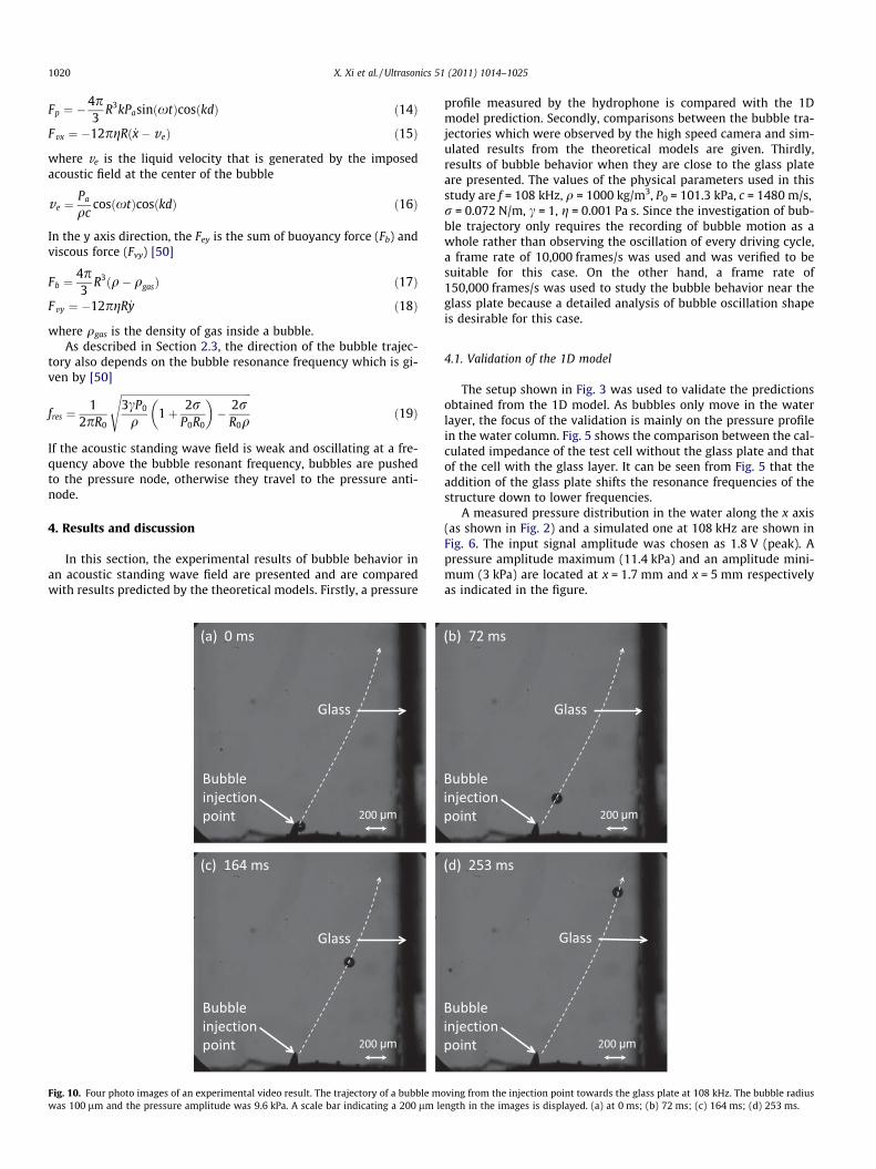
Fig. 10. Four photo images of an experimental video result. The trajectory of a bubble mwas 100 lm and the pressure amplitude was 9.6 kPa. A scale bar indicating a 200 lm le

profile measured by the hydrophone is compared with the 1Dmodel prediction. Secondly, comparisons between the bubble tra-jectories which were observed by the high speed camera and sim-ulated results from the theoretical models are given. Thirdly,results of bubble behavior when they are close to the glass plateare presented. The values of the physical parameters used in thisstudy are f = 108 kHz, q = 1000 kg/m3, P0 = 101.3 kPa, c = 1480 m/s,r = 0.072 N/m, c = 1, g = 0.001 Pa s. Since the investigation of bub-ble trajectory only requires the recording of bubble motion as awhole rather than observing the oscillation of every driving cycle,a frame rate of 10,000 frames/s was used and was verified to besuitable for this case. On the other hand, a frame rate of150,000 frames/s was used to study the bubble behavior near theglass plate because a detailed analysis of bubble oscillation shapeis desirable for this case.

4.1. Validation of the 1D model

The setup shown in Fig. 3 was used to validate the predictionsobtained from the 1D model. As bubbles only move in the waterlayer, the focus of the validation is mainly on the pressure profilein the water column. Fig. 5 shows the comparison between the cal-culated impedance of the test cell without the glass plate and thatof the cell with the glass layer. It can be seen from Fig. 5 that theaddition of the glass plate shifts the resonance frequencies of thestructure down to lower frequencies.

A measured pressure distribution in the water along the x axis(as shown in Fig. 2) and a simulated one at 108 kHz are shown inFig. 6. The input signal amplitude was chosen as 1.8 V (peak). Apressure amplitude maximum (11.4 kPa) and an amplitude mini-mum (3 kPa) are located at x = 1.7 mm and x = 5 mm respectivelyas indicated in the figure.

oving from the injection point towards the glass plate at 108 kHz. The bubble radiusngth in the images is displayed. (a) at 0 ms; (b) 72 ms; (c) 164 ms; (d) 253 ms.

Fig. 11. Bubble trajectories at different pressure amplitudes and the influences of pressure amplitude and bubble size on the bubble trajectory. (a1) for a large bubble (bubbleradius = 100 lm), the pressure amplitudes applied are 11.52 kPa (- - -), 9.6 kPa (—), 8.64 kPa (– –), 7.68 kPa (– � –), and 9.6 kPa for the experimental result (j); (a2) at 9.6 kPa,bubble radii are 130 lm (– � � –), 100 lm (—), 70 lm (� � �), and 100 lm for the experimental result (j); (b1) for a large bubble (bubble radius = 167 lm), the pressureamplitudes applied are 23.04 kPa (- - -), 19.2 kPa (—), 17.28 kPa (– –), 15.36 kPa (– � –), and 19.2 kPa for the experimental result (j); (b2) at 19.2 kPa, bubble radii are 200 lm(– � � –), 167 lm (—), 140 lm (� � �), and 167 lm for the experimental result (j); (c1) for a large bubble (bubble radius = 217 lm), the pressure amplitudes applied are 34.56 kPa(- - -), 28.8 kPa (—), 25.92 kPa (– –), 23.04 kPa (– � –), and 28.8 kPa for the experimental result (j); (c2) at 28.8 kPa, bubble radii are 280 lm (– � � –), 217 lm (—), 160 lm (� � �),and 217 lm for the experimental result (j). Driving frequency = 108 kHz.

X. Xi et al. / Ultrasonics 51 (2011) 1014–1025 1021

Only a small difference between the 1D model prediction and themeasured result is seen in Fig. 6. Uniform pressure distributionsalong the y axis and z axis are assumed here. This assumption is val-idated by the measurement of pressure field in the y and z directionsin the water layer (Fig. 7). The pressure profiles were measured in they axis and z axis directions at x = 1.7 mm. It can be seen from Fig. 7that slight variations existed in the y and z directions. These varia-tions, however, were small (within ±10%) so that the one-dimensionassumption used in our models is considered still to be valid.

Having established the 1D model’s validity by the experimentalmeasurements, it was used to predict the pressure distribution inthe x axis direction of a multi-layered structure with an additionalglass plate at the end. A typical result calculated from Eqs. (1)–(8)at 108 kHz is shown in Fig. 8. The input signal amplitude is 2 V(peak). A minimum pressure amplitude (1.2 kPa) and a maximumpressure amplitude (11.4 kPa) in the water layer are seen at thex = 5 mm and x = 2 mm respectively. Based on the previous discus-sion, bubbles are anticipated to migrate from the initial injectionpoint (x = 3 mm) to the glass plate (x = 5 mm) if the bubble sizesare larger than their resonance sizes. On the other hand, smallerbubbles move towards the pressure anti-node (x = 2 mm) instead.Based on Eq. (19), the bubble resonance frequency as a functionof bubble radius is displayed in Fig. 9. At 108 kHz, the bubble res-onance radius is 30 lm. The theory predicts that bubbles of radiilarger than 30 lm should move towards the pressure node locatedat x = 5 mm and bubbles smaller than this resonance size shouldmove towards the pressure anti-node at x = 2 mm.

4.2. Bubble trajectory in the water layer

The trajectory of a bubble moving from the injection point to-wards the glass plate is shown in Fig. 10. The radius of the bubble

was 100 lm and the driving pressure amplitude was 9.6 kPa. Thebubble followed a curved path towards the glass plate due to radi-ation and buoyancy forces exerted on the bubble.

4.2.1. Large bubbleSimulated trajectories are compared with the experimentally

obtained ones (square dotted line) in Fig. 11. Good agreement isfound between the results obtained from the experiment and the-oretical simulations over the whole experiment. It may be arguedthat it would be elegant to show several repeatable test resultsrather than one trajectory for each pressure amplitude. However,the bubble size varies each time due to the coalescence of bubblesat the injection point. It is impossible to repeatedly generate bub-bles of exactly the same size every time with the present setup.Therefore, bubbles used in each experiment are different but onecan still predict the bubble motion based on these results.

To illustrate the influence of pressure amplitude on the bubbletrajectory, four simulated trajectories, for example, at 11.52 kPa,9.6 kPa, 8.64 kPa and 7.68 kPa, are shown in Fig. 11a1. Increasedpressure amplitudes forced the bubble to move at a faster speedtowards the glass plate before finally hitting it and lowered theheight of the bubble-glass contact point. Fig. 11a1 shows that atx = 4 mm the height of the bubble trajectory can be lowered from2.71 mm down to about 1 mm when the pressure is increased from7.68 kPa up to 11.52 kPa. A similar trend is also observed inFig. 11b1 and c1 for bubbles of radii of 167 lm and 217 lm respec-tively. It should be noted here that the discrepancy between theexperimental result and the predicated one, for example, at9.6 kPa, mainly results from the deviations of pressure amplitudecalibration for the present rig. It can be seen from Fig. 11a1 thata predicted trajectory can be perfectly matched with the experi-mental result by lowering the predicted pressure by 10%, from

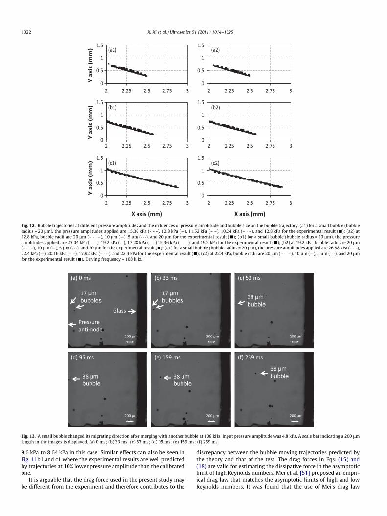
Fig. 13. A small bubble changed its migrating direction after merging with another bubble at 108 kHz. Input pressure amplitude was 4.8 kPa. A scale bar indicating a 200 lmlength in the images is displayed. (a) 0 ms; (b) 33 ms; (c) 53 ms; (d) 95 ms; (e) 159 ms; (f) 259 ms.

Fig. 12. Bubble trajectories at different pressure amplitudes and the influences of pressure amplitude and bubble size on the bubble trajectory. (a1) for a small bubble (bubbleradius = 20 lm), the pressure amplitudes applied are 15.36 kPa (- - -), 12.8 kPa (—), 11.52 kPa (– –), 10.24 kPa (– � –), and 12.8 kPa for the experimental result (j); (a2) at12.8 kPa, bubble radii are 20 lm (– � � –), 10 lm (—), 5 lm (� � �), and 20 lm for the experimental result (j); (b1) for a small bubble (bubble radius = 20 lm), the pressureamplitudes applied are 23.04 kPa (- - -), 19.2 kPa (—), 17.28 kPa (– –) 15.36 kPa (– � –), and 19.2 kPa for the experimental result (j); (b2) at 19.2 kPa, bubble radii are 20 lm(– � � –), 10 lm (—), 5 lm (� � �), and 20 lm for the experimental result (j); (c1) for a small bubble (bubble radius = 20 lm), the pressure amplitudes applied are 26.88 kPa (- - -),22.4 kPa (—), 20.16 kPa (– –), 17.92 kPa (– � –), and 22.4 kPa for the experimental result (j); (c2) at 22.4 kPa, bubble radii are 20 lm (– � � –), 10 lm (—), 5 lm (� � �), and 20 lmfor the experimental result (j). Driving frequency = 108 kHz.

1022 X. Xi et al. / Ultrasonics 51 (2011) 1014–1025

9.6 kPa to 8.64 kPa in this case. Similar effects can also be seen inFig. 11b1 and c1 where the experimental results are well predictedby trajectories at 10% lower pressure amplitude than the calibratedone.

It is arguable that the drag force used in the present study maybe different from the experiment and therefore contributes to the

discrepancy between the bubble moving trajectories predicted bythe theory and that of the test. The drag forces in Eqs. (15) and(18) are valid for estimating the dissipative force in the asymptoticlimit of high Reynolds numbers. Mei et al. [51] proposed an empir-ical drag law that matches the asymptotic limits of high and lowReynolds numbers. It was found that the use of Mei’s drag law

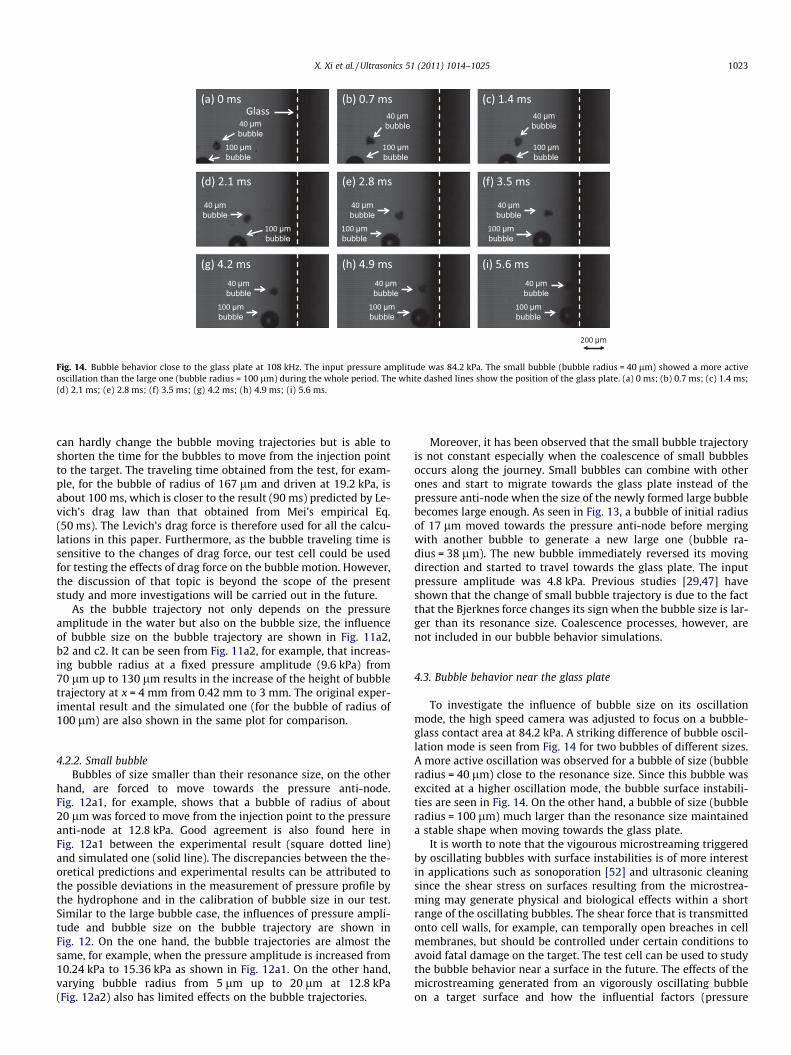
Fig. 14. Bubble behavior close to the glass plate at 108 kHz. The input pressure amplitude was 84.2 kPa. The small bubble (bubble radius = 40 lm) showed a more activeoscillation than the large one (bubble radius = 100 lm) during the whole period. The white dashed lines show the position of the glass plate. (a) 0 ms; (b) 0.7 ms; (c) 1.4 ms;(d) 2.1 ms; (e) 2.8 ms; (f) 3.5 ms; (g) 4.2 ms; (h) 4.9 ms; (i) 5.6 ms.

X. Xi et al. / Ultrasonics 51 (2011) 1014–1025 1023

can hardly change the bubble moving trajectories but is able toshorten the time for the bubbles to move from the injection pointto the target. The traveling time obtained from the test, for exam-ple, for the bubble of radius of 167 lm and driven at 19.2 kPa, isabout 100 ms, which is closer to the result (90 ms) predicted by Le-vich’s drag law than that obtained from Mei’s empirical Eq.(50 ms). The Levich’s drag force is therefore used for all the calcu-lations in this paper. Furthermore, as the bubble traveling time issensitive to the changes of drag force, our test cell could be usedfor testing the effects of drag force on the bubble motion. However,the discussion of that topic is beyond the scope of the presentstudy and more investigations will be carried out in the future.

As the bubble trajectory not only depends on the pressureamplitude in the water but also on the bubble size, the influenceof bubble size on the bubble trajectory are shown in Fig. 11a2,b2 and c2. It can be seen from Fig. 11a2, for example, that increas-ing bubble radius at a fixed pressure amplitude (9.6 kPa) from70 lm up to 130 lm results in the increase of the height of bubbletrajectory at x = 4 mm from 0.42 mm to 3 mm. The original exper-imental result and the simulated one (for the bubble of radius of100 lm) are also shown in the same plot for comparison.

4.2.2. Small bubbleBubbles of size smaller than their resonance size, on the other

hand, are forced to move towards the pressure anti-node.Fig. 12a1, for example, shows that a bubble of radius of about20 lm was forced to move from the injection point to the pressureanti-node at 12.8 kPa. Good agreement is also found here inFig. 12a1 between the experimental result (square dotted line)and simulated one (solid line). The discrepancies between the the-oretical predictions and experimental results can be attributed tothe possible deviations in the measurement of pressure profile bythe hydrophone and in the calibration of bubble size in our test.Similar to the large bubble case, the influences of pressure ampli-tude and bubble size on the bubble trajectory are shown inFig. 12. On the one hand, the bubble trajectories are almost thesame, for example, when the pressure amplitude is increased from10.24 kPa to 15.36 kPa as shown in Fig. 12a1. On the other hand,varying bubble radius from 5 lm up to 20 lm at 12.8 kPa(Fig. 12a2) also has limited effects on the bubble trajectories.

Moreover, it has been observed that the small bubble trajectoryis not constant especially when the coalescence of small bubblesoccurs along the journey. Small bubbles can combine with otherones and start to migrate towards the glass plate instead of thepressure anti-node when the size of the newly formed large bubblebecomes large enough. As seen in Fig. 13, a bubble of initial radiusof 17 lm moved towards the pressure anti-node before mergingwith another bubble to generate a new large one (bubble ra-dius = 38 lm). The new bubble immediately reversed its movingdirection and started to travel towards the glass plate. The inputpressure amplitude was 4.8 kPa. Previous studies [29,47] haveshown that the change of small bubble trajectory is due to the factthat the Bjerknes force changes its sign when the bubble size is lar-ger than its resonance size. Coalescence processes, however, arenot included in our bubble behavior simulations.

4.3. Bubble behavior near the glass plate

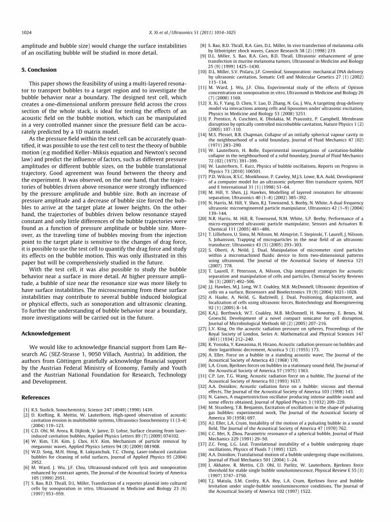
To investigate the influence of bubble size on its oscillationmode, the high speed camera was adjusted to focus on a bubble-glass contact area at 84.2 kPa. A striking difference of bubble oscil-lation mode is seen from Fig. 14 for two bubbles of different sizes.A more active oscillation was observed for a bubble of size (bubbleradius = 40 lm) close to the resonance size. Since this bubble wasexcited at a higher oscillation mode, the bubble surface instabili-ties are seen in Fig. 14. On the other hand, a bubble of size (bubbleradius = 100 lm) much larger than the resonance size maintaineda stable shape when moving towards the glass plate.

It is worth to note that the vigourous microstreaming triggeredby oscillating bubbles with surface instabilities is of more interestin applications such as sonoporation [52] and ultrasonic cleaningsince the shear stress on surfaces resulting from the microstrea-ming may generate physical and biological effects within a shortrange of the oscillating bubbles. The shear force that is transmittedonto cell walls, for example, can temporally open breaches in cellmembranes, but should be controlled under certain conditions toavoid fatal damage on the target. The test cell can be used to studythe bubble behavior near a surface in the future. The effects of themicrostreaming generated from an vigorously oscillating bubbleon a target surface and how the influential factors (pressure

1024 X. Xi et al. / Ultrasonics 51 (2011) 1014–1025

amplitude and bubble size) would change the surface instabilitiesof an oscillating bubble will be studied in more detail.

5. Conclusion

This paper shows the feasibility of using a multi-layered resona-tor to transport bubbles to a target region and to investigate thebubble behavior near a boundary. The designed test cell, whichcreates a one-dimensional uniform pressure field across the crosssection of the whole stack, is ideal for testing the effects of anacoustic field on the bubble motion, which can be manipulatedin a very controlled manner since the pressure field can be accu-rately predicted by a 1D matrix model.

As the pressure field within the test cell can be accurately quan-tified, it was possible to use the test cell to test the theory of bubblemotion (e.g modified Keller–Miksis equation and Newton’s secondlaw) and predict the influence of factors, such as different pressureamplitudes or different bubble sizes, on the bubble translationaltrajectory. Good agreement was found between the theory andthe experiment. It was observed, on the one hand, that the trajec-tories of bubbles driven above resonance were strongly influencedby the pressure amplitude and bubble size. Both an increase ofpressure amplitude and a decrease of bubble size forced the bub-bles to arrive at the target plate at lower heights. On the otherhand, the trajectories of bubbles driven below resonance stayedconstant and only little differences of the bubble trajectories werefound as a function of pressure amplitude or bubble size. More-over, as the traveling time of bubbles moving from the injectionpoint to the target plate is sensitive to the changes of drag force,it is possible to use the test cell to quantify the drag force and studyits effects on the bubble motion. This was only illustrated in thispaper but will be comprehensively studied in the future.

With the test cell, it was also possible to study the bubblebehavior near a surface in more detail. At higher pressure ampli-tude, a bubble of size near the resonance size was more likely tohave surface instabilities. The microscreaming from these surfaceinstabilities may contribute to several bubble induced biologicalor physical effects, such as sonoporation and ultrasonic cleaning.To further the understanding of bubble behavior near a boundary,more investigations will be carried out in the future.

Acknowledgement

We would like to acknowledge financial support from Lam Re-search AG (SEZ-Strasse 1, 9050 Villach, Austria). In addition, theauthors from Göttingen gratefully acknowledge financial supportby the Austrian Federal Ministry of Economy, Family and Youthand the Austrian National Foundation for Research, Technologyand Development.

References

[1] K.S. Suslick, Sonochemistry, Science 247 (4949) (1990) 1439.[2] D. Krefting, R. Mettin, W. Lauterborn, High-speed observation of acoustic

cavitation erosion in multibubble systems, Ultrasonics Sonochemistry 11 (3–4)(2004) 119–123.

[3] C.D. Ohl, M. Arora, R. Dijkink, V. Janve, D. Lohse, Surface cleaning from laser-induced cavitation bubbles, Applied Physics Letters 89 (7) (2009) 074102.

[4] W. Kim, T.H. Kim, J. Choi, H.Y. Kim, Mechanism of particle removal bymegasonic waves, Applied Physics Letters 94 (8) (2009) 081908.

[5] W.D. Song, M.H. Hong, B. Lukyanchuk, T.C. Chong, Laser-induced cavitationbubbles for cleaning of solid surfaces, Journal of Applied Physics 95 (2004)2952.

[6] M. Ward, J. Wu, J.F. Chiu, Ultrasound-induced cell lysis and sonoporationenhanced by contrast agents, The Journal of the Acoustical Society of America105 (1999) 2951.

[7] S. Bao, B.D. Thrall, D.L. Miller, Transfection of a reporter plasmid into culturedcells by sonoporation in vitro, Ultrasound in Medicine and Biology 23 (6)(1997) 953–959.

[8] S. Bao, B.D. Thrall, R.A. Gies, D.L. Miller, In vivo transfection of melanoma cellsby lithotripter shock waves, Cancer Research 58 (2) (1998) 219.

[9] D.L. Miller, S. Bao, R.A. Gies, B.D. Thrall, Ultrasonic enhancement of genetransfection in murine melanoma tumors, Ultrasound in Medicine and Biology25 (9) (1999) 1425–1430.

[10] D.L. Miller, S.V. Pislaru, J.F. Greenleaf, Sonoporation: mechanical DNA deliveryby ultrasonic cavitation, Somatic Cell and Molecular Genetics 27 (1) (2002)115–134.

[11] M. Ward, J. Wu, J.F. Chiu, Experimental study of the effects of Optisonconcentration on sonoporation in vitro, Ultrasound in Medicine and Biology 26(7) (2000) 1169.

[12] X. Xi, F. Yang, D. Chen, Y. Luo, D. Zhang, N. Gu, J. Wu, A targeting drug-deliverymodel via interactions among cells and liposomes under ultrasonic excitation,Physics in Medicine and Biology 53 (2008) 3251.

[13] P. Prentice, A. Cuschieri, K. Dholakia, M. Prausnitz, P. Campbell, Membranedisruption by optically controlled microbubble cavitation, Nature Physics 1 (2)(2005) 107–110.

[14] M.S. Plesset, R.B. Chapman, Collapse of an initially spherical vapour cavity inthe neighbourhood of a solid boundary, Journal of Fluid Mechanics 47 (02)(1971) 283–290.

[15] W. Lauterborn, H. Bolle, Experimental investigations of cavitation-bubblecollapse in the neighbourhood of a solid boundary, Journal of Fluid Mechanics72 (02) (1975) 391–399.

[16] W. Lauterborn, T. Kurz, Physics of bubble oscillations, Reports on Progress inPhysics 73 (2010) 106501.

[17] P.D. Wilcox, R.S.C. Monkhouse, P. Cawley, M.J.S. Lowe, B.A. Auld, Developmentof a computer model for an ultrasonic polymer film transducer system, NDTand E International 31 (1) (1998) 51–64.

[18] M. Hill, Y. Shen, J.J. Hawkes, Modelling of layered resonators for ultrasonicseparation, Ultrasonics 40 (1–8) (2002) 385–392.

[19] N. Harris, M. Hill, Y. Shen, R.J. Townsend, S. Beeby, N. White, A dual frequencyultrasonic microengineered particle manipulator, Ultrasonics 42 (1–9) (2004)139–144.

[20] N.R. Harris, M. Hill, R. Townsend, N.M. White, S.P. Beeby, Performance of amicro-engineered ultrasonic particle manipulator, Sensors and Actuators B:Chemical 111 (2005) 481–486.

[21] T. Lilliehorn, U. Simu, M. Nilsson, M. Almqvist, T. Stepinski, T. Laurell, J. Nilsson,S. Johansson, Trapping of microparticles in the near field of an ultrasonictransducer, Ultrasonics 43 (5) (2005) 293–303.

[22] S. Oberti, A. Neild, J. Dual, Manipulation of micrometer sized particleswithin a micromachined fluidic device to form two-dimensional patternsusing ultrasound, The Journal of the Acoustical Society of America 121(2007) 778.

[23] T. Laurell, F. Petersson, A. Nilsson, Chip integrated strategies for acousticseparation and manipulation of cells and particles, Chemical Society Reviews36 (3) (2007) 492–506.

[24] J.J. Hawkes, M.J. Long, W.T. Coakley, M.B. McDonnell, Ultrasonic deposition ofcells on a surface, Biosensors and Bioelectronics 19 (9) (2004) 1021–1028.

[25] A. Haake, A. Neild, G. Radziwill, J. Dual, Positioning, displacement, andlocalization of cells using ultrasonic forces, Biotechnology and Bioengineering92 (1) (2005) 8–14.

[26] K.A.J. Borthwick, W.T. Coakley, M.B. McDonnell, H. Nowotny, E. Benes, M.Groeschl, Development of a novel compact sonicator for cell disruption,Journal of Microbiological Methods 60 (2) (2005) 207–216.

[27] L.V. King, On the acoustic radiation pressure on spheres, Proceedings of theRoyal Society of London, Series A: Mathematical and Physical Sciences 147(861) (1934) 212–240.

[28] K. Yosioka, Y. Kawasima, H. Hirano, Acoustic radiation pressure on bubbles andtheir logarithmic decrement, Acustica 5 (3) (1955) 173.

[29] A. Eller, Force on a bubble in a standing acoustic wave, The Journal of theAcoustical Society of America 43 (1968) 170.

[30] L.A. Crum, Bjerknes forces on bubbles in a stationary sound field, The Journal ofthe Acoustical Society of America 57 (1975) 1363.

[31] C.P. Lee, T.G. Wang, Acoustic radiation force on a bubble, The Journal of theAcoustical Society of America 93 (1993) 1637.

[32] A.A. Doinikov, Acoustic radiation force on a bubble: viscous and thermaleffects, The Journal of the Acoustical Society of America 103 (1998) 143.

[33] N. Gaines, A magnetostriction oscillator producing intense audible sound andsome effects obtained, Journal of Applied Physics 3 (1932) 209–229.

[34] M. Strasberg, T.B. Benjamin, Excitation of oscillations in the shape of pulsatinggas bubbles: experimental work, The Journal of the Acoustical Society ofAmerica 30 (1958) 697.

[35] A.I. Eller, L.A. Crum, Instability of the motion of a pulsating bubble in a soundfield, The Journal of the Acoustical Society of America 47 (1970) 762.

[36] C.C. Mei, X. Zhou, Parametric resonance of a spherical bubble, Journal of FluidMechanics 229 (1991) 29–50.

[37] Z.C. Feng, L.G. Leal, Translational instability of a bubble undergoing shapeoscillations, Physics of Fluids 7 (1995) 1325.

[38] A.A. Doinikov, Translational motion of a bubble undergoing shape oscillations,Journal of Fluid Mechanics 501 (2004) 1–24.

[39] I. Akhatov, R. Mettin, C.D. Ohl, U. Parlitz, W. Lauterborn, Bjerknes forcethreshold for stable single bubble sonoluminescence, Physical Review E 55 (3)(1997) 3747–3750.

[40] T.J. Matula, S.M. Cordry, R.A. Roy, L.A. Crum, Bjerknes force and bubblelevitation under single-bubble sonoluminescence conditions, The Journal ofthe Acoustical Society of America 102 (1997) 1522.

X. Xi et al. / Ultrasonics 51 (2011) 1014–1025 1025

[41] D.L. Miller, Stable arrays of resonant bubbles in a 1-MHz standing-waveacoustic field, The Journal of the Acoustical Society of America 62 (1977) 12.

[42] S. Khanna, N.N. Amso, S.J. Paynter, W.T. Coakley, Contrast agent bubble anderythrocyte behavior in a 1.5-MHz standing ultrasound wave, Ultrasound inMedicine and Biology 29 (10) (2003) 1463–1470.

[43] L.A. Kuznetsova, S. Khanna, N.N. Amso, W.T. Coakley, A.A. Doinikov, Cavitationbubble-driven cell and particle behavior in an ultrasound standing wave, TheJournal of the Acoustical Society of America 117 (2005) 104.

[44] Y. Abe, M. Kawaji, T. Watanabe, Study on the bubble motion control byultrasonic wave, Experimental Thermal and Fluid Science 26 (6–7) (2002)817–826.

[45] T. Watanabe, Y. Kukita, Translational and radial motions of a bubble in anacoustic standing wave field, Physics of Fluids A: Fluid Dynamics 5 (1993)2682.

[46] A.A. Doinikov, Translational motion of a spherical bubble in an acousticstanding wave of high intensity, Physics of Fluids 14 (2002) 1420.

[47] R. Mettin, A.A. Doinikov, Translational instability of a spherical bubble in astanding ultrasound wave, Applied Acoustics 70 (10) (2009) 1330–1339.

[48] J.B. Keller, M. Miksis, Bubble oscillations of large amplitude, The Journal of theAcoustical Society of America 68 (2) (1980) 628–633.

[49] U. Parlitz, V. Englisch, C. Scheffczyk, W. Lauterborn, Bifurcation structure ofbubble oscillators, The Journal of the Acoustical Society of America 88 (2)(1990) 1061–1077.

[50] T.G. Leighton, The Acoustic Bubble, Academic Press, 1997.[51] R. Mei, J.F. Klausner, C.J. Lawrence, A note on the history force on a spherical

bubble at finite reynolds number, Physics of Fluids 6 (1994) 418.[52] J. Wu, J.P. Ross, J.F. Chiu, Reparable sonoporation generated by microstreaming,

The Journal of the Acoustical Society of America 111 (2002) 1460.