Studying and Verifying the Use of ChemicalBiomarkers for Identifying and QuantitatingOil Residues in the Environment

U.S. Deoartment of the InteriorMinerals )Aanagement ServiceGulf of Mexico OCS Region

30

Cooperative AgreementCoastal Marine InstituteLouisiana State University

OCS StudyMMS 2000-086

Coastal Marine Institute

Coastal Marine Institute

Studying and Verifying the Use of ChemicalBiomarkers for Identifying and QuantitatingOil Residues in the Environment

Authors

Buffy M. AshtonRebecca S. EastMaud M. WalshM. Scott MilesEdward B. OvertonInstitute for Environmental SciencesLouisiana State UniversityBaton Rouge, Louisiana

December 2000

Prepared under MMS Contract14-35-0001-30660-19933byCoastal Marine InstituteLouisiana State UniversityRoom 318 Howe-RussellBaton Rouge, Louisiana 70801

Published by

U.S. Department of the InteriorMinerals Management ServiceGulf of Mexico OCS Region

OCS StudyMMS 2000-086

Cooperative AgreementCoastal Marine InstituteLouisiana State University

DISCLAIMER

This report was prepared under contract between the Minerals Management Service(MMS) and Louisiana State University, Institute for Environmental Studies. This reporthas been reviewed by the MMS and approved for publication. Approval does not signifythat the contents necessarily reflect the views and policies of the Service, nor doesmention of trade names or commercial products constitute endorsement orrecommendation for use. It is, however, exempt from review and compliance with MMSeditorial standards.

REPORT AVAILABILITY

Extra copies of the report may be obtained from the Public Information Unit (Mail Stop5034) at the following address

U.S. Department of the InteriorMinerals Management ServiceGulf of Mexico OCS Regional OfficeAttention: Public Information Unit (MS 5034)1201 Elmwood Park BoulevardNew Orleans, Louisiana 70123-2394

Telephone Number: (504) 736-2519 or1 -800-200-GULF

CITATION

Suggested citation:

Ashton, B.M., R.S. East, M..M. Walsh, M.S. Miles, and E.B. Overton. 2000. Studyingand Verif'ing the Use of Chemical Biomarkers for Identi'ing and QuantitatingOil Residues in the Environment. U.S. Dept. of the Interior, MineralsManagement Service, Gulf of Mexico OCS Region, New Orleans, LA.OCS Study MMS 2000-086. 70 pp.

ACKNOWLEDGEMENTS

The authors would like to acknowledge and thank the many people who participated inthe funding, collection, and analytical phases of this research. Extra special thanks areextended to Charlie Henry and Paulene Roberts who began the preliminary stages of theexperimental design and assisted in the collection and preliminary data interpretations.Their knowledge, guidance, and suggestions were invaluable. Shane Bourke assisted insample collection. Ron LeBlanc helped with the sample preparation and analysis. Thankyou James Welch, Donny Blanchard, David Brown, Jermifer Betbeze, and Barrett Ortegofor your time and help with the data processing.

111

ABSTRACT

Analytical chemistiy and instrumentation provides environmental scientists with theability to identify and track the fate of spilled oil residues in the marine environmentCompounds commonly used for the identification of spilled oil to a source are calledbiomarkers. Biomarker compounds are universal in crude oils and petroleum productsand are generally more resistant to environmental weathering than most other oilconstituents. The distribution of biomarker compounds is unique for each oil anddifferent sources of petroleum exhibit different oil fingerprints. Self-normalizingfingerprint indexes (SF1) calculated from the oil fingerprints provide a stable and usefultool for determining a match or nonmatch for different oil residues present in someenvironmental samples. A combination high-resolution gas chromatography and massspectrometry, visual comparison and self-normalizing fingerprint indexes (SF1) wereutilized to establish eight petroleum biomarkers for oil spill identification and assessment.

The eight petroleum biomarkers chosen for detection and analysis were determinedthrough a literature search and previous research. SF1 calculated from GC/MS analysisof tarballs and an oil degradation study validated the use of the eight biomarkers chosen.Of the eight SF1, four remain stable over an extended period of time and laboratorysimulated weathering. Visual comparison of biomarker fingerprints played an importantrole in distinguishing gross, and in some cases subtle, differences between unknownenvironmental samples. Double SF1 scatterplots were also utilized as a screening tool forsource matchlnonmatch determinations.

v

TABLE OF CONTENTS

ABSTRACT

LIST OF FIGURES ix

LIST OF TABLES xi

INTRODUCTION 1

Research Objective 1

Background Information 1

Biomarkers 3Analytical Chemistry and Oil Characterization - 5

Self-Normalizing Fingerprint Indexes 8Project Goals 9

Preliminary Stages 13

Laboratory-Simulated Weathering and Degradation Study 14Bioaccumulation 15

Classification and Identification of Tarballs 15

METHODOLOGY 16General Laboratory Methodology 16

GCIMS Methodology 16Calculation of SF1 17

Visual Matching 17

Laboratory-Simulated Weathering and Degradation Study 18

Bioaccumulation 19Classification and Identification of Tarballs 20

RESULTS AND DISCUSSION 23Laboratory-Simulated Weathering and Degradation Study 23Bioaccumulation 30Classification and Identification of Tarballs 32

Morphological Appearance 34Analytical Chemistry Results 38Visual Matching 39SF1 and Scatterplots 47

CONCLUSIONS AND RECOMMENDATIONS 49

LITERATURE CITED 53

APPENDIX. Biomarkers of Petroleum Products in the Marine Environment: ABibliography 57

VII

LIST OF FIGURES

Structures of triterpanes and steranes, both common biomarker compounds 4

Other oil biomarker compounds dibenzothiophene; phenanthrene; chrysene;and pyrene

Extracted ion chromatogram indicating C-17/Pristane and C-18/Phytane SF1 10

Extracted ion chromatogram indicating C-3 DBT (a/b) SF1 10

Extracted ion chromatogram indicating C-3 Phen (a/b) SF1 11

Extracted ion chromatogram indicating C-i Pyr (a/b) SF1 ii

Extracted ion chromatogram indicating C-i Chr (a/b) SF1 i2

Extracted ion chromatogram indicating Norhopane/Hopane SF1 12

Sampling locations along the Louisiana coastline for stranded oil and tar survey,1998 21

Average TTAH for each site and two controls 24

Total sources utilized by microorganisms from BiologTM results 26

Percent aromatic chemicals utilized by microorganisms from Biologm results 26

Total polycyclic aromatic hydrocarbons (PAHs) and biomarker concentrations inFl fractions from mussel tissues 31

Total polycyclic aromatic hydrocarbons (PAHs) and biomarker concentrations inFl fractions from clam tissues 31

Surface color distribution of tarballs collected in 1998 survey 35

Inside color distribution for tarballs collected in 1998 survey 35

Percent organic matter distribution for tarballs collected in 1998 survey 36

Percent sand distribution for tarballs collected in 1998 survey 36

Percent shell distribution for tarballs collected in 1998 survey 37

Tarball pliability score for 1998 samples 37

ix

LIST OF FIGURES(CONTINUED)

Normal alkane distribution and Total Ion Chromatogram for a relativelyunweathered, aromatic oil 40

Normal alkane distribution and Total Ion Chromatogram for a relativelyunweathered, paraffinic oil 41

Normal alkane distribution and Total Ion Chromatogram for a relativelyunweathered, bimodal wax 42

Normal alkane distribution and Total Ion Chromatogram for a weathered,aromatic oil 43

Normal alkane distribution and Total Ion Chromatogram for a weathered,paraffinic oil 44

Normal alkane distribution and Total Ion Chromatogram for a weathered,bimodal wax

Normal alkane distribution and Total Ion Chromatogram for a weathered, 11CM

C3 Phenanthrene versus C3 Dibenzothiophene/C3 Phenanthrene area double SF1scatterplot for tarballs from Martin's beach 48

Norhopane/Hopane versus C3 Dibenzothiophene/C3 Phenanthrene area doubleSF1 scatterplot for tarballs from Martin's beach 48

Suggested method for match/nonmatch determinations of unknown environmentaloil samples to a reference oil based on visual comparison and SF1 data 51

x

45

46

LIST OF TABLES

Target Petroleum Biomarkers 4

List of Target Oil Constituents Analyzed for by GC/MS-SIM in the IES/RCATLaboratory 7

List of Keywords Utilized in the Literature Search 13

SIM Ion Grouping for Target Crude Oil Compounds 17

Percent of TTAH Reduction for the Nine Water Samples After 28-Day WeatheringExperiment 23

Physical Characteristic Data and % Reduction in TTAH for Water Samples Basedon the Experimental Location Average Temperature 27

SF1 Data and Statistical Results for All Collection Sites, Without Nutrients 27

SF1 Data and Statistical Results for All Collection Sites, With Nutrients 28

SF1 Data and Statistical Results for Daily ETC Reference Oil 28

SF1 Profiles for Fourteen Reference Oils 32

Distribution of All Tarballs into Classifications 39

xi

INTRODUCTION

Research Objective

Analytical chemistry and instrumentation provides environmental scientists with the ability toidenti& and track the fate of spilled oil residues in the marine environment. Since the 1960'smany advances have been made in analytical chemistry techniques and instrumentation;however, despite these advances, more accurate methods are necessary for identiing andquantif'ing oil contamination in the environment. Biomarkers, for the purpose of this study,are petroleum components that remain relatively unchanged in oil residues even after naturalenvironmental weathering processes. Since these biomarker compounds are relativelypersistent, they are commonly used for the identification of a spilled oil to its source. Theobjective of this research is to refine the use of biomarkers as tools for oil spill identificationand assessment, and to veri' the analytical approach utilized by the Louisiana StateUniversity, Institute for Environmental Studies, Response and Chemical Assessment Team(LSU IES/RCAT) with both laboratory and field evaluation studies. High-resolution gaschromatography and mass spectrometry (GC/MS) and source-fingerprinting techniques will beemployed to fulfill the research objective. Visual comparison, self-normalizing fingerprintindexes (SF1) calculated from GCIMS analysis and biomarker normalization methods willprovide further validation for the importance of analyzing biomarkers in oil and oil residuesfound in the marine environment.

Background Information

Oil spills into marine environments have been recognized as major environmental insults formore than 30 years. The 1968 Torrey Canyon spill accentuated the large volumes of oil andpotential environmental threat posed by the then newly introduced "supertanker." In 1969, aproduction well blow-out off the California coastal city of Santa Barbara caused another majorspill in the marine environment further highlighting environmental concerns generated by oilpollution. Since the 1960s, there have been numerous spills around the world, including theinfamous Amoco Cadiz and Exxon Valdez spills, as well as major well blow-outs in the NorthSea, Bay of Campeche, and the Persian Gulf Tn addition to these incidents, intentional oil firesand marine oil spills which occurred during the 1991 Persian Gulf War have also contributed toenvironmental contamination and resulted in considerable media attention. Media attentionoften leads to public outrage and in some cases, such as in the United States following theExxon Valdez, laws are created and passed to control and give liability to the responsible parties(i.e. The Oil Pollution Act of 1990).

High profile oil spills are not the only source of oil pollution in marine and other environments.Chronic oil discharges occur from a variety of small spills, natural seeps of oil from rivers andoceans, non-point source mn-off, operational discharges from tankers, and developmentassociated with petroleum exploration. As a result, there is approximately 5 million tons of oilreleased into the oceans each year. Approximately 6% of the 5 million tons (300,000) are fromtanicer accidents such as the Exxon Valdez, while the remaining 4.7 million tons are fromnatural, chronic and acute events (Henry 1995).

1

Crude oil is a complex mixture of organic compounds derived from the partial decompositionof animals and plants that were once alive, but have been long since dead. The process of oilformation occurs slowly and produces "simple" organic molecules (petroleum) from morecomplex organic structures (organic biomass). Petroleum-type hydrocarbons may exist as a gas(natural gas), as a liquid (crude oil), as a solid (tar, bitumen), or any combination. All crudeoils are composed primarily of carbon (80-87%) and hydrogen (10-15%), and to a lesserdegree, sulfur (0-10%), nitrogen (0-1%) and oxygen (0-0.5%). Metals are a minor constituentin petroleum and contribute little to the toxicity of oil. The physical and chemical properties ofcrude oil vary with regions of production and zones within these regions. Since crude oils vary,no single definition or composition is valid for all oils.

In general, all crude oils tend to be composed of the same individual compounds but therelative abundance of these compounds may vary significantly between different oils. Thesedifferences are important from the refinery processing and environmental chemistry perspectivebecause they are useful for predicting how an oil will behave if spilled in the marineenvironment. Common oil constituents can be classified into four general groups: (1)individual saturated hydrocarbons (the normal alkanes and isoprenoids); (2) polycyclicaromatic hydrocarbons (PAils) including the dominant alkylated homologues in oil; (3) sulfurheterocyclic aromatic hydrocarbons and related alkylated homologues; and (4) oil biomarkers(primarily the steranes and triterpanes) which are polycyclic aliphatics. Even though aromatichydrocarbons (groups 2, 3, and 4) represent less than 5% of the bulk composition of most oils,they are essential for assessing biological effects, aid in determining exposure pathways, sourcecharacterization, and for monitoring the extent of oil weathering and degradation (Sauer andBoehm 1991).

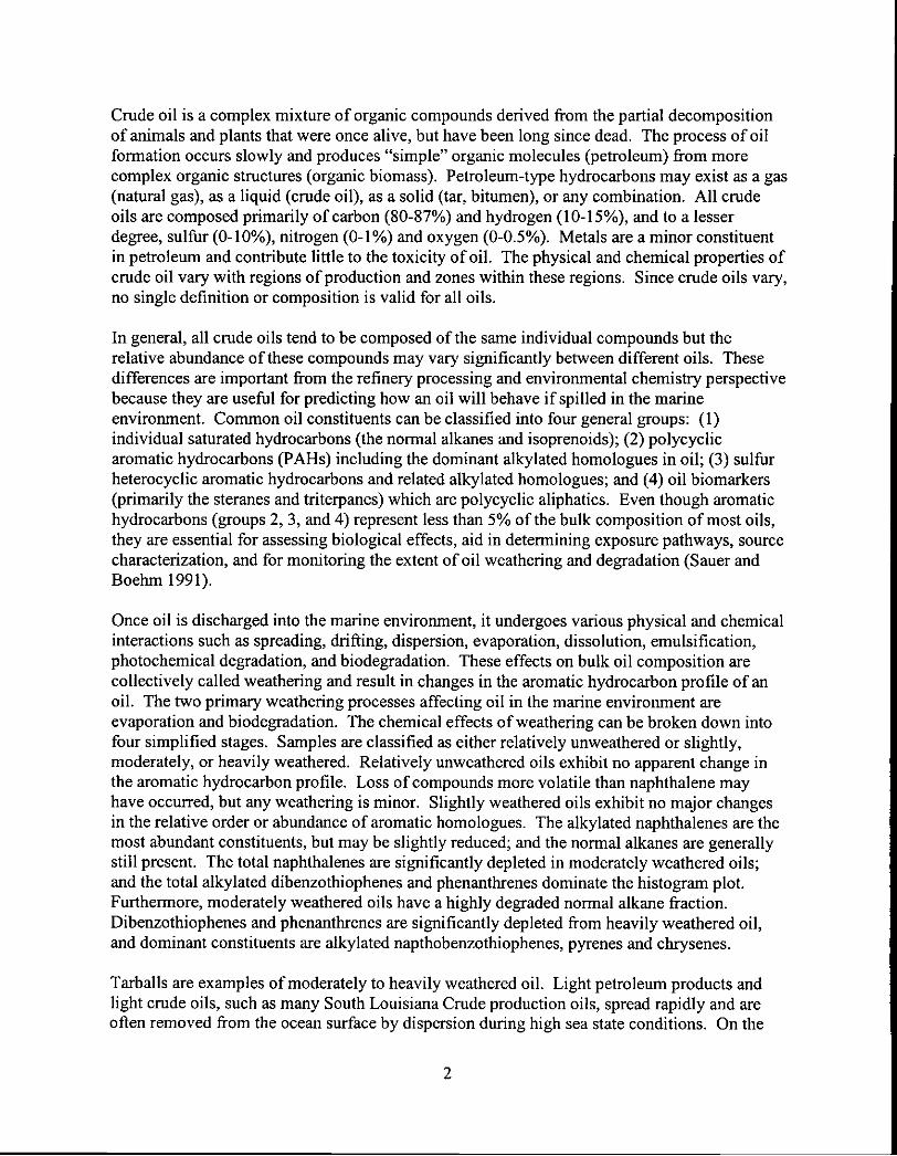
Once oil is discharged into the marine environment, it undergoes various physical and chemicalinteractions such as spreading, drifting, dispersion, evaporation, dissolution, emulsification,photochemical degradation, and biodegradation. These effects on bulk oil composition arecollectively called weathering and result in changes in the aromatic hydrocarbon profile of anoil. The two primary weathering processes affecting oil in the marine environment areevaporation and biodegradation. The chemical effects of weathering can be broken down intofour simplified stages. Samples are classified as either relatively unweathered or slightly,moderately, or heavily weathered. Relatively unweathered oils exhibit no apparent change inthe aromatic hydrocarbon profile. Loss of compounds more volatile than naphthalene mayhave occurred, but any weathering is minor. Slightly weathered oils exhibit no major changesin the relative order or abundance of aromatic homologues. The alkylated naphthalenes are themost abundant constituents, but may be slightly reduced; and the normal alkanes are generallystill present. The total naphthalenes are significantly depleted in moderately weathered oils;and the total alkylated dibenzothiophenes and phenanthrenes dominate the histogram plot.Furthermore, moderately weathered oils have a highly degraded normal alkane fraction.Dibenzothiophenes and phenanthrenes are significantly depleted from heavily weathered oil,and dominant constituents are alkylated napthobenzothiophenes, pyrenes and chrysenes.

Tarballs are examples of moderately to heavily weathered oil. Light petroleum products andlight crude oils, such as many South Louisiana Crude production oils, spread rapidly and areoften removed from the ocean surface by dispersion during high sea state conditions. On the

2

other hand, the very heavy crude oils, refined heavy bunker oils, and other petroleum productswith high pour points are slow to spread, exposing little surface area for the natural degradationprocess. Thick oils are generally only degraded at the surface interface resulting in theencapsulation of "fresher" oil. As a result, heavier oils are the most persistent in theenvironment and are often encountered as stranded tarballs along the debris line of the beachface. The formation of "mousse", a stable water-in-oil emulsification, may enhance theprocess of tarball formation and extend environmental persistence of the lighter crude oils.Mousse formation is common and is a prime factor for the formation of tarballs from otherwiseeasily dispersible light crude oils.

Factors that influence weathering include weather conditions, the environment in which the oilwas spilled, and the type of oil. Once oil is stranded on a beach or shoreline, weathering ismodified by the microenvironment in which the oil is entrapped and the rate of naturalbiodegradation at any specific location is dependent on a variety of factors. The amount of oil,mixing energy, microfauna, and the availability of oxygen are a few of the key factors ofbiodegradation. The limiting factor is often the availability of oil to the microbial community.Other physical/chemical properties that affect the fate of individual constituents in crude oilinclude vapor pressure, water solubility, the organic carbon partitioning coefficient (K0) andoctanol/water partitioning coefficients (}Q). Different oils spilled under similar conditionsmay undergo entirely different weathering changes. The ability to examine a sample ofresidual oil (such as a tarball) and speculate on the composition of the unweathered oil fromwhich it was derived is valuable information. Environmental forensic investigations todetermine a potential source of an unknown or mystery spill must exploit both morphological,as well as, chemical compositional differences.

Biomarkers

As previously stated, petroleum spilled into the marine environment undergoes varying degreesof environmental weathering that affect its composition. As weathering proceeds, certaingroups of oil constituents are lost in a predictable sequence. The first compounds to bedepleted are the n-alkanes and isoprenoids, followed by the lighter PAHs, then the remainingPAHs and their alkyl homologues. As a result, unique identification of sources of oil spillsmay be difficult due to the loss of these oil constituents and their distribution patterns relativeto the amount of weathering.

Biomarkers, as defined for this research, are petroleum components that remain detectable andrelatively unchanged in oil residues even after natural environmental weathering processes.They are also typically resistant to biodegradation and are therefore, usefifi as chemicalmarkers. Biomarker fingerprinting by (iC/MS may be necessary for environmental samples inwhich identification of spilled oil is difficult due to weathering of target compounds. Twoclasses of biomarkers commonly referred to in the literature are the triterpane and steranecompounds (Figure 1). The triterpane and sterane distributions are unique for each type of oil,and, because of their relatively refractory nature, these compounds help to identif' a particularoil, even oils with similar geographical origins, when other target analytes are lost. Biomarkerssuffer little interference from weathering effects because of their high resistance to degradation,which can be attributed to their high molecular weights. As an oil becomes more degraded, the

3

concentration of biomarker compounds should increase relative to the more easily degradedconstituents (Wang and Fingas 1995b). These compounds are also useful in distinguishing aspilled oil from other oils and sources that may be present within the same sample matrix. As aresult, biomarkers provide chemical fingerprinting information about the source, degree ofweathering, characteristics, and fate of the spilled oil.

Figure 1. Structures of (a) triterpanes and(b) steranes, both common biomarkercompounds.

While the hopanes and steranes are useful biornarker compounds, other biomarkers from one ofthe four groups of oil constituents previously listed are essential due to the fact that refineryprocesses remove the triterpanes and steranes. Previous research in the IES/RCAT laboratory,as well as other studies reported in the literature, suggest that the compounds and ratios listed inTable 1 are most promising as biomarkers. The "n" represents normal alkane (rn/c 85), and"C" relates to the number of carbons attached to the parent molecule. For example, C-3dibenzothiophene indicates that the unalkylated sulfur heterocyclic parent structure has threecarbons attached as either a propyl group or a combination of methyl and ethyl groups. Thestructures of a few of these compounds are displayed in Figure 2.

Table 1. Target Petroleum Biomarkers.

4

IESIRCAT Biomarkers AbbreviationsnC- 17/pristinenC-I 8/phytane

(Table I Continued)

nC- I 7/PrisnC- 1 8/Phy

Figure 2. Other oil biomarker compounds (a) dibenzothiophene;(b) phenanthrene; (c) chrysene; and (d) pyrene.

Analytical Chemistry and Oil Characterization

The foremost questions asked about spilled oil are its source and quantity in variouscompartments of the environment, and the risk and consequences associated with various levelsof petroleum within these compartments. Spilled oil is not evenly or uniformly dispersedthroughout the environment because many chemical compounds that make up petroleum arenot water-soluble. Consequently, spilled oil is dispersed into aquatic environments in a veryheterogeneous fashion. The physical and chemical processes that constitute environmentalweathering continually alter its composition and distribution into different facets of theenvironment. The heterogeneous distribution of oil, with a continually changing composition,causes considerable uncertainty in assessing the impacts of oil spills and chronic petroleumreleases. These factors also pose a problem in the evaluation and selection of varioustechnologies that are utilized to mitigate the incidence.

5

IESIRCAT Biomarkers AbbreviationsC-3 DibenzothiopheneC-3 PhenanthreneC-lPyreneC-i Chiysenel7ct (II), 2fl3(H) -30 Norhopane/l7a (H), 2fl3(H) -HopaneSum of C-3 Dibenzothiophene divided by the sum ofthe C-3 Phenanthrenes

C-3 DBTC-3 PhenC-lPyrC-1 Chr

Nor/Hop

C-3 DBT arealC-3 Phen area

Furthermore, the complex mixture and alteration of spilled oil in the environment creates aproblem for most analytical detection tecimiques. This is due to the fact that most analyticalmethods provide little or no discrimination between sources and the calculated concentrationsare often accepted as real. Other situations that complicate the ability to assess trace level oilpollution are matrix effects and multiple pollution sources. Analytical approaches to oil spillassessment include U.S. Environmental Protection Agency (EPA) methods for volatilearomatic compounds and polycyclic aromatic hydrocarbons (PAH5). Unfortunately, thesemethods were originally developed to assess industrial and hazardous waste (Wang and Fingas1995a), not oil pollution. When studying oil pollution in aquatic environments, these analyticalapproaches lack chemical specificity for oil compounds and are unable to differentiate sourcesof contamination and quantify oil residues in complex environmental samples. To furthercomplicate matters, many of the petroleum compounds of interest have no commerciallyavailable standards and identification is often based on the extensive qualitative massspectrometer analyses during method development. Therefore, the risks and consequencesassociated with various levels of petroleum in all parts of the environment are very difficult toaccurately assess and the effectiveness of mitigating technologies are not easily ascertained. Inan effort to better identify and quantify spilled oil, document its weathered residues, and assessthe physicallchemical transformations caused by weathering, the IES/RCAT laboratory in 1990developed an advanced GC/MS methodology and self-normalizing fingerprint indexes (SF1) forsource-fingerprint analysis of moderate to heavily contaminated samples associated with oilspills.

Analytical methods for identif'ing oil in a marine environment should accomplish thefollowing tasks: detect the presence of oil; provide compound specific quantification of targetpetroleum compounds; and provide data applicable to source-fingerprinting. Other criteria toconsider when developing an analytical method that targets both common oil constituents andanalytes for baseline oil pollution include the ability of the method to differentiate betweenpetroleum and other natural and anthropogenic sources of hydrocarbon pollution (i.e. terrestrialplant waxes and combustion by-products).

Information about the bulk physical and chemical properties of oil provides limited data toassess damages to the environment. Standard EPA methodologies are inadequate for assessingpetroleum pollution since they lack key target compounds characteristic of oil. Therefore, amore chemically selective approach is required to determine the concentration of constituentsin spilled oil in environmental samples. While no standardized methodology currently exists ata national level, there is fundamental acceptance of GC/MS for the analysis of petroleum. Thisis due to the fact that GCIMS provides highly selective source-fingerprinting information alongwith compound specific quantitative results for target aromatic and aliphatic hydrocarbons.The target analytes may be a single compound or isomers quantified as a group. Targetcompounds must be useful for monitoring oil weathering and biodegradation; assessingresponse activities, as well as fate and effects of spilled oil; and aid in the determination ofbaseline oil pollution. Furthermore, legally defensible analytical procedures and data should beincorporated into the selection of target oil constituents. Oil constituents selected for analysisin the IESIRCAT laboratory are displayed in Table 2. The hopanes and steranes ions areprimarily used for source-fingerprinting and generally are not quantified.

6

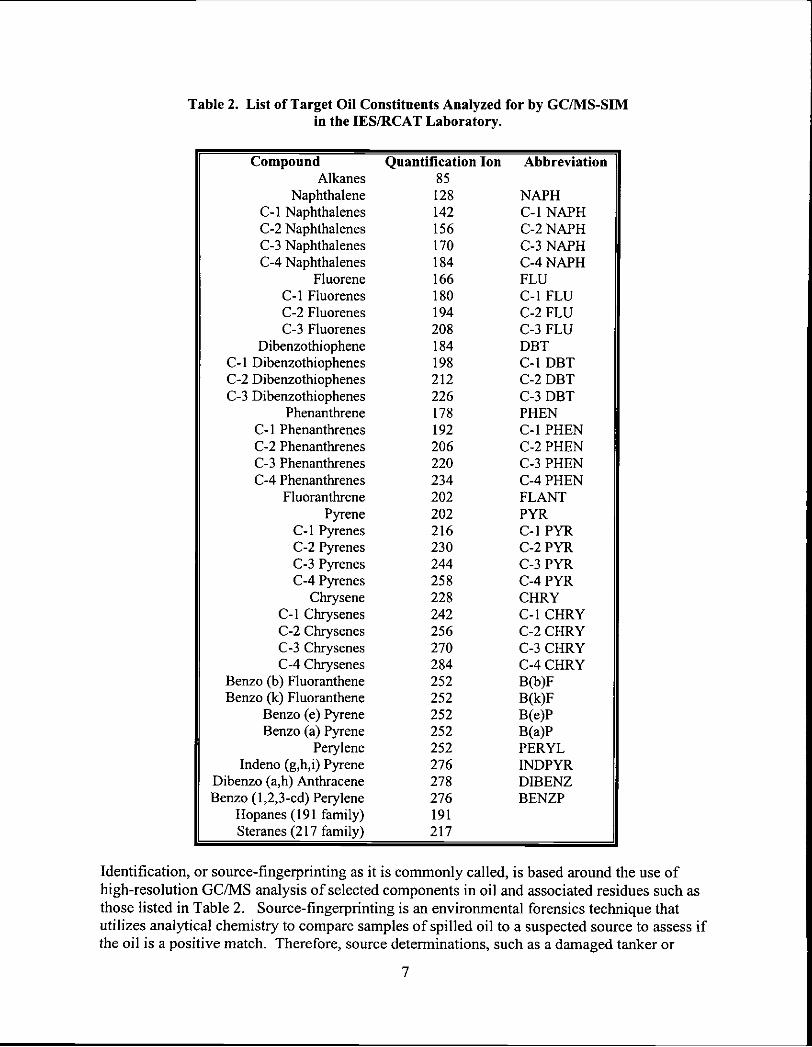
Table 2. List of Target Oil Constituents Analyzed for by GCIMS-SIMin the !ESIRCAT Laboratory.

Compound Quantification Ion AbbreviationAlkanes 85

Naphthalene 128 NAPHC-i Naphthaienes 142 C-i NAPHC-2 Naphthalenes 156 C-2 NAPHC-3 Naphthalenes 170 C-3 NAPHC-4 Naphthalenes 184 C-4 NAPH

Fluorene 166 FLUC-i Fluorenes 180 C-i FLUC-2 Fluorenes 194 C-2 FLUC-3 Fluorenes 208 C-3 FLU

Dibenzothiophene 184 DBTC-i Dibenzothiophenes 198 c-I DBTC-2 Dibenzothiophenes 212 C-2 DBTC-3 Dibenzothiophenes 226 C-3 DBT

Phenanthrene 178 PHENc-i Phenanthrenes 192 c-i PHENC-2 Phenanthrenes 206 C-2 PHENC-3 Phenanthrenes 220 C-3 PHENC-4 Phenanthrenes 234 C-4 PHEN

Fluoranthrene 202 FLANTPyrene 202 PYR

C-i Pyrenes 216 c-I PYRC-2 Pyrenes 230 C-2 PYRC-3 Pyrenes 244 C-3 PYRC-4 Pyrenes 258 C-4 PYR

Chrysene 228 CHRYc-i Chrsenes 242 c-i CHRYc-2 Chs 256 C-2 CHRYC-3 Chsenes 270 C-3 CHRYc-4 ch 284 C-4 CHRY

Benzo (b) Fiuoranthene 252 B(b)FBenzo (k) Fluoranthene 252 B(k)F

Benzo (e) Pyrene 252 B(e)PBenzo (a) Pyrene 252 B(a)P

Perylene 252 PERYLIndeno (g,h,i) Pyrene 276 INDPYR

Dibenzo (a,h) Anthracene 278 DIBENZBenzo (i,2,3-cd) Perylene 276 BENZP

Hopanes (i9i family) 191Steranes (217 family) 217

Identification, or source-fingerprinting as it is commoniy called, is based around the use ofhigh-resolution GC/MS anaiysis of selected components in oil and associated residues such asthose listed in Tabie 2. Source-fingerprinting is an environmentai forensics technique thatutilizes analytical chemistry to compare samples of spilled oil to a suspected source to assess ifthe oil is a positive match. Therefore, source determinations, such as a damaged tanker or

7

deliberate ocean dumping, can be derived. The results of oil fingerprinting are similar to otherforensic analyses (i.e. blood typing) in that oil-fingerprinting techniques provide strongerevidence to prove that a sample is a nonmatch to a suspect source rather than prove, withoutquestion, a positive match. Since oil is a very complex mixture of compounds that cannot becompletely resolved by gas chromatography, a highly selective detector such as a massspectrometer used in conjunction with a high-resolution chemical separation system, the GC,discrimination of specific target compounds from the bulk oil can be achieved. The targetpolycyclic aromatic hydrocarbons (PARs) listed in Table 2 represent less than 5% of the bulkoil composition by weight, and many of the target analytes are present at the low part permillion (ppm) levels in whole or bulk oil. This list of PAHs is highly useful in differentiatingcrude petroleum from byproducts of fuel combustion. This is possible because incompletecombustion of fuels produces PARs that are characterized by 3,4, and 5 ring aromaticcompounds with few substituted alkyl homologues. For example, fluoranthene, chrysene andbenzopyrenes are more common in combustion-sourced pollution than oil pollution.

Quantification of oil and oily residues can be obtained from several different methods. Oil andoil residue concentrations can be directly measured as "total petroleum hydrocarbons" usingappropriate analytical and instrumental (gas chromatograph coupled with a flame ionizationdetector, or GC/FID) methods. However, due to the heterogeneous distribution of oil inaqueous systems and the non-selective properties of the detector, this method requiresextensive replication before statistically valid results can be achieved. Alternately, oilquantities can be inferred by examining the distribution of selected hydrocarbon componentsremaining in oily residues or tarballs found in the environment. This method is based on thefact that not all components in oil are readily degraded by natural weathering processes.Therefore, if the quantities of hydrocarbons that remain are compared to the quantity ofundegraded components, the percent of residual oil remaining after environmental weatheringcan be estimated. Comparing selected hydrocarbon components to the undegraded componentsis known as biomarker normalization. Biomarker normalization shows great promise as a toolfor both identifying spilled oil and quantifying environmental residues. It is not a perfect tooland can, in contaminated systems, overestimate the actual percent degradation. One objectiveof this research is to extend and further validate the use of biomarker normalization byincorporating certain calculated fingerprint indexes that are not subject to day-to-day variancesin an analytical laboratory.

Self-Normalizing Fingerprint Indexes

Since biomarker compounds are more resistant to enviromnental weathering processes,compared to most other oil compounds, they can be utilized as conserved reference compoundsagainst which the loss of less stable oil components can be quantitatively estimated bycalculating certain ratios. These ratios may be useful in differentiating unknown spill samplesfrom a suspected source. Furthermore, the distributions of oil biomarkers is unique fordifferent types and blends of petroleum products and represent an oil-specific fingerprint towhich distinct oil samples can be correlated. Match/nonmatch determinations can be achievedqualitatively through visual comparison of ion chromatogram patterns, and quantitatively fromcalculating the ratio of one biomarker to another. Ratios of certain biomarkers are referred toas self-normalizing fingerprint indexes (SF1) throughout this research. Figures 3 - 8 display

8

the peaks chosen from the biomarker ion chromatograms for calculating the SF1. SF1 arecalculated by using the ratio of different peaks within the same isomer having similar retentiontimes and identical mass to charge ratios. Choosing isomer groups that have similar watersolubilites, vapor pressures, and parent masses will result in potentially useful SF1 andcontribute to the reduction of instrumental variance effects. As instrument conditions changebecause of matrix effects, colunm degradation, sensitivity, or tune degradation, both integersused to calculate the index (assuming they are similar in molecular weight, chemistry andquantitation ion) will be affected by the same relative degree of change; therefore, the index orratio of the two integers, should remain constant. After a corrected base line value and peakheights have been determined, the SF1 are calculated by dividing peak a by peak b (labeled ineach figure).

SF1 are a quantitative teclmique capable of reducing the potential for false-positive results andis not subject to most day-to-day laboratory variances. Goals of the SF1 approach are to reduceinvestigator bias through the use of improved quantitative fingerprint techniques; and allowinvestigators to distinguish subtle differences in actual spill samples that can be easily missedby standard qualitative approaches.

In 1978 Overton and colleagues verified the application of alkyl aromatic ratios in theinvestigation of the fire and oil spill at the West Hackberry, Louisiana, Strategic PetroleumReserve Complex (Overton et al. 1981). They found that the ratio of sulfur containing alkyl-dibenzothiophenes to alkyl-phenanthrenes was distinctly different between the spill oil, anArabian light, and the South Louisiana crude oil (domestically produced and the principalsource of chronic or periodic release in the study area). MatcWnonmatch determinations werederived primarily from qualitative (i.e. visual) comparisons of the chromatographic profiles ofspecific aromatic hydrocarbons and petroleum biomarker compounds such as the steranes andhopanes, as well as indexes derived from specific compound ratios and simple plots.

Visual comparisons of chromatographic fingerprints provide very significant information asopposed to comparison of a few indexes. Visual comparison of a series of analyzed samplesand their corresponding ion fingerprints can easily distinguish one type of oil from anotherbased on the pattern or fingerprint and the ratios of the different constituents within the ionbeing analyzed. Visual match/nonmatch determinations are often criticized as being highlysubjective and potentially biased by the interpreter. However, refined analytical skills,knowledge of oil chemistry, and experience reduce bias and provide a very efficient means fordistinguishing qualitative differences between the fingerprints being compared and can providefurther direction of analysis.

Project Goals

The overall objective of this research was to develop more accurate methods to identify andquantify spilled oil in the environment. Biomarker normalization and self-normalizingfingerprint indexes show great promise as a tool for both identifying spilled oil and quantifyingenvironmental residues. Research performed by IES/RCAT will refine the use of biomarkerscommonly analyzed in our laboratory as tools for oil spill identification and assessment; verify

9

Figure 3. Extracted ion chromatogram (m/e 85) indicatingC-l7JPristane and C-l8lPhytane Sn.

Figure 4. Extracted ion chromatogram (nile 226) indicatingC-3 DBT (a/b) SF!.

10

1lo

1

1x-

75

lOtW

3j.

& (C-Ill-

aEkfl

(C11)

PI1IM)

M 27O ItO ,.fto 2550 d IilSO 1000 XIO 3OO aigo noo ,Ao ,óo

law

law

I IO

:

':

I'

oO aIO

III

aTI OZlOO

II IilIO fllo 'ZO

Figure 5. Extracted ion chromatogram (nile 220) indicatingC-3 Then (a/b) SF1.

Figure 6. Extracted ion chromatogram (nile 216) indicatingC-i Pyr (a/b) Sn.

11

1499

03000

In.

11000

1990

0000

0000

0000

'99

::

00 00 51550 rasot EAD

K

Th0I-4 35.00 34.00 34 3140 34S0 3000 3010 17.00 '744 3440 1IO0 0900 40-00 I0I 4100 414' 4109 4j0I

-Q

000

000

at.

100

199

00 fl109 QISJO*OflJtt D

T40Q 345I fl09 1100 09 360 Zl00 1109 hf00 300 a 000 d09 40.00 4l 410 43135

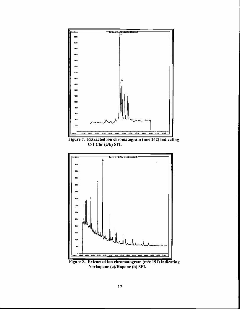
Figure 7. Extracted ion chromatogram (Se 242) indicatingC-i Chr (a/b) Sn.

Figure 8. Extracted ion chromatogram (Se 191) indicatingNorhopane (a)IHopane (b) SF1.

12

24LW

kn24LOO nujobm,ot EOC2Ø&D

1.. 4100 42.00 4120 4200 42.10 4420 44:60 4260 4l70 45.00 4&l0 47.00 47.00

1W

6000

6020

0000

Lx.

3500

Ox.

2000

lx.

Ox.

b.

- Ill 04054006. 451.60&fl

4400 4620 00 6020 64.00 66.00 6620 10.00 6020 64.00 ass w 75.00 7220 7400

this method as compared to the use of other conventional ratio and TPH technologies; andapply this technique to a tarball and oil residue survey along Louisiana's coastline. IES/RCATwill utilize its cache of several collected and preserved reference oils commonly transported inU.S. waters including coastal Louisiana and a few internationally documented sites. Theresearch originally was broken down into eight different research goals, or "tasks" that weredivided into one of four categories: preliminary stages (i.e. literature search and instrumentmethodology); water degradation of one oil in nine natural waters; bioaccumulation ofbiomarker compounds in clams and mussels; and classification and identification of tarballsusing SF1.

Preliminary Stages

The literature search established the foundation for oil biomarkers, past and present, which canbe compared to the oil biomarkers utilized by IES/RCAT. A comprehensive literature reviewof the environmental, petroleum industry, and geological journals was conducted. Informationgained from the literature survey included the identification of various biomarkers and profilesof biomarkers previously determined in petroleum reservoirs from around the world. Keywords utilized during the literature search are given in Table 3.

Table 3. List of Keywords Utilized in the Literature Search.

Assessment OilBiodegradation PAilsBiomarker PersistenceCrude Oil PetroleumFate PollutionFingerprinting Salt MarshFuel Oil SpillHydrocarbon WeatheringOcean

Two previously compiled bib iographies provided additional references and were beneficial inthe initial literature search. The citations for these two bibliographies are:

Light, Melvin and Joseph Lanier. 1978. Biological effects of oil pollution: acomprehensive bibliography with abstracts. US Coast Guard Research andDevelopment Center Report No. CG-D-75-78: 647 pp.

GESAMP (IMO, FAO, UNESCO, WMO, IAEA, UN, UNEP Joint Group ofExperts on the Scientific Aspects of Marine Pollution). 1993. Impact of oiland related chemicals on the marine environment. Rep Stud. GESAMP (50):180 pp.

The literature survey resulted in 180 pertinent articles out of over 300 titles acquired andreviewed. The 180 relevant articles appear in the Appendix titled Biomarkers of PetroleumProducts in the Marine Environment: A Bibliography.

13

The instrument methodology involved the development of an improved GCIMS analyticalmethod that included newly identified biomarker families in addition to those compoundscurrently used for oil spill response. Accomplishment of this stage involved determinationsfrom the literature review and data generated from all the other experiments.

Laboratory-Simulated Weathering and Degradation Study

The water degradation experiment was initially intended to assess compositional changes in sixselected oils due to weathering with respect to biomarker normalization and compositionalchanges within the laboratory. In evaluating the effectiveness of this task in conjunction withpast experience with oils weathered in the environment, it was realized that the major alteringfactor is not the oil compositions that can be identified, but the different types of changes due toenvironmental factors. One significant factor for oil released on water is the ability of thenatural microbial communities within the water to affect the oil composition. Therefore, thewater degradation experimental design was altered to evaluate the changes in the compositionof one oil, a South Louisiana Crude, after exposure to nine natural waters collected across thecountry. Water samples were collected from the coast of Alaska, Hawaii, Florida, Louisiana,California, and from inland waters of the Mississippi River. By evaluating the degradationchanges that occur to the oil when exposed to 28-days of laboratory simulated weathering, inaddition to a simulated nutrient influx and no nutrient inputs, environmental alterations of anoil can be projected, and ultimately affect the emphasis of this research.

In order to determine whether significantly different bacterial communities were present in thevarious waters, nutrient substrate uptake was analyzed with BiologTM microplates. The 96-wellBiologTM microplate contained a variety of carbon and nitrogen sources, as well as a redox dyethat records increases in metabolic rate (Bochner 1989). After the microplate is inoculated withthe bacterial isolate it is incubated, usually for 24 hours. The patterns of positive and negativeresponses are input into a computer through a microplate density reader and the databasescanned for the best statistical match of the substrate utilization profile. Although initiallyutilized for identification of bacterial isolates, the BiologTM system, with some modifications tothe procedure, has been demonstrated to be a reproducible measurement of substrate utilizationby whole bacterial communities and very useful in distinguishing among different communities(Garland and Mills, 1991; Haaek et al., 1995; Wunsche et al. 1995). The results of theBiologTM microplates were used for characterizing the nutrient substrate utilization patterns ofthe microbial communities in each of the water samples.

The final objective of the water degradation experiment was to examine the changes in SF1 forone type of oil pre- and post- weathering. Completion of this task relied upon the SF1generated from pre- and post-weathered Eugene Island Crude (EIC) reference oil utilized in the28-day laboratory simulated weathering step of the water degradation experiment. Statisticalanalysis was performed to determine the stability of the oil biomarkers present in the EIC afterthe 28-days of weathering, along with nutrient or no nutrient additions, and exposure to naturalmicroorganism populations in the different waters tested.

14

Bioaccumulation

The objective of the bioaccumulation experiment was to examine biomarker up-take in bivalvesexposed to oil of known biomarker composition from samples collected recently from PrinceWilliam Sound, Alaska and impacted by the TN Exxon Valdez. Theoretically, biomarkers arenot significantly altered by microbial degradation; hence, there is a possibility that these lipidsoluble materials will accumulate in marine organisms and could be used as an indicator ofpossible exposure during oil spills. The results of this task will establish a time frame in whichbiomarker compounds may be detected in bivalves since the samples were collected ten yearsafter the TN Exxon Valdez incident.

Classification and Identification of Tarballs

The methods of biomarker normalization developed throughout this research were used toanalyze "unknown" environmental samples collected from three areas previously sampled thataccumulated tarballs as documented in the 1993 report titled Characterization of ChronicSources and Impacts of Tar Along the Louisiana Coast by Henry et al. The results of theclassification and identification of the 1998 tarballs further extended the use of the SF1 asbiomarker normalization tools to identif' and estimate relative environmental oil residues. Asemi-quantitative approach for identiing different oil sources based on pattern matches of the(iC/MS fmgerprints and calculated self-normalizing fingerprint indexes were the final resultsof this task.

An initial step in the classification and identification of tarballs included the analysis of theeight biomarker compounds chosen in fourteen unweathered reference oils (two of which weredaily reference oils). The reference oil analysis was performed prior to the analysis of thetarballs collected in 1998. The reference oils were obtained from the IES/RCAT oil library andwere categorized into three groups: crude oils; fuel oils; and other oils (i.e. motor oil).Detailed (iC/MS analysis was performed on these samples and data analysis included thecalculation of the SF1. The results of this task included an attempt to correlate the oils in eachof the categories, and/or support the use of the SF1 for the biomarkers chosen to aid in sourcedetermination since the quantities of biomarkers are different for each type of oil. The SF1 datafrom the reference oils was also utilized to calculate target source areas on double SF1scatterplots containing samples collected during 1992 and 1998, and 1998 alone.

A total of 88 new tarballs were collected in 1998. All 88 of the tarballs were characterizedmorphologically, and 70 tarballs were extracted and analyzed by GC/MS. After the tarballswere analyzed, the SF1 were calculated and a comparison between the SF1 from three sitespreviously sampled in 1992 to the SF1 calculated from the 1998 tarballs from the same threesites was performed. Double SF1 scatterplots were produced for the 1992 and 1998 tarballs,and the 1998 tarballs only. The overall objective of the classification and identification oftarballs was to determine whether or not the SF1 and double index scatterplots used byIES/RCAT are suitable for oil and/or source identification purposes.

15

METHODOLOGY

General Laboratory Methodology

Established good laboratory procedures were utilized throughout the course of the research.All of the sample preparation, experimentation, extraction, and analytical analyses wereconducted at the Institute for Environmental Studies (IES) at Louisiana State University.Samples collected in the field were brought back to the IES/RCAT laboratory to be logged inand given an identification number. The samples were properly stored until time of preparationand extraction.

Quality assurance and quality control was assured through a five-point calibration curve fortarget analytes and internal standards that demonstrated the linear range of the analysis. Afterlinearity of the five-point calibration curve was established, a reference oil (North Slope Crude)and a continuing calibration standard containing naphthalene-d8, anthracene-d10, chrysene-d12, and perylene-d12 was injected every day prior to any sample analysis to verif'instrumental performance.

GC/MS Methodology

Two different Hewlett-Packard 5890 Series GCs coupled with a HP S97lSeries Mass SelectiveDetector were used for all instrumental analyses. Both instruments were equipped with 30meter (m) by 0.250 millimeter (mm) capillary columns with a DB-5 stationary phase and a 0.25micron inner diameter. The GCs were operated in temperature program mode with an initialcolunm temperature of 55°C held for 3 minutes and then increased to 280°C at a rate of 5°C/minute. A final temperature of 300°C was achieved at a rate of 0.5°C/mm and held for 15minutes. The injection temperature was set to 270°C and only high-temperature, low thermalbleed septa were used. The GCIMS interface was maintained at 280°C. Helium gas was usedas the mobile phase. The column head pressure was 13 psi and the flow rate was 1.31milliliters (mL)/min.

The MS was operated in Selected Ion Monitoring (SIM) mode to maximize the detection of thetarget crude oil compounds. The instrument was operated such that the selected ions for eachacquisition window were scanned at a rate greater that 1.5 scans/sec. At the start of an analysisperiod, the MS was tuned to perfluorotributylamine (PFTBA). Nineteen groups with differingscan start times were established and Table 4 provides detailed information for these 19 groups.

Sample introduction into the instruments for the water degradation experiment and the tarballanalysis were achieved by manual injection. Sample introduction for the bioaccumulationstudy was by a HP 6890 Series Auto Injector. One microliter (1iL) of each sample extract wasinjected. Both injectors were operated in splitless mode. FIP Chemstation software was usedfor control, data acquisition and data analysis.

16

Calculation of SF1

All SF1 were calculated from peak height except the C-3 DBT area/C-3 Phen area SF1 that wasdetermined by the division of the area sums (area under each homologues series). Peak heightwas chosen over an area integration method for most of the indexes since the peaks used in thecalculation axe generally not baseline resolved. All peak height determinations were calculatedmanually, corrected for baseline value, and entered into a Microsoft Excel spreadsheet. Referto Figures 3-8 for the peaks chosen from the biomarker ion chromatograms used in thecalculation of the SF1 adapted by IESJRCAT. After a corrected baseline value and peak heightshave been determined, the SF! were calculated by dividing peak a by peak b.

Visual Matching

Comparison of extracted ion chromatographic profiles for the indexes listed in Table 1 wereconducted to determine if any of the samples appear to be related. This process compares therelative composition and extent of weathering for each sample analyzed, providing a detailedinterpretation of the alkylated aromatic hydrocarbon series, sterane, and biomarker distributionpatterns.

The visual method of qualitatively comparing each sample to every other sample is generallyreferred to as the "standard method" and is labor intensive. By this process all the GCIMS datais printed to create a hard copy, sorted by extracted ions and stacked in a pile. Each sample in asingle ion group is compared to the other samples with the same ion to determine if each is amatch or nonmatch. Nonmatch samples form a new pile until every chromatogram has been

Table 4. SIM Ion Grouping for Target Crude Oil Compounds.

17

GroupID

Scan Start Time(minutes)

Ions in Group

1 04.50 82;85;128;136;142;152; 156;166;172; 1802 19.20 85;142;152; 154;156;164;166;l70;172;180;1843 25.00 85;165;166;170;176;178; 179;180;184; 1884 29.00 85;165;178;18O;184;188;192;194;198;2125 30.00 85; 178; 182; 194;208;230;5006 32.00 85; 179; 191;! 92; 194; 1 98;208;212;226;5007 33.00 85; 100; 192; 198;206;208;2!2; 245;260;5008 34.00 85; 101; 1 98;202;206;208;212;226;2609 35.00 85;202;205;206;208;212;2l6;220;226;24510 37.00 85;205;206;216;220;226;234;244;245;50011 39.00 85;205;216;22O;228;230;234;240;244;24812 42.00 85;228;230;234;240;242;244;248;258;50013 44.00 85;230;240;242;244;248;256;258;262;270;27614 46.50 85; 191;252;256;258;262;270;276;28415 47.00 85; 191 ;2 17;252;256;262;270;276;28416 48.00 85; 191 ;2 17;252;256;264;270;276;28417 49.00 85; 191 ;2 l7;252;264;270;276;284;50018 52.00 85; 191 ;21 7;252;253;270;276;278;28419 54.00 85; 191 ;200;2 17;276;278;284;500

compared. The result is generally dozens of small piles of the one ion being compared witheach pile signif5ñng a different source or exhibiting significantly different weathering patterns.The piles are then given an alphanumeric identification.

Laboratory-Simulated Weathering and Degradation Study

The oil used in this experiment was Eugene Island Crude, a type of South Louisiana crude oil.Two, one-liter water samples collected from areas outside of Louisiana included: CoronodoBeach, California; Jax Beach, Florida; and Kilua Beach, Hawaii. Water samples collectedwithin Louisiana included: Holly Beach; water from Lake Charles; Mississippi river watercollected in Port Allen; Price Lake in Rockefeller Refuge; Sabine Lake; and LSU UniversityLakes. Two control waters were also used. One was just deionized water and the other was a32 part per thousand (ppT) Instant Ocean solution. Properties such as salinity, pH, andtemperature were measured in the field. The water samples were brought back to theIES/RCAT laboratory where they were logged in, subsampled and stored at 1°C (34°F) untilthe experiment began

Two, 250mL Erlenmeyer flasks were filled with lOOmL of water from each site. The flaskswere placed on a digital scale (one at a time) and the scale was then tared to zero. A disposable9-inch soda glass pipette was used to add 0 50g of Eugene Island Crude oil to the water. Thefirst flask containing the water and the oil was removed and covered with sterile gauze securedby a rubber band. After the oil was added to the water in the second flask, it was removed andlmL of nutrient mixture was added. The nutrient mixture contained 5g of potassium phosphate(mono), 2.5g of potassium phosphate (dibasic), 2.5g of magnesium sulfate, 5.Og of ammoniumnitrate, and 2.5g of yeast extract in 100 mL of deionized water. The second flask was alsocovered with sterile gauze secured by a rubber band. These steps were repeated twice for atotal of three samples without nutrients and three samples with nutrients for most of the watersamples.

The samples were placed on orbital shakers in two different rooms with two differenttemperatures. The water samples with cooler temperatures at collection were placed on theorbital shaker in the room with an average temp of 23.6°C (74.5°F), and the waters withwarmer temperatures at collection were placed in a room with an average temperature of27.7°C (8 1.9°F). The rotations per minute (rpm) of the two orbital shakers was set to 100 ± 10rpm. The flasks remained on the orbital shaker for 28-days. On the 14th day of the experiment,an additional lmL of nutrients was added to all the flasks originally containing nutrients. Thiswas the only time the orbital shakers were stopped during the course of the experiment.

After 28-days, all the flasks were removed from the shakers to be extracted. Four samples,selected at random from all of the flasks, were poured into 500m1 separatory funnels. The250mL flasks were rinsed with lOmL of dichloromethane (DCM), which was then poured intothe corresponding separatory funnel. This step was repeated two more times for a total of threerinses and 3OmL of DCM Each separatory funnel was inverted and vented several times andallowed to stand for 10 to 30 minutes depending on emulsification. Extent and color of theemulsification for each sample was recorded. A glass funnel with glass wool and anhydroussodium sulfate (Na2SO4) was placed on top of a 4OmL VOA vial and set under each separatory

18

funnel. The Na2504 was moistened with DCM before removal of the 13CM fraction of theextraction in the separatory funnel. DCM was used to rinse the Na2SO4 after removal of theorganic DCM fraction and to reach a final volume of 4OmL for each extract.

After the first set of four extractions was completed, all the equipment utilized was washed andsolvent rinsed prior to the next four extractions. All extracts were capped and stored at 1°C(34°F) until GC/MS analysis.

In addition to this degradation experiment, BiologTM microplate analyses were performed todetermine whether significantly different bacterial communities were present in the variouswaters. For this study, 2mL subsaniples of the water samples collected from the various siteswere frozen at 70°C until analysis. Prior to analysis, lmL aliquots of the samples wereinoculated onto plates containing BUGM agar (Biolog) supplemented with defibrinated sheepsblood to promote abundant growth. The plates were incubated at 37°C ('-424°F) for 72 hours.Cotton swabs were used to transfer bacteria into test tubes containing a sterile saline solution,with salinity adjusted with NaCI to match the salinity of the samples. The saline solution wasinoculated onto the BiologTM microplates using a multipipettor. The plates were incubated for3 days at 37°C ('-424°F), in a modification of a technique used for soil samples (Garland andMills 1991). The yeast extract solution was then inoculated directly onto the BiologTM plates.

Finally, pre- and post-weathered Eugene Island Crude oil samples were analyzed. The pre-weathered oil sample utilized was prepared by adding 0.25 grams of ETC to 10 mL of hexane,and was manually injected everyday prior to analysis of the extracts. The post-weathered ETCsamples were obtained from the extracted waters after 28-days of weathering on the orbitalshaker. SF1 were calculated after HP Chemstation data integration. The stability of thebiomarker SF1 was determined through statistical analysis of each individual SF1.

Bioaccumulation

Because biomarkers are not significantly altered by microbial degradation, there is thepossibility that these lipid soluble materials will accumulate in marine organisms and could beused as an indicator of possible exposure during oil spills. Selected marine bivalves recentlycollected and still exposed to the TN Exxon Valdez oil were analyzed for composition, uptakeand alteration of hydrocarbon components including the biomarker compounds. Biomarkersnormally elute in the biogenic lipids fraction (Fl) during size exclusion chromatographicfractionation. Fl fractions from 6 mussel tissues and 6 clam tissues from different collectionsites in Prince William Sound (PWS), along with a blank and rotary evaporator blank for eachtissue type, were analyzed by the GCIMS-SIM method given previously in the methodology.

An IES/RCAT scientist collected the tissue samples during the National Oceanographic andAtmospheric Administration's (NOAA) summer monitoring cruise of PWS in 1999. Thesamples arrive at the IES/RCAT laboratory frozen and in ice chests. They are logged in, givena LSU ID#, and stored in a freezer until they are removed to be cleaned. The external shell andtissue of all bivalves in each sample were rinsed with deionized water to remove any particlesor extraneous material. The animals were removed from their shells and placed into a

19

precleaned jar. A Teckmar TissuemizerTM was used to homogenize each sample. Allhomogenized samples were stored in a freezer until extraction.

Approximately 5g of the homogenized tissue was removed from the sample and placed into acleaned, 5OmL beaker and spiked with surrogate standards. Between 15 to 25g of Na2SO4 wasadded to the tissues depending upon the amount of water within the tissues or until a pasteconsistency was obtained. The extraction solvent, DCM, was added in 35mL aliquots to thesample. The samples were then placed in a sonicator for 15 minutes. The solvent extract wasthen filtered through additional Na2SO4 and glass wool into a round bottom flask. Theextraction procedure was carried out a total of three times for each sample.

To concentrate the solvent extract, the sample was rotary evaporated to approximately 8mLfinal volume. The concentrated extract was split into 4mL for lipid analysis and 4inL for PAHanalysis. The samples were then fractionated using alumina/silica gel solid phase extraction.The first fraction, or the Fl fraction, is usually composed of lipid compounds in hexane. Afinal Fl fraction volume of 4mL was stored in a vial until concentrated under a gentle stream ofnitrogen to a final volume of 0.lmL A lmL Hamilton Gas tight syringe was used to transferthe 0. lmL sample into a 2mL autosampler vial containing 100 kL wide opening inserts. Tenmicroliters of a 100 jiglmL internal standard were added to each of the samples. The vials werecapped with aluminum/PTFE lined crimp caps.

An HP 6890 Auto Injector was used to inject lj.tL onto the GC column for this task. Afteranalysis, HP Chemstation software was utilized to integrate the compounds listed in Table 2 onpage 7. After integration, the peak areas for each of the samples were transferred into aspreadsheet where the concentrations, in parts per billion, were calculated.

Class Wcation and Iden4flcation of Tarballs

Fourteen reference oil samples were prepared by adding 0.25 grams (g) of oil into lOmL ofhexane. Oils selected from the IES/RCAT oil library included: Arabian Light Crude; BasrahCrude; Bunker C; Diesel No. 2 Fuel Oil; Eugene Island Crude; Hondo; ff0 380; LouisianaBlend; Mega Borg Light Crude; North Slope Crude; South Louisiana Crude; 55 Block 126Condensate; Strategic Petroleum Reserve Crude; and Valvoline SAE 30. The North SlopeCrude oil was used to check daily instrument responses. The Eugene Island Crude oil was usedduring the water degradation experiment. One microliter of the oil in hexane was manuallyinjected into the GC/MS. SF1 were calculated as stated previously and entered into aspreadsheet. The SF1 for all the oils were divided into three types of oilS crude; fuel; and other.Statistical analysis was performed to determine, if any, correlation within the three categories.

Tarballs for the 1998 classification and identification field study were collected from three sitesin the southwestern portion of the Louisiana Gulf Coast that were sampled previously in 1992.Nine original sampling locations were designated in 1992 and are given in the report titled:Characterization of Chronic Sources and Impacts of Tar along the Louisiana Coast by C.B.Hemy, P.O. Roberts, and E.B. Overton (1993). Only three of the nine original station locationswere revisited in 1998 (Figure 9). The three stations revisited were: Martin's Beach; HollyBeach; and Rutherford Beach.

20

MARTINS BEACH

RUTHERFORD BEACHOLLY BEACH

92°

at

21

4

91°.. - ;C-

5° MILESI I

I,

0 50 KILOMETERS

-_____ p - Søffl .t W 4??- 300

Figure 9. Sampling locations along the Louisiana coastline for stranded oil andtar survey, 1998.

Each sampling location was subdivided during sampling into backshore and foreshore regions.The backshore region is defined as the area behind the high tide debris line and includes thestorm berm area. The foreshore area included the high tide debris line down to the water'sedge. The differentiation between the foreshore and backshore was intended to distinguishbetween recently deposited oil (i.e. from the last high tide) and oil deposited in the upper beachfrom past storm activities. Tarball collection was performed by systematically walking eachsampling location, collecting all tarballs which were greater than a few millimeters in size, andwrapping each individually in aluminum foil. All samples were stored at ambient temperaturewhile in the field.

For the 1998 survey, a total of 52 tar balls were collected from Martins Beach (47 from theforeshore, one from midshore, four from backshore); 10 tarballs were collected from HollyBeach (eight from the foreshore, two from the backshore); and 26 tarballs were collected fromRutherford beach (25 from the foreshore, one from the midshore). The cumulative tarball totalwas 88, of which 70 were sampled and analyzed. Eighteen samples were not extracted due tothe fact that they were smaller than the cutoff weight established during the morphologicalcharacterization step of analysis; or were pieces of asphalt too hard to sample.

Once the tarballs were brought back to the lab, they were weighed, and visually and physicallycharacterized. Morphological characterizations included: outside/inside color, extraneousmaterials, pliability, and any comments regarding the outside/inside texture. The colorcategories were black, black-red, brown, grey, green, and white. Extraneous materials werevisually estimated as a percentage of organic, sand, and shell. Materials considered as organicmatter were seaweed and other plant material, and occasionally worms. Barnacles on theoutside surface were considered when determining the percent range for shell composition.Pliability was also determined and ranked from 0 to 5 by the extent the tarball would bendwhen manual pressure was applied. A value of 0 represents solid tarballs without anypliability, while 5 indicated stranded tar that is almost fluid at ambient laboratory roomtemperature. A pliability ranking of 3 is representative of tar pieces that can bend without

- 29°89°

breaking. The pliability characteristic can be related to some degree to the residual oil's pour-point and provide insight to the extent of weathering.

Each tarball was cut in half (after being weighed) and any additional comments were noted inregards to the appearance of the interior portion of the sample. Common interior descriptionswere glassy, slightly glassy, shiny, slightly shiny, and dull. These descriptions were used inconjunction with a description of the texture of the tarball interior which included hard,relatively soft, soft, waxy, grainy/gritty, and rocky. All of these observations were qualitativeonly and decided on by the researcher.

A 0.20 to 0.30g core of each tarball was sampled and placed into individual 4OmL VOA vials.The average weight of the samples was 0.22g. Two grams of Na2SO4 were added to all thevials. Ten milliliters of hexane were then added to each vial. The samples were sonicated in acold bath for 15 to 20 minutes. After sonication, the vials were refrigerated at 1°C (34°F) untilGC/MS analysis. After GC/MS analysis, the samples were integrated and the SF1 werecalculated as stated previously in the methodology and entered into a spreadsheet.

Visual classification of the tarballs was based on a source classification scheme established byHenry et al. in the 1993 report Characterization of Chronic Sources and Impacts of Tar alongthe Louisiana Coast. The tarballs for this report were classified into one of nine categories:relatively unweathered, high aromatic; relatively unweathered, high paraffin; relativelyunweathered bimodal wax; weathered, high aromatic; weathered, high paraffin; weathered,bimodal unresolved complex mixture (UCM); weathered, bimodal wax; weathered, bimodalUCM, and wax (trimodal); and unclassifiable.

A slightly modified version of the same source classification was utilized to separate thetarballs collected during the 1998 survey (i.e. high was not used as a descriptive of the type ofoil and only eight categories, instead of nine, were established for the 1998 tarballs). Thecategories for the 1998 tarballs were classified into one of eight categories: relativelyunweathered, aromatic; relatively unweathered, paraffin; relatively unweathered, wax/bimodalwax; weathered, aromatic; weathered, paraffin; weathered, wax/bimodal wax; weathered,UCM; and unclassifiable.

SF1 from the tarballs collected in 1992 were then compared to the SF1 calculated for the tarballscollected in 1998. Data for 27 of the 1992 tarballs was obtained from Appendix II in Henry etal.'s 1993 report. Data for the 1998 samples totaled 69 tarballs. Double index scatterplotswere then generated with the SF1 data from both years. SF1 data from twelve of the fourteenreference oils (excluding North Slope Crude and Eugene Island Crude) were also plotted todetermine, if possible, source of the tarballs andlor if any of the tarballs from both yearsmatched each other. Calculating ±20% of the x-axis SF1 and y-axis SF1 for each reference oilestablished target match zones.

The 1998 tarballs were plotted alone on another set of double SF1 scatterplots with thereference oil target match zones. The tarballs included in the target zones were visuallycompared to the reference oil and/or other tarballs in the zone. Match/nomnatch determinations

22

were then made. Data evaluation also included an extensive visual matching process for theeight biomarker fingerprints.

RESULTS AND DISCUSSION

Laboratory-Simulated Weathering and Degradation Study

The original goal of the water degradation study was to assess compositional changes in sixselected oils due to weathering with respect to biomarker nonnalization and compositionalchanges within the laboratory. However, after some consideration, it was decided that studyingthe ability of microbial communities to naturally degrade oils would be more prudent. Themajor altering factor, in regards to oil degradation in the marine environment, is the effectcaused by the natural microbial communities within the water. This task evaluated the changesin composition of one oil, Eugene Island Crude (EIC), after exposure to nine natural waterscollected across the country and two control waters, after 28-days of weathering.

Two analytical endpoints, percent change in total target aromatic hydrocarbons (TTAH) andthe stability of the SF1, were chosen to assess the biodegradation and biomarker persistence ofthe one oil (EIC) in the nine water samples and the two control waters. The change in TTAH isreflective of bulk oil loss; while the SF1 represent specific classes of biodegradation-resistivehydrocarbons, or biomarkers.

Table S gives the percent reduction in total target aromatic hydrocarbons after the 28-dayweathering period for the nine water sites and Figure 10 shows the sum of TTAH in thesamples with and without nutrients analyzed after 28-days of weathering. Abiotic factors thatmay affect the degradation of the ETC were controlled to some extent; the oil was the same andtemperatures remained relatively constant in both experimental locations. One importantabiotic factor not capable of being replicated in the laboratory study was the effect of tides.Oxygen and nutrients, often the limiting factors in real world situations, were provided to themicrobial communities present in the different waters (i.e. the flasks were covered with sterilegauze and nutrients were provided to half the flasks). Biodegradation potentials of each waterwith additional nutrients were readily apparent in the percent reduction of TTAH.

Table 5. Percent of TTAII Reduction for the Nine Water SamplesAfter 28-Day Weathering Experiment.

23

% Reduction,No Nutrients

% Reduction,With Nutrients

Fresh Water SitesLake Charles, LA 37 87

Port Allen, LA 15 68(Mississippi River water)Rockefeller Refuge, LA 43 88

Sabine Lake, LA 19 49LSU University Lakes, LA 39 93

(Table 5 Continued)

Figure 10. Average TTAH for each site and two controls.

BiologTM microplate analyses were also performed for the nine water sites in order to provide apreliminary characterization of the microbial communities present in the waters and theirability to utilized a variety of carbon sources. The results of the BiologTM microplate analysesindicate that the bacteria in the different water samples had widely varying metaboliccapabilities. For purposes of comparison among samples, carbon sources were groupedaccording to compound type and then the response to compounds within the class averaged.Full responses (indicated by high color development in the well) was given a rating of 100, lowresponse a rating of 50, and no response a rating of 0. Compound classes included (1)polymers, (2) carbohydrates, (3) esters, (4) carboxylic acids, (5) brominated chemicals, (6)amides, (7) amino acids, (8) aromatic chemicals, (9) amines, (10) alcohols, and (11)phosphorylated chemicals. The total number of sources used was also calculated. Figure 11provides the total sources, as calculated from the BiologTM results, used by the indigenousmicroorganisms from each water. The carbon source of interest for correlation to thelaboratory weathering is the aromatic chemicals. Figure 12 displays the percent aromaticchemicals utilized by the indigenous microorganisms present in each of the water samples.

24

% Reduction,No Nutrients

% Reduction,With Nutrients

Salt Water SitesCoronodo Beach, CA 17 76

buy Beach, LA 30 90Jax Beach, FL 0 74

Kilua Beach, HI 0 35

The results of the BiologTM microplates do not correlate well with the TTAH endpoint. Theresults of the 28-day weathering experiment demonstrate that LSU University Lakes water withthe additional nutrients had the highest percent change, 93%, in total target aromatichydrocarbons. This is interpreted as the water from University Lakes and the indigenousmicrobial community present utilized the oil more efficiently than the other waters. The lakesare subjected to chronic, urban runoff that results in a constant flux of nutrients and oxygendemands. The results of the BiologTM microplates show the opposite of this conclusion. LSUUniversity Lakes had a low response in both total source utilization and aromatic chemicalutilization. This could be due to several factors. The aromatic chemicals provided as a carbonsource in the BiologTM microplates consisted of urocanic acid, inosine, uridine and thymidine.The carbon source in the 28-day weathering experiment was a crude oil that was analyzed for40 different petroleum hydrocarbons. The nutrient substrates also differed. BiologTM utilizedBUGM agar supplemented with defibrinated sheep's blood; the 28-day weathering studyutilized a nutrient mixture containing potassium mono-phosphate, potassium dibasic phosphate,magnesium sulfate, ammonium nitrate and yeast extract. Larger samples of water should havebeen taken for the BiologTM analyses to provide a more sufficient sample to be cultured. Only 2mL of water from each collection site was saved for the microplate analysis.

The differences in nutrient substrate and carbon sources available in the natural environmentand in the experimental flasks could have affected the combined metabolic utilization of themicrobial community present in each of the waters tested. As a result, dominant species mayhave been different for the BiologTM and the 28-day weathering experiment. Furthermore,Smalla et al. (1998) found that the relative abundance of populations present in the inoculachanges during incubation of the BiologTM plates, resulting in a dominance of species that arebest able to compete with the substrate concentrations in the microplates and under theconditions of incubation. Both experiments provide information on the microbial populationsas a whole and how they work together to degrade sources of nutrients provided for them.

It appears as though the temperature of the two experimental locations may have had an effecton the degradation potential of the nine water sites. The temperature of each water wasrecorded at the time of collection, along with other physical characteristics such as salinity andpH. When the waters were brought back to the laboratory, they were stored in a refrigeratoruntil sample preparation, at with time the samples were removed. Two different experimentallocations were established to correspond to the approximate collection temperature of the watersamples. One room had an average temperature of 23.3°C (73.9°F) and the other room had anaverage temperature of 27.4°C (81.4°F). The percent reduction in TTAH for the samples in theroom with the warmer average temperature, with one exception, was almost one to three ordersof magnitude higher than the percent reduction in TTAH for the samples in the room with thecooler temperature. The one exception was the water sample from Sabine Lake. Averageambient temperature of the two experimental locations appears to only affect the percent TTAHreduction for the no nutrients. Table 6 contains the physical characteristic data and the percentreduction of TTAH for the nine water samples and is sorted based on the average temperatureof the two rooms.

25

100

90

80

I70

60

50

40

30-

20

10 I0, I, /j%/f,tP # ...0

>,

C,0

Collection Site

'u'.''Figure 11. Total sources utilized by microorganisms from Biolog TM results.

100

90

80

70

60

50

40

30

20

10

0--I..'.., ,.

4M$' \\C; ç>%6 ç4# $ \ 0

C'0

Collection Site

Figure 12. Percent aromatic chemicals utilized by microorganisms from BiologTM results.

26

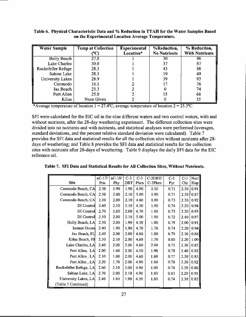
Table 6. Physical Characteristic Data and % Reduction in TTAH for the Water Samples Basedon the Experimental Location Average Temperature.

*Average temperature of location 1 = 27.4°C; average temperature of location 2 = 23.3°C

SF1 were calculated for the ETC oil in the nine different waters and two control waters, with andwithout nutrients, after the 28-day weathering experiment. The different collection sites weredivided into no nutrients and with nutrients, and statistical analyses were performed (averages,standard deviations, and the percent relative standard deviation were calculated). Table 7provides the SF1 data and statistical results for all the collection sites without nutrients after 28-days of weathering; and Table 8 provides the SF1 data and statistical results for the collectionsites with nutrients after 28-days of weathering. Table 9 displays the daily SF1 data for the EICreference oil.

Table 7. SF1 Data and Statistical Results for All Collection Sites, Without Nutrients.

27

Water Sample Temp at Collection(°C)

ExperimentalLocation*

%Reduction,No Nutrients

% Reduction,With Nutrients

Holly Beach 27.8 1 30 90Lake Charles 30.0 1 37 87

Rockefeller Refuge 28.3 1 43 88Sabine Lake 28.3 1 19 49

University Lakes 28.9 1 39 93Coronodo 16.1 2 17 76Jax Beach 23.3 2 0 74Port Allen 25.0 2 15 68

Kilua None Given 2 0 35

SitenC-17!

PñsnC-181

PhyC-3DBT

C-3Phen

C-3DBT!C-3Phen

C-IPyr

C-iChr

Nor!Hop

Coronodo Beach, CA 2.30 1.90 1.90 4.90 1.10 0.71 2.30 0.91Coronodo Beach, CA 2.50 2.00 2.10 5.00 1.90 0.71 2.30 0.87Coronodo Beach, CA 2.30 2.00 2.10 4.60 1.90 0.73 2.30 0.92

DiControl 2.60 2.10 2.10 4.30 1.90 0.74 2.20 0.94DI Control 2.70 1.80 2.00 4.70 1.90 0.75 2.20 0.93DI Control 2.50 2.00 2.10 5.00 1.90 0.72 2.40 0.97

Holly Beach, LA 2.50 2.00 i.90 4.30 1.80 0.79 2.00 0.91Instant Ocean 2.40 1.90 1.90 4.70 1.70 0.74 2.20 0.94JaxBeach,FL 2.40 2.00 2.00 4.80 1.80 0.79 2.30 0.86

Kilau Beach, HI 2.50 2.10 2.00 4.60 1.70 0.80 2.20 1.00

Lake Charles, LA 2.40 2.00 2.00 4.60 2.00 0.75 2.30 0.85

PortAllen, LA 2.00 1.60 2.00 4.50 1.90 0.78 2.40 0.92Port Allen ,LA 2.10 1.60 2.00 4.60 1.80 0.77 2.30 0.85PortAllen,LA 2.20 1.70 2.00 4.90 1.80 0.78 2.30 0.92

Rockefeller Reffige, LA 2.60 2.10 2.00 4.90 1.90 0.76 2.30 0.86Sabine Lake, LA 2.70 2.00 2.10 4.90 1.80 0.83 2.20 0.91

University Lakes, LA 2.40 1.80 1.90 4.50 1.80 0.74 2.30 0.82(Table 7 Continued)

Table 8. SF1 Data and Statistical Results for All The Collection Sites, With Nutrients.

Table 9. SF1 Data and Statistical Results for Daily EIC Reference Oil.

28

nC-17/Pris

nC-18/Phy

C-3DBT

C-3Phen

C-3DBT/C-3Phen

C.1Pyr

C-iChr

Nor!Hop

Average 2.42 1.92 2.01 4.69 1.80 0.76 2.26 0.90Standard Deviation 0.19 0.16 0.07 0.22 0.20 0.03 0.09 0.05

Percent Relative StandardDeviation 8.04 8.50 3.73 4.73 10.94 4.43 4.11 5.22

SitenC-17/

PnisnC-18/

PhyC-3DBT

C-3Phen

C.3DBT/C-3Phen

C-iPyr

C-iChr

NonHop

Coronodo Beach, CA 0.00 0.00 2.20 4.80 1.70 0.69 2.20 0.94

CoronodoBeach,CA 0.00 0.00 2.10 5.10 1.80 0.73 2.20 0.92Coronodo Reach, CA 0.00 0.00 2.20 5.70 1.80 0.00 2.20 0.90

DI Control 0.61 0.00 2.20 4.90 1.80 0.76 2.50 0.89DI ControL 1.80 0.00 2.00 5.10 1.80 0.72 2.30 0.84

DI Control 0.71 0.00 2.20 4.90 1.90 0.74 2.40 0.88

Holly Beach, LA 0.00 0.00 2.10 7.30 2.20 0.00 4.50 0.89

Instant Ocean 0.06 0.04 2.10 5.00 1.80 0.77 2.20 0.91

Jax Beach, FL 0.00 0.00 1.50 6.40 2.00 0.00 3.20 0.90

Jax Beach, FL 0.52 0.20 2.50 4.80 1.90 0.70 2.20 0.91

Jax Beach, FL 0.00 0.00 2.00 6.10 2.00 0.85 4.30 0.92

Kilua Bch, HI 0.11 0.01 2.10 5.20 1.90 0.80 2.40 0.92

Kilua Bch, HI 0.21 0.13 2.20 5.50 1.80 0.84 2.30 1.00

Kilua Bch, HI 0.03 0.03 2.00 4.30 1.80 0.74 2.30 0.87

Lake Charles, LA 0.90 0.15 1.40 8.10 1.70 0.45 3.20 0.86

Port Allen, LA 0.00 0.00 2.00 5.30 1.60 0.65 2.20 0.92

Port Allen, LA 0.00 0.00 2.10 4.40 1.70 0.76 2.40 1.00

Pod Allen, LA 0.00 0.00 2.20 6.10 1.60 0.84 2.56 0.89Rockefeller Refuge, LA 0.00 0.00 1.80 7.80 1.80 0.54 3.20 1.00

Sabine Lake, LA 0.61 0.17 1.90 5.30 1.90 0.73 2.40 0.90University Lakes, LA 0.00 0.00 2.30 6.70 1.50 0.00 2.50 0.88University Lakes, LA 0.37 0.00 2.40 6.20 1.70 0.00 4.40 0.95University Lakes, LA 0.00 0.00 1.90 4.30 1.00 0.00 13.80 0.90

Average 0.26 0.03 2.06 5.62 1.77 0.54 3.21 0.91

Standard Deviation 0.44 0.06 0.25 1.07 0.22 0.34 2.42 0.04Percent Relative

Standard Deviation 170.22 198.96 12.13 18.95 12.69 62.93 75.43 4.64

EIC Ref OilnC-17/

PrisnC-IS!

PhyC-3DBT

C-3Phen

C-3DBT/C-3Phen

C-iPyr

C-iChr

Nor!Hop

Rep 1 2.30 2.00 1.80 4.20 1.80 0.75 2.20 0.90Rep 2 2.40 1.90 1.80 4.10 1.70 0.77 2.00 1.00

Rep 3 2.20 1.90 1.80 4.50 1.80 0.73 3.80 0.97(Table 9 Continued)

The SF1 for the ETC after 28-days of weathering and no nutrients in the nine waters and twocontrols were acceptable based on the percent relative standard deviation (%RSD), whichranged from 4% to 11%. Acceptable data can be defined in many ways and is usually governedby the criteria established in different scientific fields. For the Environmental ProtectionAgency, acceptable data is anything less than or equal to 25% RSD. The SF1 for the daily ETCanalysis had similar results to the weathered EIC. Percent relative standard deviations for thedaily EIC SF1 ranged from 3% to 22%.

The nC-i7fPris and nC-18/Phy SF1 for all the waters with nutrients would not be acceptable touse for accurate determinations of source based on their %RSD, 170% and 199% respectively.However, they should not be entirely overlooked due to the fact that they would provideinformation in regards to the extent of weathering. The C-i Pyr and C-i Chr SF1 were alsounacceptable as shown by their %RSD (63% and 75% respectively).

When each water sampling site was analyzed individually, most of the waters with theadditional nutrients had nC-17/pris and nC-i8/phy SF1 that were either not within acceptabledata limits (%RSD of 25 or less) or no peaks were present in the ion chromatogram to calculatethe SF1 (this would result in an SF1 of 0.00). There were three sites out of nine and twocontrols that contained unacceptable relative standard deviations (>25% RSD) for SF1 otherthan the nC-i7/Pris and nC-l8IPhy. Coronodo beach, no nutrients, had an unacceptable C-3DBT arealC-3 Phen area SF1 (RSD=28%) and an unacceptable C- 1 Pyr SF1 for the sampleswith nutrients (RSD=87%). Jax Beach had unacceptable data for C-i Pyr and C-I Chr SF1 forsamples containing nutrients (RSD=88% and 33% respectively). The third site withunacceptable data was University Lakes with nutrients; %RSD for the C-3 DBT area/C-3 Phenarea SF1 was 26% and the C-1 Chr SF1 was 88%. All of the other individual sites, with andwithout nutrients had SF1 ranging from 0 to 25% RSD. Despite some of the individual sitedata, the water degradation study provides the best evidence of the stability of the biomarkercompounds analyzed (refer again to Tables 7, 8, and 9).

The SF1 that would provide the best information in regards to proving that a sample of spilledoil is a match/nonmatch to a suspect source would be C-3 DBT; C-3 Phen; C-3 DBT arealC-3Phen area; and Nor/Hop (refer to Figures 4, 5, and 8 respectively for fingerprint). Thesecompounds and their calculated SF1 will distinguish one oil type from another, even oils of

29

EIC Ref OilnC-17/

PrisnC-iS!

PhyC-3

DBTC-3Phen

C-3DBT!C-3Phen

C-iPyr

C-IChr

Nor!Hop

Rep4 2.30 1.90 1.90 6.50 1.70 0.85 2.30 0.94

RepS 2.40 2.00 1.90 4.30 1.70 0.84 2.20 0.91

Rep 6 2.40 1.80 1.90 4.30 1.70 0.78 2.30 0.94

Rep 7 2.30 1.90 2.00 7.00 1.70 0.76 2.20 0.91

RepS 2.40 1.90 2.00 4.80 1.80 0.75 2.10 0.93Rep 9 2.50 2.00 1.90 4.10 1.70 0.79 2.30 0.97

Rep 10 2.30 1.90 2.00 4.60 1.90 0.81 2.10 0.93Average 2.35 1.92 1.90 4.84 1.75 0.78 2.35 0.94

Standard Deviation 0.08 0.06 0.08 1.04 0.07 0.04 0.52 0.03Percent Relative Standard

Deviation 3.62 3.29 4.30 21.43 4.04 5.07 22.09 3.36

similar geographical origin, when other target biomarkers and analytes are lost. Aninvestigator using these four SF1 will have the ability to distinguish subtle differences in actualspill samples that can be easily missed by standard qualitative approaches (i.e. visualmatching). The C-3 DBT, C-3 Phen, C-3 DBT area/C-3 Phen area, and Nor/Hop SF1, whenused in conjunction with double SF1 scatterplots with a 20% target zone for the reference oiland visual comparisons, will further assure the investigator in determining matchlnonmatch ofthe unknown sample to the reference oil and other unknown samples. The remaining SF1, (nC-17/Pris; nC-18/Phy; C-i Pyr; and C-i Chr) appear to be greatly affected by weathering (%RSDwere greater than 25 for the ETC after 28-days of weathering). Regardless of the fact that thesefour SF1 were not within acceptable statistical ranges, visual examination of the correspondingfingerprint will still aid the investigator in match!nonmatch determinations.

Bioaccumulation

Up-take of biomarkers and, in general PAHs, were examined in bivalves exposed to oil fromthe TAT Exxon Valdez. The samples were collected in 1999 from Prince William Sound,Alaska, 10 years after the TN Exxon Valdez spill. Since biomarkers are not usually altered bymicrobial degradation, there is a possibility that these lipid soluble materials will accumulate inmarine organisms and could be used as an indicator of possible exposure during oil spills.

Since biomarkers normally elute with biogenic lipids during chromatographic fractionation (Flfraction), random samples of seven Fl mussel tissues and six Fi clam tissues were analyzed byGC/MS. Figure 13 is a histogram of the mussel tissue analysis. One mussel sample (LSU ID#N9201-22) included in the Fl fraction analysis was taken from a dock that undergoes chronicpollution from boats. This sample had the highest concentration of both total target aromatichydrocarbons (TTAH; synonymous with total polycyclic aromatic hydrocarbons or PAH5) andbiomarker compounds; however, a baseline concentration of biomarker compounds has notbeen established for biological samples from the beginning of the TN Exxon Valdez spill.

Figure 14 is a histogram of the clam tissue analysis. Both histograms have the TTAH andbiomarker concentrations given in parts per billion (ppb).

The Fl analysis provides important information about the uptake and utilization of petroleumhydrocarbons by filter feeding organisms after a duration of time that would be difficult toperform in a laboratory based experiment. Overall, the biomarker concentrations for bothtissue types were low. The PAH and biomarker concentrations in the Fl fractions from theclam tissues were lower than the mussel. Detection limits of the GC/MS utilized for theanalysis was 0.01 ppb. The low levels of both PAHs and biomarkers can be viewed in one oftwo ways: the mussel and clam tissues almost have non-detectable quantities of petroleumhydrocarbons; or biomarker compounds are not at detectable concentrations in biologicalsamples 10 years after exposure to oil. The concentrations of PAHs in the tissue samples fromPrince William Sound have been relatively low the past few years.

Two factors that may explain the low levels are the metabolic capabilities of the mussels andclams, and the age of the population sampled in 1999. Generally, biomarkers are resistant tobiodegradation, which implies bacterial degradation and not enzymatic transformation. Thelife span of the mussel and clam organisms themselves is another factor. The population

30

sampled in 1999 may have been either newly established populations, therefore exposed tolower concentrations of oil to begin with; or the population was well established and was ableto readily metabolize the petroleum compounds. Unfortunately, biomarker analysis or SF1were not calculated for any of the samples from previous years, and as a result, a baselinebiomarker concentration was not established. In regards to the literature review concerningbiological tissue samples, the focus was on bioavailability of PAMs compounds in the marineenvironment and not biotransformation.

Figure 13. Total polycyclic aromatic hydrocarbons (PAils) and biomarkerconcentrations in Fl fractions from 1999 PWS mussel tissues.

2

1.8

1.6

= IAC.3' 1.2

0.8

0.6.

o 0.4

0.2

4 #1Clam Sample ID#

o Biomarkers

flAH

Figure 14. Total polycyclic aromatic hydrocarbons (PARs) and biomarkerconcentrations in Fl fractions from 1999 PWS clam tissues.

31

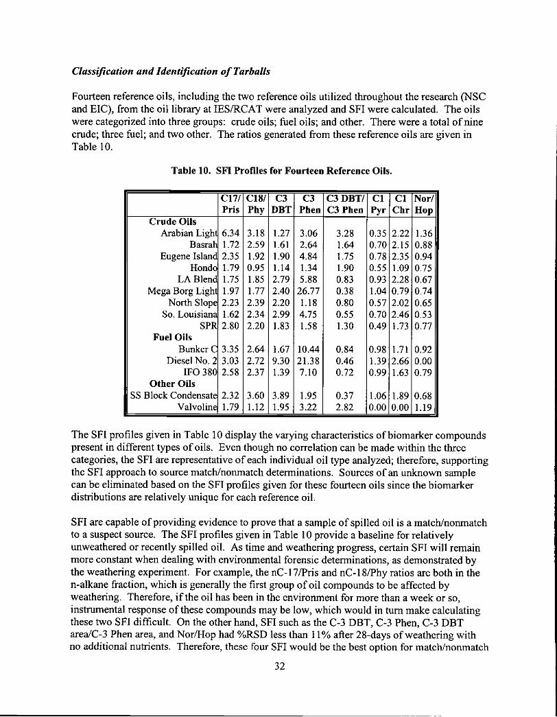
Class jfication and Identification of Tarballs

Fourteen reference oils, including the two reference oils utilized throughout the research (NSCand EIC), from the oil library at IES/RCAT were analyzed and SF1 were calculated. The oilswere categorized into three groups: crude oils; fuel oils; and other. There were a total of ninecrude; three fuel; and two other. The ratios generated from these reference oils are given inTable 10.

Table 10. SF1 Profiles for Fourteen Reference Oils.

The SF1 profiles given in Table 10 display the varying characteristics of biomarker compoundspresent in different types of oils. Even though no correlation can be made within the threecategories, the SF1 are representative of each individual oil type analyzed; therefore, supportingthe SF1 approach to source matchlnonmatch determinations. Sources of an unknown samplecan be eliminated based on the SF1 profiles given for these fourteen oils since the biomarkerdistributions are relatively unique for each reference oil.

SF1 are capable of providing evidence to prove that a sample of spilled oil is a matchlnomnatchto a suspect source. The SF1 profiles given in Table 10 provide a baseline for relativelyunweathered or recently spilled oil. As time and weathering progress, certain SF1 will remainmore constant when dealing with environmental forensic determinations, as demonstrated bythe weathering experiment. For example, the nC-l7IPris and nC-18/Phy ratios are both in then-alkane fraction, which is generally the first group of oil compounds to be affected byweathering. Therefore, if the oil has been in the environment for more than a week or so,instrumental response of these compounds may be low, which would in tum make calculatingthese two SF1 difficult. On the other hand, SF1 such as the C-3 DBT, C-3 Phen, C-3 DBTarealC-3 Phen area, and Nor/Hop had %RSD less than 11% after 28-days of weathering withno additional nutrients. Therefore, these four SF1 would be the best option for match/nonmatch

32

C171Pris

C181Phy

C3DBT

C3Phen

C3DBT/C3 Then

ClPyr

ClChr

Nor!Hop

Crude OilsArabian Ligh 6.34 3.18 1.27 3.06 3.28 0.35 2.22 1.36

Basrah 1.72 2.59 1.61 2.64 1.64 0.70 2.15 0.88Eugene Island 2.35 1.92 1.90 4.84 1.75 0.78 2.35 0.94

Hondo 1.79 0.95 1.14 1.34 1.90 0.55 1.09 0.75LA Blend 1.75 1.85 2.79 5.88 0.83 0.93 2.28 0.67

MegaBorgLight 1.97 1.77 2.40 26.77 0.38 1.04 0.79 0.74North Slope 2.23 2.39 2.20 1.18 0.80 0.57 2.02 0.65

So. Louisiana 1.62 2.34 2.99 4.75 0.55 0.70 2.46 0.53SPR 2.80 2.20 1.83 1.58 1.30 0.49 1.73 0.77

Fuel OilsBunker C 3.35 2.64 1.67 10.44 0.84 0.98 1.71 0.92

Diesel No.2 3.03 2.72 9.30 21.38 0.46 1.39 2.66 0.00IFO 380 2.58 2.37 1.39 7.10 0.72 0.99 1.63 0.79

Other OilsSS Block Condensate 2.32 3.60 3.89 1.95 0.37 1.06 1.89 0.68

Valvoline 1.79 1.12 1.95 3.22 2.82 0.00 0.00 1.19

determinations for crude oils with similar physical properties. Another important factor toconsider is the extent of oil refinement. Some fuel oils, such as diesel in Table 10, are devoidof the triterpane biomarker compounds due to the refinery process. Furthermore, certain oilscontain differing levels of sulfur would be reflected in the C-3 DBT index. Oils with higherlevels of sulfur will have lower C-3 DBT SF1; oils with lower levels of sulfur will have higherC-3 DBT SF1. In conclusion to the reference oil analysis, just as relative abundances ofbiomarker compounds in individual oils are unique, so are the SF1, making them a veryvaluable tool for the characterization of oil.

Biomarkers as a tool were applied to tarball samples collected in 1992 and 1998. SF1 data fromthree of nine sites surveyed in 1992 were obtained from Appendix II of Characterization ofChronic Sources and Impacts of Tar Along the Louisiana Coast (Henry et al. 1993). SF1 werealso calculated for the 1998 tarballs. The SF1 calculated for the tarballs collected from bothtarball surveys were separated by beach and plotted on double SF1 scatterplots. The beacheswere Martin's, Rutherford, and Holly. SF1 data from 1992 included 17 tarballs collected fromMartin's beach, three tarballs from Rutherford, and seven tarballs from Holly (a total of 27).These same three sites from 1992 were revisited in 1998. SF1 data from 1998 included 40tarballs from Martin's beach, 21 tarballs from Rutherford, and eight from Holly (a total of 69).Two different double SF1 plots were utilized. One plot consisted of the C3 Phen SF1 vs. the C3DBT arealC3 Phen area. The other plot was Nor/Hop vs. C3 DBT arealC3 Phen area. Twelveout of the fourteen reference oils (excluding NSC and EIC) were also plotted on the graphs. A20% relative standard deviation of each SF1 utilized in the double index plots was calculatedfor each reference oil and considered as that reference oil's positive match target area.Acceptance of scientific data is usually governed by EPA standards, in which data isconsidered valid when the relative standard deviation is 25% or less. The 20% variance used toestablish the reference oil target zones is based on EPA standards, but a slightly lower range sothat the chance for false positive matches is decreased.

No matches were visually confirmed between any of the 1992 and 1998 tarballs. Two tarballsfrom the 1992 survey, one from Martin's Beach and the other from Rutherford Beach, whenplotted on the Nor/Hop vs. C3 DBT areaIC3 Phen area, fell into the target zone for the BunkerC and South Louisiana Crude reference oils. Two 1998 samples (again one from Martin's andthe other from Rutherford) were also plotted on the Nor/Hop vs. C3 DBT areaJC3 Phen area,fell into the South Louisiana Crude and SS Block Condensate target zones. The 1992 and 1998samples within the South Louisiana Crude range did not match upon visual examination.

Mother tool for characterizing oil types based on visual scrutinization was established byHenry et al.'s 1993 report. Tarballs collected and analyzed in 1992 for this report wereclassified into one of nine categories: relatively unweathered, high aromatic; relativelyunweathered, high paraffin; relatively unweathered bimodal wax; weathered, high aromatic;weathered, high paraffin; weathered, bimodal unresolved complex mixture (UCM); weathered,bimodal wax; weathered, bimodal UCM, and wax (trimodal'); and unclassifiable. The mostcommon classification identified for the 1992 tarballs was the relatively unweathered, highparaffin which represented 32% of the samples analyzed. A total of 26% of the samplesanalyzed contained the bimodal wax component that is generally believed to be related to crudeoil tanker washing or sludge discharges resulting from cleaning waxy residues from the sides of

33

storage tanks or cargo holds (Butler et al. 1973). Cleaning bunker fuel tanks and fuel lines mayalso result in a similar wax signature.

A slightly modified version of the same source classification was utilized to separate thetarballs collected during the 1998 survey (i.e. high was not used as a descriptive of the type ofoil and only eight categories, instead of nine, were established for the 1998 tarballs). The 1998tarballs were classified into one of eight categories: relatively unweathered, aromatic;relatively unweathered, paraffin; relatively unweathered, wax/bimodal wax; weathered,aromatic; weathered, paraffin; weathered, wax/bimodal wax; weathered, UCM; andunclassifiable. The most common classification identified for the 1998 tarballs was weathered,UCM which represented approximately 57% of the samples analyzed. These tarballs areindicative of weathered crude oils and the normal alkane distribution suggest that the oils werea mid to heavy range. A total of 17% of the samples analyzed were categorized into theunclassifiable category. Samples in the unclassifiable category were oils that did not fit any ofthe other classifications and generally were so heavily weathered, or not oils at all, that theycould not be classified with any confidence.

Outside of the comparison between the 1992 and 1998 samples, the data forjust the tarballscollected in the 1998 survey was processed and interpreted at several levels. Morphologicalcharacterizations were determined for all 88 tarballs collected. GCJMS analysis was performedfor 70 of the 88 tarballs. The data generated from the GC/MS analysis were compared basedon eight weathering stages and six extracted ion chromatograms/fingerprints (mle 85, 191, 216,220, 226, and 242). The SF1 were calculated from the ion chromatograms and were plotted ondouble SF1 scatterplots to determine if any of the samples containing oil appeared to be related,or if any of the samples fell within the reference oil target match zones previously plotted.

Morphological Appearance

The weight distribution of the tarballs is a function of the amount of oil and the amount ofadsorbed material. As indicated by the morphological characterizations, numerous samplescontained sand and other extraneous debris. The percentage of weight contributed from debris(not oil) could possibly account for 50% of the weight of some samples. It is practicallyimpossible to remove these included materials; therefore, the weight values presented are overestimations of the true values. The total weight of the tarballs collected was 3054.15g.Weights ranged from 0.15g to 296.01g. A cutoff weight of 0.70g was established for samplingand analyzing due to the fact that tarballs weighing less than the cutoff were too small tosample

A wide gradation of colors was observed and each tarball was classified as black, brown, grey,green, and dark red. Of the 88 tarballs collected, 84 (-95%) were black, followed by grey (twotarballs or -2%) on the outside surface as shown in Figure 15. The remaining colors were lessthan 2% of the total. The majority of the inside color of the tarballs was black (82 tarballs, or'-93%) followed by brown (2 tarballs, or -2%). The distribution of inside color for tarballscollected in the 1998 survey is displayed in Figure 16. Two samples were too small for theinside color to be described.

34

Color often suggests an oil type. The dark green tarballs appeared to be globs of heavy greaseor lube oil. The pitch-black tarballs appear to be sourced either from a high pour-point bunkeroils or other refined products derived from heavy petroleum residuum. Brown tarballs oftensuggest oil that has been oxidized and moussed during the weathering process; often theserepresent spilled crude oils.

908580757065

.2 6055

j- 50' 45.- 40

. 35302520Is10

S

0Black

I (77/

Black Red Grey Brown

Outside Color Category

Figure 15. Surface color distribution of tarballs collected in 1998 survey.

9085807570

5550

V HBlack Brown Green White

Inside Color Category

Figure 16. Inside color distribution for tarballs collected in 1998 survey. Twowere too small to be characterized for inside color.

Many of the samples collected contained extraneous matter including organic debris (i.e.seaweed), sand, and shell fragments. These observations are not unusual. The sticky nature ofoil floating on the water's surface and repeated strandings often result in the accumulation of

35

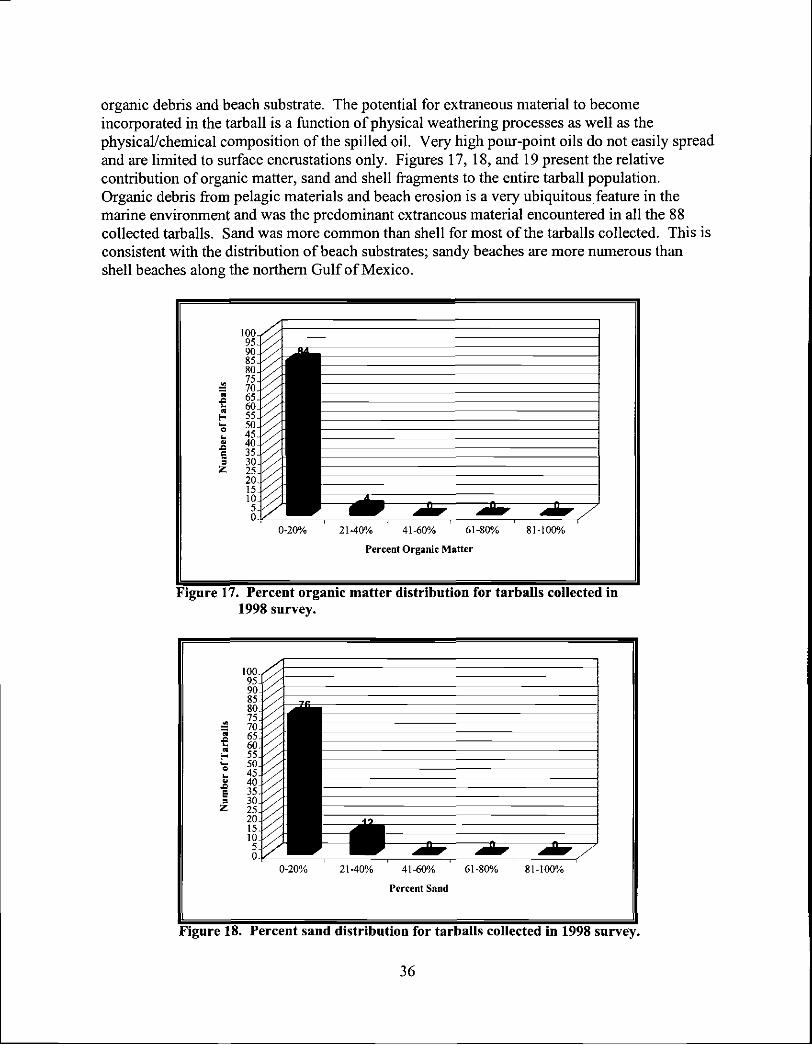
organic debris and beach substrate. The potential for extraneous material to becomeincorporated in the tarball is a function of physical weathering processes as well as thephysicallchemical composition of the spilled oil. Very high pour-point oils do not easily spreadand are limited to surface encrustations only. Figures 17, 18, and 19 present the relativecontribution of organic matter, sand and shell fragments to the entire tarball population.Organic debris from pelagic materials and beach erosion is a very ubiquitous feature in themarine environment and was the predominant extraneous material encountered in all the 88collected tarballs. Sand was more common than shell for most of the tarballs collected. This isconsistent with the distribution of beach substrates; sandy beaches are more numerous thanshell beaches along the northern Gulf of Mexico.

100959085807570656055504540353025201510

50

0-20% 21.40% 4l-60% 61-80% 81-l00%

Percent Organic Mailer

Figure 17. Percent organic matter distribution for tarballs collected in1998 survey.

100.95908580.757065

L 60a

I- 50C' 40i 35. 30Z2 SSa.rS/

0-20% 2140% 4h60% 6140% 81-100%

Percent Sand

Figure 18. Percent sand distribution for tarballs collected in 1998 survey.

36

353025201510

Figure 19. Percent shell distribution for tarballs collected in 1998 survey.

Each tarball was also characterized for its pliability. Pliability is generally associated with thephysical/chemical composition of the spilled oil and the extent of weathering which hasoccurred. Highly weathered tarballs tend to become nonpliable, often brittle or very difficult tobreak. These pliability characterizations were qualitative only. Each sample was rated from 0to 5. A rating score of 0 is nonpliable and nonbreakable using normal hand pressure. A scoreof 5 represents stranded tar that was almost fluid. Figure 20 displays the pliability score for thetarballs collected in 1998. The majority of the tarballs sampled for this research had a score of1, which represents tarballs that are difficult to bend with normal hand pressure. Less than 7%of the tarballs collected were nonpliable (score of 0) and none were scored as very fluid(pliability score of 5).

IZero One Two Three Four Five

Pliability Score

Figure 20. Tarball pliability score for 1998 samples.

37

90

80

70

60I.* 50

CI- 404.

E

z30

20

Analytical Chemistry Results

Of the 88 tarballs collected during the 1998 survey, 70 were sampled and analyzed by GCJMS.Eighteen samples were not extracted due to the fact that they were smaller than the cutoffweight established during the morphological characterization step of analysis; or were pieces ofasphalt too hard to sample. The first stage of data processing for the GC/MS analyses for eachof the 70 samples was classification into one of eight classifications adapted fromCharacterization of Chronic Sources and Impacts of Tar Along the Louisiana Coast (Henry etal. 1993). Some of the earlier classification schemes were based primarily on alkanes (Boehmet al. 1981), and more recently, polycyclic aromatic hydrocarbons (PAHs) classification havebeen published (Sauer et al. 1993). Any weathering classifications are most useful when theydescribe a specific oil type. The classification scheme used for this project consisted of eightcategories, which provided basic chemical information related to compositional change in thearomatic hydrocarbon fingerprint. The eight classifications are as follows:

Relatively unweathered, aromatic. Oils classified into this category were identifiedby a nC-18/phytane SF1 ratio of greater than 1 and were enriched with targetaromatic hydrocarbons. Oils in this classification are often representative of slightlyweathered, refined, blended fuel oils.

Relatively unweathered, paraffin. Oils classified into this category wereidentified by a nC-18/phytane SF1 ratio of grater than 1 and were enrichedwith normal paraffins between nC-iS and nC-33 often with the mostabundant normal paraffin being nC-19. Oils in this classification generally havehigh pour-points and many may be representative of heavy fuel oils.

Relatively unweathered, wax/bimodal wax. These tarballs are characterized by anC-18/phytane SF1 ratio greater than 1 and, in some instances, a bimodaldistribution of normal alkanes with a pronounce wax component from nC-21extending to nC-37. These oils are believed to be representative of crude oil andheavy fuel oil tank washings or sludge discharges.

Weathered, aromatic. Oils classified into this category were identified by a nC-1 8/phytane SF1 ratio of less than 1 and were enriched with target aromatichydrocarbons. Oils in this classification are often representative of weatheredrefined fuel oils and some highly weathered crude oils.

Weathered, paraffin. Oils classified into this category were identified by a nC-1 8/phytane SF1 ratio of less than 1 and were enriched with normal paraffins betweennC-15 and nC-33. Oils in this classification have high pour-points and many maybe derived from heavy, high pour-point fuel oils.

Weathered, wax/bimodal wax. These tarballs are characterized by a nC-i 8/phytaneratio less than 1 and in some instances, a bimodal distribution of normal alkaneswith a pronounced nC-21 extending to nC-37 wax component. These oils are

38

Visual Matching

An exhaustive matrix comparison process that utilized all the chromatographic data andprovided separation of the tarballs by source was the next step of the data interpretation. Thiscomparison involved visual scrutinization of each ion fingerprint for all biomarker ions chosenfor analysis. After analysis, a hard copy of all the ion fingerprints for each tarball was printedout and the biomarker ions were separated from the rest of the ions and stacked into separatepiles. Each tarball fingerprint in each pile was visually compared to each other to determine ifany matched or were nonmatches. Matched samples went into one pile and nonmatch samplesformed a new pile until every chromatogram had been compared. Each source was assigned analphabetical identification such as Source A and Source B. The comparisons were completedfor each tarball analyzed. Through this manual process and previous experience, certain ioncomponents within the samples were shown to be quite unique and descriptive.

believed to be representative of crude oil and fuel oil tank washings and sludgedischarges as noted from the unweathered bimodal wax.

Weathered, unresolved complex mixture (UCM). These tarballs are characterizedby a range of nC-18/phytane SF1 ratios and contain some normal alkanes andaromatic hydrocarbons, but could not be distinguished as weathered aromatic oils.All tarballs in this classification exhibited a large UCM in both the TIC and m/e 85.Oils in this classification are oflen highly weathered crude oils.

Unclassifiable. Oils that did not fit any of the above classifications. Generally,these oils were so heavily weathered, or not oils at all, that they could not beclassified with any confidence.

Table 11 provides a summary of the GC/MS tarball classifications for the samples analyzed inthe 1998 collection. The most common classification identified was weathered UCM, whichrepresented --57% of the samples analyzed. Figures 21, 22, 23, 24, 25, 26, and 27 showchromatographic ion fingerprints of oils typically classified as one of the eight categories,except Unclassified.

Table 11. Distribution of All Tarballs into Classifications.

Relatively UnweatheredAromatic

ParaffinWax/Bimodal Wax

Relatively WeatheredAromatic

ParaffinWax/Bimodal Wax

UCMUnclassifiable

Number ofSamples*

2

92

3

4012

% ofTotal--1.41.42.9

-42.9--2.94.3

5 7.1-47.1

39

(a)

(b)

Figure 21. Normal alkane distribution (a) and Total Ion Chromatogram(b) for a relatively unweathered, aromatic oil.

40

bundance140000-

120000-

100000-

80000 -

60000-

rime--> to.000LsLL44*JLø4:

Ion 85.00 (61.70 to 65.70): HP8195E.D

20.00 30.0 40.00 50 00 60.00 70.00

150000

140000

130000

120000

110000

100000

90000

000

70000

0000

50000

40000

30000

::::

time--s

-

I

-i4

TICt 00P295E0

J- 0 20.00 30.00 ,0. 00 50.00 60-00 '0-00

(a)

(b)

Figure 22. Normal alkane distribution (a) and Total Ion Chromatogram(b) for a relatively unweathered, paraffinic oil.

41

Ion., Q5.00 (84.70 to 65.10): H28161C.D

120000-

100000

60000 -

60000-

40000

2000:

rime--> io.00 20.00 30.00 40.00 50 00 60.00 70.00

thundaoca

500000

410000

400000

350000

300000

250000

200000

150000

100000

50 000

?j-->

TIC: H?eI6lC.D

10.00 20.00 30.00 40.00 SO 00 60.00 70.00

(a)

0')

Figure 23. Normal alkane distribution (a) and Total Ion Chromatogram(b) for a relatively unweathered, bimodal wax.

42

'ibundance

90000 -

80000 -

70000:

60000 -

50000-

40000 -

30000 -

20000-

1000:

rime-->r t4

Ion 85.00 (84.70 to 85.70): HP8169D.D

10.00 20.00 30.00 40.00 50.00 60.00 70.00

und.nc.

100000

95000

90000

65000

60000

75000

70000

65000

60000

55000

S0000

45000

40000

35000

30000

25000

20000

5000

TIC,

H

0800690.0

jTim.--> 10.00 10.00 3000 40.0 50.00 60.00 '0.00

(a)

(b)

Figure 24. Normal alkane distribution (a) and Total Ion Chromatogram(b) for a weathered, aromatic oil.

43

%bund&nca

50000-

45000-

400002

35000 -

30000-

25000

20000

15000

10000

5000-

Ion

-

85.00 (94.70 to 85.70): HP8162B.D

0 .. i...,Time--> 10.00 20.00 30. 0 40.00 50 00 60.00 70.00

,bu,dance

75000

70000

65000

60000

55000

50000

45000

40000

35000

30000

25000

20000

15000

10000

5000

0

TIne-->

TIC:

J-r

HP01620.D

p p I I'I10.00 20.00 30.00 40.00 50.00 40.00 '0.00

(a)

(b)

Figure 25. Normal alkane distribution (a) and Total Ion Chromatogram(b) for a weathered, paraffinic oil.

44

Zbundance

250000 -

200000-

150000 -

100000-

50000-

Ion 85.00 (84.70 to 85.7OhsHPO182D.D

time--> 10.000 '.,.. I

20.00 30.00 40.00 50.00 60.00 70.00

bundanc.

260000

240000

220000

200000

160000

160000

140000

20000

100000

10000

60000

40000

20000

71..-->

TIC, 10P11620.

10.00 20.00 30.00 40.00 00.00 60.00 70.00

(a)

(b)

Figure 26. Normal alkane distribution (a) and Total Ion Chromatogram(b) for a weathered, bimodal wax.

45

bundance300000-

250000

200000.

150000.

100000:

50000.

0Time-->

i1L110.00

Ion

_i[

85.00 (84.70 to 95.70); HP8161D.D

)20.00 30.00 40.00 50 00 60.00 70.00

bu,od.nc.

550000-

500000

450000-

400000 -

350000 -

300000.

250000-

200000

150000 -

'00000

5000:

Xl>

TIC. 01P31610.D

10.00 20.00 30.00 40.00 50 0 6 .00 70.00

(a)

(b)

Figure 27. Normal alkane distribution (a) and Total Ion Chromatogram(b) for a weathered, UCM.

46

bundance40000

35000-

30000-

25000 -

20000 -

15000 -

100o0-

5000

0

Ion 85.00 (64.70 to 85.70): HPB1Ø9C.D

Dime--) 10.00 20.00 30.00 40.00 50.00 60.00 70.00

untoc.40000

46000-

44 000-

42000-

40000-

30000

36000 -

34000 -

32000-

30000 -

20000 -

26000 -

24000.

22000-

20000

20000-

16000-

04000-

02000 -

10000 -

000G.

6200 -

4000-

2000LI i

TIC, 00P0109C.D

T0> 10.00 20.00 30. 0 40.0 50.00 6000 10 00

Source-fingerprinting of the 70 tarballs analyzed identified 66 different sources. Four matcheswere found through visual comparison and double SF1 scatterplots. The matches included onetarball matching Valvoline; one tarball matching ilondo Crude; one tarball matching SPRcrude; and two tarballs that matched each other but did not match one of the reference oils. Aninteresting observation is the wide distribution of sources from the three sampling locations.Apparently, the tarballs collected represent oil contamination from small petroleum and/orbilge waste discharge.

SF1 and Scatterplots

The initial group of SF1 scatterplots included all eight of the biomarkers chosen by IES/RCAT.As a result of the visual comparison, a selection of three of the SF1 were chosen and consistedof two SF1 per plot (i.e. C-3 Phen vs. C-3 DBT area/C-3 Phen area; and norhopane/hopane vs.the C-3 DBT areal C-3 Phen area). These indexes exhibited resistance to weathering during thewater degradation experiment and displayed chromatographic uniqueness. Figures 28 and 29are two examples of the double SF1 plots.

All the samples analyzed were plotted as a scatterplot in an attempt to further confirm sources.The reference oils prepared during the initial stages of the characterization and identification oftarballs were also plotted and target match zone were calculated based on a 20% standarddeviation of the SF1 chosen. A total of 29 possible matches, either to one of the reference oilsor to another tarball, were determined from the two different double SF1 scatterplots. However,only four of the matches were confirmed by visual comparison. Since the initial visualcomparison indicated an abnormal distribution of several non-related sources (66 differentsources), it was decided that principle component analysis would not provide the discriminationnecessary for statistical source-fingerprint results; therefore, scatterplots were created instead.Henry (1995) established that the use of principle component analysis did not provide thedegree of source resolution anticipated in a tarball population containing 67 different sources ina sample of 133. Had each source not been differentiated by visual comparison, identificationof which tarballs were related statistically could not be determined to any degree of confidence.Factors that contributed to the loss in discrimination included the limited value range of theindex values used and the extremely high number of different sources in the study population.Principle component analysis may have been useful if the study population demonstrated amore normal distribution.

The double SF1 scatter plots that were generated did not provide a high degree of identification,but were considered a useful screening tool. The resulting scatterplots were often moreconfusing than enlightening, yielding "inconclusive" results for all double SF1 plots attempted.The major factor influencing the interpretation of the scatterplots was the various stages ofweathering and sources for the tarballs sampled. Therefore, it has been concluded that doubleSF1 scatterplots are more efficient and defensible when one source oil and a few unknownsamples have been collected for analysis.

47

7

6

I

L

55

C3 Phenatithrene sIb10

xRefl0 .Martins Beach 1998

IS

Figure 28. C3 Phenanthrene versus C3 Dibenzothiophene/C3 Phenanthrene area doubleSF1 scatterplot for tarballs from Martin's beach.

4

.05

00 0' 02 03 04 0.5 06 01 08 09 10 II 12 3 14 IS 16 17 II 19 20

Norhopane/Hopane

xReference Oils Martins Beach 1998

Figure 29. Norhopanelllopane versus C3 Dibenzothiophene/C3 Phenanthrene area doubleSF1 scatterplot for tarbails from Martin's beach.

The SF1 values were validated for instrumental variability from the percent relative standarddeviation calculated from the daily North Slope Crude (NSC) reference oil. The %RSD for thedaily NSC ranged between 3.63 and 9.17%. Individual %RSD were as follows: nC-17/pristane, 3.63%; nC-18/phytane, 9.17%; C-3 DBT a/b, 6.08%; C-3 Phen a/b, 4.21%; c-iPyr a/b, 7.59%; C-I Chr a/b, 5.13%; Nor/Hop, 5.33%; and C-3 DBT area/C-3 Phen area,3.83%. One goal of this research was to choose SF1 that were unaffected by changes in

48

S0

instrumental operation. Each index, except for the C-3 DBT arealC-3 Phen area, was handcalculated on the basis of peak height rather than area to reduce integration error due to peaksnot being baseline resolved. The C-3 DBT arealC-3 Phen area SF1 is based on total arearepresented by each isomer group.

Of the 70 tarballs analyzed by detailed GC/MS, 57% had fingerprints indicative of weatheredcrude oils. The normal alkane distribution observed from the GC/MS analysis indicate that themajority of the weathered crude oils were a mid to heavy range. Light oils spilled in the marineenvironment spread very thinly on the water's surface and disperse by natural processes, suchas storms, and usually do not form tarballs. However, some of the tarballs were most likelyformed due to the formation of stable water-in-oil emulsifications, or mousses. Mousseformation is common for many crude oils and is a prime factor for the formation of tarballsfrom otherwise easily dispersible light crude oils. Very heavy crude oils are prone to formtarballs due to the fact that they are slow to spread and expose little surface area for naturaldegradation processes.

CONCLUSIONS AND RECOMMENDATIONS

Biomarker compounds, by definition, are universal in crude oils and petroleum products.These compounds are generally more resistant to environmental weathering than most of theother oil constituents. The distribution of biomarker compounds is unique for each oil anddifferent sources of petroleum exhibit different oil fingerprints. SF1 calculated from thesefingerprints provide a stable and useful tool for determining a match or nonmatch for differentoil residues present in some environmental samples. The presence and detection of biomarkercompounds is an indicator of some sort of oil exposure or contamination. Analytical chemistry,biomarker normalization determined by SF1, and visual comparisons of oil biomarkerfingerprints, provide environmental scientists with valuable information regarding theidentification of spilled oil and quantification of oil residues.

As far as general methodology is concerned, CC/MS operated in selected ion monitoring modeprovides detailed compositional and comprehensive information on saturated and aromatichydrocarbons, without requiring involved sample clean-up procedures prior to sampleextraction and analysis. High-resolution GC/MS analysis and source-fingerprinting techniqueswere employed throughout all experimental stages to validate and extend the use of biomarkersas tools for oil spill identification and assessment. Eight (8) petroleum biomarkers were chosenfor detection and analysis through a literature search and from previous research. Self-normalizing fingerprint indexes, or SF1, calculated from the GC/MS analysis of a waterdegradation experiment; a bioaccumulation study; and the classification and identification oftarballs assisted in the validation of the eight biomarkers chosen by LSU IES/RCAT.

Visual comparison played an important role in distinguishing gross, and in some cases subtle,differences in the biomarker fingerprints. This method is often the first step in GCIMS datainterpretation of spilled oil. Visual comparison of a small number of samples is very efficientfor matchlnonmatch determinations. A suggested method (Figure 30) for data interpretationsfor match/nonmatch determinations is as follows: print out hard copies of biomarker ions and

49

the TIC; separate each copy into separate biomarker ions; compare other copies of eachbiomarker ion to one another to determine a visual match/nonmatch; calculate the SF1 andcompare each value with the others in the group; plot the reference oil with the 20% targetmatch zone on one of the double index scatterplots from above and then plot the samples; andfinally, reconfirm matches with a visual comparison.

SF1 reflect the relative rates at which selected oil biomarkers are dissipated during thecombined physical, chemical, and biological processes that constitute oil weathering. Theeffects of weathering on the value of biomarker indexes are generally greatest in the periodinmediately following spillage or leakage. For SF1 to be valid throughout the weatheringprocesses, they must consist of components that are truly conserved during oil weathering andnot display significantly different physical properties (Whittaker and Pollard 1997). The SF1that meet this criterion and provide the best tool for oil spill identification, both visually andstatistically, are C-3 DBT, C-3 Phen, C-3 DBT area/C-3 Phen area, and Norhopane/Hopane.These compounds, as demonstrated by the water degradation experiment, remain stable evenafter weathering and will distinguish one oil source from another, even oils of similargeographical origin, when other biomarkers are lost (i.e. nC-17/Pris and nC-l8fPhy).

Generally, the simpler the chemical structure, the easier it is to degrade, which is the case fornC- 1 7/Pristane and nC- 1 8/Phytane. The latter two SF1 are straight-chain hydrocarbons that aremetabolized by microorganisms through successive oxidation and cleavage of terminal methylgroups of a hydrocarbon molecule. The C-3 DBT, C-3 Phen, C-3 DBT arealC-3 Phen area, andNorhopane/Hopane are branched or cyclic compounds that experience slowerbiotransformation rates due to the presence of secondary, tertiary, and quaternary carbon atomswithin the basic hydrocarbon structure, rendering them more difficult to metabolize (Whittakerand Pollard 1997).

Even though four of the eight SF1 are statistically valid, it is recommended that GC/MSanalysis and visual examination include all eight because they provide very valuableinformation about the extent of weathering and biodegradation from their respectivefingerprints. Visual examinations of chromatographic fingerprints provide very significantqualitative information, as opposed to the comparison of a few quantitative indexes, and caneasily distinguish one type of oil or weathering stage from another based on the pattern of thefingerprint alone.

One significant aspect of oil released on water is the ability of natural microbial communitieswithin the water to affect the oil composition; or in other words, their biodegradation potential.The key elements of biodegradation include the amount of oil, the mixing energy, the types ofmicrofauna, and the availability of oxygen. The water degradation experiment assessed theeffects of microorganism populations present in different water sources in two ways: BiologTMmicroplate analyses and percent reduction of total target aromatic hydrocarbons (TTAH). Theorganisms in the different water samples had widely varying metabolic capabilities.Unfortunately, the results from the BiologTM analyses and the %TTAH calculated from theGC/MS data did not correlate. This is due to several factors: differing carbon sources;differing nutrient substrates; and differing dominate microbial communities. However, theexperiment provided the best data in regards to the stability of the SF1 chosen by IES/RCAT.

50

Form one pile and designate as group "A'.

Print out hard copies of data.

Separate ions 85, 191, 216, 220,226, and 242 into six piles.

Calculate SF1 based on Figures 3-8.

VtCompare each sample in each ion pile to one another.

N

Label this sample with the same group designation (i.e. if' it matches A,lab& sample as A and pu in group A pile.

/Take next sample and compare to previous samples.

VDoes it match any of the other samples?

Plot SF1 and reference oil values on scatterplots.

VReconfirm matches by visual comparison.

Form two piles and designate as groups "A" and "B".

VLabel this sample as "C".

Figure 30. Suggested method for match/nonmatch determinations of unknown environmental oilsamples to a reference oil based on visual comparison and SF1 data.

51

Yes. No

NContinue on in the same manner with the rest of samples until finished.

VCalculate standard deviation and 200/ x -axis, y-axis values for reference oil.

The uptake of biomarkers and, in general PAHs, was examined in bivalves exposed to oil fromthe TN Exxon Valdez. Theoretically, biomarkers are not significantly altered by microbialdegradation, and since biomarkers are lipid soluble materials, they will accumulate in marineorganisms and could be used as an indicator of possible exposure during oil spills. Selectedmarine bivalves were collected during the 1999 NOAA Shoreline Monitoring Program ofPrince William Sound, Alaska and analyzed for PAH content and biomarker concentrations.The analysis provided important information about the uptake and utilization of petroleumhydrocarbons by filter feeding organisms after a duration of time (10 years) that would bedifficult to perform in a laboratory based experiment. Overall, the biomarker and PAHconcentrations for both mussel and clam tissues were low, and have been relatively low the pastfew years. Unfortunately, a baseline concentration of biomarker compounds has not beenestablished for biological samples from the beginning of the TN Exxon Valdez incident.

When spilled oil is weathered to the state of a tarball, the oil is generally considered lessacutely toxic than the fresh crude oil or the refined petroleum product from which it wasderived. This is due to the loss of the more water soluble mono- and di-aromatic hydrocarbons,such as the benzenes and naphthalenes, by evaporation and dissolution processes. However,tarballs are important environmental samples to analyze due to the fact that oil remaining in thetarball is enriched with the possible carcinogenic and chronically toxic 3,4, and 5 ring aromatichydrocarbons such as chiysene and benzo(a)pyrene.

The classification and identification of tarball samples collected in 1998 suggests that themajority of the tarballs collected were from mid- to heavy-range crude oil sources. Of the 70tarballs extracted and analyzed, four matches were found through visual comparison anddouble SF1 scatterplots. The double SF1 scatterplots were beneficial as a preliminaryidentification step of an unknown sample to a source oil. However, the various stages ofweathering and abnormal distribution of several non-related sources limited the scatterplotsability to discriminate, within defensible limits, a match or nonmatch to a source. Since thedistribution of sources was extensive, it is believed that the tarballs collected represent oilcontamination from small petroleum andlor bilge waste discharge.

In conclusion, the analysis of biomarker compounds can be further advanced through the use oftandem mass spectrometry. Triple-stage quadrupole (TSQ) mass spectrometers are currentlyavailable and several researchers have been developing new GC-MS/MS techniques for theanalysis of complex mixtures, such as oil and biomarker compounds above the nC-40 region(Philip and Oung 1988).

The water degradation experiment could be further advanced with a longer-term oil weatheringstudy. The duration of the study would be anywhere from one to two months. Several oilscould be tested in several types of natural waters and extracted and sub-sampled for microbialanalysis at select intervals throughout the experiment (i.e. days 0, 7, 14, 28, etc). Instrumentalanalysis would be by GCIMS or GC-MS7MS and data analysis would include calculation ofSF1. This would provide fingerprints of the various stages of weathering for each of the oilstested, which in turn, would be a valuable tool for oil spill responders. A more detailed studyof the microbial affects on oil could coincide with the longer-term weathering study andcharacterize the fluctuation of dominant species in the microbial population throughout the

52

study. This would include BiologTM characterization of the microbial communities present inthe waters and their ability to utilize a variety of carbon sources. The dominant communitiesidentified from the BiologTM analyses, using its carbon and nutrient sources, could then becompared to the dominant species identified from the sub-samples taken throughout the waterdegradation study. This analysis would clarify the differing results between the carbon sourceutilization from the BiologTM analyses and the GC/MS % reduction of petroleum hydrocarbons.

The important bioaccumulation factors that need further exploring are how bivalves metabolizepetroleum hydrocarbons throughout their life cycle. Generally, biomarker compounds areresistant to biodegradation, which implies bacterial degradation and not biologicaltransformation by the indigenous enzymes in the marine bivalves. A laboratory- simulated oilspill that would expose populations of mussels and clams to an oil would help establishconcentrations of the biomarker compounds throughout one to several life cycles of theanimals. Both Fl, biogenic fractions, and F2, PAH fractions, of the extracted tissues would beanalyzed by GC/MS or GC-MS/MS. Results from an experiment such as this would aidenvironmental scientists and oil spill responders in determining recent and conceivablyprevious oil exposure to biological specimens.

Developing more quantitative schemes for classifying and identifying tarballs would bedifficult due to the varying stages of weathering encountered throughout sampled populations.Double SF1 scatterplots and principle component analysis is one way of obtaining quantitativeschemes; however, they are most effective when there is only one source in question withseveral unknown samples. Further experimentation, such as the recommended waterdegradation study, could enhance the ability of scientists to develop more quantitative schemesfor classifying and identifying tarballs. At this point, classification of tarballs into different oilcompositions based on qualitative methods (i.e. morphological descriptions) and visualscrutinization of biomarker fingerprints remain the best tools for oil spill responders andenvironmental scientists.

LITERATURE CITED

Ahsan, A. and D.A. Karlsen. 1997. Petroleum biodegradation in the tertiary reservoirs of theNorth Sea. Marine and Petroleum Geology. l4(l):55-64.

Bochner, B.R. 1989. Sleuthing out bacterial identities. Nature. 339;157-158.

Boehm, P.D., D.L. Fiest, and A. Elskus. 1981. Comparative weathering patterns ofhydrocarbons from the Amoco Cadiz oil spill observed at a variety of coastalenvironments. In Amoco Cadiz, Fates and Effects of the Oil Spill Proceedings of the1981 International Symposium, Breat (France). pp. 159-173.

Butler, J.N., B.F. Moths, and J. Sass. 1973. Pelagic tar from Bermuda and the Sargasso Sea.Bermuda Biological Station Special PubI. No. 10.

53

Garland, J.L. and A.L. Mills. 1991. Classification and characterization of heterotrophicmicrobial comnunities on the basis of patterns of community-level sole-carbon-sourceutilization. Applied and Environmental Microbiology. 57:2351-2359.

Haack S K, H Garchow, M.J. KIug, and L.J. Fomey. 1995. Analysis of factors affecting theaccuracy, reproducibility, and interpretation of microbial community carbon sourceutilization patterns. Applied and Environmental Microbiology. 61:1458-1468.

Henry, C.B, P.O. Roberts, and E.B. Overton. 1993. Characterization of Chronic Sources andImpacts of Tar Along the Louisiana Coast. U.S. Dept. of the Interior, MineralsManagement Service, Gulf of Mexico OCS Regional Office, New Orleans, LA. OCSStudy MMS 93-0046. 64 pp.

Henry, C.B. 1995. Advancement of Forensic Petroleum Fingerprinting and Application ofGCIMS to Investigate Sources of Oil Pollution in the Marine Environment. MS thesis,Louisiana State University.

Overton, E.B, J. McFall, S.W. Mascarella, C.F. Steele, S.A. Antoine, JR. Politzer, and J.L.Laseter. 1981. Identification of petroleum residue sources after a fire and oil spill. InProceedings of the 1981 Oil Spill Conference. pp. 541-546.

Philip, R.P. and J.N. Oung. 1988. Biomarkers: Occurrence, Utility, and Detection. AnalyticalChemistry. 60(15):887A-896A.

Saucr, T.C., J.S. Brown, P.D. Boehm, D.V. Aurand, J. Michel, and MO. Hayes. 1993.Hydrocarbon source identification and weathering characterization of intertidal andsubtidal sediments along the Saudi Arabian coast after the Gulf War oil spill. MarinePollution Bulletin. 27:117-134.

Sauer, T. and P. Boehm. 1991. The use of defensible analytical chemical measurements for oilspill natural resource damage assessment. In Proceedings of the 1991 Oil SpillConference. pp. 363-369.

Smalla, K., U. Wachtendorf, H. Heuer, W-T Liu, and L. Fomey. 1998. Analysis of BIOLOGGN Substrate Utilization Patterns by Microbial Communities. Applied andEnvironmental Microbiology. 64: 1220-1225.

Wang, Z. and M. Fingas. 1995a. Chemical analysis methods for crude oil. In Proceedings ofthe 1995 Oil Spill Conference. pp. 1004-1006.

Wang, Z. and M. Fingas. 1995b. Using biomarker compounds to track the source of spilled oiland to monitor the oil weathering process. LC/GC. 13(2):951-958.

Whittaker, M. and S.J.T. Pollard. 1997. A performance assessment of source correlation andweathering indices for petroleum hydrocarbons in the environment. EnvironmentalToxicology and Chemistry. 16(6): 1149-1158.

54

Wunsche, L., L. Bruggemann, and W. Babel. 1995. Determination of substrate utilizationpatterns of soil microbial communities: An approach to assess population changes afterhydrocarbon pollution. FEMS Microbiology Ecology. 17:295-306.

55

APPENDIX

Biomarkers of Petroleum Products in the Marine Environment: A Bibliography.

57

APPENDIXBiomarkers of Petroleum Products in the Marine Environment: A Bibliography

Abdullah, A. R., W. C. Woon, et al. (1996). "Distribution of Oil and Grease and PetrolemHydrocarbons in the Straits of Johor, Peninsular Malaysia." Bulletin ofEnvironmental Contamination and Toxicology 57: 155-162.

Aboul-Kassim, T. A. T. and B. R. T. Simoneit (1995). "Petroleum HydrocarbonFingerprinting and Sediment Transport Assessed by Molecular Biomarker andMultivariate Statistical Analyses in the Eastern Harbour of Alexandria, Egypt."Marine Pollution Bulletin 30(1): 63-73.

Aboul-Kassim, T. A. T. and B. R. T. Simoneit (1996). "Lipid Geochemistry of SurficialSediments from the Coastal Environment of Egypt I. Aliphatic Hydrocarbons -Characterization and Sources." Marine Chemistry 54: 135-158.

Ahsan, A., D. A. Karisen, et al. (1997). "Petroleum Biodegradation in the TertiaryReservoirs of the North Sea." Marine and Petroleum Geology 14(1): 55-64.

Alajbeg, A., V. Britvic, et al. (1990). "Geochemical Study of the Oils and Source Rocksin the Pannonian Basin (Yugoslavia)." Organic Geochemistry 16(1-3): 339-352.

Albaiges, J. and P. Albrecht (1979). "Fingerprinting Marine Pollutant Hydrocarbons byComputerized Gas Chromatography-Mass Spectrometry." International Journal ofEnvironmental Analytical Chemistry 6: 171-190.

Alexander, R., R. I. Kagi, et al. (1994). "The Effect of Maturity on the RelativeAbundances of Cadalene and Isocadalene in Sediments from the Gippsland Basin,Australia." Organic Geochemistry 21(2): 115-120.

Al-Hadhrami, M. N., H. M. Lappin-Scott, et al. (1996). "Effects of the Addition ofOrganic Carbon Sources on Bacterial Respiration and n-Alkane Biodegradation ofOmani Crude Oil." Marine Pollution Bulletin 32(4): 35 1-357.

Ali, L. N., R. Fauzi, et al. (1995). "The Dissolution and Photodegradation of KuwaitiCrude Oil in Seawater. Part 1: Quantitative Dissolution and Analysis of theSeawater-Soluble Fraction." Marine Envirionmental Research 40(1): 1-17.

Ali, L. N., R. F. Mantoura, et al. (1995). "The Dissolution and Photodegradation ofKuwaiti Crude Oil in Seawater. Part 2: A Laboratory PhotodegradationApparatus and Photodegradation Kinetics of a Model Seawater SolubleHydrocarbon (Phenanthrene)." Marine Environmental Research 40(4): 3 19-335.

Andersen, B. (1990). "Fingerprinting Petroleum Problems." Energy andTechnology(July-August'): 90.

Anderson, B. (1994). Elimination of Chemicals Urged. The Advocate. Baton Rouge, LA:2B.

Anderson, C. B. and B. D. Starer (1990). "Contingency Planning Crucial to Oil-SpillResponse." Oil and Gas Journal OGJ Special(March): 41-42,44,46.

Armanios, C., R. Alexander, et al. (1994). "Fractionation of Sedimentary Higher-PlantDerived Pentacyclic Triterpanes Using Molecular Sieves." Organic Geochemistry21( 5): 53 1-543.

Armstrong, D. W., Y. Tang, et al. (1991). "Resolution of Enantiometric HydrocarbonBiomarkers of Geochemical Importance." Analytical Chemistry 63: 2858-2861.

59

Atlas, R. M., P. D. Boehm, et al. (1981). "Chemical and Biological Weathering of Oil,from the Amoco Cadiz Spillage, within the Littoral Zone." Estuarine, Coastal andShelf Science 12: 589-608.

Baker, J. M. (1970). The Effects of a Single Oil Spillage. Ecological Effects of OilPollution on Littoral Communities. E. B. Cowell: 16-20.

Baker, J. M. (1971). Successive Spillages. Ecological Effects of Oil Pollution on LittoralCommunities. E. B. Cowell: 2 1-32.

Baker, J. M., L. M. Guzman, et al. (1993). Long-Term Fate and Effects of UntreatedThick Oil Deposits on Salt Marshes. 1993 Oil Spill Conference.

Beiger, T., J. Hellou, et al. (1996). "Petroleum Biomarkers as Traces of Lubricating OilContamination." Marine Pollution Bulletin 32(3): 270-274.

Benner, B. A., Jr., N. P. Bryner, et al. (1990). "Polycyclic Aromatic HydrocarbonEmissions from the Combustion of Crude Oil on Water." Environmental Science& Technology 24(9): 1418-1427.

Bernard, D., H. Pascaline, et al. (1996). "Distribution and Origin of Hydrocarbons inSediments from Lagoons with Fringing Mangrove Communities." MarinePollution Bulletin 3200): 734-739.

Blumer, M. and S. Jeremy (1972). "Oil Pollution: Persistence and Degradation of SpilledFuel Oil." Science 176: 1120-1122.

Boehm, P. D. (1989). Exxon Valdez Chemistry Program: Recommended Procedure forthe Chemical Analysis of Oil, Mousse, and Tarball Samples and the Use of Datain Determinations of Source and Weathering Extent.

Boehn, P. D., H. J. Costa, et al. (1994). Assessment of the Changes in Composition andConcentration of Spilled San Joaquin Valley Crude Oil and Bioavailability ofSpilled Oil Residues in Suisan Bay Sediments.

Boehni, P. D., 0. 5. Douglas, et al. (1995). Advanced Chemical Fingerprinting for OilSpill Identifications and Natural Resource Damage Assessments. 1995International Oil Spill Conference, Long Beach, CA.

Boehm, P. D. and J. W. Farrington (1984). "Aspects of the Polycyclic AromaticHydrocarbon Geochemistry of Recent Sediments in the Georges Bank Region."Environmental Science & Technology 18(11): 840-845.

Boehni, P. D., D. L. Fiest, et al. (1981). Comparative Weathering Patterns ofHydrocarbons From the Amoco Cadiz Oil Spill Observed at a Variety of CoastalEnvironments. International Bolume on the Amoco Cadiz: Fate and Effects ofthe Oil Spill, Brest, France, Brest, France.

Boehm, P. D., J. C. Foster, et al. Monitoring Chemical Fate of Spilled Oil: 19-107.Boehm, P. D., P. J. Mankiewicz, et al. (1996). "Characterization of Mussel Beds With

Residual Oil and the Risk to Foraging Wildlife 4 Years After the Exxon ValdezOil Spill." Environmental Toxicology and Chemistry 15(8): 1289-1303.

Boehm, P. D. and J. 0. Quinn (1976). "The Effect of Dissolved Organic Matter in SeaWater on the Uptake of Mixed Individual Hydrocarbons and Number 2 Fuel Oilby a Marine Filter-feeding Bivalve (Mercenaria mercenaria )." Estuarine andCoastal Marine Science 4: 93-105.

60

Bogan, B. W. and R. T. Lemar (1996). "Polycyclic Aromatic Hydrocarbon-DegradingCapabilities of Phanerochaete laevis HHB-1625 and Its ExtracellularLigninolytic Enzymes." Applied and Environmental Microbiology 62(5): 1597-1603.

Boon, J. J., F. W. Meer, et al. "Organic Geochemical Analysis of Core Samples from Site362, Walvis Ridge, DSPS Leg 40.": 627-637.

Borzelli, G., A. Ciappa, et al. (1996). "A New Perspective on Oil Slick from Space byNOAA Satellites." International Journal of Remote Sensing 17(7): 1279-1292.

Brakstad, F. and 0. Grahl-Nelson (1988). "Identification of Weathered Oils." MarinePollution Bulletin 19(7): 3 19-324.

Broman, D., A. Colmsjo, et al. (1987). "Fingerprinting' Petroleum Hydrocarbons inBottom Sediment, Plankton, and Sediment Trap Collected Seston." MarinePollution Bulletin 18(7): 380-388.

Brown, J. S. and P. D. Boehm The Use of Double Ratio Plots of Polynuclear AromaticHydrocarbon (PAH) Alkyl Homologues for Petroleum Source Identifiction.

Bruheim, P., H. Bredholt, et al. (1997). "Bacterial Degradation of Emulsified Crude Oiland the Effect of Various Surfactants." Canadian Journal of Microbiology 43: 17-22.

Burns, W. A., P. J. Mankiewicz, et al. (1997). "A Principal-Component and Least-Squares Method for Allocating Polycyclic Aromatic Hydrocarbons in Sediment toMultiple Sources." Environmental Toxicology and Chemistry 16(6): 1119-1131.

Chosson, P., C. Lanau, et al. (1991). "Biodegradation of Refractory HydrocarbonBiomarkers from Petroleum Under Laboratory Conditions." Nature 351(June 20):640-642.

Colombo, J. C., E. Pelletier, et al. (1989). "Determination of Hydrocarbon Sources Usingn-Alkane and Polyaromatic Hydrocarbon Distribution Indexes. Case Study: Riode La Plata Estuary, Argentina." Environmental Science & Technology 23(7):888-894.

Conde, J. E., E. Pena, et al. (1996). "Sources of Tar Balls and Oil Slicks on the Coasts ofthe Canary Islands." International Journal of Environmental and AnalyticalChemistry 62: 77-84.

Connan, J. (1984). Biodegradation of Crude Oils in Reservoirs. Advances in PetroleumGeochemistry. J. Brooks and D. Welte. London, Academic Press (Harcourt BraceJovanovich). 1: 299-335.

Curiale, J. A. and B. W. Bromley (1996). "Migration Induced Compositional Changes inOils and Condensates of a Single Field." Organic Geochemistry 24(12): 1097-1113.

Curl, H. J. and K. O'Doimell (1977). Chemical and Physical Properties of RefinedPetroleum Products, United States Department of Commerce.

DahI, D. (1993). A New Weapon in Environmental Cases "Chemical Fingerprinting"Traces an Oil Spill's Origins. Lawyers Weekly USA: B3.

Dahl, J., J. M. Moldowan, et al. (1992). "A New Class of Natural Products Revealed by3B-Alkyl Steranes in Petroleum." Nature 355(January): 154-157.

D'Elia, C. F., J. G. Sanders, et al. (1989). "Analytical Chemistry for EnvironmentalSciences." Environmental Science and Technology 23(7): 768-774.

61

Dingchuang, Q., S. Jiyang, etal. (1996). "Novel Extended Side-Chain-UnsaturatedReleased from the Kerogen Macromolecules under Artificial Conditions."Organic Geochemistry 24(89): 8 15-823.

Disnar, J. R. and M. Harouna (1994). "Biological Origin of Tetracyclic Diterpanes, n-alkanes and Other Biomarkers Found in Lower Carboniferous Gondwana Coals(Niger)." Organic Geochemistry 21(2): 143-152.

Dixon, I. (1996). "Photoacoustic Monitoring of Oil Pollutants." Marine Pollution Bulletin32(6): 454-455.

Douglas, G. S., A. E. Bence, et al. (1996). "Environmental Stability of SelectedPetroleum Hydorcarbon source and Weathering Ratios." Environmental Scienceand Technology 30: 2332-2339.

Douglas, G. S., R. C. Prince, et al. (1994). The Use of Internal Chemical Indicators inPetro!eum and Refined Products to Evaluate the Extent of Biodegradation.Hydrocarbon Bioremediation. R. E. Hinchee, B. C. Alleman, R. E. Hoppel and R.N. Miller. Ann Arbor, MI, Lewis Publishers: 219-235.

Douglas, G. S. and A. D. Uliler (1993). "Optimizing EPA methods for Petroleum-Contaminated Site Assessments." Environmental Testing andAnalysis(May/June): 1-6.

Draper, W. M., J. S. Dhaliwal, et al. (1996). "Determination of Diesel Fuel and Motor Oilin Water and Wastes by a Modified Diesel-Range Organics Total PetroleumHydrocarbon Method." Journal of AOAC International 79(2): 509-5 19, 629-632.

Ehrhardt, M. G. and K. A. Bums (1990). "Petroleum-Derived Dissolved OrganicCompounds Concentrated from Inshore Waters in Bermuda." Journal ofExperimental Marine Biology and Ecology 138: 35-47.

Ellis, L., R. K. Singh, et al. (1996). "Formation of Isohexyl Alkylaromatic Hydrocarbonsfrom Aromatization-Rearrangement of Terpenoids in the SedimentaryEnviornment. A New Class of Biomarker." Geochimica et Cosmochimica Acta60(23): 4747-4763.

Essaid, H. I., B. A. Bekins, etal. (1995). "Simulation of Aerobic and AnaerobicBiodegradation Processes at a Crude Oil Spill Site." Water Resources Research31(12): 3309-3327.

Farrington, J. (1992). "Biomarker and Molecular Paleontology Working Group Report."Marine Chemistry 39: 5 1-65.

Fayad, N. M. and E. Overton (1995). "A Unique Biodegradation Pattern of the OilSpilled During the 1991 Gulf War." Marine Pollution Bulletin 30(4): 239-246.

Fazeelat, T., R. Alexander, etal. (1994). "Extended 8,14-Secohopanes in Some Seep OilsFrom Pakistan." Organic Geochemistry 21(3/4): 257-264.

Fingas, M. (1995). The Evaporation Oil Spills. Proceedings of the Eighteenth Artic andMarine Oilspi!l Program (AMOP) Technical Seminar, Edmonton, Alberta,Canada, Environment Canada.

Fingas, M. (1996). The Evaporation of Oil Spills: Variation with Temperature andCorrelation with Distillation Data Proceedings of the Nineteenth Artic andMarine Oi!spill Program (AMOP) Technical Seminar, Calgary, Alberta, Canada,Environment Canada.

Frank, U., D. Stainken, et al. (1979). Methods for the Source Identification andQuantification of Oil Pollution. 1979 Oil Spi!! Conference.

62

Gerlach, C. L. (1996). "New Instrument Brings PAH Analysis to the Field."Environmental Science and Technology (Featured Article) 30(6): 252A-254A.

Glegg, G. A. and S. J. Rowland (1996). "The Braer Oil Spill - HydrocarbonConcentrations in Intertidal Organisms." Marine Pollution Bulletin 32(6): 486-492.

Goodwin, N. S., P. J. D. Park, et al. (1981). "Crude Oil Biodegradation under Simulatedand Natural Conditions." Advances in Organic Chemistry: 650-658.

Grantham, P. J. and L. L. Wakefield (1988). "Variations in the Sterane Carbon NumberDistributions of Marine Source Rock Derived Crude Oils through GeologicalTime." Organic Geochemistry 12(1): 61-73.

Grigson, S. and G. Baron (1993). The European Approach to the Source Identification ofOil Spills: A Study of its Specificity and Reliability. 1993 International Oil SpillConference, Tampa, FL, American Petroleum Institute.

Harkey, G. A., P. L. V. Hoof, et al. (1995). "Bioavailability of Polycyclic AromaticHydrocarbons from a Historically Contaminated Sediment Core." EnvironmentalToxicology and Chemistry 14(9): 155 1-1560.

Hartley, J. P. (1996). "Environmental Monitoring of Offshore Oil and Gas DrillingDischarges-A Caution on the Use of Barium as a Tracer." Marine PollutionBulletin 32(10): 727-733.

Hayes, M. 0., J. Michel, etal. (1993). "Distribution of Oil From the Gulf War SpillWithin Intertidal Habitats-One Year Later." Oil Spill Conference: 373-381.

Hellebust, J. A., B. Hamia, et al. (1975). Experimental Crude Oi! Spills on a SmallSubarctic Lake in the Mackenzie Valley, N.W.T.: Effects on Phytoplankton,Periphyton, and Attached Aquatic Vegetation. Proceedings of the 1975 Oil SpillConference (Prevention, Behavior, Control, Cleanup).

Henry, C. B., Jr. and E. B. Overton (1993). Chemical Composition and SourceFingerprinting of Depositonal Oil from the Kuwait Oil Fires. 1993 InternationalOil Spill Conference, Tampa, FL, American Petroleum histitute.

Henry, C. B., Jr. and E. B. Overton (1993). Source-Fingerprinting and CompoundSpecific Quantitative Analysis of Oil Contaminated Soils and Sediments, Institutefor Environmental Studies Louisiana State University.

Henry, C. B., Jr., E. B. Overton, et al. (1990). Standard Method: Source-FingerprintAnalysis of Moderate to Heavily Contaminated Samples Associated with theExxon Valdez.

Henry, C. B., P. 0. Robert, et al. (1993). Characterization of Chronic Sources andImpacts of Tar along the Louisiana Coast, Institute for Environmental Studies,Louisiana State University.

Horstad, I., S. R. Larter, et al. (1989). "Degradation and Maturity Controls on Oil FieldPetroleum Colunm Heterogeneity in the Gullfaks Field, Norwegian North Sea."Advances in Organic Geochemistry 16(1-3): 497-510.

Hostetticr, F. D. and K. A. Kvenvolden (1994). "Geochemical Changes in Crude OilSpilled from the Exxon Valdez Supertanker into Prince William Sound, Alaska."Organic Geochemistry 21(8/9): 927-936.

Hostettler, F. D., J. B. Rapp, et al. (1992). "Use of Geochemical Biomarkers in BottomSediment to Track Oil from a Spill, San Francisco Bay, California." MarinePollution Bulletin 24(1): 15-20.

63

Hund, K. and W. Traunspurger (1994). "Ecotox-Evaluation Strategy for SoilBioremediation Exemplified for a PAH-Contaminated Site." Chemosphere 29(2):37 1-390.

Hwang, R. J., A. S. Ahmed, et al. (1994). "Oil Composition Variation and ReservoirContinuity: Unity Field, Sudan." Organic Geochemistry 21(2): 171-188.

Jacob, J. (1996). "The Significance of Polycyclic Aromatic Hydrocarbons asEnvironmental Carcinogens." Pure and Applied Chemistry 68(2): 301-308.

Jacquot, F., M. Guiliano, et al. (1996). "In Vitro Photooxidation of Crude Oil MaltenicFractions: Evolution of Fossil Biomarkers and Polycyclic AromaticHydrocarbons." Chemosphere 33(4): 671-681.

Kanga, S. A., J. S. Boimer, et al. (1997). "Solubilization of Naphthalene and Methyl-Substituted Naphthalenes from Crude Oil Using Biosurfantants." EnvironmentalScience and Technology 31: 556-561.

Kayal, S. and D. W. Comiell (1995). "Polycyclic Aromatic Hydrocarbons in Biota fromthe Brisbane River Estuary, Australia." Estuarine, Coastal, and Shelf Science40(5): 475-493.

Kennicutt, M. C., 11(1988). "The Effect of Biodegradation on Crude Oil Bulk andMolecular Composition." Oil & Chemical Pollution 4: 89-112.

Khalili, N. R., P. A. Scheff, et al. (1995). "PAH Source Fingerprints for Coke Ovens,Diesel and Gasoline Engines, Highway Tunnels, and Wood CombustionEmissions." Atmospheric Environment 29(4): 533-542.

Killops, S. D., M. S. Massoud, et al. (1991). "Biomarker Characterisation of an Oil andits Possible Source Rock from Offshore Korea Bay Basin." AppliedGeochemistry 6: 143-157.

Komacki, A. S., J. W. Kendrick, et al. (1994). "Impact of Oil and Gas Vents and Slickson Petroleum Exploration in the Deepwater Gulf of Mexico." Geo-Marine Letters14(2/3): 160-169.

Kropp, K. G., J. A. Goncalves, et al. (1994). "Bacterial Transformations ofBenzothiophene and Methylbenzothiophenes." Environmental Science andTechnology 28: 1348-1358.

Kueklick, J. R., S. K. Siversten, et al. (1997). "Factors Influencing Polycyclic AromaticHydrocarbon Distributions in South Carolina Estuarine Sediments." Journal ofExperimental Marine Biology and Ecology 213: 13-29.

Kvenvolden, K. A., P. R. Carlson, et al. (1993). "Possible Connection Between TwoAlaskan Catastrophes Occuring 25 yr Apart (1964 and 1989)." Geology 21: 813-816.

Kvenvolden, K. A., F. D. Hostettler, et al. (1993). "Hydrocarbons in Oil Residues onBeaches of Islands of prince William Sound, Alaska." Marine Pollution Bulletin26(1): 24-29.

Lavine, B. K., H. Mayfield, et al. (1995). "Source Identification of Underground FuelSpills by Pattern Recognition Analysis of High-Speed Gas Chromatograms."Analytical Chemistry 67: 3846-3852.

Law, R. J. and J. L. Biscaya (1994). "Polycyclic Aromatic Hydrocarbons (PAM)-Problems and Progress in Sampling, Analysis and Interpretation." MarinePollution Bulletin 29(4-5): 235-241.

64

Li, M., S. R. Latter, et al. (1995). "Biomarkers or Not Biomarkers? A New Hypothesisfor the Origin of Pristane Involving Derivation fromMethyltrimethyltridecyichomans (MTTCs) Formed during Diagenesis fromChlorophyll and Alkyiphenols." Organic Geochemistry 23(2): 159-167.

Licht, D., B. K. Ahring, et al. (1996). "Effects of Electron Acceptors, Reducing Agents,and Toxic Metabolites on Anaerobic Degradation of Heterocyclic Compounds."Biodegradation 7: 83-90.

Mackenzie, A. S. (1984). Applications of Biological Markers in PetroleumGeochemistry. Advances in Petroleum Geochemistry. J. Brooks and D. Welte.London, Academic Press (Harcourt Brace Jovanovich). 1: 115-214.

Marshall, K. C. (1980). "Microorganisms and Interfaces." BioScience 30(4): 246-249.Martin, G. (1991). "Marked for Life." Discover: 28.McCaffrey, M. A., B. R. T. Simoneit, et al. (1994). "Functionalized Biological Precursors

of Tricyclic Terpanes: Information from Sulfur-bound Biomarkers in a PermianTasmanite." Organic Geochemistry 21(5): 48 1-487.

McGee, B. L., C. E. Schlekat, et al. (1995). "Sediment Contamination and BiologicalEffects in a Chesapeake Bay Marina." Ecotoxicolgy 4: 39-59.

Mello, M. R., P. C. Gaglianone, et al. (1988). "Geochemical and Biological MarkerAssessment of Depositional Environments using Brazilian Offshore Oils." Marineand Petroleum Geology 5(August): 205-223.

Morel, G. (1996). "Method Development and Quality Assurance for the Analysis ofHydrocarbons in Environmental Samples." International Journal ofEnvironmental Analytical Chemistry 63: 269-288.

Neff, J. M. and W. A. Burns (1996). "Estimation of Polycyclic Aromatic HydrocarbonConcentrations in the Water Column Based on Tissue Residues in Mussels andSalmon: An Equilibrium Partitioning Approach." Environmental Toxicology andChemistry 15(12): 2240-2253.

Nichols, P. D., D. S. Nichols, et al. (1993). "Recent Developments with Marine OilProducts in Australia." Chemistry in Australia(July): 336-340.

Overton, E. B., J. McFalls, et al. (1981). Identification of Petroleum Residue SourcesAfter A Fire And Oil Spill. 1981 Oil Spill Conference, Atlanta, GA.

Owens, E. H. (1984). "Variablility in Estimates of Oil Contamination in the IntertidalZone of a Gravel Beach." Marine Pollution Bulletin 15(11): 412-416.

Page, D. S., P. D. Boehm, et al. (1993). "Identification of Hydrocarbon Sources in theBenthic Sediments of Prince William Sound and the Gulf of Alaska Following theExxon Valdez Oil Spill." Aquatic, Plant and Terrestrial(April 26-28): 1-42.

Page, D. S., P. D. Boehm, et al. (1996). "The Natural Petroleum HydrocarbonBackground in Subtidal Sediments of Prince William Sound, Alaska, USA."Environmental Toxicology and Chemistry 15(8): 1266-1281.

Parsons, K. C. (1996). "Recovering from Oil Spills: The Role of Proactive Science inMitigating Adverse Effects." Colonial Waterbirds 19(1): 149-153.

Peters, K. E. and J. M. Moldowan (1991). "Effects of Source, Thermal Maturity, andBiodegradation on the Distribution and Isomerization of Homohopanes inPetroleum." Organic Geochemistry 17(1): 47-61.

Peters, K. E., 0. L. Scheuerman, et al. (1992). "Effects of Refinery Processes onBiological Markers." Energy & Fuels 6: 560-577.

65

Philip, R. P., J. N. Oung, et at. (1990). "The Determination of Biomarker Distributions byTandem Mass Spectrometry." Advances in Organic Geochemistry (OrganicGeochemistry) 16(4-6): 1211-1220.

Philp, R. P. and J.-N. Oung (1988). "Biomarkers." Anaytical Chemistry 60(15): 887A-896A.

Pieri, N., F. Jaquot, Ct al. (1996). "GC-MS Identification of Biomarkers in Road Asphaltsand in Their Parent Crude Oils. Relationships Between Crude Oil Maturity andAsphalt Reactivity Towards Weathering." Organic Geochemistry 25(1/2): 5 1-68.

Porter, P. S., R. C. Ward, et al. (1988). "The Detection Limit." Environmental Science &Technology 22(8): 856-861.

Prahl, F. G., L. A. Pinto, et al. (1996). "Phytane from Chemolytic Analysis of ModemMarine Sediments: A Product of Desulffirization or Not?" Geochimica etCosmochimica Acta 60(6): 1065-1073.

Pu, F., R. P. Philp, et al. (1990). "Geochemical Characteristics of Aromatic Hydrocarbonsof Crude Oils and Source Rocks from Different Sedimentary Environments."Organic Geochemistry 16(1-3): 427-435.

Quinn, M. F., K. Marron, et al. (1990). "Modelling of the Ageing of Crude Oils." Oil andChemical Pollution 7: 119-128.

Radke, M., P. Garrigues, et al. (1990). "Methylated Dicyclic and Tricyclic AromaticHydrocarbons in Crude Oils from the Handil Field, Indonesia." OrganicGeochemistry 15W: 17-34.

Readman, J. W., J. Bartocci, et al. (1996). "Recovery of the Coastal Marine Environmentin the Gulf Following the 1991 War-Related Oil Spills." Marine PollutionBulletin 32(6): 493-498.

Readman, J. W., S. W. Fowler, et al. (1992). "Oil and Combustion-ProductContamination of the Gulf Marine Environment following the War." Nature358(August): 662-665.

Readman, J. W., I. Tolosa, et al. (1996). "Discrete Bands of Petroleum Hydrocarbons andMolecular Organic Markers Identified Within Massive Coral Skeletons." MarinePollution Bulletin 32(5): 437-443.

Reed, W. E. (1977). "Molecular Compositions of Weathered Petroleum and Comparisonwith its Possible Source." 41: 237-247.

Reilley, K. A., M. K. Banks, et al. (1996). "Organic Chemicals in the Enviornment."Journal of Environmental Quality 25(2): 212-219.

Requejo, A. G., R. Sassen, et al. (1996). "Polynuclear Aromatic Hydrocarbons (PAR) asIndicators of the Source of Maturity of Marine Crude Oils." OrganicGeochemistry 24(10/1 1): 1017-1033.

Ricimow, H. H., R. Seifert, et al. (1995). "Rapid Screening of PAH-Residues inBioremediated Soils." Chemosphere 31(8): 3991-3999.

Riediger, C. L., M. G. Fowler, et al. (1990). "Triassic Oils and Potential Mesozoic SourceRocks, Peace River Arch Area, Western Canada Basin." Organic Geochemistry16(1-3): 295-305.

Roberts, P. 0., C. B. Henry, et al. (1995). Fast Source-Fingerprinting Analysis for OilSpill Response. 1995 International Oil Spill Conference, Long Beach, CA,American Petroleum Institute.

66

Roques, D. E., E. B. Overton, et al. (1994). "Using Gas Chromatography/MassSpectroscopy Fingerprint Analyses to Document Process and Prograss of OilDegradation." Journal of Environmental Quality 23(4): 85 1-855.

Rulikotter, J., C. Comford, et al. Organic Geochemistry of Sediments Cored During DeepSea Drilling Project Legs 56 and 57, Japan Trench: Organic Petrography andExtractable Hydrocarbons.

Saliot, A., C. Andrie, et al. (1986). Hydrocarbons in the Mediterranean Sea: TheirOccurrence and Fate in the Sediment and in the Water Column, as Dissolved andAssociated with Small and Large Size Particulates. Fate of Hydrocarbons in theEnvironment: An Analytical Approach. J. Albaiges and R. W. Frei. New York,New York, Gordon and Breach Science: 255-276.

Saliot, A., J. Laureillard, et al. (1991). "Evolutionary Trends in the Lipid BiomarkerApproach for Investigating the Biogeochemistry of Organic Matter in the MarineEnvironment." Marine Chemistry 36: 223-248.

Salmeen, I. T., B. R. Kim, et al. (1995). "Case of Lognormally Distributed TPH inContaminated Soil." Journal of Environmental Engineering 121(9): 664-667.

Sauer, T. and P. Boehm (1991). The Use of Defensible Analytical ChemicalMeasurements for Oil Spill Natural Resource Damage Assessment. 1991 Oil SpillConference.

Sauer, T. C. and A. D. Ubler (1994). "Pollutant Source Identification and Allocation:Advances in Hydrocarbon Fingerprinting." Remediation(Winter): 25-50.

Saxton, W. L., R. T. Newton, et al. (1993). "Polycyclic Aromatic Hydrocarbons inSeafood from the Gulf of Alaska Following a Major Crude Oil Spill." Bulletin ofEnvironmental Contamination and Toxicology 51(4): 5 15-522.

Schoell, M. (1984). Stable Isotopes in Petroleum Research. Advances in PetroleumGeochemistry. J. Brooks and D. Welte. London, Academic Press (Harcourt BraceJovanovich). 1: 215-245.

Seifert, W. K. and J. M. Moldowan (1979). "The Effect of Biodegradation on Steranesand Terpanes in Crude Oils." Geochimica et Cosmochimica Acta. 43: 111-126.

Seifert, W. K., J. M. Moldowan, et al. (1984). "Source Correlation of Biodegraded Oils."Organic Geochemistry 6: 633-643.

Seifert, W. K. and J. M. Moldwan (1978). "Applications of Steranes, Terpanes andMonoaromatics to the Maturation, Migration and Source of Crude Oils."Geochimica et Cosmochimica Acta 42: 77-95.

Shen, J. (1984). "Minimization of Interferences from Weathering Effects and Use ofBiomarkers in Identification of Spilled Crude Oils by Gas Chromatography/MassSpectrometry." Analytical Chemistry 56: 214-217.

Simcik, M. F., S. J. Eisenreich, et al. (1996). "Atmospheric Loading of PolycyclicAromatic Hydrocarbons to Lake Michigan as Recorded in the Sediments."Environmental Science and Technology 30: 3039-3046.

Simoneit, B. R. T. "Organic Geochemistry of Albian Sediment from Hess Rise, Deep SeaDrilling Project Hole 466.": 939-942.

Simoneit, B. R. T. (1979). "Organic Geochemistry of the Shales from the NorthwesternProto-Atlantic, DSDP Leg 43.": 643-649.

67

Simpson, C. D., W. R. Cullen, et al. (1995). "Methodology for the Determination ofPriority Pollutant Polycyclic Aromatic Hydrocarbons in Marine Sediments."Chemosphere 31(9): 4143-4155.

Sosrowidjojo, I. B., A. P. Murray, et al. (1996). "Bicadinanes and Related Compounds asMaturity Indicators for Oils and Sediments." Organic Geochimstry 24(1): 43-55.

Sporstol, S., N. Gjos, et al. (1983). "Source Identification of Aromatic Hydrocarbons inSediments Using GCIMS." Environmental Science & Technology 17(5): 282-286.

Sugai, S. F., J. E. Lindstrom, et al. (1997). "Environmental Influences on the MicrobialDegradation of Exxon Valdez Oil on the Sorelines of Prince William Sound,Alaska." Environmental Science and Technology 31: 1564-1572.

Sugiura, K., M. Ishihara, et al. (1997). "Physicochemical Properties and Biodegradabilityof Crude Oil." Environmental Science and Technology 31: 45-51.

Swartz, R. C., S. P. Ferraro, et al. (1997). "Photoactivation and Toxicity of Mixtures ofPolycyclic Aromatic Hydrocarbon Compounds in Marine Sediment."Environmental Toxicology and Chemistry 16(10): 2151-2157.

Tanacredl, J. T. and R. R. Cardenas (1991). "Biodepuration of Polynuclear AromaticHydrocarbons from a Bivalve Mollusc, Mercenaria mercenaria L."Environmental Science and Tehnology 25: 1453-1461.

Tegelaar, E. W., R. M. Matthezing, et al. (1989). "Possible Origin of n-alkanes in High-wax Crude Oils." Nature 342(November): 529-531.

Thompson, K. F. M. and M. C. K. 11(1992). "Correlations of Gulf Coast Petroleums onthe Basis of Branched Aeyclic Alkanes." Organic Geochemistry 18(1): 103-119.

Traxler, R. W. and L. S. Bhattacharya (1977). Effect of a Chemical Dispersant onMicrobial Utilization of Petroleum Hydrocarbons. Chemical Dispersants for theControl of Oil Spills. L. T. McCarthy, G. P. Lindblom and H. F. Walter.Williamsburg, VA, American Society for Testing and Materials: 180-187.

Urdal, K., N. B. Vogt, et al. (1986). "Classification of Weathered Crude Oils UsingMultimethod Chemical Analysis, Statistical Methods and SIMCA PatternRecognition." Marine Pollution Bulletin 17(8): 366-373.

van Graas, G. W. (1990). "Biomarker Maturity Parameters for High Maturities:Calibration of the Working Range up to the OillCondensate Threshold." OrganicGeochemistry 16(4-6): 1025-1032.

Vandermeulen, J. H. and J. G. Singh (1994). "Arrow Oil Spill, 1970-90: Persistence of20-yr Weathered Bunker C Fuel Oil." Canadian Journal of Fisheries and AquaticSciences 51: 845-855.

Venosa, A. D., M. T. Suidan, et al. (1996). "Bioremediation of An Experimental Oil Spillon the Shoreline of Delaware Bay." Environmental Science and Technology 30:1764-1775.

Volkman, J. K., R. Alexander, et al. (1983). "Demethylated Hopanes in Crude Oils andTheir Applications in Petroleum Geochemistry." Geochimica et CosmochimicaActa 47: 785-794.

Volkman, J. K., D. G. Holdsworth, et al. (1992). "Identification of Natural,Anthropogenic and Petroleum Hydrocarbons in Aquatic Sediments." Science ofthe Total Environment 112: 203-219.

68

Wang, Z. (1995). "Use of Methyldiberizothiophenes as Markers for Differentiation andSource Identification of Crude and Weathered Oils." Environmental Science andTechnology 29: 2842-2849.

Wang, Z. and M. Fingas (1995). "Using Biomarker Compounds to Track the Source ofSpilled Oil and Monitor the Weathering Process." LC-GC 1302): 95 1-958.

Wang, Z., M. Fingas, et al. Fractionaton of ASMB Oil and Identification andQuantitation of Aliphatic, Aromatic and Biomarker Compounds by GC/FID andGC/MS. Sixteenth Arctic and Marine Oil Spill Program Technical Seminar.

Wang, Z., M. Fingas, et al. (1994). "Fractionation of a Light Crude Oil and Identificationand Quantitation of Aliphatic, Aromatic, and Biomarker Compounds by GC-FIDand GC-MS, Part II." Journal of Chromatographic Science 32: 367-382.

Wang, Z., M. Fingas, et al. (1994). "Study of 22-Year-Old Arrow Oil Samples UsingBiomarker Compounds by GC/MS." Enviommental Science and Technology 28:1733-1746.

Wang, Z., M. Fingas, et al. (1995). "Chemical Characterization of Crude Oil Residuesfrom an Arctic Beach by GC/MS and GC/FID." Environmental Science &Technology 2900): 2622-263 1.

Wang, Z. and M. F. Fingas (1995). "Chemical Analysis Methods for Crude Oil.": 1004-1006.

Warner, J. S. (1976). "Determination of Aliphatic and Aromatic Hydrocarbons in MarineOrganisms." Analytical Chemistry 48(3): 578-583.

West, N., R. Alexander, et al. (1990). "The Use of Silicate for Rapid Isolation ofBranched and Cyclic Alkane Fractions of Petroleum." Organic Geochemistry15(5): 499-501.

Whittaker, M. and S. J. T. Pollard (1997). "A Performance Assessment of SourceCorrelation and Weathering Indices for Petroleum Hydrocarbons in theEnvironment." Environmental Toxicology and Chemistry 16(6): 1149-1158.

Widdows, J., C. Nasci, et al. (1997). "Effects of Pollution on the Scope for Growth ofMussels (Mytilus galloprovincialis ) from the Venice Lagoon, Italy." MarineEnvironmental Research 430/2): 69-79.

Wolfe, D. A., M. J. Hameedi, et al. (1994). "The Fate of the Oil Spilled from the ExxonValdez: The Mass Balance Is the Most Complete and Accurate of Any Major OilSpill." Environmental Science and Technology 2803): 561A-568A.

Yawanarajah, S. R. and M. A. Kruge (1994). "Lacustrine Shales and Oil Shales FromStellarton Basin, Nova Scotia, Canada: Organofacies Variations and Use ofPolyaromatic Hydrocarbons as Maturity Indicators." Organic Geochemistry21(2): 153-170.

Yunker, M. B., R. W. Macdonald, et al. (1995). "Terrestial and Marine Biomarkers in aSeasonally Ice-Covered Arctic Estuary-Integration of Multivariate and BiomarkerApproaches." Marine Chemistry 49: 1-50.

Zeng, E. Y. and C. L. Vista (1997). "Organic Pollutants in the Coastal Environmental OffSan Diego, California. 1. Source Identification and Assessment ByCompositional Indices of Polycyclic Aromatic Hydrocarbons." EnvironmentalToxicology and Chemistry 16(2): 179-188.

69

Zhou, S., R. G. Ackman, etal. (1996). "Very long-chain Aliphatic Hydrocarbons inLipids of Mussels (Mytilus edulis) Suspended in the Water Column nearPetroleum Operations off Sable Island, Nova Scotia, Canada." Marine Biology126: 499-507.

70

The Department of the Interior Mission

As the Nation's principal conservation agency, the Department of the Interior has responsibility formost of our nationally owned public lands and natural resources. This includes fostering sound use ofour land and water resources; protecting our fish, wildlife, and biological diversity; preserving theenvironmental and cultural values of our national parks and historical places; and providing for theenjoyment of life through outdoor recreation. The Department assesses our energy and mineralresources and works to ensure that their development is in the best interests of all our people byencouraging stewardship and citizen participation in their care. The Department also has a majorresponsibility for American Indian reservation communities and for people who live in island territories

'under U.S. administration.

The Minerals Management Service Mission

As a bureau of the Department of the Interior, the Minerals Management Service's (MMS) primaryresponsibilities are to manage the mineral resources located on the Nation's Outer Continental Shelf(OCS), collect revenue from the Federal OCS and onshore Federal and Indian lands, and distributethose revenues.

Moreover, in working to meet its responsibilities, the Offshore Minerals Management Programadministers the OCS competitive leasing program and oversees the safe and environmentally soundexploration and production of our Nation's offshore natural gas oil and other mineral resources. TheMMS Royalty Management Program meets its responsibilities by ensuring the efficient, timely andaccurate collection and disbursement of revenue from mineral leasing and production due to Indiantribes and allottees, States and the U.S. Treasury.

The MMS strives to fulfill its responsibilities through the general guiding principles of: (1) beingresponsive to the public's concerns and interests by maintaining a dialogue with all potentially affectedparties and (2) carrying out its programs with an emphasis on working to enhance the quality of life forall Americans by lending MMS assistance and expertise to economic development and environmentalprotection.