Studying the Child Obesity Epidemic With Natural Experiments

November 8, 2008

By

Robert Sandy Department of Economics, IUPUI

Gilbert Liu

Department of Pediatrics, Indiana School of Medicine, IUPUI

John Ottensmann School of Public and Environmental Affairs, IUPUI

Rusty Tchernis

Department of Economics, Indiana University-Bloomington

Jeff Wilson Department of Geography, IUPUI

O.T. Ford

Department of Geography, IUPUI

Abstract

We utilize clinical records of successive visits by children at pediatric clinics in Indianapolis to estimate the effects on their body mass of changes in environment near their homes. Our sample is limited to children who resided at the same address before and after the environmental change. Our environmental factors are fast food restaurants, supermarkets, parks, trails, and violent crimes, and 13 types of recreational amenities derived from the interpretation of annual aerial photographs. We looked for responses to these factors changing within buffers of 0.1, 0.25, 0.5, and 1 mile. We found that cross sectional estimates are quite different than the Fixed Effects estimates of the impacts of amenities locating near a child. In cross section nearby fast food restaurants were associated with higher BMI and supermarkets with lower BMI. These results were reversed in the FE estimates. The recreational amenities that appear to lower children’s BMI were baseball and softball fields, fitness areas, kickball diamonds, and volleyball courts. Acknowledgements: We thank Shawn Hoch, Zhang Ya, Megan McDermott, and Jonathan Raymont for research assistance. This study was funded under NIH NIDDK grant R21 DK075577-01.

1

Introduction: Child obesity in the United States has been markedly increasing since the early 1980s. This trend is troubling because there are well-established connections between child obesity, other childhood diseases, and subsequent adult diseases. While reducing child obesity is a high priority in public policy, its precise causes and, consequently, effective public policies for its reduction are far from clear. Although the physiology of weight gain or loss is simplistically attributable to calorie consumption and expenditure, the determinants of the decisions by a child to either consume more calories or expend fewer have yet to be explained. Simple addition of the effects of all of the variables that have statistically significant effects on child weight leaves more than two thirds of the variance in child obesity epidemic unexplained. The literature describing public policy targets for child obesity prevention addresses a wide variety of factors. Studies have examined variables that simultaneously affect both parents and children, such as food prices. Heiland and Frank (2007) found that food prices stopped declining in the midst of the epidemic rise in child obesity, suggesting that decreased food costs were not a significant cause of the epidemic. Studies have also examined variables that likely have isolated effects on children. Anderson and Butcher (2006a) conclude the trend in children’s weights cannot be accounted for by changes in time spent watching television, which has fallen since the start of the epidemic for both young children and teens. A limitation to studies of sedentary behavior associated with time spent viewing electronic screens is that reliable measures of time spent viewing computers, video games, or other non-television screens are not available. Studies have also examined variables that pertain mostly to parents rather than their children. Courtemanche (2007) estimates that changes in mothers’ labor force participation and hours of work account for 7.7% of the increases in children’s weight from 1968 to 2001. Kaushal (2007) used a natural experiment in the availability of food stamps to show that they have had no effect on mother’s weight. Possibly, the food stamps also had no effect on children’s weights. Increasingly, environmental factors are being examined as candidates for obesity interventions. School environments have been widely investigated. Cawley et al. (2007) found that changes in hours of required physical education had no effect on children’s weights. Anderson and Butcher (2006b) found that changes in access to candy and soft drinks by students via school vending machines could account for about one-fifth of the weight gains among 12- to 19-year-olds between 1988 and 2000. Access to vending machines in schools is much less common for children under 12. Tchernis et al. (2007) found that changes in calories per school lunch or breakfast served or changes in the proportion of children receiving free or subsidized school meals have had little effect in reducing child obesity. One set of potential causes that has received less attention is the built environment near the child’s home. One weakness common to many studies of built environment and obesity is that they utilize cross-sectional designs, which cannot identify causal effects attributable to nearby environmental amenities. Cross-sectional studies of the built environment are defeated by the notion that families self-select their locations. For example, families that highly value exercise may be more likely to live near a park.

2

Consequently, cross-sectional results on the relationship between children’s weight and distance from their residence to the nearest park would provide inconclusive information for describing causal effects of a park on weight. An example of this endogeneity issue in the body-weight context is a recent finding that the cross-sectional relationship of urban sprawl on weight was not maintained in a sample of adults who changed cities, i.e. migrants from high- to low-sprawl cities maintained their weights and vice versa. (Plantinga and Bernell, 2007). The environment near the child’s home is a good target for public policy because the neighborhood environment may be more susceptible to public policy interventions than either the home or the school environment. For example, time pressure from work and commuting hours among two-earner or single parent families can cause them to rely heavily on pre-packaged calorie-dense meals. Public policies are unlikely to change such time saving behaviors. Social marketing campaigns about the importance of incorporating fruits and vegetables have had no discernable effect. Shifting to schools, several experimental interventions in sets of primary schools that combined nutrition education, healthier school meals, removal of soft drink and snack food vending machines, and more physical education had no effect on children’s weights (Kolata, 2006). However, preliminary results of an experimental intervention sponsored by the Agatston Foundation appear to reduce BMI (HOPS, 2008). So far no one has proposed spending enough money on physical education from kindergarten through high school to use schools as the primary venue for reversing the child obesity epidemic. Low test scores and low graduation rates have kept the idea of a national “No Obese Child Left Behind” program for schools off the public policy table. This paper describes a study using eleven years of clinical data to identify natural experiments wherein changes in nearby physical or social environmental factors may be examined as causes of change in child weight. Electronic medical records for patients who received care at a large academic health care system in Indianapolis between 1996 through 2006 were processed to extract anthropometric, demographic, and geographic data for over 60,000 children between the ages of 3 and 18 years of age. A basic assumption in the study is that any changes in the physical environment were exogenous to children and families that stayed at the same address before and after the change. The changes we study are fast food restaurants, convenience stores, supermarkets, violent crimes, recreation trails, and thirteen specific publicly accessible recreational amenities such as basketball courts and pools. We test the exogeneity assumption by comparing the trend in body mass index (BMI) for children who will gain an amenity in the future to the trend for children who never gain an amenity. We found that, except for supermarkets, all of the amenities had largely the same trends for children who would in future gain an amenity and those who would not. The effect of fast food on children’s weights is a hot-button political issue, because some policy makers have concluded that limiting children’s access to fast food will be effective in reducing children’s weights. For example, the City of Los Angeles has banned new fast food restaurants in South Los Angeles for the next year (L.A. Times). The area affected by the ban has half a million residents. South Los Angeles is well known as a

3

high crime area. An important question regarding the bans on new fast food restaurants or other restrictive policies applied to urban areas is whether high crime rates attenuate the effect of fast food restaurants by forcing children to stay away from these restaurants. The remaining sections of the paper are a literature review, a description of the data, the estimation strategy, results, and conclusions.

4

Literature Review: National surveys with measured heights and weights have documented the increases in child weights since the early 1980s. (Ogden et al. 2002, Hedley et al. 2004). Childhood obesity leads to numerous physical and mental health problems including, but not limited to: metabolic disorders such as type-2 diabetes (American Diabetes Society, 2000); hypercholesterolemia, hypertension, and heart disease (Freedman et al., 1999); sleep apnea (Wittels, 1990); social marginalization (Strauss, 2003); and orthopedic disorders (Kortt and Baldry, 2002, DiPietro, 1994). How does genetic endowment interact with environmental factors in causing obesity? “One analogy is that genes load the gun and a permissive or toxic environment pulls the trigger.” (Bray, 2005, p. S21) Genetic factors are thought to account for 25-40% of the point-in-time variance in BMI by determining differences in resting metabolic rate and weight gain in response to overfeeding. (Bouchard, 1994, Price, 2002) However, it is highly improbable that changes in genetic factors explain the rapid increases in obesity prevalence over the past two decades. Many believe that changes in eating behavior and physical activity result in widespread, chronic positive energy imbalance, which, when coupled with susceptible genes, causes the increased prevalence of obesity. It is likely that both childhood obesity and adult obesity arise in response to complex polygenic factors and an obesogenic, i.e. obesity-favoring, environment. Polygenic obesity Most commonly, childhood obesity, as with adult-onset obesity, is polygenic, with susceptibility conferred via complex genetic factors. It is difficult to identify individual genes that contribute to obesity because of the sheer number of genes involved, and because the patterns of inheritance of obesity are complex. Indeed, animal studies utilizing breeding techniques resulting in populations of genetically-similar mice have demonstrated that hundreds of genes are differentially expressed following exposure to a high-fat diet (Schadt et al., 2003), and that there is genetic heterogeneity even among inbred mice that demonstrate a similar physical response, such as increased fat pad mass, to environmental exposures. To date, countless genetic markers have been linked with obesity and its metabolic consequences (Clement and Ferre, 2003), yet we remain unsure of the specific genotype-phenotype relationships in polygenic obesity. The “human obesity gene map” continues to evolve as more genes and chromosomal regions are linked with human obesity. The most recent published update of the human obesity gene map reports more than 430 genes, markers, and chromosomal regions that have been associated with human obesity phenotypes (Snyder et al., 2004). Every chromosome except the Y chromosome has had loci linked with the phenotype of obesity. Environmental Influences on the Prevalence of Obesity There is increasing evidence that the obesity epidemic is rooted in environmental factors that promote excessive caloric intake and sedentary lifestyle (Gortmaker et al., 1993, Hill

5

and Peters, 1998, Epstein et al., 2000). There is also evidence that these environmental factors are worsening, so that the already-high rate of obesity is expected to climb (Foreyt and Goodrick, 1995). The current U.S. environment is characterized by an essentially-unlimited supply of convenient, inexpensive, palatable, energy-dense foods, coupled with a lifestyle requiring negligible amounts of physical activity for subsistence (Hill and Peters, 1998). Availability of Food It is projected that percentages of total energy intake in hunter-gatherer diets were 19-35% for protein, 22-40% for carbohydrate (plants/fruits/tubers), and 28-58% for fat (Cordain et al, 2000). This may be contrasted with the current United States Recommended Acceptable Macronutrient Distribution Ranges for these macronutrients in adults, which are 10-35% of calories from protein, 45-65% of calories from carbohydrate, and 20-35% of calories from fat (Dietary Reference, 2002). Despite these recommendations, the typical American diet derives the majority of the calories from highly processed, high-fat, high-carbohydrate foods. Although the percent of calories from fat has shown a downward trend since 1960 (Life Sciences Research Office, 1995), Gerrior and Bente (2002) have estimated that since the early 1900s, Americans have increased consumption of fats and sugars by 67% and 64%, respectively. Moreover, consumption of vegetables has decreased by 26% since 1909 and dietary fiber intake has decreased by 18%. It is clear that our environment is not conducive to healthy living, as convenient, palatable, calorically-dense foods are ubiquitous. Dietary interventions that focus on environmental change are in their infancy and merit additional testing. Several studies offer compelling evidence that research and interventions are needed in this area. Evidence suggests that early educational messages can promote preferences in children for healthful foods (Birch and Fisher, 1998). However, any promotional messages about a healthy diet are likely overwhelmed given the finding that the average American child views as many as 10,000 food advertisements on television annually; 90-95% of these are for sugared cereals, fast food, soda, and candy (Horgen et al., 2001). Strong evidence links exposure to such advertising and child food preferences. Movement Toward a More Sedentary Lifestyle Numerous environmental factors also promote decreased energy expenditure. Despite the clearly-documented health benefits of routine physical activity, approximately one-quarter of Americans remain largely inactive, and leisure-time inactivity is up to three times more common in lower-income populations (Mokdad et al., 2000). Suburban communities often lack sidewalks, and neighborhood layout often impedes walking even short distances to stores and recreation; instead, urban design has been more focused on facilitating automobile traffic (Ewing and Cervero, 2001). Individuals in urban settings report reluctance to exercise outdoors because their neighborhoods are perceived as unsafe. Children are becoming strikingly sedentary. Studies have documented that children watch an average of 28 hours of television per week and that the amount of television

6

viewing is directly related to the likelihood of obesity (Gortmaker et al., 1996). Changes in television time since the early 1980s cannot account for any of the trend in weight gain (Anderson and Butcher, 2006b), even though longitudinal studies of television hours show that young children who watch more television become heavier teens and young adults (Boone et al., 2007). In 1977, children aged 5 to 15 years walked or biked for 15.8% of all their trips; by 1995, children made only 9.9% of their trips by foot or bicycle (Corless and Ohland, 2001). Schools are decreasing the availability of daily physical education (Hill and Peters, 1998).

Numerous reports have repeatedly echoed a call for physical activity interventions that focus on environmental changes (King, 1995, Sallis et al., 1998). The World Health Organization has long recognized that obesogenic environmental factors are driving rapid rises in obesity, and it formally stated the importance of studying how the environment can be changed to prevent obesity in 1986 (Margetts, 2004). Yet environmental strategies and interventions to increase physical activity in our environment remain relatively under-studied. Most of the attempts to prevent obesity have adopted educational approaches aimed at improving knowledge and motivation that in turn would presumably alter individual lifestyle choices (Kumanyika, 2001). Such approaches have been largely ineffective (Jeffery, 2001). Redirecting approaches to target environmental factors that modify behavior may enable prevention to succeed because the approach does not exclusively rely on individual will (Kumanyika, 2001, Glanz et al., 1995). Efforts to modify environmental factors may have the additional benefit of diminishing health disparities among disadvantaged or minority populations.

There are many possible environmental changes to support healthy lifestyles. A recent U.S. population-based study of 2912 women ages 40 years and older examined sidewalks, heavy traffic, hills, street lighting, unattended dogs, frequent observations of others exercising, and high levels of crime as environmental determinants of physical activity (King et al., 2000). The researchers identified the presence of enjoyable scenery as a positive determinant of physical activity, and a perceived lack of a safe place to exercise as a significant barrier. These findings have been corroborated in a cross-sectional study (Brownson, et al., 2001) of 1818 U.S. adults in which the presence of sidewalks, enjoyable scenery, heavy traffic, and hills was found to correlate positively with physical activity. These studies, as well as several others, point to the built environment as an amenable and potentially effective area for environmental intervention to increase levels of physical activity. In addition to physical environmental factors, the social environment also has a bearing on obesity. As was previously mentioned, persons reported neighborhood crime as posing a barrier to engaging in physical activity. People also have reported that observing other persons in their neighborhood exercising promoted their engagement in physical activity. Obesity is currently more prevalent among persons of lower socioeconomic status. However, this association has only recently been observed with consistency in the pediatric age groups. Garn et al. (1975) found that obesity was associated with higher socioeconomic status in early childhood, and lower socioeconomic status in adolescent females. A review of the literature through the late 1980s by Sobal

7

and Stunkard (1989) regarding socioeconomic status and childhood obesity found that published studies were widely disparate in the reporting of the direction of a relationship between socioeconomic status and obesity, or even the existence of any relationship. Sorenson et al. (1997) reported a 2.2-fold increased incidence of childhood obesity in children living in dilapidated living conditions. Strauss and Knight (1999) reported the results of a prospective study in which children from low-income families had an almost threefold increased risk of developing obesity. Typically, those with socioeconomic disadvantage have worse health status; however in the case of childhood obesity, the role that socioeconomic factors play in determining levels of health and influencing behavioral and psychosocial risk factors remains unclear. Disparities in obesity rates by race/ethnicity There are significant disparities in rates of overweight and obesity between people of different race and ethnicity. Haas et al. (2003) found that in childhood, Latinos and Blacks are more likely to be overweight than Whites, whereas in adolescence Latinos and Asians/Pacific Islanders demonstrated higher rates of overweight. Numerous reasons for ethnic variation in rates of overweight have been proposed; again, complex interactions between genetic lineage and environmental factors certainly underlie racial/ethnic disparities. Differences in acculturation, cultural beliefs and practices, geographic segregation, community resources, and social capital are just a few of the correlates that have been identified as important considerations for obesity risk. (Popkin and Udry, 1998, Parnell, 1966, Neff et al., 1997) The built environment, crime, and children: Fewer studies have examined the effect of the physical environment on childhood overweight and obesity. Burdette and Whitaker (2004) did not find significant relationships between distances to playgrounds or fast food establishments and prevalence of overweight among low-income preschool children in cross-sectional data. In that study and in a subsequent study (Burdette and Whitaker 2005), they found no relationship between overweight and levels of crime in the children’s neighborhoods. Cross-sectional studies focusing on the built environment’s role as a determinant of childhood overweight remain inconclusive. For example, a study of childhood obesity and neighborhoods that used straight-line distances between children’s residences and opportunities for exercise concluded that there was no difference between obese and non-obese children (Hanratty, McLaughlan, and Pettit, 2003). The study by Burdette and Whitaker (2004) used a more sophisticated approach of modeling street network distances, but was cross-sectional, included only children ages 3 to 5 years, and was limited to Black and White racial groups. Approaches incorporating broader samples of children and techniques to control for endogenous location choices are needed to understand how the urban form impacts child health. Data: The main sources of our data are: (1) clinical records from pediatric ambulatory visits to the Indiana University Medical Group between 1996 and 2006; (2) annual inspections by

8

the Marion County Health Department of all food establishments; (3) aerial photographs, used to identify and verify recreational amenities; (4) police reports of violent crimes from Uniform Crime Reporting; (5) birth certificates; and (6) the U.S. Census. These six data sources are described in more detail below. (1) Clinical records from well child visits The Regenstrief Medical Records System (RMRS), in existence since 1974, is an electronic version of the paper medical chart. It has now captured and stored 200 million temporal observations for over 1.5 million patients. Because RMRS data are both archived and retrievable, investigators may use these data to perform retrospective and prospective research. The RMRS is distributed across 3 medical centers, 30 ambulatory clinics, and all of the emergency departments throughout the greater Indianapolis region. RMRS supports physician order entry, decision support, and clinical noting, and is one of the most sophisticated and most evaluated electronic medical record systems in the world. Using the RMRS, we identified medical records in which there are simultaneous assessments of height and weight in outpatient clinics for children ages 3-18 years inclusive. For these clinic visits, we extracted the visit date, birth date, sex, race, insurance status, and visit type (e.g. periodic health maintenance versus acute care). Too few patients had private insurance for this variable to have any predictive power. Because height and weight measurements are routinely performed as part of pediatric health maintenance, these measures should be present for virtually all children receiving preventive care at each of the study sites. The data generated by well-child visits in the RMRS include higher representation of low-income and minority households compared to the demographics of the study area because the associated clinics serve a population that is mostly publicly insured. The over-representation of minorities and low-income households in the RMRS, we contend, is a decided advantage. Poorer households are more sensitive to their immediate neighborhood because they face financial constraints against motorized transit (e.g. reduced car ownership, less money for gasoline, and less money for bus fares). Indianapolis has a vestigial public transportation system. It has been described as the worst city system in the Midwest (Quigley, 2003). If the built environment has any effect on child weights it should be most readily observed in poorer households in a city with minimal public transportation. Moreover, obesity is more prevalent in poorer households and among poorer children. Knowing what interventions reduce and exacerbate child overweight in this population would be valuable. The age range of subjects in this study is three to eighteen years. National guidelines for well-child visits advocate annual visits between ages 3-6 years and at least biannual visits thereafter. We observed much more frequent well-child visits for adolescent girls than for adolescent boys, presumably because the former often use these visits to obtain gynecologic care such as a prescription for contraception. We extracted ICD-9 codes or other diagnoses list data for identifying children who may have systematic bias in growth or weight status. We excluded observations for children who may have systematic bias in growth or weight status (i.e. pregnancy, endocrine disorders, cancer, congenital heart

9

disease, chromosomal disorders, and metabolic disorders). We excluded patient encounters prior to 1996 because the RMRS did not archive address data before this date. (2) Food Establishment Data We received annual inspection data on 8,641 food service establishments in Indianapolis that received permits from the Marion County Board of Health between 1993 and 2007, inclusive. Of these, 5,550 are restaurants and 1,507 are in the grocery category. Fast-food establishments have been a particular focus of research on adult obesity and child overweight. Defining and identifying fast-food restaurants is problematic. The set of fast-food establishments have been defined in two ways. Chou, Rashad, and Grossman (2005) identified a set of 41 national fast-food chains when they studied the effect of local advertising on child overweight. We will refer to that as the “national chains” list. The national chains are of special interest because they advertise more than local restaurants and local chains, and their restaurants are generally larger, in higher-traffic locations, and more likely to have a drive-up window. The second method of identifying fast food relied on the Census Bureau’s counts of restaurants by Standard Industrial Classification (SIC) codes. Chou, Grossman, and Saffer (2002) used the Census Bureau data for state-level counts of establishments in the SIC 5812/40. These are establishments with a limited menu of items such as pizza, barbecue, hotdogs, and hamburgers. We refer to these restaurants as limited service restaurants. Full-service restaurants (SIC 5812/10), in contrast, have at least 15 seats, table service, and serve prepared food from a full menu. The Chou, Rashad, and Grossman national chains list has some puzzling omissions, such as Subway restaurants. We have 735 establishments in Indianapolis in the national chains list and 1138 establishments in the broader limited service list. Data-cleaning challenges included repeated counting due to slight changes in names of restaurants at the same address. Of the 735 fast food restaurants on the national chains list, 393 were opened between 1994 and 2004, which allows a natural experiment investigating change in food environment as a possible cause of change in child body mass index. There were 1,507 retail food establishments in the data. Again, we had to do some data cleaning. From the perspective of a Marion County food inspector a sushi retailer that rents space in a supermarket is a separate inspection entity, but from the consumer’s perspective it is part of the supermarket. After a first cut at dating cleaning there were 114 full-service food retailers. The Indianapolis market, not atypically, has been roiled by the entry of supermarket chains, as well as discount stores with embedded supermarkets such as Meijer, Cubs, Walmart, and Target. The largest chain, Kroger, has had a substantial expansion. Some of the entrants, particularly Cubs, have left behind stores that are still empty. Among supermarkets there is even more variation, proportionally, than among the national chains fast-food establishments. Fifty of the 114 supermarkets would satisfy the temporal requirement for a natural experiment because they opened after the first year, closed before 2004, or both.

10

(3) Recreational Amenities. The study began with a geographic database of recreational amenities and associated features (such as parking lots), in vector form, developed from 2001 data provided by the Indianapolis Parks and Recreation Department. Each individual amenity, such as a basketball court or soccer field, was included as a feature in the database, with an exact location. Three other similar databases for later periods, also provided by the Indianapolis Department of Parks and Recreation, were also incorporated. Additional recreational amenities were identified for the years 1995 through 2006 through the interpretation of aerial photographs. We chose thirteen specific recreational amenities for identification. These were thought to be the most likely to be used by children in the study population and to be amenable to identification from aerial photographs. A few types of recreational amenities, such as lacrosse fields and velodromes, were dropped because there were only one or two examples in the city and it was unlikely that we could measure any effect. The chosen categories and their quantifications for our buffer zones of tenth-, quarter-, half-, and one-mile circles centered on the child’s home are: 1. baseball and softball field, count of fields in buffer 2. outdoor basketball court, count of hoops in buffer 3. family center (indoor recreation center), area of facilities in buffer 4. fitness course, area in buffer 5. football field, count of fields in buffer 6. kickball field, count of fields in buffer 7. playground without permanent equipment, area in buffer 8. playground with permanent equipment, area in buffer 9. swimming pool, area of water in buffer 10. soccer field, total area available for playing in buffer 11. tennis court, count of courts in buffer 12. track and field facility, area of facilities in buffer 13. volleyball court, count of courts in buffer An appendix contains the details of the photo interpretation process. (4) Crime Data During the study period, the primary law enforcement responsibility for Marion County was divided between the Indianapolis Police Department (IPD), which had responsibility for the area within the original Indianapolis boundary, the Marion County Sheriff’s Department (MCSD), which had responsibility for most of the outlying areas of the county, and the police departments of the four small municipalities of Speedway, Lawrence, Southport, and Beech Grove. When the city limits of Indianapolis were expanded to the border of Marion County in 1970, the original police jurisdictions were

11

not affected. In 2007 the Indianapolis Police Department and the Marion County Sheriff’s Department were merged into the Indianapolis Metropolitan Police Department. From the Indianapolis Police Department, for the IPD service area in which they had primary responsibility, we have a dataset of the geo-coded locations of all crimes reported for the Federal Bureau of Investigation’s Uniform Crime Reports (UCR), from 1992 through 2005. From the Marion County Sheriff’s Department, for the area in which they had primary responsibility, we have a dataset on the point locations of a wide range of crimes and other incidents, including the UCR crimes, from 2000 through 2005. We are using information on the crimes from both datasets that are included in the UCR violent crime categories: criminal homicides, rapes, robberies, and aggravated assaults. The dataset includes the date and time of the crime, and more detailed information on the specific type of crime within each of those four categories. Because of the manner in which these data have been assembled, we have reason to believe that these are accurate locations and that the classification of the type of crime is accurate. To summarize, we have the following coverage for violent crimes:

1) Up through 1999, for the IPD service area only. 2) From 2000 through 2005, for both the IPD service area and the MCSD jurisdiction.

No crime data are available for any time period for the jurisdictions of the four small excluded municipalities that are within Marion County. (5) Birth Certificate data from the Marion County Health and Hospital Corporation.

We matched the clinical data with the Marion County Health and Hospital Corporation data on birth certificates by date of birth, gender, mother’s surname, and child’s given name. We were able to match 34.3% of the children in the clinical data. The birth certificate data include birth weight, sex, race, mother’s age and intention to breastfeed, parents’ marital status, and one or both parents’ education, race, and eligibility for Women, Infants, and Children (WIC) aid (all, of course, at time of birth). In the few cases where reported race changed between the birth certificate and the clinical record, we used the race identified in the clinical record. (6) Census Data From the 2000 Census, we have proxies for household income such as the census block group mean income, the proportion of children in the neighborhood eligible for free school lunches, and the density of the housing. At the level of the census tract, we have annual information on the number of food-stamp recipients as percent of the population in the tract. Data Cleaning In examining the height and weight data from the clinical records we found highly improbable patterns, such as a child shrinking five inches in height from one well child

12

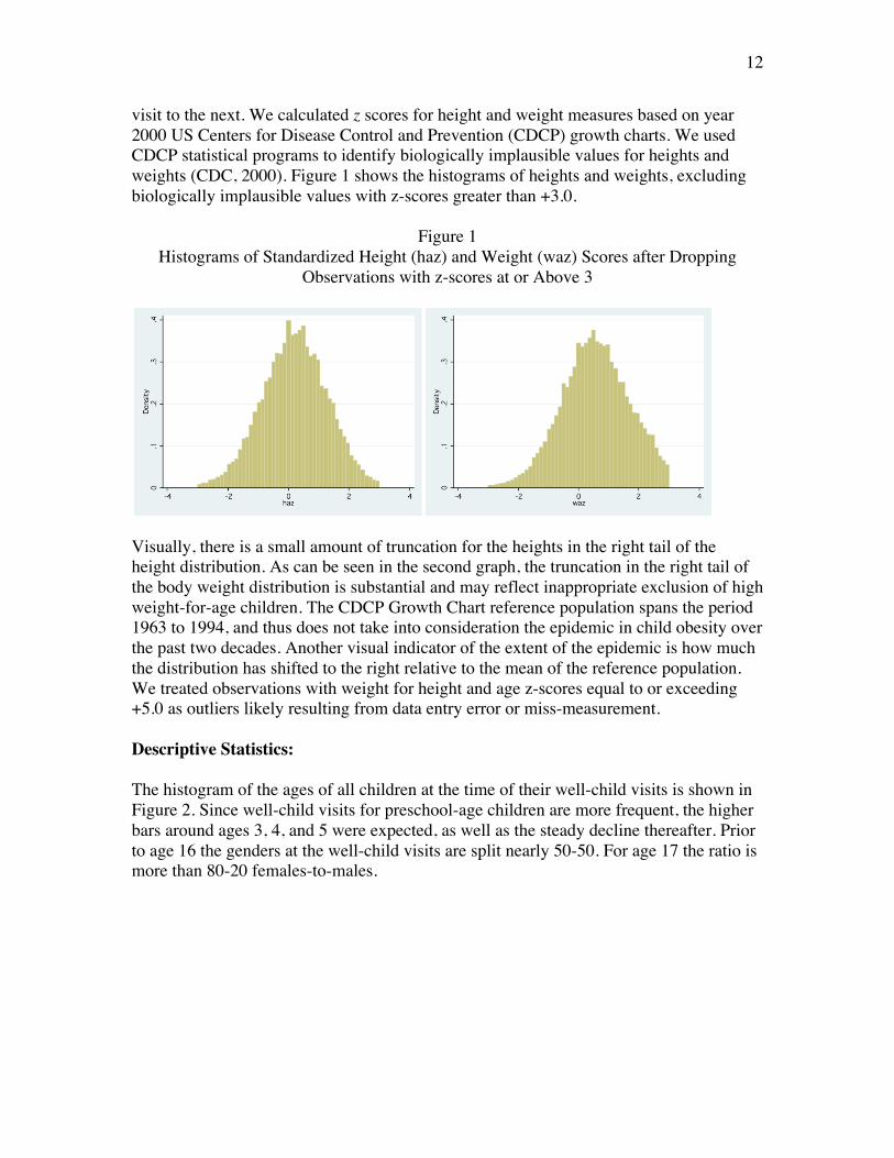
visit to the next. We calculated z scores for height and weight measures based on year 2000 US Centers for Disease Control and Prevention (CDCP) growth charts. We used CDCP statistical programs to identify biologically implausible values for heights and weights (CDC, 2000). Figure 1 shows the histograms of heights and weights, excluding biologically implausible values with z-scores greater than +3.0.

Figure 1 Histograms of Standardized Height (haz) and Weight (waz) Scores after Dropping

Observations with z-scores at or Above 3

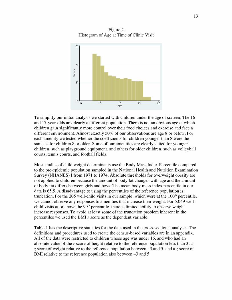
Visually, there is a small amount of truncation for the heights in the right tail of the height distribution. As can be seen in the second graph, the truncation in the right tail of the body weight distribution is substantial and may reflect inappropriate exclusion of high weight-for-age children. The CDCP Growth Chart reference population spans the period 1963 to 1994, and thus does not take into consideration the epidemic in child obesity over the past two decades. Another visual indicator of the extent of the epidemic is how much the distribution has shifted to the right relative to the mean of the reference population. We treated observations with weight for height and age z-scores equal to or exceeding +5.0 as outliers likely resulting from data entry error or miss-measurement. Descriptive Statistics: The histogram of the ages of all children at the time of their well-child visits is shown in Figure 2. Since well-child visits for preschool-age children are more frequent, the higher bars around ages 3, 4, and 5 were expected, as well as the steady decline thereafter. Prior to age 16 the genders at the well-child visits are split nearly 50-50. For age 17 the ratio is more than 80-20 females-to-males.

13

Figure 2 Histogram of Age at Time of Clinic Visit

To simplify our initial analysis we started with children under the age of sixteen. The 16- and 17-year-olds are clearly a different population. There is not an obvious age at which children gain significantly more control over their food choices and exercise and face a different environment. Almost exactly 50% of our observations are age 8 or below. For each amenity we tested whether the coefficients for children younger than 8 were the same as for children 8 or older. Some of our amenities are clearly suited for younger children, such as playground equipment, and others for older children, such as volleyball courts, tennis courts, and football fields. Most studies of child weight determinants use the Body Mass Index Percentile compared to the pre-epidemic population sampled in the National Health and Nutrition Examination Survey (NHANES) I from 1971 to 1974. Absolute thresholds for overweight obesity are not applied to children because the amount of body fat changes with age and the amount of body fat differs between girls and boys. The mean body mass index percentile in our data is 65.5. A disadvantage to using the percentiles of the reference population is truncation. For the 205 well-child visits in our sample, which were at the 100th percentile, we cannot observe any responses to amenities that increase their weight. For 5,049 well-child visits at or above the 99th percentile, there is limited ability to observe weight increase responses. To avoid at least some of the truncation problem inherent in the percentiles we used the BMI z score as the dependent variable.

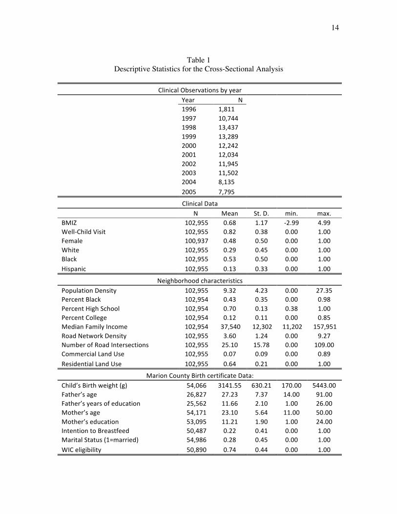
Table 1 has the descriptive statistics for the data used in the cross-sectional analysis. The definitions and procedures used to create the census-based variables are in an appendix. All of the data were restricted to children whose age was under 16, and who had an absolute value of the z score of height relative to the reference population less than 3, a z score of weight relative to the reference population between –3 and 5, and a z score of BMI relative to the reference population also between –3 and 5

14

Table 1

Descriptive Statistics for the Cross-Sectional Analysis

ClinicalObservationsbyyear Year N 1996 1,811 1997 10,744 1998 13,437 1999 13,289 2000 12,242 2001 12,034 2002 11,945 2003 11,502 2004 8,135 2005 7,795

ClinicalData N Mean St.D. min. max.BMIZ 102,955 0.68 1.17 ‐2.99 4.99Well‐ChildVisit 102,955 0.82 0.38 0.00 1.00Female 100,937 0.48 0.50 0.00 1.00White 102,955 0.29 0.45 0.00 1.00Black 102,955 0.53 0.50 0.00 1.00Hispanic 102,955 0.13 0.33 0.00 1.00

NeighborhoodcharacteristicsPopulationDensity 102,955 9.32 4.23 0.00 27.35PercentBlack 102,954 0.43 0.35 0.00 0.98PercentHighSchool 102,954 0.70 0.13 0.38 1.00PercentCollege 102,954 0.12 0.11 0.00 0.85MedianFamilyIncome 102,954 37,540 12,302 11,202 157,951RoadNetworkDensity 102,955 3.60 1.24 0.00 9.27NumberofRoadIntersections 102,955 25.10 15.78 0.00 109.00CommercialLandUse 102,955 0.07 0.09 0.00 0.89ResidentialLandUse 102,955 0.64 0.21 0.00 1.00

MarionCountyBirthcertificateData:Child’sBirthweight(g) 54,066 3141.55 630.21 170.00 5443.00Father’sage 26,827 27.23 7.37 14.00 91.00Father’syearsofeducation 25,562 11.66 2.10 1.00 26.00Mother’sage 54,171 23.10 5.64 11.00 50.00Mother’seducation 53,095 11.21 1.90 1.00 24.00IntentiontoBreastfeed 50,487 0.22 0.41 0.00 1.00MaritalStatus(1=married) 54,986 0.28 0.45 0.00 1.00WICeligibility 50,890 0.74 0.44 0.00 1.00

15

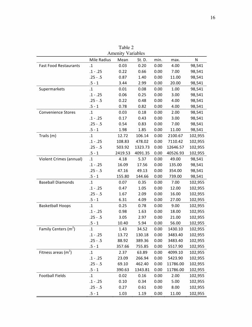
Table 2 has the environmental variables that are based on the annual Marion County food establishment inspections, Indianapolis Department of Parks and Recreation records, the Indianapolis and Marion County crime reports, and on our photo interpretation of recreational amenities. These are reported within buffers of 0.1 mile, 0.1 to 0.25 miles, 0.25 to 0.5 miles, and within 1 mile. The table reports the average values by buffer over the study period.

16

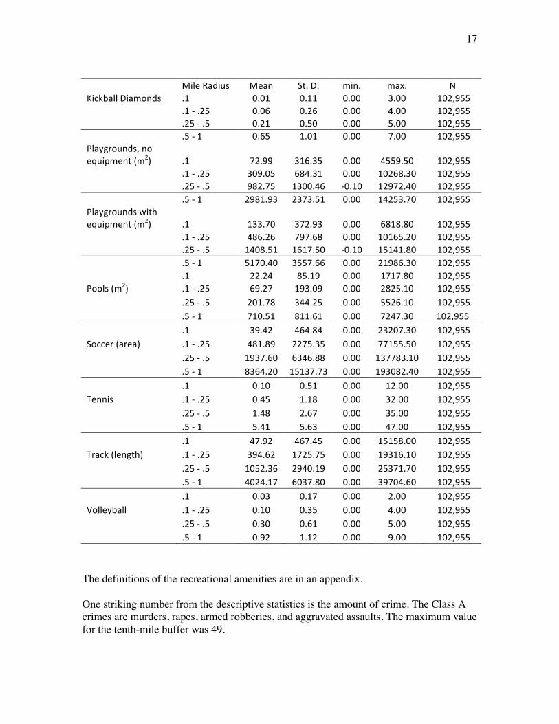
Table 2 Amenity Variables

MileRadius Mean St.D. min. max. NFastFoodRestaurants .1 0.03 0.20 0.00 4.00 98,541 .1‐.25 0.22 0.66 0.00 7.00 98,541 .25‐.5 0.87 1.40 0.00 11.00 98,541 .5‐1 3.44 2.99 0.00 20.00 98,541Supermarkets .1 0.01 0.08 0.00 1.00 98,541 .1‐.25 0.06 0.25 0.00 3.00 98,541 .25‐.5 0.22 0.48 0.00 4.00 98,541 .5‐1 0.78 0.82 0.00 4.00 98,541ConvenienceStores .1 0.03 0.18 0.00 2.00 98,541 .1‐.25 0.17 0.43 0.00 3.00 98,541 .25‐.5 0.54 0.83 0.00 7.00 98,541 .5‐1 1.98 1.85 0.00 11.00 98,541Trails(m) .1 12.72 106.14 0.00 2100.67 102,955 .1‐.25 108.83 478.02 0.00 7110.42 102,955 .25‐.5 503.92 1323.73 0.00 12646.57 102,955 .5‐1 2419.53 4091.35 0.00 40526.93 102,955ViolentCrimes(annual) .1 4.18 5.37 0.00 49.00 98,541 .1‐.25 16.09 17.56 0.00 135.00 98,541 .25‐.5 47.16 49.13 0.00 354.00 98,541 .5‐1 155.80 144.66 0.00 739.00 98,541BaseballDiamonds .1 0.07 0.35 0.00 7.00 102,955 .1‐.25 0.47 1.05 0.00 12.00 102,955 .25‐.5 1.67 2.09 0.00 16.00 102,955 .5‐1 6.31 4.09 0.00 27.00 102,955BasketballHoops .1 0.25 0.78 0.00 9.00 102,955 .1‐.25 0.98 1.63 0.00 18.00 102,955 .25‐.5 3.05 2.97 0.00 21.00 102,955 .5‐1 10.40 5.94 0.00 56.00 102,955FamilyCenters(m2) .1 1.43 34.52 0.00 1430.10 102,955 .1‐.25 13.72 130.18 0.00 3483.40 102,955 .25‐.5 88.92 389.36 0.00 3483.40 102,955 .5‐1 357.66 755.85 0.00 5517.90 102,955Fitnessareas(m2) .1 2.37 63.89 0.00 4099.10 102,955 .1‐.25 23.09 266.94 0.00 5423.90 102,955 .25‐.5 69.10 462.40 0.00 11786.00 102,955 .5‐1 390.63 1343.81 0.00 11786.00 102,955FootballFields .1 0.02 0.16 0.00 2.00 102,955 .1‐.25 0.10 0.34 0.00 5.00 102,955 .25‐.5 0.27 0.61 0.00 8.00 102,955 .5‐1 1.03 1.19 0.00 11.00 102,955

17

MileRadius Mean St.D. min. max. NKickballDiamonds .1 0.01 0.11 0.00 3.00 102,955 .1‐.25 0.06 0.26 0.00 4.00 102,955 .25‐.5 0.21 0.50 0.00 5.00 102,955 .5‐1 0.65 1.01 0.00 7.00 102,955Playgrounds,noequipment(m2) .1 72.99 316.35 0.00 4559.50 102,955 .1‐.25 309.05 684.31 0.00 10268.30 102,955 .25‐.5 982.75 1300.46 ‐0.10 12972.40 102,955 .5‐1 2981.93 2373.51 0.00 14253.70 102,955Playgroundswithequipment(m2) .1 133.70 372.93 0.00 6818.80 102,955 .1‐.25 486.26 797.68 0.00 10165.20 102,955 .25‐.5 1408.51 1617.50 ‐0.10 15141.80 102,955 .5‐1 5170.40 3557.66 0.00 21986.30 102,955 .1 22.24 85.19 0.00 1717.80 102,955Pools(m2) .1‐.25 69.27 193.09 0.00 2825.10 102,955 .25‐.5 201.78 344.25 0.00 5526.10 102,955 .5‐1 710.51 811.61 0.00 7247.30 102,955 .1 39.42 464.84 0.00 23207.30 102,955Soccer(area) .1‐.25 481.89 2275.35 0.00 77155.50 102,955 .25‐.5 1937.60 6346.88 0.00 137783.10 102,955 .5‐1 8364.20 15137.73 0.00 193082.40 102,955

.1 0.10 0.51 0.00 12.00 102,955Tennis .1‐.25 0.45 1.18 0.00 32.00 102,955 .25‐.5 1.48 2.67 0.00 35.00 102,955 .5‐1 5.41 5.63 0.00 47.00 102,955

.1 47.92 467.45 0.00 15158.00 102,955Track(length) .1‐.25 394.62 1725.75 0.00 19316.10 102,955 .25‐.5 1052.36 2940.19 0.00 25371.70 102,955 .5‐1 4024.17 6037.80 0.00 39704.60 102,955

.1 0.03 0.17 0.00 2.00 102,955Volleyball .1‐.25 0.10 0.35 0.00 4.00 102,955 .25‐.5 0.30 0.61 0.00 5.00 102,955 .5‐1 0.92 1.12 0.00 9.00 102,955

The definitions of the recreational amenities are in an appendix. One striking number from the descriptive statistics is the amount of crime. The Class A crimes are murders, rapes, armed robberies, and aggravated assaults. The maximum value for the tenth-mile buffer was 49.

18

Estimation Strategy: Our initial data set consists of fixed information on the child (race, sex, family composition at birth), changing information on the child (height, weight, and age at each clinic visit), fixed information on the parents (race, mother’s and possibly father’s education at the child’s birth), changing information on the family (residence), the built environment near the residence at the time of each clinic visit, crime counts by year within buffers around the child’s home, and some socio-economic information (at the level of the block group), and road network data. As was mentioned above, to control for the normal variations in BMI as the child ages we use age-sex adjusted base-period BMI z scores as the dependent variable. We estimate two main types of models, OLS and Fixed Effects for a child at a stable address across serial clinic visits. The key identifying assumption is that households that stay at the same location after an amenity is placed near their residence retain the same preferences they had before the amenity was added. Under this assumption the household fixed effect would remove constant-over-time preferences for location amenities and any other unobserved variables that did not change for each household. For example, the parents’ discount rate over future consumption by either themselves or their children and their altruism toward their children would wash out in the fixed effects specification. What are the potential criticisms of this estimation strategy? People might move, or more generally they might change preferences, in response to changes in their child’s overweight status, in which case the FE design would not remove the bias. We doubt that preferences change rapidly. Moreover, we can observe households that did and did not move after a change in child overweight status. We can compare the movers and stayers, and also compare households that are closer and further from the changed amenity. Another potential criticism is that there are unobserved variables common to households that are located near the new amenity. If the households in a neighborhood lobbied the Parks Department to obtain the playground or pool built near them, then there would be some common-to-the-neighborhood but unobserved-to-the-econometrician interest in exercise that would bias the estimates. A pool placed near a neighborhood where the parents had not lobbied (presumably because they were anxious to have their children use the new pool) would have a smaller effect on child overweight. This is the endogeneity problem in another guise. More problematic is the location of privately-owned amenities such as fast food restaurants or supermarkets. These types of firms often employ market researchers to identify areas where households will be the most receptive to a fast food outlet or the most likely to buy fresh produce. We can use robust estimators that yield consistent estimates of the standard errors when there are common-but-unobserved differences at a neighborhood level but without the original information that was in the hands of the

19

market researchers, we cannot fully control for differences among households in receptiveness to fast food or fresh produce. At least the direction of any potential bias is clear. We will have upper-bound estimates on child overweight effect of these privately-owned amenities. Thus, if any of them turn out to have a negligible estimated effect, we can be confident that public policy aimed at increasing or reducing these amenities would have no impact. Further, by looking at the trends in BMI z score (bmiz) before amenities such as fast food arrived, we can test whether the children who will gain an amenity in the future differed from those who will not. Another issue that we will have to address in future studies is continuing effects of a given change. Our FE model shows the impact for children of a given age of an increase or decrease in an amenity on bmiz from one well-child visit to the next. The exact exposure to the changed amenity is not known, even though the dates of the well-child visits are exact, because the food inspections and aerial photographs are updated annually.

20

Results: To see how much of the variation in bmiz can be accounted for by the fixed mother and child characteristics, bmiz was regressed on all of the variables in Table 1, using robust standard errors clustered on the child’s ID. Only the significant variables are listed. Three of the year-indicator variables were significant at the 10% level but these are omitted as well. The results are also reported separately for children under age 8 and over age 8. Age is measured at the time of the clinic visit and is a continuous variable.

Table 3 OLS Regression of Fixed Mother and Child Characteristics

Variable AllAges Age<8 Age>8Age 0.098** 0.218** 0.220** (0.013) (0.046) (0.062)AgeSquared ‐0.003** ‐0.014** ‐0.008** (0.001) (0.004) (0.003)Well‐ChildVisit ‐0.052+ ‐0.035 ‐0.074+ (0.029) (0.038) (0.040)Female 0.027 ‐0.050+ 0.140** (0.026) (0.028) (0.039)White ‐0.155* ‐0.125+ ‐0.156 (0.063) (0.067) (0.116)Black ‐0.066 ‐0.083 ‐0.034 (0.063) (0.069) (0.116)Hispanic 0.356** 0.336** 0.251 (0.087) (0.095) (0.168)AgeofMother 0.009** 0.008** 0.012** (0.003) (0.003) (0.004)BirthWeight(1000g) 0.379** 0.434** 0.293** (0.022) (0.025) (0.033)Mother’sEducation ‐0.015+ ‐0.025** 0.003 (0.008) (0.009) (0.013)ProportionBlack ‐0.146** ‐0.226** ‐0.021 (0.047) (0.055) (0.071)ProportionwithCollege 0.268 0.340+ 0.148 (0.173) (0.194) (0.267)FamilyIncome ‐0.000* ‐0.000+ ‐0.000+ (0.000) (0.000) (0.000)Constant ‐0.890** ‐1.271** ‐1.581** (0.185) (0.255) (0.430)Observations 42890 25436 17420R‐squared 0.07 0.08 0.05

Robuststandarderrorsinparentheses +significantat10%;*significantat5%;**significantat1%

21

About 7.4% of the overall variation in bmiz can be accounted for by fixed child characteristics, mother’s characteristics, and neighborhood characteristics as of the 2000 census. The explanatory power is 8% for the younger children and 5% for the older children. The increased explanatory power of the model for younger children may be attributable to the birth certificate data more accurately representing the current socioeconomic environment of the study subject. The sign on the well-child visit indicator is negative and significant overall and for the older children. The negative association between child weight and well-child care is counter-intuitive. The well-child variable, in theory, represents the health status of the child, with poorer health status children having systematically lower body mass index. Recall that visits with diagnostic codes known to affect body weight were dropped from the dataset (pregnancy, endocrine disorders, cancer, congenital heart disease, chromosomal disorders, and metabolic disorders). The well-child variable may reflect behavior practices of the child’s caregivers. Caregivers who less frequently access routine health maintenance for their children, or primarily bring their children in for sick-child visits, may be less supportive of child health behaviors associated with optimal child weight (e.g. promoting routine physical activity or a nutritious diet). This behavioral interpretation is supported by a HMO study that found that overweight children were less likely to have well child visits (Estabrooks and Shetterly, 2007).

Interestingly, over a 3-year period, overweight children show significantly fewer well-child visits. This could indicate that overweight children receive well-child visit care during sick visits that occur at a time that is proximal to a future well-child visit. It could also indicate that parents of overweight children feel that well-care visits are not necessary as a result of a higher frequency of sick visits. Finally, it could also indicate that overweight children avoid well-care visits as a method to avoid receiving advice about their weight. (p. 226)

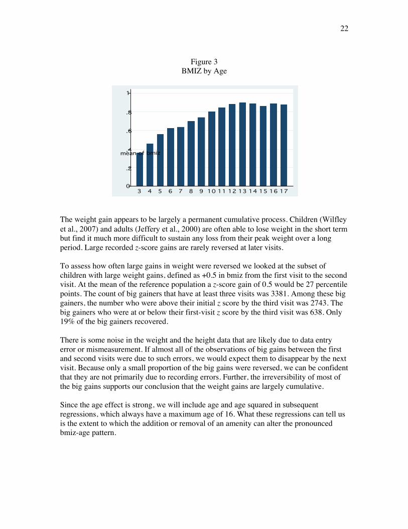
To foreshadow some of our fixed effects results, the sign of well-child visit indicator is reversed and the coefficient is significant. Thus, for a given child, a sick-child visit is associated with lower weight. Relative to the reference population, bmiz is increasing rapidly with age. As children age from the sample minimum of 3 to the maximum of 16 years their predicted bmiz increases by 0.6. The mean bmiz scores for children in the age range 3 to under 4 is 0.43, while for children in the age range 15 to under 16 it is 0.85. The age and age squared specification is convenient, but a histogram suggests a rapid increase up to age 13, and level bmiz thereafter.

22

Figure 3

BMIZ by Age

The weight gain appears to be largely a permanent cumulative process. Children (Wilfley et al., 2007) and adults (Jeffery et al., 2000) are often able to lose weight in the short term but find it much more difficult to sustain any loss from their peak weight over a long period. Large recorded z-score gains are rarely reversed at later visits. To assess how often large gains in weight were reversed we looked at the subset of children with large weight gains, defined as +0.5 in bmiz from the first visit to the second visit. At the mean of the reference population a z-score gain of 0.5 would be 27 percentile points. The count of big gainers that have at least three visits was 3381. Among these big gainers, the number who were above their initial z score by the third visit was 2743. The big gainers who were at or below their first-visit z score by the third visit was 638. Only 19% of the big gainers recovered. There is some noise in the weight and the height data that are likely due to data entry error or mismeasurement. If almost all of the observations of big gains between the first and second visits were due to such errors, we would expect them to disappear by the next visit. Because only a small proportion of the big gains were reversed, we can be confident that they are not primarily due to recording errors. Further, the irreversibility of most of the big gains supports our conclusion that the weight gains are largely cumulative. Since the age effect is strong, we will include age and age squared in subsequent regressions, which always have a maximum age of 16. What these regressions can tell us is the extent to which the addition or removal of an amenity can alter the pronounced bmiz-age pattern.

0

.2

.4

.6

.8

1

mean of bmiz

3 4 5 6 7 8 9 10 11 12 13 14 15 16 17

23

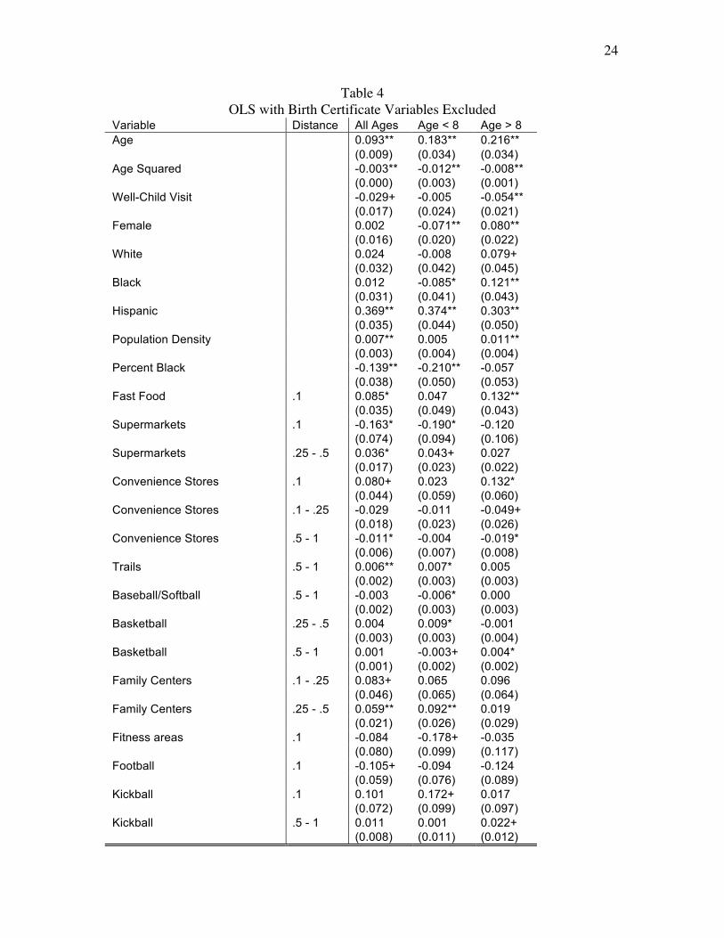
The birth certificate variables reduce the possible sample size by two-thirds. What happens to the amenity variables if birth certificate variables are dropped and the sample size expands? With 36,849 children and 96,522 clinic visits, 12 of the recreational amenities are significant at the 10% level, compared to 7 with the 41,849 visits by 13,027 children. These results are in Table 4.

24

Table 4 OLS with Birth Certificate Variables Excluded

Variable Distance All Ages Age < 8 Age > 8 Age 0.093** 0.183** 0.216** (0.009) (0.034) (0.034) Age Squared -0.003** -0.012** -0.008** (0.000) (0.003) (0.001) Well-Child Visit -0.029+ -0.005 -0.054** (0.017) (0.024) (0.021) Female 0.002 -0.071** 0.080** (0.016) (0.020) (0.022) White 0.024 -0.008 0.079+ (0.032) (0.042) (0.045) Black 0.012 -0.085* 0.121** (0.031) (0.041) (0.043) Hispanic 0.369** 0.374** 0.303** (0.035) (0.044) (0.050) Population Density 0.007** 0.005 0.011** (0.003) (0.004) (0.004) Percent Black -0.139** -0.210** -0.057 (0.038) (0.050) (0.053) Fast Food .1 0.085* 0.047 0.132** (0.035) (0.049) (0.043) Supermarkets .1 -0.163* -0.190* -0.120 (0.074) (0.094) (0.106) Supermarkets .25 - .5 0.036* 0.043+ 0.027 (0.017) (0.023) (0.022) Convenience Stores .1 0.080+ 0.023 0.132* (0.044) (0.059) (0.060) Convenience Stores .1 - .25 -0.029 -0.011 -0.049+ (0.018) (0.023) (0.026) Convenience Stores .5 - 1 -0.011* -0.004 -0.019* (0.006) (0.007) (0.008) Trails .5 - 1 0.006** 0.007* 0.005 (0.002) (0.003) (0.003) Baseball/Softball .5 - 1 -0.003 -0.006* 0.000 (0.002) (0.003) (0.003) Basketball .25 - .5 0.004 0.009* -0.001 (0.003) (0.003) (0.004) Basketball .5 - 1 0.001 -0.003+ 0.004* (0.001) (0.002) (0.002) Family Centers .1 - .25 0.083+ 0.065 0.096 (0.046) (0.065) (0.064) Family Centers .25 - .5 0.059** 0.092** 0.019 (0.021) (0.026) (0.029) Fitness areas .1 -0.084 -0.178+ -0.035 (0.080) (0.099) (0.117) Football .1 -0.105+ -0.094 -0.124 (0.059) (0.076) (0.089) Kickball .1 0.101 0.172+ 0.017 (0.072) (0.099) (0.097) Kickball .5 - 1 0.011 0.001 0.022+ (0.008) (0.011) (0.012)

25

Variable Distance All Ages Age < 8 Age > 8 Playgrounds, no equipment .5 - 1 -0.003 0.004 -0.010+ (0.004) (0.005) (0.005) Playgrounds, with equipment .5 - 1 -0.003 0.001 -0.007* (0.002) (0.003) (0.003) Track and field .1 0.031+ 0.008 0.080** (0.019) (0.023) (0.026) Volleyball .1 0.078* 0.106* 0.040 (0.038) (0.044) (0.063) Volleyball .25 - .5 0.021+ 0.011 0.025 (0.012) (0.015) (0.017) Volleyball .5 - 1 0.007 -0.004 0.018+ (0.007) (0.009) (0.010) Constant 0.181+ 0.007 -0.557* (0.106) (0.158) (0.237) Observations 96522 50503 45951 R-squared 0.04 0.04 0.02 Robust standard errors in parentheses + significant at 10%; * significant at 5%; ** significant at 1%

The recreational amenities that are significant are at various distances. There is no reason to expect any real effects of different amenities to operate over the same distance in all cases. Also, in the smaller rings there may be real effects but too few observations to yield statistically significant results. Some of the signs of the significant amenities are conventional, e.g. fast food within a tenth mile is associated with a higher bmiz, while supermarkets within a tenth mile are associated with lower bmiz. Very few of the recreational amenities have a significant negative sign. These include baseball for children under age 8 at 0.5 to 1 mile, fitness areas for younger children at 0.1 miles, football for the combined age groups, and playgrounds without equipment at the 0.5 to 1 for the over age 8 children. The problem with the OLS results is that they have little explanatory power, most of the demographic variables have limited policy implications, and most importantly, it is impossible to know if the associations are causal. For example, track and field facilities and football fields are almost all located at middle schools and high schools. Are the bmiz differences associated with these variables due to children using these amenities or simply to unobserved differences in the families that chose to live near these schools? The fast food restaurants, supermarkets and even convenience stores are located on major roads. Are the bmiz associations of these amenities due to proximity to these food sources or to unobservable differences in households living near major roads?

26

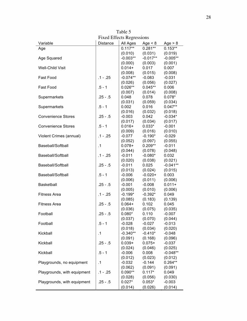
The endogeneity question for fast-food effects on adults living in rural areas was addressed in a very recent working paper (Anderson and Matsa, 2008), which used location near an interstate highway exit as an instrument for fast food location. Highway exits have fast food restaurants to serve travelers; they provide more fast food outlets than would otherwise be supported by small communities. The paper relies on self-reported weights and is limited to adults. The conclusion is that fast food has no causal effect on adult BMI. Fixed Effects Regressions: In the FE regressions below, we dropped all variables that are constant at the level of the child. Again, this sample is restricted to observations in which a child remains at the same address between clinic visits. The same restrictions on age and biologically-implausible values of bmiz, height, and weight are also applied. The covariates to the environmental/amenity variables are age and age squared, year of clinic visit indicator variables, an indicator for a well-child visit, and crime at the four rings. Crime was never significant in the OLS regressions at any circle size. In cross section, at least, a direct effect of crime on bmiz was not observed. Again, the coefficients on the year dummy variables are not reported, and all non-significant coefficients are not reported. As was mentioned, the well-child variable is now positive and significant at the 10% level for all children. In terms of the number of amenities with significant coefficients, there are 40, compared to the 30 in the OLS regression model. In addition to having a different count of amenities with significant coefficients, there are very few overlaps of the same amenity being significant at the same distance. Adding a fast food restaurant within a quarter mile of the same child appears to significantly reduce the child’s bmiz. Recall that in the cross-sectional results at the tenth mile buffer the association between bmiz and fast food was positive. From a public policy perspective the FE results for the recreational amenities are somewhat discouraging. The ones with negative and significant coefficients are baseball at a 0.1 to 0.25 miles at a 5% level, baseball over age 8 at 0.25 to 0.5 miles at a 1% level, baseball under age 8 at the 0.5 to 1.0 mile at a 10% level, fitness areas for all ages and children under 8 at the 0.1 to 0.25 mile, kickball overall and for under 8 at the 0.1 mile at 1% and 5% respectively, kickball at the 1 mile for children over 8 at a 1% level, tennis for children over 8 from 0.1 to 0.25 miles at a 1% level, volleyball for children over 8 at a 1% level, and volleyball overall and for children under 8 at 0.5 to a 1 mile at 5% and 10% level respectively. If the reported results were causal effects, then bmiz-reducing policy would be to build fast food restaurants within a quarter mile of the child’s home and surround them with a fitness area and a kickball diamond. Before much credence can be given to these estimates, the issue of the endogeneity of the placement of these amenities must be addressed.

27

The FE framework allows for separate consideration of gains and losses in amenities. We tested whether the coefficient on a gain was the same as for a loss for every amenity and could not reject the null hypothesis of equality in a single case. Also, we looked at assumption of linearity of effects, e.g. that a gain from 0 to 1 is the same as a gain from 1 to 2. A very high fraction of all of the changes we observed in counts of amenities are in the range of 0 to 1 or from 1 to 0. We could not reject the null hypothesis of linearity largely because we observed too few higher-order changes.

28

Table 5 Fixed Effects Regressions

Variable Distance All Ages Age < 8 Age > 8 Age 0.117** 0.281** 0.153** (0.010) (0.031) (0.019) Age Squared -0.003** -0.017** -0.005** (0.000) (0.003) (0.001) Well-Child Visit 0.014+ 0.017 0.007 (0.008) (0.015) (0.008) Fast Food .1 - .25 -0.074** -0.083 -0.031 (0.026) (0.056) (0.027) Fast Food .5 - 1 0.026** 0.045** 0.006 (0.007) (0.014) (0.008) Supermarkets .25 - .5 0.048 0.078 0.078* (0.031) (0.059) (0.034) Supermarkets .5 - 1 0.002 0.016 0.047** (0.016) (0.032) (0.018) Convenience Stores .25 - .5 -0.003 0.042 -0.034* (0.017) (0.034) (0.017) Convenience Stores .5 - 1 0.016+ 0.033* -0.001 (0.009) (0.016) (0.010) Violent Crimes (annual) .1 - .25 -0.077 -0.190* -0.029 (0.052) (0.097) (0.055) Baseball/Softball .1 0.078+ 0.209** -0.011 (0.044) (0.078) (0.048) Baseball/Softball .1 - .25 -0.011 -0.080* 0.032 (0.020) (0.038) (0.021) Baseball/Softball .25 - .5 -0.011 0.025 -0.041** (0.013) (0.024) (0.015) Baseball/Softball .5 - 1 -0.006 -0.020+ 0.003 (0.006) (0.011) (0.006) Basketball .25 - .5 -0.001 -0.008 0.011+ (0.005) (0.010) (0.006) Fitness Area .1 - .25 -0.199* -0.392* 0.049 (0.085) (0.183) (0.139) Fitness Area .25 - .5 0.064+ 0.102 0.045 (0.036) (0.075) (0.035) Football .25 - .5 0.080* 0.110 -0.007 (0.037) (0.070) (0.044) Football .5 - 1 -0.028 -0.027 -0.013 (0.018) (0.034) (0.020) Kickball .1 -0.340** -0.410* -0.048 (0.091) (0.168) (0.096) Kickball .25 - .5 0.039+ 0.075+ -0.037 (0.024) (0.046) (0.025) Kickball .5 - 1 -0.006 0.008 -0.048** (0.012) (0.023) (0.012) Playgrounds, no equipment .1 -0.032 -0.144 0.264** (0.062) (0.091) (0.091) Playgrounds, with equipment .1 - .25 0.090** 0.117* 0.049 (0.028) (0.056) (0.030) Playgrounds, with equipment .25 - .5 0.027* 0.053* -0.003 (0.014) (0.026) (0.014)

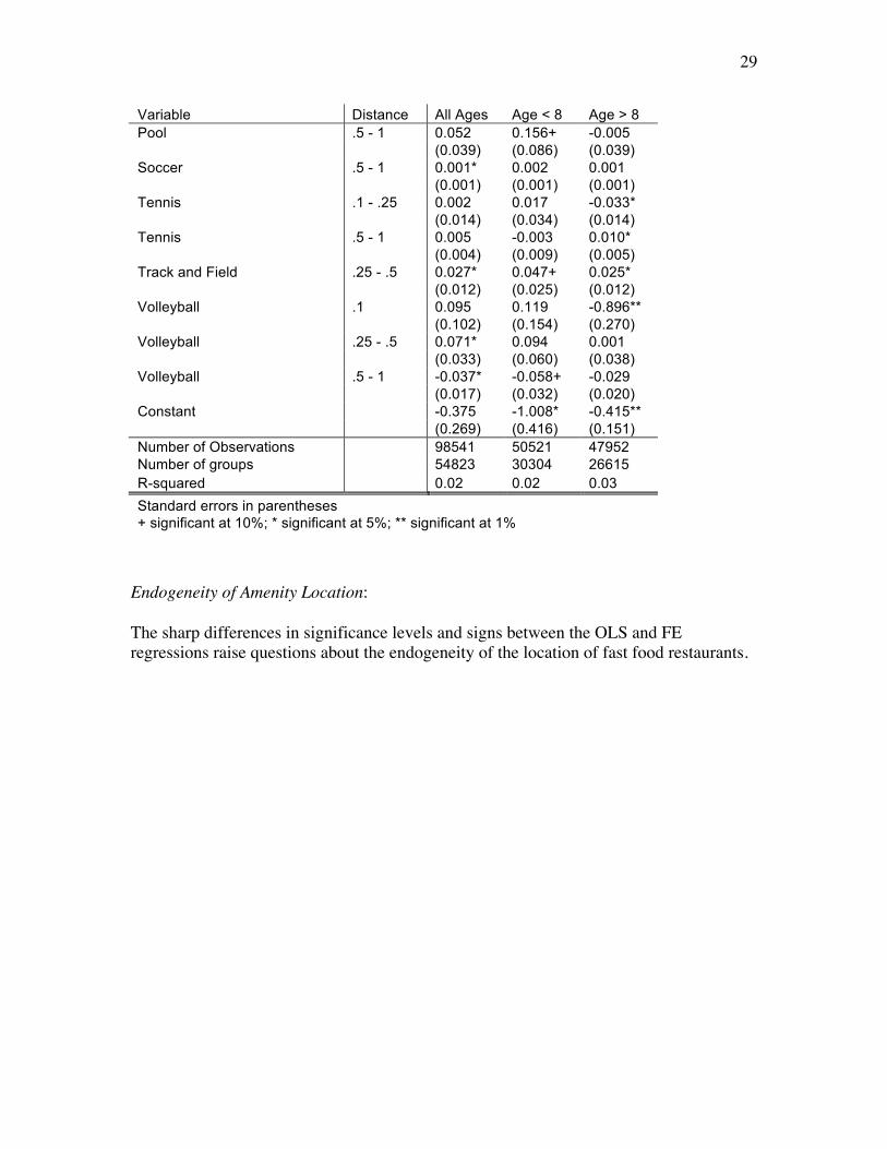
29

Variable Distance All Ages Age < 8 Age > 8 Pool .5 - 1 0.052 0.156+ -0.005 (0.039) (0.086) (0.039) Soccer .5 - 1 0.001* 0.002 0.001 (0.001) (0.001) (0.001) Tennis .1 - .25 0.002 0.017 -0.033* (0.014) (0.034) (0.014) Tennis .5 - 1 0.005 -0.003 0.010* (0.004) (0.009) (0.005) Track and Field .25 - .5 0.027* 0.047+ 0.025* (0.012) (0.025) (0.012) Volleyball .1 0.095 0.119 -0.896** (0.102) (0.154) (0.270) Volleyball .25 - .5 0.071* 0.094 0.001 (0.033) (0.060) (0.038) Volleyball .5 - 1 -0.037* -0.058+ -0.029 (0.017) (0.032) (0.020) Constant -0.375 -1.008* -0.415** (0.269) (0.416) (0.151) Number of Observations 98541 50521 47952 Number of groups 54823 30304 26615 R-squared 0.02 0.02 0.03 Standard errors in parentheses + significant at 10%; * significant at 5%; ** significant at 1%

Endogeneity of Amenity Location: The sharp differences in significance levels and signs between the OLS and FE regressions raise questions about the endogeneity of the location of fast food restaurants.

30

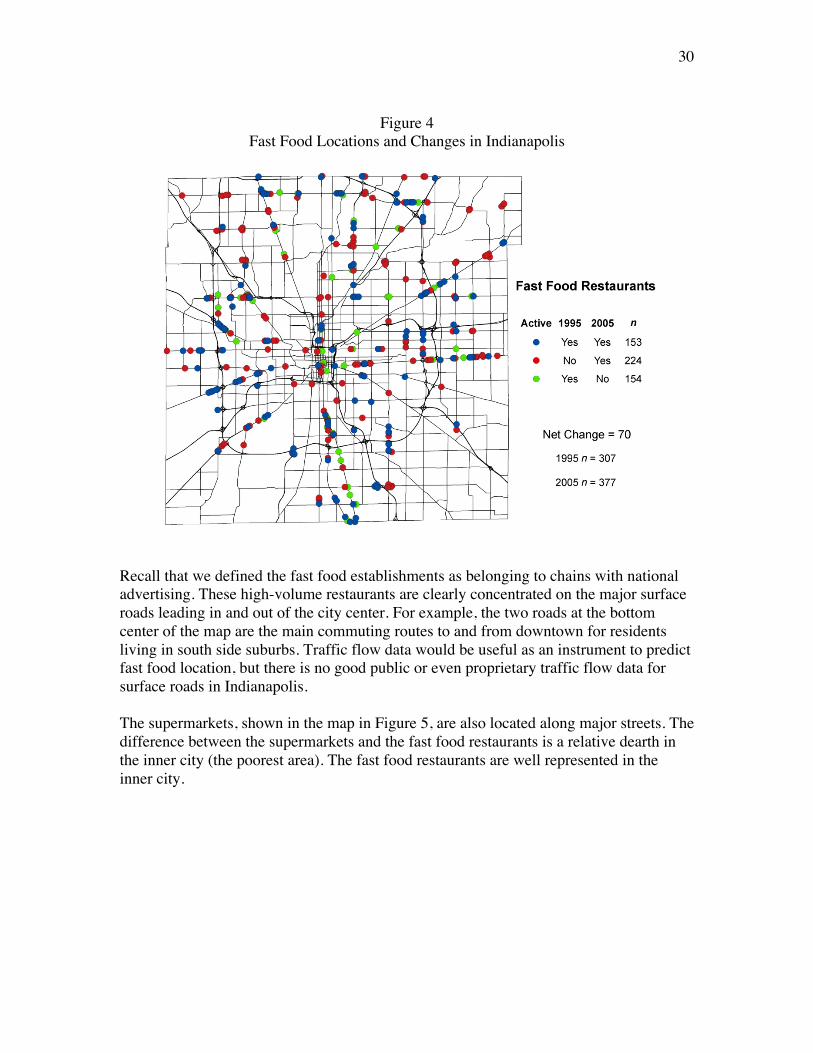
Figure 4

Fast Food Locations and Changes in Indianapolis

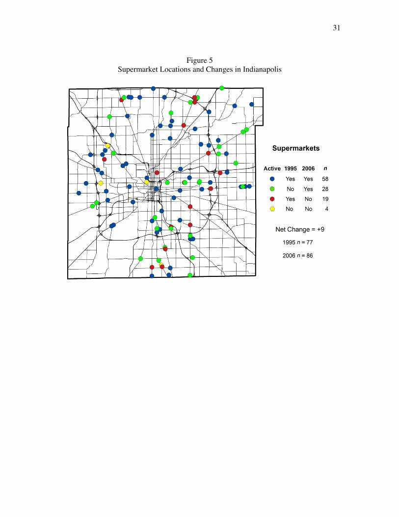
Recall that we defined the fast food establishments as belonging to chains with national advertising. These high-volume restaurants are clearly concentrated on the major surface roads leading in and out of the city center. For example, the two roads at the bottom center of the map are the main commuting routes to and from downtown for residents living in south side suburbs. Traffic flow data would be useful as an instrument to predict fast food location, but there is no good public or even proprietary traffic flow data for surface roads in Indianapolis. The supermarkets, shown in the map in Figure 5, are also located along major streets. The difference between the supermarkets and the fast food restaurants is a relative dearth in the inner city (the poorest area). The fast food restaurants are well represented in the inner city.

31

Figure 5

Supermarket Locations and Changes in Indianapolis

32

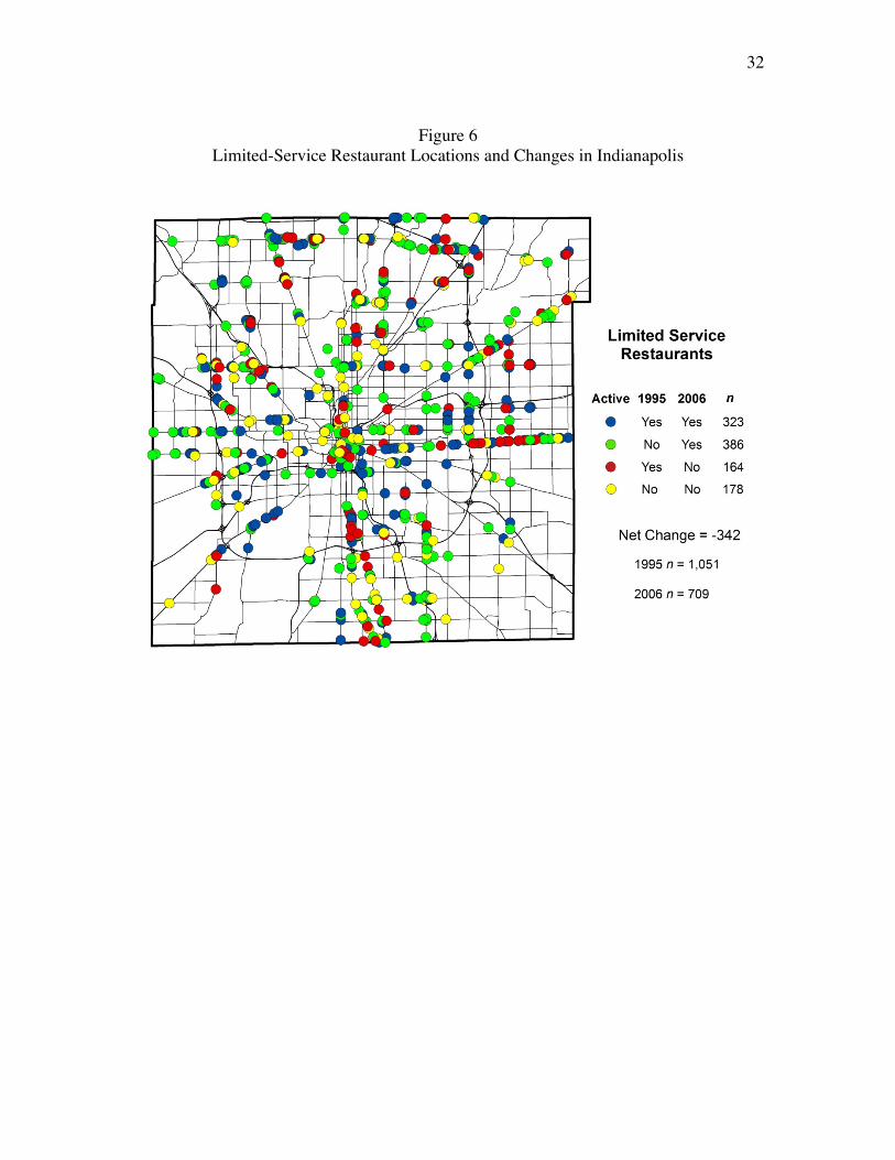
Figure 6

Limited-Service Restaurant Locations and Changes in Indianapolis

33

Figure 7

Convenience Store Locations and Changes in Indianapolis

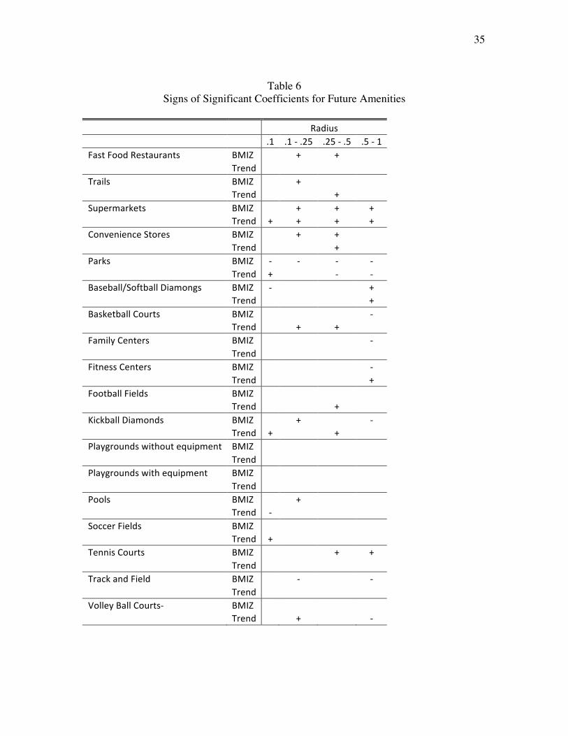
Figure 6 and 7 have the locations and changes of limited-service restaurants and convenience stores. The southwest and southeast corners of the county are still largely rural. Other than in those undeveloped areas, there are limited-service restaurants and conveniences stores widely distributed across the county. One means of addressing the endogeneity of amenity locations is to check whether the children living near future locations differed in terms of bmiz trends from the children who did not have the same type of amenity move near them. To test whether the location of new amenities is related to trends in children’s weight, we regressed children’s weight prior to the arrival of new amenities on the indicator of whether the new amenity locates next to the child in the future. We looked at differences between average z score of children’s BMI as well as differences in time trends of z scores of children’s BMI. Table 6 shows these results. The positive or negative symbol represents the sign of the coefficient on the future amenity indicator and of the interaction term of that indicator with the time trend variable provided they are significant at 5% level. The results show that only the location of supermarkets is preceded by differences in children’s weight, as well as differences in trajectories of children’s weight gain.

34

The positive trends observed at all four buffers for supermarkets undercut the claim that their new locations were selected independently of the changes in children’s bmiz. Thus, the FE results that supermarkets increase children’s weights at the half-mile buffer are suspect. Fast food restaurants appear to be entering areas with higher child bmiz values and higher rates of child obesity, at least for the quarter- and half-mile buffers. However, these initial differences in levels may not predict the change that will occur after the arrival of a new fast food restaurant. Our assumption is that gains in bmiz will be the same for a given stimulus over a broad range of initial bmiz. We believe having the same trend in bmiz for children with and without future fast food gives us an unbiased estimate of the response to the arrival of an amenity. Our negative coefficient quarter-mile fast food result with no difference in trends supports the Anderson and Matsa result cited above. While fast food meals are notoriously calorie dense, they can have no bmiz effect if children or adults offset the additional calories by eating less food at other meals or by eating fewer meals. As a means of attacking the child obesity epidemic, the Los Angeles freeze on new fast food restaurants mentioned in the introduction may be misplaced. Fast food and supermarkets are the highest-profile amenities. Of the remaining 60 trend terms (15 amenities times 4 buffers), 11 are significant. These are scattered such that none of the other amenities has a significant trend term for more than one buffer. Either the locations of these remaining amenities are not being selected on the basis of differences in bmiz trends, or we do not have enough data to detect differences in bmiz trends.

35

Table 6

Signs of Significant Coefficients for Future Amenities Radius .1 .1‐.25 .25‐.5 .5‐1FastFoodRestaurants BMIZ + + Trend Trails BMIZ + Trend + Supermarkets BMIZ + + + Trend + + + +ConvenienceStores BMIZ + + Trend + Parks BMIZ ‐ ‐ ‐ ‐ Trend + ‐ ‐Baseball/SoftballDiamongs BMIZ ‐ + Trend +BasketballCourts BMIZ ‐ Trend + + FamilyCenters BMIZ ‐ Trend FitnessCenters BMIZ ‐ Trend +FootballFields BMIZ Trend + KickballDiamonds BMIZ + ‐ Trend + + Playgroundswithoutequipment BMIZ Trend Playgroundswithequipment BMIZ Trend Pools BMIZ + Trend ‐ SoccerFields BMIZ Trend + TennisCourts BMIZ + + Trend TrackandField BMIZ ‐ ‐ Trend VolleyBallCourts‐ BMIZ Trend + ‐

36

Conclusion: The main conclusion is that cross-sectional results tell us more about who chooses to live near an amenity than what adding that amenity might do. In cross section, nearby (tenth-mile) fast food increases children’s bmiz. Our cross section regression has controls for child’s age, race, gender, mother’s age at child’s birth, mother’s education, WIC eligibility, intention to breastfeed, and many neighborhood characteristics. These are as comprehensive a set of covariates as we have seen for child BMI regressions. Other study strengths include directly measured height and weight data for a large sample size that includes high proportions of African American and Hispanic children. Still, in the fixed effects framework, nearby (quarter-mile) fast food appears to reduce children’s weights, with no difference in the trend of bmiz gain prior to the arrival of the fast food. While we doubt that fast food really reduces children’s bmiz, the results of the fixed effects models cast doubt on the highly publicized policies to reduce fast food exposure as interventions for preventing obesity. A second conclusion is that if the arrival of our amenities (other than supermarkets) is unrelated to prior trends in bmiz, then there appears to be little in the way of surefire interventions for reducing children’s bmiz, through either recreational amenities or food sellers. The best candidates appear to be baseball and softball fields, fitness areas, kickball fields, and volleyball courts. This paper began with the assertion that, at best, only one third of the child obesity epidemic has been explained. There may be some bmiz-increasing effects of adding supermarkets and convenience stores, both of which carry calorie-dense food marketed to children. The mean of the children’s bmiz in our data set is 0.6 above the bmiz of the pre-epidemic population. The sum of the coefficients for adding one supermarkets and convenience stores, at a half mile and a mile respectively, are 0.11. There is at least the potential for these food outlets to account for a substantial share of the epidemic. Public policy may need to be aimed at what children consume from supermarkets and convenience stores rather reducing the number of outlets. Our results look at the short term. They look for bmiz responses within the year the amenity arrives. It may be that a recreational amenity does have a bmiz-reducing effect on nearby children if it is measured years after its arrival. However, we have few observations with long runs of time after the arrival of an amenity.

37

Bibliography: (a) Anderson, Patricia M., Butcher, Kristin F: Reading, Writing, and Refreshments: Are School Finances Contributing to Children’s Obesity?, Journal of Human Resources, Volume 41, Number 3, Summer 2006 , pp. 467-494(28). (b) Anderson, Patricia M., Butcher, Kristin F: Childhood Obesity: Trends and Potential Causes, The Future of Children, Vol. 16, No. 1, Childhood Obesity (Spring, 2006), pp. 19-45. Anderson, Michael, Matsa, David A.: Are Restaurants Really Supersizing America?, December 30, 2007, University of California Berkeley Working Paper. Boone Janne E, Gordon-Larsen Penny, Adair Linda S, and Popkin Barry M: Screen time and physical activity during adolescence: longitudinal effects on obesity in young adulthood, International Journal of Behavioral Nutrition and Physical Activity. 2007; 4: 26. Bouchard C: Genetics of obesity: Overview and research direction. In The genetics of obesity, edited by Bouchard C, pp. 223-233. Boca Raton, 1994. Birch LL, Fisher JO: Development of eating behaviors among children and adolescents. Pediatrics 1998; 101:539-49. Bray, George A, Champagne, Catherine M: Beyond Energy Balance: There Is More to Obesity than Kilocalories, J Am Diet Assoc. 2005;105:S17-S23. Brownson RC, Baker EA, Housemann RA, et al.: Environmental and policy determinants of physical activity in the United States. Am J Public Health 2001; 91:1995-2003. Burke, Mary A, Heiland, Frank: Social Dynamics of Obesity. Economic Inquiry, vol. 45, no. 3, July 2007, pp. 571-91. Burdette HL, Whitaker RC: Neighborhood playgrounds, fast food restaurants, and crime: relationships to overweight in low-income preschool children. Preventive Medicine 2004; 38:57-63. Burdette, HL, and Whitaker, RC: A National Study of Neighborhood Safety, Outdoor Play, Television Viewing, and Obesity in Preschool Children. Pediatrics, 2005,116(3): 657-662. Cawley, John; Meyerhoefer, Chad; Newhouse, David: The Impact of State Physical Education Requirements on Youth Physical Activity and Overweight, Health Economics, vol. 16, no. 12, December 2007, pp. 1287-1301.

38

CDC, A SAS Program for the CDC Growth Charts, www.cdc.gov/nccdphp/dnpa/growthcharts/resources/sas.htm Chou S, Grossman M, Saffer H. An Economic Analysis of Adult Obesity: Results from the Behavioral Risk Factor Surveillance System NBER Working Paper #9247, National Bureau of Economic Research. Cambridge, MA, 2002. Chou, Shin-Yi, Rashad, Inas, Grossman, Michael: Fast-Food Advertising on Television and Its Influence on Childhood Obesity, NBER Working Paper No. 11879, December 2005. Clement K, Ferre P: Genetics and the pathophysiology of obesity. Pediatr Res 2003; 53:721-5. Consensus Panel: “Type 2 diabetes in children and adolescents.” American Diabetes Association, http://care.diabetesjournals.org/cgi/reprint/23/3/381.pdf. Cordain L, Miller JB, Eaton SB, et al.: Macronutrient estimations in hunter-gatherer diets. Am J Clin Nutr 2000; 72:1589-92. Corless J, Ohland G: Caught in the crosswalk: Pedestrian safety in California, 2001. Courtemanche, Charles: Working Yourself to Death? The Relationship Between Work Hours and Obesity. Working Paper, Washington University, St. Louis. (October 5, 2007) Cressie, N, Chan NH: Spatial Modeling of Regional Variables, Journal of the American Statistical Association, 1989, Vol. 84, No. 406, 393-401. Jun. Dietary Reference Intakes for Energy, Carbohydrate, Fiber, Fat, Fatty Acids, Cholesterol, Protein, and Amino Acids (Macronutrients): A Report of the Panel on Macronutrients, Subcommittees on Upper Reference Levels of Nutrients and Interpretation and Uses of Dietary Reference Intakes, and the Standing Committee on the Scientific Evaluation of Dietary Reference Intakes, 2002. DiPietro L, Mossberg HO, Stunkard AJ: A 40-year history of overweight children in Stockholm: life-time overweight, morbidity, and mortality. Int J Obes Relat Metab Disord 1994; 18:585-90 Epstein LH, Paluch RA, Gordy CC, et al.: Decreasing sedentary behaviors in treating pediatric obesity. Arch Pediatr Adolesc Med 2000; 154:220-6. Estabrooks, Paul A; Susan Shetterly: The Prevalence and Health Care Use of Overweight Children in an Integrated Health Care System. Arch Pediatr Adolesc Med. 2007;161:222-227.

39

Ewing R, Cervero R: Travel and the Built Environment: A Synthesis. Transportation Research Record 1780, 2001. Foreyt J, Goodrick K: The ultimate triumph of obesity. Lancet 1995; 346:134-5. Freedman DS, Dietz WH, Srinivasan SR, et al: The relation of overweight to cardiovascular risk factors among children and adolescents: the Bogalusa Heart Study. Pediatrics 1999; 103:1175-82. Garn SM, Clark DC: Nutrition, growth, development, and maturation: findings from the ten-state nutrition survey of 1968-1970. Pediatrics 1975; 56:306-19. Gerrior S, Bente L: Nutrient Content of the U.S. Food Supply, 1909-99: A Summary Report. U.S. Department of Agriculture, Center for Nutrition Policy and Promotion. Home Economics Research Report No. 55. 2002. Glanz K, Lankenau B, Foerster S, et al.: Environmental and policy approaches to cardiovascular disease prevention through nutrition: opportunities for state and local action. Health Educ Q 1995; 22:512-27. Gortmaker SL, Must A, Sobol AM, et al.: Television viewing as a cause of increasing obesity among children in the United States, 1986-1990. Arch Pediatr Adolesc Med 1996; 150:356-62. Gortmaker SL, Must A, Perrin JM, et al.: Social and economic consequences of overweight in adolescence and young adulthood. N Engl J Med 1993; 329:1008-12. Haas JS, Lee LB, Kaplan CP, et al.: The association of race, socioeconomic status, and health insurance status with the prevalence of overweight among children and adolescents. Am J Public Health 2003; 93:2105-10. Hedley, AA, Ogden, CL, Johnson, CL, Carroll, MD, Curtin, LR, Flegal, KM: Overweight and obesity among US children, adolescents, and adults, 1999-2002. JAMA 291:2847-50. 2004. Hill JO, Peters JC: Environmental contributions to the obesity epidemic. Science 1998; 280:1371-4. Hogan JW, Tchernis, R: Bayesian Factor Analysis for Spatially Correlated Data, with Application to Summarizing Area-Level Material Deprivation from Census Data, Journal of the American Statistical Association, Number 466, 1 June 2004 , pp. 314-324(11). HOPS, Healhier Options for Public School Children, http://agatstonresearchfoundation.org/HOPS_Study_Preliminary_Results_HOPS_1_and_HOPS_2.pdf

40

Horgen K, Choate M, Brownwell K: Television and children’s nutrition. In: Singer D, Singer J, eds. Handbook of children and the media. San Francisco: Sage, 2001:447-461. Jeffery RW: Public health strategies for obesity treatment and prevention. Am J Health Behav 2001; 25:252-9. Jeffery RW, Drewnowski A, Epstein LH; et al. Long-term maintenance of weight loss: current status. Health Psychol. 2000;19(1)(suppl):5-16. Kaushal, N: Do Food Stamps Cause Obesity? Evidence from Immigrant Experience. Journal of Health Economics, vol. 26, no. 5, September 2007, pp. 968-91. King AC, Jeffery RW, Fridinger F, et al.: Environmental and policy approaches to cardiovascular disease prevention through physical activity: issues and opportunities. Health Educ Q 1995; 22:499-511. King AC, Castro C, Wilcox S, et al.: Personal and environmental factors associated with physical inactivity among different racial-ethnic groups of U.S. middle-aged and older-aged women. Health Psychol 2000; 19:354-64. Kolata G, Thinning the Milk Does Not Mean Thinning the Child. New York Times February 12, 2006. Kortt M, Baldry J: The association between musculoskeletal disorders and obesity. Aust Health Rev 2002; 25:207-14. Kumanyika SK: Minisymposium on obesity: overview and some strategic considerations. Annu Rev Public Health 2001; 22:293-308. L.A. Times: www.latimes.com/news/local/politics/cal/la-me-fastfood30-2008jul30,0,7844906.

Life Sciences Research Office, the U.S. Department of Agriculture, Center for Nutrition Policy and Promotion, 1995, Third Report on Nutrition Monitoring in the United States Margetts B: WHO global strategy on diet, physical activity and health. Editorial. Public Health Nutr 2004; 7:361-3. Mokdad AH, Serdula MK, Dietz WH, et al.: The continuing epidemic of obesity in the United States. Jama 2000; 284:1650-1. Neff LJ, Sargent RG, McKeown RE, et al.: Black-white differences in body size perceptions and weight management practices among adolescent females. J Adolesc Health 1997; 20:459-65. Ogden CL, Flegal KM, Carroll MD, Johnson CL: Prevalence and trends in overweight among US children and adolescents, 1999-2000. JAMA 288:1728-32. 2002. Parnell K, Sargent R, Thompson SH, et al.: Black and white adolescent females’ perceptions of ideal body size. J Sch Health 1996; 66:112-8. Plantinga, Andrew J, Bernell Stephanie: The Association between Urban Sprawl and Obesity: Is It a Two-Way Street?, Journal of Regional Science, vol. 47, no. 5, December 2007, pp. 857-79. Popkin BM, Udry JR: Adolescent obesity increases significantly in second and third generation U.S. immigrants: the National Longitudinal Study of Adolescent Health. J Nutr 1998; 128:701-6. Price R: Genetics and common obesities: background, current status, strategies, and future prospects. In Handbook for obesity treatment, edited by Wadden T, Stunkard AJ, pp. 73-94. New York, NY, Guilford Press 2002. Quigley, Fran (2003), Indianapolis is missing the bus: IndyGo is worst-funded system in Midwest, Nuvo, www.nuvo.net/archive/2003/12/24/indianapolis_is_missing_the_bus.html Sallis JF, Bauman A, Pratt M: Environmental and policy interventions to promote physical activity. Am J Prev Med 1998; 15:379-97. Schadt EE, Monks SA, Drake TA, et al.: Genetics of gene expression surveyed in maize, mouse and man. Nature 2003; 422:297-302. Snyder EE, Walts B, Perusse L, et al.: The human obesity gene map: the 2003 update. Obes Res 2004; 12:369-439. Sobal J, Stunkard AJ: Socioeconomic status and obesity: a review of the literature. Psychol Bull 1989; 105:260-75.

42

Sorensen HT, Sabroe S, Rothman KJ, et al.: Relation between weight and length at birth and body mass index in young adulthood: cohort study. BMJ 1997; 315:1137. Strauss RS, Knight J: Influence of the home environment on the development of obesity in children. Pediatrics 1999; 103:e85. Strauss RS, Pollack HA: Social marginalization of overweight children. Arch Pediatr Adolesc Med 2003; 157:746-52. Tchernis, Rusty; Millimet, Daniel; Hussain, Muna: School Nutrition Programs and the Incidence of Childhood Obesity, Center for Applied Economics and Policy Research, Economics Department, Indiana University Bloomington, Caepr Working Papers: 2007-014, 2007, 37 pp. Wilfley DE, Stein RI, Saelens BE, Mockus DS, Matt GE, Hayden-Wade HA, Welch RR, Schechtman KB, Thompson PA, Epstein LH. Efficacy of maintenance treatment approaches for childhood overweight: a randomized controlled trial. JAMA. 2007 Oct 10;298(14):1661-73. Wittels EH, Thompson S: Obstructive sleep apnea and obesity. Otolaryngol Clin North Am 1990; 23:751-60.

43

Appendix on Photo Interpretation Orthorectified aerial photograph mosaics were available for most study years. The primary exception was 1996, for which no photographs of Marion County were available. Small, scattered areas were missing from the 1995 photographs. Photographs were available for 1998 for most of the county. Owing to a problem with the initial flight for 1998, no photography was available for a narrow band of the county running north to south through the center. This area was reflown in early 1999 using the same techniques; the resulting photographs were treated differently in this study from the 1998 photographs, as well as from a complete set of photographs taken later in 1999 using different techniques. The photographs varied greatly in quality; only the last four years were in color, and later years were generally of higher spatial resolution than earlier years, though the 1998 (and matching early 1999) photographs were significantly coarser than other years. Contrast was also starker and thus of lower quality in earlier years, particularly in 1995. All photographs were provided to a team of photo interpreters in digital format. In one case, 2005, images were available from Indiana University’s spatial data portal, representing the same original photography as the 2005 file photographs, but reproduced at higher resolution. Photographs were examined on computer display in ArcMap 9.2, generally at scales of 1:1000 to 1:2500. Accompanying this was a copy of the amenities database, in which interpreters were to save any changes. The county was divided into interpretation areas, usually consisting of a linear strip half a mile wide, running north to south; each area was assigned to a particular interpreter, though much of the county was eventually analyzed by more than one interpreter. The tasks of the interpreter were two: first, to locate recreational amenities of the selected types and add them to the database (through heads-up digitizing), and second, to determine during which years each amenity was present. This information was recorded as attributes of the feature in the database, along with information on the type of amenity, and the source of the feature, whether a particular interpreter or one of the original files. If a previously-digitized feature was modified in shape, size, or location by an interpreter, that information was noted as well. If interpreters were unable to determine the presence of an amenity (owing to the absence of photographs), a no-data value of -9 was recorded as that year’s attribute. Finally, features which lay on the border between one interpretation area and another were flagged with a special attribute, so that duplication could be avoided. As a quality check on individual interpreters, border features were to be digitized by both interpreters, and the results compared. The study team decided to quantify each amenity type in a way judged most likely to capture the relative recreational opportunities that each provided, with a few practical constraints. In the case of standardized playing areas, such as tennis courts and football fields, a count of amenities was deemed appropriate. In the case of scalable amenities, such as swimming pools and playgrounds, the area of the amenity was deemed the best measure. The opportunity available to each child would be taken as the sum of these

44

measurements, as they fell within a given distance of the child’s home address. For example, if 23 m2 of a swimming pool fell within a half-mile radius around the child’s address, this 23 m2 was added to the value of the child’s swimming pool opportunity. Guidelines for digitizing were as follows: • For baseball/softball, basketball, football, kickball, tennis, track and field, and volleyball, the playing area was to be digitized, as marked where possible. • Specific guidelines were: For baseball and softball, the boundaries of infield and outfield were to be digitized; where the outfield was unclear, an arc of radius about twice the size of the infield was to be digitized. For football, the field was to be digitized goal line to goal line. For kickball, the infield only was to be digitized. For volleyball, where markings are seldom present, an approximation of the playing area was sufficient. • In the case of basketball, if no court were marked, a simple polygon around the hoop was to be digitized. • Backyard amenities, specifically swimming pools and playground equipment, were to be ignored; the inclusion of all such amenities was deemed impractical. Beyond that, no distinction was made between public and private amenities, since the photography would not have informed us whether children could access the amenities or not. Private ownership, as might be determined from a plat overlay, would also not settle the question, as amenities owned by apartment complexes, homeowner groups, and private schools might well be accessible to the public. • Tennis courts were to be digitized wherever found, to maintain consistency with the practice in creating the original file, and because these were relatively few and unambiguous. • Equipment playgrounds with a mulched or sandy area surrounding the equipment were to be digitized to that area. In the absence of such an area, a convenient shape, a circle or rectangle, was to be placed around the equipment. • Swimming pools were to be digitized to the water’s area only; any previously-added pools in which the deck area was also included were to be modified. • Family centers were to be digitized to the building’s footprint; though these facilities were few and none additional identified during the process. • As soccer fields are not always permanently marked and goals moved frequently as needed, interpreters were instructed to digitize the entire area which, in their judgement, was set aside for playing soccer. • In the case of fitness, the entire area in which fitness activities takes place was to be digitized.

45

• Any areas where track or field events take place, including tracks, infields, or obviously-designated external areas, were to be digitized. • In cases where a particular area is clearly used for more than one of the chosen activities, overlapping polygons were to be created, according to the previous guidelines. Limitations on the final product: • For amenity types that were to be quantified by count, interpreters were instructed not to correct minor inconsistencies in the original file, so long as general location and number were accurate. For instance, if a tennis court were digitized to its surrounding fence, rather than its playing surface, this was deemed sufficient. Thus, the inclusion or non-inclusion of marginal features within a buffer will be inconsistent by a few meters in the final data. • While the quantification of playground equipment might be refined conceptually, none of these methods was practical for aerial-photograph interpretation. The footprint area of a jungle gym, for instance, might best capture the opportunity represented by it, but trials showed this to be impractical, given the presence of shadows and inadequate resolution. • Playgrounds were to be quantified by area; but the area of playgrounds is difficult to interpret consistently. Hard-surface playgrounds are often not demarcated clearly, as they co-exist not only with basketball courts and kickball fields, but with parking lots. The presence of cars on a surface may be a temporary condition at the time the photograph was taken, which does not significantly alter the recreational opportunity in a longer timeframe. Playground equipment is often located in a mulched area, but this mulched area is not always consistent from one year to the next. Such changes in area, therefore, were to be disregarded, so long as the playground equipment remained. • Even in the presence of quality controls, the quality of interpretation must vary substantially with the individual, and nine individuals contributed to the final interpretation. While the aerial photograph interpretation was ongoing, a portion of the county, for which the interpretation had been completed, was subjected to a preliminary analysis. Each interpreter’s completed work was selected from within his or her file; the areas covered by this work were assembled into a mosaic of recreational amenities. Border features were examined and redundancies removed; errors in naming were corrected, and any features marked as unknown were examined by a second interpreter, and either classified within one of the chosen types, or discarded. Finally, in those cases in 1996 and 1998 where no photographs were available, but where the preceding and following years matched in value, either both showing present or both showing absent, that value was substituted for the missing data. The four sets of Euclidean buffers used elsewhere in the larger study were intersected with the features in the recreational-amenities file.

46

We next performed a merger of all intersected vector features by original amenity, so that each resulting feature represented a single polygon resulting from the intersection of one buffer with one amenity. At this point areas in square meters were calculated for all features. For those features that were to be quantified by area, this area was substituted as the value for each year in which the original amenity was present. Two copies of the file were created; in one file, every missing value was substituted with 0, and in the other file, every missing value was substituted with -9999999. A dissolve was then performed on the intersected features in each file, preserving buffer identification but grouping by amenity type, and summing the values for each year. The resulting values in each feature were taken, in theory, as a measurement of recreational opportunity, as available to the child living at the center of each buffer, sorted by amenity type, with a value for each year. In the file in which 0 was substituted for missing data, the final measurement would represent a minimum. In the file in which -9999999 was substituted, every measurement in which any component value had been missing would be negative (as a single value of -9999999 would be greater than any possible value within the largest buffer used in the study), thereby allowing identification of the uncertain quantities. The file with the minimum values was used for the regressions in this study.

47

Appendix on Land Use Variables: This appendix describes the data created for a set of social and physical environmental variables for use in the child obesity research. Data are provided for quarter-mile and half-mile buffers surrounding the children’s residences. The variables for the quarter-mile buffers end in 25 and the variables for the half-mile buffers end in 5. Census Variables Population density and the proportion of the population African-American were created from the 2000 census block data from Summary File 1. The education and income variables were created from the census block group data from Summary File 3. Data from the surrounding counties were included, so there are no boundary issues near the border of Marion County. Population density – popden25 and popden5 This is the gross population density in persons per acre. Block population density was converted to a grid theme using 50-foot grid cells (used in all of the data creation). The values are the means of the grid cell densities in the quarter-mile and half-mile buffers. Proportion of the population African-American – prblk25 and prblk5 Block total population density and the population density African-American were converted to the grid cells, the means for the buffers were calculated, and these were divided to obtain the proportion African-American. Areas with zero population could not have a proportion calculated. This affected the variable prblk25, which has one missing value. Proportion graduated from high school – prhs25 and prhs5 This is the proportion of the population aged 25 and over who have graduated from high school. The densities of the population aged 25 and over and the numbers graduated from high school were converted to the grid cells, the means for the buffers were calculated, and these were divided to obtain the proportion graduated from high school. Areas with zero population aged 25 and over could not have a proportion calculated. This affected the variable prhs25, which has one missing value. Proportion graduate from college – prcoll25 and prcoll5 This is the proportion of the population aged 25 and over who have graduated from college. The densities of the population aged 25 and over and the numbers graduated from college were converted to the grid cells, the means for the buffers were calculated, and these were divided to obtain the proportion graduated from college. Areas with zero

48

population aged 25 and over could not have a proportion calculated. This affected the variable prcoll25, which has one missing value. Median family income – faminc25 and faminc5 This is an estimate of the median family income for the buffers. The block group median family income was converted to the grid cells, and the means for the buffers were calculated. Areas with no families and no median family income reported did not have values. This affected the variable faminc25, which has one missing value. Road Network Variables The planning literature suggests that greater density and interconnectedness of the road network (indicated by the density of intersections or nodes) should be associated with greater pedestrian use and physical activity. Data creation begins used the Etak road network for 2000. This was selected because it represented the network during the middle of the period for the obesity data, which seemed more reasonable than using the current road network. Limited-access highways and road segments associated with the interchanges were deleted from the network as these would not contribute to pedestrian activity. Data from the surrounding counties were included, so there are no boundary issues near the border of Marion County. Road network density – rdlen25 and rdlen5 This is the sum of the length in miles of the road segments with their centroids within the buffers. The road segments were converted to a point layer with the line centroids, this was converted to the grid cells, and the results were summed for the buffers. Number of nodes – nodes25 and nodes5 The layer of road features was converted to a point layer of nodes. Dangling nodes and pseudonodes were deleted from this layer, leaving those nodes that represent intersections between roads. This layer was converted to the grid cells, and the count of the number of nodes in the buffers was obtained by summing those results. Land Use Variables The planning literature suggests that mixed land use, especially the presence of commercial land uses, should be associated with greater pedestrian use and physical activity. A parcel-based layer of land use in Marion County in 2002 from the Indianapolis Department of Metropolitan Development was used. Areas of streets and roads were not included in the delineation of land use. This dataset covered only Marion County, so the proportions of land use near the boundaries reflect only land use within Marion County. Proportion land use commercial

49

This is the proportion of the classified areas of land use (not including areas of roads) that were classified in one of the commercial (retail and office) land use categories. The land use data were converted to the grid cells with values of 1 if commercial, 0 if other land use, and no data if road area. The means of these values were determined for the buffers to provide the proportion commercial. Proportion land use residential This is the proportion of the classified areas of land use (not including areas of roads) that were classified in one of the residential categories. The land use data were converted to the grid cells with values of 1 if residential, 0 if other land use, and no data if road area. The means of these values were determined for the buffers to provide the proportion residential.