sturgeon habitat quantified by side-scan sonar …
TRANSCRIPT

STURGEON HABITAT QUANTIFIED BY SIDE-SCAN SONAR IMAGERY
by
JOHN DAVID HOOK
(Under the Direction of Nathan P. Nibbelink and Douglas L. Peterson)
ABSTRACT
The assessment and monitoring of freshwater habitats is essential to the successful
management of imperiled fishes. Recent introduction of recreational multi-beam and
side-scan sonar equipment allows rapid, low cost acquisition of bathymetric data and
substrate imagery in navigable waters. However, utilization of this data is hindered by a
lack of established protocols for processing and classification. I surveyed 298 km of the
Ogeechee River, Georgia using low-cost recreational-grade side-scan and bathymetric
sonar. I assessed classification accuracy of three approaches to working with recreational-
grade sonar and quantified potential spawning grounds for Atlantic sturgeon (Acipenser
oxyrinchus oxyrinchus). I demonstrate that ecologically relevant habitat variables can be
derived from low-cost sonar imagery at low levels of processing effort.
INDEX WORDS: Side-scan sonar, Atlantic sturgeon (Acipenser oxyrinchus oxyrinchus),
habitat, classification accuracy

STURGEON HABITAT QUANTIFIED BY SIDE-SCAN SONAR IMAGERY
by
JOHN DAVID HOOK
B.S., Cleveland State University, 2008
A Thesis Submitted to the Graduate Faculty of The University of Georgia in Partial
Fulfillment of the Requirements for the Degree
MASTER OF SCIENCE
ATHENS, GEORGIA
2011

© 2011
John David Hook
All Rights Reserved

STURGEON HABITAT QUANTIFIED BY SIDE-SCAN SONAR IMAGERY
By
JOHN DAVID HOOK
Major Professors: Nathan Nibbelink
Douglas Peterson
Committee: Jeffrey Hepinstall-Cymerman
Thomas Jordan
Electronic Version Approved:
Maureen Grasso
Dean of the Graduate School
The University of Georgia
December 201

iv
DEDICATION
I would like to dedicate this to my parents, John and Joyce, whose continued
support, encouragement, and enthusiasm have made all my endeavors possible, and to
Emily, whose love and patience seem to know no bounds. I would also like to thank my
sister, Jen, whose own brilliance and success inspired me to pursue a graduate degree.
And finally, to Adam Tybuszewski and Jessica Aufmuth, whose daily needling and
insistence that I not schlep coffee forever were instrumental in my decision to return to
school.

v
ACKNOWLEDGEMENTS
Without the help and contributions from many people, this project would not have
been possible. I would like to first thank the Nibbelink lab. Thanks to Nate Nibbelink for
being an ideal mentor and good friend throughout my time in Georgia. Thanks to
Shannon Albeke for answering any GIS or Access questions I ever had, and for helping
find the right balance between work and fantasy football. Thanks to Jena Hickey for her
insight and help in the field, and for dragging me out every now and then. Thanks to
Luke Worsham for his many hours of assistance, and extensive knowledge of all things
memetic.
I would like to thank Tom Litts for his assistance with Hummunbird recordings,
David Higginbotham for his assistance with all things field-related, and everyone at the
Richmond Hill Hatchery for their help and guidance.

vi
TABLE OF CONTENTS
ACKNOWLEDGMENTS………………………………………………………………..vi
CHAPTER
1 INTRODUCTION AND LITERATURE REVIEW……………………..1
2 CLASSIFICATION OF RIVERINE SUBSTRATE USING
RECREATIONAL-GRADE SIDE-SCAN SONAR: TRADEOFFS
BETWEEN EFFORT AND IMAGE QUALITY………………………..13
INTRODUCTION……………………….………………………………15
METHODS………………………………..……………………………..19
RESULTS……………………………………..…………………………23
DISCUSSION………………………………….………………………..24
3 IDENTIFICATION OF POTENTIAL ATLANTIC STURGEON
SPAWNING GROUNDS IN THE OGEECHEE RIVER, GEORGIA
USING LOW-COST SIDE-SCAN SONAR…………………………….44
INTRODUCTION………………………………….……………………46
METHODS…………………………………………..…………………..49
RESULTS……………………………………………..…………………52
DISCUSSION .………..………………………………………………...53
4 CONCLUSION .…………………..…………………………………….69

1
CHAPTER 1
INTRODUCTION AND LITERATURE REVIEW
The assessment and monitoring of freshwater habitats is essential to the
successful management of imperiled fishes (Minns et al. 1996, Maddock 1999, Dudgeon
et al. 2006). However, traditional, transect and direct observation based, methods of
characterization of physical habitat in freshwaters are frequently limited in location and
scope to stream reaches that can be practically accessed on foot (Wiens 2002), and may
miss unique features that can have a disproportionate influence on the system (Fausch et
al. 2002). To overcome this problem, especially where assessment of habitat is
challenging due to deep, turbid, or difficult to access streams, sonar surveying allows a
continuous sample of stream substrate and bathymetry. Recent advances in compact and
inexpensive sonar systems facilitate deployment in the smallest of navigable streams
(Humminbird 2005, Kaeser and Litts 2008). However, methods for analyzing sonar data
from these inexpensive systems are in their infancy and an evaluation of available
approaches is needed.
As one of the most imperiled groups of fish in the world, sturgeon may benefit
from this technology. Blackwater rivers of the southeastern united states may provide
important spawning grounds for shortnose (Acipenser brevirostrum) and Atlantic
sturgeon (Acipenser oxyrinchus oxyrinchus), and are characterized by poor visibility and
poor access due to extensive private lands, especially in upper areas more likely having
appropriate substrate for spawning. Particularly in the Ogeechee River, Georgia, recovery

2
of a small population of Atlantic sturgeon may depend on successful identification and
protection of spawning habitat. Therefore, the purpose of this thesis is to evaluate
alternate methodologies for classifying riverine substrate using side-scan sonar imagery
and then use side-scan and multibeam sonar data to identify potentially suitable spawning
sites for Atlantic sturgeon in the Ogeechee River, Georgia.
Side-scan sonar
Side-scan sonar was pioneered in the 1960's, initially to identify shipwrecks and
other large, man-made objects on the seafloor (Fish and Carr 1990). Major advances in
instrumentation and processing equipment in the last 50 years have resulted in sensing
systems, that when applied properly allow near photo-realistic images of the bottom
(Blondel 2009). Along with single and multibeam echosounders, side-scan sonar is an
effective tool for aquatic habitat mapping, and the preferred acoustic technique in shallow
marine waters (Appledorn et al. 2001, Kruss et al. 2006, Houziaux et al. 2007). As
equipment has decreased in size and cost, side-scan sonar has been used to map aquatic
habitat in large freshwater bodies (Kaeser and Litts 2010.) Freshwater applications have
included identifying potential spawning grounds of lake trout (Salvelinus namaycush) in
Lake Michigan and pallid sturgeon (Scaphirhynchus albus) in the Missouri River (Edsall
et al. 1989, Laustrup et al. 2007).
Side-scan sonar is an active sonar system that consists of a projector, a
hydrophone, and a recorder or display unit. The projector converts an electrical pulse into
sound waves, the hydrophone performs the reverse; in contemporary systems the
projector and hydrophone are combined into a one transducer. In operation (Blondel

3
2009), the transducer emits a fan shaped acoustical pulse outward in both directions
perpendicular to the path of the tow vessel. As the sound energy propagates outward
portions of the energy are reflected back to the transducer with an intensity determined by
the shape, density, and position of the objects encountered. The variation in intensity is
displayed by the recorder as variation in brightness of the displayed signal, with light and
dark portions of the display representing strong and weak echoes, respectively. Each
pulse is followed by another, the resulting lines of display forming a coherent picture of
the seafloor. Coupled with positional information from GPS, these images may be
georeferenced for spatially accurate information about the seafloor.
By the 1970's side-scan sonar was being used for numerous marine investigations.
Applications included examining bed morphology (Kellan and Halls 1972, Kenyon and
Belderson 1973), current patterns (McKinney et al. 1974), oil exploration (Jenkinson
1976), and channel siltation (Hartman 1977). Use increased greatly in the 1980's with
applications extended to a variety of mapping projects (Kolouch 1984, McGregor et al.
1986, Wright et al. 1987, Hill and McGregor 1988, Vaslet et al. 1989). This period also
saw the first more ecologically directed uses of side-scan sonar with studies examining
grey whale (Eschrichtius robustus) feeding grounds (Johnson and Nelson 1984, Kvitek
and Oliver 1986), groundfish stock assessments (Barans and Holliday 1983), and tilefish
(Lopholatilus chamaeleonticeps ) habitat (Able et al. 1987). The first uses of side-scan
sonar in freshwater also appeared at this time, with studies in Lake Ontario (Sly 1983),
the Hudson River (Flood and Bokuniewicz 1985), and Lake Champlain, Vermont
(Théorét 1980). Since then, use of side-scan sonar has grown dramatically as the cost of
sensing equipment and computing resources has fallen (Blondel 2009).

4
Despite the broad application of side scan sonar in marine and lentic habitats, little
research has been conducted with side scan sonar in riverine environments (Strayer et al.
2006). Several obstacles prevent the widespread application of side scan sonar in lotic
systems. The main impediment is the size of research-oriented systems. The sensors are
contained within a torpedo shaped towfish, which is towed from a research vessel. The
towfish may range to over 2 meters in length. The size of this equipment, coupled with
purchase prices of up to $50,000 or more makes their use in smaller systems impractical
(Kaeser and Litts 2008, 2010). Deployment of these units without significantly damaging
the towfish is impossible in all but the largest rivers.
This has changed with the recent introduction of side-scan sonar equipment aimed
at the consumer market (Humminbird 2005, Lowrance 2009). These sonar systems are
small, inexpensive (<$2000), and use boat mountable transducers suitable to any
navigable stream (Kaeser and Litts 2010).
Techniques for working with this equipment are still emerging, and it is important
to identify best practices and methods for working with recreational-grade side-scan
sonar. Unfortunately, there is no manufacturer-supported venue for georeferencing
recreational-grade side-scan imagery. Recently two approaches for georeferencing this
imagery have become available. The first, demonstrated by Kaeser and Litts (2008,
2010), uses custom ArcGIS tools to generate sufficient control points to accurately warp
still side-scan images to correct coordinates. This approach relies on screen captures
made in the field in real time. The second is the DrDepth® software package, which is
capable of reading and georeferencing the files generated by Humminbird® side-scan
sonar units. Studies evaluating the trade-offs between approaches to georeferencing and

5
classification of habitat are needed to make better use of recreational-grade side-scan
sonar for riverine habitat studies.
Atlantic Sturgeon
Atlantic sturgeon are the largest anadromous fish of the North American Atlantic
coast and range historically from Labrador, Canada to the Gulf of Mexico (NMFS, 1998).
Their current range is diminished to populations using 16 Atlantic coastal rivers (Smith
and Clugston 1997). Population declines began soon after the emergence of a large
commercial fishery in the late nineteenth century (Secor and Waldman 1999). Harvest
peaked at 3350 metric tons in 1890, and collapsed within 10 years, due to persistent
overharvest (Smith and Clugston 1997, Secor and Waldman 1999). Landings continued at
one percent of peak levels for most of the 1900's until the Atlantic States Marine
Fisheries Commission imposed an emergency moratorium in December of 1995 (Bain et
al. 2000, ASMFC 1998). The moratorium was made permanent in 1998, however,
commercial harvest continues in Canadian waters.
Atlantic sturgeon eggs hatch four to six days after fertilization at water
temperatures from 17°to 20° Celsius (Gilbert 1989). The larvae are 7mm at hatch and
begin exogenous feeding in 8 days (Smith et al. 1980, Kynard and Horgan 2002). Growth
is rapid, and juveniles may reach 500 mm in total length in their first year (Dovel and
Bergen 1983, McCord et al. 2007). Influenced by temperature and food availability,
juveniles utilize deepwater habitats near the interface of fresh and saltwater (Secor et al.
2000, Moser and Ross 1995, Hain et al. 2007, Sweka et al. 2007), and remain in their
natal rivers for two to six years (Dovel and Berggren 1983). A longer growing season in
southern populations allows earlier maturity, at age 8 for males and age 10 for females

6
(Stevenson and Secor 1999, Smith 1985). Northern populations may not reach maturity
until age 20 or later (Scott and Crossman 1973). Males may grow to 2.1 meters total
length, females 3.0 meters; and the largest Atlantic sturgeon recorded reached 4.3 meters
and 368 kilograms (Vladykov and Greeley 1963). Maximum age for southern Atlantic
sturgeon is 30 years, while fish in northern populations may survive to 60 (Smith 1985,
Scott and Crossman 1973). Adults typically inhabit coastal areas near their natal rivers,
although lengthy coastal migrations are common (Waldman et al. 1996, Dovel and
Berggren 1983, Bain 1997).
Adults enter natal rivers to spawn in the late winter or spring, as water
temperature warms to 7° to 10° C (Vladykov and Greeley 1963, Smith 1985). Males
spawn every 1 to 5 five years, and females every 3 to 5, with less time in between
spawning in southern populations versus northern (Smith 1985, Van Eenennaam et al.
1996). Atlantic sturgeon broadcast adhesive eggs into the demersal zone upstream of the
saltwater interface (Gilbert 1989, Collins et al. 2000, Hatin et al. 2002). Spawning
grounds occur at least 20 to 100 rkm upstream, with some sites documented at much as
221 rkm upstream (Van Eenennaam et al. 1996, Armstrong and Hightower 2002).
Atlantic sturgeon spawning sites are characterized by the presence of hard bottom
substrate such as rock, rubble, or hard clay (Gilbert 1989, Caron et al. 2002). In low
gradient southern rivers, these conditions are often expressed as rock or limestone
outcroppings (Gilbert 1989). Depth of documented spawning sites ranges from less than
three meters to as much as 15 meters (Van Den Avyle 1984, Caron et al. 2002).
There are no recent studies quantifying the abundance of Atlantic sturgeon in the
Ogeechee River, however Atlantic sturgeon are believed to spawn in the river based on

7
the presence of age 1 juveniles (Grunwald et al. 2007, Peterson et al. 2008, Farrae 2010).
While the frequent presence of age 1 fish indicate that Atlantic sturgeon are spawning in
the Ogeechee River, little is known about their spawning grounds. I propose that the most
efficient method for identification of potential spawning grounds (and direction of future
sampling effort) is to use low cost side-scan sonar survey techniques.
Chapters
The second chapter of this thesis (Hook et al. in prep a) assesses three methods for
georeferencing and classifying substrate from Humminbird® side-scan sonar images. I
compare approaches that have differing effects on image quality and spatial accuracy and
evaluate the ability of each approach to successfully classify major classes of stream
substrate potentially important to fish habitat analyses. Chapter three demonstrates how
side-scan and mulitibeam sonar data can be used in tandem to identify potential spawning
grounds for Atlantic sturgeon. 298 kilometers of the Ogeechee River are examined and
potential Atlantic sturgeon spawning grounds are identified.

8
Literature Cited
Able, K., D. Twichell, C. Grimes, and R. Jones. 1987. Sidescan sonar as a tool for
detection of demersal fish habitats. Fishery Bulletin. 85: 725-736.
Armstrong, J. L., and J. E. Hightower. 2002. Potential for restoration of the Roanoke
River population of Atlantic sturgeon. Journal of Applied Ichthyology. 18: 475-
480.
ASMFC (Atlantic States Marine Fisheries Commission). 1998. Review of the Atlantic
States Marine Fisheries Commission Fishery Management Plan for Atlantic
sturgeon (Acipenser oxyrhynchus). ASMFC, Washington, D.C.
ASSRT (Atlantic Sturgeon Status Review Team) 2007. Status review of Atlantic sturgeon
(Acipenser oxyrinchus oxyrinchus). Report to the National Marine Fisheries
Service, Northeast Regional Office, Gloucester, MA.
Bain, M. B. 1997. Atlantic and shortnose sturgeons of the Hudson River: Common and
divergent life history attributes. Environmental Biology of Fishes. 48: 347-358.
Bain, M. B., N. Haley, D. Peterson, J. R. Waldman, and K. Arend. 2000. Harvest and
habitats of Atlantic sturgeon Acipenser oxyrinchus Mitchill, 1815, in the Hudson
River estuary: Lessons for sturgeon conservation. Boletin Instituto Espanol de
Oceanografia. 16: 43-53.
Blondel, P. 2009. Handbook of Sidescan Sonar. Springer-Praxis. New York, New York.
Collins, M. R., T. I. J. Smith, W. C. Post, and O. Pashuk. 2000. Habitat utilization and
biological characteristics of adult Atlantic sturgeon in two South Carolina rivers.
Transactions of the American Fisheries Society. 129: 982-988.
Dovel, W. L. and T. J. Berggren. 1983. Atlantic Sturgeon of the Hudson Estuary, New
York. New York Fish and Game Journal. 30: 140-172.
Dudgeon, D., A .H. Arthington, M. O., Z. I. Kawabata, D. J. Knowler, C. Lévêque, R. J.
Naiman, A. H. Prieur-Richard, D. Soto, M. L. J. Stiassny, and C. A. Sullivan.
2006. Freshwater biodiversity: importance, threats, status and conservation
challenges. Biological Reviews. 81: 163-182.
Fausch, K. D., C. E. Torgersen, C. V. Baxter, and H. W. Li. 2002. Landscapes to
riverscapes: Bridging the gap between research and conservation of stream fishes.
Bioscience 52:483-498.
Fish, J. P. and H. A. Carr. 1990. Sound underwater images. Lower Cape Publishing,
Orleans, Massachusetts.

9
Flood, R. and H. Bokuniewicz. 1985. Bottom morphology in the Hudson River and New
York Harbor revealed by side-scan sonar. Estuaries. 8: 119-132
.
Gilbert, C. R. 1989. Species profiles: life histories and environmental requirements of
coastal fishes and invertebrates (Mid-Atlantic Bight)- Atlantic and shortnose
sturgeons. U.S. Fish and Wildlife Service biological Report 82.
Hartman, G. 1977. Channel siltation determined with side-scan sonar. Civil Engineering.
47: 71-73.
Hatin, D., R. Fortin, and F. Caron. 2002. Movements and aggregation areas of adult
Atlantic sturgeon (Acipenser oxyrinchus) in the St Lawrence River estuary,
Quebec, Canada. Journal of Applied Ichthyology. 18: 586-594.
Hatin, D. J. Munro, F. Caron, and R. D. Simons. 2007. Movements, home range size, and
habitat use and selection of early juvenile Atlantic sturgeon in the St. Lawrence
estuarine transition zone. Anadromous Sturgeons: Habitats, Threats, and
Management. 56: 129-155.
Hill, G. W. and B. A. McGregor. 1988. Small-scale mapping of the exclusive economic
zone using wide-swath side-scan sonar. Marine Geodesy. 12:41-53.
Hobbs, C. 1986. Side-scan sonar as a tool for mapping spatial variations in sediment type.
Geo-Marine Letters. 5: 241-245.
Humminbird. 2005. 981c/987c SI Combo, installation and operations manual. Eufala,
Alabama.
Jenkinson, W. 1976. Side scan sonar - applications in oil-exploration and exploitation.
Geophysics. 41: 357-358.
Kaeser A. J. and T. L. Litts. 2008. An assessment of deadhead logs and large woody
debris using side scan sonar and field surveys in stream of southwest Georgia.
Fisheries. 33: 589-597.
Kaeser, A. J. and T. L. Litts. 2010. A novel technique for mapping habitat in navigable
streams using low-cost side scan sonar. Fisheries. 65: 163-174.
Kelland, N. C. and J. R. Hails. 1972. Bedrock morphology and structures within
overlying sediments, Start Bay, Southwest England, determined by continuous
seismic profiling, side-scan sonar, and core sampling. Marine Geology. 13: M19-
M26.
Kenyon, N. H. and R. H. Belderson. 1973. Bed forms of the Mediterranean undercurrent
observed with side-scan sonar. Sedimentary Geology. 9: 77-99.

10
Kolouch, D. 1984. Interferometric side-scan sonar a topographic sea-floor mapping
system. International Hydrographic Review. 61:35-49.
Kvitek, R. G. and J. S. Oliver. 1986. Side-scan sonar estimates of the utilization of gray
whale feeding grounds along Vancouver Island, Canada. Continental Shelf
Research. 6: 639-654.
Kynard, B. and M. Horgan. 2002. Ontogenetic behavior and migration of Atlantic
sturgeon, Acipenser oxyrinchus oxyrinchus, and shortnose sturgeon, A.
brevirostrum, with notes on social behavior. Environmental Biology of Fishes. 63:
137-150.
Lowrance. 2009. Lowrance structure scan installation manual. Tulsa, Oklahoma.
Maddock, I. 1999. The importance of physical habitat assessment for evaluating river
health. Freshwater Biology. 41: 373-391.
McCord, J. W., M. R. Collins, W. C. Post, and T. I. J. Smith. 2007. Attempts to develop
an index of abundance for age-1 Atlantic sturgeon in South Carolina, USA.
Anadromous Sturgeons: Habitats, Threats, and Management. 56: 397-403.
McGregor, B. A., N. H. Kenyon, R. G. Rothwell, D. C. Twichell, and L. M. Parson. 1986.
Side-scan sonar mapping of the sea-floor in the gulf of mexico. Geophysics
51:1515-1515.
McKinney, T. F., W. L. Stubblefield, and D.J. Smith. 1974. Large-scale current lineations
on the central New Jersey shelf: Investigations by side-scan sonar. Marine
Geology. 17: 79-102.
Minns, C. K., R. G. Randall, and J. R. M. Kelso. 1996. Detetcting the response of fish to
habitat alterations in freshwater ecosystems. Canadian Journal of Fisheries and
Aquatic Science. 53: 403-414.
Morang, A. and R. L. McMaster. 1980. Nearshore bedform patterns along Rhode Island
from side-scan sonar surveys. Journal of Sedimentary Research. 50: 831-839.
Moser, M. L. and S. W. Ross. 1995. Habitat Use and Movements of Shortnose and
Atlantic Sturgeons in the Lower Cape-fear River, North Carolina. Transactions of
the American Fisheries Society. 124: 225-234.
Newton, R. S. and A. Stefanon. 1975. Application of side-scan sonar in marine biology.
Marine Biology. 31: 287-291.
Secor, D. H. and J. R. Waldman. 1999. Historical abundance of Delaware Bay Atlantic
sturgeon and potential rate of recovery. Life in the Slow Lane. 23: 203-215.

11
Secor, D. H., E. J. Niklitschek, J. T. Stevenson, T. E. Gunderson, S. P. Minkkinen, B.
Richardson, B. Florence, M. Mangold, J. Skjeveland, and A. Henderson-Arzapalo.
2002. Dispersal and growth of yearling Atlantic sturgeon, Acipenser oxyrinchus
released into Chesapeake Bay. Fishery Bulletin. 98: 800-810.
Sly, P. 1983. Sedimentology and Geochemistry of Recent Sediments off the Mouth of the
Niagara River, Lake Ontario. Journal of Great Lakes Research. 9: 134-159.
Smith, T. I J. 1985. The fishery, biology, and management of Atlantic sturgeon,
Acipenser-oxyrhynchus, in North America. Environmental Biology of Fishes. 14:
61-72.
Smith, T. I. J. and J. P. Clugston. 1997. Status and management of Atlantic sturgeon,
Acipenser oxyrinchus, in North America. Environmental Biology of Fishes. 48:
335-346.
Smith, T. I. J., E. K. Dingley, and D. E. Marchette. 1980. Induced spawning and culture
of Atlantic sturgeon. Progressive Fish-culturist. 42: 147-151.
Stevenson, J. T. and D. Secor. 1999. Life history characteristics of Hudson River Atlantic
sturgeon (Acipenser oxyrinchus) and a model for management. Journal of Applied
Ichthyology. 15: 304.
Stevenson, J. T. and D. H. Secor. 2000. Age determination and growth of Hudson River
Atlantic sturgeon, Acipenser oxyrinchus. Fishery Bulletin. 98: 153-166.
Strayer, D. L., H. M. Malcom, et al. 2006. Using geophysical information to define
benthic habitats in a large river. Freshwater Biology. 51: 25-38.
Sweka, J. A., J. Mohler, M. J. Millard, T. Kehler, A. Kahnle, K. Hattala, G. Kenney, and
A. Higgs. 2007. Juvenile Atlantic sturgeon habitat use in Newburgh and
Haverstraw bays of the Hudson river: Implications for population monitoring.
North American Journal of Fisheries Management. 27: 1058-1067.
Théorét, M. A. 1980. Side-scan sonar in Lake Champlain, Vermont, USA. International
Journal of Nautical Archaeology. 9: 35-41.
Van den Avyle, M. J. 1984. Species profiles: Life histories and environmental
requirements of coastal fishes and invertebrates (south Atlantic) - Atlantic
sturgeon. U.S. Fish & Wildlife Service Biological Report 81(11.25). U.S. Army
Corps of Engineers, TR EL-82-4.
VanEenennaam, J. P., S. I. Doroshov, G. P. Moberg, J. G. Watson, D. S. Moore, and J.
Linares. 1996. Reproductive conditions of the Atlantic sturgeon (Acipenser
oxyrinchus) in the Hudson River. Estuaries. 19: 769-777.

12
Vaslet, N., Y. Fouquet, M. Voisset, and H. Bougault. 1989. Contribution of side scan
sonar sar for mapping an hydrothermal zone of the east pacific rise. Comptes
Rendus De L Academie Des Sciences Serie Ii. 309: 267-273.
Waldman, J. R., J. T. Hart, and I. I. Wirgin. 1996. Stock composition of the New York
Bight Atlantic sturgeon fishery based on analysis of mitochondrial DNA.
Transactions of the American Fisheries Society. 125: 364-371.
Wiens, J. A. 2002. Riverine landscapes: taking landscape ecology into the water.
Freshwater Biology. 47: 501-515.
Wright, L. D., D. B. Prior, C. H. Hobbs, R. J. Byrne, J. D. Boon, L. C. Schaffner, and M.
O. Green. 1987. Spatial variability of bottom types in the lower Chesapeake Bay
and adjoining estuaries and inner shelf. Estuarine Coastal and Shelf Science. 24:
765-784.

13
CHAPTER TWO
CLASSIFICATION OF RIVERINE SUBSTRATE USING RECREATIONAL-
GRADE SIDE-SCAN SONAR: TRADEOFFS BETWEEN EFFORT AND IMAGE
QUALITY1
1 Hook, J. H., N. P. Nibbelink, A.J. Kaeser, and T.L. Litts. To be submitted.

14
Abstract
Recent introduction of recreational multi-beam and side-scan sonar equipment allows
rapid, low cost acquisition of bathymetric data and substrate imagery in navigable waters.
However, utilization of this data is hindered by a lack of established protocols for
processing and classification. I surveyed three one-km sites on the Ogeechee River,
Georgia, using Humminbird® side-scan and multi-beam sonar units. Substrate type was
classified and assessed for accuracy using sonar data processed at three levels of effort
and complexity; 1) georeferenced still sonar images that were then classified, 2)
classified still images that were then georeferenced, and 3) sonar recordings that were
georeferenced with DrDepth® software and then classified. Substrate type was classified
using heads-up digitizing. Overall classification accuracy ranged from 85% to 82%. No
significant differences in classification accuracy between methods were found.
Ecologically relevant habitat variables were derived from maps produced from all three
methods, but DrDepth® offered several advantages including ease of use and the ability
to create areally accurate slant-range corrected maps. Results indicate that DrDepth® can
be used to rapidly generate georectified images of benthic habitat with accuracy similar
to more labor-intensive approaches.

15
INTRODUCTION
Freshwater habitats are home to 25% of known vertebrates while covering only
1% of the earth’s surface (Balian et al 2008, Gleick 1996). This diversity is under
constant pressure, as 40% of North America's freshwater fish are considered threatened or
already extinct - a figure that grew by 92% in the 9 years since the last large scale
assessment (Jelks et al. 2008) Habitat loss, degradation, and fragmentation due to
anthropogenic disturbance are key drivers of this trend. Interactions between fish and
their habitat are fundamental to their reproduction, growth, and survival (Levin & Stunz
2005).
Characterization and mapping of instream physical habitat variables has been
performed in the field traditionally, with sampling and experimental sites limited in size
and location by transects that can be practically observed on foot. Habitat intermediate to
discreet sampling units, often widely spaced, can be extrapolated, but still provides an
incomplete, discontinuous picture (Wiens 2002). Stream habitats are complex systems
not easily characterized through 200-meter stretches, but rather linear systems where
unique features at specific locations can have disproportionate influence over the entire
system (Fausch et al. 2002).
Remote sensing techniques offer the ability to sample streams at a much broader
scale, and often can capture entire riverscapes. Advances in instrumentation and
processing techniques have allowed assessment of multiple water properties at
increasingly finer resolutions, including water surface elevation, river discharge,
inundation boundaries, surface temperature, turbidity, and algal concentrations (Mertes

16
2002). These advances are still, however, limited to surface visible features and can
struggle with challenges posed by dense overhanging vegetation or turbidity.
In aquatic environments where water depth or turbidity precludes the use of aerial
remote sensing techniques, side-scanning sonar allows researchers to develop
comprehensive maps of substrate features (Kendall et al. 2005). Side-scan sonar,
developed in the 1960’s (Fish & Carr 1990), arrays sound waves reflected from the
substrate into an 8-bit dynamic range and displays them as a grey scale (Lucieer 2008);
creating very high-resolution images of bottom structure (Figure 2.1). In ideal conditions,
photo-realistic images of the benthic zone are possible. These images may then be
projected in a geospatially accurate context and combined to form a seamless mosaic.
Side-scan sonar is subject to geometric error, which can hinder accurate
georeferencing of sonar images, including distortion introduced through temperature
gradients in the water column, rotational movement in the sonar sensor, and slant range
distortions (Cobra et al. 1992). Slant range distortion occurs because the sonar actually
measures the time it takes for the transmitted sound pulse to travel to the bottom and
reflect back (Blondel 2009). This distance is greater than the true, straight-line distance.
This effect is greatest directly under the sensor, and images of the area directly under the
sensor is displaced outward by an amount equal to the depth of the water below the
sensor (Fish and Carr 1990). This is visible in raw side-scan sonar imagery as gap in the
center of the image, frequently denoted as the water column. Slant range distortion may
be corrected by remapping the pixels in an image to their true location, using measured
range and depth, in a processed term slant range correction (Blondel 2009).

17
Despite the broad application of side-scan sonar in marine and lentic habitats,
little research has been conducted with side-scan sonar in riverine environments (Strayer
et al. 2006). Several obstacles prevent the widespread application of side scan sonar in
lotic systems. The main impediment is the size of research-oriented equipment. The
sensors are contained within a torpedo shaped towfish, which is towed from a research
vessel. The towfish may range to over 2 meters in length. The size of this equipment,
coupled with purchase prices of up to $50,000 or more makes their use in smaller systems
impractical. Deployment of these units without significantly damaging the towfish is
impossible in all but the largest rivers.
An alternative approach that has become available in recent years is to use sonar
technologies manufactured for the recreational market. The introduction of side scanning
“fishfinders” with sensors contained within small, transom-mountable transducers allows
for safe use in shallow, structure-filled systems. Coupled with Wide Area Augmentation
System (WAAS) enabled GPS receivers, these units are capable of creating images with
accuracy measured in tens of centimeters (Witte 2005). Kaiser and Litts (2008)
demonstrated the first use of Humminbird® fishfinders in a scientific setting, and recent
advances in third party software (Perlin 2010), provide simpler processing pathways for
the data gathered with this equipment.
Techniques for working with this equipment are still emerging, and it is important
to identify best practices and methods for working with recreational-grade side-scan
sonar. Unfortunately, there is no manufacturer-supported venue for georeferencing
recreational-grade side-scan imagery. Recently two approaches for georeferencing this
imagery have become available. The first uses custom ArcGIS tools to generate sufficient

18
control points to accurately warp still side-scan images to correct coordinates (Kaeser and
Litts 2008, 2010). This approach relies on screen captures made in the field in real time.
The second is the DrDepth® software package, which is capable of reading and
georeferencing the files generated by Humminbird® side-scan sonar units.
In this study, our objectives were to georeference Humminbird® side-scan sonar
imagery and classify the substrate of the resultant sonar image mosaics (SIMs) using
three different methods, and then compare classification accuracy. The first approach
utilized a grid of control points to georeference still images generated from
Humminbird®'s proprietary .dat recordings or “video” files. With this method, the
imagery was first georeferenced and then classified. In this, and all further instances in
this document, “classification” refers to interpretation by a human observer, not
automated classification. The second approach was to classify imagery before
georeferencing still images. The final approach was to georeference the sonar recordings
with DrDepth® (Perlin 2010) and classify the resulting images.
Study Area - The Ogeechee River
At 394 kilometers, the Ogeechee River is the longest unimpounded river in
Georgia, and one of 42 free-flowing rivers greater than 200 kilometers in the lower 48
states (Benke 1990) (Figure 2.2). The Ogeechee River is home to numerous rare and
protected species, including shortnose sturgeon (Acipenser brevirostrum), Ironcolor
shiner (Notropis chalybaeus), and several rare freshwater mussels (Krakow 2007). A sixth
order river, the Ogeechee River drains a watershed of 14,300 square kilometers. The
Ogeechee River’s headwaters are in the Georgia Piedmont, and the majority of its length

19
and 95 percent of its drainage is located in the Coastal plain (Meyer et al. 1997). Below a
small falls near Shoals, Georgia the river becomes a slow blackwater river with an
average daily discharge of 63.6 m3/s (USGS 2011). Spring flooding swells discharge to
an average daily discharge of 146.4 m3/s during the month of March (USGS 2011). The
Ogeechee River has one major tributary, the Canoochee River -- a 160-kilometer long
stream which joins the Ogeechee River at river-kilometer (rkm) 55 (Fleming et al. 2003).
METHODS
I surveyed four approximately 1000-meter reaches of the Ogeechee River. Sonar
surveys were performed on the Ogeechee River at three sites selected for substrate
diversity from May 28, 2010 to June 5, 2010. Surveys were performed at high flows to
capture bank full width while minimizing navigational difficulties. The surveys were
conducted using the Humminbird® 997si system. The sonar transducer was mounted to a
boom off the front of the boat to minimize wake-induced turbulence. The GPS antenna
was mounted to the top of the boom, directly above the transducer, to maximize
locational accuracy. Operating frequency was set to 455 kHz. Range was set to 150% of
estimated stream width. Side-scan sonar imagery was captured while navigating
downstream at midchannel at 5.5 kph (3 knots). Sonar recordings were stored in the
Humminbird® proprietary .dat/.son format. The .dat/.son format is intended for playback
on the head unit on which it was recorded, or on that of a similar model. This format can
be likened to a video recording of the sonar imagery.
To enable assessment of classification accuracy, a series of reference points were
sampled in June of 2010 immediately after completion of the sonar surveys. Reference

20
points were used for both training and accuracy assessment, so a simple random sampling
design was attempted. Unfortunately, the realities of navigating to and holding position
over the planned random points during high stream flow prevented collection in this
manner. As such, reference points were collected systematically by taking the first
sample at as close to the intended position as possible and then drifting down-current and
collecting reference data at 5m intervals. Substrate was visually classified at each point
using a boom mounted SeaView® underwater camera system. Where substrate class
could not be confidently delineated from visual cues alone (i.e. packed clay or “mudrock”
versus exposed limestone bedrock), the river bottom was raked or tapped with an iron rod
to generate additional tactile and auditory cues. This was accomplished by inverting the
camera and using the boom as a prod. The characteristic ring of a hollow iron pipe
striking hard bottom enabled quick discrimination between bedrock and consolidated clay
classes. Referenced points were logged, located, and differentially corrected using a
Trimble® GeoXM handheld GPS receiver.
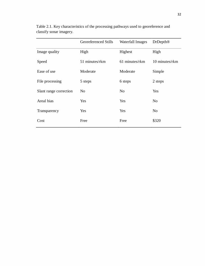
Three distinct processing methods were used to convert raw sonar images to sonar
image mosaics (SIMS) (Table 2.1). The georeferenced still (GS) approach used still,
waterfall images, named for the way in which the image cascades down a screen when
viewed in real time (Figure 2.3). These images can either be screen captures from the
head unit or in this case, still images extracted from video recordings created by the sonar
head unit. While some distortion was introduced to the images in the georeferencing
process, nearly the full detail of the original images was maintained. This process did not
correct for slant range distortion. The water column was present in the end product, and
the georeferenced images are not strictly accurate in terms of area. Similar approaches

21
have required approximately 51 minutes per rkm mapped for image preparation and
georeferencing (Kaeser & Litts 2010.)
In this approach, Humminbird® video files were converted to still images and
then georeferenced in ArcMap 9.3 (Figure 2.4). The .dat files were first converted to the
eXtended Triton Format (.xtf) (Triton Imaging, Inc. 2008). Once converted to .xtf, the
recordings were opened in SIView (Norwood 2010), and exported as a series of bitmaps
(.bmp), each corresponding to a 100-meter stream length. GPS waypoint and track data
were exported in SIView as a text (.txt) file, imported into ArcMap 9.3, and saved as an
ESRI shapefile. The shapefiles were then used to create an image-to-ground control point
network consisting of 300 to 360 points per image in the set using the ArcGIS toolset
developed by Kaeser & Litts (2008). The images were rectified to the ground control
points at a pixel resolution of 10 cm. The resulting SIMs were saved as .png images with
corresponding world files registered to UTM Zone 17 and projected on the North
American Datum of 1983 (NAD83).
I used the same methods in the second, waterfall (WF) approach, but classified
the substrate from waterfall images prior to georeferencing the images. The intent of this
method was to achieve the highest quality images for classification, in hopes of achieving
greater accuracy. Georeferencing introduces warping and a distortion to the waterfall
images, in light of this, the highest quality imagery is seen prior to such manipulations.
This is especially true when navigational constraints force deviation from straight lines
surveys, where waterfall images do not correspond to linear travel. This approach
required an additional processing step, and approximately 61 minutes per rkm mapped.
However, the maps created are already classified.

22
The waterfall processing approach utilized the same processing tools as the
georeferenced stills approach, but applied them to classified imagery. Sonar files were
processed with Son2XTF and SIView to create a series of .bmp files. The .bmp files were
then opened in ArcMap 9.3. A new shapefile was created and populated with polygons
corresponding to unique substrate patches from the sonar images; this shapefile was then
exported as a .bmp. Adobe Photoshop CS5 was used to remove a border region
introduced in the export from ArcMap and to resize the classified image to the same
proportions as the original sonar image. This image was again saved as a .bmp and
processed in the exact manner as the unprocessed images to create SIMs.
The final approach (DD), the side-scan extension for the DrDepth® software
package, is able to directly read the Humminbird® sonar recordings. The recordings are
georeferenced without an intermediary still image, and are slant range corrected. This
allows for accurate measurement of area and an end product without the artifact of the
water column. This approach is the fastest of the three, requiring no more than 10
minutes per rkm mapped for georeferencing, and no image preparation. However, the
additional manipulation of the image may reduce detail.
This path used DrDepth® to read the .dat files and rapidly generate SIMs. The
.dat files were loaded into DrDepth® and opened at resolution of 12.5 cm per pixel. The
images were exported as .bmp files with accompanying Google Earth .kml files. The .kml
files were used to generate world files and the .bmp's were opened in ArcMap and
projected onto NAD83, UTM Zone 17.
A classification scheme was determined from field observations and included four
distinct classes, covering the dominant substrate types observed in the Ogeechee River.

23
The classes were sandy (S), hard-packed clay (C), gravel (G) and exposed bedrock (B)
(Figure 2.5). Points designated sand were composed entirely of sand. Ground truth points
were assigned to one of the non-sand classes if any amount of the substrate type in
question was present. A minimum map unit (MMU) was defined in the field as one
square-meter, or the approximate extent visible using the underwater camera.
Of the four reaches surveyed, one was held back as a training section and
classified with the assistance of the reference data for that reach. The remaining the
stretches were visually, or “heads up,” classified without foreknowledge of the reference
data for those reaches. For consistency, all heads-up classification was conducted by the
same observer. In all approaches, substrate classification of the SIMs was conducted in
ArcMap 9.3. New shapefiles were created and populated with polygons corresponding to
unique areas of contiguous like substrate greater than the MMU. The polygons were then
assigned to one of the four substrate classes. The streambed was classified from bank to
bank, with areas of shadow or uncertainty classified as such (figure 2.6).
Error matrices and classification accuracy statistics were calculated using
reference data for all three processing approaches (Congalton and Green, 1999). In each
instance reference points occurring within 3 meters of a substrate class boundary or
within the water column of the un-slant range corrected SIMs were discarded, in an effort
to minimize classification errors due to positional error.
RESULTS
We mapped 2441 linear meters of the Ogeechee River. Due to the effects of slant
range distortion and variance across methods in classifying stream banks, area mapped

24
varied by method - for a total of 8.01 hectare using GS, 8.97 ha using WF, and 10.03 ha
using DD. Across all methods sand was the most common substrate identified,
composing 75% of classified substrate using GS, 66% using WF, and 71% using DD
(Tables 2.2, 2.3, & 2.4). The remaining classified areas were 14% exposed bedrock and
7% clay using GS; 17% bedrock, 6 % clay, and 3 % gravel using WF; and 18% bedrock,
8% clay, and 1% gravel using DD. Unsure areas totaled 4%, 7%, and 3% using GS, WF,
and DD, respectively.
Overall classification accuracy was 85% using WS, 83% using WF, and 82%
using DD. Producer’s accuracy, or errors of omission, ranged from 0% to 98% with WS,
16% to 95% with WF, and 39% to 94% with DD. User’s accuracy, or errors of
commission, ranged from undefined to 93% using WS, 59% to 94% using WF, and 28%
to 93% using DD. Undefined value were the result of no gravel being classified using
GS, which resulted in a zero in the denominator when calculating user's accuracy. Kappa
analysis of the error matrices resulted in a KHAT of 0.75 with WS, 0.73 with WF, and
0.70 with DD (Table 2.5), suggesting moderate to good agreement with the reference data
(Landis and Koch 1977). Pairwise comparison of the error matrices yielded no Z statistic
greater than 0.42 (Table 2.6), indicating that there was no significant difference between
the matrices.
DISCUSSION
While error matrices among the three side-scan sonar processing approaches
showed no statistical difference, there were some patterns worth noting. Across methods,
classification accuracy was highest in the most common classes -- sand and bedrock.

25
These two classes were also frequently over-predicted, with producer’s accuracy often
notably higher than user's. This may be an artifact of the reference data sampling, as
systematic sampling tends to over-represent common classes (Congalton and Greene
1999). Combined with the ubiquity of sand and bedrock in the survey sites, this may have
led to habituated over-classification during the inherently subjective heads-up
classification.
Classification of clay was also fairly successful; user’s accuracy was highest in
the clay class across all methods. Additionally, the clay substrate was found in one large
and continuous patch. As one of the key difficulties in classification is discriminating
boundaries in transition zones, this minimized a main source of error (Meyer and White
2007). Consolidated clay sediments only occurred at one of the survey locations, which
may have minimized opportunities for over-prediction, as there were effectively only two
clay/non-clay boundaries in the study area.
The most common source of error across all methods was difficulty in
distinguishing between classes during heads-up classification. The gravel class was most
problematic with no method resulting in a producer’s accuracy higher than 39% in this
class. Much of the difficulty in correctly classifying gravel lies in its similarity to other
classes on the SIMs. In all methods except DD, gravel was more frequently classified as
sand than correctly identified. Gravel was the rarest class, comprising no more than
10.5% of reference data; as such, there were little in the realm of training opportunities.
Additionally, many of the samples identified in the field as gravel were mixtures of sand
and gravel. Likewise, this patchiness may have compounded positional error, as some

26
patches were smaller than the stated accuracy of the Humminbird® GPS – 3m
(Humminbird 2007).
No gravel was successfully identified using GS. This was not due to an inability
of the method to identify gravel, but rather to a drawback to the GS method. The sole
patch of gravel in the survey areas was located in an area that required great deviation
from straight line travel due to obstacles in the river channel. This resulted in waterfall
images that could be interpreted and classified with difficulty. Deviation from straight
line surveying likely suppressed classification accuracy across all methods, but the effect
was most severe in the GS approach. When a control grid was created from the track
data, the resultant rectified imagery was greatly distorted and no classification could be
made using the imagery. While this effect can be minimized by georeferencing more and
smaller waterfall images, it also illustrates the importance of maintaining straight line
surveying paths. DD was the least affected by deviation from straight line surveying
paths.
Discrimination between gravel and sand may be an inherent challenge to
recreational-grade side scan sonar due to limited along track, or transverse resolution
(Kaeser and Litts 2010) - which is the smallest recognizable detail of an image produced
along a line parallel to the towpath (Fish and Carr 1990). Humminbird® side-scan sonar
equipment has a stated transverse resolution of 63.5 mm (Humminbird 2007). This
limitation results in SIMs that display similar appearances for all particles under 63.5 mm
in size. In contrast, research oriented equipment operates at along track resolutions as low
as 18 mm (EdgeTech 2011). Contextual cues and larger patterns in substrates can offset
this limitation, especially in heads-up classifications (Kaeser and Litts 2010).

27
Overall accuracy was similar across all methods and compares well to previous
studies. Overall accuracy in the only published study using Humminbird® side-scan
equipment to classify stream substrate was 76%, 86% when the rocky substrate classes
were simplified from three classes to two (Kaeser & Litts 2010). The overall accuracy of
all methods here falls into that range. Similarly, lowest classification accuracy was seen
in gravel substrates.
Limited substrate diversity in the Ogeechee River may have also contributed to
poor differentiation among substrate classes. Low gradient southeastern rivers are
frequently dominated by sandy substrate (Wallace & Benke 1984, Benke et al. 1985), and
in this case, only a few small patches of rocky substrates could be located. The
dominance of sand substrates likely hindered accurate classification of rocky substrates
due to a lack of training opportunities. Regardless of which processing method is used,
visual classification of stream substrate is a subjective process with a steep learning
curve. Additional training opportunities with a variety of course substrates would have no
doubt lead to greater classification accuracy. Repeating this study on a higher gradient
stream likely would result in greater classification accuracy of rocky substrate classes.
Given the lack of statistical difference between approaches, and the speed and
ease of use, I suggest that the DrDepth® approach is the most preferable method for
georeferencing sonar imagery created by Humminbird® equipment. While overall
accuracy was lowest with DD, this difference was not significant. There may also be
training issues at play with DrDepth®. The SIView based approaches display the sonar
images in a familiar way to the classifier; appearing very much as they do on the sonar
head unit. DrDepth® in addition to generating images that appear comparatively

28
unfamiliar had only been available for a few months at the time of classification. It is
possible that with greater familiarity to these images, classification accuracy would
improve.
Correction of slant range error is another reason to favor DD. Slant range
corrected images offer a “bank to bank” picture of the river bottom and allow accurate
measurements of area. Elimination of the water column in the image also provides a more
intuitive picture of the river bottom. This feature alone may result in a superior end
product, especially when creating maps for a non-technical audience. Slant range
correction in DrDepth® does require resampling and remapping of the sonar imagery,
and a subjective loss in image quality. This may be largely avoided by retaining
uncorrected imagery for use as a reference when classifying corrected SIMs.
Conclusion
This study presents an evaluation of currently available processing tools for
recreational-grade side-scan sonar imagery, which will assist in the application of this
emerging technology. DrDepth® can be used to rapidly generate georectified images of
benthic habitat with accuracy similar to more labor-intensive approaches. These tools can
be used to efficiently examine aquatic habitat at a high level of detail without the
limitations posed by transect based sampling in turbid or non-wadeable streams and
lakes.

29
Literature Cited
Balian, E. V., H. Segers, C. Leveque, and K. Martens. 2008. The Freshwater Animal
Diversity Assessment: an overview of the results (vol 595, pg 627, 2008).
Hydrobiologia. 600: 313-313.
Benke, A. C., R. L. Henry, D. M. Gillespie, and R. J. Hunter. 1985. Importance of snag
habitat for animal production in southeastern streams. Fisheries 10: 8-13.
Benke, A. C. 1990. A perspective on America’s vanishing streams. Journal of the North
American Benthological Society 9: 77-88.
Blondel, P. 2009. Handbook of Sidescan Sonar. Springer-Praxis. New York, New York.
Cobra, D. T., A. V. Oppenheim, and J. S. Jaffe. 1992. Geometric distortions in side-scan
sonar images - a procedure for their estimation and correction. Ieee Journal of
Oceanic Engineering. 17: 252-268.
Congalton, R.G. and K. Green. 1999. Assessing the Accuracy of Remotely Sensed Data:
Principles and Practices. Lewis Publishers. Boca Raton, Florida.
Edgetech. 2011. 2400 Series Deep Towed Side-Scan Sonar and Sub-Bottom Profiling
System. Retrieved form www.edgetech.com/edgetech/gallery on March 2, 2011.
Fausch, K. D., C. E. Torgersen, C. V. Baxter, and H. W. Li. 2002. Landscapes to
riverscapes: Bridging the gap between research and conservation of stream
fishes. Bioscience. 52: 483-498.
Fish, J. P. and H.A. Carr. 1990. Sound underwater images. Lower Cape Publishing,
Orleans, Massachusetts.
Fleming, J. E., T. D. Bryce, and J. P. Kirk. 2003. Age, growth, and status of shortnose
sturgeon in the Lower Ogeechee River, Georgia. Proceedings of the Annual
Conference Southeastern Association of Fish and Wildlife Agencies. 57: 80-91.
Gleick, P. H. 1996. Basic water requirements for human activities: Meeting basic needs.
Water International. 21: 83-92.
Humminbird. 2007. 997SI Installation and Operations Manual. Eufala, Alabama.
Jelks, H. L., S. J. Walsh, N. M. Burkhead, S. Contreras-Balderas, E. Diaz-Pardo, D. A.
Hendrickson, J. Lyons, N. E. Mandrak, F. McCormick, J. S. Nelson, S. P.
Platania, B. A. Porter, C. B. Renaud, J. J. Schmitter-Soto, E. B. Taylor, and M. L.
Warren. 2008. Conservation Status of Imperiled North American Freshwater and
Diadromous Fishes. Fisheries. 33: 372-407.

30
Kendall, M. S., O. P. Jensen, C. Alexander, D. Field, G. McFall, R. Bohne, and M. E.
Monaco. 2005. Benthic mapping using sonar, video transects, and an innovative
approach to accuracy assessment: A characterization of bottom features in the
Georgia Bight. Journal of Coastal Research. 21: 1154-1165.
Krakow, G. Known occurrences of special concern plants, animals, and natural
communities in Ogeechee River, upper watershed (HUC8: 03060201). Georgia
Department of Natural Resources. Retrieved from
www.georgiawildlife.com/node/1372 on March 2, 2011.
Landis, J. R. and G. G. Koch. 1977. Application of hierarchical kappa-type statistics in
assessment of majority agreement among multiple observers. Biometrics. 33:
363-374.
Levin, P. S. and G. W. Stunz. 2005. Habitat triage for exploited fishes: Can we identify
essential "Essential Fish Habitat?". Estuarine Coastal and Shelf Science. 64: 70-
78.
Lucieer, V. L. 2008. Object-oriented classification of sidescan sonar data for mapping
benthic marine habitats. International Journal of Remote Sensing. 29: 905-921.
Mertes, L. A. K. 2002. Remote sensing of riverine landscapes. Freshwater Biology. 47:
799-816.
Meyer, J. L., A. C. Benke, R. T. Edwards, and J. B. Wallace. 1997. Organic matter
dynamics in the Ogeechee River, a blackwater river in Georgia, USA. Journal of
the North American Benthological Society. 16: 82-87.
Meyer, J. D. and S. M. White. 2007. Lava morphology mapping by expert system
classification of high-resolution side-scan sonar imagery from the East Pacific
Rise, 9 degrees-10 degrees N. Marine Geophysical Researches. 28: 81-93.
Norton, M. 2010. SIView 1.0+. www.mnorwood.com/SIView.
Perlin, P. 2010. DrDepth Sea Floor Mapping Software. Version 2.0
Göteborg, Sweden. www.drdepth.se.
Strayer, D. L., H. M. Malcom, R. E. Bell, S. M. Carbotte, and F. O. Nitsche. 2006. Using
geophysical information to define benthic habitats in a large river. Freshwater
Biology. 51: 25-38.
Triton Imaging, Inc. 2008. eXtended Triton Format(XTF) Revision
26.capitola, California. http://www.tritonimaginginc.com.
USGS (U.S. Geological Survey) 2011. USGS 02203536 Ogeechee river at US 17, near
Richmond Hill, GA. Retrieved from

31
http://waterdata.usgs.gov/ga/nwis/uv/?site_no=02203536&PARAmeter_cd=0006
5,00060,00062 on March 2, 2011.
Wallace, J. B. and A. C. Benke. 1984. Quantification of wood habitat in sub-tropical
coastal-plain streams. Canadian Journal of Fisheries and Aquatic Sciences. 41:
1643-1652.
Wiens, J. A. 2002. Riverine landscapes: taking landscape ecology into the water.
Freshwater Biology. 47: 501-515.
Witte, T. H. and A. M. Wilson. 2005. Accuracy of WAAS-enabled GPS for the
determination of position and speed over ground. Journal of Biomechanics. 38:
1717-1722.
32
Table 2.1. Key characteristics of the processing pathways used to georeference and
classify sonar imagery.
Georeferenced Stills Waterfall Images DrDepth®
Image quality High Highest High
Speed 51 minutes/rkm 61 minutes/rkm 10 minutes/rkm
Ease of use Moderate Moderate Simple
File processing 5 steps 6 steps 2 steps
Slant range correction No No Yes
Areal bias Yes Yes No
Transparency Yes Yes No
Cost Free Free $320

33
Table 2.2. Error matrix for georeferenced stills approach.
Classified data Reference site data (field data) Row total
User’s accuracy B C G S
B 164 0 9 35 208 78.85%
C 0 53 4 0 57 92.98%
G 0 0 0 0 0 n/a
S 3 15 20 273 311 87.78%
Column total 167 68 33 308 576
Producer’s accuracy 98.20% 77.94% 0.0% 88.64% Overall
accuracy
85.07%

34
Table 2.3. Error matrix for waterfall image approach.
Classified data Reference site data (field data) Row total
User’s accuracy B C G S
B 161 0 25 29 215 74.88%
C 0 51 3 0 54 94.44%
G 7 0 10 0 17 58.82%
S 2 11 26 282 321 87.85%
Column total 170 62 64 311 607
Producer’s
accuracy
94.71
%
82.26
%
15.63
%
90.68
%
Overall accuracy
83.03%

35
Table 2.4. Error matrix for DrDepth® approach.
Classified data Reference site data (field data) Row total
User’s accuracy B C G S
B 192 0 5 57 254 75.59%
C 0 53 4 0 57 92.98%
G 11 0 15 27 53 28.30%
S 2 11 14 321 348 92.24%
Column total 205 64 38 405 712
Producer’s accuracy 93.66% 82.81% 39.47% 79.26% Overall accuracy
81.60%

36
Table 2.5. Error matrices analysis statistics.
Matrix KHAT Variance Z
Georeferenced Still 0.749 0.00935 7.74
Waterfall 0.725 0.00754 8.35
DrDepth® 0.697 0.00589 9.08

37
Table 2.6. Pairwise comparison analysis of variance between error matrices.
Pairwise Comparison Z Statistic
Georeferenced Still vs. Waterfall 0.188
Georeferenced Still vs. DrDepth® 0.418
Waterfall vs. DrDepth® 0.241

38
Figure 2.1. An representative side-scan sonar image from the Ogeechee River, Georgia.
Legend as follows; A: stream bank, B: first surface return, C: trigger pulse, D: first
bottom return, E: shadow, F: woody debris, G: water column (Adapted from Fish and
Carr, 1990).

39
Figure 2.2. Study locations on the Ogeechee River, Georgia.

40
Figure 2.3. Waterfall (left) and georeferenced (right) side scan sonar imagery.

41
Figure 2.4. File processing pathways for Georeferenced Stills, Waterfall Image, and
DrDepth® approaches.

42
Figure 2.5. Interpretation key to four classes of stream substrate on the Ogeechee River,
Georgia.

43
Figure 2.6. Sample sonar image map created from Dr. Depth imagery recorded in the
Ogeechee River, Georgia.

44
CHAPTER THREE
IDENTIFICATION OF POTENTIAL ATLANTIC STURGEON SPAWNING
GROUNDS IN THE OGEECHEE RIVER, GEORGIA USING LOW-COST SIDE-
SCAN SONAR1
1Hook, J.D., D.L. Peterson, and N.P. Nibbelink. To be submitted.

45
Abstract
As a group, sturgeon are among the world’s most imperiled fish. In the Ogeechee River,
Georgia, recovery of a small but unquantified population of Atlantic sturgeon (Acipenser
oxyrinchus oxyrinchus) is impeded by loss of nursery habitats and thermal refugia, as
well as bycatch from a shad fishery. Knowledge of spawning habits is vital for the
successful management and restoration of imperiled anadromous fish. However, most
knowledge of Atlantic sturgeon spawning locations comes from northern rivers. There
has been little work on locating spawning grounds in southern systems. Our primary
objective was to define potential spawning locations for Atlantic sturgeon in the
Ogeechee River of Georgia. A second objective was to demonstrate the application of
low cost sonar survey techniques to a pressing conservation and management issue.
These objectives were addressed by mapping stream reaches containing suitable
spawning habitats using imagery from recreational-grade Humminbird® side-scan and
multi-beam sonar equipment. We identified all hard substrates greater than 1.5 m depth
as potentially suitable for sturgeon spawning. Eight stream reaches totaling 50,892 square
meters were identified as potentially suitable for spawning use by Atlantic sturgeon,
representing about 0.2% of the total estimated area of river-bottom. Especially where
depth or turbidity precludes traditional habitat sampling, this approach offers an efficient
method for locating habitat types for further targeted investigation. Recreational-grade
sonar surveying is particularly useful in low-gradient Southeastern streams like the
Ogeechee River, where habitat types of interest may be uncommon and scattered over
hundreds of river kilometers.

46
INTRODUCTION
As a group, sturgeon are among the world’s most imperiled fish. Worldwide, 23
of 25 species are categorized as threatened or endangered by the International Union for
Conservation of Nature and Natural Resources (IUCN) Red List (IUCN 2010). Presently,
Atlantic sturgeon (Acipenser oxyrinchus oxyrinchus) are classified as Near Threatened
(Pierre and Paruka 2006), and the National Marine Fisheries Service has proposed listing
four of the five Distinct Population Segments (DPS) recognized in the United States as
endangered under the Endangered Species Act (NMFS 2010 NMFS 2010a). Threats to
Atlantic sturgeon include loss of habitat through dams and dredging, pollution, and
mortality associated with bycatch (Smith and Clugston 1997). In the Ogeechee River,
Georgia, recovery of a small but unquantified population of Atlantic sturgeon is impeded
by loss of nursery habitats and thermal refugia, as well as bycatch from the shad fishery
(NMFS 1998).
Atlantic sturgeon are the largest anadromous fish of the North American Atlantic
coast and range historically from Labrador, Canada to the Gulf of Mexico (NMFS 1998).
Their current range is diminished to populations using 20 Atlantic coastal rivers (ASSRT
2007). Population declines began soon after the emergence of a large commercial fishery
in the late nineteenth century (Secor and Waldman 1999). Harvest peaked at 3350 metric
tons in 1890, and collapsed within 10 years, due to persistent overharvest (Smith and
Clugston 1997, Secor and Waldman 1999). Landings continued at one percent of peak
levels for most of the 1900's until the Atlantic States Marine Fisheries Commission
imposed an emergency moratorium in December of 1995 (Bain et al. 2000, ASMFC

47
1998). The moratorium was made permanent in 1998, however, commercial harvest
continues in Canadian waters.
Knowledge of spawning habits is vital for the successful management and
restoration of imperiled anadromous fish. However, most knowledge of Atlantic sturgeon
spawning locations comes from northern rivers. There has been little work on locating
spawning grounds in southern systems. Atlantic sturgeon broadcast adhesive eggs into
the demersal zone upstream of the saltwater interface (Gilbert 1989, Collins et al. 2000,
Hatin et al. 2002). Spawning grounds occur at least 20 to 100 rkm upstream, with some
sites documented at much as 221 rkm upstream (Van Eenennaam et al. 1996, Armstrong
and Hightower 2002). Atlantic sturgeon spawning sites are characterized by the presence
of hard bottom substrate such as rock, rubble, or hard clay (Table 3.1). In low gradient
southern rivers, these conditions are often expressed as rock or limestone outcroppings
(Gilbert 1989). Depth of documented spawning sites ranges from a minimum of 1.5 m to
a maximum of 60 m (Van Den Avyle 1984, Collins et al. 2000, Caron et al. 2002, Hatin
et al. 2002).
There are several reasons why hard bottom substrates are required for spawning.
First, Atlantic sturgeon eggs are adhesive, and if deposited into sandy or other soft
bottoms they may become encapsulated, suffocating the developing egg (Van Den Avyle
1984, Fox et al. 2000). Second, developing sturgeon free embryos inhabit the interstitial
spaces between coarse, hard substrates (Kempinger 1988, LaHaye et al. 1992). Interstitial
spaces provide several key benefits to pre-larval sturgeon including protection from
predation and allow poor swimming free embryos to resist drift. Given that age 1 and
younger fish of most sturgeon species are intolerant of even very low salt concentrations

48
(Jenkins et al. 1993, Kynard and Horgan 2002), drifting into brackish water would be
lethal for developing larvae (Gessner et al. 2009). As such, interstitial spaces amongst
hard substrates are necessary to the survival of Atlantic sturgeon during the early critical
life stage.
There are no recent studies quantifying the abundance of Atlantic sturgeon in the
Ogeechee River, however Atlantic sturgeon are believed to spawn in the river based on
the presence of Age 1 juveniles. Farrae et al. (2009) estimated the abundance of age 1
Atlantic sturgeon in the Ogeechee River to be 450 in 2007, and numerous other
researchers have captured age 1 Atlantic sturgeon in the system. (Table 3.2). Age 1
sturgeon have not yet developed salinity tolerance and remain in their natal rivers, as such
the presence of age 1 Atlantic sturgeon in the Ogeechee River indicates that they were
spawned there. This assumes the presence of age 0 sturgeon as well, however it is
difficult to assess the presence of age 0 Atlantic sturgeon as they are not vulnerable to
capture in entanglement gear (Schueller and Peterson 2010).
While the frequent presence of age 1 sturgeon indicate that Atlantic sturgeon are
spawning in the Ogeechee River, little is known about their spawning grounds. Our
primary objective was to define potential spawning locations for Atlantic sturgeon in the
Ogeechee River of Georgia. A second objective was to demonstrate the application of
low cost sonar survey techniques to a pressing conservation and management issue.
These objectives were addressed by mapping stream reaches containing suitable
spawning habitats using imagery from recreational-grade Humminbird® side-scan and
multi-beam sonar equipment.

49
Study area - the Ogeechee River
At 394 kilometers, the Ogeechee River is the longest unimpounded river in
Georgia, and one of 42 free-flowing rivers greater than 200 kilometers in the lower 48
states (Benke 1990). A sixth order river, the Ogeechee River drains a watershed of
14,300 square kilometers. The Ogeechee River’s headwaters are in the Georgia Piedmont
and the majority of its length and 95 percent of its drainage is located in the Coastal plain
(Meyer et al. 1997). Below a small falls near Shoals, Georgia the river becomes a slow
blackwater river with an average daily discharge of 115 cubic meters per second (Meyer
et al. 1997). Spring flooding swells discharge to an average daily discharge of 146.4
during the month of March. The Ogeechee River has one major tributary, the Canoochee
River -- a 160 kilometer long stream which joins the Ogeechee River at river kilometer
55 (Fleming et al. 2003).
METHODS
Side scan and multi-beam sonar surveys were performed on the Ogeechee River
from river kilometer (rkm) 32 near Fort McAllister to approximately rkm 320 near
Louisville, Georgia from January 2009 to June 2009. Surveys were performed at high
flows to capture bank full width while minimizing navigational difficulties. The surveys
were conducted using Humminbird® 997SI side scan and 967C multi-beam sonar
systems. The 997SI sonar transducer was mounted to a boom off the bow of the 13.5 foot
Riverhawk ghanoe to minimize wake-induced turbulence. The 967C sonar transducer
was mounted to the transom, as it is relatively unaffected by wake. In both cases, the GPS

50
antenna was mounted to the top of the boom, directly above the transducer, to maximize
locational accuracy. Operating frequency was set to 455 kHz. Range was set to 150% of
estimated stream width, as little as 20 meters at upstream sites and as much as the
maximum range of the units, 100 meters, at lower locations. Side-scan sonar imagery was
captured while navigating downstream at midchannel at 5.5 kph (3 knots). Bathymetric
data was collected while navigating either upstream or downstream at speeds from 5.5 to
8.0 kph (3 to 5 knots). At least three and as many as seven passes were made at each site
using the 967 system at positions spread evenly across the channel to maximize coverage.
Sonar recordings were stored in the Humminbird® proprietary .dat/.son format. The
.dat/.son format is intended for playback on the head unit on which it was recorded, or on
that of a similar model. This format is similar to a video recording of the sonar imagery.
Side-scan recordings were converted to the eXtended Triton Format (.xtf) (Triton
Imaging, Inc. 2008) using Son2XTF 1.001 (Humminbird 2008). Once converted to .xtf
the side scan recordings were georeferenced using DrDepth® 3.9.23 (Perlin 2010). The
recordings were georeferenced without slant- range correction at a 0.0625 meter per pixel
resolution, and exported as .png image files with accompanying Keyhole Markup
Language (.kml) files. ESRI World files were manually derived from the .kml files and
the georeferenced images were projected in NAD83 in ESRI ArcMap 9.
In order to determine potentially suitable locations for Atlantic sturgeon
spawning, I examined substrate type and depth. Stream substrate was manually
interpreted and classified (“heads up” classification). Aerial photography was used to aid
classification, primarily when identifying landowner placed rip rap and bank
improvements. Stream substrate was classified into two categories, either potentially

51
suitable for spawning use by Atlantic sturgeon, or unsuitable. While specific substrate
associations with Atlantic sturgeon spawning grounds in literature are varied, nearly all
described spawning locations contain some form of hard bottom substrate (Musick 2005).
Thus, the potentially suitable class consisted of all hard substrates – exposed bedrock,
cobble, gravel, boulders, and hard consolidated sediments. All other substrate types were
classified as unsuitable. Areas of potentially suitable substrate were digitized as
polygons. No efforts were made to further discriminate substrate type in areas deemed
unsuitable.
Multi-beam data collected with the 967C was used to construct a bathymetric
profile of stream reaches containing potentially suitable substrates. The .dat output of the
Humminbird® sonar was converted to .xtf and then imported to MBSystem (Caress &
Chayes 2009). The raw sonar data was exported as comma separated text files consisting
of longitude, latitude, and depth values. Obvious outliers and spurious points were
filtered by eliminating any points with depths less than zero or greater than 30 meters.
The remaining points, at least 30 per river meter, were imported to ArcMap 9.2 and
projected into NAD83. Side scan images were used to digitize the stream banks. A depth
profile of the potentially suitable reaches during springtime flows was then created using
Inverse Distance Weighting to interpolate between the digitized banks and the multi-
beam swaths. The minimum depth associated with a documented Atlantic sturgeon
spawning location is 1.5 m (Collins et al. 2000); therefore, this depth was deemed the
minimum potentially suitable depth in this study.

52
RESULTS
I surveyed the Ogeechee River from rkm 30, near Fort McAllister, to rkm 320, near
Louisville, GA, for a total of 298 rkm, from January to May 2009. Of these, approximately 272
rkm were survey above the furthest upstream occurrence of the salt wedge, at approximate rkm
56 (GADNR 2001). Navigational difficulties prevented surveying the river above rkm 320. As
such, the river was not surveyed to the fall line, at approximate rkm 350.
Potentially suitable substrates found included exposed limestone bedrock, small
limestone boulders, coarse gravel, hard-consolidated clay, and landowner placed rip rap.
The remaining substrates identified consisted of sand, soft clay, and silt sediments.
Surveyed depths ranged from 0.2 meters to 12.8 meters.
Eight stream reaches totaling 50,892 square meters were identified as potentially
suitable for spawning use by Atlantic sturgeon (Table 3.3, Figure 3.1). This represents
0.2% of the roughly 23,900,000 m2 surveyed. Of the 50,892 m
2 identified, 34,949 m
2 or
68% were naturally occurring hard substrates. The remaining15,943 m2 consisted of
introduced gravel and rip rap.
Depths at these locations during the survey periods ranged from 1.1 meters at the
most downstream reach at river kilometer (rkm) 84.3 to a maximum depth of 5.6 meters
at one of the most upstream reaches at rkm 219.6. Survey dates for these reaches were
from February 23 to March 12, 2009. The Ogeechee River rose by more than three meters
over the following two weeks, as such all reaches identified as containing suitable
substrates would have met minimum depth requirements at some point during the
February through April time-frame for Atlantic sturgeon spawning movements in
southern rivers (Musick 2005, Greene et al. 2009).
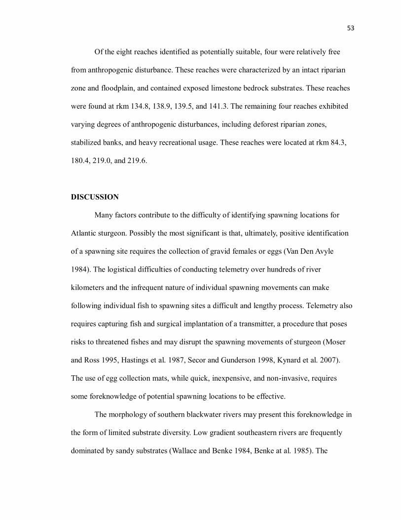
53
Of the eight reaches identified as potentially suitable, four were relatively free
from anthropogenic disturbance. These reaches were characterized by an intact riparian
zone and floodplain, and contained exposed limestone bedrock substrates. These reaches
were found at rkm 134.8, 138.9, 139.5, and 141.3. The remaining four reaches exhibited
varying degrees of anthropogenic disturbances, including deforest riparian zones,
stabilized banks, and heavy recreational usage. These reaches were located at rkm 84.3,
180.4, 219.0, and 219.6.
DISCUSSION
Many factors contribute to the difficulty of identifying spawning locations for
Atlantic sturgeon. Possibly the most significant is that, ultimately, positive identification
of a spawning site requires the collection of gravid females or eggs (Van Den Avyle
1984). The logistical difficulties of conducting telemetry over hundreds of river
kilometers and the infrequent nature of individual spawning movements can make
following individual fish to spawning sites a difficult and lengthy process. Telemetry also
requires capturing fish and surgical implantation of a transmitter, a procedure that poses
risks to threatened fishes and may disrupt the spawning movements of sturgeon (Moser
and Ross 1995, Hastings et al. 1987, Secor and Gunderson 1998, Kynard et al. 2007).
The use of egg collection mats, while quick, inexpensive, and non-invasive, requires
some foreknowledge of potential spawning locations to be effective.
The morphology of southern blackwater rivers may present this foreknowledge in
the form of limited substrate diversity. Low gradient southeastern rivers are frequently
dominated by sandy substrates (Wallace and Benke 1984, Benke at al. 1985). The

54
Ogeechee River is typical of these systems with an average elevation change in the study
area of 0.00028 m/m. I identified only five natural patches of hard bottom. Though there
is little documentation of the spawning substrate preferences of southern populations of
Atlantic sturgeon, given the importance of interstitial spaces within coarse substrates, it is
reasonable to assume they, like northern populations, exclusively utilize hard bottom
areas. Therefore, it is likely that Atlantic sturgeon spawning locations in the Ogeechee
River are limited to these hard bottom locations. Targeted sampling for eggs or pre-larval
sturgeon may be used to confirm the use of these locations as spawning grounds by
Atlantic sturgeon.
Although no verification data were collected in this survey, previous work using
similar techniques and equipment demonstrated the effectiveness of these methods.
Kaeser and Litts (2010) used Humminbird® side-scan sonar and heads up classification
to delineate substrate in the Ichawaynochaway Creek, Georgia to four classes with an
overall classification accuracy of 77%. A large portion of the classification errors in their
study were between rocky classes, when coarse substrates were folded into only two
classes, overall accuracy improved to 86%. Similarly Hook et al. (in prep) found an
overall accuracy of 81.6% classifying substrates in the Ogeechee River using
Humminbird® sonar, DrDepth® software, and heads up classification.
A large portion of error in both of these studies was found in the borders between
different substrate patches (Kaeser and Litts 2010, Hook et al. in prep). Border error is a
result of positional error and the difficulty in identifying precise transition points between
substrate types. These results suggest that patch interiors are typically assigned to the
correct classes, but the borders, and therefore areal measurements, are subject to error.

55
Compounding errors in areal measurement is additional error introduced through slant
range distortion, the difference between the distance from the sonar sensor to a given
point perpendicular to the trackline and the true across track distance to that point (Fish
and Carr 1990). This distortion results in a given point appearing further away from the
sensor across track than it is in reality, with the greatest displacement directly underneath
the sensor. The distortion can be roughly estimated at any point across track by using the
Pythagorean Theorem. Assuming constant depth, the true across track distance is
equivalent to the square root of the difference of the squared apparent distance along
track and the squared depth under the sensor (Blondel 2009). At the shallow depths
observed in this study, the effect is small. The area of a substrate patch that extended from
bank to bank would be exaggerated by at most 2%.
Correcting for slant range error is preferred and would reduce areal measurement
error, but this was not possible with Humminbird® sonar recordings made prior to the
4.57 firmware version. However, correcting for slant range error does compromise image
quality, as it requires resampling and remapping the sonar imagery. In a prior study using
these techniques, image degradation was noticed, but it did not result in a significant
difference in classification accuracy (Hook et al. in prep). Given access to the most recent
versions of Humminbird® firmware and DrDepth®, I recommend classifying slant range
corrected imagery, while using uncorrected georeferenced images as a visual reference.
While it is likely that some extant hard bottom areas were not identified, coarse
substrates are rare on the Ogeechee River. The extremely low gradient and wide
floodplain of the Ogeechee limits occasions were high flows would scour the riverbed
(Benke et al 1985), and sandy substrates dominate the river. However, where the riparian

56
zone is developed, coarse substrates are often introduced in the form of bank
modifications. The Ogeechee River has a wide and flat riparian zone that typically floods
in March and April (Benke et al. 1985), and a substantial amount of introduced rip rap is
needed to create a permanent artificial bank. Bank stabilization measures are most often
used in outside river bends and other incised areas. Due to distance from and angle to the
sonar transducer, these features can be among the hardest to discriminate in side-scan
imagery. While a large flood plain and limited road access limits development of the
banks of the Ogeechee River, there are likely more patches of rip rap that I failed to
detect. While there is no evidence that Atlantic sturgeon spawn over rip rap, these areas
do meet the minimum standards I applied. Spawning over introduced substrates is not
unheard of among acipensers, as lake sturgeon (Acipenser fulvescens) have been
documented spawning over a variety of introduced substrates including rip rap placed by
private landowners for bank stabilization (Priegel and Wirth 1974, Bruch and Binkowski
2002, Caswell et al. 2004, Johnson et al. 2006).
Overall, this method presents a highly effective “first-cut” approach for locating
substrates of interest. At 12 minutes per rkm on the water and 10 minutes per rkm for
projection and interpretation (Hook et al. in prep), hard bottom areas can be identified far
more rapidly than is possible with transect based, physical sampling. This approach is
ideal for low gradient coastal plain rivers with little substrate diversity, where substrates
of interest may occur in small patches that may be missed entirely when using transect
based physical sampling.
Recreational-grade sonar surveying is an ideal technique in the Ogeechee River,
as it can be used to identify preferred spawning substrates for three listed species in the

57
watershed. In addition to Atlantic sturgeon, the Ogeechee River holds a small population
of federally endangered shortnose sturgeon (Acipenser brevirostrum), estimated at 203
individuals in 2009 (Farrae 2010). Shortnose sturgeon utilize coarse substrates as
spawning grounds similar to those favored by Atlantic sturgeon (Buckley and Kynard
1985, Kieffer and Kynard 1996). While the Ogeechee River shortnose sturgeon
population is considered a sink for the much larger Altamaha River population (Farrae
2010), preservation of potential spawning grounds may be critical to establishment of a
reproductive population in the Ogeechee.
The Ogeechee River is also home to a stocked population of robust redhorse
(Moxostoma robustum ), a species thought extinct until 1991 and classified as endangered
by the Georgia Department of Natural Resources (Freeman 1999). In an effort to
reestablish populations of this rare fish, 43, 048 robust redhorse have been stocked in the
Ogeechee River since 1997 (Slaughter 2011). Spawning robust redhorse utilize substrates
dominated by medium to coarse gravel located at depths from .29 to 1.1 meters (Freeman
and Freeman 2001). While this study struggled to identify gravel substrates, other
researchers have successfully located coarse gravel using these techniques (Kaeser and
Litts 2010). However, gravel is uncommon is the Ogeechee River, the only gravel
substrates I identified were introduced by the Southeast Aquatic Resources Partnership
and Georgia Division of Wildlife Resources in an effort to create spawning habitat for the
robust redhorse (SARP 2011).
Recreational-grade sonar surveying is not limited in application to low-
gradient southern rivers, and is well suited to rivers that share a suite of characteristics.
Critical characteristics of rivers for successful application of recreational-grade sonar

58
surveying are depth, current velocity, channel width, and canopy cover. The maximum
depth supported by Hummibird® side-scan sonar equipment is 45.7 meters (Humminbird
2005), while the minimum depth is that which is required for navigation. However, where
depth is great enough to allow the use of a research-grade sonar system and towfish,
recreational-grade equipment may not be the preferred choice. Ideal current velocity is
under four kph. Wake induced turbulence begins to degrade recreational-grade side-scan
sonar at speeds above five kph, higher speed surveying may be attempted if effective
efforts are made to isolate the transducer from the effects of turbulence. Humminbird®
side-scan sonar supports swath widths of up to 146 meters (Humminbird 2005), and
wider channel and lakes may be surveyed by creating seamed mosaics. However, signal
attenuation can degrade the image quality of large swaths – highest image quality with
this equipment is seen in channels less than 75 meters in width. A final consideration is
canopy cover; the canopy must be open enough to permit GPS reception.
Conclusion
Atlantic sturgeon successfully spawn in the Ogeechee River, as demonstrated by
the frequent presence of juvenile sturgeon. There remains a need to identify the exact
location of spawning grounds. Given the paucity of hard bottom areas in the Ogeechee
River, I feel the areas identified here have a very high potential for use by Atlantic
sturgeon. To confirm the use of these reaches as spawning grounds I recommend direct
sampling, using egg collection mats, at the patches identified here.

59
This study demonstrates the use of low cost recreational-grade sonar to identify
and map areas of interest in navigable waters. Especially where depth or turbidity
precludes traditional habitat sampling, this approach offers an efficient method for
locating habitat types for further targeted investigation. Recreational-grade sonar
surveying is particularly useful in low-gradient Southeastern streams like the Ogeechee
River, where habitat types of interest may be uncommon and scattered over hundreds of
river kilometers.

60
Literature Cited
Armstrong, J. L. and J. E. Hightower. 2002. Potential for restoration of the Roanoke
River population of Atlantic sturgeon. Journal of Applied Ichthyology. 18: 475-
480.
ASMFC (Atlantic States Marine Fisheries Commission). 1998. Review of the Atlantic
States Marine Fisheries Commission Fishery Management Plan for Atlantic
sturgeon (Acipenser oxyrhynchus). ASMFC, Washington, D.C.
ASSRT (Atlantic Sturgeon Status Review Team). 2007. Status review of Atlantic
sturgeon (Acipenser oxyrinchus oxyrinchus). Report to the National Marine
Fisheries Service, Northeast Regional Office, Gloucester, MA.
Bain, M., N. Haley, D. Peterson, J. R. Waldman, and K. Arend. 2000. Harvest and
habitats of Atlantic sturgeon Acipenser oxyrinchus Mitchill, 1815 in the Hudson
River estuary: Lessons for sturgeon conservation. Boletin Instituto Espanol de
Oceanografia. 16: 43-53.
Beechie, T. J., and Sibley, T. H. (1997). Relationships between channel characteristics,
woody debris and fish habitat in north-eastern Washington streams. Transactions
of the American Fisheries Society. 126: 217–29.
Benke, A. C., R. L. Henry, D. M. Gillespie, and R. J. Hunter. 1985. Importance of snag
habitat for animal production in southeastern streams. Fisheries. 10: 8-13.
Benke, A. C. 1990. A perspective on America’s vanishing streams. Journal of the North
American Benthological Society. 9: 77-88.
Blondel, P. 2009. Handbook of Sidescan Sonar. Springer-Praxis. New York, New York.
Caress, D. W. and D. N. Chayes. 2009. Mapping the Seafloor: Software for
the processing and display of swath sonar data. Columbia University.
Version 5.1.2.
Caron, F., Hatin, D. and Fortin, R. (2002), Biological characteristics of adult Atlantic
sturgeon (Acipenser oxyrinchus) in the St Lawrence River estuary and the
effectiveness of management rules. Journal of Applied Ichthyology. 18: 580–585.
Caswell, N. M., D. L. Peterson, B. A. Manny, and G. W. Kennedy. 2004. Spawning by
lake sturgeon (Acipenser fulvescens) in the Detroit River. Journal of Applied
Ichthyology. 20: 1-6.
Collins, M. R., T. I. J. Smith, W. C. Post, and O. Pashuk. 2000. Habitat utilization and
biological characteristics of adult Atlantic sturgeon in two South Carolina rivers.
Transactions of the American Fisheries Society. 129: 982-988.

61
Dees, L .T. 1961. Sturgeons. US Department of Interior Fish and Wildlife Service,
Bureau of Commercial Fisheries. Washington, DC.
Farrae, D. J., P. M. Schueller, and D. L. Peterson. 2009. Abundance of juvenile Atlanyic
sturgeon in the Ogeechee River, Georgia. Proceedings of the Annual Conference
of the Southeastern Association of Fish and Wildlife Agencies. 63: 172-176.
Farrae, D. J. 2010. Population dynamics and movements of shortnose sturgeon in the
Ogeechee River, Georgia. MS Thesis. The University of Georgia, Warnell School
of Forestry and Natural Resources.
Fish, J. P. and H. A. Carr. 1990. Sound underwater images. Lower Cape Publishing,
Orleans, Massachusetts.
Fleming, J. E., T. D. Bryce, and J. P. Kirk. 2003. Age, growth, and status of shortnose
sturgeon in the Lower Ogeechee River, Georgia. Proceedings of the Annual
Conference Southeastern Association of Fish and Wildlife Agencies. 57: 80-91.
Fox, D. Hightower and J. E. Parauka, F. M., 2000: Gulf sturgeon spawning migration and
habitat in the Choctawhatchee River system, Alabama-Florida. Transactions of
the American Fisheries Society. 129: 811–826.
Gessner, J., C. M. Kamerichs, W. Kloas, and S. Werth. 2009. Behavioral and
physiological responses in early life phases of Atlantic sturgeon (Acipenser
oxyrinchus Mitchell 1815) towards different substrates. Journal of Applied
Ichthyology. 25: 83-90.
Gilbert, C. R. 1989. Species profiles: life histories and environmental requirements of
coastal fishes and invertebrates (Mid-Atlantic Bight) Atlantic and shortnose
sturgeons. U.S. Fish and Wildlife Service biological Report 82 (11.122).
Graham, R. J., and Orth, D. J. (1986). Effects of temperature and streamflow on time and
duration of spawning by smallmouth bass. Transactions of the American
Fisheries Society. 115: 693–702
Greene, K. E., J. L. Zimmerman, R. W. Laney, and J. C. Thomas-Blate. 2009. Atlantic
coast diadromous fish habitat: A review of utilization, threats, recommendations
for conservation, and research needs. Atlantic States Marine Fisheries
Commission Habitat Management Series No. 9, Washington, D.C.
Grunwald, C., L. Maceda, J. Waldman, J. Stabile, and I. Wirgin. 2008. Conservation of
Atlantic sturgeon Acipenser oxyrinchus oxyrinchus: delineation of stock structure
and distinct population segments. Conservation Genetics. 9: 1111-1124.

62
Hastings, R. W., J. C. Oherron, K. Schick, and M. A. Lazzari. 1987. Occurrence and
Distribution of Shortnose Sturgeon, Acipenser-Brevirostrum, in the Upper Tidal
Delaware River. Estuaries. 10: 337-341.
Hatin, D., R. Fortin, and F. Caron. 2002. Movements and aggregation areas of adult
Atlantic sturgeon (Acipenser oxyrinchus) in the St Lawrence River estuary,
Quebec, Canada. Journal of Applied Ichthyology. 18: 586-594.
Helfman, G. S. 1981. The advantage to fishes of hovering in shade. Copeia. 1981: 392–
400.
Hendricks, A.S. 2002. The restoration and conservation of the robust redhorse
Moxostoma robustum. Prepared for the Federal regulatory Commission.
Washington, DC.
Humminbird. 2008. Son2XTF 1.001. www.humminbird.com
IUCN 2010. IUCN Red List of Threatened Species. Version 2010.4. Retrieved from
www.iucnredlist.org on 02 March 2011.
Johnson, J. H., S. R. LaPan, R. M. Klindt, and A. Schiavone. 2006. Lake sturgeon
spawning on artificial habitat in the St Lawrence River. Journal of Applied
Ichthyology. 22: 465-470.
Kynard, B., M. Breece, M. Atcheson, M. Kieffer, and M. Mangold. 2007. Status of
shortnose sturgeon in the Potomac River. Prepared for the National Park Service.
Washington, D.C. 52p.
Meyer, J. L., A. C. Benke, R. T. Edwards, and J. B. Wallace. 1997. Organic matter
dynamics in the Ogeechee River, a blackwater river in Georgia, USA. Journal of
the North American Benthological Society. 16: 82-87.
Moser, M. L. and S. W. Ross. 1995. Habitat use and movements of shortnose and atlantic
sturgeons in the lower Cape Fear river, North Carolina. Transactions of the
American Fisheries Society. 124: 225-234.
Musick, J. A. 2005. Essential Fish Habitat of Atlantic Sturgeon Acipenser oxyrinchus in
the Southern Chesapeake Bay. VIMS Special Scientific Report #145. The
Virginia Institute of Marine Science. College of William and Mary. 28p.
NMFS (National Marine Fisheries Service). 1998. Status Review of the Atlantic
Sturgeon. U. S. Department of Commerce, National Oceanic and Atmospheric
Administration, National Marine Fisheries Service and United States Fish and
Wildlife Service.

63
NMFS. 2010. Endangered and threatened wildlife and plants; proposed listings for two
distinct population segments of Atlantic sturgeon (Acipenser oxyrinchus
oxyrinchus) in the Southeast. Federal Register. 75: 61904.
NMFS. 2010a. Endangered and threatened wildlife and plants; proposed listings for three
distinct population segments of Atlantic sturgeon in the Southeast region. Federal
Register. 75: 61872.
Perlin, P. 2010. DrDepth Sea Floor Mapping Software. Version 2.0. Göteborg,
Sweden. http://www.drdepth.se
Peterson, D. L., P. Schueller, R. DeVries, J. Fleming, C. Grunwald, and I. Wirgin. 2008.
Annual run size and genetic characteristics of Atlantic sturgeon in the Altamaha
River, Georgia. Transactions of the American Fisheries Society. 137: 393-401.
Priegel, G. R., T. L. Wirth, C. W. Threinen, S. Hickey, and Wisconsin. Dept. of Natural
Resources. 1974. The lake sturgeon: its life history, ecology and management.
Wisconsin Dept. of Natural Resources, Madison, Wis.
SARP (Southeast Aquatic Resources Partnership) 2011. Restoration of a spawning site on
the Ogeechee. Retrieved from www.southeastaquatics.net/projects/restoring-of-
spawning-site-on-ogeechee on March 2, 2011.
Scott, W. B. and E. J. Crossman. 1973. Freshwater fishes of Canada. Fisheries Research
Board of Canada Bulletin. 184. Ottawa, Canada.
Secor, D. H. and T. E. Gunderson. 1998. Effects of hypoxia and temperature on survival,
growth, and respiration of juvenile Atlantic sturgeon, Acipenser oxyrinchus.
Fishery Bulletin. 96: 603-613.
Secor, D. H. and J. R. Waldman. 1999. Historical abundance of Delaware Bay Atlantic
sturgeon and potential rate of recovery. Life in the Slow Lane. 23: 203-215.
Schueller, P. and D. L. Peterson. 2010. Abundance and recruitment of juvenile Atlantic
sturgeon in the Altamaha River, Georgia. Transactions of the American Fisheries
Society. 139: 1526-1535.
Smith, T. I. J. and J. P. Clugston. 1997. Status and management of Atlantic sturgeon,
Acipenser oxyrinchus, in North America. Environmental Biology of Fishes. 48:
335-346.
St. Pierre, R. & Parauka, F. M. 2006. Acipenser oxyrinchus. In: IUCN 2010. IUCN Red
List of Threatened Species. Version 2010.4. <www.iucnredlist.org>. Retrieved on
02 March 2011.

64
Triton Imaging, Inc. 2008. eXtended Triton Format(XTF) Revision 26. Capitola,
California. http://www.tritonimaginginc.com.
Van den Avyle, M. J. 1984. Species profiles: Life histories and environmental
requirements of coastal fishes and invertebrates (south Atlantic) - Atlantic
sturgeon. U.S. Fish & Wildlife Service Biological Report 81(11.25). U.S. Army
Corps of Engineers, TR EL-82-4. 17 pp.
VanEenennaam, J. P., S. I. Doroshov, G. P. Moberg, J. G. Watson, D. S. Moore, and J.
Linares. 1996. Reproductive conditions of the Atlantic sturgeon (Acipenser
oxyrinchus) in the Hudson River. Estuaries. 19: 769-777.
Wallace, J. B. and A. C. Benke. 1984. Quantification of wood habitat in sub-tropical
coastal-plain streams. Canadian Journal of Fisheries and Aquatic Sciences. 41:
1643-1652.
Walser, C. A., and Bart Jr, H. L. (1999). Influence of agriculture on in-stream habitat and
fish community structure in Piedmont watersheds of the Chattahoochee River
system. Ecology of Freshwater Fish. 8: 237–46.

65
Table 3.1. Spawning substrates found at Atlantic sturgeon spawning grounds in published
literature (Adapted from Greene et al. 2009).
Substrate Type Location Source
Rubble and Gravel Delaware River, PA Dees 1961
Clay Delaware River, PA Scott & Crossman 1973
Exposed bedrock and clay Hudson River, NY Bain et al. 2000
Limestone outcroppings Edisto River, SC Collins et al. 2000
Rock interspersed with clay
and sand
St. Lawrence River, Quebec Caron et al. 2002
Bedrock and rock St. Lawrence River, Quebec Hatin et al. 2002

66
Table 3.2. Collections of Age 1 Atlantic sturgeon in the Ogeechee River, Georgia, 2000 –
2009.
Quantity Date Source
3 2000 Grunwald et al. 2007
17 2003 Army Environmental
Division from ASSRT 2007
37 2003 Grunwald et al. 2007
9 2004 Army Environmental
Division from ASSRT 2007
7 2004 Grunwald et al. 2007
43 2004-2005 Peterson et al. 2008
48 2007-2009 Farrae 2010

67
Table 3.3. Location, size, depth, and composition of potentially suitable spawning
grounds for Atlantic sturgeon in the Ogeechee River, Georgia.
River
Kilometer
Size Depth Composition
84.3 6774.3 m2 1.1 – 2.4 m Consolidated clay, “mudrock”
134.8 2076.6 m2 1.3 – 3.1 m Exposed limestone bedrock
138.9 4934.1 m2 1.4 – 3.8 m 60 cm or smaller limestone boulders mixed
with sand
139.5 5816.1 m2 2.1 – 3.9 m Exposed limestone bedrock
141.3 10711.2 m2 2.3 – 4.6 m Matrix of sand, exposed bedrock, and small
boulders
180.4 4636.7 m2 2.3 – 4.6 m Exposed limestone bedrock and coarse gravel
219.0 4365.3 m2 2.4 – 5.6 m Concrete chunks, rip rap
219.6 11578.2 m2 2.5 – 4.8 m Concrete chunks, rip rap

68
Figure 3.1. Locations in river kilometers of potentially suitable spawning grounds for
Atlantic sturgeon in the Ogeechee River, Georgia.

69
CHAPTER FOUR
CONCLUSIONS
This thesis presents a method for rapid characterization of stream habitat using
low-cost recreational-grade sonar. Chapter Two identifies DrDepth® as the preferred
approach to working with imagery created by recreational-grade side-scan sonar. Of the
three investigated methods, the DrDepth® software package is preferable because it is
capable of slant rant correction and is the least affected by deviations from linear survey
transects. Given its low cost and ease of use, I feel that DrDepth® is the clear choice for
georeferencing sonar recordings created by Humminbird(R) side-scan sonar equipment.
Chapter Three demonstrated how DrDepth® and recreational-grade side-scan
sonar can be applied to a conservation or management concern. Recreational-grade side-
scan sonar allows researchers to quickly identify stream substrate, and in areas where
depth or turbidity precludes traditional habitat sampling, this approach offers an efficient
method for locating habitat types for further targeted investigation. Recreational-grade
sonar surveying is particularly useful in low-gradient Southeastern streams like the
Ogeechee River, where habitat types of interest may be uncommon and scattered over
hundreds of river kilometers.
Future studies of recreational-grade side-scan sonar are needed to overcome
difficulties in classification of difficult to interpret substrates, especially gravel. Because
of limited substrate diversity in the Ogeechee River, I was unable to perform a full
accounting of this equipment’s ability to discriminate between gravel and similar

70
appearing substrates. Future efforts should focus on rivers with greater amounts of hard
substrates.
The frequent presence of YOY and juvenile Atlantic sturgeon in the Ogeechee
River indicates that Atlantic sturgeon are successfully spawning in the river. Focused
sampling with egg collection mats on the Ogeechee River may confirm utilization of the
potential spawning grounds I identified.