sub-polyhedral compilation using (unit-)two-variables-per
TRANSCRIPT
HAL Id: tel-00818764https://tel.archives-ouvertes.fr/tel-00818764
Submitted on 29 Apr 2013
HAL is a multi-disciplinary open accessarchive for the deposit and dissemination of sci-entific research documents, whether they are pub-lished or not. The documents may come fromteaching and research institutions in France orabroad, or from public or private research centers.
L’archive ouverte pluridisciplinaire HAL, estdestinée au dépôt et à la diffusion de documentsscientifiques de niveau recherche, publiés ou non,émanant des établissements d’enseignement et derecherche français ou étrangers, des laboratoirespublics ou privés.
Sub-Polyhedral Compilation using(Unit-)Two-Variables-Per-Inequality Polyhedra
Ramakrishna Upadrasta
To cite this version:Ramakrishna Upadrasta. Sub-Polyhedral Compilation using (Unit-)Two-Variables-Per-InequalityPolyhedra. Other [cs.OH]. Université Paris Sud - Paris XI, 2013. English. <NNT : 2013PA112039>.<tel-00818764>

THÈSE de DOCTORAT
Université Paris-Sud
école doctorale Informatique de Paris-Sud
Spécialité: Informatiqueprésentée par
Ramakrishna UPADRASTA
pour obtenir le titre deDocteur de l’Université Paris-Sud
Sub-Polyhedral Compilationusing
(Unit-)Two-Variables-Per-Inequality Polyhedra
Soutenue le 13 mars 2013 devant le jury composé de :
Président : Prof. Florent HIVERT Université Paris-Sud
Rapporteurs : Prof. François IRIGOINProf. Christian LENGAUER
MINES ParisTechUniversität Passau
Examinateurs : Prof. Cédric BASTOULDr. Antoine MINÉProf. Sanjay RAJOPADHYE
Université Paris-SudCNRSColorado State University
Directeur de thèse : Prof. Albert COHEN INRIA
Thèse préparée àL’Institut National de Recherche en Informatique et en Automatique (INRIA)
et auLaboratoire de Recherche en Informatique (LRI) de l’Université Paris-Sud

www.dedoimedo.com all rights reserved
ii
Acknowledgements
I am sincerely thankful to my advisor Prof. Albert Cohen for all the advise, encouragement and supportover the years. I am very happy that his belief in me has led to this work. I consider myself extremelyfortunate to have worked under an advisor with a keen intellect along with so many complementary skills,and I am constantly amazed at his productivity as well as amount of simultaneous multi-tasking he is ableto do. In spite of all his extremely busy schedule, I am thankful for the time he provided when I needed it.I am also happy that I could find a way of regularly keeping in touch with him, through my weekly (“BriefReport”) mails, and get constant feedbacks, some of them which improved my understanding of theoreticalconcepts, while some kept me more on the practical plane, while others, simply just encouraged me thatsomeone supportive was listening.
I am also very thankful to him for the freedom he gave me in doing research, as well as his respect formy points-of-view, whether in research, official, or personal matters. His constant efforts to support mein many ways increased my productivity by a large amount and pushed me try for the very best: whenI opted to stay at INRIA-Saclay when the rest of his team moved to ENS, when I opted to target forthe high risk POPL conference, or when I opted to move back to India due to bronchitis during the peakthesis writing time, etc.
It was indeed a life-saving as well as career-saving event when I said yes to him when he asked me tojoin first as a research-engineer, and later as a doctoral student in Paris. Merci beaucoup Albert, for allthe years. I am sure many people are thankful to you, and blessing you for helping me cross the barrier ofPhD.
I am thankful to Prof. François Irigoin and Prof. Christian Lengauer, two well respected researchers,as well as heads of successful teams at the forefront of polyhedral community research, for gladly andkindly accepting to be reviewers of my thesis. Since a part of the work began with my trip to Passau inearly-Spring 2011, it seems just right that Prof. Christian Lengauer is a reviewer of this thesis. I wish tothank Prof. François Irigoin for the detailed and extensive comments on the initial version of manuscriptwhich lead to the current exposition to be clearer and more precise, as well as more emphatic as he wantedit to be.
I am also thankful to Prof. Cédric Bastoul, Prof. Florent Hivert, Dr. Antoine Miné, and Prof. SanjayRajopadhye, for kindly accepting to be on my committee.
I wish to sincerely thank Prof. Cédric Bastoul for his help at many times. His encouragement to showpractical evidence on many of my ideas, including taking a written promise from me which says that I
iii

www.dedoimedo.com all rights reserved
will do empirical work as part of my thesis was instrumental in me doing so. In times of frustration, hispractical knowledge of polyhedral tools like PIP, PolyLib, and CLooG was a life-saver. I am also happythat this dissertation contains the code-generation chapter which extends his work in a small way. Thischapter owes a lot to many extended (“two minute”) discussions with him, till the date when he had todevote his entire time for his own HDR dissertation.
I am also thankful to Dr. Antoine Miné for accepting to be on the committee as this dissertation owesmuch to the success of his path-breaking work on Octagons in static analysis. The exposition of his workin his various papers, as well as his excellently written dissertation definitely had a very strong influenceon my papers as well as this dissertation, for which I am very thankful for. I am also thankful to him forhis detailed comments on the dissertation.
I am very thankful to Prof. Florent Hivert for accepting to be an examinateur of the dissertation aswell as the president of the committee.
I am very glad that I could have a dissertation with Prof. Sanjay Rajopadhye, an inventor of thepolyhedral model, on my committee. In spite of the misfortune of not being able to complete my dissertationunder him, the way events play with people in an unfathomable way that I could submit a little work likethis with him on my committee is a proof of cyclical nature of time and divine providence. The patienceand kindness with which he dealt with me when I left Colorado State will stay with me forever.
I am very thankful to Prof. Paul Feautrier, the father of affine scheduling frameworks in polyhedralcompilation for his constant guidance and criticism throughout his thesis. His insights and precise feedbackat many times, while answering my questions over email, helped both in my theoretical as well as firmpractical understanding.
In a very similar way, my discussions with Armin Größlinger beginning from his stay in INRIA duringour daily “water breaks”, followed by my memorable trip to Passau in 2011, helped a lot in fine-tuning of myideas. I am also thankful that we could continue exchanging ideas when he joined in Passau later. DankeArmin, for helping in fine-tuning my ideas, explaining things, and being patient in acting as soundingboard for some of my newer ideas.
I am thankful to all my team members in INRIA: Konrad Trifunovic, Boubacar Diouf, Michael Kruse,Anna Beletska, Mohamed-Walid Benabderrahmane et al. from the ALCHEMY from the INRIA Saclay-Île-de-France group; Tobias Grosser, Feng Li, Riyadh Baghdadi, Léonard Gérard, Adrien Guatto, AntoniuPop, Cédric Pasteur et al. from the PARKAS group at Ecole Normale Supérieure at rue d’Ulm; andmembers of the new Archi group at PCRI, LRI, Université Paris-Sud-11 for all their help and support. Inparticular, I should mention Konrad, Tobias, Boubacar, Michael, Léonard and Adrien as well as BenoîtPradelle from the ICPS group at Strasbourg for their particular interest in my work with a hope thatit will work. Thanks as well to Prof. Mark Pouzet, Dr. Louis Mandel, and Prof. Christine Eisenbeis forvarious kinds of support and interest in my work.
I am also extremely thankful to Lakshminarayanan Renganarayana, Gautam Gupta and Dae Gon Kimfrom Colorado State University for their support, understanding and co-learnings. I am glad that all ofthem have been very successful in their own different ways. Lakshminarayanan (“Lakshmi”), not only beingmy senior from IISc, was indeed like a big brother to me in many ways and I am happy that he is now a
iv

www.dedoimedo.com all rights reserved
successful researcher in IBM. I am very glad to have found a good friend in Gautam, who is now a managerof successful startup in the polyhedral model. Thanks to Dae Gon as well. The support they provided tome when I was at CSU was simply invaluable, and the sendoff their families gave me was unforgettable. Iconsider myself fortunate to have learned from them in my little own ways.
Thanks also to my friends and past colleagues: Sandya S. Mannarswamy, Nandivada Venkata Krishna,Manjunath Kudlur, Rajarshi Bhattacharya, Anmol Paralkar, Surya Jakhotia, and Ravi Parimi for theirbelief and trust in me.
I am very thankful to the numerous people in INRIA who made my life easier through their specialefforts. Special mention to Valérie Berthou for going out of her way to help me in numerous mundanematters in France. Indeed, the bureaucratic hurdles could only be surmounted only with her help. Thanksalso to the various library managers at INRIA-Saclay and INRIA-Rocquencourt for letting me keep a hugevolume of books for an extended amount of time.
I am very thankful to Dr. Dibyendu Das for acting as a very patient mentor during our days at HewlettPackard (HP) Compiler optimization group in Bangalore, and keeping faith in me in many ways afterwards.I am very glad that we could continue to work together in a fruitful ways primarily due to his efforts evenafter we continued to work at different places and far away geographical locations.
I am also sincerely thankful to Dr. Dan Quinlan who was my mentor in Lawrence Livermore NationalLaboratories (LLNL), Livermore, California for a warm extended stay in the ROSE compiler team. Ijoining LLNL in Livermore, California was a career, and life changing point in multiple ways.
I am also extremely thankful to Axel Simon both for his inspiring work on TVPI polyhedra in staticanalysis as well as his personal interest and feedback on our IMPACT-11 paper.
Furthermore, I am also thankful to Aditya Vithal Nori, my senior from Andhra University as well asIISc, and now a successful researcher in Microsoft Research, for guidances in many ways at various timesand for inspiration to tread to do bold things the hard way in a honest manner. Without his inspiration,I could not have changed my fields so many times and been successful in my little ways.
I am glad that I came to France (“La France”) to do PhD, which was the most perfect place in anywherein the world to work on polyhedral compilation. This was advantageous in multiple ways: Firstly I considerit a divine coincidence for my PhD work to coincide with the new International Workshop on PolyhedralCompilation Techniques (“IMPACT”) which began with 2011, where I could publish the initial versionsof my work. In spite of the polyhedral community being a well knit community in Europe sticking to thehighest standards of research in compilers, this particular field was relatively under-represented in thegeneral compiler community. So, having the opportunity of publishing in IMPACT-workshop meant thatI had excellent anonymous and objective feedback on my initial works, which saved me from the ratherdifficult effort of selling these ideas to outside compiler community.
Secondly, I am also thankful to the polyhedral community for the support through their tools. In this,I should particularly mention Uday Bondhugula for his state-of-the-art and successful PLuTo source-to-source compiler from which this work benefitted a lot, and Louis-Noël Pouchet for his work on many tools
v
www.dedoimedo.com all rights reserved
including FMLib and PolyBench. I am also thankful to Prof. Vincent Loechner for the various help givenon the PolyLib library, as well as members of the polymake community for many little tips with theirsoftware.
Finally, thanks to all the anonymous reviewers of our papers in IMPACT-11 and IMPACT-12, especiallythe later work, which gave us sufficient confidence that our work was mature enough for a prestigiousconference like POPL.
I am very thankful to Prof. Dorit Hochbaum for her personal feedback as well as her various paperson TVPI polyhedra. I am also sincerely thankful to Prof. Alain Darte, Prof. Gérard Cornuéjols, Prof.Kevin Wayne and Prof. Günter Ziegler, for their works, valuable feedback, as well as explanations at muchneeded times. Thanks also to the reviewers of ACM-POPL for their feedback on our work, as well as itsacceptance.
I would also like to thank Prof. Don Knuth many things, including his morale-boosting checks recordedin my account in his Bank of San Serriffe.
Most of my research life owes a lot to the initial belief Prof. Priti Shankar (“Madam”), my advisor atthe Indian Institute of Science (IISc) had in me. Her encouraging words through emails, including her lastone in spite of her life-taking illness were morale boosters. I am sure she is happy at my current progress,while teaching formal methods and compilers to well deserving students in other worlds.
I also thank many of my past teachers at alma meters: Prof. Ross McConnell, Prof. Edwin K. P. Chong,Prof. Darrell Whitley and Prof. Chuck Anderson at Colorado State University in Fort Collins; Prof. Y.N.Srikant, Prof. Ramesh Hariharan, Prof. V. Vinay, Prof. Vijay Chandru at IISc in Bangalore; and Prof.P.V. Ratnam, Prof. V. Ramamurty, and many professors at Andhra University in Visakhapatnam.
I also thank Shri. V. Subramanian (“Subbu-ji”), Prof. V. Krishnamurty (“Prof. VK”), Dr. VidyasankarSundaresan and Shri. Ramesh Krishnamurty for inspiring me with their writings on Advaita Vedantaas well as being guides in various vedanta related matters, in the spirit of satsaNgatve nissN^gatvaM. Iam eternally thankful to Shri Subbu-ji for that eventful trip to Sringeri, during which I could personallymeet the jagadguru and sha.nkaraachaarya of the daxiNAMnAya-shaarada-maTh shrii shrii shrii bhaaratiitIrtha svaaminaH and obtain His blessings.
Reflecting the upaniShadic yato-vaacho-nivartante, no words can even my thanks to the member ofmy family and gurus. I am thankful to Brahma Shri Veda Murti Pandit Narendra Kapre-ji, a traditionalscholar of rig-veda for teaching me veda, or at least enough to the capacity of my interest (shraddha) andlearning capacity (grahaNa shakti). Convincing me that being born in a vedic family was not sufficient,and age is never a deterrent to becoming a student of rig-veda (svashaakha) which should be learned andthereby pay the RRiShi-RRiNa, as well as constant support of my readings of scriptures of bhaarata-desha,with an emphasis on Adi Shankaracharya’s advaita-vedanta works, in their original, meaning in samskRita,made me a student of sanaatana-dharma to the level of my competence.
I am very thankful to my grandparents for implanting the seeds for following sanaatana-dharma inme.
vi
www.dedoimedo.com all rights reserved
I also thank my sister (“Akka”) Madhavi Upadrasta, a well qualified Mechanical Engineer, and mybrother-in-law Venkat Bhamidi, who holds a PhD in Chemical Engineering, for supporting me throughmany ups and downs. Having a sister like the one I have is a divine blessing, for she not only acts thepart of elder son of my parents, but also as my sister as well as supporting me in many mundane matters,while working through the ups and downs of her own life. I am sure that the result of her hard work isalso quite near.
Though any such attempt would fall short, I am sincerely thankful to my parents my mother (“Amma”)Yasoda Upadrasta, my father (“Daddy”) Suryanarayana Upadrasta for all the patience they have shownwith me, along with giving me extraordinary encouragement to aim for the best, while all along continuallyand silently making sacrifices for their children, and for their all giving nature for the sake of larger dharma.
I am always surprised at how their curious blend of idealism in my mother, and down-to-earth policyof my father has worked so much for my personal benefit. I am very happy that I could sit in my homeunder their care in the final crucial months of my thesis and work in an uninterrupted way. Just like myprevious achievements, I hope the success of this little work would make them happy as well, once morevalidating their unwavering belief in me.
–
dhanyo.smi
nandana-naama-samvatsara-maagha-bahuLa-chaturdashi(mahA-shivaraatri)
vii
www.dedoimedo.com all rights reserved
Dedication
To my parents and all my teachers
tasmai shrii gurumUrtaye nama idam shrii daxiNAmUrtaye(shivaarpaNaM)
viii
Abstract
The goal of this thesis is to design algorithms that run with better complexity when compiling or par-allelizing loop programs. The framework within which our algorithms operate is the polyhedral model ofcompilation which has been successful in the design and implementation of complex loop nest optimizersand parallelizing compilers. The algorithmic complexity and scalability limitations of the above frameworkremain one important weakness. We address it by introducing sub-polyhedral compilation by using(Unit-)Two-Variable-Per-Inequality or (U)TVPI Polyhedra, namely polyhedra with restricted constraintsof the type axi + bxj ≤ c (±xi ± xj ≤ c).
A major focus of our sub-polyhedral compilation is the introduction of sub-polyhedral scheduling, wherewe propose a technique for scheduling using (U)TVPI polyhedra. As part of this, we introduce algorithmsthat can be used to construct under-aproximations of the systems of constraints resulting from affinescheduling problems. This technique relies on simple polynomial time algorithms to under-approximatea general polyhedron into (U)TVPI polyhedra. The above under-approximation algorithms are genericenough that they can be used for many kinds of loop parallelization scheduling problems, reducing eachof their complexities to asymptotically polynomial time.
We also introduce sub-polyhedral code-generation where we propose algorithms to use the improvedcomplexities of (U)TVPI sub-polyhedra in polyhedral code generation. In this problem, we show that theexponentialities associated with the widely used polyhedral code generators could be reduced to polynomialtime using the improved complexities of (U)TVPI sub-polyhedra.
The above presented sub-polyhedral scheduling techniques are evaluated in an experimental framework.For this, we modify the state-of-the-art PLuTo compiler which can parallelize for multi-core architecturesusing permutation and tiling transformations. We show that using our scheduling technique, the aboveunder-approximations yield polyhedra that are non-empty for 10 out of 16 benchmarks from the Polybench(2.0) kernels. Solving the under-approximated system leads to asymptotic gains in complexity, and showspractically significant improvements when compared to a traditional LP solver. We also verify that codegenerated by our sub-polyhedral parallelization prototype matches the performance of PLuTo-optimizedcode when the under-approximation preserves feasibility.
ix

www.dedoimedo.com all rights reserved
x
Résumé
Notre étude de la compilation sous-polyédrique est dominée par l’introduction de la notion l’ordonnancementaffine sous-polyédrique, pour laquelle nous proposons une technique utilisant des sous-polyèdres (U)TVPI.Dans ce cadre, nous introduisons des algorithmes capables de construire des sous-approximations de sys-tèmes de contraintes résultant de problèmes d’ordonnancement affine. Cette technique repose sur desalgorithmes polynomiaux simples pour approcher un polyèdre quelconque par un polyèdre (U)TVPI. Nosalgorithmes sont suffisamment génériques pour s’appliquer à de nombreux problèmes d’ordonnancement,de parallélisation, et d’optimisation de boucles, réduisant leur complexité temporelle à des fonctions poly-nomiales.
Nous introduisons également une méthode pour la génération de code utilisant des algorithmes sous-polyédriques, tirant parti de la faible complexité des sous-polyèdres (U)TVPI. Dans ce cadre, nous mon-trons comment réduire la complexité associée aux générateurs de code les plus populaires, ramenant lacomplexité de plusieurs facteurs exponentiels à des fonctions polynomiales.
Nombre de ces techniques sont évaluées expérimentalement. Pour cela, nous avons réalisé une versionmodifiée du compilateur PLuTo, capable de paralléliser et d’optimiser des nids de boucles pour des archi-tectures multi-cœurs à l’aide de transformations affines, et notamment de partitionnement (tiling). Nousmontrons qu’une majorité des noyaux de calcul de la suite Polybench (2.0) peut être manipulée à l’aide denotre technique d’ordonnancement, en préservant la faisabilité des polyèdres lors des sous-approximations.L’utilisation des systèmes approchés par des sous-polyèdres conduit à des gains asymptotiques en com-plexité, qui se traduit par des réduction significatives en temps de compilation, par rapport à un solveurde programmation linéaire de référence. Nous vérifions également que le code généré par notre prototypede parallélisation sous-polyédrique est compétitif par rapport à la performance du code généré par Pluto.
xi

www.dedoimedo.com all rights reserved
xii
Table of Contents
Acknowledgements iii
Abstract ix
Résumé xi
Table of Contents xiii
Notations and Abbreviations xix
1 Introduction 11.1 Motivation . . . . . . . . . . . . . . . . . . . . . . . . . . . . . . . . . . . . . . . . . . . . . 11.2 Key Concepts . . . . . . . . . . . . . . . . . . . . . . . . . . . . . . . . . . . . . . . . . . . 11.3 Overview of this Thesis . . . . . . . . . . . . . . . . . . . . . . . . . . . . . . . . . . . . . 41.4 Our Contributions . . . . . . . . . . . . . . . . . . . . . . . . . . . . . . . . . . . . . . . . 5
2 Polyhedral Scheduling and the Scalability Challenge 72.1 Introduction . . . . . . . . . . . . . . . . . . . . . . . . . . . . . . . . . . . . . . . . . . . . 72.2 Affine Scheduling: A Quick Introduction . . . . . . . . . . . . . . . . . . . . . . . . . . . . 82.3 Motivation: Unscalability in Affine Scheduling . . . . . . . . . . . . . . . . . . . . . . . . . 10
2.3.1 Introduction: A definition of unscalability . . . . . . . . . . . . . . . . . . . . . . . 102.3.2 Unscalability in affine scheduling: an experimental evaluation . . . . . . . . . . . . 112.3.3 Practical causes of unscalability . . . . . . . . . . . . . . . . . . . . . . . . . . . . . 142.3.4 LP program characteristics . . . . . . . . . . . . . . . . . . . . . . . . . . . . . . . 152.3.5 A theoretical estimate of complexity . . . . . . . . . . . . . . . . . . . . . . . . . . 16
2.4 Conclusion and Brief Overview of Our Approaches . . . . . . . . . . . . . . . . . . . . . . 18
3 Sub-Polyhedra: TVPI and UTVPI 213.1 Introduction . . . . . . . . . . . . . . . . . . . . . . . . . . . . . . . . . . . . . . . . . . . . 213.2 (U)TVPI Sub-Polyhedra . . . . . . . . . . . . . . . . . . . . . . . . . . . . . . . . . . . . . 22
3.2.1 TVPI Sub-Polyhedra . . . . . . . . . . . . . . . . . . . . . . . . . . . . . . . . . . . 223.2.2 UTVPI Sub-Polyhedra (octagons) . . . . . . . . . . . . . . . . . . . . . . . . . . . 24
xiii
www.dedoimedo.com all rights reserved
3.2.3 Monotonizing transformation, Integer polyhedra and Feasibility . . . . . . . . . . . 253.3 Linear Programming on Convex Polyhedra . . . . . . . . . . . . . . . . . . . . . . . . . . . 27
3.3.1 Algorithmic and complexity theoretic view . . . . . . . . . . . . . . . . . . . . . . . 283.3.2 Combinatorial view . . . . . . . . . . . . . . . . . . . . . . . . . . . . . . . . . . . . 29
3.4 Complexities of Convex Polyhedra and Sub-polyhedra . . . . . . . . . . . . . . . . . . . . 303.5 Polyhedral Approximations in Static Analysis . . . . . . . . . . . . . . . . . . . . . . . . . 313.6 A Summary of Related Work . . . . . . . . . . . . . . . . . . . . . . . . . . . . . . . . . . 343.7 Conclusions, Contributions and Perspectives . . . . . . . . . . . . . . . . . . . . . . . . . . 35
4 Polyhedral Scheduling and Approximations 374.1 Introduction . . . . . . . . . . . . . . . . . . . . . . . . . . . . . . . . . . . . . . . . . . . . 37
4.1.1 Approaches for making affine scheduling scalable . . . . . . . . . . . . . . . . . . . 374.1.2 Conditions for approximation . . . . . . . . . . . . . . . . . . . . . . . . . . . . . . 38
4.2 Some Existing Approaches for Scalable Loop Transformations . . . . . . . . . . . . . . . . 394.2.1 Dependence Over-Approximations . . . . . . . . . . . . . . . . . . . . . . . . . . . 39
4.2.1.1 Classic dependence over-approximations . . . . . . . . . . . . . . . . . . . 394.2.1.2 Balasundaram-Kennedy’s simple sections . . . . . . . . . . . . . . . . . . 424.2.1.3 Our view of dependence over-approximations . . . . . . . . . . . . . . . . 45
4.2.2 Creusillet’s approximations in array region analysis . . . . . . . . . . . . . . . . . . 454.2.3 Simplex Based Methods . . . . . . . . . . . . . . . . . . . . . . . . . . . . . . . . . 47
4.2.3.1 Feautrier’s scalable and modular scheduling . . . . . . . . . . . . . . . . . 474.2.3.2 Tuning the simplex algorithm . . . . . . . . . . . . . . . . . . . . . . . . . 48
4.2.4 Other alternatives . . . . . . . . . . . . . . . . . . . . . . . . . . . . . . . . . . . . 494.3 Some Existing Algorithms to Approximate into Sub-polyhedra . . . . . . . . . . . . . . . . 50
4.3.1 Interval over-approximation . . . . . . . . . . . . . . . . . . . . . . . . . . . . . . . 504.3.2 UTVPI over-approximation by Miné . . . . . . . . . . . . . . . . . . . . . . . . . . 504.3.3 TVPI over-approximation by Simon-King-Howe . . . . . . . . . . . . . . . . . . . . 51
4.4 A New Schema using Schedule Space Under-Approximation . . . . . . . . . . . . . . . . . 524.5 Scheduling using Under-Approximations: An Example . . . . . . . . . . . . . . . . . . . . 534.6 A Summary of Related Work . . . . . . . . . . . . . . . . . . . . . . . . . . . . . . . . . . 554.7 Conclusions, Contributions and Perspectives . . . . . . . . . . . . . . . . . . . . . . . . . . 57
5 A Framework for (U)TVPI Under-Approximation 595.1 Introduction . . . . . . . . . . . . . . . . . . . . . . . . . . . . . . . . . . . . . . . . . . . . 595.2 Some Background in Convexity . . . . . . . . . . . . . . . . . . . . . . . . . . . . . . . . . 59
5.2.1 Homogenization . . . . . . . . . . . . . . . . . . . . . . . . . . . . . . . . . . . . . . 595.2.2 Polarity and conical polarity . . . . . . . . . . . . . . . . . . . . . . . . . . . . . . . 605.2.3 Polarity, (U)TVPI and (U)TCPV . . . . . . . . . . . . . . . . . . . . . . . . . . . . 61
5.3 Polarity and Approximations . . . . . . . . . . . . . . . . . . . . . . . . . . . . . . . . . . 615.3.1 Polar of polar . . . . . . . . . . . . . . . . . . . . . . . . . . . . . . . . . . . . . . . 61
xiv
www.dedoimedo.com all rights reserved
5.3.2 Under-Approximation and Over-Approximation . . . . . . . . . . . . . . . . . . . . 625.4 A Construction for Under-Approximation . . . . . . . . . . . . . . . . . . . . . . . . . . . 625.5 Approximation Scheme for TVPI-UA using TCPV-OA . . . . . . . . . . . . . . . . . . . . 655.6 Conclusions . . . . . . . . . . . . . . . . . . . . . . . . . . . . . . . . . . . . . . . . . . . . 68
6 Polynomial Time (U)TVPI Under-Approximation Algorithms 696.1 Introduction . . . . . . . . . . . . . . . . . . . . . . . . . . . . . . . . . . . . . . . . . . . . 696.2 The Median method for TVPI-UA . . . . . . . . . . . . . . . . . . . . . . . . . . . . . . . 696.3 LP-based Parametrized TVPI approximation . . . . . . . . . . . . . . . . . . . . . . . . . 72
6.3.1 A parametrized approximation . . . . . . . . . . . . . . . . . . . . . . . . . . . . . 736.3.2 An LP formulation . . . . . . . . . . . . . . . . . . . . . . . . . . . . . . . . . . . . 73
6.4 Multiple-constraint LP formulations . . . . . . . . . . . . . . . . . . . . . . . . . . . . . . 756.4.1 One-shot method . . . . . . . . . . . . . . . . . . . . . . . . . . . . . . . . . . . . . 756.4.2 Iterative methods . . . . . . . . . . . . . . . . . . . . . . . . . . . . . . . . . . . . . 76
6.5 Per-constraint UTVPI-UA of TVPI . . . . . . . . . . . . . . . . . . . . . . . . . . . . . . . 766.6 LP-based Parametrized UTVPI Approximation . . . . . . . . . . . . . . . . . . . . . . . . 786.7 Metrics and Discussion . . . . . . . . . . . . . . . . . . . . . . . . . . . . . . . . . . . . . . 78
6.7.1 Sizes . . . . . . . . . . . . . . . . . . . . . . . . . . . . . . . . . . . . . . . . . . . . 796.7.2 Complexity of conversion . . . . . . . . . . . . . . . . . . . . . . . . . . . . . . . . 796.7.3 Complexity of finding a feasible solution . . . . . . . . . . . . . . . . . . . . . . . . 806.7.4 Preprocessing and Limitations . . . . . . . . . . . . . . . . . . . . . . . . . . . . . . 806.7.5 Integer scaling and TU polyhedra . . . . . . . . . . . . . . . . . . . . . . . . . . . . 80
6.8 Conclusions and Perspectives . . . . . . . . . . . . . . . . . . . . . . . . . . . . . . . . . . 836.8.1 Conclusions and contributions . . . . . . . . . . . . . . . . . . . . . . . . . . . . . . 836.8.2 Perspectives and discussion . . . . . . . . . . . . . . . . . . . . . . . . . . . . . . . 84
7 Experimental Evaluation of Under-Approximations 897.1 Introduction . . . . . . . . . . . . . . . . . . . . . . . . . . . . . . . . . . . . . . . . . . . . 897.2 Features of the polyhedra . . . . . . . . . . . . . . . . . . . . . . . . . . . . . . . . . . . . 907.3 UA feasibility . . . . . . . . . . . . . . . . . . . . . . . . . . . . . . . . . . . . . . . . . . 917.4 Scalability comparison: Simplex vs. Bellman-Ford . . . . . . . . . . . . . . . . . . . . . . . 927.5 UA generated code performance . . . . . . . . . . . . . . . . . . . . . . . . . . . . . . . . . 947.6 UA verification . . . . . . . . . . . . . . . . . . . . . . . . . . . . . . . . . . . . . . . . . . 957.7 Conclusions and Perspectives . . . . . . . . . . . . . . . . . . . . . . . . . . . . . . . . . . 96
8 Applications to Loop Transformation Problems 1018.1 Introduction . . . . . . . . . . . . . . . . . . . . . . . . . . . . . . . . . . . . . . . . . . . . 1018.2 Shifting 1d-loops for Pipelining and Compaction . . . . . . . . . . . . . . . . . . . . . . . 1038.3 Darte-Vivien’s PRDG Scheduling . . . . . . . . . . . . . . . . . . . . . . . . . . . . . . . . 1078.4 Affine Scheduling Frameworks and Clustering . . . . . . . . . . . . . . . . . . . . . . . . . 109
xv
www.dedoimedo.com all rights reserved
8.4.1 Feautrier’s latency minimization . . . . . . . . . . . . . . . . . . . . . . . . . . . . 1108.4.2 Griebl et al.’s Forward Communications Only tiling in PLuTo . . . . . . . . . . . . 1108.4.3 Experiments in feasibility of clustering techniques . . . . . . . . . . . . . . . . . . . 112
8.5 Darte-Huard’s Multi-dimensional Shifting for Parallelization . . . . . . . . . . . . . . . . . 1138.5.1 Introduction . . . . . . . . . . . . . . . . . . . . . . . . . . . . . . . . . . . . . . . . 1138.5.2 External shifting complexity . . . . . . . . . . . . . . . . . . . . . . . . . . . . . . . 1148.5.3 Heuristics and approximations . . . . . . . . . . . . . . . . . . . . . . . . . . . . . 116
8.6 Darte-Huard’s Array Contraction and other ILP problems . . . . . . . . . . . . . . . . . . 1188.6.1 Loop fusion for array contraction . . . . . . . . . . . . . . . . . . . . . . . . . . . . 1198.6.2 Loop shifting for array contraction . . . . . . . . . . . . . . . . . . . . . . . . . . . 1198.6.3 Other 0-1 ILP problems: weighed loop fusion . . . . . . . . . . . . . . . . . . . . . 120
8.7 A General UA-Framework of Loop Transformation Polyhedra . . . . . . . . . . . . . . . . 1218.8 Schedules with no Modulos . . . . . . . . . . . . . . . . . . . . . . . . . . . . . . . . . . . 1238.9 Conclusions and Perspectives . . . . . . . . . . . . . . . . . . . . . . . . . . . . . . . . . . 124
9 An Approach for Code Generation using (U)TVPI Sub-Polyhedra 1279.1 Introduction . . . . . . . . . . . . . . . . . . . . . . . . . . . . . . . . . . . . . . . . . . . . 127
9.1.1 A summary of current code generation methods . . . . . . . . . . . . . . . . . . . . 1289.1.2 The complexity problem: exponential complexities in the QRW method . . . . . . 1299.1.3 Our goal, the inputs and some hypotheses . . . . . . . . . . . . . . . . . . . . . . . 1319.1.4 Potential of TVPI sub-polyhedra . . . . . . . . . . . . . . . . . . . . . . . . . . . . 1329.1.5 An overview of this chapter . . . . . . . . . . . . . . . . . . . . . . . . . . . . . . . 134
9.2 TVPI Polyhedra Properties: A Quick Summary . . . . . . . . . . . . . . . . . . . . . . . . 1349.3 Our Schema for TVPI-based Code Generation Algorithms . . . . . . . . . . . . . . . . . . 136
9.3.1 Over-approximation and de-approximation . . . . . . . . . . . . . . . . . . . . . . . 1379.3.2 Preprocessing and variations of QRW algorithm . . . . . . . . . . . . . . . . . . . . 138
9.4 QRW-TVPI1: a Per-dimension Separation Method . . . . . . . . . . . . . . . . . . . . . . 1399.4.1 QRW-TVPI1: Algorithm, details and example . . . . . . . . . . . . . . . . . . . . . 1399.4.2 Complexity, metrics and discussion . . . . . . . . . . . . . . . . . . . . . . . . . . . 140
9.5 QRW-TVPI2: Closure Based Planar Separations . . . . . . . . . . . . . . . . . . . . . . . 1419.5.1 QRW-TVPI2: Algorithm, details and example . . . . . . . . . . . . . . . . . . . . . 1429.5.2 Complexity, metrics and discussion . . . . . . . . . . . . . . . . . . . . . . . . . . . 143
9.6 A Summary of Additional Related Work . . . . . . . . . . . . . . . . . . . . . . . . . . . . 1469.7 Conclusions, Perspectives and Related Work . . . . . . . . . . . . . . . . . . . . . . . . . . 148
9.7.1 Conclusions and contributions . . . . . . . . . . . . . . . . . . . . . . . . . . . . . . 1489.7.2 Perspectives and discussion . . . . . . . . . . . . . . . . . . . . . . . . . . . . . . . 149
10 Conclusions and Perspectives 153
Bibliography 161
xvi
www.dedoimedo.com all rights reserved
List of Figures 175
List of Tables 177
Index 178
xvii

www.dedoimedo.com all rights reserved
xviii
www.dedoimedo.com all rights reserved
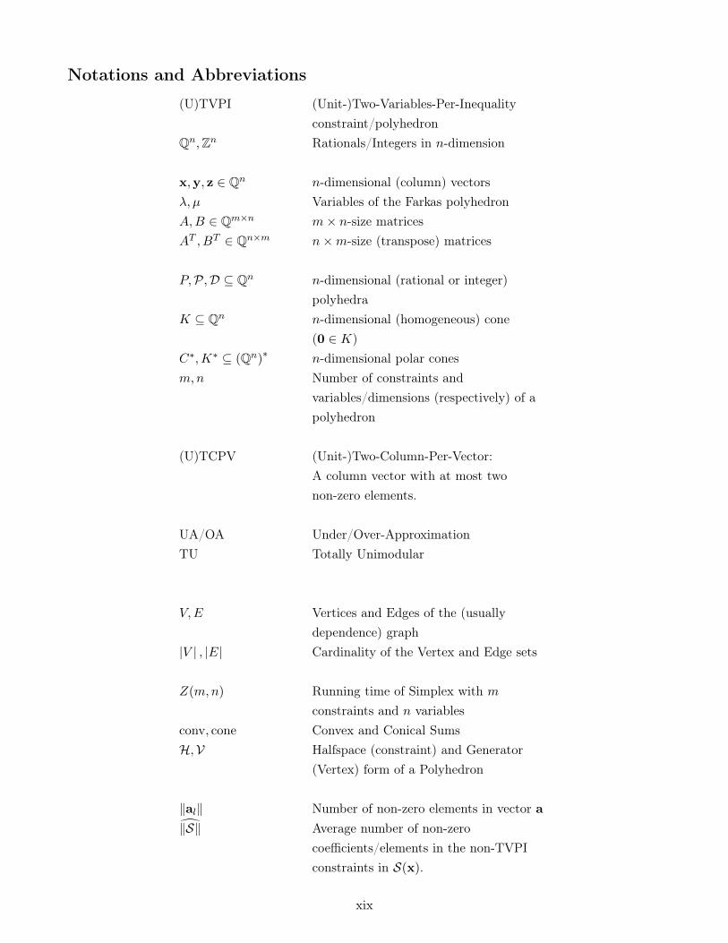
Notations and Abbreviations
(U)TVPI (Unit-)Two-Variables-Per-Inequalityconstraint/polyhedron
Qn,Zn Rationals/Integers in n-dimension
x,y, z ∈ Qn n-dimensional (column) vectorsλ, µ Variables of the Farkas polyhedronA,B ∈ Qm×n m× n-size matricesAT , BT ∈ Qn×m n×m-size (transpose) matrices
P,P,D ⊆ Qn n-dimensional (rational or integer)polyhedra
K ⊆ Qn n-dimensional (homogeneous) cone(0 ∈ K)
C∗,K∗ ⊆ (Qn)∗ n-dimensional polar conesm,n Number of constraints and
variables/dimensions (respectively) of apolyhedron
(U)TCPV (Unit-)Two-Column-Per-Vector:A column vector with at most twonon-zero elements.
UA/OA Under/Over-ApproximationTU Totally Unimodular
V,E Vertices and Edges of the (usuallydependence) graph
|V | , |E| Cardinality of the Vertex and Edge sets
Z(m,n) Running time of Simplex with mconstraints and n variables
conv, cone Convex and Conical SumsH,V Halfspace (constraint) and Generator
(Vertex) form of a Polyhedron
‖al‖ Number of non-zero elements in vector a‖S‖ Average number of non-zero
coefficients/elements in the non-TVPIconstraints in S(x).
xix

www.dedoimedo.com all rights reserved
xx

Chapter 1
Introduction
1.1 Motivation
Automatic compilation and translation of programs to newer architectures so that the program runs ef-ficiently exploiting all the resources of the machine has been an important problem since the advent ofprogramming languages. In particular, the recognition of the difference between a language which a pro-grammer “sees and thinks in” and a language which is particularly suited for the architecture has led to theunderstanding of a program transformations and the so called program optimizations. While the concept ofprogram transformations is well understood using a concept of equivalence between the input and outputprograms, the concept of optimizations is harder to define with many times such definition being archi-tecture dependent. With the modern day architectural challenges like decline of Moore’s law and the riseof multi-core machines—which have large computing powers equivalent to earlier era super-computers—which demand proper exploitation, defining optimizations has become a demanding, specialized and hardto solve task, even after decades of research.
The concept of these program optimizations has led to reasoning that iterative computation, usuallyexpressed as equivalents of for loops are best cases for optimization. Though many techniques havebeen introduced and evolved over decades, they have relatively been adhoc, lacking in formalism andcompleteness. The formal way to understand loop optimizations is now agreed upon to be a model termedas polyhedral compilation. This formalism, though extremely powerful to encode many interesting programtransformations, is quite costly for large input programs making the overall optimization process andhence the compiler unscalable. In this thesis we contribute to polyhedral compilation by introducing analgorithmic analysis and scalability driven approximations so that a precision vs. cost tradeoff can be madeby the optimizing compiler.
1.2 Key Concepts
Compilers. Compilation is a branch of computer science that is devoted to transforming a computerprogram in a source language to execute on a target architecture, with compilers being the associated sys-tems software. Though compilers usually perform several analysis and verifications on the input program,
1

www.dedoimedo.com all rights reserved
they are primarily used for the process of translation of a program from a source language—usually, likeC/C++/FORTRAN—to a prespecified target language. Sometimes, the source and target languages arethe same, in which case it is called a source-to-source compiler, with its output usually being linked to aregular out-of-the-box compiler. The process of compilation usually involves an intermediate language, oran intermediate form like an abstract syntax tree, which can represent the input program correctly.
Iterative regular computation. The seminal work of Karp Miller and Winograd [KMW67] introduceda model—called Systems of Uniform Recurrence Equations (SUREs)—which can be used to describe a setof regular computations as mathematical equations. Many key concepts in the reasoning of loop programscan be traced back to the above paper. The model of SUREs has been extended to Systems of AffineRecurrence Equations (SAREs) so that a restricted variety of for loop programs expressed in a languagelike C—with restrictions on the kinds of ranges of the iterator variables, the kinds of array accesses, thememory model of the variables etc.—can be represented, analyzed and transformed.
Loop program optimization. An optimization of an input program is understood to be its improve-ment on a pre-defined metric, like execution time, memory footprint, registers needed etc. Most compileroptimizations are inherently linked to a concrete measure of improvement, usually involving the archi-tectural characteristics. In earlier times, advanced compiler optimizations were reserved for supercomput-ers [Wol89]. But, with the widespread use of new powerful architectures, they have become a core part ofsystems research with many challenging problems to be solved. There have been many compiler optimiza-tions, like software pipelining, that have been designed to improve the performance of the output programwhen compared to the input program, but most of them bring about only a constant fold improvement. Ithas however been well recognized that optimization of iterative or regular computation expressed as loopprograms is the best way to bring about an asymptotic improvement in the running time of the input pro-gram. So, many individual optimizations, like loop distribution, permutation, unimodular transformations,shifting, etc. have been developed over the history of loop optimization. But, most of them are lacking informalism and completeness.
Polyhedral compilation. Polyhedral compilation is the compilation of loop programs using polyhedral(geometric) representations, and subsequent transformations obtained by rational and integer linear pro-gramming. It is generally accepted that the formalism in polyhedral compilation which is rooted in theabove cited Systems of Recurrence Equations work of Karp et al. is complete as well as being powerfulenough to encode many varieties of which are powerful affine transformations [DRV00]. One traditionalview is the polyhedral compiler should be designed to directly take in SAREs expressed in a high levellanguage, but the more practical view is that the input pieces of code—also called Static Control Parts ofa larger program (or SCoPs)—are usually expressed in a language similar to C, but have restrictions sothat equivalent SAREs could be derived from them. In this latter method, polyhedral compilation followsa three phase process. The first phase is a dependence analysis phase where the input program is analyzedand an equivalent polyhedral representation for it is constructed where the domains and dependences of theinput program are representable by rational parametrized polyhedra [Fea91]. This is followed by a schedul-
2

www.dedoimedo.com all rights reserved
ing or transformation finding phase [DRV00] where a proper optimization is found using the model definedby the architectural and other constraints. This is further followed by a code generation phase where theschedules are applied to the input program model to generate the transformed program [QRW00].
Affine scheduling. In polyhedral compilation, following the pioneering work of Feautrier [Fea92a,Fea92b] the constraints of the input program are translated to a new space defined by application of a LPduality transformation called affine form of Farkas lemma, and this new polyhedron (“Farkas polyhedron”)searched for the proper transfomations. Feautrier also defined affine scheduling and affine transformations,in which the transfomations are encoded by an affine function of the Farkas polyhedron. Affine transfor-mations not only have the advantage that searching for them simply involves solving a linear program, butalso they can be linked to a conceptually simple code generation scheme which leads to code that couldeven be directly translated to hardware if needed to. Because of the fact that affine scheduling is both ascheduling algorithm as well as a scheduling framework, the work of Feautrier’s model has been extended byGriebl et al. [GFG02]. The latter defined permutability conditions and subsequent space-time transforma-tional model named Forward Communications Only (FCO), which is particularly suited for tiling [GFL04].This FCO transformation has been re-defined with a cost function particularly amenable for multi-coremachines and implemented in the PLuTo source-to-source compiler by Bondhugula et al. [BHRS08]. Themodel of PLuTo has been very successful with variations of its algorithm having been implemened invarious compilers across industry: IBM’s XL, Reservoir Lab’s R-Stream, GCC’s GRAPHITE and morerecently in LLVM’s Polly compilers.
Code generation. After finding an optimizing transformation for the input program, the final step inpolyhedral compilation is polyhedral code generation, which is defined to be finding a scanning order for thetransformed program by touching each integer point in each of the domains exactly once, while respectingthe dependences between the statements. Though there have been many scheduling algorithms, and therewill be more in the coming times, the algorithm for scanning polyhedra by Quilleré et al. [QRW00],is the only one which can generate exact code. The above algorithm’s implementation in CLooG codegenerator [Bas04a] has comprehensively solved the code generation problem and is arguably the firstmodule that is put in when designing a new polyhedral compiler.
Sub-polyhedral compilation. The practical affine scheduling algorithms involve solving large (ratio-nal) linear programs whose size is dependent on the size of the input program. And, the polyhedral codegenerator algorithm involves polyhedral operations which take exponential time. Hence, both the schedul-ing and the code generation modules of polyhedral compilation are well understood to be asymptoticallyquite costly and hence unscalable when the input programs are large. The subject of this thesis is the intro-duction of sub-polyhedral compilation so that the asymptotic complexity of these two critical modules canbe reduced by using approximations of polyhedra or sub-polyhedra. The particular variety of sub-polyhedrathat we focus on is (Unit-)Two-Variables-Per-Inequality sub-polyhedra which are specialized or restrictedform of polyhedra, where each of the constraints could be only of the form axi + bxj ≤ c (±xi ± xj ≤ c).These varieties of polyhedra, because of the binary nature of their constraint relations, have the advantage
3
www.dedoimedo.com all rights reserved
that they can be represented using a graph theoretic encoding. Optimization and feasibility problems onsystems of constraints involving (U)TVPI polyhedra can be solved using problems like min-cost-flow andBellman-Ford algorithms, with the time complexity of these algorithms being asymptotically polynomialtime. Though these sub-polyhedral methods are powerful enough to encode interesting program trans-formations, they are lesser in power and precision than ones using general polyhedra, with a consequentgain in time complexity. So, use of sub-polyhedral compilation methods gives the compiler writer a uniqueprecision vs. cost tradeoff, which she can factor in while designing polyhedral scheduling and polyhedralcode-generation problems.
1.3 Overview of this Thesis
This thesis is organized as follows.
In Chapter 2, we first give some basics of polyhedral compilation and affine scheduling. We then showa theoretical analysis of the asymptotic complexity of the unscalability problem in scheduling, followedby an empirical measurement of the affine scheduling methods currently implemented in PLuTo; we showthat they do not scale for large versions of typical input programs.
In Chapter 3, we study various classes of sub-polyhedra, the time complexities of their operators andpredicates, along with their use in static analysis. After reviewing the many varieties of sub-polyhedrathat have been used by the static analysis community for abstract interpretation purposes, and the com-plexity theory community for algorithmic improvements, we focus on (Unit-)Two-Variables-Per-Inequalitypolyhedra; namely, ones with constraints of the form axi + bxj ≤ c; a, b, c ∈ Q (and ±xi ± xj ≤ c; c ∈ Qrespectively). After the above study of sub-polyhedra purely on an asymptotic analysis purposes, in Chap-ter 4, we study whether any approximations have already been used in polyhedral scheduling. Afterunderstanding the limitations of some of the major varieties of polyhedral approximations, we introducea new variety of affine scheduling: polyhedral scheduling using (U)TVPI sub-polyhedra.
The above scheduling technique needs under-approximation algorithms, and hence, the next two chap-ters focus on developing new algorithms which under-approximate a general polyhedron into (U)TVPIsub-polyhedra. To do this, in Chapter 5 we introduce a duality based framework that is particularly suitedfor our purposes. In Chapter 6, we design Under-Approximation algorithms. These algorithms run in poly-nomial time and provide a method by which the UA algorithms could be applied on a per-dependencebasis, or on the overall Farkas polyhedron.
In Chapter 7, we present experimental results showing the effectiveness of our mentioned methodsby implementing them in PLuTo, a state-of-the-art compiler for tiling and parallelization purposes. Thisexperimentation is based both on a polyhedral theoretical sense as well as from the perspective of compi-lation, namely, feasibility study of the above suggested under-approximation algorithms, improvements inthe execution time of the scheduler, and execution time of the generated code.
In Chapter 8, we study various loop optimization applications that use the above UA framework to im-prove their worst-case asymptotic complexity. The complexities of the original problems range from weaklypolynomial time to NP-Complete, while the complexities of the algorithms that we suggest are always of
4
www.dedoimedo.com all rights reserved
fixed weakly or strongly polynomial time. In Chapter 9, we introduce sub-polyhedral code-generation; apreliminary approach to see how the lower complexities of (U)TVPI sub-polyhedra can be used to obtainbetter worst-case bounds for polyhedral code generation, albeit for loss of precision in the form of reductionof quality of the generated code, and increased control overhead.
In Chapter 10, we provide some conclusions and perspectives.The problems being solved in this thesis, the approaches and results by which it was influenced, and
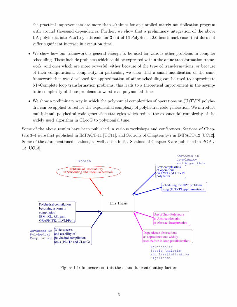
the contributing factors therein, are briefly summarized in Figure 1.1.
1.4 Our Contributions
One important goal during this thesis was to introduce the scalability analysis of parallelization of loopprograms that is firmly rooted in complexity theoretic asymptotic analysis. In particular, our contributionsare theoretical and algorithmic and are of practical interest as well. Our work takes in ideas from complexitytheoretic community, static analysis community, and the polyhedral loop optimization community. Hereare our contributions:
• We show, both theoretically and empirically, that the current methods used in polyhedral compi-lation are unscalable. The above leads to proposal of sub-polyhedral compilation strategies. Theyintroduce the concept of trading precision for execution time in a complexity guided manner, witha compilation-time scalability motivation.
• Of the many sub-polyhedra used in static analysis, we show that Two-Variable-Per-Inequality (TVPI)and Unit-Two-Variable-Per-Inequality (UTVPI) sub-polyhedra can provide good alternatives to beused in polyhedral scheduling, limiting its worst-case complexity. We show that state-of-the-artparallelization and affine scheduling heuristics such as PLuTo can be adapted to (U)TVPI sub-polyhedra, thereby reducing their algorithmic complexity. We propose two alternative algorithms—either with a direct Under-Approximation of all the feasible schedules, or as an intersection ofUnder-Approximations of Farkas polyhedra per each dependence edge—which can be used to solvefeasibility problems of large polyhedra arising in affine scheduling.
• Using elementary polyhedral concepts, we present a simple and powerful framework (an approxi-mation scheme) which can be used for designing Under-Approximation (UA) algorithms of generalconvex polyhedra, linearizing the UA problem. Using the above framework, we present five sim-ple algorithms that under-approximate a general polyhedra expressed in constraint representation(H-form) into (U)TVPI sub-polyhedra.
• We evaluate these methods by integrating them into the PLuTo polyhedral compiler. We show thatfor 29 out of 45 Farkas-polyhedra arising from PolyBench 2.0, the (U)TVPI-UAs proposed above areprecise enough to preserve feasibility. We show that our approximations when solved with a Bellman-Ford algorithm show theoretically asymptotic, and practically considerable improvement in runningtime over a well established Simplex implementation; more particularly, the theoretical improvementsare a reduction from |V |5 to |V |3, where |V | is the number of statements in the input program, while
5
www.dedoimedo.com all rights reserved
the practical improvements are more than 40 times for an unrolled matrix multiplication programwith around thousand dependences. Further, we show that a preliminary integration of the aboveUA polyhedra into PLuTo yields code for 3 out of 16 PolyBench 2.0 benchmark cases that does notsuffer significant increase in execution time.
• We show how our framework is general enough to be used for various other problems in compilerscheduling. These include problems which could be expressed within the affine transformation frame-work, and ones which are more powerful: either because of the type of transformations, or becauseof their computational complexity. In particular, we show that a small modification of the sameframework that was developed for approximation of affine scheduling can be used to approximateNP-Complete loop transformation problems; this leads to a theoretical improvement in the asymp-totic complexity of these problems to worst-case polynomial time.
• We show a preliminary way in which the polynomial complexities of operations on (U)TVPI polyhe-dra can be applied to reduce the exponential complexiy of polyhedral code generation. We introducemultiple sub-polyhedral code generation strategies which reduce the exponential complexity of thewidely used algorithm in CLooG to polynomial time.
Some of the above results have been published in various workshops and conferences. Sections of Chap-ters 3–4 were first published in IMPACT-11 [UC11], and Sections of Chapters 5–7 in IMPACT-12 [UC12].Some of the aforementioned sections, as well as the initial Sections of Chapter 8 are published in POPL-13 [UC13].
polyhedra
This Thesis
Scheduling for NPC problems
using (U)TVPI approximations
Problems of unscalabilityin Scheduling and Code−Generation
Polyhedral compilation
becoming a norm in
compilation
IBM−XL, RStream,
GRAPHITE, LLVM/Polly
Wide success
and usability of
polyhedral compilation
tools (PLuTo and CLooG)
Use of Sub−Polyhedra
as Abstract domain
in Abstract interpretation
Dependence abstractions
as approximations widely
used before in loop parallelization
Advances in
Polyhedral
Compilation
Advances in
Complexity
and Algorithms
Advances in
Static Analysis
and Parallelization
Algorithms
Problem
Low complexitiesof operationson TVPI and UTVPI
Figure 1.1: Influences on this thesis and its contributing factors
6

Chapter 2
Polyhedral Scheduling and the ScalabilityChallenge
In this chapter, we summarize polyhedral compilation, affine scheduling, and provide a motivation forsolving the scalability problem in it.
2.1 Introduction
Affine scheduling [DRV00] now is a part and parcel of many compilers which aspire to compile efficientlyfor parallel architectures (GCC’s GRAPHITE, IBM’s XL, Reservoir Lab’s R-Stream, LLVM’s Polly). Theseminal work of Feautrier [Fea92a] opened the avenue of constraint-based affine transformation methods,building on the affine form of the Farkas lemma. This approach has been refined, extended and applied inmany directions. To cite only two recent achievements at the two extremes of the complexity spectrum:the tiling-centric PLuTo algorithm of Bondhugula et al. [BHRS08] extending the Forward Communica-tion Only (FCO) principle of Griebl et al. [GFG02, GFL04] for coarse-grain parallelization, and thecomplete, convex characterization of Vasilache [Vas07] and decoupled exploration heuristic of Pouchetet al. [PBB+11]. Much progress has been made in the understanding of the theoretical and practicalcomplexity of polyhedral compilation problems. Nevertheless, when considering multidimensional affinetransformations, none of these are strongly polynomial in the size of the program. The lowest complexityheuristics such as PLuTo are reducible to linear programming, which is only weakly polynomial, its tradi-tional Simplex implementation being associated with large memory requirements and having a worst-caseexponential complexity.
In this chapter, we make a case for solving the scalability problem in polyhedral scheduling. First, inSection 2.2, we give a very brief and quick introduction of affine scheduling. This is followed in Section 2.3where a case is made from different perspectives for solving the scalability problem in affine scheduling.Then in Section 2.4, we conclude this chapter giving a brief overview of the approaches that are developedin the next chapters.
7
www.dedoimedo.com all rights reserved
2.2 Affine Scheduling: A Quick Introduction
In this section we quickly introduce some of the terms needed for this dissertation. As there are resourceslike the book by Darte et al. [DRV00] which do a good introduction to the highly specialized topic ofpolyhedral scheduling, we will only recall some essential notations and results about polyhedral compilationand in particular, affine scheduling.
Mathematical preliminaries. The mathematics needed for affine scheduling is linear programming,convexity and duality [Sch86, Zie06]. An affine transformation is an image function of the type f(x) =
{y |y = Ax + b}. A polyhedron is a set of rational points enclosed by affine inequalities involving the vari-ables x: P = {x ∈ Zn |Ax ≤ b}, while a parametric polyhedron Py = {x ∈ Zn |Ax +My ≤ b} is definedto be a set of rational points enclosed by affine inequalities involving the variables x and additional sym-bolic constants (“parameters”) y. A polyhedron can be in either of its representations, the constraint form(H-form) and its generator form (V-form). The conversion from one form to the other can be performedby the Chernikova algorithm [Ver92], which is available in libraries like PolyLib [Wil93].
Input programs. The input programs for polyhedral compilation are called Static Control Parts (SCoPs).A SCoP [Fea91] in a program like C can have only for loops along with if conditionals, where the iteratorsof the former and conditionals of the latter define convex shapes, and are defined as affine functions of theouter loop indices and the symbolic constants (“parameters”). Also, the array variables have indices whichcan be described using affine functions. For these reasons, SCoPs have also been called as Affine ControlLoops (ACLs) in literature. There are some other assumptions about SCoPs, like the array variables aremapped to linear memories that do not intersect with each other and the index variables are unaliasedwith each other, but such detection is left to the static analyzer of the compiler, and not to the polyhe-dral compiler itself. The more powerful the static analyzer is, along with its modules like alias and pointeranalysis, the larger and more numerous are the SCoPs which are input to the polyhedral compiler. In somesource-to-source compilers, SCoPs are marked by a set of pragmas. SCoPs may seem to be pieces of codeof a restricted variety, but are powerful enough to encode many interesting applications, like dense matrixapplications, linear algebra applications or stencil computations. In fact they are Turing complete [SQ93]and equivalent Systems of Affine Recurrence Equations (SAREs) can be derived from them.
Dependences and dependence analysis. In a SCoP, a dependence is said to exist between two mem-ory accesses if one of the accesses is a write. Data dependence analysis is a well-formulated and well-solvedproblem; Banerjee’s book [Ban92], and Zima and Chapman [ZC90] are good references. Computationally,it involves solving finite number of parametric integer linear programs with tools like PIP [Fea88] or byOmega [Pug91]. Polyhedral dependence analysis is the primary means of analyzing the input SCoPs andreturning a dependence graph whose edges are annotated by parametrized polyhedra which indicate theregions of dependence between the two variables or statements in context.
8
www.dedoimedo.com all rights reserved
Dependence graph. The output of a dependence analysis, and input to any polyhedral schedulingalgorithm is a polyhedral dependence graph G, and is defined to be a multi-graph G = (V,E), whereV is the set of statements, and E is the set of dependence edges. Both kinds of entities are annotatedby parametrized rational polyhedra; the nodes v ∈ V are by rational polyhedral approximations of theiteration domains (or plainly domains) Pv and the edges e ∈ E by dependence polyhedra De. Each ofthe constraints of Pv and De is affine and involves (I,N) where vectors I and N are the iteration andparameter vectors, respectively.
Dependence satisfaction. The primary constraints inherent to the program that have to be satisfiedare the dependence edges as formulated by Feautrier [Fea92a]. The above, usually called strong satisfactionof dependences, is simple to formulate in a LP formulation, but may seem overly restrictive because ofthe reduction of the number of interesting transformations. A related notion is called weak satisfactionof dependences arises from the lexicographic positivity nature of dependences and from the intuitionthat a dependence satisfied in a lower dimension may be enough to leave as unconstrained the dependencesatisfaction of the higher dimensions. This latter notion leads to more freedom by exposing more interestingtransformations, though searching for the proper schedules becomes a hard combinatorial problem becausethe question “which dimension of which dependence is to be satisfied at what level?” needs to be answered.
Affine transformations and Farkas lemma. An affine transformations finds an affine function in(I,N) to transform the input SCoP. These have also been called affine mappings, space-time mappings,and even plainly affine schedules. Because of the fact that every computable SARE, and hence every SCoPin a language like C, has a multi-dimensional affine schedule [Fea92b]—with the unit schedule being a trivialexample of multi-dimensional schedule—these transformations are extremely powerful. They are practicalas well, as most common and useful loop transformations can be expressed as affine transformations;though common simple examples are single loop nest transformations like reversal, skewing, shifting,unimodular transformations etc., the result on complete convex characterization of semantic preservingtransformations by Vasilache [Vas07] proves their generality. Though these transformations happen in theinput space, with the (I,N) vector as variables, the transformations are searched for in a transformed affinespace obtained by application of affine form of Farkas lemma. All the affine transformations in polyhedralcompilation could be said to come under the framework of affine scheduling defined by Feautrier in hisclassic works [Fea92a, Fea92b]. The most popular of these are the latency minimization algorithm byFeautrier [Fea92a] and the Forward Communications Only space-time mapping of Griebl et al. [GFG02,GFL04] and its extension by Bondhugula et al. [BHRS08]. This latter algorithm is the basic engine inPLuTo.
In Feautrier’s algorithm [Fea92a], the input dependence constraints are converted into a per-dependenceedge polyhedron Pe(µ, λ), with µ-variables being the Farkas multipliers that come from domain constraintsand λ-variables being the Farkas multipliers that come from dependence constraints. This conversion isdone by application of the affine form of the Farkas lemma [Sch86, Corollary 7.1h] given as:
9

www.dedoimedo.com all rights reserved
Lemma 2.2 [Affine Form of Farkas’s Lemma]. Let D be a nonempty polyhedron defined by p
inequalities akx + bk ≥ 0, for any k ∈ {1, . . . , p}. An affine form Φ is non-negative over D if and only if itis a non-negative affine combination of the affine forms used to define D, meaning:
Φ(x) ≡ λ0 +
p∑k=1
λk(akx + bk); ∀k ∈ [0, p]λk ≥ 0
The nonnegative values λk are called Farkas’s multipliers.Feautrier’s scheduler uses the above version of Farkas lemma so as to linearize the polyhedra in the
presence of iterator vectors and parameter vectors. In the per-edge Farkas polyhedron Pe(µ, λ), both ofthe newly created λ and µ variables are called the Farkas multipliers. By putting together all the per-edgeFarkas polyhedra, one obtains an overall Farkas polyhedron P = ∩e∈EPe, which is amenable to LinearProgramming. Any rational point that satisfies P is considered a valid schedule. Hence, even Fourier-Motzkin elimination could be used to obtain a feasible point.
Two models of affine scheduling. The above application of the Farkas lemma results in all the con-straints in the Feautrier’s scheduler, with some additional variables to model the strong/strict satisfactionof dependences at a given dimension of the affine schedule. In PLuTo, a different but conceptually similarmethod results in a majority of dependence constraints of the same form as Feautrier’s.
2.3 Motivation: Unscalability in Affine Scheduling
Before we attempt to solve it, we first attempt to define the problem of scalability.
2.3.1 Introduction: A definition of unscalability
Difficulties of defining the problem. The problem of scalability is difficult to define because of thefollowing reasons:
a. Relying purely on asymptotic analysis may provide only a partial picture of the usefulness of theparticular algorithm. The asymptotic analysis says that an algorithm with worst-case complexityO(|V |5) is cheaper than one with O(|V |6) worst-case complexity, while for small-size practical inputs,the reverse may be true; an algorithm with |V |6 complexity may be better than one with 106|V |5complexity. Furthermore, algorithmic and data-structure improvements that take O(|V | log∗ |V |) orO(|V |α(|V |)) worst-case time have remained as theoretical curiosities, while theoretically slower onesthat instead take |V | log |V | have remained as the most widely used ones.
b. Algorithms which rely on constructing huge size tableaus have limited scope. In spite of memorybecoming cheaper by drastic amounts, the amount of memory that a compilers can devote to one ofits phases is limited; the problem is exacerbated for JIT compilers.
c. Use of standard tools like LP-solvers, ILP-solvers and SAT-solvers does not solve the problem. This isbecause, many times, the complexity of the tools does not match that of the algorithm. Furthermore,
10

www.dedoimedo.com all rights reserved
many of these tools have heuristics that are tuned for some applications which may not be useful forpolyhedral compilation applications.
In spite of the apparent theoretical nature of the above questions, they have to be answered becauseof the way they manifest in practical polyhedral compilation.
Beginning to solve the problem. Our analysis begins with opening the boxes of the transformationsalong with their tools and measuring the precise complexities as parametrized by input sizes: for example,the number of statements |V | and dependence edges |E| in the input SCoP, the maximum depth d of theinput loop-nest etc. This is despite the fact that they rely on well written and well used tools like PIP,PolyLib, etc.
View of this dissertation. The view taken by this dissertation is to prefer asymptotic time com-plexity analysis as the primary means of measuring the scalability or unscalability of an algorithm, andto evaluate different competing algorithms. By this measure, any solution which uses an NP-Completeformulation, would clearly be unscalable. Even among polynomial algorithms, we prefer algorithms withstrongly polynomial time complexity, rather than ones which have weakly polynomial time complexity.
Furthermore, will also rely on memory complexity analysis as the secondary means of measuringscalability. Algorithms which rely on construction of huge-size tableau’s—like simplex does—are likely tobe heavy in compilation frameworks, like for JIT compilation.
The above leaves linear and quadratic time complexities as scalable complexities, which should be theeventual and perhaps ideal goal. Even after after all these, we will measure how the algorithms performsfor practical inputs.
Overview of this section. In this section, we show an example of unscalability of current affine schedul-ing methods in an empirical sense using PLuTo, followed by a theoretical evaluation. First in Section 2.3.2,we do an experimental evaluation of affine scheduling. Then in Section 2.3.3, we see the practical ways inwhich the unscalability problem can arise in practical inputs. Then, in Section 2.3.4, we see some empiricalcharacteristics of the above LP programs. Finally, in Section 2.3.5, making some reasonable estimates, weestimate the complexity of affine scheduling.
2.3.2 Unscalability in affine scheduling: an experimental evaluation
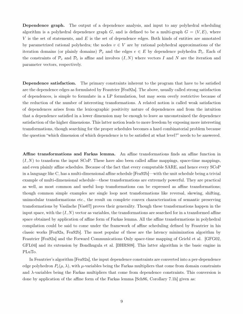
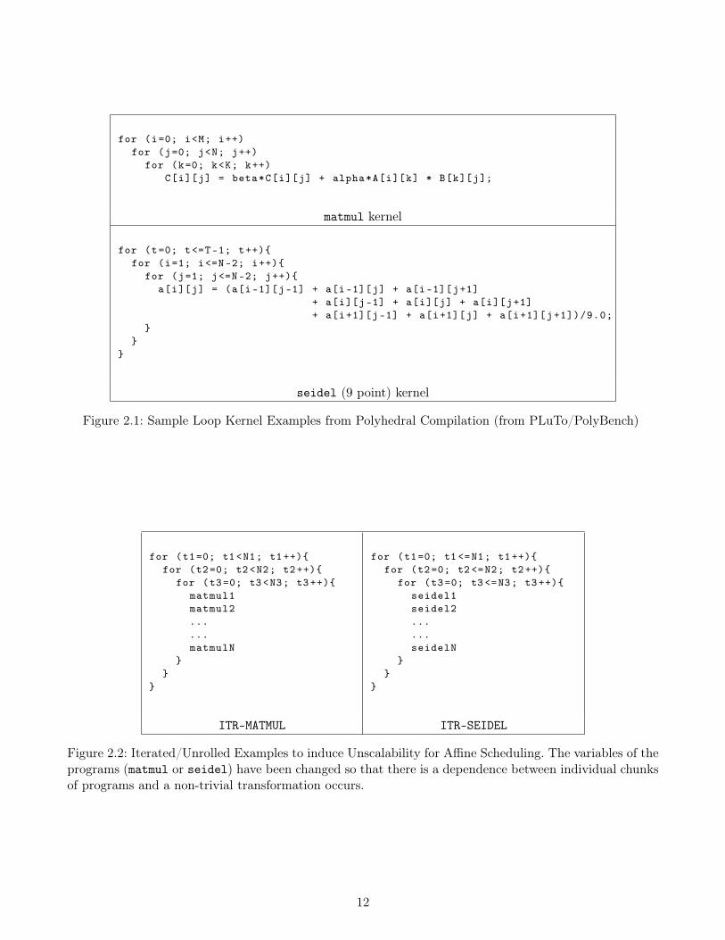
Input programs. We began with two typical kernels matmul and seidel of PolyBench [PB+] as shownin Figure 2.1, and artificially unrolled them by a variable number of times so as to increase the numberof dependences in the loop nests. As shown in Figure 2.2, we have also enclosed the unrolled loops in twoor three “time loops”, mimicking the behavior of a scientific computing kernel. The above transformationsinduce thousands of dependences in the input programs—up to 4000 dependences for matmul, and upto 7000 dependences for seidel—and thereby make the scheduler solve large size linear programs. In asense, the two programs that have been selected form the extreme end of affine transformations; matmulhas only affine dependences, while seidel has only uniform dependences. This difference is crucial because
11
www.dedoimedo.com all rights reserved
for (i=0; i<M; i++)for (j=0; j<N; j++)
for (k=0; k<K; k++)C[i][j] = beta*C[i][j] + alpha*A[i][k] * B[k][j];
matmul kernel
for (t=0; t<=T-1; t++){for (i=1; i<=N-2; i++){
for (j=1; j<=N-2; j++){a[i][j] = (a[i-1][j-1] + a[i-1][j] + a[i-1][j+1]
+ a[i][j-1] + a[i][j] + a[i][j+1]+ a[i+1][j-1] + a[i+1][j] + a[i+1][j+1])/9.0;
}}
}
seidel (9 point) kernel
Figure 2.1: Sample Loop Kernel Examples from Polyhedral Compilation (from PLuTo/PolyBench)
for (t1=0; t1 <N1; t1++){for (t2=0; t2 <N2; t2++){
for (t3=0; t3 <N3; t3++){matmul1matmul2......matmulN
}}
}
for (t1=0; t1 <=N1; t1++){for (t2=0; t2 <=N2; t2++){
for (t3=0; t3 <=N3; t3++){seidel1seidel2......seidelN
}}
}
ITR-MATMUL ITR-SEIDEL
Figure 2.2: Iterated/Unrolled Examples to induce Unscalability for Affine Scheduling. The variables of theprograms (matmul or seidel) have been changed so that there is a dependence between individual chunksof programs and a non-trivial transformation occurs.
12

www.dedoimedo.com all rights reserved
0 1000 2000 3000 4000 5000 6000 7000
020
40
60
80
10
0
Auto−Trans Time taken (Seconds) vs. Number of Dependences
Dependences
Tim
e taken
(S
eco
nds)
Unrolled SCoPs
Seidel Matmul
Figure 2.3: Unscalability for Large Loop Programs
the programs with affine dependences may induce Farkas systems which are more complex than the onewith uniform dependences, thereby making the simplex algorithm in the LP solver of PIP [Fea88] convergewith different rates, namely higher rate for the ones with affine dependences.
Compilation times. For measuring the execution time of the scheduler, we focussed on auto_transform
function of PLuTo, which encodes its top-level automatic transformation search engine. The above functionis preceeded by a call to the clan_scop_extract function which does dependence analysis of the inputpieces of code, and succeeded by the pluto_codegen function which does the code-generation by makinga call to the popular code-generator CLooG. More particularly, the above function auto_transform iter-atively constructs the Farkas polyhedra according to its formulation of the FCO algorithm, makes a callto PIP’s linear programming solver to find a lexmin of the Farkas systems, and interprets the resultantsolution to obtain permutable hyperplanes.
The execution times of auto_transform are shown in Figure 2.3, with matmul in blue (crosses) andseidel in red (circles). We also measured independently the time taken in execution of rest of the modulesof PLuTo—in particular, the dependence analysis and code generation phases—and found that they tooksignificantly less time than the above measured times.
Rise of the curves. Using linear regression tools from The R Project for Statistical Computing [R], wechecked that the execution times of auto_transform increases in a quintic complexity: |V |5, where |V | is
13

www.dedoimedo.com all rights reserved
the number of statements in the system. This is the high complexity that polyhedral compilation has topay for using LP based techniques.
Unscalability in different modules of affine scheduling. Within affine scheduling itself, there arevarious algorithms like Farkas multipliers elimination by gaussian elimination and a limited preprocessingwith Fourier-Motzkin elimination. Even though these could be costly in themselves, these are not majorsources of unscalability. This is primarily because they can be done on a per-dependence basis and theper-dependence Farkas polyhedra are considerably smaller to afford high-complexity algorithms.
Unscalability in different modules of polyhedral compiler. From the curves in Figure 2.3, itis clear that there is a strong case of solving the scalability problem for affine scheduling in polyhedralcompilers using affine scheduling. From these experiments, we have also observed that dependence analysisand code generation are not major sources of unscalability when compared to affine scheduling.
The former is not much surprising since the dependence polyhedra, being mainly per-dependenceentities, are considerably smaller than the overall Farkas polyhedra. This will be empirically shown in thisdissertation in Section 7.2 on page 90. Furthermore, dependence analysis is a relatively one-time processwhose cost does not vary much asymptotically with the input program size, with its cost being limited toO(|E|) number of linear programs whose size is bounded.
The latter is a little surprising because polyhedral code generation has its own scalability problemsdefinitely arising from use of exponential time algorithms and polyhedral libraries with exponential com-plexity. But, it can only be reconciled that for these particular examples, the scalability problem in codegeneration is not manifested, and there exist other examples for which there is a perceptible unscalabilityproblem, for example like programs which do multi-level tiling. The aspect of scalability in code-generationis studied further in this dissertation in Chapter 9 on page 127.
2.3.3 Practical causes of unscalability
It may seem that the above unrolling based method is an artificial way to induce unscalability, with inliningbeing a better candidate for the same in real world benchmarks. Also, in current benchmarks for loop nestoptimization—like the PolyBench 2.0 [PB+]—the range of number of dependences is in tens, and it canarguably be said that presently there exists no scalability problem like in the above artificial examples.
Unrolling vs. inlining. While unrolling is much simpler to simulate, limitations of the research proto-type infrastructures we have used—unlike more powerful ones like PIPS [PIP]—do not provide a platformto study the asymptotic time complexity associated with code size increases associated with inlining.Hence, the above examples could only be taken as representatives of the unscalability problem. But itshould also be remembered that when discussing the solution time with respect to the input code sizeincrease, the number of constraints in the overall LP problem is linear in the number of dependences inthe input code. So, a method like the above which gives a representative sample to increase the size of theLP program is not a limitation.
14
www.dedoimedo.com all rights reserved
Longer source codes. Longer source codes in the input programs, which lead to longer SCoPs andhence larger LP programs that the affine scheduler has to solve, could arise not just from inlining orunrolling. They could arise from difficult and more expressive source languages. The current input languageof PLuTo is a variation of C, which does not have powerful features like templates of C++. Polyhedralcompilers will soon face such large problems when the Front End of polyhedral compilers is improved. And,aggressive interprocedural optimization, domain-specific program generation along with the iteraction ofC++ program features like templates with inlining could exponentially increase the size of SCoPs. Also,sources in medium/low-level languages and preceded by more powerful static analysis like alias/pointeranalysis as a part of compiler framework like in GCC-GRAPHITE [TCE+10] make these issues a verypossible reality.
Expanding the definition of SCoPs. Longer SCoPs could also arise from the removal of restrictionson the definition of SCoPs in the input program and thereby increase the range of programs that couldcome under the category of affine analysis. In this trait are the works of Griebl et al. [Gri96, GL94] on while
loop parallelization, and analyses like Maximal Static Expansion (MSE) by Barthou et al. [BCC00] whoprovide an expansion framework for general (possibly non-affine) data structures. In the same categoryis the work of Benabderrahmane et al. [BPCB10] who add more categories of programs for polyhedralanalysis, by removing the affinity limitation in the input SCoPs by conservatively approximating thenon-affine domains, and by converting control dependences into data dependences.
JIT compilation. In addition, there could be a restriction of the time limit in just-in-time compilersthat would further exacerbate the scalability problem. Just-In-Time (JIT) polyhedral compiler of LLVMcalled Polly [GGL12] is such an example which has a scheduler, which is very similar to the one in PLuTo.
Existing limitations on unscalability. Also, industrial compilers like IBM’s XL, and Reservoir’s R-Stream compiler have schedulers very similar to PLuTo, and the IBM-XL compiler is known to limit thecompilation time of kernels of using its polyhedral compilation module to 10 seconds. One can see theparticular time limit being crossed by PLuTo in the above plot for both the examples. For an initial rangeestimate, our experiments indicate that the 10 second compilation limit could be crossed for around 1000
dependences which is possible with the above mentioned reasons.In the following, we aim for lower complexity feasibility and optimization algorithms, with worst-
case strongly polynomial bounds, and closer to n2 time complexity for large-scale and/or just-in-timecompilation applications.
2.3.4 LP program characteristics
So as to understand the empirical complexity a little better, in Figure 2.4, we plot the characteristics ofthe ITR-MATMUL, using the pairs function of R [R].
We denote |V | to be the number of statements in the input dependence graph, |E| to be the numberof dependences, m to be the number of constraints in the LP overall formulation, and τ to be the time
15
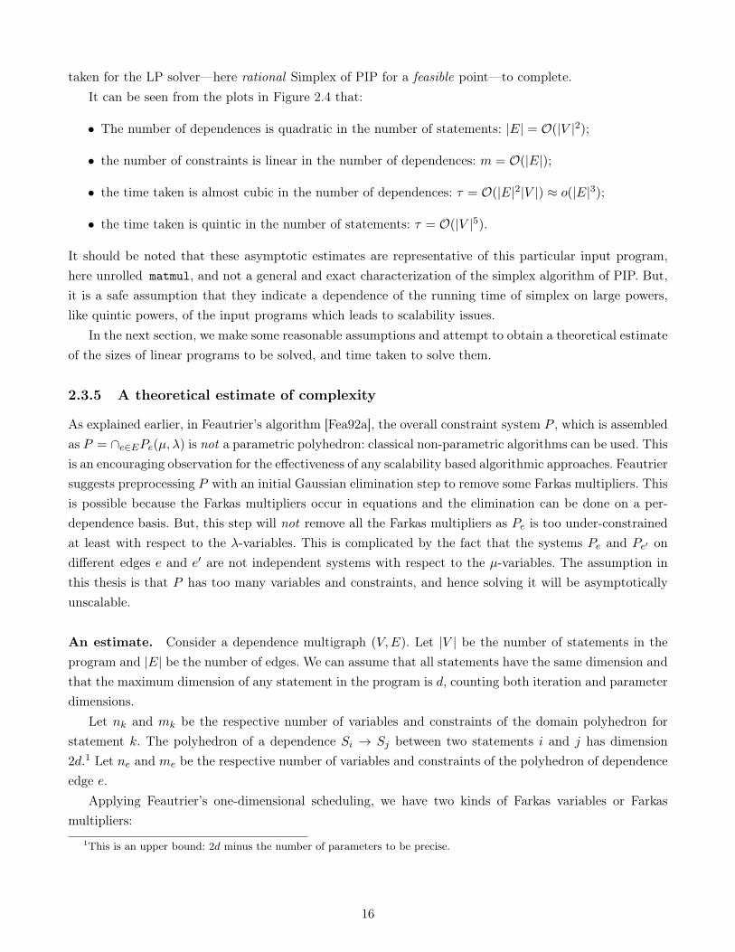
www.dedoimedo.com all rights reserved
taken for the LP solver—here rational Simplex of PIP for a feasible point—to complete.It can be seen from the plots in Figure 2.4 that:
• The number of dependences is quadratic in the number of statements: |E| = O(|V |2);
• the number of constraints is linear in the number of dependences: m = O(|E|);
• the time taken is almost cubic in the number of dependences: τ = O(|E|2|V |) ≈ o(|E|3);
• the time taken is quintic in the number of statements: τ = O(|V |5).
It should be noted that these asymptotic estimates are representative of this particular input program,here unrolled matmul, and not a general and exact characterization of the simplex algorithm of PIP. But,it is a safe assumption that they indicate a dependence of the running time of simplex on large powers,like quintic powers, of the input programs which leads to scalability issues.
In the next section, we make some reasonable assumptions and attempt to obtain a theoretical estimateof the sizes of linear programs to be solved, and time taken to solve them.
2.3.5 A theoretical estimate of complexity
As explained earlier, in Feautrier’s algorithm [Fea92a], the overall constraint system P , which is assembledas P = ∩e∈EPe(µ, λ) is not a parametric polyhedron: classical non-parametric algorithms can be used. Thisis an encouraging observation for the effectiveness of any scalability based algorithmic approaches. Feautriersuggests preprocessing P with an initial Gaussian elimination step to remove some Farkas multipliers. Thisis possible because the Farkas multipliers occur in equations and the elimination can be done on a per-dependence basis. But, this step will not remove all the Farkas multipliers as Pe is too under-constrainedat least with respect to the λ-variables. This is complicated by the fact that the systems Pe and Pe′ ondifferent edges e and e′ are not independent systems with respect to the µ-variables. The assumption inthis thesis is that P has too many variables and constraints, and hence solving it will be asymptoticallyunscalable.
An estimate. Consider a dependence multigraph (V,E). Let |V | be the number of statements in theprogram and |E| be the number of edges. We can assume that all statements have the same dimension andthat the maximum dimension of any statement in the program is d, counting both iteration and parameterdimensions.
Let nk and mk be the respective number of variables and constraints of the domain polyhedron forstatement k. The polyhedron of a dependence Si → Sj between two statements i and j has dimension2d.1 Let ne and me be the respective number of variables and constraints of the polyhedron of dependenceedge e.
Applying Feautrier’s one-dimensional scheduling, we have two kinds of Farkas variables or Farkasmultipliers:
1This is an upper bound: 2d minus the number of parameters to be precise.
16

www.dedoimedo.com all rights reserved
STMTS
0 1000 2000 3000 4000 0 1 2 3
05
10
15
20
25
01
00
02
00
03
00
04
000
DEPS
PIPCONSTR
02
000
400
06
00
08
000
0 5 10 15 20 25
01
23
0 2000 4000 6000 8000
PIPTIME
Figure 2.4: Characteristics of LP programs of ITR-MATMUL for Unscalability: #Statements (STMTS) vs.#Dependences (DEPS) vs. #Constraints (CONSTR) vs. Time Taken per PIP call (PIPTIME)
17
www.dedoimedo.com all rights reserved
• one λ variable per dependence and per dependence constraint. So, the total number of λ variables is2d∑
e∈Eme = 2d|E|mE , where mE is the average number of constraints per dependence polyhedron;
• one µ variable per statement and per domain constraint. So the total number of µ variables isd∑
k∈V mk = d|V |mV , where mV is the average number of constraints per domain polyhedron.
Also, the total number of constraints in the complete system is d|E|.The above estimates lead to a linear programming problem with d|E| constraints and around 2d|E|mE+
d|V |mV variables. As suggested by Feautrier [Fea92a], we can assume that a gaussian elimination stepruns as a preprocessing step to remove λ-variables which occur only in equalities, and is able to remove asignificant number of them, making the number of variables as d|V |mV . This elimination step would beinexpensive as it can run on a per-dependence edge basis. We can also validly assume that mV is a verysmall bounded value, making the number of variables in the overall system to be d|V |.
Assuming a usual complexity of linear programming solved with a normal simplex algorithm (the bestalgorithm for state-of-the-art Farkas-based methods)2, this brings the total complexity of the schedulingalgorithm to order of:
(d|V |+ d|E|) · d|E| · d|V | ≈ d3|E|2|V | = O(|E|2|V |)
Assuming that the dependence graph is a complete graph, we have |E| ≈ |V |2 which makes the abovecomplexity to as O(|V |5). This complexity could be worse when the dependence graph is a more densemulti-graph, or in presence of piecewise-affine dependence relations (e.g., in some cases after array data-flow analysis).
The above complexities are clearly not scalable. Analyzing the PLuTo algorithm leads to a similar com-putation and the same non-scalability result. Practical evidence shows that it scales well on all benchmarksconsidered so far. But no benchmark with thousands of loops and statements has been processed either,which will no doubt happen with three-address code representations [TCE+10] and extensions to irregular,data-dependent control flow [BPCB10]. Considering Feautrier multi-dimensional scheduling [Fea92b] onlymakes things worse, as it could involve solving a mixed-integer linear programming problem.
2.4 Conclusion and Brief Overview of Our Approaches
Conclusion. In this chapter, after a quick summary of polyhedral scheduling, we showed using boththeoretical and empirical ways that existing methods result in an LP problem of size m× n ≈ (d · |E|)×(d·|V |), where d is the mean depth of the loop nests. Assuming a usual simplex method—whose complexitywill be detailed further in Section 3.3.1 on page 28—for solving systems with bounded d leads to a closeto O(d3|E|2|V |) ≈ O(d3|V |5) ≈ O(|V |5) asymptotic complexity (not counting the bit-size complexity, andassuming |E| = O(|V |2)), leading to unscalability problems. The estimates focus on Feautrier’s methodsbut are general enough to be extended to any affine scheduling methods like the FCO implementation inPLuTo.
2This algorithmic analysis will be further developed in Section 3.3.1 on page 28.
18
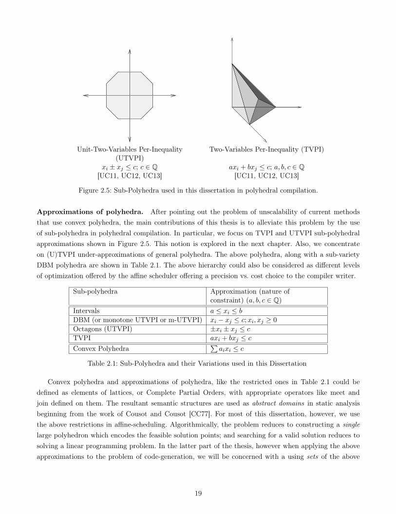
www.dedoimedo.com all rights reserved
Unit-Two-Variables Per-Inequality(UTVPI)
Two-Variables Per-Inequality (TVPI)
xi ± xj ≤ c; c ∈ Q axi + bxj ≤ c; a, b, c ∈ Q[UC11, UC12, UC13] [UC11, UC12, UC13]
Figure 2.5: Sub-Polyhedra used in this dissertation in polyhedral compilation.
Approximations of polyhedra. After pointing out the problem of unscalability of current methodsthat use convex polyhedra, the main contributions of this thesis is to alleviate this problem by the useof sub-polyhedra in polyhedral compilation. In particular, we focus on TVPI and UTVPI sub-polyhedralapproximations shown in Figure 2.5. This notion is explored in the next chapter. Also, we concentrateon (U)TVPI under-approximations of general polyhedra. The above polyhedra, along with a sub-varietyDBM polyhedra are shown in Table 2.1. The above hierarchy could also be considered as different levelsof optimization offered by the affine scheduler offering a precision vs. cost choice to the compiler writer.
Sub-polyhedra Approximation (nature ofconstraint) (a, b, c ∈ Q)
Intervals a ≤ xi ≤ bDBM (or monotone UTVPI or m-UTVPI) xi − xj ≤ c;xi, xj ≥ 0
Octagons (UTVPI) ±xi ± xj ≤ cTVPI axi + bxj ≤ cConvex Polyhedra
∑aixi ≤ c
Table 2.1: Sub-Polyhedra and their Variations used in this Dissertation
Convex polyhedra and approximations of polyhedra, like the restricted ones in Table 2.1 could bedefined as elements of lattices, or Complete Partial Orders, with appropriate operators like meet andjoin defined on them. The resultant semantic structures are used as abstract domains in static analysisbeginning from the work of Cousot and Cousot [CC77]. For most of this dissertation, however, we usethe above restrictions in affine-scheduling. Algorithmically, the problem reduces to constructing a singlelarge polyhedron which encodes the feasible solution points; and searching for a valid solution reduces tosolving a linear programming problem. In the latter part of the thesis, however when applying the aboveapproximations to the problem of code-generation, we will be concerned with a using sets of the above
19
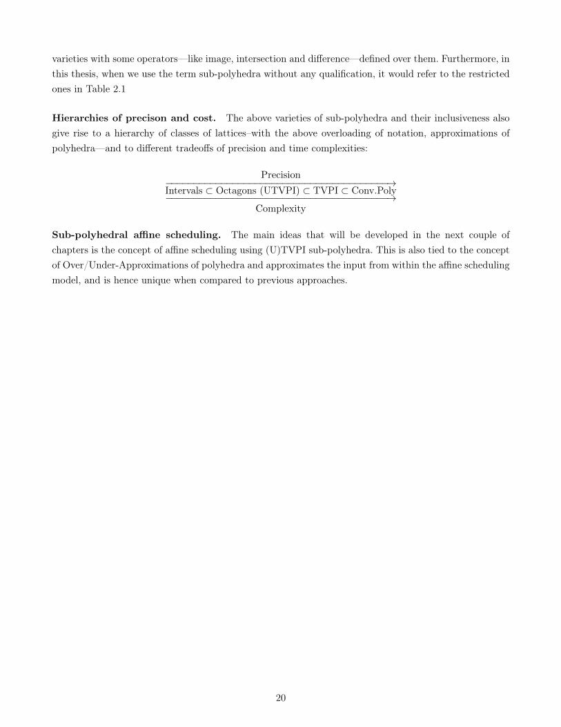
www.dedoimedo.com all rights reserved
varieties with some operators—like image, intersection and difference—defined over them. Furthermore, inthis thesis, when we use the term sub-polyhedra without any qualification, it would refer to the restrictedones in Table 2.1
Hierarchies of precison and cost. The above varieties of sub-polyhedra and their inclusiveness alsogive rise to a hierarchy of classes of lattices–with the above overloading of notation, approximations ofpolyhedra—and to different tradeoffs of precision and time complexities:
Precision−−−−−−−−−−−−−−−−−−−−−−−−−−−−−−−−−−−−−−−−→Intervals ⊂ Octagons (UTVPI) ⊂ TVPI ⊂ Conv.Poly−−−−−−−−−−−−−−−−−−−−−−−−−−−−−−−−−−−−−−−−→
Complexity
Sub-polyhedral affine scheduling. The main ideas that will be developed in the next couple ofchapters is the concept of affine scheduling using (U)TVPI sub-polyhedra. This is also tied to the conceptof Over/Under-Approximations of polyhedra and approximates the input from within the affine schedulingmodel, and is hence unique when compared to previous approaches.
20
Chapter 3
Sub-Polyhedra: TVPI and UTVPI
In this chapter, we briefly cover some basics of Two-Variables-Per-Inequality (TVPI) and (Unit-)Two-Variables-Per-Inequality (UTVPI) approximations of polyhedra.
−−−−−−−−−−−−−−−−−−−−−−−−−−→Interval ⊂ UTVPI ⊂ TVPI ⊂ Poly
Figure 3.1: A Hierarchy of Sub Polyhedral Classes
3.1 Introduction
In Section 3.2, we cover some complexities of (U)TVPI Sub-Polyhedra. In Section 3.3, we cover somebasics of Linear programming and Simplex complexity. This is followed by Section 3.4, where we studyhow (U)TVPI Sub-polyhedra fare when compared with general convex polyhedra in a complexity theoreticsense.
Prior to our work in loop parallelization, the static analysis field in recent times has seen a widespreadusage of sub-polyhedra. In Section 3.5, we do a brief summary of their use, and then differentiate on howtheir requirements are different from our proposed use of sub-polyhedra. A similar summary of the use ofsub-polyhedral abstractions by the loop parallelization community is done in the next chapter.
This will be followed with some conclusions and related work in Section 3.7.
Notation. For a polyhedron described in constraint form, let m be the number of inequalities, n be thenumber of variables and B the upper bound on the absolute value of the coefficients describing the system.
21
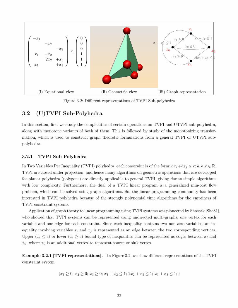
www.dedoimedo.com all rights reserved
−x1−x2
−x3x1 +x2
2x2 +x3x1 +x3
≤
000111
x1
x2x0
x3
x1 + x2 ≤ 1
x3 ≥ 0
x1 ≥ 0
x2 ≥ 0
2x2 + x3 ≤ 1
x1 + x3 ≤ 1
(i) Equational view (ii) Geometric view (iii) Graph representation
Figure 3.2: Different representations of TVPI Sub-polyhedra
3.2 (U)TVPI Sub-Polyhedra
In this section, first we study the complexities of certain operations on TVPI and UTVPI sub-polyhedra,along with monotone variants of both of them. This is followed by study of the monotonizing transfor-mation, which is used to construct graph theoretic formulations from a general TVPI or UTVPI sub-polyhedra.
3.2.1 TVPI Sub-Polyhedra
In Two Variables Per Inequality (TVPI) polyhedra, each constraint is of the form: axi+bxj ≤ c; a, b, c ∈ R.TVPI are closed under projection, and hence many algorithms on geometric operations that are developedfor planar polyhedra (polygons) are directly applicable to general TVPI, giving rise to simple algorithmswith low complexity. Furthermore, the dual of a TVPI linear program is a generalized min-cost flowproblem, which can be solved using graph algorithms. So, the linear programming community has beeninterested in TVPI polyhedra because of the strongly polynomial time algorithms for the emptiness ofTVPI constraint systems.
Application of graph theory to linear programming using TVPI systems was pioneered by Shostak [Sho81],who showed that TVPI systems can be represented using undirected multi-graphs: one vertex for eachvariable and one edge for each constraint. Since each inequality contains two non-zero variables, an in-equality involving variables xi and xj is represented as an edge between the two corresponding vertices.Upper (xi ≤ c) or lower (xi ≥ c) bound type of inequalities can be represented as edges between xi andx0, where x0 is an additional vertex to represent source or sink vertex.
Example 3.2.1 [TVPI representations]. In Figure 3.2, we show different representations of the TVPIconstraint system
{x1 ≥ 0; x2 ≥ 0; x3 ≥ 0; x1 + x2 ≤ 1; 2x2 + x3 ≤ 1; x1 + x3 ≤ 1; }
22
www.dedoimedo.com all rights reserved
the equational view, the geometric view3 and the graph representation.Aspvall and Shiloach [AS80] showed the polynomiality of the feasibility problem of TVPI-LP formula-
tions by introducing a unique strongly polynomial time procedure (“rumor in Grapevine algorithm”) thatcan be used to decide the range of a particular variable xi with respect to a given constant ξ. This latterprocedure is a Bellman-Ford style propagation of values assigned to variables through inequalities in thesystem, and is the heart of all subsequent algorithms in the TVPI literature.
Briefly, in the above algorithm, Aspvall and Shiloach make the assignment xi = ξ. As the inequalitiesin which xi participates are encoded as edges in the graph, the assignments to the neighbours of xi in thegraphical representation changes and they find corresponding assignments. These assignments percolatein the graph exchanging mutual assignments between neighbours, until a contradiction is found or allinequalities are satisfied. Shostak had earlier suggested an algorithm which enumerates simple cycles inthe graph for the same purpose and hence takes exponential time for such percolation, but Aspvall andShiloach show that the percolation can proceed in a controlled manner just similar to Bellman-Fordalgorithm. The complexity of Aspvall and Shiloach [AS80]’s percolation algorithm is the following:
Lemma 3.2.2 [Deciding a range of a variable in a TVPI system]. In a non-trivial TVPI system,given a variable xi and a numerical value (constant) ξ, it can be decided in O(mn) worst-case time whether(i) ξ < xmin
i , (i) xmini ≤ ξ ≤ xmax
i , or (iii) xmaxi < ξ.
The above complexity measure should be contrasted with the corresponding complexity measure ofthe analogous problem on general polyhedra which involves formulating an LP optimization problem andhence is as hard as LP-optimization.
The following result by Wayne [Way99] is the best to date for the TVPI optimization problem:
Lemma 3.2.3 [LP optimization on TVPI]. Linear programming optimization on TVPI systems canbe solved in O(m3n2 logm logB) worst-case time.
It well known that for general polyhedra, the optimization and the feasibility problems have thesame weakly-polynomial time hardness. But it is interesting to note that up to now, they have differentcomplexities on TVPI systems. The feasibility problem on TVPI systems has lower complexity that theabove weakly polynomial time result by Wayne [Way99] on the optimization problem. If we denote A as thecoefficient matrix of the system, B = bitsize(A), the upper-bound on the absolute value of the coefficientsdescribing the system, and the dependence of the above measure on B makes it weakly polynomial time.
The above complexity measure by Wayne is a general result with no restrictions on the type of objectivefunction. There exist improved complexity results for TVPI systems when the objective-function is of arestricted variety; for example, systems with bounded number of non-zero elements in the objective functionby Hochbaum and Naor [HN94] and systems with all coefficients of the objective function having the samesign by Hochbaum et al. [HMNT93].
The first strongly polynomial time algorithm for TVPI feasibility was given by Megiddo [Meg83].Network flow based (“combinatorial”) strongly polynomial time algorithms for the feasibility problem
3The 3-dimensional polyhedra in this chapter are drawn using polymake [GJ00] software.
23
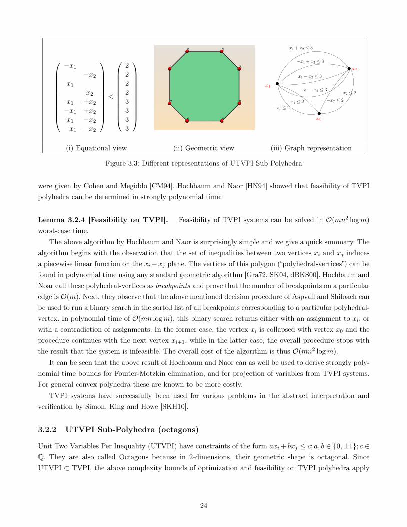
www.dedoimedo.com all rights reserved
−x1−x2
x1x2
x1 +x2−x1 +x2x1 −x2−x1 −x2
≤
22223333
x2
−x1 ≤ 2
x1 ≤ 2
−x1 − x2 ≤ 3
x1 − x2 ≤ 3
−x1 + x2 ≤ 3
x1 + x2 ≤ 3
x2 ≤ 2
−x2 ≤ 2
x1
x0
(i) Equational view (ii) Geometric view (iii) Graph representation
Figure 3.3: Different representations of UTVPI Sub-Polyhedra
were given by Cohen and Megiddo [CM94]. Hochbaum and Naor [HN94] showed that feasibility of TVPIpolyhedra can be determined in strongly polynomial time:
Lemma 3.2.4 [Feasibility on TVPI]. Feasibility of TVPI systems can be solved in O(mn2 logm)
worst-case time.The above algorithm by Hochbaum and Naor is surprisingly simple and we give a quick summary. The
algorithm begins with the observation that the set of inequalities between two vertices xi and xj inducesa piecewise linear function on the xi−xj plane. The vertices of this polygon (“polyhedral-vertices”) can befound in polynomial time using any standard geometric algorithm [Gra72, SK04, dBKS00]. Hochbaum andNoar call these polyhedral-vertices as breakpoints and prove that the number of breakpoints on a particularedge is O(m). Next, they observe that the above mentioned decision procedure of Aspvall and Shiloach canbe used to run a binary search in the sorted list of all breakpoints corresponding to a particular polyhedral-vertex. In polynomial time of O(mn logm), this binary search returns either with an assignment to xi, orwith a contradiction of assignments. In the former case, the vertex xi is collapsed with vertex x0 and theprocedure continues with the next vertex xi+1, while in the latter case, the overall procedure stops withthe result that the system is infeasible. The overall cost of the algorithm is thus O(mn2 logm).
It can be seen that the above result of Hochbaum and Naor can as well be used to derive strongly poly-nomial time bounds for Fourier-Motzkin elimination, and for projection of variables from TVPI systems.For general convex polyhedra these are known to be more costly.
TVPI systems have successfully been used for various problems in the abstract interpretation andverification by Simon, King and Howe [SKH10].
3.2.2 UTVPI Sub-Polyhedra (octagons)
Unit Two Variables Per Inequality (UTVPI) have constraints of the form axi + bxj ≤ c; a, b ∈ {0,±1}; c ∈Q. They are also called Octagons because in 2-dimensions, their geometric shape is octagonal. SinceUTVPI ⊂ TVPI, the above complexity bounds of optimization and feasibility on TVPI polyhedra apply
24

www.dedoimedo.com all rights reserved
to UTVPI polyhedra as well. But, as the dual of the LP formulation of shortest-paths problem has justdifference constraints [Pra77] with the form xi − xj ≤ c, general UTVPI systems can be solved with samequadratic complexity as Bellman-Ford [AMO93, CSRL01], giving the following lemma:
Lemma 3.2.5 [Feasibility on UTVPI]. Feasibility of UTVPI systems can be solved in O(mn) worst-case time and in O(m+ n) space.
The above decision algorithm can also trivially return a feasibility certificate of the UTVPI polyhedron.
Example 3.2.6 [UTVPI representations]. In Figure 3.3, we show different representations of theUTVPI system
{−2 ≤ x1, x2 ≤ 2; x1 + x2 ≤ 3; +x1 − x2 ≤ 3; −x1 + x2 ≤ 3; −x1 − x2 ≤ 3; }
the equational view, the geometric view and the graph representations.UTVPI polyhedra have successfully been used for various problems in abstract interpretation and
program verification [Min06, BHZ09, Min04]. Also, they have well supported libraries like Apron [JM09],and in the Parma Polyhedra Library (PPL) [BHZ08, PPL]. These are used with success in static-analysistools like the Astrée analyzer [BCC+03, CCF+09].
Monotone-UTVPI Sub-polyhedra (Diffference constraints). It can be noticed that differenceconstraints of the form xi − xj ≤ c are a specialization of UTVPI polyhedra. As mentioned, the polyno-miality of solving difference constraints using shortest paths algorithms of graph theory originates fromthe theory of Pratt [Pra77]. They have been called monotone constraints [Hoc04, HN94, CM94] becauseof the monotone nature of the sign of the coefficients, and constraint graph [CSRL01, AMO93] becausethey can be represented using weighed directed multi-graphs: one vertex per variable and one edge perconstraint with the directed edge for constraint xi − xj ≤ c being xj c−→ xi.
Their use as abstract domains is mainly by Bagnara et al. [Bag97], Miné et al. [Min01a] and Shahamet al. [SKS00] who call them Difference Bound Matrices (DBM), potential constraints, and zones.
It can noted that monotone-UTVPI constraints are quite similar to UTVPI constraints in that bothof these allow only two non-zero variables with only unit coefficients. But, UTVPIs can even encodeconstraints of the form xi + xj ≤ c and −xi − xj ≤ c as well, and even the upper-bound and lower-boundconstraints −xi ≤ c and xi ≤ c. Also, it can be noted that for both TVPI as well as UTVPI constraints,the graphs in their graphical representation are undirected and the constraints are just annotations onthe (undirected) edges. Both these restrictions can be removed for either of (U)TVPI systems using amonotonizing transformation.
3.2.3 Monotonizing transformation, Integer polyhedra and Feasibility
The monotonizing transformation takes in a normal (non-monotone) (U)TVPI constraint system, andcreates an equivalent monotone (U)TVPI constraint system having 2n variables: each variable xi in the
25

www.dedoimedo.com all rights reserved
original system would be represented by two variables x+i and x−i in the new system with xi = x+i = −x−i .The constraints in the new system are defined as in in Table 3.1.
TVPI monotonizing transformation. Given a TVPI system, the monotonizing transformation con-verts TVPI constraints to m-TVPI constraints (as in Table 3.1)
TVPIconstraint(a, b ∈ Q+)
Monotone representation
(++ case) axi + bxj ≤ c i 6= j ax+i − bx−j ≤ c ∧ −ax−i +bx+j ≤ c(−− case) −axi − bxj ≤ c i 6= j −ax+i +bx−j ≤ c ∧ ax−i − bx+j ≤ c
(+− case) axi − bxj ≤ c i 6= j ax+i − bx+j ≤ c ∧ −ax−i +bx−j ≤ c(−+ case) −axi + bxj ≤ c i 6= j −ax+i +bx+j ≤ c ∧ ax−i − bx−j ≤ c
(+0 case) axi ≤ c ax+i − ax−i ≤2c
(−0 case) −axi ≤ c −ax+i + ax−i ≤2c
Table 3.1: Monotonizing for converting TVPIs into monotone-TVPIs
It can be seen that in the new monotonized system is TVPI as well, with each constraint havingexactly one positive coefficient element and exactly one negative coefficient element with no other typesof constraints (like, for example between two elements with positive coefficients). Hence, the system canbe encoded as a directed graph with the direction of edges from the negative coefficient vertices to thepositive coefficient vertices. We call the monotone versions of TVPI as MTVPI constraints. The monotoneversions of UTVPI of course are MUTVPI or DBM constraints. The monotonizing transformation hasbeen invented and used many times, mostly in transforming the UTVPIs to MUTVPIs, but the above isin its most general form, where it is used to transform TVPI to MTVPI constraints.
Hidden behind the above monotonizing transformation is a rounding scheme of rationals into integers.This is because, integral general (non-monotone) TVPI and UTVPI systems are computationally morecomplex than their corresponding monotonized variations; these integral systems have NP-Complete re-ductions. As an example for the same, the constraints in the formulation of vertex cover problem (or itscomplement, the maximum independent set) have just two non-zero elements per row. Here is the ILPformulation of the same.
Vertex cover ILP formulation. Let G = (V,E) denote an undirected graph. Each vertex i ∈ V islabelled by a cost c(i) ≥ 0. The vertex cover problem is to find a cover, namely a collection of weightsxi ∈ Z for the vertices, so that the weighed sum
∑i∈V c(i)xi is minimized,
subject to
e = (i, j) ∈ E : xi + xj ≥ 1
1 ≤ i ≤ N ∈ V : xi ∈ {0, 1}
26
www.dedoimedo.com all rights reserved
The vertex cover problem is strongly NP-Complete, being one of Karp’s 21 classic problems [GJ79,prob. GT1, p. 190]. It can be seen that the constraints of the vertex cover problem are UTVPI constraintswith only the additional restriction that xi ∈ Z. But, it can be noticed that the constraints are non-monotone UTVPI. Enforcing them to be monotone and making a rational relaxation for each xi, namelyby xi ∈ Q; 0 ≤ xi ≤ 1 and solving the resultant MUTVPI constraints by graph theory methods would bean approximation algorithm [GLS93, GJ79] of the original NP-Complete algorithm.
When the original system is UTVPI, the above monotonizing transformation converts it into a To-tally Unimodular system, while the original may not be. Any MUTVPI (or DBM) system is Totally-Unimodular [Sch86, Chapter 19]. This is another illustration that solving MUTVPI system is computa-tionally simpler than solving general UTVPI systems.
3.3 Linear Programming on Convex Polyhedra
Linear Programming is one of the most powerful tools in the algorithmician’s toolkit and its history datesback to 1963 with Dantzig’s classic work [Dan63], coinciding with that of algorithms, and algorithmicanalysis itself. In 1979, Khachiyan (Hačijan) [Hač79] proved that Linear Programming can be solved inpolynomial time using ellipsoid method. This was followed by Karmarkar [Kar84], who introduced interiorpoint methods for the same. Though both the above algorithms have weakly polynomial time complexity,the former has only been a theoretical interest, while the latter have proved to have much practicalvalue beyond linear programming. They have been applied with much success to non-linear programmingproblems like quadratic programming, convex programming and semi-definite programming [BV04].
From Megiddo’s result [Meg84], it is known that when the dimension is fixed, the complexity of LP isstrongly polynomial, but no specific algorithm is known for the general case, i.e., when the dimension isalso considered a variable. Whether there exists a strongly polynomial time algorithm for simplex is stillan open question and it has been named in Smale’s 18 unsolved problems [Sma98] listed in 20004.
In spite of all the above, the most widely used algorithm for linear programming is the simplex algorithmitself, whose basic structure has not changed much since its original discovery by Dantzig [Dan63]. It hasbeen extremely successful and academia, research as well as industry would consider that a problem issolved when it is reduced to a LP which uses simplex algorithm. There are three views which are equivalentabout simplex algorithm:
• [Algorithmic] Simplex algorithm traverses the polytope5 from a vertex to its adjacent vertex.
• [Complexity] For any fixed pivoting rule, there exists a particular Klee-Minty cube, for which thesimplex algorithm traverses a hamiltonian path in the graph of the cube.
• [Combinatorial] The maximum path length of a traversal of simplex algorithm is upper-bounded bythe diameter of the graph of the polytope.
4in the spirit of Hilber’t 23 problems posed at the beginning of previous century5Though a polytope, a bounded polyhedron, is geometrically different from a polyhedron, algorithmically and combinato-
rially restricting the discussion to just polytopes does not pose any limitation; equivalence can be obtained by transformationslike homogenization and de-homogenization [Zie06]. Even tools like polymake [GJ00] support these transformations.
27
www.dedoimedo.com all rights reserved
3.3.1 Algorithmic and complexity theoretic view
The algorithmic view is well understood by basic linear programming. It is well known that simplexalgorithm achieves an optimal value at a vertex. To exploit this, Dantzig’s simplex algorithm, picks aparticular vertex in its first phase, and in the subsequent phases follows vertices adjacent to each otherin an iterative fashion, until further improvement in the cost function is not possible. This algorithmiccharacterization gave rise to many kinds of pivoting rules, ways in which the next adjacent vertex canbe picked. The bland’s rule, a trick to avoid degeneracy (or cycling), is used generally universally and isknown to work extremely well in practice [Bix02]. Bland’s rule, along with dual simplex strategy is usedas the engine of Feautrier’s famed PIP [Fea88] as well.
The Simplex algorithm’s success is a classic case of a local search strategy working extremely well on theaverage case. Spielman and Teng [ST04] even proposed smoothened analysis, a new method of algorithmicaverage case analysis, where the hard instances of the input are perturbed using some noise—gaussianwith zero mean and variance—so that an easy instance is obtained which runs in guaranteed polynomialtime with high probability. This method of Spielman and Teng is as much about average case analysis ofsimplex, as it is about perturbation analysis of algorithms.
Observation 3.3.1 [Experimental complexity of (LP using) simplex algorithm]. Let Z(m,n)
be the complexity of LP using the Simplex algorithm with m constraints and n variables. Determiningtypical value of Z is not an easy task, as it depends on many details of the algorithm, like the pivotingrule, the method to exploit sparsity, and even many implementation details, like ratio of m and n, thetype of arithmetic used: fixed vs. arbitrary-precision, integers vs. rationals and so on. In this dissertationhowever, and only for some empirical comparisons, we use the following folklore result which does notcount the bit-size complexity: On a typical input, Z(m,n) = O((m+ n)mn) on average.
Even though we have added the above caveats, we should note that the above estimate is practicallyvery accurate for the LP programs we observe. In the above empirical estimate, which is obviously notstrongly polynomial time (in which we are not counting the bits), we assume that the gaussian eliminationsteps of the simplex are very fast, exploiting sparsity, and assuming a linear number O(m+n) of pivotingsteps. Similar conclusions have been made in the literature as well. For example, Todd [Tod02] says: “...remarkable fact: the primal simplex method typically requires at most 2m to 3m pivots to attain optimality”.
Complexity theoretic view. The complexity theoretic or worst-case view is best explained by theKlee-Minty traversal, where all the vertices are traversed by the simplex algorithm as in Figure 3.4 onthe facing page.(i). The exponentiality of the simplex method was proved by Klee and Minty [KM72]. Forevery fixed pivot rule, there exists a version of Klee-Minty cube. Also, the exponentiality of Klee-Mintyillustrates that the initial local search choice spoils the whole search mechanism. In either of the cases inFigures 3.4 on the next page.(i), the simplex algorithm could have reached the optimal value in one stepinstead of traversing a path that touches all the vertices before returning to the final optimum point. Thepath of Simplex on the Klee-Minty cubes could be considered as a hamiltonian path on the graph of thepolytope [Zie06, Chapter 3], whose vertices are the vertices (0-dimensional faces) of the polytopes, and
28

www.dedoimedo.com all rights reserved
d=3
(i) Simplex traversal inworst-case
(ii) Graph and diameter of ahypercube
Figure 3.4: Simplex traversal, Klee-Minty style traversal, and Graph and diameter of a polytope
whose edges are the edges (1-dimensional faces) of the polytope (a 3d cube) as shown in Figure 3.4.(ii).
3.3.2 Combinatorial view
The combinatorial view has to do with recent advances in geometry with the diameter of the graph andthe Hirsch conjecture [Zie06] of 1957:
Hirsch conjecture. Let m > d ≥ 2 and let P be a d-dimensional polytope with m-facets (inequalities),and let G(P ) be its graph. Then diam(G(P )) ≤ m− d.
Having been unresolved for more than half a century, the Hirsch conjecture has been proved to be in-correct by Santos [San10] in 2010, who gave a counterexample for it. Santos’s proof consists of constructinga 43-dimensional polytope (a prismatoid) with 86 facets having a diameter greater than 43. After Santosconstruction, smaller dimensional constructions have been given.
Remark about Hirsch conjecture and observation. 3.3.1 In the estimate in Observation 3.3.1,we are just assuming that for normal cases in polyhedral compilation, we are observing linear numberof pivots, namely O(m + n). This could mean m + n pivots, 2(m + n) pivots, 2m + 3m pivots etc., asobserved by Todd [Tod02]. The recent Hirsch conjecture disproval on the other hand is about the problemcomplexity, not algorithmic complexity, and is about absence of any linear time path for any polytope;this does not mean a O(m + n) number of pivots, but exactly m − d. Hence, it being disproved by theabove mentioned work of Santos does not have practical implications, and our estimate is independent ofthe recent disproval of Hirsch conjecture.
A variation of Hirsch conjecture may be true for polyhedra: namely there may be two constants aand b such that diameter is always am+ bd. This new conjecture is still open and is called Linear HirschConjecture.
Linear Hirsch conjecture. Is there a linear function f(m, d) such that for any polytope P of dimensiond and with m facets, diam(G(P )) ≤ f(m, d)?
29

www.dedoimedo.com all rights reserved
Problem ConvexPolyhedra
TVPI m-TVPI UTVPI m-UTVPI(DBM)
LPFEAS WPT O(mn2 logm) O(mn)LPOPT WPT O(m3n2 logm logB) X
ILPFEAS SNPC SNPC WNPC SNPC XILPOPT SNPC SNPC WNPC SNPC X
Fourier-Motzkin
O(m2n) O(mn2 logm) O(mn2 logm)
GEN (V ↔ H) EXP(n),EXP(d)
EXP(n),EXP(d) EXP(n), EXP(d)
Table 3.2: Convex Polyhedra, (U)TVPI Sub-Polyhedra and monotone (U)TVPI Sub-Polyhedra: Com-parison of (worst-case) complexities. The problem complexities are denoted in red, while the worst-casecomplexities of the best known algorithms are denoted in blue. Also, X = O((m log n)(m+ n log n)).
The above linear Hirsch conjecture, as well as similar polynomial variations of it, are still open at thetime of this writing. If any of them are proved to be correct, then the implications of solving LP throughSimplex could be huge [KS10] mainly because of the bridge they would make between the gap betweenthe intuitive understanding of the algorithm and its theoretical complexity.
3.4 Complexities of Convex Polyhedra and Sub-polyhedra
In Table 3.2, we summarize the relevant complexities6 of general convex polyhedra with TVPI and UTVPISub-Polyhedra along with their monotone versions. Each problem instance is defined to be in n variables,m inequalities and d dimensions. For complexities that are not exactly known, we will be using theircorresponding complexity class. More specifially, WPT stands for Weakly Polynomial Time, and SNPCand WNPC stand for Strongly NP-Complete and Weakly NP-Complete respectively7.
Linear Programming (rational) feasibility (LPFEAS). The LPFEAS problem has weakly polyno-mial time complexity for convex polyhedra. On TVPI polyhedra, it has strongly polynomial time complex-ity because of results of Hochbaum-Naor [HN94] and Cohen-Megiddo [CM94]. Since the problem is definedover rational polyhedra on which the monotonization transformation does not change the precision, thenon-monotone variants of the problem on both TVPI and UTVPI polyhedra have the same complexitiesas their monotone variants. The complexity of feasibility of UTVPI polyhedra and m-UTVPI polyhedrais the complexity of Bellman-Ford algorithm [Bel58, FF62].
Linear Programming (rational) Optimization (LPOPT). The LPOPT problem on convex poly-hedra is weakly polynomial time. On TVPI polyhedra, the complexity is O(m3n2 logm logB) due to theresult of Wayne [Way99]. Though better than convex polyhedra, it is still weakly polynomial time due
6In this table, we take a little liberty of mixing problem complexities with algorithm complexities.7We thank Dorit Hochbaum for suggesting corrections to this table.
30
www.dedoimedo.com all rights reserved
to presence of B in the complexity formula. For UTVPI polyhedra, as the constraint matrix has only{0,±1} elements, the problem has strongly polynomial time complexity. Using the duality result of linearprogramming, the flow problems–of which min-cost-flow and Bellman-Ford problems could be consideredas special cases, for TVPI and UTVPI polyhedra respectively–can be shown to have the same complexitiesas the LPOPT problem.
Integer Linear Programming Feasibility/Optimization (ILPFEAS/ILPOPT). The ILPFEASproblem is well known to be strongly NP-Complete [GJ79, prob. MP1, p.245] for convex polyhedra. OnTVPI polyhedra, the problem has been proved to be strongly NP-Complete by Lagarias [Lag85]. Forgeneral UTVPI polyhedra as well, the same complexity holds as the vertex cover problem can be reducedto it. But, the corresponding problem over monotone TVPI systems is weakly NP-Complete as provedby Hochbaum-Naor [HN94] with complexity O(mnB2 log(Bn2/m)). For monotone UTVPI polyhedra, thecorresponding complexity is O(mn log(n2/m)) which is clearly strongly polynomial time. All the entriesin the ILPOPT row have the same complexities as the corresponding complexities as ILPFEAS. (Thoughstrictly speaking, only decision problems are tackled by NP-Completeness.)
Fourier-Motzkin. The problem of Fourier-Motzkin is well known to be doubly exponential in thenumber of variables with the number of inequalities rising to an exhorbitant bm2 c2
n . Hochbaum-Naor’sresult on the other hand shows the polynomiality for TVPI polyhedra. The same result applies to forUTVPI polyhedra as well.
Generator representation (GEN (V ↔ H)). Even for Interval polyhedra, the problem of convertingfrom constraint to generator representation is exponential as illustrated by the n-dimensional hypercube.Hence this problem is exponential for any of the polyhedra and sub-polyhedral classes (or lattices) con-sidered.
3.5 Polyhedral Approximations in Static Analysis
The static analysis community has been considering the tradeoffs between different Sub-Polyhedra as ameans of trading expressiveness for computational complexity in solving abstract interpretation prob-lems [CC77]. The pioneering work of Cousot and Cousot [CC76] introduced Interval (Interval) abstractdomain, and was followed by the introduction of Polyhedron (Poly) abstract domain by Cousot and Halb-wachs [CH78]. In recent times, this was followed by the breakthrough work by Miné [Min01a] on Octagonabstract domain (Octagons) in 2001. This work led to the use of many Sub-Polyhedra which have beenfound to be both expressive enough as well as cost effective for many static analysis and other run-timeprogram verification problems like value range analysis, bounds checking of indices of array variables, bufferoverflows, validation of array accesses etc. It is interesting that almost the entire range of Sub-Polyhedralabstract domains being used in recent times fit within the range defined by the works of Cousot, Cousotand Halbwachs in the late 70s: interval abstract domain by Cousot and Cousot [CC76], and polyhedronabstract domain by Cousot and Halbwachs [CH78].
31
www.dedoimedo.com all rights reserved
In formulating these applications, the static analysis community uses descriptions of programs calledabstract domains. An abstract domain is presented as a lattice 〈D,v,t,u〉, with v being an orderingpredicate, and u and t being the associated meet and join operators respectively. Many of the staticanalysis problems can be formulated as general polyhedral operations in the Poly abstract domain, inwhich D are convex sets that can be described by finite number of general linear inequalities. But thestatic analysis community has found Poly to be too expensive for the applications of interest, for severalreasons.
Firstly, the need for join (t) operators on polyhedra. The most precise join operation calculates the clo-sure of the convex hull of the two input polyhedra, that is, a set of inequalities that represent the smallestspace that includes the two input polyhedra. One straightforward way to do the above is to use the gener-ator representation of the two polyhedra and compute the convex hull. This method needs the generatorrepresentation of both of them, and a conversion from constraint representation to generator representationand back. Hence it can take exponential time as convex-hull of even two d-dimensional hypercubes requiresjust 2d inequalities for each hypercube, while needing 2d vertices. In spite of many practical techniques toreduce the complexity, the asymptotic cost cannot be reduced by a large amount [HMG06].
Secondly, it is the recursive nature of (flow) equations which are solved in an iterative way until a fix-point is reached. In solving these equations, the meet (u) operator usually adds a few additional inequalitiesto an existing system and then the system is used for other operations like entailment checks (checkingif P1 ⊆ P2 holds), or subjected again to join or even the projection operations. These requirements leadto the need for a so called closed system, in which all information between any pairs of variables can beinferred by using the set of constraints that involve only those pairs of variables. An example illustratingfor closure operation on a TVPI system is annotating the system {ax+ by ≤ c; dx+ ez ≤ f ; } by theadditional implied constraint aez − bdy ≤ af − cd if a > 0 ∧ d < 0, so that the relationship betweenvariables y and z can be discovered in constant time. Geometrically, closure can also be considered as theprocess of calculating all possible projections. Needless to say, closure is very costly for Poly.
Finally, another reason is the scale of problems that are being dealt with. For the more demandingapplications coming from run-time verification problems, the more powerful Poly are simply unaffordable.Miné [Min06, page 4] says “... polyhedron domain has a memory and time cost unbounded in theory andexponential in practice”, while Laviron and Logozzo [LL09, page 2] say “... Poly easily propagates theconstraints. However, ... the price to pay for using Poly is too high: the analysis not scale beyond dozensof variables, ... while mostly one wants to solve hundreds of constraints and variables.”. These results arefurther substantiated in the earlier study by Halbwachs et al. [HMG06]. It should also be noted that theabstract interpretation problems also have to deal with memory scalability problems because of large sizeof input instances that they aim to solve. The combined effects of the high cost of time as well as spacecomplexities of Poly cause the above mentioned scalability issues.
Hence, Sub-Polyhedral abstract domains started being used, by either restricting the shape of the poly-hedron (the weakly relational domain approach) or by a priori limiting the number of linear-inequalitiesthat can be solved (the bounded domains approach). The most obvious in the first category are (mul-tidimensional) intervals, or “boxes”, which have been used by Cousot and Cousot [CC76]. Beyond these
32
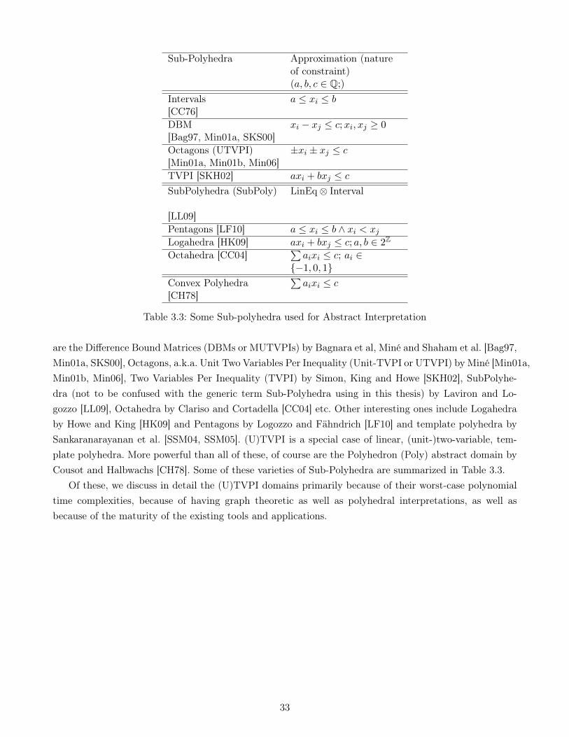
www.dedoimedo.com all rights reserved
Sub-Polyhedra Approximation (natureof constraint)(a, b, c ∈ Q;)
Intervals[CC76]
a ≤ xi ≤ b
DBM[Bag97, Min01a, SKS00]
xi − xj ≤ c;xi, xj ≥ 0
Octagons (UTVPI)[Min01a, Min01b, Min06]
±xi ± xj ≤ c
TVPI [SKH02] axi + bxj ≤ cSubPolyhedra (SubPoly)
[LL09]
LinEq⊗ Interval
Pentagons [LF10] a ≤ xi ≤ b ∧ xi < xjLogahedra [HK09] axi + bxj ≤ c; a, b ∈ 2Z
Octahedra [CC04]∑aixi ≤ c; ai ∈
{−1, 0, 1}Convex Polyhedra[CH78]
∑aixi ≤ c
Table 3.3: Some Sub-polyhedra used for Abstract Interpretation
are the Difference Bound Matrices (DBMs or MUTVPIs) by Bagnara et al, Miné and Shaham et al. [Bag97,Min01a, SKS00], Octagons, a.k.a. Unit Two Variables Per Inequality (Unit-TVPI or UTVPI) by Miné [Min01a,Min01b, Min06], Two Variables Per Inequality (TVPI) by Simon, King and Howe [SKH02], SubPolyhe-dra (not to be confused with the generic term Sub-Polyhedra using in this thesis) by Laviron and Lo-gozzo [LL09], Octahedra by Clariso and Cortadella [CC04] etc. Other interesting ones include Logahedraby Howe and King [HK09] and Pentagons by Logozzo and Fähndrich [LF10] and template polyhedra bySankaranarayanan et al. [SSM04, SSM05]. (U)TVPI is a special case of linear, (unit-)two-variable, tem-plate polyhedra. More powerful than all of these, of course are the Polyhedron (Poly) abstract domain byCousot and Halbwachs [CH78]. Some of these varieties of Sub-Polyhedra are summarized in Table 3.3.
Of these, we discuss in detail the (U)TVPI domains primarily because of their worst-case polynomialtime complexities, because of having graph theoretic as well as polyhedral interpretations, as well asbecause of the maturity of the existing tools and applications.
33

www.dedoimedo.com all rights reserved
3.6 A Summary of Related Work
In this section quickly (re-)summarize the related work. Though this chapter had summaries of variousworks at different places, it is intended that this kind of summarization of related work at a single placewould help in understanding the complexity context of sub-polyhedra, as well as place in focus our searchfor proper abstractions with the correct asymptotic complexities.
Algorithms for (U)TVPI Sub-Polyhedra. Sub-polyhedra, in particular (U)TVPI polyhedra hadbeen of interest to the theoretical and algorithmic community because of the search for strongly polynomialtime algorithms. UTVPI was pioneered by the work of Pratt [Pra77], while TVPI was by Megiddo [Meg83].The state of the art in feasibility testing for TVPI systems is strongly polynomial time algorithms byHochbaum and Naor [HN94], and Cohen and Megiddo [CM94] and for optimization of TVPI systems isweakly polynomial time algorithms by Wayne [Way99]. We are not aware of existing implementations ofthe above algorithms.
The strongly polynomial time algorithms for TVPI system for feasibility [HN94, CM94] should be con-trasted with the weakly polynomial time algorithm by Wayne [Way99]. This discrepancy is an example ofa complexity theoretic duality gap between the two problems. At the time of this writing, no strongly poly-nomial time algorithm is known for general optimization, namely objective function of arbitrary length, onTVPI polyhedra. Special cases, like maximization of a single variable and finding lexicographic maximumcan be solved using the strongly polynomial algorithms which solve feasibility.
The state of the art for feasibility and optimization of UTVPI systems is by the well understoodBellman-Ford algorithm, which involves constructing a nearly 2m × 2n size incidence matrix (constraintgraph) encoding the difference constraints of the monotonized system and testing it for presence ofnegative weight cycles using the shortest-path problem. The latter has been extensively studied, begin-ning from [Bel58, FF62] to most recently in [CGG+10]. Efficient, though closure based methods for thesame [Min06, BHZ09] are available in Apron [JM09] and PPL [BHZ08, PPL].
Monotonizing transformation. The monotonizing transformation can be done either on TVPI orUTVPI constraints to obtain a TU matrix. It has a rich history from the study of pre-Leontief matricesby Dantzig: a general convex system where each constraint has at most one positive element is called apre-Leontief system. The reduction transformation of UTVPI to MUTVPI for algorithmic purposes seemsto have been re-invented many times, though Hochbaum [Hoc04, HN94] attributes the formalization of itsapplication to Edelsbrunner et al. [ERW89]. In the many works of Hochbaum like [HMNT93, Hoc98, HN94],it has been used for approximation of NP-Complete problems like vertex-cover, minimum-SAT, schedulingwith precedence constraints, generalized 2SAT etc. Even the dual version of monotonizing the columns hasbeen studied by Hochbaum [Hoc04] so that it can work as approximation algorithm for the flow problemswhose duals are TVPI programs, like maximum-cut problem (an NP-Complete problem) and generalizedflow problem. The abstract interpretation community has also been using it beginning with the work ofMiné [Min06], though the attributions in some references [LM05, SS10] are incorrect.
Our presentation on monotonization closely follows Hochbaum’s [Hoc04] and Miné’s [Min06, Min04]
34
www.dedoimedo.com all rights reserved
presentations. Miné [Min06] uses the above transformation for transforming the UTVPIs to MUTVPIs(DBMs). With such transformation, he uses an adjacency matrix representation for the DBM could beused for storing the original UTVPI constraints. Though we have covered the monotonization in its mostgeneral form, namely for TVPI constraints, for implementational reasons however, we would be convertingonly UTVPI systems into MUTVPI systems. Also, for most of this dissertation, we deal with rationalpolyhedra and hence, the loss of precision by monotonization does not affect us. An exception to this isin Chapter 8 on page 101, where we extend the already developed rational approximation framework toobtain integer approximatons of NP-Complete problems. Even for many abstract interpretation purposeslike the use of Octagons by Miné, the conversion of UTVPI’s to DBMs is not a concern as they too aremostly concerned with the emptiness of the rational polyhedron.
Simplex complexity and Hirsch conjecture. In the complexity aspect, Sub-polyhedra fare betterthan general convex polyhedra for which efficient algorithms are usually based on the widely used Simplexalgorithm [Dan63]. Schrijver [Sch86] is a good reference for linear programming, while Ziegler [Zie06] isfor the geometric aspects. Santos [San10, Zie06] disproved the Hirsch conjecture in 2010. Our presentationon Hirsch conjecture follows Kim and Santos’s expository paper [KS10] and Kim’s thesis [Kim10].
Sub-polyhedra in static analysis. The complexities of operations on general convex polyhedra areknown [JMSY94, HMG06, Min06] to be considerably more time consuming than (U)TVPI polyhedra forabstract domain operations. Hence, Sub-polyhedra have been widely employed in abstract interpretationproblems by the static analysis community as a means of trading precision for scalability. An excellentpresentation of Sub-Polyhedra and its applications to abstract interpretation can be found in Miné’sthesis [Min04]. A comparison of the use of these, as well as more varieties of Sub-Polyhedra, along withtheir applicability to polyhedral compilation can be found in our work [UC11]. Of the many classes ofSub-Polyhedra, (U)TVPI polyhedra have extensively been used [Min06, BHZ09, SK10], with impressiveresults such as in Astrée [BCC+03, CCF+09]. Surprisingly enough, UTVPI polyhedra have first been usedby Balasundaram-Kennedy [BK89] for loop parallelization applications. We will summarize their approachin the next chapter.
3.7 Conclusions, Contributions and Perspectives
In this section, we review the conclusions and contributions of this chapter, as well as discuss someperspectives.
Conclusions. In this chapter, we study the complexities of algorithms on (U)TVPI Sub-polyhedra. Weshowed that they have excellent theoretical properties that can be put to use in polyhedral compilation,and in particular affine scheduling. We also study the use of polyhedral sub-classes (Sub-polyhedra) asabstract domains by the static analysis community. We discovered that the static analysis community hasbeen exploiting the richness of sub-polyhedra as a means of trading precision for execution time, and thesame theme could help in obviating the scalability problem in the polyhedral compilation as well.
35
www.dedoimedo.com all rights reserved
Contributions. Our contribution is in understanding which Sub-polyhedra, among the ones which havebeen of interest to theoreticians or to the static analysis community, are possibly the best suited to reducethe complexity of affine scheduling. Part of this chapter has been published in [UC11].
Perspectives. One initial goal of this work was to see if any existing Sub-polyhedral libraries likeOctagons by Apron [JM09] and PPL [PPL] or TVPI by TVPI-lib [SKH02] can easily be adapted to be usedin the affine scheduling framework like the one developed in GRAPHITE [TCE+10]. We discovered that thereliance of the existing static analysis libraries on closure, and generator representation would be limitationsfor scheduling purposes. Addition of simplex solver in these existing libraries would not have helped theutility purpose of the libraries themselves because these varieties of sub-polyhedra are particularly suitedfor graph theory based methods of solution, not a tableau based one like simplex. Also, use of such an existinglibrary would still need an approximation algorithm, one that transforms a general convex polyhedroninto the chosen kind of Sub-polyhedra. Such algorithms have been not studied previously. This subject isdeveloped in a later chapter (Chapter 6).
In the next chapter we will first study various methods in which approximations can be used inpolyhedral compilation. This will be followed by proposal of a new scheme that uses (U)TVPI under-approximations of the polyhedra, by which low complexity algorithms of (U)TVPI polyhedra can beexploited.
36
Chapter 4
Polyhedral Scheduling and Approximations
4.1 Introduction
In Chapter 2 we showed that the current scheduling methods which are based on general convex polyhedraare unscalable. In Chapter 3 we studied various varieties of sub-polyhedra, along with a special emphasison (U)TVPI sub-polyhedra. We learnt that because of the low complexity operations on these lattervarieties, they could be used in affine scheduling. In this chapter, we study and propose methods to reducethe scalability bottleneck using (U)TVPI sub-polyhedra.
Overview of this section. Firstly, in the current section, we describe a rough method in which affinescheduling are made scalable. Next, in Section 4.2 we briefly discuss some previous techniques which havesimilar motivation as ours. This is followed by Section 4.3 where we study some existing algorithms thatapproximate a general convex polyhedron by a (U)TVPI polyhedron.
The above is followed by Section 4.4 where two new scheduling heuristic approaches which use sub-polyhedra are introduced, with an example to illustrate their working in Section 4.5. This is followed inSection 4.6 by a re-summarization of related work. Finally in Section 4.7, we present some conclusions,contributions, and perspectives.
4.1.1 Approaches for making affine scheduling scalable
The excellent worst-case complexities of operations and algorithms on sub-polyhedra provide a motivationfor using them in polyhedral scheduling. Whichever be the flavor of sub-polyhedra—whether they areTVPI or UTVPI or some other—some choices have to be made about its use. Furthermore, there could begeneral convex polyhedra based approaches, that attempt to improve the scalability problem by employingproper heuristics. Here is one classification of such methods8.
Dependence approximation. One may assume that the dependence polyhedra satisfy some criterion.The input to the optimization or parallelization problem is chosen to belong to a pre-determined flavor of
8The level of detail in this chapter is at an expert level. Though a quick introduction has been provided in Chapter 2, agentler introduction is in Darte et al. [DRV00, Chapter 5] and Bastoul [Bas12, Chapter 2].
37
www.dedoimedo.com all rights reserved
sub-polyhedra. The dependence sets which do not satisfy those criterion must be Over-approximated by analgorithm or heuristic. Some schedules may be lost, but only correct transformations will be modeled. Thisnecessary approximation is in the same spirit as classical abstractions and algorithms presented in [YAI95,DRV00]. We briefly discuss these classical dependence approximations in Section 4.2.1.1, and then by asimilar approach by Balasundaram-Kennedy [BK89] which uses UTVPI sub-polyhedra in Section 4.2.1.2.
Constraint (Farkas polyhedra) approximation. Another design choice is to keep the dependencerelations as general polyhedra, but approximate the constraints on the affine transformation itself. Afterthe transformation to the dual space through the Farkas lemma, the constraint polyhedron–the (µ, λ)-polyhedron of Farkas multipliers–must be Under-Approximated (UA). Again, some legal affine transfor-mations may be lost. We will discuss constraint approximation with (U)TVPI sub-polyhedra in Section 4.4.
Simplex-based methods. Beyond the above sub-polyhedral methods are simplex-based heuristic meth-ods. The approach of Feautrier in his modular scheduling [Fea06] involves reducing the complexity bycalling the simplex algorithm on smaller systems or modules as well as making the simplex method awareof the dependence graph structure. We will study his approach in Section 4.2.3.1. In Section 4.2.3.2, wepropose a new heuristic by which the simplex algorithm itself could be tuned to have fixed number ofpivots so as to reduce its complexity.
Additional approximations. There are at least two more ways to use sub-polyhedra in polyhedralscheduling. These are domain approximation and objective function approximation. In most cases, iterationdomains defined by the loop bounds form multi-dimensional intervals, and most non-interval cases belongto the UTVPI flavor or triangular loops: As observed by Feautrier [Fea92a], “In nearly all practicalcases, each iteration domain is defined by two inequalities per loop”. Approximations are possible, butrequire specific handling in the code generator to generate precise iteration domain traversals; we believethe problem can be reduced to code generation for irregular, data-dependent control flow [BPCB10].Regarding the approximation of objective functions, the strongly polynomial time bounds for (U)TVPIpolyhedra discussed in Chapter 3 only holds for a specific class of feasibility and optimization problems:when the objective function has bounded number of elements, or when they have the same sign, or whenit is a lexicographic maximum. When the objective function is arbitrary, linear programming seems to berequired. This is discussed in detail in the literature [HN94, CM94, Way99]. We believe solutions can befound to enable both kinds of approximations, but leave these as open problems.
4.1.2 Conditions for approximation
A general polyhedron has to be converted into a Sub-polyhedra for it use the algorithms or librariesthat specialize in it. An approximation can be an over or an under-approximation. In both cases, theapproximation algorithm must consider some issues:
• Legality: The approximated polyhedron should not yield illegal optimizations. Since the main em-phasis is on correctness of the transformation, the approximation should satisfy legality conditions.
38

www.dedoimedo.com all rights reserved
Examples for legal transformations are over-approximations in the dependence polyhedron space andunder-approximations in the Farkas-polyhedron space.
• Cost: Low complexity running time: The conversion process should be asymptotically small (polynomial-time) as well as appreciably simpler. Further, it is preferable if its complexity is strongly polynomial.
• Tightness: The approximated polyhedron should be as close to the original polyhedron as possible.In case of rational approximation, the volume of the approximated sub-polyhedron should be asclose to the original one as possible. In case of integer approximation, it should leave-out/add as fewnumber of integer points as possible.
• Expressiveness: The approximation should give non-trivial results—feasible, non-degenerate polyhedra—for a sizable number of interesting inputs. Also, if the approximation algorithm does not take intoaccount the objective functions, the feasible points in the result may not yield very interesting affinetransformations in terms of the optimization problem they are attempting to address. Both feasibil-ity and objective function affect the expressiveness of the overall approach. This expressiveness canbe measured in terms of the quality of the overall optimization on approximate sub-polyhedra.
There are some more constraints that the algorithm must satisfy. We point them in Section 4.2.1.1 and 4.4.
4.2 Some Existing Approaches for Scalable Loop Transformations
In this section, we cover some existing approaches which can be adapted for scalability purposes, andones which had already attempted to do so. First we quickly summarize the classic dependence over-approximations [YAI95] in the parallelization literature. Then, we summarize another early approachproposed by Balasundaram-Kennedy [BK89] which uses UTVPI polyhedra for task level parallelism pur-poses. This is followed by studying Creusillet’s approach [Cre96] who proposed scalable approaches forarray region analysis using both under- and over-approximations. Next, we summarize Feautrier’s modu-lar scheduling approach [Fea06] which is the first in the affine scheduling literature to declare the simplexalgorithm itself as the main culprit of scalability. We also introduce a new method that involves tuning thesimplex algorithm to run with fixed number of pivots, and follow with some miscellaneous alternatives,like the vertex method.
4.2.1 Dependence Over-Approximations
4.2.1.1 Classic dependence over-approximations
Over-approximations of dependence polyhedra, including sub-polyhedra and beyond-polyhedral abstrac-tions, is a fairly well-known technique and have already been used in parallelization. This kind of depen-dence approximation leads to a loss of precision in the input itself. Different dependence abstractions havebeen proposed for dealing with loop nest optimization and parallelization. They have been excellentlysummarized by Yang et al. [YAI95]. Our view of them is summarized in the following hierarchy, where
39

www.dedoimedo.com all rights reserved
+
+
Dependence Level (DL)[AK87]
Dependence Direction Vector (DDV)[Wol89, WL91a]
+ +
Dependence Cone (DC)[IT88]
Polyhedral Direction Vector (DV)[DV97a]
+ +
Dependence Polyhedron (DP)[Fea88, Fea91, Fea92a]
Z-Polyhedra (ZP/DI)[VQ95, GR07]
Figure 4.1: The “zoo” of some dependence abstractions (over-approximations) used in the parallelizationliterature. The first row represents non-polyhedral (sub-polyhedral) domains, while the second and thirdrows polyhedra based domains. The last row represents domains which can encode the domains includingthe parameters.
40
www.dedoimedo.com all rights reserved
DL stands for dependence levels, DDV for dependence direction vectors, DC for dependence cones, DVfor polyhedral direction vector, DP for dependence polyhedron and DI for dependence Z-polyhedron:
DL ⊂ DDV︸ ︷︷ ︸sub-polyhedral
⊂ DC ⊂ DV ⊂ DP︸ ︷︷ ︸polyhedral
⊂ DI ⊂ · · ·︸ ︷︷ ︸beyond polyhedal
(4.1)
A pictorial representation of the abstractions is shown in Figure 4.1. Here is a short summary of each ofthe above.
Dependence Levels (DL). Allen-Kennedy [AK87] introduced Dependence Levels for loop distributionand vectorization of loop programs. It is the weakest dependence model in the above hierarchy, whichneither takes into account complex dependences in the input programs, or the the domain information.But surprisingly, the abstraction captures all the information necessary for the particular kind of trans-formations that their parallelization algorithm aims for.
Dependence Direction Vectors (DDV). It was introduced by the work of Wolfe [Wol89]. Wolf-Lam [WL91a] successfully used it for unimodular transformations, namely: skewing, permutation andreversal, with their program model having a single block enclosing all the statements and hence with asingle vertex in the Reduced Dependence Graph. This abstraction also is too weak to capture complexaffine dependences as well as domain information. However, for unimodular transformations over a singlebasic block, it is just enough.
Dependence Cone (DC). Irigoin-Triolet [IT88] introduced it for parallelization as well as tiling. Theirprogram model supports non-uniform dependences, which are summarized by rays and vertices that looklike uniform dependences. Their parallelization algorithm cannot handle complexities in the DependenceGraph, because it is quite similar to Lamport’s algorithm [Lam74]. However, their work along withFeautrier’s, which introduced dependence polyhedron DP, are the first to use polyhedra in compilation ofloop programs.
Polyhedral Direction Vectors (DV). Darte-Vivien [DV97a] re-introduced the polyhedral variationsof direction vectors of Wolf-Lam [WL91a] in the context of inner-loop parallelization. Their parallelizationalgorithm cannot handle affine dependences as it assumes an a priori uniformization step, nor domaininformation including parameters. However, the use of polyhedral concepts, as well as being able to handlecomplex RDGs along with the link to KMW-decomposition makes their work unique.
Parametrized Dependence Polyhedra (DP). This was introduced by Feautrier [Fea88, Fea91] in thecontext of analyzing exact dataflow analysis of the input SCoPs. Using this encoding, affine dependencescan be encoded precisely using parametrized polyhedra. This is the most powerful framework withinpolyhedral scheduling because of the generality of the affine scheduling algorithm of Feautrier [Fea92a].The latter is both a particular scheduling algorithm, as well as a family of algorithms because of the crucialstep into dual space that is taken by means of application of affine form of Farkas lemma. By this step, the
41

www.dedoimedo.com all rights reserved
twin problems of encoding symbolic parameters and needing to handle dependence edges between differentvertices in the dependence graph can be handled in a unified and simple way.
Parametrized Z-polyhedra and Dependence Information (ZP/DI). Z-polyhedra was introducedby Le Verge [VQ95] to be the intersection of a rational polyhedron with integer lattice. They are also calledLinearly Bound Lattices (LBL) and can encode index sets with non-unit strides. Gupta-Rajopadhye [GR07]extend them for loop tiling.
All the above varieties of abstractions are different approximations of DP, and of DI which can only bedescribed using Presburger arithmetic [Pug92, Pug91], and of the exact, potentially non-affine relations.Considering dependence relations, an approximation must be an over-approximation; it will only yieldcorrect transformations, although it may induce a loss of potentially interesting schedules.
At this time of writing (in 2012/2013), the beyond polyhedral dependences using Z-polyhedra arewell considered to be unscalable because of the integer programming problems they have to solve. InChapter 2, we had also established that polyhedral scheduling is as well unscalable, though it involvessolving only a simplex algorithm. So we can safely consider that sub-polyhedral dependence abstractionscould be scalable. But, the overall motivation for the sub-polyhedral abstractions in the hierarchy inEquation 4.1 on the preceding page as well as the original papers that proposed them, has been to solvea particular parallelization algorithm or transformation. For example, DL has been proposed for data-parallelism detection and loop reversal, and DDV for all unimodular transformations mainly targeted atinner-loop parallelism. Modern architectures need transformations more powerful than just inner loopparallelism that these can offer. Arguably, the primary transformations that modern architecture withmulti-cores needs are outer-loop parallelism along with inner-loop parallelism, tiling and loop fusion. Also,the goal of the comparison by Yang et al. [YAI95] has not been to find whether the particular dependenceabstraction scales well, but whether the particular abstraction fits well its application purpose.
4.2.1.2 Balasundaram-Kennedy’s simple sections
UTVPI polyhedra have previously been used by Balasundaram and Kennedy [BK89] in loop parallelizationapplications, namely for data dependence analysis and domain simplification. The authors call them simplesections and are perhaps the first to use sub-polyhedra in compilation. Since their work is also related toparallelization, same as our objective, we summarize their work.
The problem that Balasundaram-Kennedy want to solve is task level parallelism, namely, detectionand exploitation of parallelism between different loop nests, or between different subroutines. For this,they propose Data Access Descriptors (DADs), as an abstraction for summarization of data dependencesbetween different tasks.
Similar abstractions have been proposed earlier by Callahan [Cal87], who suggested that dependencesbetween tasks be summarized using Regular Section Descriptors (RSDs), which are but affine functions ofthe form {x |Ax ≤ b}, where A is restricted to only upper-triangular matrices.9 Though this abstraction
9This is only one of the many definitions for RSDs. In the literature, there exist other definitions. According to their initialdefinition [CK88], they can represent elements, rows, columns, diagonals, and their higher dimensional analogs. Anotherdefinition is that they can encode array regions in a triplet notation (lb : ub : step) on each array dimension.
42
www.dedoimedo.com all rights reserved
stems from the valid observation that normal loop nests mostly have domains and data accesses of theabove variety and hence are quite useful for summarization, operations on RSDs indeed are as costly asgeneral convex polyhedra. Hence Callahan introduces restricted-RSD (RRSD), a relational domain whichcan encode only accesses of the type: single rows, single columns, diagonals, or access of entire arrays.
Beginning from the above two kinds of descriptors, Balasundaram-Kennedy introduce DADs as anintermediate descriptor using simple sections—which are but UTVPI polyhedra—as access patterns, witha goal of achieving a precision vs. cost tradeoff. The following is their definition of DADs:
Definition 4.2.1.2 [Data Access Descriptor (DAD)]. Given an n-dimensional array A that is ac-cessed within a region R of a program, the Data Access Descriptor (DAD) for A in R, denoted by δR(A)
is a 3-tuple 〈θ, S, τ〉, where θ is the reference template, S is the simple section approximating the portionof A that is accessed within R, and τ is the traversal order of S.
Example 4.2.1.2 [DAD of Balasundaram-Kennedy]. The following is a typical descriptor of Balasundaram-Kennedy:
DepR1(A) =
⟨x1, x2
∣∣∣∣∣∣∣1 ≤ x1, x2 ≤ 100
2 ≤ x1 + x2 ≤ 200
−99 ≤ x1 − x2 ≤ 99
∣∣∣∣∣∣∣ x1 � x2⟩
It can be seen that the data access patterns (the S fields) are UTVPI polyhedra. In Figure 4.2, we haveshown some examples taken from their paper.
To obtain a collection of DADs from input loop program(s) with array accesses, Balasundaram-Kennedy suggest some over-approximation conditions including support of union and intersection op-erators on UTVPI polyhedra. They even suggest modifying Banerjee’s conditions for dependence analysis.Balasundaram-Kennedy cite task parallelism and task pipelining as applications which could use theirDAD abstraction.
Clearly, Balasundaram-Kennedy’s approach is a step in the right direction to solve the scalabilityproblem of parallelization. They note that general convex polyhedra [Tri84, IT88], if used for encodingdependences, is quite general but costly. Simple sections could be considered to be a parametric integer setabstraction, a concept which was introduced later by Yang et al. [YAI95], and hence could be consideredto form a basis of the later work. UTVPI as dependence abstractions are not directly comparable withother abstractions such as DC, but is larger than DDV and smaller than DV.
Balasundaram-Kennedy’s observation to create an intermediate abstraction supported by low com-plexity operators of intersection and union preceeds the much later Octagon abstract domain work byMiné [Min06]. For static analysis purposes as well, their work could be considered as predating the latterwork of using sub-polyhedra, but for the fact they do not introduce any normal form for use as an abstractdomain. Miné’s work [Min06] on introducing closure algorithms with tightening operators, along with hisdata structural support in Apron [JM09], makes it more general than their work.
Even Balasundaram and Kennedy’s framework also is not based on affine scheduling, which is muchpowerful, as it encodes many more kinds of useful transformations. Their parallelization scheme can only
43
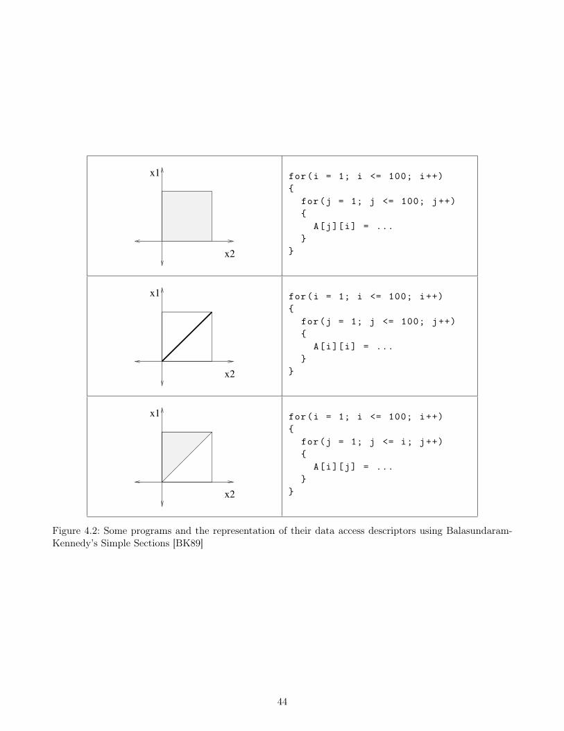
www.dedoimedo.com all rights reserved
x2
x1 for(i = 1; i <= 100; i++){
for(j = 1; j <= 100; j++){
A[j][i] = ...}
}
x2
x1 for(i = 1; i <= 100; i++){
for(j = 1; j <= 100; j++){
A[i][i] = ...}
}
x2
x1 for(i = 1; i <= 100; i++){
for(j = 1; j <= i; j++){
A[i][j] = ...}
}
Figure 4.2: Some programs and the representation of their data access descriptors using Balasundaram-Kennedy’s Simple Sections [BK89]
44
www.dedoimedo.com all rights reserved
cover some specific kinds of transformations because of coarseness of the dependence graph. It needs to beextended for statement level parallelism and for loop-nests greater than depth 2. Extension of their workwould also mean precise handling of parameters used in loop bounds because their input loop definitionscan only have fixed bounds and not parameters. Though they suggest that their model can be extended forsymbolic variables, it can easily be seen that the TVPI-ness is lost in such cases: {i+ j ≤ 10} is a UTVPIconstraint, while {i+ j ≤ N} is not. The latter has to be handled either by making some assumptions onN , or by an over-approximation or even by solving parametric UTVPI programs. Such special handlingof parametric variables is not needed in affine scheduling because it involves a solving a non-parametricpolyhedron obtained by application of Farkas lemma.
4.2.1.3 Our view of dependence over-approximations
Feautrier’s polyhedral approximation of dependences (as well as the more powerful DI abstraction) arereally different from the ones lower in the hierarchy because they can handle the parameters symbolically.A parameter can be considered a constant that is not known at compile time, which is not equivalent toconsidering it as an additional index-variable in several key problems, including linear programming andpiece-wise feasibility with respect to the parametric context. But the surprising fact is that Farkas-basedaffine transformations do not need to solve a parametric linear programming formulation at all. Henceit is clear that though solving parametric linear programs cannot be avoided for solving the dependenceanalysis problem, it can however be avoided for affine transformation algorithms using the Farkas lemmaor Vertex method. Such algorithms can use existing sub-polyhedra without the need for a parametricextension.
The view in this dissertation is that polyhedral abstractions like DP which include a provison forhandling parameters, should be used in loop transformations as they are extremely powerful to capturedomains, dependences and transformations in a single framework as well as being extremely rich to handlecomplex affine transformations like the ones mentioned above. The scalability problem should be tackledby proper algorithmic under-approximations of such a rich space rather than pre-determining either theinput dependence information or the type of transformations.
4.2.2 Creusillet’s approximations in array region analysis
Creusillet in her dissertation [Cre96]10 suggests multiple ways in which array region analysis can be done,while building theoretical frameworks—exact and approximate semantics—which are independent of theparticular representations and analyses. Specifically, she defines several types of array regions: READ andWRITE regions to summarize the effects of instructions and procedures; and IN and OUT regions thatrespectively contain the array elements imported and exported by the particular region.
Creusillet’s work is not in the context of program fragments in a restricted context like SCoPs [Fea91],but in more general and unstructured languages like FORTRAN, with even an interprocedural context.She notes that analyses that begin with dependence analysis in a restrictive language like SCoPs maybe quite costly; also, in spite of the preciseness that is possible, the limitatons may be too restrictive.
10We are thankful to Prof. François Irigoin who pointed us to the works in this section.
45

www.dedoimedo.com all rights reserved
Analysis in more general languages however, while having a much wider area of application, converselymay be cheaper. The goal of her work is to perform analyses like interprocedural dependence analysisusing READ and WRITE regions, and locality optimizations like array privatization using IN and OUTregions.
In this latter context, the traditional approaches have been to define may (resply. must) sets as over-(resply. under-)approximations of the exact solutions. Creusillet notes that under-approximations havebeen tried and found to yield trivial or uninteresting approximations. The main reason for this is thatwhen the chosen domain is not closed under set-union—including domains like convex polyhedra [Tri84],and weaker ones like Regular Section Descriptors (RSDs) [Cal87, CK88]—the under-approximations arenot uniquely defined. This directly means that, given an exact array region, no best under-approximationcan be defined. Over-approximation however can be uniquely defined. Moving to more general domains—like Presburger formulae—for under-approximations may lead to unscalable solutions. Wonnacott [Won95]reports the results of such an approach using Omega [Pug92, Pug91], but his analyses are limited to intra-procedural level; in an inter-procedural level, it is not known how such general domains would scale.
Creusillet [Cre96, Chapter 4] therefore proposes a method which uses both under- and over-approximateanalysis at the same time. Primarily, she proposes theoretical framework using Complete Partial Orders(lattice theoretic frameworks [CC77]) to define under- and over-approximations. This is followed by pro-posal of a computable exactness condition for checking whether a particular over-approximation is equalto the exact solution. In this latter case, the under-approximation need not be computed as the samesolution works as both over- and under-approximations. The advantage of the above work is that exactcomputation of the costly under-approximation is avoided, while at the same time, achieving the samethrough the exactness conditions.
The framework is part of the PIPS project [PIP], thanks to her extensive implementation. Experi-ments on large-size real-life applications lead to several loops containing procedural calls were successfullyparallelized, thanks to the algorithms suggested in her dissertation. Notable among the similar approachesis the work of Polaris [Tu95], where a similar approach has been applied using lists of RSDs. Further,Havlak’s work [HK91] is also with a similar theme.
The work in this dissertation is not directly comparable to Cresillet’s work; the former is about pro-grams in a restricted context, while the latter is in a more broader context. Also, the former is primarilyabout affine transformations for tiling and code-generation, while the latter is about the dependence analy-sis and optimizations like array privatization. Further, in the above work, there is no asymptotic reductionin the cost of analysis; this is mainly because convex polyhedra have been used as elements of the semanticframework in the implementation.
In spite of the above differences, her work has a positive inflence on this thesis. Her algorithms andimplementation have been tested extensively and offer interesting application perspectives for our work.Also, a sub-polyhedral domain like (U)TVPI polyhedra, along with supporting algorithms which find over-as well as under-approximations algorithms can augment the work; it could provide an improvement in theasymptotic compexity. This suggestion is because her work predates the more recent works of Miné [Min06]on UTVPI-polyhedra, and Simon et al. [SKH10]’s on TVPI-polyhedra. Further work is needed in making
46

www.dedoimedo.com all rights reserved
the two communities of static analysis and loop-transformation build from the other’s work.
4.2.3 Simplex Based Methods
4.2.3.1 Feautrier’s scalable and modular scheduling
Feautrier in his scalable and structured scheduling [Fea06] begins with a complexity estimate of affinescheduling, and concludes that affine scheduling methods which use cubic time simplex algorithm to solvethe linear programs for scheduling easily lead to algorithms with 6th power complexity in the number ofvariables in the input program11, making the parallelizer highly unscalable.
Feautrier hence proposes a modular specification language Communicating Regular Processors (CRP),an extension of C programming language, in which smaller systems or modules, comparable to functionsof C could be defined. The modules communicate with each other through inports and outports, andcommunication channels between two modules are multi-dimensional arrays. The modules in CRP systemcould be scheduled independently from each other, leading to smaller size simplex problems and hencebetter compilation times, almost linear in the number of modules in an input system. Feautrier alsoproposes search methods in which the original program could be decomposed into smaller systems. Clearly,the modules in CRP can be compared to systems of Alpha programming language [MQRS90, QR02] andto processes in Kahn Process Networks [Kah74]. Using the above CRP system, Feautrier reports theexecution times of usual schedulers, starting from tens of minutes and ending much longer. These longertimes concur with the ones we showed in Chapter 2.3.2 on page 11 using the PLuTo system.
To reduce the compilation times, Feautrier suggests several heuristic techniques. Like the earlier work ofFeautrier [Fea92a], the modular scheduling algorithm begins the simplification process of Farkas multiplierswith Gaussian elimination. Though the above step does not remove all the λ-multipliers which appear inequations, it is helpful to some extant. For elimination of all of the λ-multipliers, Feautrier suggests threeapproaches: Fourier-Motzkin, parametric linear programming and Minkowski decomposition. Feautriersuggests using Minkowski decomposition since an individual module is likely to be small, and this methoddoes not generate redundant constraints like the other two methods. This step has the advantage ofa redundancy elimination at an individual modular level, thereby contributing to a smaller number ofconstraints in the overall system.
The above steps leave a polyhedron with only µ-multipliers as variables. For solving the linear systeminvolving only these Farkas multipliers, Feautrier suggests stepwise scheduling, a heuristic modification ofthe simplex algorithm, linked with an elimination process which exploits the structure of the dependencegraph and hence the sparsity of the simplex tableau. He also suggests methods by which statements couldbe grouped together so that smaller simplex problems could be solved. All these steps lead to improvementsin the execution times of the scheduler.
11The discepancy between this 6th power and the 5th power estimate we made in Section 2.3.5 on page 16 is simply becauseof different heuristic estimates of Simplex algorithm. Both concur that affine scheduling involves solving an LP problem ofsize d|E| × d|V |. We assume optimistically that the latter is O(|E|2|V |) ≈ O(|V |5), while Feautrier assumes pessimisticallythat it is O(|E|3) ≈ O(|V |6). Though we presented some empirical evidence in Chapter 2 on page 7 followed by some morein the later Chapter 7 on page 89, further experimental validation of either of these complexity estimates, or even obtainingnew one, by doing experiments on simplex across wide range of benchmarks like PolyBench [PB+] needs to be done.
47

www.dedoimedo.com all rights reserved
These methods are complimentary to using sub-polyhedra based methods: they can be complimentaryto each other. Also, each of the individual steps in Feautrier’s method, namely elimination of λ-multiplierslocally, redundancy reduction, using the structure of dependence graph and grouping of statements cer-tainly are steps in the positive direction. However, the main limitations of the approach is that it does notguarantee any asymptotic improvement over existing methods. Also, it still needs to construct the simplextableau whose size O(mn) is quadratic in the size of the input system, and hence the input dependencegraph. This can be a serious limitation in JIT compilers with memory constraints. Further, there is achance that the optimizer loses its portability because it is tied to a particular simplex algorithm. Ideally,the parallelizer algorithm would like to use an out of the box implementation of simplex, like PIP [Fea88],and modifying the latter is an involved process.
4.2.3.2 Tuning the simplex algorithm
Another way of continuing to using Farkas based affine scheduling algorithms and still obtain a reductionin the time complexity, is to tune the simplex algorithm that is used for solving linear programs. Broadly,in this method, the simplex algorithm is made to run for a fixed predetermined number of pivots.12
As indicated earlier in Section 3.3.1 on page 28, we can assume that simplex usually takesO((m+n)mn)
observed time, with the number of pivots being always linear (O(m+n)) in number. These number of pivotscan be reduced to a constant number, meaning that the simplex algorithm is tuned so that it automaticallystops afterK number of pivots, whereK is an pre-determined constant, independent of eitherm or n. Withthis method, the observed complexity of simplex would be O(Kmn). If K is sufficiently small and fixed,like ten or so, then the overall complexity would be O(mn) which is not only small, but asymptotically thesame as Bellman-Ford as guaranteed by UTVPI polyhedra. Also, this method has the additional advantagethat it needs no further implementation than using a standard LP solver like PIP [Fea88] if the numberof pivots can be bounded.
More empirical evidence is needed, but the following are the a priori objections to the above method,which is a heuristic for the simplex, rather than methods based on Sub-polyhedra.
This method cannot be made to give a lexmin, and the solution picked up by the basic feasible solution(initial solution) and improved a little by the constant number of pivots may be quite bad for a schedule.
For use in a parallelizer which needs a theoretical worst-case complexity guarantee, complexity ofthe above method is closely linked with a simplex implementation which can provide such a support forconstant number of pivots. Though simplex implementation itself is fairly standard, a good implementationwhich can exploit sparsity, as well as provide good pivoting is quite an involved one. Compilers tend touse an out of box implementation provided by PIP [Fea88] or CPLEX [CPL] which do not have such aprovison and such kind of investment in the LP infrastructure may be underutilized by such heuristicfixing of the number of pivots.
Also, the method still takes a m × n = O(mn) space to construct and store the simplex tableau,and quadratic space can be quite heavy on the system. In spite of simplex algorithms taking various
12We thank Armin Größlinger for suggesting this approach at IMPACT-12 workshop as an alternative to our (U)TVPIbased methods.
48

www.dedoimedo.com all rights reserved
precautions about the table size increase by exploiting sparsity, our experience with PIP in our unscalabilityexperiments (in Chapters 2 on page 7, and Chapter 7 on page 89) is that the above memory requirement isquite heavy for large SCoPs, especially for ones with more than 1000 dependences, and using any tableaubased construction in JIT compilation could be unacceptable.
Further, we see below that using the (U)TVPI approximations can not only be applied to polynomialtime affine scheduling methods for better worst-case performance, but also have the potential to givepolynomial time approximate algorithms for loop scheduling problems that are NP-Complete. Also, ifduring code generation, integer vertices are needed, the UTVPI approximation can be tuned for that.These two problems cannot be solved with simplex based method(s) without paying the price of solvingILP programs. See Chapter 8 on page 101 for more details.
4.2.4 Other alternatives
To address this scalability challenge, we also consider some other existing alternatives for scalabilityproblem. First we cover two non Farkas-based methods, the vertex method [RPF86, QD89] and the Darte-Vivien’s method [DV97a] and then summarize Pouchet’s heuristics [Pou].
The Vertex method. The vertex method was the most general “pre-Feautrier” affine scheduling al-gorithm and was proposed by Rajopadhye et al. [RPF86] and Quinton and van Dongen [QD89]. In thismethod, non-linear constraints on schedule coefficients (as variables) are avoided by converting depen-dence constraints from the hyperplane to the dual vertex/ray representation (Minkowski decomposition).This process leads to a constraint system with too many variables and constraints: practical dependencepolyhedra are likely to have a very small hyperplane representation while having an exponential num-ber of vertices. The method has more scalability limitations than Farkas-based scheduling, as shown byFeautrier [Fea92a] and confirmed experimentally by Balev [BQRR98].
Darte-Vivien’s method. Darte and Vivien’s algorithm [DV97a], which relies on the DV abstractionwhich has been briefly summarized in the dependence abstractions section, is a non-Farkas method. Itinvolves one LP call per depth of the decomposition: O(Z) ≈ O(m2n) ≈ O(|E|2|V |) ≈ O(|V |5), if weassume the d, the depth of the decomposition tree to be bounded. Though it is likely that the gaussianeliminations of simplex algorithm terminate earlier for uniform dependences as evidenced in the slowerrate of growth for ITR-SEIDEL example when compared to the ITR-MATMUL example in Section 2.3.2 onpage 11, and there is even some empirical evidence [Mei96] to show that the running time of this algorithmis practically smaller than Feautrier’s method, this complexity is asymptotically the same as Feautrier’salgorithm,
Pouchet’s FM library and heuristics. The other notable approach which reduces the cost of solvingthe linear systems that arise in polyhedral compilation is implemented in Pouchet’s redundancy awareFourier-Motzkin (FM) library [Pou]. It has been known that Fourier-Motzkin has doubly exponentialcomplexity, though it empirically scales well [Pug92]. Though a detailed comparison is needed, we note
49

www.dedoimedo.com all rights reserved
Interval Over-Approximationof an Octagon
Miné’s UTVPIOver-Approximation of a
Polyhedron[Min06]
Simon et al.’s TVPIOver-Approximation of a
Polyhedron[SKH10]
Figure 4.3: Some Existing Sub-Polyhedral Approximations
that Pouchet’s method does not asymptotically reduce the complexity in a predictable way. Nevertheless, itis clear that the overall search space contains many valid yet useless transformations, and many redundantones in terms of generated code or behavior on the target platform. This is why we consider our work tobe complementary to the FM approach and the heuristics therein.
4.3 Some Existing Algorithms to Approximate into Sub-polyhedra
From the sub-polyhedral literature, we are not aware of any systematic study of under-approximationalgorithms. We however are aware of two algorithms on over-approximation. Here is a summary of them.Some more heuristic methods are listed in conclusions section.
4.3.1 Interval over-approximation
Interval over-approximation of an arbitrary polyhedron is a trivial approximation and has been assumedand solved many times in polyhedral literature.
For a system with n variables and m constraints, one can run 2n linear programs, twice per eachvariable xi, with the objective function being max(xi) and min(xi), each returning the upper-bound andlower-bound respectively of variable xi.
The above method is simple, and has cost 2nZ, which on average case takes O(m2n2) time, and couldbe quite affordable if n and m are small. Further, the method can use an existing simplex implementation.
But, it is likely that the above approximations are relatively uninteresting for a majority of programs.
4.3.2 UTVPI over-approximation by Miné
Miné [Min06, Section 4.3] proposes an algorithm to over-approximate a general polyhedron into a UTVPI-over-approximation. The algorithm however uses the generator representation and has the cost O(d2(|R|+
50
www.dedoimedo.com all rights reserved
|V |)), where d is the dimension and |R| and |V | are the number of rays and vertices respectively. It returnsthe tightest over-approximation-UTVPI of the given polyhedron.
Briefly, the method uses a greedy approach of incrementally building an Octagon, exploiting anotheralready developed algorithm to do convex union of two octagons and octagonalize the result. The over-approximation algorithm begins with an arbitrary vertex of the input polyhedron, which is trivially anOctagon and iteratively adds vertices to it, each time obtaining an incremental octagonal convex-hull forthat particular set of vertices which have been over-approximated. A similar procedure is repeated foreach ray of the polyhedron as well. The result of this algorithm is the tightest over-approximation for theinput polyhedron.
If the above algorithm of Miné is considered to be equivalent of Prim’s algorithm for finding minimumspanning tree for a directed graph in the sense of maintaining a single tightest UTVPI-OA polyhedronof the generators already approximated, it can even be adapted to run similar to Kruskal’s algorithm bymaintaining a forest of UTVPI-OAs [CSRL01] which can be incrementally coalesced to form the overallUTVPI-OA.
Needless to say, the method given as well as its variation suggested above use the generator represen-tation of the polyhedron which could be costly. We are aware of no efficient algorithm to directly computethe UTVPI over/under-approximations using only the constraint representation.
4.3.3 TVPI over-approximation by Simon-King-Howe
Simon, King and Howe [SKH10, Section 3.2.6] propose an algorithm to over-approximate a general poly-hedron into its TVPI-over-approximation.
Briefly, the approximates a constraint a1x1 + · · · + anxn ≤ c of a Polyhedron P using the set ofconstraints ajxj + akxk ≤ c− cj,k for every 1 ≤ j < k ≤ n. They propose that each cj,k can be calculatedas the result of a linear programming problem: cj,k = minExp(
∑i∈[1,n]\{j,k} aixi,OA(Pi)) and OA(Pi)
is the incremental over-approximation polyhedron obtained at the i’th step of computation. The abovestep13 needs to be iterated for each non-TVPI constraint of P .
For converting a general polyhedron with n variables andm constraints into a TVPI over-approximation,it can be seen that the above algorithm has cost n2m2Z, which in average case takes O(m4n3) ≈ O(n7)
time, assuming m = O(n). This could be quite expensive, unless n is very small.Further, the above method is hampered by unbounded variables in the original set of constraints. For
example the polyhedron {x, y, z|x+ y+ z ≤ 1} cannot be over-approximated by the above method as cj,kvariables are returned as unbounded variables each time in the calls to minExp.
Other than the above result, as far as we know, this process of efficiently over-approximation of ageneral linear program using TVPI constraints is an open problem.
13One way of looking at the above step is that it fills in cj,k entries into a lower-diagonal matrix of size n× n.
51
www.dedoimedo.com all rights reserved
4.4 A New Schema using Schedule Space Under-Approximation
In this thesis, we propose that the Farkas system P be Under-Approximated (UA) to improve the scala-bility of the scheduling algorithm. This means that instead of searching for an optimal feasible point inP , we search in Pa = UA(P ). The above approximation is legal and only leads to a conservative approx-imation of losing schedules, though it is well proven [PBB+11] that P is highly redundant with respectto schedule points. The overall process has to ensure that the approximation algorithm, as well as thesolution finding time be scalable algorithms. We can restrict these requirements further and say that bothof these algorithms should have worst-case strongly polynomial time running times matching the complex-ities of (U)TVPI sub-polyhedra introduced in Chapter 3 and summarized in Table 3.2 on page 30. Thepolynomiality is not a general restriction for the approximation algorithm, as one can separate the overallprocess of finding schedules into an offline and online process.
The above approximation can also be done on a per-dependence-edge basis. In this method, the per-dependence-edge Farkas polyhedra Pe are under-approximated, and the solution is found from the overallpolyhedron obtained by putting together all the per-dependence UAs. Namely, by doing
Pa = UA(P ) = ∩e∈EUA(Pe)
If the above approximation leads to a non-empty polyhedron, then we can find schedules using UA(P )
instead of P .In the above, we are exploiting the property that each of the individual Pe’s of polyhedral compilation
are guaranteed to be non-empty [Fea92a] directly as a result of dependence analysis. In polyhedral compi-lation, this property is true, as otherwise the statements corresponding to that particular dependence-edgecould as well be removed from the program as a form of dead-code elimination. It also helps that each ofthe per-dependence-edge Farkas polyhedra Pe are comparably much smaller than the overall polyhedron.This leads to the following direct approximation method:
A direct approximation method using UA into (U)TVPI sub-polyhedra.
1. Approximate each Pe into a (U)TVPI-polyhedron UA(Pe).
2. Build the complete constraint system by intersecting all the individual approximations: UA(P ) =
∩e∈EUA(Pe).
3. Solve the system UA(P ) using appropriate solution technique: Hochbaum-Naor’s technique [HN94]for TVPI polyhedra and Bellman-Ford for UTVPI polyhedra.
In Step 1 of the above method, as the individual constraint polyhedra (Pe’s) could be quite small, we couldeven use high complexity techniques. Step 2 of the above method is exactly as suggested by Feautrier andinvolves collating the under-approximated sub-polyhedral systems. Step 3 of the above method uses the(U)TVPI solution methods, like Fourier-Motzkin pruning of Hochbaum-Naor to determine the feasibilityof a TVPI linear systems and Bellman-Ford algorithm for UTVPI systems. Both these algorithms stronglypolynomial time algorithms (with O(mn2 logm) and O(mn) worst-case complexity respectively).
52

www.dedoimedo.com all rights reserved
We claim that a valid schedule can be determined using the above method in strongly polynomial time.It follows directly from the polynomial-time claims of under-approximation as well as the bounds of thesolution techniques.
Here is an alternative method in which a (U)TVPI-UA can be obtained.
Indirect under-approximation using duality. To obtain an sub-polyhedral under-approximation ofa rational polyhedron P , one can transform the polyhedron into the dual-space obtaining P ∗, and thenobtain the over-approximation of the dual-polyhedron OA(P ∗) and convert the over-approximated dualpolyhedron into primal space (OA(P ∗) → UA(P )) to get an under-approximation UA(P). In effect, wewill be doing P → P ∗ OA(P ∗) → UA(P ). The proof of these methods14 is trivial using a simpleconvexity argument on the polyhedra involved. This over-approximation15 can run on a per-dependenceedge basis as well.
For the above methods to work, each dual polyhedron P ∗e need be over-approximated by a min-cost-flow polyhedron, or even a generalized min-cost-flow polyhedron, as defined by Wayne [Way99]. This isbecause TVPI-polyhedra and min-cost-flow polyhedra are LP-duals of each other. The resultant over-approximation’s dual polyhedron will be a TVPI polyhedron.
The above procedures make the under-approximation and over-approximation as asymptotically com-parable methods, but for the transformation into dual-space. In case when the constraints/vertices of theinput polyhedron are too many, then the cheaper direct method could be used.
4.5 Scheduling using Under-Approximations: An Example
We illustrate the direct under-approximation approach on Feautrier’s one-dimensional scheduling [Fea92a,Example 1]16 which induces the following constraint system:
µ2,1 − µ2,2 − µ1,1 + µ1,2 = λ1,1 − λ1,2
µ2,3 − µ2,4 = λ1,3 − λ1,4
µ2,2 + µ2,4 − µ1,2 = λ1,2
µ2,0 − µ1,0 − 1 = λ1,0
After simplification by Gaussian elimination, followed by removal of λ-variables, the above becomes:
C1 : µ2,0 ≥ µ1,0 + 1
C2 : µ2,1 + µ2,4 ≥ µ1,1
C3 : µ2,2 + µ2,4 ≥ µ1,2
C4 : µ2,3 ≥ µ2,4 + 1
14These methods work only when 0 ∈ P. Otherwise, the polyhedra should be shifted so as to satisfy this condition. Wewill see in the next chapter how this complication can be avoided by using conical polarity.
15This over-approximation is not the same as the dependence over-approximation discussed in Section 4.2.1.1. Here, it isthe dual of the Farkas constraint system that is being over-approximated, while there, it is the dependence polyhedron thatis being over-approximated.
16The same example is also in Darte et al. [DRV00, Example 20, p. 220–222].
53

www.dedoimedo.com all rights reserved
Let us denote the sub-systems as P1 = {C1, C2, C3} from dependence D1 and P2 = {C4} from dependenceD2. It can be seen that the sub-systems P1 and P2 are not independent, sharing variable µ2,4 with eachother. Feautrier suggests two schedules to the above system.
• Schedule 1: Arbitrarily choose µ1,0 = µ1,1 = µ1,2 = µ2,1 = µ2,2 = µ2,4 = 0 and µ2,0 = µ2,3 = 1 whichleads to the schedules {θ(S1, i, N) = 0; θ(S2, i, j,N) = j + 1}.
• Schedule 2: This time, one can choose µ1,0 = µ1,2 = µ2,2 = µ2,4 = 0 and which leads to µ2,1 = µ1,1 =
1. The schedules are {θ(S1, i, N) = i; θ(S2, i, j,N) = i+ j + 1}.
Let us now study three sub-polyhedra and the impact on the affine schedules, in an increasing orderof expressiveness. All three systems are amenable to strongly polynomial algorithms to compute sched-ules. Though in this thesis, we do not use interval approximations, we begin with an interval under-approximation for the sake of exposition.
Interval under-approximation. Neither of the sub-systems P1 and P2 are Intervals. One can howeverunder-approximate each of them so that the resultant sub-systems are interval sub-polyhedra. Here is onepossibility among many others.
For P2, choose the under-approximation Interval(P2) = {µ2,3 ≥ 1, µ2,4 = 0} which is an interval. Thisleads to P1 having the system {µ2,0 ≥ µ1,0 + 1, µ2,1 ≥ µ1,1, µ2,2 ≥ µ1,2}, which is still not an interval. Onecan then choose {µ1,0 = 0, µ1,1 = 0, µ1,2 = 0} leading to
Interval(P1) = {µ2,0 ≥ 1, µ2,1 ≥ 0, µ2,2 ≥ 0}
The overall system is {µ2,3 ≥ 1, µ2,4 = 0, µ2,0 ≥ 1, µ2,1 ≥ 0, µ2,2 ≥ 0}. One solution of the system is {µ2,3 =
1, µ2,4 = 0, µ2,0 = 1, µ2,1 = 0, µ2,2 = 0}, which results in schedules {θ(S1, i, N) = 0; θ(S2, i, j,N) = j + 1},which is same as Schedule 1 by Feautrier[Fea92a].
UTVPI under-approximation. It can be observed that P2 is already a UTVPI. On the other hand, P1is “mostly” a UTVPI with constraint C1 already being a UTVPI needing no approximation, while C2 andC3 have to be under-approximated into UTVPI. To obtain the UTVPI under-approximation intuition, onecan observe that µ2,4 is a shared variable between the non-UTVPI constraints C2, C3 and UTVPI constraintC4. Since there is no other shared variable, we are free to choose any non-negative values to them, withouteffecting the others. The variable µ2,4 along with each of the pairs of variables {µ2,1, µ1,1} and {µ2,2, µ1,2},creates halfspaces passing though origin dividing their corresponding 3d-space accordingly. One can simplyset the value µ2,4 = 1 leading to UA(C2) = {µ2,1 + 1 ≥ µ1,1} and UA(C3) = {µ2,2 + 1 ≥ µ1,2}. Solving thissystem and choosing the other variables as µ1,0 = µ1,1 = µ1,2 = 1 and µ2,0 = µ2,1 = µ2,2 = 0 and leads tothe schedules {θ(S1, i, N) = 1 +N ; θ(S2, i, j,N) = j +N}.
TVPI under-approximation. Since P2 is already a UTVPI it is a TVPI as well, while P1 needsto be under-approximated into one. The above UTVPI under-approximations are valid as TVPI under-approximations well. This is true because each coefficients of constraints belong to {0,±1}.
54
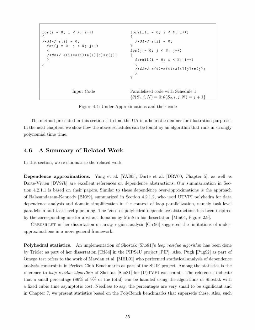
www.dedoimedo.com all rights reserved
for(i = 0; i < N; i++){/*S1*/ s[i] = 0;
for(j = 0; j < N; j++){/*S2*/ s(i)=s(i)+A[i][j]*x(j);}
}
forall(i = 0; i < N; i++){
/*S1*/ s[i] = 0;}for(j = 0; j < N; j++){
forall(i = 0; i < N; i++){/*S2*/ s(i)=s(i)+A[i][j]*x(j);}
}
Input Code Parallelized code with Schedule 1{θ(S1, i, N) = 0; θ(S2, i, j,N) = j + 1}
Figure 4.4: Under-Approximations and their code
The method presented in this section is to find the UA in a heuristic manner for illustration purposes.In the next chapters, we show how the above schedules can be found by an algorithm that runs in stronglypolynomial time time.
4.6 A Summary of Related Work
In this section, we re-summarize the related work.
Dependence approximations. Yang et al. [YAI95], Darte et al. [DRV00, Chapter 5], as well asDarte-Vivien [DV97b] are excellent references on dependence abstractions. Our summarization in Sec-tion 4.2.1.1 is based on their papers. Similar to these dependence over-approximations is the approachof Balasundaram-Kennedy [BK89], summarized in Section 4.2.1.2, who used UTVPI polyhedra for datadependence analysis and domain simplification in the context of loop parallelization, namely task-levelparallelism and task-level pipelining. The “zoo” of polyhedral dependence abstractions has been inspiredby the corresponding one for abstract domains by Miné in his dissertation [Min04, Figure 2.9].
Creusillet in her dissertation on array region analysis [Cre96] suggested the limitations of under-approximations in a more general framework.
Polyhedral statistics. An implementation of Shostak [Sho81]’s loop residue algorithm has been doneby Triolet as part of her dissertation [Tri84] in the PIPS4U project [PIP]. Also, Pugh [Pug92] as part ofOmega test refers to the work of Maydan et al. [MHL91] who performed statistical analysis of dependenceanalysis constraints in Perfect Club Benchmarks as part of the SUIF project. Among the statistics is thereference to loop residue algorithm of Shostak [Sho81] for (U)TVPI constraints. The references indicatethat a small percentage (86% of 9% of the total) can be handled using the algorithms of Shostak witha fixed cubic time asymptotic cost. Needless to say, the percentages are very small to be significant andin Chapter 7, we present statistics based on the PolyBench benchmarks that supersede these. Also, such
55

www.dedoimedo.com all rights reserved
statistics are still on the dependence polyhedra, without any over-approximation algorithms for constraintsor polyhedra that are not (U)TVPI.
Unscalability of affine scheduling. In the vast framework of affine scheduling literature, Feautrier’sapproach in his scalable and modular scheduling [Fea06] is the closest to our approach in Section 4.4 andis a proper predecessor. Feautrier himself builds from his earlier work on scheduling [Fea92a] by properlydefining and addessing the scalability problem and suggests some methods by which it can be alleviated.The questions raised there as well as its positive influence on our work cannot be under-estimated. Thenew scheme that we introduced in Section 4.4 builds from his work, and we consider both contributions ascomplementary to each other. But, it should be noted that any future work that attempts to couple boththese techniques should be aware of the (mutual) limitation that simplex based methods do not preservethe (U)TVPI-ness of the constraint matrix because of the way gaussian eliminations—the main engineof simplex algorithm—operate: a gaussian elimination algorithm on a TVPI matrix normally destroys itsTVPI-ness.
Approximations of polyhedra. We are not aware of any previous algorithm for finding low-complexityapproximations of general polyhedra into sub-polyhedra other than finding the interval (“box”) polyhedralOAs. The literature is scarce about polyhedral approximations and more so for UAs. The naïve methodof projecting out some dimensions using a method like Fourier-Motzkin gives an over-appoximation, andat a very high time complexity.
Miné [Min06, Section 4.3] adapts the vertex method for finding the UTVPI-OA of a general poly-hedron. Simon et al. [SK10, Section 3.2.6] propose an iterative algorithm for the TVPI-OA of a generalpolyhedron using Linear Programming. We have summarized these algorithms briefly in Section 4.3. Vivienand Wicker [VW04] propose an algorithm to find the parallelepiped-OA of a 3d-polyhedron in vertex rep-resentation. Howe and King [HK09, Section 4.4] propose using a heuristic “projection based method” toapproximate a finite set of Poly constraints into Logahedra constraints using TVPI as intermediate step.More details are not given.
Kanade et al. [KAI+09] propose a heuristic method of finding the bounded vertex representation of apolyhedron by converting its representation to generator form, and throwing away some vertices, therebyobtaining an under-approximation. Colón and Sankaranarayanan [CS11, Section 5] as part of extendingtheir earlier work on template polyhedra [SSM04, SSM05] also suggest using under-approximations, justlike the above mentioned work of Kanade et al. [KAI+09]. Both the above works primarily need over-approximations like many other works of static analysis, but algorithmically solve the under-approximationproblem by convering into the polar space.
Kelly et al.’s work on transitive closure [KPRS96] also could be considered to be a polyhedral under-approximation of the transitive closure problem which is defined on general presburger arithmetic. Thislatter problem, though being undecidable in general, has a wide range of applications and many of themin parallelism, like determining the redundancy of inter-processor synchronizations.
56
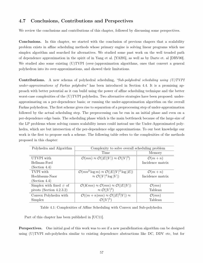
www.dedoimedo.com all rights reserved
4.7 Conclusions, Contributions and Perspectives
We review the conclusions and contributions of this chapter, followed by discussing some perspectives.
Conclusions. In this chapter, we started with the conclusion of previous chapers that a scalabilityproblem exists in affine scheduling methods whose primary engine is solving linear programs which usesimplex algorithm and searched for alternatives. We studied some past work on the well treaded pathof dependence approximation in the spirit of in Yang et al. [YAI95], as well as by Darte et. al [DRV00].We studied also some existing (U)TVPI (over-)approximation algorithms, ones that convert a generalpolyhedron into its over-approximations, and showed their limitations.
Contributions. A new schema of polyhedral scheduling, “Sub-polyhedral scheduling using (U)TVPIunder-approximations of Farkas polyhedra” has been introduced in Section 4.4. It is a promising ap-proach with better potential as it can build using the power of affine scheduling technique and the betterworst-case complexities of the (U)TVPI polyhedra. Two alternative strategies have been proposed: under-approximating on a per-dependence basis; or running the under-approximation algorithm on the overallFarkas polyhedron. The first scheme gives rise to separation of a preprocessing step of under-approximationfollowed by the actual scheduling step. The preprocessing can be run in an initial phase and even on aper-dependence edge basis. The scheduling phase which is the main bottleneck because of the large-size ofthe LP problems whose solving causes scalability issues could instead use the Under-Approximated poly-hedra, which are but intersection of the per-dependence edge approximations. To our best knowledge ourwork is the first to propose such a scheme. The following table refers to the complexities of the methodsproposed in this chapter:
Polyhedra and Algorithm Complexity to solve overall scheduling problemTime Memory
UTVPI withBellman-Ford(Section 4.4)
O(mn) ≈ O(|E||V |) ≈ O(|V |3) O(m+ n)Incidence matrix
TVPI withHochbaum-Naor(Section 4.4)
O(mn2 logm) ≈ O(|E||V |2 log |E|)≈ O(|V |4 log |V |)
O(m+ n)Incidence matrix
Simplex with fixed # ofpivots (Section 4.2.3.2)
O(Kmn) ≈ O(mn) ≈ O(|E||V |)≈ O(|V |3)
O(mn)Tableau
Convex Polyhedra withSimplex
O((m+ n)mn) ≈ O(|E|2|V |) ≈O(|V |5)
O(mn)Tableau
Table 4.1: Complexities of Affine Scheduling with Convex and Sub-polyhedra
Part of this chapter has been published in [UC11].
Perspectives. One initial goal of this work was to see if a new parallelization algorithm can be designedusing (U)TVPI sub-polyhedra similar to existing dependence abstractions like DC, DDV etc, but for
57
www.dedoimedo.com all rights reserved
multi-core architectures. The motivation of the above is the wide success of the FCO algorithm of Grieblet al. [GFG02] as implemented in PLuTo [BHRS08] with coarse-grain parallelization objectives. It still facesthe same scalability problems as Feautrier’s algorithm [Fea92a]. Such algorithm are similar to Wolf-Lam’salgorithms [WL91a, WL91b], though using Balasundaram-Kennedy’s simple sections abstraction [BK89],each of which were shown to be limited in scope.
Certainly, as pointed out by Yang et al. [YAI95], the previous dependence abstractions were tunedeither for a particular kind of input programs, or for a particular kind of transformations. But, none ofthese were designed with scalability objectives as part of design considerations. Balasundaram-Kennedy’ssimple sections [BK89] comes under the same category, and though the authors hint at scalability asan objective it misses out the opportunities offered by affine scheduling. Hence, the study showed thatre-adaptation of existing dependence methods by restricting the types of input is limited in scope17.
Hence, a new scheme using (U)TVPI-UAs of Farkas polyhedra has been proposed in Section 4.4. Sucha scheme is more powerful than the existing methods because of our ground in affine scheduling framework,and the use UA of Farkas polyhedra. But, we must also design scalable algorithms for constructing the(U)TVPI-UAs of general polyhedra. This is explored in the next two chapters, by first developing anunder-approximation framework in Chapter 5 followed by proposing new under-approximation algorithmsin Chapter 6.
17A possible open problem here is to design a parallelization algorithm similar to Lim and Lam’s synchronization freetechniques which uses affine transformations [LL97], though using (U)TVPI sub-polyhedra with a goal of acheiving scalability.
58
Chapter 5
A Framework for (U)TVPIUnder-Approximation
5.1 Introduction
In this chapter, we define a simple and sound mathematical background to build (U)TVPI under-approximationsof polyhedra, to linearize the problem of finding approximations, and to prove that the algorithms weconstruct in later chapters return valid approximations. To give these sufficient conditions, we take twoapproaches: an intuitive and geometric explanation using duality/polarity in Section 5.4, followed by amore direct way using the equivalent Farkas lemma in Section 5.5.
Starting with a polyhedron given in constraint form as P = {x|Ax + b ≥ 0}, we show that simpleunder-approximations of P can be obtained by reasoning about over-approximations of the dual (polar),associated with the transpose matrix [A |b]T . To accomplish the above, in Section 5.2 and Section 5.3,we introduce some basic lemmas about convexity like homogenization and polarity. Next, in Section 5.4,we construct a simple framework for reasoning about under-approximations and over-approximations in aunified manner. Finally, in Section 5.5, we show how the above construction could be used to define a per-constraint approximation scheme which helps to obtain TVPI approximations of the non-TVPI constraintsin the input polyhedron. The reader is referred to standard books for a complete coverage [Sch86, Zie06].
5.2 Some Background in Convexity
The overall goal of this section is to introduce some convexity concepts and relate them to TVPI under-approximations. Much of the math here is presented from standard books [Sch86, Zie06].
5.2.1 Homogenization
Homogenization can be done on Polyhedra in H-form (constraint form) or in V-form (vertex form orgenerator form). The following definition is when P is in H-form.
59

www.dedoimedo.com all rights reserved
Definition 5.2.1 [Homogenization]. Let P = P (A,b) (P = {x|Ax + b ≥ 0}) be a H-polyhedron,then its homogenization is a cone and also a H-polyhedron:
homog(P ) =
((A b
0T 1
),
(0
0
))= C(P ) (5.1)
A similar reverse operation dehomog can be defined for the reverse operation of de-homogenization.It can be noted that if A is am×n-system (m constraints and n variables), and b is am×1-vector, then
the homogenized constraint system C (or homog(P )) is of size (m+ 1)× (n+ 1). Note that the constantsdimension has become an additional dimension in the (n + 1)-dimensional space. We would be referringto this dimension as homogenizing dimension and the other dimensions as non-homogenizing dimensions.Also note that homogenizing is a process that can be reversed by special marking of the dimensions. Itshould also be noted that homogenization is a rather trivial process, which can be constructed in lineartime, and routinely done so in libraries like PIP/PolyLib. It however needs to be mentioned because thiswork deals with (U)TVPI constraints, which are defined to be having at most two non-zero coefficients inthe non-homogenizing dimensions.
5.2.2 Polarity and conical polarity
The following is the definition of polar of a polyhedron.
Definition 5.2.2a [Polarity]. For P ⊆ Rd, the polar set is defined by:
P ∗ ={c ∈ (Rd)∗ : cx ≤ 1 for all x ∈ P
}⊆ (Rd)∗
In standard books like Schrijver [Sch86], some of the theorems of polarity assume that the origin isan internal point of a polyhedron, namely that 0 ∈ int(P ). For ease of notation, we use subscript o todenote that kind of pre-supposition on the polyhedra: Po is a polyhedron such that 0 ∈ int(P ). Thepolyhedron which satisfies this restriction can be expressed in H-form as Po = {x|Ax + b ≥ 0;b ≥ 0}.Note the additional non-negativity restriction on b.
A polyhedral cone C, however, because 0 ∈ C, by definition.
Definition 5.2.2b [Polarity Properties: Polyhedra]. For P ∗o ∈ Rd, whose vertices are columns ofthe matrix V and whose rays are the columns of the matrix Y , the following are equivalent:
P ∗o = conv(0, V ) + cone(Y )⇐⇒ Po ={x ∈ Rn|V Tx ≤ 1;Y Tx ≤ 0
}The above correspondences give rise to some well known polarity properties namely that: the vertices(respectively, edges, and facets) of the primal correspond to the facets (respectively, ridges, and vertices)of the polar. (A facet is a (n−1)-dimensional face.) Furthermore, the constraints of a polyhedron correspondto vertices/rays of the polar. We use these correspondences in the proofs of this dissertation.
From the above, we can easily derive the following definition of the polar of a cone C:
60

www.dedoimedo.com all rights reserved
Definition 5.2.2c [Conical Polarity]. For C ∈ Rn, the polar set is defined by
C∗ = {c ∈ (Rn)∗ : cx ≤ 0 for all x ∈ C} ⊆ (Rn)∗
5.2.3 Polarity, (U)TVPI and (U)TCPV
A polyhedron can be represented in either of H-form or V-form. But, polyhedra that occur in polyhedralcompilation are almost always described in H-form. This means that the polar can be described, using astraightforward linear time construction, in V-form. Converting the primal to V-form or the polar to H-form is however costly as it involves a call to Chernikova algorithm which has exponential time complexity.In the following lemma, we implicitly use the above dual interpretation, without making an actual callto Chernikova. This dual interpretation is different from the dual representation in libraries like PolyLib,where a polyhedron (in either primal or dual space) is described using both H-form and V-form.
Note that in the above lemma, as we are using H-form (U)TVPI in primal, it implies that by astraightforward construction, the polar is in V-form.
Lemma 5.2.3 [(U)TVPI and (U)TCPV]. For a TVPI-polyhedron, the polar has vertices and rayswhich have not more than two non-zero components in the non-homogenizing dimensions. For a UTVPI-polyhedron, the polar has vertices and rays which have no more than two non-zero components each in thenon-homogenizing dimensions. The components belong to {−1,+1}. We define the polar of a (U)TVPIconstraint as (Unit-)Two-Components-Per-Vector or (U)TCPV vector. Further, we define the polar of a(U)TVPI polyhedron as a (U)TCPV polyhedron.
5.3 Polarity and Approximations
5.3.1 Polar of polar
The proofs of the following can be found in Schrijver [Sch86] and hence are omitted.
Lemma 5.3.1a [Polar of Polar and Equality]. (i) (P ∗o )∗ = Po, (ii) (P ∗)∗ = P ∪ {0}, and (iii)(C∗)∗ = C.
The proof of the following is straightforward (almost obvious), but we do it for completeness.
Lemma 5.3.1b [Polarity and Inclusivity]. For any two polytopes Po and Qo, Po ⊆ Qo ⇔ P ∗o ⊇ Q∗o.
Proof:
• To prove this, assume that Po is expressed in V-form and Qo in H-form. Let Po = conv(0, VP ) andlet c ∈ VP be an arbitrary vertex of Po. Further, let Qo = {x ∈ Rn|V T
Q∗ox ≤ 1} (this definition of Qo
in H-form is possible because of only-if part of Definition 5.2.2b). Because of the inclusivity in theif-direction Po ⊆ Qo, we have that V T
Q∗oc ≤ 1 is true. Comparing this latter with the definition of
Polar of Po, P ∗o = {c ∈ (Rd)∗ : cx ≤ 1 for all x ∈ Po} ⊆ (Rd)∗, by Definition 5.2.2a), we infer that
61
www.dedoimedo.com all rights reserved
all the vertices of Q∗o are enclosed by an arbitrary inequality of P ∗o . Since the same method can beiterated for any of the vertices of Po, we have that P ∗o ⊇ Q∗o.
• This proof part is similar to the “if part”, but assuming that P ∗o is expressed in V-form and Q∗o inH-form.
The above lemmas can obviously be extended for any general polyhedra and for cones as well.
Lemma 5.3.1c [Polarity and Inclusivity]. For any two cones K1 and K2, K1 ⊆ K2 ⇔ K∗1 ⊇ K∗2 .
5.3.2 Under-Approximation and Over-Approximation
The following corollary can be derived from the above lemmas.
Corollary 5.3.2 [Toggling between OA and UA]. (i) (OA(P ∗o ))∗ ⊆ Po, and (ii) (OA(C∗))∗ ⊆ CThe above corollary means that by taking the polar of a polyhedron and taking the resultant’s Over-
Approximation (OA) one obtains a polyhedron whose polar is an UA of the original polyhedron. Hence,the first half above corollary can be used to find the UA of a polyhedron by converting into polar spaceand taking the OA of its polar polyhedron.
5.4 A Construction for Under-Approximation
Using the theorems of the previous section, one can reason about UA by talking about OA in the dual/polarspace. But, using OA to find valid UA using duality-properties, means that one has to deal with the manycases of the polyhedron being bounded or not, whether it is homogenized or not (like in Lemmas 5.3.1),and whether origin is an internal point or not (like in Corollary 5.3.2.i). Further, the Farkas constraintpolyhedra (even the per-dependence ones) that are obtained in polyhedral analysis do not necessarily havethe origin as an internal point. Also, they are never bounded. So, we need a single framework to deal withall these cases.
In this section, we create a simple construction, using which the problem of finding a UA of a polyhedronin H-form is reduced to the problem of finding a OA of its polar cone in V-form. The construction useshomogenization and conical polarity and handles all the above cases in a unified and simple manner.The construction is the mathematical framework that gives us the basis to prove that the UAs we laterconstruct in Chapter 6 are valid approximations.
The super-scripts H and V show whether the particular polyhedron is in constraint or generator formrespectively.
PH homog−−−−−→ CH polar−−−→ KV OA−−→ KVa depolar−−−−−→ CHa dehomog−−−−−−→ PHa
The following is some notes on the above construction:
• [Step 0] PH: Input P , the Polyhedron to be under-approximated in H-form.
62
www.dedoimedo.com all rights reserved
• [Step 1] PH homog−−−−−→ CH: Compute Cone C by homogenizing P . Namely, C = Homog(P ). C is a conein H-form.
• [Step 2] CH polar−−−→ KV : Compute K = C∗, the Polar cone of the cone C. K is a cone in V-form.
• [Step 3] KV OA−−→ KVa : Compute Ka, the Over-Approximation of K such that K ⊆ Ka. Ka is a conein V-form.
• [Step 4] KVa depolar−−−−−→ CHa : Take the polar cone (DePolar) of Ka to result in Ca, which will be a conein H-form.
• [Step 5] CHa dehomog−−−−−−→ PHa : Dehomogenize18 Ca to result in Pa, which will be a Polyhedron in H-form.
In Step 0, P could be a general polyhedron in H-form, possibly in non-minimal form (having redundantconstraints). Step 1 follows from Definition 5.2.1. Here, the dimensions have to be marked as homogenizingand non-homogenizing dimensions so that it can help in approximation (Step 3), as well as in the de-homogenization (Step 5) later. No new homogenization is needed for performing this step other than whatis performed in standard libraries. As mentioned above, this is needed in particular because the subject ofthis dissertation is (U)TVPI systems, which by definition cannot directly operate on cones without thisspecial marking. Step 2 follows from Definition 5.2.2.
In the approximation process in Step 3, the Over-ApproximationKa has to satisfy (U)TCPV properties,so as to respectively obtain the (U)TVPI approximation of P . More particularly, for Ka to be a TCPVover-approximation of K, it should have not more than two non-zero components in the non-homogenizingdimensions. Further, for Ka to be a UTCPV over-approximation of K, Ka should be a TCPV vector andthe non-zero components should be from {−1,+1} (Lemma 5.2.3). In the approximation, one can neitherthrow away the offending dimensions, nor can throw away the offending vectors themselves (ones thatare not (U)TCPV), as the remaining vectors may result in an under-approximation of P . If K is beingapproximated on a per-constraint basis, the OA process could be such that Ka has multiple vectors foreach vector of K. The result of Step 3 is Ka = OA(K). Steps 4 and 5 are reverse of Steps 2 and 1respectively.
In the above, Pa (respectively Ca and Ka) are approximations of P (respectively C and K). Moreparticularly, we have the following theorem:
Theorem 5.4 [Approximations and the UA-OA Construction]. Let P be a polyhedron definedin H-form. Let C = Homog(P ), K = C∗, Ka = OA(K), Ca = K∗a , and Pa = DeHomog(Ca). Then, wehave: (i) Ka ⊇ K, (ii) Ca ⊆ C and (iii) Pa ⊆ P .
Proof: In (i) Ka = OA(K) by definition. In (ii), Ca = UA(C), because of Corollary 5.3.2.ii. Finally, in(iii) Pa = UA(P ) because of Corollary 5.3.2.i.
18We refer dehomogenizing as the reverse of Definition 5.2.1 (Equation 5.1 on page 60).
63
www.dedoimedo.com all rights reserved
The above construction algorithm can be done in linear time and can be considered to be a reinter-pretation of the input polyhedron in H−form so that the validity of the UA can be proved, and simplescalable algorithms could be obtained for (U)TVPI approximation. In the above algorithm, using homog-enization requires the origin to be an internal point. And, using polarity reduces the UA problem to theOA problem. But, one cannot swap the two steps of homogenization and polarity (swapping Steps 1 and2 and following it by swapping Steps 4 and 5), for example, by taking the polar of P and then taking theresultant’s homogenization. Doing so means that one has to “chop away” the origin from the polar of theresultant’s OA as in Lemma 5.3.1a.ii. Such a process involves the generator representation and is costly.
Observe that K in the above construction is in V-form. Its generator vectors are columns of thefollowing matrix:
K = cone
(AT 0
bT 1
)(5.2)
In matricial form, K is of size (n+ 1)× (m+ 1). K could thus be seen to be a transpose of Equation 5.1on page 60. K can also be written as the following:
K = cone
{(aT1b1
), . . . ,
(aTjbj
), . . . ,
(aTm
bm
),
(0
1
)}(5.3)
The objective of Step 3 remains to find the TCPV-OA of Polyhedron K given in V-form. This problemcan be seen as trying to find a cone Ka such that:
K ⊆ cone (Ka) (5.4)
By this Equation 5.4, if each column of K can be written as a conical sum of the vectors in Ka, thenthe approximation remains a valid approximation. If each vector in Ka is a TCPV vector, then thecorresponding Pa would be a TVPI approximation of P .
The alternate to the above scheme is to use conical polarity.
A simplification using conical polarity. From the definitions given in previous section, K, the polarcone corresponding to P can directly be constructed from homog(P ) in Equation 5.1 on page 60, and itsgenerator vectors are columns of the following matrix:
K = cone
(AT 0
bT 1
)
We would still need the
(0
1
)augmentation because of preservation of lineality space of the primal in
the polar. From the above, if we let Pa (respectively Ka) be the approximation of P (respectively K), wehave the following equivalence:
Ka ⊇ K ⇔ Pa ⊆ P (5.5)
64
www.dedoimedo.com all rights reserved
From which follows Equation 5.4 and the explanation therein.
5.5 Approximation Scheme for TVPI-UA using TCPV-OA
In this section, we formulate the sufficient conditions to prove that the UAs we later construct in Chapter 6are valid approximations. In fact, with the Farkas lemma in Section 2.2 on page 9 and the equivalenthomogenization-polarity construction in Section 5.4, we do have all the necessary ammunition to constructan approximation scheme which allows us to built TVPI-UAs of general polyhedra. UTVPI-UAs are simpleextensions of the material in this section.
In the rest of this section, for ease of exposition, we assume that the polyhedron P is in 3-dimensions(n = 3)19. The latter polyhedra, also called as 3VPI polyhedra, are general enough to represent anyarbitrary polyhedron. For polyhedra that are not 3VPI, a reduction exists that transforms any arbitrarypolyhedron into its equivalent 3VPI polyhedron.
According to Shostak [Sho81], the transformation from general convex polyhedra to 3VPI polyhedrais said to have been suggested by R.Tarjan and is very similar to the reduction of an arbitrary n-variableboolean satisfiability (“SAT”) problem to a 3SAT problem. This transformation is not an approximation,which is the subject of this chapter. Here is an example to illustrate the reduction.
Example 5.5 [Reduction from convex polyhedra to 3VPI]. The constraint w + x+ y + z ≤ 1 isobviously not 3VPI. It can be seen to be equivalent to the system {w + x ≤ v;w + x ≥ v; v + y + z ≤ 1}which is 3VPI. �
Note that the UA algorithms we present do not need to this reduction. We use it only to showequivalence.
Let the j-th column of K, with 1 ≤ j ≤ m, be Kj =(aj,1 aj,2 aj,3 bj
)T. Then we have
Kj =
aj,1
aj,2
aj,3
bj
∈ cone
tj,11 tj,12 0
tj,21 0 tj,230 tj,32 tj,33pj1 pj2 pj3
= cone(T j) (5.6)
It can be noticed that each column of the matrix T j is a TCPV vector and hence when it is subjectedto the reverse transformation of Steps 4 and 5 as discussed in Section 5.4, yields a set of TVPI constraints.The above is what we call as an approximation scheme. In this scheme,
Definition 5.5 [Approximation scheme]. A non-TVPI constraint aj,1x1 + aj,2x2 + aj,3x3 + bj ≥ 0
in the original system is replaced by the set of constraints UA(x1, x2, x3) = {tj,11 x1 + tj,21 x2 + pj1 ≥0; tj,12 x1 + tj,32 x3 + pj2 ≥ 0; tj,23 x2 + tj,33 x3 + pj3 ≥ 0}.
19It should be clarified that the n here refers neither to the number of elements in the constraint, nor to the number ofelements in the polar vector. It just refers to the dimension of the primal. In such a case, the number of significant elementsin the constraint and dual-vectors is n+ 1.
65
www.dedoimedo.com all rights reserved
In the above approximation scheme, every column vector of K which has more than two non-zerocomponents is replaced by a set of TCPV vectors, such that the original vector remains in the conicalsum of the replacements. The conical combination of the replacement vectors is an OA of the originalvector Kj . The above scheme remains valid as long as the (t, p) variables and the (a, b) constants satisfythe convexity requirement. One way for ensuring the same is by making the (t, p)-variables satisfy thefollowing additional constraints, which we would be referring to as context constraints for reasons that willbe exposed later:
tj,11 +tj,12tj,21 +tj,23
tj,32 +tj,33pj1 +pj2 +pj3
=
aj,1
aj,2
aj,3
bj
(5.7)
When such a set of Tj matrices is defined for each vectorKj ofK, then, we haveKa = cone{T 1, T 2, . . . , Tm
}and the resultant TCPV approximation would be K ∈ cone
{T 1, T 2, . . . , Tm
}. With the above, we give
the following theorem, whose proof builds on Theorem 5.4 and the arguments given in this section.
Theorem 5.5 [TVPI and UA]. Let Pa be the polar of the Ka vectors obtained in Equation 5.7. Then,Pa is a valid TVPI-UA of the original Polyhedron P .
Proof: We employ the affine form of Farkas lemma, with the premise of non-emptiness of P guaranteedbecause of the per-constraint method. For the UA to be proper, the affine form corresponding to theoriginal constraint ajx + bj should be expressible as a positive sum of the replacement TVPI vectors
aj,1x1 + aj,2x2 + aj,3x3 + bj
≡ λj0 + λj1(tj,11 x1 + tj,21 x2 + pj1) + λj2(t
j,12 x1 + tj,32 x3 + pj2) + λj3(t
j,23 x2 + tj,33 x3 + pj3)
where the λ-multipliers satisfy λj0, λj1, λ
j2, λ
j3 ≥ 0. Pairwise matching for each of the x-variables yields:
aj,1
aj,2
aj,3
bj
=
λj1t
j,11 +λj2t
j,12
λj1tj,21 +λj3t
j,23
λj2tj,32 +λj3t
j,33
λj0 +λ1pj1 +λj2p
j2 +λj3p
j3
(5.8)
Setting λj1 = λj2 = λj3 = 1 yields the context constraints defined in Equation 5.7 proving the validity ofthe approximation, except for the additional λj0 in the homogenizing-dimension-matching. Setting λj0 = 0
is safe, and we will see later that it actually contributes to the quality of the approximation. �
The problem remains to find such a set of (t, p) variables satisfying the above context constraintsEquation 5.7, so that the approximation remains valid. It can be seen that searching for the (t, p) variablesdirectly could lead to a non-linear (quadratic) formulation. Even searching for t-variables that satisfy theabove constraints turns out to be non-linear. But, as they are existentially quantified, the equations be
66

www.dedoimedo.com all rights reserved
solved using advanced quantifier elimination techniques like [Tar51], which are well known to be unscalablebeyond small inputs and certainly not polynomial.
In the next chapter however, we propose some linearizations of the above mentioned approximationscheme, so that the approximation algorithms remain scalable. This is done first as a heuristic where both(t, p)-variables are arbitrarily fixed, and then as a more formal method where only the t-variables are fixed,while the p-variables are found by an LP formulation.
67

www.dedoimedo.com all rights reserved
non−TCPV
TCPV
TCPV
TCPV
j
k
i
i−jj−k
k−i
Figure 5.1: An illustration of TCPV approximation of a non-TCPV general vector
5.6 Conclusions
In this chapter, we use a simple framework based on polarity and showed that it can be used for designingthe Under-Approximation algorithms. We also studied a direct application of Farkas lemma as an alternateto the framework, which achieved the same very concisely20. A more detailed presentation of this materialcan be found in [UC11, UC12]. An illustration of the duality construction is shown in Figure 5.1.
Three equivalent alternatives: This chapter showed three alternate ways of obtaining under-approximationsthrough the use of duality: by the use of a homogenization-polarity construction, use of conical polarityand Farkas lemma. Each of these are equally powerful to the other and show that there are many alternateways of looking at our scheme and proving its validity.
This chapter is closely tied with the algorithms presented in the next chapter. So, more detailedconclusions and perspectives are offered after covering the algorithms.
20We thank Paul Feautrier and Armin Größlinger for suggesting this proof simplification.
68
Chapter 6
Polynomial Time (U)TVPIUnder-Approximation Algorithms
6.1 Introduction
In this chapter, we use the framework developed in Chapter 5 and develop worst-case polynomial timealgorithms for obtaining (U)TVPI under-approximations of polyhedra. Firstly, in Section 6.2, we give astrongly polynomial time per-constraint algorithm for TVPI-UA. Then, in Section 6.3, we give an LP basedper-constraint weakly polynomial time algorithm for TVPI-UA. In Section 6.4 we propose various waysin which the above LP based algorithm can be applied when multiple non-TVPI constraints are present.In Section 6.5, we give a strongly polynomial algorithm that gives a UTVPI-UA of a TVPI polyhedron.In Section 6.6, we briefly sketch a parametrized UTVPI-UA approximation method. In Section 6.7, wediscuss the metrics and complexity of the algorithms. Finally, in Section 6.8, we conclude with a summaryof the contributions, and discuss some perspectives.
6.2 The Median method for TVPI-UA
In this section, we introduce a simple per-constraint heuristic using the framework developed in Sections 5.4and 5.5. The main idea of this approximation is Equation 5.4 on page 64, which states that the originalvector can be approximated by any set of the replacement TCPV vectors, as long as the former remainsin the cone of the latter.
Definition 6.2 [Median method: 3-d case]. The inequality ax+by+cz+1 ≥ 0 can be approximatedby the set of inequalities {ax+ by + 2
3 ≥ 0; ax+ cz + 23 ≥ 0; by + cz + 2
3 ≥ 0; }.Geometric intuition for the above derives from the observation of the polar space, where the above
69
www.dedoimedo.com all rights reserved
approximation is the following: a
b
c
1
∈ cone
12a
12a 0
12b 0 1
2b
0 12c
12c
13
13
13
The intuition for the above approximation comes from Equation 5.6 on page 65. In that equation, the
values of t-variables and p-variables satisfy Equation 5.7 on page 66; such assignments have to be foundout to obtain an approximation. As explained in Chapter 5, the t-variables have to be determined by achoice so that linearity is satisfied. The method in this section fixes the p variables also in a heuristicmanner by dividing the available “budget” in the homogenizing dimensions equally between the values inthe homogenizing dimensions of the replacement TCPV vectors. This is not the only way for obtaining anapproximation. It is one of the many ways, which is intuitive and builds the platform for more powerfulunder-approximations that we will see in later sections. We call this the median method because theoriginal vector is the median of the replacement vectors in the polar space.
4-d case. For illustration purposes, the approximation is the following for 4d case
a
b
c
d
1
∈ cone
13a
13a
13a 0 0 0
13b 0 0 1
3b13b 0
0 13c 0 1
3c 0 13c
0 0 13d 0 1
3d13d
16
16
16
16
16
16
General n-d case. The above can be easily be generalized to n-d polyhedra. Let s be the sparsity ofa polyhedron, i.e., the number of non-zero variables (outside the homogenizing dimension) for a specificconstraint, with 1 ≤ s ≤ n. Let q =
(s2
)= s(s− 1)/2 and let r = s− 1. The resultant set of TCPV vectors
corresponding to the particular constraint are n+1 dimensional, with cardinality q. The coefficients of thenon-homogenizing dimensions are divided by r, while the homogenizing dimension is uniformly divided byq.
In each of the cases, it can be seen that the approximation being proposed is a TCPV approximation,making its polar a TVPI approximation. It can also be verified using the construction given in the earliersections and Equations 5.4 and 5.6 that the UA proposed in each case is a valid approximation.
Example 6.2 [Median method on pyramid]. Let the input system be the triangular pyramid (or3d-simplex or Trirectangular Tetrahedron)
{x ≥ 0; y ≥ 0; z ≥ 0; x+ y + z ≤ 1}
70

www.dedoimedo.com all rights reserved
x
(1,0,0)
(0,0,0)
(0,0,1)
(0,1,0)
z
y
(0,0,0)
x
y
z
(1,0,0)
(0,1,0)
(2/3,0,0)
(1/3,1/3,1/3)
(0,2/3,0)
(0,0,1)
(0,0,2/3)
−x
−y−z
x +y +z
≤
0001
−x−y
−zx +y
y +zx +z
≤
000232323
3d-simplex (triangular pyramid) An under-approximation by median
method
Figure 6.1: Median Method TVPI-UA for a 3d-simplex
Only the inequality x+ y + z ≤ 1 is not TVPI and is approximated by the set of inequalities
{x+ y ≤ 2
3;x+ z ≤ 2
3; y + z ≤ 2
3}
It can be seen that the approximation is a non-empty TVPI system (it is a UTVPI system), with vertices
{(0, 0, 0), (2
3, 0, 0), (0,
2
3, 0), (0, 0,
2
3), (
1
3,1
3,1
3)}
each of which are inside the vertices of the original system {(0, 0, 0), (1, 0, 0), (0, 1, 0), (0, 0, 1)}. The aboveapproximation is shown in Figure 6.1. The above example is a modified form of a “classic” Farkas sys-tem [DRV00, Fea92a] induced in the compilation of the matrix-vector-product: s[i]+ = A ∗ x[i], and asshown in the worked out example in Section 4.5 on page 53 in this thesis. �
With reference to the choice of Farkas multiplier λ0 in Theorem 5.5, it can be seen that setting λ0 = 0
in the above example has the advantage that the three replacement TVPI hyperplanes intersect exactlyon the original non-TVPI hyperplane. Any other strictly positive choice for λ0 would mean that the pointof intersection would lie strictly inside the positive half-space of the original and thus giving rise to an UAwhich is in a way less effective.
71
www.dedoimedo.com all rights reserved
Example 6.2 [Median method on skewed pyramid]. Let the input system be the skewed triangularpyramid
{x, y, z ≥ 0; 1000x+ 100y + 10z ≤ 1}
Only the inequality 1000x+ 100y + 10z ≤ 1 is not TVPI and is approximated by the set of inequalities{1000x+ 100y ≤ 2
3; 1000x+ 10z ≤ 2
3; 100y + 10z ≤ 2
3
}It can be seen that the resultant approximation is a non-empty TVPI system with vertices:{
(0, 0, 0) ,
(1
1500, 0, 0
),
(0,
1
150, 0
),
(0, 0,
1
15
),
(1
3000,
10
3000,
100
3000
)}each of which are inside the vertices of the original system, which are{
(0, 0, 0) ,
(1
1000, 0, 0
),
(0, 0,
1
10
),
(0,
1
100, 0
)}�
It can be seen that the median method is simple and easy to implement, but does not have any guaranteeof ensuring that the resultant approximation is non-empty. In the next section, we will generalize thismethod to formulate a parametrized approximation and formulate an LP problem to find an approximation,which satisfies the properties given in Equation 5.7 on page 66.
6.3 LP-based Parametrized TVPI approximation
To ease the exposition, we primarily deal with 3-dimensional polyhedra again; higher dimensional exten-sions are straightforward.
In Section 6.2, we saw a per-constraint approximation scheme in which the system S(x) = {x|a1x ≥b1; . . . ;ajx ≥ bj ; . . . ;amx ≥ bm; }, with ajx ≥ bj , a non-TVPI constraint is approximated by the systemS1(x) = {x|a1x ≥ b1; . . . ; UA1(ajx ≥ bj); . . . ;amx ≥ bm; }, with UA1(ajx ≥ bj) defined as the following:UA1(ajx ≥ bj) = {x|aj,1x1 + aj,2x2 ≥ 2
3bj ; aj,1x1 + aj,3x3 ≥ 23bj ; aj,2x2 + aj,3x3 ≥ 2
3bj ; }. As seen earlier,the above median method is simple, but does not have any guarantee of ensuring that S1 is non-empty.
The median method can easily be extended by defining the approximation as a parametrization on thevalues in the homogenizing dimension entries: as UA2(ajx ≥ bj) = {(x,pj)|aj,1x1 + aj,2x2 ≥ 2pj1; aj,1x1 +
aj,3x3 ≥ 2pj2; aj,2x2 + aj,3x3 ≥ 2pj3;∑
pj = bj ; } where the values of the 3-dimensional pj-vector areunknown and have to be found out.
In the above approximation, it can be observed that the coefficients in the non-homogenizing dimensions(t-variable values) are fixed, as in the median method. But, the coefficients in the homogenized dimension(p-variable values) are unknown and have to be decided. The context constraint
∑pj = pj1 + pj2 + pj3 = bj
is not arbitrary. It is determined by the choice of the multipliers for the t-variables so that the Kj vectoris in the convex-sum of T j , as given in Equation 5.6.
72
www.dedoimedo.com all rights reserved
The resultant system is SHD(x,pj) = {(x,pj)|a1x ≥ b1; . . . ;aj−1x ≥ bj−1; UA2(ajx ≥ bj);aj+1x ≥bj+1; . . . ;amx ≥ bm; }. In the discussion below, we show that the Higher Dimensional (HD) systemSHD(x,pj) can be interpreted in two ways, a geometric and an algorithmic ways, each with its ownmerits.
6.3.1 A parametrized approximation
SHD can geometrically be considered as a parametrized approximation, with pj being the parametricvector and the context constraint
∑pj = bj considered as the parametric context. When the values of the
vector pj are known, then the system:
S2(x) = SHD(x,pj)|pj (6.1)
is a non-parametrized LP problem, which can be tested for feasibility in the usual x-variables.
The meaning of the above equation is the following: Let us assume that the rational polyhedronrepresented by the system S(x) of size m × n is non-empty, and j is an arbitrary non-TVPI con-straint of S(x) with 1 ≤ j ≤ m; there exist a pair
⟨pj , SjHD(x,pj)
⟩, where pj is a rational vector
and SHD(x,pj) is a higher dimensional system such that the polyhedron represented by the systemS2(x) =
{∃pj
∣∣SHD(x,pj) ∧∑pj = bj}is a valid under-approximation of the polyhedron of S(x).
Since the context constraint∑
pj = bj is respected, it follows from the proofs of earlier sections thatS2(x) is a proper approximation of S(x). If the value of the vector pj is not known, S2(x) can be consideredas a parametrized approximation of S(x). Note that the context constraint is only on the p-variables, sincethe t-variables have been assigned a fixed value.
6.3.2 An LP formulation
Algorithmically we can consider SHD(x,pj) to be a non-parametric LP system with unknown variables(x,pj). Such an interpretation is possible because there exist no non-linear terms in the definition ofS2(x,pj) and it is only the feasibility of the approximation that is interesting. Supposing the systemSHD(x,pj) is solved for feasibility, with the unknown variables vector as (x,pj), and a valid assignmentfor the values of both x-variables as well as the pj-variables is found, then the system S2(x) as given byEquation 6.1 can be considered an approximation of the system S(x), as long as the pj-variables satisfy theconstraint
∑pj = bj . On the other hand, SHD(x,pj) is a higher dimensional system than S(x) and hence
cannot be considered as an approximation of the latter. It is an intermediate form useful for algorithmicpurposes.
73
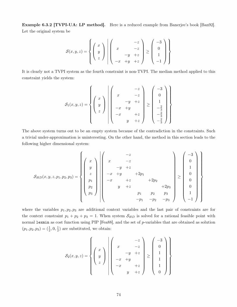
www.dedoimedo.com all rights reserved
Example 6.3.2 [TVPI-UA: LP method]. Here is a reduced example from Banerjee’s book [Ban92].Let the original system be
S(x, y, z) =
x
y
z
∣∣∣∣∣∣∣∣∣∣
−z
x −z−y +z
−x +y +z
≥−3
0
1
−1
It is clearly not a TVPI system as the fourth constraint is non-TVPI. The median method applied to thisconstraint yields the system:
S1(x, y, z) =
x
y
z
∣∣∣∣∣∣∣∣∣∣∣∣∣∣∣
−zx −z−y +z
−x +y
−x +z
y +z
≥
−3
0
1
−23
−23
−23
The above system turns out to be an empty system because of the contradiction in the constraints. Sucha trivial under-approximation is uninteresting. On the other hand, the method in this section leads to thefollowing higher dimensional system:
SHD(x, y, z, p1, p2, p3) =
x
y
z
p1
p2
p3
∣∣∣∣∣∣∣∣∣∣∣∣∣∣∣∣∣∣∣∣
−zx −z−y +z
−x +y +2p1
−x +z +2p2
y +z +2p3
p1 p2 p3
−p1 −p2 −p3
≥
−3
0
1
0
0
0
1
−1
where the variables p1, p2, p3 are additional context variables and the last pair of constraints are forthe context constraint p1 + p2 + p3 = 1. When system SHD is solved for a rational feasible point withnormal lexmin as cost function using PIP [Fea88], and the set of p-variables that are obtained as solution(p1, p2, p3) = (12 , 0,
12) are substituted, we obtain:
S2(x, y, z) =
x
y
z
∣∣∣∣∣∣∣∣∣∣∣∣∣∣∣
−zx −z−y +z
−x +y
−x +z
y +z
≥
−3
0
1
1
1
0
74
www.dedoimedo.com all rights reserved
The reader can verify the non-satisfiability of approximation S1 and satisfiability of the approximation S2.�
The above method involves only one call to a standard LP solver. The disadvantage is that the systemSHD(x,p) has n+
(‖aj‖2
)= n+ ‖aj‖(‖aj‖ − 1)/2 ≈ O(n+ ‖aj‖2) dimensions, where ‖aj‖ is the number
of non-zero elements in the vector aj . As the method involves a call to an LP solver, its theoretical costis not strongly polynomial time.
6.4 Multiple-constraint LP formulations
When there exist multiple non-TVPI constraints in S(x), each one of them has to be approximated tofind a TVPI approximation of the polyhedron. Let mk be the number of non-TVPI constraints in S(x),with mk ≤ m. Without loss of generality, we can assume that the constraints have been ordered such thatthe non-TVPI constraints come first, followed by the TVPI constraints. This means that the constraintsof S(x) are {1, . . . ,mk, . . . ,m}, with the constraints {1, . . . ,mk} being non-TVPI constraints and theconstraints {mk + 1, . . . ,m} being TVPI constraints.
6.4.1 One-shot method
A straightforward way in which one can find a TVPI approximation of the above non-TVPI system S(x) isto construct a system SHD(x,p1, . . . ,pmk) in which all the non-TVPI constraints in S(x) are approximatedusing the scheme described in Section 6.3.2. This system can be solved using an LP formulation in variablesas {x,p1, . . . , ,pmk}. An approximation of S(x) could be found as SHD(x,p1, . . . ,pmk)|p1, . . . ,pmk . Itcan easily be shown that the latter system is a proper approximation as long as the context constraints∑
p1 = b1, . . . ,∑
pmk = bmk are respected.
But, finding the approximations of all the non-TVPI constraints simultaneously in the above fashionwould lead to an LP system, with too an high increase in the number of dimensions. SHD(x,p1, . . . ,pmk)
could have up to
n+
mk∑l=1
(‖al‖2
)= n+
mk∑l=1
‖al‖(‖al‖ − 1)/2
dimensions which could be as large21 as O(n+ ‖Smk‖3), with ‖Smk‖ being the average number of non-zerocoefficients/elements in the non-TVPI constraints in S(x).
21Though ‖Smk‖ itself is a small number, there are cases even in PolyBench 2.0—like adi and fdtd-2d—for which, the
additional dimensional-increase by ‖Smk‖3 could be considerable. More importantly, the system is very skewed : with respect
to the ratio of constraints to variables, with respect to the presence of zero and non-zero elements in the constraint elements,as well as with respect to the number of equalities (leading to a non-trivial lineality space with high dimensions). For suchskewed systems, simplex based solvers like PIP take longer times, than the near cubic-time (of Observation 3.3.1 on page 28)that is generally observed. We are grateful to Paul Feautrier for pointing this complexity aspect of Simplex and PIP in apersonal communication.
75
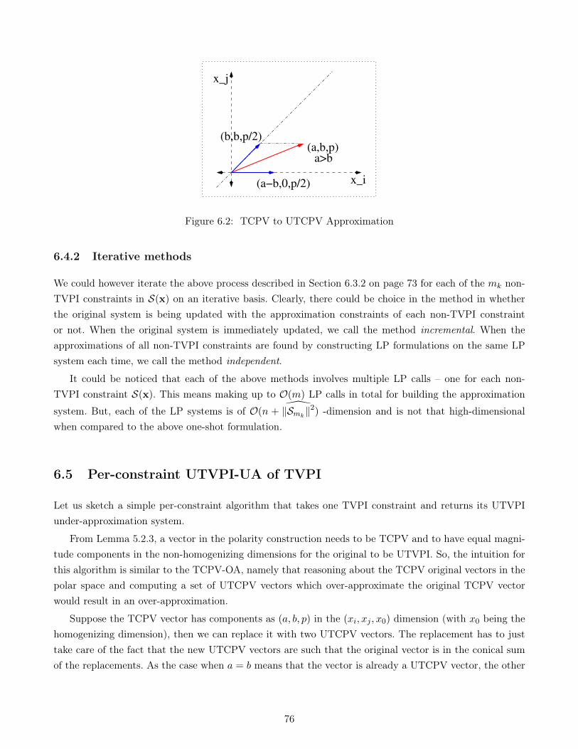
www.dedoimedo.com all rights reserved
(a,b,p)
x_i
x_j
(b,b,p/2)
(a−b,0,p/2)
a>b
Figure 6.2: TCPV to UTCPV Approximation
6.4.2 Iterative methods
We could however iterate the above process described in Section 6.3.2 on page 73 for each of the mk non-TVPI constraints in S(x) on an iterative basis. Clearly, there could be choice in the method in whetherthe original system is being updated with the approximation constraints of each non-TVPI constraintor not. When the original system is immediately updated, we call the method incremental. When theapproximations of all non-TVPI constraints are found by constructing LP formulations on the same LPsystem each time, we call the method independent.
It could be noticed that each of the above methods involves multiple LP calls – one for each non-TVPI constraint S(x). This means making up to O(m) LP calls in total for building the approximation
system. But, each of the LP systems is of O(n + ‖Smk‖2) -dimension and is not that high-dimensionalwhen compared to the above one-shot formulation.
6.5 Per-constraint UTVPI-UA of TVPI
Let us sketch a simple per-constraint algorithm that takes one TVPI constraint and returns its UTVPIunder-approximation system.
From Lemma 5.2.3, a vector in the polarity construction needs to be TCPV and to have equal magni-tude components in the non-homogenizing dimensions for the original to be UTVPI. So, the intuition forthis algorithm is similar to the TCPV-OA, namely that reasoning about the TCPV original vectors in thepolar space and computing a set of UTCPV vectors which over-approximate the original TCPV vectorwould result in an over-approximation.
Suppose the TCPV vector has components as (a, b, p) in the (xi, xj , x0) dimension (with x0 being thehomogenizing dimension), then we can replace it with two UTCPV vectors. The replacement has to justtake care of the fact that the new UTCPV vectors are such that the original vector is in the conical sumof the replacements. As the case when a = b means that the vector is already a UTCPV vector, the other
76
www.dedoimedo.com all rights reserved
cases can be handled in the following way:
a
b
p
∈
a > b : cone
b a− bb 0
p2
p2
a < b : cone
a 0
a b− ap2
p2
In either of the above cases, it can be noticed that the first vector is a UTCPV vector and the second isan interval vector. The first case is illustrated in Figure 6.2.
Lemma 6.5 [Validity of the above UTVPI approximation]. Given a TVPI constraint, the abovemethod returns a valid UTVPI-UA of the constraint.
Proof: The geometric proof derives from the observation that the sum of the corresponding UTCPVreplacement vectors is the original vector. Hence every vector in the polar space that is reachable by theoriginal vector is reachable by these replacement vectors, meaning that they give an OA in the polar space.In the primal space, the replacements necessarily give an UA (Cor. 5.3.1b). �
Example 6.5 [TVPI to UTVPI-UA]. Let PV = conv
{(1
1
),
(4
1
),
(1
2
)}, with the H-form
of P beingPH = {1 ≤ x ≤ 4; 1 ≤ y ≤ 2;x+ 3y ≤ 7}
It can be seen that P is trivially a TVPI system, but not a UTVPI system, as the third constraintx + 3y ≤ 7 is a non-UTVPI constraint. The UTVPI approximation by the above method is UA(PV) =
{1 ≤ x ≤ 4; 1 ≤ y ≤ 2;x+ y ≤ 72 ; 2y ≤ 7
2} which can be seen to be non-empty with vertices
UA(PV) = conv
{(1
1
),
(174
),
(52
1
),
(7474
)}
The under-approximation is shown in Figure 6.3. �
The cost of finding the UA is linear and the method is simple to implement, just like the medianmethod mentioned in Section 6.2. Just like that method, this method is not guaranteed to generate anon-empty under-approximated system.
77
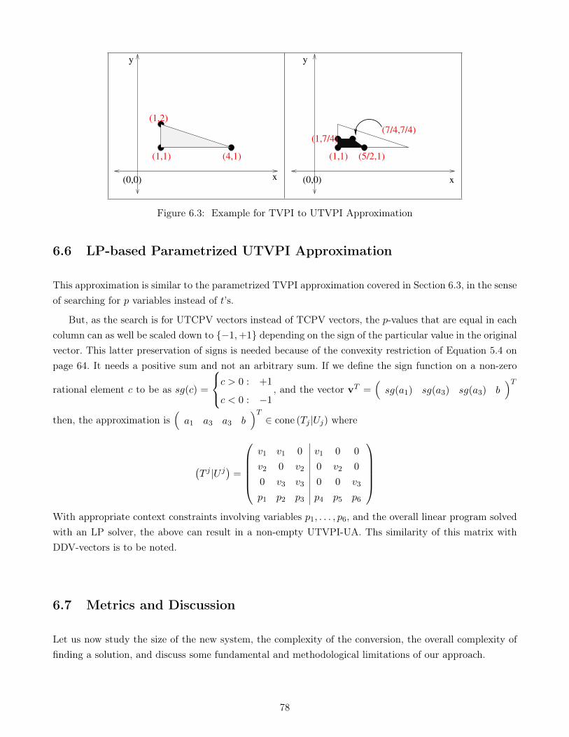
www.dedoimedo.com all rights reserved
y
x
(1,2)
(1,1) (4,1)
(0,0) x
y
(1,7/4)(7/4,7/4)
(0,0)
(1,1) (5/2,1)
Figure 6.3: Example for TVPI to UTVPI Approximation
6.6 LP-based Parametrized UTVPI Approximation
This approximation is similar to the parametrized TVPI approximation covered in Section 6.3, in the senseof searching for p variables instead of t’s.
But, as the search is for UTCPV vectors instead of TCPV vectors, the p-values that are equal in eachcolumn can as well be scaled down to {−1,+1} depending on the sign of the particular value in the originalvector. This latter preservation of signs is needed because of the convexity restriction of Equation 5.4 onpage 64. It needs a positive sum and not an arbitrary sum. If we define the sign function on a non-zero
rational element c to be as sg(c) =
c > 0 : +1
c < 0 : −1, and the vector vT =
(sg(a1) sg(a3) sg(a3) b
)Tthen, the approximation is
(a1 a3 a3 b
)T∈ cone (Tj |Uj) where
(T j |U j
)=
v1 v1 0 v1 0 0
v2 0 v2 0 v2 0
0 v3 v3 0 0 v3
p1 p2 p3 p4 p5 p6
With appropriate context constraints involving variables p1, . . . , p6, and the overall linear program solvedwith an LP solver, the above can result in a non-empty UTVPI-UA. Ths similarity of this matrix withDDV-vectors is to be noted.
6.7 Metrics and Discussion
Let us now study the size of the new system, the complexity of the conversion, the overall complexity offinding a solution, and discuss some fundamental and methodological limitations of our approach.
78
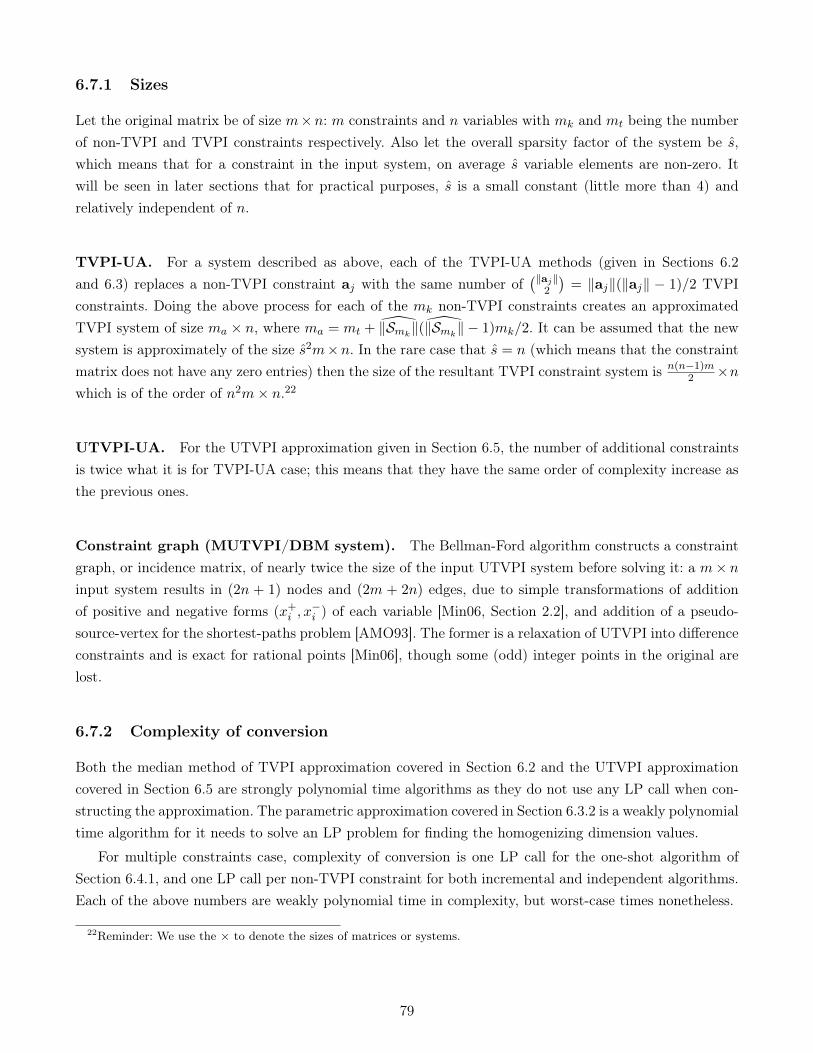
www.dedoimedo.com all rights reserved
6.7.1 Sizes
Let the original matrix be of size m×n: m constraints and n variables with mk and mt being the numberof non-TVPI and TVPI constraints respectively. Also let the overall sparsity factor of the system be s,which means that for a constraint in the input system, on average s variable elements are non-zero. Itwill be seen in later sections that for practical purposes, s is a small constant (little more than 4) andrelatively independent of n.
TVPI-UA. For a system described as above, each of the TVPI-UA methods (given in Sections 6.2and 6.3) replaces a non-TVPI constraint aj with the same number of
(‖aj‖2
)= ‖aj‖(‖aj‖ − 1)/2 TVPI
constraints. Doing the above process for each of the mk non-TVPI constraints creates an approximatedTVPI system of size ma × n, where ma = mt + ‖Smk‖(‖Smk‖ − 1)mk/2. It can be assumed that the newsystem is approximately of the size s2m×n. In the rare case that s = n (which means that the constraintmatrix does not have any zero entries) then the size of the resultant TVPI constraint system is n(n−1)m
2 ×nwhich is of the order of n2m× n.22
UTVPI-UA. For the UTVPI approximation given in Section 6.5, the number of additional constraintsis twice what it is for TVPI-UA case; this means that they have the same order of complexity increase asthe previous ones.
Constraint graph (MUTVPI/DBM system). The Bellman-Ford algorithm constructs a constraintgraph, or incidence matrix, of nearly twice the size of the input UTVPI system before solving it: a m× ninput system results in (2n + 1) nodes and (2m + 2n) edges, due to simple transformations of additionof positive and negative forms (x+i , x
−i ) of each variable [Min06, Section 2.2], and addition of a pseudo-
source-vertex for the shortest-paths problem [AMO93]. The former is a relaxation of UTVPI into differenceconstraints and is exact for rational points [Min06], though some (odd) integer points in the original arelost.
6.7.2 Complexity of conversion
Both the median method of TVPI approximation covered in Section 6.2 and the UTVPI approximationcovered in Section 6.5 are strongly polynomial time algorithms as they do not use any LP call when con-structing the approximation. The parametric approximation covered in Section 6.3.2 is a weakly polynomialtime algorithm for it needs to solve an LP problem for finding the homogenizing dimension values.
For multiple constraints case, complexity of conversion is one LP call for the one-shot algorithm ofSection 6.4.1, and one LP call per non-TVPI constraint for both incremental and independent algorithms.Each of the above numbers are weakly polynomial time in complexity, but worst-case times nonetheless.
22Reminder: We use the × to denote the sizes of matrices or systems.
79

www.dedoimedo.com all rights reserved
6.7.3 Complexity of finding a feasible solution
For the TVPI approximation, as the worst-case complexity of Hochbaum-Naor is O(mn2 logm) [HN94],applying it to the resultant approximated system would lead to O(s2mn2 log sm) time with constraintsparsity s, and O(n4m log nm) in the unlikely case when s = O(n).
For the UTVPI approximation, as the theoretical worst-case complexity of solving UTVPI systems isO(mn) (if we use the traditional Bellman-Ford algorithm on the difference constraints), the correspond-ing complexities would be O(s2mn), and O(n3m) respectively. In Chapter 7, we see empirical evidencesuggesting that in practise, a TVPI constraint always turns out to be a UTVPI constraint, making thismethod very attractive.
6.7.4 Preprocessing and Limitations
It can be noticed that our algorithms do not ask for removal of redundant inequalities, which is as hardas determining if the input system is feasible.
Polyhedra in compilation have lot of duplicate constraints, which gets reflected in the approximations aswell. Compilers like PLuTo remove these by methods like textual matching which leads to a large decreasein the number of constraints. A more advanced scheme, finely-tuned to UTVPI constraints, would use ahashing or radix-sort technique [AN98] packing the UTVPI constraint in a few integers: exploiting the factthat the non-homogenizing dimension values are from {0,±1}, while the homogenizing dimension valuesare always from a very small set [−5, 5]. It would bring the simplification complexity to linear time. Wethus believe that the problem of duplicate elimination is asymptotically insignificant or can be dividedper-dependence-edge as amortized-cost in addition to other fixed costs like dependence feasibility tests,Farkas multiplier simplification and Gaussian eliminations.
The following example shows an inherent limitation of the process of TVPI-UA itself.
Example 6.7.4 [Polyhedra with non-satisfactory approximations]. The polyhedron describedusing the constraints {x + y + z ≥ −1; x + y + z ≤ 1} is not TVPI. Though it is unbounded in bothdirections, the only TVPI approximations that are possible of the above polyhedron are bounded TVPIpolyhedra, which can be considered a failure of the UA approach. Similarly, the TVPI polyhedron (whichis non-UTVPI) described by the constraints {x+ 2y ≥ −1; x+ 2y ≤ 1} can only be under-approximatedby UTVPI polyhedra that are finite. The second (planar) example is shown in Figure 6.4. �
The above kinds of polyhedra can be considered as degenerate cases and identified by a pre-processingstep that removes the lineality space from the input polyhedron. Furthermore, the Farkas polyhedra thatarise in polyhedral scheduling are always pointed polyhedra and can never have non-trivial lineality space.
6.7.5 Integer scaling and TU polyhedra
One limitation of the parametric approximations of Sections 6.3 and 6.6 is that they may result in rationalpolyhedra, whose constraints are of the form axi+bxj ≤ c; a, b, c ∈ Q for TVPI and ±xi±xj ≤ c; c ∈ Q, forUTVPI. Having such rational polyhedron as approximations could be a limitation in cases when an integer
80
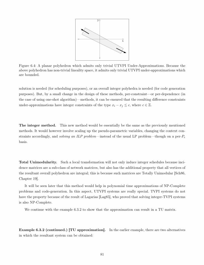
www.dedoimedo.com all rights reserved
y
x
Figure 6.4: A planar polyhedron which admits only trivial UTVPI Under-Approximations. Because theabove polyhedron has non-trivial lineality space, it admits only trivial UTVPI under-approximations whichare bounded.
solution is needed (for scheduling purposes), or an overall integer polyhedra is needed (for code generationpurposes). But, by a small change in the design of these methods, per-constraint—or per-dependence (inthe case of using one-shot algorithm)—methods, it can be ensured that the resulting difference constraintsunder-approximations have integer constraints of the type xi − xj ≤ c, where c ∈ Z.
The integer method. This new method would be essentially be the same as the previously mentionedmethods. It would however involve scaling up the pseudo-parametric variables, changing the context con-straints accordingly, and solving an ILP problem—instead of the usual LP problem—though on a per-Pebasis.
Total Unimodularity. Such a local transformation will not only induce integer schedules because inci-dence matrices are a sub-class of network matrices, but also has the additional property that all vertices ofthe resultant overall polyhedron are integral; this is because such matrices are Totally Unimodular [Sch86,Chapter 19].
It will be seen later that this method would help in polynomial time approximations of NP-Completeproblems and code-generation. In this aspect, UTVPI systems are really special. TVPI systems do nothave the property because of the result of Lagarias [Lag85], who proved that solving integer-TVPI systemsis also NP-Complete.
We continue with the example 6.3.2 to show that the approximation can result in a TU matrix.
Example 6.3.2 (continued.) [TU approximation]. In the earlier example, there are two alternativesin which the resultant system can be obtained:
81
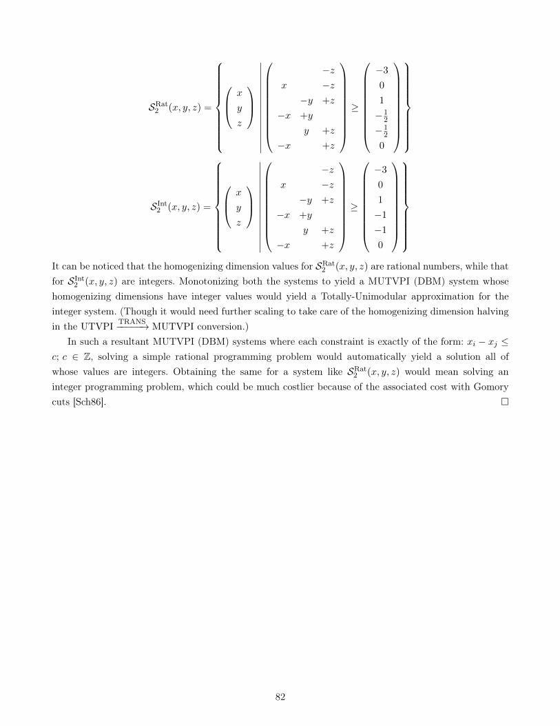
www.dedoimedo.com all rights reserved
SRat2 (x, y, z) =
x
y
z
∣∣∣∣∣∣∣∣∣∣∣∣∣∣∣
−zx −z−y +z
−x +y
y +z
−x +z
≥
−3
0
1
−12
−12
0
SInt2 (x, y, z) =
x
y
z
∣∣∣∣∣∣∣∣∣∣∣∣∣∣∣
−zx −z−y +z
−x +y
y +z
−x +z
≥
−3
0
1
−1
−1
0
It can be noticed that the homogenizing dimension values for SRat
2 (x, y, z) are rational numbers, while thatfor SInt2 (x, y, z) are integers. Monotonizing both the systems to yield a MUTVPI (DBM) system whosehomogenizing dimensions have integer values would yield a Totally-Unimodular approximation for theinteger system. (Though it would need further scaling to take care of the homogenizing dimension halvingin the UTVPI
TRANS−−−−−→ MUTVPI conversion.)In such a resultant MUTVPI (DBM) systems where each constraint is exactly of the form: xi − xj ≤
c; c ∈ Z, solving a simple rational programming problem would automatically yield a solution all ofwhose values are integers. Obtaining the same for a system like SRat
2 (x, y, z) would mean solving aninteger programming problem, which could be much costlier because of the associated cost with Gomorycuts [Sch86]. �
82

www.dedoimedo.com all rights reserved
6.8 Conclusions and Perspectives
In this section, we first discuss some conclusions and contributions, and then present some perspectives.
6.8.1 Conclusions and contributions
In this chapter, we began with the framework given in the previous chapter and gave under-approximationalgorithms that take a general convex polyhedron and give some (U)TVPI under-approximations. Thealgorithms take polynomial time. The Table 6.1 summarizes the complexities of the methods introducedin this chapter:
Conversion of Polyhedra(UA/TRANS)
MetricSizes Complexity of
Conversion(LP basedmethods)
Improvementin Complexityof Solution
PolyUA−−→ TVPI m× n UA−−→
s2m× nZ(s2m,n) Z(m,n) to
O(s2mn2 log sm)
TVPIUA−−→ UTVPI m× n UA−−→
2m× nZ(m,n) O(mn2 logm)
to O(mn)
UTVPITRANS−−−−−→ MUTVPI m× n TRANS−−−−−→
(2m+ 2n)×(2n+ 1)incidencematrix
– O(mn) toO(mn) (No lossof precision inrational case.)
PolyUA−−→ MUTVPI m× n UA−−→
(O(s2m+2n))× (2n+ 1)
TableauUA−−→
Incidence matrix
Z(s2m,n) Z(m,n) toO(s2mn)
Table 6.1: Complexities of Under-Approximation Algorithms
Contributions. The problem of finding an (U)TVPI-UA of a convex polyhedron is both easy anddifficult because there are many solutions to the problem; for a given convex polyhedron, there alwaysexists a non-empty (U)TVPI under-approximation. We have defined algorithms that are simple, run inpolynomial time employing linear programming, and are easy to illustrate in an algorithmic and geometricsense. We believe that these algorithms can be used as they are, or can be used as a framework to designother (U)TVPI-UA algorithms.
In Section 6.7.5 we introduced an algorithm which involves solving an ILP problem on a per-dependencebasis, with the result that the overall polyhedron has integral (not just rational) properties. We also believethat this is a unique contribution to polyhedral compilation, because it helps the overall intersection ofper-dependence polyhedra to very cheaply have integer vertices. The system obtained can be solved using
83

www.dedoimedo.com all rights reserved
Bellman-Ford with a very low polynomial time cost. This is because the per-dependence edge polyhedra aremostly trivially small and solving ILP problem on them is usually never more costly than solving a normalLP problem. As far as we know, this method has not been previously explored in polyhedral compilationup to now. In Chapter 8 on page 101 we study some potential applications of this method. In this aspect,it should be noted that UTVPI polyhedra are special, even when compared to TVPI polyhedra. becauseof the result of Lagarias [Lag85] who proved the NP-Completeness of solving integral TVPI-systems, sucha Totally Unimodular approximation is not possible even with TVPI polyhedra.
6.8.2 Perspectives and discussion
Different methods for using the UA algorithms. For converting an arbitrary convex polyhedroninto a TVPI under-approximating polyhedron so that Hochbaum-Naor’s algorithm [HN94] can be used,the method is the following: Poly
UA−−→ TVPI. On the other hand, for converting into a UTVPI polyhedronso that Bellman-Ford algorithm can be used to solve the resultant, the method we suggest is the following:
PolyUA−−→ TVPI
UA−−→ UTVPITRANS−−−−−→ MUTVPI (6.2)
For this latter process, one can alternatively choose the method PolyUA−−→ UTVPI
TRANS−−−−−→ MUTVPI,where the intermediate step of involving TVPI polyhedra is skipped, but there is seldom any loss ofprecision when doing the approximation TVPI
UA−−→ UTVPI. This is due to the nature of constraints inpolyhedral compilation, which already have TVPI-ness and constraints that are already TVPI are highlylikely to be UTVPI as well. Direct UTVPI approximation from Poly to UTVPI would mean insertion of6 vectors: the normal 3 UTCPV vectors and an additional 3 interval vectors corresponding to interval
constraints: vectors of the form
±1
0
0
,
0
±1
0
and
0
0
±1
, where the sign of the ±1 vector is
determined by the sign of the particular component of the vector that it is approximating.
Feasibility control. One important characteristic of under-approximation methods is the preservationor not of the feasibility of the UA. In this respect, the median method though having other advantages–like for example, ease of implementation–comes with the serious weakness that it offers no guaranteeof preservation of feasibility when the input polyhedron is non-empty. The LP-independent method andLP-incremental methods are a little better in this respect, and only the one-shot method comes with anabsolute guarantee that the UA is always non-empty when the input is. This aspect will be covered morein Chapters 7 and 8, where more advanced clustering techniques are discussed and implemented so thatthe output, in the presence of intersection of many polyhedra can come with such a guarantee. The overallintersection of under-approximations is ensured to be non-empty.
Necessity of polarity framework. The previous chapter discussed two alternate ways of reasoningabout the approximations: a homogenization-polarity framework along with the equivalent applicationof affine form of Farkas lemma. One question this raises is whether the former is really needed. One
84

www.dedoimedo.com all rights reserved
traditional answer is that the homogenization-polarity framework is completely subsumed by the Farkaslemma application and hence the former is redundant. But, it is our opinion that the use of polarity (inparticular conical polarity) is a unique contribution to this aspect. It is indeed true that Farkas lemmamakes the former redundant, but, it is also true that with Farkas lemma being such a fundamental aspectof analysis of convex polyhedra, everything else in it comes literally for free once it is assumed.
Also, the duality concept and Farkas lemma are exactly equivalent to each other, both having theirground in Farkas-Minkowski-Weyl theorem about finite generation of convex cones [Sch86, Cor. 7.1a]. So,the criticism that the polarity framework is redundant because it uses duality stands on weak ground.The reconciliation could be that the polarity framework uses the geometric aspect of duality, while theequivalent Farkas lemma application uses the equational aspect of duality.
The polarity framework offers a couple of adantages as well. Primarily, the construction using polarityoffers a unique geometric perspective finding approximations. This latter aspect is obviously not providedby the Farkas lemma application. Also, the polarity construction can obviously be extended for the dualproblem of OA as well. Furthermore, when applied to the problem of finding (U)TVPI-UA of a generalconvex polyhedron, it offers many choices, mainly because there are many ways of choosing a valid UA.Other users of the approximation framework, like for solving verification problems, may find that the studyof the framework while designing their UAs be useful to provide hints at the kind of approximation thatwould suit their purposes.
More powerful alternatives
Other than the LP based methods that we proposed to find (U)TVPI-UA of a polyhedron, we study twoalternative methods to do the same and show their limitations: one using generator representation andanother using non-linear solvers or quantifier elimination methods. Obviously, neither of them scale on theoverall P and the only scalable means of running them would be on a per-Pe basis.
Generator representation. The straightforward alternative of finding UA is to use the generatorrepresentation of the (U)TVPI polyhedra. This algorithm could be similar to the OA algorithm designedby Miné for UTVPI polyhedra and studied in Section 4.3.2 on page 50. Such a method could have aguarantee of non-emptiness of the approximation, and as well as an additional guarantee with respect tothe volume ratio of with respect to the original. The LP based method provides the former in its one-shot variation, but not the latter. Obviously, this method comes with the prohibitive exponential costassociated with Chernikova algorithm. Except for some benchmarks—like pca and tce—in PolyBench 3.0,such a method may be acceptable on a per-dependence basis. But, the advantages it comes with are onlyon a single polyhedron case. Since the problem in polyhedral compilation involves intersections of manyper-dependence polyhedra, such prohibitive asymptotic cost may not tolerable, except in some offline andonline compilation methods.23
23The biggest open problem here is of course to study if Under/Over-Approximation of convex polyhedra using UTVPIpolyhedra may help in obtaining a strongly polynomial time bounds for the optimization problem for convex problem, asshown in Figure 6.5.
85
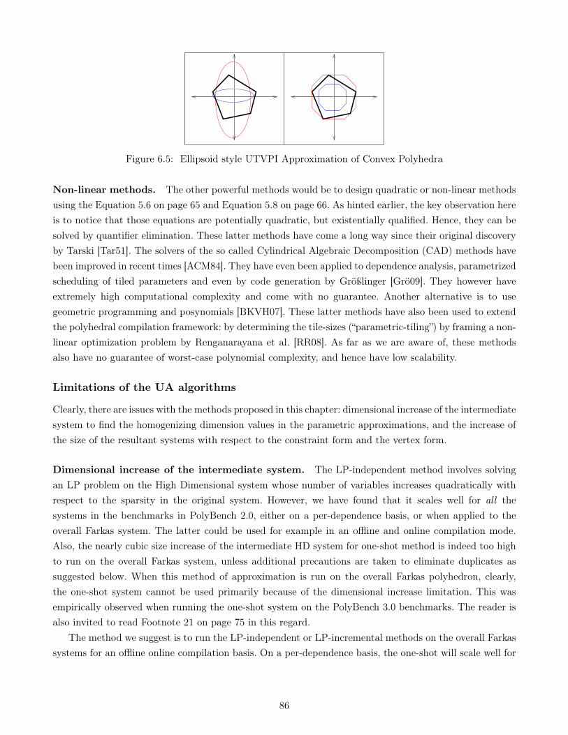
www.dedoimedo.com all rights reserved
Figure 6.5: Ellipsoid style UTVPI Approximation of Convex Polyhedra
Non-linear methods. The other powerful methods would be to design quadratic or non-linear methodsusing the Equation 5.6 on page 65 and Equation 5.8 on page 66. As hinted earlier, the key observation hereis to notice that those equations are potentially quadratic, but existentially qualified. Hence, they can besolved by quantifier elimination. These latter methods have come a long way since their original discoveryby Tarski [Tar51]. The solvers of the so called Cylindrical Algebraic Decomposition (CAD) methods havebeen improved in recent times [ACM84]. They have even been applied to dependence analysis, parametrizedscheduling of tiled parameters and even by code generation by Größlinger [Grö09]. They however haveextremely high computational complexity and come with no guarantee. Another alternative is to usegeometric programming and posynomials [BKVH07]. These latter methods have also been used to extendthe polyhedral compilation framework: by determining the tile-sizes (“parametric-tiling”) by framing a non-linear optimization problem by Renganarayana et al. [RR08]. As far as we are aware of, these methodsalso have no guarantee of worst-case polynomial complexity, and hence have low scalability.
Limitations of the UA algorithms
Clearly, there are issues with the methods proposed in this chapter: dimensional increase of the intermediatesystem to find the homogenizing dimension values in the parametric approximations, and the increase ofthe size of the resultant systems with respect to the constraint form and the vertex form.
Dimensional increase of the intermediate system. The LP-independent method involves solvingan LP problem on the High Dimensional system whose number of variables increases quadratically withrespect to the sparsity in the original system. However, we have found that it scales well for all thesystems in the benchmarks in PolyBench 2.0, either on a per-dependence basis, or when applied to theoverall Farkas system. The latter could be used for example in an offline and online compilation mode.Also, the nearly cubic size increase of the intermediate HD system for one-shot method is indeed too highto run on the overall Farkas system, unless additional precautions are taken to eliminate duplicates assuggested below. When this method of approximation is run on the overall Farkas polyhedron, clearly,the one-shot system cannot be used primarily because of the dimensional increase limitation. This wasempirically observed when running the one-shot system on the PolyBench 3.0 benchmarks. The reader isalso invited to read Footnote 21 on page 75 in this regard.
The method we suggest is to run the LP-independent or LP-incremental methods on the overall Farkassystems for an offline online compilation basis. On a per-dependence basis, the one-shot will scale well for
86
www.dedoimedo.com all rights reserved
most of the benchmarks in polyhedral compilation. For the rest of the cases it may be necessary to runthe LP-independent or LP-incremental method on the per-dependence edge systems, but in those veryrare cases, we suggest using the LP-independent method because of the simplicity of the approach, andthe ease of implementation.
We see in Chapter 7 that the LP-Independent method is quite scalable. We have also found fromexperiments that the one-shot algorithm on the per-dependence edge basis is scalable as well, because thenumber of non-TVPI constraints on a per-Pe basis is quite low.
So as to limit the dimensional increase, additional precautions, like temporary removal of the zerodimensions in the HD system, one in which all the variables do not have any active components, couldbe done. Though we have not implemented this method, it is likely to help in the scaling of any of themethods and especially on a per-dependence edge basis, where many variables are likely to be inactive.
Increase in number of constraints (and generators). A quadratic increase in the number of resul-tant constraints proportional to sparsity (s2) for each of the methods suggested in this chapter may seemexcessive. But, it seems unavoidable because of the topological nature (limitedness) of TVPI constraintswhen compared to general convex polyhedra. It is also a matter of fact that the resultant systems havean increase in the number of vertices. If the resultant of these UA algorithms are converted to a generatorrepresentation, for instance for verification purposes, then, a heuristic bounding of these could be applied.See for example Kanade et al. [KAI+09].
Duplicate constraints. Related to the above is the increase in the duplicates in the resultant over-approximated systems. As suggested in Section 6.7.4, they can removed by a post-processing step exploitingthe simple nature of the output (U)TVPI-UA systems. But, the duplicates can also be limited before theLP call itself, by taking into account the repetition among the pairs of coefficients. For example, whenconstructing the TVPI-UA of the system {2x+ 3y+ 4z ≤ 1; 2x+ 3y− 4z ≤ 1} by using one-shot method,the normal method is to construct the HD system independent of the fact that the coefficients of x andy variable pair in the two constraints are exactly the same. Instead, the HD system could be formulatedtaking this fact into account: having fewer variables and constraints in the HD system. Though thisleads to the formulation where the pseudo-parametric constraints have to be formulated carefully, such animprovement also leads to having fewer constraints in the resultant UA system.
More details that are discussed at the end of next chapter, where the results of implementation of thesealgorithms in the PLuTo source-to-source compiler will be presented.
87

www.dedoimedo.com all rights reserved
88
Chapter 7
Experimental Evaluation ofUnder-Approximations
In this chapter, we study the experimental results of the UA-algorithms designed in the previous chapter.
7.1 Introduction
We carried out systematic experiments, tiling and parallelizing the 16 PolyBench (2.0) [PB+] benchmarksshipped along with the source-to-source polyhedral optimizer PLuTo (PLuTo-0.6). After our experiments,a new version PLuTo (PLuTo-0.8) was released and which optionally uses ISL instead of PIP. Farkassystems are extracted from PLuTo. We compare the default linear programming calls to PIP [Fea88] withthe TVPI-UA and then the UTVPI-UA algorithms. The UTVPI-UA is further relaxed into a constraintgraph (or incidence matrix) which is fed to our implementation of the Bellman-Ford algorithm, along withthe supporting routines. This process is:
PolyUA−−→ TVPI
UA−−→ UTVPITRANS−−−−−→ MUTVPI
BellmanFord−−−−−−−−→
Our experimental framework used the PiPLib [Fea88] and PolyLib [Wil93] libraries, with an option touse FMLib [Pou] as well. Note that we still use PIP for the much smaller linear programming problemsarising from the feasibility enhancing heuristics. Also, PLuTo makes use of PIP in parts unrelated withthe scalability of affine scheduling problems: the PIP calls from PLuTo originate from the functions:dep_satisfaction_test (DS), get_dep_direction (DIR) and find_permutable_hyperplanes (FPH).
We focus on FPH calls which correspond to affine scheduling problems. There are many more callsof the DS and DIR varieties, more than two orders of magnitude, when compared to the FPH calls, butthe optimization of the former pair of LP calls is entirely a different problem from the FPH variety inmany ways. Primarily, the former are dependence polyhedra and need to be over-approximated [DRV00,UC11] (Section 4.1.1 on page 37) as otherwise, incorrect transformations would result. The latter of courseare Farkas polyhedra, the main topic of this experimentation following our new scheme in Chapter 4(Section 4.4 on page 52), and need to be under-approximated leading to a conservative approximation and
89
www.dedoimedo.com all rights reserved
perhaps a loss of useful schedules.
7.2 Features of the polyhedra
Here we are referring to Table 7.1. The initial three columns refer to the size of the loop nest: L is thenumber of loops, S the number of statements, and D the number of dependences. The next sets of columnsindicate the polyhedral characteristics for the different varieties of calls in PLuTo. As the DS and DIRvariety are similar types of calls, they have been summarized together.
The number of polyhedra of different types are indicated in the P columns (PDS, PDIR and PFPH). Aswritten earlier, there are lot more polyhedral calls of DS/DIR than FPH. But, assuming that the loop-nestdepth d is a small bounded constant, the former are smaller systems and are linearly dependent on thesize of the loop nest: O(max(|E|, |V |). For a particular benchmark and variety of polyhedra (DS/DIRor FPH), n and m columns indicate the number of variables (unknowns), and the average number ofconstraints in the particular LP formulation respectively. The mt column indicates the average number ofTVPI constraints for that benchmark and variety of call.
DS/DIR. As it can be expected, most of the constraints in the DS/DIR polyhedra are TVPI constraints.In these polyhedra, there is never more than 1 constraint per polyhedron which is non-TVPI. In all thecases, whenever a constraint is TVPI, it is always turns out to be a UTVPI constraint, having the sameabsolute magnitude for the two coefficients, when it has two entries. An interval constraint like xi ≤ c orxi ≥ c, with only one non-zero coefficient, is of course UTVPI as well.
FPH. In the FPH variety, it can be noticed that the sizes of some of the FPH polyhedra are smalland comparable to the DS/DIR polyhedra. This is either the result of a small problem size or becausePLuTo uses Gaussian and Fourier-Motzkin elimination, along with a syntactic heuristic to reduce theduplicate constraints. As it can be expected, mt, number of TVPI constraints in the original system, ishighly benchmark dependent. But, just like in DS/DIR polyhedra, a TVPI constraint always happens tobe a UTVPI constraint.‖Smk‖ is the average number of non-zero coefficients in the non-TVPI constraints for that benchmark.
It can be seen that this number, though again being benchmark dependent, is a small constant whencompared to the dimension size n. ma is the number of constraints in the new (approximated TVPI)system. As seen earlier, ma = ‖Smk‖(‖Smk‖ − 1)(m−mt)/2 +mt.
The relative growth of the approximated system with respect to the original one is defined as the ratiobetween the sum of entries in the ma and m columns. We found the average value of this to be 8, meaningthat the overall sparsity factor s is a little more than 4. Sometimes the growth of the approximated systemis significant, but it has to be remembered that ma is the number of constraints without any simplification,while m is the obtained after systematic simplification and elimination of duplicates in PLuTo.
For comparison purposes with ma, we have added the mu column, which is the average unsimplifiedsystem size when the simplification techniques used in PLuTo are turned off. It can be observed thatmu and ma are comparable. Across all benchmarks, our experience shows that the approximated system
90
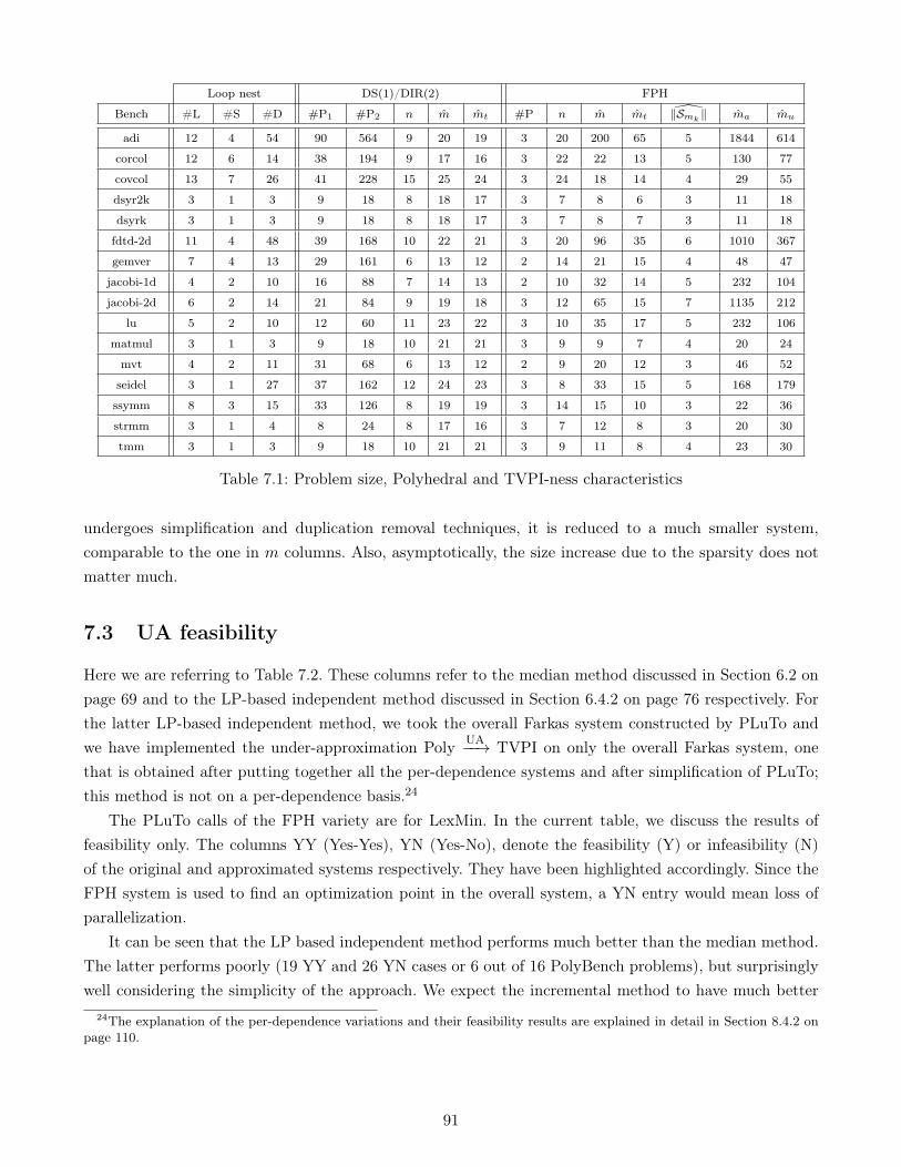
www.dedoimedo.com all rights reserved
Loop nest DS(1)/DIR(2) FPH
Bench #L #S #D #P1 #P2 n m mt #P n m mt ‖Smk‖ ma mu
adi 12 4 54 90 564 9 20 19 3 20 200 65 5 1844 614
corcol 12 6 14 38 194 9 17 16 3 22 22 13 5 130 77
covcol 13 7 26 41 228 15 25 24 3 24 18 14 4 29 55
dsyr2k 3 1 3 9 18 8 18 17 3 7 8 6 3 11 18
dsyrk 3 1 3 9 18 8 18 17 3 7 8 7 3 11 18
fdtd-2d 11 4 48 39 168 10 22 21 3 20 96 35 6 1010 367
gemver 7 4 13 29 161 6 13 12 2 14 21 15 4 48 47
jacobi-1d 4 2 10 16 88 7 14 13 2 10 32 14 5 232 104
jacobi-2d 6 2 14 21 84 9 19 18 3 12 65 15 7 1135 212
lu 5 2 10 12 60 11 23 22 3 10 35 17 5 232 106
matmul 3 1 3 9 18 10 21 21 3 9 9 7 4 20 24
mvt 4 2 11 31 68 6 13 12 2 9 20 12 3 46 52
seidel 3 1 27 37 162 12 24 23 3 8 33 15 5 168 179
ssymm 8 3 15 33 126 8 19 19 3 14 15 10 3 22 36
strmm 3 1 4 8 24 8 17 16 3 7 12 8 3 20 30
tmm 3 1 3 9 18 10 21 21 3 9 11 8 4 23 30
Table 7.1: Problem size, Polyhedral and TVPI-ness characteristics
undergoes simplification and duplication removal techniques, it is reduced to a much smaller system,comparable to the one in m columns. Also, asymptotically, the size increase due to the sparsity does notmatter much.
7.3 UA feasibility
Here we are referring to Table 7.2. These columns refer to the median method discussed in Section 6.2 onpage 69 and to the LP-based independent method discussed in Section 6.4.2 on page 76 respectively. Forthe latter LP-based independent method, we took the overall Farkas system constructed by PLuTo andwe have implemented the under-approximation Poly
UA−−→ TVPI on only the overall Farkas system, onethat is obtained after putting together all the per-dependence systems and after simplification of PLuTo;this method is not on a per-dependence basis.24
The PLuTo calls of the FPH variety are for LexMin. In the current table, we discuss the results offeasibility only. The columns YY (Yes-Yes), YN (Yes-No), denote the feasibility (Y) or infeasibility (N)of the original and approximated systems respectively. They have been highlighted accordingly. Since theFPH system is used to find an optimization point in the overall system, a YN entry would mean loss ofparallelization.
It can be seen that the LP based independent method performs much better than the median method.The latter performs poorly (19 YY and 26 YN cases or 6 out of 16 PolyBench problems), but surprisinglywell considering the simplicity of the approach. We expect the incremental method to have much better
24The explanation of the per-dependence variations and their feasibility results are explained in detail in Section 8.4.2 onpage 110.
91

www.dedoimedo.com all rights reserved
Median LP-IndepBench YY YN YY YN
adi 0 3 0 3
corcol 1 2 0 3
covcol 3 0 3 0
dsyr2k 3 0 3 0
dsyrk 3 0 3 0
fdtd-2d 0 3 1 2
gemver 0 2 2 0
jacobi-1d 0 2 0 2
jacobi-2d 0 3 0 3
lu 0 3 0 3
matmul 3 0 3 0
mvt 0 2 2 0
seidel 0 3 3 0
ssymm 3 0 3 0
strmm 0 3 3 0
tmm 3 0 3 0
Total 19 26 29 16
Table 7.2: UA effectiveness: Median and LP-Independent methods (PolyBench 2.0)
performance than the current independent method (29 YY and 16 YN cases or 10 out of 16 PolyBenchproblems).
7.4 Scalability comparison: Simplex vs. Bellman-Ford
Figures 7.1 and 7.2 show the execution times of the Simplex on the original system vs. Bellman-Ford (BF)on a UTVPI approximated system25.
• The former uses the quite well used dual-simplex implementation of PIP [Fea88] (similar [Tod02] tomany LP solvers like CPLEX [Bix02]) called on a (non-parametric) rational polyhedron for feasibility.
• The latter is our implementation of a standard Bellman-Ford algorithm on the constraint-graph ofalmost double size obtained from the MUTVPI-polyhedron (the monotonized-UTVPI polyhedron)called for testing the presence of negative weight cycles.
The input programs matmul and seidel are the same as in Figures 2.2 on page 12, and each call ofauto_trans of PLuTo to find schedule hyperplanes has tens of calls of the above variety, which explainsthe difference in scales between current figures (Figure 7.1 and 7.2) and in Figure 2.3 on page 13. Prior tosolving either of these, the duplicates were eliminated using a syntactic matching as in PLuTo. Even onthe systems with duplicates, the improvements were similar, though more prominent.
25The UTVPI system used in these scalability experiments is obtained as a result of a clustering algorithm. This particularalgorithm, called PD4, is a part of our methods to improve feasibility of the under-approximation. These are explained indetail in Section 8.4.2 on page 110
92

www.dedoimedo.com all rights reserved
0 1000 2000 3000 4000
01
23
Time taken to Solve System (Seconds) vs. Number of Dependences
Dependences
Tim
e taken (
Seconds)
Solve (SCoP)
PIP (MAT)BF (MAT)
Figure 7.1: Simplex (PIP) vs. Bellman-Ford (BF) for unrolled examples of matmul (ITR-MATMUL)
0 1000 2000 3000 4000 5000 6000
0.0
0.1
0.2
0.3
0.4
0.5
0.6
0.7
Time taken to Solve System (Seconds) vs. Number of Dependences
Dependences
Tim
e taken (
Seconds)
Solve (SCoP)
PIP (SEI)BF (SEI)
Figure 7.2: Simplex (PIP) vs. Bellman-Ford (BF) for unrolled example of seidel (ITR-SEIDEL)
93

www.dedoimedo.com all rights reserved
Perf. Comparison (Seconds)
Benchmark Orig Par cur Par new Til cur Til new
gemver 0.31 0.15 0.15 0.15 0.15
mvt 1.40 0.27 0.28 0.42 0.43
seidel 11.8 3.6 3.6 11.5 11.5
Table 7.3: UA Code Performance. The Orig column indicates the execution times of the particular un-optimized benchmark. Columns Par cur and Til cur respectively indicate the execution times of theparallelized and tiled programs obtained by running PLuTo on the benchmarks. Columns Par cur and Tilcur respectively indicate the execution times of the parallelized and the tiled programs when the overallFarkas system is replaced by the TVPI under-approximated system obtained as a result of running theLP-independent method.
It can be seen from the graphs that for their respective inputs, BF (worst-case O(s2mn) ≈ O(|E||V |) ≈O(|V |3)) is asymptotically as well as empirically faster than PIP’s Simplex (observed O((m + n)mn) ≈O(|V |5)) (not counting that it is weakly polynomial time), meeting the scalability challenge. The regressioncoefficients (linear R2 using the R statistical package [R]) for the above formulae are around 99.9%. Thecurves for BF appear linear because the x-axis counts the number of dependences |E|, which is practicallyO(|V |2). Though the memory improvements are not shown in the above graphs, the linear memory (worst-case O(m+n)) of BF is considerably lighter26 than the quadratic memory (worst-case O(mn)) of Simplex.
The relatively lesser magnitudes and hence lesser improvements of seidel when compared to matmul
could be attributed to the fact that while the former has just uniform dependences which are easilyamenable to the Gaussian eliminations of PIP, the latter has more affine dependences and also inducesmany more Farkas multiplier variables. From the magnitude of each of these curves and the relativeimprovements for these two example programs, it is safe to say that sub-polyhedral techniques wouldprovide more significant improvements for programs with predominant affine dependences than for oneswith predominant uniform dependences.
7.5 UA generated code performance
We are referring here to Table 7.3, limiting ourselves to a subset of the YY cases in the previous tablethat our current implementation could handle. In each case, we replaced the original system(s) by theapproximated TVPI ones obtained by the independent LP method. The cost function was unchangedand the solution was found using PIP. It can be seen that performance gains closely match the defaultpolyhedral method in PLuTo, despite the approximation taking place. The impact of YN approximationson PLuTo’s effectiveness is yet to be studied, but we express some hope on PLuTo’s loop distributionheuristic to break infeasible systems.
Though the experiments in Table 7.3 are limited in number, obtaining these itself involved a consid-erable engineering effort in a research prototype tool like PLuTo. This was partly because of our explicit
26Initial evaluation on a Quad-Core Dell desktop with 16GB memory using the top program of linux showed up to 40%memory occupied by PIP program for an ITR-MATMUL program of around 4000 dependences. The memory occupied by BFwas always less than 10%. Though more exhaustive experiments are needed, we believe that these differences are significant.
94

www.dedoimedo.com all rights reserved
decision to not invest much further on the experimental front. We also chose to defer further evaluationuntil PLuTo is adapted to facilitate the integration of per-dependence approximations, and some engi-neering issues with the interpretation of PIP results could be circumvented. Examples of these issuesinclude methods to interpret the schedules obtained by the Bellman-Ford algorithm to obtain permutablehyperplanes, and ways to integrate them with the rest of the scheduler, as well as need to reengineerPLuTo’s backend—for example in function like pluto_detect_transformation_properties—so that theper-dependence systems can be replaced by their under-approximated systems—perhaps obtained by theone-shot algorithm—in a streamlined fashion, along with calling the necessary routines like duplicate elim-ination and feasibility testers at proper check-point locations. More details on some of these are discussedin the perspectives section at the end of this chapter.
7.6 UA verification
We used PIP and PolyLib matrices which were compatible even with other libraries like FMLib. Thisopened up some possibilities of using available routines from any of these libraries for checking feasibilityof the systems. PolyLib has a routine, PolyhedronIncludes, that takes two Polyhedra P and Q andreturns whether P ⊆ Q. It needs P and Q in generator representation and checks for inclusivity of each ofthe vertices of P in Q. Obviously, such a method does not work the large schedule matrices that PLuTohandles.
Another option is to verify the under-approximation using PIP while both P andQ are still in constraintform. This would involve framing an LP call to verify that none of negations of each of the constraints ofP have a point in Q; this can be done by ensuring that each of the m systems (Pi)
c ∩Q is empty, where(Pi)
c is the negation of the ith constraint (1 ≤ i ≤ m) of P . Such a process can iteratively be applied toeach of the constraints of P and hence can be done in polynomial time, though it involves m LP calls.
Implementation wise, the simplest option is to test for emptiness of the under-approximation by testingfor a feasible point in it using PIPLib, with the proof of the UA algorithms taking care that the UAconstructed is a proper UA. We have done this.
95
www.dedoimedo.com all rights reserved
7.7 Conclusions and Perspectives
Conclusions and contributions. In this chapter we studied the implementations of the algorithmsstudied in the previous chapter. The methods show asymptotic improvement, scale well and show a positiveanswer to the scalability challenge in polyhedral scheduling. We have also shown an evidence of theexecution of the optimized program.
Perspectives and discussion
Polyhedral characteristics. The polyhedral characteristics in Table 7.1 are unique in many waysbecause they expose the relative simplicity of the polyhedra that arise in polyhedral compilation. Forexample, the sizes of the benchmarks (L, S and D) with respect to the sizes and numbers of the polyhedra,the separation of dependence polyhedra from the Farkas polyhedra, the study of sparsity coefficients etc.,validate some folklore hunches: such as dependence constraints are mostly (U)TVPI polyhedra, Farkaspolyhedra have low sparsity, etc. Our work supersedes a previous such study by Pugh [Pug92] and Maydanet al. [MHL91]. It is hoped that our study will motivate more characteristics from more recent versionsof benchmarks like PolyBench 3.0, including the crucial and possibly hard to characterize exact averagecase empirical complexity of simplex algorithm on these varieties of polyhedra bringing to closure theFootnote 11 on page 47.
Feasibility of UA. The result implementation of the algorithms that are introduced in Chapter 6,namely, the median and LP-independent methods, have been shown in Section 7.3. These deal only witha single polyhedron, and a limited per-dependence implementation case. More powerful techniques, likeclustering methods, along with a discussion of the feasibility preservation properties, suited for the intere-section of per-dependence polyhedra are discussed in Chapter 8.
Scalability comparison. One possible limitation of the numbers in Tables 7.2 and 7.3 is the lack oftiming improvements for the benchmarks in PolyBench 2.0. The simple reason for this is that the numberof dependences in these benchmarks are quite small to show significant relative improvements. To noticethis, we can compare the number of dependences in PolyBench 2.0 as shown in Table 7.1 on page 91 (the#D columns) with the number of dependences in Figure 2.3 on page 13 (also reflected in Figure 7.1 onpage 93). The former are mostly in tens, while the latter are in thousands. It is safe to think that whenthe number of dependences crosses 500, the improvements of our methods would be more pronounced.With the reasons explained in Chapter 2 on page 7, this should not be considered as a limitation; somebenchmarks in the later released PolyBench 3.0—like pca and tce—are already large enough and haveseveral hundred dependences. Also, as indicated in Chapter 2, LLVM/Polly has a more severe scalabilityproblem than PLuTo. For PolyBench 2.0 examples, the compilation times are in tens of seconds which areunacceptable even for a conventional compiler. Furthermore, for scalability comparisons about asymptoticimprovements like ours, we believe that curves like Figure 7.1 on page 93 and Figure 7.2 on page 93 makethe strongest case.
96
www.dedoimedo.com all rights reserved
Generated code performance. We have just shown a proof of concept of the executed code perfor-mance in Table 7.3 on page 94. The generated code performs well when compared to the original codethat PLuTo generates when compared with PIP. The above table is only partial and should be augmentedwith more analysis: code performance for per-dependence methods (and their interaction with YY andYN cases), and the number of final timings of the executed code in Table 7.3 on page 94. We believe thereare valid reasons for both of these in both theoretical and practical sense.
More advanced techniques for interpreting schedules. One theoretical reason is the way PLuTocurrently makes a call to PIP for obtaining the schedule. PLuTo constructs an overall Farkas polyhedronand makes a lexmin call to PIP on it, while the cost function of a UTVPI polyhedron solved for a feasiblepoint using Bellman-Ford algorithm is max. The dual LP program of Bellman-Ford consequently has min inthe objective function, but the constraints are column-wise UTVPI, not row-wise. This problem could beovercome by using Johnson’s algorithm [CSRL01], after running a Bellman-Ford on the constraint graph.
Briefly, Johnson’s algorithm for finding All Pair Shortest Paths begins with an application of Bellman-Ford algorithm on an augmented graph which has an additional source vertex connected to all the othervertices by zero-weight edges. It also involves an application of Dijkstra’s algorithm on each of the vertices.But, as this latter algorithm can only be applied when the edge weights are non-negative, it constructs anew graph—obtained as a result of a reweighing step—using the original graph and the solution given byBellman-Ford. The overall algorithm is not much costlier than Bellman-Ford; it takes an overall time ofO(|V |2 log |V |+ |V ||E|), which is comparable to O(|V ||E|) of the latter.
The reweighing step of Johnson’s algorithm is equivalent to interpreting the shortest paths solutionreturned by Bellman-Ford and hence which can be used to apply the schedules in PLuTo to find permutablehyperplanes. It can even be thought of as skewing or rotating the axes accordingly.
Schedule interpretation of permutable hyperplanes. Closely related to the above is the interpre-tation of permutable hyperplanes as well as fusion heuristics implemented in PLuTo for application ofschedules. The PLuTo algorithm of Bondhugula et al. [BHRS08] needs as many independent hyperplanesas there are dimensions for each statement in the input program. Hence it accumulates the best solutionavailable in an iterative fashion all the time ensuring that linear independence [Pen55] is satisfied tillall the dependences are satisfied. The above method we suggested—of obtaining a feasible point usingBellman-Ford and applying it using Johnson’s algorithm—should be tuned to this process of PLuTo, andwe leave this as an open problem for now.
Some implementation issues
Advanced algorithms to remove duplicates. Our current method to eliminate duplicate constraintsis a simple syntactic one employing lexical comparison of the constraints. We improved from the oneimplemented in PLuTo. For constructing a non-duplicate system from an input system of sizem×n, it takesO(mn logm) time, with sorting of the constraints (using quicksort routine) dominating the complexity.For general polyhedra, this cost can obviously not be improved any further. But as indicated in the earlier
97
www.dedoimedo.com all rights reserved
chapter, this cost can be reduced to linear time for UTVPI system using radix sort based schemes [AN98],and such an improvement could make a significant difference. We think that it is imperative that a UTVPIapproximation employing Bellman-Ford algorithm should employ the latter because of the comparableO(mn) complexity of Bellman-Ford.
Integer vs. rational solutions. The traditional method is to solve a rational LP problem on a per-dependence basis; this results in rational coefficients in the homogenizing dimension as discussed in Sec-tion 6.3.1 on page 73. This method can be improved by solving an ILP formulation on a per-dependencebasis; this results in integer coefficients in the homogenizing dimensions as discussed in Section 6.7.5 onpage 80. This improvement also comes at a price with respect to scaling of the coefficients. Namely, choos-ing to have integer homogenizing dimension values raises two issues: increase of homogenizing dimensioncoefficients in the higher-dimensional intermediate system SHD, and the corresponding increase of thehomogenizing dimension values in the resultant approximated system.
The solution to the integer program may not be the same as the one obtained by running a rationalprogram and simply scaling it up. Also, the choice of integer solution may lead to insufficiency of normal(32-bit) precision offered by PIP [Fea88]. With all the examples in PolyBench 2.0, we did not need to usemore precision than 32-bits for integers. However, this may not always be the case. A wider precision like64-bits, or even the use of multi-precision libraries like GMP, may be needed to solve the intermediatesystems and store the resultant homogenizing dimension values.
It has also to be noted that for both TVPI as well as UTVPI sub-polyhedra, the algorithms to solvethe overall system P—Hochbaum-Naor for TVPI polyhedra and Bellman-Ford for UTVPI polyhedra—are strongly polynomial algorithms. So, this increase in precision will not affect the overall complexityasymptotically. It will however affect it, though only by a constant factor. Such is not the case with ILPformulation on the overall polyhedron, which potentially takes exponential time and depends on the bitsize as well, because of its strong NP-Completeness.
Bounding box for pseudo-parametric dimensions. The pseudo-parametric variables, as defined inour LP formulations, necessarily have a non-trivial lineality space: the variables are unbounded in eitherdirection because their constraints have equalities. When asked to provide a lexmin on such unboundedpolyhedra (especially ones with non-trivial lineality space), PIP returns unbounded values by encodingthem as rational numbers with 0s in the solution’s denominators.27 The corresponding numerators also donot respect the pseudo-parametric constraints, as they were never expected to do so.
This issue could be overcome by a minor trick; bounding the HD system in a fixed size box, by addingadditional constraints to the pseudo-parametric variables: −K ≤ p1, . . . , pm ≤ K, where 2K is the widthof the bounding box. In this way, the lineality space issue would not be an issue in PIP and the solutionvalues would respect the constraints. As the homogenizing dimension values could be either positive ornegative, the p-variables need to be bound in both directions with the bounding box needing to span eitherdirections of the origin.
27We thank Cédric Bastoul for helping to decode this apparent “error” of PIP.
98

www.dedoimedo.com all rights reserved
The size of the bounding box however, is not straightfoward to obtain: it needs some empirical testingand could be even be benchmark dependent. Too small bounding box values, like K = 1 may lead tooverflows when solving the resultant system because their non-homogenizing dimension coefficients havelarge values28. On the other hand, too big bounding box values like K = 100, have the detrimental effectof the overflow of the intermediate system. By experimentation, we have found that any value of K lessthan 10, for example like K = 8, is a good value for benchmarks in PolyBench 2.0.
In this chapter, we studied the implementation of the algorithms studied in earlier chapters. In thenext chapter, we will study a program theoretic application of the under-approximation.
28This is because PIP does not take in rational constraints: a constraint like 2x + 3y ≤ 110, where the 1
10is obtained as
homogenizing dimension value from solving the higher dimensional system should be re-encoded as 20x+ 30y ≤ 1.
99

www.dedoimedo.com all rights reserved
100
Chapter 8
Applications to Loop TransformationProblems
In the previous chapters, we have mainly focused on Farkas polyhedra arising in Feautrier’s schedulerand its application in FCO scheduling for tiling. One important strength of our under-approximationframework is its ability to trade precision for scalability using (U)TVPI approximations of polyhedra.Scalability arises from the excellent worst-case complexities of sub-polyhedral operations, and the abilityto largely implement the approximation as an independent optimization problem for each dependence-edge. Because of the strength of these properties in our approach, it happens to be general enough to beapplied to other compilation problems, related and unrelated to scheduling. In this chapter, we will see avariety of compilation and loop-transformation problems which could benefit from our framework.
8.1 Introduction
The following is a brief overview of this applications chapter.
LP formulations for affine loop transformations. In Section 8.2 we apply the approximation toshifting 1-d loops for pipelining as formulated by Calland et al. [CDR98] and for compaction as formulatedby Darte and Huard [DH00a]. This formulation is particularly interesting because of the use of a variationof min-cost flow algorithm by the authors, whose dual program has TVPI constraints. This is followedby DAG scheduling problems in circuit synthesis [CZ06, JZPC08, CLZ09] which use formulations withUTVPI constraints and Total Unimodularity results.
In Section 8.3, this is followed by a brief summarization of Darte and Vivien’s scheduling algo-rithm [DV97a] and a suggestion to apply an approximation. This is followed in Section 8.4 by more generalaffine scheduling techniques that are based on application of Farkas lemma; namely Feautrier’s frame-work [Fea92a, Fea92b] in Section 8.4.1, and Forward Communications Only (FCO) framework [GFG02,BHRS08] in Section 8.4.2. For approximating the latter, we also discuss some practical feasibility enhanc-ing techniques: namely, clustering of the constraints. Since the PLuTo framework already provides a way
101
www.dedoimedo.com all rights reserved
in which these could be evaluated, we show the experimental results of implementing the above methodsin Section 8.4.3. These experimental results are extensions of the ones shown in Chapter 7.
ILP and mixed 0−1 ILP formulations of loop transformations. Within the loop transformationsthemselves, some problems have been shown to be NP-Complete, with their algorithms consisting of ILPor mixed-0-1-ILP formulations. We discuss a sample of these problems and show how our approximat-ing frameworks can be used for obtaining heuristics. These techniques use the approximation techniqueintroduced in Section 6.7.5 on page 80.
For doing the above, first, in Section 8.5, we cover the ILP formulation of multi-dimensional shifting asformulated by Darte and Huard [DH02]. Then in Section 8.6, we explain how some formulations in Darteand Huard’s array contraction results for shifting or fusion [DH05] can utilize the approximation frameworkfor obtaining approximate solutions. Since these latter formulations also subsumes some previously otherformulations like [MS97], we summarize them as well.
A framework for approximation of loop transformations. In Section 8.7, we formulate a generalframework for approximation, which summarizes the above formulations and our methods to approximatethe techniques.
Implication of UTVPI approximation on code generation. The above will be followed by brieflydiscussing in Section 8.8 how the above Totally-Unimodular results hinted in Section 6.7.5 on page 80 canpossibly be used to generate simpler code.
In Section 8.9, we discuss some conclusions and perspectives.
102
www.dedoimedo.com all rights reserved
8.2 Shifting 1d-loops for Pipelining and Compaction
Since the general resource constrained optimal cyclic scheduling problem is known to be NP-Hard [HM94],the problem has traditionally been decomposed into a two phases: first solving a cyclic scheduling problemwithout resources constraints where the shifting factor is found using retiming techniques, followed bysolving an acyclic graph scheduling problem taking into account the resource constraints using traditionallist scheduling techniques.
To solve the cyclic scheduling (decomposed software pipelining) problem, Calland et al. [CDR98] givean LP formulation whose constraint matrix is built from incidence matrices of the original and a retimeddependence graph, and prove it to be a Totally Unimodular (TU) matrix. The following is their LPformulation:
min∑
e∈E δ(e)
0 ≤ δ(e) ≤ 1 for all e ∈ E
q(v)− q(u) + d(e) + δ(e) ≥ 1 for all u, v ∈ V; e = (u, v) ∈ Eq(v)− q(u) + d′(u, v) ≥ 1 for all u, v ∈ V
such that ∆(u, v) > Φopt
(8.1)
It should be noted that in the above LP formulation, q and δ are the variables. The former q(v)
standing for the rational retiming applied on vertex v, and the latter δ(e), which is a binary decisionvariable, for whether the edge e is selected or not as a result of the retiming. Also, the functions d′ and ∆
are defined over pairs of vertices using the Lieserson-Saxe retiming algorithm [LS91], and are found outprior to the above LP formulation by solving an All Pairs Shortest Paths problem on G.
The above LP formulation can be written in matrix-constraint form as the following:
min
(0, 1)
(q
δ
)∣∣∣∣∣∣∣∣∣∣
0 −I0 I
C I
C ′ 0
(
q
δ
)≤
0
1
d− 1
d′ − 1
(8.2)
where C is the transpose of the |V | × |E| size incidence matrix of G, C ′ is the transpose of the incidencematrix of G′ whose edges are the pairs (u, v) such that ∆(u, v) > Φopt, and I is the |E| × |E| identitymatrix. Also, the vector d− 1 (resply. d′ − 1) is of size |E|×1 (|E′|×1, where |E′| is the number of edgesin G′) and constructed with the edge weights of the original graph G (resply the retimed graph G′).
It may seem that solving the above set of inequalities in (8.2) may need an ILP solver because ofthe binary nature {0, 1} of the δ-variables, but Calland et al. give the following result, which proves thepolynomial nature of above problem:
Theorem 8.2.1 [TU of Calland et. al’s LP formulation]. The constraint matrix of the aboveformulation (Equation 8.2) is a Totally-Unimodular (TU) matrix.
For proving the above we need the following characterizations of TU matrices:
103

www.dedoimedo.com all rights reserved
Lemma 8.2.2 [Characterization of TU matrices]. Let A be a matrix with entries from {0,±1},then the following are equivalent:
1. A is totally unimodular, i.e., each square submatrix of A has a determinant {0,±1};
2. [Ghouila-Houri characterization of TU matrices [GH62]] Each collection of rows of A can be splitinto two parts so that the sum of rows in one part minus the sum of the rows in the other part is avector with entries from {0,±1}.
3. [Raghavachari’s constructive characterization of TU matrices [Rag76]] If a row (or column) of A hasat most one non-zero element, then A is TU iff the matrix obtained by removing the particular row(or column) is TU.
Proof of Theorem 8.2.1: The sets of rows(
0 −I)
and(
0 I)
are obviously TU. The sub-matrices C and C ′ are TU because they are incidence matrices of directed graphs, and the latter are TUbecause they are a sub-class of network matrices. So, the sub-matrix
(C ′ 0
)is TU as well. For seeing
that the remaining rows(C I
)are TU, notice that the I matrix adds exactly one additional 1 to each
of these rows of the matrix. Any square sub-matrix which includes any row from these sets of rows willhave determinant from {0,±1} because of Ghouila-Houri theorem. When applying the above theorem, itnote that Schrijver [Sch86] uses the transposes of the matrices referred to here.29 �
UTVPI-UA of the above formulation. It can be noticed that as given, the formulation in (8.2) hasat most 3 non-zero elements per row in the
(C I
)rows and is clearly not a (U)TVPI polyhedron. But,
it can benefit from our framework as the constraints are constructed on a per-dependence-edge basis, andthe constraint matrix elements belong to the set {0,±1}. To do the above, three strategies can be used toobtain the (U)TVPI approximation:
P 0e =
(C(e) I(e)
)( q
δ
)≤ (d(e)− 1)
P 1e =
0 −I0 I
C(e) I(e)
( q
δ
)≤
0
1
d(e)− 1
P 2e =
0 −I0 I
C(e) I(e)
C ′ 0
(
q
δ
)≤
0
1
d(e)− 1
d′ − 1
In the above, the Pe’s are the per-dependence-edge polyhedra that are being sent to the Under-
Approximation engine for approximation. The[(
C(e) I(e)), d(e)− 1
]row corresponding to P 0
e -polyhedron
29After writing the above proof, a much simpler and alternative proof for the above was noticed by the author. It uses theabove mentioned Raghavachari’s constructive characterization of TU matrices [Rag76], listed as Lemma 8.2.2.3.
104

www.dedoimedo.com all rights reserved
is the actual per-edge constraint, which can be annotated with the additional rows as a way of augmen-tation.
In P 0e strategy, the approximation is done only for P 0
e , while in the P 1e strategy, the bounding box
constraints are added to the P 0e constraints, and finally for P 2
e strategy, the[(
C ′ 0),d′ − 1
]constraints
are added.
Feasibility preservation of UA systems. It is important to notice that the following matrix is alwaysfeasible because it encodes the identity schedule:
Pbase =
0
0
C(e)
C ′
(q) ≤
0
1
d(e)− 1
d′ − 1
≡(C(e)
C ′
)(q) ≤
(d(e)− 1
d′ − 1
)
The presence of δ-variables is forces us to answer the feasibility question. We also have to note thatin this particular formulation of Calland et al.’s, the above formulation Pbase is already UTVPI. But,this discussion is relevant because we see this Calland et al.’s formulation as a sub-case of more powerfulLP/ILP formulations, where the UTVPI-ness of the matrices in the absence of variables equivalent toδ-variables of Calland et al. is not necessarily guaranteed.
P 0e can be approximated by the median method and so can be P 1
e and P 2e . Each of these can also be
approximated using the one-shot method. The latter can also be done on even the entire even Pe as wellresulting in an offline online strategy.
This original schedule can be added into the rest of the constraints as a means of seeding: namely, byadding some solutions of Pbase to each of P 0
e , P 1e or P 2
e . Then there will be some points which are commonto each of the per-dependence methods. Once this seeding is done, the Under-Approximation can happenon a per-dependence basis. The following lemma directly follows.
Lemma 8.2.3 [Seeding Lemma] The Under-Approximation will always preserve the canonical sched-ule.
The trick for the above proof is to use the one-shot approximation technique, which always guaranteesthe feasibility of the UA. The resulting UA will have the canonical schedule and be UTVPI as well.
In the rest of this section, we cover two additional applications that use a very similar framework.
Darte-Huard’s Loop Shifting for compaction. Darte-Huard’s loop shifting for compaction [DH00a]uses a very similar framework to the above paper, where an LP formulation which is a variation of amin-cost flow problem is used with the goal of finding a valid retiming such that the number zero-weightedges in the retimed graph is mimimized. Just as in the formulation of Calland et al., the zero-weight edgescorrespond to the number of active edges in the ith iteration, and hence minimizing them correspondsto a per-iteration constraint graph which is more amenable to the list scheduling process that follows.Darte-Huard propose an purely graph theoretic algorithm using out-of-kilter techniques for solving min-cost flow problem, resulting in an overall algorithm with O(|E||V |2) worst-case complexity. Though the
105
www.dedoimedo.com all rights reserved
above technique is by itself strongly polynomial, we propose that the above algorithm could as well benefitfrom a UTVPI approximation resulting in a lower complexity strongly polynomial time algorithm.
DAG scheduling in circuit synthesis. In a series of papers, Cong et al. [CZ06, JZPC08, CLZ09]propose scheduling using difference constraints and Totally Unimodular concepts. More specifically, Congand Zhang [CZ06] propose scheduling of DAGs using difference constraints so that behavioural synthesisof hardware (#States, #Cycles etc.) can be optimized. Jiang et al. [JZPC08] extend the above workand propose DAG scheduling for low-power optimization in behavioural synthesis. They prove that thescheduling constraints are rational difference constraints xi − xj ≤ c; c ∈ Q and hence TU, resultingin polynomial time scheduling problem. Finally, Cong et al. [CLZ09] extend the above case for integerdifference constraints of the form xi − xj ≤ c; c ∈ Z with addition of what they term as soft-constraints(ones that can be broken), again with the overall goal of low-power behavioural synthesis. The overallsystem is again a difference constraint matrix and hence satisfies TU properties.
Cyclic-scheduling techniques being more general than DAG scheduling. It can be seen that theabove circuit synthesis formulations [CZ06, JZPC08, CLZ09] are a sub-problem of Calland et al’s [CDR98]and Darte-Huard’s [DH00a] cyclic scheduling formulations. This is because an algorithm for cyclic schedul-ing can very easily be used for solving a DAG scheduling problem: for example, by creation of a pseudo-looparound the body. Even the use of TU matrices in either of these formulations is very similar. Also, the LPformulations from the above circuit synthesis are very similar to the list scheduling techniques of Hanen-Munier [HM01, HM94] (Chapter 2 of [DRV00]). These latter results have greedy algorithms using whichcan be seen to subsume the above mentioned results from circuit synthesis.
Relationship of UA framework to the above sets of problems. Since we have shown in the abovesection that Calland et al’s formulation can be approximated using our UA technique, the above circuitsynthesis problems can also be solved with the same cubic-time complexity of Bellman-Ford.
Similarity of problems from different areas. The above similarity of our concepts to problems fromanother area (namely circuit synthesis) is very encouraging, but we should also note that the problemof scheduling is very vast with many applications from fields quite unrelated to each other. In fact, theconcepts of scheduling graphs with delays either on vertices or on edges, with or without cycles, andwith the vertex/edge weights being uni/multi-dimensions is extremely powerful to encode not just fromloop-optimization or circuit synthesis, but even from other areas such as job-shop or task scheduling. Dueto the above reason, it is likely that the concepts of Totally Unimodularity get reused many times. Theformulation by Durr and Hurand [DH06] for list scheduling can be considered as another instance of ascheduling application using TU concept.
106

www.dedoimedo.com all rights reserved
8.3 Darte-Vivien’s PRDG Scheduling
Darte-Vivien’s scheduling algorithm [DV97a] builds on their previous work which revisits the decompo-sition of Karp-Miller-Winograd (KMW) on Systems of Uniform Recurrence Equations (SUREs) [DV95].Their works bring out the connection between the KMW decomposition algorithm to determine the com-putability of SUREs and polyhedral scheduling algorithms.
Darte-Vivien show that for dependence graphs annotated with direction vectors (multi-dimensionaldependence vectors whose components are from Z∪{+, 0+,−, 0−, ∗}), an apriori uniformization step cantransform these dependence graphs into an equivalent Polyhedral Reduced Dependence Graph (PRDG)which encodes the polyhedral representation of these dependences. Also, the computability test of KMWcan directly be used to find schedules of this PRDG with uniform dependences. Further, there existsa simple linear programming duality relationship between the computability and the PRDG schedulingalgorithm.
Feautrier’s algorithm [Fea92a, Fea92b] is generally accepted to be the most powerful framework andalgorithm to detect and extract parallelism. Also, Darte-Vivien’s scheduling algorithm accepts uniformdependences which are more restricted than the affine dependences accepted by Feautrier’s algorithm.However, it is rather surprising to note that if optimality is defined such that it involves detecting theamount of parallelism in the particular encoding accepted by the parallelization algorithm, Darte-Vivien’salgorithm is optimal [Viv03]. It should also be noted that as the scheduling algorithm of Darte and Vivientakes in only uniform dependences as a result of the uniformization step, it does not need to use theaffine form of Farkas lemma as used by Feautrier. But, the algorithm still needs duality techniques whenconstructing the schedule vectors obtained as the result of KMW-decomposition.
In this section we cover neither the computability result of KMW nor the uniformization step of Darte-Vivien, instead referring to the excellent coverage in [DRV00, Ch. 4 and 5]. The following is the main resultof Darte-Vivien:
Theorem 8.3.1 [Darte-Vivien’s Computability and Scheduling]. Let G = (V,E,w) be a Poly-hedral Reduced Dependence Graph (PRDG) with w : E → Zd be the multi-dimensional edge weights (ordependences). The computability test of the above PRDGs can be adapted to find linear schedules usingLP duality techniques. More precisely, the following are equivalent:
min
{∑e
ve |q ≥ 0; v ≥ 0; q + v ≥ 1; Cq = 0;Wq = 0;
}Computability
Formulation
[PDVCOMP
](8.3)
⇐⇒ min
{∑e
ve |q ≥ 0; v ≥ 0; x ≥ 0; q + v = 1 + x; Cq = 0; Wq = 0;
}Computability
Formulation
[PDVCOMP
](8.4)
≡ max
{∑e
z(e) |0 ≤ z ≤ 1; Xw(e) + ρv − ρu ≥ z
}Scheduling
Formulation
[PDVSCH
](8.5)
107

www.dedoimedo.com all rights reserved
where C is the |V |× |E| size incidence matrix of G, W =[w1,w2, . . . ,w|E|
]is the n×|E| size dependence
matrix whose columns are the weights of edges of G. The formulations in equations (8.3) or (8.4) areessentially the same except for the additional (slack) variables x. Equations (8.4) and (8.5) are of courserelated by duality.
Darte-Vivien suggest a KMW style decomposition algorithm to determine the schedule of the in-put PRDG. Instead of determining the computability of the input SURE, Darte-Vivien decompositionalgorithm returns the schedule for PRDG G, with (X1
S , ρ1S), (X1
S , ρ2S), . . . , (Xd−1
S , ρd−1S ) returning the d-dimensional schedule for each vertex of PRDG, with the some number of dependences satisfied at eachlevel of the decomposition, inducing smaller sub-graph G′ ⊂ G, where G′ is generated by all the edges ofG that belong to at least one multicycle with zero-weight.
They show also show the following property of the graph G′:
Lemma 8.3.2 [Darte-Vivien’s schedules and Strong and Weak Separability]. Let G′ be thesubgraph of G induced by zero-weight multicycles. The edges of G′ can be characterized by the followingproperty Weakly Separating Hyperplane e ∈ G′ : Xw(e) + ρv − ρu = 0
Strongly Separating Hyperplane e /∈ G′ : Xw(e) + ρv − ρu ≥ 1(8.6)
Approximation of Darte-Vivien’s formulations. Before designing (U)TVPI-UA strategies specificto Darte-Vivien’s scheduling algorithm, we need a few observations. Firstly, as pointed above, the input ofDarte-Vivien is (polyhedral) direction vectors and hence by itself can be considered as an approximation ofthe exact (affine) polyhedral dependences of Feautrier [Fea91]. Hence, (U)TVPI-approximation applied toDarte-Vivien’s algorithm for purposes of scalability needs to have a good guarantee of feasibility. Secondly,there already exists some practical evidence [Mei96] to show that for dependences which are amenable toboth Darte-Vivien’s algorithm as well as Feautrier’s, the former is more scalable than the latter. Thirdly,the approximation can proceed using either of the formulations in (8.3) or (8.5). Obviously, in the former,it needs to be a OA, while in the latter it needs to be a UA of the overall polyhedra. Finally, the matrix C,which is used in the computability formulation of Darte-Vivien is already a UTCPV matrix because it isthe incidence matrix of a directed graph with each column having exactly one +1 element, and exactly one−1 element. Also, the W matrix has tendency to have low column-wise sparsity with elements most likelyfrom {0,±1,±2}. These can be further transformed into a unit-PRDG matrix W , whose elements arefrom {0,±1} with this transformation involving addition of pseudo-nodes much similar to Darte-Vivien’suniformization step.
Approximation strategies for Darte-Vivien. The following are suggestions of some approximationstrategies for Darte-Vivien.
1. [DV-UA1] Enumeration by fixing the z-variables: The z-variable in (8.5) can be redefinedto be a binary decison variable, i.e., z ∈ {0, 1}, with the binary values defining whether the par-ticular edge ze is selected at that particular level of decomposition (1) or not (0). Each of the
108

www.dedoimedo.com all rights reserved
resultant polyhedra PDVFIXZ(X, ρ) = PDVSCH(X, ρ)|z can be approximated using one-shot strategyUA(PDVFIXZ(X, ρ)). Note that this latter polyhedron is always a feasible polyhedron and results ina valid under-approximation. For example, for |E| = 3, this yields three polyhedra PDVSCH(X, ρ)|z1,PDVSCH(X, ρ)|z2 and PDVSCH(X, ρ)|z3. Once this approximation is done, so as to maximize the numberof edges satisfied at the lowest depth, the edges that are left can be maximized. This can proceed ina decreasing fashion for |E|, |E| − 1, . . . 2, 1 edge.
2. [DV-UA2] Per-Dependence UA strategy: The per-dependence polyhedron can be constructedasPe = {0 ≤ z ≤ 1; Xw(e) + ρv − ρu ≥ z} which can be approximated using the one-shot approach.The overall collection of Under-Approximations UA(Pe) can be solved. The above can be run on acluster (bigger collection of dependences) of dependences, like per-SCC component as well.
3. [DV-UA3] OA of the Computability constraints: For this, we need to notice that between thetwo LP formulations for computability, the main constraints are {Cq = 0;Wq = 0; }. These couldbe approximated into UTCPV constraints as well.
Each of the above could happen on a strongly connected component of the PRDG. The theoretical feasi-bility results of the above strategies are left for future work. Also, evaluating the efficacy of the above ap-proximation strategies is difficult because polyhedral optimizers have no implementation of Darte-Vivien’salgorithm.
8.4 Affine Scheduling Frameworks and Clustering
The previous sections discuss algorithms for the under approximation of one single polyhedron, so thatthe UA polyhedron can be solved as a means of trading expressiveness (e.g., the ability to find “good”affine transformations) for scalability. In affine scheduling however, the overall system P is an intersectionof many polyhedra, each of them arising from a dependence-edge as in the case of Feautrier’s sched-uler [Fea92a, Fea92b], or the above along with some additional constraints as in the case of Bondhugula’sscheduler [GFG02, BHRS08]. More specifically:
• Feautrier’s scheduler to minimize latency: PL = ∩e∈EPe, where Pe is the per-dependence-edge Farkaspolyhedron. A given dependence edge induces a (weak satisfaction) constraint in the system until itis strongly satisfied by outer dimensions of the multidimensional affine schedule (i.e., the sink of adependence is scheduled at a strictly higher time step than the source).
• Bondhugula’s FCO scheduler to expose loop tiling opportunties: PFCO = ∩e∈EPe ∩v∈V Hv ∩v∈V Nv,where Pe is similar to Feautrier’s scheduler’s per-dependence polyhedron, enforcing weak dependencesatisfaction only, but at all dimensions of the multidimensional affine schedule; while Hv collects theper-statement linear independence constraints, and Nv collects the per-statement non-negativity ortrivial solution avoidance constraints.
109

www.dedoimedo.com all rights reserved
These two cases are different because, thanks to the conditions in [Fea92b], the polyhedron built byFeautrier’s multi-dimensional scheduler is known to be always feasible. This condition however is notnecessarily true for FCO-based systems: though the number of problematic, additional constraints |HV |+|NV | is small (around 2|V | or less than 10%) when compared to Farkas multiplier constraints |PE |, theoverall polyhedron could be empty, complicating the UA procedure.
The feasibility preservation problem is to find a non-empty UA(P ) in each of the above cases, withoutmaking any queries—like an LP call—on the overall system P .30 In this section we discuss practicalmethods to increase the control on feasibility for the overall approximated system.
8.4.1 Feautrier’s latency minimization
Let us first discuss a technique for Feautrier’s scheduler. Let us start by approximating each of the Peby calling the one-shot algorithm discussed in Section 6.4.1, and construct the overall approximation byputting all the individual approximations together: UA(P ) = ∩e∈EUA(Pe). The overall approximation isthe result of |E| calls to the one-shot procedure. This will be affordable because each of the Pe-s is quitesmall.
Feautrier’s algorithm always finds a (rational) multi-dimensional affine schedule, which guarantees thatP is a feasible polyhedron. The main question is whether feasibility is preserved when intersecting theper-dependence approximations. Surprisingly, the answer is yes. Notice that the original schedule of thesource program is always feasible. The key idea is to seed the approximation of the per-dependence Pepolyhedra, forcing this original schedule into the UA. It simply amounts to substituting the values of thecoefficients of the original schedule in the Farkas constraints, and adding the resulting (in)equalities to thesystems before applying the one-shot UA method.
This result is important because of the large number of affine scheduling heuristics deriving fromFeautrier’s algorithm. Feautrier’s fine-grain parallelization method is already useful for loop vectoriza-tion [Fea92b]. Our seeding approach is directly applicable to coarse-grain parallelization heuristics of Limand Lam [LL97] as well.
We could have stopped here and declared success. But more advanced methods combining tiling forlocality enhancement and parallelism extraction require additional effort to preserve feasibility. The nextsection studies the most successful of these heuristics, pushing us to enhance the under-approximationmethod to tackle feasibility preservation in presence of more complex affine constraints.
8.4.2 Griebl et al.’s Forward Communications Only tiling in PLuTo
In this section, we discuss the approximation of P in the context of Bondhugula’s FCO scheduler, asimplemented in PLuTo. Here, seeding with the original schedule is not possible since the loops of thesource program may not be directly permutable/tilable. We study four Per-Dependence (PD) constraintclustering techniques: PD1–PD4.
30If such a query could be made, then it could as well be used to solve for the objective function resulting in the schedule...
110
www.dedoimedo.com all rights reserved
PD1: Fully-separate. Each Pe is approximated alone, and all the additional constraints are approxi-mated together as in:
UA(P ) =⋂e∈E
UA(Pe)⋂
UA
(⋂v∈V
Hv
⋂v∈V
Nv
)(8.7)
The overall approximation is the result of |E|+ 1 applications of the one-shot method.
PD2: Total augmentation. Each Pe is augmented with all the additional constraints, and this aug-mented polyhedron is approximated, as in:
UA(P ) =⋂e∈E
UA
(Pe⋂v∈V
Hv
⋂v∈V
Nv
)(8.8)
The overall approximation is the intersection of of |E| one-shot approxiations, and each element in HV
and NV could be approximated multiple-times.
PD3: Selected augmentation. Each Pe is augmented with its section of the additional constraintsHu and Nu (for statements u on either side of dependence edge) and the augmented per-dependencepolyhedron is approximated. If e : v1 → v2,
UA(P ) =⋂e∈E
UA(Pe⋂Hv1
⋂Hv2
⋂Nv1
⋂Nv2
)(8.9)
The overall approximation is the intersection of |E| one-shot approximations.
PD4: Just Farkas. Each Pe is approximated independently, just like in Feautrier’s scheduler, whilethe additional constraints are thrown away. The overall approximation is the intersection of |E| one-shotapproximations.
This method clearly does not give an UA. It is meant to better characterize the source of the infeasibilityin the previous three methods. Indeed, considering the intersection of UAs of per-dependence, weak-satisfaction constraints we know that the Pe’s are homogeneous cones. This tells us that the origin canbe used as a seed to build a non-empty approximation. But since the additional constraints are of a veryspecific and well understood form, and are in a way artificial, can be subjected to graph theoretic routinesin the final Bellman-Ford routine. Our view is that separation of the Farkas-polyhedra on a per-dependencebasis is the main problem, as they constitute the majority of constraints.
Clustering of dependences. The method here is to run the approximation on a larger partition ora cluster of the dependence graph instead of a single dependence edge. In this hierarchy, a cover or aselection of edges of the graph is selected, and the UA algorithm runs on the Farkas-polyhedron inducedby the edges in that cover. There are many choices for such a cover, depending on the methodology used,whether program theoretic (loop based), algorithmic (graph based), or operational (linear prgrammingbased).
111

www.dedoimedo.com all rights reserved
Median LP (Ind) PD1 PD2 PD4Benchmark PFPH YY YN YY YN YY YN YY YN YY YN
adi 3 0 3 0 3 0 3 0 3 3 0corcol 3 1 2 0 3 1 2 3 0 3 0covcol 3 3 0 3 0 3 0 3 0 3 0doitgen 4 4 0 - - 4 0 4 0 4 0dsyr2k 3 3 0 3 0 3 0 3 0 3 0dsyrk 3 3 0 3 0 3 0 3 0 3 0fdtd-2d 3 0 3 1 2 0 3 0 3 3 0gemver 2 0 2 2 0 0 2 1 1 2 0jacobi-1d 2 0 2 0 2 0 2 0 2 2 0jacobi-2d 3 0 3 0 3 0 3 0 3 3 0
lu 3 0 3 0 3 0 3 0 3 3 0matmul 3 3 0 3 0 3 0 3 0 3 0
matmul-init 3 3 0 – – 3 0 3 0 3 0mvt 2 0 2 2 0 2 0 2 0 2 0seidel 3 0 3 3 0 0 3 0 3 3 0ssymm 3 3 0 3 0 3 0 3 0 3 0strmm 3 0 3 3 0 0 3 0 3 3 0tmm 3 3 0 3 0 3 0 3 0 3 0SUM 52 26 26 29 16 28 24 31 21 52 0
Table 8.1: UA effectiveness with constraint and dependence clustering techniques (18 out of 36 benchmarksfrom PolyBench 3.0)
8.4.3 Experiments in feasibility of clustering techniques
In Table 8.1, the calls denote the number of polyhedra of FPH variety for that benchmark, same as theirnumbers in Table 7.1 on page 91. These numbers are for TVPI-UA. The results for UTVPI-UA are exactlysimilar to these: the feasibility characteristics are invariant with respect to TVPI and UTVPI methodsbecause rational polyhedra are used in the approximations.
These columns refer to the median method discussed in Section 6.2 on page 69, to the LP-basedindependent method discussed in Section 6.4.2 on page 76 and the per-dependence methods discussedin Section 8.4.2 respectively. All the columns except for the LP-independent method refer to the per-dependence methods. The LP-independent method however, was again implemented on the overall Farkassystem: that is obtained after putting together all the individual systems and after simplification by PLuTo.
The PLuTo calls of the FPH variety are for lexmin. In the current table, we discuss the results offeasibility only. The columns YY (Yes-Yes), YN (Yes-No), denote the feasibility (Y) or infeasibility (N)of the original and approximated systems respectively. They have been highlighted accordingly. Since theFPH system is used to find an optimization point in the overall system, a YN entry would mean loss ofparallelization.
It can again be seen that the LP-indep method (29 YY and 16 YN cases or 10 out of 16 PolyBenchproblems) performs much better than the median method (19 YY and 26 YN cases or 6 out of 16 PolyBench
112
www.dedoimedo.com all rights reserved
problems). The latter performs not as poorly as the simplicity of the approach would hint to. We expect theincremental method to have much better performance than the current independent method. The resultsof PD1 fare only marginally better than the median method. The results of PD2 are close to LP-indepand are better than the median method (24 YY and 21 YN cases or 8 out of 16 PolyBench loop nests).Advanced clustering strategy PD3 has not been implemented. PD4 (Just Farkas) gives 100% feasibilitypreservation results (45 YY and 0 YN), making it quite attractive. The next sections study the impact oncompilation time and on the performance of the generated code. Interpreting these UA systems so as toget permutable loops is left for future work.
8.5 Darte-Huard’s Multi-dimensional Shifting for Parallelization
Darte and Huard in their multi-dimensional loop alignment [DH02] show that the external shifting problemis NP-Complete. Their result is surprising because this particular transformation can be framed as partof general affine transformations. Indeed, the framework of Feautrier [Fea92a, Fea92b] uses a formulationwhich uses rational LP program and hence can be solved in (weakly) polynomial time. And, shifting couldbe a result of this formulation as it is encoded in the search space as well [DSV97].
Darte-Huard however point out the difference between general affine transformations and what couldbe called as niche transformations. The former, with their (haystack) formulations encode in themselvesmultitudes of useful transformations, and even sequences of transformations in the search space. The latter(needle) formulations encode specific varieties of transformations, like shifting, fusion, distribution, etc.,which are particularly useful for many reasons like smaller complexity of the parallelizer, more control of thesolution, simplicity of the code generated etc. As an example of these latter kind of transformations, Darte-Huard prove that the complexity of multi-dimensional-loop shifting for parallelization, namely finding aconstant shift to the outer loops so that inner loops can be parallelized—a simple enough transformation,and a multi-dimensional variation of the 1d-shifting, which is circuit retiming [LS91] studied in Section8.2—is NP-Hard.
8.5.1 Introduction
A sequence of loops with unit steps and uniform dependences, and each statement is surrounded byexactly n loops, such a program can be modelled as a directed graph G = (V,E,w), where V is the setof statements, E is the set of dependences and w : E → Zn is a n-dimensional weight vector annotatingeach dependence edge E.
Notation: The i-th component of the weight vector w(e) is denoted by w(e)i. Applying a retimingr : V → Z to a 1-dimensional dependence graph G = (V,E,w) changes the edge weight of an arce = (u, v) from w(e) to w′(e) = w(e) + r(v) − r(u). Analogously, applying a multi-dimensional retimingr : V → Zn to a graph of dimension n, can be considered to be a composition of n scalar retimings, onefor each of 1-dimensional graph. We can denote by G′ = (V,E,w′) the graph obtained from G after aretiming r. Applying a retiming r : V → Zn changes the set of weights of an arc e = (u, v) from w(e) to
113
www.dedoimedo.com all rights reserved
w′(e) = w(e) + r(v)− r(u).The conditions given by Leiserson-Saxe [LS91] for the retiming of a 1-dimensional graph state that
a retiming is legal if and only if all the resulting edges have non-negative weights. An n-dimensionalextension of the conditions can be given which states that a n-dimensional retiming is legal iff each of theresulting arc weights in G′ are lexico-nonnegative.
Following the above notations, Darte-Huard define internal and external shifting.
8.5.2 External shifting complexity
Circuits and cycles. In defining the different varieties of shifting, Darte-Huard make the crucial andunique distinction between circuits and cycles. In the general graph theoretical notations [CSRL01, Die06],a circuit is loosely used as equivalent to a cycle. Also, the weight of a path is defined to be the sequenceof edges while respecting the edge directions. For purposes of multi-dimensional retiming, Darte-Huarduse the same meaning with respect to circuits, but they point out that for cycles, the direction does notmatter.
Using the above distinction in extending the conditions of Leiserson-Saxe [LS91] means that there isa correspondence between the weight of (undirected) cycles and the presence of valid retimings: namely,there is a multi-dimensional retiming which induces zero-weight edges in the retimed graph iff the originalgraph has zero-weight cycles. (This is rather counter-intuitive, but has been explained by Darte andHuard [DH00b].) Darte and Huard also make the distinction between internal and external shifting (whichis used in multi-dimensional shifting).
Internal and external shifting. Internal shifting is but self-retiming, where parallel loops are searchedfor on a per-dimension basis. External shifting is trying to shift the outer dimensions so that the innerloops can be parallelized by internal shifting.
Darte-Huard prove that the internal shifting can be solved using a O(|E|+ |V |) time algorithm, whichis a variation of Depth-First-Search. External shifting, on the other hand is a much harder problem.Darte-Huard prove the NP-Completeness of external shifting.
The following is Theorem 2 of Darte-Huard [DH02].
Lemma 8.5.1 [NP-Completeness of External Retiming] Let G = (V,E,w) be a graph of 2-dimensions and the problem of deciding if there exists a legal retiming, in the first dimension, such thatGr has only zero-weight cycles is strongly NP-Complete.
Proof: The proof involves a reduction from 3SAT to a variation of shifting problem. For details, referDarte and Huard [DH00b]. �
Since the problem is NP-Complete in general, Darte-Huard give an exact ILP formulation.
Lemma 8.5.2 [ILP formulation of Darte-Huard]. Let G = (V,E,w) be a graph of 2-dimensions anddefine the quantity χ = max(
∑e∈E |w(e)2|, 1). There exists a legal retiming such that the innermost loop is
114
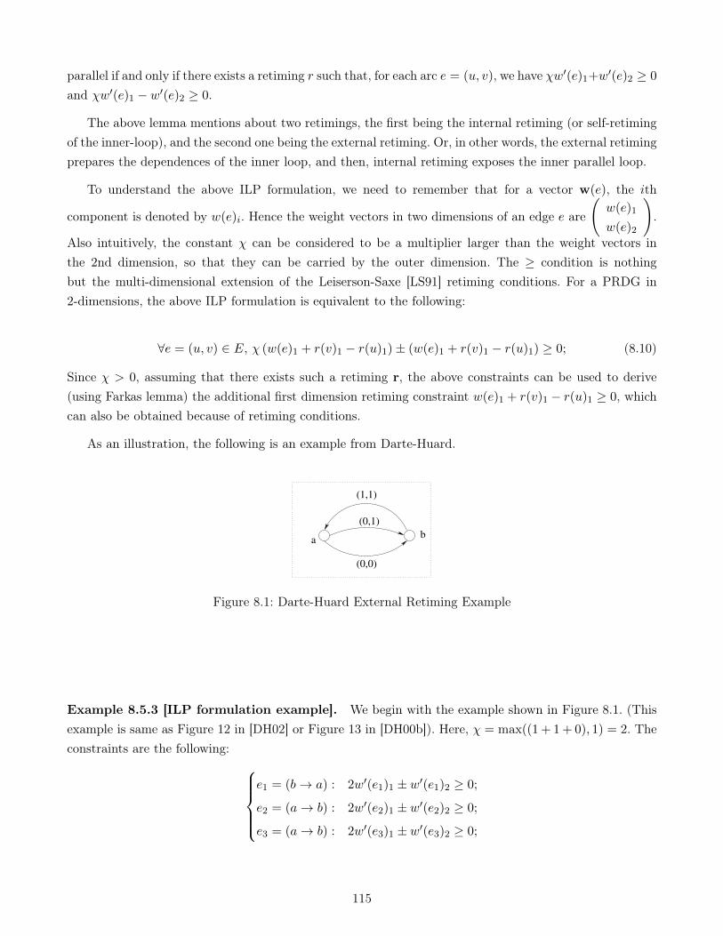
www.dedoimedo.com all rights reserved
parallel if and only if there exists a retiming r such that, for each arc e = (u, v), we have χw′(e)1+w′(e)2 ≥ 0
and χw′(e)1 − w′(e)2 ≥ 0.
The above lemma mentions about two retimings, the first being the internal retiming (or self-retimingof the inner-loop), and the second one being the external retiming. Or, in other words, the external retimingprepares the dependences of the inner loop, and then, internal retiming exposes the inner parallel loop.
To understand the above ILP formulation, we need to remember that for a vector w(e), the ith
component is denoted by w(e)i. Hence the weight vectors in two dimensions of an edge e are
(w(e)1
w(e)2
).
Also intuitively, the constant χ can be considered to be a multiplier larger than the weight vectors inthe 2nd dimension, so that they can be carried by the outer dimension. The ≥ condition is nothingbut the multi-dimensional extension of the Leiserson-Saxe [LS91] retiming conditions. For a PRDG in2-dimensions, the above ILP formulation is equivalent to the following:
∀e = (u, v) ∈ E, χ (w(e)1 + r(v)1 − r(u)1)± (w(e)1 + r(v)1 − r(u)1) ≥ 0; (8.10)
Since χ > 0, assuming that there exists such a retiming r, the above constraints can be used to derive(using Farkas lemma) the additional first dimension retiming constraint w(e)1 + r(v)1 − r(u)1 ≥ 0, whichcan also be obtained because of retiming conditions.
As an illustration, the following is an example from Darte-Huard.
ab
(1,1)
(0,1)
(0,0)
Figure 8.1: Darte-Huard External Retiming Example
Example 8.5.3 [ILP formulation example]. We begin with the example shown in Figure 8.1. (Thisexample is same as Figure 12 in [DH02] or Figure 13 in [DH00b]). Here, χ = max((1 + 1 + 0), 1) = 2. Theconstraints are the following:
e1 = (b→ a) : 2w′(e1)1 ± w′(e1)2 ≥ 0;
e2 = (a→ b) : 2w′(e2)1 ± w′(e2)2 ≥ 0;
e3 = (a→ b) : 2w′(e3)1 ± w′(e3)2 ≥ 0;
115
www.dedoimedo.com all rights reserved
which leads to the following equivalent system, assuming ra =
(ra1ra2
)and rb =
(rb1rb2
)e1 = (b→ a) : 2
(1 + ra1 − rb1
)±(1 + ra2 − rb2
)≥ 0;
e2 = (a→ b) : 2(0− ra1 + rb1
)±(1− ra2 + rb2
)≥ 0;
e3 = (a→ b) : 2(0− ra1 + rb1
)±(0− ra2 + rb2
)≥ 0;
The change in signs in the above system for the r-variables is because of change in directions of the arcs:for e1 it is b→ a, while for e2 and e3 it is a→ b. The above system is equivalent to the following:
e1 : +2ra1 − 2rb1 + ra2 − rb2 + 3 ≥ 0; +2ra1 − 2rb1 − ra2 + rb2 + 1 ≥ 0;
e2 : −2ra1 + 2rb1 − ra2 + rb2 + 1 ≥ 0; −2ra1 + 2rb1 + ra2 − rb2 − 1 ≥ 0;
e3 : −2ra1 + 2rb1 − ra2 + rb2 ≥ 0; −2ra1 + 2rb1 + ra2 − rb2 ≥ 0;
(8.11)
Darte-Huard suggest that the above ILP formulation can be solved using standard ILP solvers. Also, they
suggest the following retimings: ra =
(ra1ra2
)=
(0
0
)and rb =
(rb1rb2
)=
(1
1
)as a possible solution.
It can be seen by substitution that these values satisfy the system in Equation 8.11. �
8.5.3 Heuristics and approximations
For a retiming problem of d-dimensions, the above problem formulation by Darte and Huard has d|V |variables and 2d|E| constraints. But, it can be noticed that the above ILP formulation is constructed ona per-dependence-edge basis and has 4 non-zero variables per constraint. Also, the constraints are general(not just {0,±1}) because of the χ-coefficients. The above system leads to a variety of heuristics andapproximations.
First we begin with some heuristics suggested by Darte and Huard:
Heuristic 8.5.4 [Heuristics of Darte-Huard]. (i) Beginning from the innermost loop till the outer-most loop, use internal shifting on a per-loop basis, exposing as many parallel loops at each individuallevel. (ii) Use Bellman-Ford on the outer loops to expose zero-weight edges on each innerloops.
Of the above methods, (i) can be done in linear time because of the strategy suggested by Darte-Huardwhere the directions of the edges are obliterated by using cycles instead of circuits, and using a depth-first-scan based algorithm to expose parallelism. Also, (ii) can be done in a very affordable O(|E||V |)worst-case time. More details are in [DH00b]. The above methods are inexpensive, but are not as powerfulas ones based on external retiming. The cases when they work may be limited.
We can also have the following approximation using a LP rounding scheme.
Approximation 8.5.5 [LP relaxation]. A simple approximation would be to relax the ILP programof Darte-Huard in Equation (8.10) into an LP program. The resulting rational LP constraints could besolved in polynomial time using the simplex algorithm. Indeed, rational relaxation of an ILP formulation
116
www.dedoimedo.com all rights reserved
and LP-rounding of the rational solution to obtain an integer point for the original problem has been astandard way in which approximation algorithms of NP-Complete problems has been designed [Vaz01].
But, the above approach has the limitation of needing a proper rounding scheme which preserves thelegality of the resultant rational retimed graph. A legal rational retiming can directly be applied to Gfollowed by an expansion of G, but, it solves the retiming of the expanded graph, not of the originalgraph. Also, such an expansion has the undesired side-effect of increasing the code size. Furthermore, theLP-relaxation may be quite expensive to solve as well, with no guarantee of worst-case running time.This is particularly true because of the large size (2d|E| × d|V |) of the LP formulation, which takes up toO(d3|E|2|V |) ≈ O(|V |5) time assuming the observed time of simplex algorithm for bounded d.
The above limitations of a straightforward LP-relaxation leads to the following approximation usingUTVPI-UAs.
Approximation 8.5.6 [Rational (U)TVPI-UA as heuristic]. A heuristic for Darte-Huard’s for-mulation that builds on our approximation techniques is one that UTVPI-UAs each per-edge constraintsand solves the overall system using Bellman-Ford algorithm. This is valid because rational relaxation andsubsequent UA will result in fewer integer points, but no new ones. The overall UA, if non-empty, canbe solved in polynomial time. Since the sparsity of the input system is small and constant (= 4), the(U)TVPI systems have about d|V | variables and 16d|E| constraints. The UTVPI systems, or equivalentlytheir difference constraint MUTVPI approximations, can be solved in O(d2|E||V |) worst-case time, whichis around O(|E||V |) worst-case time for bounded d.
The above approximation comes with a guarantee of bounded cubic worst-case running time, but doesnot come with a guarantee of non-emptiness of the resultant polyhedron. Also, the question of rationalretiming still remains unresolved, which leads to the following approximation.
Approximation 8.5.7 [Integer UTVPI-UA as heuristic]. This approximation is the same as Ap-proximation 2, but uses the integer scaling discussed earlier so as to directly result in an integer multi-dimensional shift. In this method, an ILP problem is solved on a per-Pe-basis, while solving a normalBellman-Ford problem on the overall UA polyhedron resulting in an integer multi-dimensional shift.
Such a polynomial time shifting algorithm is not possible even with a TVPI-UA, as solving integer-TVPI polyhedra is known to be NP-Complete by the result of Lagarias [Lag85].
Validity of UTVPI-UA heuristic It should however be noted that the claim in the above UA-based heuristics (Approximations 8.5.6–7) is quite different from the claim made in the algorithm givenin [SLP96]. In this latter paper, the authors give a polynomial time algorithm for shifting for fusionby formulating an LP problem with difference constraints, and propose to solve the resulting systemusing Bellman-Ford algorithm which has worst-case cubic running time. Furthermore, the authors claim(Theorems 3,12 of [SLP96]) that their algorithm always finds such a retiming function. As the externalshifting problem has been proved by Darte-Huard to be NP-Complete, unless P = NP , the claimedpolynomiality of the above result is invalidated by Darte-Huard’s result.
117

www.dedoimedo.com all rights reserved
Our above claim on the other hand is much weaker because it is just a heuristic. Also, our ap-proximations can be considered to be similar to, as well as an extension of heuristics given by Darte-Huard [DH02, DH00b], where linear or Bellman-Ford based heuristics are given. Furthermore, note thatthe above approximation could result in UAs that are empty when run on a per-dependence edge basis.
Feasibility preservation. We propose some methods by which the problem of feasibility of the TVPI-UA could be solved:
1. One-shot UA-method: Running a one-shot algorithm on all the constraints obviously guaranteesthat the per-dependence UA is feasible, but still does not provide a guarantee that the overallintersection of per-dependence UAs is non-empty.
2. Fixing the sign of the retiming vectors: One limitation of the TVPI approximations is thatthey are sign unaware and the approximation spans too many orthants. To alleviate this problem,the sign of the retiming vectors could be fixed a priori: namely by redefining each retiming vectorr = (r+ − r−), with r+, r− ≥ 0. By this assignment, followed by fixing one of the r+ or r− to be 0
so that the resultant retiming constraints are of the form∑airi + c ≥ 0 where ai is a non-negative
constant, then it could be ensured that the overall UA space spans only the positive orthants andhence is non-empty (this method can be considered to be a rotation of the orthants so that the polarvectors are in one single positive space).
3. Seeding method for UTVPI-Approximations: For feasibility guarantee of the constraint sys-tem, we need to observe that the variables in the constraint system are the components of theretiming vectors. The origin is always a feasible retiming; and a retiming of 0 at each of the verticesof the PRDG is always a valid retiming with the retimed graph corresponding to the original pro-gram. If this seed value is preserved in each of the per-dependence UAs, the overall intersection ofthe per-dependence UAs will have this point as well as (hopefully) other interesting points, whichcan be searched for by the Bellman-Ford algorithm.
Empirical evidence is needed to determine the efficacy of the above methods in practical problems and thecorresponding improvement on running times. As in Darte-Vivien, we are not aware of any implementationof the above algorithm.
8.6 Darte-Huard’s Array Contraction and other ILP problems
Darte and Huard [DH05] show the NP-Completeness of two problems Loop Fusion for array contractionand Loop Shifting for array contraction. In this section, we show that both the formulations by Darte-Huard are amenable to using our framework in multiple ways: under-approximation or enumeration withthe basic engine being a strongly polynomial time UTVPI solver.
118
www.dedoimedo.com all rights reserved
8.6.1 Loop fusion for array contraction
In loop fusion for array contraction, Darte-Huard give the following exact ILP formulation. Let G = (V,E)
be the dependence graph annotated by uniform dependence distances—with the non-uniform dependenceshandled in an appropriate way, like uniformization—and let A be the set of array variables. Also, theydefine simple conditions which classify each arc e as contractable or not. An arc e = (u, v) ∈ E iscalled fusion-preventing if it is annotated by a negative dependence distance; this means that source uand destination v should be placed in different loops, and the source in a loop textually before. An arce = (u, v) ∈ E with a non-negative distance is not fusion preventing; the source should be placed in a loopbefore the destination, or it can be placed in the same loop. The overall resultant of this variety of fusionpartition is a parition of vertices V into disjoint subsets, as long as they sasisfy legality conditions. Darteand Huard suggest the following ILP formulation for the same:
min∑
a∈A δa
subject to
if e = (u, v) ∈ E is not fusion preventing ρv ≥ ρuif e = (u, v) ∈ E is fusion preventing ρv ≥ ρu + 1
if e = (u, v) ∈ E is fusion preventing Nδa ≥ ρv − ρu
(8.12)
It can quickly be noticed that in the above ILP formulation: (i) δa is a binary variable representing whetherthe array variable a ∈ A can be contracted or not; (ii) N is a constant and is heuristically set to numberof edges; (iii) the cost function minimizes the number of contractable arrays.
UTVPI Under-Approximations using enumeration. For designing an approximation or enumera-tion strategy for the above formulation, we have to observe that the δ-variables are binary variables anddefine the cost function. If these variables are set, the rest of the polyhedron induces a UTVPI polyhedron,which can be solved using Bellman-Ford. The δ-variables could be iterated upon with their range simplybeing 0 . . . |A|. The above strategy gives rise to a very straightforward enumeration method using UTVPIpolyhedra. Since the objective is to minimize the number of accesses, the enumeration can proceed byincreasing the array variables that are to be contracted, in a sequential manner.
8.6.2 Loop shifting for array contraction
In their second ILP formulation, Darte-Huard give an ILP formulation for loop shifting for array con-traction, that extends the above formulation for array contraction and their earlier formulation for multi-dimensional shifting [DH02], which was studied in Section 8.5. Hence, the approximation-strategies listedin Section 8.5, as well as and enumeration strategy listed in Section 8.6.1 can be applied to design heuristicsor enumeration methods. The quality of result is equivalent by construction.
119
www.dedoimedo.com all rights reserved
8.6.3 Other 0-1 ILP problems: weighed loop fusion
Darte and Huard’s above mentioned fusion models [DH05] are more powerful than the ones by Songet al. [SXWL01]. Also, Darte and Huard’s models for contraction rectify, and make precise the NP-Completeness result for weighed loop fusion by Kennedy and Mckinley [KM94].
Darte and Huard [DH05] also extend the models of Megiddo and Sarkar [MS97] for the weighed loopfusion problem. This latter paper by Megiddo and Sarkar also has ILP formulation, with a correspondingLP relaxation. Furthermore, they show that a simplification of this LP relaxation has a Totally-Unimodularconstraint matrix and hence admits strongly polynomial time solutions. We study these formulationsbecause of their relevance to our work.
Megiddo-Sarkar’s input model. The input to Megiddo-Sarkar’s algorithm is a directed (but acyclic)graph, called Loop Dependence Graph LDG, whose vertices are perfectly nested loops and whose edgesare dependences (data dependences, like array variables) from the source loop vertex to target loop vertex.Though the input model of Megiddo-Sarkar is quite weak when compared to the other formulations in thischapter–like Darte-Huard’s formulation [DH05]–but it will be elaborated upon because of their use of LPrelaxations of ILP formulations and TU approximations of the same.
Megiddo and Sarkar denote by C ⊆ E, as the set of ordered pairs of vertices (“contractable arcs”) andB the set of unordered pairs of nodes (pairs of nodes that have non-zero weight but are not connected bya summary arc). They formulate an ILP formulation (Problem 3.5 of Megiddo and Sarkar [MS97]) andthen give approximations and relaxations. Also, using a series of transformations, they convert the aboveformulation into the following (Problem 6.3 of Megiddo and Sarkar [MS97]). Let εij ∈ {−1, 1} for every(i, j) ∈ B. A constant εij is chosen a priori for edge (i, j), and π-variables are to be found out.
Lemma 8.6.1 [LP relaxation of [MS97]]. The following LP formulation gives a solution to the π-variables:
minπ∑
(i,j)∈B∪C εijwij(πj − πi) +∑
(i,j)∈C wij(πj − πi)
subject to
πi − πj ≥ 1 ((i, j) ∈ NC)
πi − πj ≥ 0 ((i, j) ∈ C)
(πj − πi)εij ≥ 0 ((i, j) ∈ B)
(8.13)
Megiddo-Sarkar’s formulations and UTVPI approximations. Megiddo and Sarkar claim that theabove LP relaxation in Equation (8.13) is TU, which means that it can directly result in an optimal solutionin strongly polynomial time. Instead, the LP-relaxation and its UTVPI approximation will be a directconsequence of using our approaches in this dissertation, and more particularly in this particular chapter;the suggestion above is directly advocating for our UTVPI, and consequently MUTVPI, approximationapproaches.
120
www.dedoimedo.com all rights reserved
8.7 A General UA-Framework of Loop Transformation Polyhedra
UA framework. The formulations seen above in this chapter, there is a common pattern of formulatingmixed 0− 1-ILP problems, where some variables (x) are restricted to rationals (Q), some (y) to integers(Z), while the rest (δ) to binary ({0, 1}) decision values. We use this insight to develop a general frameworkfor MILP approximation that is particularly suited for loop transformation polyhedra: polyhedra whosesolutions are valid affine loop transformations.
For this let us consider the general set of scheduling constraints:
min∑
c(x,y, δ)
subject to Ax +By + Cδ ≤ d
x ∈ Qnx ; y ∈ Zny ; δ ∈ {0, 1}nδ
(8.14)
where A,B,C are constraint matrices and x,y, δ are the variables of the scheduling problem. c is a linearcost function specific to the problem at hand.
We can use this above generic MILP formulation to design under-approximation algorithms for loopscheduling or affine transformation problems. We use Table 8.2, to characterize the different problems andtheir complexities. We use the notation of Section 3.4 on page 30: SPT means strongly polynomial Time,WPT means Weakly Polynomial Time because the algorithm has been reduced to LP, and NPC meansthat the problem is NP-Complete.
Using the above notation, Calland et al. [CDR98] and Darte and Huard [DH00a] use TU properties ofA to formulate a (strongly) polynomial time algorithm. This is possible because A is derived using G.
Similarly, Darte and Vivien [DV97a] formulate an LP formulation, which, though using binary decisionvariables, takes weakly polynomial time. Feautrier [Fea92a, Fea92b] and FCO of Griebl et al. [GFG02,BHRS08] formulate weakly polynomial time LP based algorithm, where the x-variables are constructedusing Farkas multipliers. Feautrier’s multi-dimensional scheduling and the FCO scheduling use appropriatebinary decision variables, though the overall algorithm taking weakly polynomial time. In a similar way,Lim-Lam [LL97] and Thies et al. [TVA07], use a similar framework, though for purposes of synchronizationfree parallelism and memory optimization respectively.
Darte and Huard [DH02] formulate NP-Complete problems where y-variables are constructed usingthe retiming vectors. Darte and Huard [DH05] build from the above formulation and the structure of thegraph to formulate a 0− 1 ILP formulation for the NP-Complete problems of array contraction.
UA strategies. Broadly, using the above framework, we can design UA strategies so that each of theabove problems can be solved with a low worst-case polynomial complexity: This can be done in threedifferent ways: (i) relaxing all 0 − 1 variables and integer (Z) variables to rationals (Q), and finding aUA in a relaxed framework; (ii) replacing the Q-polyhedron by its UA, followed by enumeration of the0 − 1 variables; (iii) separating the overall Q-polyhedron to smaller scalable sub-problems that can beunder-approximated using graph theoretical properties.
121
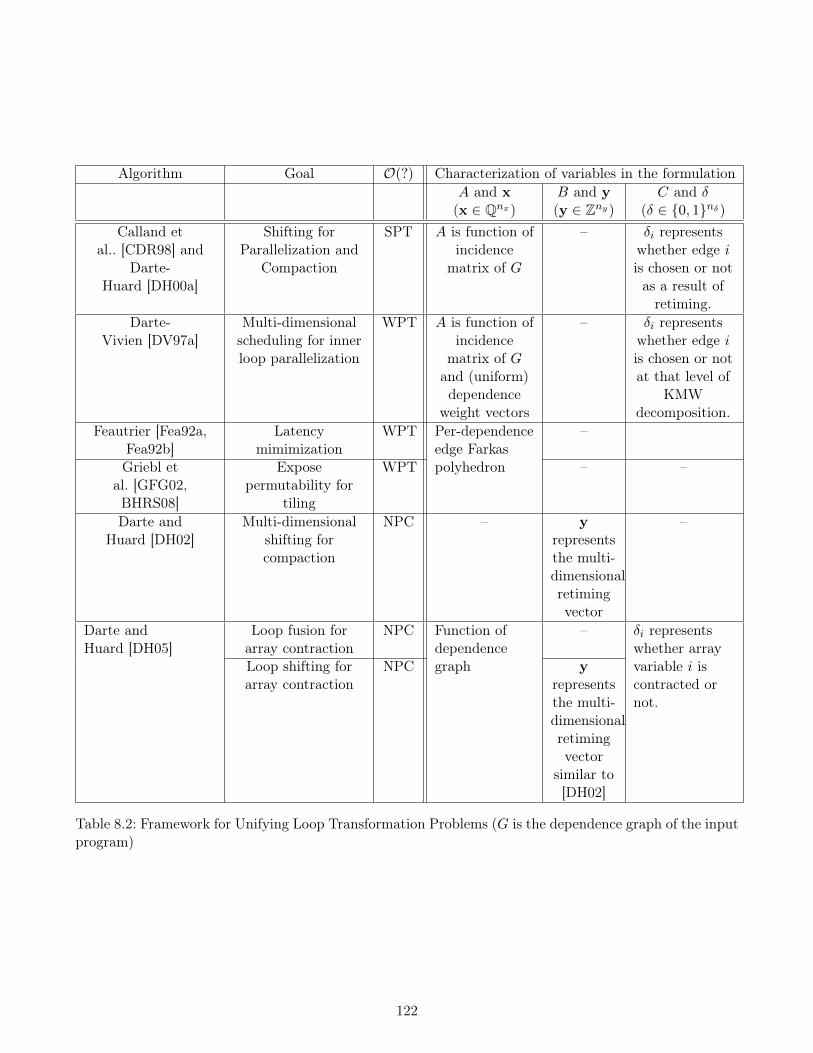
www.dedoimedo.com all rights reserved
Algorithm Goal O(?) Characterization of variables in the formulationA and x(x ∈ Qnx)
B and y(y ∈ Zny)
C and δ(δ ∈ {0, 1}nδ)
Calland etal.. [CDR98] and
Darte-Huard [DH00a]
Shifting forParallelization and
Compaction
SPT A is function ofincidence
matrix of G
– δi representswhether edge iis chosen or notas a result ofretiming.
Darte-Vivien [DV97a]
Multi-dimensionalscheduling for innerloop parallelization
WPT A is function ofincidence
matrix of Gand (uniform)dependence
weight vectors
– δi representswhether edge iis chosen or notat that level of
KMWdecomposition.
Feautrier [Fea92a,Fea92b]
Latencymimimization
WPT Per-dependenceedge Farkaspolyhedron
–
Griebl etal. [GFG02,BHRS08]
Exposepermutability for
tiling
WPT – –
Darte andHuard [DH02]
Multi-dimensionalshifting forcompaction
NPC – yrepresentsthe multi-dimensionalretimingvector
–
Darte andHuard [DH05]
Loop fusion forarray contraction
NPC Function ofdependencegraph
– δi representswhether arrayvariable i iscontracted ornot.
Loop shifting forarray contraction
NPC yrepresentsthe multi-dimensionalretimingvector
similar to[DH02]
Table 8.2: Framework for Unifying Loop Transformation Problems (G is the dependence graph of the inputprogram)
122
www.dedoimedo.com all rights reserved
A combination of the above methods could also be used. Even when the UA methods of is not ef-fective, it could give rise to an effective enumeration strategy that could be used. Briefly, relaxation hasalready been used in Calland et al. [CDR98] and Darte and Huard [DH00a]. Relaxing y to rational vari-ables followed by (U)TVPI approximation has been suggested for Darte and Huard’s multi-dimensionalscheduling [DH02]. Enumeration on δ-variables using the UA of the relaxation could be used for any NP-Complete problems with ILP/MILP formulations. Furthermore, the unit-schedule (canonical schedule)preserved in the UA could be used for a feasibility preservation.
8.8 Schedules with no Modulos
We state in Section 6.7.5, that thanks to the Totally Unimodular(TU) property, a restriction of thehomogenizing dimensions to integers can ensure that all the vertices of the resultant UTVPI-UA areintegers. In this method, the under-approximation is again performed on a per-dependence basis, thoughwith the additional restriction that the homogenizing dimension of the under-approximation is integer.This latter restriction is possible by scaling the homogenizing dimension choices along with appropriatepseudo-parametric values, and making an ILP call, rather than the usual LP call per-dependence. Theoverall result is a UTVPI approximation.
Because of the TU property, this latter approximation is a polyhedron with integer vertices. Whenusing these UAs in scheduling, the primary advantage is that the schedule can be found in stronglypolynomial time with very low O(mn) complexity; it has the additional advantage of simpler code beinggenerated, even with affine schedules obtained as a result of (rational) linear programming. The FCOscheduler in PLuTo uses integer linear programming by default for the same purpose, and such a use couldbe expensive. Rational schedule coefficients may indeed induce modulos in loop bounds and conditionalexpressions of the generated code. This is eliminated by such an a priori restriction of the schedules.
123
www.dedoimedo.com all rights reserved
8.9 Conclusions and Perspectives
We review the conclusions and contributions of this chapter and summarize some related work.
Conclusions
In this chapter, we have provided a preliminary idea on how the under-approximation strategies developedin earlier chapters could be applied to various scheduling problems in loop optimization. We began withthe simplest case of problems [CDR98, DH00a] that have already been reduced to strongly polynomialtime. This was followed by more general transformations [DV97a, Fea92a, Fea92b, GFG02, BHRS08] thatare linear programming based and hence have a weakly polynomial time complexity. This was furtherfollowed by special case transformations [DH02, DH05], which are computationally much harder problemsbecause of their NP-Completeness reductions. We suggested heuristics, approximation and enumerationstrategies on a case by case basis. The methods should be seen as initial approaches on how UA methodscould be applied, with more study being needed.
Contributions
Under approximation of scheduling problems. We think that this is perhaps the first system-atic and algorithmic approximation scheme to be applied to formulations in loop scheduling. Firstly,we studied a gradation of problems: according to the type of loop transformations they target (1d-transformations, more general nd-transformations, or specific nd-transformation), and according to theiralgorithmic complexity—strongly polynomial time, weakly polynomial time, or NP-Complete). Each ofthese transformations could benefit from the under-approximation methodology developed in the previouschapters.
Though we have suggested for some NP-Complete problems, it could even be used with more recent andmore powerful techniques as well. This means the fusion in the presence of hardware and other constraintsby Bondhugula et al. [BGDR10], and the complete convex characterizations of loop transformations byPouchet et al. [PBB+11]. Each of these could benefit from our framework, where the rational part issimplified (UA’d) to a (U)TVPI polyhedron in a preprocessing step, before the actual solution step.
Parts of the experiments (clustering techniques) and some of the applications listed in this chapterhave been presented in [UC13].
Scheduling amenable to code generation. In Section 8.8, we had suggested a very preliminarymethod in which the schedule module of the polyhedral code generation is made aware of the latter codegeneration module. This can be considered to be in the same spirit of Darte and Vivien [DV97a] andDarte and Huard [DH02] who hint that more complicated schedules may not practically yield sufficientadvantage because the code generated for those schedules may be very complicated. But, as far as weare aware of, this aspect of exploiting Totally-Unimodularity has not been previously approached in loopoptimization. The approach in this section should however be seen as different from the approach in the
124

www.dedoimedo.com all rights reserved
following chapter (Chapter 9), where the complexity of the code generaton is independently reduced topolynomial time using the complexity guarantee of (U)TVPI polyhedra.
Limitations
The under-approximation methods are limited in a couple of ways: feasibility and practical effectiveness.For many of the applications in this chapter, more study of the preservation of feasibility via the preser-vation of the unit schedule is needed. Furthermore, most of the applications in this chapter need moreempirical study regarding their effectiveness.
Feasibility and effectiveness. In particular, the approximations for the 1d-transformations [CDR98,DH00a] and even more general transformations like Darte-Vivien [DV97a] may not be practically sig-nificant because of the restricted practicability of the original formulations. However, the insights givenby these original formulations and the approximation or enumeration techniques are significant to beapplicable to problems of greater use and complexity. Feautrier’s formulation [Fea92a, Fea92b], FCO for-mulation [GFG02, BHRS08], and the NP-Complete formulations of Darte and Huard [DH02, DH05] aresuch problems.
Even though the effectiveness of these latter three applications may also be limited, and the approxi-mation or enumeration techniques suggested may be too simple to begin with, it is hoped that the ideaspresented here will lead to a new method to derive approximation algorithms for loop transformationproblems. In this sense, the effectivenss of the approximations is related to finding approximations toNP-Complete problems by Hochbaum [HMNT93, Hoc04].
Improvement of methods. Lack of the feasibility guarantee of the approximations is a limitation.It could be overcome using the idea of preservation of canonical schedules suggested many times in thechapter. Furthermore, the constraints or the dependences could be grouped using clustering techniquessimilar to those suggested in Section 8.4.2.. Finally, some of the enumeration strategies given here havethe severe limitation that they do not have a polynomial time guarantee. They can however be improvedby studying the particular problem carefully, as indicated in Section 8.7.
From Chapter 4 till the current chapter, we applied the (U)TVPI sub-polyhedra based under-approximationtechniques to affine scheduling problems. In this chapter, the application was extended to a variety of affinetransformation problems. In the next chapter, we change tracks by applying the use of (U)TVPI polyhedrato the polyhedral code-generation problem.
125

www.dedoimedo.com all rights reserved
126

Chapter 9
An Approach for Code Generation using(U)TVPI Sub-Polyhedra
In this chapter, we explore how we can use TVPI polyhedra for sequential code generation, with a goalof polynomial time complexity guarantee. Though our goal is to solve the code generation problem, theproblem we actually solve is a sub-problem: that of polyhedra scanning using TVPI sub-polyhedra. Thedifference between the two is that the latter scanning problem does not need to take care of how theimperfectly nested loops are encoded, how the code for the statements in the loop (loop body) is encodedetc.
9.1 Introduction
Beginning from a schedule—possibly a multi-dimensional schedule—for a set of input statements, theproblem of code generation is loosely defined to finding a scanning order by touching each integer point inthe domains exactly once, while respecting the dependences between the statements. For serial code, thescanning order means to generate for loops for the input domains. In this chapter, we will propose TVPIbased methods for doing the same in asymptotically polynomial time using TVPI properties.
Structure of this introduction. For doing the above, we would first quickly summarize the currentcode generation methods in Section 9.1.1. This will be followed by Section 9.1.2, where we will identifythe problem in code generation to be the exponentialities in the algorithm by Quilleré et al. [QRW00].This will be followed by listing of the goals and some hypothesis in Section 9.1.3, followed by showing thepotential of TVPI polyhedra in Section 9.1.4.
127

www.dedoimedo.com all rights reserved
9.1.1 A summary of current code generation methods
Very broadly, the three main methods of polyhedral code generation are based on the geometric algorithmsof Fourier-Motzkin (FM), Parametric Integer Programming (PIP) and separation of polyhedra. Threeprimary metrics are used to evaluate these methods: the size of the generated code, the execution time ofthe code generator, and the execution time of the generated code.
FM based method. The FM based methods are based on the seminal work of Ancourt and Irigoin [AI91],who suggested using Fourier-Motzkin algorithm for generating the loop bounds for the for loops. The mainintuition of this method is to use the projection method of FM to each of the individual dimensions. Theresultant bounds of each loop index are affine terms of the outer dimensions and the parameters and canbe used to generate the bounds of their corresponding loops. This method has been extended by manyresearchers for the cases of multiple polyhedra and statements cases.
A primary limitation of FM is the algorithm itself, that is known to take worst-case doubly exponentialtime because of the large number of redundant constraints that are generated. Inspite of good implemen-tations in libraries like FMLib [Pou] and Omega [Pug91], the algorithm has a doubly exponential timecomplexity. Also, the main limitation of the FM based methods is not only its time complexity, but alsothe inactive or redundant areas in the generated code. This is a directl result of the redundant constraintsgenerated by the algorithm.
An implementation of this method improved with a redundancy eliminating mechanism has beensuggested by Kelly, Pugh and Rosser [KPR95] and exists in the Omega library. This code generator,CodeGen, is one of most widely used and has recently been improved by the work of Chen [Che12] inOmega 2.0 to CodeGen+. This latter improvement is discussed in the related work section at the end ofthis chapter.
PIP based method. The PIP based method are the work of Boulet and Feautrier [BF98]. This latteralgorithm is based on the intuition that the successive integer points that have to be scanned can be foundas a result of integer programming lexmins, and these calls can further be parametrized. Similar to the FMbased methods, the PIP methods still generates redundant control and even needs to duplicate code. Themethod is based on the PIP [Fea88], but, there is no widely used implementation of this method for thecase of multiple polyhedra. So, it is not known how it practically fares on real benchmarks. Furthermore,it does not aim to generate high-level loop statements like the other tools.
Separation based method (QRW algorithm). The separation based methods started with the al-gorithm by Quilleré, Rajopadhye and Wilde [QRW00], called the QRW method. The QRW method is theonly method of the above three methods which can generate exact code with non-redundant control. Thisalgorithm has been extended and implemented in CLooG [Bas04a, Bas04b] and is the most widely usedamong the above three algorithms. The main intuition of this method is based on separation of polyhedraand their projections. The algorithm is given in a simplified form [Bas11, Bas12] in Figure 9.1.
128
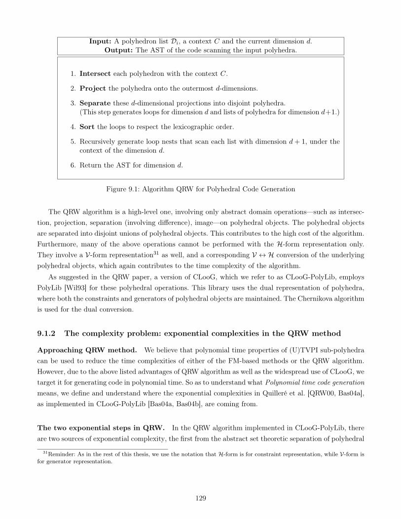
www.dedoimedo.com all rights reserved
Input: A polyhedron list Di, a context C and the current dimension d.Output: The AST of the code scanning the input polyhedra.
1. Intersect each polyhedron with the context C.
2. Project the polyhedra onto the outermost d-dimensions.
3. Separate these d-dimensional projections into disjoint polyhedra.(This step generates loops for dimension d and lists of polyhedra for dimension d+1.)
4. Sort the loops to respect the lexicographic order.
5. Recursively generate loop nests that scan each list with dimension d+ 1, under thecontext of the dimension d.
6. Return the AST for dimension d.
Figure 9.1: Algorithm QRW for Polyhedral Code Generation
The QRW algorithm is a high-level one, involving only abstract domain operations—such as intersec-tion, projection, separation (involving difference), image—on polyhedral objects. The polyhedral objectsare separated into disjoint unions of polyhedral objects. This contributes to the high cost of the algorithm.Furthermore, many of the above operations cannot be performed with the H-form representation only.They involve a V-form representation31 as well, and a corresponding V ↔ H conversion of the underlyingpolyhedral objects, which again contributes to the time complexity of the algorithm.
As suggested in the QRW paper, a version of CLooG, which we refer to as CLooG-PolyLib, employsPolyLib [Wil93] for these polyhedral operations. This library uses the dual representation of polyhedra,where both the constraints and generators of polyhedral objects are maintained. The Chernikova algorithmis used for the dual conversion.
9.1.2 The complexity problem: exponential complexities in the QRW method
Approaching QRW method. We believe that polynomial time properties of (U)TVPI sub-polyhedracan be used to reduce the time complexities of either of the FM-based methods or the QRW algorithm.However, due to the above listed advantages of QRW algorithm as well as the widespread use of CLooG, wetarget it for generating code in polynomial time. So as to understand what Polynomial time code generationmeans, we define and understand where the exponential complexities in Quilleré et al. [QRW00, Bas04a],as implemented in CLooG-PolyLib [Bas04a, Bas04b], are coming from.
The two exponential steps in QRW. In the QRW algorithm implemented in CLooG-PolyLib, thereare two sources of exponential complexity, the first from the abstract set theoretic separation of polyhedral
31Reminder: As in the rest of this thesis, we use the notation that H-form is for constraint representation, while V-form isfor generator representation.
129
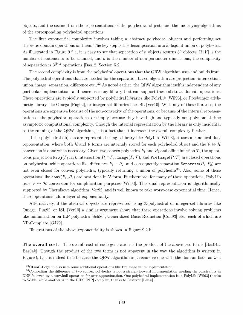
www.dedoimedo.com all rights reserved
objects, and the second from the representations of the polyhedral objects and the underlying algorithmsof the corresponding polyhedral operations.
The first exponential complexity involves taking n abstract polyhedral objects and performing settheoretic domain operations on them. The key step is the decomposition into a disjoint union of polyhedra.As illustrated in Figure 9.2.a, it is easy to see that separation of n objects returns 3n objects. If |V | is thenumber of statements to be scanned, and d is the number of non-parameter dimensions, the complexityof separation is 3|V |d operations [Bas12, Section 5.2].
The second complexity is from the polyhedral operations that the QRW algorithm uses and builds from.The polyhedral operations that are needed for the separation based algorithm are projection, intersection,union, image, separation, difference etc.,32 As noted earlier, the QRW algorithm itself is independent of anyparticular implemetation, and hence uses any library that can support these abstract domain operations.These operations are typically supported by polyhedral libraries like PolyLib [Wil93], or Presburger arith-metic library like Omega [Pug92], or integer set libraries like ISL [Ver10]. With any of these libraries, theoperations are expensive because of the non-convexity of the operations, or because of the internal represen-tation of the polyhedral operations, or simply because they have high and typically non-polynomial-timeasymptotic computational complexity. Though the internal representation by the library is only incidentalto the running of the QRW algorithm, it is a fact that it increases the overall complexity further.
If the polyhedral objects are represented using a library like PolyLib [Wil93], it uses a canonical dualrepresentation, where both H and V forms are internaly stored for each polyhedral object and the V ↔ Hconversion is done when necessary. Given two convex polyhedra P1 and P2 and affine function T , the opera-tions projection Proj(P1, xi), intersection P1∩P2, Image(P, T ), and PreImage(P, T ) are closed operationson polyhedra, while operations like difference P1 − P2, and consequently separation Separate(P1, P2) arenot even closed for convex polyhedra, typically returning a union of polyhedra33. Also, some of theseoperations like conv(P1, P2) are best done in V-form. Furthermore, for many of these operations, PolyLibuses V ↔ H conversion for simplification purposes [Wil93]. This dual representation is algorithmicallysupported by Chernikova algorithm [Ver92] and is well known to take worst-case exponential time. Hence,these operations add a layer of exponentiality.
Alternatively, if the abstract objects are represented using Z-polyhedral or integer-set libraries likeOmega [Pug92] or ISL [Ver10] a similar argument shows that these operations involve solving problemslike minimization on ILP polyhedra [Sch86], Generalized Basis Reduction [Coh93] etc., each of which areNP-Complete [GJ79].
Illustrations of the above exponentiality is shown in Figure 9.2.b.
The overall cost. The overall cost of code generation is the product of the above two terms [Bas04a,Bas04b]. Though the product of the two terms is not apparent in the way the algorithm is written inFigure 9.1, it is indeed true because the QRW algorithm is a recursive one with the domain lists, as well
32CLooG-PolyLib also uses some additional operations like PreImage in its implementation.33Computing the difference of two convex polyhedra is not a straightforward implementation needing the constraints in
DNF followed by a conv.hull operation for over-approximation. One polyhedral implementation is in PolyLib [Wil93] thanksto Wilde, while another is in the PIPS [PIP] compiler, thanks to Leservot [Les96].
130

www.dedoimedo.com all rights reserved
Separate (S1, S2) = {S1 − S2, S1 ∩ S2, S2 − S1}
Separate (S1, S2, S3) =
S1 − S2 − S3, . . . ,S3 − (S1 − S2), . . . ,S3 − (S1 ∩ S2), . . . ,(S1 ∩ S2)− S3, . . . ,
S1 ∩ S2 ∩ S3
{P1 ∩ P2 ≡ PH1 ∩ PH2P1 ∪ P2 ≡ PV1 ∪ PV2
(a) Separation of n abstract objects into their disjointunion resulting in an exponential size output
(b) Operations on polyhedra needexpensive algorithms like
Chernikova, resulting in exponentialtime.
Figure 9.2: Illustration of the two exponentialities associated with QRW algorithm, when it uses PolyLibfor representation of its polyhedral objects.
as the context passed as parameters from dimension d to d + 1. A separation at dimension d gives morepolyhedral objects to be processed in the higher dimensions. Furthermore, the list of polyhedra processedat dimension d needs to be processed by a V ↔ H conversion because of the operations in the nextdimension d+ 1: separation at step d which is best done with V-form is followed by an intersection at stepd+ 1 which is best done with H-form.
Our reduction of exponential cost of code generation to polynomial time is based on CLooG-PolyLibimplementation, which uses the PolyLib library for representation of its polyhedral objects. In this chap-ter, we would be referring to only CLooG-PolyLib. Hence, we would informally be referring to thesecomplexities as the two exponential complexities in polyhedral code-generation.
9.1.3 Our goal, the inputs and some hypotheses
In this section, we define the goal of this chapter, followed by understanding the restricted variety ofdomains that the sub-polyhedral code-generation algorithms take as inputs. Since there are bound to bedomains which are not of this specific form, we suggest some methods of preprocessing the inputs whichare not of this restricted variety.
TVPI input: The primary goal of this chapter is to analyze and suggest improved QRW-algorithms inthe case when each domain Di is a (U)TVPI domain. Though we will specifically mention TVPI polyhedrain this chapter, many statements are valid for UTVPI polyhedra as well.
Legal input: Each domain Di can be a parametrized domain, but in a limited way. For example, if weconsider indices i, j and parameters M and N , i+ j ≤ 10 is allowed and so are i ≤ N + 10 and M ≤ N ;but i + j ≤ N or i ≤ N + 2M are not. Though this restriction seems limited when compared to generalconvex constraints, constraints like i+2j ≤ 10 as well as i+10 ≤ 2N , which cannot be encoded by interval
131

www.dedoimedo.com all rights reserved
“box” constraints are encoded by TVPI. Since the meaning of variables is known, we refer to constraintswithout distinguishing the indices from the parameters.
There are two ways of managing domains which are not already TVPI:
TVPI over-approximation of domains: Domains which are already not TVPI can be over-approximatedfirst and de-approximated later. This approximation and de-approximation process can happen on a per-statement basis. These over-approximations act like a padding of the domains of the individual statementsso that additional integer points, that do not belong to the actual specified domain of the statement can bescanned. The padding is simplified in a post-processing phase, after the QRW code generation. Since theper-statement domains are likely to be very small constraint systems, the over-approximation algorithmbased on the generator representation could be used. The over-approximation algorithms in Chapter 4.3on page 50, with examples illustrated in Figure 4.3 on page 50 can be used.
Instantiation of parameters. Parameters can be instantiated into constants using extraneous domaininformation. For example, if it is known statically that N < M , then N and M can be assigned constantssufficiently large or sufficiently characteristic of the particular input so that constraints involving N andM can be analyzed as TVPI constraints. For example, constraint i + j ≤ N becomes i + j ≤ 100 andconstraint i − j ≤ M becomes i − j ≤ 200; also, constraint i + j ≤ N + 2M results in the constrainti+ j ≤ 500 with N = 100 ∧M = 200 as instantiation.
9.1.4 Potential of TVPI sub-polyhedra
Suppose we do begin with some of the above mentioned hypotheses: for example, the over-approximation ofeach domain by sub-polyhedra, followed by possible instantiation of parameters so as to reduce the numberof active variables per constraint. The questions we want to answer in this chapter are the following:
• Can we give a guaranteed time complexity for code generation assuming the underlying methodis CLooG-PolyLib implementation of QRW algorithm? For the above, do (U)TVPI sub-polyhedrahelp?
• Is the guaranteed time-complexity polynomial as well (like POLY(Stmts,Constr,Loops) etc.)? Whichof the two exponential steps get reduced to polynomial time complexity and how?
• Since the gain in complexity requires a trade-off in the other metrics of code size and/or generatedcode execution time, what will the (U)TVPI-approximation lose when compared to general convexpolyhedra?
Briefly, the answers to the above questions are: TVPI sub-polyhedra indeed do help in polynomial timecode generation by reducing both of exponential steps to polynomial time. The generated code will beintermediate to, and in between what is generated by a naïve method using interval polyhedra, and themost sophisticated method of QRW as available in CLooG. The loss of precision—measured in terms ofscanning the inactive code—would be due to two reasons: the approximation of non-TVPI domains intoTVPI polyhedra and because of using TVPI sub-polyhedra.
132
www.dedoimedo.com all rights reserved
domains
Closure of thePer−statementdomainsGeneral
...
1 Over−Approximation
...
Separation usingthe projection onthe dth dimension
... ...Separation usingthe planar projectionon the iXd plane
...
De−approximation
Per−dimension method
Post−processsing4
Over−ApproximationAlgorithm
of parameters+Instantiation
2
Two Alternatives in TVPI Code Generation3
...
Planar method
Pre−Processing
domainsTVPIconvex
Figure 9.3: An Overview of Code Generation using TVPI polyhedra (QRW-TVPI)
Our exposition would alternate between the closure properties, graphical representation and geometricproperties of TVPI polyhedra. Here is a brief summary of our approach.
A summary of our approach. We primarily rely on polynomial time geometric and closure operationsoffered by (U)TVPI polyhedra. As discussed in Chapter 3, the polynomial time closure operations let usextend the geometric algorithms developed for planar polyhedra to general TVPI polyhedra. This impliesthat the projection and separation of polyhedral objects, which are the two key polyhedral operations usedby the QRW algorithm, can be performed in guaranteed polynomial time for TVPI sub-polyhedra.
Specifically, we exploit the fact that, while the enumeration of generators of general convex polyhedratakes exponential time because of the inherent nature of generators, the enumeration of the vertices of then(n− 1)/2 planar projections of TVPI polyhedra can be done in polynomial time. If we begin with TVPIsub-polyhedra as domains, we can design algorithms that allow for guaranteed polynomial time projectionand separation operations.
These ideas result in the design of a sub-polyhedral code-generation schema: QRW-TVPI and two con-sequent specializations of the QRW algorithm using TVPI sub-polyhedra: QRW-TVPI1, a per-dimensionalalgorithm with lesser precision but using linear time separation complexity, and QRW-TVPI2, a planar al-gorithm with polynomial time complexity which uses a closure-based separation method. This second onecomes with two specializations: a heuristic-based one with lower precision and a closure-based algorithmwhich provides better control overhead of the generated code.
Our methods are illustrated in Figure 9.3.
133
www.dedoimedo.com all rights reserved
9.1.5 An overview of this chapter
We begin with a quick reminder of the properties of TVPI sub-polyhedra in Section 9.2. This section is arewrite of material in Chapter 3, with some additional key lemmas and remarks.
In Section 9.3, we introduce QRW-TVPI: a TVPI code generation schema based on the polynomialproperties of TVPI polyhedra. This can be used to create two variations of the QRW algorithm each ofwhich provide a guarantee in the complexity. In Section 9.4, we present QRW-TVPI1, which is a simpleper-dimension variation of the method. This is followed in Section 9.5, by the introduction of QRW-TVPI2,a variation of QRW algorithm for TVPI polyhedra. Both these algorithms are small variations of the QRWalgorithm and reduce the two exponential steps in the QRW algorithm to polynomial time.
In Section 9.6, we quickly re-summarize some additional related work. Finally, this chapter is concludedin Section 9.7 with a list of contributions, perspectives and comments about related work.
9.2 TVPI Polyhedra Properties: A Quick Summary
The following result is by Graham [Gra72, dBKS00] (“Graham’s scan” algorithm) shows the polynomialityof finding the vertices of planar polyhedra (polygons). It has been improved by Simon and King [SK04]to the problem of finding the generators (both vertices and rays) of planar polyhedra taking many specialgeometric cases of unbounded polyhedra, lineality space etc., into consideration:
Lemma 9.2.1 [Convex hull of planar H-Polyhedra]. Given a planar polyhedron withm constraints,its generator representation (convex-hull) can be found in worst-case polynomial time O(m logm).
The above very low complexity polynomial time algorithm is to be contrasted with the correspondingexponential time complexity for 3-dimensional and higher dimensional (general convex) polyhedra of theusual Chernikova algorithm [Ver92]. This latter exponential time is not a limitation of the Chernikovaalgorithm, but characteristic of the output itself which could be up to nbm2 c size on non-planar polyhedra.Even the classic interval “box” polyhedra (a hypercube) in n-dimensions which is the simplest case ofsub-polyhedra has an exponential number of vertices. The above complexity result holds true for TVPIsub-polyhedra as well: the problem of enumerating all their vertices takes exponential time.
Polyhedral vs. graphical methods for TVPI polyhedra. It is well known that for general convexpolyhedra, obtaining the exact projections on any 2-dimensional plane34 takes exponential time usingeither of the Chernikova or Fourier-Motzkin methods. But, following the classic works of Shostak [Sho81]and Aspvall and Shiloach [AS80], the breakthrough in TVPI algorithms by Hochbaum and Naor [HN94] isin noticing that the 2-dimensional projections of a TVPI polyhedron can be computed using graph-theorymethods, rather than polyhedral ones. On a 2-dimensional projection, using polyhedral methods, however,does not imply exponential time because of the polynomial complexity of the Graham’s scan algorithm(see above).
34This corresponds to what the Omega paper [Pug92] calls as 2d-dark-shadow.
134

www.dedoimedo.com all rights reserved
Given a general TVPI polyhedron, let the breakpoints be the set of vertices associated with the i-thdimension. In other words, they define the envelopes of each of the i− j planes for 1 ≤ j ≤ n; j 6= i. Thefollowing result is from Hochbaum and Naor [HN94]:
Lemma 9.2.2 [Number of breakpoints]. Given a general TVPI polyhedron with m constraints inn dimensions, the number of polyhedral vertices35 associated with any dimension i is linear in the totalnumber of constraints: O(m). (The actual number is m+ 4n.)
The following result is also by Hochbaum and Naor [HN94].
Lemma 9.2.3 [Fourier-Motzkin on TVPI polyhedra]. The Fourier-Motzkin elimination to deter-mine the feasibility of general TVPI polyhedra—as opposed to planar polyhedra—can be performed instrongly polynomial time with complexity O(mn2 logm).
As noted in Chapter 3, the above result is surprising, because FM is known to take doubly exponentialtime on general convex polyhedra, taking up to bm2 c2
n time. The FM method on TVPI polyhedra is relatedto the following corollary of TVPI polyhedra, again due to Hochbaum and Naor [HN94]:
Corollary 9.2.4 [Projection and TVPI polyhedra]. Given a TVPI polyhedron in n dimensions,projecting out a dimension (variable) results in a TVPI polyhedron in n− 1 dimensions. The complexityof this projection is O(mn logm).
This means that TVPI polyhedra are closed under projection. The intuition for this can be obtainedin a geometric way or a graph theoretical way. The graph theoretic intuition for the same is shown inFigure 9.4. All the TVPI algorithms involve a simple graph-based representation of the TVPI constraintsand a polynomial time closure. This operation is cubic: max(n3,m3).
Closure properties. The closure operation on TVPI polyhedra adds additional constraints to its H-form; these additional constraints can be considered to be all possible projections of the TVPI system.Using this so-called closed system, the projection of the system on the plane xi× xj can be inferred usingonly the constraints in which xi and xj have non-zero coefficients. Furthermore, obtaining the closuresimplifies many operations involving multiple TVPI systems. For example, convex union of two TVPI-systems P1 and P2 can be done by first obtaining the closure of both P1 and P2, followed by performinga planar convex-hull on each of the n(n−1)
2 planar systems, with the overall method having very lowcomplexity. The conventional method on the other hand, would involve finding the V-form of each of thesystems and hence has high computational complexity.
Graph theoretically, as TVPI polyhedra can be represented using directed graphs, closure can be saidto be adding additional directed edges to the graph with specific weight so that the sub-graph inducedby vertices xi and xj can be used to infer the properties between variables xi and xj . This is shown inFigure 9.4.
35Hochbaum and Naor [HN94] refer to these as breakpoints.
135
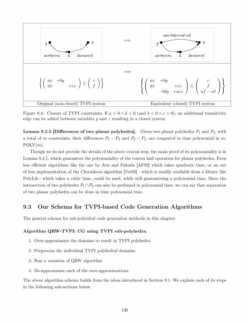
www.dedoimedo.com all rights reserved
dx+ez<=f
z
x
y
ax+by<=c
=⇒aez−bdy<=af−cd
z
x
y
ax+by<=c dx+ez<=f
{(ax +bydx +ez
)≤(cf
)} =⇒ ax +by
dx +ez−bdy +aez
≤ c
faf − cd
Original (non-closed) TVPI system Equivalent (closed) TVPI system
Figure 9.4: Closure of TVPI constraints. If a > 0 ∧ d < 0 (and b < 0 ∧ e > 0), an additional transitivityedge can be added between variables y and z resulting in a closed system.
Lemma 9.2.5 [Differences of two planar polyhedra]. Given two planar polyhedra P1 and P2, witha total of m constraints, their differences P1 − P2 and P2 − P1, are computed in time polynomial in m:POLY(m).
Though we do not provide the details of the above crucial step, the main proof of its polynomiality is inLemma 9.2.1, which guarantees the polynomiality of the convex hull operation for planar polyhedra. Evenless efficient algorithms like the one by Avis and Fukuda [AF92] which takes quadratic time, or an outof box implementation of the Chernikova algorithm [Ver92]—which is readily available from a library likePolyLib—which takes a cubic time, could be used, while still guaranteeing a polynomial time. Since theintersection of two polyhedra P1∩P2 can also be perfomed in polynomial time, we can say that separationof two planar polyhedra can be done in time polynomial time.
9.3 Our Schema for TVPI-based Code Generation Algorithms
The general schema for sub-polyedral code generation methods in this chapter:
Algorithm QRW-TVPI: CG using TVPI sub-polyhedra.
1. Over-approximate the domains to result in TVPI polyhedra.
2. Preprocess the individual TVPI polyhedral domains.
3. Run a variation of QRW algorithm.
4. De-approximate each of the over-approximations.
The above algorithm schema builds from the ideas introduced in Section 9.1. We explain each of its stepsin the following sub-sections below.
136
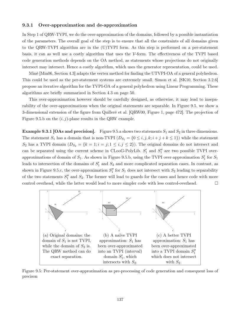
www.dedoimedo.com all rights reserved
9.3.1 Over-approximation and de-approximation
In Step 1 of QRW-TVPI, we do the over-approximation of the domains, followed by a possible instantiationof the parameters. The overall goal of the step is to ensure that all the constraints of all domains givento the QRW-TVPI algorithm are in the (U)TVPI form. As this step is performed on a per-statementbasis, it can as well use a costly algorithm that uses the V-form. The effectiveness of the TVPI basedcode generation methods depends on the OA method, as statements whose projections do not originallyintersect may intersect. Hence a costly algorithm, which uses the generator representation, could be used.
Miné [Min06, Section 4.3] adapts the vertex method for finding the UTVPI-OA of a general polyhedron.This could be used as the per-statement systems are extremely small. Simon et al. [SK10, Section 3.2.6]propose an iterative algorithm for the TVPI-OA of a general polyhedron using Linear Programming. Thesealgorithms are briefly summarized in Section 4.3 on page 50.
This over-approximation however should be carefully designed, as otherwise, it may lead to insepa-rability of the over-approximations when the original statements are separable. In Figure 9.5, we show a3-dimensional extension of the figure from Quilleré et al. [QRW00, Figure 1, page 472]. The projection ofFigure 9.5.b on the (i, j)-plane results in the QRW example.
Example 9.3.1 [OAs and precision]. Figure 9.5.a shows two statements S1 and S2 in three dimensions.The statement S1 has a domain that is non-TVPI (DS1 = {0 ≤ i, j, k; i+ j + k ≤ 1}) while the statementS2 has a TVPI domain (DS2 = {k = 1; i = j; 1 ≤ i, j ≤ 2}). The original domains do not intersect andcan be separated using the current scheme in CLooG-PolyLib. S′1 and S′′1 are two possible TVPI over-approximations of domain of S1. As shown in Figure 9.5.b, using the TVPI over-approximation S′1 for S1leads to intersection of the domains of S′1 and S2 and more complicated separation cases. In contrast, asshown in Figure 9.5.c, the over-approximation S′′1 for S1 does not intersect with S2 leading to separabilityof the two statements S′′1 and S2. The former will lead to guards for the cases and hence code with morecontrol overhead, while the latter would lead to more simpler code with less control-overhead. �
S2
S1
i
j
k
S1’
i
j
k
S2
S1’’
i
j
k
(a) Original domains: thedomain of S1 is not TVPI,while the domain of S2 is.The QRW method can do
exact separation.
(b) A naïve TVPIapproximation: S1 hasbeen over-approximatedinto an TVPI (interval)
domain S′1, whichintersects with S2.
(c) A better TVPIapproximation: S1 hasbeen over-approximatedinto a TVPI domain S′′1which does not intersect
with S2.
Figure 9.5: Per-statement over-approximation as pre-processing of code generation and consequent loss ofprecison
137
www.dedoimedo.com all rights reserved
Loss of precision by OA. As illustrated in Figure 9.5.b, the OA leads to possible control overhead inthe TVPI code generation scheme. Even when the original domains are disjoint, the over-approximationsand their projections can intersect with each other: This is because S1 ∩S2 = φ; OA(S1)∩OA(S2) = φ.
De-approximation. Step 4 of QRW-TVPI is the de-approximation step and is the conjugation of Step 1.It is similar to the post-processing of Omega, or to the backtracking and pattern-matching phase in CLooG.
9.3.2 Preprocessing and variations of QRW algorithm
In Step 2 of QRW-TVPI, we preprocess the domains. Then Step 3 with a small variation of the QRWalgorithm, sketched in Section 9.1.1, is applied. These variations are different for the two algorithms thatwe introduce in this section.
Preprocessing. Each of the algorithms in the QRW-TVPI schema, namely QRW-TVPI1 and QRW-TVPI2, need some preprocessing similar to Hochbaum-Naor’s, which is finding the generators of all theplanar projections. Alternatively, each of the per-statement TVPI domains could be subjected to closurein their graph theoretical representation. These steps reduce the overall complexity since the algorithmswe introduce are based on utmost pair-wise planar projections.
The variations of QRW algorithm are based on the observation that in steps 1–3 of the QRW algorithm,the d-dimensional projections are polyhedral objects in the separation algorithms. These operations canbe done with guaranteed polynomial time on TVPI polyhedra. At dth step of recursion of the originalQRW algorithm, the separation is using the d-dimensions projections of each of the domains. So, thespecializations depend on the following key observation:
Lemma 9.3.2 [Sub-dimensional projections for scanning]. Assume that the scanning order ofthe dimensions in the QRW algorithm is x1, x2, . . . , xd, with x1 being the first dimension that has beenscanned, and xd being the current dimension being scanned (d ≥ 2). Any separation scheme which looks atthe projection of the current d-dimensional domain on only some of the dimensions from {x1, x2, . . . , xd}is valid as long as the (current) dth-dimension (xd) is also being considered.
The above lemma means that a separation of the domains which looks at only the dth dimensional1-dimensional objects (which are interval ranges) is valid. So is the separation of domains which looks atthe 2-dimensional projections, like the ones on xd−1 × xd or x1 × xd planes. Sub-dimensional scheme forthe dth dimension that looks at only the projection on xd−2 × xd−1 plane however, is not valid.
This observation leads to two variations of the QRW-TVPI scheme: QRW-TVPI1 which uses a per-dimensional projection and separation method, and QRW-TVPI2 which uses a planar projection andseparation scheme36.
36Since both methods rely heavily on the Fourier-Motzkin of Hochbaum-Naor, they can alternatively be called FM-TVPI1and FM-TVPI2, but for the fact that they do a separation and sorting after projection, similar to the QRW algorithm.
138
www.dedoimedo.com all rights reserved
QRW-TVPI1: a per-dimension separation. In this variation, the separation of the polyhedra inStep 3 of QRW is on a per-dimensional basis, using only the dth dimension. Consequently, in Step 2 of thismethod, the projection is found on the dth dimension only. The main intuition for this method is that foreach domain of each statement, all the dimensions other than dimension d can be eliminated (projectedaway) in guaranteed polynomial time using Hochbaum and Naor’s Fourier-Motzkin elimination method.The correctness of this method is clear from the above Lemma 9.3.2. The polynomiality of this method isfrom the polynomiality of Hochbaum-Naor’s algorithm in Lemma 9.2.3. We discuss this method and itslimitations in Section 9.4
QRW-TVPI2: closure based planar separations. In this variation, the separation of the polyhedrain Step 3 of QRW is on a planar basis. Since choosing the dth dimension xd is mandatory, we can use theplanar projection on the xi × xd plane (for d ≥ 2 and for any i such that 1 ≤ i ≤ d− 1). The key designissue is which i is to be chosen, among the d− 1 possible choices. A possible heuristic is to fix i = d− 1,but another possible alternative is to generate code for all the d− 1 planes {xi × xd | 1 ≤ i ≤ d− 1}, andto choose the best of the projections among different i’s according to a metric. Again, the correctness ofthis variation is clear from Lemma 9.3.2. The polynomiality of this method is from Lemmas 9.2.3–5. Wediscuss this method and its limitations in Section 9.5.
9.4 QRW-TVPI1: a Per-dimension Separation Method
In this section, we discuss the QRW-TVPI1 algorithm, its strengths and weaknesses. In Section 9.4.1, westudy the QRW specialization for TVPI polyedra, with an example. We study its complexity and othermetrics and some limitations in Section 9.4.2.
Preprocessing. As algorithm QRW-TVPI1 just involves finding the dth dimensional projection of TVPIpolyhedra, the preprocessing involves finding the TVPI approximations of each per-statement domains,followed by possible instantiations. The algorithm needs only the 1-dimensional ranges of each statementon each dimension.
9.4.1 QRW-TVPI1: Algorithm, details and example
The algorithm QRW-TVPI1 is given in Figure 9.6. It is nothing but a simple per-dimension specializationof QRW algorithm. Due to the similarity with the latter, we highlight the differences with the QRWalgorithm sketched in Section 9.1.1.
Details. Steps 1, 4–6 are identical to the QRW algorithm. In Step 2, the domain TVPI polyhedra isprojected on dimension xd, for which, the Fourier-Motzkin of Hochbaum-Naor’s algorithm can be used. InStep 3, these projections are separated into disjoint polyhedra. Since these projections are linear intervalranges, a simple sort based scheme can be used, which also simplifies Step 4.
139
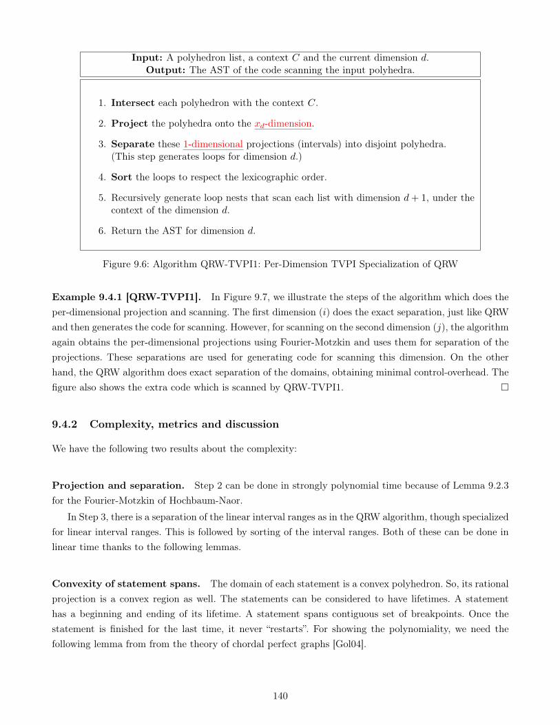
www.dedoimedo.com all rights reserved
Input: A polyhedron list, a context C and the current dimension d.Output: The AST of the code scanning the input polyhedra.
1. Intersect each polyhedron with the context C.
2. Project the polyhedra onto the xd-dimension.
3. Separate these 1-dimensional projections (intervals) into disjoint polyhedra.(This step generates loops for dimension d.)
4. Sort the loops to respect the lexicographic order.
5. Recursively generate loop nests that scan each list with dimension d+ 1, under thecontext of the dimension d.
6. Return the AST for dimension d.
Figure 9.6: Algorithm QRW-TVPI1: Per-Dimension TVPI Specialization of QRW
Example 9.4.1 [QRW-TVPI1]. In Figure 9.7, we illustrate the steps of the algorithm which does theper-dimensional projection and scanning. The first dimension (i) does the exact separation, just like QRWand then generates the code for scanning. However, for scanning on the second dimension (j), the algorithmagain obtains the per-dimensional projections using Fourier-Motzkin and uses them for separation of theprojections. These separations are used for generating code for scanning this dimension. On the otherhand, the QRW algorithm does exact separation of the domains, obtaining minimal control-overhead. Thefigure also shows the extra code which is scanned by QRW-TVPI1. �
9.4.2 Complexity, metrics and discussion
We have the following two results about the complexity:
Projection and separation. Step 2 can be done in strongly polynomial time because of Lemma 9.2.3for the Fourier-Motzkin of Hochbaum-Naor.
In Step 3, there is a separation of the linear interval ranges as in the QRW algorithm, though specializedfor linear interval ranges. This is followed by sorting of the interval ranges. Both of these can be done inlinear time thanks to the following lemmas.
Convexity of statement spans. The domain of each statement is a convex polyhedron. So, its rationalprojection is a convex region as well. The statements can be considered to have lifetimes. A statementhas a beginning and ending of its lifetime. A statement spans contiguous set of breakpoints. Once thestatement is finished for the last time, it never “restarts”. For showing the polynomiality, we need thefollowing lemma from from the theory of chordal perfect graphs [Gol04].
140

www.dedoimedo.com all rights reserved
j
S2
S1
i
j
S2
S1
i
j
S2
S1
i
(a) Original domains tobe scanned
(b) Projection andseparation on the first
dimension
(c) Projection andseparation on the second
dimension
Figure 9.7: QRW-TVPI1: per-dimension separation and code generation for two statements on a planarpolyhedral domain. Also shown are projections of the two statements on the two axes which enable thecode generation.
Lemma 9.4.2 [Statement Elimination Order of Statement]. The statement endings form a linearPerfect Elimination Order (PEO).
The above is a straightforward result from the convexity of the original domains. The above resultmeans that a Lexicographic Breadth First Search (LexBFS) on the statement endings can be done as assuggested by Rose, Leuker and Tarjan [RTL76]. This means that the sorting can be done in linear time,where the ranges are iterated upon by maintaing an annotated list of statement ranges. A statement entersthis list at the beginning of its lifetime and gets removed at its last occurrance.
Lemma 9.4.3 is a consequence from the above results.
Lemma 9.4.3 Projection, separation and sorting in QRW-TVPI1 can be done in polynomial time. HenceQRW-TVPI1 does code generation in polynomial time.
We show a limitation of the code generation method in the following example:
Example 9.4.4 [A hierarchy of precisions]. The example in Figure 9.8 shows that the QRW-TVPI1can help in generating code which is more powerful than one generated by a simple bounding box, but lesspowerful than Omega’s CodeGen, with all of them being less powerful than the QRW’s scheme in CLooG.�
9.5 QRW-TVPI2: Closure Based Planar Separations
In this section, we extend the per-dimension variation studied in the previous section to introduce planarvariations. In Section 9.5.1, we study the QRW specialization for planar polyedra, and illustrate it withan example. Then, we study its complexity, other metrics and its limitations, and list open questions inSection 9.5.2.
141
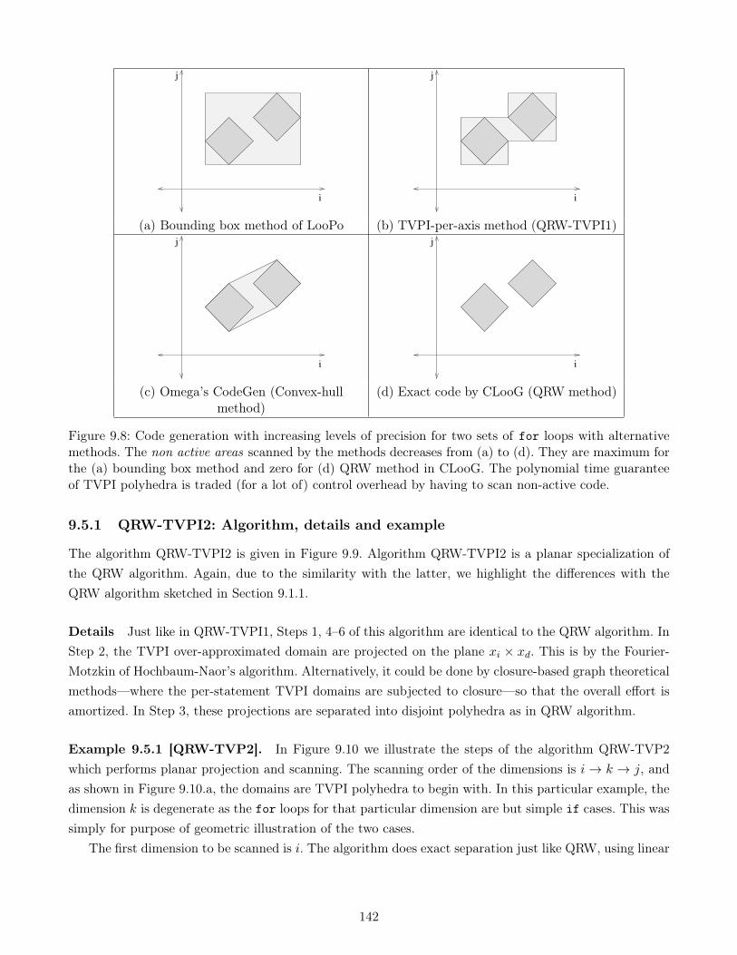
www.dedoimedo.com all rights reserved
i
j
i
j
(a) Bounding box method of LooPo (b) TVPI-per-axis method (QRW-TVPI1)
i
j
i
j
(c) Omega’s CodeGen (Convex-hullmethod)
(d) Exact code by CLooG (QRW method)
Figure 9.8: Code generation with increasing levels of precision for two sets of for loops with alternativemethods. The non active areas scanned by the methods decreases from (a) to (d). They are maximum forthe (a) bounding box method and zero for (d) QRW method in CLooG. The polynomial time guaranteeof TVPI polyhedra is traded (for a lot of) control overhead by having to scan non-active code.
9.5.1 QRW-TVPI2: Algorithm, details and example
The algorithm QRW-TVPI2 is given in Figure 9.9. Algorithm QRW-TVPI2 is a planar specialization ofthe QRW algorithm. Again, due to the similarity with the latter, we highlight the differences with theQRW algorithm sketched in Section 9.1.1.
Details Just like in QRW-TVPI1, Steps 1, 4–6 of this algorithm are identical to the QRW algorithm. InStep 2, the TVPI over-approximated domain are projected on the plane xi × xd. This is by the Fourier-Motzkin of Hochbaum-Naor’s algorithm. Alternatively, it could be done by closure-based graph theoreticalmethods—where the per-statement TVPI domains are subjected to closure—so that the overall effort isamortized. In Step 3, these projections are separated into disjoint polyhedra as in QRW algorithm.
Example 9.5.1 [QRW-TVP2]. In Figure 9.10 we illustrate the steps of the algorithm QRW-TVP2which performs planar projection and scanning. The scanning order of the dimensions is i→ k → j, andas shown in Figure 9.10.a, the domains are TVPI polyhedra to begin with. In this particular example, thedimension k is degenerate as the for loops for that particular dimension are but simple if cases. This wassimply for purpose of geometric illustration of the two cases.
The first dimension to be scanned is i. The algorithm does exact separation just like QRW, using linear
142
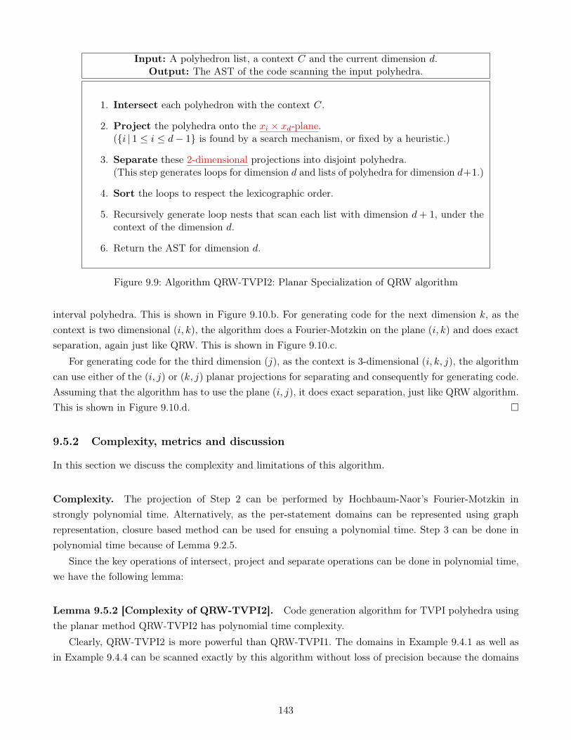
www.dedoimedo.com all rights reserved
Input: A polyhedron list, a context C and the current dimension d.Output: The AST of the code scanning the input polyhedra.
1. Intersect each polyhedron with the context C.
2. Project the polyhedra onto the xi × xd-plane.({i | 1 ≤ i ≤ d− 1} is found by a search mechanism, or fixed by a heuristic.)
3. Separate these 2-dimensional projections into disjoint polyhedra.(This step generates loops for dimension d and lists of polyhedra for dimension d+1.)
4. Sort the loops to respect the lexicographic order.
5. Recursively generate loop nests that scan each list with dimension d+ 1, under thecontext of the dimension d.
6. Return the AST for dimension d.
Figure 9.9: Algorithm QRW-TVPI2: Planar Specialization of QRW algorithm
interval polyhedra. This is shown in Figure 9.10.b. For generating code for the next dimension k, as thecontext is two dimensional (i, k), the algorithm does a Fourier-Motzkin on the plane (i, k) and does exactseparation, again just like QRW. This is shown in Figure 9.10.c.
For generating code for the third dimension (j), as the context is 3-dimensional (i, k, j), the algorithmcan use either of the (i, j) or (k, j) planar projections for separating and consequently for generating code.Assuming that the algorithm has to use the plane (i, j), it does exact separation, just like QRW algorithm.This is shown in Figure 9.10.d. �
9.5.2 Complexity, metrics and discussion
In this section we discuss the complexity and limitations of this algorithm.
Complexity. The projection of Step 2 can be performed by Hochbaum-Naor’s Fourier-Motzkin instrongly polynomial time. Alternatively, as the per-statement domains can be represented using graphrepresentation, closure based method can be used for ensuing a polynomial time. Step 3 can be done inpolynomial time because of Lemma 9.2.5.
Since the key operations of intersect, project and separate operations can be done in polynomial time,we have the following lemma:
Lemma 9.5.2 [Complexity of QRW-TVPI2]. Code generation algorithm for TVPI polyhedra usingthe planar method QRW-TVPI2 has polynomial time complexity.
Clearly, QRW-TVPI2 is more powerful than QRW-TVPI1. The domains in Example 9.4.1 as well asin Example 9.4.4 can be scanned exactly by this algorithm without loss of precision because the domains
143
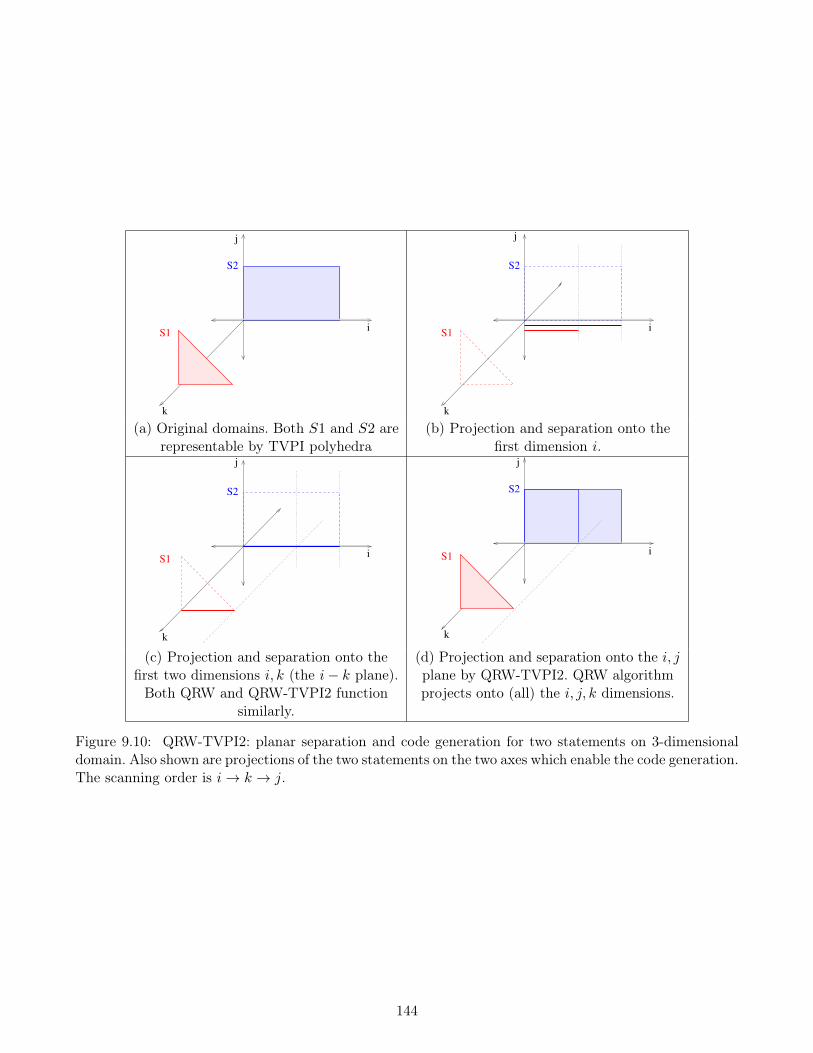
www.dedoimedo.com all rights reserved
S2
k
iS1
j
S2
k
iS1
j
(a) Original domains. Both S1 and S2 arerepresentable by TVPI polyhedra
(b) Projection and separation onto thefirst dimension i.
S2
k
iS1
j
S2
k
iS1
j
(c) Projection and separation onto thefirst two dimensions i, k (the i− k plane).Both QRW and QRW-TVPI2 function
similarly.
(d) Projection and separation onto the i, jplane by QRW-TVPI2. QRW algorithmprojects onto (all) the i, j, k dimensions.
Figure 9.10: QRW-TVPI2: planar separation and code generation for two statements on 3-dimensionaldomain. Also shown are projections of the two statements on the two axes which enable the code generation.The scanning order is i→ k → j.
144
www.dedoimedo.com all rights reserved
there are planar and hence representable by TVPI polyhedra. For 2d-loops, loops with at most two indices,the algorithm works exactly as QRW algorithm. But, for higher dimensional loops, it offers a choice.
Mechanism for selecting xi: In the above QRW-TVPI2 algorithm, for each d ≥ 2, a dimension{i | 1 ≤ i ≤ d− 1} has to be chosen. Among these d− 1 choices, we suggest the following alternatives forselecting xi.
• Search: Since there are d − 1 possible choices, a linear search can be done. The key issue here isdesigning a cost function which can be used as an evaluation metric: namely, which {i| 1 ≤ i ≤ d− 1}ensures that code generated using the xi × xd plane is the best?
• Heuristic: Alternatively choose i to be d − 1 (or even to any predetermined {i| 1 ≤ i ≤ d− 1}),such that code is always generated using the projection on the xi × xd plane. This method hasthe advantage of very simple implementation, though there could be loss of precision when betteralternatives exist. For example, there may exist a {i′ | 1 ≤ i′ ≤ d− 2} such that code generated bythe plane xi′ × xd is much superior to the one generated by the choice of xd−1 × xd.
To show the limitations of the heuristic and the power of the search mechanism, we use Example 9.5.1again.
Example 9.5.1 (contd.) [search vs. heuristic]. In this example, when generating code for the thirddimension j, there exists a choice as to which planar projection to choose for separation: i× j or k× j. Ifthe algorithm QRW-TVPI2 uses the plane k × j, then, the code generated for the dimension j is trivial:it is equivalent to what the less powerful per-dimensional scheme QRW-TVPI1 generates.
Instead, as illustrated in Figure 9.10.d, choosing the planar projection i × j for the same purposeswould mean that the code generated is exact, and equivalent to the one generated by QRW algorithm. �
The above example shows that the heuristic selection of i is limited and can result in a poor choice forcode generation. It also shows that there exists a choice while selecting a planar projection for separatingthe domains. The QRW algorithm does not need to make this choice as it can use the d-dimensionalpolyhedra for separation. By making this choice however, QRW-TVPI2 runs in guaranteed polynomialtime, while being more powerful than QRW-TVPI1.
We leave this sub-section with the following open questions:
Open questions:
• In the search mechanism suggested, what are possible metrics to evaluate the best of the {xi × xd | 1 ≤ i ≤ d− 1}planes?
• Among these d−1 choices, can the metric provide a control in the generated code, similar to CLooG’s-l and -f options?
• Also, for real world examples, how effective are the above alternatives in terms of reduction ofscanning of inactive code?
145
www.dedoimedo.com all rights reserved
• Furthermore, can the separation problem in Step 3 of QRW-TVPI2 be reduced to a graph theoreticalproblem by making a correspondence between the above choices and the code generated?
9.6 A Summary of Additional Related Work
We summarize additional related work.
Code generation methods and QRW algorithm. An excellent summary of code generation meth-ods is in the encyclopediac reference by Bastoul [Bas11]. The above reference helped in preparation ofSection 9.1.1 on page 128 of this chapter. Quilleré et al’s [QRW00, Bas04a] algorithm (QRW algorithm)whose extension is in Bastoul [Bas04a] and Bastoul [Bas04b, Chapters 6,7]. The algorithm is implementedin the widely used code-generator CLooG with many improvements. CLooG is designed so that the basicimplementation within is independent of the library which supports the necessary polyhedral operations.The focus of this chapter is however on CLooG-PolyLib, which uses the PolyLib library for polyhedraoperations.
Implementation of closure operation. An implementation of the algorithms suggested in this chaptercould use the closure based implementations like TVPI by TVPI-lib [SKH02] or Octagons by Apron [JM09]or PPL [PPL].
Chen’s recent PLDI work. Recently, Chen [Che12] improved CodeGen to CodeGen+. The latter isbased on Omega 2.0 and it appears from the algorithm that it is quite similar to the one by Kelly, Pugh andRosser [KPR95], with the improvements being limited to changes in the post-processing methods alongwith changes in the way control structures in the AST—in particular the if conditionals—are removed bypost processing.
CodeGen, and hence CodeGen+ operate with the philosophy that the input should come with alexicographic ordering of the statements. Such a method is quite different from how CLooG operates,which expects separate inputs for the domains and the scattering functions. This kind of separation givesCLooG more freedom in generating many varieties of code with its many flavors—like its two options-l <depth> and -f <depth>—which allow tuning the amount of control in the generating code, whichOmega based code generators cannot do. This latter reason makes the paper under consideration [Che12]mistate that CLooG could generate incorrect code, while actually CLooG does not need to know about thecorrectness of the generated code: its responsibility solely being limited to respecting the input scatteringfunctions which it does all along.
The implementation of CodeGen+ has also been compared to a version of CLooG. Among the metricsof code compactness (generated code size), code generation time, GCC compile time (of the generatedcode) and code performance, Chen’s implementation reports dramatic improvements over CLooG on thecode size (and consequently, the GCC compile time) and the code generation time metrics. It howeverappears from the numbers in the paper that the improvements of the executed code of CodeGen+ onCLooG are not significant. This is not surprising because the algorithm of QRW which is the main engine
146
www.dedoimedo.com all rights reserved
of CLooG, generates exact code with no redundancy and hence improving on the executed code is notpossible. On the other hand, improving on the complexity of the QRW algorithm is possible because ofthe cost of the algorithms used in it, and it is likely that the significant gains in code generation time ofChen’s implementation are due to the core engine and the above improvements.
In spite of the improvements of Chen’s algorithm over CLooG over running time, it is unlikely thatoffers asymptotic improvements over CLooG. This is because the basic engine of CodeGen+ is potentiallyas costly—if not more costly—as the basic engine of CLooG. It is likely that the Omega 2.0 does efficientpattern matching for common cases as suggested much earlier by Pugh [Pug92]. But, as we pointedout in Chapter 4, these heuristics of Omega need to be augmented with an appropriate over- or under-approximation methods so as to obtain asymptotic improvements.
147

www.dedoimedo.com all rights reserved
9.7 Conclusions, Perspectives and Related Work
In this section, we review the conclusions and contributions of this chapter, as well as discuss someperspectives.
9.7.1 Conclusions and contributions
Conclusions. In this chapter, we showed how the polynomial complexities of TVPI polyhedral operatorscan be exploited to obtain polynomial time complexities for code generation. First, we identified the twosources of exponentialities in QRW algorithm: the separation of abstract polyhedral objects, and thecomplexities associated with the algorithms of the underlying polyhedral operations. Then, we proposeda TVPI code generation scheme which exploits the polynomial properties of TVPI polyhedra. Usingthis scheme, we presented two algorithms–a per-dimensional one, and a planar one–each of which arespecializations of the QRW algorithm and which do the crucial polyhedral operations of projections andseparation in asymptotically polynomial time. The insights for these algorithms are very simple: for TVPIpolyhedra, finding the 2d-projections for each pairs of dimensions, Fourier-Motzkin and hence, the crucialoperations of polyhedral projection and separation can be performed in a guaranteed polynomial time.
Loss of precision. Though guaranteeing a polynomial time complexity, the algorithms presented exhibittwo causes of precision loss. The first source of precision loss is the over-approximation method. This canlead to non-empty intersection of the over-approximated domains OA(S1) ∩ OA(S2) = φ, even when theoriginal domains are disjoint, S1 ∩ S2 = φ. This leads to an increase of code-size, and hence an increase ofcompilation time of the generated code, and an increase of the control overhead and hence execution timethe generated code.
The second source of precision loss is the projection and separation methods. In the per-axis (per-dimension) separation method QRW-TVPI1, the loss of precision can be significant. The planar schemesin QRW-TVPI2 are better. In these latter, the heuristic which uses the xd−1×xd plane for separation is lessprecise than the closure-based search scheme which generates the code for each of the xi× xd planes with{i | 1 ≤ i ≤ d− 1}, and chooses the one with the best code that is generated, with best defined accordingto an appropriately pre-defined metric, like controlling the control-overhead.
Hierarchies of precision. Let us use the symbol ≤ to denote, rather loosely, a gradation of precisionof two sub-polyhedral code-generation algorithms. Informally, it captures the quality of generated codein terms of control overhead, or equivalently the volume of non-active code scanned: A1 ≤ A2 for twoalgorithms A1 and A2 means that A1 has more control overhead, and hence scans more inactive code thanA2. With the above notation, the algorithms introduced fit in the following hierarchy of code generation:
QRW-TVPI1 ≤ QRW-TVPI2Heuristic ≤ QRW-TVPI2Search︸ ︷︷ ︸Polynomial Time
≤ QRW︸ ︷︷ ︸Exponential Time
148

www.dedoimedo.com all rights reserved
In addition to the algorithms listed above, we have the corresponding additional UTVPI specialization ofthe QRW algorithm: QRW-UTVPI1 and QRW-UTVPI2, which use similar ideas and all of which introducethe following hierarchy:
QRW-UTVPI1 ≤ QRW-TVPI1 ≤ QRW-UTVPI2 ≤ QRW-TVPI2
Each algorithm in the above hierarchy is polynomial because of the reduced complexities of projectionand separation.
Contributions. The result in this chapter could be seen either as a new code generation method, or amore precise complexity analysis for CLooG when the domains are (U)TVPI polyhedra. We introducedsome open problem which could be used to make a closer connection between the geometric methods usedin polyhedral code generation, in particular the QRW algorithm and graph theory.
The material in this chapter has not been published anywhere before.
Memory improvements. As for sub-polyhedral scheduling, the memory savings of (U)TVPI polyhedracould be considerable, making the overall system very light on the system. We believe that, as suggestedin Halbwachs et al. [HMG06], many techniques could be used to improve the memory requirement, butbeyond an certain level, asymptotic improvement is not possible and sub-polyhedral methods like ourshave to be used.
9.7.2 Perspectives and discussion
Advantages in using (U)TVPI polyhedra
Improvements over general polyhedra. When compared to general convex polyhedra, the improve-ments in complexities suggested by the TVPI specializations of QRW and its approximations can begauged from the following: for normal polyhedra, obtaining the d-dimensional projections may take ex-ponential time. Given a TVPI-OA of each domain, we can run QRW algorithm, but the d-dimensionalseparation algorithm takes exponential time. So, using (U)TVPI polyhedral over-approximations, alongwith the improvements to the QRW algorithm is one simple way in which the exponential parts can bereduced to polynomial time.
Practical utility and limitations. Alternatively, it also true that the exponentialities mentioned inSection 9.1.2 on page 129 are rarely observed and the running time of CLooG is quite fast. In fact, thishas been reported many times in the polyhedral literature—for example by Wilde [Wil93] in PolyLib, An-court [Cor91] for PIPS, Pugh [Pug92] for Omega—that the exponentialies due to the polyhedral operations(“second exponentiality” in Section 9.1.2) in are seldom observed in practical inputs. Even the QRW papersuggests similar reasons for using PolyLib with its first implementation: that it scales well because thenumber of dimensions is small. Furthermore, CLooG-PolyLib has been a successful code-generator. But,this chapter is about improvement of theoretical complexity using better guarantees offered by (U)TVPI
149
www.dedoimedo.com all rights reserved
polyhedra. Beyond the above limitations, the new methods proposed also do need a backtrack or un-approximation phase in which the guards have to be removed. This process may be costly and could bedifficult to implement as well.
Statistical verification. One of our assumptions is that a good portion of constraints from real-worldbenchmarks are TVPI to begin with. A thorough experimental verification from CLooG benchmarks, aswell as, from Omega benchmarks could be done; such a validation could help formalize many folklorehunches, like our ealier statistical study in Section 7.2. Also helpful in this aspect are the statistics re-ferring to (U)TVPI domains in Maydan et al. [MHL91] and the subsequent comments by Pugh [Pug92].Furthermore, looking at how Omega handles UTVPI domains may be helpful.
Though in this chapter we focussed mainly on TVPI polyhedra, UTVPI specialization would havesome additional advantages:
QRW’s modulo operations and UTVPI polyhedra. It is known [Bas04b, Bas12] that the QRWalgorithm is limited by the costly modular operations it generates. In the previous chapter, in Section 8.8on page 123, we suggest that obtaining a UTVPI-UA of the per-dependence Farkas polyhedron which hasinteger homogenizing dimension values would result in the overall Farkas polyhedon to have just integervertices because of Total-Unimodularity. The same reason applies to removing the modularities associatedwith QRW algorithm. These can be removed by obtaining UTVPI over-approximations and using theTotally Unimodularity and integer vertices associated with UTVPI sub-polyhedral over-approximations.A similar method has originally been hinted by Bastoul and Griebl [Bas04b, Section 6.2.2, page 134] whosuggest restricting the transformation coefficients to {0,±1} so that modulos are not generated. UsingUTVPI schedules has the advantage of integer-vertices along with the additional advantage of improvedguarantee of polynomial time complexity.
Dealing with non-TVPI constraints
The non-TVPI constraints have to be over-approximated on a per-statement basis initially. After theQRW-TVPI code generation, they have to be de-approximated.
Over-approximations. For general convex polyhedra, the methods suggested in this chapter needan over-approximation algorithm. The effectiveness of the TVPI based code generation methods de-pends on the OA method as domains with non-intersecting original projections may intersect whenover-approximated. Hence a costly algorithm which uses the generator representation could be used.Miné [Min06, Section 4.3] adapts the vertex method for finding the UTVPI-OA of a general polyhedron.This could be used because the per-statement domain systems are extremely small. Simon et al. [SK10,Section 3.2.6] propose an iterative algorithm for the TVPI-OA of a general polyhedron using LinearProgramming. We have summarized these algorithms briefly in Section 4.3 on page 50. But, this over-approximation should be carefully designed as it could decrease the quality of the generated code byintroducing additional guards, i.e., control overhead.
150
www.dedoimedo.com all rights reserved
Limitation for un-approximable domains. Similar to the polyhedra in Section 6.7.4 on page 80 forwhich there exist only trivial under-approximations, there may be real world domains—for examples, oneswith non-trivial lineality space—that cannot be over-approximated by a TVPI domain. For these kindsof degenerated cases, the usual QRW method can be followed. Or, techniques which involve splitting ofthese domains along with an under-approximation method could be used.
De-approximation. Though we have not discussed the implications of the over-approximation processin this chapter, in particular the de-approximation (un-approximation) algorithm, we consider its designand practical implications quite crucial for the success of the schemes suggested here. This phase could besimilar to the methods in CLooG or CodeGen of Omega. We however leave its discussion for future work.
Code generation and (U)TVPI as abstract domain
The understanding that operators on (U)TVPI sub-polyhedral domains have excellent complexity measuresled to their use in static analysis with wide ranging success. The very same reason led to the proposal of(U)TVPI sub-polyhedral scheduling and (U)TVPI sub-polyhedral code-generation as a means to reducethe complextiy of the most prominent loop parallelization applications of scheduling and code generation.But, sub-polyhedral scheduling, which is the main contribution of this thesis and covered in the earlierchapters, does not use the abstract domain properties of sub-polyhedra at all, instead directly relyingon the complexity of under-approximation algorithms, and the complexity of solution of (U)TVPI sub-polyhedral linear programs. In contrast, sub-polyhedral code generation proposed in this chapter, by itsreliance of image, projection, intersection, and union operations, uses (U)TVPI sub-polyhedra more as anabstract domain.
151

www.dedoimedo.com all rights reserved
152

Chapter 10
Conclusions and Perspectives
It is well true that automatic loop parallelization is the most powerful optimization designed as part ofcompiler optimizations. Though it is surprising that it took a couple of decades for main stream compilercommunity to accept the polyhedral compilation framework, it has now become the acceptable norm forcompilation of loop programs. Examples are the implementations of variations of the Forward Communica-tions Only framework of PLuTo implemented in the various polyhedral compilers like IBM-XL, ReservoirLabs R-Stream, GCC-GRAPHITE and LLVM/Polly. A direct consequence of the above success, is thatit is likely that the size of the input programs to the polyhedral compiler would increase, and hence itbecomes more pertinent for the polyhedral community to solve the scalability challenge.
Summary. In this thesis we contributed to some of the challenges of scalability in polyhedral compila-tion by introducing algorithmic analysis and complexity based approximation based methods to use(Unit-)Two-Variables-Per-Inequality sub-polyhedra. More particularly, we proposed sub-polyhedral com-pilation using (Unit-)Two-Variables-Per-Inequality as a means of obviating the scalability challenges inpolyhedral compilation. The methods in this thesis should only be seen only as the initial steps in solvingthe hard to solve scalability problem.
Contributions
The following are the contributions of this thesis.
Scalability challenges and sub-polyhedral compilation
The first contribution of this thesis is the complexity driven analysis of the different modules of thepolyhedral compiler. In particular with the success of various polyhedral compilers one is directly leadto ask the obvious questions: “Will they scale for large inputs? If not, what are the techniques to makethem scale?”. For answering the above questions, using theoretical and empirical analysis of the variousmodules of polyhedral compilation, we showed that current methods that use general convex polyhedra aspolyhedral abstractions (for dependences, domains and transformations) do not scale. Trying to integratethe polyhedral compiler as a phase in any compiler would mean solving the scalability challenge.
153

www.dedoimedo.com all rights reserved
The suggestion of sub-polyhedral compilation is but a natural progression from the above answers.We suggested that sub-polyhedra could be used in affine scheduling and polyhedral code generation sothat practically scalable and asymptotially better algorithms could be designed. The key concepts in ourapproaches are algorithmic approaches and complexity driven approximations.
Affine scheduling using (U)TVPI sub-polyhedra
In understanding the various options available options for use in scalability in sub-polyhedra, (Unit-)Two-variables-Per-Inequality Sub-Polyhedra or (U)TVPI sub-polyhedra come at the forefront. We studied inChapter 3 that these latter flavors of sub-polyhedra have been used both by the theoretical (algorithmic)community as well as by the static analysis community.
The advantages with these varieties of sub-polyhedra are that they admit graph theoretic algorithmsfor solving linear optimization problems when the input problem formulations are of restricted (U)TVPIform. More particularly, TVPI constraints can be solved using (generalized) min-cost flow algorithms, whileUTVPI constraints can be solved using Bellman-Ford and Johnson’s algorithms. For the same reasons,the static analysis community has been successfully using (U)TVPI sub-polyhedra as abstract domainsfor abstract interpretation problems.
In Chapter 4, we introduced the concept of sub-polyhedral scheduling using Unit-Two-Variables-Per-Inequality polyhedra. This method solves the scalability problem from within the affine scheduling frame-work by using the concept of sub-polyhedral Under-Approximations (UA) and can be applied in two mainways: UAs of the per-dependence Farkas polyhedra to result in an intersection of these individual approx-imations, and UA of the overall Farkas polyhedron which can be used on an offline/online basis.
Polynomial time algorithms for (U)TVPI approximation
The above sub-polyhedral affine scheduling methods also do need appproximation algorithms with low com-plexity. We proposed worst-case polynomial time algorithms to compute (U)TVPI under-approximationsbeginning from a general convex polyhedron.
For doing the above, in Chapter 5 we developed a simple polarity based framework that can be usedto design approximation algorithms. In Chapter 6, we used the above framework to design simple andasymptotically worst-case polynomial time algorithms that take a general convex polyhedron and under-approximate it into (U)TVPI polyhedra. One of the algorithms finds the UA in a heuristic fashion, whilethe other by framing a higher dimensional linear program. To stay within polynomial time, care wastaken to linearize the under-approximation model, avoiding the exponential vertex and ray constructionassociated with the Chernikova algorithm. We explored different heuristics relying on bounded-size linearprograms to trade complexity for feasibility.
In Section 6.7.5, we also suggested a small variation of the above framework to obtain integer polyhedralapproximations of rational polyhedra, by using ILP formulations of small size. This method brings theconcept of Total-Unimodularity from the mathematical programming community to be used in polyhedralcompilation.
154

www.dedoimedo.com all rights reserved
Experimental evaluation of our techniques
In Chapter 7, we showed initial results of the above approximations when integrated into the PLuTopolyhedral compiler. We began with a study of the polyhedral characteristics of the benchmarks in Poly-Bench 2.0.
This was followed by studying the experimental results of preservation of feasibility of the under-approximations using various algorithms that we proposed. We showed that the feasibility is preservedfor 10 out of 16 number of benchmarks from PolyBench 2.0. We also studied the scalability experiments,where we compared the running times of solving the original system using traditional simplex vs. solvingthe under-approximated system using Bellman-Ford. We showed an asymptotic improvement in scalability,answering positively the scalability challenge. We also showed that a preliminary integration of the aboveUA polyhedra into PLuTo yields code for a few PolyBench 2.0 benchmark cases that does not suffersignificant increase in execution time.
Applications to various loop transformation problems
In Chapter 8, we showed an illustration of the power of our approximation scheme by applying it forimportant loop transformation problems. We introduced a hierarchy of loop transformation problems re-garding the type of transformations they can affect: 1d transformations, more general multi-dimensional(affine) transformations which encode multitudes of useful transformations, and specific tailor-made multi-dimensional transformations. We also introduced a gradation of these problems regarding their computa-tional complexity: strongly-polynomial time, weakly polynomial time and hence admitting LP formula-tions, or NP-Complete and hence admitting ILP or MILP formulations. Each of the above problems canadmit polynomial time under-approximation algorithms, which can be used for both understanding theproblem complexity, as well as for obtaining algorithmic solutions.
Unique to the above under-approximation based solutions is the use of Total Unimodularity resultin approximations in scheduling which was introduced in Section 6.7.5. By this method, an integerpolyhedral under-approximation is obtained by solving an ILP formulation on a per-dependence basis.When the per-dependence under-approximations are UTVPI approximations, the resultant overall under-approximation—which is the intersection of all these individual under-approximations—will result in asystem for which LP formulation will automatically result in an integer optimal solution as well, in caseswhen the under-approximation preserves the feasibility.
Sub-polyhedral code generation
In Chapter 9, we proposed a sub-polyhedral code generation using (U)TVPI polyhedra. For doing the above,we began with a complexity oriented theoretical study of the of Quilleré, Rajopadhye and Wilde [QRW00](QRW) algorithm, which is considered to be the most successesful of the polyhedral code generationschemes because of their implementation in the widely used code generator CLooG [Bas04a]. We identifiedthat the two causes of exponentiality that can cause scalability challenges in the code generation can bereduced to polynomial time using (U)TVPI polyhedra.
155

www.dedoimedo.com all rights reserved
Using simple concepts like (U)TVPI sub-polyhedral over-approximations of per-statement domainsand use of sub-dimensional projections for scanning, we introduced a scheme to create specializations ofthe QRW algorithm. Using the above scheme, we proposed two new algorithms: a per-dimensional onewhich does the separation of the domains on a per-dimensional basis; and a planar one which does theseparation by using projections on planar polyhedra.
Both of these algorithms can solve the polyhedral code generation in guaranteed worst-case polynomialtime.
Perspectives
Though we have raised many questions in the course of this thesis and provided only a few answers, wehope that the methods suggested in this thesis are interesting enough to be starting points for furtherresearch. The following are some broad directions in which the methods suggested in this thesis could beextended.
Program theoretic approach
One primary focus of this thesis is on the algorithmic (complexity theoretic) advantages that (U)TVPIsub-polyhedra offers, and designing the ways in which these can exploited in polyhedral compilation. Sucha kind of approach could be further strengthened by complementing it with a study of program theoretic(and transformational) approach as well. In this, a study of the kind of programs that are best suitedfor (U)TVPI sub-polyhedral compilation could be done. Or, a classification of transformations could bemade which are easily possible by solving the inexpensive graph theoretic algorithms of min-cost flow orBellman-Ford algorithms in the dual space. However, this understanding could be quite different from theapproach of Balasundaram and Kennedy [BK89], in the sense that the work in the new direction is still onthe Farkas polyhedron; and our suggested method still does an under-approximation of this latter, whilepreserving specific interesting program transformations in the primal.
Examples where such under-approximations could help are the the multi-dimensional shifting by Darteand Huard [DH00a] and the array contraction results by Darte and Huard [DH05]. Though both of thesetransformations are interesting, the NP-Completeness of the associated problems could hinder their prac-tical application. However, approximations which preserve interesting transformations from these formula-tions would be of use to the community. Equally important is the case of the fusion heuristics by Pouchetet al. [PBB+11] which could also benefit from (U)TVPI approximations.
Feasibility preservation
Related to the above direction is the problem of preservation of feasibility of intersections of under-approximations. Indeed, the difficult problem in the methods given in Chapter 6 is the lack of a scalableway to reliably preserve the non-emptiness of the under-approximation when the original polyhedron isnon-empty. The one-shot linear programming method offers this guarantee, but is clearly not in stronglypolynomial time and there could be limitations in applying it over multiple dependences. We know that
156
www.dedoimedo.com all rights reserved
this problem of finding a feasible UA by paying a small cost is difficult, because a strongly polynomialmethod with this guarantee could directly lead to a solution of finding strongly polynomial feasibility testfor general polyhedra.
In Chapter 8, we have provided some hints for preserving the feasibility in the presence of multiple-dependences arising from different loop transformation applications; namely by preserving the unit-schedule(canonical schedule) for each dependence and collecting the overall under-approximations, clustering theconstraints and dependences so that one-shot method can be applied to the indvidual clusters, and evenclustering of input sections of programs. Still, this problem largely remains unsolved and there needs tobe further theoretical study as well as practical work in each of these directions.
Such a study is bound to be complicated for an affine formulation like Forward Communications Only.In this latter transformation as formulated by a scheduler like PLuTo, the LP problems are on a level-by-level basis searching for permutable hyperplanes, and with the inherent limitation that there is noguarantee of preservation of feasibility in the original (un-approximated) Farkas constraint system. Forsuch input systems, the study of preservation of feasibility of the under-approximated systems (as in theYY or YN cases), along with the consequent impact on the amount of parallelism lost is indeed bound tobe challenging.
Experiments and impact on the transformed code
Another limitation of the methods suggested in this thesis is the fact that we have been successful ingenerating code only for a few cases from PolyBench as part of experiments. Though we have discussedthis issue at length in the conclusions section of Chapter 7, this needs more work in the sense of acomplete evaluation of the performance impact of the approximation on all PolyBench benchmarks using anapproximated objective function compatible with the algorithm which is used for solving the approximatedsystems. The latter aspect which is measured in terms of the running times of the output generated code,is the true measure of the loss of performance and hence another answer to the precision vs. cost tradeoff.
Future experiments should also include fast duplicate elimination schemes and their impact on therunning times, and a complementary study of the memory complexity of the original as well as the under-approximated systems, known to be overwhelmingly in our favor.
Memory complexity reduction
This latter aspect of memory reduction of the polyhedral compiler is, at least sometimes arguably moreimportant than the time-complexity reduction, which we have primarily focused in this thesis. Though itis well understood that both polyhedral scheduling and polyhedral code-generation are memory intensiveoperations, little can be done with the current algorithms themselves, because of their inherent limitations.
The polyhedral scheduling inherently reduces to constructing a large (quadratic) size simplex tableau,which can be quite costly in practice. Also, polyhedral code-generation of the QRW algorithm is wellknown to be highly memory intensive, primarily because of the need for dual representations of polyhedraand the way existing libraries like PolyLib [Wil93] implement these. (CLooG-PolyLib [Bas04a, Bas04b]is known to face these memory scalability problems.) While both these operations can be prohibitively
157
www.dedoimedo.com all rights reserved
expensive even for a conventional compiler, they will be more so for a compiler like LLVM/Polly, and stepsshould be taken to reduce them. In contrast, either of the (U)TVPI sub-polyhedra can be encoded in linearmemory and hence are extremely light on the memory requirements—which has been practically observedin the course of experiments in this thesis—and this will be quite useful for any variety of compilationsystem.
Sub-polyhedral code generation
The particular aspect of raising more questions than answering them is true more so for our work onpolyhedral code generation in Chapter 9, where we have relied on the complexities of the (U)TVPI sub-polyhedra to design polynomial time code generation schemes. This result could be improved in severalways.
One important subroutine in the design of sub-polyhedral code-generation schemes is the method todeal with non-(U)TVPI constraints and domains. The method we have focused in the chapter is to over-approximate the per-statement domains by using existing algorithms, followed by a de-approximationphase. Both of these phases need to be designed carefully because of the possible impact they have on therunning time, as well as the quality of code-generated. We have suggested some options for both of thesephases in the above chapter. Either of these operations could be based on the generator representationbecause of the small cost of the per-statement domains, and hence designing them should be done with anemphasis more on improving precision in the form of generated code, and not with reducing the runningtime of the algorithms.
Equally important is the study of the impact of the precision vs. cost tradeoff on practical inputs. Useof (U)TVPI polyhedra is bound to result in loss of precision whch reflects in the form of more control-overhead in the generated code, but it remains to be seen how it effects practically. Trying to reduce thecontrol-overhead using heuristics methods like Omega does for CodeGen [KPR95] is an option, but it islikely that such method would be engineering intensive, and more importantly lose the simplicity of theQRW algorithm.
There is also a need for designing a graph theoretic algorithm to choose the proper plane with anappropriate cost function in case of our planar algorithm QRW-TVPI2. Since the algorithm in effect hasto search for a plane (among the possible d − 1 alternatives) to project the domains such that a propercost function is minimized, its design could also involve a tunable parameter by which one can control theprecison of the generated code.
Further, there is need for representative examples, whether real or artificial, which clearly illustrate theexponentialities of the QRW algorithm as implemented in CLooG-PolyLib [Bas04a, Bas04b]. Beginningwith such examples would clearly illustrate the improvements in the running time as well as showing theloss of precision by use of our specializations.
We believe each of these are challenging aspects to be solved in sub-polyhedral code-generaton toachieve asymptotically better code-generation schemes which are practically useful as well.
*****
158
www.dedoimedo.com all rights reserved
A Chronological Order
The following is a chronological order of the contributions in this thesis:
• ... 2009-2010: Wide success of PLuTo algorithm and its implementation. Scalability challenges inIBM compiler and Reservoir Labs R-Stream compiler. Integration of a polyhedral compiler in theGCC’s GRAPHITE.
• Early and mid 2010: Study of use of (U)TVPI polyhedra by theoretical community and sub-polyhedraby the static analysis community.
• Late 2010: Proposal of sub-polyhedral affine scheduling using under-approximations.
• IMPACT-11 [UC11] acceptance and feedback.
• Early 2011: Scalability complexity study with unrolled examples.
• Mid 2011: Design of (U)TVPI Under-approximation algorithms.
• Late 2011: Implementation in PLuTo polyhedral compiler.
• IMPACT-12 [UC12] acceptance and feedback.
• Early and middle 2012: Implementation, asymptotic improvement by using UTVPI polyhedra.Various applications, Total-Unimodularity result.
• POPL-13 [UC13] acceptance and feedback.
• Late 2012: Proposal of sub-polyhedral code generation.
159
www.dedoimedo.com all rights reserved
A Personal Bibliography
International Conferences/Workshops
• (with Albert Cohen): Sub-Polyhedral Scheduling Using (Unit-)Two-Variable-Per-Inequality Polyhe-dra, published in 40th ACM SIGPLAN-SIGACT Symposium on Principles of Programming Lan-guages (ACM-POPL-2013), Rome, Italy, January 2013.
• (with Albert Cohen): A Case for Strongly Polynomial Time Sub-Polyhedral Scheduling Using Two-Variable-Per-Inequality Polyhedra, published in 2nd International Workshop on Polyhedral Compi-lation Techniques (IMPACT-2012), in conjunction with HiPEAC’12, Paris, France, April 2012.
• (with Albert Cohen): Potential and Challenges of Two-Variable-Per-Inequality Sub-Polyhedral Com-pilation, published in 1st International Workshop on Polyhedral Compilation Techniques (IMPACT-2011), in conjunction with CGO’11, Chamonix, France, April 2011.
• (with GRAPHITE team): GRAPHITE Two Years After: First Lessons Learned From Real-WorldPolyhedral Compilation, published in 2nd International Workshop on GCC Research Opportunities(GROW’10), Pisa, Italy, January 2010.
• (with L. Renganarayana and S. Rajopadhye): Combined ILP and Register Tiling: Analytical Modeland Optimization Framework, published in The 18th International Workshop on Languages andCompilers for Parallel Computing (LCPC 2005). Conference held in IBM Research Hawthorne.
Textbook chapters
• (with D. Das and V. Sreedhar): Advanced SSA Construction Algorithms, in Fabrice Rastello (ed.),SSA-based Compiler Design, Springer, 2013 (expected).
International Journals
• (with Dibyendu Das, Benoît Dupont de Dinechin): Efficient liveness computation using merge setsand DJ-graphs, published in ACM Transactions on Architecture and Code Optimization (ACM-TACO-2012), presented in HiPEAC’12, Paris, France, January 2012.
• (with D. Das): A Practical and Fast Iterative Algorithm for φ-function Computation using DJ-graphs, published in ACM-Transactions on Programming Languages and Systems (ACM-TOPLAS),2005.
• (with M. Madhavan, P. Shankar and S. Rai): Extending Graham Glanville Techniques for OptimalCode Generation, published in ACM-Transactions on Programming Languages and Systems (ACM-TOPLAS), 2000.
160
Bibliography
[ACM84] Dennis S. Arnon, George E. Collins, and Scott McCallum. Cylindrical algebraic decompositioni: The basic algorithm. SIAM J. Comput., 13(4):865–877, 1984. 86
[AF92] David Avis and Komei Fukuda. A pivoting algorithm for convex hulls and vertex enumerationof arrangements and polyhedra. Discrete Comput. Geom., 8(3):295–313, October 1992. 136
[AI91] Corinne Ancourt and François Irigoin. Scanning polyhedra with do loops. In Proceedings of thethird ACM SIGPLAN symposium on Principles and practice of parallel programming, PPOPP’91, pages 39–50, New York, NY, USA, 1991. ACM. 128
[AK87] Randy Allen and Ken Kennedy. Automatic translation of fortran programs to vector form.ACM Trans. Program. Lang. Syst., 9(4):491–542, October 1987. 40, 41
[AMO93] Ravindra K. Ahuja, Thomas L. Magnanti, and James B. Orlin. Network flows: theory, algo-rithms, and applications. Prentice-Hall, Inc., NJ, USA, 1993. 25, 79
[AN98] Arne Andersson and Stefan Nilsson. Implementing radixsort. J. Exp. Algorithmics, 3, Septem-ber 1998. 80, 98
[AS80] Bengt Aspvall and Yossi Shiloach. A polynomial time algorithm for solving systems of linearinequalities with two variables per inequality. SIAM J. Comput., 9(4):827–845, 1980. 23, 134
[Bag97] R. Bagnara. Data-Flow Analysis for Constraint Logic-Based Languages. PhD thesis, Dipar-timento di Informatica, Università di Pisa, Corso Italia 40, I-56125 Pisa, Italy, March 1997.Printed as Report TD-1/97. 25, 33
[Ban92] U. Banerjee. Loop Transformations for Restructuring Compilers: The Foundations. KluwerAcademic Publishers, Boston, 1992. 8, 74
[Bas04a] Cédric Bastoul. Code generation in the polyhedral model is easier than you think. In PACT’13IEEE International Conference on Parallel Architecture and Compilation Techniques, pages7–16, Juan-les-Pins, France, September 2004. 3, 128, 129, 130, 146, 155, 157, 158
[Bas04b] Cédric Bastoul. Improving Data Locality in Static Control Programs. PhD thesis, UniversityParis 6, Pierre et Marie Curie, France, December 2004. 128, 129, 130, 146, 150, 157, 158
161
www.dedoimedo.com all rights reserved
[Bas11] Cédric Bastoul. Code generation. In David A. Padua, editor, Encyclopedia of Parallel Com-puting, pages 310–318. Springer, 2011. 128, 146
[Bas12] Cédric Bastoul. Contributions to High-Level Program Optimization. Habilitation Thesis. Paris-Sud University, France, December 2012. 37, 128, 130, 150
[BCC00] Denis Barthou, Albert Cohen, and Jean-Francois Collard. Maximal static expansion. Inter-national Journal of Parallel Programming, 28(3):213–243, 2000. 15
[BCC+03] Bruno Blanchet, Patrick Cousot, Radhia Cousot, Jérôme Feret, Laurent Mauborgne, AntoineMiné, David Monniaux, and Xavier Rival. A static analyzer for large safety-critical software.In PLDI, pages 196–207. ACM, 2003. 25, 35
[Bel58] R. Bellman. On a routing problem. Quarterly of Applied Mathematics, 16:87–90, 1958. 30, 34
[BF98] Pierre Boulet and Paul Feautrier. Scanning polyhedra without do-loops. In IEEE PACT,pages 4–11. IEEE Computer Society, 1998. 128
[BGDR10] Uday Bondhugula, Oktay Gunluk, Sanjeeb Dash, and Lakshminarayanan Renganarayanan. Amodel for fusion and code motion in an automatic parallelizing compiler. In Proceedings ofthe 19th international conference on Parallel architectures and compilation techniques, PACT’10, pages 343–352, New York, NY, USA, 2010. ACM. 124
[BHRS08] Uday Bondhugula, Albert Hartono, J. Ramanujam, and P. Sadayappan. A practical automaticpolyhedral parallelizer and locality optimizer. In PLDI, pages 101–113, 2008. 3, 7, 9, 58, 97,101, 109, 121, 122, 124, 125
[BHZ08] R. Bagnara, P. M. Hill, and E. Zaffanella. The Parma Polyhedra Library: Toward a completeset of numerical abstractions for the analysis and verification of hardware and software systems.Science of Computer Programming, 72(1–2):3–21, 2008. 25, 34
[BHZ09] Roberto Bagnara, Patricia M. Hill, and Enea Zaffanella. Weakly-relational shapes for nu-meric abstractions: improved algorithms and proofs of correctness. Formal Methods in SystemDesign, 35(3):279–323, 2009. 25, 34, 35
[Bix02] Robert E. Bixby. Solving real-world linear programs: A decade and more of progress. Oper.Res., 50(1):3–15, January 2002. 28, 92
[BK89] Vasanth Balasundaram and Ken Kennedy. A technique for summarizing data access and itsuse in parallelism enhancing transformations. In PLDI, pages 41–53, 1989. 35, 38, 39, 42, 44,55, 58, 156
[BKVH07] S. Boyd, S.J. Kim, L. Vandenberghe, and A. Hassibi. A tutorial on geometric programming.Optimization and Engineering, 8(1):67–127, 2007. 86
162
www.dedoimedo.com all rights reserved
[BPCB10] Mohamed-Walid Benabderrahmane, Louis-Noël Pouchet, Albert Cohen, and Cédric Bastoul.The polyhedral model is more widely applicable than you think. In ETAPS CC’10, LNCS,Cyprus, March 2010. Springer-Verlag. 15, 18, 38
[BQRR98] Stephan Balev, Patrice Quinton, Sanjay V. Rajopadhye, and Tanguy Risset. Linear program-ming models for scheduling systems of affine recurrence equations - a comparative study. InSPAA, pages 250–258, 1998. 49
[BV04] S. Boyd and L. Vandenberghe. Convex Optimization. Berichte über verteilte messysteme.Cambridge University Press, 2004. 27
[Cal87] C. D. Callahan, II. A global approach to detection of parallelism. PhD thesis, Houston, TX,USA, 1987. UMI Order No. GAX87-18697. 42, 46
[CC76] P. Cousot and R. Cousot. Static determination of dynamic properties of programs. In Proceed-ings of the Second International Symposium on Programming, pages 106–130. Dunod, Paris,France, 1976. 31, 32, 33
[CC77] P. Cousot and R. Cousot. Abstract interpretation: a unified lattice model for static analysis ofprograms by construction or approximation of fixpoints. In Conference Record of the FourthAnnual ACM SIGPLAN-SIGACT Symposium on Principles of Programming Languages, pages238–252, Los Angeles, California, 1977. ACM Press, New York, NY. 19, 31, 46
[CC04] Robert Clarisó and Jordi Cortadella. The octahedron abstract domain. In Giacobazzi [Gia04],pages 312–327. 33
[CCF+09] P. Cousot, R. Cousot, J. Feret, L. Mauborgne, A. Miné, and X. Rival. Why does Astrée scaleup? FMSD, 35(3):229–264, Dec 2009. 25, 35
[CDR98] Pierre-Yves Calland, Alain Darte, and Yves Robert. Circuit retiming applied to decomposedsoftware pipelining. IEEE Trans. Parallel Distrib. Syst., 9(1):24–35, January 1998. 101, 103,106, 121, 122, 123, 124, 125
[CGG+10] Boris V. Cherkassky, Loukas Georgiadis, Andrew V. Goldberg, Robert E. Tarjan, and Re-nato F. Werneck. Shortest-path feasibility algorithms: An experimental evaluation. J. Exp.Algorithmics, 14:7:2.7–7:2.37, January 2010. 34
[CH78] P. Cousot and N. Halbwachs. Automatic discovery of linear restraints among variables of aprogram. In Conference Record of the Fifth Annual ACM SIGPLAN-SIGACT Symposium onPrinciples of Programming Languages, pages 84–97, Tucson, Arizona, 1978. ACM Press, NewYork, NY. 31, 33
[Che12] Chun Chen. Polyhedra scanning revisited. In Proceedings of the 33rd ACM SIGPLAN confer-ence on Programming Language Design and Implementation, PLDI ’12, pages 499–508, NewYork, NY, USA, 2012. ACM. 128, 146
163
www.dedoimedo.com all rights reserved
[CK88] David Callahan and Ken Kennedy. Analysis of interprocedural side effects in a parallel pro-gramming environment. J. Parallel Distrib. Comput., 5(5):517–550, 1988. 42, 46
[CLZ09] Jason Cong, Bin Liu, and Zhiru Zhang. Scheduling with soft constraints. In Proceedings ofthe 2009 International Conference on Computer-Aided Design, ICCAD ’09, pages 47–54, NewYork, NY, USA, 2009. ACM. 101, 106
[CM94] Edith Cohen and Nimrod Megiddo. Improved algorithms for linear inequalities with twovariables per inequality. SIAM J. Comput., 23:1313–1350, December 1994. 24, 25, 30, 34, 38
[Coh93] H. Cohen. A Course in Computational Algebraic Number Theory. Graduate Texts in Mathe-matics. Springer, 1993. 130
[Cor91] Ancourt Corrinne. Génération de code pour multiprocessors â mémories locales. PhD thesis,Université Paris VI, France, March 1991. 149
[CPL] IBM ILOG CPLEX: High-performance software for mathematical programming and optimiza-tion. See www.ibm.com/software/integration/optimization/cplex-optimizer/. 48
[Cre96] Béatrice Creusillet. Array Region Analyses and Applications. PhD thesis, École des Mines deParis (Mines ParisTech), France, December 1996. 39, 45, 46, 55
[CS11] Michael Colón and Sriram Sankaranarayanan. Generalizing the template polyhedral domain.In Gilles Barthe, editor, ESOP, volume 6602 of Lecture Notes in Computer Science, pages176–195. Springer, 2011. 56
[CSRL01] Thomas H. Cormen, Clifford Stein, Ronald L. Rivest, and Charles E. Leiserson. Introductionto Algorithms. McGraw-Hill Higher Education, 2nd edition, 2001. 25, 51, 97, 114
[CZ06] Jason Cong and Zhiru Zhang. An efficient and versatile scheduling algorithm based on sdcformulation. In Proceedings of the 43rd annual Design Automation Conference, DAC ’06, pages433–438, New York, NY, USA, 2006. ACM. 101, 106
[Dan63] George B. Dantzig. Linear Programming and Extensions. Princeton University Press, Prince-ton, NJ, 1963. 27, 35
[dBKS00] M. de Berg, van Krefeld, and O. Schwarzkopf. Computational Geometry: Algorithms andApplications. Springer, 2000. 24, 134
[DH00a] Alain Darte and Guillaume Huard. Loop shifting for loop compaction. Int. J. Parallel Pro-gram., 28(5):499–534, October 2000. 101, 105, 106, 121, 122, 123, 124, 125, 156
[DH00b] Alain Darte and Guillaume Huard. Loop shifting for loop parallelization. Technical ReportRR2000-22, LIP, ENS-Lyon, France, May 2000. 114, 115, 116, 118
164

www.dedoimedo.com all rights reserved
[DH02] Alain Darte and Guillaume Huard. Complexity of multi-dimensional loop alignment. InSTACS ’02, pages 179–191, London, 2002. Springer-Verlag. 102, 113, 114, 115, 118, 119, 121,122, 123, 124, 125
[DH05] Alain Darte and Guillaume Huard. New complexity results on array contraction and relatedproblems. J. VLSI Signal Process. Syst., 40(1):35–55, May 2005. 102, 118, 120, 121, 122, 124,125, 156
[DH06] Christoph Dürr and Mathilde Hurand. Finding total unimodularity in optimization problemssolved by linear programs. CoRR, abs/cs/0602016, 2006. 106
[Die06] R. Diestel. Graph Theory. Graduate Textx In Mathematics. Springer London, Limited, 2006.114
[DRV00] Alain Darte, Yves Robert, and Frédéric Vivien. Scheduling and Automatic Parallelization.Birkhaüser, 2000. 2, 3, 7, 8, 37, 38, 53, 55, 57, 71, 89, 106, 107
[DSV97] Alain Darte, Georges-André Silber, and Frédéric Vivien. Combining retiming and schedulingtechniques for loop parallelization and loop tiling. Parallel Processing Letters, 7(4):379–392,1997. 113
[DV95] Alain Darte and Frédéric Vivien. Revisiting the decomposition of karp, miller and winograd.In ASAP, pages 13–25. IEEE Computer Society, 1995. 107
[DV97a] Alain Darte and Frédéric Vivien. Optimal fine and medium grain parallelism detection inpolyhedral reduced dependence graphs. Int. J. Parallel Program., 25:447–496, December 1997.40, 41, 49, 101, 107, 121, 122, 124, 125
[DV97b] Alain Darte and Frédéric Vivien. Parallelizing nested loops with approximations of distancevectors: A survey. Parallel Processing Letters, 7(2):133–144, 1997. 55
[ERW89] Herbert Edelsbrunner, Günter Rote, and Emo Welzl. Testing the necklace condition for short-est tours and optimal factors in the plane. Theor. Comput. Sci., 66(2):157–180, 1989. 34
[Fea88] P. Feautrier. Parametric integer programming. RAIRO Recherche Opérationnelle, 22(3):243–268, 1988. http://www.piplib.org/. 8, 13, 28, 40, 41, 48, 74, 89, 92, 98, 128
[Fea91] Paul Feautrier. Dataflow analysis of array and scalar references. International Journal ofParallel Programming, 20(1):23–53, 1991. 2, 8, 40, 41, 45, 108
[Fea92a] Paul Feautrier. Some efficient solutions to the affine scheduling problem: I. one-dimensionaltime. IJPP, 21:313–348, October 1992. 3, 7, 9, 16, 18, 38, 40, 41, 47, 49, 52, 53, 54, 56, 58,71, 101, 107, 109, 113, 121, 122, 124, 125
[Fea92b] Paul Feautrier. Some efficient solutions to the affine scheduling problem: Part ii: Multidimen-sional time. IJPP, 21:389–420, December 1992. 3, 9, 18, 101, 107, 109, 110, 113, 121, 122, 124,125
165

www.dedoimedo.com all rights reserved
[Fea06] Paul Feautrier. Scalable and structured scheduling. International Journal of Parallel Pro-gramming, 34(5):459–487, 2006. 38, 39, 47, 56
[FF62] L R Ford, Jr. and D. R. Fulkerson. Flows in Networks. Princeton University Press, 1962. 30,34
[GFG02] Martin Griebl, Paul Feautrier, and Armin Größlinger. Forward communication only placementsand their use for parallel program construction. In William Pugh and Chau-Wen Tseng, editors,LCPC, volume 2481 of Lecture Notes in Computer Science, pages 16–30. Springer, 2002. 3, 7,9, 58, 101, 109, 121, 122, 124, 125
[GFL04] Martin Griebl, Peter Faber, and Christian Lengauer. Space-time mapping and tiling: a helpfulcombination. Concurrency and Computation: Practice and Experience, 16(2-3):221–246, 2004.3, 7, 9
[GGL12] Tobias Grosser, Armin Größlinger, and Christian Lengauer. Polly - performing polyhedraloptimizations on a low-level intermediate representation. Parallel Processing Letters, 22(4),2012. 15
[GH62] Alain Ghouila-Houri. Caractérisation des matrices totalement unimodulaires. C. R. Acad. Sci,Paris, 254:1192–1194, 1962. 104
[Gia04] Roberto Giacobazzi, editor. Static Analysis, 11th International Symposium, SAS 2004, Verona,Italy, August 26-28, 2004, Proceedings, volume 3148 of Lecture Notes in Computer Science.Springer, 2004. 163, 172
[GJ79] Michael R. Garey and David S. Johnson. Computers and Intractability: A Guide to the Theoryof NP-Completeness. W. H. Freeman & Co., New York, NY, USA, 1979. 27, 31, 130
[GJ00] Ewgenij Gawrilow and Michael Joswig. polymake: a framework for analyzing convex polytopes.In Gil Kalai and Günter M. Ziegler, editors, Polytopes — Combinatorics and Computation,pages 43–74. Birkhäuser, 2000. 23, 27
[GL94] Martin Griebl and Christian Lengauer. On the space-time mapping of while-loops. ParallelProcessing Letters, 4:221–232, 1994. 15
[GLS93] M. Grötschel, L. Lovász, and A. Schrijver. Geometric algorithms and combinatorial optimiza-tion. Algorithms and combinatorics. Springer-Verlag, 1993. 27
[Gol04] M.C. Golumbic. Algorithmic Graph Theory and Perfect Graphs. Annals of Discrete Mathe-matics. Elsevier, 2004. 140
[GR07] Gautam Gupta and Sanjay Rajopadhye. The z-polyhedral model. In Proceedings of the 12thACM SIGPLAN symposium on Principles and practice of parallel programming, PPoPP ’07,pages 237–248, New York, NY, USA, 2007. ACM. 40, 42
166

www.dedoimedo.com all rights reserved
[Gra72] Ronald L. Graham. An efficient algorithm for determining the convex hull of a finite planarset. Inf. Process. Lett., 1(4):132–133, 1972. 24, 134
[Gri96] Martin Griebl. The Mechanical Parallelization of Loop Nests Containing while Loops. PhDthesis, University of Passau, 1996. also available as technical report MIP-9701. 15
[Grö09] Armin Größlinger. The Challenges of Non-linear Parameters and Variables in Automatic LoopParallelisation. PhD thesis, Universität Passau, Innstrasse 29, 94032 Passau, 2009. 86
[Hač79] L. G. Hačijan. A polynomial algorithm in linear programming. Dokl. Akad. Nauk SSSR,244(5):1093–1096, 1979. 27
[HK91] P. Havlak and K. Kennedy. An implementation of interprocedural bounded regular sectionanalysis. Parallel and Distributed Systems, IEEE Transactions on, 2(3):350–360, 1991. 46
[HK09] Jacob M. Howe and Andy King. Logahedra: A new weakly relational domain. In Proceedingsof the 7th International Symposium on Automated Technology for Verification and Analysis,ATVA ’09, pages 306–320, Berlin, Heidelberg, 2009. Springer-Verlag. 33, 56
[HM94] Claire Hanen and Alix Munier. Cyclic scheduling on parallel processors: An overview. InPhilippe Chrétienne, Edward G. Coffman, Jan Karel Lenstra, and Zhen Liu, editors, Schedulingtheory and its applications. J. Wiley and sons, 1994. 103, 106
[HM01] C Hanen and A Munier. An approximation algorithm for scheduling dependent tasks on mprocessors with small communication delays. Discrete Applied Mathematics, 108(3):239–257,2001. 106
[HMG06] N. Halbwachs, D. Merchat, and L. Gonnord. Some ways to reduce the space dimension inpolyhedra. FMSD, pages 79–95, Jul 06. 32, 35
[HMG06] N. Halbwachs, D. Merchat, and L. Gonnord. Some ways to reduce the space dimension inpolyhedra computations. Form. Methods Syst. Des., 29:79–95, July 2006. 32, 149
[HMNT93] Dorit S. Hochbaum, Nimrod Megiddo, Joseph Naor, and Arie Tamir. Tight bounds and2-approximation algorithms for integer programs with two variables per inequality. Math.Program., 62:69–83, 1993. 23, 34, 125
[HN94] Dorit S. Hochbaum and Joseph Naor. Simple and fast algorithms for linear and integer pro-grams with two variables per inequality. SIAM J. Comput., 23(6):1179–1192, 1994. 23, 24, 25,30, 31, 34, 38, 52, 80, 84, 134, 135
[Hoc98] Dorit S. Hochbaum. Instant recognition of half integrality and 2-approximations. In Proceed-ings of the International Workshop on Approximation Algorithms for Combinatorial Optimiza-tion, APPROX ’98, pages 99–110, London, UK, UK, 1998. Springer-Verlag. 34
167
www.dedoimedo.com all rights reserved
[Hoc04] Dorit S. Hochbaum. Monotonizing linear programs with up to two nonzeroes per column.Oper. Res. Lett., 32(1):49–58, 2004. 25, 34, 125
[IT88] F. Irigoin and R. Triolet. Supernode partitioning. In Proceedings of the 15th ACM SIGPLAN-SIGACT symposium on Principles of programming languages, POPL ’88, pages 319–329, NewYork, NY, USA, 1988. ACM. 40, 41, 43
[JM09] Bertrand Jeannet and Antoine Miné. Apron: A library of numerical abstract domains for staticanalysis. In CAV, pages 661–667, 2009. 25, 34, 36, 43, 146
[JMSY94] Joxan Jaffar, Michael J. Maher, Peter J. Stuckey, and Roland H. C. Yap. Beyond finitedomains. In Alan Borning, editor, PPCP, volume 874 of Lecture Notes in Computer Science,pages 86–94. Springer, 1994. 35
[JZPC08] Wei Jiang, Zhiru Zhang, Miodrag Potkonjak, and Jason Cong. Scheduling with integer timebudgeting for low-power optimization. In Proceedings of the 2008 Asia and South PacificDesign Automation Conference, ASP-DAC ’08, pages 22–27, Los Alamitos, CA, USA, 2008.IEEE Computer Society Press. 101, 106
[Kah74] Gilles Kahn. The semantics of simple language for parallel programming. In IFIP Congress,pages 471–475, 1974. 47
[KAI+09] Aditya Kanade, Rajeev Alur, Franjo Ivancic, S. Ramesh, Sriram Sankaranarayanan, and K. C.Shashidhar. Generating and analyzing symbolic traces of simulink/stateflow models. In AhmedBouajjani and Oded Maler, editors, CAV, volume 5643 of Lecture Notes in Computer Science,pages 430–445. Springer, 2009. 56, 87
[Kar84] Narendra Karmarkar. A new polynomial-time algorithm for linear programming. Combina-torica, 4(4):373–396, 1984. 27
[Kim10] Edward D. Kim. Geometric Combinatorics of Transportation Polytopes and the Behavior ofthe Simplex Method. PhD thesis, Davis, CA, USA, 2010. http://arxiv.org/abs/1006.2416.35
[KM72] V. Klee and G. J. Minty. How Good is the Simplex Algorithm? In O. Shisha, editor, InequalitiesIII, pages 159–175. Academic Press Inc., New York, 1972. 28
[KM94] Ken Kennedy and Kathryn S. McKinley. Maximizing loop parallelism and improving datalocality via loop fusion and distribution. In Proceedings of the 6th International Workshopon Languages and Compilers for Parallel Computing, pages 301–320, London, UK, UK, 1994.Springer-Verlag. 120
[KMW67] Richard M. Karp, Raymond E. Miller, and Shmuel Winograd. The organization of computa-tions for uniform recurrence equations. J. ACM, 14(3):563–590, July 1967. 2
168

www.dedoimedo.com all rights reserved
[KPR95] Wayne Kelly, William Pugh, and Evan Rosser. Code generation for multiple mappings. InFrontiers ’95: The 5th Symposium on the Frontiers of Massively Parallel Computation, pages332–341, McLean, VA, USA, February 1995. 128, 146, 158
[KPRS96] Wayne Kelly, William Pugh, Evan Rosser, and Tatiana Shpeisman. Transitive closure of infinitegraphs and its applications. International Journal of Parallel Programming, 24(6):579–598,1996. 56
[KS10] Edward Kim and Francisco Santos. An update on the hirsch conjecture. Jahresbericht derdeutschen Mathematiker-Vereinigung, 112:73–98, 2010. 10.1365/s13291-010-0001-8. 30, 35
[Lag85] J. C. Lagarias. The computational complexity of simultaneous diophantine approximationproblems. SIAM J. Comput., 14:196, 1985. 31, 81, 84, 117
[Lam74] Leslie Lamport. The parallel execution of do loops. Commun. ACM, 17(2):83–93, February1974. 41
[Les96] Arnauld Leservot. Analyses interprocédurales du flot des données. PhD thesis, Université ParisVI, France, March 1996. 130
[LF10] Francesco Logozzo and Manuel Fähndrich. Pentagons: A weakly relational abstract domainfor the efficient validation of array accesses. Sci. Comput. Program., 75(9):796–807, 2010. 33
[LL97] Amy W. Lim and Monica S. Lam. Maximizing parallelism and minimizing synchronizationwith affine transforms. In Proceedings of the 24th ACM SIGPLAN-SIGACT symposium onPrinciples of programming languages, POPL ’97, pages 201–214, New York, NY, USA, 1997.ACM. 58, 110, 121
[LL09] Vincent Laviron and Francesco Logozzo. Subpolyhedra: A (more) scalable approach to inferlinear inequalities. In Neil D. Jones and Markus Müller-Olm, editors, VMCAI, volume 5403of Lecture Notes in Computer Science, pages 229–244. Springer, 2009. 32, 33
[LM05] Shuvendu K. Lahiri and Madanlal Musuvathi. An efficient decision procedure for UTVPIconstraints. In Bernhard Gramlich, editor, FroCos, volume 3717 of Lecture Notes in ComputerScience, pages 168–183. Springer, 2005. 34
[LS91] Charles Leiserson and James Saxe. Retiming synchronous circuitry. Algorithmica, 6:5–35,1991. 10.1007/BF01759032. 103, 113, 114, 115
[Meg83] Nimrod Megiddo. Towards a genuinely polynomial algorithm for linear programming. SIAMJ. Comput., 12(2):347–353, 1983. 23, 34
[Meg84] Nimrod Megiddo. Linear programming in linear time when the dimension is fixed. J. ACM,31(1):114–127, January 1984. 27
169
www.dedoimedo.com all rights reserved
[Mei96] Wolfgang Meisl. Practical methods for scheduling and allocation in the polytope model. Mas-ter’s thesis, Department of Informatics and Mathematics, University of Passau, Germany,September 1996. http://www.infosun.fim.uni-passau.de/cl/loopo/doc/. 49, 108
[MHL91] Dror E. Maydan, John L. Hennessy, and Monica S. Lam. Efficient and exact data dependenceanalysis. In Proceedings of the ACM SIGPLAN 1991 conference on Programming languagedesign and implementation, PLDI ’91, pages 1–14, New York, NY, USA, 1991. ACM. 55, 96,150
[Min01a] Antoine Miné. A new numerical abstract domain based on difference-bound matrices. InOlivier Danvy and Andrzej Filinski, editors, PADO, volume 2053 of Lecture Notes in ComputerScience, pages 155–172. Springer, 2001. 25, 31, 33
[Min01b] Antoine Miné. The octagon abstract domain. In Proceedings of the Eighth Working Conferenceon Reverse Engineering (WCRE’01), WCRE ’01, pages 310–, Washington, DC, USA, 2001.IEEE Computer Society. 33
[Min04] A. Miné. Weakly Relational Numerical Abstract Domains. PhD thesis, École Polytechnique,Palaiseau, France, December 2004. http://www.di.ens.fr/~mine/these/these-color.pdf.25, 34, 35, 55
[Min06] Antoine Miné. The octagon abstract domain. Higher-Order and Symbolic Computation,19(1):31–100, 2006. 25, 32, 33, 34, 35, 43, 46, 50, 56, 79, 137, 150
[MQRS90] C. Mauras, P. Quinton, S. Rajopadhye, and Y. Saouter. Scheduling affine parameterized re-currences by means of variable dependent timing functions. In Proceedings of the InternationalConference on Application Specific Array Processors, 1990, pages 100 –110, sep 1990. 47
[MS97] Nimrod Megiddo and Vivek Sarkar. Optimal weighted loop fusion for parallel programs. InSPAA, pages 282–291, 1997. 102, 120
[PB+] Louis-Noël Pouchet, Uday Bondhugula, et al. The polybench benchmarks. http://
sourceforge.net/projects/polybench/. 11, 14, 47, 89
[PBB+11] Louis-Noël Pouchet, Uday Bondhugula, Cédric Bastoul, Albert Cohen, J. Ramanujam, P. Sa-dayappan, and Nicolas Vasilache. Loop transformations: convexity, pruning and optimization.In POPL, pages 549–562, 2011. 7, 52, 124, 156
[Pen55] R. Penrose. A generalized inverse for matrices. Mathematical Proceedings of the CambridgePhilosophical Society, 51(03):406–413, 1955. 97
[PIP] PIPS4U. Pips: Automatic parallelizer and code transformation framework. http://www.
pips4u.org. 14, 46, 55, 130
[Pou] Louis-Noël Pouchet. The Fourier-Motzkin Library. http://sourceforge.net/projects/
fmlib/. 49, 89, 128
170

www.dedoimedo.com all rights reserved
[PPL] PPL. The parma polyhedral library. http://bugseng.com/products/ppl/. 25, 34, 36, 146
[Pra77] V. R. Pratt. Two easy theories whose combination is hard. Technical report, MassachusettsInstitute of Technology, Cambridge, Mass, 1977. http://boole.stanford.edu/pub/sefnp.
pdf. 25, 34
[Pug91] William Pugh. The omega test: a fast and practical integer programming algorithm for de-pendence analysis. In Proceedings of the 1991 ACM/IEEE conference on Supercomputing,Supercomputing ’91, pages 4–13, New York, NY, USA, 1991. ACM. 8, 42, 46, 128
[Pug92] William Pugh. A practical algorithm for exact array dependence analysis. Commun. ACM,35(8):102–114, August 1992. 42, 46, 49, 55, 96, 130, 134, 147, 149, 150
[QD89] Patrice Quinton and Vincent Van Dongen. The mapping of linear recurrence equations onregular arrays. VLSI Signal Processing, 1(2):95–113, 1989. 49
[QR02] Patrice Quinton and Tanguy Risset. Structured scheduling of recurrence equations: Theoryand practice. In Ed F. Deprettere, Jürgen Teich, and Stamatis Vassiliadis, editors, EmbeddedProcessor Design Challenges, volume 2268 of Lecture Notes in Computer Science, pages 112–134. Springer, 2002. 47
[QRW00] Fabien Quilleré, Sanjay Rajopadhye, and Doran Wilde. Generation of efficient nestedloops from polyhedra. International Journal of Parallel Programming, 28:469–498, 2000.10.1023/A:1007554627716. 3, 127, 128, 129, 137, 146, 155
[R] R. R: A Language and Environment for Statistical Computing. R Foundation for StatisticalComputing, Vienna, Austria. ISBN 3-900051-07-0. 13, 15, 94
[Rag76] M. Raghavachari. A constructive method to recognize the total unimodularity of a matrix.Mathematical Methods of Operations Research, 20:59–61, 1976. 104
[RPF86] Sanjay V. Rajopadhye, S. Purushothaman, and Richard Fujimoto. On synthesizing systolicarrays from recurrence equations with linear dependencies. In Kesav V. Nori, editor, FSTTCS,volume 241 of Lecture Notes in Computer Science, pages 488–503. Springer, 1986. 49
[RR08] Lakshminarayanan Renganarayana and Sanjay Rajopadhye. Positivity, posynomials and tilesize selection. In Proceedings of the 2008 ACM/IEEE conference on Supercomputing, SC ’08,pages 55:1–55:12, Piscataway, NJ, USA, 2008. IEEE Press. 86
[RTL76] Donald J. Rose, Robert Endre Tarjan, and George S. Lueker. Algorithmic aspects of vertexelimination on graphs. SIAM J. Comput., 5(2):266–283, 1976. 141
[San10] Francisco Santos. A counterexample to the hirsch conjecture. CoRR, abs/1006.2814, 2010.http://arxiv.org/abs/1006.2814. 29, 35
171
www.dedoimedo.com all rights reserved
[Sch86] Alexander Schrijver. Theory of linear and integer programming. John Wiley & Sons, Inc., NewYork, NY, USA, 1986. 8, 9, 27, 35, 59, 60, 61, 81, 82, 85, 104, 130
[Sho81] Robert Shostak. Deciding linear inequalities by computing loop residues. J. ACM, 28:769–779,October 1981. 22, 55, 65, 134
[SK04] Axel Simon and Andy King. Convex hull of planar h-polyhedra. Int. J. Comput. Math.,81(3):259–271, 2004. 24, 134
[SK10] Axel Simon and Andy King. The two variable per inequality abstract domain. Higher OrderSymbol. Comput., 23(1):87–143, March 2010. 35, 56, 137, 150
[SKH02] Axel Simon, Andy King, and Jacob M. Howe. Two variables per linear inequality as an abstractdomain. In Michael Leuschel, editor, LOPSTR, volume 2664 of Lecture Notes in ComputerScience, pages 71–89. Springer, 2002. 33, 36, 146
[SKH10] A. Simon, A. King, and J. Howe. The Two Variable Per Inequality Abstract Domain. HigherOrder and Symbolic Computation, 23(1):87–143, 2010. 24, 46, 50, 51
[SKS00] Ran Shaham, Elliot K. Kolodner, and Shmuel Sagiv. Automatic removal of array memory leaksin java. In David A. Watt, editor, CC, volume 1781 of Lecture Notes in Computer Science,pages 50–66. Springer, 2000. 25, 33
[SLP96] Edwin Hsing-Mean Sha, Chenhua Lang, and Nelson L. Passos. Polynomial-time nested loopfusion with full parallelism. In ICPP, Vol. 3, pages 9–16, 1996. 117
[Sma98] Steve Smale. Mathematical problems for the next century. The Mathematical Intelligencer,20:7–15, 1998. 10.1007/BF03025291. 27
[SQ93] Yannick Saouter and Patrice Quinton. Computability of recurrence equations. TheoreticalComputer Science, 116(2):317 – 337, 1993. 8
[SS10] Andreas Schutt and Peter J. Stuckey. Incremental satisfiability and implication for utvpiconstraints. INFORMS J. on Computing, 22(4):514–527, October 2010. 34
[SSM04] Sriram Sankaranarayanan, Henny B. Sipma, and Zohar Manna. Constraint-based linear-relations analysis. In Giacobazzi [Gia04], pages 53–68. 33, 56
[SSM05] Sriram Sankaranarayanan, Henny B. Sipma, and Zohar Manna. Scalable analysis of linearsystems using mathematical programming. In Radhia Cousot, editor, VMCAI, volume 3385of Lecture Notes in Computer Science, pages 25–41. Springer, 2005. 33, 56
[ST04] Daniel A. Spielman and Shang-Hua Teng. Smoothed analysis of algorithms: Why the simplexalgorithm usually takes polynomial time. J. ACM, 51:385–463, May 2004. 28
172
www.dedoimedo.com all rights reserved
[SXWL01] Yonghong Song, Rong Xu, Cheng Wang, and Zhiyuan Li. Data locality enhancement bymemory reduction. In Proceedings of the 15th international conference on Supercomputing,ICS ’01, pages 50–64, New York, NY, USA, 2001. ACM. 120
[Tar51] A. Tarski. A decision method for elementary algebra and geometry. Univ. of California Press,Berkeley, 2nd edition, 1951. 67, 86
[TCE+10] K. Trifunovic, A. Cohen, D. Edelsohn, F. Li, T. Grosser, H. Jagasia, R. Ladelsky, S. Pop,J. Sjödin, and R. Upadrasta. Graphite two years after: First lessons learned from real-worldpolyhedral compilation. In GCC Research Opportunities Workshop (GROW’10), Pisa, Italy,January 2010. 15, 18, 36
[Tod02] Michael J. Todd. The many facets of linear programming. Mathematical Programming, 91:417–436, 2002. 28, 29, 92
[Tri84] Rémi Triolet. Contribution á la parallélisation automatique de programmes Fortran comportantdes apples de procedure. PhD thesis, University Paris 6, Pierre et Marie Curie, France, 1984.43, 46, 55
[Tu95] Peng Tu. Automatic Array Privatization and Demand-Driven Symbolic Analysis. PhD thesis,Univ. of Illinois at Urbana-Champaign, Center for Supercomputing Res. and Dev., May 1995.46
[TVA07] William Thies, Frédéric Vivien, and Saman Amarasinghe. A step towards unifying scheduleand storage optimization. ACM Trans. Program. Lang. Syst., 29, October 2007. 121
[UC11] Ramakrishna Upadrasta and Albert Cohen. Potential and Challenges of Two-Variable-Per-Inequality Sub-Polyhedral Compilation. In First International Workshop on Polyhedral Compi-lation Techniques (IMPACT’11), in conjunction with CGO’11, Chamonix, France, April 2011.6, 19, 35, 36, 57, 68, 89, 159
[UC12] Ramakrishna Upadrasta and Albert Cohen. A Case for Strongly Polynomial Time Sub-Polyhedral Scheduling Using Two-Variable-Per-Inequality Polyhedra. In Second Interna-tional Workshop on Polyhedral Compilation Techniques (IMPACT’12), in conjunction withHiPEAC’12, Paris, France, January 2012. 6, 19, 68, 159
[UC13] Ramakrishna Upadrasta and Albert Cohen. Sub-Polyhedral Scheduling Using (Unit-)Two-Variable-Per-Inequality Polyhedra. In 40th ACM SIGPLAN-SIGACT Symposium on Princi-ples of Programming Languages (POPL 2013) (Accepted for publication), Rome, Italy, January2013. 6, 19, 124, 159
[Vas07] Nicolas Vasilache. Scalable Program Optimization Techniques In The Polyhedral Model. PhDthesis, Paris-Sud 11 University, September 2007. 7, 9
173
www.dedoimedo.com all rights reserved
[Vaz01] Vijay V. Vazirani. Approximation algorithms. Springer-Verlag New York, Inc., New York, NY,USA, 2001. 117
[Ver92] H. Le Verge. A Note on Chernikova’s Algorithm. Technical Report 635, IRISA, Rennes,France, 1992. 8, 130, 134, 136
[Ver10] Sven Verdoolaege. isl: An integer set library for the polyhedral model. In Komei Fukuda,Joris van der Hoeven, Michael Joswig, and Nobuki Takayama, editors, ICMS, volume 6327 ofLecture Notes in Computer Science, pages 299–302. Springer, 2010. 130
[Viv03] Frédéric Vivien. On the optimality of feautrier’s scheduling algorithm. Concurrency andComputation, 15(11-12):1047–1068, 2003. 107
[VQ95] H. Le Verge and P. Quinton. Recurrences on lattice polyhedra and their applications to thesynthesis of systolic arrays. Technical report, IRISA, 1995. 40, 42
[VW04] Frédéric Vivien and Nicolas Wicker. Minimal enclosing parallelepiped in 3d. Comput. Geom.Theory Appl., 29:177–190, November 2004. 56
[Way99] Kevin D. Wayne. A polynomial combinatorial algorithm for generalized minimum cost flow.In STOC ’99, pages 11–18, NY, USA, 1999. ACM. 23, 30, 34, 38, 53
[Wil93] D. Wilde. A library for doing polyhedral operations. Technical Report 785, IRISA, Rennes,France, 1993. 8, 89, 129, 130, 149, 157
[WL91a] M. E. Wolf and M. S. Lam. A loop transformation theory and an algorithm to maximizeparallelism. IEEE Trans. Parallel Distrib. Syst., 2(4):452–471, October 1991. 40, 41, 58
[WL91b] Michael E. Wolf and Monica S. Lam. A data locality optimizing algorithm. In Proceedings ofthe ACM SIGPLAN 1991 conference on Programming language design and implementation,PLDI ’91, pages 30–44, New York, NY, USA, 1991. ACM. 58
[Wol89] M.J. Wolfe. Optimizing supercompilers for supercomputers. Research monographs in paralleland distributed computing. Pitman, 1989. 2, 40, 41
[Won95] David Wonnacott. Constraint-Based Array Dependence Analysis. PhD thesis, University ofMaryland, College Park, 1995. 46
[YAI95] Yi-Qing Yang, Corinne Ancourt, and François Irigoin. Minimal data dependence abstractionsfor loop transformations: Extended version. International Journal of Parallel Programming,23(4):359–388, 1995. 38, 39, 42, 43, 55, 57, 58
[ZC90] H. Zima and B. Chapman. Supercompilers for parallel and vector computers. ACM Pressfrontier series. ACM Press, 1990. 8
[Zie06] G.M. Ziegler. Lectures on polytopes. Graduate texts in mathematics. Springer Science, 2006.8, 27, 28, 29, 35, 59
174

List of Figures
1.1 Influences on this thesis and its contributing factors . . . . . . . . . . . . . . . . . . . . . . 6
2.1 Sample Loop Kernel Examples from Polyhedral Compilation . . . . . . . . . . . . . . . . . 122.2 Iterated/Unrolled Examples to induce Unscalability for Affine Scheduling . . . . . . . . . 122.3 Unscalability for Large Loop Programs . . . . . . . . . . . . . . . . . . . . . . . . . . . . . 132.4 Characteristics of LP programs for Unscalability . . . . . . . . . . . . . . . . . . . . . . . 172.5 Sub-Polyhedra used in this dissertation in polyhedral compilation. . . . . . . . . . . . . . 19
3.1 A Hierarchy of Sub Polyhedral Classes . . . . . . . . . . . . . . . . . . . . . . . . . . . . . 213.2 Different representations of TVPI Sub-polyhedra . . . . . . . . . . . . . . . . . . . . . . . 223.3 Different representations of UTVPI Sub-Polyhedra . . . . . . . . . . . . . . . . . . . . . . 243.4 Simplex traversal, Klee-Minty style traversal, and Graph and diameter of a polytope . . . 29
4.1 Dependence Abstractions (Over-Approximations) . . . . . . . . . . . . . . . . . . . . . . . 404.2 Balasundaram-Kennedy’s Simple Sections . . . . . . . . . . . . . . . . . . . . . . . . . . . 444.3 Some Existing Sub-Polyhedral Approximations . . . . . . . . . . . . . . . . . . . . . . . . 504.4 Under-Approximations and their code . . . . . . . . . . . . . . . . . . . . . . . . . . . . . 55
5.1 TCPV approximation of a non-TCPV vector . . . . . . . . . . . . . . . . . . . . . . . . . 68
6.1 Median Method TVPI-UA for a 3d-simplex . . . . . . . . . . . . . . . . . . . . . . . . . . 716.2 TCPV to UTCPV Approximation . . . . . . . . . . . . . . . . . . . . . . . . . . . . . . . 766.3 Example for TVPI to UTVPI Approximation . . . . . . . . . . . . . . . . . . . . . . . . . 786.4 Polyhedra which admit only Trivial (U)TVPI Under-Approximations . . . . . . . . . . . . 816.5 Ellipsoid style UTVPI Approximation of Convex Polyhedra . . . . . . . . . . . . . . . . . 86
7.1 Simplex (PIP) vs. Bellman-Ford (BF) (ITR-MATMUL) . . . . . . . . . . . . . . . . . . . . . 937.2 Simplex (PIP) vs. Bellman-Ford (BF) (ITR-SEIDEL) . . . . . . . . . . . . . . . . . . . . . 93
8.1 Darte-Huard External Retiming Example . . . . . . . . . . . . . . . . . . . . . . . . . . . 115
9.1 Algorithm QRW for Polyhedral Code Generation . . . . . . . . . . . . . . . . . . . . . . . 1299.2 Exponentialities associated with Code Generation . . . . . . . . . . . . . . . . . . . . . . . 131
175

www.dedoimedo.com all rights reserved
9.3 An Overview of Code Generation using TVPI polyhedra. . . . . . . . . . . . . . . . . . . . 1339.4 Closure of TVPI systems . . . . . . . . . . . . . . . . . . . . . . . . . . . . . . . . . . . . . 1369.5 Per-statement Over-Approximation and Loss of Precison . . . . . . . . . . . . . . . . . . . 1379.6 Algorithm QRW-TVPI1: Per-Dimension TVPI Specialization of QRW . . . . . . . . . . . 1409.7 QRW-TVPI1: TVPI based Per-Dimension Separation . . . . . . . . . . . . . . . . . . . . . 1419.8 QRW-TVPI1 and Code Generation with Increasing Levels of Precision . . . . . . . . . . . 1429.9 Algorithm QRW-TVPI2: Planar Specialization of QRW algorithm . . . . . . . . . . . . . . 1439.10 QRW-TVPI2: TVPI based Planar Separation . . . . . . . . . . . . . . . . . . . . . . . . . 144
176
List of Tables
2.1 Sub-Polyhedra and their Variations used in this Dissertation . . . . . . . . . . . . . . . . . 19
3.1 Monotonizing for converting TVPIs into monotone-TVPIs . . . . . . . . . . . . . . . . . . 263.2 Comparison of complexities of Polyhedra and (U)TVPI Sub-Polyhedra . . . . . . . . . . . 303.3 Some Sub-polyhedra used for Abstract Interpretation . . . . . . . . . . . . . . . . . . . . . 33
4.1 Complexities of Affine Scheduling with Convex and Sub-polyhedra . . . . . . . . . . . . . 57
6.1 Complexities of Under-Approximation Algorithms . . . . . . . . . . . . . . . . . . . . . . . 83
7.1 Problem size, Polyhedral and TVPI-ness characteristics . . . . . . . . . . . . . . . . . . . 917.2 UA effectiveness: Median and LP-Independent methods (PolyBench 2.0) . . . . . . . . . . 927.3 UA Code Performance. . . . . . . . . . . . . . . . . . . . . . . . . . . . . . . . . . . . . . . 94
8.1 UA effectiveness with constraint clustering techniques (PolyBench 3.0) . . . . . . . . . . . 1128.2 Loop Transformation Problems and Framework . . . . . . . . . . . . . . . . . . . . . . . . 122
177

Index
3SAT, 65, 1143VPI polyhedra, 65
Aabstract domains, 25, 32, 151
Conv.Poly, 33DBM, 33intervals, 33Logahedra, 33Octagons (UTVPI), 33Octahedra, 33Pentagons, 33SubPoly, 33TVPI, 33
approximation algorithms, 116approximations, 116array contraction, 118asymptotic, 49asymptotic improvement, 48, 49, 94, 96, 146
Bbehavioural synthesis, 106breakpoints, 24, 134
CChernikova, 61, 130chordal graph, 140circuit synthesis, 106circuits, 114circuits vs. cycles, 114closure, 32, 133, 135clustering of constraints, 101, 110code-generation, 81, 123, 124, 127
complexity, 129memory, 57, 157time, 57, 157
computability, 107conical polarity, 61, 64, 85constraint graph, 25cycles, 114cyclic scheduling, 103, 106
DDAG scheduling, 106Data Access Descriptor (DAD), 43DBM, 19, 33decomposed software pipelining, 103Dependence Abstractions, 39
Dependence Cone (DC), 41Dependence Direction Vectors (DDV), 41Dependence Level (DL), 41Dependence Polyhedra (DP), 41Polyhedral Direction Vectors (DV), 41Simple Sections, 42Z-polyhedra, 42
dependence polyhedra, 89Difference Bound Matrices (DBM), 25, 33difference constraints, 25direction vectors, 107distribution, 113duplicates constraints, 80, 90, 92, 97
Eexponential time, 61, 128–130, 134
178
www.dedoimedo.com all rights reserved
FFarkas lemma, 84Farkas multipliers, 16, 38, 47Farkas polyhedra, 9, 16, 38, 89, 96FCO, 101, 109, 110Forward Communications Only, 101fourier-motzkin, 24, 31, 128fusion, 113, 118, 119
Ggenerator representation, 32, 134geometric algorithms, 133
Hheuristics, 116H-form (constraint form), 59Higher Dimensional (HD) system, 73Hirsch conjecture, 29, 35homogenization, 27homogenizing dimension, 60, 123
IILP formulation, 119, 123ILP problem, 81incidence matrix, 103integer vertices, 83Intervals, 19intervals, 33
JJohnson’s algorithm, 97
KKMW-decomposition, 41, 107
Llattice, 32list scheduling, 103, 106loop distribution, 113loop fusion, 113, 118loop shifting, 113, 118LP formulation, 103
LP relaxation, 119
Mmedian method, 69memory complexity, 57, 157MILP, see mixed 0-1 ILP problems|hyperpagemin-cost flow, 22, 101, 105Minkowski decomposition, 47mixed 0-1-ILP problems, 120monotone constraints, 25monotonizing transformation, 25multi-dimensional loop alignment, 113
Nnon-homogenizing dimension, 60NP-Complete, 49, 113
approximation, 27, 81vertex cover, 26
NP-Hard, 103, 113, 119
Ooctagons, 19, 33octahedra, 33over-approximation, 38, 50, 89, 132, 136, 147, 150
interval, 50TVPI, 51UTVPI, 50
Pparameter instantiation, 132Per-Dependence (PD), 110perfect graphs, 140planar polyhedra, 133PLuTo, 9Polyhedral Reduced Dependence Graph, 107polyhedral scheduling, 107polynomial time, 127, 148, 149polytope (bounded polyhedron), 27potential constraints, 25Presburger arithmetic, 42, 130
179

www.dedoimedo.com all rights reserved
QQRW algorithm, 128QRW-TVPI1, 139QRW-TVPI2, 141
Rrational relaxation, 116Regular Section Descriptors (RSD), 42, 46retiming, 103, 116
Sshifting, 113
external, 114internal, 114
simple sections, 42simplex, 48simplex algorithm, 35, 116sparsity, 70static analysis, 31strongly NP-Complete, 27, 31, 98strongly polynomial time, 22, 23, 27, 79, 98, 119SubPoly (abstract domain), 33Sub-Polyhedra, 31Systems of Uniform Recurrence Equations, 107
TTCPV polyhedron, 61TCPV vector, 61time complexity, 57, 157Totally Unimodular, 27, 81, 103, 106, 123, 150TVPI, 19, 33, 101Two Variables Per Inequality, 33Two-Components-Per-Vector, 61
Uunder-approximation, 38, 52, 69, 89, 147uniformization, 41, 107Unit Two Variables Per Inequality, 33Unit-Two-Components-Per-Vector, 61UTCPV polyhedron, 61UTCPV vector, 61
UTVPI, 19, 33, 42
Vvertex cover, 26V-form (vertex form or generator form), 59
Wweakly NP-Complete, 31weakly polynomial time, 23, 27, 79, 113
YYN (Yes-No), 91, 112YY (Yes-Yes), 91, 112
ZZ(m,n), 28Z-polyhedra, 42, 130
180