h

CBM ,R

7s2s197984

,y IV~IIIInIIIIIIIIIIIIIIUN!IIIN;~Iln ~qlsubfaculteit der econometrie

RESEARCH MEMORANDUM

Bestemming

E. ~.TITi~cr`'?;;IpTtiNBU--~EALJBIBLI - i?~~'r~;-.,Y~,~T(r.. , -HU~.,ï,5~.; i.~OL

TiLBUhG

TILBURG UNIVERSITY

DEPARTMENT OF ECONOMICS

Postbus 90135 - 5000 LE TilburgNetherlands

FEFI

8k

Stackelberg Solutions in Macroeconometric PolicyModels with a Decentralized Decision Structure I.

Aart J. de ZeeuwJune 1979

Tilburg University, Department of Econometrics.

~ ~,

Gt"r~ ~t ~ flrt~t C' ~.~~ ~`j

C~,~Lt.a~t ~~4':~'r..t if

V ~

This research was supported by the Netherlands Organization for theAdvancement of Pure Research ( Z.W.O.).

- 1 -

AbstractMacroeconometric policy mc~els with a decentralized decision struc-

ture can often be viewed upon as a linear quadratic ~T-person nonzero

sum difference game with exogenous inputs, nonfeasibl~ ideal paths

and a fixed time horizon. When the decision structure is also hierar-

chical, the Stackelberg solution concept can be used to mode~ the

decision structure. In this paper the open loop and feedback Staekel-

berg strategies for such a game are derived.

~,ontents-,--1. Introduction Page 2

2. Definition and Example page 2

3. The Model PaBe 5

4. The Principle of Optimality P~e 7

5. Open Loop Stackelberg Solution page 11

6. Feedback Stackelberg Solutic~i page 26

7. Conclusion page 39

Key WordsL. Q.-difference games, Stackelberg solutions, linke:d macroeconome-tric policy models.

- 2 -

1. Introduction

Macroeconometric policy models with a decentralized decision struc-ture can often be converted into a linear quadratic nonzero sum dif-ference game with exogenous inputs, nonfeasible ideal paths and afixed time horizon (see [ 1] ).The formal framework for this game in terms of general syetemstheory can be found in [ 2] .When it is assumed that the players have a competitive mood of playand expect rational behaviour óf the other players, the Nash solutionconcept can be used to model the decision structure ([1]).When it is assumed that the players have a cooperative mood of play,Pareto is the appropriate so?ution concept ([2]).When some players are dominated by others, either due to a lack ofinformation about the performa.nce functionals of other players ordue to differences in size or strength, the Stackelberg solutionconcept can be used. This concept presupposes a leader-followerdecision structure and rational behaviour of the followers.The main ideas for this paper stem from [ 3] and [ 4] .

The references [ 6] ,[ 7] and [ 8] can also be clarifying.

A survey of results for the Stackelberg solution concept can be foundin [ 5] .

2. Definition and Example.

When the players in a game ar.nounce their strategies one afteranother, we call their optimal strategies the Stackelberg solutionfor the game. This solution concept comes to mind, when we wantto model the decision strticture in a game as being hierarchical orsequential, having a leader-Pollower structure in some sense. Itis assumed, that every player expects his followers to behaverationally.

Suppose we have an N-player game, where player N is the leader andwhere players N-1 to 1 follow one after another. Let U,~ to UN be the sets

- 3 -

of admissable strategies for player 1 to N, respectively, and letJi ; U1 x U2 x... x UN -'IRt, i- 1,2, ... , N,be the cost functionals, that players 1 to N, respectively, wantto minimize. Stackelberg solutions for this game can be de~ined asfollows.

Definition:If there exist mappings Ti : Uitl x Uit2 x... x UN -} Ui,i- 1,2, ... , N-1, such that for any fixed

~~tl'uit2' ..., uN) E Uitl x Uit2 x... x UN

1) (ul'u2'" 'ui-1'Ti((uitl'uit2~..,uN)),uitl,uit2~.., uN)E Di-1

ii) Ji((~ul,u2,..,ui-1'Ti((uitl'uit2'..,uN)),uitl'`xit2y..,u~)) ~

Ji((u1,u2,..,uN)) for all (u1,u2,..,uN)e Di-l,

where DóU1xU2x...x UN,

Di-{(ul,u2,...,uN)E Di-l~uiTi((uitl'uit2~...,uN))},

i-1,2,..,N-1,

and if there exists a(ul,u2,..,uN)E DN-1, such tkiat

JN((ul,u2,..,~)) ~ JN((ul,u2,.-,uN)) for all ( 1~1,tL2,..,uN)E DN-1

then (u1,u2,..,uN) is called a Stackelberg solution for thegame.

In the case of two players we can immediately cunclude from

this definition and from the definition of a Nash solution

(see e.g. [1]), that, because Nas.h solutions belcng to D~,

Stackelberg solutions are favourable to the leader as compared

to Nash solutions ( see also [ 6] ).

- ~ -

To find a Stackelberg solution for the game we proceed, according tothe definition, as follows. At first we express the rational behaviourof player 1. Given this rational behaviour, we look for the rationalbehaviour of player 2 and so on until we can solve for the optimal stra-tegy of player N, the leader.To illustrate the concept of a Stackelberg solution we use the famoustwo person nonzero sum static game, represented by figure (a).

Figure a)

On the axes we find the admissable strategies for playcr 1 and 2, res-pectively.The curves are isocost contours.The lines xx and yy are rational behaviour lines for player 1 and 2,respectively.The Nash solution N is the intersection of th~ lines xx and yy.

- 5 -

The Pareto set of noninferior solutions (see e.g. [2]) is given by the

dark line connecting O1 and 02.

The shaded area represents the set of solutions that are favourableto both players as compared to the Nash solution.

The Stackelberg solution S2 for the game with player 2 as .leader is the

tangent point of the line xx with the set of isocost cont~urs for player

2. Similarly, the Stackelberg solution S1 for the game with playep 1 as

leader is the tangent point of the line yy with the set ~f isocost con-

toa.~~ f~,r player 1.

Nate that both S~ and S2 are on a lower cost eontour than N, when we -consider the leader of the game. Interesting is, that S1 lies in theshaded area, which means that the follower has also low~r costa than inN, whereas S2 lies outside the shaded area, which means that the followeris worse off than in N.Other examples can be found in [ 6] ,[ 7] and [ 8] .

3. The Model.

We consider a macroeconometric policy model with N policy makers. Theobjectives of these policy makers are assumed to be in the form of Nquadratic cost functionals J1, J 2,.., J N, that weigh devis.tions of ob-jective variables and controlvariables from ideal paths, set by thedifferent policy makers, and sum those costs over a plar,n?.ng period.All the policy makers have the same view of reality; that is all thecost functionals are constrained by the same model. This aodel is convRr-

ted into a system in state space form. For mathematical reasons the

system equations have to be linearized in the state variables and the

controlvariables. Econometric models are mostly specified in diacrete

time, so the time parameter is discrete. Some exogenoua inputscenarios

influence the system. The ideal paths generally do not form a solution

for the system equations.

The N policy makers are not equally powerful: we assume a deCision hieTar-

chy. The strategies are chosen one after another. To be a~le to select an

optimal strategy, each player must have an expectation ~f the behaviour

of his followers: rational behaviour is assumed.

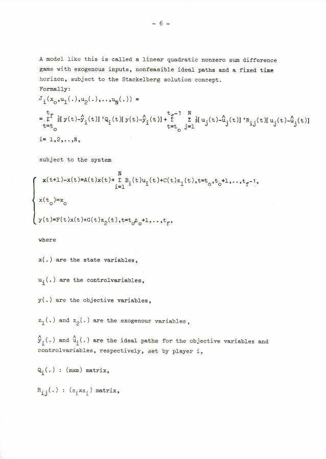
A model like this is called a linear quadratic nonzero sum differencegame with exogenous inputs, nonfeasible ideal paths and a fixed timehorizon, subject to the Stackelberg solution concept.Formally:Ji(xo,ul(.)~u2(.)...,uN(.)) -

- Ef ~IY(t)-Y.(t)l'Q.(t)IY(t)-Y.(t)]tt~-1 E ~Iuj(t)-uj(t)]'Rij(t)Iuj(t)-uj(t)lt-to i i it-to j-1

i- 1,2,..,N,

subject to the system

Nx(ttl)-x(t)-A(t)x(t)t1E1Bi(t)ui(t)tC(t)zl(t),t-to,tofl,..,tf-1,

x(to)-xo

y(t)-F(t)x(t)tG(t)z2(t),t-tdtó 1,..,tf,

where

x(.) are the state variables,

ui(.) are the controlvariables,

y(.) are the objective variables,

zl(.) and z2(.) are the exogenou: variables,

n nyi(.) and ui(.) are the ideal paths for the objective variables andcontrolvariables, respectively, ~et by player i,

Qi(.) : (mxm) matrix,

Rij(.) : (sixsi) matrix,

- 7

A(.) : (nxn) matrix,

Bi(.): (nxsi) matrix,

C(.) : (nxrl) matrix,

F(.) : (mxn) matrix,

G(.) : (,mxr2) matrix.

It is natural to assume the matrices Qi(.) and Ri~(.) tu be positivesemi-definite. To avoid singularities we assume the matrices Rii(.) tobe positive definite.Without loss of generality we assume the matrices Qi(.) and Ri~(.) tobe symmetric.

Player N selects his strategy first, then player N-1, and so on.

4. The Principle of Optimality.

It is important to check , whether the Stackelberg solution conceptsatisfies Bellman's principle of optimality, because, if it is satisfied,we can apply the dynamic programming technique to find a(closed loopno memory) solution for the game.The principle of optimality states, that an optimal strategy for theproblem starting in xo at to must have the property, that the part ofthe strategy, that remains after having applied it some time steps, isalso optimal for the problem starting in the state reached at that pointin time.The Stackelberg solution does not satisfy the principle of optimality.We will show, why this is the case for the model described above, andwe will give a numerical example.The rational behaviour of player 1 can be found by solvirg a standardoptimal control problem, because we can consider the strategies ofthe other players as exogenous inputs. This leads to (see e.g. [2]) :

ul(t)--(R11(t)tBl'(t)Kl(ttl)B~(t))-1B1'(t)(K1(ttl)((ItA)x(t)t

Nt lE2Bi(t)ui(t)tC(t)zl(t))tgl(ttl))tul(t),t-to,totl,...,tf-~

where81(t)-L1(~1(ttl),u2(t),u3(t),..,uN(t)),t-tol,tot2,.., tf-~

It follows, that

81(t) -L2(u2(t),u2(ttl),--,u2(tf-1),u3(t),-.,uN(tf-1)),t-t~tl,tot2,..,tf-1

When we substitute the rational behaviour of player 1 into the systemequations, we find

x(ttl)-L3(x(t),u2(t),u2(ttl).., u2(tf ~),u3(t),..,uN(tf-~)),

t-to,totl,..,tf 1,

Observe, that we don't have a~ystem anymore, because the axiom ofdeterminism or the non-anticipf.tivity is no longer satisfied. It isclear, that in a situation like this the principle of optimalitycan't be satisfied.Example:N-2, T-{to,tl,t2};A(.)-O;C(.)-O;F(-)-1;

B1(to)-1,B1(tl)-o,B2(to)-o,B2(tl)-1;

4,1(t2)-2;Q2(tl)-2;R11(to)-2;R2~(tl)-2

The other cost matrices and the ideal paths are zero.

or: J1-x2(t2)tui(t6)

J2-x2(tl)tu2(tl)

x(to)-xo

X(tl)-X(to)flll(to)

x(t2)-x(tl)tu2(tl)

The rational behaviour of player 1 can be expressed as

ul(to)--~(xotu2(tl))

Sc, i;layer 2 faces the problem:minimize J2x~(tl)tu2(tl)

subject to x(to)-xo

x(tl)-~x(to)-zu2(tl)

x(t2)-x(tl)tu2(tl)

Open loop solution: u2(tl)5 x0'

Linear closed loop no memory solution: u2(tl)a~x~(tl).Both solutions give rise to the same trajectories and the same costs.So, the open loop Stackelberg solution becomes

ui (to)--5o,u2(tl)5xoand the linear closed loop no memory Stackelberg solution becomes

ul(to)--5o~u2(tl)-~x~(tl)

with trajectory

x~`(to)-xo,x~(tl)---25-xo,x~`(t2)--5co .

2Whereas~ starting in 5o at tl (in fact not a game situation anymore),the optimal strategy is u2(tl)-0.

So, the principle of optimality isn't satisfied.A"tree"-example can be found in [7].

The solution, that is found by means of dynamic programming, is called

- 10 -

the feedback Stackelberg solution.The interpretation of this solution is, that in this case each playerwaits with announcing his action until he makes observations aboutthe state of the system, that is realized. In the closed loop no memo-ry solution each player announces at the beginning of the planningperiod, for each point in tim~, how he will react to his observationsabout the state of the system, he selects from all functions of obser-vations and time.In the feedback solution each player announces at each point in time,how he reacts to his observations about the state of the system, thatis realized at that point in time: in fact the principle of optimali-ty is postulated.In the closed loop no memory solution a player can reach lower coststhan in the feedback solution by announcing a strategy, that is on theone hand suboptimal for him for the last part of the game, but on theother hand such that his follower~ while minimizing their own costs,will choose strategies, that lead to trajectories, that are so muchbetter for him for the first part of the game, as compared to the feed-back solution, that the losses in the last part of the game are more thancompensáted. But the closed loop no memory solution is not stable inthe sense that the followers can't be sure, that the leaders willstick to their announced strategies, when the game gets to thestage, where those strategies are inferior to them. Whether theleaders will keep their (suboFtimal) "threats", depends on how theyweigh the actual costs by their credibility in the future.For the feedback Stackelberg solution it isn't true anymore in general,that the leader in the two person game has lower costs than be wouldhave had in the feedback Nash s~lution: a"tree"-example can befound in [ 71 .

In the next paragraphs we will present results on the open loop Stackel-berg solution, where each player announces at the beginning of theplanning period a.strategy, which only depends on the initial stateof the system and time, and results on the feedback Stackelberg solutionfor the model, described in paragraph 3. The closed loop Stackelbergsolution is still a topic of fLrther research; in [9] it is shown,

- 11 -

that the closed loop no memory Stackelberg strategies in this deter-

ministic setting are not linear.

5. Open Loo Stackelberg Solution.

We start with some remarks on the nature of the problem, When we solve

for the rational behaviour of player 1, a standard optimal control pro-

blem, and substitute this rational behaviour in the system equations

a;;d in the cost functionals for the other players, we ~nd up with cost

functionals for the other players, system equations, backward recur-

sive matrix Riccati equations and backward recursive trecking equations,

driven by the strategies of the other players ( a system:), with a fixed

boundary condition at the time horizon.When we eliminate player 1, using the necessary conditicns for his

rational behaviour according to Pontryagin's minimum principle, we

end up with: cost functionals for the other players, system equations

and adjoint system equations, with a boundary condition on state and

adjoint state at the time horizon.Both situations can be viewed upon as the same problem as the original

one with one player less, but constrained by a system ~ith a dimension,

twice as big as the dimension of the original system, a.nd with mixed

boundary conditions. To eliminate player 2 we have to solve this two

point boundary value optimal control problem. Again we can choose

between techniques, based on the "completion of the squere" argument,

and Portryagin's minimum principle (see e.g. [2]).

In the same way the other pla,yers can successively be eliminated.

This leads to a sequence Pi,i-2,3,..,N, of two point roundary value

optimal control problems.The open loop Stackelberg solution follows directly fron, the solution

of PN, the optimal control problem for the leader. The solution of

PN can be found by solving a backward recursive matrix Riccati equation

and a backward recursive tracking equation.

The technique we use in this paper is successive application of Pontry-

agin's minimum principle.

- 12 -

In theorem 1 we state and prove, under the assumption that (ItA)-1exists, how the sequence Pi,i-1,2,..,N, is formed. Implicitly onefinds the rational behaviour ~f the followers in terms of adjoint varia-bles. We will use the symbols p,y and q for the adjoint variables,that show up as a consequence of the elimination process. In theorem2 we state and prove, which Riccati equation and tracking equationhave to be solved to find a solution for PN and how the open loopStackelberg solution relates to the solution of PN.Notation: for notational convenience we won't write the time dependen-cy of the matrices.

Theorem 1-Assuming that (ItA) is nonsing,ilar, the successive elimination of fol-lowers in the N-level Stackelberg linear quadratic difference gamewith an open loop information structure by means of successive appli-cation of Pontryagin's minimum principle leads to the followingsequence of problems:

P1: minimize J1ul(. )

twhere J1- ~

t-t~[ Y(t )-Yl(t )] ' Q1I Y(t )-Yl(t )] t

tf -1 Nt E E ~[u.(t)-u.(t)]'R [u.(t)-u.(t)],

t-t~j-1 J J lj J J

sub.j ect to

x(ttl)-x(t)-Ax(t)t E Bj(uj(t)-uj(t))t L Bju~(t)t cz1(t),J-1 J-1

x(to)-xo

y(t)-F x(t) t G z2(t) , t-to,totl,..,tf.

t-to,totl,...,tf-1,

- 13 -

Pi,-i-2,3,...,N: minimize Ji

u.(.)i

where Jt

i - ~ z[Y(t)-Yi(t)]'Qi[Y(t)-Yi(t)]tt-t 0

t Ef-~ E ~[uj(t)-u~(t)]'Rij[u~(t)-uj(t)]t-to j-1

sab,ject to

a system, consisting of (21-2:~n) dimensional forwardrecursive equations and (21-2xn) dimensional backward recursive eg,ue-tions:

~xi(ttl)-xi(t)-Ai xi(t)tSipi(ttl)tvi(t),t-to,totl,..,tf-1,

xi(to)-[ xo:o. ..o]

n.((2i-2-1)(5.,x .

Y(t)-[ F:o...o] x. (i

and

~

im )

t)tGz2(t),t-to,totl,...,tf.ien )

pi(t)-pi(ttl) - Aipi(ttl)tQixi(t)twi(t)~t-t~1 ,tf-2,..,to~

(5.2)

pi(tf)-Qixi(tf)twi(tf)

where(i) uitl(.),uit2(.)~..,uN(.)

n:((21-2-1)

are exogenous to Pi,i-1,2,..,N.

-1 ~; ~ n(ii) ui(t)-[-R11Bl:o...o] pi(ttl)tul(t),i-2,3,..,N,

n.,((21-2-1)tn)

-1 '' nuj(t)~o ..o:-RjjBj:o...o] pi(ttl)tuj(t),J-2,3,..,i-1,i-3,4,...,N,(2J-2~) : n : ((21-2-2J-2-1)im)

for t-to,tofl,....,tf -~

X2(.)~ X(.),

- - I--i-1( . )

Yi-1(.)

~( 2i-3~tn )

(2~-3~tn),i-3,4,...,N.

(iv ) P2(')~ P1(.),Pi-1(. ) (2i-3im)

Pi-1(.) n

~-1(.) ((21-3-1)~cn)

N N(V) v2(.) o E Bj(uj(.)-uj(.))f r Bjuj(.)tcZl(.),j-2 j -1

N1Bj(uj(.)-uj(.))t E Bjuj(.)tc ~(.)j-1

(vi) w2(.) ~ F'Q1(Gz~(.)-Y~(.)),

wi-I(.)

FrQi-1(Gz2(.)-Yi-1( "wi(.) ~

Pi(.)~ ,i-3,k,...,N.

ó

n

((21-2-1)~!n),i-3,4,...,N.

(2i-3tn)

n

,i-3,4,...,N.

( ( 2i-3-1)~en )

- ~5 -

Á. p diag (A, A, ... , A), i- 2,3,...,N.i -( 2i-2ytn )

.(viii) S2 0-B1R11B1'

where

n ( ( 2i-3-1)~en )

0 0 ((21-3-1)ien)

andUi-1 is a direct sum:

I ~i-1 -Ti-11(2i-3xn)

, i-3,~,..,N,

I-U. ' ~ ( pl-3~ )L i-1 -Si-1

( 2i-3itn ) ( 2i-3xn )

-1 ~Bi-1Ri-l,i-1Bi-1 0 n

Ti-~ ~

~ ~Ui-1~ diag (B1R11Ri-1,1R11B1'B2R22Ri-1,2R22B2'

n n

B3R33Ri-1,3R33B3'~'B4R44Ri-1,~:R44B1~,n n n

0 ,..........,Bl-2Ri12,i-2Ri-l,i-2Ri12,i-2Bi-2, 0).

((22-1)xn) n ( ( 21-~-1)~exs )

- 16 -

(ix) Q2~ F'Q1F,

rQi-1 0 1Qi~

where

( 2i-3ien )

~ 1-.ii-1 -Qi-1 (2 ~)

( 2i-3ien ) ( 2i-3i~n )

0 ~ ((2i-3-1)tn)n ( ( 2i-3-1)ien )

Proof:P1 is immediately clear.P2 up to PN we show by induction.

a) P2 is found by stating the necessary conditions for the solutionof P1, according to Pontry~,gin's minimum principle. These condi-tions express the rational behaviour of player 1. These conditionsare:( x(ttl)-x(t)-ax(t)t E B.(u.(t)-u.(t))t E B.u.(t)tcZ (t)

(5.3) ~

t-tf -1,tf~2,...,to,

~pl(tf)-F'Q1(Fx(tf)tGz2(tf)-yl(tf))

and

(5.5) R11(u~(t)-ul(t))tBi pl(tfl)-o,t-to,totl,..,tf -1.

l.x ( to )-xo'

i-3,~,..,N,

~ Qi-1F 0 n

~-1 J J J ~-1 J J 1 '

t-to,totl,...,tf,-1,

~pl(t)-p1(ttl)-F'Q1(Fx(t)tGz2(t)-yl(t))tA'pl(tfl),

- 17 -

Now we substitute (5.5) into (5.3). It is easily checked, that thieleads to the required form for P2.

b) Pitl is found by stating the necessary condition~ for the solu-tion of Pi, according to Pontryagin's minimum pri~ciple. Theseconditions express the rational behaviour of player i.First we make some preliminary steps.Step 1: we write the constraints of Pi as a system with mixed

boundary conditions by writing the backward recursiveequations as forward recursive equations.

(5.6) pi(ttl)-(ItAi)-1(pi(t)-~iXi(t)-wi(t))~t-to,totl,..~tf-1.

This leads to the system

X. X. A. O S. . ~. ~ -Q. . I~ X.(5.7) H1 (ttl.)- 1( t)-( 1 t 1(ItÁi~)-1 i. ) Ni (t)-pi pi o-I I p,

i

i vi(t)- (ItAi~)-lwl(t)t ~t-to,totl,... tf1~ ,0

with initial boundary condition :( I:o] x1

r 1

~ (to)-X00ó

and final boundary condition :

~ -Qi. I~ Xl (tf)--wi(tf).

P

Step 2: we rewrite the cost functional Ji, using (ii), (iii),

Pi

i

S

I

(viii) and (ix).

- ~8 -

.l tf(5.8) Ji- s ~{zi(t)vixi(t)t2.z1(t)

t-t0F~Qi(Gz2(t)Yi(t))

0ó

t(Gz2(t)-Yi(t))~Qi(Gz`(t)-Yi(t))} t

tf 1

f Et-t0

t

2{pi(ttl)Uipi(ttl)f(ui(t)-ui(t))'Rii(ui(t)-ui(t)) f

N n ~t E (u~(t)-u~(t)) Rl~(u~(t)-u~(t))}.,j-it1

Step 1 and step 2 only consisted of rewriting problem P..iWe proceed with stating the Hamiltonian functional for P. andiwith stating the necessary conditions for the solution of P..iStep 3: we define the Hamiltonien functional Hi, using (5.6).

~ ti~(5-9) Hi(t~xi~Pi~ui~pi~qi~Yi)-~xiVixi t x.i 'Qi(Gz2(t)-Yi(t)) f0

ó

f~[pi-Q.ixi-wi(t)l ~ (ItAi)-lUi(ItAí)-1 Ipi-Q,ixi-wi(t)] t

t~[ui-ui(t)l~-Rii[ui-ui(t)l t

~' ~. ,~pi:qi:yi) {(

( IfA ~ ) -1~ -Q1 ÏI)

i )

N Ns. Ei(ui-ui(t)) E B.(u.(t)-u.(t))t E B.u.(t)tcZ (t)1(I~á ')-lwl(t) t o t j-if1 ~ J ~ o.7-1 ~ J 1 }I ó '

ó

- 19 -

Step ~: according to Pontryagin's minimum principle there existr~ ~~ ~

[Pi:qí:yi](t)~t-to,totl,..tf,ao and al~

such that the following equations are satisfied ( see e.q. [10]):

1) the contraints of problem Pi.

2) ax.aul (`',Xi(t),Pi(t),ui(t),pi(ttl),qi(ttl),yi(ttl))-o ~

~Rii(ui(t)-ui(t))tBipi(ttl)-o ~

~~i(t)--Riibipi(ttl)tui(t)~t-to,totl,..,tf - 1 (5.10)

3) the backward recursive adjoint equations

piqil (t)-

Lyi~

[oi

~ ,.o -Qi ~ [ Si :I]

-( t (Itql)-I I

~-Qi

t

I

I

piqi

yi

o -

pi) qi

yi

(ttl)t

(ItAi)-1 Ui(ItAi~ )-1 [~i(t)-QiXi(t)-wi(t)] t

t (V.X.(t) t1 1

pi

F~Qi(Gz2(t)-Yi(t))O

t-tfl,tf2,..,to, (5.11)

Ai

aHi

(ttl)- - (t,zi(t),Pi(t),ui(t),p i(ttl),qi(ttl)~yi(ttl)) x

a I Xi~

4) the transversality conditions

- 20 -

Pi

qi

Yi

(to )-

(tf)-

[:~ ao

nl t

(ttl)-qi

Step 5: we rewrite the necessary conditions; using (5.6) we cansplit (5.11) into

(5.15)

Yi(t)-(ItAi)-1 (S1~

t-to,totl,..~tf -1.

and

Pi

qi

(Vixi(tf)t

(ttl)fyi(ttl)tUipi(ttl)~

P. P- ~ P-1 (t)- 1 (ttl)-Ai i

ql ql ql

F'Qi(Gz2(t)-Yi(t)0

t :

fr~m (5.14) we find

(5.12~

F,Qi(Gz2(tf)-Yi(tf))0

ó

Yi(t)tViXi(t)f

, t-tf-l,tf-2,..,to;

(5.16) Yi(ttl)-Yi(t)-Aiyi(t)-UiPi(ttl)-Si~lpil (tt1),qi

d

)(5.13)

t-to,totl,..~tf-1:

- 21 -

from (5.12) and ( 5.13) we find

(5.17) Yi(to)-o

and

F'Q.(Gz (t ) y.(t ))(5.18) pll (tf) --QiYi(tf)tVixi(tf)t

i 2o f i f

ql~ o .

Now we substitute (5.10) into vi(t) and regroup the fo~-ward recursiveequations (5.1),(5.16) and (5.17) as well as the backirard recursiveequations (5.2),(5.15) and (5.18). It is easily checkF3, that thisleads to the required form for Pit1,Q.E.D.

Theorem 2:The N-level Stackelherg solution for the linear qixadratic differeneegame with an open loop information structure is given by

ul(t)~ -R11Bl:o...ol(x(ttl)~tl(ttl)t6(ttl))tul(t)(5.19) n.((2N-~-1)icn)

u~(t)~ o...o:-R~~B~:o...o](K(ttl)xN}1(ttl)tg(ttl))tu~(t),(2~-2xn): n :((2N-~-2~-2-1)i:n)

,7-2,3,..,N,t-to,totl,..,tf -1

where

xN}1(t),t-to,totl,..,tf,is the solution of the system

- 22 -

(5.20 )

xN}1(ttl)-(I-SNt1K(ttl))-1((It~tl)~fItl(t)}SNt1B(ttl)fvNtl(t))~

t-to,totl,..,tf 1,

(5.21

and

K(t),t-totl,totp,,,,tf, is the solution of the backward recursivematrix Riccati equations

K(t)-QNtlt(ItÁNtl)K(ttl)(I-cNtlI{(ttl))-1(ItÁN}1),

K(tf) - QNt1

and

g(t),t-totl,tot2,..,tf, is the solution of the backward recursivetracking equations

rg(t)-wNt1(t)t(ItáNtl)g(ttl)t

(5.22) t(It 1vt1)K(ttl)(I-SNt1K(ttl))-1(SN~lg(ttl)tvNtl(t))~

t-tf 1,tf2,...,totl,~B(tf)-wNt1(tf)

and

xNtl(')'v Ntl(')'wNtl(')'~tl'SNtland QNtl are defined in the sameway as xi(.),vi(,),wi(.),Ái,Si and Qi for i-3,~,..N in theorem l.

Proof:From theorem 1 we know, that we can find the N-level Stackelbergsolution for the linear quadratic difference game with an openloop information structure by solving PN, the optimal control pro-blem for the leader. We can áo this by following the same reasoningas for Pi in part (b) of the proof of theorem 1. This leads to theopen loop Stackelberg solution

t-tf 1 ,tf2.,...,totl

- 23 -

u~(t) - I-R11 B1;o...o]PNt1(tt1)tu~(t),

(5.23) n:((2N-~-1)~tn)

u~(t)-lo...o.-RJJB~:o...o)PNtl(ttl)fu~(t)~J-2,3~..~h~

(2J-2tn);n :((2N-1-2J-2-1)xn) t-to,totl,...,tf 1

where

~~tl(.) is defined in the same way as pi(.) for i-3,4,..,N in': h~-orem 1

and

pNtl(t),t-to}l,tot2,..,tf, is part of the solution of the two pointboundary value problem

XIVtl(ttl)-XNtl(t)---Nt1XNt1(t)}SNt1pIVt1(ttl)tvNtl(t),t-tóotl,..,tf-~ e~' ~

XNtl(to)-~XO:o...o](5.24)

pNtl(t)-pNtl(ttl)- 7Vt1pNt1(ttl)tQNt1XNt1(t)~Ntl(t)~t-tf-l~tf-2~..~to~

This two point boundary value problem can be solved in the usuel wayby postulating the linear relationship~rrtl(t)-x(t)~tl(t)tg(t),t-to,totl,...,tf-

~Ii tl(tf)-,TltlXntl(tf)~Ntl(tf)'

The recursive equations ('S.20),(5.21) and (5.22) folluw immediately.Q.E.D.

Remarks:1) The costs can immediately be calculated from the cos`c functionals,

taking into account that

Y(t)-~F;o..o]xN}1(t)tGz2(t)~t-to,totl,...,tf.n :((2N-1-1)~n)

-24-

2) It is not clear directly under which conditions in terms of thedata of the game the matrices (I-SNt1K(.)) are nonsingular, althoughwe can prove in an indirect way, that the open loop Stackelbergsolution exists(and is unique) under the conditions, that Qi(.) andRi~(.) are positive semi-definite and Rii(.) are positive definite.In section 6 of this paper we show, that the feedback Stackelbergsolution exists (and is unique)under those conditions.Furthermore we use the fact, tY,at for a one stage problem the openloop solution and the feed~ack solution are identical. We can trans-form our problem into a one stage problem by defining (see e.g. ~8j)x(1)a(xr(totl)x~(tot2)....x~(tf)]~

x(o)~[x~ x.~....x~j ~- - o 0 0

ui(o)~[ui(to)ui(totl)...ui(tf 1)]~,i-1,2,..,N,etc....

The cost matrices for this one stage problem are

Qi(o)~ diag ( Qi(to),o,...,o)

e,i(1)a aiag ( Qi(totl),Qi(tot2),...,Qi(tf))Ri~(o)~ diag (Ri.7(to),Ri~(totl),...,Ri~(tf1))Finally we note, that Qi(.) s.nd Ri~(o) ~e positive semi-definite,if Qi(,) and Ri~(.) are positive semi-definite,and that Rii(o) ispositive definite, if R..(.) are positive definite.iiThe method described here is not attractive, if the planning periodis long, because in that case the dimensions of the problem becomevery big.

Fxample :

We will elucidate theorem 1 and theorem 2 by means of a simple twostage two person nonzero sum linear quadratic difference game.The open loop Stackelberg solution for this game was also calculated

-25-

in a straightforward way in [ 8] .

Cost functionals:J1-2x2(1)t2X2(2)tui(o)tui(1)

J2-x2(1)fx2(2)fu2(o)}u2(1)

System: (x(ifl)-x(i)tul(i)fu2(i),i~0,1,

{(x(o)-xo

A-o,B1-1,B2-1,C-o,F-1,G-o,

n n n nRi~-o,i~.7,Y1-yZu1-u2-o,

Ql(2)-4,4,1(1)-4,Q1(o)-0,

Q2(2)-2,Q2(1)-2,Q2(o)-0,

R11(1)-2,R11(o)~2,R22(1)-2,R22(o)-2.

First ve construct A3,S3(.),Q3(.)'v3 and w3.

Á30 0 ~

S3(1)--~ -~

;S3(o)- - ~ -~ ~ v30~0 0 ~o ~] [o ~,

4 0 4 0 0 0Q3(2)- 2-~ ; Q3(1)- 2-~ ; Q3(o)-

Lo o] ~w30.

From (5.21) ve find

4 0 26~5 k~5K(2)- ; K(1)-

2 -4 11~5 -26~

Fron (5.22} ve find g(2)-o;g(1)-o.

From (5.20) ve find

36~145 x 13~145 xx(o}- xo ; a(1}- o; z(2)- o3 0 3 u~1~5 xo 3 8j1~5 x~

From (5.19) we find the open loop Stackelberg solution

ul(o)- -~ xo;ul(1)--165 xo;

u2(o)--1~5 xo ;u2(1)- 145 xo.

6. Feedback Stackelberg Solution.

The feedback Stackelberg solution is by definition the sólutionfor the game, that is found by means of dynamic programming.As always, when we apply dynamic programming in linear quadratic

frameworks, we have quadratic value functions for all players and

we will operate on the backward recursive equations for those value

functions.

Notation: for notational convenience we won't write the time depen-

dency of the data-matrices.

The value function Vi(.,x) for player i,i-1,2,..,N, satisfies the

backward recursive equations

Vi(t,x)- min {z[FxtGz2(t)-ni(t)I~Ql[FxtGz2(t)-Yi(t)Itui(t)

Nt E z[uj(t)-uj(t)] ~~ij[uj(t)-uj(t)]t

j-1

tV.(ttl,(ItA)xt E tsj[uj(t)-uj(t)]tE Bjuj(t)tCz~t))},1 j-1 j-1

t-tf 1,tf2,..,to. (6.1)

Vi(tf,x)-~[FxtGz2(tf)-yi(tf)]Q1[FxtGz2(tf)-yi(tf)] (6.2)

The optimal behaviour of player i,i-1,2,...,N, at time t can be foundby differentiating the right hand side of (6.1) with respect toui(t) and setting this derivative equal to zero. In remark 2 atpage 37 we show, that the Hessian matrix is positive definite (because

we assumed the matrices Qi and Rij to be positive semi-definite andthe matrices R.. to be positive definite), so that the

iiu,(.),i-1,2,..,N, calculated according to the described procedure,i

will indeed minimize the cost functionals. Remember, that theStackelberg solution concept presupposes, that the decision of

player i,i-1,2,..,N-1, depends on the decisions of the players higher

in the hierarchy, that is the players itl up to N.To solve for the optimal behaviour of player i,i-1,2..,N, we define

the quadratic value functions as follows:~ ~

~~~y(tex)-zx Ki(t)Xtgi(t)xtci(t)~t-t~,tptl,..,tf„1-1,2,..,N.

Without loss of generality we assume the K- matrices to be symmetric.

The descríbed procedure, that is the equalizing of the gradients with

respect to u.(t) of the right hand sides of (6.1) with zero, leadsi

to the following set of equations.

NRll[ul(t)-ul(t)]tBl(Kl(ttl)((ItA)xt E Bj[uj(t)-uj(t)]t

j-1N

t E B.í~.(t)tCz (t))tg (ttl))-o (6.3)J Jj-1

andi-1 au.(t) , i-1 au.(t) ,

Rii[ui(t)-ui(t)lt E(au,(t) ) Rij[uj(t)-uj(t)]~(Bit É au(t) ~j).j-1 i j-1 i

N ~ N ~,(Ki(tt~((ItA)xt E Bj[uj(t)-uj(t)]t E Bjuj(t)tCzl(t))tgi(ttl))-o,

j-1 j-1

i-2,3,..N (6.~),

t-to,totl..,tf-1.

Notation: the sum-term E and the product-term II should be under-stood as follows:if the index is nondecreasing, as normal, and if the index is

decreasing, E- o and n- I.

Theorem 3:

The set of equations (ó.3) and (6.~) have the following solution:

-28-

ui(t)--Di(t)((ItA)x} E Bj[uj(t)-uj(t)]f E Bjuj(t)tcZl(t))tj-it1 j-1

Nt E (-D1R)(t))SR(ttl)tui(t),i-1,2,..,N,t-to,totl,..,tf 1 (6.5)~-1

where

Dil)(t ~(R11tB1Kl(ttl)B1)-1B1;DiR)(t ~o,R-2,3,..,N (6.6)

D1(t)-Di1)(t)Kl(tti)

t-to,tatl,..,tf1and

(6.7)

~ i-1 i-1 , ,Di(t)-Mil(t)Bi{ E ( II (I-BkDk(t))) Dj(t)Rij~

j-1 k-jt1i-1

.D.(t)( n (I-B D (t)))f~ k-jt1 k k

i-1 , i-1t( N(I-B D.(t))) K.(ttl)( II(I-B D(t)))} (6.8)k-1 k k i k-1 k k

DiR)(t)-Mil(t)Bi{ lEl(lIIl (I-BkDk(t))i1-Dj(t)Rij.j-1 k-j}1

(2) i-1 m-1 (~,).(D. (t)-D.(t) L ( II (I-B D (t)))B D (t))t

~ ~ m-jtl k~jtl k k m m

i-1t( II (I-BkDk(t)))~Ki(tfl).

k-1

i-1 m-1 ( ~, ).( E ( II (I-BkDk(t)))(-BmDm (t)))},

m-1 k-1

Q-1,2,...,i-1

(i) 1 , i-1 ,Di (t)-Mi (t)Bi( n (I-BkDk(t)))

k-1

(6.9)

(6.10)

-29-

(~.)Di (t)-o,k-itl,it2,..,N

where

, i-1 i-1 , ,Mi(t)-RiitBi { E ( R (I-BkDk(t))) Dj(t)Rij.

j-1 k-jt1i-1

.D.(t)( n (I-B D (t)))tJ k-jt1 k k

(6.11)

i-1 , i-1t( II(I-BkDk(t))) Ki(ttl)( n(I-BKDk(t)))} Bi (6.12)

k-1 k-1

for i-2,3,..,N, t-to,totl,...,tf -1

Before we prove theorem 3 we will first state and prcVe some usefullemmas.

Lemma 1~

n n na) I- E Pi( n (I-Pk))- R(I-Pk)

i-~ k-itl k-j

n n k-1 n k-1b) ï{Pi-Pi E ( II (I-PR))Pk}- E( n(I-PQ))Pk

i-,7 k-it1 k-it1 k-j R-j

Proof:n n

a) I- E Pi( II (I-Pk))-(I-P )-P 1(I-P )-i-~ k-it1 n n- n

n-Pn-2(I-Pn-1)(I-Pn)-...-Pj( lI (I-Pk)~

k-jtl

n- n (I-Pk),Q.E.D.

k-j

- 30 -

b)n n n k-1E P.- E P. E ( II (I-P ))P -

i-j 1 i-j 1 k-it1 k-it1 Q k

n n k-1 k-1- E Pi- E E Pi ( n ( I-PQ ))Pk -

i-J k-jtl i-J R-it1

n k-1 k-1- P.t E (I- E P.( II (I-P )))P

J k-jt1 i-j 1 R-it1 ~ k-

n k-1~ ~ ~f k-jt1 ~-j

le~,a .1.a. ,n k-1

- E ( JI (I-PQ ))P , Q.E.D.k-j Q -j

Lemma 2~

k

For j-2,3,..,N,t-to,totl,..,tf-1 we have:suppose, that (6.5) is corrFct for i-1,2,..,j-1, thenau.(t) , j-1 , ~-~ B ( n (I-B D (t))) D,(t),i-1,2,..,j-1 (6.13)auj(t) - j k-it1 k k 1

Proof:We prove this by backward induction:

1) i-j-1:au.i-1(t) , ~auj(t) ? BJDj-1(t).

(6.5)2) Suppose, that (6.13)is correct for i-j-l,j-2,..,kt1

auR t) J-1 aui(t) , , ,i-u,:au~ -(lERtl(auJ(t))LitB~) r,R(t)-

(6.5)

- 31 -

j-1 r j-~- r r r r r- -( E (-B.( n (z-B D ( t))) D.(t))B.tB.)D (t)-fi i-Rf1 Jk-it1 k k i i J Rinductionassumption

r J-1 J-1 r r r r- -B.(I- E ( II (I-B D (t))) D. (t)B.jD (t)~

J i-R,t1 k-it1 k k i i E

r J-1 r r- -B.( n (I-B D (t))) D (t).T J k-Rt1 k k klemma la

Q.E.D.

Lemma 3:For j-2,3,..,Ntl,t-to,to}1,..,t~-1 we have:

suppose, that (6.5) is correct for i~1,2,..,j-l,then

j-1ui(t)-ui(t)--Di(t)( II (I-BkDk(t))).

k-it1

N N.((ItA)xf E Bm[umt)~zm(t)]f E ~mum(t)iCzl(t))f

m-J m-1

N ( Q 1 j-1 m-1 (~ )t E(-Di lt)tDi(t) E ( n (I-BkDk(t)))BmDm (t)).

R-1 m-it1 k-it1

. gR(ttl),i-1,2,..~J-1.

Proof:We prove this by backward induction.

1) i-j-1: (6.5) immediately implies (6.14).2) Suppose, that ( 6.1~) is correct for i-j-l,j-2,..,nt1;

(6.14)

i-n:

- 32 -

un(t)-un(t)--Dn(t)(~tA)xt E Bm[um(t)-um(t)]t E Bmum(t)f4 m-nt1 m-1

(6.5)

Ntczl(t)) f E (-Dn~ )(t) )BR(ttl)-

~-1

j-1 j-1.~-Dn(t)((ItA)xt E Bm{-Dm(t)( II (I-BkDk(t))).induction m-nf1 k-mt1assumption

.((IfA)xt REJBR[uR(t)-uR(t)] t RE1BRuR(t)}cZl(t))t

N ~ j-1 i-1 ~t E (-DmR~(t }tDm(t) E ( n (I-BkDk(t)))BiDiR'(t))SR(ttt)}t

1t-1 i-mtl k-mt1

N N Nt E Bm[um(t)-um(t)]} E Bmum(t)fczl(t))t REi(-DnR)(t))BR(tt1)-

m-j m-1

j-1 j-1--D (t){I- E B D (t)( B ( I-BkDk(t)))},

n m-nfl m m k-mf1

.((Ifa)xt E ~Q[ uR(t)-uR(t))t E BRu~t)tcZl(t))t1C- j R-1

N (R,) j-1 (R)t i {-D (t)tJ (t)( E (B D (t)-

R-1 n n m-nt1 m m

j-1 i-1 (R)-BmDm(t) E ( II (I-BkDk(t)))BiDi (t)))} gR(ttl).

i-mt1 k-mt1

From this, lemma la and lemma lb, (6.1k) for i-n is immediatelyclear.Q.E.D.

-33-

Now we are ready tc prove theorem 3.Proof theorem 3:We prove this by induction.

1) We rewrite ( 6.3) as follows:ul(t)--(R11tB1K1(ttl)Bl)-1B1(Kl(ttl)((ItA)xt

N Nt E Bj[uj(t)-uj(t)It E Bjuj(t)tcZl(t))tal(ttl))tul(t),

j-2 j-1

t-to,totl,..tf 1.

From this, (6.5) for i-1, (6.6) and (6.7) are immediately clear.

2) Suppose, that the solution of (6.3) and (6.~) for i-1,2,..,j-1 isgiven by (6.5) up to (6.12) for i-1,2,..,j-1, then, using lemm~, 2and lemma 3, we can rewrite (6.4) for i-j as Pollows:

Rjjluj(t)-uj(t)}tJEl{-Bj(JII1 (T-BkDk(t)))~-Di(t)}R`l.i-1 k-it1

.{-Di(t)(JII1 (I-BkDk(t)))((ItA)xt E Bm[um(t)-um(t)}tk-it1 m-,7

NtmElBmum(t)tCzl(t))t

N (R) j-1 m-1 (JC)t E(-D. (t)tD.(t) E ( n (I-B D(t)))B D(t))g (ttl)}tR-1 1 1 m-it1 k-it1 k k m m R

1t(B~tJE {-B~(Jnl ( I-g D (t)))~D~(t)}B~).

~ i-1 ~ k-it1 k k 1 1

j-1 j-1.(K.(ttl)((ItA)xt E B.{-D.(t)( n ( I-B D (t))).

~ i-1 1 1 k-it1 k k

-3~-

.((ItA)xtmEJBmlum(t)-um(t)jt mElBmum(t)tCzl(t))t

N (R) j-1 m-1 (R)t E(-D. (t)tD.(t) E ( II (I-B D(t)))B D (t))g (tfl)}t1L-1 1 1 m-if1 k-it1 k k m m R

t E Bi[ui(t)-ui(t)]t E Biu~(t)tCzl(t))t8j(ttl))-o,i-j i-1

t-to~totl,..,tf-1.

From lemma la we know, that

B~(I-JEl(Jnl ( I-R~ D (t))1~D~(t)B~)-~ i-1 k-it1 -k k 1 1

1-B~(JII (I-BkDk(t)))~,t-to,totl,..,tf -1.

k-1

From lemma lb we know, that

j-1 (R) j-1 m-1E {-BiDi (t)fBiDi(t) E ( II (I-BkDk(t)))BmDmR)(t)}~

i-1 m-it1 k-it1

j-1 m-1 (R)- E ( II (I-BkDk(t)))(-BmDm (t)~t-to,totl,..,tf 1.m-1 k-1

Now it is easy to derive (6.5) and (6.8) up to (6.12) for i-j.Q.E.D.

In fact we have found in theorem 3 the feedback Stackelberg solu-tion in terms of Ki(.) and gi(.),i-1,2,..,N.In theorem 4 we will state and prove backward recursive equationsfor Ki(,) and gi(.),i-1,2,..,N.

-35-

Theorem 4:The feedback Stackelberg solution is given by (6.5) up to (6.12),if Ki(.),i-1,2,..,N, satisfies the backward recursive matrixRiccati equations

N NKi(t)-F~QiFt(IfA) ~{ E ( II ( I-BkDk(t))) ~D~(t)Rij.

j -1 k-j tl

N N.Dj(t)( II (I-BkDk(t)))t( II (I-BkDk(t)?)~Ki(ttl).

k-jtl k-1

N.( II (I-BkDk(t)))}(ItA)~t-tf1 ,tf2 D...~tofl (6.15)k-1

Ki(tf)-F'QiF (6.16)

ar.d gi(.),i-1,2,..,N,satisfies the backward recursive trackingequations

Bi ( t )-F ~Qi ( Gz2 ( t ) -Yi ( t) }f( ItA ` ) .

N N ~ ~ N.{ E ( I[ (I-BkDk(t))) Dj (t)Rij(Dj(t)( R (I-BkDk(t))).j-1 k-jt1 k-jtï

N.(JE1Bjuj(t}tcZl(t))t

t E(D~~)(t)-D.(t) E(mIIl (I-B D(t)))B D(~}(t)) (ttl))tQ-1 ~ ~ m-jt1 k-jf1 k k m m ~

Nt( II (I-BkDk(t)))1(Ki(ttl)(( II (I-BkDk(t)})(JE1Bjuj(t)tczl(t))t

k-1 k-1

-36-

N N :m-1 (k)t E E ( II ( I-BkDk(t)~)(,BmDm (t))BR(ttl))f8i(ttl))~R-1 m-1 k-1

t-t~l~tf-2~..,tot1

8i(tf)-F~,~i(Gz2(tf)-Yi(tf)).

(6.17)

(6.~8)

Proof:Remember, that we had the quadratic value functions

Vi(t;x)-~x~Ki(t)xtgi(t)xfci(t),t-to,totl,..,tf,i-1,2,..,N.Now (6.2) immediately implies (6.16) and (6.18).

From (6.1), theorem 3 and iemma 3 for j-Nt1 we know

~x~xi(t)x~iit)xtci(t)-~JE1[ uj(t)-uj(t)] ~Rij[ uj(t)-uj(t)] t

t~[FxtGz2(t)-yi(t)] ~Qi[FxtGz2(t)-yi(t)]t

N Nt~I(ItA)xfJE1Bj[uj(t) uj(t)]t E Bji~j(t)tCzl(t)]~.

j-1

N N.Ki(ttl)[(ItA)xtJE A~[uj(t)-zj(t)]t E1Bjuj(t)tczl(t)]t

1 j-

fgi(ttl)f (ltn)xtJElB~[uj(t)-uj(t)1tJElBjuj(t)tczl(t)]t

tci(ttl)~t-tf -1,tf -~,..,t t1,0

where

N Nu.(t)-u.(t)--D.(t)( n (z-B n (t))X(ItA)xt E B.u.(t)tcz (t))tJ J J k-jt1 k k J-1 J J 1

-37-

N (JC) N m-1 (k)t E(-D. (t)}D.(t) E ( II (~ BkDk(t)))BmDm (t))BR(ttl).Q-1 J J m-Jt1 k-jt1

Comparing quadratic terms in x and linear terms in x leads to(6.15) and (6.17), respectively, using lemma la and lPmma lb in the

same way as in the proof of theorem 3.Q.E.D.

Rer.iarks :

1) If one is interested in the costs of the game, one sh~uld also eva-luate the constant terms ci(.),i-1,2,..,N.

2) By inductive reasoning we can show, that the Hessian matrices(R11tB1Kl(.)B1) in (6.6) and Mi(.),i-2,3,..,N, in (6.12) are positivedefinite, hence nonsingular, so that minimum costs, Di(.) andKi(.),i-1,2,..,N, exist.First we note from (6.16), that Ki(tf) are positive semi-definite,

because Qi are positive semi-definite.Next we will describe the induction steps in t and i.Suppose Ki(ttl) are positive semi-definite. Because Rij are positivesemi-definite and R.. are positive definite, we can conclude, that, ii

a) (R11tBiK1(ttl)B1) is positive definite, so that from (6.6) and(6.7) D1(t) exists,

b) if Di(t), i-1,2,..,j-l, exist, then from (6.12) Mj(t) is positivedefinite, so that from (6.8) Dj(t) exists.From (6.15) we note, that, if Di(t), i-1,2,..N, exist, then Ki(t)are positive semi-definite, because Qi, Rij and Ki(ttl) are positivesemi-definite. Q.E.D.

3) The system, driven by the feedback Stackelberg soluticn, can bewritten as follows, using lemma 3 for j-Nt1 and lemma la:

N Nx(ttl k(II (I-BkDk(t)))((ItA)x(t)t E Bjuj(t)tCzl(t)),t-to,totl,..tf 1

k-1 j-1

x(to)-xo

-38-

4) The algorithm for the feedback Stackelberg solution has a loop back-ward in time, consisting of the equations (6.15) up to (6.18) and(6.6) up to (6.12), and a loop forward in time, consisting of (6.5)and the system equations.

Example:We will elucidate theorem 3 and theorem 4 by means oP the same exampleas was used on page 24.First we note from (6.17) and (6.18), that gl(2)-g2(2)-g1(1)ag2(1)~0.So, it is of no use to calculate D~R)(t),i-1,2,R~1,2,t-0,1.iFrom ( 6.16) we find

K1(2)-4;K2(2)-2.From ( 6.6)and ( 6.7) we find D1(1) 3.

From (6.12) we find M2(1)9.

From ( 6.8) we find D2(1) 10

From (6.15) we find

K1(1) 2~;K2(1)r.

127From ( 6.6) and ( 6.7) we find D1(o) -i77.

From ( 6.12) we find M(o) 6~2 31329'

From ( 6.8) we find D2(o)-3~9.

From (6.5) and the system equations we find the feedback Stackelberasolution

u2(o)- - 3~9xo;u1(o)- - 34079 0~

-39-

u2(1)- - 8~79xo;u1(1)- - 34o79xo'

with trajectory xo, 8~o79xo' 3~xo~

8. Conclusion.

In this paper solutions are derived for the N-level Sts.ckelberglin~ar quadratic difference game with exogenous inputs~ nonfeasibleiutal paths and a fixed time horizon for two information structures.A topic of further research could be the closed loop informationstructures for this game. In a second paper on this subject we willconsider more players on the same decision level an~ we will givean application in the form of a small linked econometric model forthe Common Market.

Acknowledgement.

I would like to thank Joseph Plasmans from Tilburg and Frank Claeysfrom Gent for reading the manuscript.

References.

1. Plasmans, J.E.J., "Linked Econometric Models as a Difference Game;Nash Optimality", Research Memorandum, Tilburg University, 1978.

2. Plasmans, Joseph E.J. and de Zeeuw, Aart J., "Pareto Cptimality andIncentives to Cooperate in Linear Quadratic Difference Games", ResearchMemorandum FEw 75, Tilburg University, September 1978.

3. Medanic, J, and Radojevic, D., "Multilevel Stackelberg Strategies inLinear-Quadratic Systems", JOTA, vol. 24, pp. 485-~97, 1978.

4. Gardner, jr., B.F. and Cruz, jr.,J.B., "Feedback Stackelberg Strategyfor M-level Hierarchical Games", IEEE, vol. AC-23, no. 3, pp. k89-~91,June 1978.

5. Cruz, jr., Jose B., "Leader-Follower Strategies for ldultilevelSystems", IEEE, vol. AC-23, no.2, pp. 244-254, April 1978.

6. Simaan M. and Cruz, jr., J.B., "On the Stackelberg Stïategy in Nonzero-

Sum Games", JOTA, vol. 11, no. 5, pp. 533-555, 1973.7. Simaan M. and Cruz, jr., J.B., "Additional Aspects of the Stackel-berg Strategy in Nonzero-Sum Games", JOTA, vol.ll, no,6, pp. 613-626,1973.8. Olsder, Geert Jan, "Information Structures in Differential Games",in "Differential Games,and~Control Theory II", edited by Emilio 0.Roxin, Pan-Tai Liu and Robert L.~~~~b~~gf Ma,z.cel Dekker, Inc.,New York and Basel, pp. 9g-135, 1977.9. Medanic, J., "Closed-Loop Stackelberg Strategies in Linear-QuadraticProblems", IEEE, vol. AC-ê3, no.4, pp. 632-637, August 1978.10. Varaiya, p,p, "Notes on Optimization", Van Nostrand Reinhold Company,New York, 1972.

~ u iiiMi~ï~~iii iiii wMïiïa~u ~