SUBMIT TO IEEE TIP 1

Motion-Aware Gradient DomainVideo Composition

Tao Chen, Jun-Yan Zhu, Ariel Shamir, and Shi-Min Hu∗

Abstract—For images, gradient domain composition methods like Poisson blending offer practical solutions for uncertain objectboundaries and differences in illumination conditions. However, adapting Poisson image blending to video faces new challengesdue to the added temporal dimension. In video, the human eye is sensitive to small changes in blending boundaries acrossframes, and slight differences in motions of the source patch and target video. We present a novel video blending approachthat tackles these problems by merging the gradient of source and target videos and optimizing a consistent blending boundarybased on a user provided blending trimap for the source video. Our approach extends mean-value coordinates interpolation tosupport hybrid blending with a dynamic boundary while maintaining interactive performance. We also provide a user interfaceand source object positioning method that can efficiently deal with complex video sequences beyond the capabilities of alphablending.

Index Terms—gradient domain, video editing, mean-value coordinates, Poisson equation, seamless cloning.

F

1 INTRODUCTION

Video composition is very useful in the film, televisionand entertainment industries. Such composition takes aframe sequence from a source video, usually extracting aforeground object (here called a ‘patch’), and pastes it ontoa frame sequence in a target video. This process involvestwo challenges: extracting the patch from the video, andcomposing it with the target frames. In both cases a usermust typically be involved in the process, both to choose adesirable source patch, and a composition location in spaceand time. The main focus of video composition techniquesis to lower the amount of manual effort needed in thisprocess.

Many works related to image and video matting andcomposition have been proposed in computer graphics andimage/video processing (see [1], [2], [3], [4]). Recent workcan even deal with transparent and refractive objects [5].These techniques use alpha-blending composition and focusmainly on how to cut out the alpha-matte of the video-patch from the source video. Compositing using alpha-blending provides good results for scenarios where thesource and target videos specifically have similar illumi-nation conditions, the object is easily separable from itsbackground, and the videos do not differ too much interms of motion, including both global camera motion andlocal object/texture motion. Uncertain object boundaries,due to significant motion blur, smoke or dust, or varying

This work was supported by the National Basic Research Project of China(Project Number 2011CB302205), the Natural Science Foundation of Chi-na (Project Number 6113300861103079), National Significant Science andTechnology Program (Project Number 2012ZX01039001- 003), NationalHigh Technology Research and Development Program of China (ProjectNumber 2013AA013903) and the Israel Science Foundation (grant no.324/11).T. Chen, J.-Y. Zhu and S.-M. Hu are with TNList, Department of ComputerScience, Tsinghua University, Beijing 100084, China.A. Shamir is with The Interdisciplinary Center, Israel.∗ The corresponding author.

illuminations conditions, make it difficult to achieve highquality composition using alpha matting.

For images, gradient domain blending solves such problemsby transferring the gradient of the source image patch tothe target image while maintaining a seamless blendingboundary and correcting illumination differences. This canbe done by solving a Poisson equation, or by interpolationusing mean-value coordinates (MVC), the latter providinginteractive rates of composition [6].

The main challenges in gradient domain video blending,as opposed to image blending, come from motion. Firstly,even if blending results for each individual frame looksatisfactory, the blending boundaries in adjacent framesmay not be consistent, and ‘popping’ artifacts may appear.Secondly, the motions of the source and target gradientfields are typically different and can cause motion artifactseven if the blending boundaries are consistent over time.Thirdly, camera motion differences often exist between thesource and target videos, and there is a need to align them.

Our motion-aware gradient domain video blending tech-nique addresses the above issues. The key idea is to use soft,rather than hard, boundaries between the foreground andbackground for composition inside the blending region. Ineach frame, the real boundary of the source patch lies insidethe blending region, but its exact location can be adjusteddynamically through time. This allows greater flexibility todetermine dynamic boundaries for complex moving objects,and allows fast updates for user interaction, e.g. if the userchanges the position of the source object. Moreover, weuse a novel method for combining the gradient fields ofthe source and target videos inside the blending region.We reconstruct a mixing-gradient field based on consistencyand gradient saliency of the source and target videos. Themixing gradient disperses motion differences across theblending boundary between the source and target videos in-

SUBMIT TO IEEE TIP 2

(a) (b) (c) (d) (e) (f)

Fig. 1. Challenging problems for existing video composition schemes involving uncertain object boundaries dueto shadows, smoke and dust, motion blur etc., and complex motions of both camera and objects. Our robustgradient domain video composition method can cope with such scenarios (top: source video, bottom: composedvideo). Also see the supplementary materials.

Fig. 2. Pipeline for motion-aware video composition. Given input source and target video sequences, prepro-cessing steps include calculating optical flow, video segmentation and stabilization. The user then inputs blendingtrimaps on the source video, and positions the source object on the first frame. An output video is produced usingmotion-aware gradient composition. The user can subsequently interactively refine object position in chosenframes.

to the whole blending region, producing smoother and morecoherent blending results with reduced motion artifacts (seeFigure 1 and examples in the supplementary materials).

Our solution builds on several previous areas includ-ing video segmentation [7], motion estimation [8], videostabilization [9], grab-cut [10], [11]. We extend MVCcloning [6] with hybrid blending boundary conditions ina similar way to [12] and use a mixing-gradient field [13].Our contributions are: (i) a fully interactive solution forvideo composition, (ii) a novel video blending approachthat tackles consistency in both motion and appearanceby merging the gradients of source and target video andoptimizing the dynamic blending boundary, (iii) extensionof mean-value coordinates interpolation to support hybridblending with a dynamic boundary, while maintaining in-teractive performance, (iv) we provide a user interface andsource object positioning method that can efficiently dealwith complex video sequences beyond the capability ofalpha blending.

2 RELATED WORKVideo matting and composition is a well studied problem incomputer graphics and computer vision. In 2002, Chuanget al. [1] used bi-direction optical flow to propagate mattingtrimaps across video frames. In Li et al. [2], Wang etal. [3] and Armstrong et al. [14], graph-cut based videosegmentation is used for segmentation. In 2009, Bai etal. [4] presented a video cutout system that achieved bettersegmentation by use of a set of local classifiers. Tong etal. [15] designed a novel interface which can efficientlyselect and cut out video objects as a video plays. Tanget al. [16] proposed a novel video matting method basedon opacity propagation. All these video matting approachesrely on having a well-defined object boundary in the sourcevideo. Gradient domain image composition avoids solvingthe difficult matting problem for fuzzy boundaries, andcan also deal with large illumination differences betweensource and target images. Burt and Adelson [17] used amultiresolution spline technique to blend two images; whilethis method is concise and fast, data incorporation from dis-

SUBMIT TO IEEE TIP 3

tant source and destination pixels may generate undesirableresults. Perez et al. [18] improved upon this idea by solvinga Poisson equation in the blending region. Jia et al. [19]eliminated blending artifacts by optimizing the blendingboundary and use of alpha matting. Chen et al. [12] furtherimproved composition quality by using mixed boundaryconditions when solving the Poisson equation. Zhang etal. [20] proposed an environment-sensitive image blendingmethod based on image patches surrounding the sourceobject in the target image.

Bhat et al. [21] efficiently solved the Poisson equationusing Fourier analysis. To achieve real-time performance,Farbman et al. [6] used mean-value coordinates interpo-lation to approximately solve the Laplacian equation usedfor gradient domain composition. Tao et al. [22] present-ed an error-tolerant gradient-domain image compositingtechnique. By defining boundary gradients and applying aweighted integration scheme to the gradient field, it solvedthe color bleeding problem and improved compositionquality. However, motion blur, camera shake and ill-definedobject boundaries due to scene complexity or video qualitystill limit the applicability of these works to video.

Our work extends the range of video composition possibleby providing motion-aware blending. Several works haveattempted to extend the gradient domain scheme to videocomposition. Wang et al. [23] proposed a 3D video integra-tion algorithm which solves a 3D Poisson equation. Xie etal. 2010 [24] adapted mean-value coordinates to efficientlyperform the video composition. However, these methodsdo not take spatio-temporal and motion inconsistenciesof the source and target gradients into account, loweringcomposition quality and narrowing the application range.

Other related works include illumination estimation fromimages and videos. Since gradient domain compositiondoes not consider the real illumination condition of thesource and target, it can result in over-blending effects inwhich pasted objects are too dark or over-saturated. Lalondeet al. [25] used illumination clues to choose illumination-consistent images for their Photo Clip Art. Lalonde etal. [26] further estimated the illumination from a singleoutdoor image, which can help prevent over-blending. InGradientShop, Bhat et al. [13] used a general optimizationframework for gradient domain image and video process-ing, which inspired our work. Gradient domain compositionsuffers from image noise, has been addressed lately byimage harmonization techniques proposed in Sunkavalli etal. [27]. The motion patches described in Zhang et al. [28]inspired our gradient mixing approach.

3 OVERVIEW

Figure 2 shows the general pipeline of our method. Inthe user input step, the user provides blending trimaps onthe source video: blue and red regions cover the definiteforeground and definite background respectively. The greenregion in between is the blending region where a softblending boundary is defined; it usually covers uncertain

area around the foreground source object including shad-ows, dust, smoke or waves (see e.g. Figure 3 and thetrimaps shown in Figure 10(a,c)). Both the hybrid blendingboundary and the mixing-gradient field are determinedinside this blending region. The boundary between the redand green regions, denoted by Γout , is obtained as a user-drawn closed loop on the first frame. The inner boundaryΓin, between the green and blue regions, is generated byapplying a refinement step of grab-cut [11] to another user-drawn closed loop roughly around the object boundary inthe first frame. Trimaps in subsequent frames are generatedby propagating the user inputs from the first frame (seedetails in Section 5.3).To compose the new video, the user places the sourceobjects on the first frame of the target video. Using anintuitive user interface, the source and target videos arealigned. The position and scale of the source object isautomatically calculated in subsequent frames using featurepoint registration and optical flow estimation. To generatethe desired motion path (i.e. the object’s moving path acrossvideo frames), or to fix inaccurate automatic alignment, theuser can drag and resize the source object in selected mo-tion keyframes. Our method allows interactive compositionresults to be shown to the as the alignment is adjusted;details of this user interface are presented in Section 6.

After the source objects have been positioned, the keychallenge for composition is to overcome large appearanceand motion differences between the source video patch andthe target video sequence. We first find a blending boundaryin each frame which minimizes the spatio-temporal andmotion differences along the boundary. Then, we constructa mixing-gradient field inside the composition region basedon optical flow, gradient saliency and continuity. Gradientdomain blending also takes into account inter-frame con-sistency. We efficiently calculate per-frame blending resultssubject to a temporal restriction along the flow vectors ofthe source and target sequences. These steps are describedin Section 5. Lastly, an approximate calculation is usedfor mean-value coordinates, to achieve interactive real-timeupdates when a dynamic blending boundary is used; wedescribe this method for a single frame in Section 4.

4 REAL-TIME SINGLE FRAME HYBRIDBLENDINGDone directly, Poisson image blending involves solvinga large linear system which is too time-consuming forvideo blending. Farbman et al. [6] introduced an alternative,

Fig. 3. Definitions of regions and boundaries.

SUBMIT TO IEEE TIP 4

(a) (b) (c)

(d) (e)

Fig. 4. Comparison between MVC cloning [6] and ourMVC hybrid blending. (a) Blending of the rectangularregion inside the dashed line and the background.The black dashed line is an inconsistent boundarythat should be avoided for blending. (b) MVC cloningwith selective boundary suppression at this boundarygenerates an undesirable red blending result due to ex-trapolation of MVC. (c) MVC hybrid blending generatesa plausible blending result by setting Neumann bound-ary conditions at this boundary. MVC hybrid blending’sadvantages of using (i) mixed boundary conditions arefurther shown in (e, top), and (ii) an optimized blendingboundary in (e, bottom); compare these to to MVCcloning’s results in (d).

coordinate-based, approach to perform the cloning processof normal Poisson blending with Dirichlet boundary con-ditions (which specifies the values a solution needs to takeon the boundary of the domain). The interpolated value ateach interior pixel is given by a weighted combination ofvalues along the boundary based on mean-value coordinates(MVC). Use of MVC is advantageous in terms of speed,ease of implementation, memory footprint, and paralleliza-tion. However, since this solution uses a fixed blendingboundary with the same boundary conditions as Poissonblending, it also carries the same limitations, especially inthe presence of large texture or color differences.

Farbman et al. [6] use selective boundary suppression,which removes some boundary points for interpolation, toreduce smudging artifacts. This fails when the removedboundary points are extruded, as shown in Figure 4(a)–(c).Jia et al. [19] optimize the blending boundary to achieveminimal color variation within the source object, whileLalonde et al. further improved this to deal with largetexture or color differences [25], [12]. Here, we improvethe MVC method by searching for an optimized boundaryand using mixed boundary conditions similar to the hybridblending approach suggested in Chen et al. [12].

Let Ω denote the patch of source frame f s to be composedonto the target frame f t , and let Γ be its boundary. Asillustrated in Figure 3, Chen et al. [12] classify a bandregion around the blending boundary Γ into two types: thepixels where the texture and color of the source and targetare consistent are classified as M1, and all other pixelsare classified as M2. Texture and color consistencies aremeasured by the difference of Gabor feature vectors and thedifference of the UV color components respectively. The

object pixels that are surrounded by the inner boundary Γinare also classified into M1. Conventional Poisson blendingcan be safely applied in the M1 region, but it can causeartifacts (e.g. smudging and discoloration) within M2. ForM2 pixels, Chen et al. apply matting to separate the fore-ground f s

f and background f sb layers of the source image

f s, and use the foreground layer f sf for blending the target

image f t to the source patch. This technique first solvesthe following Poisson equation to compute an intermediateblending result f ′:

4 f ′ = div(G) over Ω. (1)

This is similar to conventional Poisson blending, except thatit creates a mixed guidance vector field G over Ω:

G|M1 = ∇ f s and G|M2 = ∇ f sf , (2)

with mixed boundary conditions on Γ: Dirichlet bound-ary conditions on Γ1, and Neumann boundary conditions(specifying values of the derivative of the solution on theboundary of the domain) on Γ2:

f ′|Γ1 = f t and ∇ f ′|Γ2 = ∇ f sf , where Γi = Γ∩Mi, i = 1,2 (3)

For pixels in M2, f ′ is combined with f t using alphablending to obtain the final result: f = α f ′ + (1−α) f t ,where α is obtained by alpha matting.

In our work, we do not solve the Poisson equation but in-stead use mean-value coordinates as mentioned in Farbmanet al. [6] for efficiency. To this end, we must address twochallenges. First, the position of the blending boundary Γ inhybrid blending is optimized according to pixel differences(mismatches). As the source and target alignment changes,Γ also changes, and hence MVC weights cannot pre-computed. This reduces the computational savings providedby MVC . Secondly, in hybrid blending, the boundarypoints on Γ2 have Neumann boundary conditions, andtherefore cannot be used directly for membrane interpola-tion in MVC. We solve the first challenge by approximatngMVC coordinates, and the second by first determining theboundary values to be interpolated.

4.1 MVC approximationIn Farbman et al. [6], the membrane value at each interiorpixel of seamless cloning is given by a weighted combina-tion of values along the boundary. The process includesthree steps: region triangulation, mean-value coordinatecomputation, and interpolation. If the blending boundary isfixed, the first two steps can be pre-computed. Then, multi-ple cloning positions of the source patch can be consideredefficiently. However, using a fixed, user-drawn boundaryis insufficient for seamless blending in our case. Dynamicblending boundaries as suggested in [19] aim to minimizethe difference of color mismatches along the boundary, andso are optimized for different blending positions. To dealwith such a changing boundary we use a new method toapproximate mean-value coordinates.

The most time-consuming part of MVC computation iscalculating the angles from the inner points x ∈ Ω to the

SUBMIT TO IEEE TIP 5

Fig. 5. Angle approximation for mean-value coordi-nates using a fixed enclosed boundary Γout (blue).

points on the blending boundary pi,pi+1 ∈ Γ. The tangentsof these angles ^pi,x,pi+1 are used as weights in the MVCcalculation (see Figure 5). To avoid computing these anglesevery time the boundary Γ is changed, we approximatethese angles using pre-computed values close to the actualvalues. To achieve this we require a fixed boundary thatencloses all possible dynamic blending boundaries. Theuser-drawn boundary Γout naturally fits this role, since allblending boundary optimizations are applied within thisboundary. We construct an adaptive triangular mesh insideΓout using a similar method to that in Farbman et al. [6],but using a constant vertex density in the region betweenΓin and Γout , identical to the vertex density on Γout . Foreach inner vertex x, we calculate the angles to all verticeson Γout : α ′i−1 = ^p’i−1,x,p’i and α ′i = ^p’i,x,p’i+1 (seeFigure 5). The points p’ are sampled on Γout by hierarchicalboundary sampling as described in Farbman et al. [6]. Thesemi-tangents of these angles are saved for all vertices.

Next, each time the position of a blending boundary Γ isoptimized for a given source patch position, we computecorresponding points on Γ for each sampled point on Γout .First, we uniformly sample Γ with twice the number ofpoints p’ on Γout . Next, we link each p’ point on Γout toits nearest sample point on Γ, giving one-to-one correspon-dences for all pairs. If multiple p’ points are linked to thesame point on Γ, we use only the one with the shortestdistance. For a point p’ whose correspondence cannotbe decided by the above procedure, we find its closestleft and right neighboring points p’l ,p’r that already havecorresponding points pl ,pr on Γ. We find the interval ratio(by counting pixels along the boundary) of the point fromp’l and p’r and match it to a point on Γout with the sameinterval ratio between pl and pr. Now, the jth component(before normalization) of our approximated MVC for avertex x is given by:

w j =tan(α ′ j−1/2)+ tan(α ′ j/2)

||p j−x||(4)

Since the tangents are pre-computed, the approximatedMVC can be computed in real-time. Although this approx-imation is different from the true MVC, especially whenΓ is close to Γin, in practice, approximate interpolation isvisually indistinguishable from MVC interpolation.

4.2 Boundary value solutionMVC are used to approximate the solution of the Laplacianequation in [6]. Thus, a prerequisite for using MVC isto convert the Poisson equation in hybrid blending to a

Laplacian equation. The mixed boundary conditions mustalso be modified appropriately. To obtain the Laplacianform, we define the correction function f on Ω suchthat f ′ = g + f , where g is the image that provides thesource gradient field G (see Section 5.2). By substitutingf ′ from Equation (1), the Laplacian form of hybrid blendingbecomes:

4 f = 0 over Ω,with f |Γ1 = f t −g and ∇ f |Γ2 = 0. (5)

If the hybrid blending boundary con-tains parts with Neumann boundaryconditions, it cannot be directly ap-proximated by MVC interpolation, assome boundary values for interpola-tion remain unknown. Thus, we findthese values before applying approx-imate MVC interpolation. At boundary points on Γ2 withNeumann boundary conditions we only know the gradient.Hence, we assume their values fit a function f |Γ2 = h(illustrated on the right). Then, by considering coordinate-based interpolation, we can form a small linear system forthe pixel values around the Neumann boundary and theknown gradient values ∇ f |Γ2 = 0.

h(pi)− ∑p j∈Γ1

w ji ( f t(p j)−g(p j))− ∑

pk∈Γ2

wki (h(pk)) = 0, (6)

where w ji and wk

i are mean-value coordinates for qi (neigh-boring points of pi) in Γ1 and Γ2 respectively. We solvethis linear system, which usually contains hundreds ofunknowns h(pi) by LU factorization. Then, we apply ap-proximate MVC interpolation as above to these boundaryvalues h(pi).

Figure 4(b)–(e) compares Farbman et al.’s MVC cloning [6]and our MVC hybrid blending. In Figure 4(d), since themanually specified blending boundary intersects with thesky and wood, the results shows serious texture smudging,which is avoided by MVC hybrid blending and blendingboundary optimization, as shown in Figure 4(e). In practice,we have found that the difference between hybrid blendingbased on the Poisson equation and blending based onMVC interpolation are almost indistinguishable. However,after pre-computation, MVC interpolation is about twoorders of magnitudes faster. This key technique enablesefficient gradient domain blending for video and interactiveediting. Since we pre-compute the tangents instead of theentire w j, our method must compute one more additionand division operation for each vertex. Combining theadditional boundary optimization step and boundary valuesolving step, on average our MVC hybrid blending is aboutthree times slower than conventional MVC.

5 MOTION-AWARE VIDEO COMPOSITIONThe image blending method described in the previoussection can produce plausible composition results evenfor foreground objects that are difficult to extract usingconventional alpha-matte cut-out methods, such as theregions inside the blue boxes in Figure 6. However, if

SUBMIT TO IEEE TIP 6

Fig. 6. Challenges for video composition. Motion blur,uncertain boundaries, shadows and reflections occurinside the blue rectangles.

we compose each frame (e.g., by inserting the boat inFigure 6(a)) independently without considering inter-frameconsistency, the results suffer from boundary flickering, andinconsistent color and texture motion around the composedsource object. These artifacts occur for three reasons:

Motion differences. There may be differences in the colorand texture motion between the source patch and the targetsurroundings. These differences can cause a visible seamto appear at the blending boundary in the video, not onlybecause of foreground object movement, but also due tomotion in the surroundings (e.g., smoke, haze, water). Asan example, the water flow around the boat in the sourcepatch is not consistent with the water flow of the rest ofthe target frame.

Position mismatch. Due to our use of a dynamic compo-sition boundary, the boundary can change in consecutiveframes and cause regions to pop or disappear.

Temporal fluctuations in color mismatch. Differences incolor between the source and target across the blendingboundary may also change between frames. Color mis-match is used as a boundary condition in our blendingmethod and therefore affects color inside the blendingregion as well. Changes in this mismatch over consecutiveframes can cause color flickering in the entire blendingregion.

To address these issues, we first create coherent blendingboundaries that change smoothly throughout the frames,and then construct a novel mixing-gradient field to guidethe blending by considering both source and target gradientfields throughout the entire video.

5.1 Optimizing the blending boundaryFirst we minimize the boundary color mismatch betweenthe source patch and target surroundings across the blend-ing boundary. This effectively suppresses variation in ap-pearance of the source object in the blended video. Weextend the boundary optimization method of hybrid blend-ing (Section 4) from images to video, taking temporalcoherence into account. We apply video segmentation [7]to both source and target videos, using a hierarchicalgraph-based algorithm to over-segment a volumetric videograph into space-time regions. These regions, or super-voxels, are grouped by appearance to ensure color andtexture consistency. We also apply the motion estimationmethod described in [8] to compute optical flow for bothsource and target videos. Based on non-local total variation

regularization, motion estimation integrates the low levelimage segmentation process so that it can tackle poorlytextured regions, occlusions and small scale image struc-tures. Then, we calculate the texture and color differencesfor the corresponding super-voxels in the two videos inthe soft boundaries to classify them as either belongingto M1 or M2 as described in Section 4. The blendingboundaries of M2 are generated by coherent matting [4],which adds a temporal alpha prior into the alpha mattingoptimization process to achieve temporally coherent alphamatting. Therefore, we only need to optimize the positionof the blending boundary in M1.

Boundary optimization can be effectively performed usingdynamic programming [19]. Extending this to video mustnot only preserve the preceding function, but also minimizethe artifacts caused by the above three issues. While directlyoptimizing the boundary on the 3D volume can solvethe position mismatch problem, it cannot resolve motiondifferences or color mismatches. Another drawback of opti-mizing over the 3D volume is that neighboring pixels alongthe time axis are usually not continuous due to motion.Moreover, a continuous blending boundary in 3D space isover-restrictive and leads to non-optimal results for eachframe. As discussed in [29], [4], [13], a better solution is tooptimize the consistency of motion-compensated neighborsinstead of direct neighbors. Bhat et al. [13] show that thiscan be done using a moderately (50% to 60%) accurateoptical flow, and by taking confidence values from themotion vectors into account. We follow a similar approach.

We define a cost function for the blending boundary Γ

in each frame, using additional terms to control temporalconsistency according to motion vectors:

E(Γ,k) = ∑p∈Γ

1Dp(kp− k)2 +(kp− ktp)2 + ||vt

p−vsp||2 (7)

There are three terms for each boundary point p. In the firstterm, kp is the color mismatch of the target and source at p,kp =( f t

p− f sp), and k is the average mismatch for the current

frame. This term minimizes the color mismatch on a singleframe, and is similar to the one used in Jia et al. [19]. In thesecond term, ktp is the average mismatch between p andthe nearest boundary points on two adjacent frames. Thisterm minimizes the color mismatch between consecutiveframes. In the third term, vt

p and vsp are target and source

optical flow vectors from p to the corresponding pointin the next frames in the target and source respectively.This term seeks a boundary with similar optical flows sothat motion differences are reduced. Dp is a penalty termthat minimizes boundary point distances across frames,and will be discussed shortly. Note that Dp is not a hardconstraint and noticeable boundary offsets may still occurafter optimization. Our scheme gives higher priority to colormismatches, and we rely on gradient mixing in the nextsubsection to remove popping artifacts caused by positionmismatch.

We iteratively minimize the cost function in Equation (7).

SUBMIT TO IEEE TIP 7

Initially, k is set to the average mismatch on the user-provided outer boundaries Γout , Dp is set to 1, and thesecond term (kp−ktp)

2 is set to 0. On each iteration, a newboundary is calculated using dynamic programming, wherethe cost for each pixel is set to the sum of the three terms inEquation (7). Next, we project the boundary points to theirmotion-compensated neighbors in adjacent frames, in bothforward and backward directions, using optical flow vectors(Figure 7). Note that the target and source optical flowvectors can generate two different projections for a singleboundary point p in an adjacent frame. We consider thenearest distance from p to its projections in each adjacentframe, and set Dp to the average of the two nearest distancesto the two adjacent frames. Accordingly, ktp is set to theaverage of the color mismatches between p and the twonearest projected pixels on those two frames. On eachiteration we first find the new boundaries and then updatek, Dp and ktp. Iteration terminates when the boundariesconverge or a maximum number of iterations has beenreached (we use 20).

5.2 Gradient mixingTo deal with the remaining artifacts caused by position mis-match and motion differences, we mix the source and targetgradients coherently in the soft boundary region. Mixingof gradients for image cloning was proposed by Perez etal. [18] to preserve salient content in both source and targetimages. We extend this approach to video in a spatio-temporally coherent manner. Gradient mixing is applied tothe band region between Γin and blending boundary Γ. Thekey idea is to create a gradually mixed gradient field in thespatial domain to reduce motion inconsistency artifacts. IfGs

i and Gti are source and target gradients respectively, then

in its naive form, mixing could be obtained for i-th pixel ofthis region as a linear combination of the source and targetgradients:

Gi = αi · (Gsi )+ [1−αi] · (Gt

i), (8)

However, our approach is based on the observation thatdifferent situations may need different mixing rules toselectively preserve content from either the source or thetarget video. For example, motions with greater gradientvalues are more noticeable, and they usually depict thestructure of the source object. Hence, larger gradientsshould be preserved as much as possible. Moreover, togenerate temporally coherent results, preservation of thegradient field should be temporally consistent in motion-compensated neighbors. We use user-defined mixing pa-

Fig. 7. Pixels used to calculate the temporal cost inblending boundary optimization.

rameters that address the specific composition problem (seeTable 1).

The use of MVC cloning demands that the mixed gradientfield should be conservative. We reconstruct a conservativemixing gradient field as a guidance vector field based on(i) the gradient magnitude of source and target, and (ii) thespatio-temporal coherence of the source and target gradi-ents. We define F (G) as a filtering function governed bythe gradient mixing parameters with values set by the user;these values can differ for source and the target filtering. Wealso define ai =(αx

i ,αyi ) as the mixing weighting factor. For

a conservative gradient field, αxi and α

yi can be different.

At the i-th pixel of this region, the reconstructed gradientvalue is given by a linear combination of the filtered sourceand target gradients:

Gi = ai Fs(Gs)i +[(1,1)−ai]Ft(Gt)i, (9)

where is the Hadamard product (or entrywise product)of two vectors. 2D gradient vector Fs(Gs)i and Ft(Gt)iare the i-th elements of filtered source and target gradientfield matrices. In the following, we show how to definethe mixing parameters and how to use them to generatethe gradient filtering functions F , and the initial values forainit

i = (α initi ,α init

i ).

Mixing parameters. We provide three gradient mixingparameters, namely “salient”, “base”, and “distinct“. Eachcan be toggled on or off for both the source and targetgradient fields. The “salient” toggle decides whether topreserve gradients that are more salient (large) in the sourceand target videos. The “base” toggle decides whether topreserve the low frequency appearance of each video. Thesetoggles affect the filtering function F of the gradient fieldG (either source or target) as follows:

F (G) =

G−K ∗G if only “salient” is on,K ∗G if only “base” is on,G if both are on,0 if both are off

(10)

where K = N(pi;σ2) is a Gaussian filter centered at thei-th pixel (we set σ = 5), and ∗ is the convolution operator.The “salient” toggle is effective for preserving edges andsharp textures, while the “base” toggle preserves shadows,reflections and smooth textures.

The “distinct” parameter decides whether to preserve re-gions with distinct motion, including motion that differsfrom its surrounding area and motion with low optical flowconfidence (typically, unpredictable motion). The user cantoggle this setting to affect the initial mixing weight α init

i :

αiniti =

||Gsi ||2

||Gsi ||2 + ||Gt

i||2+(dsD s

i −dtD ti ), (11)

where ||Gsi || and ||Gt

i|| are the gradient magnitudes of thesource and target gradient at the i-th pixel respectively. Thefirst term favors the preservation of larger gradient magni-tudes. ds or dt are equal to 1, if the “distinct” toggle forsource or target is on, and 0 otherwise. D s

i and D ti are the

SUBMIT TO IEEE TIP 8

“distinct” measures for the source and target respectively.When only considering mono-directional optical flow, themeasures are defined as :

Di =

||(DoG∗V)i||2

ψif wvi > 0.5,

1−wvi otherwise,(12)

where DoG ∗V is the convolution of DoG (difference ofGaussian) and the optical flow vector field V. The twobandwidths of the DoG are 12 and 3. The scale factor ψ

is set to 50. wvi is the confidence in optical flow at thei-th pixel. To take the optical flow fields of both directionsinto account, we use the average value of the two Digenerated by both optical flow fields. The value of α init

i isclamped to [0,1]. Toggling “distinct” directly changes theinitial mixing weight of gradient mixing, thus changing thegradient mixing result. This parameter emphasizes motionsthat are distinct from their backgrounds inside the blendingregion. Note that this region usually contains scene objectsthat move together or are affected by the foreground object,such as motion blur, shadow, wave, smoke, dust, etc. User-defined mixing parameter values for the examples in thispaper are shown in Table 1.

Using the initial mixing weights and filtered gradients,we define a cost function for each ai to ensure featurepreservation and smoothness:

C(ai) = ||ai−ainiti ||2+ (13)

+w1 ∑j∈Ntem(i)

||ai−a j||2 +w2 ∑k∈Nspa(i)

||ai−ak||2

The first term requires that the mixing weights are closeto the initial mixing weight ainit

i . The second and thirdterms penalize temporal and spatial variations respectively.Ntem(i) is the set of indices of the motion-compensatedneighbors of the i-th pixel, if the corresponding opticalflow confidence is higher than 0.5. Since we may haveup to four optical flow vectors (source and target in bothforward and backward directions) for each pixel, Ntem(i)contains at most 4 elements. Nspa(i) is the set of indicesof the 4-connected neighbors of the i-th pixel in a singleframe. We require that the mixing weights ai are all 0 on Γ

and 1 on Γin. The third term effectively drives the mixingweights to gradually increase from Γ to Γin, which smoothsthe motion differences between the source and target insidethe blending region. We set w1 and w2 to 0.5 and 0.3 in allour results.

Assuming that the coordinate of thei-th pixel on its frame is (x,y) (seeright), any Gi = (Gx

(x,y),Gy(x,y)) must

satisfy the following equation to en-sure conservative mixed gradients:

Gx(x,y−1)+Gy

(x,y) = Gy(x−1,y)+Gx

(x,y)(14)

Substituting Equation (9) into Equation (14) gives a lin-ear equation involving αx

(x,y−1),αy(x,y),α

y(x−1,y) and αx

(x,y).Combining these equations for all pixels yields a set oflinear constraints for all ai = (αx

i ,αyi ). The cost function

(a) (b) (c)

(d) (e) (f)

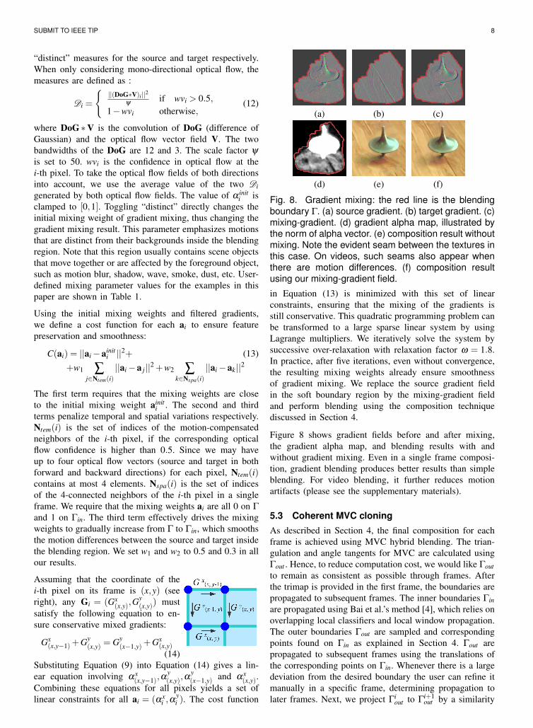
Fig. 8. Gradient mixing: the red line is the blendingboundary Γ. (a) source gradient. (b) target gradient. (c)mixing-gradient. (d) gradient alpha map, illustrated bythe norm of alpha vector. (e) composition result withoutmixing. Note the evident seam between the textures inthis case. On videos, such seams also appear whenthere are motion differences. (f) composition resultusing our mixing-gradient field.

in Equation (13) is minimized with this set of linearconstraints, ensuring that the mixing of the gradients isstill conservative. This quadratic programming problem canbe transformed to a large sparse linear system by usingLagrange multipliers. We iteratively solve the system bysuccessive over-relaxation with relaxation factor ω = 1.8.In practice, after five iterations, even without convergence,the resulting mixing weights already ensure smoothnessof gradient mixing. We replace the source gradient fieldin the soft boundary region by the mixing-gradient fieldand perform blending using the composition techniquediscussed in Section 4.

Figure 8 shows gradient fields before and after mixing,the gradient alpha map, and blending results with andwithout gradient mixing. Even in a single frame composi-tion, gradient blending produces better results than simpleblending. For video blending, it further reduces motionartifacts (please see the supplementary materials).

5.3 Coherent MVC cloningAs described in Section 4, the final composition for eachframe is achieved using MVC hybrid blending. The trian-gulation and angle tangents for MVC are calculated usingΓout . Hence, to reduce computation cost, we would like Γoutto remain as consistent as possible through frames. Afterthe trimap is provided in the first frame, the boundaries arepropagated to subsequent frames. The inner boundaries Γinare propagated using Bai et al.’s method [4], which relies onoverlapping local classifiers and local window propagation.The outer boundaries Γout are sampled and correspondingpoints found on Γin as explained in Section 4. Γout arepropagated to subsequent frames using the translations ofthe corresponding points on Γin. Whenever there is a largedeviation from the desired boundary the user can refine itmanually in a specific frame, determining propagation tolater frames. Next, we project Γi

out to Γi+1out by a similarity

SUBMIT TO IEEE TIP 9

transformation. If the union of projected boundary and Γi+1out

does not deviate too much (10%) from both boundaries,we use the union as the new Γout for both frames. Thisway, Γout is updated and clustered into several groupsover time. Within each group, the only differences in Γoutare a similarity transformation; the triangulation and angletangents are computed only once for each group.

To further reduce flickering, we smooth the membranevalue of MVC interpolation at the mesh vertices temporally.Our membrane may move together with the source object,unlike the fixed membrane used in Farbman 2009 [6].Therefore, instead of smoothing temporal neighbors as intheir paper, we smooth motion-compensated neighbors andmodify the smoothing weights of older frames accordingly.The smoothed vertex membrane value at frame i is calcu-lated as follow:

1W

[mi +2−d(i−1

∑j=i−5

(i− j)−0.75(||a||msj

i−1

∏k= j

wvsk + ||(1,1)−a||mt

j

i−1

∏k= j

wvtk)],

(15)where mi is the vertex membrane value before smoothing,and ms

j and mtj are membrane values of the motion-

compensated neighbors on frame j according to source andtarget optical flow respectively. a is the gradient mixingweight. wvs

k and wvtk are the optical flow confidences for

the source and target respectively at frame k. d is thenormalized distance to boundary Γ. W is the sum of weightsfor all m.

6 INTERACTIVE POSITIONING

Matching a source video object to a target video is challeng-ing not only because the scale, angle, position and lightingmust match in all frames, but also because the motionalong the frames must be consistent with the target videoscene. Our blending technique can compose source objectswith the background better, since it seamlessly transfersthe surroundings (e.g. shadows) of the transplanted object.However, it can still appear unrealistic if we do not positionthe object correctly.

We provide an interactive positioning interface to extendthe flexibility of our motion-aware composition framework.It has two main goals: to better align the motions of thesource and target videos, and more importantly, to allowfine tuning and editing of the motion of the source objecton the target video. We define the trajectory of the centerof the source object on the target frame as the object’smotion path. Our user interface design combines automaticcomputation with user interaction to reduce user effort andallow fast update with interactive feedback while editing.Towards this end we constrain the possible user edits tospecific points along the object’s motion path, and alsoconstrain the magnitude and orientation of possible velocitychanges. These manual changes are then automaticallypropagated to other frames. This prevents the creationof unnatural motion artifacts, and allows efficient localupdates. Combining interaction and computation providesan interactive-feedback system for easy motion refinementand editing.

6.1 Motion alignmentTo remove camera shake, we first stabilize the source andtarget videos using ideas from Zhang et al. [9]. This methodis based on a 3D perspective camera model, and formulatesthe stabilization problem as a quadratic cost function usingsmoothness and similarity constraints. Stabilization helpsthe subsequent video registration step. Zhang et al. [30]perform automatic metric reconstruction from long videosequences with varying focal length. We use their methodto recover the camera parameters and remove the cameramotion from both source and target videos. We removethe moving source object from the source video to preventoutliers. The user places the source object on the first frame,possibly with some rotation and scaling. The system calcu-lates a motion path for subsequent frames using automaticalignment. Trying to neutralize camera motion for all typesof complex video scenes is impractical, so we allow theuser to correct the position of the object on certain framesmanually.

6.2 Motion editingAfter automatic alignment and user refinement, good videocomposition results can be achieved. However, users maystill want to speed up, slow down, or change the trajectoryof the source object on the target frame. Such effects cannotbe achieved by simple composition with an aligned path:we support them via interactive motion editing.

Allowing arbitrary modifications to any point in the object’spath will break the intrinsic property of the motion path,causing artifacts to occur. Moreover, each time the path ischanged by the user, boundary optimization (Equation (7))and gradient mixing (Equation (13)) must be re-computed.This becomes a bottleneck for interactive update perfor-mance. In our boat example, MVC hybrid blending takesonly 1s, but these other computations take 6.6 seconds per100 frames. Hence, to prevent unnatural motion artifacts,and for efficiency, we intelligently constrain the editing ofthe motion path both to very specific points in time and topreset amounts.

The key idea is to explore both the motion propertiesof the object and the visual feature of the frames toobtain several control points, 2D points on the motionpath that indicate motion keyframes. We allow the user toedit only control points, and their modifications (includingtranslation, rotation and scale) are propagated to otherframes by linear interpolation. These points are optimalpoints for adjustment. The motion path is divided intoseveral segments based on two criteria: (i) the motion inone segment can be approximated by a uniform motion ina straight line, and (ii) the motion properties and visualfeatures should be stable at the control points.

Motion is quantified by speed, and visual features aremeasured by color mismatch across the blending boundaryas mentioned in Section 5. These two criteria allow us todetermine two properties: motion discontinuity at controlpoints, and stability of the control points themselves. We

SUBMIT TO IEEE TIP 10

greedily find n control points on the motion path byminimizing the following energy function:

En = µ1

n

∑i=1

(kti −kti−1 + kti+1

2)2 +µ2

n

∑i=1

−→vti2 +µ3

n−1

∑i=1

σ2i , (16)

where ti is the frame containing the i-th control point, ktiis the average color mismatch on the blending boundaryin frame ti, and −→vti is the object velocity in frame ti. Both||−→v || and k are normalized to [0,1]. σi is the variance of−→v inside the i-th segment of the motion path with controlpoints at the ends of the segment. We set µ1 = 0.2,µ2 = 0.2and µ3 = 0.6 in our experiments. Initially, the motion pathonly contains one segment, which means n = 2. The firsttwo terms of Equation (16) are set to zero whereas the lastterm is large. Next, we greedily find new control pointsuntil Equation (16) stops decreasing.

Using the control points, we divide the motion into severalsegments of approximate uniform straight line motion. Ifthe user edits the control point, these uniform motions arelargely preserved. In contrast, if modification is applied toan internal segment point, it will create a discontinuity.In addition, we impose local modification constraints onthe magnitude and orientation of velocity changes duringediting. These restrictions bound the area where the usercan change the path positions. When editing the k-th controlpoint, assume θi,θ

′i are the old and new orientation of the

i-th point’s velocity. If vi,v′i are its old and new magnitudes,then the restriction is:

∀i∈ [nk−1,nk+1],max(θ ′i −θi)2 < Tθ and max(v′i−vi)

2 < Tv(17)

To maintain the perspective continuity of the composition,we set Tθ = 30o and Tv = 20 as threshold values for all ourexamples. Figure 9 illustrates control-point-based motionediting.

Another key advantage of using control points lies inthe ability to apply only local updates and to interleaveinteraction with computation time. When the user edits thepath, we do not perform global optimization of Equation (7)and Equation (13) for the whole sequence. Instead, we cal-culate the blending results on segments which were changedpreviously but are not being edited. If previous calculationshave provided the boundary, mixing-gradient and MVCmembrane values on the end frames of these segments, theyare made hard constraints in the optimization. In summary,we interleave computation with user interaction to computeresults for other, non-edited parts. In our experiments,

t1

t2 t3

t4

t5

tn

Fig. 9. Interactive motion editing. t1, t2, ...tn are controlpoints on motion keyframes. Editing control points onlyaffects segments between locked control points.

editing one point requires 1-2 seconds, during which we cancompute 20-35 frames based on local optimization. Becauseof motion stability of the control points, and because thetemporal coherency restriction mainly utilizes informationin consecutive frames, we can merge several passes of localoptimization to approximate global optimization.

Compared with 3D Poisson blending, our algorithm allowsinteractive video editing both because of lower computa-tional complexity, and because of our control-point op-timization. While editing one particular frame, the usercan see the real-time result for just this frame via MVChybrid blending. Segments that are not yet calculated, arebeing calculated, and have been calculated are visualized indifferent colors (red, yellow and green respectively) on themotion path. The user can press a “play” button to instantlycheck video results using local optimization. The user canalso lock control points to avoid unnecessary re-calculationof already decided segments (see supplementary materialsfor examples).

7 EXPERIMENTAL RESULTSWe have tested our video composition system on severalchallenging examples and demonstrate the results in thepaper and accompanying video. Table 1 shows the gradientmixing parameters for each example. Figure 1(a) showsa slow motion hummingbird blended onto a stop-motionflower. The blending trimap for this example is shown inFigure 10(a). Our blending faithfully preserves the rapidmotion of the wing of the hummingbird and the water-drops. Figure 1(b) pastes a boat on the sea surface at sunset.The original source and target sequences contain severecamera shaking, and the water flow directions differ. Thewaves, reflections, and flag with the pole pose challengesto previous methods, yet are faithfully preserved, and themotion of the boat is natural due to interactive positioning.Figure 1(c) shows several planes blended into a cloud scene.Our method preserves the clouds between and throughthe planes and smoke without complicated matting. Theblending trimap is shown in Figure 10(c). Figure 1(d)shows a spinning top cloned to a different table. Ourmethod preserves the shadow and reflection of the spinningtop, while adjusting the texture to match the target table.Figure 1(e) is an interesting chase scene which pastesa snowmobile into a desert scene, chasing some goats.Figure 1(f) pastes a group of people diving into a fish tank,producing an interesting montage. The swimming fish inthe target video and the bubbles in the source video are

TABLE 1The gradient mixing parameters for each example.

Source Targetsalient base distinct salient base distinct

bird√ √ √ √

boat√ √ √ √

planes√ √ √

top√ √ √ √

snow√ √

dive√ √ √ √

SUBMIT TO IEEE TIP 11

(a)

(b)

(c)

(d)

Fig. 10. The input trimap and blending result. The user interaction strokes are shown in black and white. Pleasesee the accompanying video for the results.

both preserved without sudden disappearances thanks toour temporally coherent motion-aware blending technique.Figure 1(a) and (d) demonstrate that our blending methodcan deal with serious motion blur of source objects, Fig-ure 1(b), (c) and (e) demonstrate that our method is capableof preserving waves, smoke and dust effects in video. Ourmethod provides harmonious compositions with the targetenvironment.

Performance. All our experiments were performed on aPC with an i7 920 Quad core CPU and 12GB RAM.Preprocessing includes dense optical flow calculation, videosegmentation to decide the blending boundary type, andvideo stabilization (if necessary). Using our un-optimizedimplementation, these three steps typically take 5, 2 and2 minutes per 100 frames of VGA video. The user caninteractively draw the blending trimap and set the gradientmixing parameters. The number of needed user strokes forgenerating 100 frame trimaps is usually under 10, as we donot need to extract the boundary of the object. Next, thesystem generates an initial blending result for each framewith automatic alignment. With this initial blending, wealso save the vertex and angle information for MVC hybridblending. Then, the user can begin to interact for motionalignment refinement and motion editing.

Computation time and user interaction time for each stepare shown in Table 2. Interaction time includes time forgenerating trimaps and (optional) motion editing. Videoblending time indicates initial blending time and blendingupdate time in motion editing. The current frame blendingrate is achieved by utilizing two cores of CPU. Although itis approximately three times slower than the original MVCcloning method due to boundary optimization and distancescomputation, etc., it is still an order of magnitude fasterthan solving a Poisson equation as done in hybrid blending(using the TAUCS sparse linear solver). In practice, werestrict current frame blending to a single thread, and limitits rate to below 24 fps to save the computational powerfor segment blending optimization. Since our method usesapproximate MVC, we also show the RMS (root meansquare) differences of the hybrid blending results. Thesevalues indicate that the differences are unnoticeable. Us-

ing per-segment blending optimization produces additionaldifferences from the global optimization, which can bedistinguished, especially on motion keyframes. However,as long as temporal coherence is maintained between theseframes, blending results are still plausible.

Comparison. The supplementary video shows some com-parisons of our method to alpha blending using alpha mattegenerated by Bai et al.’s method [4], frame-by-frame hybridblending, 3D Poisson blending [23] and Xie’s method [24].Alpha matting loses many details around the source object,and the composition is unrealistic due to large illuminationdifferences. Xie’s method also loses details due to use ofmatting. We further compare the amount of interaction tothat needed by alpha matting in Table 2: alpha mattingusually requires 5-10 times more strokes than our method,even though the alpha mattes in those examples are stillnot optimal. Frame-by-frame blending and Xie’s methodproduce results which lack temporal coherence: flickeringon the boat and the wake are due to temporal fluctuationsin color mismatch, which are overcome by our blendingboundary optimization step. In frame-by-frame blendingand 3D Poisson blending, inconsistent motion along theblending boundary leads to a very noticeable seam; thisproblem is solved by gradient mixing in our approach.Our composition results are not affected by the artifactsmentioned above, and are also achieved at an interactiverate.

In Table 2 we summarize statistics and performance for theexamples in this paper. For single frame composition, ourMVC hybrid blending has higher quality than conventionalMVC [6] as evident in less color bleeding and texturesmudging, albeit at a cost of greater computation. For videocomposition, compared to matting based methods suchas [4] and [24], our method better preserves motion detailssuch as smoke, blurring and spray; compared to frame-by-frame hybrid blending and [24], our results displays bettertemporal coherence; compared to 3D Poisson blending [23],our method avoids visual seams around objects, and ismore flexible when the target video contains motion-salientobjects in the blending region.

Limitation. When the blending boundaries of the source

SUBMIT TO IEEE TIP 12

TABLE 2Performance of video composition.

frame number average cloned preprocessing interaction trimap matting video blending current frame MVC& frame size pixels per frame time(s) time(s) strokes strokes time(s) blending rate RMS

bird 115×1280×720 284,316 814 82 22 98 12.55 37 0.042boat 91×1280×720 182,405 855 127 7 43 6.64 88 0.037

planes 106×1440×1080 101,346 1,274 104 5 27 4.10 137 0.024top 82×330×300 37,762 65 25 4 39 0.93 211 0.018

snow 94×1280×720 220,818 902 93 8 137 9.56 49 0.029dive 297×1008×566 29,484 2,512 155 26 158 2.81 235 0.025

and target video sequences are very inconsistent, i.e. theirappearances and textures have large differences, our hybridblending based method degenerates to video matting, e.g.when compositing a white rabbit against a black wall.However, such cases are unsuitable for blending in thefirst place. Inconsistent lighting directions can also createunnatural blending results. This may be solved by illumi-nation estimation and relighting. Another limitation is thatour method cannot align video scenes with large camerarotation differences, since we are lacking 3D information.Since positioning is only applied in the image plane, it isunable to produce complex 3D object motion: for example,our editing tool cannot distinguish whether the snow mobileis jumping up or moving away from the screen. However,this could be improved by reconstructing a ground plane ofthe target scene and adding more degrees of freedom forpositioning. Our method also relies on various computervision techniques for pre-processing, and their imperfec-tions can also lead to artifacts. For example, although ourboat result vastly outperforms those generated by existingapproaches, one can still notice a blurred region on the deckof the boat. This is caused by inaccuracy of optical flow andits confidence values around the thin handrail of the boat.Adopting more recent advanced approaches like those inLiu et al. 2011 [31] may improve the results. Comparisonof different composition methods is also limited: thereis no reliable way to quantitatively evaluate compositionquality such as temporal consistency, apart from examiningthe results. Currently, such comparisons rely mostly onsubjective judgements or user studies.

Not every pair of video sequences is suitable for com-position. Large illumination differences, inconsistent back-ground environments and various motions of source object,camera, and background can all prevent good compositionresults. In fact, an added value of our approach is that weare able to give an approximate evaluation of the com-position quality by checking the consistency in differentsteps. For example, using hybrid blending, we can calculatethe composition cost, and after source object positioning,motion consistency could be easily determined. The accu-mulated score can suggest if the two video sequences can,in fact, be composed successfully.

8 CONCLUSIONWe have presented a novel video blending approach thattackles key challenges in video composition: complex ob-ject blending (smoke, water, dust) and motion differences.User-provided blending trimaps of the source video allow

us to create consistent blending boundaries over time. Wemix the gradients of the source and target videos inside theblending region, based on an efficient implementation ofmean-value coordinates interpolation instead of traditionalPoisson methods. We also provide a user interface toposition source objects and refine the results. All theseenable us to efficiently deal with complex video sequencesbeyond the capability of current solutions.

Our current implementation cannot generate the globallyoptimized video composition result in realtime; a possi-ble solution is to use a KD-tree to accelerate boundaryoptimization and gradient mixing. It would also be inter-esting to extend the method to more challenging results,for example, source objects that are moving towards oraway from the camera rather than primarily on a planeperpendicular to the camera. This would require moresophisticated user controls. To more faithfully recover theappearance of the source objects in the target video, betterillumination estimation could also provide guidance forgradient domain blending. Lastly, our user interface is stilllimited in versatility and accessibility, and it could beimproved by modern video editing techniques like thosein Chen et al. 2011 [32].

REFERENCES

[1] Y.-Y. Chuang, A. Agarwala, B. Curless, D. H. Salesin, and R. Szelis-ki, “Video matting of complex scenes,” ACM Transactions onGraphics, vol. 21, no. 3, pp. 243–248, July 2002.

[2] Y. Li, J. Sun, and H.-Y. Shum, “Video object cut and paste,” ACMTransactions on Graphics, vol. 24, no. 3, pp. 595–600, 2005.

[3] J. Wang, P. Bhat, R. A. Colburn, M. Agrawala, and M. F. Cohen,“Interactive video cutout,” ACM Transactions on Graphics, vol. 24,no. 3, pp. 585–594, Jul. 2005.

[4] X. Bai, J. Wang, D. Simons, and G. Sapiro, “Video snapcut: robustvideo object cutout using localized classifiers,” ACM Transactionson Graphics, vol. 28, no. 3, pp. 1–11, 2009.

[5] S.-K. Yeung, C.-K. Tang, M. S. Brown, and S. B. Kang, “Mattingand compositing of transparent and refractive objects,” ACM Trans-actions on Graphics, vol. 30, pp. 2:1–2:13, February 2011.

[6] Z. Farbman, G. Hoffer, Y. Lipman, D. Cohen-Or, and D. Lischinski,“Coordinates for instant image cloning,” ACM Transactions onGraphics, vol. 28, no. 3, p. 67, Aug. 2009.

[7] M. Grundmann, V. Kwatra, M. Han, and I. Essa, “Efficient hier-archical graph-based video segmentation,” in IEEE Conference onComputer Vision and Pattern Recognition (CVPR), 2010, pp. 2141–2148.

[8] M. Werlberger, T. Pock, and H. Bischof, “Motion estimation withnon-local total variation regularization,” in IEEE Conference onComputer Vision and Pattern Recognition (CVPR), 2010, pp. 2464–2471.

SUBMIT TO IEEE TIP 13

[9] G. Zhang, W. Hua, X. Qin, Y. Shao, and H. Bao, “Video stabilizationbased on a 3d perspective camera model,” The Visual Computer,vol. 25, pp. 997–1008, October 2009.

[10] Y. Boykov and M.-P. Jolly, “Interactive graph cuts for optimalboundary amp; region segmentation of objects in n-d images,” inIEEE International Conference on Computer Vision, vol. 1, 2001,pp. 105 –112 vol.1.

[11] C. Rother, V. Kolmogorov, and A. Blake, ““grabcut”: interactiveforeground extraction using iterated graph cuts,” ACM Transactionson Graphics, vol. 23, no. 3, pp. 309–314, 2004.

[12] T. Chen, M.-M. Cheng, P. Tan, A. Shamir, and S.-M. Hu, “S-ketch2photo: internet image montage,” ACM Transactions on Graph-ics, vol. 28, no. 5, pp. 124: 1–10, 2009.

[13] P. Bhat, C. L. Zitnick, M. Cohen, and B. Curless, “Gradientshop:A gradient-domain optimization framework for image and videofiltering,” ACM Transactions on Graphics, vol. 29, no. 2, pp. 1–14,2010.

[14] C. J. Armstrong, B. L. Price, and W. A. Barrett, “Interactivesegmentation of image volumes with live surface,” Computers &Graphics, vol. 31, no. 2, pp. 212–229, 2007.

[15] R.-F. Tong, Y. Zhang, and M. Ding, “Video brush: A novel interfacefor efficient video cutout,” Computer Graphics Forum, vol. 30, no. 7,pp. 2049–2057, 2011.

[16] Z. Tang, Z. Miao, Y. Wan, and D. Zhang, “Video matting via opacitypropagation,” The Visual Computer, vol. 28, pp. 47–61, 2012.

[17] P. J. Burt and E. H. Adelson, “A multiresolution spline with appli-cation to image mosaics,” ACM Transactions on Graphics, vol. 2,pp. 217–236, October 1983.

[18] P. Perez, M. Gangnet, and A. Blake, “Poisson image editing,” ACMTransactions on Graphics, vol. 22, no. 3, Jul. 2003.

[19] J. Jia, J. Sun, C.-K. Tang, and H.-Y. Shum, “Drag-and-drop pasting,”ACM Transactions on Graphics, vol. 25, no. 3, pp. 631–637, Jul.2006.

[20] Y. Zhang and R. Tong, “Environment-sensitive cloning in images,”The Visual Computer, vol. 27, pp. 739–748, 2011.

[21] P. Bhat, B. Curless, M. Cohen, and C. Zitnick, “Fourier analysisof the 2d screened poisson equation for gradient domain problems,”Proceedings of European Conference on Computer Vision (ECCV),pp. 114–128, 2008.

[22] M. Tao, M. Johnson, and S. Paris, “Error-tolerant image com-positing,” Proceedings of European Conference on Computer Vision(ECCV), pp. 31–44, 2010.

[23] H. Wang, R. Raskar, and N. Ahuja, “Seamless video editing,” inInternational Conference on Pattern Recognition (ICPR). Wash-ington, DC, USA: IEEE Computer Society, 2004, pp. 858–861.

[24] Z.-F. Xie, Y. Shen, L.-Z. Ma, and Z.-H. Chen, “Seamless video com-position using optimized mean-value cloning,” The Visual Computer,vol. 26, no. 6-8, pp. 1123–1134, 2010.

[25] J.-F. Lalonde, D. Hoiem, A. A. Efros, C. Rother, J. Winn, andA. Criminisi, “Photo clip art,” ACM Transactions on Graphics,vol. 26, no. 3, pp. 3:1–10, 2007.

[26] J. Lalonde, A. Efros, and S. Narasimhan, “Estimating natural il-lumination from a single outdoor image,” in IEEE InternationalConference on Computer Vision, 2009, pp. 183–190.

[27] K. Sunkavalli, M. K. Johnson, W. Matusik, and H. Pfister, “Multi-scale image harmonization,” ACM Transactions on Graphics, vol. 29,no. 4, pp. 125:1–125:10, 2010.

[28] S. Zhang, Q. Tong, S. Hu, and R. Martin, “Painting patches:Reducing flicker in painterly re-rendering of video,” Science ChinaInformation Sciences, vol. 54, pp. 2592–2601, 2011.

[29] A. Bousseau, F. Neyret, J. Thollot, and D. Salesin, “Video watercol-orization using bidirectional texture advection,” ACM Transactionson Graphics, vol. 26, July 2007.

[30] G. Zhang, X. Qin, W. Hua, T.-T. Wong, P.-A. Heng, and H. Bao,“Robust metric reconstruction from challenging video sequences,”in IEEE Conference on Computer Vision and Pattern Recognition(CVPR), 2007, pp. 1 –8.

[31] F. Liu, M. Gleicher, J. Wang, H. Jin, and A. Agarwala, “Subspacevideo stabilization,” ACM Transactions on Graphics, vol. 30, pp.4:1–4:10, February 2011.

[32] J. Chen, S. Paris, J. Wang, W. Matusik, M. Cohen, and F. Du-rand, “The video mesh: A data structure for image-based three-dimensional video editing,” in IEEE International Conference onComputational Photography (ICCP), april 2011, pp. 1 –8.

Tao Chen received the BS degree in Funda-mental Science Class and the PhD degree incomputer science from Tsinghua Universityin 2005 and 2011 respectively. He is cur-rently a postdoctoral researcher in Depart-ment of Computer Science and Technology,Tsinghua University, Beijing. His research in-terests include computer graphics, computervision and image/video composition. He re-ceived the Netexplorateur Internet InventionAward of the World in 2009, and China Com-

puter Federation Best Dissertation Award in 2011.

Jun-Yan Zhu received the BE degree withhonors in computer science and technologyfrom Tsinghua University in 2012. He is cur-rently a PhD student in the Computer Sci-ence Department at Carnegie Mellon Univer-sity. His research interests include computervision, computer graphics and computationalphotography.

Ariel Shamir is an associate Professor atthe school of Computer Science at the Inter-disciplinary Center in Israel. Prof. Shamir re-ceived his Ph.D. in computer science in 2000from the Hebrew University in Jerusalem. Hespent two years at the center for computa-tional visualization at the University of Texasin Austin. During 2006 he held the positionof visiting scientist at Mitsubishi Electric Re-search Labs in Cambridge MA. Prof. Shamirhe has numerous publications in journals and

international refereed conferences, he has a broad commercial ex-perience working with and consulting numerous companies. He is amember of the ACM SIGGRAPH, IEEE Computer and Eurographicssocieties.

Shi-Min Hu received the PhD degree fromZhejiang University in 1996. He is current-ly a professor in the Department of Com-puter Science and Technology at TsinghuaUniversity, Beijing. His research interestsinclude digital geometry processing, videoprocessing, rendering, computer animation,and computer-aided geometric design. Heis associate Editor-in-Chief of The VisualComputer, and on the editorial boards ofComputer-Aided Design and Computer &

Graphics. He is a member of the IEEE and ACM.