Submitted to Physical Review D LBL- 543

A GENERALIZED

David J. Herndon, Paul Soding and Roger J. Cashmore

SLAC Pub- 1385 Preprint

IS’OBAR MODEL FORMALISM

L-

July 1973

Prepared for the U. S. Atomic Energy Commission under Contract W-7405-ENG-48

-iii- LBL- 543

A GENERALIZED ISOBAR MODEL FORMALISM* 4.

David J. HerndonT and PaulS6dingS

Lawrence Berkeley-Laboratory University of California

Berkeley, California 94720

and

Roger J. Cashmore 5

Stanford Linear Accelerator Center Stanford, California

ABSTRACT

We present an isobar model formalism for analysing the re-

action a t b --* 1 + 2 + 3. Arbitrary spins are allowed for all the

particles. Polarized particles and weak decays of an outgoing

particle are discussed. We also show how to extend the formalism

to allow an isobar analysis of a three-body subsystem of an n-

particle final state.

Work done under the auspices of the U.S. Atomic Energy Commission.

-l-

INTRODUCTION

- In this paper we discuss a general formalism for analysing reac-

tions of the form

atbdlfZt3

using the Isobar Model. Previous work has either specialized to the

case of srN + N’ITIT I-9 or only covers parts of the formalism. 10-12

Our formalism is completely general in that it allows arbitrary spins

for all the particles. The formalism was developed for an analysis of

TTN --L Nrrn data, 13

which appears as a companion paper.

In Section I we establish our notation and normalization of states,

review the angular momentum decomposition of two-particle states t

and develop formulae for phase space and differential cross sections.

Section II deals with the T-matrix elements themselves and derives the

equations for the differential and total cross sections. Section III deals

with polarized particles, either incident or final, and with weak decays

of an outgoing particle. Section IV treats the problem of analysing a

three-body subsystem of an n-body final state. The appendices include

a review of angular momentum, a discussion of the reaction

atb+ c t d using our notation, and the details of some of the more

important derivations.

SECTION I

In this section we establish our notation. We consider the reaction

atb+ 1 t 2 t 3, where a is the beam, b the target, and 1,2,3 are

the three outgoing particles. We let j, k, and 1 represent any cyclic

permutation of 1) 2, and 3. The diparticle is always composed of

particles k and 1. All quantities pertaining to the diparticle are indexed

by a subscript j. The following quantities are summarized in Fig. 1.

a. Total CMS energy and angular momentum - W, J

b. CMS four-momenta - pa pb Qj Qk Q,

-2-

c. Particle spins - cr a 0 0. (7 Q b J k 1

d. CMS helicities - ~J.a ~b CLj ok IJ.1

e. -Mass of diparticle - w. J

f. Spin and CMS helicity of the diparticle - j. X. 3 3

g. Incident orbital angular momentum and total spin - L, S

h. Outgoing orbital angular momentum and total spin - L ., S. 3 .I

In the diparticle rest-frame we have the quantities

i. Four-momenta of the decay particles - qk q1

5 Helicities of the decay particles - vk v1

k. Orbital angular momentum and total spin of decay particles -

1 ‘, 3 7’

Angular momenta are coupled in the following manner:

We assume that L, L., 3

and lj are chosen so as to conserve parity. We

use p to represent a fixed set (p., +, pj pk cl,) of all five helicities. For

simplification in later sections, n represents the set of quantities

n, = (j; J; L S; Lj Sj; jj lj sj)$ ($1

where j specifies the grouping of the final-state particles into a single

one (j) and the pair (kl).

We use the helicity formalism with the phase convention of Jacob

and Wicki (hereafter called JW).

-3-

Particle States, Phase Spaces, and Cross Sections

- One-particle states are defined with the phase convention of JW al-

though the normalization is different. If q PA

represents a state with

momentum P along the z axis and helicity X, then the general state is

defined by [ cf. JW Eq. (6)]

/ :A > = /p ‘3-b A) = R(+,@, -+) qpxa (2)

We choose the normalization to be

(pIeI 91, A’ / pe+,x) = 2m3@ -i;pAA, , (3)

which differs from JW by the factor 2E/(2~)~. We also define states

XpX bY

xpx = (-1) s-x R(O,r,o)$ -PA

= (-WA $+.

The general x state is given by

j -;A) = 1 -p@+,X) = R(+,@, -o)xpi . (5)

We shall denote these states by the minus sign on p. Thus

/-pew4 = C-1) S-A,

ip T-8 (p tTT,x). (61

Clearly these states have the same normalization as 1 p&$,X ) .

We also need to know how the states /pe$,X) transform under

Lorentz transformations. Let the Lorentz transformation be 1, where

P’ = Ip and let U(1) be the unitary operator for 1. Wick” has shown

that ( U(l) 1 pe4bx) = F I$, (Qa> 1 p’e’+‘,v )-, (7)

where 52 is called the Wigner angle and Fi is a unit vector along

p”’ X p’ if 52 is always taken to be positive. This is clear, since in

the transformation the momentum vector makes a positive rotation

around the direction p”X $ and the spin lags behind, thus making a

negative rotation with respect to the momentum vector. We discuss

fi in detail in a later section,

-4-

Multiparticle states are defined as the direct product of one-particle

states. Thus

~j&,~2h2’. * * ,; nAn) = / plel~,~~, ) j ~~~~~~~~~~~~ e I pnen+nSAnl (6

and

3-T = ’ (2Ei) ’ (pi -i;i, ‘A A’ .

i i i

For two-body states it is sometimes more convenient to use the vari-

able s

G= Cl ts2,

g= $6, - F2) * Letting (PO+) be the polar coordinates of $, we have

with the states on the right-hand side either Q or x states. These

states are normalized such that

‘Al A; ‘A2Af2 = i

d3 d3 (FYpfewxfl~~2 j Es,pe+,AlA2) -&++ &f .

Now d3pld3p2 = d3Pd3p = d3P p2dpd2a, where d2 w = dcos Od+

is the total energy, W = E1 t E2, then

dW = [W t B.;i”:-“l)]& .

With these two relations it is easy to show that the normalization is

-5-

In the center of mass system, P = 0, so this reduces to

(15)

To discuss the decomposition of the two-particle states into angular

momentum states, we work in the two-particle center of mass and

assume particle 2 to be in an x state. For this case, using Eq. (II),

we have

iP = O,~e+,x,x,) = Ip?ii ) 1 -32j = R(+,e,-+j+phlXpX . 2

(16)

We now define a state of total angular momentum J and z-component

/P = 0, pm, Xl12 ) = NJ /

D~A(~,e,-~)lB=o,pe~,x,-x,) d2w, (17)

where X = X1 -X2. Using Eq. 15 and the normalization properties of

the D-functions, we have

($I = O,p’J’M’, X;h; 1 3 = O,pJM, X1x2 )

* 4?T 4w 6 = NJNJ 2J-H p JJ’%dA A”h A’

63(-Pe)6(w’-w), 11 22

where W is the total CMS energy. Thus we choose

’ NJ = (2J4; I” l/l(&) li2. (19)

The factor (p/4W) 1’2 [cf. JW Eq. (22)] comes from our choice of

normalization for the one-particle states. Using Eq. (f7), the trans-

formation matrix is

-6-

In terms of the orbital and spin angular momentum, L and S, we have

the standard expansion:

/p’= O,pJM>LS )

S S 1’ 2’ j Ai’ -A2) C(L, S, J j 0, X1-X2) (2

13 = O,pJM, XIX2 ),

with the normalization

(p”= O,p’J’M’,L’S’I F = O,pJM,LS )= dJJ,6MM,bLL,~ss,6?(~‘-~~6(W!-W)

(22)

Ifparticle 1 is a photon, one instead usually uses the multipole

expansion

is = o,pJM,j~ ) (2la)

112 (-lJe C(j, S2, J / X1, -x,)/is = O,pJM, X1X2 ),

where the total (spin plus orbital) angular momentum and parity of the

photon are j and TI = (-i)j*respectively, For e = 0, we have the elec-

tric 2j -pole and for e = 1, we have the magnetic 2’-pole, These states

are normalized such that

(gl= O,p’J’M’, j’r’ / 3 = 0, pJM, jr) = 6 6 JJf’MMr6jjf TT’TF’ h3(Pl -$)6(W’-W).

122a)

In-the rest of this section wedeal indetailwith the numericalfactors

appearing in cross-section formulae. The normalization, Eqs. (3) and

(IO)* are such that the number of particles of type i in a volume V is

-7-

2EiV/(2~)3. In a volume V the total number of states available is

T d3pi/(2n)3, SO that the density of final states per particle is d3pi/2E.. 1

Thus the number of three-particle final states available, dpF, is given

bY

(23)

The probability of transition (in all space and time, Vt -03 ) is given by

I b4(Pout - Pin)M / ‘dpF’ (24)

where M is the transition matrix element with our normalization of

states, i. e., M = (out IT I in). The relation with the S-matrix is

(out 1 S j in) = bout, in t i h4(Pout-Pin) (out 1 T 1 in ) .

Equation 24 then gives

I b4(Pout -Pin)M I2 = ;y+ o. % 64(Pout-Pin) 1 M / 2 (27.r)

so that the transition probability per unit volume per unit time is

(2+464tPout-Pin) / M / 2dpF -

With the normalization of Eq. 3, the incident flux is

(25)

(24)

(27)

(28)

2 2 112 where F is the invariant flux factor and F =[ (pa. pb)2-maml] .

In the CMS, F I= pW.

The density of final states dpF together with the h4 function of

Eq. (27) give

dp = “(Pout-Pin)dPF. (29)

Berman and Jacob 15

have discussed this phase space and reduced it to

dp = $ dE1 dE2 dcosO d$ da (30)

where 0,3, and (Y are the Euler angles specifying the orientation of the

-8-

final three-particle state with respect to the incident system. Equation

(30) canbe further manipulated to give

-h 1 91Qi

dp= - 8 2WWl

dw; dcosel dcosO dq, dcr (312)

1 91Qi = - 8

- dwl dc.osei dcos0.d$ dcu W. (31b)

= $ (4W2)-1 dw: dw; dcosQ d$ dcr, (31c)

where w 1 i’s the invariant mass of particles 2 and 3, and e1 is the angle

between particles 1 and 2 in the (23) CMS, Q, is the momentum of

particle 1 in the (123) CMS, and q1 is the momentum of particle 2 or 3

in the (23) rest frame.

The differential cross section for the case of spinless particles is

do =$- 2 IM12dp,

which is the basic expression we use in the calculation of our formulae.

SECTION II

Initially we discuss the reaction proceeding through just one inter-

mediate isobar, i. e. , j is always fixed at a certain value of 1 t 2, or 3.

Later we treat the case of more than one type of diparticle.

In terms of the transition operator, T, the matrix elements in the

center of mass are

The operator T is assumed to be the product of a production operator

Tp and a decay operator Td. Assuming that only two-body intermediate

states are produced, we have

2En63’am -+ dn,

(33)

-9-

Within the Isobar Model one assumes that the intermediate state con-

sf‘sts of an isobar state recoiling against a single particle and that T d

operates only on the isobar state, therefore

(35)

SO that Eq. (33) becomes

(36)

We have assumed the isobar to be in an x state [ cf. Eq. (5)] and have

changed the isobar helicity to 1.. 3

One term represents the production

of the isobar and particle j; the other term represents the decay of the

isobar into particles k and 1. We now discuss each term separately.

Production Amplitude

Since we have assumed the diparticle to be in an x state, we use

Eq. (20) to decompose both lFa~a, gbpb j and (Bjpj, -tijXj I into angular

momentum state s. We have

x (~ = o,ajJM,CljXj ITpIP = O,PJM,~~~~).

Since we have not as yet specified a coordinate system, we do not give

angles as arguments of the D-functions. We will return to this point

later. Using Eq. (7) from Appendix A and converting from helicity

states to LS states, we have

-lO-

(38)

x C(aa,ob,S /pa, -pb) c!L, s, J / 0, pa-b)

X C(Oj9jj,Sj I 'lj' -hj) G(Lj, Sj, j/ 0, t+;) J

X DJ ~j-'j r”a-~

(j-l beam)

X (i3 = 0, QjJ”, LjSj 1 Tp 1 fs = 0, pJM, LS) .

If particle a is a photon, instead of converting to LS states, one would

prefer to couple to the multipole states defined in Section I. We may

now use rotational invariance to write the reduced partial wave produc-

tion matrix element as

(a = O,QjJM,LjSjl TpjY = O,pJM,LS) = T;l& s tW,wj) .

“j j

Decay Amplitude

-The decay amplitude is most easily evaluated in the rest frame of the

diparticle. We use Eq. (‘7) to transform the states. Recalling that the

diparticle is in a x state, its transformation is quite simple. (While

the X state reduces to a simple form in its rest frame, it also implies

a fixed direction for the z-axis, along the direction a’. in this frame. J

The decay angles ej and (pj are then the angles of qk in this coordinate

system; i. e. , only +. is unspecified, J

since the x and y axes are not

yet defined. ) Thus

=C D Uk *

(e%i )D a1 :::

‘kVl ‘k Pk (eta ) (<

J k v1 Pl J 1 kvk’<lvl 1 Td 1 jj - ‘j) * (40)

Using Eq. (4) to convert the states of particle 1 to x states, we can

then insert an angular momentum decomposition. Converting to an LS

representation, we have

3 kV1

(Zlj f I)~‘~ C(U~,U~* sj 1 Vk’-vl) C(lja ‘j’jj 1’3 ‘k-‘l)

Jj ~ al- vl XD-A v (41)

j kWV1 (decay) D Ok” (ek$)

‘k Pk J

X (T = 0, qkjj-Xj, ljsj ITd( jj-Xj) .

The reduced decay matrix element is then just a function of w., 3

(a= O,qkjj - Ajsljsj ! Td / jj - Xj ) = B:’ s (wj).

j j

Recalling the definition of n in Eq. (1) and combining equations 38, 39,

41, and 42 (remember that p stands for the set pa ‘43 pj pk pl), we see

that f can be written as P

fp = g g:(j) T,(W~Wj)r

where Jj.

T,(W, wj) = ‘j TLdL s (W,wj) B1 i j

s (Wj) j j

and 112

[ (2L t I) (2Lj t 1) (21j t I,] 1’2

(43)

(44)

X C(o a’ ab, S 1 pa, -t-jJW, S, J 10, ~~-t+,,)

(Eq. 45 continued)

-12-

XAT C(aj, jjaS. / pj9 !

Aj)C(Lj, Sj’ J 1 0, Pj-hj) DJ -x p - (I-lbeamj

I- ‘j ja% (45)

XX C(G~, G 1’ ‘j / Vks -vl)Cllj 9 sj9 jj / Qs Vk-Vlf dj tic VkV1 -3 ‘kmV1

(decay)

XD Gk :k “1 le.

($kC ) D >::

vlPl’ejnl) ‘-I) al-v1

* vkpk J k

Although it is included in n, we have explicitly written the type of iso-

bar with gz. Since the isobar quantum numbers are included in n,

Eq. (43) is valid when there are more than one j-type isobar.

Up to this point we have made no mention of a coordinate system and

our formulae are completely general. Some simplification occurs with

various choices of axes. We choose the Y-axis to be the normal to the

three -particle plane. (Another common choice is to take the Z -axis as

the normal to the three-particle plane. )

~:djXi3k=$xdl=qx~j~ (46)

In the case of the Isobar Model it is then convenient to choose the Z-axis

as a polar vector in the three-particle plane. We ckzoose Z along8. S The J

polar angles of the beam are @ and Q , while the particles j, k, and 1 have polar

angles (Oj, sj), (8 k, $,,, and (8,, $,) respectively in the CMS. With our

choice of axes it is clear that Gj, Qk, alare either 0 or n and $ = 0. These

angles are summarized in Fig. 2. In this case we also have

8, = - $$ = ?. For, convenience we introduce the angles aj, pj, y j, where

R(aj, pj’,yj) = R(j-’ beam) = R(gj9 -ej, - ipj)R($,O,- *). (47)

We then have the following simplifications in the expression for g’: n

-13-

j. *

-D-Jx. v J k-‘1

(dec.ay) -+ d’j -xj Vk-vl tej!’

(48)

G, *c D1

7 iJ;l (6h,) -t d*’

J y $q *

At this time we can now consider the angles 5; and C3: . Wick’* dis-

cusses these angles in detail and shows that

coser = (coshp - cash akcosh 0;) / (sinhok sir&Q,

(49)

c0sej. = .I t

COS~P - cOShrJ1 cash 0-i j / (Sid2 G1 SinhGi) ,

where

tanh p = -2 = velocity of j in CMS,

tanh gk= vk = velocity of k in CMS,

tar&ok= vk= velocity of k in fkl) rest frame,

with similar equations for 1, We want to further clarify the sign of the

rotation angles. Figure 3 illustrates the effects of the ,Lorentz transfor-

mation in a non-Euclidean plane. Remembering that the spin lags be-

hind the momenkum during a Lorentz transformation, one sees that for

particle k a positiva i rotation about the Y-axis is needed, and for par-

ticle 1 a negative rotation about the Y-axis (corresponding to $ = -7

above. ) We understand $and $are always positive in Eqs. (48) and

(49). In terms of the Stapp $6 angle 52 the Wigner angles are

(50)

-14-

i where 0

kj and 8

lj are the CMS angles between z. and Q,,

J 5, re-

spectively.

The-Reduced Production and Decay Transition Matrix Elements

We now look at the function T in more detail. T as defined in n n

Eq. (44) is composed o1 $ two factors and we consider each separately.

Production Matrix Element

The first factor T j is the production amplitude. For

convenience near threshoid’one can explicitly write the barrier pene -

tration factors 17

t4w) -l/Z pL t (l/2) t4w) -l/2 QLjt(1’2i j . (51)

The charge dependence is also removed by including the isospin vector

addition coefficients. Thus

Jj , TL~L S.(w, wj)

j 3 pL + (1/2JaLj

= 3 4w

.Ti

‘2’

where T ILL S.(w’wj ) is a function slowly varying in w.,

j J 3

Ia and I”, are the i sospin and z-component of isospin for a, I b % ana

I,” are the isospin and z-component of isospin for b, IJ and Ij are the Z

’ D isospin and z-component of isospin for j, I

D and Iz are the isospin and

z-component of isospin for the isobar, and I is the total isospin.

Further explicit dependence on W or wj can be introduced as factors in Jj.

7L~L.S (w’ wj)’

One popular choice is a form factor of the form J j

(1 t R’Q;, -Lj/z

, 153)

which includes a radius of interaction R.

Decay Matrix Element -

4 Taking the charge dependence out of the decay term we have

(54)

where we have used the same notation as before. j.

To evaluate A:.s (w’.) one ‘uses eithe, ?- the Watson final-state interaction 4&j ’

theorem or a modified Breit-Wigner function. Using the Watson the-

orem, one takes l/2

911 ‘, 4”j/!’ p (55)

where 6 is the elastic scattering phase shift at the mass w.. We J

have added the extra factor (q,/dwJ) f/2 to ensure the proper threshold

behavior in our normalization. With Breit-Wigners one may choose

either the relativistic or nonrelativistic form. For the relativistic case

one uses

where

r.(W.j = S.(w,) J J J

(56)

and w. is the resonance mass. Jackson al

has given a discussion of

the different for’ms for p(w). For the nonrelativistic case one uses

-f/2

[ r . (w.) /Z ] u2

(2TWo) (w. -wj)-iTj (wj)/2 ’

where I’.(w.) is defined as before. Both of these forms are defined J I

such that in the limit of zero width we ‘nave

(59)

-16-

Cross Sections and Threshold Dependence

We are still considering just one diparticie pair (k1!, but there may c,

still be multiple isobars in this system. From Eq. 32

the differential cross section is, for unpolarized incident particles

and without observing the polarizations of the final particles,

2 da=+- ~ p’ Z /f I2 dp,

where

z = [ I20,4- 1) j2Ub -t I)] --I 2 .

(SO i

Since we are concerned with unpolarized cross sections, we may inte-

grate over cy (the angle of rotation about the incident beam) in Eq. (31a)

to give rrqkQ*

dp = & dwj? dcos ej dcos 8 d$ . J

162)

The total cross section then becomes

: ,k -i-rq Q. F $&.$;g; k

I Tn!W,wj)Tm(W,wj) 8w ~- j

dw; dcos “j dcosO d$,

This expression can then be reduced (as in Appendix Cj to give

i j T (W,w.) j n 3

!2 dw;. (64)

We note that isobars of different quantum numbers in the jkl) subsystem

do not interfere. ’

If we now use a Breit-Wigner form for AJj s (wj) and take the limit j j

as l?.(w.) + 0, the cross section reduces to J J

Since in this limit the diparticle has become a stable particle, this

-I?-

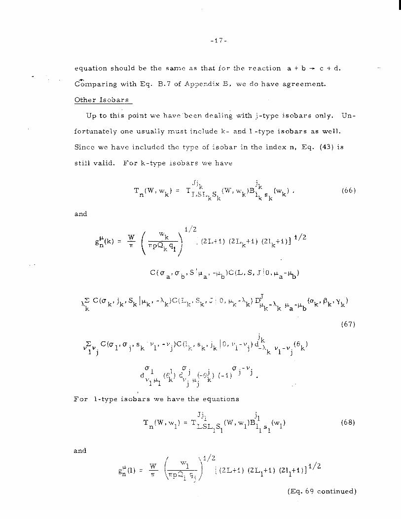
equation should be the same as that for the reaction a t b + c t d.

C;mparing with Eq. B.7 of Appendix B, -we do have agreement.

Other Isobars

Up to this point we hav e’been dealing with j-type isobars only. Un-

fortunately one usually must include k- and 1 -type isobars as well.

Since we have included the type of isobar in the index n, Eq. (43) is

still valid. For k-type isobars we have

J;

Tn(W,Wk) = $& s “k k

(W, wkiB~ks (w,) . k k

and

a’ -i$)c(LS s, J 10, p a -%)

(66)

k, j,, Sk jpk, -XkjC(Lk, Sk, Z I 0, ‘*k-Xk) DJ pk-‘k tL,-IJ.b bk* P,, v,)

(67)

jk v~ym C(o190 ., sk / vl, -vjiCjlkn skz j, j 0, ~~l-vq) dmx

1 J 3 4 k V1-“j

(Ok)

For l-type isobars we have the equations

JJ, T,(W, wI) = T

Jl L;L,Sl~w~wl)Bll SICW1)

/

and

(68)

(Eq. 69 continued)

-18-

z jl

‘jvk C(0 j’ Ok’ si I v:,

J -vk)Ctlls si, j, 1 02 Vl-Vj)d_x v -v

lj k CO11

In each case we have preserved the cyclic order of j, k, and 1. The

total transition amplitude in the case of more than one subsystem con-

taining isobars is then written as before:

fP = 22 g: (j) Tn(W, wj). jn

(43)

This coherent addition implies some double counting of the amplitudes

which has, in practical situations, been shown to be small. 18

In the case when there are identical particles presen&care has to be

taken to ensure that one uses a correctly symmetrized combination in

Eq. 43. Our cyclic ordering of the particles j, k, and 1 will not neces-

sarily ensure this and this has to be explicitly introduced.

Symmetry Properties of the Amplitudes

We next discuss the symmetry properties of gP under certain cir- n

cumstances.

Consider the case of p* - EL, the result which occurs under Parity:

the operation of parity. In Appendix D we show that

g-p = q(-1) ‘asPa (-1)

“b-“b akiiJk&+ ‘tigp * (70) n n ’

where n is the product of all five parities. For any specific problem

this reduces the number of independent g,“. For the case of TIN+NSTTT,

‘1% - 1 and we have

gp % n ’ (71)

where pi is the incident nucleon helicity and /of is the final nucleon

helicity. Since T n is independent of Jo, we have

f .-P =$ g-pT n *?

=~gi.l”T n n’ (72)

Interchange of two particles: We may also discuss the properties of

our amplitudes g: (w;, WC, 2

w, ) under the interchange of two particles

k and 1. Such a change is relevant for discussion of symmetry proper-

ties in the presence of two identical particles.

In our’formalism a cyclic order is always preserved and thus inter-

changing k and 1 leads to a change in the coordinate system, “ye 3.

Associated with this, we have the changes

(73)

We find that (see Appendix E) for j-t-ype isobars,

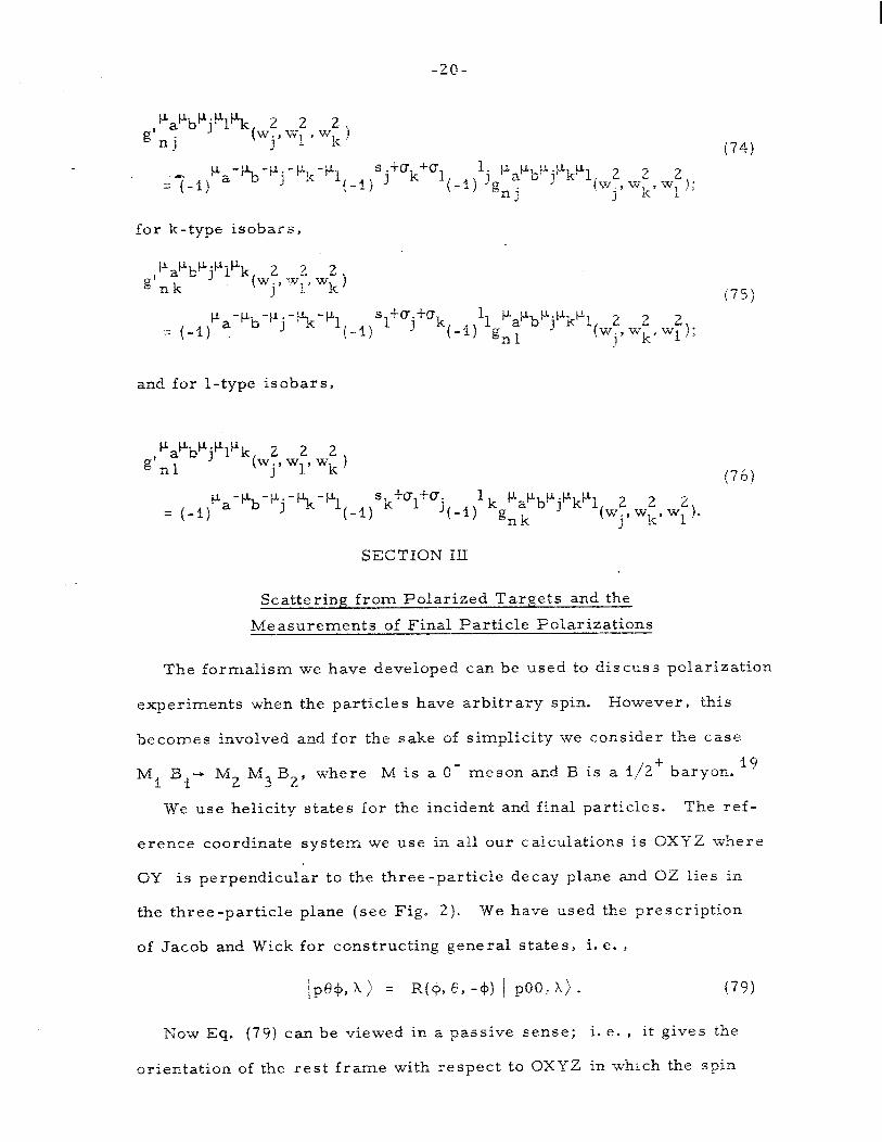
-2o-

%ILbPjPIPk 2 2 2 g’nj

(Wj’W1 ‘Wk! (74)

=+(-I) Pa-%b-Pj-?k-‘lt -1 )’ j+ak’ol( \

1 )‘jePaPbsjPku11;2, w2, w2 .~. -i -‘n j J k 1,’

for k-type isobars,

Pa’b’jPIPk( 2 2 2 g’nk w . , “xi , w

J 1 k)

and for l-type isobars,

(76)

= (-1) ‘Sa-‘Lb-Pj-%-Pl(-i) ’ kt*ltoj ( _ 1 \

I 1 kgPaPbP j’k’l(w,!, 2

nk 3 2 )

Wk’W1 *

SECTION III

Scattering from Polarized Targets and the

Measurements of Final Particle Polarizations

The formalism we have developed can be used to discuss polarization

experiments when the particles have arbitrary spin. However, this

becomes involved and for the sake of simplicity we consider the case

Ma E$-” M2 M3 B2’

where M is a O- meson and B is a I/2’ baryon. 19

We use helicity states for the incident and final particles. The ref-

erence coordinate system we use in all our calculations is OXYZ where

OY is perpendicular to the three-particle decay plane and 0Z lies in

the three-particle plane (see Fig. 2). We have used the prescription

of Jacob and Wick for constructing general states, i. e. ,

(79)

NOW Eq. (‘79) can be viewed in a passive sense; i. e. , it gives the

orientation of the rest frame with respect to QXYZ in which the soin

-21-

components X are defined. This rest frame is obtained from OXYZ by

tze operation R(+,6, -$I). These final coordinate axes are then the

helicity frame axes. These are described in Fig. 4 and we see that the

particle has spin ‘component X along CZ”’ in the coordinate system

Qx'ilylllzll' I)

Final Particle Coordinate Sys terns : For our final particles the

helicity frame axes are defined by

OZ’ =

oy’ =

OX’ =

(80)

and are demonstrated in Fig. 5.

Initial State Coordinate System: Ln this case the helicities are de-

fined in a rest frame OXIYIZ19 which is obtained from OXYZ by rotation

through the Euler angles $,8, -9; thus9 OZi is along the incident mo-

:I: 2 I? t1J.m ; - a’

Now, if we use a polarized target, then we define a very

specific initial coordinate system. Let this coordinate system be

Oxyz with Oz along Fae Then Oxyz is related to OXIYIZl by a rotation

CY around the OZ1 axis. We have the following relations between co-

ordinate frames:

OXYZ - OXIYIZ1 Euler angles $,O, -$,

OXIYiZl - oxyz Euler angles O,.O, cy, f8f)

OXYZ + oxyz Euler angles $, 0, CY-$ .

Transition Matrix Elements: We have calculated transition matrix

elements from initial states defined in the frame OXIYIZ1, whereas we

require transitions from states defined in Oxyz to discuss scattering

from polarized targets. If A P

is the amplitude for transition from

OXiYiZi and AL is the transition amplitude from Oxyz, then

-22-

-i+ AL = Ati e

a-tjJQ (82,)

If we-onsider only the reactions of the type TTN-+ Nnv,then Eq. (82) re-

PolarizBtion Experiments: We assume we have a coordinate system

Oxyz in which the initial polarizatioc is specified and the r’inal baryon

polarization is described in the helicity frame.

a) Unpolarized cross sections: The initial density matrix is -

PI = (lj2)T The differential cross section is then written as

b) Polarized target: - if----q

The initial density matrix is now pi = 21 1 t Pbud

We then have a differential cross section

w ’ ‘b ._ e r e is the polarization vector of particle b in the Oxyz frame.

c) Final Polarization (of Particle 1’;: -i

Here I p = (i/sj-TzCG’, where

T 0

Trace (p ) = 1. The final baryon polarization is given by

(86)

d) Depolarization Tensor: For final polarization from a polarized

target we have

(87)

7 where Trace (p ) = 1. The component of spin of particle 1 along an Avis

M (=X, Y, or Z) is PIM and is given by

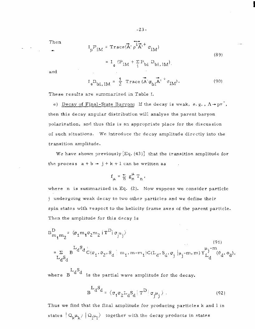
-23-

Then

c,

-

IP i-P -4

P ml = Trace(X’ p A’ cJIM)

and

‘oDbi LM = + t

, $ Trace (Zl~biA’ “1M) *

(89,

(90)

These results are summarized in Table I.

e) Decav of Final-State Baryon: If the decay is weak, e. g. , A-tpn-,

then this decay angular distribution will analyse the parent baryon

polarization, and thus this is an appropriate place for the discussion

of such situations. We introduce the decay amplitude directly into the

transition amplitude.

We have shown previously [Eq. (43)] that the transition amplitude for

the process a t b - j t k t 1 can be written as .

fp =

z g,” Tn’

where n is summarized in Eq. (2). Now suppose we consider particle

j undergoing weak decay to two other particles and we define their

spin states with respect to the helicity frame axes of the parent particle.

Then the amplitude for this decay is

BD mlmZ= bimi02”2 / TD/ ajpj)

LdSd i P.-m =z B

=dSd

C(CJ?, CT,, Sd j ml, m-ml!C(Ld, Sd9 G. /pj-m, m) YL L J d t6ds +,h

where B LdSd

is the partial wave amplitude for the decay.

B=dSd = (ol”zLdSd / To j ojvj > . (92)

Thus we find that the final amplitude for producing particles k and 1 in

states I; Qk’Lk’ / Q,t$

together with the decay products in states

:ame .axze s of Darticie j A

In the case of A decay obtaiPred, for ia.stance, in the reaction

many simplificatiox2s result, :J2 = 0 i m:, x 9, arLd we have bl

a specific initial c65xdinate system, iThen

6943

sEc.~y-,r?- "TJ .a.* I i

Analysis of Three-body States Ob~aine d in Prc~duction Reactions -II_

Another fruitf& area for appIlc.ation of the formalism we have de-

veloped is in the study of three-partizie states formed in production

experim.ents. We are particularly concerned with reactions of the type

-25-

GA which there are many examples being studied at present, e. g. ,

v + p -+ p f (A1,A2,A3)’

k+p- p C iQ,.Lj, 198)

T(k) t p - r(k) t N*.

We now develop the slight changes necessary to deal with these reac-

tions. -We use a notation essentially the same as that described in

Section I. The only modifications are:

a) We have to define the quantities pertaining to the extra particle c.

We use

% - intrinsic spin Gf c,

% - helicity of c,

PC - four-momentum of c.

b) All quantities referring to particles a,b: and c are measured in

the total CMS.

c) A.11 quantities pertaining to particles j, k, and 1 are measured in

the (jkl) CMS. This includes variables used in the development of the

formulae for the decay of the three-particle state.

dj We do not make a spin-parity decomposition of the incident state,

SC that L and S are not needed. Further. J will represent the total spin

of the (j’kl) system and not the overall angular momentum in the process.

e) We use two coordinate systems, S and Sf 9 both in the (jkl)

rest frame. S is used to describe the decay of X - jkl. This system

is the one defined with respect to the final state for the discussion of

2 + 3 particle processes in Section II. On the other hand, S’ is that

particular coordinate frame, in the rest system of particle X, in which

we choose to describe the spin (or helicity) state / JM ) of X. Thus the

intermediate particle X has spin projection M with respect to the Z’

axis of S’ . The choice of S’ will reflect our prejudices about the type

-2o-

of production process occurring, since one will try to choose S’ in

such a way as to make the spin (or helicity) density matrix of X, pMM’ ’

as si?nple as possible. Thus one would ChOOSE, e. g. :

i) S’ as the Gottfried-Jackson system if one is interested in one-

particle exchange, or generally if one expects a simple t-channel spin

structure;-

ii) S’ as the helicity frame (defined from the s-channel for the re-

actiona+b-+ ciX)if one is concerned with s-channel helicity con-

servation.

The intermediate state c t X will Se characterized by a wave func-

tion of the form

+J&p fnM C%, 9 ~9 tf / nM ) j P,P, ) 9 C ‘ah’c

(991

where f nM m ‘a%‘c

) s, t) is the amplitude to produce in the reaction

atb - c + X a state X with quantum numbers n, i. e. the set (j;J;L.,S.; J J

j.,l.,s.), and spin projection M in the coordinate frame S’ . 3 J J

This ampli-

tude depends upon papLb~c, the CMS helicities of a, b, and c; s and t,

the Mandelstam invariants for a t b -+ c + X; and m, the mass of X.

For the decay of X we use the coordinate system S, which we have

used earlier in Section II:

We require the following transition matrix elements for the decay of

X + jkl:

-27-

(101)

where cy, /3,-q are the Euler ar,,g1,, 99 defining the transformation from S

to S’ . TL”his matrix element depend s on all the quantum numbers n, M

of the jkl state, 2s well a.5 on the helicities p.g u J kc’ 1 and the continuous

variables ciescribilzg the jkl state, 2 2

‘-l-q ,Q’, p’y’w~ a-d w, * We will K

Pj i”k Pi 3

write briefly Gnp.,: for this decay matrix element. Its calculation

involves th.e evaluation of <cz~.$ i^ikpk, 61~~ ! T ! nm) , which is just the j J

transition matrix e1emen.t calculated in Section II, provided that the

factors associated with the part1 ‘al wave decomposition of the incident

beam are ignored. From the resdts of Section II we have

1) (21jf’)] 112

x (dj.,@., -qj) j-,j J J

X.22 v v C(G~,~~, s. 1 l/T p -I.‘, ‘1 -J’k 1’

C(l., s., 3 3 j. J

i 0,

vk-vl) d-2 -’ 1/ lV k 1 J k 1 (@j)

(102a)

-28-

The forms and amplitudes we introduce into Tn were discussed in

Section II.

Tee amplitude for a final state derived from an intermediate state

x of quantum numbers n,M is then represented by

and the differential cross section for the process is given by

Symmetry properties due to parity conservation: If a conventional

choice for S’ is made with the Z’ axis a polar vector and the Y’ axis

an axial vector as in the Gottfried-Jackson frame, then a familiar re-

sult is obtained:

f nM f n-M ~a,+,~c = +a-pb-pc ~2”bZi_1:‘pa(-1) -

‘b%, 41uc-i*c l-1)

J-M

(‘106)

where q J

is the parity of the intermediate state X . Similar calculations

as those in Appendix D result in

Differential cross section: In general we write the unpolarized

cross section as ’

where da is the differential cross section over seven variables which

2 2 we take to be >,t,cz,/3,y,w.,wk. We can also write do in the form

3

-29-

where we have defined an unnormalized density matrix

This matrix has the properties

Integration over a(3~ leads to the well-‘known result that the Dalitz plot

distribution is independent of the magnetic quantum’number M with

which X is produced. Careful manipulation of Eqs. 102 and 109

leads to the other well-known result that waves of opposite parity do

not interfere in the Dalitz ulot I

Use of Eq. (lfO9f allows the measurement of the following parameters

of interest: I

a) pFMI the production densi.ty matrix,

the coupling of the intermediate state to the various

de cay channels.

In the case in which the intermediate state is composed of three P. bKPL1

pseudoscalar mesons, the expressions for GnJV are simplified since .‘

CT. = Qk = CT1 = 0. In this case we have J

-3o-

An analysis of A1, A2 production using a formalism similar to this has

been performed by Ascoli et al. 20

Cl^early we can extend this formalism with only slight modification

to the case of a group of particles recoiling against the particle X in-

stead of just one particle c. The internal variables describing this

group of particles enter in the function f nM

‘a%‘c fs, t,3-, . * - - ).

-31-

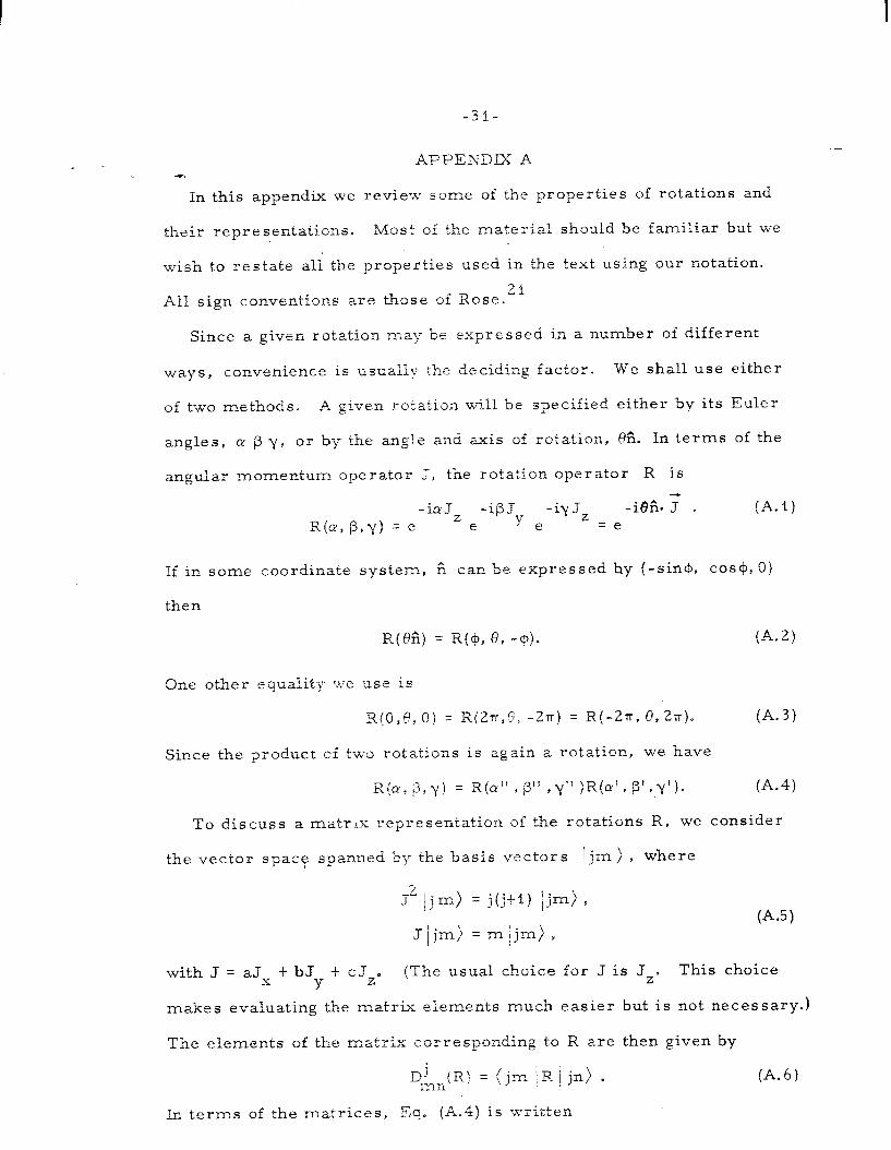
APPENDIX A -h

In this appendix we review some of the properties of rotations and

their representations. Most of the material should be familiar but we

wish to restate all the properties used in the text using our notation.

All sign conventions are those of Rose. 21

Since a given rotation may be expressed in a number of different

ways, convenience is usually the deciding factor. We shall use either

of two methods. A given rotation will be specified either by its Euler

angles, a /3 y, or by the ang?e and axis of rotation, 8% In terms of the

angular momentum operator J, t’ne rotation operator R is

-iaJ -iFJ -iy Jz -i$ii. 7 . (A.11 R(a, p,y) = e ’ e y e =e

If in some coordinate system, fi can be expressed hy (-sin+, cos+, 0)

then

R(%) = R(+, 8, -Q). (A.21

One other equality we use is

R(O,G,C!) = R(2n,8, -2-n) = R(-2rr, 8,2~r). (A.31

Since the product of two rotations is again a rotation, we have

a(~: g,y) = R(Q”, p” ,y’: )R(a’, P’,~‘)- (A.41

To discuss a matrix representation of the rotations R, we consider

the vector space sTanned by the basis vectors 1 jm) , where

JZ 1 jm) = j(j+1) ljm) p i . (A.5)

J\jm) = mijm) 9

with J = aJx t bJy -f cJzs (The usual choice for J is Jza This choice

makes evaluating the matr%x elements much easier but is not necessary.)

The elements of the matrix corresponding to R are then given by

Dads = (jm jR 1 jn) . (A.61

In terms of the matrices, Eq. (A.41 is written

-32-

&pressing R in terms of the Euler angles and making the usual

choice of J = Jz, the matrix elements simplify to

Dh(a., /3,y) = e -i(mcutny)dj

,,@I * (A. 8)

where the functions d’ ,,(F) are real. These functions satisfy the gen-

eral relations

dmn(P) = (-l)m-n dim@) = (-i)m-n dim-,(P),

dinW) = (-l)j-n dtmn(P) = (-l)jtm dmmn(@),

(A.9)

d’j&tZrr) = (-1)‘j dmn(P),

$!&-P) = +,(P) .

The normalization integrals are

We use the same conventions as the Particle Data Group for the

vector addition coefficients : 22

C(j,, j,, j Im1,m2) = (jij2mp2 Ijlj2jm) - (A-11)

We have the following relations for these coefficients:

C(j,, j,, j Im,,m2) = t-1) ji+j2-j

C(j,, j,, jlm2,ml)

(A. 12)

= (-1) ji+j2 -j

C(j,, j,, j l-ml9 -m2Js

-33-

APPENDIX B -h

We consider the case of a + b - c i d using our normalization of

states. From Eqs. (29) and (32) we ihave the differential cross section:

2 da q ‘- z ‘f I2 b4ipa+Pb-P,-nd)? E c 2

F /.L 1 i;’ & &, E

C d and

tB.1)

(B-2)

Assuming that both b and d are in x states, we have from Eq. (38):

fp = T fP4) -. 1/2

2 z: JLS

i (2Li”i) (ZL’tl)] i/‘2 qua, Ob, slp,, -pb)

L’S!

(B.3)

XCIL,S,J/O,~a-~b)Ci~c,ad,S!I~ C

, -pid)C(L’,S’, Ji0,~,-r”~)

x D,” / c-b-$.J ii,-pb” -‘beam) (8 =0, qJM, L’S’ITI 5 = 0, pJM, LS ) .

For simplicity we take the beam to be along the z-axis, in which case

+ PC --P-d Fa-%$

(c-l beam) = I+ Pc-Pd ‘a-%

(c-l). (B-4)

We now have

(B. 5)

where w represents the polar angles of c in the CMS. Using conser-

vation of energy and C.MS momentum together with F = PW, we have

do z(~~)-’ T I& i w-+w2~‘t~~l 1’2c(ua, Oh’ s/pa, -p,) L!S’

fB.6)

xC(L, S, JiO,~a-~b!iliac,od,S’t~ 9 -+,)C(L’,S’, JIO,~.L~-~~) C

XDJ F c-I-Ld pa-p”b

10 -I) t&O, qJM, L’S’IT&=O, pJM, LS)[’ d2 w.

Using Eq. (A.1$) and fAtegrating over d2w, using the normalization of

the vector addition coefficients, the cross section becomes

-34-

-lT 2Jtl r ~{~=O,qJM,L’S’~Tl~=O,pJM,LS)

G= pT f+ (2Gatl)(ZGbt1) cs L’S fB.7)

- Forahe case of nN * nN, L and L’ are determined by parity, S = S’,

and we have

(B. 8)

Thus we see that our equations reduce to the usual equations for the

two-body process.

APPENDIX C

This appendix, along with the following two appendices, details

derivations of text equations. Here we derive Eq. (64). The total

cross section is given by

T,(W, wj)Tm (W, wj) s dw2 i j

dcosej dco&d$.

J J

From Eq. (45)s with our choice of axes, we have

2 gPgP:: = w

nm r3pQ q

[ (2L+l)(2L’;1)~2Lj’l)(ZL;flj!Zljfl)rZ

j k

1;+1j] i/2

x qu, sf , 7 10, p.,-pb)

“\IZx, c(Gj,jj jsj !cLj, I . ’ j

-Xj) C( Lj, Sj, J jO,‘Lj‘“j) c( Gj >j’., S’. 1 J

1-L 3

-Xi'

X C(L;,S;, J’ /O,p FY

x DJ p.-A. pa-pbbj'Pj'Yj) Di’-*Ai I J j j pa-pb

(rrj~ Pj~Yj)

x,Fv c(G ,G ,S.lV - k 1

k 1 J k v,)C(lj,sj,.jjiO, vk-yl)C,(nl~Vrrip’iIv:, -vi! P

Vk Vi . X C(l;, s;, ‘;I O,vi,-vi)

’ j ’ d-)i

iC.la

(C.lbj

(CIC)

(C. Id)

(C. le)

(C. If)

-35-

- Xd

“k fe!) d 5

(-e!)d Ol 5- vl 01-“i

“ki”k J vp1 .I vi+

t-11 -

To evaluate the total cross section, we will discuss each of the parts

separately. Using Eqs. (A.7) and (A.9) and summing over pk and ~1,

line (C.lg) becomes

‘k (ok, d f-$/l dvk’-4, j ’ Ok

(Ok) d 5 *1 ‘lVk ‘ivi

‘ki”k ! Vl (4;)d (-ei ) (-1)

‘iI*1 J t-11

=d ‘k

(Old 4

t(O) (-1) ol-vl

t-11 Gl-“i

‘kV;c Yl (C-2)

= 5 vv’ 6

‘K k vv’ *

1 1

In (C.id) we have

DJ

‘lj -‘j ~a-~b

~2 DJ cc. 3) MM’ Yj ”

(j-liD~:~h, J j

M, (j-l) D& ~ ~ ($,o, -$I a-b

J / ::: x DIM pa--s @B, -gg.

Using the normalization Eq. (-4.11) and integrating over d cos @d$

gives

i (C.ld) d cos @ d$ = E DJ ,+ ,(j-‘) D

J’ $ MM’ ~j j

-Xl Ml (j-1)2+JJlbMM’

5 j

= DJ pj - xj (C-4)

-36-

With the delta functions from Eqs. (C.2) and (C.4), the integration

of line fC.lf) over d cos 8. yields 3 4

i

ijj j;

5 ‘k-+~

(‘j) d_, lj Vk-V1 (‘jJd ‘OS ‘j = & 'j.ji.'

J J J ic. 5)

With this we see that isobars with different total spin, jj, do not inter-

fere in the. total cross section.

With the delta functions and the orthogonality of the vector addition

coefficients, line (C.le) reduces to

x ‘k’l

c(c k 1 3

#o , s. 1 vkp -vl)c(lj, sj9 jj / 0, Vk-vl)C(ak’Ol’ “) j ‘/k’ -v1) a

(C. 6)

Similiar ly

z (C.ib) = * 6LL, $S’ 9 ‘a%

(6.7)

With these intermediate results the total cross-section is given by

x 6 JJ’ ‘LL’ 6LjL1j oSS~6S.S!61.1!6s.si.

JJ JJ JJ

x -- 4n 2

2J+1 2jj+1 TJW, w. J)Tm(W, wj)dw;

2J-FJ (20-a+i)

T,(W, wj j i 2 dwf s

(C. 81

-37-

APPENDIX D

Here we derive Eq. (70) of the text. From Eqs. (45) and (48) we have

g-IL=w n IT i

[ (2L+l)(2Lj+l)(21jt’)1

XC(ua, Ub’ s t -Pa’ P-b ) C(L, S, Ji 0, -pa++,) (D-la)

j C(Lj, Sj9 JI 0, -pj-Xj)DJ -‘“j-‘j

-tL +EL a b

(D.lb)

‘j x vxv G(akf~l~ sj 1 vk~ -vl) c(lj’ sj, jj 1’9 Vk-V1) d-l v k 1 j keV1

(ej)

(D. Ic)

Xd ‘k

(04;) d “1 9-Y

. ‘k-s ’ vl-pl

(-0:) (-1) (D. Id)

Using Eq. (A. 9), 1 Fne (D.ld) becomes

dak ( &, dul (-Of) (-I) o1-vl

= (-1) ‘ktpk f-1)

Vl+tJ.l $K

y-i*;, J vpl - vapk(e;)

Xd “1

(4;) (-1) =1-“1

-“gJ? (D-2)

= (-1) (-1 jvktb duk (e”) d 9

-‘kpk 1 (-et ),

-vlP1 3

and line (D. Ic) becomes

d!lj\ v (621 = (-1) xJ-vksy 3

j keV1 ’ dA. - (6.).

J ‘k+‘l 3

Since

(D.3)

(D-4)

-38-

line (D-lb) reduces to

0.5)

Using Eq., (A.lO) and making all t%e substitutions,

[ 1 b4

-P‘= gn

w wi 71 1TPQjqk

~3 .tj.-S.

(--I)

Lj*sj-J(m~~ J J Jctg j I j’ j’

sj ‘pj,tAj)

- I c(Lj,sj, J %pj+Aj)

x(-1)2J(-i) J ~.’ ‘j+‘-La-~ DJ*

i*j+h, ‘“a-14, (crj~ Pj'Yjj

J

XZ ‘kVl

.t jj j 0, - J

VLf vj 1 K

-A.-v tv x (-1)

J k l,jj A. - w

I ‘kSvl J

X(-f) CT 1%

(-1)

Since X., V 3 k’

and v1 are just dummy variables, we can make the change

A .-t-Xj9 vk + - vk, and v1 + - vl. Thus 3

L+L.-l-1. g-p= (-1) J J (-1)

0 a+Pa (-1)

“b--s (-1)

‘J k+Pk (-1)

*k”l go t n n *

(D. 7)

-39-

Since we have assumed that L, L., and 1. are chosen to conserve - J J

parity, we have that

LSL.fl.- LSL .+1. 1 = 17, ~b “j rlk rll (-1) J J = T(--j) J J (D. 8)

where q is the product of all five parities. Finally then

(D. 9)

APPENDIX E

In this appendix we derive Eqs. (74) - (76) for the interchange of

particles k and 1. From Eq. (73) we have the following changes under

inter change:

w+w 2 2 2 22 2

wj - w.,

J Wk- WI’ w1 --* Wk’

pa - ii,, &,+ pb’

5 - ~j,“k-“~“il~ ‘4c’

Most of the changes are obvious. For convenience we shall let

P’ = (~a~b~j~l~k~ ’ We also indicate the type of isobar with an

additional subscription on g.

For j-type isobars, we have

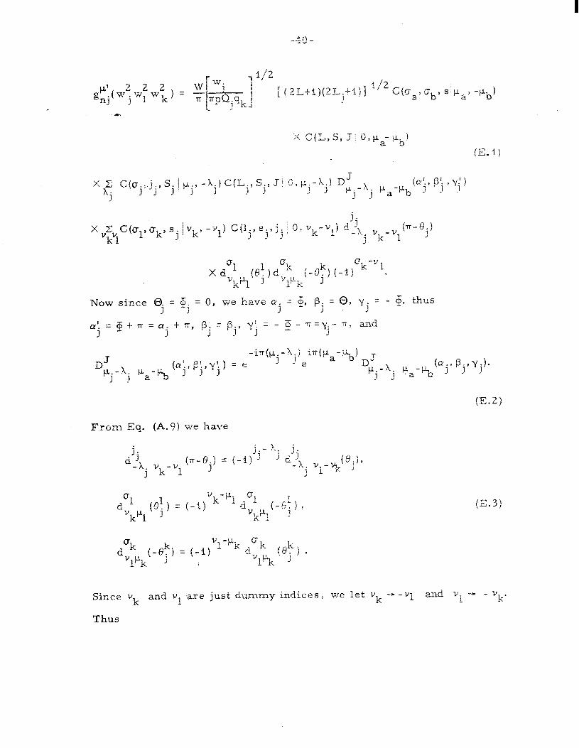
“k-VI (2) 6-i) .

Now since ej = $j = 0, we have CI~ = $, /3: = 8, yj = - $, thus J

I - 7

- ij t TT = a. t r9 “i = pi, y; = - 4 - r=y:- 7, and 3 J i

v -y j k ?

(7T-6j) = (-i)

(6P) = (-1) ‘k% ’

(E.3)

Since Vk and v1 ‘are just dummy indices 2 we let vk - -vi and v 1

+ - v k’

Thus

-4l-

x c (Da, Cb , s 1 pa, -+J C(L,.S, J 1 0, pa-pb)

' ~ '(Cj'jj"j 1 ~j' -1 ) C(Lj,Sj, J 10, pj-lj) (-1) '"a-tk-~j'Xj

j 1

1.-l-S.-j. 1) J ’ J (-1)

jj-Xj x ~

‘kV1 c(c ,a , s ’ Vk’ -vl) c(‘j, sj,lj 1 O, ‘k-‘l) (-

k 1 j!

(E.4)

-‘j x d-X v j kBVl

(ej)

Xd Ok (ek) d al

‘k’k J vl% (-1)

‘k-vk t-11

‘k+l

= ($4 (-1) s . tcktol 1 (-1)

~,-)lb-lij-i*k-~l ~ 22 2 gnj(Wj Wkwl ). (74)

For k or l-type isobars, the inter change is only meaningful when

k and 1 are the same type of Particle. In this case similar calculations

give for k-type isobars:

,;;tw; wpw;, = (-1) ‘k (-

and for l-type isobars

(75)

I1 t-11

‘lSQjfgk (_ 1) Fa-Pb-P‘j-~-'l gp nk (wf w; w2,,’

(76)

Footnotes and References

t Present address: Lawrence Livermore Laboratory, P. 0. Box 808, Livermore, California 94550.

t Present address: DESY, 2006 Hamburg 52, Germany.

9 Present address: Laboratory for Nuclear Physics, Oxford TJniversity, Oxford, England.

1.

2.

3.

4.

5.

4.

7.

8.

9.

10.

11.

12.

13.

14.

15.

S. 3. Lindenbaum and R. J. Sternheimer, Phys. Rev. 22, 1874

(1957); 106, 1107 (1957); 109,1723 (1958); a23, 333 (1961).

M. G. Olsson and G, V. Yodh, Phys. Rev. 145, 1309 (1966).

B. Deler and 6. Valiadas, Nuovo Cimento e, 5.59 (1966).

J. M. Namyslowski, M. S. K. Razmi, and R. G. Roberts,

Phys. Rev. -157, $328 (1967) s

D. Morgan, Phys. Rev. 166, 1731. (1968).

M. DeBeer et al,, Nut!. Phys. B12, 617 (1969).

M. G. Bowler and R, J. Cashmore, Nucl. Phys. B-17, 33-1

(1970).

A. Baracca and S. Bergia, IXFN/AE - 69/3 (1969 ).

D. H. Saxon, J. H. Mulvey, and W. Chinowsky, Phys. Rev.

D_Z, 1790 (1970).

6. C. Wick, Ann. Phys. (N-Y.) 18, 65 (1962).

J. D. Jackson, Nuovo Cimentoz, 1644 (1964).

A. 3. Macfarlane, Rev. Mod. Phys o 34, 41 (1962). --

D. J. Herndon et ai., Lawrence Berkeley Laboratory Report

LBL-1065 (1973) to be published.

M. Jacob and G. C. Wick, Ann. Phys. (N. Y. ) 1, 404 (195?!.

S. Berman and M. Jacob, Phys. Rev. 139, B1023 (i965).

-43-

- 16. H. P. Stapp, Phys. Rev. 103, 425 (1956).

17. The factors (pl4Wj l/2 and (Qi/4 Wj d/2 come from our choice

of normalization. The factors p L and QF need to be changed;

see F. von Hippel and C. Quigg, Phys. Rev. D 2, 624 (1972).

18. 6. Smadja, Lawrence Berkeley Laboratory Report LBL-382

(19711, unpublished.

19. A similar discussion occurs in R. 3. Cashmore and A. J. G.

Hey, Phys. Rev. D 6, 1303 (1972). -

20. G. Ascoli et al., Phys. Rev. D z, 669 (1973).

21. M. E. Rose, Elementary Theory of Angular Momentum

(Wiley, New York, 1957).

22. Particle Data Group, Rev. Mod. Phys. 45 S1 (1973). 2

-‘IO = 5 / fA++i2 + [A+-12 + !A +I2 + IA -- i2j

IoAx = Re [A++ A+* ei"] + Re [A-+ A-"_ eial

[A-+ A,* e ia

1 IA 0 Y.

= Im [A 'A * P] + fm -l-i- +-

I*+,_ I2 - jA--12j

(6) IOPX

= Rc [A,+ *_:I + Re [A+- A *I --

0-d IOPY

= -1m [A,+ A-+"] - Im [A+- A *] --

IOPP) = 4 r' !*+I2 + IA+-i2 - lA-+i2 - /A me 1'1

IODXX = Rc [A+- A-: e -ia] + Re [A++ A* ei"] --

IoDxy = -1m [A+- A-: esia] - Im [A++ A * eia] --

IODXZ = Re [A* A+* e ia] - Re [A-+ A * eiaj . --

-44-

Table I. Expressions for all observable quantities in the reaction MB- BMM. Amplitudes A pfpi = t- . I-l.f'i

with pfpi = f i/2 are written as

ID 0 YX

= -1m [A+- A-: eeia] + Im [A+ A * eia] --

ID 0 YY

= Re [A+ A-r eia] - Re [A ~- A-: emia]

IODJfZ = Im [A,+ A+* eia] -1m [A-+ A * eia] --

I ODzX = Re [&4+ A-:] - Re [A+- A + ] --

IoDzy = -1m [A++ A-:] + Im [A+- A *I --

l ’ IODzZ = =2- I I*++ t2 + I*-- I2 - b+i2 - i*+-12 ;

-45-

-h Figure Captions

Fig. 1. Notation for the reaction a t b + j + k t 1.

a) Quantities in the center of mass rest-frame.

b) Quantities in the diparticle rest-frame.

Fig. 2. Definition of angles in our coordinate system.

a) Beam angles in center of mass rest-frame.

b) Angles of particles j, k,l in center of mass rest-frame.

c) Angles of particles k,l in the diparticle rest-frame.

Fig. 3. Symbolic diagram of the effect of the Lorentz transformation

L on the momentum vectors. Although the diagram is not

quantitative, it does show the correct direction for the various

angle s.

Fig. 4. Illustration of the effect of the rotation R(-+, 0, +) on the

axes OXYZ.

Fig. 5. Final state helicity frame axes for particle j.

(b) Fig. 1. XBL736- 3236

-47-

Qj

Y

P a

Qj

Fig. 2. XBL736-3237

I

-48-

X81-736 -3238 Fig. 3.

X X

Z

----

-se-

x N

2

: .

‘N

-5o-

z

Z I

XBL736-3240 Fig. 5.