subsidies to public firms and competition modes under a ... · subsidies to public firms and...

DPRIETI Discussion Paper Series 18-E-001

Subsidies to Public Firms and Competition Modes under a Mixed Duopoly

HIGASHIDA KeisakuKwansei Gakuin University

The Research Institute of Economy, Trade and Industryhttp://www.rieti.go.jp/en/

http://www.rieti.go.jp/en/index.html

1

RIETI Discussion Paper Series 18-E-001 January 2018

Subsidies to Public Firms and Competition Modes under a Mixed Duopoly1

HIGASHIDA Keisaku

School of Economics, Kwansei Gakuin University

Abstract This study experimentally examines whether subsidies to a state-owned enterprises (SOE) change the behavior of a private firm or the SOE under a mixed duopoly. Following Hampton and Sherstyuk (2012), we conducted a series of laboratory experiments adopting a two-stage capacity-price decision-making duopoly setting. We adopted two treatments in terms of types of subsidies: one is a subsidy for production/sales and the other is a subsidy for capacity building. The results indicate that even a small amount of subsidy can influence the choices of capacities and prices of both types of firms. Production subsidies increase capacities of both private firms and SOEs, and, accordingly, the prices of both types of firms decrease, while capacity subsidies decrease capacities of private firms. Because the competition for capacity building between two firms becomes less severe, the profits of both firms increase and, interestingly, the idle capacities of private firms decrease. Moreover, both social and domestic surpluses increase in the case of production subsidies, but decrease in the case of capacity subsidy. In the former case, severe competition mitigates the distortion caused by imperfect competition. We also find that the firm attributes and behavior in the past significantly influence capacity choices.

Keywords: Laboratory experiments, Mixed duopoly, State-owned enterprises, Competition modes. JEL classification: H25, H44, L13, L32.

1 This study is conducted as a part of the Comprehensive Research on the Current International Trade/Investment System (pt.III) project undertaken at the Research Institute of Economy, Trade and Industry (RIETI). The author is grateful to Kenta Tanaka (Musashi Univ.) for assistance in operating Z-tree programs. The author is also grateful for helpful comments and suggestions by Eiichi Tomiura (Hitotsubashi Univ.), Tsuyoshi Kawase (Sophia Univ.), Satoru Kumagai (Institute of Developing Economies, JETRO), Mai Fujita (Institute of Developing Economies, JETRO), Mariko Watanabe (Gakushuin Univ.), and Discussion Paper seminar participants at RIETI. The author also acknowledges the financial support from the JSPS under Grant-in-Aid for Scientific Research (B, 15H03347).

RIETI Discussion Papers Series aims at widely disseminating research results in the form of professional

papers, thereby stimulating lively discussion. The views expressed in the papers are solely those of the

author(s), and neither represent those of the organization to which the author(s) belong(s) nor the Research

Institute of Economy, Trade and Industry.

2

1. Introduction

The positive and negative effects of the entry of state-owned enterprises (SOEs) into markets

have been discussed for the past several decades, both in the academic field and political

arena.2 Because the objective of SOEs is theoretically the weighted sum of profits and social

surplus, entry of an SOE into a market increases social surplus when the market is imperfectly

competitive. The entry lowers prices and increases consumption and, accordingly, consumer

surplus. The market structure that contains both private firms and SOEs is called a mixed

oligopoly. 3 Many articles have theoretically examined mixed oligopoly in the past few

decades (Matsumura, 1998; Matsumura, 2003; Matsumura and Matsushima, 2004; Lu and

Poddar, 2006; Ishibashi and Kaneko, 2008; Ohnishi, 2009; Kitahara and Matsumura, 2013;

Luo, 2013, among others). Several articles have also investigated regulations and subsidies

relating to mixed oligopoly (for example, Matsumura, 2012; Scrimitore, 2014).

However, when we consider subsidies to SOEs, the problem is not only a domestic one

but also an international issue in the real world. Consider an example in which both domestic

SOEs and foreign private firms are engaged in a product market. If the government provides

subsidies to the domestic SOEs, the situation becomes unfavorable for foreign private firms.

In general, a production subsidy acts like a decrease in marginal production cost, making a

subsidized SOE more competitive against private firms. This may drive out foreign private

firms from the domestic market. Even when they compete with each other in an international

market, subsidies gives SOEs a stronger incentive to increase their outputs, which leads to a

decrease in the price of the product, not because of any innovation by the SOEs, but because

of the subsidies. Thus, private firms lose their profits. Moreover, in contrast to subsidies to

2 Public firm is usually used for this type of firm in the field of economics. However, considering the purpose of this paper and the ongoing RIETI project, we use state-owned firm (SOE) in this paper. 3 When one private firm and one SOE enter a market, the market structure is referred to as mixed duopoly.

private firms, subsidies to SOEs are likely to be easily excessive because of political reasons;

SOEs usually have networks and connections with authorities that manage subsidies.

Moreover, the objectives of managers in SOEs are often neither profit maximization nor

welfare maximization. Rather, they may act to obtain power in their institutions or political

power. The World Trade Organization has been discussing subsidies for SOEs for the past

decade in its negotiations.4 Similar to other subsidies, this type of subsidy is strictly restricted

for partner countries to use.

As noted above, mixed oligopoly has been theoretically analyzed in detail in the field of

economics. However, there is little experimental evidence for this market structure. Although

Du et al. (2013) carried out an experiment under the structure of mixed duopoly and observed

the behavior of a public firm, they focused on a delegation problem. The merit of using

experimental methods to analyze the effect of subsidies for SOEs under mixed oligopoly is

that changes in the competition structure can be observed and clarified. Theoretical studies

focus on issues relating to the characteristics of markets and firms, such as quality, product

differentiation, uncertainty, and partial privatization given the competition mode. However,

government subsidies to SOEs can change the competition structures between private firms

and SOEs. An experimental approach is able to elucidate these changes caused by policy

changes.

The purpose of this paper is to clarify the effect of SOE subsidies on capacities, prices, and

profits of both a private firm and an SOE under the setting of mixed duopoly. We also examine

if this type of subsidy is harmful by investigating the effect on social surplus. To this end, we

adopt a two-stage capacity-price decision-making setting. In this setting, subjects choose their

capacities simultaneously in the first stage and, then, choose their prices

4 Several articles examined international mixed oligopoly and international trade issues (Chang, 2007; Ohnishi, 2008; Lee et al., 2013; Ou et al, 2016).

3

4

simultaneously in the second stage, during which we consider the factors of both quantity and

price competition. Kreps and Scheinkman (1983) set up the theoretical model and proved that

the equilibrium outputs are the same as those in Cournot equilibrium. 5 The two-stage decision-

making structure has been used for experimental studies under oligopoly (Davis, 1999; Muren,

2000; Goodwin and Mestelman, 2010; Hampton and Sherstyuk, 2012). In contrast to the

theory of mixed oligopoly, all of the firms’ capacities are not necessarily used for production

in the second stage. Idle capacities may exist when subjects hold capacities excessively in the

first stage and when they give up using part of their capacities for production to avoid a sharp

drop in the price.

This paper has three features. First, we examine two types of subsidies for SOEs: a

production/sales subsidy and a capacity subsidy. The former subsidy is provided according to

the sales/production amount, which implies that this subsidy directly influences the decision-

making of SOEs in the second stage. In comparison, the latter is provided according to the

amount of capacity holding, which implies that this subsidy directly influences the decision-

making of SOEs in the first stage. Even if capacities are not used for production (idle), the

SOEs receive subsidies.

Second, we carry out several treatments for a production subsidy, with different amounts

of per unit production subsidy across treatments. We introduce these treatments because the

amounts of subsidy may also influence the degree of responses by SOEs and, accordingly, by

private firms.

Third, we consider not only social surplus but also domestic surplus. Social surplus, which

is defined as the sum of consumer surplus and profits of both the private firm and the SOE, is

equivalent to world welfare in the context of international trade theory if the private firm is a

5 Durham et al. (2004) examined the oligopolistic competition in the presence of fixed cost for capacity holding.

5

foreign firm and the SOE is a home/domestic firm. On the other hand, if the objective of the

domestic government is to maximize domestic surplus, the profits of the foreign private firm

are excluded from the objective function. Hence, we also consider domestic surplus, which is

defined as the sum of consumer surplus and the profits of the SOE.

The main results are as follows. First, even a small amount of subsidy can influence the

choices of capacities and prices of both types of firms. Second, a production subsidy increases

the capacities of both private firms and SOEs and, accordingly, the prices of both types of

firms’ products decrease. These changes indicate that quantity competition becomes more

severe after a subsidy is provided. Third, on the other hand, a capacity subsidy decreases the

capacities of private firms while the capacities of SOEs increase. Because the former effect

dominates the latter effect, total capacities also decrease. With a capacity subsidy, the quantity

competition between both types of firms is less severe, the profits of both types of firms

increase and, interestingly, the idle capacities of private firms decrease. Fourth, both social

and domestic surpluses increase in the case of a production subsidy but decrease in the case of

a capacity subsidy. In the former case, the severe competition mitigates the distortion caused by

imperfect competition. Fifth, the firm attributes and behavior in the past significantly influence

capacity choices and price setting. Whether a firm is a private one or an SOE significantly

influences capacity choices; in some cases, capacity choices and price setting are influenced by

the behavior of the partner in the previous round.

The structure of the rest of the paper is as follows. Section 2 describes the design of the

experiment sessions. Section 3 reports the results of the experiment. Section 4 discuss policy

implication, and Section 5 provides concluding remarks.

2. Design of the Experiment

2.1 Design and Demand Structure

6

We follow the basic design used in Hampton and Sherstyuk (2012), which is a type of two-

stage capacity-price-choice duopoly model. Two subjects are randomly paired in each session,

and they stay in the same market throughout the session they participate in. Both subjects act

as sellers in the market under specified demand conditions that are certainly known to them.

Basically, each round consists of two stages. First, both subjects make simultaneous capacity

choices. When both/all the subjects determine their capacities, each subject is informed about

the capacity chosen by the other and the total capacity of the market that s/he enters. Second,

each subject chooses a price simultaneously. As explained in the next subsection, one of the

two subjects plays the role of a private firm, while the other plays the role of an SOE in the

quantity-price-setting game.

Each seller faces a constant marginal cost for holding capacity, which is 20 experimental

dollars per unit.6 As our purpose is to observe individual behavior and market situations with

production/capacity subsidies, we exclude the fixed cost because it makes the structure of the

experiment complicated and confusing. However, subjects must pay marginal costs according

to the capacity they possess rather than the amounts of goods produced. Even if the production

amount is smaller than the capacity, the cost is equal to 20 experimental dollars times the

capacity. Thus, this marginal cost for holding additional capacity may act as a fixed cost in the

sense that the cost is sunk when they choose their prices.

Throughout the experiment, the subjects face a demand condition given by the following

formula:

Q = 200 - 2p (1) where Q and p denote the total supply by the two entrants and the market price, respectively.

Each experiment session consists of two phases, the details of which are explained in the next

subsection. The first phase, which is referred to as Phase 1, consists of ten rounds, while the

6 We use the term “experimental dollars” for the money used in the experiment sessions.

7

second phase, which is referred to as Phase 2, consists of eight or seven rounds.

In the experiment, the table of quantities and prices that reflects demand condition (1) is

distributed at the beginning of the experiment (See Figure 1).

2.2 Treatments

As noted above, one person in each pair plays the role of a private firm, while the other plays

the role of an SOE. The objective of the former player is the maximization of his/her own

profits throughout the experiment. Each subject who plays the role of a private firm recognizes

that her/his acquired points/rewards in the experiment (acquired experimental dollars) are

defined as follows:

Acquiγed expeγimeηtαl dollαγs foγ α pγivαte fiγm = Pγofits In the following, we also use rewards to refer to acquired experimental dollars, which may be

different from profits.

We conducted two main treatments and three additional treatments in terms of the

objectives of the latter player (SOE). In Phase 1, the objective of an SOE is common for the

two main treatments, which is defined as follows:

Acquiγed expeγimeηtαl dollαγs foγ αη SOE = 0.7 × Pγofits + Sαles This objective implies that the marginal cost of capacity holding is decreased by approximately

1.43, as long as the capacity is used for production. In other words, capacity holding is not

directly subsidized. SOEs have stronger incentives to produce than private firms do. Unless

the total production amount is greater than 160, the behavior of the private firm increases social

surplus.

The objectives of an SOE in Phase 2 are different between the treatments. In the first main

treatment (SS3), the objective of an SOE is defined as follows:

Acquiγed expeγimeηtαl dollαγs foγ α SOE = 0.7 × Pγofits + 4 × Sαles.

8

Each SOE has a stronger incentive to increase its production/sales in Phase 2 than in Phase 1.

This change implies that the production/sales subsidy provided to the SOE increases. In the

following analysis, we refer to this type of subsidy as a production subsidy.

In the second main treatment (CS3), the objective of an SOE in Phase 2 is defined as

follows:

Acquiγed expeγimeηtαl dollαγs foγ αη SOE

= 0.7 × Pγofits + Sαles + 3 × Cαpαcities In contrast to treatment SS3, each SOE has a stronger incentive to increase its capacities in

Phase 2 than in Phase 1. This change also considers that the capacity subsidy provided to the

SOE increases. Note that capacity holding is subsidized even if the capacity is idle.

To verify the effect of an increased amount of production subsidy and the effect of a new

starting level of production subsidy, we conducted three additional treatments, which are

referred to as SS1, SS5, and SS9. Similar to the main treatments, the objective of a private

firm is the maximization of its own profits in both phases.

The objective of an SOE in Phase 1 of SS1 and SS5 are the same as that of SS3. On the

other hand, the objectives of an SOE in Phase 2 of SS1 and SS5 are defined as follows:

Acquiγed expeγimeηtαl dollαγs foγ α SOE = 0.7 × Pγofits + 2 × Sαles,

and

Acquiγed expeγimeηtαl dollαγs foγ α SOE = 0.7 × Pγofits + 6 × Sαles,

respectively. The effect of an increase in the production subsidy in treatment SS1 are expected

to be smaller than that in treatment SS3, while the effect of an increase in the production

subsidy in SS5 are expected to be larger than that in SS3.

Finally, the starting level of an incentive of an SOE to increase its production/sales in SS9

is different from that in the other treatments. The objective of an SOE in Phase 1 is defined as

follows:

9

Acquiγed expeγimeηtαl dollαγs foγ α SOE = 0.7 × Pγofits + 6 × Sαles. On the other hand, the increase in the production subsidy in SS9 is the same as that in SS3.

Thus, the objective of an SOE in Phase 2 is defined as follows:

Acquiγed expeγimeηtαl dollαγs foγ α SOE = 0.7 × Pγofits + 9 × Sαles. 2.3 Sessions and Procedures

We conducted three SS3 and three CS3 treatments. Moreover, we conducted one SS1, one SS5,

and two SS9 treatments. In each session, the number of participants were eight, ten, or twelve,

which implies that the number of markets in each session was four, five, or six. The participants

were undergraduate students of Kwansei Gakuin University. See Table 1 for the details of the

sessions. We did not exclude students of any specific departments. Thus, our sample includes

students who specialize in various fields, including business, economics, law, literature, and

social studies. Each student participated in only one session, and those students were paid an

average of ¥3533.467 based on their results.7 In the beginning of each session, the subjects

answered a questionnaire intended to measure their risk preference and, then, they were directed

to read the instructions for about 10 minutes. 8 Then, for a more precise understanding of the

instructions, an instructor read them out loud.

In each round, the subjects were given 30 seconds to determine their capacities in Stage 1.

When all the subjects determined their capacities, they proceeded to Stage 2. At this stage, the

subjects were given 70 seconds to determine their prices. They were allowed to use the

7 Before the subjects began the capacity-price-setting game, they were told that 6 experimental dollars would be converted into ¥1 for real payments. However, before we began the series of the experiment sessions, we expected that the acquired experimental dollars would be greater than those the subjects actually acquired. Thus, in the first two sessions, both of which are SS9 treatments, subjects are told that 12 and 8 experimental dollars would be converted into ¥1 for real payments. However, in the end of those sessions, the subjects were told that the conversion rate was changed to “6 experimental dollars = ¥1.” 8 See Figure 2 for this questionnaire.

10

calculator function on their computer screens. When a subject determined the price, s/he

entered the price and clicked the “OK” button. When all subjects determined their prices, they

proceeded to the recording stage, in which they wrote down the results. They saw sales

amounts, prices, and profits of both participants and their own acquired experimental dollars

on the screen. This recording stage continued for 20 seconds.

In this paper, we use technical terms specific to industry and cartels to describe the

experiment design and the results. However, in the experiment, the subjects were shown more

neutral terminologies. Moreover, in the following sections, we refer to the human participants

who play the roles of private firms in the experiment as "private firms" and the participants

who play the roles of SOEs as "SOEs” for brevity. We conducted the experiment using the

University of Zurich’s A-tree program (Fischbacher, 1999).

3. Results

3.1 Market Variables First, we look at the aggregate data, averages, and standard deviations to get an overview of

the outcomes of the experiment. For our mixed duopoly experiment, there are two benchmark

pairs of capacities and prices.

The first benchmark is a Cournot equilibrium with two private firms. Suppose that both

firms are private firms and choose capacities and quantities in each stage to maximize their

own profits. According to Kreps and Scheinkman (1983), the equilibrium capacities and,

accordingly, the prices are theoretically the same as those of a Cournot equilibrium. That is,

each firm’s capacity/sales, total capacity/sales, and prices are 160/3, 320/3, and 140/3,

respectively. The second benchmark is a Bertrand equilibrium with two private firms. Because

the marginal cost of capacity/production is 20, the total capacity/sales and price in equilibrium

are 160 and 20, respectively. Figures 3 and 4 show the trend of average market capacities,

11

prices, and sales of SS3 and CS3 (the two main treatments), respectively. According to these

figures, the market values seem to be between those of Cournot and Bertrand equilibria with

two private firms in Phase 1. These trends are similar to the results of Hampton and Sherstyuk

(2012). In Phase 2, the capacities are greater than those of a Bertrand equilibrium with two

private firms; this is possible because SOEs have stronger incentives to increase their

capacities and sales.

Because our focus is the effects of increases in subsidies on capacities, prices, sales, and

profits, we investigate the effects on market variables by using the Wilcoxon Signed-Rank

Test. The results, which are P-values, are shown in Table 2 for SS3 (Sessions 4, 5, and 8) and

CS3 (Sessions 6, 7, and 9). As long as we focus on market variables, there seems to be no

common differences between the values of Phases 1 and 2 across sessions. For example, when

we focus on SS3, all variables of both phases in Session 4 are significantly different from each

other, while there are no significant differences in each variable between both phases in

Sessions 5 and 8. On the other hand, when we focus on CS3, there is a significant difference

in profits between both phases in Session 6, while there are no clear differences in profits in

Sessions 7 and 9.

3.2 Variables for Private Firms and SOEs

The result that indicates that increases in production/capacity subsidies may not influence

market variables does not necessarily mean that there is no effect on the behavior of either

private firms or SOEs. They may change their decision-making according to policy changes.

Thus, in this subsection, we investigate capacities, prices, sales, idle capacities, and profits for

both private firms and SOEs separately.

First, we examine private firms. The results are shown in Table 3a. Overall, when focusing

on capacities and prices, those values are between the Cournot and Bertrand equilibria in a

12

two-private-firm-duopoly case. However, when focusing on sales, it seems to be almost

equivalent to the sales in the Cournot equilibrium.

Focusing on the changes in the averages between two phases, a clear contrast between two

policies is observed. In the case of a production subsidy, capacities, sales, and idle capacities

increase while prices and profits decrease. These facts imply that competition becomes more

severe with an increase in a production subsidy. Private firms expect that rival SOEs will

increase their sales more aggressively, and they respond to this policy change by lowering

their prices. An interesting point is that this change in the second (price setting) stage makes

private firms increase their capacities in the first stage. Private firms may use capacity building

as a threat. On the other hand, interestingly, the capacities and sales of private firms decrease

and prices and profits increase with an increase in capacity subsidy. Idle capacities also

decrease. It is likely that private firms expect that rival SOEs increase their capacities

aggressively because this type of subsidy directly encourages capacity building of SOEs, and,

accordingly, the private firms decrease their capacities in response to this change in the

situation. We investigate the situation more precisely using the Wilcoxon Signed-Rank Test.

The analysis, shown in Table 3b, reveals the following results.

Result 1. In response to an increase in a production subsidy, private firms lower their prices.

Their profits decrease on average. On the other hand, in response to an increase in capacity

subsidy, private firms decrease capacities. Idle capacities decrease as a result, on average.

The Wilcoxon Signed-Rank Test results indicate that a change in subsidy that directly

influences the first stage variable changes the decision making in the first stage, while a change

in subsidy that directly influences the second stage mainly changes the decision making in the

second stage.

13

Second, we examine SOEs. The results are shown in Table 4a. Overall, when focusing on

sales and prices, it is obvious that those values are between the Cournot and Bertrand equilibria

in a two-private-firm-duopoly case. However, when focusing on capacities, except for Phase

1 in the case of a production subsidy, the amounts are greater than those in the half of sales in

the Bertrand equilibrium.

The changes, on average, between two phases are different from those for private firms. In

the case of a production subsidy, the changes in capacity, price, sales, and profits are similar to

those for private firms. However, idle capacities decrease. Considering that subsidized SOEs

are incentivized to increase their sales, this result is intuitive. SOEs have incentives to increase

their sales given their capacities in the second stage. In the case of capacity subsidy, in contrast

to the changes in variables for private firms, SOEs increase capacities and sales, although the

increased amounts are smaller than with a production subsidy. Because private firms decrease

their capacities and sales, the average price in Phase 2 is higher than that in Phase 1. It is

verified that the effects of both types of subsidies on competition structure in the first stage are

different from each other. In particular, the Wilcoxon Signed-Rank Test analysis (P-values),

shown in Table 4b, reveals the following results.

Result 2. In response to an increase in a production subsidy, SOEs increase their capacities

and sales, and lower their prices. On the other hand, in response to an increase in capacity

subsidy, SOEs increase their capacities, while prices do not change, on average.

Now, let us examine total quantities and compare private firms and SOEs. First, as noted

above, the average capacities of SOEs are greater than the half of the Bertrand equilibrium

with a two-private-firm-duopoly case. However, total capacities of both private firms and

SOEs do not exceed the total supply in the Bertrand equilibrium, on average. Second, the

14

average prices for both private firms and SOEs increase in the case of a capacity subsidy. This

result implies that consumer surplus decreases due to an increase in capacity subsidy. Third,

although the directions of the changes in variables in the case of a production subsidy are the

same for both private firms and SOEs, the increased/decreased amounts are greater for SOEs

than for private firms. Considering that SOEs are subsidized, this difference is intuitive. Fourth,

the average profits of SOEs increase due to an increase in capacity subsidy. Because the

objective of SOEs is different from profit maximization, this result is interesting. SOEs have

an incentive to increase their capacities and, accordingly, the increased amount of average

profits is smaller than that of private firms. However, as described above, private firms decrease

their capacities by larger amounts on average, which prevents the market price from declining.

Consequently, even though SOEs increase their capacities and sales in response to an increase

in capacity subsidy, their profits increase.

3.3 Surpluses

Now, let us investigate the effects of subsidy on social and domestic surpluses. Social surplus

is defined as the sum of consumer surplus and the profits of both a private firm and an SOE.

Because subsidy is a kind of income redistribution, we do not describe it explicitly. On the

other hand, domestic surplus is defined as the sum of consumer surplus and the profits of an

SOE.9 In the real situation, subsidies to domestic SOEs were/are often international issues. In

such cases, the point is that the condition for competition is unfavorable to foreign private

firms. Moreover, it is sometimes argued that subsidized SOEs influence the international

market, which decreases the profits of private firms. Thus, it is natural to consider not only

social surplus but also domestic surplus, as defined above.

9 There is another possible definition of surplus, which includes the utility of the manager of an SOE. However, we focus not on subjective values but on objective values in this subsection.

15

The results are shown in Tables 5a and 5b. Focusing on averages, both social and domestic

surpluses increase in the case of a production subsidy, while they decrease in the case of a

capacity subsidy. Because the average prices of both private firms and SOEs decrease in

response to an increase in production subsidy in the former case, consumer surplus increases.

Thus, the distortion caused by imperfect competition is mitigated and, accordingly, both

surpluses increase. On the other hand, the average total capacities and sales decrease, and,

accordingly, the average price increases in the latter case. Thus, the distortion caused by

imperfect competition becomes more serious, and surpluses are decreased.

Result 3. Both social and domestic surpluses increase in the case of a production subsidy and

decrease in the case of a capacity subsidy.

Let us also consider a third-market model, which is not very unusual in the field of

international trade theory. Both a domestic SOE and a foreign private firm enter a third market.

Only the profits of SOEs are included in domestic surplus. In this case, according to Tables 3a

and 4a, domestic surpluses decrease in the case of a production subsidy and increase in the

case of a capacity subsidy.

3.4 Individual Behavior

In this subsection, we delve into the individual behavior of the subjects to examine if there are

any differences in the effects of policy changes. Because the subjects/firms determined their

capacities and prices, we also adopt these two variables as dependent variables.

First, we focus on capacity choices. The data have the characteristics of panel data;

therefore, we estimate the following equation by using panel data analysis.

16

Cαpαcityt = α + /31pαγtηeγ_cαpαt-1 + /32pαγtηeγ_pγicet-1

+/33idl_cαpαcityt-1 + /34γewαγdt-1 + /35sum_γewαγdt

+/36γisk + /37pγivαte + ε We adopt seven independent variables. Pre-partner-capa (partner_capa_t-1) is the capacity

chosen by the partner (the rival firm) in the previous round, and pre-partner-price

(partner_price_t-1) is the price chosen by the partner in the previous round. These two

variables capture if and how subjects respond to the partner’s decision making. Pre-idle (idle_t-

1) is the amount of a subject’s own idle capacity in the previous round. It is possible that the

larger the amount of idle capacity in the previous round, the less aggressive a subject becomes

when determining her/his capacity in the present round. Pre-reward (reward_t-1) is the reward

that is gained by a subject in the previous round, and sum-reward (sum_reward_t) is the sum

of the reward that is gained by a subject from the first round through the previous round. There

are two possibilities in the direction of the effects of these variables. The marginal utility from

additional income decreases in general. When a subject considers that s/he has already gained

a lot of rewards, s/he may have weaker incentive to earn rewards. On the other hand, a subject

may consider that if s/he loses the competition against the partner in the present round, s/he will

still possess enough rewards. When the subject perceives the situation this way, s/he may

become more aggressive than in the past. Risk measures the degree of risk averting: the greater

this variable, the more risk averse a subject is. Private is a dummy variable, which is equal to 1

when a subject plays the role of a private firm and equal to 0 when a subject plays the role of an

SOE.

The results for the case of the production subsidy are shown in Table 6. We conduct the

estimations for Phases 1 and 2 separately. Hausman and F-tests indicate that fixed-effects

models are supported for all estimations. However, because the personal/firm attributes (risk

17

and private) are considered important, we show the results of pooled-cross-section, fixed-

effects-model, and random-effects-model estimations.

For Phase 1, the coefficients of the pre-idle and pre-reward are significant and positive for

all of three estimations. The effect of pre-idle is counter-intuitive. The possible reason for this

result is that a subject who had a lot of idle capacities in the previous round considers that s/he

is losing the competition with the partner. Therefore, s/he becomes more aggressive in the

present round to beat the rival. The effect of pre-reward can be interpreted that the larger

amount of rewards a subject possesses, the more aggressive s/he becomes when determining

her/his capacity. The significant result on the coefficient of sum-reward of the fixed-effects-

model estimation also support this behavior of the subjects. For Phase 2, we do not find any

significant results that are common for all three estimations, although the signs of the

coefficients are almost consistent with those for Phase 1.

The results for the case of a capacity subsidy is shown in Table 7. Although the signs of

the coefficients are almost the same as those for the case of production subsidy, the significant

results for Phase 1 are different between two types of subsidies. In the case of capacity subsidy,

the coefficient of pre-partner-capa is significant and positive. This result indicates that

conditional cooperation holds, meaning that if the partner decreases the capacity, a subject

responds by decreasing her/his capacity, increasing the profits of both subjects.10 On the other

hand, a subject acts non-cooperatively if the partner acts non-cooperatively. Note that the same

result is obtained from the pooled-cross section and fixed-effects-model estimations for the

case of a production subsidy. For Phase 2, interestingly, no signs of conditional cooperation

are observed.

Overall, R-squared values for the fixed-effects-model estimations are very small. The personal/firm attributes clearly influence capacity choices. In particular, the role of a subject

10 This result does not indicate strategic substitutes.

18

as a private firm or an SOE significantly influences capacity choices. Thus, let us next focus

on the values of the coefficients of private. The results are similar for both types of subsidies:

(i) the coefficients are significant and negative, and (ii) the values after subsidy increases are

greater than those before subsidy increases. The second result also indicates that policy

changes also significantly influence capacity choices.

Next, we focus on the price setting. We estimate the following equation.

Pγicet = α + /31cαpαcityt + /32gγoup_cαpαcityt + /33pαγtηeγ_pγicet-1

+/34idle_cαpαcityt-1 + /35γewαγdt-1 + /36sum_γewαγdt

+/37γisk + /38pγivαte + ε When subjects choose prices, they have information about their capacities and those of the

partners. Thus, the capacity chosen in the previous round by partners is not chosen as an

independent variable. Instead, we adopt two variables on capacities: capa (capacity_t), which

is a subject’s own capacity in the present round, and group-capa (group_capacity_t), which

that is the total capacity of both subjects in a market in the present round. The effect of a

capacity increase on the price setting may be different when a subject’s own capacity changes

than when her/his partner’s capacity changes. Thus, we introduce two types of variables on

capacities.

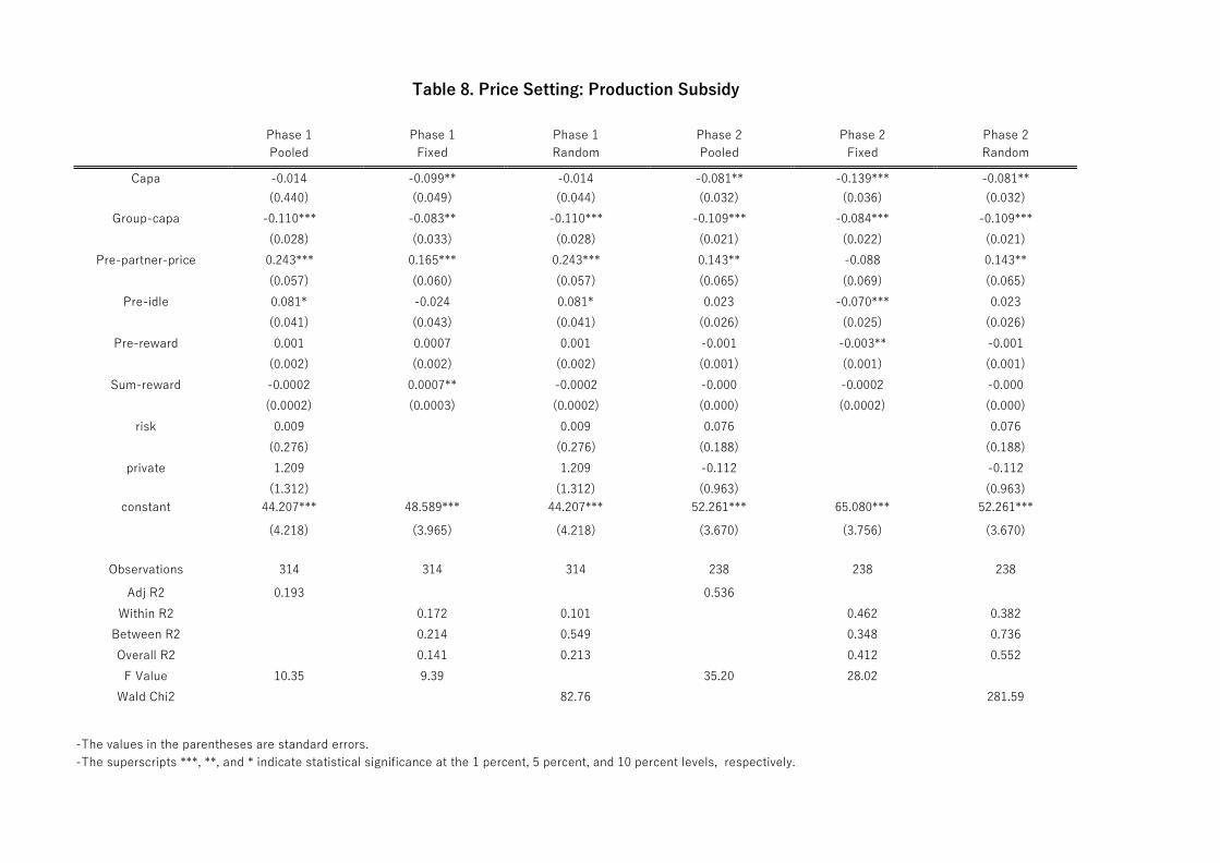
The results for the case of production subsidy and capacity subsidy are shown in Tables 8

and 9, respectively. First, let us examine the effects of changes in capacities. When focusing

on the coefficients of group-capa, all coefficients are significant and negative for both phases

in both cases of subsidies. This result is intuitive and reveals that subjects understand that the

19

total sales and equilibrium prices are negatively correlated.11 However, there is an important

difference in the size of the effect of group-capa between the cases for both types of subsidies.

In the case of a production subsidy, the sizes of the coefficients are almost the same for both

phases. On the other hand, the size of the coefficients for Phase 2 is greater than that for Phase

1 in the case of a capacity subsidy. Moreover, the coefficients of capa is significant and

negative in the case of a production subsidy while, surprisingly, the coefficient is significant

and positive in the case of a capacity subsidy. It is also verified from the coefficients of these

two variables in Phase 2 that (i) a price decrease set by a subject in response to an increase in

her/his own capacity is almost the same between types of subsidies, while (ii) a price decrease

in response to an increase in the partner’s capacity is much greater in the case of capacity

subsidy than in the case of production subsidy. These results imply that subjects respond to

partners’ decisions more aggressively in the case of a capacity subsidy than in the case of

production subsidy. Because private firms decrease their capacities in the first stage when a

capacity subsidy is provided to SOEs, they have a strong incentive to prevent their capacities

from being idle in Phase 2, in particular.

To interpret the difference, we also look at the coefficients of other variables. The

coefficients of pre-partner-price in the case of production subsidy are significant and positive

in Phase 1, which implies that conditional cooperation holds. A subject responds to an increase

in the partner’s price in the previous round by increasing her/his capacity in the present round.

However, the result of the fixed-effects-model estimation is not significant in Phase 2.

Although the results are significant for the other two estimations, the sizes are smaller in Phase

2 than in Phase 1. The situation in the case of a capacity subsidy was different. The coefficients

11 It may be obvious for students of department of economics and business school as far as they are sitting in the lecture room. However, the instruction is a little complicated because they make decisions twice: capacity and price. Moreover, students for other departments are sometimes unfamiliar with this relationship. Thus, this point is important in terms of experimental analysis.

20

of pre-partner-price were insignificant for all estimations in Phase 1, while those of the

pooled-cross-section and random-effects-model estimations were significant and positive in

Phase 2. The sizes of those coefficients were clearly larger in Phase 2 than in Phase 1. Thus, a

subject responded to an increase in the partner’s price in the previous round by increasing

her/his capacity in the present round in Phase 2. In total, it can be said that a capacity subsidy

strengthens conditionally cooperative behavior, while a production subsidy weakens the

behavior. Because the total capacities increase in the case of a production subsidy in Phase 2,

it is natural that the subjects act non-cooperatively.

3.5 Additional Treatments

In this subsection, we examine the results of additional treatments. Because the sample sizes

are relatively small for these additional treatments, we focus only on the averages. The average

capacities, prices, sales, profits, and idle capacities for private firms and SOEs are shown in

Tables 10a and 10b, respectively. Those values in Tables 3 and 4 are the basis of comparison.

Overall, the results depend not on the starting level of the production subsidy but on the

absolute level.

As far as capacities of private firms, there are no large differences between treatments.

However, the direction of the change in capacities and sales of private firms in SS5 and SS9

caused by an increase in the production subsidy is different from the direction in SS1 and SS3.

Capacities and sales in Phase 2 are a little smaller than those in Phase 1. The possible reason

is that SOEs are more aggressive in Phase 2 in SS5 and SS9 than in SS1 and SS3, so private

firms decrease their capacities. On the other hand, the capacities of the SOEs in Phase 1 in SS9

are greater than those in the other treatments. It is possible that there is a threshold: SOEs have

a stronger incentive to increase their capacities when subsidy exceeds the threshold. Similar

results are obtained for sales. The increased amounts of capacities and sales in

21

response to an increase in production subsidy seem to depend not on the increased amounts of

subsidies but on the fact that subsidies are increased or the absolute level of subsidies.

Prices in these additional treatments are not different from those in SS3. However, as long

as we focus on the additional treatments, the amount of subsidy influences the price settings

of both private firms and SOEs. There is no clear difference in prices between SS1 and SS5.

On the other hand, prices in SS9 are clearly lower than those in the other treatments. Similar

results are obtained for profits. The profits of both private firms and SOEs in SS9 are clearly

smaller than those in the other treatments, including SS3. In SS9, competition between a

private firm and an SOE is severe and, accordingly, prices are low and profits are small.

Finally, the result for idle capacities of private firms is interesting. It is likely that the larger

the amount of production subsidy, the greater the amount of idle capacities. Because private

firms are not subsidized, the lower limit of price for them is 20. On the other hand, even if

SOEs set their prices lower than 20, they may gain positive rewards. Thus, the condition of

competition is favorable for SOEs in the second stage, and private firms tend to have larger

amounts of idle capacities compared with SOEs.

4. Discussion

The examination of the results of the experiment leads to implications for economic research

and the political arena, as discussed in this section.

First, it is interesting that the effects of a production subsidy on total supply and surpluses

are different from those of capacity subsidy. The main reason for this difference is the behavior

of private firms in choosing capacities. Although the behavior of price setting is different

depending on the types of subsidies, the difference in the behavior in the first stage dominates

the difference in the behavior in the second stage in terms of the effects on surpluses. Because

a capacity subsidy directly encourages capacity building of SOEs, it is a credible threat in the

22

first stage. Therefore, private firms expect that rival firms (SOEs) will certainly increase their

capacities due to an increase in the capacity subsidy and, accordingly, they decrease their

capacities to avoid drastic decreases in prices and profits due to severe competition.

In the case of production subsidy, this situation arises in the second stage because the

production subsidy directly influences the price-setting behavior of SOEs. Private firms

become less aggressive when choosing their prices after production subsidy increases. On the

other hand, decreases in capacities of private firms cannot be observed. Thus, the difference

in the behavior of private firms in the first stage gives rise to the opposite results in the cases

of two types of subsidies.

We also obtained important policy implications. The first point is that even a small amount

of subsidy may influence the variables of both private firms and SOEs drastically. For example,

focusing again on the behavior of SOEs in SS3 (Table 4a), the increased amount of subsidy in

the objective function of the SOEs is equivalent to a decrease in the marginal cost by 4.29. If

we consider a case in which all capacities are used for production and both firms compete with

each other in quantity, the equilibrium capacity for an SOE increases by 2.86, theoretically.

However, according to the result, the average sales increases by more than 10 units (from

61.394 to 71.635). Moreover, the average sales of private firms also increase, even though the

marginal sales cost is higher after an increase in the SOEs’ production subsidy than before the

increase. Because the experiment results indicate that the production subsidy in SS3 increases

social and domestic surpluses, this subsidy seems to be a desirable policy. However, it is

difficult to know the appropriate amount of production/capacity subsidy to apply. Moreover,

it is likely that subsidies are provided excessively for political reasons. In such a case, when

considering the possibility of drastic changes in capacities and prices, these types of subsidies

should not be allowed easily.

Second, the profits of private firms always decrease in the case of a production subsidy,

23

and an increase in subsidy makes an unfavorable situation for private firms more serious.

Consider a situation in which SOEs are domestic firms and private firms are foreign firms.

Production subsidies for SOEs is then likely to causes an international dispute among trading

countries. Thus, in terms of free and fair competition, production subsidies for SOEs should

be permitted under strict conditions.

Third, the effect of a capacity subsidy is likely to be opposite to the effect of production

subsidy. If the competition structure does not change, capacity subsidy is more detrimental to

profits and surplus because managers of SOEs gain from increases in capacities even if those

capacities are not used for production. They have incentives to increase their capacities, which

is likely to lead to an increase in idle capacity. If the competition for capacity building in the

first stage or price competition in the second stage becomes severe due to an increase in

capacity subsidy, idle capacities of private firms also increase. However, the experiment results

indicate the opposite situation: idle capacities of SOEs do not change and those of private firms

significantly decrease on average. Moreover, as long as the focus is on the average profit, the

increased amount for private firms is greater than that for SOEs. Thus, a capacity subsidy can

be less harmful to profits than a production subsidy as long as the amounts of subsidies are not

very large. However, this situation arises because private firms decrease their capacities in

response to increases in expected capacities of SOEs. On the other hand, if the amount of

capacity subsidy is large, the situation may also be similar to that of production subsidy.12

Consequently, even if the subsidy is provided, the type and volume should be carefully

examined. For example, when the amount of subsidy is small, a production subsidy is more

desirable than a capacity subsidy, because the positive effect on surpluses is likely to dominate

the negative effect on inefficiency like an increase in idle capacities.

12 We did not have enough budget this time to examine the volume effect of capacity subsidy. However, this point is interesting. It is a future task to carry out in additional sessions.

24

However, when the amount of subsidy is relatively large, a capacity subsidy is more desirable

than a production subsidy, because it is less likely that a capacity subsidy will trigger drastic

price decreases.

5. Conclusion

We have experimentally examined whether subsidies for an SOE changes the behavior of

either a private firm or the SOE under mixed duopoly. We conducted a series of laboratory

experiments adopting a two-stage capacity-price decision-making duopoly setting. We

adopted two treatments in terms of types of subsidies: one is a subsidy for production/sales

and the other is a subsidy for capacity building.

We obtained several interesting results. For example, a production subsidy increases the

capacities of both private firms and SOEs and, accordingly, the prices of both types of firms

decrease. On the other hand, a capacity subsidy decreases the capacities of private firms, while

those of SOEs increase. We also found that both social and domestic surpluses increase in the

case of a production subsidy, but decrease in the case of capacity subsidy. In the former case,

the severe competition mitigates the distortion caused by imperfect competition. Moreover,

firm/personal attributes significantly influence capacity choices. In particular, the participant’s

role as a private firm or an SOE significantly influences capacity choices. In summary, the

effects on capacities, prices, sales, idle capacities, and profits depend on the type of subsidy.

The fact that even a small amount of subsidy may substantially influence the variables of

both private firms and SOEs has important policy implications. In some cases, private firms

compete with SOEs in very unfavorable situations. In particular, when foreign private firms

enter the domestic market, even a small amount of subsidy for domestic SOEs may cause an

international dispute. In such a case, the use of subsidies for SOEs should be strictly restricted.

In addition to theoretical analyses in the literature, we believe that we have provided

25

experimental evidence of the effect of subsidies on the situation of mixed duopoly, including

changes in the competition structure and strategic behavior.

References

Chang, W. W. (2007). Optimal trade, industrial, and privatization policies in a mixed duopoly

with strategic managerial incentives. Journal of International Trade and Economic

Development 16, 31-52.

Davis, D. (1999). Advance production and Cournot outcomes: an experimental investigation.

Journal of Economic Behavior and Organization 40, 59-79. Du, N., J. S. Heywood, G. Ye (2013). Strategic delegation in an experimental mixed duopoly.

Journal of Economic Behavior and Organization 87, 91-100.

Durham, Y., K. McCabe, M. Olson, S. Rassenti, V. Smith (2004). Oligopoly competition in

fixed cost environments. International Journal of Industrial Organization 22, 147-162.

Goodwin, D., S. Mestelman (2010). A note comparing the capacity setting performance of the

Kreps-Scheinkman duopoly model with the Cournot duopoly model in a laboratory setting.

International Journal of Industrial Organization 28, 522-525.

Hampton, K., K. Sherstyuk (2012). Demand shocks, capacity coordination, and industry

performance: lessons from an economic laboratory. RAND Journal of Economics 43, 139-

166.

Ishibashi, K., T. Kaneko (2008). Partial privatization in mixed duopoly with price and quality

competition. Journal of Economics 95, 213-231.

Kitahara, M., T. Matsumura (2013). Mixed duopoly, product differentiation, and competition.

Manchester School 81, 730-744. Kreps, D., J. Scheinkman (1983). Quantity precommitment and Bertrand competition yield

Cournot outcomes. Bell Journal of Economics 14, 326-227.

26

Lee, S., L. Xu, Z. Chen (2013). Competitive privatization and tariff policies in an international

mixed duopoly. Manchester School 81, 763-779.

Lu, Y., S. Poddar (2006). The choice of capacity in mixed duopoly under demand uncertainty.

Manchester School 74, 266-272. Luo, J. (2013). Absorptive capacity and R&D strategy in mixed duopoly with labor-managed

and profit-maximizing firms. Economic Modelling 31, 433-439.

Matsumura, T. (1998). Partial privatization in mixed duopoly. Journal of Public Economics

70, 473-483. Matsumura, T. (2003). Endogenous role in mixed markets: A two-production-period model.

Southern Economic Journal 70, 403-413.

Matsumura, T. (2012). Welfare consequence of an asymmetric regulation in a mixed Bertrand

duopoly. Economics Letters 115, 94-96.

Matsumura, T., N. Matsushima (2004). Endogenous cost differentials between public and

private enterprises: A mixed duopoly approach. Economica 71, 671-688.

Muren, A. (2000). Quantity precommitment in an experimental oligopoly market. Journal of

Economic Behavior and Organization 41, 147-157.

Nie, P. (2014). Effects of capacity constraints on mixed duopoly. Journal of Economics 112,

283-294.

Ohnishi, K. (2008). International mixed duopoly and strategic commitments. International

Economics and Economic Policy 4, 421-432.

Ohnishi, K. (2009). Capacity investment and mixed duopoly with state-owned and labor-

managed firms. Annals of Economics and Finance 10, 49-64.

Ou, R., J. Li, J. Lu, C. Guo (2016). The optimal privatization policy under an international

mixed duopoly. Review of Development Economics 20, 228-238.

Scrimitore, M. (2014). Quantity competition vs. price competition under optimal subsidy in a

27

mixed duopoly. Economic Modelling 42, 166-176. Tomaru, Y., Y. Nakamura, M. Saito (2011). Strategic managerial delegation in a mixed duopoly

with capacity choice: partial delegation or full delegation. Manchester School 79, 811-838.

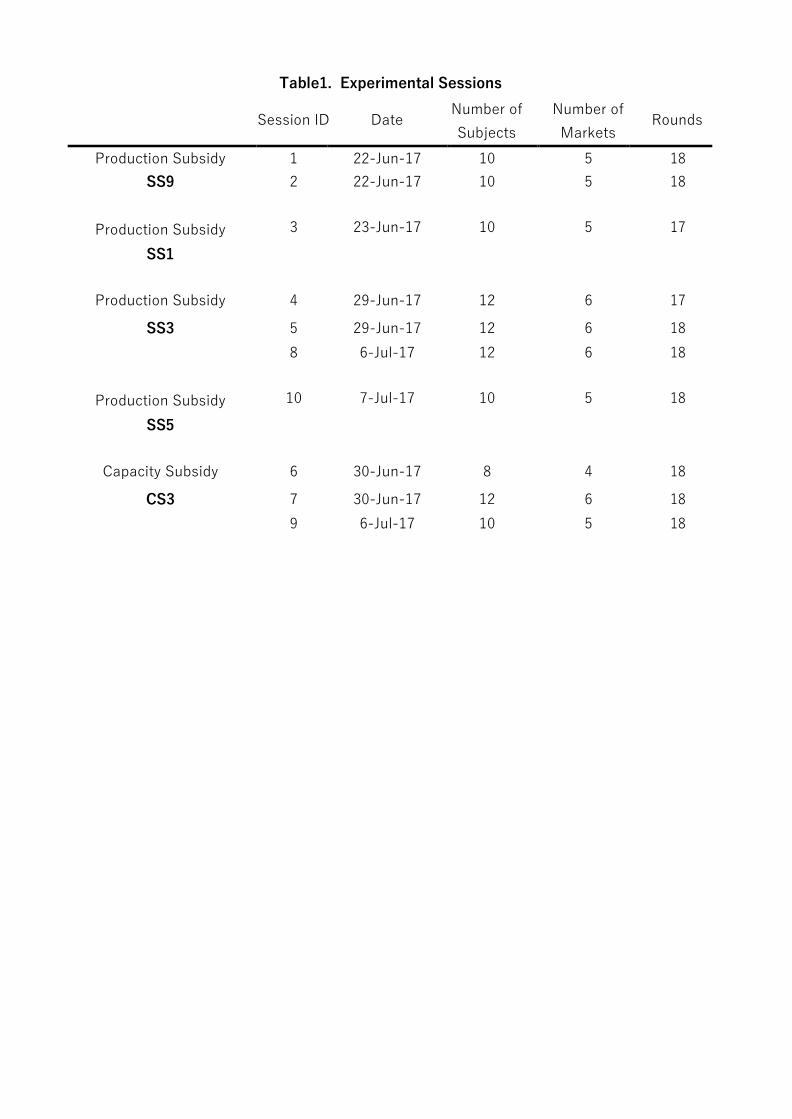
Table1. Experimental Sessions

Session ID Date Rounds Number of Number of Subjects Markets

Production Subsidy 1 22-Jun-17 10 5 18 SS9 2 22-Jun-17 10 5 18

Production Subsidy SS1

3 23-Jun-17 10 5 17

Production Subsidy 4 29-Jun-17 12 6 17

SS3 5 29-Jun-17 12 6 18 8 6-Jul-17 12 6 18

Production Subsidy SS5

10 7-Jul-17 10 5 18

Capacity Subsidy 6 30-Jun-17 8 4 18

CS3 7 30-Jun-17 12 6 18 9 6-Jul-17 10 5 18

Table 2.Wilcoxon Signed-Ranks Test Between Phases for Market Values (P-Values)

Session ID Capacity Price Sales Profits

4 0.040 7.042e-05 0.051 0.021 5 0.475 0.157 0.400 0.300 8 0.172 0.022 0.340 0.438

6 0.399 0.101 0.430 0.077

7 0.582 0.554 <2.2e-16 0.791 9 0.438 0.918 0.956 0.908

Table 3a. Average and Standard Deviations of Private Firm Variables

Ave Phase 1

StDev

Ave Phase 2

StDev

Production Subsidy Capacity 68.128 26.719 71.27 27.371 Price 38.368 10.444 34.635 9.617 Sales 53.776 28.094 55.579 27.167 Profits 531.832 899.039 377.817 955.242 Idle 14.352 29.18 15.69 31.666 Capacity Subsidy Capacity 70.611 27.885 61.712 22.05 Price 35.968 12.008 36.221 9.405 Sales 55.011 24.697 51.587 18.853 Profits 402.211 800.947 567.923 682.205 Idle 16 26.289 10.125 19.9

Table 3b.Wilcoxon Signed-Ranks Test for Private Firm Variables Between Phases (P-Values)

Treatment Capacity Price Sales Idle Profits

Production Subsidy 0.498 0.001 0.281 0.724 0.0096

Capacity Subsidy 0.047 0.857 0.487 0.035 0.211

Table 4a. Average and Standard Deviations of SOE Variables Phase 1 Phase 2

Ave StDev Ave StDev Production Subsidy Capacity 75.096 24.836 83.627 27.506 Price 38.282 10.152 33.611 9.79 Sales 61.394 27.327 71.635 30.629 Profits 696.979 873.746 549.032 931.046 Idle 12.752 21.925 11.992 21.943 Capacity Subsidy Capacity 80.137 25.445 83.596 25.415 Price 35.768 10.113 37.692 11.098 Sales 66.811 25.396 69 23.544 Profits 643.905 836.643 755.096 738.832 Idle 14.073 22.834 14.596 19.857

Table 4b.Wilcoxon Signed-Ranks Test for SOE Variables Between Phases (P-Values)

Treatment Capacity Price Sales Idle

Production Subsidy 0.0005 9.585e-08 7.574e-05 0.991

Capacity Subsidy 0.082 0.537 0.484 0.503

Table 5a. Aerages and Standard Deviations of Surpluses

Phase Ave StDev Production Subsidy Surplus 1 5835.333 469.025 2 6032.732 350.542 Domestic Surplus 1 5288.728 1086.989 2 5654.915 1113.291 Capacity Subsidy Surplus 1 5916.408 459.342 2 5903.642 438.661 Domestic Surplus 1 5514.197 1022.783 2 5335.719 984.325

Table 5b.Wilcoxon Signed-Ranks Test for Surpluses Between Phases (P-Values)

Treatment Surplus Domestic Surplus Production Subsidy 0.0005 0.006

Capacity Subsidy 2.003e-06 0.663

-The values in the parentheses are standard errors. -The superscripts ***, **, and * indicate statistical significance at the 1 percent, 5 percent, and 10 percent levels, respectively.

Table 6. Capacity Choice: Production Subsidy

Phase 1 Pooled

Phase 1 Fixed

Phase 1 Random

Phase 2 Pooled

Phase 2 Fixed

Phase 2 Random

Pre-partner-capa 0.284*** 0.047 0.196*** -0.016 0.090 0.045 (0.066) (0.068) (0.066) (0.095) (0.113) (0.100)

Pre-partner-price -0.171 -0.113 -0.099 -0.568** -0.074 -0.309 (0.120) (0.110) (0.114) (0.221) (0.251) (0.228)

Pre-idle 0.377*** 0.141* 0.252*** 0.068 -0.010 0.012 (0.088) (0.082) (0.084) (0.090) (0.091) (0.869)

Pre-reward 0.014*** 0.009*** 0.011*** 0.004 0.002 0.003 (0.004) (0.003) (0.003) (0.005) (0.005) (0.004)

Sum-reward -0.002*** 0.001* -0.001*** -0.002*** -0.0005 -0.002*** (0.0004) (0.0005) (0.0004) (0.0002) (0.0008) (0.0002)

risk -0.562 -0.474 -0.900 -0.881

private

constant

(0.585) -10.207***

(2.728) 61.327***

61.788***

(0.933) -9.024** (4.395)

63.219***

(-0.630) -15.183***

(3.014) 121.090***

75.814***

(0.962) -16.238***

(4.595) 108.731***

(9.262) (7.953) (10.463) (13.507) (16.880) (15.400)

Observations 314 314 314 238 238 238

Adj R2 0.242 0.364 Within R2 0.046 0.003 0.007 0.004

Between R2 0.335 0.594 0.414 0.622 Overall R2 0.066 0.244 0.260 0.378

F Value 15.28 2.65 10.35 0.29 Wald Chi2 26.22 55.81


Table 7. Capacity Choice: Capacity Subsidy

Phase 1 Pooled

Phase 1 Fixed

Phase 1 Random

Phase 2 Pooled

Phase 2 Fixed

Phase 2 Random

Pre-partoner-capa 0.264*** 0.203** 0.272*** -0.030 0.104 0.022 (0.083) (0.083) (0.080) (0.127) (0.127) (0.124)

Pre-partner-price -0.062 0.300* 0.138 -0.895*** -0.243 -0.635*** (0.169) (0.164) (0.163) (0.216) (0.227) (0.215)

Pre-idle 0.159 0.031 0.094 0.263** 0.150 0.221* (0.114) (0.115) (0.112) (0.127) (0.127) (0.124)

Pre-reward 0.006 0.003 0.004 0.014* 0.010 0.013* (0.005) (0.005) (0.005) (0.007) (0.007) (0.007)

Sum-reward -0.002*** 0.000 -0.0014** -0.001*** -0.0003 -0.001*** (0.001) (0.001) (0.0007) (0.0003) (0.0008) (0.0003)

risk -0.269 -0.222 -0.057 -0.063

private

constant

(0.504) -10.943***

(3.148) 64.826***

45.872***

(0.772) -11.644**

(4.732) 55.673***

(0.515) -14.290***

(3.567) 110.433***

68.324***

(0.675) -16.304***

4.463) 99.460***

(10.805) (10.566) (11.169) (15.314) (16.596) (15.383)

Observations 245 245 245 208 208 208

Adj R2 0.203 0.278 Within R2 0.044 0.016 0.015 0.011


F Value 9.86 1.93 12.36 0.53 Wald Chi2 25.10 47.34


Table 8. Price Setting: Production Subsidy

Phase 1 Pooled

Phase 1 Fixed

Phase 1 Random

Phase 2 Pooled

Phase 2 Fixed

Phase 2 Random

Capa -0.014 -0.099** -0.014 -0.081** -0.139*** -0.081** (0.440) (0.049) (0.044) (0.032) (0.036) (0.032)

Group-capa -0.110*** -0.083** -0.110*** -0.109*** -0.084*** -0.109*** (0.028) (0.033) (0.028) (0.021) (0.022) (0.021)

Pre-partner-price 0.243*** 0.165*** 0.243*** 0.143** -0.088 0.143** (0.057) (0.060) (0.057) (0.065) (0.069) (0.065)

Pre-idle 0.081* -0.024 0.081* 0.023 -0.070*** 0.023 (0.041) (0.043) (0.041) (0.026) (0.025) (0.026)

Pre-reward 0.001 0.0007 0.001 -0.001 -0.003** -0.001 (0.002) (0.002) (0.002) (0.001) (0.001) (0.001)

Sum-reward -0.0002 0.0007** -0.0002 -0.000 -0.0002 -0.000 (0.0002) (0.0003) (0.0002) (0.000) (0.0002) (0.000)

risk 0.009 0.009 0.076 0.076 (0.276) (0.276) (0.188) (0.188)

private 1.209 1.209 -0.112 -0.112

constant (1.312)

44.207***

48.589*** (1.312)

44.207*** (0.963)

52.261***

65.080*** (0.963)

52.261***

(4.218) (3.965) (4.218) (3.670) (3.756) (3.670)

Observations 314 314 314 238 238 238

Adj R2 0.193 0.536 Within R2 0.172 0.101 0.462 0.382


F Value 10.35 9.39 35.20 28.02 Wald Chi2 82.76 281.59


Table 9. Price Setting: Capacity Subsidy

Phase 1 Pooled

Phase 1 Fixed

Phase 1 Random

Phase 2 Pooled

Phase 2 Fixed

Phase 2 Random

Capa 0.033 0.014 0.033 0.086*** 0.111*** 0.086*** (0.035) (0.040) (0.035) (0.029) (0.035) (0.029)

Group-capa -0.178*** -0.183*** -0.178*** -0.279*** -0.289*** -0.279*** (0.025) (0.029) (0.025) (0.020) (0.024) (0.020)

Pre-partner-price 0.025 -0.002 0.025 0.201*** 0.078 0.201*** (0.061) (0.070) (0.061) (0.064) (0.070) (0.064)

Pre-idle 0.116*** 0.012 0.116*** 0.052* -0.010 0.052* (0.040) (0.046) (0.040) (0.030) (0.032) (0.030)

Pre-reward 0.005*** 0.002 0.005*** -0.001 -0.0003 -0.001 (0.002) (0.002) (0.002) (0.001) (0.002) (0.001)

Sum-reward -0.0002 -0.0001 -0.0002 -0.0003*** -0.000 -0.0003*** (0.0002) (0.0003) (0.0002) (0.0001) (0.000) (0.0001)

risk 0.130 0.130 0.036 0.036 (0.183) (0.183) (0.147) (0.147)

private 0.131 0.131 -0.481 -0.481

constant (1.159)

54.863***

61.498*** (1.159)

54.863*** (1.065)

65.860***

68.916*** (1.065)

65.860***

(3.809) (4.006) (3.809) (3.541) (3.845) (3.541)

Observations 245 245 245 208 208 208

Adj R2 0.408 0.642 Within R2 0.257 0.234 0.574 0.555


F Value 21.99 12.07 38.57 Wald Chi2 175.94 379.83

Table 10a. Average Variables for Private Firms for Additional Sessions

SS1 SS5 SS9 Phaes 1 Phase 2 Phaes 1 Phase 2 Phaes 1 Phase 2

Production Subsidy Capacity 66.388 75.848 71.9 71.15 72.826 70.87 Price 39.02 39.788 41.08 38.225 35 34.174 Sales 50.694 41.364 56.44 53.8 55.884 51.174 Profits 463.388 -52.545 625.5 384.5 389.014 207.304 Idle 15.694 33.471 15.46 17.35 16.942 19.696

Table 10b. Average Variables for SOEs for Additional Sessions

SS1 SS5 SS9

Phaes 1 Phase 2 Phaes 1 Phase 2 Phaes 1 Phase 2

Production Subsidy Capacity 75.898 89.848 71.14 81 81.29 87.493 Price 38.939 36.394 40.46 36.1 35.464 32.304 Sales 65.02 78.182 53.78 67.825 67.333 76.377 Profits 736.429 711.212 496.76 455.525 445.899 516.754 Idle 10.878 11.667 17.36 13.175 13.957 11.116

Figure 1: Demand Table

Price Market Demand Price Market Demand 0 200 51 98 1 198 52 96 2 196 53 94 3 194 54 92 4 192 55 90 5 190 56 88 6 188 57 86 7 186 58 84 8 184 59 82 9 182 60 80 10 180 61 78 11 178 62 76 12 176 63 74 13 174 64 72 14 172 65 70 15 170 66 68 16 168 67 66 17 166 68 64 18 164 69 62 19 162 70 60 20 160 71 58 21 158 72 56 22 156 73 54 23 154 74 52 24 152 75 50 25 150 76 48 26 148 77 46 27 146 78 44 28 144 79 42 29 142 80 40 30 140 81 38 31 138 82 36 32 136 83 34 33 134 84 32 34 132 85 30 35 130 86 28 36 128 87 26 37 126 88 24 38 124 89 22 39 122 90 20 40 120 91 18 41 118 92 16 42 116 93 14 43 114 94 12 44 112 95 10 45 110 96 8 46 108 97 6 47 106 98 4 48 104 99 2 49 102 100 0 50 100

Figure 2: Questions for Risk Preferences

Date: Time:

ID

1

ChoiceA ChoiceB Ball Prize Ball Prize

①、②、③ ④、⑤、⑥、⑦、⑧、⑨、⑩

JPY 400 JPY 100

① ②、③、④、⑤、⑥、⑦、⑧、⑨、⑩

JPY 680 JPY 50

2


①、②、③ ④、⑤、⑥、⑦、⑧、⑨、⑩

JPY 400 JPY 100

① ②、③、④、⑤、⑥、⑦、⑧、⑨、⑩

JPY 750 JPY 50

3


①、②、③ ④、⑤、⑥、⑦、⑧、⑨、⑩

JPY 400 JPY 100

① ②、③、④、⑤、⑥、⑦、⑧、⑨、⑩

JPY 830 JPY 50

4


①、②、③ ④、⑤、⑥、⑦、⑧、⑨、⑩

JPY 400 JPY 100

① ②、③、④、⑤、⑥、⑦、⑧、⑨、⑩

JPY 930 JPY 50

5


①、②、③ ④、⑤、⑥、⑦、⑧、⑨、⑩

JPY 400 JPY 100

① ②、③、④、⑤、⑥、⑦、⑧、⑨、⑩

JPY 1060 JPY 50

6


①、②、③ ④、⑤、⑥、⑦、⑧、⑨、⑩

JPY 400 JPY 100

① ②、③、④、⑤、⑥、⑦、⑧、⑨、⑩

JPY 1250 JPY 50

7


①、②、③ ④、⑤、⑥、⑦、⑧、⑨、⑩

JPY 400 JPY 100

① ②、③、④、⑤、⑥、⑦、⑧、⑨、⑩

JPY 1500 JPY 50

8


①、②、③ ④、⑤、⑥、⑦、⑧、⑨、⑩

JPY 400 JPY 100

① ②、③、④、⑤、⑥、⑦、⑧、⑨、⑩

JPY 1850 JPY 50

9


①、②、③ ④、⑤、⑥、⑦、⑧、⑨、⑩

JPY 400 JPY 100

① ②、③、④、⑤、⑥、⑦、⑧、⑨、⑩

JPY 2200 JPY 50

10


①、②、③ ④、⑤、⑥、⑦、⑧、⑨、⑩

JPY 400 JPY 100

① ②、③、④、⑤、⑥、⑦、⑧、⑨、⑩

JPY 3000 JPY 50

Figure 3. Market Values of SS3 Treatments (Production subsidy after round 10)

Average Market Capacity

200 180 160 140 120 100

1 2 3 4 5 6 7 8 9 10 11 12 13 14 15 16 17 18

session 4 Session 5 Session 8

Average Price

50

45

40

35

30

25 1 2 3 4 5 6 7 8 9 10 11 12 13 14 15 16 17 18

Average Market Sales 150 140 130 120 110 100

90 1 2 3 4 5 6 7 8 9 10 11 12 13 14 15 16 17 18

Figure 4. Market Values of SC3 Treatments (Capacity subsidy after round 10)

Average Market Capacity 200 150 100

50

1 2 3 4 5 6 7 8 9 10 11 12 13 14 15 16 17 18

Session 6 Session 7 Session 9

Average Prices

50

45

40

35

30

25 1 2 3 4 5 6 7 8 9 10 11 12 13 14 15 16 17 18

Average Market Sales

150

100

50

1 2 3 4 5 6 7 8 9 10 11 12 13 14 15 16 17 18

subsidies to public firms and competition modes under a ... · subsidies to public firms and...

Documents