substorm injections pr oduce sufficient electr on

Substorm injections produce sufficient electron energization to

account for MeV flux enhancements following some storms

M. J. Mithaiwala and W. HortonDepartment of Physics, University of Texas, Austin, Texas, USA

Received 29 March 2004; revised 9 December 2004; accepted 3 March 2005; published 22 July 2005.

[1] One of the main questions concerning radiation belt research is the origin of very highenergy (>1 MeV) electrons following many space storms. Under the hypothesis that theplasma sheet electron population is the source of these electrons, which are convected tothe outer radiation belt region during substorms, we estimate the flux of particlesgenerated at geosynchronous orbit. We use the test particle method of following guidingcenter electrons as they drift in the electromagnetic fields during substorm dipolarization.The dipolarization pulse model electromagnetic fields are taken from the Li et al. (1998)substorm particle injection model. We find that a substorm dipolarization can produceenough electrons within geosynchronous orbit to account for the electrons seen followingstorms. To do this, we compute transport ratios of plasma sheet electrons, that is, therelative ratio of plasma sheet electrons that are transported and trapped in the innermagnetosphere during substorms, as well as the change in energy of the electrons. Sincehigh fluxes of MeVelectrons are only seen following storms and not isolated substorms, itis likely that these electrons may serve as a source population for other energizationmechanisms which accelerate the electrons to MeV energies. Furthermore, we doparametric studies of the dipolarization model to understand physically what conditionsenable the generation of this source population.

Citation: Mithaiwala, M. J., and W. Horton (2005), Substorm injections produce sufficient electron energization to account for MeVflux enhancements following some storms, J. Geophys. Res., 110, A07224, doi:10.1029/2004JA010511.

1. Introduction

[2] One of the main questions concerning current spaceweather research is the origin of the relativistic electronradiation belts existing in the dipolar regions of the Earth’smagnetosphere. Given that the average electron temper-atures of solar and magnetospheric particles are Te !10 eV for the solar wind, 30 eV in the magnetosheath,500 eV in the plasma sheet, and less than 1 eV in theionosphere, it is important to ask what is the means thatthese low-energy electrons come to be energized to 1 MeVand above in the radiation belts. Baker et al. [1998] proposethat that the process by which high-energy (>1 MeV)electrons are accelerated is twofold: first, there is a promptacceleration of electrons during magnetospheric substormsand, second, involves other acceleration mechanismsthroughout the trapping region (the region in the innermagnetosphere where electrons and ions can drift on closedshells) on a timescale of days. Our focus here is on the firststep of this process. The issue of whether the particles comefrom the solar wind has been addressed in the work of Li etal. [1997]. It was determined that the phase space density ofsolar wind electrons (>20 keV) is not adequate to supply theradiation belts. The plasma sheet is the likely source of

particles. The magnetosheath and ionosphere as sources willnot be considered here.[3] One can ask whether substorms themselves can pro-

duce relativistic outerbelt electrons? This question wasaddressed in the work of Kim et al. [2000]. They traceelectron guiding center test particles in MHD modeledfields. The MHD fields were meant to simulate a dipolari-zation process that occurs during substorm onset. The testparticle traces showed that plasma sheet electron energies oftens of keV can be transported from 20 RE to 10 RE and cangain about a factor of 10 in energy. When the particles werefurther transported (by what was assumed to be diffusion) to6 RE while conserving the first adiabatic invariant, they willhave energies of 1 MeVor greater. Estimating the number ofsource relativistic electrons, they find that only 2% ofradiation belt electrons could be accounted for, althoughthis estimate is very sensitive to electron temperature.Ingraham et al. [2001] report that the March 1991 stormhad intense substorm activity, and velocity dispersion anal-ysis shows that substorms transport not only typical 50–300 keV electrons but also relativistic 0.3 to several MeVelectrons to geosynchronous orbit.[4] Another dipolarization model is the Li et al. [1998]

model. The main result of this model was that it accuratelysimulated a dispersionless injection event seen on 10 January1997. Sarris et al. [2002] revised the Li et al. [1998]model to make the propagation speed of the time-varying

JOURNAL OF GEOPHYSICAL RESEARCH, VOL. 110, A07224, doi:10.1029/2004JA010511, 2005

Copyright 2005 by the American Geophysical Union.0148-0227/05/2004JA010511$09.00

A07224 1 of 16

fields a function of radial distance. This model also repro-duced the timing and flux of dispersionless electrons.[5] We can then ask: ‘‘Is the plasma sheet electron

population the source of radiation belt electrons? Is theresufficient phase space density? How many electrons can betransported efficiently and under what circumstances?’’Since many of the features associated with the Li modelhave already been published and are known, i.e., disper-sionless injections, drift echoes, injection boundaries, thecurrent work reported here is to ask similar questions to Kimet al. [2000] and Ingraham et al. [2001], i.e., what is theflux of electrons at geosynchronous orbit due to theseinjections? Is the flux of particles enough to account forthe high-energy radiation belt particles created by diffusiveprocesses or other in situ heating processes?[6] Previously, Delcourt et al. [1990] and Birn et al.

[1998] have investigated electron injections on the basis oftest-electron orbits in the dynamic fields of a three-dimen-sional MHD simulation of dipolarization. They find resultsin excellent agreement with observations of substorm injec-tions. Zaharia et al. [2000] compute electron orbits analyt-ically and also find agreement with observations ofsubstorm electron fluxes.[7] Recently, an important issue regarding substorm

injections is the relation between single large-scale dipola-rization pulses with multiple smaller-scale pulses. We notethat often there is a series of dipolarizations producing thesawtooth waveform of the injected ion flux. There are manyexamples of saw tooth injections such as the GEM storm for4–6 October 2000 submitted for community-wide study.Ingraham et al. [2001] propose that strong repetitive sub-storm injections during the March 1991 storm contributedsignificantly to the near-record levels of MeV electronfluxes.[8] We begin by describing the Li et al. dipolarization

pulse model, indicating some results that have already beenestablished, followed by simulations of plasma sheet par-ticles. In particular, we reproduce and comment on some ofthe typical features of observed dispersionless injections.Then we determine the effect of the model parameters oftransporting and energizing plasma sheet electrons to theinner magnetosphere, followed by calculations of the flux ofelectrons generated by substorm injections compared withthat seen after a storm.

2. Substorm Dipolarization and Particle Injection

[9] Particle injections at geosynchronous orbit have longbeen a reliable indicator of substorm onset and have longsince been observed [Arnoldy and Chan, 1969]. The injec-tions of electrons are often dispersionless in that the flux ofsoft electrons (<300 keV) are simultaneously enhanced.Although dispersionless ion injections are also observedand may play a very important role in the generation of thering current [Kamide et al., 1998; Daglis et al., 1999], wedo not consider them here.[10] Two different mechanisms have been proposed for

the explanation of these events, a dynamic process suchas transport of particles from other spatial regions orpenetration by a quasi-static spatial structure [Kivelson etal., 1979]. The dispersionless nature of these injectionslead to the ‘‘injection-boundary’’ model, in which a time-

varying spatially localized electric field heats the plasmathrough convective flow. This belongs in the lattercategory [McIlwain, 1974]. Local spatial energizationwas thought to be required since energy dependentgradient drifts r?B would disperse the plasma spatiallyaccording to energy.[11] Russell and McPherron [1973] first reported a com-

pressional pulse associated with dipolarization based onOGO-5 and ATS-1 observations. They suggested that atthe expansion phase onset, cross-tail currents weaken andthis information is carried across field lines as a compres-sional wave toward the Earth. Furthermore, they noted thatthese compressional waves produced ‘‘significant betatronacceleration.’’ The perpendicular flux of particles with 90!pitch angles sharply increased while the parallel fluxremained relatively constant. On the basis that the injectedplasma is associated with an abrupt increase in the magneticfield, Moore et al. [1981] showed that an induced electricfield of the compressional wave is responsible for theinjected particles.[12] Substorm injections typically produce energies up to

a few hundred (!300) keV [Cayton et al., 1989; Baker etal., 1989]. Furthermore, they typically have a ‘‘pancake’’pitch angle distribution, that is, the distribution is stronglypeaked toward 90! [Russell and McPherron, 1973; Baker etal., 1978]. Even the MHD field study of Kim et al. [2000]find that only particles near 90! pitch angle are transportedto the inner magnetosphere. For these reasons we consider itreasonable to only consider 90! pitch angle electrons butstill recognize that it is an approximation.

2.1. Li et al. Model

[13] The Li et al. model is an analytic model for anearthward propagating compressional wave, it is onlymeant, however, to have the necessary electrodynamics toexplain dispersionless injections. However, it can be asso-ciated with the phenomenology of substorm onset. Inparticular, the magnetic field consists of an increase fol-lowed by a decrease with the net effect that the magnitudeof the field is larger, indicating dipolarization. This increas-ing field should also correspond to an increased currentperpendicular to the plane, indicating the rise of the ‘‘sub-storm current wedge’’ and the associated decreased cross-tail current of a ‘‘current disruption.’’ The model does notconsider a background dawn-to-dusk electric field or thecorotation electric field that normally exists in the magne-tosphere. The lack of background convection field maypreclude any accurate calculation of the fluxes of injectedparticles associated with substorms; however, the model hasbeen successful in modeling observed particle injections,although adding a dawn-to-dusk electric field increasesconvection, which would only make the conclusions heremuch easier to attain.[14] This model has its origins in a model for the sudden

compression of the magnetosphere by an interplanetaryshock, in particular that which occurred during the 24 March1991 SSC [Li et al., 1993]. The electric and magnetic fieldsassociated with dipolarization were originally used to modela shock event which suddenly produced a new radiationbelt. Sarris et al. [2002] vary the pulse speed with radialdistance to demonstrate that dispersionless injections areachievable under low propagation speeds. This model is a

A07224 MITHAIWALA AND HORTON: SUBSTORM INJECTION FLUX

2 of 16

A07224

nine parameter model which describes analytic electric andmagnetic fields during a substorm dipolarization.[15] The model fields are most easily derived from the

magnetic vector potential

Af r;f; q ¼ p2

! "

¼ dE0 1þ A cos f$ f0ð Þð Þp

v rð Þ

ffiffiffi

pp

2

' erf x r;f; tð Þ½ ) þ 1f g ð1Þ

using spherical polar coordinates with q = p/2 in theequatorial plane and f = 0! is at local noon, positiveeastward.[16] It is useful to define two variables Ri(f) and x:

Ri fð Þ * Ri þC v rð Þvd

1$ cos f$ f0ð Þð Þ; ð2Þ

x * r $ Ri fð Þ þ v rð Þtd

; ð3Þ

which are the initial radius of the pulse which depends onthe local time f and the location of the peak of the pulsex = 0.[17] The Li et al. model pulse parameters are {Pi} = P =

{E0, d, p, vd, v0, A, C, Ri, f0}.E0 The amplitude of the electric field;d d/

ffiffiffi

2p

is the radial width of the Gaussian pulse;p Controls the longitudinal width of the pulse;v0 The velocity of the pulse;vd Longitudinal pulse velocity;A Controls the asymmetry between the dayside/nightside

amplitude;C Controls the delay to longitudes away from f0 or the

ratio of v0 to vd;

Ri The initial position of the pulse;f0 The modeled electric and magnetic fields are max-

imum at f0.

[18] The electric and magnetic fields are readily obtained:

Ef ¼ $ @Af

@t¼ $E0 1þ A cos f$ f0ð Þð Þp exp $x2

$ %

ð4Þ

Bq ¼ r+ A½ )q¼ $Af

r$ @Af

@rð5Þ

¼ v0 rð Þv2 rð Þ dE0 1þ A cos f$ f0ð Þð Þp

ffiffiffi

pp

2erf xð Þ þ 1ð Þ

$E0 1þ A cos f$ f0ð Þð Þp

v rð Þ 1þ v0 rð Þ t $ C

vd1$ cos f$ f0ð Þð Þ

& '( )

' exp $x2$ %

$ dE0 1þ A cos f$ f0ð Þð Þp

rv rð Þ

ffiffiffi

pp

2erf xð Þ þ 1ð Þ:

The electric field, Figure 1a, is a Gaussian pulse withelectric field vector from the dawn-to-dusk direction. Themagnetic field, Figure 1b, shows an overall increase of jBqjsimulating a dipolarization event, i.e., an increase in thenorthward component of the magnetic field. After thetransient pulse has passed, the magnetic field is increased by

Bq ¼ $ d

r

E0

v rð Þffiffiffi

pp

1þ A cos f$ f0ð Þð Þp ð6Þ

Figure 1b. The dipolarizing magnetic field. This figureshows the pulse propagation along the midnight axis. Morespecifically, each profile represents the magnetic field thatwould be seen by a satellite at 6.6, 11.6, 16.6, 21.6, 26.6 RE.The magnetic field behind the pulse is increased bydr

E0

v rð Þffiffiffi

pp

(1 + A cos(f $ f0))p. The 1/r dependence explainswhy the final field is smaller at larger radii.

Figure 1a. The electric field is a Gaussian pulse thattravels earthward. This figure shows the pulse propagationalong the midnight axis. More specifically, each profilerepresents the electric field that would be seen by a satelliteat 6.6, 11.6, 16.6, 21.6, 26.6 RE. This pulse has parametersE0 = 0.5 mV/m, v0 = 100 km/s, d = 16,000 km , 2.5 RE, p =3, A = 1, B = 4.0, vd = 100 km/s, f0 = 180!. The maximumfield is given by E0 2

p = 4.0 mV/m.


3 of 16

A07224

when the pulse propagation velocity v(r) is constant.Figure 1b also shows the 1/r dependence of the resultingmagnetic field.[19] Further analysis of the field equations, in particular

the (1 + A cos(f $ f0))p, reveals with A = 1 (which is used

throughout this article)

1þ A cos f$ f0ð Þð Þp ¼ 2p cos2p f$ f0ð Þ=2ð Þ

, 2p exp $ p

4f$ f0ð Þ2

! "

: ð7Þ

For this reason, themaximum amplitude of the electric field isreally E0 ' 2p. The exponential dependence on (f$ f0)

2 alsoindicates that the characteristic longitudinal width of thepulse is 2/

ffiffiffi

pp

. A typical substorm current wedge with a 60!angle [McPherron, 1995] would correspond to p = 14.6, butwe have no evidence that the longitudinal width of thesubstorm current wedge has any relation to the width ofthe pulse.[20] These fields are superimposed upon the Earth’s

background field (BE), which is computed using the Tsyga-nenko 96 (T96) model [Tsyganenko and Stern, 1996]. TheT96 model is much more realistic in the sense that a simpledipole field is much stronger near the Earth than theobserved field parameterized by the T96 model. Figure 2shows the strength of the dipole field (dotted line) in theequatorial plane along the midnight axis, the T96 field(dash-dotted line) with parameters Dst = $50.0 nT, Pdyn =3.0 nPa, Bz = $3.0 nT chosen to represent a moderatelyactive magnetosphere, and the total field strength (pulse

field plus the background field) after dipolarization isshown with the solid line. The change in overall strengthfrom a depressed background field to a more dipole likefield indicates dipolarization. It has been verified that r '(BE + Bq) = 0 and Ef ' (BE + Bq) = 0.

3. Particle Motion

[21] For the electromagnetic pulse used in these calcu-lations the space scale variation, s can be estimated by thewidth of the Gaussian pulse, s = d/

ffiffiffi

2p

! 107 m for a widthd ! 1.5 ' 107 and the timescale Dt = s/v0 ! 105 s.Considering electron energies in the range of 10 keV to500 keV found in the magnetotail and magnetic fieldstrengths from 10 nT in the stretched to 200 nT in thedipolar regions (see Figure 2), the gyroradius, re =ffiffiffiffiffiffiffiffiffiffiffiffiffiffiffi

2mWð Þp

/qB, of a typical electron decreases from 250 kmto 2 km and thus s/re > 50 – 1500 and wceDt > 106, wherewce = qB/m is the electron cyclotron frequency. These largeratios show that it is sufficient to use the guiding-centerequations for practical simulations.[22] The equations of motion are determined by the

guiding center equation [Northrop, 1963]

v ¼E$ m

ger?B! "

+ B

B2; ð8Þ

where g = 1 + mBmis the relativistic factor and m = p?

2 /2mBis the first adiabatic invariant or magnetic moment withB(x, t) evaluated at the guiding center x(t). It is essentialthat these equations retain the Hamiltonian structure ofthe system [Littlejohn, 1983] in order that Liouville’stheorem can be applied to obtain the flux withingeosynchronous orbit transported from other regions ofthe magnetosphere. The guiding-center position x is givenby integration:

x tð Þ ¼ x0 t0ð Þ þZ t

t0

dt0v x t0ð Þ; t0ð Þ: ð9Þ

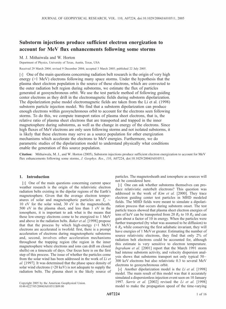
[23] Figure 3a shows two electron orbits under themodel fields. Initially, when there is no electric field,the electrons undergo gradient drift motion; the magneticfield gradient is in the negative radial direction($r̂) andthe magnetic field direction is out of the plane(̂z) so theresulting motion is toward the dawnside(f̂). Whenthe magnetic field of the pulse encounters the electron,the gradient reverses and the electrons begin to drifttoward dusk(f̂). The electric field of the pulse is fromdusk-to-dawn($f̂), so the electron drifts radially towardthe Earth during the encounter with the pulse as well. Asthe pulse passes by the electron, it again begins to drifttoward dawn($f̂).[24] The change in particle kinetic energy (W) is given by

conservation of the magnetic moment m = W/B:

DW ¼ mDB: ð10Þ

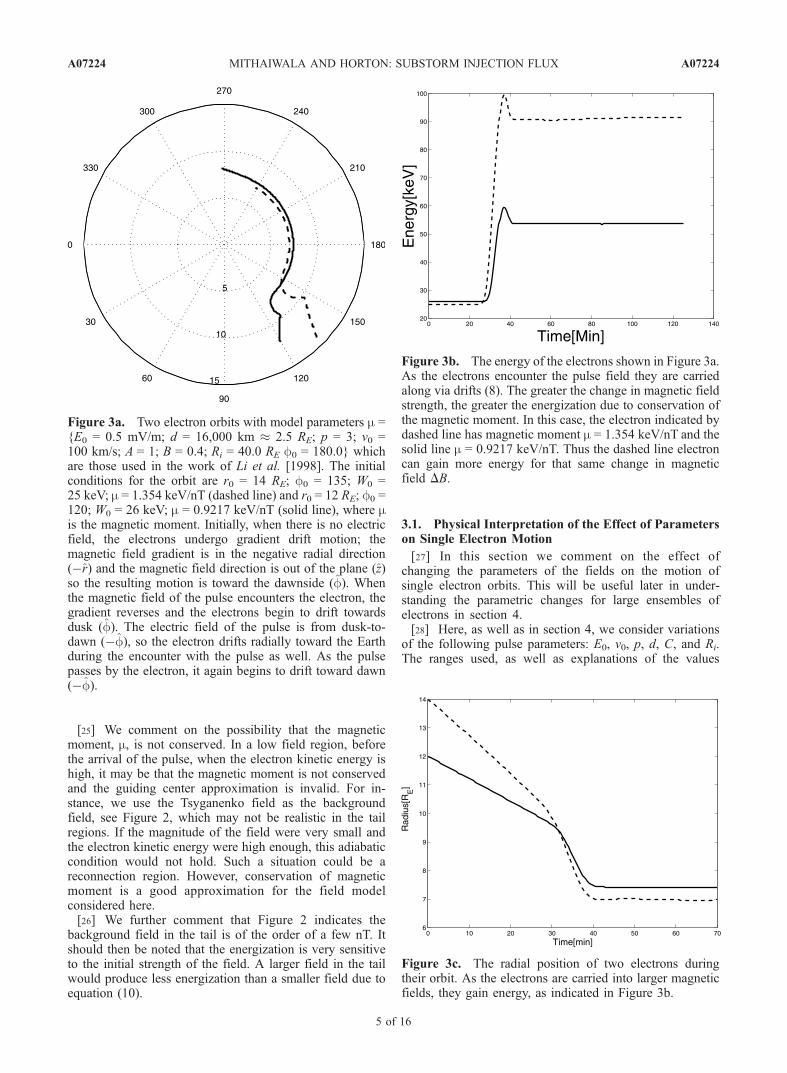
Figure 3b shows the energy of two electrons duringtheir orbits. As the particles are carried radially inward(Figure 3c), they are energized according to (10).

Figure 2. The T96 model is much more realistic in thesense that a simple dipole field is much stronger near theEarth than the T96 model. Here we compare the fieldstrength in the equatorial plane along the midnight axis.The the T96 field with parameters Dst = $50.0 nT, Pdyn =3.0 nPa, Bz = $3.0 nT (dash-dotted line), dipole field(dotted line), the field at time t = 25 min in cyan, and thetotal field strength, i.e., T96 background plus model fields(solid line). The field changes from the background field(dash-dotted line) to the intermediate field (dashed line),and the final field (solid line) after dipolarization. The finalfield is more like a dipole (dotted line) in the innermagnetosphere where we are interested.


4 of 16

A07224

[25] We comment on the possibility that the magneticmoment, m, is not conserved. In a low field region, beforethe arrival of the pulse, when the electron kinetic energy ishigh, it may be that the magnetic moment is not conservedand the guiding center approximation is invalid. For in-stance, we use the Tsyganenko field as the backgroundfield, see Figure 2, which may not be realistic in the tailregions. If the magnitude of the field were very small andthe electron kinetic energy were high enough, this adiabaticcondition would not hold. Such a situation could be areconnection region. However, conservation of magneticmoment is a good approximation for the field modelconsidered here.[26] We further comment that Figure 2 indicates the

background field in the tail is of the order of a few nT. Itshould then be noted that the energization is very sensitiveto the initial strength of the field. A larger field in the tailwould produce less energization than a smaller field due toequation (10).

3.1. Physical Interpretation of the Effect of Parameterson Single Electron Motion

[27] In this section we comment on the effect ofchanging the parameters of the fields on the motion ofsingle electron orbits. This will be useful later in under-standing the parametric changes for large ensembles ofelectrons in section 4.[28] Here, as well as in section 4, we consider variations

of the following pulse parameters: E0, v0, p, d, C, and Ri.The ranges used, as well as explanations of the values

Figure 3a. Two electron orbits with model parameters m ={E0 = 0.5 mV/m; d = 16,000 km , 2.5 RE; p = 3; v0 =100 km/s; A = 1; B = 0.4; Ri = 40.0 RE f0 = 180.0} whichare those used in the work of Li et al. [1998]. The initialconditions for the orbit are r0 = 14 RE; f0 = 135; W0 =25 keV; m = 1.354 keV/nT (dashed line) and r0 = 12 RE; f0 =120; W0 = 26 keV; m = 0.9217 keV/nT (solid line), where mis the magnetic moment. Initially, when there is no electricfield, the electrons undergo gradient drift motion; themagnetic field gradient is in the negative radial direction($r̂) and the magnetic field direction is out of the plane (̂z)so the resulting motion is toward the dawnside (f̂). Whenthe magnetic field of the pulse encounters the electron, thegradient reverses and the electrons begin to drift towardsdusk (f̂). The electric field of the pulse is from dusk-to-dawn ($f̂), so the electron drifts radially toward the Earthduring the encounter with the pulse as well. As the pulsepasses by the electron, it again begins to drift toward dawn($f̂).

Figure 3c. The radial position of two electrons duringtheir orbit. As the electrons are carried into larger magneticfields, they gain energy, as indicated in Figure 3b.

Figure 3b. The energy of the electrons shown in Figure 3a.As the electrons encounter the pulse field they are carriedalong via drifts (8). The greater the change in magnetic fieldstrength, the greater the energization due to conservation ofthe magnetic moment. In this case, the electron indicated bydashed line has magnetic moment m = 1.354 keV/nT and thesolid line m = 0.9217 keV/nT. Thus the dashed line electroncan gain more energy for that same change in magneticfield DB.


5 of 16

A07224

chosen, are given in section 4.1. The background magneticfield for this section is a dipole field because the motion iseasier to compare for the different parameters. Later we usethe more realistic Tsyganenko model.

[29] Figure 4a shows the electron orbit under differentmagnitudes of the electric field. With a stronger electricfield, the electron can gain more energy and will be trans-ported inward further than with a weaker electric field. In

Figure 4. The electron orbit under different variations of the pulse parameters. The electron orbits arecomputed for pulse parameters of P = E0 = 0.5 mV/m, d = 16,000 km , 2.5 RE; p = 3; v0 = vd = 100 km/s;A = 1; C = 0.0 RE; Ri = 40.0 RE; f0 = 180.0 as baseline parameters, while varying each of the otherparameters separately. See color version of this figure at back of this issue.


6 of 16

A07224

addition, during the interval when the electron’s drift isreversed, the electron will drift farther in the dusk direction.[30] Figure 4b shows the electron orbit under different

magnitudes of the velocity of the pulse. The orbit labeledwith v0 = 500 m/s has very little interaction with the electricfield because it moves by so quickly; hence its drift reversaland radial transport is very small. With a smaller velocity,for example v0 = 50 m/s to 200 m/s, the electron interactswith the electric field longer and can drift radially inwardbetter. With a very slow field, the electron drifts azimuthallyaway and does not interact strongly with a large electricfield.[31] Figure 4c shows the electron orbit under different

magnitudes of the longitudinal width, controlled by theparameter p. Large p corresponds to a small width and asmall p corresponds to a large width. For orbits labeled withp = 32 and p = 64, the resulting orbit has a bit of a kinkbetween 180! and 210!. This is a result of the electrondrifting azimuthally out of the electric field. With largerpulse widths, i.e., p = 1.0, 3.0, 8.0, this does not occurbecause the pulses are very wide. Naturally, the widerpulses transport electrons inward further because of thelonger interaction with the electric field.[32] Figure 4d shows the electron orbit under different

magnitudes of the radial width, controlled by the parameterd. Larger d correspond to larger widths and vice versa. Theeffect is clear, larger widths correspond to a longer interac-tion with the fields and hence a better inward transport.

[33] Figure 4e shows the electron orbit under differentinitial positions of the pulse. When the pulse starts very farearthward, i.e., Ri = 10 RE, there is no opportunity for theelectron to interact with the pulse fields. Otherwise, chang-ing the initial position shows that having the pulse startfurther back is better at transporting the electron earthward;however, this shows only one initial condition.[34] Figure 4f shows the electron orbit under different

magnitudes of the azimuthal velocity. A larger value of Cmeans that the pulse is delayed to longitudes away from180!. An electron drifting across many different longitudeshas the opportunity to see many different peaks in theelectric field, as in Figure 4g. So for larger C, the motioncan be very complicated.[35] The results indicate what should be physically clear.

The longer the electron can stay in the fields, the better itwill be at gaining energy. To get an accurate picture ofwhat happens during a substorm, we must consider largernumbers of electrons with a wide range of initial conditions.We do this in section 4.

3.2. Electron Orbits and Electron Fluxes

[36] In the orbit simulations we use the GSM coordinatesand integrate (8) and (9) directly. For understanding theimplications of the simulations for the phase space density fand particle flux J, it is clearer to use canonical coordinatesand the Hamiltonian structure of the guiding-center equa-tions. The standard canonical coordinates for the dynamicsare the magnetic flux y and the longitudinal angle f.Transforming from x, y to y, f, the dynamics are given by

df

dt¼ @f

@tþ f ;H½ ) ¼ 0; ð11Þ

where [H, '] is the directional derivative (Lie derivative)along the y, f orbits

dydt

¼ $ @H

@fdfdt

¼ @H

@yð12Þ

Figure 4g. The electric field as seen by the electrons inFigure 4f. Because the pulse is greatly delayed to longitudesaway from 180! with C = 20.0 RE, the solid line (C =20.0 RE) electron sees a strong electric field many times inits orbit.

Figure 4f. The electron orbit under different magnitudesof the azimuthal velocity. The electron orbit indicated withthe dashed line for parameter C = 1.0 RE and the solid linefor C = 20.0 RE. All other parameters remain constant at P =E0 = 0.5 mV/m; v0 = vd = 100.0 km/s; Ri = 40.0 RE; d =16,000 km , 2.5 RE; p = 3; A = 1; f0 = 180.0. Because thepulse is greatly delayed at longitudes away from 180!, thesolid line electron (C = 20.0 RE) orbit is much morecomplex than the other orbit. As the electron drifts tolongitudes away from 180!, it can interact with the pulsethat is delayed to these longitudes. The electric field seen bythe electrons is shown in Figure 4g.


7 of 16

A07224

and

H ¼ mB y;f; tð Þ ð13Þ

is the Hamiltonian for the flow in the equatorial plane.Clearly, it is the broken symmetry from the f-dependence ofthe electromagnetic pulse that brings the electrons into theinner magnetosphere.[37] The magnetic field B is given in Clebsch form of B =

ry + rf; y and f label a field line and s is the coordinatealong the field line. Similarly, the magnetic field is givenby B = Bdr/ds. Each guiding-center orbit represents anensemble of a very large number of electron orbits in afinite domain (at least pre2 and often much larger) of theequatorial plane. Every area DyDf is conserved by theHamiltonian flow in equations (11)–(13). The inverseJacobian transformation

1

J¼ @ y;f; sð Þ

@ x; y; zð Þ

*

*

*

*

*

*

*

*

¼ rs 'ry+rfj j ¼ rs ' Bj j ¼ B: ð14Þ

Thus the physical area DxDy of a group of electrons aroundeach guiding-center orbit is compressed by (DxDy)tf =DyDf/Bf = (Bi/Bf)(DxDy)ti in the transport from ti to tf,since the Jacobian transformation j@(x, y, z)/@(y, f, s)j = 1/B(14). Assuming no electrons are lost, then the invariance of fmeans that the line density per unit area DxDy increases by(Bf /Bi) in the transport to the inner magnetosphere for thegroup of electrons in the kinetic energy range (Wi, Wi +DWi), where Wi = mBi. This gives the standard relation jf =(pf /pi)

2ji [Lyons and Williams, 1984, p. 21], whichexpresses conservation of phase space density. Their finalspeed, however, is dominated by v? = (mBf)

1/2 and not theguiding center velocity v from (8). So the particle fluxmeasured by a detector in the inner magnetosphere is jf =(Bf /Bi)ji greater than the initial particle flux ji. By therelation W = mB (10),

jf ¼ Wf =Wi

$ %

ji: ð15Þ

[38] Including the compression of the flux tube along thelength s of the magnetic flux tube increases the l exponentsof the compression factors (Bf/Bi)

l. Now we consider sometypical estimates implied by the simulations. Assuming atrajectory from the simulations that takes the bundle ofneighboring electrons along y(t), f(t) to the inner magneto-sphere to orbits with R ! 5, we estimate that the line densityincreases by Bf /Bi ! 250 nT/10 nT = 25.[39] The particle flux is increased by greater than 100 and

less than 500. To reduce the uncertainty in the range of theenhancement factors requires assumptions about the degreeof stretching of the magnetic field lines due to cross-tailcurrent DIgt enclosed between the initial and final fieldlines (‘iBi ffi ‘f Bf + m0DIgt) and the pitch-angle distributionof the high-energy electron velocity distribution.

4. Multiparticle Simulation

[40] Ensembles of electrons can be integrated in order tocompare results with satellite observations and previous

studies. Here we distribute electrons in the equatorial planefrom 7.5 RE . r . 20 RE in increments of 0.1 RE, 0! . f <360! in increments of 1!, and energies from 1 keV . W .512 keV in increments of 1 keV. This corresponds to theintegration of 2,322,4320 electrons. Parallel computer codeallows the simulation to be done swiftly. The lower radialbound was chosen as greater than 7 RE since our virtualdetectors begin at 6.8 RE. These ranges were chosen as to besimilar to the simulation of Li et al. [1998]. The dipolariza-tion field parameters are also those of Li et al. [1998],namely E0 = 0.5 mV/m, v0 = 100 km/s, d = 16,000 km ,2.5 RE, p = 3, A = 1, B = 4.0, vd = 100 km/s, f0 = 180!.[41] The initial electron distribution in the tail is given by

a generalized maxwellian or kappa distribution [Vasyliunas,1968]

j ¼ j01þ 1=kð Þ1þk

Ek

W

1þW=kEkð Þ1þk ; ð16Þ

with k = 3.5, Ek = 1.14 keVand j0 = 5.5 ' 106 cm$2 s$1 sr$1

keV$1 [Christon et al., 1991]. We have chosen theparameters as Kim et al. [2000]. These parameters representa harder spectra that is observed during active conditions.Figure 5 shows the initial flux as would be measured by asatellite in the tail region.[42] By examining the arrival time of the electrons, we

determine that the particles that show appreciable energygains coincide with the arrival of the dipolarization pulse(Figure 6). Figure 8 shows the initial location of theseelectrons as well as the location of the virtual satellites usedas detectors. In keeping with other studies [Li et al., 1998]of a similar nature, we do include a radial dependence in thedistribution,

f ¼ r0 $ a0ð Þnl

rml0

" #,

a0d $ a0ð Þnl

aml0d

" #

ð17Þ

Figure 5. The initial flux of magnetic tail particles ismodeled by a kappa distribution (16). We have chosen theparameters as Kim et al. [2000] with k = 3.5, Ek = 1.14 keVand j0 = 5.5 ' 106 cm$2 s$1 sr$1 keV$1.


8 of 16

A07224

and f = f * exp ($r02/7.52) when r0 > 12 RE. The parameters

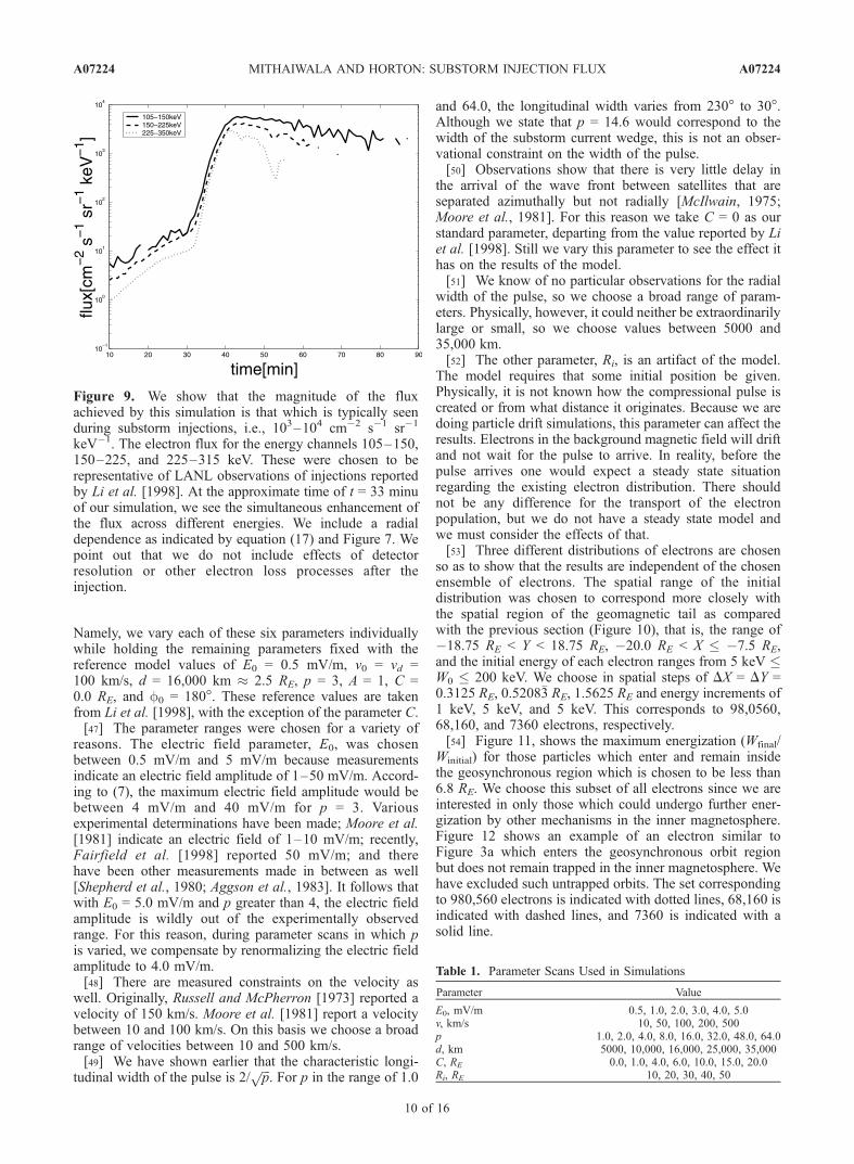
are a0 = 3, nl = 4, ml = 10, and a0d = 6. The electrons aregiven a weighting according to this function which is shownin Figure 7.[43] Figure 9 shows the electron flux for the energy

channels 105–150, 150–225, and 225–315 keV. Thesewere chosen to be representative of LANL observations ofinjections reported by Li et al. [1998]. The simultaneousflux enhancement across different energies is the key featureof dispersionless electron injections. Similar results wereobtained by Li et al. [1998]. However, in our simulation wedo not include a background flux that would normally bemeasured by a satellite in the magnetosphere but do includea radial dependence as indicated by equation (17) andFigure 7. This background is typically 102–103 cm$2 s$1

sr$1 keV$1, whereas our initial level is 100–101 cm$2 s$1

sr$1 keV$1. This initial level is due to electrons randomlydrifting into our virtual detector. We simply show that themagnitude of the flux achieved by this simulation is thatwhich is typically seen during substorm injections, i.e.,103–104 cm$2 s$1 sr$1 keV$1. We further point out thatwe do not include effects of detector resolution or otherelectron loss processes after the injection.

4.1. Results of Further Simulations and the SubstormInjection Flux

[44] Conservation of phase space density, or Liouville’stheorem, it is clear that electrons with energies less than100 keV have sufficient phase space density to account fortypical MeV electron fluxes [Kim et al., 2000; Ingraham etal., 2001]. However, it is unreasonable to assume that allthese electrons can be convected to geosynchronous orbit.Since in our simulation, an electron placed in the tail fieldwill undergo energy-dependent r?B drift out of the tail andhit the magnetopause, this occurs for a large number ofelectrons in our simulation, particularly the higher-energyelectrons.[45] In other simulations we varied the parameters and

integrated a tail distribution of electrons. The purpose of thisstudy is twofold: to determine the influence of the modelparameters on energization and transport of particles fromthe tail during substorm injections and to determine the fluxof electrons that would enter geosynchronous orbit in orderto be further energized to MeV and higher energies.[46] Orbits are computed with one-dimensional parameter

scans for the parameters listed below in the Table 1.

Figure 6. The energization (final energy divided by initialenergy) as a function of time. It is clear that those electronsgaining the most energy are coincident with the arrival ofthe dipolarization pulse at the detectors. The detectors areindicated by black squares in Figure 8.

Figure 7. The electrons are weighted according to theinitial radial distribution from equation (17).

Figure 8. The initial spatial region of electrons was 7.5 RE

/ r / 20 RE in increments of 0.1 RE, 0! . f < 360! inincrements of 1!, and energies from 1 keV / W / 512 keVin increments of 1 keV. Here we show the initial location ofelectrons that were detected by the virtual satellites that areindicated by black squares. There are seven virtual detectorsplaced at 6.6 ± 0.2 RE at local times from 2100 to 0300 LT.


9 of 16

A07224

Namely, we vary each of these six parameters individuallywhile holding the remaining parameters fixed with thereference model values of E0 = 0.5 mV/m, v0 = vd =100 km/s, d = 16,000 km , 2.5 RE, p = 3, A = 1, C =0.0 RE, and f0 = 180!. These reference values are takenfrom Li et al. [1998], with the exception of the parameter C.[47] The parameter ranges were chosen for a variety of

reasons. The electric field parameter, E0, was chosenbetween 0.5 mV/m and 5 mV/m because measurementsindicate an electric field amplitude of 1–50 mV/m. Accord-ing to (7), the maximum electric field amplitude would bebetween 4 mV/m and 40 mV/m for p = 3. Variousexperimental determinations have been made; Moore et al.[1981] indicate an electric field of 1–10 mV/m; recently,Fairfield et al. [1998] reported 50 mV/m; and therehave been other measurements made in between as well[Shepherd et al., 1980; Aggson et al., 1983]. It follows thatwith E0 = 5.0 mV/m and p greater than 4, the electric fieldamplitude is wildly out of the experimentally observedrange. For this reason, during parameter scans in which pis varied, we compensate by renormalizing the electric fieldamplitude to 4.0 mV/m.[48] There are measured constraints on the velocity as

well. Originally, Russell and McPherron [1973] reported avelocity of 150 km/s. Moore et al. [1981] report a velocitybetween 10 and 100 km/s. On this basis we choose a broadrange of velocities between 10 and 500 km/s.[49] We have shown earlier that the characteristic longi-

tudinal width of the pulse is 2/ffiffiffi

pp

. For p in the range of 1.0

and 64.0, the longitudinal width varies from 230! to 30!.Although we state that p = 14.6 would correspond to thewidth of the substorm current wedge, this is not an obser-vational constraint on the width of the pulse.[50] Observations show that there is very little delay in

the arrival of the wave front between satellites that areseparated azimuthally but not radially [McIlwain, 1975;Moore et al., 1981]. For this reason we take C = 0 as ourstandard parameter, departing from the value reported by Liet al. [1998]. Still we vary this parameter to see the effect ithas on the results of the model.[51] We know of no particular observations for the radial

width of the pulse, so we choose a broad range of param-eters. Physically, however, it could neither be extraordinarilylarge or small, so we choose values between 5000 and35,000 km.[52] The other parameter, Ri, is an artifact of the model.

The model requires that some initial position be given.Physically, it is not known how the compressional pulse iscreated or from what distance it originates. Because we aredoing particle drift simulations, this parameter can affect theresults. Electrons in the background magnetic field will driftand not wait for the pulse to arrive. In reality, before thepulse arrives one would expect a steady state situationregarding the existing electron distribution. There shouldnot be any difference for the transport of the electronpopulation, but we do not have a steady state model andwe must consider the effects of that.[53] Three different distributions of electrons are chosen

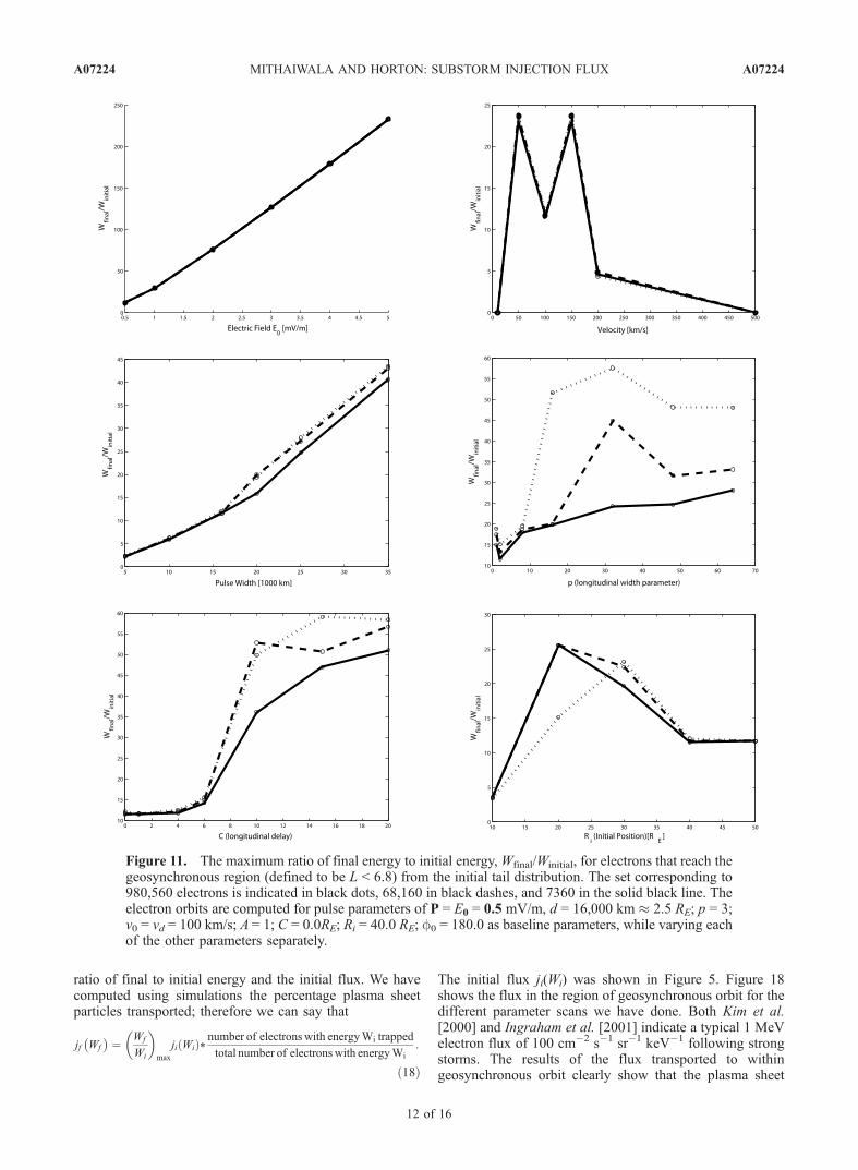
so as to show that the results are independent of the chosenensemble of electrons. The spatial range of the initialdistribution was chosen to correspond more closely withthe spatial region of the geomagnetic tail as comparedwith the previous section (Figure 10), that is, the range of$18.75 RE < Y < 18.75 RE, $20.0 RE < X . $7.5 RE,and the initial energy of each electron ranges from 5 keV .W0 . 200 keV. We choose in spatial steps of DX = DY =0.3125 RE, 0.5208!3 RE, 1.5625 RE and energy increments of1 keV, 5 keV, and 5 keV. This corresponds to 98,0560,68,160, and 7360 electrons, respectively.[54] Figure 11, shows the maximum energization (Wfinal/

Winitial) for those particles which enter and remain insidethe geosynchronous region which is chosen to be less than6.8 RE. We choose this subset of all electrons since we areinterested in only those which could undergo further ener-gization by other mechanisms in the inner magnetosphere.Figure 12 shows an example of an electron similar toFigure 3a which enters the geosynchronous orbit regionbut does not remain trapped in the inner magnetosphere. Wehave excluded such untrapped orbits. The set correspondingto 980,560 electrons is indicated with dotted lines, 68,160 isindicated with dashed lines, and 7360 is indicated with asolid line.

Figure 9. We show that the magnitude of the fluxachieved by this simulation is that which is typically seenduring substorm injections, i.e., 103–104 cm$2 s$1 sr$1

keV$1. The electron flux for the energy channels 105–150,150–225, and 225–315 keV. These were chosen to berepresentative of LANL observations of injections reportedby Li et al. [1998]. At the approximate time of t = 33 minuof our simulation, we see the simultaneous enhancement ofthe flux across different energies. We include a radialdependence as indicated by equation (17) and Figure 7. Wepoint out that we do not include effects of detectorresolution or other electron loss processes after theinjection.

Table 1. Parameter Scans Used in Simulations

Parameter Value

E0, mV/m 0.5, 1.0, 2.0, 3.0, 4.0, 5.0v, km/s 10, 50, 100, 200, 500p 1.0, 2.0, 4.0, 8.0, 16.0, 32.0, 48.0, 64.0d, km 5000, 10,000, 16,000, 25,000, 35,000C, RE 0.0, 1.0, 4.0, 6.0, 10.0, 15.0, 20.0Ri, RE 10, 20, 30, 40, 50


10 of 16

A07224

[55] We also show in Figure 13, the ratio of electrons thatreach the geosynchronous region (again defined to be L <6.8) to the initial electron population. This is an importantindicator of the effectiveness of the substorm model inconvecting tail particles earthward into the trapping area.Figure 14.[56] One must note that the percentage shown here is

dependent on what is selected as the initial distribution ofparticles, i.e., there are statistical fluctuations associatedwith the distribution we choose. Therefore what these ratiosindicate is the relative effectiveness of the parameters andnot either the number of plasma sheet particles or anabsolute percentage that can be transported to the innermagnetosphere. However, since we consider such a broadsampling of the spatial and energy distribution and simu-lations show that the results are mostly independent of thissampling, we use these results as an absolute percentage toestimate properties of the plasma sheet.[57] The implications for the varying the parameter E0 is

clear from Figures 11a and 13a. We note again that themaximum electric field strength is given by E0 ' 2p.Although increasing the electric field strength clearly ener-gizes the particles more, the maximum number of simulatedelectrons trapped is 40% at E0 = 3.0 mV/m. The energiza-tion increases from roughly 10 for E0 = 0.5 mV/m to 250 forE0 = 5.0 mV/m. This would be consistent with the singleelectron orbits of Figure 4a, which show that increasing theelectric field causes the electron to gain energy.[58] Figure 11b shows that energization with changing

velocity v0 is well correlated with the percent of electrons

convected to geosynchronous orbit. Very slow (10 km/s)and very fast (greater than 200 km/s) pulses are noteffective in transporting a high injected flux from theplasma sheet. Both the energy gain in Figure 11b andthe fraction of transported electrons in Figure 13b aremaximum at 50 km/s. This is in agreement with othermeasurements [Russell and McPherron, 1973; Moore etal., 1981]. Moore et al. [1981] postulate that the lowpropagation speed can be explained by oxygen loadingfrom the ionosphere. The single electron orbits of Figure 4bshow similar results.[59] One must take care in interpreting changes to the

longitudinal width parameter p as the maximum electricfield amplitude increases with increasing p while decreasingthe longitudinal width as in (7). As this is the case, in orderto separate the effect of the longitudinal pulse width byitself, the electric field parameter in Figures 11c and 13c istaken to be E0/2

p with E0 = 4.0 mV/m in order to makecomparisons with the other simulation in which E0 =0.5 mV/m and p = 3, giving a maximum field amplitudeof 4.0 mV/m. Figures 11c and 13c indicate that smallerlongitudinal widths or larger parameter p have largerenergization, although the total number of transportedelectrons is much smaller. It would be expected that in awider pulse the particle is under the influence of the electricfield for a longer time, so the energization there should behigher. However, we look at that portion of the populationthat gets trapped, and since it is very easy for electrons todrift out of the electric field, the electron population that istransported sees a stronger electric field on average and isenergized more when the pulse is narrow. However, the totalsize of this population is very small, as indicated inFigure 13c. The single particle orbits, shown in Figure 4c,verify that it is much easier for an electron to stay in theelectric field for a wider pulse than a narrower pulse.[60] Larger radial pulse widths also energize electrons

better due to the fact that they stay in a region of largerelectric field longer, and larger pulse widths, controlled bythe parameter d, are better at transporting larger numbers ofparticles as well. This is indicated in Figures 11d and 13d.Figure 4d would lead to a similar conclusion.[61] Figures 11e and 13e show that increasing longitudi-

nal delay parameter, C, above 6 RE dramatically increasesenergization but only moderately increases the transport ofparticles. This behavior is most easily understood by refer-ence to the single electron orbits of Figure 4f. With a largervalue of C, the electron is able to see an electric fieldat different times in its orbit (Figures 4f and 4g with C =20.0 RE) so the integrated electric field is large, rather thanonly once (Figures 4f and 4g with C = 1.0 RE).[62] The optimum initial radial position, Ri, of the pulse

according to Figures 11f and 13f is !20–30 RE. We repeatthat this parameter is a numerical artifact only; no defin-itive statements about the physical origin of the pulse inthe tail can be made. As the initial starting point of thepulse is increased, many fewer electrons are trapped. Thisis most likely because many electrons have time to rBdrift away before the pulse arrives. This is consistent withFigure 4e.[63] We can then calculate the flux transported to geo-

synchronous orbit from the tail as follows. Equation (15)tells how the flux at geosynchronous orbit is related to the

Figure 10. The spatial region for simulations of kappadistribution particles was chosen to correspond more closelywith the spatial region of the geomagnetic tail, that is, therange of $18.75 RE . Y . 18.75 RE, 7.5 RE . $X .20.0 RE in spatial steps of DX = DY = 0.3125 RE. The initialenergy of each electron ranges from 5 keV . W . 200 keV.In other simulations, spatial steps of 0.5208!3 and 1.5625were used, but are not shown here. The circle is marked at6.8 RE as reference and to indicate the trapping region.


11 of 16

A07224

ratio of final to initial energy and the initial flux. We havecomputed using simulations the percentage plasma sheetparticles transported; therefore we can say that

jf Wf

$ %

¼ Wf

Wi

& '

max

ji Wið Þ*number of electronswith energyWi trapped

total number of electronswith energyWi:

ð18Þ

The initial flux ji(Wi) was shown in Figure 5. Figure 18shows the flux in the region of geosynchronous orbit for thedifferent parameter scans we have done. Both Kim et al.[2000] and Ingraham et al. [2001] indicate a typical 1 MeVelectron flux of 100 cm$2 s$1 sr$1 keV$1 following strongstorms. The results of the flux transported to withingeosynchronous orbit clearly show that the plasma sheet

Figure 11. The maximum ratio of final energy to initial energy,Wfinal/Winitial, for electrons that reach thegeosynchronous region (defined to be L < 6.8) from the initial tail distribution. The set corresponding to980,560 electrons is indicated in black dots, 68,160 in black dashes, and 7360 in the solid black line. Theelectron orbits are computed for pulse parameters of P = E0 = 0.5 mV/m, d = 16,000 km , 2.5 RE; p = 3;v0 = vd = 100 km/s; A = 1; C = 0.0RE; Ri = 40.0 RE; f0 = 180.0 as baseline parameters, while varying eachof the other parameters separately.


12 of 16

A07224

electrons, with energies less than 200 keV, are enough toaccount for the relativistic electrons.[64] On the basis of these results, it is puzzling that

enhancement of MeV electrons is not seen during substormsand is usually seen a few days following storms. It wasproposed by Ingraham et al. [2001] that the large MeVelectron curvature and rB drift velocity removes theseelectrons rapidly from the detector region and thus are notseen. Their velocity dispersion analysis indeed shows thatMeV electrons as well as the lower-energy (<300 keV)electrons are both injected during substorm dipolarizations.Typical loss process such as scattering into the loss conecould serve to remove the electrons. We do not claim,however, that substorms themselves, in general, produceall the high-energy electrons, only that at lower energies,there is sufficient flux enhancement to provide the sourcefor the MeV electrons.

5. Conclusion

[65] The flux of relativistic electrons (E > 1 MeV) in theEarth’s outer radiation belt (3 < L < 7) varies substantiallyduring geomagnetic storms. Often the flux may fall by up toa few orders of magnitude at the beginning of the mainstorm phase and may rise to levels 10–100 times the initialvalues over the next 2–3 days during the recovery phase. It

is proposed that substorm injections can provide a seedpopulation of electrons, such that other in situ accelerationmechanisms can energize this population to relativisticenergies. Meredith et al. [2002] find that the gradualacceleration of electrons to relativistic energies duringstorms can be effective only when there are periods ofprolonged substorm activity following the main phase of thestorm. We show that substorm injections can provide asufficient flux of electrons in the inner magnetosphere sothat in situ acceleration mechanisms can be a viablemechanism for the creation of relativistic electrons afterstorms.[66] The series of simulations performed here also con-

firm the principal findings of Li et al. [1998] that electro-magnetic pulses, which are meant to model compressionalwaves of the form observed in substorms [Russell andMcPherron, 1973; Moore et al., 1981], transport electronsinto the inner magnetosphere across the geosynchronousorbit. The model used here is a nine-parameter particletracing model. The injection of these electrons is dispersion-less and the flux of these electrons coincides with what isobserved by satellites.[67] We have performed a series of simulations for

different energy intervals of the initial electron ensembleswith various initial spatial configurations of the initialelectron ensembles and scans over a wide range of theelectromagnetic model pulse parameters. The pulse param-eters that we are interested in are the electric field strength,the pulse velocity, the radial and longitudinal width, thelongitudinal velocity or equivalently longitudinal delay, andinitial pulse position.[68] Single electron orbits, as shown in Figure 4, are

instructive in gaining physical insight into what determinestransport from the tail to the inner magnetosphere. However,these must be confirmed by doing multiparticle simulations.The most important properties in determining the hardnessand intensity of the energetic electrons from the substormdipolarization pulse are the earthward propagation velocityv0, longitudinal width of the pulse controlled by the pparameter, and strength of the electric and magnetic fieldscontrolled by the E0 parameter. The strength of the electricfield is of course important as this gives the electrons itsenergy, but there is a limit to the effectiveness of convectingelectrons. Initializing the pulse somewhere around 20 RE

also seems to give the most effective energization ratherthan initializing further down the tail, but again we repeatthat this parameter is a numerical artifact of the model andnot necessarily very physical.[69] For the cases considered, we find that the flux of

electrons transported from the plasma sheet trapped in theinner magnetosphere is sufficient to account for the flux ofelectrons greater than 1 MeV seen after some storms. Theother electrons are lost to various regions includingthe dawnside and dayside magnetopause. Examples of theelectron energization factor Wfinal/Winitial are shown inFigure 11 and the corresponding fraction of the test particleensemble that reaches the inner magnetosphere is shown inFigure 13. We claim (Figure 18) that a substorm dipolariza-tion and electron injection can transport enough high-energyelectrons to account for the high fluxes seen after storms.[70] That large fluxes of high-energy electrons, i.e.,

electrons with energy greater than 1 MeV, are not seen

Figure 12. This shows an example of an electron orbitsimilar to Figure 3a which enters the geosynchronous orbitregion but does not remain trapped; we have not includedsuch orbits for this calculation since the electron does notremain within L = 6.8. We reason that such an electroncould be detected during an injection event, but would notbe energized to relativistic energies by other means. Theparameters chosen for this orbit are also similar to Figure 3a.P = E0 = 0.5 mV/m; d = 16,000 km , 2.5 RE; p = 3; v0 =100 km/s; A = 1; C = 0.4; Ri = 40.0 RE f0 = 180.0 withsimilar initial conditions R0 = 14.0 RE, f0 = 135.0!, W0 =25 keV.


13 of 16

A07224

following substorms is not explained, although Ingraham etal. [2001] do make proposals. The influence of multiplesubstorm injections on storm time high-energy electronsrequires a more comprehensive model of loss processes inthe radiation belts, although it seems likely that this is animportant factor.

[71] The simulations presented here lead to the conclu-sion that a low density of energetic, anisotropic (T? > Tk)electrons are injected into the inner magnetosphere by eachdipolarization pulse. As in previous studies, we use only 90!pitch angle electrons, and future work would require a fieldmodel such that this restriction can be lifted. However, such

Figure 13. Percentage of electrons that reach the geosynchronous region (defined to be L < 6.8). The setcorresponding to 980,560 electrons is indicated in black dots, 68,160 in black dashes, and 7360 in thesolid black line. The electron orbits are computed for pulse parameters.


14 of 16

A07224

anisotropic electron distributions drive whistler wavesunstable [Gary, 1993], and whistler waves are widelyobserved in the postmidnight to morning sector of the insidethe geosynchronous radius of the magnetosphere [Smith et

al., 1996]. Thus we suggest that an important next step inthis problem is to couple these injected flux global testparticle calculations to the local flux tube PIC simulationsand quasilinear calculations for the nonlinear evolution of

Figure 14. A comparison of the measured flux in the plasma sheet with the fluxes that can be obtainedwithin geosynchronous orbit due to substorm injection. The initial flux is indicated in blue and is thesame as Figure 5. The 1 MeV flux of electrons following a storm can be 100 cm$2 s$1 sr$1 keV$1. Theflux of plasma sheet electrons below 200 keV transported during substorms is enough to account forthe relativistic electrons. See color version of this figure at back of this issue.


15 of 16

A07224

whistlers fluctuations on the appropriate inner magneto-sphere magnetic flux tubes. Using the simulations devel-oped here as the injection source of higher-energyanisotropic electrons would be a new feature for whistlercalculations. The whistler chorus is often involved as both amechanism for scattering the electrons into the loss coneand as a mechanism for further hardening the energy of themedium-energy electrons to form the high-energy relativis-tic electrons.

[72] Acknowledgments. The authors give many thanks to TomMoore and Xinlin Li for helpful discussions. This work was supported inpart by the NSF grant ATM-0229863.[73] Lou-Chuang Lee thanks Isidoros Doxas and another reviewer for

their assistance in evaluating this paper.

ReferencesAggson, T. L., J. P. Heppner, and N. C. Maynard (1983), Observations oflarge magnetospheric electron fields during the onset phase of a sub-storm, J. Geophys. Res., 88, 3981–3990.

Arnoldy, R. L., and K. W. Chan (1969), Particle substorms observed at thegeostationary orbit, J. Geophys. Res., 74, 5019–5028.

Baker, D. N., P. R. Higbie, E. W. Hones Jr., and R. D. Belian (1978), High-resolution energetic particle measurements at 6.6 RE: 3. Low-energyelectron anisotropies and short-term substorm predictions, J. Geophys.Res., 83, 4863–4868.

Baker, D. N., J. B. Blake, L. B. Callis, R. D. Belian, and T. E. Cayton(1989), Relativistic electrons near geostationary orbit: Evidence forinternal magnetospheric acceleration, Geophys. Res. Lett., 16, 559–562.

Baker, D. N., X. Li, J. B. Blake, and S. G. Kanekal (1998), Strong electronacceleration in the earths’s magnetosphere, Adv. Space Res., 21, 609–613.

Birn, J., M. F. Thomsen, J. E. Borovsky, G. D. Reeves, D. J. McComas, andR. D. Belian (1998), Substorm electron injections: Geosynchronous ob-servations and test particle simulations, J. Geophys. Res., 103, 9235–9248.

Cayton, T. E., R. D. Belian, S. P. Gary, T. A. Fritz, and D. N. Baker (1989),Energetic electron components at geosynchronous orbit, Geophys. Res.Lett., 16, 147–150.

Christon, S. P., D. J. Williams, D. G. Mitchell, C. Y. Huang, and L. A.Frank (1991), Spectral characteristics of plasma sheet ion and electronpopulations during disturbed geomagnetic conditions, J. Geophys. Res.,96, 1–22.

Daglis, I. A., R. M. Thorne, W. Baumjohann, and S. Orsini (1999), Theterrestrial ring current: Origin, formation, and decay, Rev. Geophys., 37,407–438.

Delcourt, D. C., J. A. Sauvaud, and A. Pedersen (1990), Dynamics ofsingle-particle orbits during substorm expansion phase, J. Geophys.Res., 95, 20,853–20,865.

Fairfield, D. H., et al. (1998), Geotail observations of sustorm onset in theinner magnetotail, J. Geophys. Res., 103, 103–117.

Gary, S. P. (1993), Theory of Space Plasma Microinstabilities, CambridgeUniv. Press, New York.

Ingraham, J. C., T. E. Cayton, R. D. Belian, R. A. Christensen, R. H. W.Friedel, M. M. Meier, G. D. Reeves, and M. Tuszewski (2001), Substorminjection of relativistic electrons to geosynchronous orbit during the greatmagnetic storm of March 24, 1991, J. Geophys. Res., 106, 25,759–25,776.

Kamide, Y., et al. (1998), Current understanding of magnetic storms:Storm-substorm relationships, J. Geophys. Res., 103, 17,705–17,728.

Kim, H. J., A. A. Chan, R. A. Wolf, and J. Birn (2000), Can substormsproduce relativistic outer-belt electrons?, J. Geophys. Res., 105, 7721–7736.

Kivelson, M. G., S. M. Kaye, and D. J. Southwood (1979), The physics ofplasma injection events, in Dynamics of the Magnetosphere, p. 385,Springer, New York.

Li, X., I. Roth, M. Temerin, J. R. Wygant, M. K. Hudson, and J. B. Blake(1993), Simulation of the prompt energization and transport of radiationbelt particles during the March 24, 1991, SSC, Geophys. Res. Lett., 20,2423–2426.

Li, X., D. N. Baker, M. Temerin, D. Larson, R. P. Lin, D. Reeves, M. D.Looper, S. G. Kanekal, and R. A. Mewaldt (1997), Are energetic elec-trons in the solar wind the source of the outer radiation belt?, Geophys.Res. Lett., 24, 923–926.

Li, X., D. N. Baker, M. Temerin, G. Reeves, and R. Belian (1998), Simula-tion of dispersionless injections and drift echoes of energetic electronsassociated with substorms, Geophys. Res. Lett., 25, 3736–3766.

Littlejohn, R. (1983), Variational principles of guiding center motion,J. Plasma Phys., 29, 111–125.

Lyons, L. R., and D. J. Williams (1984), Quantitative Aspects of Magneto-spheric Physics, Springer, New York.

McIlwain, C. E. (1974), Substorm injection boundaries, in MagnetosphericPhysics, edited by B. M. McCormac, p. 143, Springer, New York.

McIlwain, C. E. (1975), Auroral electron beams near the magneticequator, in Physics of the Hot Plasma in the Magnetosphere, edited byB. Hultquist and L. Stenflo, p. 91, Plenum, New York.

McPherron, R. L. (1995), Magnetospheric dynamics, in Introduction toSpace Physics, edited by M. G. Kivelson and P. T. Russell, CambridgeUniv. Press, New York.

Meredith, N. P., R. B. Horne, R. H. A. Iles, R. M. Thorne, D. Heynderickx,and R. R. Anderson (2002), Outer zone relativistic electron accelerationassociated with substorm-enhanced whistler mode chorus, J. Geophys.Res., 107(A7), 1144, doi:10.1029/2001JA900146.

Moore, T. E., R. L. Arnoldy, J. Feynman, and D. A. Hardy (1981), Propa-gating substorm injection fronts, J. Geophys. Res., 86, 6713.

Northrop, T. G. (1963), The Adiabatic Motion of Charged Particles, Wiley-Interscience, Hoboken, N. J.

Russell, C. T., and R. L. McPherron (1973), The magnetotail and sub-storms, Space Sci. Rev., 15, 205.

Sarris, T. E., X. Li, N. Tsaggas, and N. Paschalidis (2002), Modelingenergetic particle injections in dynamic pulse fields with varying propa-gation speeds, J. Geophys. Res., 107(A3), 1033, doi:10.1029/2001JA900166.

Shepherd, G. G., R. Bostrom, H. Derblom, C.-G. Falthammar, R. Gendrin,K. Kaila, R. Pellinen, A. Korth, A. Pedersen, and G. Wrenn (1980),Plasma and field signatures of poleward propagating auroral precipitationobserved at the foot of the GEOS 2 field line, J. Geophys. Res., 85,4587–4601.

Smith, A. J., M. P. Freeman, and G. D. Reeves (1996), Postmidnight VLFchorus events, a substorm signature observed at the ground near L = 4,J. Geophys. Res., 101, 24,641–24,653.

Tsyganenko, N. A., and D. P. Stern (1996), Modeling the global magneticfield of the large-scale birkeland current systems, J. Geophys. Res., 101,27,187–27,198.

Vasyliunas, D. J. (1968), A survey of low-energy electrons in the eveningsector of the magnetosphere with OGO 1 and OGO 3, J. Geophys. Res.,73, 2839.

Zaharia, S., C. Z. Zheng, and J. R. Johnson (2000), Particle transport andenergization associated with disturbed magnetospheric events, J. Geo-phys. Res., 105, 18,471.

$$$$$$$$$$$$$$$$$$$$$$$M. Mithaiwala and W. Horton, Institute for Fusion Studies, University of

Texas at Austin, Austin, TX 78712, USA. ([email protected])


16 of 16

A07224

Figure 4. The electron orbit under different variations of the pulse parameters. The electron orbits arecomputed for pulse parameters of P = E0 = 0.5 mV/m, d = 16,000 km , 2.5 RE; p = 3; v0 = vd = 100 km/s;A = 1; C = 0.0 RE; Ri = 40.0 RE; f0 = 180.0 as baseline parameters, while varying each of the otherparameters separately.

A07224 MITHAIWALA AND HORTON: SUBSTORM INJECTION FLUX A07224

6 of 16

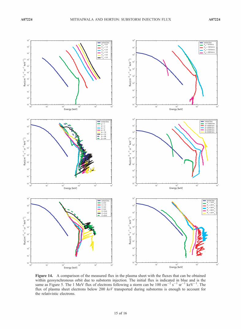
Figure 14. A comparison of the measured flux in the plasma sheet with the fluxes that can be obtainedwithin geosynchronous orbit due to substorm injection. The initial flux is indicated in blue and is thesame as Figure 5. The 1 MeV flux of electrons following a storm can be 100 cm$2 s$1 sr$1 keV$1. Theflux of plasma sheet electrons below 200 keV transported during substorms is enough to account forthe relativistic electrons.

A07224 MITHAIWALA AND HORTON: SUBSTORM INJECTION FLUX A07224

15 of 16

substorm injections pr oduce sufficient electr on

Documents