suburban nation: estimating the size of canada's...
TRANSCRIPT

Journal of Architectural and Planning Research30:3 (Autumn, 2013) 196
interests incorporate environmental behavioral studies, including residents’ perceptions of safety in gated andnon-gated communities, crime prevention through environmental design, residential designs in various cultures,green and affordable housing design and related policies, post-occupancy evaluations in various architecturalenvironments, new urbanism, and healthcare research.
You Mi Lee, PhD, is Associate Professor in the Department of Consumer and Housing Studies at SangmyungUniversity, South Korea. Her major research interests include urban housing, crime-free urban housing, andenvironmentally friendly housing.
Eunsil Lee, PhD, is Assistant Professor of Interior Design in the School of Planning, Design, and Construction atMichigan State University. Her principle areas of research address human perception and behaviors in relation toculture, including cross-cultural analysis of residential design, cross-cultural housing adjustment processes, culturaldifferences in lighting perception, and the relationship between workplace design and national culture.
Manuscript revisions completed 1 July 2013.
Copyright © 2013, Locke Science Publishing Company, Inc.Chicago, IL, USA All Rights Reserved
Journal of Architectural and Planning Research30:3 (Autumn, 2013) 197
SUBURBAN NATION? ESTIMATING THE SIZE OFCANADA’S SUBURBAN POPULATION
David L. A. GordonMark Janzen
Canada is a suburban nation. The research for this article developed new models to define andclassify suburbs and then estimated the proportion of Canadians who live in suburbs. Theresearch method extracted and classified census tract data with basic geographic informationsystem software to test definitions of suburbs for all 33 census metropolitan areas in Canada anda sample of census agglomerations. We checked anomalies using the Google Earth and GoogleStreet View mapping services, and an expert panel examined the results. Density classificationsproved most useful for classifying exurban and rural areas. The most reliable definitions of inner-city and suburban development emerged from journey-to-work data. Active cores were definedas areas with higher proportions of active transportation (walking and cycling). We tested12 models for classifying suburbs, with the most credible results emerging for a model classifyingactive cores, transit suburbs, auto suburbs, and exurban areas. These classification modelsestimate that suburban areas make up approximately 80% of Canada’s metropolitan populationand 66% of the total Canadian population.

Journal of Architectural and Planning Research30:3 (Autumn, 2013) 198
INTRODUCTION
We routinely hear that Canada is one of the most urbanized nations in the world (Artibise, 1988;The Canadian Press, 2012; MacGregor, 2009), but that does not mean most Canadians live inapartments and travel by public transit. Although it is estimated that approximately 80% of theCanadian population lives in an urban setting (Martel and Caron Malenfant, 2007), this categoryincludes downtown, inner-city, suburban, and exurban development. Our initial estimates indicatethat perhaps two-thirds of the Canadian population live in neighborhoods that most observerswould consider suburban (i.e., cars and many postwar single-family homes).
The existing urban/rural classification has genuine utility, since many demographic, environmen-tal, housing, and economic policies need to be different for rural areas. However, if “urban” simplymeans non-rural, then it is too broad a category for community planning. Suburban planningtechniques and problems, such as resource conservation and auto dependence, are significantlydifferent from those related to inner-city intensification and brownfield redevelopment.
The main objective of this paper and the research program on which it is based is to create a roughestimate of the number and proportion of suburban residents in Canada. We do not need an exactcount of suburban households for practical policy making. However, an improved estimate of theproportion and rate of growth of the Canadian suburban population may be useful, for example, forshaping an urban infrastructure program or for public-health research (Frank and Frumkin, 2004;Turcotte, 2009). A secondary objective is to establish a definition of “suburb” that would producecredible results across Canada. This paper describes the four-year struggle to establish a definitionthat would produce a dependable classification of neighborhoods in all 33 Canadian censusmetropolitan areas (CMAs), rather than the handful of case studies usually covered in researchstudies. We conclude with an estimate of the Canadian suburban population but leave the policyimplications for future comment.
CONTEXT FOR SUBURBS
The literature on how Canada became an urban nation was summarized by McCann and Smith(1991), while Stone (1967) described a precise method of measuring the urban population. The 1931Canadian census was the first in which the urban population exceeded the rural population. Thismeans Canada was likely an urban nation for only about half a century, since our preliminarycalculations indicate that many CMAs became majority suburban by the 1980s.
The pre-World War II urban areas had suburbs, of course, with pleasant neighborhoods of mainlysingle-family detached homes within walking distance of the central city in the 19th century andstreetcar suburbs in the early 20th century (McCann, 1996, 1999). Some superb historical scholar-ship by Richard Harris (Harris, 1996, 2004; Harris and Larkham, 1999) has demonstrated that therewas considerable diversity in these prewar neighborhoods, including unplanned suburbs whereworking-class citizens built their own homes.
In contrast, the scale and delivery of suburban development changed rapidly after 1945, as thefederal government encouraged mass home ownership with long-term mortgages at the same timethat automobile ownership soared. Large-scale land developers who were capable of buildingentire satellite communities emerged; Don Mills, a mixed-use neighborhood in Toronto, became aninfluential example of this (Hancock, 1994; Sewell, 1993). This new version of suburbia proved to bequite popular, and automobile-dependent neighborhoods expanded to comprise more than half ofCanada’s urban population in a remarkably short time — perhaps as early as 1981.
Journal of Architectural and Planning Research30:3 (Autumn, 2013) 199
Postwar suburban expansion was not unique to Canada, of course. The United States also saw arapid and wide-scale emergence of low-density, automobile-oriented suburban neighborhoods(Beauregard, 2006; Hayden, 2003). Some researchers have attacked the broad extent of Americansuburban expansion as urban sprawl (Burchell, et al., 2002; Duany, et al., 2000; Kunstler, 1993;Talen, 2012), while others have suggested it is a preferred lifestyle and a reflection of marketdemand (Bourne, 2001; Bruegmann, 2005; Gordon and Richardson, 1997; see also Christens, 2009).
American analysts typically use political boundaries to distinguish between pre-1946 inner citiesand more recent suburbs (Gans, 1968; Katz and Lang, 2003). However, this method is not reliable inCanada, where local-government annexations and amalgamations are more common (Parr, 2007;Walks, 2007). For example, cities such as Calgary and Winnipeg comprise a large proportion oftheir CMA’s population, including all inner-city and most suburban areas. Some cities, such asOttawa, also include substantial exurban and rural areas following recent local-government re-structuring.
In addition, the classification of metropolitan areas into inner-city, suburban, and rural areas masksthe growing polycentricity of North American cities (Bunting, et al., 2002; Filion, et al., 2004; Yang,et al., 2012). This polycentricity has been strongly encouraged throughout many metropolitanareas by recent planning policies that attempt to cluster development around higher-access nodesin the transit system using mobility hubs and transit-oriented development.
There is a large amount of literature on the geography of the suburban expansion of Canadiancities (Bourne and Ley, 1993; Bunting and Filion, 1999; Bunting, et al., 2002; Filion and Bunting,2006; Filion and Hammond, 2003; Millward, 2008; Smith, 2006) and a growing literature on planningCanadian suburbs (Filion, 2001; Filion and McSpurren, 2007; Friedman, 2002; Grant, 1999, 2006a,2006b, 2007; Grant, et al., 2004). Unfortunately, scholars of the history, geography, and planning ofCanadian suburbs do not appear to have produced an estimate of the extent of this phenomenonsimilar to our estimates of urban and rural populations.
However, two Canadian researchers have recently considered how the downtown/suburban/ruralspectrum might be analyzed. Alan Walks (2004, 2005) classified inner-city, inner-suburban, andouter-suburban neighborhoods to inform his political analysis of Canadian metropolitan areas. Heused the edge of the built-up area in 1945 and 1970 as the boundary between the inner city and theinner suburbs. Walks (2007) concluded that his classification based on urban form outperformed aclassification based on local-government boundaries for explaining variations in political supportfor post-war federal elections in the three largest metropolitan regions in Canada.
Statistics Canada analyst Martin Turcotte (2008b) reviewed four criteria for distinguishing be-tween urban and suburban neighborhoods: political boundaries, zones outside the inner city,distance from the city center, and neighborhood density. He dismissed political boundaries asbeing unreliable given the variation in local-government structures across the nation. The zonesoutside the inner city were similar to Walks’s inner-city/inner-suburb/outer-suburb classification,but Turcotte found too many difficulties in establishing rules for classifying the zones. Similarly,distance from the city center was not a good criterion for comparing the structure of large and smallmetropolitan areas since a 5 km (3.1 mi) radius might incorporate the inner city in a large metropolisand the entire urban area of a smaller city. Turcotte found neighborhood density to be the leastobjectionable method for distinguishing between urban and suburban areas. He used the propor-tion of single-family detached and semidetached houses as a proxy for density to remove some ofthe problems with calculating gross population density that are created by employment areas,water bodies, rural areas, and airports. The low-density areas were defined as census tracts (CTs),consisting of more than 66% single-family detached and semidetached housing units. These low-density areas contained more than 50% of the population of the metropolitan areas (ibid.:7).

Journal of Architectural and Planning Research30:3 (Autumn, 2013) 200
RESEARCH METHODS
Overview of Data Sources and Methods
The primary research method used for this paper was the classification of the 2006 and 1996Canadian censuses for all 33 CMAs. The classification was based entirely on secondary data; themain source was Statistics Canada (2001, 2006) summary data at the CT level. The Canadian censusis the obvious source of data for this research because it collects data on housing types (McCall,2009), population characteristics, and travel to work and summarizes the results at a variety ofscales (Mendelson, 2001). The 2006 census marked the end of several decades of consistent datacollection in this series due to 2011 changes that made the “long form” questionnaire optional.
We used aerial and ground photography distributed online by the Google Earth and Google StreetView mapping services to check the data classification and analysis for anomalies. The age of theGoogle Earth aerial photography varied for different municipalities, but the Canadian Google StreetView images were mostly taken in 2009, three years after the last census data were collected.
We carried out the classification and analysis of the CTs with simple descriptive statistics usingspreadsheets. We transformed the results into choropleth maps using ArcMap geographic infor-mation system (GIS) software and then exported them in .kml format to the Google Earth mappingservice for error checking. We used the Google Earth and Google Street View mapping services toreview apparent anomalies and the morphology of neighborhoods that straddled the divides in theclassifications. The morphology of road networks and building types was readily visible usingthese two resources.
We also used personal knowledge during the review process, producing models and maps for thehome cities of the peer reviewers, research assistants, and principal investigators. In this manner,we obtained informed reviews of over half the CMAs. The Google Earth and Google Street Viewmapping services were particularly useful for this review process, especially in the cities aboutwhich the team had less personal knowledge. The reliability of the review process was strength-ened by training the research assistants using familiar cities before comparing the classifications inothers. Knowledgeable local academics and municipal planners were contacted to resolve finalanomalies in a few cases.
Creating Working Definitions
A principal difficulty in estimating the extent of suburban development is defining the phenome-non. There is currently no standard definition, and it is unlikely that a single definition would fit allof the policy analysis requirements. However, there is no reason why working definition(s) couldnot be developed to help consider the policy implications of suburbia. Our objective was toproduce “roughly correct” definitions for practical policy making, similar to Statistics Canada’s setof six definitions of “rural” (du Plessis, et al., 2001, 2002).
Previous research (Galster, et al., 2001; Mendelson, 2001; Talen, 2003; Torrens, 2008) has indicatedthat measuring urbanization requires careful attention to methodological issues, even for relativelysimple calculations like the ones proposed for this project. Some interesting approaches to themeasurement of suburbs have emerged recently (Bagley, et al., 2002; Forsyth, 2012; Parr, 2007;Song and Knapp, 2007), but they deal mostly with survey data collected for specific areas, ratherthan census information that could be used across a diverse country, such as Canada. StatisticsCanada developed a variety of techniques for estimating the size of the rural population usingcensus data, recommending that policy analysts use the definition that most closely fits theproblem they are addressing (du Plessis, et al., 2001, 2002).
Journal of Architectural and Planning Research30:3 (Autumn, 2013) 201
Some initial methodological considerations were extracted from the literature. Using politicalboundaries of urban and suburban municipalities did not look promising due to varying municipalgovernance structures and annexations (Parr, 2007). Instead, the CT program is the ideal level ofanalysis for urban-planning purposes at the neighborhood level (Leung, 2003:Ch. 4). The 1951start for CTs fits the postwar era’s rapid expansion of suburban development (Harris, 2004; Hodgeand Gordon, 2013:Ch. 5) and allows for time-series analysis of some variables. Although there maybe small variations within CTs, the boundaries have been carefully selected to fit relatively homo-geneous neighborhoods, with an average population of about 5,000. The CT boundaries are alsostable — they may split after growth, but they rarely change, making time-series analysis mucheasier (Mendelson, 2001).
Although classifying suburban neighborhoods has its difficulties, other imprecise conceptssuch as “urban,” “inner city,” and “downtown” have been measured and compared for years, asdiscussed above. Ley and Frost’s (2006) definition of inner city provides several lessons. It isbased on a comparison of the proportion of pre-1946 dwellings in a CT to the proportion of pre-1946 dwellings in the entire CMA.1 In their study, if an individual CT had a larger proportion ofolder buildings than the CMA average, it was classified as inner city. This definition producedcredible results for both large and small CMAs because it did not try to force one threshold acrosscities of all sizes. Similarly, it produced good results in most parts of Canada because it used thelocal proportion of older buildings as the criterion. Many older eastern cities have a larger propor-tion of pre-1946 housing stock. Finally, the local proportion of older buildings dropped with eachcensus, as more new housing was built. Since the classification was based on the proportion ofolder housing, the inner city was allowed to expand over time, and some older streetcar suburbslike Ottawa’s Westboro were added to the inner-city classification in a manner that seemedcredible.
Density and built-form variables have been used in many studies. Researchers have found grossdensity and distance from the city center to be important variables in suburban transportationanalysis (Boarnet and Crane, 2001; Ewing and Cervero, 2001, 2010; Filion, et al., 2006; Levinson andKumar, 1997; Muller, 2004). However, gross population density is difficult to measure in a compa-rable manner due to the presence of employment areas, water bodies, and environmental protec-tion areas (Gordon and Vipond, 2005). It is not entirely clear why density has performed so well inthese analyses, but it appears to be representing a composite of urban-form variables. Otheranalysts have attempted to classify neighborhoods more directly using urban morphology con-cepts, such as street connectivity, intersection density, and building types, converted for measure-ment in GIS systems (Song and Knapp, 2007). However, meta-analyses have indicated that urbandesign variables have little correlation to vehicular travel for the journey to work (Crane, 2000;Ewing and Cervero, 2001, 2010).
Starting from these previous attempts to define the inner city and suburbs, the research team forthis project developed simple models to classify and map definitions of suburbs at the CT levelusing spreadsheets and GIS. The first step was a pilot study that tested many of these variables forthe Ottawa-Gatineau CMA, as described below. The study team then tested several promisingdefinitions of suburbs in 10 CMAs. Next, we used expert judgment to refine and adjust severalworking definitions of suburbs. A panel of six expert geography and planning researchers dis-cussed the definitions and suggested ways to improve alternative definitions applied in six CMAsduring an intensive workshop in a GIS laboratory.
After three potential definitions were identified, the study team used them to classify most of theCMAs. CT data were extracted and sorted to calculate the size of the suburban population and itsgrowth rate from 1996-2006 for all 33 CMAs using the two most reliable families of models. Unfor-tunately, CT data were not available for many census areas (CAs) (communities with populationsover 10,000 and less than 100,000). We tested the most reliable model on a sample of the larger CAsto allow some inferences about the extent of suburban development in the towns and smaller cities.
Journal of Architectural and Planning Research30:3 (Autumn, 2013) 202
Pilot Study Results from the Ottawa-Gatineau CMA
A pilot study of this technique was completed using the Ottawa-Gatineau CMA (Gordon andVandyk, 2010). Ottawa was a particularly useful site because it has a continuous greenbelt about5 km (3.1 mi) from the city center. All of the development outside the greenbelt dates from after 1960,and most of it would be considered suburban. We mapped the expansion of the suburban neigh-borhoods from 1951-2006 using several classification schemes and an iterative process to deter-mine the schemes’ effectiveness in identifying suburban development. We used aerial photointerpretation of typical 2006 suburban characteristics to identify anomalies and compare thevarious classification schemes.
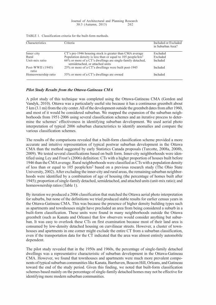
The results of the comparisons revealed that a built-form classification scheme provided a moreaccurate and intuitive representation of typical postwar suburban development in the OttawaCMA than the method suggested by early Statistics Canada proposals (Turcotte, 2008a, 2008b,2009). We tested several classifications based on built form. Inner-city neighborhoods were iden-tified using Ley and Frost’s (2006) definition: CTs with a higher proportion of houses built before1946 than the CMA average. Rural neighborhoods were classified as CTs with a population densityof less than or equal to 105 people/km2 based on a previous research study (The Ohio StateUniversity, 2002). After excluding the inner-city and rural areas, the remaining suburban neighbor-hoods were identified by a combination of age of housing (the percentage of homes built after1945); proportion of single-family detached, semidetached, and attached units (unit-mix ratio); andhomeownership ratios (Table 1).
By iteration we produced a 2006 classification that matched the Ottawa aerial photo interpretationfor suburbs, but none of the definitions we tried produced stable results for earlier census years inthe Ottawa-Gatineau CMA. This was because the presence of higher density building types suchas apartments and townhouses might have precluded an area from being considered a suburb in abuilt-form classification. These units were found in many neighborhoods outside the Ottawagreenbelt (such as Kanata and Orleans) that few observers would consider anything but subur-ban. It was easy to overlook these CTs on first examination because most of their land area isconsumed by low-density detached housing on curvilinear streets. However, a cluster of town-houses and apartments in one corner might exclude the entire CT from a suburban classification,even if the transportation data for the CT indicated that the area was almost entirely automobiledependent.
The pilot study revealed that in the 1950s and 1960s, the percentage of single-family detacheddwellings was a representative characteristic of suburban development in the Ottawa-GatineauCMA. However, we found that townhouses and apartments were much more prevalent compo-nents of typical suburban communities like Kanata, Barrhaven, Beacon Hill, Orleans, and Gatineautoward the end of the study period. Given this finding, we noted that built-form classificationschemes based mainly on the percentage of single-family detached homes may not be effective foridentifying more modern suburban communities.
TABLE 1. Classification criteria for the built-form methods._______________________________________________________________________________________________________________________________________________________________________________________________________________________________________________________________________________________________________________________________________________________________Characteristics Criteria Included or Excluded
in Suburban Area?_______________________________________________________________________________________________________________________________________________________________________________________________________________________________________________________________________________________________________________________________________________________________Inner city CT’s pre-1946 housing stock is greater than CMA average ExcludedRural Population density is less than or equal to 105 people/km2 ExcludedUnit-mix ratio 66% or more of a CT’s dwellings are single-family detached, Included
semidetached, or attached unitsPost-WWII (1945) 25% or more of a CT’s dwellings were built post-1945 Included ratioHomeownership ratio 55% or more of a CT’s dwellings are owned Included_______________________________________________________________________________________________________________________________________________________________________________________________________________________________________________________________________________________________________________________________________________________________
Journal of Architectural and Planning Research30:3 (Autumn, 2013) 203
The pilot study demonstrated one good feature of Ley and Frost’s (2006) definition of the innercity. By defining the inner city as CTs that have a higher proportion of pre-1946 dwellings than theCMA average, a slow, progressive expansion of the inner city was revealed, producing a crediblechronology of inner-city growth during the study period. This exclusion of inner-city areas provedto be an essential and robust component of future suburban classification schemes.
Another essential component of the built-form classification scheme was the exclusion of rural CTswithin the CMA. Many of the larger CTs located on the periphery of CMAs exhibited characteris-tics similar to rural areas. A population density criterion produced consistent results throughoutthe different census years and was brought forward for classifying the rural/suburban fringe insubsequent models.
Weak Results When Built-Form Methods Applied Nationally
We tested the built-form definitions proposed by Statistics Canada (Turcotte, 2008a, 2008b, 2009)and our pilot study in 10 CMAs using 2006 data. Unfortunately, built-form definitions that pro-duced reasonable results in our pilot site of Ottawa-Gatineau often produced suburban classifica-tions that made little sense in other cities. In contrast, a rural classification based on populationdensity seemed to work reasonably well in most CMAs, although there were many anomaliesassociated with oversized CTs, water bodies, and small residential developments. Water bodieswere excluded from the area of all CT maps, but large parks and new residential development on therural fringe that had not been given their own CT required that we carefully examine the associatedaerial photography by projecting the classification maps into the Google Earth mapping service.Although the density method had some difficulties when it was used for defining a rural or anexurban area, it was a more effective classification method than establishing a limit based on thedistance from the center of the CMA. A radius that was appropriate for a large CMA, such as 5 km(3.1 mi) (ibid.), would not work for a smaller CMA or the CAs.
Ley and Frost’s (2006) inner-city definition based on the proportion of pre-1946 dwellings pro-duced credible results for most smaller metropolitan areas. However, the definition began to breakdown after 1996 for the larger CMAs that were experiencing large-scale inner-city redevelopmentof their waterfronts, railway yards, and brownfields. Some Vancouver, Toronto, and Montrealdowntown CTs were not classified as inner city because they were composed entirely of newbuildings, and other central neighborhoods began to drop out of the inner-city category becausethey experienced substantial infill of new apartment buildings. As the redevelopment and infill ofinner cities continues, this flaw will become a more serious drawback to this method.
However, the most serious disadvantage of built-form definitions was the wide variation in build-ing types deployed across Canadian metropolitan areas. A lower proportion of single-family de-tached homes did not work as an exclusion criterion because of the pockets of suburban town-houses and apartments that were identified in Ottawa-Gatineau and found in almost every Canadi-an city. This phenomenon is not an accident. Standard land-use planning procedures have calledfor a mix of dwelling-unit types in suburban communities since the 1960s (Hodge and Gordon,2013; Leung, 2003). For example, Don Mills, the iconic suburb built in the 1950s, contains manyapartment buildings in the core of the community and clusters of townhouses in most neighbor-hood units (Sewell, 1993).
Similarly, the presence or absence of apartments may not signal an inner-city CT. Several of Mon-treal and Québec’s inner-city neighborhoods contain few apartments but have large concentra-tions of townhouses and stacked townhouses. These building-type anomalies confounded all ofthe classification schemes we attempted to deploy across Canada. Local and regional variations inbuilding types and densities broke all of our attempts at a standard definition. Another problemwith the built-form methods was the almost purely empirical and iterative nature of the models. Inour attempts to produce a classification model that would reproduce the results on the ground, we

Journal of Architectural and Planning Research30:3 (Autumn, 2013) 202
Pilot Study Results from the Ottawa-Gatineau CMA
A pilot study of this technique was completed using the Ottawa-Gatineau CMA (Gordon andVandyk, 2010). Ottawa was a particularly useful site because it has a continuous greenbelt about5 km (3.1 mi) from the city center. All of the development outside the greenbelt dates from after 1960,and most of it would be considered suburban. We mapped the expansion of the suburban neigh-borhoods from 1951-2006 using several classification schemes and an iterative process to deter-mine the schemes’ effectiveness in identifying suburban development. We used aerial photointerpretation of typical 2006 suburban characteristics to identify anomalies and compare thevarious classification schemes.
The results of the comparisons revealed that a built-form classification scheme provided a moreaccurate and intuitive representation of typical postwar suburban development in the OttawaCMA than the method suggested by early Statistics Canada proposals (Turcotte, 2008a, 2008b,2009). We tested several classifications based on built form. Inner-city neighborhoods were iden-tified using Ley and Frost’s (2006) definition: CTs with a higher proportion of houses built before1946 than the CMA average. Rural neighborhoods were classified as CTs with a population densityof less than or equal to 105 people/km2 based on a previous research study (The Ohio StateUniversity, 2002). After excluding the inner-city and rural areas, the remaining suburban neighbor-hoods were identified by a combination of age of housing (the percentage of homes built after1945); proportion of single-family detached, semidetached, and attached units (unit-mix ratio); andhomeownership ratios (Table 1).
By iteration we produced a 2006 classification that matched the Ottawa aerial photo interpretationfor suburbs, but none of the definitions we tried produced stable results for earlier census years inthe Ottawa-Gatineau CMA. This was because the presence of higher density building types suchas apartments and townhouses might have precluded an area from being considered a suburb in abuilt-form classification. These units were found in many neighborhoods outside the Ottawagreenbelt (such as Kanata and Orleans) that few observers would consider anything but subur-ban. It was easy to overlook these CTs on first examination because most of their land area isconsumed by low-density detached housing on curvilinear streets. However, a cluster of town-houses and apartments in one corner might exclude the entire CT from a suburban classification,even if the transportation data for the CT indicated that the area was almost entirely automobiledependent.
The pilot study revealed that in the 1950s and 1960s, the percentage of single-family detacheddwellings was a representative characteristic of suburban development in the Ottawa-GatineauCMA. However, we found that townhouses and apartments were much more prevalent compo-nents of typical suburban communities like Kanata, Barrhaven, Beacon Hill, Orleans, and Gatineautoward the end of the study period. Given this finding, we noted that built-form classificationschemes based mainly on the percentage of single-family detached homes may not be effective foridentifying more modern suburban communities.
TABLE 1. Classification criteria for the built-form methods._______________________________________________________________________________________________________________________________________________________________________________________________________________________________________________________________________________________________________________________________________________________________Characteristics Criteria Included or Excluded
in Suburban Area?_______________________________________________________________________________________________________________________________________________________________________________________________________________________________________________________________________________________________________________________________________________________________Inner city CT’s pre-1946 housing stock is greater than CMA average ExcludedRural Population density is less than or equal to 105 people/km2 ExcludedUnit-mix ratio 66% or more of a CT’s dwellings are single-family detached, Included
semidetached, or attached unitsPost-WWII (1945) 25% or more of a CT’s dwellings were built post-1945 Included ratioHomeownership ratio 55% or more of a CT’s dwellings are owned Included_______________________________________________________________________________________________________________________________________________________________________________________________________________________________________________________________________________________________________________________________________________________________
Journal of Architectural and Planning Research30:3 (Autumn, 2013) 203
The pilot study demonstrated one good feature of Ley and Frost’s (2006) definition of the innercity. By defining the inner city as CTs that have a higher proportion of pre-1946 dwellings than theCMA average, a slow, progressive expansion of the inner city was revealed, producing a crediblechronology of inner-city growth during the study period. This exclusion of inner-city areas provedto be an essential and robust component of future suburban classification schemes.
Another essential component of the built-form classification scheme was the exclusion of rural CTswithin the CMA. Many of the larger CTs located on the periphery of CMAs exhibited characteris-tics similar to rural areas. A population density criterion produced consistent results throughoutthe different census years and was brought forward for classifying the rural/suburban fringe insubsequent models.
Weak Results When Built-Form Methods Applied Nationally
We tested the built-form definitions proposed by Statistics Canada (Turcotte, 2008a, 2008b, 2009)and our pilot study in 10 CMAs using 2006 data. Unfortunately, built-form definitions that pro-duced reasonable results in our pilot site of Ottawa-Gatineau often produced suburban classifica-tions that made little sense in other cities. In contrast, a rural classification based on populationdensity seemed to work reasonably well in most CMAs, although there were many anomaliesassociated with oversized CTs, water bodies, and small residential developments. Water bodieswere excluded from the area of all CT maps, but large parks and new residential development on therural fringe that had not been given their own CT required that we carefully examine the associatedaerial photography by projecting the classification maps into the Google Earth mapping service.Although the density method had some difficulties when it was used for defining a rural or anexurban area, it was a more effective classification method than establishing a limit based on thedistance from the center of the CMA. A radius that was appropriate for a large CMA, such as 5 km(3.1 mi) (ibid.), would not work for a smaller CMA or the CAs.
Ley and Frost’s (2006) inner-city definition based on the proportion of pre-1946 dwellings pro-duced credible results for most smaller metropolitan areas. However, the definition began to breakdown after 1996 for the larger CMAs that were experiencing large-scale inner-city redevelopmentof their waterfronts, railway yards, and brownfields. Some Vancouver, Toronto, and Montrealdowntown CTs were not classified as inner city because they were composed entirely of newbuildings, and other central neighborhoods began to drop out of the inner-city category becausethey experienced substantial infill of new apartment buildings. As the redevelopment and infill ofinner cities continues, this flaw will become a more serious drawback to this method.
However, the most serious disadvantage of built-form definitions was the wide variation in build-ing types deployed across Canadian metropolitan areas. A lower proportion of single-family de-tached homes did not work as an exclusion criterion because of the pockets of suburban town-houses and apartments that were identified in Ottawa-Gatineau and found in almost every Canadi-an city. This phenomenon is not an accident. Standard land-use planning procedures have calledfor a mix of dwelling-unit types in suburban communities since the 1960s (Hodge and Gordon,2013; Leung, 2003). For example, Don Mills, the iconic suburb built in the 1950s, contains manyapartment buildings in the core of the community and clusters of townhouses in most neighbor-hood units (Sewell, 1993).
Similarly, the presence or absence of apartments may not signal an inner-city CT. Several of Mon-treal and Québec’s inner-city neighborhoods contain few apartments but have large concentra-tions of townhouses and stacked townhouses. These building-type anomalies confounded all ofthe classification schemes we attempted to deploy across Canada. Local and regional variations inbuilding types and densities broke all of our attempts at a standard definition. Another problemwith the built-form methods was the almost purely empirical and iterative nature of the models. Inour attempts to produce a classification model that would reproduce the results on the ground, we

Journal of Architectural and Planning Research30:3 (Autumn, 2013) 204
drifted further and further from the slender theoretical bases of the built-form literature. After18 months of experimentation with built-form methods, the research team switched to modelsbased on transportation methods, which immediately produced more credible results.
More Credible Results with Transportation Methods
In its long-form census, Statistics Canada collects valuable information on the mode of transporta-tion people use to get to work (Heisz and Larochelle-Côté, 2005; Martel and Caron Malenfant, 2007;Turcotte, 2008a). These data were quite useful for classifying neighborhoods according to thetransportation behavior of their residents.
Active coresOnly 7.1% of the Canadian labor force uses active transportation (walking or cycling) to get towork (Turcotte and Ruel, 2008). However, we discovered that active transportation was heavilyconcentrated in the cores of the metropolitan areas and was the dominant transportation mode insome inner-city CTs. Active transportation was a better criterion for defining the core of a city thantransit use, which should not be a surprise, since one of the principal advantages of downtownliving is the ability to walk or cycle to a job in the central business district. Transit use was highestin the inner suburbs with good transit service. These neighborhoods were too far removed fromemployment concentrations to walk or cycle to work, but a transit pass provided a convenientalternative to commuting by automobile in congested areas (see Figure 1).
We defined an “active core” as a neighborhood that has a 50% higher rate of active transportation(walking or cycling) than the overall average for the CMA. These CTs are generally in central areasand the downtowns of cities. They also include the new infill neighborhoods not classified by Leyand Frost’s inner-city definition based on pre-1946 buildings. Our definition was structured usinglocal proportions of active transportation, which had the virtue of producing results that seemedcredible across Canada in both large and small centers (Figures 2-4).2 We also tried many combina-tions of active transportation with other variables such as the ratios of households without chil-dren or pre-1946 buildings, but these additional variables did not demonstrate more credible resultsand detracted from the simplicity of the model.
In some larger cities, active cores have begun to form in some secondary centers outside of thedowntown, such as Burnaby’s MetroTown and Langley within the Vancouver CMA (see Figure 3).In larger metropolitan areas, multiple active cores were also observed in the downtowns of oldercommunities that have been absorbed into larger CMAs, such as St. Jerome in Montreal; Oakvillein Toronto; and the CMA containing the cities of Kitchener, Waterloo, and Cambridge. This is onereason for using the name “active core” as opposed to “inner city.” Based on our analysis, in 2006,approximately 2.6 million Canadians were living in active cores, making up about 12% of thepopulation in metropolitan areas (see Table 2).
Exurban areasWe defined “exurban” areas as CTs that have low gross population density and mostly depend onautomobile use. We prefer the term “exurban” to “rural” for these neighborhoods because theedges of CMAs are defined by the areas where over half of the labor force commutes to the centralcity for employment. Most of the people in these outer CTs are not engaged in rural or agrarianactivities on a full-time basis (Bollman, 2007). Although exurban areas may not be entirely includedin the suburban category, most residents live in single-family detached homes and commute byautomobile to the central city.
We tested three different definitions of “low density” for rural/exurban areas and settled on theOrganization of Economic Co-operation and Development’s “rural communities” definition, whichis limited to areas that have less than or equal to 150 people/km2. This is one of the methodsrecommended by Statistics Canada for rural lands analysis (du Plessis, et al., 2001).
Journal of Architectural and Planning Research30:3 (Autumn, 2013) 205
FIGU
RE 1. Toronto: dom
inant modes for traveling to w
ork.
Figure 1

Journal of Architectural and Planning Research30:3 (Autumn, 2013) 206
FIGU
RE 2. Toronto: transportation m
odel T8.
Journal of Architectural and Planning Research30:3 (Autumn, 2013) 207
FIGU
RE 3. Vancouver: transportation m
odel T8.
Figure 2

Journal of Architectural and Planning Research30:3 (Autumn, 2013) 206
FIGU
RE 2. Toronto: transportation m
odel T8.
Journal of Architectural and Planning Research30:3 (Autumn, 2013) 207
FIGU
RE 3. Vancouver: transportation m
odel T8.
Figure 3

Journal of Architectural and Planning Research30:3 (Autumn, 2013) 208
FIGU
RE 4. M
ontreal: transportation model T8.
Journal of Architectural and Planning Research30:3 (Autumn, 2013) 209
TABLE 2. A
ctive core, suburb, and exurban proportions in Canadian CMA
s based on the 1996 and 2006 censuses using transportation model T8 (data source: Statistics Canada, 1996, 2006).
_______________________________________________________________________________________________________________________________________________________________________________________________________________________________________________________________________________________________________________________________________________________________C
ityPop. in
Pop. inPop.
Active Core
Suburbs Exurban
19962006
growth
Pop. in%
Pop. in%
Gr.
Pop. in%
Pop. in%
Gr.
Pop. in%
Pop. in%
Gr.
19962006
19962006
19962006
_______________________________________________________________________________________________________________________________________________________________________________________________________________________________________________________________________________________________________________________________________________________________Toronto
4,262,0455,111,310
19.9%359,010
8%530,285
10%48%
3,748,98088%
4,410,42586%
18%154,055
4%170,600
3%11%
Montreal
3,326,4103,634,115
9.3%334,615
10%384,275
11%15%
2,842,36585%
3,119,09086%
10%149,430
4%130,750
4%-13%
Vancouver1,831,675
2,116,62015.6%
259,63514%
346,27516%
33%1,502,225
82%1,710,300
81%14%
69,8154%
60,0453%
-14%O
ttawa
1,010,5001,129,780
11.8%127,775
13%143,155
13%12%
733,32073%
838,79574%
14%149,405
15%147,830
13%-1%
Calgary821,595
1,079,31531.4%
123,17515%
152,69014%
24%659,495
80%874,445
81%33%
38,9255%
52,1805%
34%Edm
onton862,565
1,034,69020.0%
96,08011%
122,90512%
28%646,945
75%787,460
76%22%
119,54014%
124,32512%
4%Q
uébec671,905
712,5706.1%
96,63014%
114,87016%
19%499,885
74%512,535
72%3%
75,39011%
85,16512%
13%W
innipeg667,220
694,8504.1%
78,80012%
86,22012%
9%540,350
81%552,860
80%2%
48,0707%
55,7708%
16%H
amilton
624,320693,185
11.0%89,165
14%79,670
11%-11%
485,67578%
561,69581%
16%49,480
8%51,820
7%5%
London398,615
457,77514.8%
56,70514%
66,60515%
17%293,970
74%323,375
71%10%
47,94012%
67,79515%
41%K
itchener382,960
449,99017.5%
56,35015%
49,05011%
-13%302,625
79%376,885
84%25%
23,9856%
24,0555%
0%St. Catha-
372,415390,600
4.9%51,925
14%59,385
15%14%
266,03571%
275,58571%
4%54,455
15%55,630
14%2%
rinesH
alifax332,545
372,76512.1%
43,66513%
51,48514%
18%218,345
66%231,845
62%6%
70,53521%
89,43524%
27%O
shawa
268,755330,695
23.0%13,580
5%12,870
4%-5%
232,03086%
286,82587%
24%23,145
9%31,000
9%34%
Victoria304,330
329,9958.4%
58,56019%
59,30018%
1%224,395
74%257,185
78%15%
21,3757%
13,5104%
-37%W
indsor278,690
323,46016.1%
29,93011%
49,85515%
67%215,580
77%234,835
73%9%
33,18012%
38,77012%
17%Saskatoon
219,045233,820
6.7%25,850
12%31,285
13%21%
167,74077%
170,91573%
2%25,455
12%31,620
14%24%
Regina
193,640195,010
.7%21,725
11%31,720
16%46%
153,24079%
145,92575%
-5%18,675
10%17,365
9%-7%
Sherbrooke147,390
186,89026.8%
20,15514%
19,82511%
-2%97,570
66%129,165
69%32%
29,66520%
37,90020%
28%St. Johns
174,045181,025
4.0%25,010
14%22,815
13%-9%
123,70571%
129,32571%
5%25,330
15%28,885
16%14%
Barrie118,700
177,02049.1%
13,62011%
15,9259%
17%80,295
68%133,470
75%66%
24,78521%
27,62516%
11%K
elowna
136,535162,265
18.8%20,655
15%28,175
17%36%
85,50063%
108,79067%
27%30,380
22%25,300
16%-17%
Abbotsford
136,475158,875
16.4%4,825
4%0
0%n/a
104,92577%
135,45085%
29%26,725
20%23,425
15%-12%
Sudbury160,490
158,240-1.4%
23,96015%
23,64515%
-1%101,020
63%100,080
63%-1%
35,51022%
34,51522%
-3%K
ingston143,430
152,3306.2%
25,91018%
22,33515%
-14%78,855
55%92,880
61%18%
38,66527%
37,11524%
-4%Saguenay
160,460151,655
-5.5%13,905
9%13,580
9%-2%
95,09559%
86,56557%
-9%51,460
32%51,510
34%0%
Trois-139,940
141,3951.0%
15,05511%
18,34513%
22%95,815
68%88,940
63%-7%
29,07021%
34,11024%
17% RivièresG
uelph105,410
126,97520.5%
15,81515%
23,06018%
46%77,885
74%91,860
72%18%
11,71011%
12,0559%
3%M
oncton113,490
126,40511.4%
14,37013%
18,06514%
26%69,200
61%76,615
61%11%
29,92026%
31,72525%
6%Brantford
100,250124,745
24.4%11,420
11%11,490
9%1%
81,73082%
88,97071%
9%7,100
7%24,285
19%242%
Thunder Bay125,565
122,820-2.2%
22,96018%
13,79011%
-40%73,200
58%76,160
62%4%
29,40523%
32,87027%
12%Saint John
125,700122,280
-2.7%15,590
12%12,650
10%-19%
69,23055%
67,74555%
-2%40,880
33%41,885
34%2%
Peterbor-100,185
116,59516.4%
18,33018%
23,27520%
27%51,195
51%51,640
44%1%
30,66031%
41,68036%
36% oughTO
TAL
18,817,29521,500,060
14.3%2,184,755
12%2,638,875
12%21%
15,018,42080%
17,128,63580%
14%1,614,120
9%1,732,550
8%7%
_______________________________________________________________________________________________________________________________________________________________________________________________________________________________________________________________________________________________________________________________________________________________N
ote. Percentages may not add up to 100 due to rounding.
_______________________________________________________________________________________________________________________________________________________________________________________________________________________________________________________________________________________________________________________________________________________________
Figure 4

Journal of Architectural and Planning Research30:3 (Autumn, 2013) 208
FIGU
RE 4. M
ontreal: transportation model T8.
Journal of Architectural and Planning Research30:3 (Autumn, 2013) 209
TABLE 2. A
ctive core, suburb, and exurban proportions in Canadian CMA
s based on the 1996 and 2006 censuses using transportation model T8 (data source: Statistics Canada, 1996, 2006).
_______________________________________________________________________________________________________________________________________________________________________________________________________________________________________________________________________________________________________________________________________________________________C
ityPop. in
Pop. inPop.
Active Core
Suburbs Exurban
19962006
growth
Pop. in%
Pop. in%
Gr.
Pop. in%
Pop. in%
Gr.
Pop. in%
Pop. in%
Gr.
19962006
19962006
19962006
_______________________________________________________________________________________________________________________________________________________________________________________________________________________________________________________________________________________________________________________________________________________________Toronto
4,262,0455,111,310
19.9%359,010
8%530,285
10%48%
3,748,98088%
4,410,42586%
18%154,055
4%170,600
3%11%
Montreal
3,326,4103,634,115
9.3%334,615
10%384,275
11%15%
2,842,36585%
3,119,09086%
10%149,430
4%130,750
4%-13%
Vancouver1,831,675
2,116,62015.6%
259,63514%
346,27516%
33%1,502,225
82%1,710,300
81%14%
69,8154%
60,0453%
-14%O
ttawa
1,010,5001,129,780
11.8%127,775
13%143,155
13%12%
733,32073%
838,79574%
14%149,405
15%147,830
13%-1%
Calgary821,595
1,079,31531.4%
123,17515%
152,69014%
24%659,495
80%874,445
81%33%
38,9255%
52,1805%
34%Edm
onton862,565
1,034,69020.0%
96,08011%
122,90512%
28%646,945
75%787,460
76%22%
119,54014%
124,32512%
4%Q
uébec671,905
712,5706.1%
96,63014%
114,87016%
19%499,885
74%512,535
72%3%
75,39011%
85,16512%
13%W
innipeg667,220
694,8504.1%
78,80012%
86,22012%
9%540,350
81%552,860
80%2%
48,0707%
55,7708%
16%H
amilton
624,320693,185
11.0%89,165
14%79,670
11%-11%
485,67578%
561,69581%
16%49,480
8%51,820
7%5%
London398,615
457,77514.8%
56,70514%
66,60515%
17%293,970
74%323,375
71%10%
47,94012%
67,79515%
41%K
itchener382,960
449,99017.5%
56,35015%
49,05011%
-13%302,625
79%376,885
84%25%
23,9856%
24,0555%
0%St. Catha-
372,415390,600
4.9%51,925
14%59,385
15%14%
266,03571%
275,58571%
4%54,455
15%55,630
14%2%
rinesH
alifax332,545
372,76512.1%
43,66513%
51,48514%
18%218,345
66%231,845
62%6%
70,53521%
89,43524%
27%O
shawa
268,755330,695
23.0%13,580
5%12,870
4%-5%
232,03086%
286,82587%
24%23,145
9%31,000
9%34%
Victoria304,330
329,9958.4%
58,56019%
59,30018%
1%224,395
74%257,185
78%15%
21,3757%
13,5104%
-37%W
indsor278,690
323,46016.1%
29,93011%
49,85515%
67%215,580
77%234,835
73%9%
33,18012%
38,77012%
17%Saskatoon
219,045233,820
6.7%25,850
12%31,285
13%21%
167,74077%
170,91573%
2%25,455
12%31,620
14%24%
Regina
193,640195,010
.7%21,725
11%31,720
16%46%
153,24079%
145,92575%
-5%18,675
10%17,365
9%-7%
Sherbrooke147,390
186,89026.8%
20,15514%
19,82511%
-2%97,570
66%129,165
69%32%
29,66520%
37,90020%
28%St. Johns
174,045181,025
4.0%25,010
14%22,815
13%-9%
123,70571%
129,32571%
5%25,330
15%28,885
16%14%
Barrie118,700
177,02049.1%
13,62011%
15,9259%
17%80,295
68%133,470
75%66%
24,78521%
27,62516%
11%K
elowna
136,535162,265
18.8%20,655
15%28,175
17%36%
85,50063%
108,79067%
27%30,380
22%25,300
16%-17%
Abbotsford
136,475158,875
16.4%4,825
4%0
0%n/a
104,92577%
135,45085%
29%26,725
20%23,425
15%-12%
Sudbury160,490
158,240-1.4%
23,96015%
23,64515%
-1%101,020
63%100,080
63%-1%
35,51022%
34,51522%
-3%K
ingston143,430
152,3306.2%
25,91018%
22,33515%
-14%78,855
55%92,880
61%18%
38,66527%
37,11524%
-4%Saguenay
160,460151,655
-5.5%13,905
9%13,580
9%-2%
95,09559%
86,56557%
-9%51,460
32%51,510
34%0%
Trois-139,940
141,3951.0%
15,05511%
18,34513%
22%95,815
68%88,940
63%-7%
29,07021%
34,11024%
17% RivièresG
uelph105,410
126,97520.5%
15,81515%
23,06018%
46%77,885
74%91,860
72%18%
11,71011%
12,0559%
3%M
oncton113,490
126,40511.4%
14,37013%
18,06514%
26%69,200
61%76,615
61%11%
29,92026%
31,72525%
6%Brantford
100,250124,745
24.4%11,420
11%11,490
9%1%
81,73082%
88,97071%
9%7,100
7%24,285
19%242%
Thunder Bay125,565
122,820-2.2%
22,96018%
13,79011%
-40%73,200
58%76,160
62%4%
29,40523%
32,87027%
12%Saint John
125,700122,280
-2.7%15,590
12%12,650
10%-19%
69,23055%
67,74555%
-2%40,880
33%41,885
34%2%
Peterbor-100,185
116,59516.4%
18,33018%
23,27520%
27%51,195
51%51,640
44%1%
30,66031%
41,68036%
36% oughTO
TAL
18,817,29521,500,060
14.3%2,184,755
12%2,638,875
12%21%
15,018,42080%
17,128,63580%
14%1,614,120
9%1,732,550
8%7%
_______________________________________________________________________________________________________________________________________________________________________________________________________________________________________________________________________________________________________________________________________________________________N
ote. Percentages may not add up to 100 due to rounding.
_______________________________________________________________________________________________________________________________________________________________________________________________________________________________________________________________________________________________________________________________________________________________
Journal of Architectural and Planning Research30:3 (Autumn, 2013) 210
In 2006, about 1.7 million Canadians were living in the exurban districts of CMAs, where theycomprised perhaps 8% of the total metropolitan population (see Table 2). This lifestyle appears tobe harder to achieve in the largest cities; the exurban populations in Toronto, Montreal, andVancouver were between 3-4%, perhaps because of the difficulty of long-distance commuting intometropolitan traffic congestion. However, most of the smaller CMAs have exurban populations of15-36%, comprising a substantial proportion of their metropolitan populations. Commuting fromrural areas to employment in the central city appears to be substantially easier in areas like ThunderBay and Saguenay.
Once the active cores and exurban areas are excluded, the remainder of the metropolitan populationcomprises some form of suburb. Suburbs are areas that have low rates of active transportation andgenerally high rates of automobile use.
Classification of suburbs by densityWe considered two main methods for classifying the suburbs. In the density family of definitions,CTs are classified by their potential for transit use based on population density. In the transporta-tion family of definitions, CTs are classified based on people’s actual behavior in using transit orautomobiles to get to work. We tested four density definitions and eight transportation definitions,as shown in Table 3.
The four density models (D1-D4 in Table 3) were based on criteria from a classic transit-planningreference (Pushkarev and Zupan, 1977) that are still used as a threshold for transit use (Litman,2010). The three suburb categories proposed were transit-supportive suburb, transition suburb, andauto suburb. Transit-supportive suburbs require a gross residential density greater than 17 housingunits per hectare (uph), which is the requirement for an intermediate level of bus transit service.Transition suburbs require between 10-17 uph. A threshold of 10 uph is required for a minimum levelof bus transit service. In this method, auto suburbs are defined by a threshold of less than 10 uph.
However, even though this method only required the gross residential density considered neces-sary to support intermediate transit service (17 uph), few Canadian neighborhoods had the densityto justify this classification. Only 15% of the metropolitan population lived in suburban neighbor-hoods that met this threshold, and many smaller CMAs did not have any CTs in this category. Over42% of the metropolitan population lived in CTs that did not even meet the density threshold for aminimum level of bus service and were therefore classified as auto suburbs. This led to somestrange comparisons with the transportation models discussed below because many neighbor-hoods with some transit use did not appear to have the minimum density levels needed for econom-ical bus service. The analysis from the density models may contribute to the debate about whymost Canadian transit services lose money.
Classification of suburbs by transportation modeIn the transportation models (T1-T8 in Table 3), CTs are classified by the residents’ level of transitor automobile use to get to work. Table 4 shows the suburbs divided into transit suburbs and autosuburbs. Auto suburbs exhibit very low transit-use rates, and the automobile is the dominant modeof transportation. Transit suburbs are CTs that have a higher rate of transit use than the overallaverage for the CMA. The most credible and consistent results emerged from a definition of transitsuburbs based on a transit-use rate threshold of 150% of the 2006 CMA average transit modal split(T8 in Table 3; Table 4).3
Using this classification, in 2006, approximately 69% of Canada’s metropolitan population lived inauto suburbs and 11% lived in transit suburbs (Table 4). While the density models may be usefulfor some purposes, we decided to use the transportation models to classify suburbs for theremaining analysis because they are based on residents’ actual behavior in taking transit to work,rather than a more abstract measure of potential for transit use.
Journal of Architectural and Planning Research30:3 (Autumn, 2013) 211
TAB
LE 3. Alternative m
odels for classifying Canadian suburbs (active core, suburb, and exurban proportions in C
anadian CM
As based on the 1996 and 2006 censuses).
_______________________________________________________________________________________________________________________________________________________________________________________________________________________________________________________________________________________________________________________________________________________________T1
AC
oreInnerS
TSA
utoSEx
T7A
Core
InnerSTS
AutoS
ExD
ensity> 150
> 150> 150
> 150≤ 150
Density
> 150> 150
> 150> 150
≤ 150A
ctive transportation≥ 1.5*AV
< 1.5*AV< 1.5*AV
< 1.5*AV--
Active transportation a
≥ 1.5*AV< 1.5*AV
< 1.5*AV< 1.5*AV
--Transit rate
--≥ .5*AV
≥ .5*AV< .5*AV
--Transit rate b
--≥ 1.5*AV
≥ 1.5*AV< 1.5*AV
--D
welling com
position--
< AV> AV
----
Dw
elling composition
--< AV
> AV--
--%
of all CM
As
13%26%
34%19%
8%%
of all CM
As
12%9%
2%69%
8%_______________________________________________________________________________________________________________________________________________________________________________________________________________________________________________________________________________________________________________________________________________________________T2
AC
oreTrS
AutoS
ExT8
AC
oreTrS
AutoS
ExD
ensity> 150
> 150> 150
≤ 150D
ensity> 150
> 150> 150
≤ 150A
ctive transportation≥ 1.5*AV
< 1.5*AV< 1.5*AV
--A
ctive transportation a≥ 1.5*AV
< 1.5*AV< 1.5*AV
--Transit rate
--≥ .5*AV
< .5*AV--
Transit rate b--
≥ 1.5*AV< 1.5*AV
--%
of all CM
As
13%60%
19%8%
% of all C
MA
s12%
11%69%
8%_______________________________________________________________________________________________________________________________________________________________________________________________________________________________________________________________________________________________________________________________________________________________T3
AC
oreInnerS
TSA
utoSEx
D1
AC
oreT
SSTS
AutoS
ExD
ensity> 150
> 150> 150
> 150≤ 150
Density
> 150> 150
> 150> 150
≤ 150A
ctive transportation a≥ 1.5*AV
< 1.5*AV< 1.5*AV
< 1.5*AV--
Active transportation
≥ 1.5*AV< 1.5*AV
< 1.5*AV< 1.5*AV
--Transit rate
--≥ .5*AV
≥ .5*AV< .5*AV
--D
welling density (uph)
--> 17
10-17< 10
--D
welling com
position--
< AV> AV
----
% of all C
MA
s13%
15%22%
42%8%
% of all C
MA
s12%
27%34%
19%8%
_______________________________________________________________________________________________________________________________________________________________________________________________________________________________________________________________________________________________________________________________________________________________T4
AC
oreInnerS
TSA
utoSEx
D2
AC
oreT
SSA
utoSEx
Density
> 150> 150
> 150> 150
≤ 150D
ensity> 150
> 150> 150
≤ 150A
ctive transportation a≥ 1.5*AV
< 1.5*AV< 1.5*AV
< 1.5*AV--
Active transportation
≥ 1.5*AV< 1.5*AV
< 1.5*AV--
Transit rate--
≥ AV≥ AV
< AV--
Dw
elling density (uph)--
> 10< 10
--D
welling com
position--
< AV> AV
----
% of all C
MA
s13%
37%42%
8%%
of all CM
As
12%20%
12%47%
8%_______________________________________________________________________________________________________________________________________________________________________________________________________________________________________________________________________________________________________________________________________________________________T5
AC
oreInnerS
TSA
utoSEx
D3
AC
oreT
SSA
utoSEx
Density
> 150> 150
> 150> 150
≤ 150D
ensity> 150
> 150> 150
≤ 150A
ctive transportation a≥ 1.5*AV
< 1.5*AV< 1.5*AV
< 1.5*AV--
Active transportation
a≥ 1.5*AV
< 1.5*AV< 1.5*AV
--Transit rate
--≥ 1.5*AV
≥ 1.5*AV< 1.5*AV
--D
welling density (uph)
--> 10
< 10--
Dw
elling composition
--< AV
> AV--
--%
of all CM
As
12%37%
42%8%
% of all C
MA
s12%
10%3%
67%8%
_______________________________________________________________________________________________________________________________________________________________________________________________________________________________________________________________________________________________________________________________________________________________T6
AC
oreTrS
AutoS
ExD
4A
Core
TSS
AutoS
ExD
ensity> 150
> 150> 150
≤ 150D
ensity> 150
> 150> 150
≤ 150A
ctive transportation a≥ 1.5*AV
< 1.5*AV< 1.5*AV
--A
ctive transportationa
≥ 1.5*AV< 1.5*AV
< 1.5*AV--
Transit rate--
≥ 1.5*AV< 1.5*AV
--D
welling density (uph)
--> 17
< 17--
% of all C
MA
s12%
12%67%
8%%
of all CM
As
12%15%
65%8%
_______________________________________________________________________________________________________________________________________________________________________________________________________________________________________________________________________________________________________________________________________________________________N
ote. AC
ore = active core; InnerS = inner suburb; TS = transition suburb; AutoS = auto suburb; Ex = exurban; TrS = transit suburb; TSS = transit-supportive suburb; AV
= CM
A average;
a = plus threshold of 1.5 times the national average (see endnote 2); b = plus threshold of half the national average (see endnote 3). Percentages m
ay not add up to 100 due torounding._______________________________________________________________________________________________________________________________________________________________________________________________________________________________________________________________________________________________________________________________________________________________

Journal of Architectural and Planning Research30:3 (Autumn, 2013) 210
In 2006, about 1.7 million Canadians were living in the exurban districts of CMAs, where theycomprised perhaps 8% of the total metropolitan population (see Table 2). This lifestyle appears tobe harder to achieve in the largest cities; the exurban populations in Toronto, Montreal, andVancouver were between 3-4%, perhaps because of the difficulty of long-distance commuting intometropolitan traffic congestion. However, most of the smaller CMAs have exurban populations of15-36%, comprising a substantial proportion of their metropolitan populations. Commuting fromrural areas to employment in the central city appears to be substantially easier in areas like ThunderBay and Saguenay.
Once the active cores and exurban areas are excluded, the remainder of the metropolitan populationcomprises some form of suburb. Suburbs are areas that have low rates of active transportation andgenerally high rates of automobile use.
Classification of suburbs by densityWe considered two main methods for classifying the suburbs. In the density family of definitions,CTs are classified by their potential for transit use based on population density. In the transporta-tion family of definitions, CTs are classified based on people’s actual behavior in using transit orautomobiles to get to work. We tested four density definitions and eight transportation definitions,as shown in Table 3.
The four density models (D1-D4 in Table 3) were based on criteria from a classic transit-planningreference (Pushkarev and Zupan, 1977) that are still used as a threshold for transit use (Litman,2010). The three suburb categories proposed were transit-supportive suburb, transition suburb, andauto suburb. Transit-supportive suburbs require a gross residential density greater than 17 housingunits per hectare (uph), which is the requirement for an intermediate level of bus transit service.Transition suburbs require between 10-17 uph. A threshold of 10 uph is required for a minimum levelof bus transit service. In this method, auto suburbs are defined by a threshold of less than 10 uph.
However, even though this method only required the gross residential density considered neces-sary to support intermediate transit service (17 uph), few Canadian neighborhoods had the densityto justify this classification. Only 15% of the metropolitan population lived in suburban neighbor-hoods that met this threshold, and many smaller CMAs did not have any CTs in this category. Over42% of the metropolitan population lived in CTs that did not even meet the density threshold for aminimum level of bus service and were therefore classified as auto suburbs. This led to somestrange comparisons with the transportation models discussed below because many neighbor-hoods with some transit use did not appear to have the minimum density levels needed for econom-ical bus service. The analysis from the density models may contribute to the debate about whymost Canadian transit services lose money.
Classification of suburbs by transportation modeIn the transportation models (T1-T8 in Table 3), CTs are classified by the residents’ level of transitor automobile use to get to work. Table 4 shows the suburbs divided into transit suburbs and autosuburbs. Auto suburbs exhibit very low transit-use rates, and the automobile is the dominant modeof transportation. Transit suburbs are CTs that have a higher rate of transit use than the overallaverage for the CMA. The most credible and consistent results emerged from a definition of transitsuburbs based on a transit-use rate threshold of 150% of the 2006 CMA average transit modal split(T8 in Table 3; Table 4).3
Using this classification, in 2006, approximately 69% of Canada’s metropolitan population lived inauto suburbs and 11% lived in transit suburbs (Table 4). While the density models may be usefulfor some purposes, we decided to use the transportation models to classify suburbs for theremaining analysis because they are based on residents’ actual behavior in taking transit to work,rather than a more abstract measure of potential for transit use.
Journal of Architectural and Planning Research30:3 (Autumn, 2013) 211
TAB
LE 3. Alternative m
odels for classifying Canadian suburbs (active core, suburb, and exurban proportions in C
anadian CM
As based on the 1996 and 2006 censuses).
_______________________________________________________________________________________________________________________________________________________________________________________________________________________________________________________________________________________________________________________________________________________________T1
AC
oreInnerS
TSA
utoSEx
T7A
Core
InnerSTS
AutoS
ExD
ensity> 150
> 150> 150
> 150≤ 150
Density
> 150> 150
> 150> 150
≤ 150A
ctive transportation≥ 1.5*AV
< 1.5*AV< 1.5*AV
< 1.5*AV--
Active transportation
a≥ 1.5*AV
< 1.5*AV< 1.5*AV
< 1.5*AV--
Transit rate--
≥ .5*AV≥ .5*AV
< .5*AV--
Transit rate b--
≥ 1.5*AV≥ 1.5*AV
< 1.5*AV--
Dw
elling composition
--< AV
> AV--
--D
welling com
position--
< AV> AV
----
% of all C
MA
s13%
26%34%
19%8%
% of all C
MA
s12%
9%2%
69%8%
_______________________________________________________________________________________________________________________________________________________________________________________________________________________________________________________________________________________________________________________________________________________________T2
AC
oreTrS
AutoS
ExT8
AC
oreTrS
AutoS
ExD
ensity> 150
> 150> 150
≤ 150D
ensity> 150
> 150> 150
≤ 150A
ctive transportation≥ 1.5*AV
< 1.5*AV< 1.5*AV
--A
ctive transportationa
≥ 1.5*AV< 1.5*AV
< 1.5*AV--
Transit rate--
≥ .5*AV< .5*AV
--Transit rate b
--≥ 1.5*AV
< 1.5*AV--
% of all C
MA
s13%
60%19%
8%%
of all CM
As
12%11%
69%8%
_______________________________________________________________________________________________________________________________________________________________________________________________________________________________________________________________________________________________________________________________________________________________T3
AC
oreInnerS
TSA
utoSEx
D1
AC
oreT
SSTS
AutoS
ExD
ensity> 150
> 150> 150
> 150≤ 150
Density
> 150> 150
> 150> 150
≤ 150A
ctive transportationa
≥ 1.5*AV< 1.5*AV
< 1.5*AV< 1.5*AV
--A
ctive transportation≥ 1.5*AV
< 1.5*AV< 1.5*AV
< 1.5*AV--
Transit rate--
≥ .5*AV≥ .5*AV
< .5*AV--
Dw
elling density (uph)--
> 1710-17
< 10--
Dw
elling composition
--< AV
> AV--
--%
of all CM
As
13%15%
22%42%
8%%
of all CM
As
12%27%
34%19%
8%_______________________________________________________________________________________________________________________________________________________________________________________________________________________________________________________________________________________________________________________________________________________________T4
AC
oreInnerS
TSA
utoSEx
D2
AC
oreT
SSA
utoSEx
Density
> 150> 150
> 150> 150
≤ 150D
ensity> 150
> 150> 150
≤ 150A
ctive transportationa
≥ 1.5*AV< 1.5*AV
< 1.5*AV< 1.5*AV
--A
ctive transportation≥ 1.5*AV
< 1.5*AV< 1.5*AV
--Transit rate
--≥ AV
≥ AV< AV
--D
welling density (uph)
--> 10
< 10--
Dw
elling composition
--< AV
> AV--
--%
of all CM
As
13%37%
42%8%
% of all C
MA
s12%
20%12%
47%8%
_______________________________________________________________________________________________________________________________________________________________________________________________________________________________________________________________________________________________________________________________________________________________T5
AC
oreInnerS
TSA
utoSEx
D3
AC
oreT
SSA
utoSEx
Density
> 150> 150
> 150> 150
≤ 150D
ensity> 150
> 150> 150
≤ 150A
ctive transportationa
≥ 1.5*AV< 1.5*AV
< 1.5*AV< 1.5*AV
--A
ctive transportationa
≥ 1.5*AV< 1.5*AV
< 1.5*AV--
Transit rate--
≥ 1.5*AV≥ 1.5*AV
< 1.5*AV--
Dw
elling density (uph)--
> 10< 10
--D
welling com
position--
< AV> AV
----
% of all C
MA
s12%
37%42%
8%%
of all CM
As
12%10%
3%67%
8%_______________________________________________________________________________________________________________________________________________________________________________________________________________________________________________________________________________________________________________________________________________________________T6
AC
oreTrS
AutoS
ExD
4A
Core
TSS
AutoS
ExD
ensity> 150
> 150> 150
≤ 150D
ensity> 150
> 150> 150
≤ 150A
ctive transportationa
≥ 1.5*AV< 1.5*AV
< 1.5*AV--
Active transportation
a≥ 1.5*AV
< 1.5*AV< 1.5*AV
--Transit rate
--≥ 1.5*AV
< 1.5*AV--
Dw
elling density (uph)--
> 17< 17
--%
of all CM
As
12%12%
67%8%
% of all C
MA
s12%
15%65%
8%_______________________________________________________________________________________________________________________________________________________________________________________________________________________________________________________________________________________________________________________________________________________________N
ote. AC
ore = active core; InnerS = inner suburb; TS = transition suburb; AutoS = auto suburb; Ex = exurban; TrS = transit suburb; TSS = transit-supportive suburb; AV
= CM
A average;
a = plus threshold of 1.5 times the national average (see endnote 2); b = plus threshold of half the national average (see endnote 3). Percentages m
ay not add up to 100 due torounding._______________________________________________________________________________________________________________________________________________________________________________________________________________________________________________________________________________________________________________________________________________________________
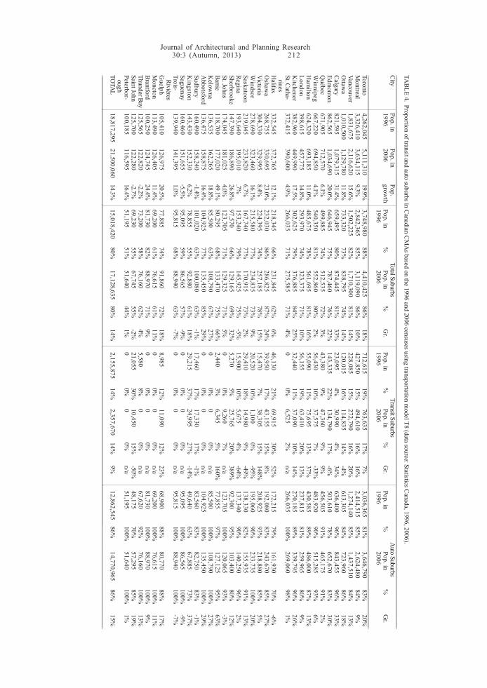
Journal of Architectural and Planning Research30:3 (Autumn, 2013) 212
TAB
LE 4. Proportion of transit and auto suburbs in Canadian C
MA
s based on the 1996 and 2006 censuses using transportation model T8 (data source: Statistics C
anada, 1996, 2006)._______________________________________________________________________________________________________________________________________________________________________________________________________________________________________________________________________________________________________________________________________________________________C
ityPop. in
Pop. inPop.
Total Suburbs Transit Suburbs
Auto Suburbs
19962006
growth
Pop. in%
Pop. in%
Gr.
Pop. in%
Pop. in%
Gr.
Pop. in%
Pop. in%
Gr.
19962006
19962006
19962006
_______________________________________________________________________________________________________________________________________________________________________________________________________________________________________________________________________________________________________________________________________________________________Toronto
4,262,0455,111,310
19.9%3,748,980
88%4,410,425
86%18%
712,61519%
763,63517%
7%3,036,365
81%3,646,790
83%20%
Montreal
3,326,4103,634,115
9.3%2,842,365
85%3,119,090
86%10%
427,85015%
494,61016%
16%2,414,515
85%2,624,480
84%9%
Vancouver1,831,675
2,116,62015.6%
1,502,22582%
1,710,30081%
14%228,085
15%272,790
16%20%
1,274,14085%
1,437,51084%
13%O
ttawa
1,010,5001,129,780
11.8%733,320
73%838,795
74%14%
120,01516%
114,83514%
-4%613,305
84%723,960
86%18%
Calgary821,595
1,079,31531.4%
659,49580%
874,44581%
33%23,095
4%30,990
4%34%
636,40096%
843,45596%
33%Edm
onton862,565
1,034,69020.0%
646,94575%
787,46076%
22%143,335
22%134,790
17%-6%
503,61078%
652,67083%
30%Q
uébec671,905
712,5706.1%
499,88574%
512,53572%
3%43,380
9%47,360
9%9%
456,50591%
465,17591%
2%W
innipeg667,220
694,8504.1%
540,35081%
552,86080%
2%56,430
10%37,575
7%-33%
483,92090%
515,28593%
6%H
amilton
624,320693,185
11.0%485,675
78%561,695
81%16%
55,09011%
75,69513%
37%430,585
89%486,000
87%13%
London398,615
457,77514.8%
293,97074%
323,37571%
10%56,155
19%63,410
20%13%
237,81581%
259,96580%
9%K
itchener382,960
449,99017.5%
302,62579%
376,88584%
25%32,440
11%37,090
10%14%
270,18589%
339,79590%
26%St. Catha-
372,415390,600
4.9%266,035
71%275,585
71%4%
00%
6,5252%
n/a266,035
100%269,060
98%1%
rinesH
alifax332,545
372,76512.1%
218,34566%
231,84562%
6%46,130
21%69,915
30%52%
172,21579%
161,93070%
-6%O
shawa
268,755330,695
23.0%232,030
86%286,825
87%24%
39,95017%
43,15515%
8%192,080
83%243,670
85%27%
Victoria304,330
329,9958.4%
224,39574%
257,18578%
15%15,470
7%38,305
15%148%
208,92593%
218,88085%
5%W
indsor278,690
323,46016.1%
215,58077%
234,83573%
9%20,520
10%1,100
0%-95%
195,06090%
233,735100%
20%Saskatoon
219,045233,820
6.7%167,740
77%170,915
73%2%
29,41018%
14,9809%
-49%138,330
82%155,935
91%13%
Regina
193,640195,010
.7%153,240
79%145,925
75%-5%
15,90010%
5,6754%
-64%137,340
90%140,250
96%2%
Sherbrooke147,390
186,89026.8%
97,57066%
129,16569%
32%5,270
5%25,765
20%389%
92,30095%
103,40080%
12%St. Johns
174,045181,025
4.0%123,705
71%129,325
71%5%
00%
9,2607%
n/a123,705
100%120,065
93%-3%
Barrie118,700
177,02049.1%
80,29568%
133,47075%
66%2,440
3%6,345
5%160%
77,85597%
127,12595%
63%K
elowna
136,535162,265
18.8%85,500
63%108,790
67%27%
00%
00%
n/a85,500
100%108,790
100%27%
Abbotsford
136,475158,875
16.4%104,925
77%135,450
85%29%
00%
00%
n/a104,925
100%135,450
100%29%
Sudbury160,490
158,240-1.4%
101,02063%
100,08063%
-1%17,460
17%17,330
17%-1%
83,56083%
82,75083%
-1%K
ingston143,430
152,3306.2%
78,85555%
92,88061%
18%29,215
37%24,995
27%-14%
49,64063%
67,88573%
37%Saguenay
160,460151,655
-5.5%95,095
59%86,565
57%-9%
00%
00%
n/a95,095
100%86,565
100%-9%
Trois-139,940
141,3951.0%
95,81568%
88,94063%
-7%0
0%0
0%n/a
95,815100%
88,940100%
-7% RivièresG
uelph105,410
126,97520.5%
77,88574%
91,86072%
18%8,985
12%11,090
12%23%
68,90088%
80,77088%
17%M
oncton113,490
126,40511.4%
69,20061%
76,61561%
11%0
0%0
0%n/a
69,200100%
76,615100%
11%Brantford
100,250124,745
24.4%81,730
82%88,970
71%9%
00%
00%
n/a81,730
100%88,970
100%9%
Thunder Bay125,565
122,820-2.2%
73,20058%
76,16062%
4%5,580
8%0
0%n/a
67,62092%
76,160100%
13%Saint John
125,700122,280
-2.7%69,230
55%67,745
55%-2%
21,05530%
10,45015%
-50%48,175
70%57,295
85%19%
Peterbor-100,185
116,59516.4%
51,19551%
51,64044%
1%0
0%0
0%n/a
51,195100%
51,640100%
1% oughTO
TAL
18,817,29521,500,060
14.3%15,018,420
80%17,128,635
80%14%
2,155,87514%
2,357,67014%
9%12,862,545
86%14,770,965
86%15%
_______________________________________________________________________________________________________________________________________________________________________________________________________________________________________________________________________________________________________________________________________________________________
Journal of Architectural and Planning Research30:3 (Autumn, 2013) 213
Suburbs in smaller cities — census agglomerationsCMAs accounted for 21.5 million people in 2006, or 68% of Canada’s population. However, another4.1 million Canadians live in smaller cities classified as census agglomerations (CAs). The popula-tions of these settlements range from 10,000-100,000 people, but only the larger CAs have the CTsneeded for our analysis. We took a sample of 10 CAs to estimate the proportion of suburbs in thiscategory using transportation model T8. The sample was not random; to control for regionalvariations, we deliberately selected CAs from each region of the country except Northern Canada(one from the Atlantic region, two from Québec, three from Ontario, two from the Prairies, and twofrom British Columbia).
The CAs we analyzed displayed characteristics similar to the smaller CMAs: a higher exurbanpopulation (23%), very little transit use, and a high proportion of auto suburbs. Extrapolating thesample forward, we estimate that another roughly 2.5 million Canadians live in the suburbs ofsmaller cities (see Table 5).
FINDINGS AND CONCLUSION
Canada is a suburban nation. In 2006, about 80% of the residents of Canadian metropolitan areaslived in suburbs, while only 12% lived in active core areas (Table 2). Moreover, this result probablyunderestimates the proportion of suburban residents, since at least half of the exurban residentscommute to central city jobs by automobile and live in single-family detached houses.
The proportions were relatively similar in 1996, but the growth rates were slightly different. Theactive cores of the CMAs grew by 21% from 1996-2006. At the same time, the suburbs grew by 14%,the same rate at which the CMAs grew overall. The exurban areas grew by only 8%, somewhat lessthan the CMA average. We should not infer too much from these growth rates, but it appears thatthe downtown building boom in the larger metropolitan areas may be growing at a slightly fasterrate than greenfield suburban development. However, we should also note that the active cores,
TABLE 5. Active core, suburb, and exurban proportions of 10 sample Canadian CAs based on the 2006 censususing transportation model T8 (data source: Statistics Canada, 2006)._______________________________________________________________________________________________________________________________________________________________________________________________________________________________________________________________________________________________________________________________________________________________City Pop. in Active Core Total Suburb Transit Suburb Auto Suburb Exurban
2006 Pop. %* Pop. %* Pop. %** Pop. %** Pop. %*_______________________________________________________________________________________________________________________________________________________________________________________________________________________________________________________________________________________________________________________________________________________________Kamloops 92,735 16,675 18% 46,325 50% 6,535 14% 39,790 86% 29,735 32%Belleville 91,380 22,170 24% 41,835 46% 0 0% 41,835 100% 27,375 30%Fredericton 85,725 13,025 15% 42,575 50% 7,435 17% 35,140 83% 30,125 35%Prince 83,275 19,170 23% 39,615 48% 0 0% 39,615 100% 24,490 29% GeorgeRed Deer 82,750 10,635 13% 72,115 87% 0 0% 72,115 100% 0 0%Sault Ste. 80,135 8,815 11% 57,525 72% 7,065 12% 50,460 88% 13,795 17% MarieDrummond- 78,080 15,255 20% 46,155 59% 0 0% 46,155 100% 16,670 21% villeMedicine 68,805 0 0% 56,580 82% 0 0% 56,580 100% 12,225 18% HatGranby 68,280 20,970 31% 33,955 50% 0 0% 33,955 100% 13,355 20%North Bay 63,460 6,115 10% 41,390 65% 3,675 9% 37,715 91% 15,955 25%Sample 794,625 132,830 17% 478,070 60% 24,710 5% 453,360 95% 183,725 23% totalsEstimated 4,150,095 693,732 17% 2,496,820 60% 129,053 5% 2,367,767 95% 959,542 23% totals for all CMAs_______________________________________________________________________________________________________________________________________________________________________________________________________________________________________________________________________________________________________________________________________________________________Note. * = percentage of total population; ** = percentage of total suburban population. Percentages may not addup to 100 due to rounding._______________________________________________________________________________________________________________________________________________________________________________________________________________________________________________________________________________________________________________________________________________________________

Journal of Architectural and Planning Research30:3 (Autumn, 2013) 214
which are promoted as offering a sustainable lifestyle, still only comprise perhaps 12% of themetropolitan population. Almost 80% of the metropolitan growth in the previous decade took placein the suburbs, as more than 2 million Canadians moved into these areas.
The results show that the characteristics of an active core may not be confined to the geographiccenter of metropolitan areas. By detaching the concept of the active core from the spatial classifi-cation of the inner city, we allow for the possibility of other cores embedded in a polynuclearmetropolitan structure. This flexibility fits more modern models of urban geography (Bunting, etal., 2002; Yang, et al., 2012) and recent planning movements to create suburban town centers andtransit-oriented developments (Filion and McSpurren, 2007).
To estimate the proportion of Canadians who lived in suburbs in 2006, we start by adding thesuburban populations of the CMAs and CAs from Tables 2 and 5:
CMA suburbs + CA suburbs = Total suburbs17,128,635 (87%) + 2,496,820 (13%) = 19,625,455 (100%)
One could argue that at least half of the exurban population is essentially very low density subur-ban, since the periphery of the metropolitan area is defined by the area where more than 50% of thelabor force is commuting to the central city and few are engaged in agriculture (Bollman, 2007).These trips are overwhelmingly taken by automobile, and housing in the exurban CTs mostlyconsists of single-family detached dwellings. Thus, it seems reasonable to allocate at least half ofthe exurban population of the CMAs and CAs to the total suburban population:
CMA exurban areas + CA exurban areas = Total exurban areas1,732,550 (64%) + 959,542 (36%) = 2,692,092 (100%)
50% exurban areas + Total suburbs = Total estimated 2006 suburban population1,346,046 + 19,625,455 = 20,971,501
The total national population in 2006 was 31,612,897 (Statistics Canada, 2006). Therefore, suburbsaccounted for 66% of the Canadian population in 2006. Even if we assume that the remainingCanadian population is rural, Canada’s suburban population must be approximately 21 millionpeople, or two-thirds of the total national population. This is a conservative estimate becausemany small town (less than 10,000 people) residents also live in suburban areas with extensiveautomobile use and low-density, single-family detached dwellings.
If two-thirds of Canada’s population currently lives in suburban neighborhoods, then plans forinfrastructure programs, environmental sustainability, public health, land use, and communitydesign should take this phenomenon into account. Future researchers of these issues may wish touse a more refined understanding of the active core, suburban, and exurban components of metro-politan areas.4 Even if urban development trends were to become significantly more intense, thecurrent suburban neighborhoods will comprise the bulk of the housing stock well into the 21stcentury. Thus, it appears that Canada is destined to remain a suburban nation in the decades ahead.
NOTES
1. The age of the dwelling is self-reported by the occupants, which can lead to some errors in the data (Baer,1990). Thanks to an anonymous reviewer for pointing this out.
2. However, since active transportation use in some smaller Canadian cities is quite low, this proportionalmethod allowed the possibility of nonsensical results in some CMAs. For example, only 3.9% of all employeesin Abbotsford, British Columbia, use active transportation to get to work. Thus, using this threshold, an Abbots-ford neighborhood that showed 6% active transportation and 94% auto use would be considered an active core.
Journal of Architectural and Planning Research30:3 (Autumn, 2013) 215
To avoid the anomalies created by this condition, we only classified a CT as an active core if its activetransportation rate was also at least 50% higher than the national average in 2006, or 10.65% (Turcotte andRuel, 2008).
3. Transit-use rates are usually fairly low in many smaller Canadian cities. In several of the smaller CMAs, thetransit-use rates in proposed transit suburbs may be absurdly low using this classification. For example, the 2006transit modal split in the Abbotsford CMA was 1.8%. Therefore, using this threshold, CTs with transit-use ratesof just 2.7% (150% of the CMA average) could be classified as transit suburbs. This could lead to a neighborhoodwith over 97% automobile use being obviously misclassified as a transit suburb. To avoid this difficulty, we onlyclassified a CT as a transit suburb if its transit modal split also exceeded 50% of the national average, or 7.5%(Turcotte and Ruel, 2008). Unlike with the active core threshold, there are few CTs with high rates of thevariable; therefore, 50% was not too restrictive and still had the desired effect of requiring the CT to reach acertain threshold.
4. Future researchers who wish to use the CT classifications discussed in this paper may download the spread-sheets from links provided at the Atlas of Suburbanisms website (http://env-blogs.uwaterloo.ca/atlas/?page_id=4027). We hope these classification models may yield more refined analyses of the urban/suburbandifferences than the previous practice of using municipal political boundaries or the first half of the postal code.
REFERENCES
Artibise A (1988) Canada as an urban nation. Daedalus 117(4):237-264.
Baer W (1990) Aging of the housing stock and components of inventory change. In D Myers (Ed.),Housing demography: Linking demographic structure and housing markets. Mad-ison: University of Wisconsin Press, pp. 249-273.
Bagley MN, Mokhtarian PL, Kitamura R (2002) A methodology for the disaggregate, multidimen-sional measurement of residential neighbourhood type. Urban Studies 39(4):689-704.
Beauregard RA (2006) When America became suburban. Minneapolis: University of MinnesotaPress.
Boarnet M, Crane R (2001) Travel by design: The influence of urban form on travel. New York:Oxford University Press.
Bollman RD (2007) The demographic overlap of agriculture and rural (Statistics Canada cata-logue no. 21-601-MIE, Agriculture and rural working paper series no. 81). Ottawa:Statistics Canada Agriculture Division.
Bourne L (2001) The urban sprawl debate. Plan Canada 41(4):26-28.
Bourne L, Ley D (1993) The changing social geography of Canadian cities. Montreal: McGill-Queen’s Press.
Bruegmann R (2005) Sprawl: A compact history. Chicago: University of Chicago Press.
Bunting T, Filion P (1999) Dispersed city form in Canada: A Kitchener CMA case example. TheCanadian Geographer 43(3):268-287.
Bunting T, Filion P, Priston H (2002) Density gradients in Canadian metropolitan regions, 1971-96:Differential patterns of central area and suburban growth and change. Urban Stud-ies 39(13):2531-2552.
Burchell RW, Lowenstein G, Dolphin WR, Galley CC, Downs A, Seskin S, Still KG, Moore T (Eds.)(2002) Costs of sprawl — 2000 (Transit Cooperative Research Program report 74).Washington, DC: National Academy Press.

Journal of Architectural and Planning Research30:3 (Autumn, 2013) 216
The Canadian Press (2012) Country living continues to decline as majority of Canadians live in bigcities. Guelph Mercury 8 February. http://www.guelphmercury.com/news-story/2777855-country-living-continues-to-decline-as-majority-of-canadians-live-in-big-cities/. Site accessed 12 July 2013.
Christens B (2009) Suburb decentralization and the new urbanism: A pragmatic inquiry into value-based claims. Journal of Architectural and Planning Research 26(1):30-43.
Crane R (2000) The influence of urban form on travel: An interpretive review. Journal of PlanningLiterature 15(1):3-23.
du Plessis V, Beshiri R, Bollman RD, Clemenson H (2001) Definitions of rural. Rural and Small TownCanada Analysis Bulletin 3(3):1-17 (Statistics Canada catalogue no. 21-006-XIE).http://www.statcan.gc.ca/pub/21-006-x/21-006-x2001003-eng.pdf. Site accessed12 July 2013.
du Plessis V, Beshiri R, Bollman RD, Clemenson H (2002) Definitions of “rural” (Statistics Canadacatalogue no. 21-601-MIE, Agriculture and rural working paper series no. 61). http://www.statcan.gc.ca/pub/21-601-m/2002061/4224867-eng.pdf. Site accessed 12 July2013.
Duany A, Plater-Zyberk E, Speck J (2000) Suburban nation: The rise of sprawl and the decline ofthe American dream. New York: North Point Press.
Ewing R, Cervero R (2001) Travel and the built environment: A synthesis. Transportation ResearchRecord 1780:87-114.
Ewing R, Cervero R (2010) Travel and the built environment: A meta-analysis. Journal of theAmerican Planning Association 76(3):265-294.
Filion P (2001) Suburban mixed-use centres and urban dispersion: What difference do they make?Environment and Planning A 33(1):141-160.
Filion P, Bunting T (2006) Understanding twenty-first century urban structure: Sustainability,unevenness, and uncertainty. In T Bunting and P Filion (Eds.), Canadian cities intransition: Local through global perspectives, 3rd edition. Toronto: Oxford Univer-sity Press, pp. 1-23.
Filion P, Hammond K (2003) Neighbourhood land use and performance: The evolution of neigh-bourhood morphology over the 20th century. Environment and Planning B: Plan-ning and Design 30(2):271-296.
Filion P, McSpurren K (2007) Smart growth and development reality: The difficult co-ordination ofland use and transport. Urban Studies 44(3):501-523.
Filion P, McSpurren K, Appleby B (2006) Wasted density? The impact of Toronto’s residential-density-distribution policies on public-transit use and walking. Environment andPlanning A 38(7):1367-1392.
Filion P, McSpurren K, Bunting T, Tse A (2004) Canada-U.S. metropolitan density patterns: Zonalconvergence and divergence. Urban Geography 25(1):42-65.
Forsyth A (2012) Defining suburbs. Journal of Planning Literature 27(3):270-281.
Journal of Architectural and Planning Research30:3 (Autumn, 2013) 217
Frank L, Frumkin H (2004) Urban sprawl and public health: Designing, planning, and buildingfor healthy communities. Washington, DC: Island Press.
Friedman A (2002) Planning the new suburbia: Flexibility by design. Vancouver: UBC Press.
Galster G, Hanson R, Ratcliffe M, Wolman H, Coleman S, Freihage J (2001) Wrestling sprawl to theground: Defining and measuring an elusive concept. Housing Policy Debate 12(4):681-718.
Gans HJ (1968) Urbanism and suburbanism as ways of life: A re-evaluation of definitions. InHJ Gans (Ed.), People and plans: Essays on urban problems and solutions. NewYork: Basic Books, pp. 41-64.
Gordon DLA, Vandyk C (2010) Suburban national capital: A pilot study of Canada’s post-1945suburbs in Ottawa-Hull. Paper presented at the 14th International Planning HistorySociety Conference, “Urban Transformation: Controversies, Contrasts and Chal-lenges.” Istanbul (12-15 July).
Gordon DLA, Vipond S (2005) Gross density and new urbanism: Comparing conventional and newurbanist suburbs in Markham, Ontario. Journal of the American Planning Associa-tion 71(2):41-54.
Gordon P, Richardson H (1997) Are compact cities a desirable planning goal? Journal of theAmerican Planning Association 63(1):95-106.
Grant J (1999) Can planning save the suburbs? Plan Canada 30(4):16-18.
Grant J (2006a) Planning the good community: New urbanism in theory and practice. New York:Routledge.
Grant J (2006b) Promises and prospects: New urbanism in practice (Working paper). http://theoryandpractice.planning.dal.ca/pdf/suburbs/working_papers/promises_prospects.pdf. Site accessed 12 July 2013.
Grant J (2007) An American effect: Contextualizing gated communities in Canadian planning prac-tice. Canadian Journal of Urban Research 16(1):1-19.
Grant J, Greene K, Maxwell K (2004) The planning and policy implications of gated communities.Canadian Journal of Urban Research 13(1):70-88.
Hancock M (1994) Don Mills: A paradigm of community design. Plan Canada July(Special issue):87-90.
Harris R (1996) Unplanned suburbs: Toronto’s American tragedy, 1900 to 1950. Baltimore: JohnsHopkins University Press.
Harris R (2004) Creeping conformity: How Canada became suburban, 1900-1960. Toronto: Uni-versity of Toronto Press.
Harris R, Larkham PJ (1999) Changing suburbs: Foundation, form, and function. London: Rout-ledge.
Hayden D (2003) Building suburbia green fields and urban growth, 1820-2000. New York: Vin-tage.

Journal of Architectural and Planning Research30:3 (Autumn, 2013) 218
Heisz A, Larochelle-Côté S (2005) Work and commuting in census metropolitan areas, 1996-2001(Statistics Canada catalogue no. 89-613-MIE, no. 007). Ottawa: Statistics CanadaBusiness and Labour Market Analysis Division.
Hodge G, Gordon D (2013) Planning Canadian communities: An introduction to the principles,practice and participants, 6th edition. Toronto: Nelson Education Limited.
Katz B, Lang RE (2003) Redefining urban and suburban America: Evidence from census 2000.Washington, DC: Brookings Institution Press.
Kunstler JH (1993) The geography of nowhere: The rise and decline of America’s man-madelandscape. New York: Simon and Schuster.
Leung HL (2003) Land-use planning made plain, 2nd edition. Toronto: University of TorontoPress.
Levinson D, Kumar A (1997) Density and the journey to work. Growth and Change 28(2):147-172.
Ley D, Frost H (2006) The inner city. In T Bunting and P Filion (Eds.), Canadian cities in transi-tion: Local through global perspectives, 3rd edition. Toronto: Oxford UniversityPress, pp. 192-210.
Litman T (2010) Evaluating public transit benefits and costs: Best practices guidebook. Victoria,BC: Victoria Transit Policy Institute.
MacGregor R (2009) City slickers and the legend of Canada as an urban nation. The Globe andMail 9 November:A2.
Martel L, Caron Malenfant É (2007) Portrait of the Canadian population in 2006: Findings, 2006census analysis series (Statistics Canada catalogue no. 97-550-XIE). Ottawa: Statis-tics Canada Demography Division.
McCall D (2009) 2006 census housing series: Issue 5 — Canada’s census metropolitan areas (CMAs)(Research highlight socio-economic series paper no. 09-022). Ottawa: Canada Mort-gage and Housing Corporation.
McCann LD (1996) Planning and building the corporate suburb of Mount Royal, 1910-1925. Plan-ning Perspectives 11(3):259-301.
McCann LD (1999) Suburbs of desire: Shaping the suburban landscape of Canadian cities, 1900-1950. In H Richard and P Larkham (Eds.), Changing suburbs — foundation, form andfunction. London: Routledge, pp. 111-145.
McCann LD, Smith PJ (1991) Canada becomes urban: Cities and urbanization in an historical per-spective. In T Bunting and P Filion (Eds.), Canadian cities in transition: Localthrough global perspectives, 1st edition. Toronto: Oxford University Press, pp. 69-99.
Mendelson R (2001) Geographic structures as census variables: Using geography to analysesocial and economic processes (Statistics Canada catalogue no. 92F0138MIE, Ge-ography working paper series no. 2001-1). Ottawa: Statistics Canada GeographyDivision.
Millward H (2008) Evolution of population densities: Five Canadian cities, 1971-2001. Urban Geog-raphy 29(7):616-638.
Journal of Architectural and Planning Research30:3 (Autumn, 2013) 219
Muller P (2004) Transportation and urban form: Stages in the spatial evolution of the Americanmetropolis. In S Hanson and G Giuliano (Eds.), The geography of urban transporta-tion, 3rd revised edition. New York: Guilford Press, pp. 59-85.
The Ohio State University (2002) Exurban change program — Ohio maps. http://exurban.osu.edu/maps_ohio.htm#By%20Density. Site accessed 30 November 2009.
Parr JB (2007) Spatial definitions of the city: Four perspectives. Urban Studies 44(2):381-392.
Pushkarev B, Zupan J (1977) Public transportation and land use policy. Bloomington: IndianaUniversity Press.
Sewell J (1993) The shape of the city: Toronto struggles with modern planning. Toronto: Univer-sity of Toronto Press.
Smith PJ (2006) Suburbs. In T Bunting and P Filion (Eds.), Canadian cities in transition: Localthrough global perspectives, 3rd edition. Toronto: Oxford University Press,pp. 211-233.
Song Y, Knapp G (2007) Quantitative classification of neighbourhoods: The neighbourhoods ofnew single-family homes in the Portland metropolitan area. Journal of Urban Design12(1):1-24.
Statistics Canada (1996) 1996 census of Canada: Profile data. Ottawa and Vancouver: StatisticsCanada and Tetrad Computer Applications.
Statistics Canada (2001) 2001 census of Canada: Profile data. Ottawa and Vancouver: StatisticsCanada and Tetrad Computer Applications.
Statistics Canada (2006) 2006 census of Canada: Profile data. Ottawa and Vancouver: StatisticsCanada and Tetrad Computer Applications.
Stone LO (1967) Urban development in Canada. Ottawa: Dominion Bureau of Statistics.
Talen E (2003) Measuring urbanism: Issues in smart growth research. Journal of Urban Design8(3):195-215.
Talen E (2012) Sprawl retrofit: A strategic approach to parking lot repair. Journal of Architecturaland Planning Research 29(2):113-132.
Torrens P (2008) A toolkit for measuring sprawl. Applied Spatial Analysis 1(1):5-36.
Turcotte M (2008a) Life in metropolitan areas: Dependence on cars in urban neighbourhoods.Canadian Social Trends (Statistics Canada) 85(Summer):20-30.
Turcotte M (2008b) Life in metropolitan areas: The city/suburb contrast: How can we measure it?Canadian Social Trends (Statistics Canada) 85(Summer):2-19.
Turcotte M (2009) Life in metropolitan areas: Are suburban residents really less physically active?Canadian Social Trends (Statistics Canada) 87(Summer):32-41.
Turcotte M, Ruel J (2008) Commuting patterns and places of work of Canadians, 2006 census(Statistics Canada catalogue no. 97-561-XIE). Ottawa: Statistics Canada.

Journal of Architectural and Planning Research30:3 (Autumn, 2013) 220
Walks A (2004) Place of residence, party preferences, and political attitudes in Canadian cities andsuburbs. Journal of Urban Affairs 26(3):269-295.
Walks A (2005) The city-suburban cleavage in Canadian federal politics. Canadian Journal ofPolitical Science 38(2):383-413.
Walks A (2007) The boundaries of suburban discontent? Urban definitions and neighbourhoodpolitical effects. The Canadian Geographer 51(2):160-185.
Yang J, French S, Holt J, Zhang X (2012) Measuring the structure of U.S. metropolitan areas, 1970-2000. Journal of the American Planning Association 78(2):197-209.
Additional information may be obtained by writing directly to Dr. Gordon at Robert SutherlandHall, Room 534, School of Urban and Regional Planning, Queen’s University, Kingston, ON, Can-ada K7L 3N6; email: [email protected].
ACKNOWLEDGMENTSThe research for this paper was funded by the Social Sciences and Humanities Research Council of Canada.Research assistants included Angus Beaty, Mehdi Bouhadi, Mathieu Cordary, Anthony Hommik, Benjamin Jean,Devon Miller, Andrew Morton, Michelle Nicholson, Tyler Nightingale, Thierry Pereira, Krystal Perepeluk,Julien Sabourault, Jennifer Sandham, Isaac Shirokoff, Amanda Slaunwhite, and Chris Vandyk. Peer reviewersincluded Ajay Agarwal, Pierre Filion, Jill Grant, Richard Harris, Paul Hess, Nik Luka, Martin Turcotte, and AndrejsSkaburskis, but the authors are responsible for any errors or omissions.
AUTOBIOGRAPHICAL SKETCHES
David Gordon is Professor and Director of the School of Urban and Regional Planning at Queen’s University inKingston, Ontario. He received a doctorate from the Harvard Graduate School of Design in 1994. His currentresearch examines the extent of Canadian suburbs and the planning history of Canada’s capital city.
Mark Janzen is a policy analyst for the British Columbia Ministry of Transportation and Infrastructure inVictoria, British Columbia. He received a Master’s degree in Planning from the Queen’s School of Urban andRegional Planning in 2011.
Manuscript revisions completed 19 July 2013.
Copyright © 2013, Locke Science Publishing Company, Inc.Chicago, IL, USA All Rights Reserved
Journal of Architectural and Planning Research30:3 (Autumn, 2013) 221
PLANNING, DESIGN, AND RELIGION: AMERICA’SCHANGING URBAN LANDSCAPE
Sanjoy MazumdarShampa Mazumdar
In the study of cities, the significance of religion has fluctuated over time. In the recent past,religion has not been a major concern for planners and designers, and today there are fewwritings on religion in planning, and little is taught on the subject in academic planningdepartments. Is it important to consider religion in planning in the United States? This paperdescribes the changing religious landscape in the U.S. along with the various ways religion isbeing expressed. We describe five areas in which religion currently interfaces with public lifeand impacts urban design: religious communities and neighborhoods, religious institutions andstructures, religious use of public space, religion and housing, and religion and health. We alsodiscuss why planners and designers should consider religion as potentially salient. Theconclusion summarizes the major issues for planners and designers in a multi-religious society;offers a few caveats; delineates the consequences of neglecting religion; and providesrecommendations, including a special religious sensibility, a multi-faith approach, andpragmatic strategies and actions.