PCA R&D Serial No. 2486

Sulfate Resistance of Concrete: A New Approach

by Chiara F. Ferraris, Paul E. Stutzman, and Kenneth A. Snyder

Published by PCA in 2006 without copyright.

i

KEYWORDS External sulfate attack, cement paste, mortar, expansion, modulus of elasticity, cycles wet-dry, diffusion, sorption ABSTRACT The objective of this program is to critically review existing performance specifications and test methods on sulfate attack, to provide the technical basis for improved performance standards, and to provide criteria for evaluation, selection, and use of concrete materials for sulfate attack resistance. The approach taken is based on ASTM E 6321. In following the procedure described in ASTM E 632, the performance of concrete under sulfate attack needs to be divided into several phenomena and therefore several tests had to be developed. The various phenomena are: • Concrete properties: absorption and diffusion of sulfate (resistance to the ingress of sulfate

solutions). • Cement paste properties: chemical reaction between the hydration product and the sulfate

ions. In the literature this is referred as chemical attack [2]. • Influence of environmental conditions: type of immersion (constant, partial, or cyclic) and

temperature. In the literature, this is referred as physical attack [2]. Therefore the tests that were developed are: • Absorption of water by a concrete specimen. This test was submitted to ASTM and approved

in 2004 as ASTM C 1585. • Diffusion of sulfate in saturated specimens. A methodology to modify existing methods is

given. • A specimen test to determine the cement’s resistance to sulfate attack, which is three to five

times shorter than current tests. • A test to determine the resistance to sulfate attack when a concrete is not totally immersed in

the solution. This report also provides guidelines on how to combine the results of all these tests to determine a concrete’s sulfate resistance (see section Approach overview). REFERENCE Ferraris, C. F.; Stutzman, P.E., and Snyder, K. A., Sulfate Resistance of Concrete: A New Approach, R&D Serial No. 2486, Portland Cement Association, Skokie, Illinois, USA, 2006, 93 pages.

1 This standard was withdrawn in 2005 because it was not used; however, it was active when we started working on this project in 1999. We believe that this standard offers good guidelines to develop accelerated tests.

ii

Table of Contents Page Introduction......................................................................................................................... 1 Approach overview............................................................................................................. 2 Concrete Characteristics ..................................................................................................... 5

Diffusion ......................................................................................................................... 6 Introduction................................................................................................................. 6 Transport equation ...................................................................................................... 7

Species flux............................................................................................................. 7 Electrostatic interactions......................................................................................... 8 Characterizing parameters ...................................................................................... 9

Porosity ....................................................................................................................... 9 Formation factor.......................................................................................................... 9 Moisture content ....................................................................................................... 10 Experimental procedure ............................................................................................ 10

Capillary porosity.................................................................................................. 11 Concrete conductivity ........................................................................................... 11 Pore solution conductivity .................................................................................... 12 CEMHYD3D ........................................................................................................ 14

Practical examples .................................................................................................... 14 Absorption..................................................................................................................... 15

Preconditioning of the specimen............................................................................... 16 Test method description............................................................................................ 18 Status......................................................................................................................... 22

Wet-dry Cycles ............................................................................................................. 22 Background............................................................................................................... 23

Crystallization pressure......................................................................................... 23 Principle of tests........................................................................................................ 27 Experimental setup.................................................................................................... 27 Results....................................................................................................................... 28

Concrete specimens .............................................................................................. 28 Mortar specimens.................................................................................................. 30

Summary ................................................................................................................... 36 Future work............................................................................................................... 36

Transport Properties-based Models .............................................................................. 36 NIST CONCLIFE [56] ............................................................................................. 37 Mobasher-Tixier Model ............................................................................................ 39 STADIUM ................................................................................................................ 40 Summary of the models ............................................................................................ 40

Cement Characteristics ..................................................................................................... 41 Introduction................................................................................................................... 41 Tests performed ............................................................................................................ 42

Materials used ........................................................................................................... 42 Specimens prepared .................................................................................................. 46 Measurements on mortar prisms............................................................................... 47

Microstructure observations.......................................................................................... 58

iii

The Scanning Electron Microscope (SEM) .............................................................. 58 X-ray Powder Diffraction Analysis (XRD) .............................................................. 61

Small prisms new test ................................................................................................... 63 Experimental setup for the proposed method ........................................................... 65 Results and discussion .............................................................................................. 69 Precision statement of this method ........................................................................... 71 Conclusion ................................................................................................................ 72

Conclusions....................................................................................................................... 73 Acknowledgements........................................................................................................... 73 References......................................................................................................................... 74 Appendix A: Standard Test Method for measuring the Sulfate Resistance of Hydraulic Cements ............................................................. A-1

iv

List of Figures Figure 1: Flow chart for determination of the sulfate resistance of concrete or cement paste. Each

box in bold corresponds to a chapter of this report..................................................... 5 Figure 2 [37]: Relative humidity achieved after the various preconditionings. The main

difference is the time spent in the environmental chamber at 50°C and 80% RH. T1: no time; T2: 24 hours; T3: 48 hours; T4: 3 days; T5: 7 days; T6: until constant mass; T7: until constant mass at 20°C and 80% RH. The error bars represent one standard deviation.17

Figure 3 [37]: RH of the air inside the conditioning containers versus time. Each curve represents measurements on a concrete cylinder. Each point is the average of data on three slices of a concrete cylinder. The error bars represent one standard deviation. ........................ 18

Figure 4: Comparison of sorption measured by capillary and by ponding. A) The water content per surface area versus linear time as measured, B) the water content per surface area vs. square root of time for the first 7 hours. These are results for one samples and no uncertainty was calculated as they are given only as an example of results that could be obtained..................................................................................................................... 19

Figure 5: Schematic of capillary sorption test .................................................................. 20 Figure 6: Schematic of ponding sorption test ................................................................... 20 Figure 7: Pictures of observed leaks with improper sealing: A) water leaked between the two

layers of tape, B) water has leaked in between the tape and the specimen sides and is wetting the bottom (nontested surface)..................................................................... 21

Figure 8: Calculation of the sorption coefficient .............................................................. 22 Figure 9: Schematic of the specimen setup for the wet-dry cycles................................... 28 Figure 10: Marking of the specimens for measurements.................................................. 28 Figure 11: Picture of concrete submitted to the wet-dry deterioration after 25 weeks. D =

deteriorated zone. The diameter of the specimens is 50 mm (2 in.) and the height is 101 mm (4 in.)......................................................................................................................... 29

Figure 12: Expansion (A) and modulus of elasticity (B) of prisms made with the same composition as shown in Table 8. All data for the expansion are an average of three specimens. The modulus is the average of two specimens. The error bars represent the one standard deviation in both graphs. The expansion of the control is measured with only two specimens after 360 days (the third specimen broke). .............................................. 31

Figure 13: Deterioration width of the mortar specimens for set #1 at 25°C. The percentages in the legend are the RH used. ............................................................................................ 32

Figure 14: Relative expansion of the top and bottom diameters for mortar set #1. The percentages in the legend are the RH used. .................................................................................. 33

Figure 15: Deterioration width of the mortar specimens for set #2 at 25°C. There are no data at 40°C because no deterioration was observed. The percentages in the legend are the RH used. The error bars are not shown for clarity but all data would be ± 20% (as seen in Figure 13). ............................................................................................................................ 33

Figure 16: Relative expansion of the top and bottom diameters for set #2 at 25°C. The percentages in the legend are the RH used. The error bars are very large when the specimens start deteriorating..................................................................................... 34

Figure 17: Relative expansion of the top and bottom diameters for set #2 at 40°C. ........ 34 Figure 18: Basic screen for sulfate attack service life computation. ................................ 38

v

Figure 19: XRD patterns from a bulk and salicyclic acid-methanol extraction residue for cement Type I/II cement (NIST Code #PCA-12). (Y-axis is densities intensity, X-axis represents degrees 2-theta for Cu Kα radiation)......................................................................... 43

Figure 20: XRD patterns for bulk (upper) and salicyclic acid-methanol extraction residue for cement Type V (NIST Code # PCA-16). (Y-axis is densities intensity, X-axis represents degrees 2-theta for Cu Kα radiation)......................................................................... 44

Figure 21: Expansion of the specimens in set #1. A) All data, B) expansion of the specimens in set #1 prepared with Type V cement. This is an expanded view of A. The crosses indicate that specimens broke and therefore the average is over a smaller number of specimens. After the second cross, no more specimens were available that were exposed to magnesium sulfate. The limewater curve is given for information only as it is not from the same cement or mix design............................................................................................................. 49

Figure 22: Modulus of elasticity for set #1. The standard deviation is not shown but it was found to be less than ± 0.3 GPa........................................................................................... 50

Figure 23: Specimens in limewater for set #2. ................................................................. 51 Figure 24: Expansion of the specimens in set #2, curing method A. A) All data, B) close-up view

of expansion below 0.25% for specimens of set #2 (A). The “Expansion in lime” shows the expansion for the specimens kept in limewater. The values of the expansion in lime later than 300 days are an extrapolation (see text)............................................................ 52

Figure 25: Expansion of set #2, after about 300 days curing in limewater (curing B). A) All data B) closeup view of expansion below 0.25% for specimens of set #2 (A). The “Expansion in lime” shows the expansion for the specimens kept in lime water. The values of the expansion in lime later than 300 days are an extrapolation (see text). ..................... 53

Figure 26: Modulus of elasticity for set #2 in sodium sulfate curing method A. The standard deviation is not shown but it was found to be less than ± 0.3 GPa........................... 55

Figure 27: Modulus of elasticity of the specimens of set #2 after curing method B (almost 300 days). The standard deviation is not shown but it was found to be less than ± 0.3 GPa.................................................................................................................................... 55

Figure 28: ASTM C 1012 Expansion data from the independent laboratory: A) Cement Type I and Type II/V, B) blended cements and the control represented by the cement Type I ................................................................................................................................... 57

Figure 29: 0.45 w/c, 7 days old hardened cement paste (field width, 25 μm)................ 59 Figure 30: Energy-dispersive x-ray spectrum of calcium-silicate-hydrate indicates the presence

of calcium, silicon, magnesium, aluminum, and sulfur. ........................................... 60 Figure 31: After 64 days of exposure, backscattered electron images at low magnification (lower

left) and higher magnification (lower right) and X-ray images for sulfur (upper left), and calcium (upper right) show the cracking below the surface and gypsum (CaSO4·2H2O) filling cracks. The surface is oriented toward the left. (Scale indicated in the figures.) 62

Figure 32: Cross section of hardened cement paste not exposed to sulfate solution, showing residual cement grains, calcium hydroxide (CH), calcium-silicate-hydrate (CSH), monosulfate (AFm), and voids. ................................................................................ 63

vi

Figure 33: Type I/II cement paste (105 days of exposure to sulfate solution), Na2SO4-soaked specimen, showing increased porosity near the surface (left, zone 1), loss of calcium hydroxide in outer 150 μm (zones 1 & 2), possible densification of inner-product CSH in CH-depleted zone 2, deposition of gypsum in place of CH, and replacement of monosulfate with ettringite. ........................................................................................................... 63

Figure 34: Composite image with about 12 mm total field width with the backscattered electron image of the mortar and end pin (bright rod) and above X-ray images of sulfur highlighting gypsum-filled cracks in the mortar. The gap at the base of the pin is about 0.5 mm in width.................................................................................................................................... 65

Figure 35: Molds for specimens: A) general view, B) pin imbedded in the specimen, C) screw to hold pins in place during cast.................................................................................... 67

Figure 36: Specimens with epoxy coated ends, Specimen D was also coated 5 mm on the side; Specimen A had only the ends sections coated. It was determined that the D-type coating gave more reproducible results [67] ......................................................................... 68

Figure 37: Expansion measurement: A) reference and a specimen, B) comparator with the reference in place. ..................................................................................................... 68

Figure 38: Average expansion of small specimen versus time: A) mortar specimens, B) cement paste specimens. The standard deviations of the five specimens are shown as error bars.................................................................................................................................... 70

Figure 39: Average expansion of large specimens versus time. The standard deviations of the three specimens are shown as error bars. For FA-C, the error bars are smaller than the data symbol....................................................................................................................... 70

Figure 40: Expansion of cement paste for determination of reproducibility. A and B are identical cement and single operator and laboratory. .............................................................. 71

Figure 41: Average curve of data shown in Figure 40...................................................... 72 Figure 42: Specimen mold schematic (SI units). For these molds the gage value measured was

24.48 mm (distance between the pin tips inside the specimen).............................. A-6 Figure 43: Specimens curing with epoxy coated ends.................................................... A-7

vii

List of Tables Table 1: Experimental Methods for Estimating the Porosity and the Formation Factor of

Concrete .................................................................................................................... 10 Table 2: Equivalent Conductivity at Infinite Dilution o

iλ and Conductivity Coefficient iG at 25oC........................................................................................................................... 13

Table 3: Scenarios for Estimating the Porosity and Formation Factor of Concrete Specimens................................................................................................................................... 14

Table 4: Recommended Methods for Determining the Pore Solution and Concrete Conductivities when the Concrete Components and Concrete Mixture Design are Both Available 14

Table 5: Recommended Methods for Determining the Pore Solution and Concrete Conductivities when a Physical Field Specimen and the Concrete Mixture Design are Both Available................................................................................................................................... 15

Table 6: Properties of Sodium and Magnesium Sulfate Salts [48]................................... 25 Table 7: Type of Exposure................................................................................................ 30 Table 8: Composition of the Specimens for Sets #1 and #2 ............................................. 30 Table 9: Initiation of Spalling on the Specimens.............................................................. 35 Table 10: Cement Oxide Compositions............................................................................ 45 Table 11: Compositional Estimates .................................................................................. 45 Table 12: Supplementary Cementitious Materials Used. ................................................. 46 Table 13: Specimens Prepared.......................................................................................... 47 Table 14: Age of the Specimens for the Inflection Point for Expansion and Modulus of Elasticity

for Set #1................................................................................................................... 50 Table 15: Duration of Curing for Method B..................................................................... 54 Table 16: Age of the Specimens for the Inflection Point for Expansion and Modulus of Elasticity

for Set #2................................................................................................................... 54 Table 17: Age of the Specimens for the Inflection Point for Expansion and Modulus of Elasticity

for Set #2................................................................................................................... 56 Table 18: X-ray Microanalysis Scheme........................................................................... 60 Table 19: Time in Days to Reach 0.1 % Expansion and Expansion at an Arbitrary Date 71

1

Sulfate Resistance of Concrete: A New Approach

by Chiara F. Ferraris, Paul Stutzman, and Kenneth Snyder *

INTRODUCTION Degradation of cementitious systems exposed to sulfate salts is the result of sulfate transport through the pore system, chemical reaction with the hydration product phases present, generation of stresses due to the creation of the expansive reaction products, and the mechanical response (typically spalling and cracking) of the bulk material due to these stresses. Each component of this process plays a unique role in the ultimate response of the concrete; change the material properties relevant to any one component and the concrete performance can change dramatically. Therefore, laboratory tests of ”sulfate attack'' that are based primarily on submerging the specimens in sulfate solution and then measuring some physical property, such as expansion, are effectively lumping all of these mechanisms into a single test. The result is a test that characterizes how a particular concrete performs under specific conditions. If the field conditions are different, the performance of the concrete can also be different.

Often, it is assumed that the performance of concrete regarding its resistance to external sulfate attack depends on the composition of the cement used. Therefore, most standard tests are based on measuring macroscopic properties of cement pastes or mortars, such as expansion, modulus of elasticity, or compressive strength. Depending on the values obtained, after a test duration of six months to a year (e.g., ASTM 1012 [1]), conclusions are drawn regarding the suitability of the cement tested to be used in a high sulfate environment. This approach lacks the mechanistic premises that could lead to a better determination of the important parameters that influence the severity and the kinetics of the attack.

Therefore, to predict the resistance to sulfate attack of a concrete, it is necessary to develop a protocol that takes into account the type of exposure and separates the various mechanisms. For instance, absorption of sulfate solution, diffusion of sulfates into the pore structure, and chemical reaction between the sulfates and the hydration products cannot all be tested in one measurement.

There are three types of tests that can be found in the literature [2, 3]: • Internal attack • External attack under constant exposure • Partial or cyclic exposure In this report we will concentrate on the external attack scenario with the specimen either

completely or partially immersed in the sulfate solution. A new protocol will be presented based

* Physicist, Physical Scientist, and Physicist respectively at National Institute of Standard and Technology, 100 Bureau Dr. MS 8615, Gaithersburg, MD 20899-8615; http://ciks.cbt.nist.gov/monograph.

2

on ASTM E 632. This study led to the development of four tests, one of which was already approved by ASTM. Future research needs will also be presented.

APPROACH OVERVIEW In a typical test as described in the literature [2, 3, 4], specimens are exposed to aqueous solutions of magnesium, calcium, or sodium sulfate of various concentrations. The temperature is controlled and the specimen may be exposed to wet/dry cycles, to partial immersion, or to continuous immersion. The extensive work done by the European Committee for Standardization (CEN) organization to improve expansion measurements [4] did not result in an accelerated test but in increased precision between different laboratories' data. Also, in attempting to reduce the duration, the environmental conditions of the test do not usually duplicate the conditions encountered in the field. Therefore, it is likely that the material response and service life might not be the same in the laboratory and in the field. Also, usually only the macroscopic deterioration, such as expansion or strength loss, etc., is measured over a prescribed period of time. If the deterioration is lower than a pre-set value, the cement is considered sulfate resistant. This approach could be misleading if the field conditions are not similar to the conditions of the laboratory experiment. Therefore, this methodology is not satisfactory because it is slow (most of the tests last six months to a year) and does not allow the estimation of specimen service life. Ideally, the goal of a laboratory test is to determine that X months in the laboratory will correspond to Y years of field performance. These relationships were never established for any of the currently available tests. Therefore, a new approach to determine the performance of cement and concrete is needed.

The approach adopted for this project is based on ASTM E 632 [5], a mechanistic approach. ASTM E 632 describes in a flow chart the steps needed to develop an accelerated test that can predict field performance of the material. The standard leads the designer to focus on the main causes of the degradation and to try to determine appropriate tests to measure the properties related. Therefore, the following questions need to be addressed first:

• Performance required • Degradation indicators • Degradation mechanisms • Environment • How degradation characteristics of in-use performance can be induced by accelerated

aging tests • Definition of performance requirements for predictive service life tests

The performance of a concrete specimen is determined by one or more of the following

properties: expansion, mass loss or spalling, and the loss of compressive and flexural strength with time. The degradation indicators of failure would be that one or more of the above performance properties is undesirably high, i.e., decrease in compressive and/or flexural strength, mass loss, or spalling or expansion of the specimen.

The timeline of the concrete degradation due to sulfate attack could be summarized in the following manner:

• Penetration of the sulfate ions into the specimen, either by absorption or by diffusion, depending on the saturation level of the specimen.

3

• Reaction of the sulfate ions with the cement hydration products to form gypsum and ettringite, or, in general, to modify the structure of C-S-H. This reaction leads to the destruction of the hydration products that constitute the backbone of the cement paste, which forms the matrix of the concrete. Different mechanisms are reported depending on the cations that are attached to the sulfate, e.g., Mg, Ca, or Na. A full description of the mechanisms of degradation is given in many publications [2].

The degree and the kinetics of the deterioration depend on environmental factors: • The sulfate content in the soil or water in contact with the concrete. • Whether the concrete is submitted to a wet/dry cycle or to constant immersion. For

instance, a tidal zone provides cycles of wetting and drying and can lead to deterioration by crystallization pressure in addition to that caused by chemical reaction between sulfate ions and hydration products.

• The unlimited availability of sulfate ions might increase the deterioration of the specimen. Any of the following types of exposure, such as flowing water, soil, seawater, and high relative humidity (RH), might change the extent and rate of the deterioration. Also, at least one study [6] has shown that the pH of the solution in contact with the structure has an influence on the mechanisms of deterioration.

From the preceding analysis of the problem, we can say that the properties to be determined

are: • Diffusion coefficient of the specimen, • Sorptivity coefficient, • Chemical reaction between cement paste and sulfate ions.

The first two properties of the material depend on the mixture design of the concrete and, to a

lesser extent, on the specific cement used, while the last property depends uniquely on the composition of the cement used. Therefore, it can be conceived that a “nonsulfate resistant” cement in a low sorptivity (or low diffusion coefficient) concrete will have a longer service life than the same cement in a high sorptivity (or high diffusion coefficient) concrete.

This implies that we need to have three tests, at least, to determine the service life of a concrete specimen in regard to the sulfate attack: i.e., a water absorption test on concrete, a diffusion test on concrete, and a test for the sulfate attack resistance of cement. Therefore, this project was organized around the three tests that needed to be developed. The three tests and the data used to develop them will be described in this report. The idea is that they could be used independently, depending on the type of answer sought.

4

Two potential scenarios are (Figure 1): 1. Select the best concrete composition, but the cement is given. In this case the sorptivity

coefficient and the formation factor (see section on Formation factor) determine the concrete susceptibility to sulfate ingress.

2. Determine the most sulfate resistant cement. In this case, the kinetics and type of chemical reaction between the cement paste and the sulfate become paramount.

In case 1 (left branch of Figure 1), simulation models are needed to calculate the service life

of concrete elements from measurements of the water absorption coefficient, formation factor, and chemical reactions between the sulfate ions and the cement paste. Some models were developed elsewhere and will be briefly described in this report. A variation of the pure absorption part is a concrete subjected to wet-dry cycles. A test and some discussion on the underlying phenomena will be presented.

In case 2 above (right branch of Figure 1), two scenarios could be imagined: A. If a model is available, the sequence would be:

° Determine the various phases of a cement using a combination of scanning electron microscopy (SEM) and X-ray mapping.

° Then apply a virtual hydration model to this cement and simulate the performance of the cement under sulfate attack.

B. If a model is not available, the sequence would be:

° Small cement paste specimens are produced using the cement under study, expansion is measured, and the relative susceptibility of the cement is determined.

° Concrete cylinders are produced according to the mixture design given by the end user. After appropriate curing, the cylinders are sawed, preconditioned, and measured for sorptivity and the formation factor.

° The service life is estimated.

As most of these procedures are shorter than the current standard tests, it is expected that the determination of the cement and concrete performance can be obtained in about one month without taking into consideration the curing of the concrete (up to 28 days). However, if only the cement is being tested, such as for quality control purposes, the extra time for curing the concrete is not necessary.

This report will be organized around the discussion of the following items: 1) Concrete measurements (left branch of Figure 1 flow chart):

a. Absorption, diffusion, and cyclic exposure b. Transport-based models

2) Cement testing (right branch of Figure 1 flow chart): a. Microstructure observations that can be used in the future to develop a model b. New testing of small cement paste specimens to determine the cement’s resistance

to sulfate attack

In summary, four tests were developed (absorption, diffusion, cyclic testing, and small cement paste specimens) and one (absorption) was approved by ASTM. It is already part of Vol. 04.02 as of 2004 (ASTM C 1585). The expansion test for small cement paste specimens to ASTM will be submitted for consideration to ASTM in June 2006. Further developments are

5

needed prior to submission of the other tests to ASTM. Nevertheless, all the tests presented here could be used for evaluating the performance of a cement or concrete.

Figure 1: Flow chart for determination of the sulfate resistance of concrete or cement paste. Each box in bold corresponds to a chapter of this report.

Concrete Characteristics This part of the report addresses the influence of the mixture design on the sulfate resistance of a structure (left branch of the chart in Figure 1). Accurate service life estimates based on sulfate exposure begin with an accurate estimate of the transport of sulfates into the concrete. Characterizing the transport coefficients of sulfates in concrete is complicated by the reaction that occurs during transport, thereby changing the properties. The resulting time-dependent (Fickian) diffusion coefficient would have limited applicability to scenarios where the sulfate concentration was different from the laboratory tests.

An alternative is to carefully characterize transport and reaction separately and use an appropriate continuum transport model to estimate the response of the material. This approach has advantages and drawbacks. The relevant transport equations require only the concrete capillary porosity and formation factor, regardless of the number of diffusing species. The

Mixture designConcrete characteristics Cement Characteristics

Saturation levelcomplete Partial

AbsorptionDiffusion

Transport properties

based Models

Determine concrete susceptibility to sulfate ingress

Model available

Microstructure observation

Small prisms new test

Cement microstructure based Models

Determine cement resistance to sulfate

attack

Predict service life of structure

YES NO

Wet-Dry Cycles

Mixture designConcrete characteristics Cement Characteristics

Saturation levelcomplete Partial

AbsorptionDiffusion

Transport properties

based Models

Determine concrete susceptibility to sulfate ingress

Model available

Microstructure observation

Small prisms new test

Cement microstructure based Models

Determine cement resistance to sulfate

attack

Predict service life of structure

YES NO

Wet-Dry Cycles

6

difficulties lie in carefully characterizing the reactions between the diffusing ions and the soluble salts present. NIST developed two tests: one for sorption of water by a porous material and one for the calculation of the formation factor of a concrete. The formation factor is used to characterize the pore structure of the specimen and determine the time for sulfate ions to migrate into the saturated specimen. The tests to measure the absorption of water by a porous material were approved by ASTM in 2004 as C 1585: Standard Test Method for Measurement of Rate of Absorption of Water by Hydraulic-Cement Concretes. The method for the formation factor is not an ASTM standard. Three models applicable to concrete, developed in another project, are summarized here and are available from the NIST website, http://ciks.cbt.nist.gov/monograph, or are commercially available [7]. All three models could be used to link absorption and diffusion to the service life of a concrete structure. These models were never tested side by side; therefore we do not know if they will give the same answer for the same input. Diffusion Introduction. The rate of sulfate attack, like virtually every other concrete degradation mechanism, depends, in part, on the rate of diffusive transport. Therefore, to accurately characterize sulfate attack, diffusive transport of relevant ionic species must also be characterized accurately.

The two approaches to modeling diffusive transport for the ith species are the empirical and the physical. Empirical approaches [8] based on Fick's law [9] for flux j, effective diffusion coefficient D, and concentration c, iii cD ∇−=j ( 1 )

have limited applicability in systems where the relative concentration of the available species can vary dramatically, or reaction products can change the pore structure. This empirical approach only works if the material coefficient D is characterized under exactly the same conditions as the field exposure.

In the physical approach, ionic transport and chemical reactions are treated separately. The transport equation is based on modeling transport within the pore fluid. At this scale, the interactions among the diffusing species are known relatively well. One drawback to this approach is that physical properties of the pore solution are required, such as density and viscosity. However, the advantage is that since all the interactions are known, any number of diffusing species can be modeled using only two material parameters: capillary porosity and formation factor.

7

Transport equation. The transport equation used here is based on the electro-diffusion equation [10, 11]. This equation has been the basis for a number of studies in concrete materials [12-17]. Specifically, the electro-diffusion equation applies to solutions of dissociated electrolytes. The charged species interact with long-range electrostatic forces. Strictly speaking, Fick’s equation is an nonphysical characterization of electrolytic solutions. Moreover, the pore solution of cementitious systems is far from an ideal solution, another fact that should be addressed in the transport equation. Species flux. The diffusive transport of the i-th ionic species in an electrolytic solution can be expressed as flux ji that is a function of the species self-diffusion coefficient Do, chemical potential μ, and mobility u and the electrical potential ψ [12, 16, 18, 19]:

ψμ ∇−∇−

= iiiii

oi

i uczcRTD

j ( 2 )

The self-diffusion coefficient Do and the mobility u are the primary material coefficients

of the bulk electrolyte. The universal gas constant R, absolute temperature T, species valence z, and amount-of-substance concentration ci ensure the proper units. The chemical potential can be related to the concentration c through the molar activity coefficient y: μi = RT ln yici( ) ( 3 )

Substituting this equation into the previous transport equation for bulk liquid yields an equation that is a function of the species concentration [10, 11]. Fortuitously, extending this transport equation to bulk materials only requires the ratio of the tortuosity to the porosity, referred to here as the formation factor Y [20]:

Diiiii

ioi

i cuzcc

D ψγ∇−∇⎟⎟

⎠

⎞⎜⎜⎝

⎛∂∂

+Υ

−=lnln1j ( 4 )

The formation factor is the material parameter that uniquely characterizes the solid pore

structure [18].

Typically, this equation is simplified by relating mobility to diffusivity through the Einstein relation:

RTFDu

oi

i = ( 5 )

The quantity F is the Faraday constant. This approximation has been used elsewhere for

both cementitious systems [12-17] and biological systems [21, 22]. The equation was also used in the study of saturated nonreactive porous systems containing specified pore solutions [16, 19] and was shown to accurately describe varied diffusive transport behavior for systems containing

8

electrolytes at concentrations near 0.1 mol/L; in special cases, the equation was shown to be accurate for systems at 1.0 mol/L.

An additional correction, however, is required to extend the accuracy of this flux equation to arbitrary aqueous electrolytes at concentrations in excess of 0.1 mol/L. The concentration dependence of the self-diffusion coefficient can be approximated from the bulk electrolyte viscosity, as proposed by Gordon [23]:

η

ηwoi

oi DD → ( 6 )

The quantities wη and η are the viscosity of pure water and the bulk solution,

respectively. In effect, this relationship adjusts the self-diffusion coefficient of the various ions to account for high concentration. Although it is known that this relationship overcorrects the self-diffusion coefficient [24], it is a reasonable first approach and has been used elsewhere [25, 26].

The mobility u must also be corrected for concentrations greater than 0.1 mol/L. A simple empirical relationship was developed that is applicable to the individual mobilities (and not just to binary mixtures) [27]:

ui =ui

o

1+ GiIM1/ 2 ( 7 )

The quantity Gi is the species coefficient and IM is the molar ionic strength. It was shown

that this correction is accurate for alkali concentrations over 2 mol/L. The combination of Eqs. 4, 6, and 7 gives the complete transport equation:

( ) DMi

oiii

ii

iwoi

i IGu

Yczc

cyD

ψη

η∇

+−∇⎟⎟

⎠

⎞⎜⎜⎝

⎛∂∂

+Υ

−= 2/11ln

ln1j ( 8 )

The corresponding time dependence of the concentration is calculated using the material

capillary porosity φ and the conservation equation:

ii

tc j⋅∇−=

∂∂φ

( 9 )

The porosity is required in this equation because the flux in Eq. 9 characterizes bulk

transport, not just the pore space. Electrostatic interactions. Equations 8 and 9 are nearly sufficient to solve for the transport of ions in an electrolyte. The other condition imposed is that of charge neutrality [3, 4] and the total (positive) current:

9

extIj =∑i

iizF ( 10 )

The quantity extI is the current due to an externally applied electrical field. For diffusion,

it is set to zero to insure electroneutrality. This approach has been used previously [18, 19] to solve the transport equation. Alternatively, to determine the diffusion potential, one can solve the Poisson equation [20], referred to as the Nernst-Planck-Poisson system of equations, as has also been done elsewhere [12, 13, 21]. Characterizing parameters. Characterizing multispecies transport in a porous material requires the solution to Eqs. 5, 6, and 7. Interestingly, the only material parameters required are the capillary porosity and the formation factor. All other quantities can be determined from the current state of the electrolyte, regardless of the number of ionic species present. Therefore, in order to characterize the diffusive transport properties of a material, all one requires are the formation factor and the porosity. All the other aspects of transport depend on the chemistry of the electrolyte.

This concept is very important. It implies that the response of a system (the flux of ions into or out of concrete) depends, independently, on both the diffusion and the species-species interactions. Therefore, if one changes either the population of species or their concentration, the response of the material will change, independently of any microstructural changes. This fact, demonstrated using nonreacting porous materials, was exploited to show how the effective Fickian diffusion coefficient can change in time (due to chemistry), and in fact can be negative under certain mixtures of species [19]. Consequently, to speak of the "chloride diffusion coefficient'' only has meaning under the same conditions in which the experiment was performed. Change either the population of ionic species or their concentrations, and the measured response would differ. Porosity. The porosity, as used in the continuum transport equation, is the capillary porosity. The capillary porosity is defined here as the volume available for salt precipitation. Typically, the capillary porosity of the hydrated cement paste is in the range 0.05 to 0.30. The corresponding value for concrete is the paste porosity multiplied by the volumetric paste content.

The capillary porosity φ is calculated from the mass of water lost from a saturated specimen upon heating to 105oC. Although somewhat arbitrary, it is a method that yields values that agree with CEMHYD3D [35], which have been correlated with volumetric calculations based on stoichiometry. Formation factor. The formation factor Y is the ratio of the pore solution electrical conductivity pσ to the bulk concrete electrical conductivity bσ [20]:

b

p

σσ

=Υ ( 11 )

Technically, formation factor is defined as a differential quantity ( bp dd σσ / ), but since

changing the pore solution can create commensurate changes in the pore structure, the simpler definition of Eq. 11 is used here.

10

Fortunately, determining the electrical conductivity is a relatively easy technique in the concrete materials laboratory. The bulk conductivity of concrete can be made using readily available equipment. In fact, it has been shown that a simple modification of the ASTM C 1202 rapid chloride test can be used to accurately determine the bulk concrete conductivity [28].

The pore solution conductivity poses a slightly more difficult problem. In principle, one could express the pore solution [29]. Under practical conditions, however, the quantity expressed will likely be smaller than available conductivity meters can accurately measure.

Alternatively, one can dilute the specimen and use a technique such as ion chromatography to determine the concentrations in the original specimen. The conversion from concentration to conductivity must be performed with care because, at the concentrations typically found in pore solution of cement pastes [30-33], the relationship between concentration and conductivity is not linear. A solution to this problem has been proposed [27] and has been shown to be accurate to within 10% at concentrations up to 2 mol/L. Moisture content. The development of the transport equation thus far has implicitly assumed a saturated pore space. In practice, the combination of environmental exposure and cement hydration will lead to a pore space that is only partially saturated. As a result, transport through the unsaturated system will differ from that of the saturated one. The solution is to modify the transport equation to account for saturation. The most straightforward approximation is to multiply each term in the transport equation by the saturation s. A more sophisticated approach requires determining additional moisture transport coefficients. Experimental procedure. There are a number of standardized and routine laboratory tests one can perform to estimate the porosity and formation factor. In addition, the National Institute of Standard and Technology (NIST) microstructural model (CEMHYD3D) can be used to make estimations when neither appropriate information nor a physical specimen is available. The tests one can perform for each physical quantity of interest are shown in Table 1. In each case, the CEMHYD3D model is a last resort, because an analysis requires a careful and thorough characterization of the cement. Table 1: Experimental Methods for Estimating the Porosity and Formation Factor of Concrete

1. Porosity 2. Concrete Conductivity

3. Pore Solution Conductivity

a. ASTM C 948 a. Impedance Spectroscopy a. Ion Chromatography b. CEMHYD3D b. Rapid Chloride Test b. Impedance Spectroscopy c. CEMHYD3D c. Taylor Model d. CEMHYD3D

11

Capillary porosity. The capillary porosity is generally determined from the mass of water lost by the concrete at 105oC. The difference between the saturated surface-dry specimen at room temperature and the mass after exposure to 105oC is attributed to the capillary porosity. Assuming that the density of water in the capillary pore space is roughly equal to the density of bulk water, the mass of water lost can be converted to a volume of water lost. The ratio of the volume of water lost to the volume of the concrete is the porosity.

ASTM C 948. ASTM C 948 outlines a procedure for estimating the porosity of a porous material. Although the procedure was developed for glass-fiber reinforced concrete, the procedure is applicable to normal concrete. The Test Method stipulates that the specimen should be larger than 25 cm3 and smaller than 650 cm3, which are reasonable limits for ordinary portland cement concrete.

In general, the procedure outlined in ASTM C 948 is consistent with typical laboratory practice reported in the literature. While variations exist with respect to duration of the saturation and heating exposure, they all share the same basic format for the procedure.

CEMHYD3D. In the absence of a physical specimen, one is typically forced to make a guess based on available information. This is typical when one is trying to characterize the properties of a mixture design that has been proposed for a project. In this case, a microstructural model such as CEMHYD3D can be particularly useful. Using as much information as possible, such as the mixture design and the general composition of the cement, one can "hydrate'' the concrete numerically. Concrete conductivity. The concrete conductivity can be determined from a number of relatively straightforward procedures. In general, saturated concrete obeys Ohm's law, simplifying the task. The procedure is accomplished by coupling electrodes to the concrete and determining the resultant electrical current due to an applied electric field. The experimental challenges are the coupling of the electrodes to the specimen, and the correction for the electrode effect which is the small voltage drop that occurs between a metal electrode and the ionic solution in contact with it.

The concrete conductivity is calculated from the geometry of the concrete specimen with bulk resistance R. For one-dimensional current flow through a specimen of length L and area A, the concrete conductivity cσ is calculated from the following relationship:

ARL

c =σ ( 12 )

Impedance Spectroscopy. The more sophisticated experimental procedure consists of

coupling the electrodes to the concrete via either saturated intermediate media or immersion into an electrolyte. In both approaches, the electrolyte is the coupling medium.

The analysis is performed using an impedance spectrometer. A sinusoidal voltage (on the order of 1 V) is applied across the electrodes, and the amplitude and phase of the resulting current is measured. When the voltage and current are in phase, which typically occurs between 10 kHz and 100 kHz, the system is behaving like a pure resistor. The ratio of the voltage amplitude to the current amplitude is the resistance between the electrodes. After subtracting the resistance of the electrolyte between the electrode and the specimen, the result is the bulk resistance of the concrete.

12

Rapid Chloride Test (RCT). It has been shown [28] that the ASTM C 1202, the so-called Rapid Chloride Test (RCT), can be used with minor modifications to accurately estimate the conductivity of concrete. The electrode polarization voltage drop between the electrode and the electrolyte is typically on the order of 1 V. The ASTM C 1202 test specifies that 60 V is to be applied across the specimen. Under these conditions, the electrode polarization voltage is relatively small.

The required modifications to the ASTM test method simplify the procedure. The first modification eliminates the pore solution vacuum saturation, and the second modification shortens the current measurement time.

Since the formation factor is defined as the ratio of the pore solution conductivity to the concrete conductivity, the concrete must contain the pore solution that is to be analyzed. If the “as received” concrete pore solution composition is known, the specimen should be placed directly into the RCT specimen holders and the reservoirs filled with NaCl and NaOH. Otherwise, the specimen can be vacuum saturated, according to the ASTM C 1202 procedure, but then the resulting pore solution must be subsequently analyzed to determine its conductivity.

Once the specimen is in the RCT cell, 60 V are applied to the specimen, and the current is measured after 1 min. The ratio of the applied 60 V to the measured current is the estimated bulk resistance between the electrodes. A cursory analysis of the RCT cell geometry suggests that the resistance of the coupling electrolyte solutions could be ignored [28], and the calculated resistance could be attributed entirely to the concrete specimen. Pore solution conductivity. There are two means of determining the pore solution conductivity: direct sampling or estimation based on a model. The direct sampling techniques are divided between measuring the conductivity directly and estimating the conductivity from a specimen that has been diluted to achieve a sufficient volume for measurement.

In some cases, the method only estimates the concentration of the ionic species in the pore solution. In these cases, there are two possibilities: reconstruct the pore solution synthetically and measure the conductivity directly, or estimate the conductivity from the concentration. A single-parameter model has been developed for estimating the conductivity from the concentration [27]. This model has been shown to be accurate to within 10% in alkaline solutions with hydroxyl concentrations up to 2 mol/L.

The model is based on the equivalent conductivity iλ for each ionic species. The dilute

limit equivalent conductivity oiλ is proportional to the dilute limit self-diffusion coefficient o

iD :

oi

oi D

RTF 2

=λ ( 13 )

The solution conductivity σ can be expressed as a sum of individual equivalent

conductivities iλ : ii

ii cz λσ ∑= ( 14 )

For a constant equivalent conductivity, the solution conductivity σ would be linearly

proportional to concentration. In practice, the equivalent conductivity decreases with increasing

13

concentration. The concentration dependence of the equivalent conductivity has been approximated with the following single-parameter model:

2/11 IGi

oi

i +=

λλ ( 15 )

The quantity I is the ionic strength:

∑=i

ii czI 2

21 ( 16 )

The equivalent conductivity at infinite dilution o

iλ and the model coefficient iG for a number of relevant species are shown in Table 2.

Table 2: Equivalent Conductivity at Infinite Dilution oiλ and Conductivity Coefficient iG at 25oC

Species oiλ

(cm2 S/mol) iG

(mol/L)1/2 OH- 198.0 0.353 K+ 73.5 0.548 Na+ 50.1 0.733

Ion Concentration. The indirect method estimates the pore solution conductivity from the

ionic species concentrations. The concentration of the various species can be determined using a number of available analytical techniques. One that has been used with great success for cement systems is ion chromatography (IC). The IC technique is capable of determining the concentration of both anion and cation species. The concentration of OH-, however, is not measured. Rather, its value is estimated from charge balance.

Impedance Spectroscopy. Impedance spectroscopy (IS) can be used to determine the conductivity of a solution directly. The minimum volume of the specimen is limited by the size of the conductivity cell. This limits its applicability to measurements made on specimens from pore extrusion.

Alternatively, one can determine the concentration of the individual ionic species and then synthesize the pore solution in sufficient quantity to measure with IS.

Taylor Model. The Taylor model for predicting alkali ion concentrations [34] is an alternative to experimental means of obtaining the pore solution conductivity. In those cases where properties of the cement are known, the Taylor model can be used to predict the sodium and potassium concentrations in the hydrated cement paste. These concentrations can then be used in the conductivity model shown above to estimate the pore solution conductivity.

14

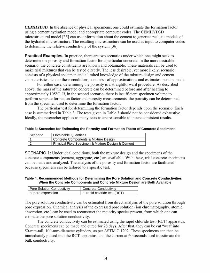
CEMHYD3D. In the absence of physical specimens, one could estimate the formation factor using a cement hydration model and appropriate computer codes. The CEMHYD3D microstructural model [35] can use information about the cement to generate realistic models of the hydrated microstructure. The resulting microstructure can be used as input to computer codes to determine the relative conductivity of the system [36]. Practical Examples. In practice, there are two scenarios under which one might seek to determine the porosity and formation factor for a particular concrete. In the more desirable scenario, the concrete constituents are known and obtainable. These materials can be used to make trial mixtures that can be tested directly. The less desirable, yet more likely, scenario consists of a physical specimen and a limited knowledge of the mixture design and cement characteristics. Under these conditions, a number of approximations and estimates must be made.

For either case, determining the porosity is a straightforward procedure. As described above, the mass of the saturated concrete can be determined before and after heating to approximately 105°C. If, in the second scenario, there is insufficient specimen volume to perform separate formation factor and porosity measurements, the porosity can be determined from the specimen used to determine the formation factor.

The particular test for determining the formation factor depends upon the scenario. Each case is summarized in Table 3. The tests given in Table 3 should not be considered exhaustive. Ideally, the researcher applies as many tests as are reasonable to insure consistent results. Table 3: Scenarios for Estimating the Porosity and Formation Factor of Concrete Specimens

Scenario Obtainable Quantities 1 Concrete Components & Mixture Design 2 Physical Field Specimen & Mixture Design & Cement

SCENARIO 1: Under ideal conditions, both the mixture design and the specimens of the concrete components (cement, aggregate, etc.) are available. With these, trial concrete specimens can be made and analyzed. The analysis of the porosity and formation factor are facilitated because specimens can be tailored to a specific test. Table 4: Recommended Methods for Determining the Pore Solution and Concrete Conductivities

When the Concrete Components and Concrete Mixture Design are Both Available

Pore Solution Conductivity Concrete Conductivity a. pore expression a. rapid chloride test (RCT)

The pore solution conductivity can be estimated from direct analysis of the pore solution through pore expression. Chemical analysis of the expressed pore solution (ion chromatography, atomic absorption, etc.) can be used to reconstruct the majority species present, from which one can estimate the pore solution conductivity.

The concrete conductivity can be estimated using the rapid chloride test (RCT) apparatus. Concrete specimens can be made and cured for 28 days. After that, they can be cut “wet” into 50-mm-tall, 100-mm-diameter cylinders, as per ASTM C 1202. These specimens can then be immediately placed into the RCT apparatus, and the current at 60 seconds used to estimate the bulk conductivity.

15

SCENARIO 2: Given only a field specimen and limited information about either the mixture design or the cement characteristics, there are still a number of procedures that can be applied, as shown in Table 5 below. The most useful of these tests can be applied to the specimen without any additional information. Table 5: Recommended Methods for Determining the Pore Solution and Concrete Conductivities

When a Physical Field Specimen and the Concrete Mixture Design are Both Available

Pore Solution Conductivity Concrete Conductivity a. pore expression a. rapid chloride test (RCT) b. Taylor model b. impedance spectroscopy

The best approach for estimating the formation factor consists of saturating the specimen

and making direct measurements. If available, information about the mixture design and cement characteristics can be used to estimate the composition of the pore solution. This estimation can be made using either the Taylor model or CEMHYD3D. This estimation does not have to be accurate, only reasonable. The specimen can then be vacuum saturated with this estimated pore solution and allowed to equilibrate while submerged within the solution.

The rapid chloride test apparatus can be used to estimate the specimen conductivity by filling the end chambers with the saturation solution. This way, the specimens can be returned to the saturation condition and the conductivity measurement repeated at a later time. This process can be repeated until the conductivity does not change, indicating the specimen has come to equilibrium. Although more precise, impedance spectroscopy is listed second because it requires more expensive equipment, but does not necessarily yield better results.

After the bulk specimen conductivity has been determined, the pore solution conductivity can be determined from either estimation or direct measurement. An estimate can be based on the composition of the saturation solution and knowledge of the duration of saturation required to achieve a constant bulk conductivity measurement. Otherwise, the pore solution can be analyzed from specimens obtained by pore expression. Absorption In the previous section, the diffusion of ions into a fully saturated concrete was discussed. In this section, penetration of sulfate into a dry or only partially saturated concrete specimen will be examined. The sulfate will then diffuse through the structure and react with the cement paste hydration products. Therefore, a test needed to be developed to measure the rate of ingress of water in a concrete specimen. There are two approaches: 1) in-situ testing, i.e., the concrete is tested in place in the field; 2) laboratory testing, i.e., concrete cores are taken and brought to a laboratory for testing. Both approaches have their advantages and disadvantages. In the in-situ approach, the concrete cannot be conditioned and it is impossible to know the water content of the concrete. In the laboratory approach, the concrete might not be exactly the “same” as the in-situ concrete, i.e., curing, hydration degree, etc., if, for example, substantial time elapses between obtaining the cores and testing them. On the other hand, in the laboratory, the concrete can be conditioned and therefore the water content can be known.

The approach selected here is laboratory testing because it was felt that a higher reliability could be achieved, as sorptivity is highly dependent on saturation. The data provide a good estimate of the material properties that can then be used to model the performance of the

16

in-situ concrete as a function of the environment. The test described here was approved as an ASTM standard in 2004 as C 1585: “Standard Test Method for Measurement of Rate of Absorption of Water by Hydraulic-Cement Concretes.” Preconditioning of the specimen. The absorption of water by a concrete specimen depends heavily on its degree of saturation. A fully-saturated specimen will not absorb water, while a fully-dried specimen will absorb a lot. Therefore, the measurements should be conducted on specimens that have the same degree of saturation. NIST developed a method to precondition all specimens to the same level of saturation in equilibrium with approximately 60% RH. To develop the procedure several tests were done and are described in Reference [37]. Here, only the description of the final procedure will be given.

As the sorptivity depends on the water saturation of the concrete, the conditioning of the specimen is paramount. Therefore, the requisite for consistent, uniform conditioning of the specimen should be:

• Equilibrium with the same relative humidity should be achieved with any concrete • The relative humidity in equilibrium with the specimen should be around 60%, because it

is a likely limit on the lowest relative humidity encountered in the field • The duration of the conditioning should be as short as possible • The methodology should not require sophisticated instrumentation. This will allow the

implementation of the test by most laboratories

Therefore, the more severe conditioning consisting of drying the specimen to constant mass in an oven was rejected a priori. On average, a concrete specimen 100 mm in diameter and 50 mm long will need 2 to 3 months to be completely oven dried at a temperature of 50°C. This duration is not acceptable. Drying at higher temperatures might accelerate the evaporation of the water but it could also induce cracking that would alter the sorption coefficient of the specimens. The methodology adopted to determine the optimum conditioning was:

• Phase I: Place the specimens in an environmental chamber at 80% RH and 50°C. The duration of this treatment should be the shortest possible to obtain the same equilibrium RH with all concretes.

• Phase II: Place the specimen in a closed container at 20°C until the specimen has the same RH throughout its thickness. It was determined that all specimens will reach equilibrium after 15 days.

The selection of the duration of the conditioning and the temperatures were determined by

several tests described in Ref. [37]. Duration of exposure to phase I was determined by measuring the scatter of the equilibrium RH reached with various concretes after treatment duration varying from 1 day to a condition of constant mass (several months). Figure 2 shows the results obtained. The RH is measured by placing the specimen in a closed container and measuring the RH in that container. Initially, the RH increases rapidly and eventually it reaches equilibrum. It is assumed that at this point the water content in the specimen is uniformly distributed throughout the specimen. From Figure 2, it is clear that the conditioning from T3 and higher are acceptable, with a small unexplained exception of T4 (3 days). Therefore, we suggest that the specimens should be kept in the environmental chamber for at least 48 hours prior to placement in the container to equilibrate the RH. Of course the smallest variation between

17

specimens is obtained when constant mass is achieved but the duration of the conditioning is not acceptable for a standard test (T7).

30

40

50

60

70

80

90

T1 T2 T3 T4 T5 T6 T7

Type of Preconditioning

RH

[%]

Figure 2 [37]: Relative humidity achieved after the various preconditionings. The main difference is the time spent in the environmental chamber at 50°C and 80% RH. T1: no time; T2: 24 hours; T3: 48 hours; T4: 3 days; T5: 7 days; T6: until constant mass; T7: until constant mass at 20°C and 80% RH. The error bars represent one standard deviation.

The duration required for a specimen to reach equilibrium after conditioning at 50°C and 80% RH, i.e., even distribution of the water throughout the specimen, needs to be determined. To determine the shortest duration needed, specimens were placed in special containers [37]. The RH inside the containers was monitored once a day for up to 30 days. Figure 3 shows the evolution of the RH versus time for some representative specimens. It can be deduced that after about 10 days the RH does not change significantly. Therefore, the duration adopted of 15 days should guarantee a uniform RH throughout the specimen.

Figure 3 [37]: RH of the air inside the conditioning containers versus time. Each curve represents measurements on a concrete cylinder. Each point is the average of data on three slices of a concrete cylinder. The error bars represent one standard deviation.

30

40

50

60

70

80

0 10 20 30Time [d]

RH

[%

]

18

Water ingress into a nonsaturated concrete structure is due to sorption, driven by capillary forces [38]. If the water is on top of the concrete surface, gravity also will play a role in the water penetration. Figure 4 shows the different results obtained with the two methods: capillary rise (water at the bottom of the specimen) or ponding (water at the top of the specimen). It is clear that the specimens have a higher water intake by ponding than by capillary transport. Therefore, it is necessary to use the method that is more appropriate for the concrete structure to be evaluated. The sorptivity coefficients are 0.49⋅10-3 m⋅s-½ for the capillary sorption method and 0.59⋅10-3 m⋅s-½ for the ponding sorption method in this example. Test method description. The method is similar to that recently published as a RILEM recommendation [39]. The principle of the method is that a concrete specimen has one surface in contact with water while the other surfaces are sealed.

The proposed standard test allows either the top surface to be in contact (simulation of water on a pavement or bridge deck) or the bottom surface (substrate in contact with water). The first case is referred to as absorption by ponding and the second as absorption by capillary rise. ASTM C 1585 allows only absorption by capillary rise because the ASTM committee thought that two methods of exposing the specimen to water was too confusing. The concrete specimens were 50-mm-(2-in.)-thick disks sliced from the received specimens. The sides were covered with impermeable adhesive sheet such as duct tape, while the bottom (nontested side) was protected during testing with a plastic sheet loosely attached to the specimen. In the case of absorption by capillary rise (Figure 5) the specimen was then ready for testing. For testing with absorption by ponding, some duct tape was used to form a pond as shown in Figure 6. A two-component epoxy caulk was used to seal the space between the tape and the concrete.

19

Figure 4: Comparison of sorption measured by capillary and by ponding. A) The water content per surface area versus linear time as measured, B) the water content per surface area versus square root of time for the first 7 hours. These are results for one sample and no uncertainty was calculated as they are given only as an example of results that could be obtained.

The mass of the specimen was regularly measured after the tested surface was patted dry. Of course, in the case of ponding, the water inside the dike needed to be poured out before patting dry the specimen surface.

0.00

0.10

0.20

0.30

0.40

0.50

0.60

0 1 2 3 4 5

Time [d]

Mas

s/su

rfac

e[m

]

CapillaryPonding

A

0.00

0.04

0.08

0.12

0.16

0.20

0 50 100 150

Time [s1/2]

Mas

s/su

rfac

e[m

]

Capillaryponding

B

20

Figure 5: Schematic of capillary sorption test.

Figure 6: Schematic of ponding sorption test.

Sealing Material

(15

±5)

mm

(6 ±

1) m

mTape

(100 ± 6) mm

(50

±3)

mm

Caulk < 5 mm

Specimen

Water

Plastic bag or sheet

Sealing Material

(15

±5)

mm

(6 ±

1) m

mTape

(100 ± 6) mm

(50

±3)

mm

Caulk < 5 mm

Specimen

Water

Plastic bag or sheet

21

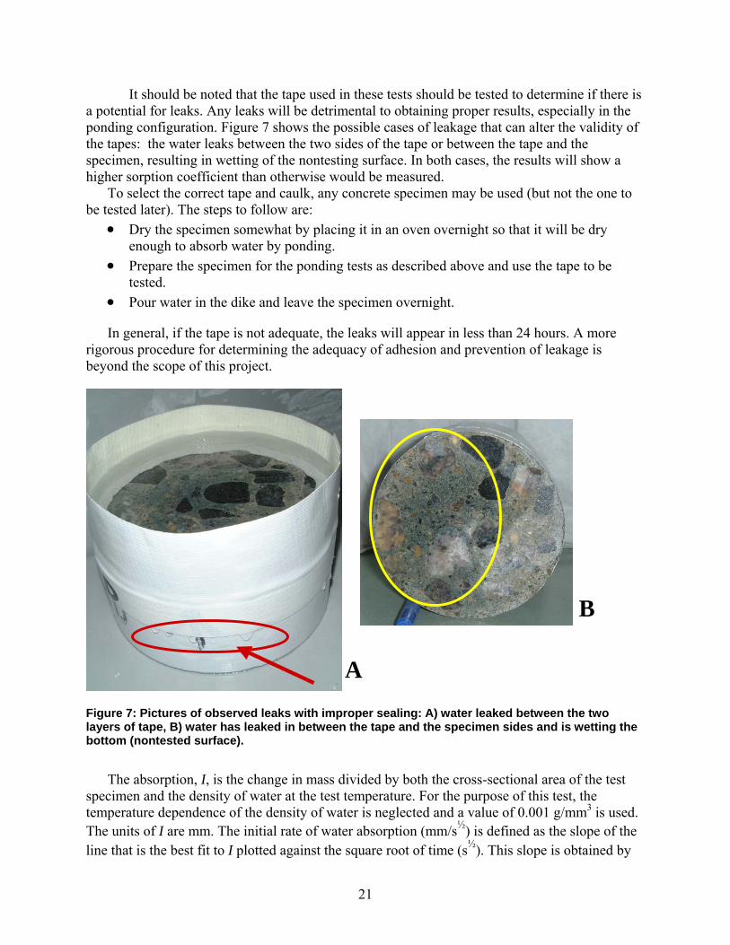
It should be noted that the tape used in these tests should be tested to determine if there is a potential for leaks. Any leaks will be detrimental to obtaining proper results, especially in the ponding configuration. Figure 7 shows the possible cases of leakage that can alter the validity of the tapes: the water leaks between the two sides of the tape or between the tape and the specimen, resulting in wetting of the nontesting surface. In both cases, the results will show a higher sorption coefficient than otherwise would be measured.

To select the correct tape and caulk, any concrete specimen may be used (but not the one to be tested later). The steps to follow are:

• Dry the specimen somewhat by placing it in an oven overnight so that it will be dry enough to absorb water by ponding.

• Prepare the specimen for the ponding tests as described above and use the tape to be tested.

• Pour water in the dike and leave the specimen overnight.

In general, if the tape is not adequate, the leaks will appear in less than 24 hours. A more rigorous procedure for determining the adequacy of adhesion and prevention of leakage is beyond the scope of this project.

A

B

Figure 7: Pictures of observed leaks with improper sealing: A) water leaked between the two layers of tape, B) water has leaked in between the tape and the specimen sides and is wetting the bottom (nontested surface).

The absorption, I, is the change in mass divided by both the cross-sectional area of the test specimen and the density of water at the test temperature. For the purpose of this test, the temperature dependence of the density of water is neglected and a value of 0.001 g/mm3 is used. The units of I are mm. The initial rate of water absorption (mm/s½) is defined as the slope of the line that is the best fit to I plotted against the square root of time (s½). This slope is obtained by

22

using least-squares, linear regression analysis of the plot of I vs. time½. For the regression analysis, all the points from 1 minute to 6 hours or until the plot shows a clear change of slope (Nick point time [see Figure 8]) are used.

The later-age rate of water absorption (mm/s½) is defined as the slope of the line that is the best fit to I plotted against the square root of time (s½) using all the points from 1 to 7 days. Again the least-square linear regression is used to determine the slope. Figure 8 shows these two slopes or sorption coefficients. Two slopes have been observed for the results obtained from a wide variety of concretes and mortars [40]. The later-age sorption coefficient is usually attributed to other phenomena besides the capillary forces alone, such as filling of the larger pores and air voids.

Figure 8: Calculation of the sorption coefficient.

Status. This test was submitted to ASTM and approved in 2003 with inclusion in the ASTM Vol. 04.02 in 2004. The committee used only absorption by capillary rise for inclusion in the procedure. A precision statement is being developed by the ASTM committee, which is conducting a round-robin. This test was developed with the collaboration of Doug Hooton of the University of Toronto, who is also the chair of the ASTM committee. Wet-dry Cycles In the previous two sections, we examined the penetration of sulfate into a concrete that was either immersed or partially saturated. Now, the case of cycles between immersion and exposure to air (drying conditions) needs to be examined. In the field, it is not unusual to have a structure that is not constantly immersed or is only partially immersed in a sulfate solution. For instance, on pier columns, the portion totally and constantly immersed in the water is observed not to deteriorate while the portion in the tidal zone is completely destroyed [41]. It is essential to

0.00

0.05

0.10

0.15

0.20

0.25

0.30

0 200 400 600 800 1000

Time [s1/2]

Mas

s/su

rfac

e [1

0-3 m

]

Early age

Later age

Nick point time

23

determine the mechanisms of deterioration in this case to be able to predict the sulfate resistance of a concrete subjected to wet-dry cycles or partial immersion.

After an overview of the possible mechanisms, a new test method to measure the deterioration on concrete or mortar is presented. Some preliminary results of the tests will also be presented. Some ideas and suggestions for further research will also be discussed. Background. Since concrete is a porous material, the ingress of water is rarely completely prevented. Temperature cycles in combination with the presence of water and salts are the prerequisite for several deterioration mechanisms: freezing and thawing of water, chemical attack, crystallization pressure, and thermal stresses. In this report, the interest is in a concrete structure under external sulfate attack and with temperature and wet/dry cycles, or partially immersed. In the case where only thermal cycles are present in saturated or partially saturated specimens, the potential deterioration mechanisms are varied [42]: 1) stresses due to the expansion of the water during freezing (for temperatures below the freezing point); 2) mismatch of coefficients of thermal expansion between the various components of the concrete, such as the various hydration products or salt precipitated in the pores; or 3) structural changes in salts that might be precipitated in pores. The first phenomenon, freeze-thaw, is well known and will not be addressed in this report. This report concentrates mainly on the last case, with a brief description of Case 2. In the rest of the paper, we assume that the temperature stays above the freezing point of water containing dissolved salts.

If a thermal cycle occurs and the coefficient of thermal expansion (CTE) of the salt and the hydration products is not the same, a few degrees increased temperature could create stresses on the structure [42]. Scherer et al. [42] give the example that a mismatch of CTE of 30 g/t/°C could lead to a stress of 1 MPa per degree change in temperature. Therefore, a small change in temperature between night and day could lead to cracks if the stress generated exceeds the tensile strength of the structure.

It is generally accepted that in the case of wet and dry cycles with exposure to sulfate solution, the pores are filled slowly with salts that precipitate in the pores during the dry cycle. During the wet cycles, the pores are filled with salt crystals and supersaturated solutions (salt concentration higher than the solubility value). The pore size distribution, the type of salt, and the environmental conditions (RH, temperature, and duration of the cycles) are paramount to the type and extent of the deterioration observed.

Depending on the environmental conditions, efflorescence can be observed on the surface of the concrete, or subefflorescence could be formed below the surface. Efflorescence is not aesthetically pleasing, but in some case can be easily eliminated by washing the surface, while the subefflorescence could generate stresses that will deteriorate the structure. The mechanisms of crystal growth inside a structure and the resulting crystallization pressure need to be understood to design concrete that is sulfate resistant.

Crystallization pressure. It is generally agreed [43] that the main cause of spalling under exposure to sulfate solution and wet/dry conditions is due to the crystallization pressure. There are several theories on how the crystallization pressure develops. The best studies on this topic are provided by Scherer [42] and Flatt [43]. A summary of the various theories will be provided here.

A crystal will grow in all directions until its surface attains a local weighted mean curvature [44] that is in equilibrium with the concentration of the solution following the

24

Freundlich equation. Due to large interaction of repulsive forces existing between the crystal and the surface of the pore, the crystal will stop growing toward the pore surface if it is “close” to the surface. Direct contact will not be possible [45] due to the large forces to overcome the surface tension. A thin film of solution forms in the interface of the crystal and the wall of the pore [46, 54]. The concentration of the solution in this thin film should be the same as in the rest of the pore. This concentration is not in equilibrium with the radius of the pore but is in equilibrium with the tip of the crystal free to grow in the area not in contact with the wall. Therefore, as the film will always be supersaturated, the crystal will have a tendency to grow in the direction of the wall, creating a pressure.

In the particular case of sodium sulfate, we need to consider also the structural changes due to a change in RH and/or temperature [47, 48]. Sodium sulfate combined with water has two stable phases: mirabilite (Na2SO4⋅10H2O) and thenardite (Na2SO4), and a metastable phase (Na2SO4⋅7H2O) that is very rare. Magnesium sulfate has three potential phases: epsomite (MgSO4⋅7H2O), hexahydrite (MgSO4⋅6H2O), and kieserite (MgSO4⋅H2O). Some properties of the salts and their crystallization pressures are shown in

Table 6 [48]. In Table 6 the crystallization pressures were computed using Correns’ [46]

equation. The pressure depends on the ratio of bulk solution concentration (C) to the concentration at the crystal solution interface (Cs). The higher ratio occurs when there is a constant evaporation and capillary transport of solution into the concrete. This is exactly the situation in a tidal zone or in wet/dry cycles.

If we assume that the flexural strength of concrete is around 4 MPa, it can be deduced from Table 6 that for sodium and magnesium sulfate, values of C/Cs of 2 will lead to crystallization pressure that could exceed the tensile strength of the concrete. Higher temperature seems to lead to higher pressure.

25

Table 6: Properties of Sodium and Magnesium Sulfate Salts [48]

Crystallization Pressure [MPa] C/Cs = 2 C/Cs = 10 C/Cs = 50

Salt Formula Density [g/cm3]

Molecular weight [g/mol]

Molar Volume [cm3/mol] 0 °C 50°C 0 °C 50 °C 0 °C 50 °C

mirabilite Na2SO4⋅10H2O 1.46 322.19 220 7.2 8.3 23.4 27.7 39.7 47.3

thenardite Na2SO4 2.69 142.04 93 29.2 34.5 97.0 115.0 165.0 196.5

epsomite MgSO4⋅ 7H2O 1.68 246.40 147 10.5 12.5 35.0 41.5 59.5 70.8

hexahydrite MgSO4⋅ 6H2O 1.75 228 130.1 11.8 14.1 39.5 46.9 67.1 30.0

kieserite MgSO4⋅ H2O 2.45 138.39 56.55 27.2 32.4 91.0 107.9 154.3 184.0

C = Solute concentration in bulk solution (supersaturation) [mol/cm3] Cs = Solute concentration at the crystal solution interface [mol/cm3]

26

These data do not take into account the influence of the temperature on the preferential formation of one of the phases of the sodium or magnesium sulfate.

Many authors [43, 49] have observed another phenomenon that occurs with sodium sulfate. This phenomenon is related to the transformation of thernadite to mirabilite by dissolution. Flatt [43] has developed a phase diagram for thernadite and mirabilite as a function of the temperature and RH. He found that above 32.4°C there is no mirabilite. At 25°C, for example, if RH increases above 78%, thernadite is transformed into mirabilite by dissolution and precipitation. A further increase of RH above 82% results in a supersaturated solution of mirabilite. At a RH higher than 92%, a solution of sodium sulfate is present. Flatt showed that a stress of 19 MPa could be calculated from the thernadite dissolution and precipitation to mirabilite. This value is often higher than the tensile strength of concrete. Some authors [50] state that the molar volume of mirabilite is 315% that of thernadite. They infer that the increase of volume is the cause of the crystallization pressure. This would imply that thernadite could absorb water like a sponge to become mirabilite. It should also imply that the specimen should shrink during the drying cycle when mirabilite is transformed back into thernadite. This has not been observed.

A very good picture of what is happening in a tidal zone is shown by Brown [51]. He calculates that depending on the soil saturation and the RH of the air surrounding the wall, a portion of the wall just above the soil level always will be saturated, while at higher levels on the wall evaporation will create favorable conditions for subefflorescence or surface efflorescence.

From the literature survey, it could be summarized that: • Volume change from thernadite to mirabilite could not be the source of the crystallization

pressure. Thernadite does not absorb water molecules to transform into mirabilite. This could be determined by observation that their crystal structures are different. Therefore, the conversion from one to the other is achieved by dissolution and precipitation [54].

• Crystal growth in a pore is a combination of the solution concentration and the size of the pore. A film of supersaturated solution forms between the crystal and the pore wall [42]. This film, which allows the crystal to continue growing toward the wall, is responsible for the crystallization pressure and therefore for the deterioration observed.

• A phase diagram was established for the mirabilite and thernadite versus the temperature and humidity [43]. − Below 32.4°C in temperature, thernadite is formed during the dry cycle and, as the

RH is increased, mirabilite is formed. With a further increase in RH, a supersaturated solution of mirabilite is formed, leading to crystallization pressure in pores. This explains why the deterioration is usually observed in the wet part of the cycle.

− At a temperature above 32.4°C, the decrease in RH precipitates a stable phase of thernadite. Mirabilite is not formed. It would be expected that little or no deterioration would occur [43].

• In a porous material, the pore size distribution will determine the potential for deterioration by crystallization pressure [45]. The pressure is higher in small pores because the interaction between the surface of the pores and the crystal is higher. On the other hand, for the crystal to grow in the small pores, ions need to be transported from the large pores to the smaller ones to maintain the supersaturation of the solution in the small

27

pores. Therefore, the controlling factors for crystallization pressure are the pore size distribution and the average distance between the pores (e.g. spacing factor).

Principle of tests. Ideally, we should be able to measure the pore size distribution of a material and determine the potential for deterioration depending on the environment (RH and temperature). Unfortunately, the correct pore size distribution needed to avoid deterioration has not been determined, and it will be hard to obtain it reliably in concrete. Of course, it could be assumed that if the sorption coefficient [52] would be low enough so that the water and the sulfate solution would not penetrate, there would be no deterioration due to wet/dry cycles. The correlation between the sorption coefficient and the rate of deterioration has not yet been established. Therefore, an empirical test is necessary to determine the susceptibility of a concrete to cyclical sulfate attack.

The objective of designing this test was to be able to determine the concrete mixture that will resist deterioration due to wet-dry cycles or a partial dry-wet environment. Ideally, it should be an accelerated test. A key observation of concrete deterioration is the influence of temperature and RH, which means that the temperature and the RH should be controlled. Therefore, the use of an environmental chamber with controlled temperature and RH was thought to be a necessary component.

The determination of the duration of the wet-dry cycles and the type of measurements to be conducted were the main issues to be solved. As the cycles typically experienced in the field are not always known, with the exception of the tide, it was decided that a stable and controlled temperature and RH were more important than arbitrarily setting the duration of each cycle. The other consideration was to reduce the amount of manipulation needed to perform the test. Therefore, the test will simulate a tidal zone, with a specimen partially immersed in sodium sulfate solution. Experimental setup. As stated above, the experimental setup consists placing a specimen half-immersed in a sulfate solution and exposed to a temperature- and RH-controlled atmosphere. Figure 9 shows a specimen prepared for testing.

The solution penetrates the specimen by capillary sorption or by diffusion, depending on the saturation level of the specimen initially. The total porosity and the pore size distribution will govern the diffusion of the water out of the specimen in the upper part of the specimen (dry zone). This test is inspired by tests conducted on stone by various researchers [53, 54].

To avoid evaporation of the solution, a film of paraffin oil is placed on top of the solution. The specimen is isolated from the paraffin oil by a plexiglas tube inside an expanded polystyrene cylinder. The specimen is placed on spacers glued at the bottom of the container to ensure that the solution can penetrate from the bottom as well. As the experimental setup is placed in an environmental chamber, the temperature and RH could be selected to simulate many environments. It could also be imagined that the temperature and/or the RH could be cycled.

To monitor the specimen deterioration, the top and bottom diameter as well as the height of the spalling above the solution level were measured. In principle, any size specimen could be used provided that the height is at least twice the diameter. The specimen is marked with two circles 19 mm (0.75 in.) from the top and 19 mm (0.75 in.) from the bottom and with 4 vertical lines equally spaced around the perimeter as shown in Figure 10. The width of any deterioration was measured on each vertical line. The average of the width of the deterioration was reported as

28

a measurement of deterioration. Also the top and bottom diameters were monitored as a measurement of expansion.

RH, T

Paraffin oil

None of the surfaces of the specimen are protected

Salt solution

Figure 9: Schematic of the specimen setup for the wet-dry cycles.

100

mm

50 m

m

Water line

19 m

m19

mm

50 mm

Figure 10: Marking of the specimens for measurements.

Results. To determine the validity of this experimental setup, three series of tests were performed. The first set used concrete cores, while the other two used mortar cylinders prepared for this experiment. In the first case, all the measurements described above were not performed because this set was used to determine the best method to monitor the deterioration. The second set was composed of two mortars prepared with the same mixture design but with two different cements: a Type I cement and a blended cement containing silica fume (15% replacement by mass). The blended cement with silica fume was selected because it showed no expansion in the mortar prism tests (see section "Mortar specimens"). In all cases the sodium sulfate solution was prepared as described in ASTM C 1012.

Concrete specimens. Two concrete cores from a road in Maryland (provided by the Maryland Department of Transportation) were used. The cores were 50 mm (2 in.) in diameter and 10 mm

29

(4 in.) long. One specimen was placed at 80% ± 5% RH and the other was placed at 30 % ± 5 % RH. The temperature in both cases was 25°C ± 2°C. Pictures were taken and mass of the specimens measured regularly for 6 months. The mass measurements were not very indicative of the deterioration observed because it is hard to correctly dry the surface of the specimen prior to the measurement without increasing the deterioration by removing some loose material. The visual observations are more indicative of the deterioration.

Figure 11 shows the deterioration seen after 25 weeks of exposure. The following observations can be made:

− The specimen at 80% RH showed signs of deterioration first (42 days instead of 75 days). − The zone of deterioration is very large and starts at the water level for the specimen

exposed to 80% RH. − The zone of deterioration is narrower and is situated at a certain distance from the water

level for the specimen at 30% RH. The first sign of deterioration was a crack and not spalling at about 75 days.

− The first appearance of spalling was at 105 days for the specimen subjected to 30% RH while only at 42 days for the specimen at 80%.

These preliminary results led us to better determine the parameters that should be monitored:

the height “D” (Figure 11) of the deterioration, and the expansion of the specimen at the top and the bottom. These observations were used to develop the test further and were used in the mortar experiments.

Figure 11: Picture of concrete submitted to the wet-dry deterioration after 25 weeks. D = deteriorated zone. The diameter of the specimens is 50 mm (2 in.) and the height is 101 mm (4 in.).

80 % RH 30 % RH

D

D

Water level

80 % RH 30 % RH

D

D

Water level

30

Mortar specimens. Two sets of mortar specimens were prepared. The first set contained two mortar compositions, while the second set contained three types of mortar. Table 8 shows the composition of the specimens. These mixtures were selected because of their different behavior in a full immersion test both in expansion and dynamic modulus of elasticity (see Figure 12). The silica fume mixture did not deteriorate at all even after 1800 days (30 months) of continuous immersion. The exposures selected were of three types as shown in Table 7. This table also shows which type of mortar was submitted to the various conditions. The scope of these tests was to determine if the parameters selected in the preliminary tests would enable us to rank the materials from their relative deterioration. Table 7: Type of Exposure

Environment Specimens Temperature [°C] RH [%] Set # 25 80 1,2 25 30 1,2 40 80 2

Table 8: Composition of the Specimens for Sets #1 and #2

Supplementary Cementitious Material Specimen

W/Cm

S/Cm Name Replacement of

cement [%] by mass Control 0.485 2.75 None 0 SF 0.511* 2.75 Silica Fume 15 FA-C 0.485 2.75 Fly Ash Class C 15

Note: * the w/c ratio was adjusted to obtain a workable mix.

31

A

B Figure 12: Expansion (A) and modulus of elasticity (B) of prisms made with the same composition as shown in Table 8. All data for the expansion are an average of three specimens. The modulus is the average of two specimens. The error bars represent the one standard deviation in both graphs. The expansion of the control is measured with only two specimens after 360 days (The third specimen broke.)

0.00

0.50

1.00

1.50

2.00

2.50

3.00

0 500 1000 1500 2000 2500

Time [d]

Expa

nsio

n [%

]control

FA-C

SF

15

20

25

30

35

40

45

0 200 400 600 800 1000Time [d]

Mod

E [G

Pa]

control

FA-C

SF

32

As a tentative procedure to accelerate the process, the pH was controlled manually for the specimens in set #1. Once a week, when the specimens were measured, the pH was adjusted to maintain a value of 7. As this was done manually, it was hard to add the correct amount; therefore, most of the time the pH was lower than 7. The pH measured before the adjustment was always higher than 7, between 9 and 12. Therefore, there was some acid attack for the portion of the specimen immersed in the solution. This explains why the bottom diameters are decreasing with time instead of expanding. This procedure was abandoned for set #2 and replaced by changing the solution every month.

In both sets, the top and bottom diameter and the width of the spalling were measured weekly. Some pictures were taken to visually monitor the specimens. Figure 13 and 14 show the results obtained for set #1, and Figure 15 to Figure 17 shows the results of set #2.

0

5

10

15

20

25

30

35

70 90 110 130 150 170

Time [d]

Det

erio

ratio

n w

idth

[mm

]

control 30 %Control 80 %SF 30 %SF, 80 %

Figure 13: Deterioration width of the mortar specimens for set #1 at 25°C. The percentages in the legend are the RH used.

33

Figure 14: Relative expansion of the top and bottom diameters for mortar set #1. The percentages in the legend are the RH used.

Figure 15: Deterioration width of the mortar specimens for set #2 at 25°C. There are no data at 40°C because no deterioration was observed. The percentages in the legend are the RH used. The error bars are not shown for clarity but all data would be ± 20% (as seen in Figure 13).

05

1015202530354045

0 100 200 300 400

Time [d]

Wid

th d

eter

iora

tion

[mm

] Control, 30%

FA-C, 30%

SF, 30%

Control, 80%

FA-C, 80%

SF, 80%

control

-3.0

-2.5

-2.0

-1.5

-1.0

-0.5

0.0

0.5

1.0

0 50 100 150

Time [d]

Rel

ativ

e di

amet

ers

[%]

Top 30 %Bottom 30 %Top 80 %Bottom 80 %

SF

-1.8-1.6-1.4-1.2-1.0-0.8-0.6-0.4-0.20.00.2

0 50 100 150

Time [d]

Rel

ativ

e di

amet

ers

[%]

Top 30 %Bottom 30 %Top 80 %Bottom 80 %

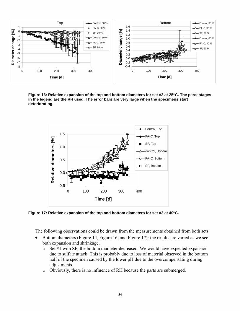
34

Figure 16: Relative expansion of the top and bottom diameters for set #2 at 25°C. The percentages in the legend are the RH used. The error bars are very large when the specimens start deteriorating.

Figure 17: Relative expansion of the top and bottom diameters for set #2 at 40°C.

The following observations could be drawn from the measurements obtained from both sets: • Bottom diameters (Figure 14, Figure 16, and Figure 17): the results are varied as we see

both expansion and shrinkage. o Set #1 with SF, the bottom diameter decreased. We would have expected expansion

due to sulfate attack. This is probably due to loss of material observed in the bottom half of the specimen caused by the lower pH due to the overcompensating during adjustments.

o Obviously, there is no influence of RH because the parts are submerged.

-0.5

0.0

0.5

1.0

1.5

0 100 200 300 400

Time [d]

Rel

ativ

e di

amet

ers

[%]

Control, Top

FA-C, Top

SF, Top

control, Bottom

FA-C, Bottom

SF, Bottom

Top

-8-7-6-5-4-3-2-101

0 100 200 300 400

Time [d]

Dia

met

er c

hang

e [%

]

Control, 30 %

FA-C, 30 %

SF, 30 %

Control, 80 %

FA-C, 80 %

SF, 80 %

Bottom

-0.4-0.20.00.20.40.60.81.01.21.41.6

0 100 200 300 400

Time [d]

Dia

met

er c

hang

e [%

]

Control, 30 %

FA-C, 30 %

SF, 30 %

Control, 80 %

FA-C, 80 %

SF, 80 %

35

o For set #2 expansion is observed for the control and the FA-C cements as expected from the prisms’ length changes measurements.

o For set #2 no expansion is observed for the SF replacement specimen. • The top diameters usually shrink due to evaporation, especially for the low RH. • Table 9 shows the time where spalling was initially observed on the specimen. It seems

that in all cases the spalling starts earlier in the 30% environment than in the 80% and no damage is observed at 40°C. It should be noticed that even the SF specimen starts to deteriorate, while no expansion was measured in prisms. This shows that tidal zone type of exposure is more severe than fully immersion.

Table 9: Initiation of Spalling on the Specimens

Type Init. Det. [d] Set #1 Set #2 Control 25 °C, 30 % 84 41 Control 25 °C, 80 % 163 63 Control 40 °C, 80 % -- >257 SF 25 °C, 30 % 98 40 SF 25 °C, 80 % 129 133 SF 40 °C, 80 % -- >257 FA-C 25 °C, 30 % -- 40 FA-C 25 °C, 80 % -- 103 FA-C 40 °C, 80 % -- >257

To attempt to explain these results, some relevant details are necessary: • The SF specimen is likely to have smaller pores than the control. This could lead to

higher deterioration in this experiment because the solution is carried higher into the specimen by capillary suction, unless the pore network is not percolated.

• In the case of exposure to 80% RH, the specimens experience a range of RH from 100% (close to the solution) to 80% (at the surface or at the top). According to the phase diagram of sodium sulfate vs. RH and temperature [43], this would lead to formation of supersaturated mirabilite solution and no thernadite. It was reported above that this would lead to lower damage because there is no conversion from thernadite to mirabilite.

• In the case of exposure to 30% RH, the specimen experienced a range of RH from 100% to 30%. According to the phase diagram, this would lead to the formation of thernadite and precipitation of supersaturated solution of mirabilite. The damage should be higher due to the higher volume occupied by mirabilite.

• At 40°C the temperature is above the critical point of 32.4°C [43] and therefore no mirabilite is formed. There is no transformation between the two phases, and the crystallization pressure is lower or null because only thernadite can be formed as its volume is smaller.

36

Therefore, in light of the above facts, at temperatures lower than 32.4°C, it is expected that RH of 30% would lead to a higher and more rapid deterioration than exposure to 80%. This observation is confirmed by work performed by Rodriguez-Navarro et al. [54]. They showed that a limestone block exposed to 35% RH was broken in half, while the same block exposed to 60% RH showed only superficial spalling.

The unexpected finding was that the replacement of cement by SF does not prevent deterioration in this type of test, while it did in a complete immersion test. Summary. From the above tests, it can be deduced that if an accelerated test is needed to simulate exposure to wet-dry cycles or in tidal zone conditions, the selection of a low RH and a temperature below 32.4°C is advisable. A RH of 30% is easily achievable at various temperatures using an environmental chamber or a salt solution. The temperature could be selected to reflect the possible environment in the field. It should be kept in mind that if the temperature is consistently above 32.4°C, according to the literature [43] and our preliminary results, this will lead to reduced deterioration.

The measurements selected to monitor the deterioration, i.e., the top and bottom diameters and the width of the spalling, seem to be appropriate. Future Work. So far, we developed a test that could be used both with specimens prepared in the laboratory and cores from the field. This test is semiempirical, but it can quickly show the onset of deterioration due to wet-dry cycles. But this is not a prediction of deterioration from composition.

It is clear that the deterioration depends on the percolation characteristics of the pore structure, the pore size distribution, and the total air content. The pore structure is linked to the capacity of absorption and desorption of water from the specimen. The other important factor is the tensile strength of the cement paste. Therefore, a predictive test based on material science should include the characterization of the pore structure and the tensile strength of the specimen. A link or correlation should be established between the pore structure and the performance under wetting and drying cycles.

After the phenomena are better understood and the important material parameters are determined, it is likely that a model could be developed to predict the deterioration of a mortar or concrete from its physical characteristics. Transport Properties-Based Models To link the concrete characteristics such as formation factor and sorptivity coefficient to the prediction of service life, models are essential. During this project new models were not developed in part because there are three good models that already exist and that are available for free from the NIST website (CONCLIFE, Mobasher-Tixier [55]) or are commercially available (STADIUM2). These models will certainly be further developed in the future and thus improve the prediction capability. 2 Commercial equipment, instruments, and materials mentioned in this paper are identified to foster understanding. Such identification does not imply recommendation or endorsement by the National Institute of Standards and Technology (NIST), nor does it imply that the materials or equipment identified are necessarily the best available for the purpose.

37

NIST CONCLIFE [56]. This model was developed for a project funded by the Federal Highway Administration (FHWA) [37] to address the deterioration by sulfate attack and freeze-thaw of bridge decks and pavements. Regarding sulfate attack, it was assumed that the sulfate solution could ingress the concrete by sorption either from the soil or from rain. This model assumes the following scenarios:

• Sulfates enter only by sorption and not by diffusion. • The concrete specimen is dry or only partially saturated and therefore the solution can

enter by sorption. • As soon as sulfate enters in the concrete it will react with the cement hydration products

and be transformed into ettringite. The composition of the cement is not taken into account.

• Wet-dry cycles are considered by a gradual accumulation of sulfate in the pores of the concrete. As the amount of sulfate increases in the concrete, more ettringite is formed. It is assumed that all the sulfate ions will react with the cement and form ettringite. The crystallization pressure is not taken into account.

The service life model for sulfate attack in CONCLIFE is based on the model developed by

Atkinson and Hearne [57]. While their development considered the main mode of sulfate ion transport into the concrete to be by diffusion, here we will develop a similar model for sulfate ions transported via sorption from the external environment. The basic equation developed by Atkinson and Hearne is [57]: ))(/())1(2( 2

Efspall CEX βναγ −= ( 17 )

where CE = concentration of reacted sulfate as ettringite (mol/m3)

E = Young’s modulus (GPa) Xspall = spalling depth (m) α = roughness factor for fracture path β = linear strain caused by one mole of sulfate reacted (m3/mol) γf = fracture surface energy of concrete (N/m) σ = surface tension (N/m)

ν = Poisson’s ratio (e.g., for concrete, probably close to 0.2, for paste 0.25, and for mortar 0.22)

The basic assumption of this model is that deleterious expansion and cracking are due to

the formation of ettringite within the concrete. When the strain produced by the growing ettringite exceeds the fracture energy of the concrete, failure occurs as a layer Xspall thick spalls from the concrete. For a sorptivity-based model, the buildup of ettringite is considered to be due to external sulfate ions penetrating into the concrete along with the sorbed external solution [58]. Thus, to use this model, the user must specify the concentration of sulfate ions in the external solution (e.g., rainwater or groundwater) and the sorption properties of the concrete. The basic screen within CONCLIFE for performing service life predictions in the case of sulfate attack is shown in Figure 18.

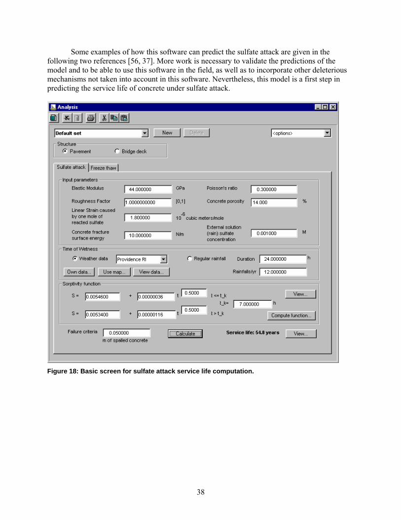
38

Some examples of how this software can predict the sulfate attack are given in the following two references [56, 37]. More work is necessary to validate the predictions of the model and to be able to use this software in the field, as well as to incorporate other deleterious mechanisms not taken into account in this software. Nevertheless, this model is a first step in predicting the service life of concrete under sulfate attack.

Figure 18: Basic screen for sulfate attack service life computation.

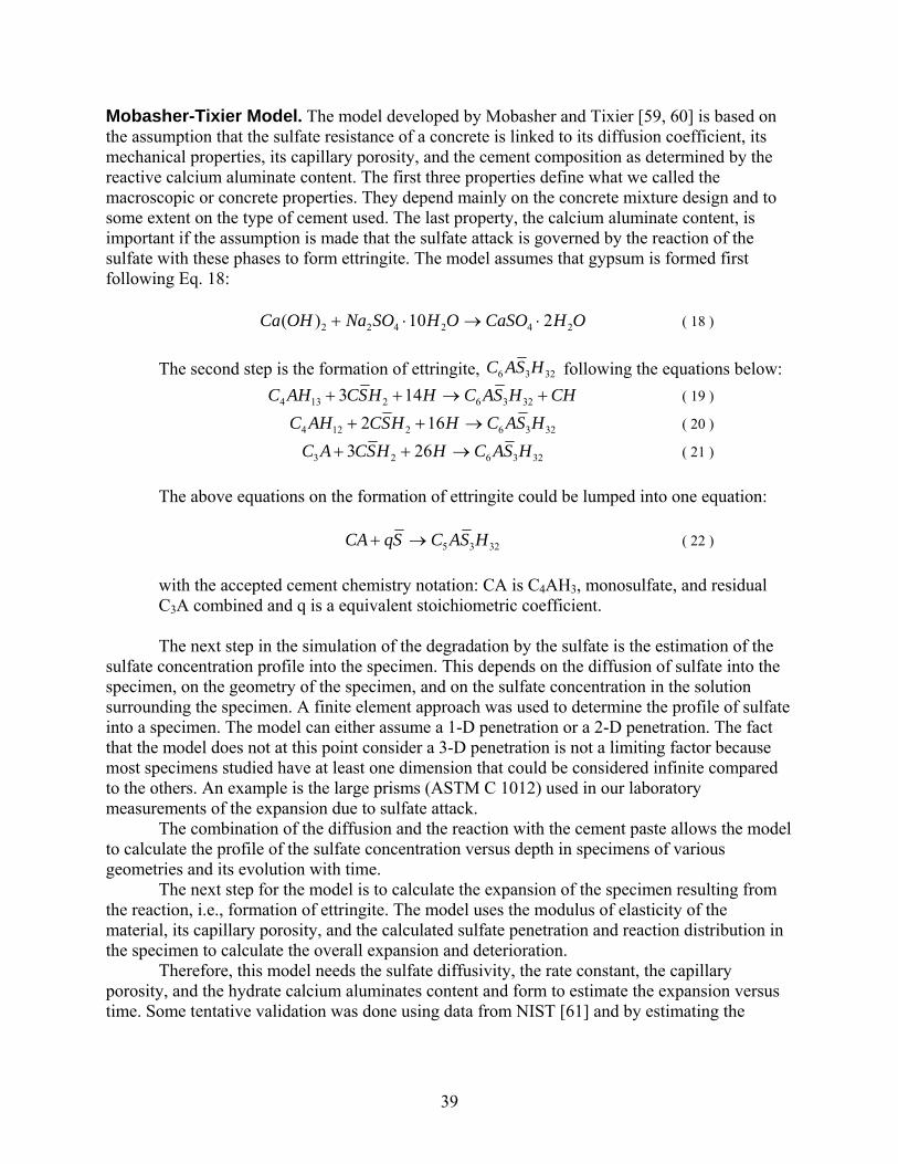
39

Mobasher-Tixier Model. The model developed by Mobasher and Tixier [59, 60] is based on the assumption that the sulfate resistance of a concrete is linked to its diffusion coefficient, its mechanical properties, its capillary porosity, and the cement composition as determined by the reactive calcium aluminate content. The first three properties define what we called the macroscopic or concrete properties. They depend mainly on the concrete mixture design and to some extent on the type of cement used. The last property, the calcium aluminate content, is important if the assumption is made that the sulfate attack is governed by the reaction of the sulfate with these phases to form ettringite. The model assumes that gypsum is formed first following Eq. 18: OHCaSOOHSONaOHCa 242422 210)( ⋅→⋅+ ( 18 )

The second step is the formation of ettringite, 3236 HSAC following the equations below: CHHSACHHSCAHC +→++ 32362134 143 ( 19 )

32362124 162 HSACHHSCAHC →++ ( 20 )

323623 263 HSACHHSCAC →++ ( 21 )

The above equations on the formation of ettringite could be lumped into one equation:

3235 HSACSqCA →+ ( 22 )

with the accepted cement chemistry notation: CA is C4AH3, monosulfate, and residual C3A combined and q is a equivalent stoichiometric coefficient.

The next step in the simulation of the degradation by the sulfate is the estimation of the

sulfate concentration profile into the specimen. This depends on the diffusion of sulfate into the specimen, on the geometry of the specimen, and on the sulfate concentration in the solution surrounding the specimen. A finite element approach was used to determine the profile of sulfate into a specimen. The model can either assume a 1-D penetration or a 2-D penetration. The fact that the model does not at this point consider a 3-D penetration is not a limiting factor because most specimens studied have at least one dimension that could be considered infinite compared to the others. An example is the large prisms (ASTM C 1012) used in our laboratory measurements of the expansion due to sulfate attack.

The combination of the diffusion and the reaction with the cement paste allows the model to calculate the profile of the sulfate concentration versus depth in specimens of various geometries and its evolution with time.

The next step for the model is to calculate the expansion of the specimen resulting from the reaction, i.e., formation of ettringite. The model uses the modulus of elasticity of the material, its capillary porosity, and the calculated sulfate penetration and reaction distribution in the specimen to calculate the overall expansion and deterioration.

Therefore, this model needs the sulfate diffusivity, the rate constant, the capillary porosity, and the hydrate calcium aluminates content and form to estimate the expansion versus time. Some tentative validation was done using data from NIST [61] and by estimating the

40

modulus and other values that were not measured. The agreement with the experiment was very reasonable.

Some collaboration was initiated with Dr. Mobasher to further exploit the data generated by this report to validate his model [62]. Also, the model is available on the NIST website. STADIUM. This finite element model was developed by Marchand [7]. It is based on the principle that all chemically induced alterations induce a change in porosity that will affect the transport properties. To simulate ionic transport, the Nernst-Planck equation, the chemical activity coefficient, and the electrical potential are used. As input to the model, the following parameters are needed: porosity, concentration of species, water content of the concrete, diffusion coefficient, and tortuosity of the pore system. The chemical reactions are treated as a local equilibrium of dissolution and precipitation. The local chemical reaction changes the pore system and therefore affects the transport properties.

The model solves a system of equations that describe: • Transport properties: diffusion coefficient • Chemical reaction • Porosity changes due to the chemical reaction

This model might be commercially available in the near future. Collaboration with the author

is possible, but due to the commercial nature of the product, it would be hard to assume that a combination with the above models would be possible. Summary of the models. In conclusion, there are three models that are in an advanced stage of development. Two of them are available to NIST and to the public, and one will be commercially available.

There are some differences in applications between the models. The NIST CONCLIFE model assumes that the specimen is exposed to the sulfate solution only on one side and allows for cycles of wet and dry surfaces. The Mobasher-Tixier model assumes that the specimen is fully saturated and therefore that the sulfate penetrates by diffusion and not by sorption. They both assume that the formation of ettringite is the cause of the expansion and neither takes into account deterioration by crystallization pressure. CONCLIFE estimates the spalling due to the deterioration while the Mobasher-Tixier model calculates the expansion versus time. These models are complementary. It seems that both models might benefit from a better knowledge of the microstructure evolution during the deterioration. It would be ideal if they could be combined.

STADIUM also attempts to determine the distribution of sulfate throughout the specimen, but it does not seem to attempt to predict the onset of deterioration.

NIST also plans to have a continuation project based on the CEM3HYD [35] program to simulate a virtual deterioration of a cement from its SEM image. The data collected under this project will be used to validate the results of the model. The goal is to be able to predict the resistance to sulfate of a cement based only on the composition as determined from an SEM analysis. Obviously, the prediction of a concrete resistance to sulfate attack should combine the chemistry of the cement resistance with physical properties such as sorption, diffusion, and cyclic loads. No all-in-one model exists at this time, but the scheme proposed here provides all the necessary methods to estimate the resistance of a concrete (Figure 1).

41

CEMENT CHARACTERISTICS Introduction This part of the report addresses the influence of the cement on the sulfate resistance of a structure (right branch of the chart in Figure 1). To predict the sulfate resistance of a cement, a full understanding of the chemical reaction of the hydration product with sulfate is needed. Therefore, two cements and nine supplementary cementitious materials were selected, tests were conducted, and the products from the sulfate interaction with the hydration products were examined, including both microstructure features and macroscopic characteristics such as expansion and modulus of elasticity.

The microstructure observations will be useful as the basis for better understanding the mechanisms and the reaction products developed during a sulfate attack. Once the understanding is more complete, it will be possible to modify a virtual “hydration model,” such as the NIST CEM3HYD model [35] to simulate this reaction, or to develop other models such as a statistical model based on mineralogy and particle size distribution (PSD). The ultimate goal will be to use a SEM/X-ray analysis of a cement paste to produce an image of the cement paste and then determine the phase amounts and spatial distribution in the cement paste. This image can be virtually exposed to a sulfate solution. The model will show the reaction products and their rate of formation. This result will allow the determination of whether the cement examined is sulfate resistant or not in less than a day. The model could also allow the optimization of the cement composition depending on the material available and on the application. This knowledge could lead to the engineering of sulfate resistant cements by selecting the raw materials and the production procedure. For microstructural observations, cement paste and mortar specimens were exposed to sulfate solution. The initial compressive strength was measured but it is clearly not a good indicator of deterioration versus time. The reason is that it is a destructive method and therefore the number of specimens needed is too large to be feasible. The flexural test performed on small bars (25.4×25.4×285 mm or 1×1×11.25 in.) is plagued by such a large scatter of the data that it is unusable. Therefore, two properties were used to monitor the deterioration of the specimens: expansion and dynamic modulus of elasticity. The collection of expansion data along with SEM and XRD examination of specimen sections allowed the construction of a more detailed picture of the kinetics of the reaction than previously attempted [2]. This approach will serve as an input in the future to develop models for prediction of the resistance to sulfate attack from the composition. In the process of acquiring a better understanding of the chemistry and microstructure development, it was discovered that a reduction in size of the prisms from the standard 25×25×285 mm to 10×10×40 mm was justified. This discovery resulted in the development of shorter test periods using only cement paste small specimens.

This section will be divided in three parts: 1. Tests performed to acquire information on the deterioration kinetic 2. Microstructure observation (left branch of the “Cement Characteristics” branch in Figure 1) 3. New test using small specimens (right branch of the “Cement Characteristics” branch in

Figure 1)

42

Tests Performed Materials used. The materials were provided by the PCA and included two cements classified as ASTM Type I/II and Type V and supplementary cementitious materials.

The two cements’ chemical composition is shown in Figure 19 and in Table 10. Table 11 shows the compositional estimates. The phase composition was calculated using the ASTM C 150 method (Bogue calculation) and by X-ray powder diffraction. XRD data represent averaged values from bulk and salicyclic acid/methanol extraction residues. XRD results indicate that the aluminate content of these cements is similar.

The types of supplementary cementitious materials (SCM) used are shown in Table 12. The dosages were initially set to be 1% by mass of cement replacement for all SCM. But it was established that the metakaolin and shale types are effective to prevent sulfate attack only at dosages of at least of 20% to 25%3. As the purpose of this test is to determine the influence of these supplementary cementitious materials on the sulfate attack resistance and not to determine the best dosage for each material, a constant dosage of 1% was selected for all material except for the metakaolin and shale types, whose dosage was set to 25% to better reflect the usual dosage in the field.

3 Private communication with Greg Barger, Ash Grove Cement Co.

43

Figure 19: XRD patterns from a bulk and salicyclic acid-methanol extraction residue for cement Type I/II cement (NIST Code #PCA-12). (Y-axis is densities intensity, X-axis represents degrees 2-theta for Cu Kα radiation.)

44

Figure 20: XRD patterns for bulk (upper) and salicyclic acid-methanol extraction residue for cement Type V (NIST Code # PCA-16). (Y-axis is densities intensity, X-axis represents degrees 2-theta for Cu Kα radiation.)

45

Table 10: Cement Oxide Compositions

Type I/II PCA-12

Type V PCA-16

Na2O 0.156 0.11 MgO 4.21 2.19 Al2O3 4.39 3.97 SiO2 20.4 21.99 P2O5 0.081 0.17 SO3 2.76 2.11 Cl 0.010 <0.002 K2O 0.48 0.70 CaO 63.6 63.95 TiO2 0.440 0.24 V2O5 0.01 0.01 Cr2O3 0.02 0.01 Mn2O3 0.09 0.06 Fe2O3 2.64 3.91 NiO 0.01 0.00 ZnO 0.04 0.03 SrO 0.04 0.08 ZrO2 0.02 0.02 BaO 0.07 0.02 LOI

0.53

0.30

Table 11: Compositional Estimates

Type I/II Type V ASTM

C 150 XRD ASTM

C 150 XRD

Alite 62.5 62.1 54.9 58.9 Belite 11.4 12.1 21.6 14.4 Aluminate 7.2 4.5 3.9 4.9 Ferrite 8.0 9.7 11.9 14.6 Arcanite 0.4 0.3 Periclase 2.3 0.6 Gypsum 0.7 0.4 Bassanite 3.1 3.6 Anhydrite 0.3 0.2 Dolomite 0.8 -- Calcite 0.5 -- Quartz 0.2 0.4

46

Table 12: Supplementary Cementitious Materials Used

NIST Code Type PCA-31A Fly Ash Class F PCA-31B Fly Ash Class C PCA-32A Calcined Montmorillonite Shale PCA-32B Calcined Kaolin (Metakaolin) PCA-32C Calcined Kaolin/Opal PCA-144A GGBFS; Grancem 80 PCA-144B GGBFS; Grancem 120 PCA-144C GGBFS; Grancem 100 PCA-145 Silica Fume

Note: The NIST codes are shown for identification purpose only. (Appendix A provides composition data.)

Specimens prepared. Two sets of specimens were prepared using these materials:

• Set #1: cement paste with the two cements • Set #2: mortars with the two cements and the SCM

The mixture compositions were divided in two sets: cement paste and mortars. Table 13

shows the mixture composition. • Set #1: cement paste water-cement ratio = 0.35 or 0.45 • Set #2: mortar water/cement ratio = 0.485; sand-cement ratio = 2.75 and for some mixes

cement was partially replaced by mass with a SCM

The cement and the SCM were blended in the correct proportion in a V-blender before using to prepare the specimens. Only Type I/II cement was used in these specimens.

Three type of solutions were prepared: • Sodium sulfate: 50 g/L (as described in ASTM C 1012) • Magnesium sulfate: 42.4 g/L. This amount corresponds to the same concentration of

SO4++ as in the sodium sulfate solution

• Limewater: saturated solution of Ca(OH)2

All specimens were cured for 24 hours in 100% RH and 20°C ± 3°C after mixing. All specimens were exposed to the selected solution immediately after demolding (curing method A). After almost a year in limewater, some specimens (see Table 13) were then exposed to sodium sulfate solution (curing method B). This second curing method will show the influence of curing on the sulfate resistance.

The specimens from set #1 were exposed, after curing method A, to sodium sulfate and magnesium sulfate solution as well as limewater. The specimens from set #2 were exposed to sodium sulfate solution and limewater. Some specimens from set #2 were exposed to sodium sulfate after curing method B.

47

For all sets the following specimens were prepared: • Prisms: (25.4×25.4×285 mm or 1 ×1×11.25 in.) used to monitor expansion and dynamic

modulus of elasticity (ASTM C 215) • Small cylinders (25.4 mm [1 in.] diameter and 25.4 mm [1 in.] long) used for SEM and X-ray

diffraction analysis • Cubes (50 mm or 2 in.) used to measure the compressive strength at 7 days and 28 days

The prisms used for expansion had pins (as described in ASTM C 1012) placed at both ends to be used with a comparator, while the prisms used for the modulus of elasticity did not have pins. The small cylinders were used to monitor microstructure evolution during sulfate penetration into the specimens. The small cylinders were coated at both ends with a two-component epoxy so that the sulfate would penetrate the cylinders from the sides only.

In order to compare our methodology with the standard test method (ASTM C 1012), an independent laboratory conducted the measurements on the same materials. Prisms as described in the standard were prepared using the same cement combination as discussed above for the specimens prepared by NIST. Table 13: Specimens Prepared

NIST code Set # W/C SCM Name

Cement type

Curing

PCA-25 1 0.350 None I A PCA-26 1 0.350 None V A PCA-152 1 0.450 None I A PCA-174 2 0.485 None I A,B PCA-175 2 0.485 Fly Ash F I A,B PCA-180 2 0.485 Fly Ash C I A,B PCA-191 2 0.485 Metakaolin I A,B PCA2-12 2 0.485 Calcined Montmorillonite

(Shale) I A,B

PCA2-13 2 0.485 Calcined Kaolin/Opal I A,B PCA2-24 2 0.485 GGBFS 80 I A,B PCA-193 2 0.485 GGBFS 100 I A,B* PCA2-23 2 0.485 GGBFS 120 I A,B PCA2-28 2 0.485 Silica Fume I A,B

*Only prisms for measuring the modulus were available for curing method B

Measurements on mortar prisms. The set #1 results are shown in Figure 21 and Figure 22. The first figure shows the expansion results and the second figure shows the dynamic modulus of elasticity. There are two figures for expansion to be able to show more clearly the expansion of the specimens prepared with the Type V cement. To discuss the results obtained, it should be kept in mind that these are cement paste specimens that were prepared with two cements, at two

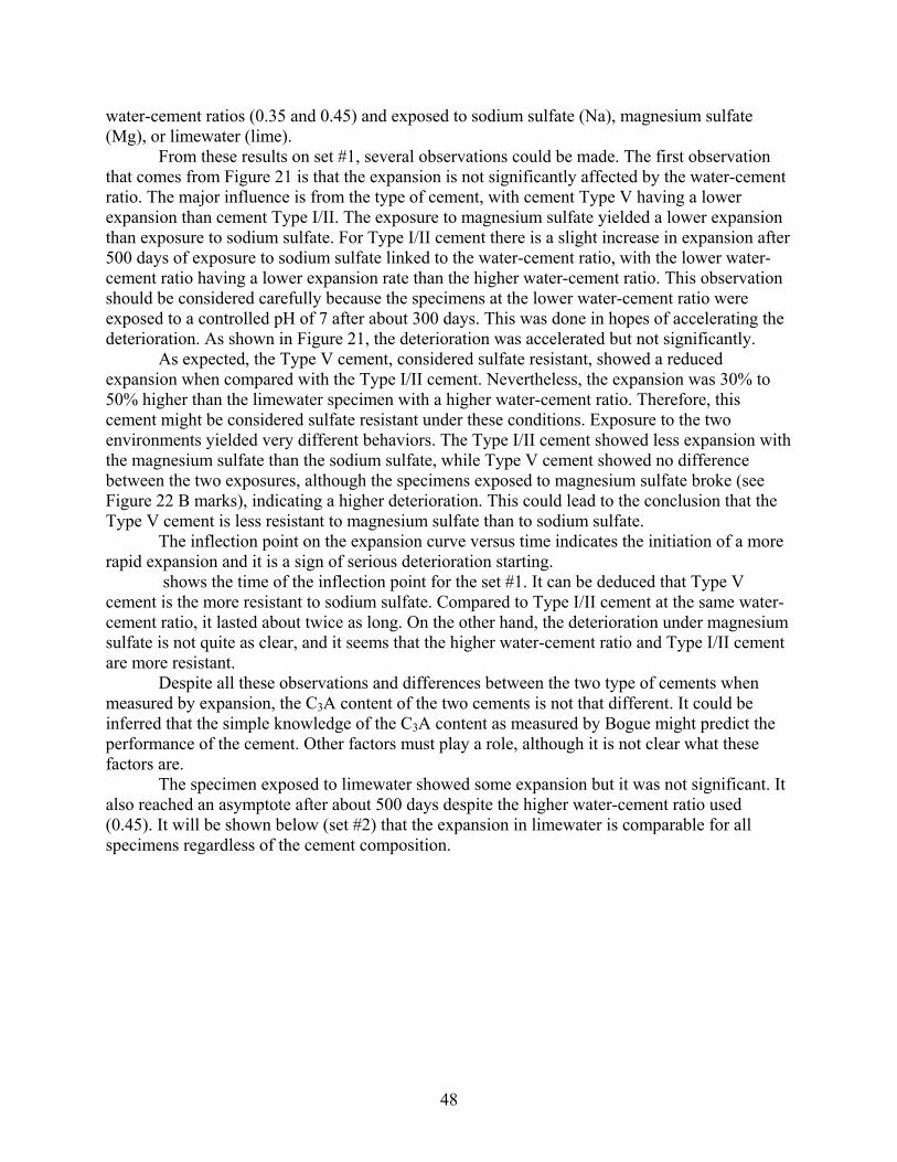
48

water-cement ratios (0.35 and 0.45) and exposed to sodium sulfate (Na), magnesium sulfate (Mg), or limewater (lime).

From these results on set #1, several observations could be made. The first observation that comes from Figure 21 is that the expansion is not significantly affected by the water-cement ratio. The major influence is from the type of cement, with cement Type V having a lower expansion than cement Type I/II. The exposure to magnesium sulfate yielded a lower expansion than exposure to sodium sulfate. For Type I/II cement there is a slight increase in expansion after 500 days of exposure to sodium sulfate linked to the water-cement ratio, with the lower water-cement ratio having a lower expansion rate than the higher water-cement ratio. This observation should be considered carefully because the specimens at the lower water-cement ratio were exposed to a controlled pH of 7 after about 300 days. This was done in hopes of accelerating the deterioration. As shown in Figure 21, the deterioration was accelerated but not significantly.

As expected, the Type V cement, considered sulfate resistant, showed a reduced expansion when compared with the Type I/II cement. Nevertheless, the expansion was 30% to 50% higher than the limewater specimen with a higher water-cement ratio. Therefore, this cement might be considered sulfate resistant under these conditions. Exposure to the two environments yielded very different behaviors. The Type I/II cement showed less expansion with the magnesium sulfate than the sodium sulfate, while Type V cement showed no difference between the two exposures, although the specimens exposed to magnesium sulfate broke (see Figure 22 B marks), indicating a higher deterioration. This could lead to the conclusion that the Type V cement is less resistant to magnesium sulfate than to sodium sulfate.

The inflection point on the expansion curve versus time indicates the initiation of a more rapid expansion and it is a sign of serious deterioration starting.

shows the time of the inflection point for the set #1. It can be deduced that Type V cement is the more resistant to sodium sulfate. Compared to Type I/II cement at the same water-cement ratio, it lasted about twice as long. On the other hand, the deterioration under magnesium sulfate is not quite as clear, and it seems that the higher water-cement ratio and Type I/II cement are more resistant.

Despite all these observations and differences between the two type of cements when measured by expansion, the C3A content of the two cements is not that different. It could be inferred that the simple knowledge of the C3A content as measured by Bogue might predict the performance of the cement. Other factors must play a role, although it is not clear what these factors are.

The specimen exposed to limewater showed some expansion but it was not significant. It also reached an asymptote after about 500 days despite the higher water-cement ratio used (0.45). It will be shown below (set #2) that the expansion in limewater is comparable for all specimens regardless of the cement composition.

49

Figure 21: Expansion of the specimens in set #1. A) All data, B) expansion of the specimens in set #1 prepared with Type V cement. This is an expanded view of A. The crosses indicate that specimens broke and therefore the average is over a smaller number of specimens. After the second cross, no more specimens were available that were exposed to magnesium sulfate. The limewater curve is given for information only as it is not from the same cement or mix design.

0.00

0.10

0.20

0.30

0.40

0.50

0.60

0 200 400 600 800 1000 1200

Time [d]

Expa

nsio

n [%

]

Type V: Na; 0.35

Type V: Mg 0.35

Sample broken

Type I/II lime 0.45

B

0.000.200.400.600.801.001.201.401.601.802.00

0 500 1000 1500

Time [d]

Expa

nsio

n [%

] Type I/II: Na; 0.35Type I/II: Mg; 0.35Type V: Na; 0.35Type V: Mg; 0.35Type I/II: Na; 0.45Type I/II: Mg; 0.45Type I/II: lime; 0.45

A

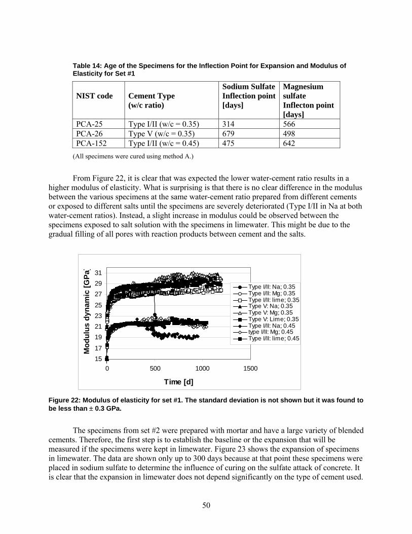
50

Table 14: Age of the Specimens for the Inflection Point for Expansion and Modulus of Elasticity for Set #1

NIST code

Cement Type (w/c ratio)

Sodium SulfateInflection point [days]

Magnesium sulfate Inflecton point [days]

PCA-25 Type I/II (w/c = 0.35) 314 566 PCA-26 Type V (w/c = 0.35) 679 498 PCA-152 Type I/II (w/c = 0.45) 475 642

(All specimens were cured using method A.)

From Figure 22, it is clear that was expected the lower water-cement ratio results in a

higher modulus of elasticity. What is surprising is that there is no clear difference in the modulus between the various specimens at the same water-cement ratio prepared from different cements or exposed to different salts until the specimens are severely deteriorated (Type I/II in Na at both water-cement ratios). Instead, a slight increase in modulus could be observed between the specimens exposed to salt solution with the specimens in limewater. This might be due to the gradual filling of all pores with reaction products between cement and the salts.

Figure 22: Modulus of elasticity for set #1. The standard deviation is not shown but it was found to be less than ± 0.3 GPa.

The specimens from set #2 were prepared with mortar and have a large variety of blended

cements. Therefore, the first step is to establish the baseline or the expansion that will be measured if the specimens were kept in limewater. Figure 23 shows the expansion of specimens in limewater. The data are shown only up to 300 days because at that point these specimens were placed in sodium sulfate to determine the influence of curing on the sulfate attack of concrete. It is clear that the expansion in limewater does not depend significantly on the type of cement used.

1517

19212325

272931

0 500 1000 1500

Time [d]

Mod

ulus

dyn

amic

[GPa

]

Type I/II: Na; 0.35Type I/II: Mg; 0.35Type I/II: lime; 0.35Type V: Na; 0.35Type V: Mg; 0.35Type V: Lime; 0.35Type I/II: Na; 0.45type I/II: Mg; 0.45Type I/II: lime; 0.45

51

Therefore, an average curve was calculated and shown as a solid line in Figure 23. This

calculated curve will be used as the baseline for the rest of the discussion on expansion results. The small expansion observed in these specimens in limewater is probably due to hydration of the cement paste and swelling due to water ingress. This expansion is never reported because it is not measured for 300 days and at 7 days is less than 0.005% (20 times smaller than the expansion determined as deleterious by ASTM C 1012).

Figure 23: Specimens in lime water for set #2

Figure 24 and Figure 25 show the expansion data for the blended cements used. Two curing periods were used. In method A, the specimens were placed after 24 hours from mixing in 100% RH in the testing solutions (sodium or magnesium sulfate). In method B, the specimens were kept in limewater for about 300 days before being placed in the testing solutions. Table 15 shows the exact duration of curing method B for all the cements used. The idea behind the two curing methods was to see the influence of curing duration on the expansion, modulus of elasticity, and microscopic structure.

From the expansion curves from either curing method, it could be determined that the addition of Class C fly ash (FA-C) leads to a higher rate of expansion than the control (Type I/II cement) at this dosage. At the other end of the spectrum, the specimen with silica fume (SF) did not expand at all compared to the specimens in limewater. The performance of the various cements could be ranked by their expansion at a certain date, but the best method is to determine the inflection point of the expansion curve versus time, which should be the longest for the cement most resistant to sulfate attack. Table 17 shows the inflection points. It should be noted that some specimens cured by method B have not yet deteriorated. The GGBFS-100 specimen was not measured with curing method B because there were no specimens available (broken during demolding). In the cases where the

limewater

0.0000.0050.010

0.0150.0200.0250.0300.035

0.0400.0450.050

0 50 100 150 200 250 300

Time [days]

Expa

nsio

n [%

]

controlFA-CFA-FShaleMKKaolin/opalGGBFS-80GGBFS-120SFaverage Lime

52

inflection point could be calculated (specimen deteriorated), it seems that the longer curing leads to a faster deterioration. The only exception is the control, where the inflection points are 3 days

Figure 24: Expansion of the specimens in set #2, curing method A. A) All data, B) close-up view of expansion below 0.25% for specimens of set #2 (A). The “Expansion in lime” shows the expansion for the specimens kept in limewater. The values of the expansion in lime later than 300 days are an extrapolation (see text). apart (25 days for curing method A and 28 days for curing method B). It could be argued that the time to the inflection point for the control specimen is relatively short and, therefore, the duration of curing does not have a major effect.

in Na2SO4

0.0

0.5

1.0

1.5

2.0

2.5

3.0

0 500 1000 1500 2000 2500

Time [d]

Expa

nsio

n [%

]

0.0

0.5

1.0

1.5

2.0

2.5

3.0

0 20 40 60 80

Time [months]

control

FA-C

FA-FMK

Kaolin/opal

GGBFS-80

GGBFS-100

GGBFS-120SF

Shale

Ain Na2SO4

0.00

0.05

0.10

0.15

0.20

0.25

0.30

0 100 200 300 400 500

Time [d]

Expa

nsio

n [%

]

0.0

0.1

0.1

0.2

0.2

0.3

0.30 5 10 15

Time [months]

control

FA-C

FA-F

MK

Kaolin/opal

GGBFS-80

GGBFS-100

GGBFS-120

SF

Shale

B

53

Figure 25: Expansion of set #2, after about 300 days curing in limewater (curing B). A) All data, B) close-up view of expansion below 0.25% for specimens of set #2 (A). The “Expansion in lime” shows the expansion for the specimens kept in limewater. The values of the expansion in lime later than 300 days are an extrapolation (see text).

Curing B

0.0

0.5

1.0

1.5

2.0

2.5

3.0

0 500 1000 1500 2000

Time [d]

Expa

nsio

n [%

]

0.0

0.5

1.0

1.5

2.0

2.5

3.0

0 20 40 60 80Time [months]

control

FA-C

FA-F

MK

Kaolin/opal

GGBFS-80

GGBFS-120

SF

Shale

ACuring B

0.00

0.05

0.10

0.15

0.20

0.25

0.30

0 100 200 300 400 500

Time [d]

Expa

nsio

n [%

]

0.0

0.1

0.1

0.2

0.2

0.3

0.3

0 5 10 15Time [months]

control

FA-C

FA-F

MK

Kaolin/opal

GGBFS-80

GGBFS-120

SF

Shale

B

54

Table 15: Duration of Curing for Method B

NIST code SCM Name

Curing Duration of Curing B [days]

PCA-174 None A,B 346 PCA-175 Fly Ash F A,B 343 PCA-180 Fly Ash C A,B 342 PCA-191 Metakaolin A,B 342 PCA2-12 Calcined Montmorillonite

(Shale) A,B 312

PCA2-13 Calcined Kaolin/Opal A,B 311 PCA2-24 GGBFS 80 A,B 305 PCA-193 GGBFS 100 A,B* 340 PCA2-23 GGBFS 120 A,B 306 PCA2-28 Silica Fume A,B 304

Note: *Only prisms for measuring the modulus were available for curing B.

Table 16: Age of the Specimens for the Inflection Point for Expansion and Modulus of Elasticity for Set #2

NIST code SCM Name

Curing A Inflection point [days]

Curing B Inflection point [days]

PCA-174 None 25 28 PCA-175 Fly Ash F 339 >300 PCA-180 Fly Ash C 80 28 PCA-191 Metakaolin 403 >300 PCA2-12 Calcined Montmorillonite

(Shale) >600 >300

PCA2-13 Calcined Kaolin/Opal 330 >300 PCA2-24 GGBFS 80 382 168 PCA-193 GGBFS 100 500 >300 PCA2-23 GGBFS 120 218 112 PCA2-28 Silica Fume >600 >300

Note: “>600” or “>300” indicates that the specimens have not yet reached the inflection point and the measurements were recorded for about 600 or 300 days, as of this writing.

Figure 26 and Figure 27 show the data obtained from the measurements for the modulus of elasticity. Although not as clear as for the expansion measurements, the same deterioration could be determined. The deterioration of the specimen is determined by a decrease in the modulus of elasticity, which is a sign that cracks may have appeared and the microstructure was changed or weakened. The following observations can be made:

• The control and FA-C show a decrease in the modulus at an earlier age than any other specimens.

55

• SF specimens' modulus of elasticity is comparable to the specimens kept in limewater and even show a slight increase over time.

• The other specimens are deteriorating at the same rate as seen in the expansion curves.

Figure 26: Modulus of elasticity for set #2 in sodium sulfate curing method A. The standard deviation is not shown but it was found to be less than ± 0.3 GPa.

Figure 27: Modulus of elasticity of the specimens of set #2 after curing method B (almost 300 days). The standard deviation is not shown but it was found to be less than ± 0.3 GPa.

Curing A

0

5

10

15

20

25

30

35

40

45

0 200 400 600 800 1000

Time [d]

Mod

ulus

dyn

amic

[GPa

] controlFA-CFA-FShaleMKKaolin/opalGGBFS-80GGBFS-100GGBFS-120SFaverage Lime

Curing B

15

20

25

30

35

40

45

0 100 200 300 400

Time [d]

Mod

ulus

Dyn

amic

[GPa

]

controlFA-CFA-FShaleMKKaolin/opalGGBFS-80GGBFS-100GGBFS-120SFaverage Lime

56

Table 17: Age of the Specimens for the Inflection Point for Expansion and Modulus of Elasticity for Set #2

NIST code SCM Name

Curing A Inflection point [days]

Curing B Inflection point [days]

PCA-174 None 25 28 PCA-175 Fly Ash F 339 1100 PCA-180 Fly Ash C 80 28 PCA-191 Metakaolin 403 1100 PCA2-12 Calcined Montmorillonite

(Shale) >1800 >1500

PCA2-13 Calcined Kaolin/Opal 330 1100 PCA2-24 GGBFS 80 382 168 PCA-193 GGBFS 100 500 NA PCA2-23 GGBFS 120 218 112 PCA2-28 Silica Fume >1800 >1500

Note: “>T” indicates that the specimens have not yet reached the inflection point and the measurements were recorded for about T days, as of this writing.

The data from the standard tests (ASTM C 1012) prepared by California Portland Cement

Company (CPC) are shown in Figure 28. The same trend is noticed: a) FA-C specimens expand faster and more than the control and b) Type I cement is more expansive than cement Type V. After a full year of measurements, it is hard to distinguish between the rest of the cements. They all expanded less than the 0.1% required for a sulfate resistant cement. These observations for the blended cements (with the exception of the FA-C) are identical to the data obtained at NIST after one year. These results could lead to the conclusion that all the blended cements with the exception of FA-C are sulfate resistant, but the conclusion might be premature as when the measurements are continued, as was done at NIST for over five years4. From Figure 24 and Figure 25, it is clear that only the SF and shale addition in cement are still not expanding after five years. All the other blended cements are destroyed after about 2.5 years. This is a demonstration that several factors are affecting expansion and they need to be better understood to be able to properly predict cement performance. Just measuring expansion according to ASTM C 1012 for a year will not provide a clear picture of the performance of supplementary cementitious materials.

It should also be noted that the expansion measured at NIST is larger for all specimens than the expansions measured by the independent laboratory. It is unclear why the measurements differ, but the same conclusions can be drawn from the trends and the relative comparison of the various cements.

4 It should be kept in mind that the standard ASTM C 1012 tests are usually conducted only for one year while NIST measurements were conducted to failure, e.g., in some case as long as five years.

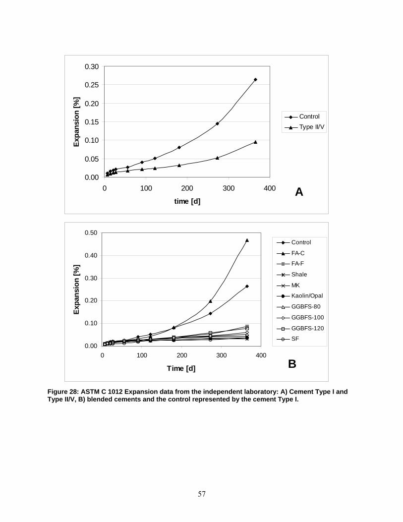
57

Figure 28: ASTM C 1012 Expansion data from the independent laboratory: A) Cement Type I and Type II/V, B) blended cements and the control represented by the cement Type I.

0.00

0.05

0.10

0.15

0.20

0.25

0.30

0 100 200 300 400

time [d]

Expa

nsio

n [%

]

ControlType II/V

A

0.00

0.10

0.20

0.30

0.40

0.50

0 100 200 300 400

Time [d]

Expa

nsio

n [%

]

Control

FA-C

FA-F

Shale

MK

Kaolin/Opal

GGBFS-80

GGBFS-100

GGBFS-120

SF

B

58

Microstructure Observations To better understand the effects of sulfate exposure on hardened cement paste microstructure, a petrographic study is necessary. The SEM provides image contrast and X-ray microanalysis to facilitate identification of the constituent phases within a microstructure. Sampling the specimens as exposure tests proceed should enable us to construct a picture of the changes in the hardened cement paste with depth, over time. These data may allow a more complete description of the failure mechanisms and suggest means to devise an accelerated testing procedure. X-ray powder diffraction provides qualitative and quantitative mineralogical information, complimentary to the microscopy. In this study, the XRD data were used to identify the crystalline hydration products in portions of the affected cement paste. The Scanning Electron Microscope (SEM). The SEM scans a focused beam of electrons across the specimen and measures any of several signals resulting from the electron beam interaction with the specimen. Images of topography can be used to study particle size, shape, surface roughness, and fracture surfaces, while polished surfaces are used for determination of phase distribution and chemical composition. X-ray microanalysis provides qualitative and semiquantitative spot chemical analysis as well as maps of element distribution of hydration products. The combination of backscattered electron (BE) and X-ray (XR) imaging is the most useful imaging mode for quantitative determination of phase distribution and chemical composition. Backscattered electrons are high-energy electrons scattered by the specimen. BE image contrast is generated by the different phases' compositions (their average atomic number) and is observed as the differential brightness in an image. Anhydrous cement appears brightest, followed by calcium hydroxide, gypsum, calcium silicate hydrate, ettringite and monosulfate, and aggregate; voids appear dark (Figure 29).

X-rays are produced when a specimen is bombarded by high-energy electrons. With an energy-dispersive detector, the X-ray energy level is displayed as the number of counts at each energy interval and appears as a set of peaks on a continuous background. The positions of the peaks are characteristic of a particular element, so identifications are made by examination of peak positions and relative intensities. The X-ray signal can be used for: a) spectrum analysis to determine which elements are present and in what concentration, b) line scan analysis to display the relative concentration changes along a line, and c) X-ray imaging (XR) of element spatial distribution and relative concentrations, to aid in phase identification. Mass concentration to a few tenths of a percent can be detected using an energy-dispersive X-ray detector with relative accuracy of quantitative analysis (using certified standards), about ± 20% for concentrations around 1% and ± 2% for concentrations greater than 50% for ideal specimens. However, paste heterogeneity and the likelihood of decomposition under a high-energy electron beam makes these analyses only semiquantitative. Previous studies used plots of atom ratios and consider the relative differences of greater importance than the absolute values. More details on X-ray microanalysis may be found in Goldstein et al. [64].

Feature resolution is dependent upon instrument operating conditions, imaging mode, and phase density. Secondary electron imaging resolution may approach nanometer-size, while image resolution for the BE is approximately 0.25 μm and, for the X-ray images, about 1 μm.

59

Specimens are prepared using an epoxy-replacement method developed at NIST [65] where the pore solution is replaced by alcohol, and then the alcohol is replaced by epoxy without drying or any associated drying shrinkage. Specimens are prepared with a low-viscosity epoxy5 which is then cured at low temperature (60°C to 65°C) for 24 hours.

A fresh surface is exposed through grinding and then is polished using a series of successively finer grades of diamond paste. This polishing stage removes the cutting and grinding damage, exposing a cross section of the material's microstructure. Epoxy impregnation of the pore system serves two purposes: a) it fills voids and, upon curing, supports the microstructure, restraining it against shrinkage cracking, and b) it enhances contrast between the pores, hydration products, and cementitious material. Cracks observed using this preparation might then be ascribed to physical or chemical processes acting upon the concrete, and not due to drying-related shrinkage [65].

A thin coating of carbon serves to dissipate excess charge from the specimen while exhibiting little effect on image contrast and no interference with elements of interest. Semiquantitative elemental analyses are standardized using well-characterized reference glass and mineral specimens from NIST and the Museum of Natural History of the Smithsonian Institution [66].

X-ray powder diffraction analysis of crushed, sieved (100 μm passing) powders is also used to assess the crystalline products of the outer 3 mm and cores from each specimen.

Figure 29: 0.45 w/c, 7-day-old hardened cement paste (field width, 25 μm).

5 L.R. White, hard grade. London Resin Company.

Calcium Hydroxide

Calcium –Silicate-Hydrate Monosulfate

Residual Cement

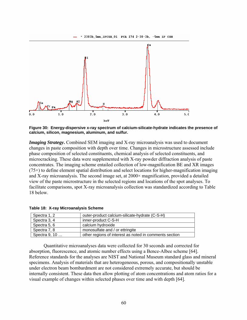
60

Figure 30: Energy-dispersive x-ray spectrum of calcium-silicate-hydrate indicates the presence of calcium, silicon, magnesium, aluminum, and sulfur.

Imaging Strategy. Combined SEM imaging and X-ray microanalysis was used to document changes in paste composition with depth over time. Changes in microstructure assessed include phase composition of selected constituents, chemical analysis of selected constituents, and microcracking. These data were supplemented with X-ray powder diffraction analysis of paste concentrates. The imaging scheme entailed collection of low-magnification BE and XR images (75×) to define element spatial distribution and select locations for higher-magnification imaging and X-ray microanalysis. The second image set, at 2000× magnification, provided a detailed view of the paste microstructure in the selected regions and locations of the spot analyses. To facilitate comparisons, spot X-ray microanalysis collection was standardized according to Table 18 below.

Table 18: X-ray Microanalysis Scheme

Spectra 1, 2 outer-product calcium-silicate-hydrate (C-S-H) Spectra 3, 4 inner-product C-S-H Spectra 5, 6 calcium hydroxide Spectra 7, 8 monosulfate and / or ettringite Spectra 9, 10 … other regions of interest as noted in comments section

Quantitative microanalyses data were collected for 30 seconds and corrected for

absorption, fluorescence, and atomic number effects using a Bence-Albee scheme [64]. Reference standards for the analyses are NIST and National Museum standard glass and mineral specimens. Analysis of materials that are heterogeneous, porous, and compositionally unstable under electron beam bombardment are not considered extremely accurate, but should be internally consistent. These data then allow plotting of atom concentrations and atom ratios for a visual example of changes within selected phases over time and with depth [64].

61

X-ray Powder Diffraction Analysis (XRD). X-ray powder diffraction (XRD) allows identification of crystalline products in the cement paste. To facilitate identification, the cement paste fraction was removed from each specimen by gentle crushing by mortar and pestle and then sieving through a 125 μm sieve. To reduce any effects of carbonation, each powder was separated just prior to analysis. These data provide another means of assessing the types and relative abundance of phases such as ettringite, gypsum, monosulfate, and calcium hydroxide over time and with depth. Each specimen was sampled to provide two powder specimens: one from the outer 2 to 3 mm and one from the core paste.

Alteration effects are seen after a few days’ exposure of cement paste to sulfate solutions (50 g/L Na2SO4, the same concentration as in ASTM C 1012) with the replacement of CH by gypsum in the outer portions of the cement paste. However, this replacement does not appear to be disruptive. This replacement forms a front that migrates inward with time and progresses to a depth of a few millimeters. Eventually, three zones outside of the apparently unaltered cement paste become distinct: 1) An outer zone leached of most constituents (including ettringite), leaving a more porous, calcium-depleted C-S-H and some remnant ferrite, 2) a second zone where gypsum replaces calcium hydroxide and ettringite replaces monosulfate, and 3) a third zone with monosulfate that appears to be sulfur-rich or perhaps a mixture of ettringite and monosulfate. At later stages of testing, specimens exhibit cracking parallel to the exterior in the outer zones, with the fractures generally filled by gypsum.

Figure 31 shows a wide-area view (about 4 mm) of the mortar bar with an outer surface to the left. Cracking parallel to the surface is highlighted by the gypsum-filled cracks demonstrated by the high sulfur regions of the X-ray image (upper left) and the lighter phase rimming the sand grains in the lower-right higher-magnification image. The presence of gaps along aggregate boundaries is an indication that the hardened cement paste matrix has expanded. The slight decrease in overall intensity in the calcium image and backscattered electron (BSE) image reflects the calcium depleted outer zone. The gypsum is generally confined to this outer portion of the mortar, and microanalysis evidence indicates changes in monosulfate and calcium aluminate phases at greater depths that probably are contributing to the expansion.

Figure 32 provides a higher-magnification, cross-sectional view of a hardened cement paste in a limewater-cured, control mortar specimen. The outer surface is oriented to the left, with a total field width of 250 μm. The residual cement grains appear brightest followed by calcium hydroxide (CH), calcium-silicate-hydrate (C-S-H), and dark voids that are filled with epoxy. The C-S-H may be further subdivided into outer-C-S-H, formed in the originally water-filled spaces, and inner-C-S-H, formed by in-situ hydration of the cement grains. The outer-C-S-H has a coarser porosity and so appears slightly darker. Other constituents such as ettringite (AFt) and monosulfate (AFm) occur in the bulk paste and may be identified based upon their textures and chemical signatures.

Figure 33 shows a cross section of hardened cement paste (250 μm field width) that has been exposed to the sodium sulfate solution for 105 days, exhibiting 0.14% expansion. Changes in microstructure relative to the control include an increased porosity near the surface, and a loss of CH within 150 μm of the surface. A second zone may be characterized by replacement of monosulfate with ettringite, a densification of inner-product C-S-H (seen as a loss of coarse-capillary porosity), and deposition of gypsum in place of CH. At greater depths, the spot chemical analysis indicates increased sulfate content in the C-S-H relative to the control and mixtures of monosulfate and ettringite in regions formerly occupied by monosulfate. The first

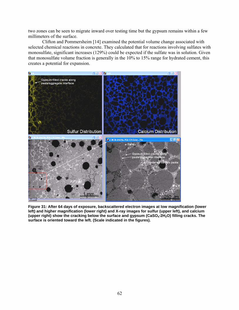
62

two zones can be seen to migrate inward over testing time but the gypsum remains within a few millimeters of the surface.

Clifton and Pommersheim [14] examined the potential volume change associated with selected chemical reactions in concrete. They calculated that for reactions involving sulfates with monosulfate, significant increases (129%) could be expected if the sulfate was in solution. Given that monosulfate volume fraction is generally in the 10% to 15% range for hydrated cement, this creates a potential for expansion.

Figure 31: After 64 days of exposure, backscattered electron images at low magnification (lower left) and higher magnification (lower right) and X-ray images for sulfur (upper left), and calcium (upper right) show the cracking below the surface and gypsum (CaSO4·2H2O) filling cracks. The surface is oriented toward the left. (Scale indicated in the figures).

63

Figure 32: Cross section of hardened cement paste not exposed to sulfate solution, showing residual cement grains, calcium hydroxide (CH), calcium-silicate-hydrate (CSH), monosulfate (AFm), and voids.

Figure 33: Type I/II cement paste (105 days of exposure to sulfate solution), Na2SO4-soaked specimen, showing increased porosity near the surface (left, zone 1), loss of calcium hydroxide in outer 150 μm (zones 1 & 2), possible densification of inner-product CSH in CH-depleted zone 2, deposition of gypsum in place of CH, and replacement of monosulfate with ettringite.

Small Prisms New Test Specimens that fail the ASTM C 1012 test often exhibit no-length change for a certain period after exposure to sulfate followed by a rapid increase in length as shown above. Imaging a specimen after this increase shows a number of interesting phenomena that may explain its cause. A composite image (Figure 34, about 12 mm total field width) of the BSE image of the mortar (bottom) and X-ray images of sulfur (top) with the mortar bar end oriented to the left shows the measuring pin as the brightest object in the BSE image. Two features are evident: 1) the gypsum-rich regions extend deeper into the bar at the ends relative to the central part of the bar and 2) the expansive reactions in the end have lifted the measurement pin about 0.50 mm out of its socket.

64

The sulfate solution has penetrated from both the end and side surfaces of the bar. This penetration from multiple directions results in the bar ends being more completely affected than the midlength portions of the bar. The highly affected area (as defined by gypsum-filled cracking parallel to the surfaces) extends about half the length of the pin, which is then lifted by the expansion of the outer mortar. This would indicate that the early expansion measured is not the result of the entire cross section reacting to the sulfate infiltration and that the core, up to that point, has served to restrain expansion. The measurement of expansion according to ASTM C 1012 is based on the assumption that the whole specimen is expanding at the same time, while what we observed is that only a small fraction around the pin is responsible for the bulk of the measured expansion. Therefore, given this specimen configuration and lack of protection of the end portions, only a fraction of the whole standard specimen is really affected by the sulfate. As expansion is measured as a percentage of the total length affected, the real expansion near the pin could be 50 times larger than reported. By real expansion, we mean the change in length due to the chemical reaction divided by the length of affected specimen.

Therefore, two solutions to the deterioration around the pin and in the outer layer are proposed: 1) protect the ends of the specimens so that the sulfate penetration cannot occur from these surfaces and around the pin and 2) reduce the cross section of the specimens to shorten the time necessary to permeate the specimen with the sulfate. The combination of these modifications will protect the end surfaces and pin region from sulfate penetration while decreasing the time for the solution to permeate the test bar cross section. This should produce a more effective configuration to measure expansion of the whole specimen (not just the outer layer or around the pins).

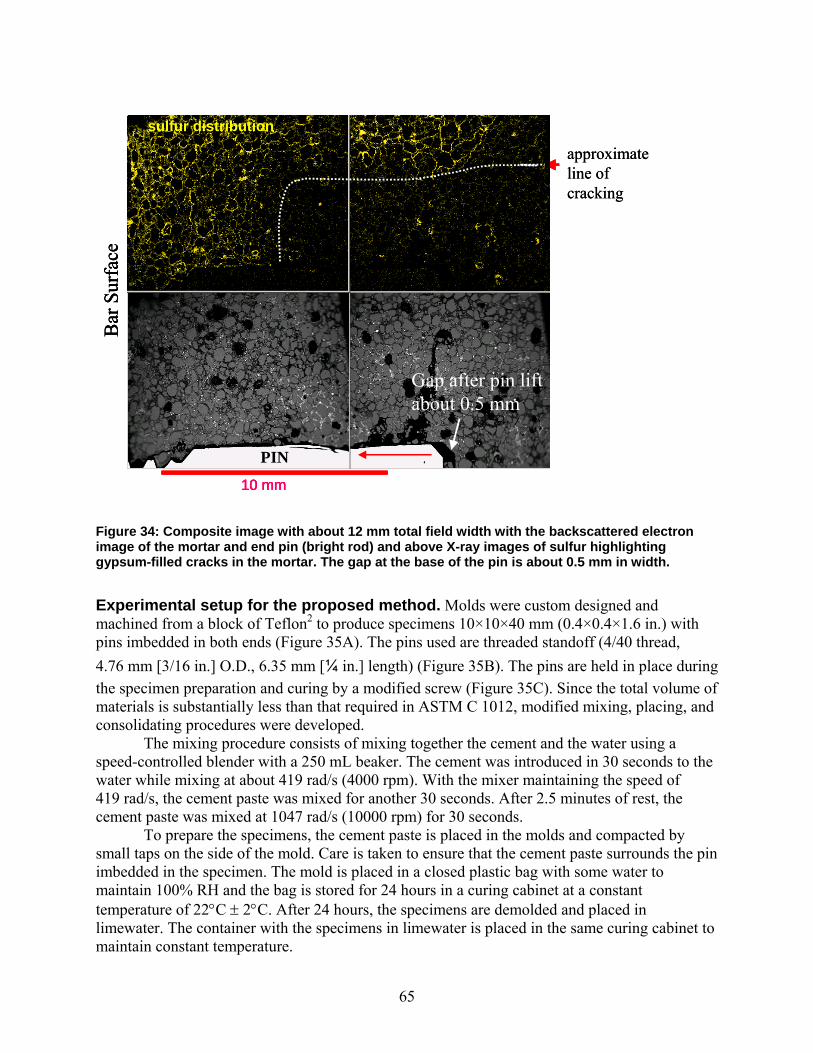
65

Figure 34: Composite image with about 12 mm total field width with the backscattered electron image of the mortar and end pin (bright rod) and above X-ray images of sulfur highlighting gypsum-filled cracks in the mortar. The gap at the base of the pin is about 0.5 mm in width.

Experimental setup for the proposed method. Molds were custom designed and machined from a block of Teflon2 to produce specimens 10×10×40 mm (0.4×0.4×1.6 in.) with pins imbedded in both ends (Figure 35A). The pins used are threaded standoff (4/40 thread, 4.76 mm [3/16 in.] O.D., 6.35 mm [¼ in.] length) (Figure 35B). The pins are held in place during the specimen preparation and curing by a modified screw (Figure 35C). Since the total volume of materials is substantially less than that required in ASTM C 1012, modified mixing, placing, and consolidating procedures were developed.

The mixing procedure consists of mixing together the cement and the water using a speed-controlled blender with a 250 mL beaker. The cement was introduced in 30 seconds to the water while mixing at about 419 rad/s (4000 rpm). With the mixer maintaining the speed of 419 rad/s, the cement paste was mixed for another 30 seconds. After 2.5 minutes of rest, the cement paste was mixed at 1047 rad/s (10000 rpm) for 30 seconds.

To prepare the specimens, the cement paste is placed in the molds and compacted by small taps on the side of the mold. Care is taken to ensure that the cement paste surrounds the pin imbedded in the specimen. The mold is placed in a closed plastic bag with some water to maintain 100% RH and the bag is stored for 24 hours in a curing cabinet at a constant temperature of 22°C ± 2°C. After 24 hours, the specimens are demolded and placed in limewater. The container with the specimens in limewater is placed in the same curing cabinet to maintain constant temperature.

approximateline of cracking

Bar

Sur

face

Sulfur Distribution

PIN

Gap after pin liftabout 0.5 mm

sulfur distribution

10 mm

approximateline of cracking

Bar

Sur

face

Sulfur Distribution

PIN

Gap after pin liftabout 0.5 mm

sulfur distribution

10 mm

Bar

Sur

face

Sulfur Distribution

PIN

Gap after pin liftabout 0.5 mm

sulfur distribution

10 mm10 mm

66

Three or four days after mixing, the specimens are removed from the limewater and a threaded stud is screwed in the end pins (Figure 36 and Figure 37A). The threaded stud is 12.7 mm long and has the same thread as the pin (4/40). To ensure that the stud does not move during the expansion experiment a small amount of epoxy is placed around one end of the studs and threaded into the specimen ends. Epoxy is applied to both end faces around the studs and 5 mm on the top side of the specimen to prevent sulfate penetration from the ends (Figure 36). The epoxy is cured by leaving the specimens in a 100% RH environment for about 5 to 6 hours. Water should not contact the specimen or the epoxy during this curing. The specimens are then returned to the limewater until the start of exposure to sulfate solution, usually 7 days after casting. During exposure to the sulfate solution, specimens are kept in a temperature controlled cabinet at 23°C ± 0.5°C.

A length change comparator (Figure 37B) is used to measure expansion with a stainless steel or, if possible, Invar cylinder (Figure 37A) as a reference length to zero the comparator. The pins for the comparator are custom fabricated to accommodate the studs of the specimens.

After curing, the specimens are measured and placed in a sulfate solution 50 g/L Na2SO4 (the same solution as in ASTM C 1012). It is strongly suggested that the container with the specimens be kept at constant temperature to reduce length changes from temperature fluctuations. This is not done in the ASTM standard test as the volume of the specimen and container are less susceptible to small fluctuations in temperature. The controlled temperature reduces the scatter significantly, especially during the first few days [67]. The specimens are then measured every day for the first two weeks and then once a week until deterioration commences.

67

Figure 35: Molds for specimens: A) general view, B) pin imbedded in the specimen, and C) screw to hold pins in place during cast.

A

CB

Pins imbedded in specimen

Screws holding pin in place

A

CB

Pins imbedded in specimen

Screws holding pin in place

68

Figure 36: Specimens with epoxy coated ends. Specimen D was also coated 5 mm on the side; Specimen A had only the end sections coated. It was determined that the D-type coating gave more reproducible results [67].

Figure 37: Expansion measurement: A) reference and a specimen, B) comparator with the reference in place.

69

Results and discussion. The goals of the test program for measuring expansion were to: 1) check that the expansion could be measured using small specimens, 2) determine the reproducibility of the measurements, and 3) compare the results with those obtained with the larger (ASTM C 1012) specimens. In all cases, the cement performance was compared with cement with the addition of SCM.

Two sets of small specimens were prepared: 1) mortars and 2) neat cement paste. Distinct differences emerged upon comparing mortar and paste-only specimens (Figure 38) with mortar specimens showing greater expansion than the corresponding cement pastes. This could be explained by the faster penetration of the sulfate through the more permeable mortar. However, the mortar specimens do not show a difference in expansion between the two cements (FA-C and control), while there is a significant difference after 20 days for the cement paste specimens. After 40 days of measurement, the mortar and the cement paste specimens were “no longer measurable.” The definition of “no longer measurable” indicates that either the specimen is too long for the comparator, or the specimen is in a very poor state or disintegrated.

Repeatability in mortars is poorer than that for the cement paste as seen in the larger error bar widths. Intrinsically, mortar specimens have a more random microstructure due to the random aggregate structure superimposed on the cement paste microstructure. Also, the difficulty in casting and consolidating small mortar specimens, especially in consolidation around the pin area, lessens the repeatability. No problems with casting and consolidation were observed using neat cement paste, and elimination of the sand reduces preparation efforts. Therefore, the cement paste specimens appear to provide faster and more reliable results than the mortar specimens.

The results presented in Figure 38 are from five specimens for each composition. The selection of the five replicates is somewhat arbitrary and further studies could be conducted to determine if the number can be reduced. The risk of selecting fewer specimens is potentially higher scatter in the results. Larger prisms according to ASTM C 1012 and comparison with small prisms Figure 39 shows results obtained using the standard prism specimens in ASTM C 1012 (25.4×25.4×285 mm). The ranking of the resistance to sulfate attack is the same as for the smaller cement paste specimens, e.g., the specimens with Class C fly ash expand more than the controls during the time of the measurements.

As is done in ASTM C 1012 [68, 69], the time to reach an expansion of 0.1% was taken as the critical time to classify the performance of the cements. Table 19 shows the results. The small cement paste specimens ranked the cements in about 20 to 30 days, while the large specimen required twice the time while ranking the control as worse or identical to the cement with fly ash. If the testing stopped at this point, the conclusions reached with the large prisms would not be a valid assessment of the resistance of these cements, as it is known that addition of FA-C is deleterious for sulfate resistance of cement paste. In Table 19 we also show the expansion reached at an arbitrary later date, 30 days for small specimens and 100 days for the larger specimens. We could not select the same date for both types of specimens because 1) the large specimens at 30 days were below 0.1% expansion, 2) the small specimens were not longer measurable after 30 days, and 3) at 120 days the FA-C large specimens were no longer measurable. Therefore, from Figure 37B and Figure 38 and from Table 19, it could be inferred that the FA-C cement is less sulfate resistant than the control. The results for small specimens

70

mirror those for larger specimens and provide a result in a third to a fifth of the time for the cements shown here that were highly reactive.

Obviously, these preliminary observations of the relative behavior of the two types of specimens should be verified with further testing of various cements.

Figure 38: Average expansion of small specimens versus time: A) mortar specimens and B) cement paste specimens. The standard deviations of the five specimens are shown as error bars.

Figure 39: Average expansion of large specimens versus time. The standard deviations of the three specimens are shown as error bars. For FA-C, the error bars are smaller than the data symbol.

-0.10

0.00

0.10

0.20

0.30

0.40

0.50

0.60

0 10 20 30 40

Time [d]

Expa

nsio

n [%

]

Neat

FA-C

A0.00

0.05

0.10

0.15

0.20

0.25

0.30

0.35

0 10 20 30 40

Time [d]

Expa

nsio

n [%

]

Neat

FA-C

B

0.00

0.10

0.20

0.30

0.40

0.50

0.60

0 20 40 60 80 100 120

Time [d]

Expa

nsio

n [%

]

control

FA-C

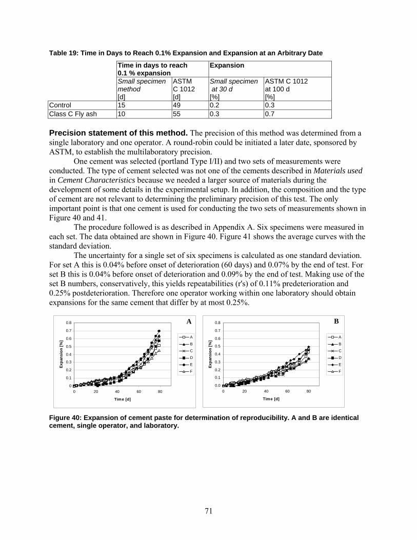
71

Table 19: Time in Days to Reach 0.1% Expansion and Expansion at an Arbitrary Date

Time in days to reach 0.1 % expansion

Expansion

Small specimen method [d]

ASTM C 1012 [d]

Small specimen at 30 d [%]

ASTM C 1012 at 100 d [%]

Control 15 49 0.2 0.3 Class C Fly ash 10 55 0.3 0.7 Precision statement of this method. The precision of this method was determined from a single laboratory and one operator. A round-robin could be initiated a later date, sponsored by ASTM, to establish the multilaboratory precision.

One cement was selected (portland Type I/II) and two sets of measurements were conducted. The type of cement selected was not one of the cements described in Materials used in Cement Characteristics because we needed a larger source of materials during the development of some details in the experimental setup. In addition, the composition and the type of cement are not relevant to determining the preliminary precision of this test. The only important point is that one cement is used for conducting the two sets of measurements shown in Figure 40 and 41.

The procedure followed is as described in Appendix A. Six specimens were measured in each set. The data obtained are shown in Figure 40. Figure 41 shows the average curves with the standard deviation.

The uncertainty for a single set of six specimens is calculated as one standard deviation. For set A this is 0.04% before onset of deterioration (60 days) and 0.07% by the end of test. For set B this is 0.04% before onset of deterioration and 0.09% by the end of test. Making use of the set B numbers, conservatively, this yields repeatabilities (r's) of 0.11% predeterioration and 0.25% postdeterioration. Therefore one operator working within one laboratory should obtain expansions for the same cement that differ by at most 0.25%.

Figure 40: Expansion of cement paste for determination of reproducibility. A and B are identical cement, single operator, and laboratory.

0

0.1

0.2

0.3

0.4

0.5

0.6

0.7

0.8

0 20 40 60 80

Time [d]

Expa

nsio

n [%

]

A

B

C

D

E

F

A

0.0

0.1

0.2

0.3

0.4

0.5

0.6

0.7

0.8

0 20 40 60 80

Time [d]

Expa

nsio

n [%

]

A

B

C

D

E

F

B

72

Figure 41: Average curve of data shown in Figure 40. Conclusion This section presented a new and more rapid method based on materials science to measure expansion of cement paste exposed to a sulfate solution. This method is based on petrographic examination of specimens exposed to sulfate and uses smaller test specimens than those utilized in the current standard tests (ASTM C 1012). The same conclusions on the potential sulfate resistance of a cement can be obtained using either method, but the new method described here requires less than one third the testing time compared to ASTM C 1012.

This study exposed some problems inherent with the current test method described in ASTM C 1012. Permeation of the test solution occurs along the mortar bar ends, sides, and pins resulting in the measurement of reaction and expansion of only a portion of the test specimen. If this issue was corrected, the standard specimens will likely take even longer to expand to the deleterious level. By using a paste test specimen with a smaller cross section and protected ends we were able to reduce testing time and measure the expansion due to sulfate interaction with cement paste hydration products across the entire test specimen. Temperature control becomes paramount when small specimens are used and helps reduce the scatter of the data, especially at early testing ages.

This study presented only some of the data available and it needs to be further validated by conducting tests on a larger selection of cements, SCMs, and varying replacement levels.

0.0

0.1

0.2

0.3

0.4

0.5

0.6

0.7

0.8

0 20 40 60 80 100

Time [d]

Expa

nsio

n [%

]

Series A

Series B

Average

A

73

CONCLUSIONS The scope of this project was to develop a methodology to determine the resistance to sulfate attack of a cement and/or a concrete. The goal was to develop faster methods than those presently used, which as described in ASTM take between six months and one year. The method developed was based on ASTM E 632. The determination of the resistance of cement paste and concrete was separated by the properties affecting the deterioration from the sulfate attack. Therefore, the products from this study were:

For the concrete: • Sorption test • Methodology to estimate diffusion of sulfate into concrete • A methodology to evaluate the resistance of concrete to sulfate attack under wet-dry

cycles For the cement paste: • A methodology to determine the deterioration of the cement from small specimens • Some models to predict the deterioration of cement paste and concrete under sulfate

attack

More work still needs to be done before this methodology becomes fully accepted, but at least one test, sorption test, has been accepted by ASTM [52]. The small specimens test and the wetting-drying cycle method could be submitted to ASTM in the future. ACKNOWLEDGEMENTS The research reported in this paper (PCA R&D Serial No. 2486) was conducted by NIST, with the sponsorship of the Portland Cement Association (PCA Project Index No. 99-07). The contents of this paper reflect the views of the authors, who are responsible for the facts and accuracy of the data presented. The contents do not necessarily reflect the views of the Portland Cement Association.

The authors would like to thank the Portland Cement Association and NIST for their financial support. Also, John Winpigler performed all the tests on the standard prisms and Max Peltz was instrumental in finalizing the small specimens tests procedure. Stefan Leigh performed the statistical analysis for the precision statement for the small specimens test method proposed. Paul Tennis (PCA Consultant), Edward Garboczi (NIST), and Jeff Bullard (NIST) are recognized for their fruitful comments on this paper.

74

REFERENCES

1. “Standard Test Method for Length Change of Hydraulic-Cement Mortars Exposed to a Sulfate Solution,” ASTM C 1012-04, Annual Book of ASTM Standards, Volume 04.01, ASTM International, West Conshohocken, Pennsylvania, USA.

2. Skalny, J.; Marchand, J., and Odler, I., Sulfate Attack on Concrete, Spon Press, London, 2002.

3. Clifton, J.; Frohnsdorff, G., and Ferraris, C., “Standards for Evaluating the Susceptibility of Cement-Based Materials to External Sulfate Attack,” Materials Science of Concrete: Sulfate Attack Mechanisms –Special Volume; Ed. J. Marchand and J. P. Skalny, 1999.

4. Moir, G., Development of Sulfate Resistance Performance Test for Cements, Report by CEN TC51/WG12/TG1, 1999.

5. “Standard Practice for Developing Accelerated Tests to Aid Prediction of the Service Life of Building Components and Materials,” ASTM E 632-82(1996) (Withdrawn 2005), Annual Book of ASTM Standards, Volume 14.04. ASTM International, West Conshohocken, Pennsylvania, USA.

6. Brown, P.W., “An Evaluation of the Sulfate Resistance of Cements in a Controlled Environment,” Cement and Concrete Research, Vol. 11, pages 719 to 727, 1981.

7. Marchand, J., “Modeling the Behavior of Unsaturated Cement Systems Exposed to Aggressive Chemical Environment,” Materials and Structures, Vol. 34, pages 195 to 200, May 2001.

8. Tyrrell, H.J.V., and Harris, K.R., Diffusion in Liquids, Butterworths, London, 1984.

9. Crank, J., The Mathematics of Diffusion, 2nd Edition, Oxford University Press, London, 1975.

10. Helfferich, F., Ion Exchange, McGraw-Hill, New York, 1962.

11. Rubinstein, I., Electro-Diffusion of Ions, Society for Industrial and Applied Mathematics, Philadelphia, Pennsylvania, USA, 1990.

12. Samson, E., and Marchand, J., “Numerical Solution of the Extended Nernst-Planck Model,” J. Colloid Interface Sci., Vol. 215, pages 1 to 8, 1999.

13. Samson, E.; Marchand, J.; Robert, J.-L., and Bournazel, J.-P., “Modeling Ion Diffusion Mechanisms in Porous Media,” Int. J. Numer. Meth. Eng., Vol. 46, pages 2043 to 2060, 1999.

14. Tang, L., “Concentration Dependence of Diffusion and Migration of Chloride Ions, Part 1: Theoretical Considerations,” Cement Concrete Research, Vol. 29, pages 1463 to 1468, 1999.

15. Tang, L., “Concentration Dependence of Diffusion and Migration of Chloride Ions, Part 2: Experimental Evaluations,” Cement Concrete Research, Vol. 29, pages 1469 to 1474, 1999.

75

16. Truc, O.; Ollivier, J.-P., and Nilsson, L.-O., “Numerical Solution of Multi-Species Diffusion,” Materials and Structures, Vol. 33, pages 566 to 573, 2000.

17. Truc, O.; Ollivier, J.-P., and Nilsson, L.-O., “Numerical Simulation of Multi-Species Transport Through Saturated Concrete During a Migration Test - msdiff Code,” Cement Concrete Research, Vol. 30, pages 1581 to 1592, 2000.

18. Snyder, K.A., “The Relationship between the Formation Factor and the Diffusion Coefficient of Porous Materials Saturated with Concentrated Electrolytes: Theoretical and Experimental Considerations,” Concrete Science and Engineering, Vol. 3, pages 216 to 224, 2001.

19. Snyder, K.A., and Marchand, J., “Effect of Speciation on the Apparent Diffusion Coefficient in Nonreactive Porous Systems,” Cement and Concrete Research, Vol. 31, pages 1837 to 1845, 2001.

20. Collins, R.E., Flow of Fluids Through Porous Materials, Reinhold Publishing, New York, 1961.

21. Kato, M., “Numerical analysis of the Nernst-Planck-Poisson system,” J. Theor. Biol., Vol. 177, pages 299 to 304, 1995.

22. James, A.E.; Stillman, J. D., and Williams, D.J.A., “Finite Element Solution of the Equations Governing the Flow of Electrolyte in Charged Microporous Membranes,” Int. J. Numer. Meth. Fluid, Vol. 20, pages 1163 to 1178, 1995.

23. Gordon, A.R., “The Diffusion Constant of an Electrolyte, and its Relation to Concentration,” J. Chem. Phys., Vol. 5, pages 522 to 526, 1937.

24. Price, W.E.; Mills, R., and Woolf, L.A., “Use of Experimental Diffusion Coefficients to Probe Solute-Solute and Solute-Solvent Interactions in Electrolyte Solutions,” J. Phys. Chem., Vol. 100, pages 1406 to 1410, 1996.

25. Leaist, D.G., and Kanakos, M.A., “Measured and Predicted Ternary Diffusion Coefficients for Concentrated Aqeous LiCl+KCl Solutions over a Wide Range of Compositions,” Phys. Chem.-Chem. Phys., Vol. 2, pages 1015 to 1021, 2000.

26. Leaist, D.G., and Al-Dhaher, F.F., “Predicting the Diffusion Coefficients of Concentrated Mixed Electrolyte Solutions from Binary Solution Data. NaCl+MgCl2+H2O and NaCl+SrCl2+H2O at 25 oC,” J. Chem. Eng. Data, Vol. 45, pages 308 to 314, 2000.

27. Snyder, K.A.; Feng, X.; Keen, B.D., and Mason, T.O., “Estimating the Electrical Conductivity of Cement Paste Pore Solutions from OH-, K+ and Na+ Concentrations,” Cement and Concrete Research, Vol. 33, pages 793 to 798, 2003.

28. Snyder, K.A.; Ferraris, C.F.; Martys, N.S., and Garboczi, E.J., “Using Impedance Spectroscopy to Assess the Viability of the Rapid Chloride Test for Determining Concrete Conductivity,” Journal of Research of the National Institute of Standards and Technology, Vol. 105, No. 4, pages 497 to 509, 2000.

29. Barneyback, Jr., R.S., and Diamond, S., “Expression and Analysis of Pore Fluid from Hardened Cement Pastes and Mortars,” Cement Concrete Research, Vol. 11, pages 279 to 285, 1981.

76

30. Andersson, K.; Allard B.; Bengtsson, M., and Magnusson, B., “Chemical Composition of Cement Pore Solutions,” Cement Concrete Research, Vol. 19, pages 327 to 332, 1989.

31. Larbi, J.A.; Fraay, A.L.A., and Bijen, J.M., “The Chemistry of the Pore Fluid of Silica Fume-Based Cement Systems,” Cement Concrete Research, Vol. 20, pages 506 to 516, 1990.

32. Christensen, B.J., Microstructural Studies of Hydrating Portland Cement-Based Materials using Impedance Spectroscopy, Ph.D. thesis, Northwestern University, Evanston, Illinois, USA, 1993.

33. Christensen, B.J.; Coverdale, R.T.; Olson, R.A.; Ford, S.J.; Garboczi, E.J.; Jennings, H.M., and Mason. T.O., “Impedance Spectroscopy of Hydrating Cement-Based Materials: Measurement, Interpretation, and Application,” J. Am. Ceram. Soc., Vol. 77, pages 2789 to 2804, 1994.

34. Taylor, H.F.W., “A Method for Predicting Alkali Ion Concentrations in Cement Pore Solutions,” Adv. Cem. Res., Vol. 1, pages 5 to 16, 1987.

35. Bentz, D.P., CEMHYD3D: A Three-Dimensional Cement Hydration and Microstructural Development Modelling Package. Version 2.0, NISTIR 6485, National Institute of Standards and Technology, Gaithersburg, Maryland, USA, 2000.

36. Garboczi, E.J., Finite Element and Finite Difference Programs for Computing the Linear Electric and Linear Elastic Properties of Digital Images of Random Materials, NISTIR 6269, National Institute of Standards and Technology, Gaithersburg, Maryland, USA, 1998.

37. Bentz, D.P.; Ehlen, M.A.; Ferraris, C. F., and Winpigler, J.A., Service Life Prediction Based on Sorptivity for Highway Concrete Exposed to Sulfate Attack and Freeze-Thaw Conditions, FHWA-RD-01-162, Federal Highway Administration, Washington, D.C., USA, 2001.

38. Bentz, D.P.; Clifton, J.R.; Ferraris, C.F., and Garboczi, E.J., Transport Properties and Durability of Concrete: Literature Review and Research Plan, NISTIR 6395, National Institute of Standards and Technology, Gaithersburg, Maryland, USA, September 1999.

39. “Recommendations of TC 116-PCD: Tests for Gas Permeability of Concrete C. Determination of the Capillary Absorption of Water of Hardened Concrete,” Materials and Structures, Vol. 32, No. 217, pages 178 to 179, 1999.

40. Martys, N., and Ferraris, C., “Capillary Transport in Mortars and Concrete,” Cement and Concrete Research, Vol. 27, No. 5, pages 747 to 760, 1997.

41. Hime, W.G.; Martinek, R. A.; Backus, L.A., and Marusin, S. L., “Salt Hydration Distress: Observations on an Unidentified or Misidentified Cause of Concrete Distress,” Concrete International, Vol. 23, No. 10, pages 43 to 50, 2001.

42. Scherer, G.W., Flatt, R., and Wheeler, G., “Materials Science Research for the Conservation of Sculpture and Monuments,” MRS Bulletin, Vol. 26, No. 1, pages 44 to 50, 2001.

43. Flatt, R. J., “Salt Damage in Porous Materials: How High Supersaturation is Generated,” J. of Crystal Growth, Vol. 242, pages 435 to 454, 2002.

77

44. Taylor, J. E.; Cahn, J. W., and Handwerker, C. A., “Overview No. 98. Part I—Geometric Models of Crystal Growth,” Acta Metallurgica et Materialia, Vol. 40, No. 7, pages 1443 to 1474, 1992.

45. Scherer, G.W., “Crystallization in Pores,” Cement and Concrete Research, Vol. 29, pages 1347 to 1538, 1999.

46. Correns, C. W., “Growth and Dissolution of Crystals Under Linear Pressure,” Discussions of the Faraday Society, Vol. 5, pages 267 to 271, 1949.

47. Benavente, D.; García del Cura, M.A.; Fort, R., and Ordóñez, S., “Thermodynamic Modelling of Changes Induced by Salt Pressure Crystallization in Porous Media of Stone,” J. of Crystal Growth, Vol. 204, pages 168 to 178, 1999.

48. Winkler, E. M., and Singer, P.C., “Crystallization Pressure of Salts in Stone and Concrete,” Geological Soc. of America Bull., Vol. 83, pages 3509 to 3513, 1972.

49. Hawkins, P., personal communication.

50. Erlin, B., and Jana, D., “Forces of Hydration that Can Cause Havoc in Concrete,” Concrete International, Vol. 25, No. 11, pages 51 to 57, 2003.

51. Brown. P., “Mechanisms of Physical Sulfate Attack,” Proc. of Concrete Science and Engineering: A Tribute to Arnon Bentur, Ed. K. Kovler, J. Marchand, S. Mindess, and J. Weiss, ACBM/RILEM, Evanston, Illinois, USA, pages 57 to 66, 2004.

52. “Standard Test Method for Measurement of Rate of Absorption of Water by Hydraulic-Cement Concretes,” ASTM C 1585-04, Annual Book of ASTM Standards, Vol. 04.02, West Conshohocken, Pennsylvania, USA.

53. La Iglesia, A.; Gonzalez, V.; Lopez-Acevedo, V., and Viedma, C., “Salt Crystallization in Porous Construction Materials. Part I: Estimation of Crystallization Pressure,” J. of Crystal Growth, Vol. 177, pages 111 to 118, 1997.

54. Rodriguez-Navarro, C., and Doehne, E., “Salt Weathering: Influence of Evaporation Rate, Supersaturation and Crystallization Pattern,” Earth Surfaces Processes and Landforms, Vol. 24, pages 191 to 209, 1999.

55. Garboczi, E.J.; Bentz, D.P.; Snyder, K.A.; Martys, N.S.; Stutzman, P.E.; Ferraris, C.F., and Bullard, J.W., An Electronic Monograph: Modeling and Measuring the Structure and Properties of Cement-Based Materials, http://ciks.cbt.nist.gov/monograph, July 2006.

56. Bentz, D.; Ehlen, M.; Ferraris, C., and Garboczi, E., “Sorptivity-Based Service Life Predictions for Concrete Pavements,” Proc. of 7th International Conference on Concrete Pavements, Orlando, Florida, USA, sponsored by Int. Soc. for Concrete Pavements, Vol. 1, pages 181 to 193, 2001.

57. Atkinson, A., and Hearne, J.A., “Mechanistic Model for the Durability of Concrete Barriers Exposed to Sulphate-Bearing Groundwaters,” MRS Symposium Proceedings, Materials Research Society, Boston, Massachusetts, USA, Vol. 176, pages 149 to 156, 1990.

78

58. Bentz, D.P.; Clifton, J.R.; Ferraris; C.F., and Garboczi, E.J., Transport Properties and Durability of Concrete: Literature Review and Research Plan, NISTIR 6395, National Institute of Standards and Technology, Gaithersburg, Maryland, USA, 1999.

59. Tixier, R., and Mobasher, B. “Modeling of Damage in Cement Based Materials Subjected To External Sulfate Attack- Part 1: Formulation," J. Mat. in Civ. Engrg., Vol. 15, pages 305 to 313, 2003.

60. Tixier, R., and Mobasher, B., “Modeling of Damage in Cement Based Materials Subjected to External Sulfate Attack- Part 2: Comparison with Experiments,” J. Mat. in Civ. Engrg., Vol. 15, pages 314 to 322, 2003.

61. Ferraris, C.F.; Clifton, J. R.; Stutzman, P.E., and Garboczi, E.J., “Mechanisms of Degradation of Portland Cement-Based Systems by Sulfate Attack,” Proc. of MRS Symposium, November 1995, Mechanisms of Chemical Degradation of Cement-Based Systems, Ed. K.L. Scrivener and J.F Young, pages 185 to 192, 1997.

62. Mobasher, B., and Ferraris, C., “Simulation of Expansion in Cement Based Materials Subjected to External Sulfate Attack,” RILEM International Symposium: Advances in Concrete through Science and Engineering, Evanston, Illinois, USA, March 21 to 24, 2004.

63. “Standard Test Method for Fundamental Transverse, Longitudinal, and Torsional Resonant Frequencies of Concrete Specimens" ASTM C 215-02, Annual Book of ASTM Standards, Vol. 04.02, ASTM International, West Conshohocken, Pennsylvania, USA.

64. Goldstein, J.; Newbury, D.E.; Echlin, P.; Joy, D.C.; Romig, Jr., A.D.; Lyman, C.F.; Fiori, C., and Lifshin, E., Scanning Electron Microscopy and X-Ray Microanalysis: A Text for Biologists, Materials Scientists, and Geologists, Plenum Press, New York, 1992.

65. Struble, L.J., and Stutzman, P.E., Journal of Materials Science Letters, Vol. 8, pages 632 to 634, 1989.

66. Jarosewich, E., “Smithsonian Microbeam Standards,” Journal of Research of the National Institute of Standards and Technology, Vol. 107, No. 6, pages 681 to 685, 2002.

67. Clifton, J.R., and Pommersheim, J., Sulfate Attack of Cementitious Materials: Volumetric Relations and Expansions, NISTIR 5390, National Institute of Standards and Technology, Gaithersburg, Maryland, USA, 1994.

68. Standard Specification for Blended Hydraulic Cements,” ASTM C 595-03, Annual Book of ASTM Standards, Vol. 04.01, ASTM International, West Conshohocken, Pennsylvania, USA.

69. “Standard Performance Specification for Hydraulic Cement,” ASTM C 1157-03, Annual Book of ASTM Standards, Vol. 04.01, ASTM International, West Conshohocken, Pennsylvania, USA.

A-1

APPENDIX A: STANDARD TEST METHOD FOR MEASURING THE SULFATE RESISTANCE OF HYDRAULIC CEMENTS DRAFT - NOT APPROVED BY ASTM Submitted to ASTM June 2006

1. Scope

1.1 This test method is used to determine the resistance to sulfate attack of hydraulic cement by measuring the expansion versus time of small bars of cement paste immersed in a sodium sulfate solution.

1.2 The values stated in SI units are to be regarded as the standard. 1.3 This standard does not purport to address all of the safety concerns, if any, associated

with its use. It is the responsibility of the user of this standard to establish appropriate safety and health practices and determine the applicability of regulatory limitations prior to use. 2. Referenced Documents

2.1 ASTM Standards6: C 125 Terminology Relating to Concrete and Concrete Aggregates C 511 Specification for Moist Cabinets, Moist Rooms, and Water Storage Tanks Used in the Testing of Hydraulic Cements and Concretes C 490 Practice for use of Apparatus for the Determination of Length Change of Hardened Cement Paste, Mortar, and Concrete C 1012 Standard Test Method for Length Change of Hydraulic-Cement Mortars Exposed to a Sulfate Solution C 1005 Specification for Reference Masses and Devices for Determining Mass and Volume for Use in the Physical testing of Hydraulic Cements D 1193 Specification for Reagent Water 3. Terminology

3.1 Length change – an increase or decrease in the linear dimension of a test specimen, measured along the longitudinal axial, due to causes other than applied load

3.2 For definitions of terms used in this standard, refer to Terminology C 125 4. Significance and Use

4.1 External sulfate attack of concrete can adversely affect a concrete structure by softening and cracking the concrete. This phenomenon is more prevalent in arid regions and in areas where ground waters and soils contain sulfates.

4.2 Other ASTM International tests methods measure mortar bar expansion under sulfate exposure, setting limits on expansion to assess whether the corresponding concrete will be sulfate resistant (for example ASTM C 1012). These tests usually require measurements that last from six months to a year.

4.3 This test is intended to determine the susceptibility of a cement paste to react with external sulfate by measuring its expansion. The results are consistent with ASTM C 1012 with a decrease in

6 For referenced ASTM standards, visit the ASTM website, www.astm.org, or contact ASTM Customer Service at service@astm.org. For Annual book of ASTM Standards volume information, refer to the standard’s Document Summary on the ASTM website.

A-2

testing time by a factor between 3 to 5. The specimen differences are in the use of a neat cement paste and smaller specimen size. 5. Apparatus

5.1 Reference Masses and Devices for Determining Mass and Volume, shall conform to the requirements of Specification C 1005.

5.2 Mixer – controlled speed blender capable of being used with a 250 mL beaker. 5.3 Molds, shall be constructed as shown in Figure 1. The prisms obtained shall be 10x10x40

mm with studs imbedded at both ends. 5.3.1 The parts of the molds shall be tight fitting and firmly held together when assembled,

and their surface shall be smooth and free of pits. The mold shall be made of a material that will allow easy demolding without the use of demolding agents or oils, such as PVC or polytetrafluoroethylene (PTFE). The side of the molds shall be sufficiently rigid to prevent spreading and warping.

5.3.2 Each end plate of the mold shall be equipped to hold properly in place, during setting period, one of the gage studs as shown in Figure1. The gage studs shall be of American Iron and Steel Institute (AISI) type 316 stainless steel or other corrosion-resistant metal of similar hardness. The gage studs shall be set so that their principal axes coincide with the principal axis of the test specimen.

5.4 Positioning screws, shall hold in place the gage studs during sample preparation and curing (Figure 2).

5.5 Gage studs, are composed of two parts: a threaded standoff and a screw. The screw is screwed inside one side of the standoff. Then the threaded standoff is placed in the mold and held in place using the positioning screws screwed on the free side. Once the specimen is demolded (see Section 11) the positioning screws are replaced by threaded studs (see Figure 2).

5.5.1 Threaded standoff – 4-40 thread - 4.76 mm (3/16 in.) O.D.- 6.35 mm (¼ in.) length. 5.5.2 Screws – Pan head slotted - machine screws (4-40 thread - 3.17mm [⅛ in.] length) 5.5.3 Threaded studs - 12.7 mm (½ in.) length – 4-40 thread 5.6 Comparator – conforming to the requirements of Specification C 490. The stand of the

comparator shall be modified to accommodate measurements of samples 40 mm long with an overall length (including the studs). The pins for the comparator should be able to accommodate the studs of the specimens.

5.7 Containers for sulfate solution – The containers in which the bars are immersed shall be plastic, glass, or ceramic. The container shall include a tight-fitting lid to prevent evaporation of the sulfate solution.

Note 3: A 250 mL wide-mouth glass jar with a screw-on lid has been found to be sufficient.

5.8 Containers for curing epoxy – a pan covered with plastic wrap or aluminum foil. The pan should contain a bar where the samples are placed. The bar should not be wider than 25 mm.

5.9 Curing chamber – a chamber capable of maintaining 22°C ± 2°C. 5.10 Plastic bags – plastic bags that are capable of being sealed and can contain one mold.

6. Reagents and Materials

6.1 Purity of Reagents – USP or technical grade chemicals are permitted to be used, provided it is established that any reagent used is of sufficient purity to permit its use without lessening the accuracy of the determination. When tests are made that are expected to produce

A-3

results that are close to an acceptance-rejection value, it is recommended that reagent grade chemicals be used. Such chemicals shall conform to the specifications of the Committee on Analytical Reagents for the American Chemical Society where such specifications are available.7

6.2 Purity of Water – Unless otherwise indicated, references to water shall be understood to mean reagent water conforming to Type IV of Specification D 1193.

6.3 Sodium Sulfate (Na2SO4) – The water content shall be checked by loss of ignition each time the solution is prepared. Any anhydrous or hydrated sodium sulfate may be used if the water content of the salt is checked by loss of ignition and proper corrections made to account for the specified sulfate concentration.

6.4 Sulfate Solution – Each liter of solution shall contain 50.0 g of Na2SO4 dissolved in 900 mL of water, and shall be diluted with additional distilled or deionized water to obtain 1.0 L of solution. Mix the solution on the day before use, cover, and store at 23 ± 1.7 °C (73.4 ± 3 °F). Determine the pH of the solution before use; reject the solution if the pH range is outside 6.0 to 8.0. The volume proportion of sulfate solution to cement paste bars in a storage container shall be 4 ± 0.5 volume of the solution to 1 volume of the bars.

Note 4: the volume of a cement paste bar may be taken as 4 mL (0.25 in3) 6.5 Epoxy – any compound that is able to stick to the wet cement paste and does not dissolve

in a sodium sulfate solution. Note 5: A two part adhesive that is suitable for binding metals-glass-ceramics-plastics-

wood-rubber-fabrics-concrete, with low water absorption has been found to be suitable. It should be able to set at 25 C in about 20 minute and be fully cured in less than 24 hours. 7. Hazards

7.1 Warning – Fresh hydraulic cementitious mixtures are caustic and may cause chemical burns to skin and tissue upon prolonged exposure.8 8. Sampling, Test Specimens, and Test Units

8.1 Make cement paste by using 54.0 g of cement. The water amount shall be 24.3 g, corresponding to a water-cementitious material ratio of 0.45.

8.2 Mixing procedure - The mixing procedure consists of mixing together the cement and the water using a speed-controlled blender. The cement was introduced in 30 seconds to the water while mixing at about 419 rad/s (4000 rpm). With the mixer maintaining the speed of 419 rad/s, the cement paste was mixed for another 30 seconds. After 2.5 minutes of rest, the cement paste was mixed at 1047 rad/s (10000 rpm) for 30 seconds.

Note 2: Six specimens per set have been found adequate for precision. 9. Preparation of Apparatus

9.1 The molds should be assembled as shown in Figure 1. The modified screws (shown in Figure 1) should hold the threaded standoff, where the screws should be inserted to prevent the cement paste from penetrating into the threaded standoff.

7 Reagent Chemicals, American Chemical Society Specifications, American Chemical Society Washington DC. For suggestions on the testing of reagents not listed by the American Chemical Society, see Analar Standards for Laboratory Chemicals, BDH Ltd. Poole, Dorset UK and the United States Pharmacopoeia and National Formulary, U.S. Pharmaceutical Convention, Inc. (USPC), Rockville MD 8 See Manual of Cement Testing, Section on Safety, Annual Book of ASTM Standards, Vol. 04.01

A-4

10. Conditioning 10.1 Condition of exposure - During exposure to sulfate, the specimens are kept in a

temperature-controlled cabinet at 23 °C ± 0.5 °C. 11. Procedure

11.1 Molding and initial curing of specimens - The cement paste shall be placed in the molds and compacted by small taps on the side of the mold. Care shall be taken to ensure that the cement paste surrounds the pin imbedded in the specimens. The mold shall be placed in a closed plastic bag with some water to maintain 100% RH. The bag is stored for 24 hours in a curing cabinet at a constant temperature of 23 °C ± 2 °C.

11.2 Subsequent curing and preparation for test - After demolding, store all the bars in a container filled with limewater at 23 °C ± 2 °C for 3 days. After the curing, the specimens are removed from limewater and a threaded stud is screwed into the end pins. To ensure that the stud remains stationary during the expansion experiment, a small amount of epoxy shall be placed around one end of the studs and threaded into the specimen ends. Epoxy shall be applied to both end faces of the specimen around the studs and about 5 mm along the top sides of the specimen to minimize sulfate penetration from the ends (Figure 2). The epoxy shall be cured by leaving the specimens in a container with 100 % RH between 5 and 6 hours. Water should not contact the specimen or the epoxy during this curing. The specimens are then returned to the limewater until the start of exposure to sulfate solution, usually 7 days after casting.

11.3 The gage length shall be considered as the nominal length between the innermost ends of the gage studs. The gage length should be measured at the nearest 0.001 mm.

11.4 Initial length measurement – Record the comparator readings in accordance with Specification C 490 and place the bars in the sulfate solution. This measurement is designated as the initial length. The storage temperature and test temperature shall be 23°C ± 2°C.

11.5 Measurements of length changes – At least 5 times per week on 5 different days for the first 2 weeks after the bars are placed in the sulfate solution and then once a week until deterioration commences, determine the length using the length comparator in accordance to Specification C 490.

11.6 Details of measurement of bars for length change – 11.6.1 Readings should be made in accordance to specification C 490 section 6.3.1. 11.6.2 After all the bars contained in one container are measured, empty the sodium solution,

rinse the container, and refill with fresh sodium solution conforming with 6.4 and secure the container lid. Replace the container at 23°C ± 2°C

11.7 Examination of specimens after measuring length change – Cracking (presence, location, type), surface deposition, and exudations (nature, thickness, type) shall be noted.

11.8 Tolerance of time – all references to elapsed time in 11.5 are intended to have a tolerance of ± 2 %. 12. Calculation or Interpretation of Results

12.1 Calculate the length change at any age as follows:

100xL

LLL

g

ix −=Δ

where ΔL = Change in length at x age, %

A-5

Lx = Comparator reading of specimen at x age [mm], and Li = initial comparator reading of specimen [mm] Lg = Distance between the pins inside the specimen, (from Figure 1 is 24.48 mm)

12.2 Calculate the length change values of each bar to the nearest 0.001 % and report the mean values to the nearest 0.01 %, rounding according to Practice E 29. 13. Report

13.1 The report should contain the following information 13.1.1 Type of cement used and its composition 13.1.2 The cement paste composition, especially if a different water-cement ratio is used 13.1.3 A table containing the date and time of each measurement, the comparator readings

measured for each of the six bars, the calculated length change for each of the six specimens, the mean length change of the six specimens, a standard deviation of the length change of the six specimens.

13.1.4 Any observation and any modification to this procedure. 14. Precision and Bias

14.1 The uncertainty for a single set of six specimens from one laboratory and one operator calculated as one standard deviation has been found to be 0.11% before onset of deterioration and 0.25% postdeterioration. Therefore one operator working within one laboratory should obtain expansions for the same cement that differ by no more than 0.25%.9 No multilaboratory standard deviation is available at this time.

14.2 Bias—Since there is no accepted reference material suitable for determining the bias for the procedure in this test method, no statement on bias is being made.

15. Keywords

15.1 cement 15.2 sodium sulfate resistance

9 See section Precision Statement of this method in the chapter Small prisms new test

A-6

Figure 42: Specimen mold schematic (SI units). For these molds the gage value measured was 24.48 mm (distance between the pin tips inside the specimen).

A-7

Figure 43: Specimens curing with epoxy coated ends.

Specimen

Threaded Studs

Epoxy coating

5 mm

Specimen

Threaded Studs

Epoxy coating

5 mm